Embed Size (px)
Citation preview

Numbers and VectorsLecture Notes
T. Wagenknecht
C. Harris
V.V. Kisil
School of Mathematics, University of Leeds
Module summary. This module introduces students to three outstandingly influ-ential developments from 19th century mathematics:• complex numbers;• the rigorous notion of limit; and• vectors in a three-dimensional space.
Complex numbers are the natural setting for much pure and applied math-ematics, and vectors provide the natural language to describe mechanics, gravita-tion and electromagnetism, while the rigorous notion of limit is fundamental tocalculus. Along the way, students will go beyond the straightforward calculationand problem solving skills emphasized in A-level Mathematics, and learn to for-mulate rigorous mathematical proofs.
Objectives. On completion of this module, students should be able to:(1) perform algebraic calculations with complex numbers and solve simple equa-
tions for a complex variable;(2) determine whether simple sequences and series converge;(3) perform calculations with vectors, write down the equations of lines, planes
and spheres in vector language, and, conversely, describe the geometry ofthe solution sets of simple vector equations;
(4) construct rigorous mathematical proofs of simple propositions, includingproofs by mathematical induction.
This work is licensed under a Creative Commons“Attribution-NonCommercial-ShareAlike 4.0 Interna-tional” license.

Contents
List of Figures 7
Chapter 1. Numbers 91. Natural numbers and integers 92. Proof by induction 93. Extending natural numbers: integers, rationals, reals 154. Complex numbers 175. Geometry of complex numbers 196. Complex roots 29
Chapter 2. Sequences and Series 331. Sequences of real numbers 332. Limits 373. Infinite Series 474. Power series 57
Chapter 3. Vectors 611. Introduction 612. Quaternions and vectors 613. Scalar product and vector product 654. Lines, Planes and Spheres 71
Index 79
Bibliography 83
3
List of Figures
1 A real number x ∈ R corresponds to a point on the real line. 172 A complex number z can be represented as a point in the complex plane. 193 A complex number z and its complex conjugate z in the complex plane. 214 Addition of two complex numbers z1 and z2. 215 Polar coordinates 236 Multiplying two complex numbers in the complex plane. 257 The diameter and the right angle. 25
8 The set M = { z ∈ C | |z− 1 − i| >√
2 } in the complex plane. 299 The three complex cubic roots 31
1 The arithmetic mean is no less than the geometric mean 352 Convergence of a sequence to the limit l. 393 Illustration of the sandwich rule. 414 Achilles and Tortoise 495 Partial sums of an alternating series. 576 Euler’s identity 61
1 Coordinates of a point P ∈ R3 and the corresponding position vector. 632 Addition and multiplication of vectors through coordinates. 653 Addition of 2 vectors 654 Three altitudes of a triangle meet at its orthocenter. 675 Projection of vectors 696 Area of the parallelogram 717 Three points define plane 75
4

CHAPTER 1
Numbers
God has created the Natural Numbers, but everything else is aman’s work. (Leopold Kronecker)
In the first part of the course we will deal with numbers. You should befamiliar with natural numbers and integers, rational numbers and real numbers.We will recall their properties and uses. The main topic in this part will be complexnumbers. We will discuss how to calculate with complex numbers and how torepresent them graphically. We will also discuss one of the most famous formulasin mathematics: Euler’s Formula.
1. Natural numbers and integers
In mathematics, we use sets to collect objects, which often are united by com-mon properties. The simplest examples are sets of numbers, which we consider inthis chapter.
Firstly, we denote the set of natural numbers by
N = {1, 2, 3, . . .}.
Note, that we do not include 0 in natural numbers, however this agreement is notuniversal. We also use the notation
N0 = {0} ∪ N = {0, 1, 2, 3, . . .}.
(The symbol ‘∪’ denotes the union of the two sets; please have a look at basicnotations from set theory if you are not familiar with them.)
There are two arithmetic operations—addition and multiplication—which, for agiven pair of natural numbers, produce the result produce. The result is a naturalnumber again and we say that natural numbers form a set closed under the binary oper-ation of addition and multiplication. Furthermore, these operation have the following
5
2. PROOF BY INDUCTION CHAPTER 1. NUMBERS
properties:
n+m = m+ n, (commutativity of addition),(1)
(n+m) + k = n+ (m+ k), (associativity of addition),(2)
n ·m = m · n, (commutativity of multiplication),(3)
(n ·m) · k = n · (m · k), (associativity of multiplication),(4)
(n+m) · k = n · k+ n · k, (distributive law), ,(5)
for all n, m, k ∈ N.
2. Proof by induction
In mathematics we adopt rigour standards how we can decide whether thingsare right or wrong. A small amount of simple statements (called axioms) are takento be true without any justification. For example, to define natural numbers rigor-ously we need only five Peano’s axioms. One of them is:
The set of natural numbers is infinite.For any statement, which is not an axiom, we need to use the mathematical processto establish whether a statement is true, the process is called proof . We do not gointo the details and theory behind proofs (this happens in the field known asmathematical logic); for us a proof of a statement means to turn this statement intosomething that is obviously true, in a series of mathematically correct steps.
The method of proof by induction is a powerful and important way to provestatements of the type “For all natural numbers, it is true that. . . ”.
2.1. First example. To prove a mathematical statement as above, mathematicalinduction works as follows: We first check that the statement is true for a specificnumber (this is called the basis of induction). Then, in the proof’s main part, weassume that the statement is true for some number n (induction assumption) anduse this to show that it must be also true for the successor n+ 1 (induction step).
Therefore, this method works in the same way as a domino effect. If you arepresented with a long row of dominoes, you can be sure that whenever a dominofalls, its next neighbour will also fall (this corresponds to the induction proof).To get the whole process going, however, you must make sure that one specific(usually the first) domino falls (which corresponds to the basis of the induction).
Let us take a look at some examples to make things more specific.
Claim. For all numbers n ∈ N, we have
1 + 2 + . . . + (n− 1) + n =
n∑k=1
k =n(n+ 1)
2
(Note the use of the ‘sum symbol’∑
to abbreviate the above sum.)
Proof. We use the proof by induction.Step 1. Show that the statement is true for n = 1:
6

CHAPTER 1. NUMBERS 2. PROOF BY INDUCTION
We have 1 = 1·22 , such that for n = 1 the assertion is true.
Step 2. Assume that the statement is true for some (unspecified) number n:For an n ∈ N, we assume that
n∑k=1
k =n(n+ 1)
2.
Step 3. Show that the statement is true for the successor n+ 1:We want to show that
n+1∑k=1
k =(n+ 2)(n+ 1)
2.
Proof of Step 3:
n+1∑k=1
k =
n∑j=1
k
+ (n+ 1)
(use assumption in Step 2 =n(n+ 1)
2+ (n+ 1)
for the 1st term)
=n(n+ 1)
2+
2(n+ 1)2
=(n+ 2)(n+ 1)
2and so the statement is also true for n+ 1.
We have thus proved by induction that the claim is true for all n ∈ N. �
Remark 2.1. The above formula can also be proved in a different way. Forthis, consider the following.∑n
k=1 k = 1 + 2 + . . .+ (n− 1) + n
+∑nk=1 k = n + (n− 1) + . . .+ 2 + 1
2∑nk=1 k = (n+ 1) + (n+ 1) + . . .+ (n+ 1) + (n+ 1).
So, the columns on the right-hand side each add up to n + 1, and there are n ofthese terms, which implies
2 ·n∑k=1
k = n(n+ 1).
This little trick proves the formula, too.The story goes that the famous German mathematician Carl Friedrich Gauss
used this clever idea as a school boy to compute the sum of the first 100 natural
7
2. PROOF BY INDUCTION CHAPTER 1. NUMBERS
numbers; much to the annoyance of his school-teacher, who wanted to use thistask to keep his children busy for a while.
In mathematics, there is usually more than one way to prove a statement. Forthe example above, we see that adding up the numbers in 2 different ways providesa very brief (and what mathematicians call ‘elegant’ proof). But of course, first ofall you need to have such a clever idea. The advantage of mathematical inductionis that it gives you a clear framework, in which to prove a statement.
Also, we have so far presented the simplest version of mathematical induction.There are several extensions:
• In step 1, the induction basis can start at a different number (see thesecond example below).• In the induction step we can go from n to n+2 to prove statements about
even numbers, or go from n to n − 1 to prove statements about negativeintegers.
2.2. Second example. Mathematical induction can be used in different situa-tions. The second example concerns an inequality.
Lemma 2.2. For all natural numbers n > 4 we have n2 < 2n.
Before we prove the lemma, you might want to check why the statement is nottrue for all natural numbers.
Proof. We use again proof by induction.Step 1. As required by the statement, we start the induction proof by checking
it for n = 5:
We have 52 = 25 < 32 = 25.
Step 2. Assume that the Lemma is true for some n, i.e.
n2 < 2n.
Step 3. Prove the statement for n+ 1.
We want to prove that (n+ 1)2 < 2n+1.We first transform the left-hand side
(n+ 1)2 = n2 + 2n+ 1< 2n + 2n+ 1,
where we use the induction assumption for the n2-term.Now, let us assume for the moment, that the following is
true:
(6) 2n+ 1 < 2n for all n > 4.
8

CHAPTER 1. NUMBERS 2. PROOF BY INDUCTION
We can use the Inequality (6) to complete the above proof,as follows
2n + 2n+ 1 < 2n + 2n
= 2 · 2n= 2n+1.
Going through the list of inequalities, we find that (n+1)2 <
2n+1.Hence, assuming that (6) is true, we can prove the Lemma using mathematical
induction.
It remains, of course, to prove (6); i.e., we want to show that 2n + 1 < 2n forall numbers n > 4. This can be done by induction again:
Step 1. For n = 5 we have 11 < 32, as required.
Step 2. Assume that 2n+ 1 < 2n for some number n.
Step 3. Show that 2(n+ 1) + 1 < 2n+1.We have
2(n+ 1) + 1 = 2n+ 1 + 2< 2n + 2< 2n + 2n
= 2n+1,
where for the first inequality we have used the induction as-sumption.
This proves that the Inequality (6) is correct. Putting it all together we have provedLemma 1 using mathematical induction. �
2.3. Example 3: Geometric sums. We will mainly use proofs by induction toverify formulas for sums. A particular important example is given by the sumof geometric progression, and so we want to prove this sum formula here. (Wealready use the concept of a real number here, but will only discuss these numbersbriefly afterwards.)
Lemma 2.3. Let q ∈ R be a real number. Thenn∑k=0
qk =
{qn+1−1q−1 q 6= 1
n+ 1 q = 1.
Proof. In the case q = 1 the proof is simple, since we simply add up ‘1’s forn+ 1 times. So, we will concentrate on q 6= 1, and present a proof by induction.
Step 1. If n = 0, then we find 1 = q−1q−1 , and so the statement is correct.
9
2. PROOF BY INDUCTION CHAPTER 1. NUMBERS
Step 2. We assume that for some n
n∑k=0
qk =qn+1 − 1q− 1
.
Step 3. We now want to show that
n+1∑k=0
qk =qn+2 − 1q− 1
.
Proof of Step 3. We have
n+1∑k=0
qk =
(n∑k=0
qk
)+ qn+1
(using Step 2.) =qn+1 − 1q− 1
+ qn+1
=1
q− 1(qn+1 − 1 + qn+2 − qn+1)
=qn+2 − 1q− 1
.
Therefore, we have proved the lemma, using mathematical induction. �
2.4. Example 4: Be careful! Sometimes we may be mislead by reasoningwhich looks like a proof but is not. The following statement is obviously false:
For any n different points of the plane there is a straight linepassing them.
However we may construct the following “proof” of this statement by mathemat-ical induction:
Step 1. If n = 1 the statement is obviously true: for every point there is a linepassing it, in fact an infinite number of such lines. The statement is also true forn = 2: every two distinct points define the unique straight line.
Step 2. Now we assume that any n different points admit a line passing them.
Step 3. Take any n + 1 different points A1, A2,. . .An, An+1. By the previous stepthere is a line, call it l1 passing points A1, A2,. . .An. For the same reason, thereis a line, call it l2 passing points A2,. . .An, An+1. Lines l1 and l2 both pass pointsA2,. . .An, thus these two lines coincide and pass all points A1, A2,. . .An, An+1.Our “proof” is complete.
Can you spot an error in the above arguments?
10

CHAPTER 1. NUMBERS 3. INTEGERS, RATIONALS, REALS
3. Extending natural numbers: integers, rationals, reals
3.1. Integers. It is a common situation, that we need to find a quantity throughits relation to others. Typically, such a relation may be expressed as an equation,e.g. x + 3 = 5 which has the only solution (root) x = 2. We quickly discover manyequations with natural numbers, which do not have any solution among naturalnumbers, e.g. x+ 5 = 3.
A way out of this situation is to extend our notion of number. This will be acommon theme in this part of the course: If there are equations for which no solu-tions exist in the set of numbers we have, we ‘simply’ extend the set of numbers,so that we are able to write down a solution.
As the first step we introduce the set of integers as the set of all solutions toequations x+ n = m with natural n and m. Integers will be denoted by
Z = N0 ∪ (−N)= {0, 1,−1, 2,−2, 3,−3, . . .}= {. . . ,−2,−1, 0, 1, 2, . . .}.
Now the equation x + 5 = 3 has the only integer solution x = −2. Also, additionand multiplication are extended to integers: the set Z is closed under these twooperation and all properties (1)–(5) are preserved.
All of those sets are infinite. Since all natural numbers are integers, we canwrite
N ⊂ N0 ⊂ Z,
Usually, we will use the letters j,k, l,m and n to denote integer variables.
3.2. Rational numbers. Consider further equation with integer coefficients:x ·2 = −6, it has the unique integer root x = −3. However a similar equation x ·6 =−2 does not have an integer solution. Thus we again looking for an appropriateextension of numbers.
Rational numbers are defined as fractions r = pq
, that is solutions of the equationr · q = p. We denote the set of all rational numbers by
Q =
{r =
p
q, with p ∈ Z, q ∈ N
}.
Note, that our agreement 0 6∈ N allows to avoid meaningless expressions like 10 .
Of course, if we write a rational number as a fraction, then this representationis not unique, since for example
2 =21=
84
.
We usually assume that p and q have no common divisors.As before addition and multiplication are extended to rationals (by arithmetic
of fractions) with preservation of properties (1)–(5). Also rationals are sufficient to
11
3. INTEGERS, RATIONALS, REALS CHAPTER 1. NUMBERS
solve any linear equation ax + b = c with rational coefficients a, b and c, wherea 6= 0.
3.3. Irrational numbers. We next move on to real numbers. They are ‘needed’if we want to solve certain quadratic equations. The standard example is theequation x2 = 2. We call the (positive) solution x =
√2, and we claim that it is not
a rational number. Such numbers are called irrationals.How can we actually prove that
√2 is irrational? For this, we will use another,
very important mathematical technique - the proof by contradiction or indirect proof .We will demonstrate this method using the before-mentioned example.
Lemma 3.1. The equation x2 = 2 does not have a rational solution.
Remark 3.2 (Proof by Contradiction). Suppose that S is a mathematical state-ment that we want to prove. (For example S might be the statement “For allintegers n and m, if n×m is odd then n and m are both odd.”) In order to carryout a proof by contradiction or indirect proof of S we start by assuming that S is false.In other words we assume a statement S which is equivalent to saying “S is false”.The idea is then to deduce from the statement S something that is obviously falseor a contradiction. If all the steps in this deduction are mathematically correct,then our starting point S must be false. This means that the statement “S is false”is itself false. Therefore the statement S is true, which we wanted to prove.
Proof. So let us start with the proof of the lemma. We want to prove thatthere is no rational solution for x2 = 2, and so we assume that there does exist sucha solution, say x = p/q. We also assume that p and q have no common divisors.
We then have, that
x2 =p2
q2 = 2,
that is
(7) p2 = 2q2,
and so p2 is an even number. Therefore, p is even, too, because only the square ofan even number is an even number. Thus p = 2m for some integer m. So
(8) (2m)2 = 22m2 = 2q2
so that (dividing through by 2) we have
(9) 2m2 = q2 .
Thus q2 is even and so q is also even (by the same argument applied to p). In otherwords both p and q are even, i.e. 2 is a common divisor of both p and q. Howeverwe assumed that p and q had no common divisors.
We have thus arrived at a contradiction and can conclude that our startingassumption must be wrong. And this means that the lemma is correct, i.e. itmeans that
√2 is not a rational number. �
12

CHAPTER 1. NUMBERS 4. COMPLEX NUMBERS
0 x
Figure 1. A real number x ∈ R corresponds to a point on the real line.
3.4. Real numbers and the real line. Real numbers are the set of rational andirrational numbers. We denote this set by the symbol ‘R’. We will not define realnumbers precisely, but a good thing to keep in mind is that real numbers are thenatural environment to do calculus. Calculus is mainly based on the concept oflimits, and the set of real numbers can be defined as the set of numbers that arelimits of sequences of rational numbers. (We consider sequences and their limitslater in the course.)
An alternative definition of real numbers uses the decimal representation ofnumbers. Every real number x can be written as
x = m.a1a2a3a4a5 . . . m ∈ Z, ai ∈ {0, 1, 2, . . . 9}.
For example• 2/5 = 0.2,• 4/3 = 1.3333 . . . = 1.3 where the overline denotes a repeating sequence,• π = 3.141592653589793238462643 . . ..
It is known that if x is rational, then the sequence of the ai’s is either finite orit starts to repeat itself at some point. Consequently, an irrational number has adecimal representation with a non-repeating, infinite sequence of digits ai.
Similarly, we can illustrate the set of real numbers (or parts thereof) graph-ically, as the real line. This is a common graphical representation, where everynumber corresponds to a point on the line. Note that implicitly, the concept of thereal line is used whenever you plot graphs of functions, etc.
4. Complex numbers
We now come to the main topic of this first part—complex numbers. Again,we can motivate the ‘need’ for complex numbers by considering equations withoutreal solutions. It is not hard to find examples of such equations. Consider, forinstance,
(10) x2 + 2x+ 5 = 0.
Using the standard formula for quadratic equation, the solutions would be
x1,2 = −1±√−4 = −1± 2
√−1,
and since there are no (real) square-roots of negative numbers, no real solutionsexist. In a formal way, however, we can write down a solution as above or bydefining the square-root of a negative number in a meaningful way. This idealeads to the introduction of complex numbers.
13
4. COMPLEX NUMBERS CHAPTER 1. NUMBERS
4.1. Definition of complex numbers.
Definition 4.1. A complex number z is a number
z = x+ yi, x,y,∈ Rwhere i denotes the imaginary unit defined as a solution of the equation i2 = −1.
We call x the real part of z and y the imaginary part of z. The correspondingnotations are Re(z) and Im(z).
Remark 4.2.(1) The set of all complex numbers is called C.(2) If y = 0, then z = x ∈ R. So, the real numbers are a subset of the complex
numbers, R ⊂ C. On the other hand, if x = 0, then z = yi. Such numbersare called (purely) imaginary numbers.
(3) In the engineering literature it is common to use ‘j’ instead of ‘i’ as asymbol for the imaginary unit.
We can now express the solutions of the quadratic equation x2 + 2x + 5 = 0from above as complex numbers. Indeed, we have
x1,2 = −1±√−4 = −1± 2i,
Note the relation between the solutions x1 and x2. This gives rise to anotherdefinition.
Definition 4.3. For a complex number z = x + yi, we define the complexconjugate number z as z = x− yi.
4.2. Operations with complex numbers. Given a new set of numbers, weneed to know how to calculate with them. Fortunately, most operations involvingcomplex numbers are intuitive, that is satisfy (1)–(5), as long as we keep in mindthat i2 = −1.
They are defined as follows:• Addition:
(11) (x1 + y1i) + (x2 + y2i) = (x1 + x2) + (y1 + y2)i.
For example: (1 − 4i) + (2 + 3i) = 3 − 1i = 3 − i.
• Subtraction:
(12) (x1 + y1i) − (x2 + y2i) = (x1 − x2) + (y1 − y2)i.
For example: (1 − 4i) − (2 + 3i) = −1 − 7i.
• Multiplication:
(x1 + y1i) · (x2 + y2i) = x1x2 + y1x2i+ x1y2i+ y1y2i2
= (x1x2 − y1y2) + (y1x2 + x1y2)i.(13)
14

CHAPTER 1. NUMBERS 5. GEOMETRY OF COMPLEX NUMBERS
For example: (1 − 4i) · (2 + 3i) = 14 − 5i.
• Division: This is best done using a little trick. For this note first, that forz = x+ yi, we have
z · z = (x+ yi) · (x− yi) = x2 + y2 ∈ R.
This can be used to compute z1/z2 in the following way:
x1 + y1i
x2 + y2i=
(x1 + y1i)(x2 − y2i)
(x2 + y2i)(x2 − y2i)=x1x2 + y1y2
x22 + y
22
+
(x2y1 − x1y2
x22 + y
22
)i
if x22 + y
22 > 0.
For example: (1 − 4i)/(2 + 3i) = 113 (1 − 4i) · (2 − 3i) = 1
13 (−10 − 11i).
Remark 4.4.(1) Recall that R ⊂ C. It is therefore important to note that the ‘new’ opera-
tions for complex numbers agree with the familiar ones, if both z1 and z2are real.
(2) We use rules (1)–(5) for calculations with complex numbers, this meansthat equations for complex numbers can be transformed or simplified inthe same way as equations for real numbers.
We finally introduce another concept, which already appeared in the divisionof complex numbers.
Definition 4.5. For a complex number z = x+ yi we define its modulus as
|z| =√z · z =
√x2 + y2.
Finally, we remark that complex numbers are algebraically closed, that meansthat any algebraic equation
anxn + an−1x
n−1 + . . . + a2x2 + a1x+ a0 = 0
with complex coefficients an, . . . , a0 has a complex root (this will be proved in thecourse of complex analysis in the second year). Thus, we do not need to look forfurther extensions of numbers from the point of view of algebraic equations. Butwe will see another reason for this in the third chapter.
5. Geometry of complex numbers
Complex numbers shall not be viewed as purely abstract concept, in factthey are intimately connected with the geometry of the plane. Presentation inthis section is greatly influenced by the booklet “Geometry of complex num-bers, quaternions and spins” by V.I. Arnold (Moscow, 2002, in Russian) translatedas [?Arnold15a, Part II].
15
5. GEOMETRY OF COMPLEX NUMBERS CHAPTER 1. NUMBERS
y
x
z=x+yi
Re z
Im z
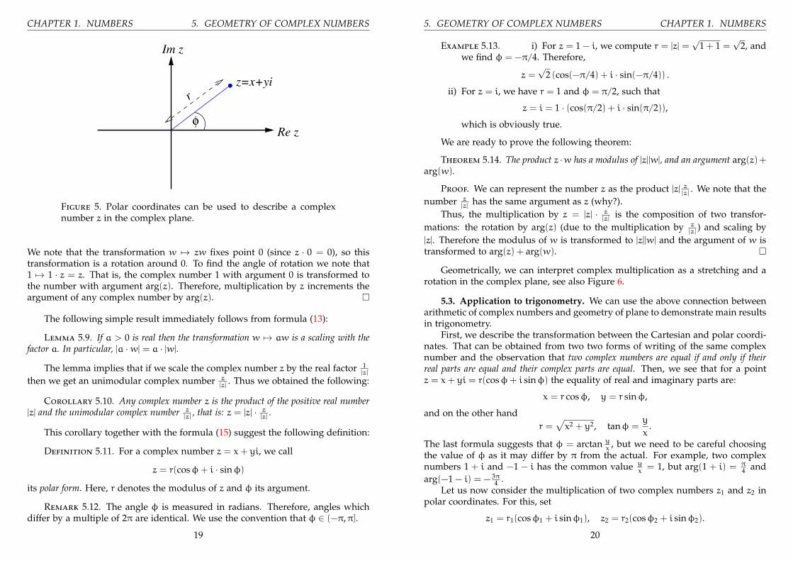
Figure 2. A complex number z can be represented as a point inthe complex plane.
5.1. The complex plane. The graphical presentation is provided by the com-plex plane (or the Argand diagram). Recall that
C = {z = x+ yi, x,y ∈ R},
such that each complex number is characterised by 2 real numbers x and y.Draw rectangular (also known as Cartesian) coordinates on the plane. In the
complex plane the real part x of a number z corresponds to its horizontal compo-nent (along the real axis), whereas the imaginary part y corresponds to its verticalcomponent (along the imaginary axis), see Figure 2.
We can use the complex plane to interpret operations with complex numbersgeometrically.
i) The complex conjugate of a number can be obtained by reflection in thereal axis, see Figure 3.
ii) The addition of 2 complex numbers z1 and z2 has an easy geometric inter-pretation as a translation or using a parallelogram, see Figure 4. There-fore, complex numbers behave like vectors under addition. (We will dis-cuss vectors in the last part of the course.)
Using the properties of the mirror reflection we note:
Lemma 5.1. (1) The conjugation of the complex conjugation returns the com-plex number: z = z.
(2) A complex number is equal to its complex conjugation if and only if it is real:z = z⇔ z ∈ R.
(3) A complex number z satisfy the identity z = −z if and only if it is purelyimaginary.
16

CHAPTER 1. NUMBERS 5. GEOMETRY OF COMPLEX NUMBERS
z=x+yi
Re z
Im z
z=x−yi
Figure 3. A complex number z and its complex conjugate z in thecomplex plane.
Im z
Re z
z
z + z
z1 2
2
1
Figure 4. Addition of two complex numbers z1 and z2.
We will also need the following theorem.
Theorem 5.2. (1) Complex conjugation of the sum of two complex numbers isequal to the sum of their complex conjugates:
z1 + z2 = z1 + z2.
(2) Complex conjugation of the product of two complex numbers is equal to theproduct of their complex conjugates:
z1 · z2 = z1 · z2.
Proof. the first statement follows from the above geometric interpretation ofconjugation and sum. It can be also verified from the formula (11).
The second statement follows from the formula (12). �
17
5. GEOMETRY OF COMPLEX NUMBERS CHAPTER 1. NUMBERS
In order to obtain a clear geometric interpretation for the multiplication anddivision of complex numbers, it turns out, that it is beneficial to introduce newcoordinates in the complex plane; so-called polar coordinates.
5.2. The polar form of a complex number. Instead of using real and imagi-nary part of a complex number z to determine its position in the complex plane,we can also characterise z by its distance r from the origin 0, and the angle φbetween the line connecting z and 0, and the positive real axis, see Figure 5. Thecoordinates (r,φ) are called polar coordinates in the (complex) plane.
First, we note the geometric meaning of modulus, which follows from thePythagoras theorem (do you know its proof?):
Lemma 5.3. The distance from the point z = x + yi to 0 is equal to the modulus|z| =
√zz =
√x2 + y2.
Corollary 5.4. A complex number z and its conjugation z have equal moduli: |z| =|z|.
Combining the previous lemma with the geometric meaning of addition ofcomplex numbers we obtain the next
Corollary 5.5. The distance between two complex numbers z and w is |z−w|.
The known from geometry triangle inequality together with geometric interpre-tation of sum implies the following inequality for moduli of complex numbers:
(14) |z+w| 6 |z|+ |w|.
Thus for the polar coordinates we found that r = |z|, i.e. it is the modulus of z.
Definition 5.6. The angle φ is called the argument of the complex number z,arg(z).
Definition 5.7. A complex z number with the modulus equal 1, that is |z| = 1,is called unimodular. For an unimodular z with an argument arg(z) = φ we have:
(15) z = cosφ+ i · sinφ.
The identity (15) can be considered as a definition of sine and cosine functions.
Theorem 5.8. Multiplication by an unimodular complex number z is a rotation ofthe complex plane by the angle arg(z).
Proof. Take a complex number w. It is transformed by the multiplication tozw. We calculate the modulus:
|zw|2 = zwzw = (zz) · (ww) = |w|2.
So the lengths of a vector is preserved. Furthermore, the distance between pointsis preserved, cf. Cor. 5.5:
|zw1 − zw2| = |z(w1 −w2)| = |z| · |(w1 −w2)| = |w1 −w2|.
18
CHAPTER 1. NUMBERS 5. GEOMETRY OF COMPLEX NUMBERS
z=x+yi
Re z
Im z
r
φ
Figure 5. Polar coordinates can be used to describe a complexnumber z in the complex plane.
We note that the transformation w 7→ zw fixes point 0 (since z · 0 = 0), so thistransformation is a rotation around 0. To find the angle of rotation we note that1 7→ 1 · z = z. That is, the complex number 1 with argument 0 is transformed tothe number with argument arg(z). Therefore, multiplication by z increments theargument of any complex number by arg(z). �
The following simple result immediately follows from formula (13):
Lemma 5.9. If a > 0 is real then the transformation w 7→ aw is a scaling with thefactor a. In particular, |a ·w| = a · |w|.
The lemma implies that if we scale the complex number z by the real factor 1|z|
then we get an unimodular complex number z|z|
. Thus we obtained the following:
Corollary 5.10. Any complex number z is the product of the positive real number|z| and the unimodular complex number z
|z|, that is: z = |z| · z
|z|.
This corollary together with the formula (15) suggest the following definition:
Definition 5.11. For a complex number z = x+ yi, we call
z = r(cosφ+ i · sinφ)
its polar form. Here, r denotes the modulus of z and φ its argument.
Remark 5.12. The angle φ is measured in radians. Therefore, angles whichdiffer by a multiple of 2π are identical. We use the convention that φ ∈ (−π,π].
19
5. GEOMETRY OF COMPLEX NUMBERS CHAPTER 1. NUMBERS
Example 5.13. i) For z = 1 − i, we compute r = |z| =√
1 + 1 =√
2, andwe find φ = −π/4. Therefore,
z =√
2 (cos(−π/4) + i · sin(−π/4)) .
ii) For z = i, we have r = 1 and φ = π/2, such that
z = i = 1 · (cos(π/2) + i · sin(π/2)),
which is obviously true.
We are ready to prove the following theorem:
Theorem 5.14. The product z ·w has a modulus of |z||w|, and an argument arg(z)+arg(w).
Proof. We can represent the number z as the product |z| z|z|
. We note that thenumber z
|z|has the same argument as z (why?).
Thus, the multiplication by z = |z| · z|z|
is the composition of two transfor-mations: the rotation by arg(z) (due to the multiplication by z
|z|) and scaling by
|z|. Therefore the modulus of w is transformed to |z||w| and the argument of w istransformed to arg(z) + arg(w). �
Geometrically, we can interpret complex multiplication as a stretching and arotation in the complex plane, see also Figure 6.
5.3. Application to trigonometry. We can use the above connection betweenarithmetic of complex numbers and geometry of plane to demonstrate main resultsin trigonometry.
First, we describe the transformation between the Cartesian and polar coordi-nates. That can be obtained from two two forms of writing of the same complexnumber and the observation that two complex numbers are equal if and only if theirreal parts are equal and their complex parts are equal. Then, we see that for a pointz = x+ yi = r(cosφ+ i sinφ) the equality of real and imaginary parts are:
x = r cosφ, y = r sinφ,
and on the other handr =
√x2 + y2, tanφ =
y
x.
The last formula suggests that φ = arctan yx
, but we need to be careful choosingthe value of φ as it may differ by π from the actual. For example, two complexnumbers 1 + i and −1 − i has the common value y
x= 1, but arg(1 + i) = π
4 andarg(−1 − i) = − 3π
4 .Let us now consider the multiplication of two complex numbers z1 and z2 in
polar coordinates. For this, set
z1 = r1(cosφ1 + i sinφ1), z2 = r2(cosφ2 + i sinφ2).
20

CHAPTER 1. NUMBERS 5. GEOMETRY OF COMPLEX NUMBERS
Im z
Re z
z2
z
z z21
φφ φφ+
1
1 22
1
Figure 6. Multiplying two complex numbers in the complexplane.
Then using the theorem 5.14 we obtain:
z1 · z2 = r1r2 (cosφ1 cosφ2 − sinφ1 sinφ2 + i(cosφ1 sinφ2 + cosφ2 sinφ1))
= r1r2 (cos(φ1 + φ2) + i sin(φ1 + φ2)) .
This implies the following important trigonometric formulas of addition:
cos(φ1 + φ2) = cosφ1 cosφ2 − sinφ1 sinφ2,
sin(φ1 + φ2) = cosφ1 sinφ2 + cosφ2 sinφ1.
In the special case z1 = z2 = r(cosφ+ i sinφ), we find that
(r(cosφ+ i sinφ))2 = r2 (cos(2φ) + i sin(2φ)) ,
which gives the doubling argument identities:
cos(2φ) = cos2φ− sin2φ, sin(2φ) = 2 cosφ sinφ.
This results can be generalized and yields an important formula for complexnumbers.
Theorem 5.15 (De Moivre’s Theorem). For all complex numbers z = r(cosφ +i sinφ) and all natural numbers n ∈ N, we have
(r(cosφ+ i sinφ))n = rn (cos(nφ) + i sin(nφ)) .
This theorem can be proved using mathematical induction, and we will use itlater to compute complex roots. Next, however, we will take a look at yet anotherrepresentation of complex numbers, which comes from one of the most beautifuland surprising formulas in mathematics.
21
5. GEOMETRY OF COMPLEX NUMBERS CHAPTER 1. NUMBERS
5.4. The exponential form and Euler’s formula. We continue to explore theconnection between geometry and arithmetic of complex numbers. The well-known proposition (Prop. I.5 in Euclid): the base angles of an isosceles triangle areequal (do you know its proof?). It is easy to show the following
Proposition 5.16. If in a triangle ABC, the vertex C belong to the (unique) circlewith the diameter AB, then the angle ACB is right.
Proof. We denote by O the midpoint of AB (see the left drawing on Fig. 7),thenO is the centre of the circle with the diameterAB. By the theorem assumption,the segments OA, OB and OC are equal and we have two pairs of equal angles intwo isosceles triangles (see the illustration). Since the sum of all angles in ABC (asany other triangle) is 180◦, the angle ACB is exactly the half of this, that is it is aright angle. �
OAB
C
OAB
C
OAB
C
Figure 7. The diameter and the right angle.
Also, it is elementary to derive from the isosceles triangle theorem that amongtwo sides of a triangle, the bigger side is opposite to the larger angle (this also followsfrom the sine rule). Using this statement we can show the converse of Prop. 5.16.
Proposition 5.17. If in a triangle ABC the angle C is right then the vertex C belongto the circle with the diameter AB.
You can proof this theorem modifying the proof of Prop. 5.16, see the centraland right drawing on Fig. 7.
The following result easily follows from the geometric meaning of multiplica-tion of complex numbers.
Lemma 5.18. The following conditions are equivalent:(1) Vectors z and w are orthogonal.(2) Re(zw) = 0 (in other words: zw is purely imaginary).
Moreover, if w 6= 0 the above conditions are equivalent to the following:
22

CHAPTER 1. NUMBERS 5. GEOMETRY OF COMPLEX NUMBERS
(3) Re( zw) = 0 (in other words: z
wis purely imaginary).
The imaginary part has a geometric meaning as well:
Lemma 5.19. The following conditions are equivalent:(1) Vectors z and w are co-linear.(2) Im(zw) = 0 (in other words: zw is a real number).
Moreover, if w 6= 0 the above conditions are equivalent to the following:
(3) Im( zw) = 0 (in other words: z
wis a real number).
We already know that zw = z · w. We can show by mathematical inductionthat zn = (z)n for any natural n. Can we extend the meaning of an expression az
for complex z and real a > 0? In view of our previous discussion it is naturally torequest that az = az on top of the usual law of exponents: az+w = az · aw. Fromthese two requirements follows:
Proposition 5.20. Let a > 0 and φ be reals, then the number aiφ shall be unimod-ular.
Proof. Consider the expression z = (aiφ − 1)(a−iφ + 1), we claim that it ispurely imaginary. To this end we will show that z = −z:
z = (aiφ − 1)(a−iφ + 1)
= (a−iφ − 1)(aiφ + 1) (by Thm. 5.2 and az = az)
= (a−iφ − 1)(aiφa−iφ)(aiφ + 1) (since aiφa−iφ = aiφ−iφ = a0 = 1)
= ((a−iφ − 1)aiφ)(a−iφ(aiφ + 1)) (by the associative law)
= (1 − aiφ)(1 + a−iφ) (by the distributive law)
= −(aiφ − 1)(a−iφ + 1)= −z.
If (aiφ− 1)(a−iφ+ 1) is purely imaginary, then by Lem. 5.18 vectors (aiφ− 1) and(aiφ + 1) are orthogonal. But these vectors connect the point aiφ with end-points1 and −1 of the unit circle. By the Prop. 5.17 the orthogonality of vectors impliesthat aiφ belong to the unit circle, i.e. aiφ is an unimodular complex number. �
If aiφ is unimodular, then as we already know aiφ = cosψ+ i sinψ. For someangle ψ, which can be considered as function of φ. The law of exponents and thelaw of complex multiplication tell us that: ainφ = cosnψ+i sinnψ for any naturaln. Thus, ψ shall be a linear function of φ, that means that there is a constant αdetermined solely by a such that ψ = αφ. Clearly, the simplest situation occurs ifα = 1 and then ψ = φ.
23
5. GEOMETRY OF COMPLEX NUMBERS CHAPTER 1. NUMBERS
Definition 5.21. The Euler’s constant e is a real, which satisfies to Euler’s For-mula.
(16) eiφ = cosφ+ i sinφ.
We have arrived at one of the most remarkable formulas in the whole of math-ematics. To hint its importance we mention that the number e also known as thebase of natural logarithms. It is known that e is an irrational number approximatelyequal to 2.718281828. . . . Furthermore, like π, the Euler’s constant is not a root ofany algebraic equation with integer coefficients, such numbers are called transcen-dental. An example of an irrational numbers which is not transcendental is
√2
since it is a root of the equation x2 − 2 = 0 with integer coefficients.Note that Euler’s formula gives us a way to write the polar form of a complex
number in a more compact way.
Definition 5.22. For a complex number z = x+yi = r(cosφ+ i sinφ), we call
z = reiφ
its exponential form.
Remark 5.23.(1) We have discussed 3 equivalent representations of a complex number z,
namely
z = x+ yi, with x,y ∈ R= r(cosφ+ i sinφ), where r = |z|, φ = arg(z)
= reiφ.
(2) De Moivre’s Formula immediately follows from the exponential form.Indeed, the theorem simply follows from the fact that
zn =(reiφ
)n= rn
(eiφ)n
= rneinφ,
and converting this back into polar form.(3) If we set φ = π in Euler’s formula, we get eiπ = cosπ+ i sinπ = −1 or
eiπ + 1 = 0.
This remarkable expression is known as Euler’s identity. It gives a relationbetween the numbers 0, 1, i, e,π and is considered to be one of the mostbeautiful and important mathematical formulas.
5.5. Sketching sets of complex numbers in the complex plane. Before leav-ing this section we consider look at an example of a set of complex numberssketched in the complex plane.
Example 5.24. Sketch the following set in the complex plane
M = { z ∈ C | |z− 1 − i| >√
2 }
24

CHAPTER 1. NUMBERS 6. COMPLEX ROOTS
Figure 8. The set M = { z ∈ C | |z − 1 − i| >√
2 } in the complexplane.
Notice firstly that the complex number z − 1 − i can be written z − (1 + i), i.e. asthe “difference” of two complex numbers. Write z = x + yi with x,y ∈ R. Thusz− 1 − i = (x− 1) + (y− 1)i and so
|z− 1 − i| >√
2 ⇔√
(x− 1)2 + (y− 1)2 >√
2
⇔ (x− 1)2 + (y− 1)2 > 2
(where we have used the fact that (x − 1)2 + (y − 1)2 > 0). Now we note that(x− 1)2 + (y− 1)2 = 2 is the equation of the circle with radius
√2 and centre (1, 1)
in the Cartesian x,y plane. Interpreting this remark in the context of the complexplane thus shows us that the set M is the set of complex numbers lying on thecircle of radius
√2 and centre w = 1 + i. See Figure 8.
6. Complex roots
In the last part of this chapter we discuss how to solve equations for complexnumbers. Of particular interest here are n-th roots of complex numbers.
Definition 6.1. For a number w ∈ C we define its complex n-th roots as thesolutions z of the equation zn = w.
Example 6.2. i) The complex square-roots ofw = 2 are given by {−√
2,√
2}.ii) The complex 4th-roots of w = 1 are {1,−1, i,−i} (you can easily check that
the 4th power of all of these numbers gives w = 1).
So, complex square-roots form a set of complex numbers.
25
6. COMPLEX ROOTS CHAPTER 1. NUMBERS
Remark 6.3. We need to take care with the notation z = n√w for complex
roots. In this notes it is used for the whole set of all roots. Do not confuse thisconcept with the ‘square-root function’ f(x) =
√x, which gives the unique number
y (the only positive real from the set 2√x) and is only defined for non-negative real
numbers x.
6.1. Computation of complex roots. Complex roots of numbers are best com-puted using the exponential form. So, let w = reiφ, let n ∈ N, and let z = ρeiθ bea solution of zn = w. Since, by de Moivre’s Formula
zn = ρneinθ,
we must haveρ = n
√r
(where this root denotes the positive real solution of this equation), and there aren possible solutions for the angle θ
θ ∈{φ+ 2kπn
, with 0 6 k 6 n− 1}
.
In particular, we obtain the important result that every complex number (dif-ferent from zero) has exactly n different n-th roots).
Remark 6.4. Before considering an example let us look informally at why thelast sentence holds (i.e. why every nonzero complex number has exactly n differentn-th roots). Consider w = reiφ, then in fact w = rei·(φ+2kπ) for any integer k (i.e.k ∈ Z). In other words we have infinitely many ways of writing/representing thesame complex number w in exponential (or polar) form. When we are lookingfor the arguments (angles) of the nth roots of w, we are in fact looking for θ suchthat nθ ∈ {φ + 2kπ | k ∈ Z } since we are in effect trying to solve the equationzn = w with z = ρeiθ and w = ei·(φ+2kπ) or, in other words, ρneinθ = ei·(φ+2kπ),(for any k ∈ Z). But looking for θ such that nθ ∈ {φ + 2kπ | k ∈ Z } of coursemeans looking for θ ∈ { φ+2kπ
n| k ∈ Z }. Now if we let k range over the numbers
{0, 1, . . . ,n− 1} only we see that the possible values of θ in this range, i.e. the set
(17){φ
n,φ+ 2πn
. . . ,φ+ 2(n− 1)π
n
}are all distinct. On the other hand if we set k = n and we let θ = φ+2kπ
nthen,
rewriting n for k we see that this is just θ = φ+2nπn
= φn
+ 2π = φn
. But φn
isalready in the set of values picked out for θ by letting k range over the numbers{0, 1, . . . ,n − 1}. In effect, for k > n (or k < 0) the values of θ just repeat somevalue already obtained in the set displayed in (17). So this set is precisely the setof arguments (angles) of the nth roots of w = eiφ.
Example 6.5. Compute all 3√
1 +√
3i. (I.e. solve z3 = w where w = 1 +√
3i.)
26

CHAPTER 1. NUMBERS 6. COMPLEX ROOTS
Solution:i) Transform the number w into polar form: w = 1 +
√3i.
So, |w| = 2, and arg(w) = arctan√
31 = π
3 , and we have w = 2 · eiπ3 .
ii) Compute the roots for 3√
1 +√
3i. In other words solve the equation z3 =
w = 1+√
3i. (Also written as z = 3√
1 +√
3i.) We expect to find 3 differentsolutions z1, z2, z3. Using the formulas above we compute for1 k ∈ {0, 1, 2},
zk+1 = teφk+1
where (the modulus of zk+1)
t =3√
2
and
φk+1 =π3 + 2kπ
3=
π+ 6kπ9
.
(To understand the notation2 here, notice that with k = 0, zk+1 = teφk+1
rewrites as z1 = teφ1 ; with k = 1, zk+1 = teφk+1 rewrites as z2 = teφ2 ; andwith k = 2 zk+1 = teφk+1 rewrites as z3 = teφ3 .)
We thus find that
z1 =3√
2 · eiπ9 ,
z2 =3√
2 · ei(π9 + 23π)
=3√
2 · ei 79π
z3 =3√
2 · ei(π9 + 43π)
=3√
2 · ei 139 π
=3√
2 · e−i 59π,
where for z3 (in the last step) we have subtracted 2π such that the angleφ ∈ (−π,π].
iii) If required, we finally convert the roots z1, . . . , z3 back into Cartesian co-ordinates, that is, into the standard form zk = xk + yki. For example, forz1 = x1 + y1i, we have
x1 =3√
2 cos(π/9) ≈ 1.183938513, y1 =3√
2 sin(π/9) ≈ 0.4309183781,
and so z1 ≈ 1.183938513 + 0.4309183781i.
1The notation k ∈ {0, 1, 2} means “k is in the set {0,1,2}”, in other words “either k = 0 or k = 1or k = 2”.
2You might prefer (as I do) to name the solutions as z0, z1, z2. In this case the notation becomes,
for k ∈ {0, 1, 2}, zk = teφk where φk =π3 +2kπ
3 = π+6kπ9 . I have chosen not to use this notation here
to maintain consistency with the rest of the notes (where solutions are denoted x1, x2 etc).
27
6. COMPLEX ROOTS CHAPTER 1. NUMBERS
Figure 9. The three complex solutions z1, z2 and z3 of z3 = w
(with w = 1 +√
3i).
Remark 6.6. The last example can be represented in the complex plane as inFigure 9. Notice that geometrically the roots z1, z2 and z3 lie on a circle. Alsothat the angle between the roots (in terms of the line connecting each root to theorigin) is precisely 6π
9 , i.e. 2π3 . More generally for n > 1 you will always find 2π
n
separating the (lines to the origin) of the n-many n-th roots of w.
6.2. Solving polynomial equations. Complex roots are of importance for thesolution of polynomial equations. We will only discuss one simple example here.
Example 6.7. Find all complex solutions of z4 − 2z2 + 1 = 3.Solution: For this example, let us first introduce v = z2. Then we obtain an
equation for v
v2 − 2v+ 1 = (v− 1)2 = 3.
We immediately conclude that v−1 is either√
3 or −√
3, such that the two solutionsfor v are
v1 = 1 +√
3, v2 = 1 −√
3.
28

CHAPTER 1. NUMBERS 6. COMPLEX ROOTS
Finally, recalling that v = z2, we arrive at 4 solutions of the equation in z
z1 =√v1 =
√1 +√
3 ,
z2 = −√v1 = −
√1 +√
3 ,
z3 =√v2 =
√1 −√
3 ,
=
√(√
3 − 1) · (−1) ,
=
(√(√
3 − 1))i ,
z4 = −√v2 = −
(√(√
3 − 1))i .
(Note that v2 < 0.)
The computations in this example are pretty straightforward. This is not al-ways the case. Indeed, there is no general method or formula for solving polyno-mial equations of degree greater than 4. (The degree of an equation is the highestpower of z appearing in it.)
On the other hand, it is always true that for an equation of degree n, thereexist n complex solutions. For example, we found 4 solutions for the 4-th orderequation above. This important result is known as the Fundamental Theorem ofAlgebra (Gauss, Argand), which is most naturally proven in the course of ComplexAnalysis.
29
CHAPTER 2
Sequences and Series
Arithmetic of rational numbers, i.e. fractions, is performed according to ex-plicit rules which return precise answers. How this can be extended to irrationalsnumbers. e.g.
√2, π, e? The corresponding is easier to describe in terms of
sequences and their limits.In this part we discuss sequences and series of real numbers. We will mainly
be concerned with the notion of a limit, which is one of the most important con-cepts in mathematics. We will discuss its rigorous definition, analyse properties oflimits and derive conditions for sequences (and series) to have a limit.
1. Sequences of real numbers
1.1. Definition and Examples. A sequence of real numbers is simply an (infi-nite) ordered list of real numbers
(a1,a2,a3, . . .), with an ∈ R for all n ∈ N.
So, in a sequence, we simply have a real number an allocated to each naturalnumber n. More precisely, we can define this as a function
Definition 1.1. A sequence of real numbers is a function a : N → R. For thefunction values we write an := a(n). The whole sequence will be denoted by (an)or (an)n∈N.
In the simplest cases we can define the function can be explicitly written.
Example 1.2. With the rule an = 2n − 1, we obtain the sequence of oddnumbers
a1 = 1, a2 = 3, a3 = 5, a4 = 7, . . . or (1, 3, 5, 7, . . .).Similarly, with an = 1
n, we have
a1 = 1, a2 =12
, a3 =13
, a4 =14
, . . .
If a sequence is given by such a rule of the form an = f(n), then we call thesequence explicitly defined.
An important example of explicitly defined sequence is the sequence of allprime numbers:
a1 = 2, a2 = 3, a3 = 5, a4 = 7, a5 = 9, a6 = 11, . . . .
30
CHAPTER 2. SEQUENCES AND SERIES 1. SEQUENCES OF REAL NUMBERS
Although the sequence is explicitly defined we do not know an analytic mathe-matical expression, which produces an for any n.
Often it is easy to define new elements of sequences from values of previouselements.
Example 1.3. On the other hand, we have already come across the Fibonaccinumbers, that is, the list of numbers
(1, 1, 2, 3, 5, 8, 13, 21, 34, . . .)
This sequence is defined by a recursion as follows:
a1 = 1, a2 = 1, and an = an−1 + an−2 if n > 2.
Hence, in order to compute a100, we need a99 and a98 and all other elements ofthe sequence before that. Such sequences, for which an = g(an−1,an−2, . . . ,an−k)are called recursively or implicitly defined. Sometimes they are also called differenceequation, indicating their more difficult analysis. We also remark, that it is some-times possible to convert recursive definition of a sequence into explicit, whichhas clear advantages. For example, this is possible for Fibonacci numbers (canyou find an explicit formula?).
The next example starts from recursively defined sequence and provide anexplicit formula for it.
Example 1.4. Assume you pay £100 into an account at the beginning of thefirst year. At the end of each year, the bank pays 5% interest. How much moneyis there in the account after n years?
Solution: Let mn denote the money in the account at the end of year n. Letm0 = 100 (in pounds) denote the starting capital. Then
m1 = 1.05 · 100 = 105,m2 = 1.05 · 105 = 110.25,m3 = 1.05 · 110.25 = 115.76, etc.
So, we can define the sequence (mn) recursively by
mn = 1.05 ·mn−1.
On the other hand, a careful look at the elements shows that m2 = (1.05)2 ·m0 andm3 = (1.05)3 ·m0. We conclude that we have in general
mn = (1.05)n ·m0.
This second formula is obviously more convenient, if you want to compute mn forn = 20, 40, 120, . . . . It is easy to generalise this example to an arbitrary geometricprogression an+1 = q ·an, i.e. an+1 = qna1. An arithmetic progression an+1 = an+dcan be treated similarly: an+1 = a1 + nd.
31
1. SEQUENCES OF REAL NUMBERS CHAPTER 2. SEQUENCES AND SERIES
Example 1.5. Assume that a bank agreed to pay 100% interest at the end ofyear on our deposit of £1. Thus, we will get 1+1=£2 at the end of the year. Ifthe bank agreed to add the interest each month proportionally, then our depositwill be multiplied by (1 + 1
12 ) each month, and at the end of year we will get(1 + 1
12 )12 (see the previous example). If the interest will be added every day then,
the final sum will be (1 + 1365 )
365. Motivated by this example, we are interested inthe sequence
(18) an =
(1 +
1n
)n.
Using the binomial formula:
an =(1 + 1
n
)n= 1 + n
1!1n+ (n−1)n
2!1n2 + . . . + (n−k)(n−k+1)...(n−1)n
k!1nk
+ . . . + 1nn
= 1 + 1 + 12!
(1 − 1
n
)+ . . . + 1
k!
(1 − k
n
) (1 − k−1
n
). . .(1 − 1
n
)+ . . . + 1
nn(19)
6 1 + 1 + 12! +
13! + . . . + 1
k! + . . . + 1n! (since
(1 − m
n
)6 1 for m 6 n)
6 1 + 1 + 12 + 1
22 + . . . + 12k−1 + . . . + 1
2n−1 (since k! > 2k−1 for all k)6 1 + 2
= 3.(20)
Thus 2 6 an 6 3 for all n.
Example 1.6. Let a be a positive number and we assume that a > 1, otherwisewe can replace it by 1
a> 1. We want to evaluate
√a from the following procedure.
Put x1 = a, and recursively define:
(21) xn+1 =12
(xn +
a
xn
).
We can show by induction that xn+1 6 xn and the inequality between arithmetic
a b
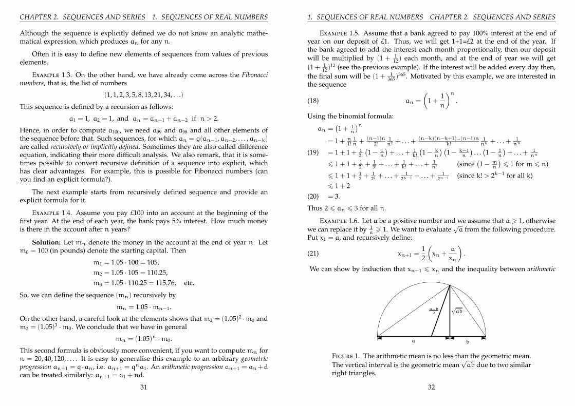
a+b2
√ab
Figure 1. The arithmetic mean is no less than the geometric mean.The vertical interval is the geometric mean
√ab due to two similar
right triangles.
32

CHAPTER 2. SEQUENCES AND SERIES 1. SEQUENCES OF REAL NUMBERS
and geometric means (see Fig. 1) implies that xn+1 >√a (can you do this?), then
|xn+1 −√a| 6 |xn −
√a|. That is, each next number in the sequence will be closer
to√a. Will we get a right approximation from it?
Sometimes, we need some logical operations to define a sequence.
Example 1.7. Here are two examples of sequences of logically defined sequence:
an =
{n2, if n is even;−n2, if n is odd, and bn =
{n, if n is prime;n2, if n is composite.
Note, that that the first sequence also admit an explicit definition: an = (−n)2.Can you find an analytical expression for the sequence (bn)?
There is no any conceptual difficulty to define sequences of complex num-bers as well. However, some of the following results and definitions need to beamended accordingly.
1.2. Properties of sequences. Before we turn to limits of sequences, let usdiscuss two other, more basic, properties of sequences.
Definition 1.8. • A sequence (an) is bounded below, if there exists anumber c ∈ R, such that an > c for all n ∈ N.• A sequence (an) is bounded above, if there exists a number c ∈ R, such
that an 6 c for all n ∈ N.• A sequence (an) is bounded, if there exists a number c ∈ R, such that
|an| 6 c for all n ∈ N.
Remark 1.9. Note that a sequence is bounded, if and only if it is boundedabove and bounded below. The two properties—to be bounded above and below—are logically independent one from another as can be seen from the next example.
Example 1.10. (1) (an) with an = exp(n) is bounded below with c = 0,but not above.
(2) (an) with an = −n is bounded above with c = 0, but not below.(3) (an) with an = (−1)nen is not bounded below or above (it is unbounded).(4) (an) with an = 1/n is bounded.
To see this, note that 1/(n+ 1) < 1/n, 1/1 = 1 and 1/n > 0 for all n ∈ N.Thus |an| 6 1 for all n ∈ N, which shows the boundedness.
(5) The sequence (an) (18) is bounded below by 2 and above by 3 as shownin (20).
(6) The sequence (xn) (21) is bounded above by a and below by√a, as dis-
cussed in that example.
Definition 1.11. • A sequence (an) is called increasing (strictly increas-ing), if
an+1 > an, (an+1 > an) for all n ∈ N.
33
2. LIMITS CHAPTER 2. SEQUENCES AND SERIES
• A sequence (an) is decreasing (strictly decreasing), if
an+1 6 an, (an+1 < an) for all n ∈ N.
• If a sequence is either (strictly) increasing or (strictly) decreasing we callit (strictly) monotone.
As we can see from the next example
Example 1.12. (1) (an) with an = exp(n) is strictly increasing.(2) (an) with an = 1/n is strictly decreasing.(3) The constant sequence with an = 3 for all n is both increasing and de-
creasing.(4) (an) with an = cosn is neither decreasing nor increasing (since cosn
changes sign).(5) The sequence (an) (18) shall be increasing, obviously we will get more
money if the interest is added more frequently. Can you prove this rigor-ously? (Hint: if you compare the formula (19) for n = m and n = m + 1you will see that the later has one more positive term and each other termis bigger than the respective term for n = m. )
(6) The sequence (xn) (21) is strictly decreasing, as discussed in that example.
The property of boundedness is not completely independent from the prop-erty to be monotone.
Exercise 1.13. Show that every monotone sequence is bounded at least eitherabove or below.
We will later discuss how these properties are related to the property of asequence to have a limit. Before, we do so, we first need to introduce this veryimportant property.
2. Limits
2.1. Convergence of sequences. We now define what it means for a sequenceto have a limit. The concept of a limit is the foundation of the whole of calcu-lus. Whenever you compute a derivative, you compute a limit (of the differencequotient); whenever you compute an integral, you compute a limit (of a Riemannsum).
The goal in this part is to discuss this concept in detail, establish properties ofsequences, which have a limit, and find conditions that ensure that a sequence hasa limit.
Definition 2.1. Let (an) ⊂ R be a sequence. We say that an tends (or con-verges) to the limit l ∈ R as n tends to infinity (or that an has the limit l), if forany ε > 0, there exists a number N = N(ε), such that |an − l| < ε for all n > N.
If a sequence has a limit we call it convergent and say that the sequence tendsto l. We write an → l as n→∞ or limn→∞ an = l, if an has the limit l.
34

CHAPTER 2. SEQUENCES AND SERIES 2. LIMITS
Example 2.2. In order to see that this definition agrees with our expectationsabout what it means to have a limit, we will prove that the sequence an = 1/ntends to l = 0 as n → ∞, using the definition. This means, we have to show thatfor all ε > 0, we find a number N, such that |an| < ε for all n > N.
For this, let us choose a fixed but arbitrary ε > 0. Then, for this ε, there existsa number N, such that N > 1
ε(for example, if ε = 0.21, we might choose N = 5).
We claim that with this N, the condition in the definition is satisfied.Indeed, for all n > N, we have 1
n< 1N
, and since N > 1ε
, we also have 1N< ε.
So, we have that an = |an − 0| < 1ε
for all n > N. And since ε was arbitrary,this proves that an → 0 as n→∞.
Discussion of the definition. In short we can write the definition for a sequenceto have limit l as follows:
limn→∞an = l ⇔ ∀ε > 0 ∃N : |an − l| < ε, ∀n > N.
Let us discuss the separate parts of this in detail.• ‘∀ε > 0’: This really means ‘for all small positive numbers ε’. Indeed, if
the inequality |an − l| < ε is satisfied for one ε, then it is automaticallysatisfied for all larger numbers. So, this condition becomes stricter, thesmaller the number ε is.
• ‘∃N . . . ∀n > N:’ This means that the inequality is fulfilled for a whole‘tail’ of the sequence (an).
• ‘|an − l| < ε’: This means l − ε < an < l + ε, like an easy discussion ofthe inequality reveals.
Hence, we can illustrate the property of a sequence to have a limit l as in Figure 2:Give some number ε > 0, we find a number N, such that to the right of the linen = N all elements of the sequence lie in a ’tube’ of diameter 2ε around l. Thedynamic process of convergence (‘a sequence tends to a limit’) has been translatedinto inequalities, which need to be satisfied for tails of sequences.
Definition 2.3. • We say that a sequence diverges, if it has no limitl ∈ R.
• Moreover, a sequence (an) diverges to ∞ (limn→∞ an = ∞), if for allA > 0, there exists a number N, such that an > A for all n > N.
• Similarly, a sequence (an) diverges to −∞ (limn→∞ an = −∞), if for allB < 0, there exists a number N, such that an 6 B for all n > N.
Remark 2.4. Comparing definition 2.1 of the limit and the definition 2.3 asequence divergent to ±∞ we see many similarities. Thus, for those sequenceswe says that they tend to ±∞. The behaviour of divergent sequences (without anylimit) is radically different, see for example an = (−1)n.
Our first result tells us that a convergent sequence has a unique limit.
Lemma 2.5. A sequence (an) has at most one limit.
35
2. LIMITS CHAPTER 2. SEQUENCES AND SERIES
n
N
l
l+ ε
l ε
Figure 2. Convergence of a sequence to the limit l.
Proof. We will prove this indirectly, so—looking for a contradiction—let usassume that there is a sequence (an), such that limn→∞ an = l1 and limn→∞ an =
l2 with l1 6= l2. Then, |l2 − l1| > 0, and we choose ε = 12 |l2 − l1|. Now,
limn→∞an = l1 ⇒ ∃N1 : |an − l1| < ε, ∀n > N1
limn→∞an = l2 ⇒ ∃N2 : |an − l2| < ε, ∀n > N2.
Therefore, for n > max{N1,N2}, we find that |an − l1| < ε and |an − l2| < ε. Butthis means,
|l2 − l1| = |l2 − an + an − l1|
6 |l2 − an|+ |an − l1|
< ε+ ε.
Since |l2 − l1| = 2ε, we have arrived at |l2 − l1| < |l2 − l1|. This is impossible and thedesired contradiction. We conclude that no sequence with two limits can exist. �
Remark 2.6. In the above proof we have used the fact that
|x+ y| 6 |x|+ |y| ∀x,y ∈ R.
This important inequality is known as the triangle inequality.
2.2. Arithmetics of limits. One of the main tasks when faced with a sequenceis to compute its limit (if it exists). In this part we will discuss several simpleresults which help us to achieve this.
36

CHAPTER 2. SEQUENCES AND SERIES 2. LIMITS
Theorem 2.7. Let (an) and (bn) be sequences with an → a and bn → b as n→∞.Then
i) an + bn → a+ b,ii) an · bn → a · b,
iii) anbn→ a
b, if b 6= 0,
as n→∞.
Proof. We will only present the proof for part i) in order to give a flavour ofthe general method.
So, let an → a and bn → b and choose a fixed, but arbitrary ε > 0. Then wefind N1 and N2, such that
|an − a| <ε
2∀n > N1
|bn − b| <ε
2∀n > N2.
Hence, for n > max{N1,N2} we have
a−ε
2< an < a+
ε
2, b−
ε
2< bn < b+
ε
2,
and therefore, after adding the inequalities,
a+ b− ε < an + bn < a+ b+ ε.
In summary, we have found an index N = max{N1,N2}, such that for all n > N,we have |(an+bn)−(a+b)| < ε. Since ε was arbitrary, this proves an+bn → a+bas n→∞. �
Example 2.8. Compute limn→∞ n3−3n2+13n3+4 .
First note that both numerator and denominator of an diverge to infinity, asn→∞. This gives rise to a so-called indeterminate limit, and we need to simplifythe expression, before we can apply the above result. This can be done as follows.
limn→∞ n
3 − 3n2 + 13n3 + 4
= limn→∞ n
3
n3 ·1 − 3 1
n+ 1n3
3 + 4n3
=limn→∞ 1 − limn→∞ 3 1
n+ limn→∞ 1
n3
limn→∞ 3 + limn→∞ 4n3
=13
.
(Note that we have made use of the fact that limn→∞ 1/nk = 0 for k ∈ N. For k = 1we have already discussed the proof. For general k, this will be proved in detailbelow.)
37
2. LIMITS CHAPTER 2. SEQUENCES AND SERIES
n
l
an
bn
cn
Figure 3. Illustration of the sandwich rule.
Another tool for the computation of limits is to compare a difficult sequenceto a simpler one. For example, the following statement is true.
Lemma 2.9. Consider two sequences (an) and (bn) with an > bn for all n ∈ N.Assume that limn→∞ an = a and limn→∞ bn = b. Then a > b.
This lemma remains true in the case that bn diverges to infinity, that is, ifb =∞.
The next result, known as the sandwich rule or squeeze rule, can be used inmany examples to compute limits.
Theorem 2.10 (Sandwich or Squeeze rule). Let (an) and (cn) be sequences withlimn→∞ an = limn→∞ cn = l. Assume further, that for a sequence (bn), we have
an 6 bn 6 cn, ∀n ∈ N.
Then (bn) converges and limn→∞ bn = l.
Proof. Let ε > 0. Then there exists numbers N1 and N2, such that
l− ε < an < l+ ε, ∀n > N1
l− ε < bn < l+ ε, ∀n > N2.
Hence, both inequalities are satisfied for n > max{N1,N2}, and in particular, wehave
l− ε < an 6 bn 6 cn < l+ ε ∀n > max{N1,N2}.This implies limn→∞ bn = l. An illustration of the theorem is given in Figure 3.
�
38

CHAPTER 2. SEQUENCES AND SERIES 2. LIMITS
2.3. Computing limits: Examples. One of the main tasks when given a se-quence, is to compute its limit. In the simplest cases, we can apply Theorem 2.7.In this section, we will have a look at some important, more complicated examples.
i) an = 1nα
with α > 0 as a parameter. Then limn→∞ an = 0.For α = 1 we already checked this, using the definition. If α > 1, then we can
use the sandwich rule to compute the limit, since
1n>
1nα> 0.
Since limn→∞ 1n= limn→∞ 0 = 0, we conclude that limn→∞ 1
nα= 0.
For 0 < α < 1, we also find that limn→∞ 1nα
= 0. This can be proved bychecking the definition of convergence, or by using the general result that for asequence (an) with limn→∞ an = ±∞, we have limn→∞ 1/an = 0. We write thisas ‘1/∞ = 0’. (We will not prove this result.)
ii) an = βn with β ∈ R as a parameter. The sequence diverges for β 6 −1, forother values we have:
limn→∞an =
∞ if β > 11 if β = 10 if |β| < 1
.
There is nothing to prove for β = 1, so we concentrate on the other cases. Letus start with the case β > 1 and set β = 1 + h with some h > 0. Then, using thebinomial theorem,
βn = (1 + h)n = 1 + nh+ . . . + nhn−1 + hn > 1 + nh.
And therefore, limn→∞ βn > limn→∞ 1 + nh =∞.If |β| < 1, then we set β = 1/|β|. Therefore β > 1 and by the above, we have
limn→∞ βn =∞. Now we again apply ‘1/∞ = 0’ to find limn→∞ βn = 0.iii) an = nα
βn, where α > 0 and β > 1. Then limn→∞ an = 0. (This is usually
described as ‘exponential growth beats polynomials growth’.)We will not prove this here, but only note that the proof uses again the bino-
mial theorem (see [1] for more details). Note, however, that the limit is of the form‘∞∞ ’. This is a so-called indeterminate limit. There are no general rules for limitsof this type (see below for more examples), and each case needs to be discussedcarefully.
As an example, let us compute the next limit:
limn→∞ n
10 − 5n2 + 2n
3 · 2n − n= limn→∞ 2n
2n·n10
2n − 5n2
2n + 13 − n
2n=
13
,
applying the above result.iv) an = n
√n = n1/n. Then limn→∞ an = 1.
We note, that the limit is another indeterminate expression, now of the form‘∞0’. For the proof, we again employ the binomial theorem. Firstly note that
39
2. LIMITS CHAPTER 2. SEQUENCES AND SERIES
a1 = 1. Consider an = n√n for n > 1. Note that we can set n
√n = 1+hn, for some
real number hn > 0. Then
n = (1 + hn)n = 1 + nhn +
n(n− 1)2
h2n + . . . + nhn−1
n + hnn.
Thus, n > n(n−1)2 h2
n, which after some transformations leads to hn <√
2n−1 . Since
limn→∞√ 2n−1 = 0, we can apply the sandwich rule to see that limn→∞ hn = 0.
(Formally let (cn) and (bn) be the sequences defined by setting cn = 0 for all
n ∈ N and b1 = 1 and bn =√
2n−1 for n > 1. Then limn→∞ cn = limn→∞ bn = 0
whereas cn 6 an 6 bn for all n ∈ N. So by the Sandwich rule lims→∞an = 0.)This in turn implies that n
√n = 1.
v) an =(1 + 1
n
)n introduced in Example 1.5. We will demonstrate the ex-istence of the limit in Example 2.16, its value e = limn→∞ an is called Euler’sconstant, which is e ≈ 2.718281828 . . . .
This limit is of the form ‘1∞’. In this case, it is not easy to see that the sequenceshould converge at all. It is even more surprising, that the sequence converges toEuler’s number e. We will also derive a different formula for e:
e =
∞∑k=0
1k!
.
vi) an =√n+ 5 −
√n+ 3. Then limn→∞ an = 0. This limit is of the form
‘∞ −∞’. Again, for limits of this type, no general rule exists, and each of themneeds to be discussed separately. Especially, when square-roots are involved, thefollowing method is often successful:
limn→∞
√n+ 5 −
√n+ 3 = lim
n→∞√n+ 5 −
√n+ 3 ·
√n+ 5 +
√n+ 3√
n+ 5 +√n+ 3
=(n+ 5) − (n+ 3)√n+ 5 +
√n+ 3
=2√
n+ 5 +√n+ 3
= 0.
To summarise this section, let us recall the main points to observe, when com-puting limits of sequences.
• If necessary, split the expression for your sequence into as simple conver-gent parts.• If possible, apply Theorem 2.7.• Use the rules ‘1/∞ = 0’ or ‘1/0 =∞’.• If the limit is of one of the following (indeterminate) types
‘∞/∞’, ‘0/0’, ‘0 ·∞’, ‘∞−∞’, ‘1∞’, ‘∞0’,
40

CHAPTER 2. SEQUENCES AND SERIES 2. LIMITS
then no general rules are available. You need to simplify the expressionas much as possible (and maybe use rules like ‘exponential growth beatspolynomial growth’).
Remark 2.11. If I ⊆ R is an interval (i.e. of the real line), f is a continuousfunction over the interval I, and (an) and (bn) are sequences such that
(i) an = f(bn), for all n ∈ N,
(ii) bn ∈ I, for all n ∈ N,
(iii) (bn) converges and limn→∞ bn = b,
then
limn→∞an := lim
n→∞ f(bn)= f
(limn→∞bn
)= f (b)
The point here for this course is that you are not expected to be conversant withthe notion of a continous function. However, in exercises you may come acrossexamples of functions that are continous over an interval of the real line and youcan apply this remark. For example you may come across the following cases:
(1) I = R and f(x) = sin(x), cos(x) or exp(x).
(2) I = [0,+∞) and f(x) =√x.
Remark 2.12. If the sequence (an) has limit a and (cn) is a (infinite) subse-quence of (an) then (cn) also has limit a. For example, if
(i) cn = a2n for all n ∈ N,(ii) cn = an+K for some fixed K ∈ N, e.g. K = 1 or K = 107.
2.4. Convergence criteria. We have introduced the properties of monotonicityand boundedness at the beginning of this part. We will now relate them to theproperty of a sequence to have a limit. The first result is the following.
Lemma 2.13. Every convergent sequence is bounded.
Proof. Assume the sequence (an) has a limit l. Then for all ε > 0 we find anumber N, such that |an − l| < ε for all n > N. Now, let us choose ε = 1. Thenwe find a number N, such that |an − l| < 1 for all n > N. Hence the subsequence(an)n>N is bounded. On the other hand, there are only finitely many elementsa1,a2, . . . ,aN left, and there must exist a maximum or minimum of those finitelymany numbers. Therefore, the sequence (an) is bounded. �
41
2. LIMITS CHAPTER 2. SEQUENCES AND SERIES
So far we have focussed on ways to compute the limit of a sequence. In somecases, however, this computation is very difficult or even impossible to achieve.Then, the next best thing is show that a sequence actually has a limit. (In that case,it makes sense to look for ways to approximate this limit.) We will state one result,which will be of particular importance in the next chapter, when we discuss seriesof real numbers.
Theorem 2.14 (Monotone Convergence). Consider a sequence (an), which is de-creasing and bounded below. Then (an) has a limit.
Similarly, consider a sequence (bn), which is increasing and bounded above. Then(bn) has a limit.
Remark 2.15.(1) In the above theorem, no statement about the location of the limit is made.
This is characteristic for a convergence criterion. It only gives us condi-tions for a sequence to converge.
(2) We can state the theorem in a different way: A monotone sequence eitherdiverges to ±∞ or it has a limit l. (This gives us a connection betweenmonotonicity and convergence.)
(3) We can also ask what happens if a sequence (an) is bounded (but notnecessarily monotone). In this case it can be shown that a subsequenceconverges, but in general not the whole sequence. (This is known as theBolzano–Weierstrass Theorem, but it is beyond the scope of this course.)
We conclude this part with an application of Theorem 2.14.
Example 2.16. We have seen that the sequence an =(1 + 1
n
)n considered inExample 1.5 is monotonically increasing and bounded above by 3. Thus there is alimit, which is called Euler’s constant e.
Example 2.17. Consider the sequence xn defined in Example 1.6. We haveseen that the sequence is monotonically decreasing: xn+1 6 xn. Yet, the sequenceis bounded: xn >
√a. Thus, the sequence has a limit limn→∞ xn = l. Take the
recurrence relation (21) and pass to the limit there:
limn→∞ xn+1 =
12
(limn→∞ xn +
a
limn→∞ xn)
.
Thus the limit l has to satisfy the relation l = 12
(l+ a
l
), that is l2 = a or l = ±√a.
However, since all xn >√a are positive, the limit l have to be positive as well.
Therefore l =√a.
Example 2.18. Let us consider (an), defined by
an+1 =12an(1 − an), a0 =
12
.
It is easy to check the following:
42

CHAPTER 2. SEQUENCES AND SERIES 2. LIMITS
a) If an ∈ [0, 1], then an+1 ∈ [0, 1].b) If an ∈ [0, 1], then an+1 6 an.
Indeed consider (a). Firstly a1 = 12 . Suppose that n > 1 and an ∈ [0, 1]. If an = 0
or 1 then an+1 = 0. Otherwise 0 < an < 1 and so 0 < 1 − an < 1. But this meansthat
0 <12an(1 − an) <
12an .
Thus an+1 ∈ [0, 1]. So by Mathematical Induction we can conclude that an ∈ [0, 1]for all n ∈ N.
Now consider (b). As we have already seen, if an = 0 or 1 then an+1 = 0. Soan+1 6 an (by (a)). Otherwise 0 < 1 − an < 1 (as we have already noted) so that
an+1 =12an(1 − an) <
12an < an .
Thus an+1 6 an for all n > 0.Therefore, the sequence (an) is decreasing, and it is bounded below by c = 0.
Using Theorem 2.14, we conclude that (an) has a limit, say a.In this case, we can also compute the limit a. For this, note first that limn→∞ an =
limn→∞ an+1 (this follows from Rem. 2.12, which is easy to show from the defini-tion of the limit). Hence, we can take the limit in the defining equation to find (forthe second “=” in the equation below)
limn→∞an = lim
n→∞an+1 = limn→∞
(12an(1 − an)
)But then by applying Theorem 2.7 we get that
limn→∞an =
12
limn→∞an(1 − lim
n→∞an)and so since we know that the sequence (an) has a limit, which we denote a (i.e.a = limn→∞ an) we get the equation
a =12a(1 − a).
This equation has the solutions a1 = 0 and a2 = −1, and the only possible limitfor (an) is therefore a = a1 = 0. We have thus shown that (an) converges to 0.
Example 2.19. We shall be careful when using the above technique to eval-uate limits of recursively defined sequences. For example, take the sequence de-fined by an+1 = −an. If we put limn→∞ an+1 = − limn→∞ an we shall concludelimn→∞ an = 0. However, the sequence 1, −1, 1, −1, . . . does not have a limit atall.
43
3. INFINITE SERIES CHAPTER 2. SEQUENCES AND SERIES
3. Infinite Series
Given a sequence, (ak), we have so far investigated the behaviour of (ak) ask → ∞. In some examples, however, we are not interested in the sequence (ak)itself, but in what happens when we add up the elements ak. Adding up, the firstn terms, a1, . . . ,an, we can define
sn = a1 + . . . + an =
n∑k=1
ak.
The number sn is called a partial sum. If we are interested in the sum of all numbersak, then—since adding an infinite quantity of numbers is not possible—we willagain consider a limit process, namely the limit of the sequence of partial sums(sn). This leads to the idea of an infinite series.
3.1. Definition and Examples.
Definition 3.1. Let (ak) be a sequence, and let (as above) sn =∑nk=1 ak
denote the n-th partial sum. The infinite series∑∞k=1 ak is said to converge, if the
sequence of partial sums (sn) converges. We call s = limn→∞ sn the sum of theseries and write
s =
∞∑k=1
ak.
(To denote that∑∞k=1 ak converges, we also use the notation
∑∞k=1 ak <∞.)
If the sequence (sn) diverges to±∞, then we say that the infinite series divergesto ±∞ and write
∑∞k=1 ak = ±∞.
Let us take a look at a few examples.i) Let us take the interval [0, 1] and colour the left half [0, 1
2 ] in blue. Thenwe colour in blue the left half [ 1
2 , 34 ] of the reminder [ 1
2 , 1] and so on. Onthe n-th step the uncoloured part of the interval has the length 1
2n andthe coloured has the length 1
2 + 14 + 1
8 + . . . + 12n . In the limit n → ∞ the
whole interval will be coloured thus we shall agree that:
1 =12+
14+
18+ . . . =
∞∑k=1
12k
.
The same Fig. 4 can be used to illustrate one of Zeno’s paradoxes: Achillesand the Tortoise.
ii) More generally, if ak = qk for some fixed real number q ∈ R, then thecorresponding series
∑∞k=0 q
k is called a geometric series. The geometricseries is one of the rare examples, for which the sum can be computedexplicitly. To see this, recall that
n∑k=0
qk = 1 + q+ q2 + . . . + qn =1 − qn+1
1 − q, if q 6= 1.
44

CHAPTER 2. SEQUENCES AND SERIES 3. INFINITE SERIES
0 112
0 112
34
0 112
34
78
0 112
34
78
1516
Figure 4. Achilles and Tortoise
(If q = 1, then∑nk=0 q
k = n+ 1.)Since we have an explicit formula for the n-th partial sum, we can
now easily investigate its behaviour as n tends to infinity. Since qn → 0for |q| < 1, we obtain the following important result
∞∑k=0
qk =
{1
1−q , if |q| < 1;∞, if q > 1.
(Note that no statement is made for the range q < 1. In this case theseries diverges, but does not approach infinity or minus infinity.)
iii) For ak = 1/k, we find s1 = 1, s2 = 1 + 12 , s3 = 1 + 1
2 + 13 , etc. Obviously,
for the sequence (ak) we have ak → 0, as k → ∞. But what happens tothe sequence of partial sum (sn) as n tends to infinity?
45
3. INFINITE SERIES CHAPTER 2. SEQUENCES AND SERIES
To understand this, we group terms in1∑ak in a clever way:∞∑k=1
1k= 1 (> 1
2 )
+12+
13
(> 14 + 1
4 = 12 )
+14+
15+
16+
17
(> 18 + 1
8 + 18 + 1
8 = 12 )
+18+
19+ . . . +
114
+1
15(> 1
16 + 116 + . . . + 1
16 + 116 = 1
2 )
+1
16+
117
+ . . . +1
30+
131
(> 132 + 1
32 + . . . + 132 + 1
32 = 12 )
+ . . .
So, we can always group terms in the sum, such that they add upto more than 1/2. In particular, if we add up all terms in the sum onthe right-hand side, we have to add up ‘1/2’s infinitely many times. Wetherefore conclude, that the sequence of partial sum is unbounded anddiverges. But this means that the series
∑∞k=1
1k
also diverges.The infinite series ∞∑
k=1
1k
is called the harmonic series, and is an important example of an infiniteseries, for which the corresponding sequence (ak) tends to 0, but theseries
∑ak still diverges.
Remark 3.2. The divergence of the harmonic series is extremely slow.For example, to reach a sum of 4, we have to add up the first 30 terms inthe series. But to reach a sum of 20, we would have to add up 275 millionterms.
Example 3.3. As an application, we want to use the geometric series to provethat
0.99999 . . . = 0.9 = 1
For this, note that the decimal representation 0.9999 . . . describes the number
0.99999 . . . = 0 +9
101 +9
102 +9
103 + . . . = 9 ·∞∑k=1
110k
.
1Note the use of∑ak as shorthand for
∑∞k=1 ak.
46

CHAPTER 2. SEQUENCES AND SERIES 3. INFINITE SERIES
Now, using the formula for the geometric sum and observing that
1100 +
∞∑k=1
110k
= 1 +
∞∑k=1
110k
=
∞∑k=0
110k
,
we indeed find
0.99999 . . . = 9 ·(
11 − 1
10
− 1
)= 9 · 1
9= 1.
As noted above, it is an exception that the sum of an infinite series can becomputed explicitly. Here is some remarkable series with intriguing sums:
e = 1 +12!
+13!
+14!
+15!
+ . . . =∞∑k=1
1k!
;
π
4= 1 −
13+
15−
17+
19− . . . =
∞∑k=1
(−1)k−1
2k− 1;
π2
6= 1 +
122 +
132 +
142 +
152 + . . . =
∞∑k=1
1k2 .
Usually, the main tasks when given an infinite series is to decide whether itconverges or not. We will discuss a variety of criteria for this.
Remark 3.4. It is helpful to remember that the convergence of an infinite series∑∞k=1 ak
is equivalent to the convergence of the sequence of partial sums sn =∑n
k=1 ak. Implication in one way is explicitly required by Definition 3.1. To see the
opposite connection, take an arbitrary sequence (sn) and define a new sequence(an) by the relations:
a1 = sn, and an = sn − sn−1, for n > 1.
We can directly check that (sn) is the sequence of partial sums for the series∑∞k=1 ak. Thus we can use all results for sequences obtained earlier to derive
convergence of series and wise-verse, all new results for series can be used toinvestigate convergence of sequences.
3.2. Properties of (convergent) series. It is not easy to decide whether a seriesconverges. For the example of the harmonic series we have noted above that thedivergence is so slow, that it is almost impossible to detect in numerical experi-ments. We will learn about different tests that can be used for infinite series. Thefirst one is a fairly easy to check condition for divergence.
Lemma 3.5 (Vanishing Test). Consider∑∞k=1 ak. If the infinite series converges,
then limk→∞ ak = 0.
47
3. INFINITE SERIES CHAPTER 2. SEQUENCES AND SERIES
Proof. Let sn =∑nk=1 ak denote the n-th partial sum. By the assumption
in the lemma, the infinite series converges, and therefore limn→∞ sn exists. Butthen—using a standard trick from the theory of convergent sequences—the limitlimn→∞ sn−1 must exist, too, and we have limn→∞ sn = limn→∞ sn−1. Therefore,
0 = limn→∞ sn − lim
n→∞ sn−1
= limn→∞ (sn − sn−1)
= limn→∞
(n∑k=1
ak −
n−1∑k=1
ak
)
= limn→∞
(n−1∑k=1
ak + an −
n−1∑k=1
ak
)= lim
n→∞an.
�
Remark 3.6. Important: You can only use this lemma in the following way
If limk→∞ak 6= 0, then
∑∞k=1 ak cannot converge.
(That is why the result is called the vanishing test.)The fact that limk→∞ ak = 0 does not imply the convergence of the series.
Indeed, for the harmonic series∑∞k=1 ak, the sequence ak = 1/k tends to zero, but
the series diverges to infinity.
In order to discuss further tests, we will first introduce the concept of absoluteconvergence.
Definition 3.7. An infinite series∑∞k=1 ak is called absolutely convergent, if the
series∑∞k=1 |ak| converges.
Obviously, there is only a difference between the two series in the definition,if (ak) contains negative elements (because otherwise |ak| = ak for all k). But inthis case, we can expect the sum
∑∞k=1 ak to be smaller than
∑∞k=1 |ak|, since both
positive and negative numbers are added. In particular, the absolute convergenceof a series implies its convergence. This is exactly what the next lemma states.
Lemma 3.8. If∑∞k=1 |ak| converges, then
∑∞k=1 ak also converges, and we have∣∣∣∣∣
∞∑k=1
ak
∣∣∣∣∣ 6∞∑k=1
|ak|.
In the following we will discuss several criteria for the absolute convergenceof an infinite series. They are useful, because we have just learned that if a seriessatisfies a condition for absolute convergence, then it will also converge.
48

CHAPTER 2. SEQUENCES AND SERIES 3. INFINITE SERIES
Similar to the methods we used for sequences, a main technique is to comparethe terms in an infinite series with terms in a series that is known to converge (orto diverge). Indeed, we have the following theorem.
Theorem 3.9 (Comparison test). Let∑∞k=1 bk be a series of non-negative numbers,
and assume that∑∞k=1 bk converges (i.e.
∑∞k=1 bk < ∞). Furthermore, let
∑∞k=1 ak be
an infinite series, such that |ak| < c · bk, for all k with some c ∈ R. Then the series∑∞k=1 ak is absolutely convergent.
Proof. We consider the partial sums for the series (|ak|). So, let sn =∑nk=1 |ak|
denote the n-th partial sum. Then, since obviously all |ak| > 0, the sequence (sn)is increasing. Moreover,
n∑k=1
|ak| 6n∑k=1
c · bk
= c
n∑k=1
bk
6 c
∞∑k=1
bk.
Hence, the sequence (sn) is bounded, and therefore, by Theorem 2.14, the se-quence (sn) converges. But this implies
∑nk=1 |ak| < ∞, that is, the infinite series
formed using the (ak) is absolutely convergent. �
Before we use this result, let us state an immediate consequence
Lemma 3.10. For the sequence (ck) with ck > 0 for all k ∈ N, assume that∑∞k=1 ck = ∞ (i.e.
∑∞k=1 ck diverges to +∞). Furthermore, assume that for the se-
ries∑∞k=1 ak, we have ak > b · ck for all k ∈ N for some b ∈ R such that b > 0. Then∑∞
k=1 ak diverges, that is,∑∞k=1 ak =∞.
The comparison test leads us to a convergence result for a very important typeof infinite series.
Example 3.11. i) Consider ∞∑k=1
1√k
.
We can use the comparison test with the sequence ck = 1/k. Indeed, wehave
1√k>
1k
, ∀k ∈ N,
and∑∞k=1
1k=∞. Therefore, Lemma 3.10 implies that∞∑
k=1
1√k=∞.
49
3. INFINITE SERIES CHAPTER 2. SEQUENCES AND SERIES
ii) Now, consider ∞∑k=1
1k2 .
To decide about the convergence of this infinite series, we consider thetelescopic series ∞∑
k=1
1k(k+ 1)
.
We have already discussed, that
11 · 2 +
12 · 3 + . . . +
1n(n+ 1)
=n
n+ 1,
and this implies ∞∑k=1
1k(k+ 1)
= limn→∞ n
n+ 1= 1 .
Now, we also have∣∣∣∣ 1(k+ 1)2
∣∣∣∣ =1
(k+ 1)2 61
k(k+ 1),
and so, applying the comparison test (i.e. Theorem 3.9), we get∞∑k=1
1(k+ 1)2 < ∞
However∞∑k=1
1k2 = 1 +
122 +
132 + . . . = 1 +
∞∑k=1
1(k+ 1)2
We thus conclude that ∞∑k=1
1k2 < ∞
(i.e. that the series∑∞k=1
1k2 converges).
The last 2 examples were special cases of a more general result, the proof ofwhich is beyond the scope of this course. Nevertheless, the result is so important,that it cannot be left out.
Lemma 3.12. Consider the infinite series∞∑k=1
1kα
, with α > 0.
Then the series converges, if α > 1, and it diverges for α 6 1.
50

CHAPTER 2. SEQUENCES AND SERIES 3. INFINITE SERIES
Remark 3.13. Note that in the same way as for sequences, the convergence of aseries is—by the very definition—an asymptotic property. So, if any the conditionsabove is only satisfied for a tail of the sequence (ak), that is, for all k greater thansome number K, then we can still use this test to decide about convergence. Inother words, the first 1, 2, . . . ,K terms of the sequence (ak) play no role.
3.3. The ratio test. In the last part of this chapter we will discuss the mostimportant test for the convergence of an infinite series—the ratio test.
Theorem 3.14 (Ratio Test or D’Alembert’s Test). Consider the infinite series∑∞k=1 ak, and assume that the limit
L = limk→∞
|ak+1|
|ak|
exists. Then,• if L < 1, the series
∑∞k=1 ak converges absolutely;
• if L > 1, the series diverges.
Proof. We first consider the case L < 1: The idea of the proof is to comparethe series with an appropriate geometric series. For this, let us choose a numberq, such that L < q < 1. Since |ak+1|
|ak|→ L, and letting ε = q − L, we know (by the
definition of convergence) that there exists a number K ∈ N, such that
L− ε <|ak+1|
|ak|< L+ ε ,
for all k > K. In particular, as L+ ε = L+q−L = q, and setting K = K+ 1, we thusknow that
|ak+1|
|ak|< q ,
for all k > K. In other words|ak+1| < q|ak| ,
for all k > K. Thus we see that |aK+1| < q|aK|, and |aK+2| < q|aK+1| < q2|aK|, and
more generally that, for any number n > 2,
|aK+n| < q|aK+n−1| < q2|aK+n−2| < . . . < qn−1aK+1 < q
n|aK|.
Since q < 1, we can use the comparison test for the series∑∞k=K |ak| with the
convergent geometric series∑∞k=1 q
k. Indeed note that∑∞k=K |ak| can be rewritten
as∑∞k=0 |aK+k| and we see that
|aK+k| 6 |aK| · qk
for all k > 0. Hence by the comparison test Theorem 5 (with the constant c =|aK|) and the fact that
∑∞k=1 q
k converges, we know that the series∑∞k=K |ak| =∑∞
k=0 |aK+k| converges. But this implies that the series∑∞k=1 |ak| converges (see
the above remark). I.e.∑∞k=1 ak converges absolutely.
51
3. INFINITE SERIES CHAPTER 2. SEQUENCES AND SERIES
For the second case, L > 1, we use a similar argument as above to see that there isa number K, such that |ak+1| > |ak| for all k > K. But then ak 6→ 0, and therefore,by the vanishing test, the series does not converge. �
Example 3.15.a) For
∑∞k=1
1k! we have ak = 1
k! , and therefore
|ak+1|
|ak|=
1(k+1)!
1k!
=k!
(k+ 1)!=
1k+ 1
.
Therefore, limk→∞ |ak+1|
|ak|= 0 < 1, and we conclude that the series con-
verges.
b) For∑∞k=1
k4
4k , we have ak = k4
4k , and thus
|ak+1|
|ak|=
(k+ 1)4 · 4kk4 · 4k+1 =
14(k+ 1)4
k4 .
Therefore, limk→∞ |ak+1|
|ak|= 1
4 < 1, and the series converges.
c) For∑∞k=1
(k+1)2
k4+1 we have ak = (k+1)2
k4+1 . In this case
|ak+1|
|ak|=
(k+ 2)2 · (k4 + 1)((k+ 1)4 + 1) · (k+ 1)2
Now, limk→∞ |ak+1|
|ak|= 1. In this case the ratio test does not allow us to
make a statement about whether the series converges or diverges. Herewe need to use a different test. For example, observing that ak = (k+1)2
k4+1 ≈1k2 for large values of k, we could use the comparison test.
3.4. Alternating series. So far, all tests have been for the absolute convergenceof a series. We can use them to decide about the convergence of a series, sinceevery absolutely convergent series must be convergent. A natural question is, ifthere are series that are convergent, but not absolutely convergent.
The answer is yes, and an example can be found in the class of alternatingseries.
Definition 3.16. An infinite series∑∞k=1 ak is called alternating, if ak ·ak+1 <
0.
So, in an alternating series, the terms ak always change sign. Examples aregiven by series of the form∞∑
k=1
(−1)k
k!,
∞∑k=1
(−1)k · k2
k4 + 1, etc.
A convergence test for alternating series goes back to the German mathemati-cian Leibniz.
52
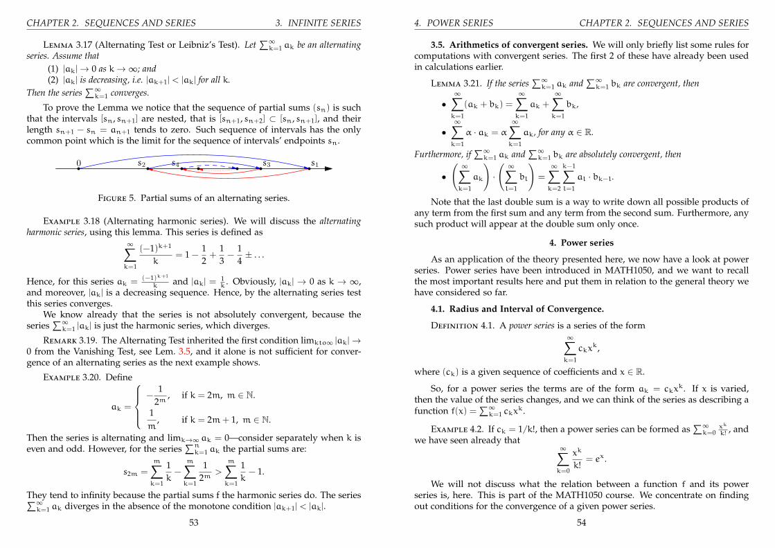
CHAPTER 2. SEQUENCES AND SERIES 3. INFINITE SERIES
Lemma 3.17 (Alternating Test or Leibniz’s Test). Let∑∞k=1 ak be an alternating
series. Assume that(1) |ak|→ 0 as k→∞; and(2) |ak| is decreasing, i.e. |ak+1| < |ak| for all k.
Then the series∑∞k=1 converges.
To prove the Lemma we notice that the sequence of partial sums (sn) is suchthat the intervals [sn, sn+1] are nested, that is [sn+1, sn+2] ⊂ [sn, sn+1], and theirlength sn+1 − sn = an+1 tends to zero. Such sequence of intervals has the onlycommon point which is the limit for the sequence of intervals’ endpoints sn.
s1s2 s3s40
Figure 5. Partial sums of an alternating series.
Example 3.18 (Alternating harmonic series). We will discuss the alternatingharmonic series, using this lemma. This series is defined as∞∑
k=1
(−1)k+1
k= 1 −
12+
13−
14± . . .
Hence, for this series ak = (−1)k+1
kand |ak| =
1k
. Obviously, |ak| → 0 as k → ∞,and moreover, |ak| is a decreasing sequence. Hence, by the alternating series testthis series converges.
We know already that the series is not absolutely convergent, because theseries
∑∞k=1 |ak| is just the harmonic series, which diverges.
Remark 3.19. The Alternating Test inherited the first condition limkto∞ |ak|→0 from the Vanishing Test, see Lem. 3.5, and it alone is not sufficient for conver-gence of an alternating series as the next example shows.
Example 3.20. Define
ak =
−
12m
, if k = 2m, m ∈ N.
1m
, if k = 2m+ 1, m ∈ N.
Then the series is alternating and limk→∞ ak = 0—consider separately when k iseven and odd. However, for the series
∑nk=1 ak the partial sums are:
s2m =
m∑k=1
1k−
m∑k=1
12m
>
m∑k=1
1k− 1.
They tend to infinity because the partial sums f the harmonic series do. The series∑∞k=1 ak diverges in the absence of the monotone condition |ak+1| < |ak|.
53
4. POWER SERIES CHAPTER 2. SEQUENCES AND SERIES
3.5. Arithmetics of convergent series. We will only briefly list some rules forcomputations with convergent series. The first 2 of these have already been usedin calculations earlier.
Lemma 3.21. If the series∑∞k=1 ak and
∑∞k=1 bk are convergent, then
•∞∑k=1
(ak + bk) =
∞∑k=1
ak +
∞∑k=1
bk,
•∞∑k=1
α · ak = α
∞∑k=1
ak, for any α ∈ R.
Furthermore, if∑∞k=1 ak and
∑∞k=1 bk are absolutely convergent, then
•( ∞∑k=1
ak
)·( ∞∑l=1
bl
)=
∞∑k=2
k−1∑l=1
al · bk−l.
Note that the last double sum is a way to write down all possible products ofany term from the first sum and any term from the second sum. Furthermore, anysuch product will appear at the double sum only once.
4. Power series
As an application of the theory presented here, we now have a look at powerseries. Power series have been introduced in MATH1050, and we want to recallthe most important results here and put them in relation to the general theory wehave considered so far.
4.1. Radius and Interval of Convergence.
Definition 4.1. A power series is a series of the form∞∑k=1
ckxk,
where (ck) is a given sequence of coefficients and x ∈ R.
So, for a power series the terms are of the form ak = ckxk. If x is varied,
then the value of the series changes, and we can think of the series as describing afunction f(x) =
∑∞k=1 ckx
k.
Example 4.2. If ck = 1/k!, then a power series can be formed as∑∞k=0
xk
k! , andwe have seen already that ∞∑
k=0
xk
k!= ex.
We will not discuss what the relation between a function f and its powerseries is, here. This is part of the MATH1050 course. We concentrate on findingout conditions for the convergence of a given power series.
54

CHAPTER 2. SEQUENCES AND SERIES 4. POWER SERIES
To decide about the convergence of a power series we can apply the ratio test.With ak = ckx
k (so that |ak| = |ck| · |x|k) we have
|ak+1|
|ak|=
|ck+1|
|ck|· |x|
k+1
|x|k=
|ck+1|
|ck|· |x|.
Thus, assuming limk→∞ |ck+1|
|ck|= l exists, we find that
limk→∞
|ak+1|
|ak|= l|x|.
Therefore,• the series converges for |x| < 1
l,
• the series diverges for |x| > 1l.
Introducing R = 1/l, then the series diverges for x ∈ (−R,R), and it diverges forx < −R or x > R.
Note that R = limk→∞ |ck||ck+1|
. This motivates our next definition.
Definition 4.3. The number
R = limk→∞
|ck|
|ck+1|
is called the radius of convergence of the power series∑∞k=1 ckx
k.
The ratio test does not give any information about what happens for x = ±R.Indeed, these 2 cases have to be studied for each series individually. After such aninvestigation we may establish the interval of convergence. In fact, convergence mayoccur either at both end-points, or only one of them or neither. Thus, in generalthere are four possibilities for the interval of convergence: [−R,R], [−R,R), (−R,R]or (−R,R) depending on the convergence at the end-points.
Example 4.4. As an example we consider the series∞∑k=1
xk
k.
Here, ck = 1/k and we see that
|ck|
|ck+1|=
k
k+ 1→ 1 as k→∞.
I.e. the radius of convergence of the series is R = 1 and we conclude that the seriesconverges if |x| < 1, that is, if x ∈ (−1, 1).(
Note that reasoning directly via the ratio test gives
|ak+1|
|ak|=
k
k+ 1|x|→ 1 · |x| as k→∞.
55
4. POWER SERIES CHAPTER 2. SEQUENCES AND SERIES
Hence the series converges if 1 · |x| < 1, i.e. if |x| < 1.)
In order to find out what happens for x = ±1, we substitute these 2 valuesinto the series:
• x = 1: In this case the series is∑∞k=1
1k
, i.e. it is the harmonic series whichdiverges.• x = −1: Now the series is
∑∞k=1
(−1)k
k.Note that
∞∑k=1
(−1)k+1
k= (−1) ·
∞∑k=1
(−1)k
k.
Thus the series converges as the alternating harmonic series∑∞k=1
(−1)k+1
k
converges (by application of the alternating series test).
In summary, the power series∑∞k=1
xk
kconverges, if x ∈ [−1, 1).
4.2. Illustration: the Euler formula. Let us for the moment return to complexnumbers. The theory of sequences and series can be used for complex numberswith minimal adjustments. Already know that Euler’s number e = 2.71828 . . . canbe defined as the limit of a series
e =
∞∑n=0
1n!
= 1 +11!
+12!
+13!
+14!
+15!
+ . . .
In a similar way we can define the exponential exp(x) of a number x ∈ R as
ex =
∞∑n=0
xn
n!= 1 +
x1
1!+x2
2!+x3
3!+x4
4!+x5
5!. . . .
In particular, we can use this series to evaluate eiπ. Plotting partial sums sn onthe complex plane we can visualise Euler’s identity eiπ + 1 = 0 as on Fig. 6.
Expanding eiφ into the power series we obtain:
exp(iφ) =∞∑n=0
(iφ)n
n!= 1 +
(iφ)1
1!+
(iφ)2
2!+
(iφ)3
3!+
(iφ)4
4!+
(iφ)5
5!. . .
= 1 + iφ1
1!−φ2
2!− iφ3
3!+φ4
4!+ iφ5
5!. . .
= 1 −φ2
2!+φ4
4!∓ . . . + i
(φ1
1!−φ3
3!+φ5
5!∓ . . .
)(22)
where we have used i2 = −1, i3 = −i, etc., and where we have changed the orderof terms in the sum. Comparing (22) with Euler’s formula eiφ = cosφ+ i sinφ weequate the real and imaginary parts of both equations. This gives power series for
56

CHAPTER 2. SEQUENCES AND SERIES 4. POWER SERIES
1
i
s1
s2s3
s4 s5
s6s7
s8 s9
s10
Figure 6. Euler’s identity eiπ + 1 = 0 graphically representedthrough the exponent series.
sine and cosine functions:
sin(x) =
∞∑k=0
(−1)kx2k+1
(2k+ 1)!= x−
x3
3!+x5
5!−x7
7!± . . . ,
cos(x) =
∞∑k=0
(−1)kx2k
(2k)!= 1 −
x2
2!+x4
4!−x6
6!± . . .
57
CHAPTER 3
Vectors
1. Introduction
We often meet a quantity, which has a direction and a magnitude. Standardexamples can be found in mechanics: a force, for example. Think of a force actingon (=pushing) a ball. Then the outcome of this push will depend both on thedirection of the force and on its strength. Another example from physics arevelocities. In geometry, translations of a plane or space are defined by the directionand distance as well.
Such quantities are described by mathematical object called a vectors. Themain properties of vectors that they can be added and multiplied by a number. Inthis context numbers are called scalars.
Graphically, vectors are usually represented by arrows (on the plane or inspace). The direction of the arrow corresponds to the direction of the vector, andits length to the vector’s magnitude.
We will indicate vectors in this script by bold letters, i.e, like a, b, v, etc. Inwriting, there are several options. It is common to denote vectors as ~a, ~b or ~v, or asa, b or v. It does not matter, what method is chosen, but it is important (and veryhelpful) to distinguish vectors from numbers (scalars), in order to avoid confusion,when such quantities are mixed.
We have already met vectors on the plane in Section 5, Chap. 1 and seenthat complex numbers are helpful to describe geometrical properties, cf. Lem. 5.18and 5.19, Chap. 1. To treat vectors in 3D space, which we denote by R3, we will usequaternions. For a geometrical introduction of quaternions see also [?Arnold15a,Part II, p. 52].
In this (elementary) introduction to vectors we will define the main opera-tions with vectors and discuss their relations to the equations for lines, planes andspheres.
2. Quaternions and vectors
To define complex numbers we used the imaginary unit i, such that i2 = −1.To describe vectors in R3 we need three imaginary units i, j and k, which will becalled base quaternions.
58

CHAPTER 3. VECTORS 2. QUATERNIONS AND VECTORS
2.1. Quaternion: introduction. A quaternion is an expression of the form:
(23) u = u0 + u1i+ u2j+ u3k, where u0,u1,u2,u3 ∈ R.
The real number u0 = Re(u) is called the real part ( or scalar part) of the quaternionu. The expression u1i + u2j + u3k = Im(u) is called the imaginary part of thequaternion u. We keep this name to stress the similarity to complex numbers.It may be also called the vector part of the quaternion u. We will show that it isconvenient to identify vectors in R3 with expressions bi + cj + dk, that is withquaternions with vanishing real part.
Similarly to complex case we define the conjugated quaternion:
(24) u = u0 − u1i− u2j− u3k, where u = u0 + u1i+ u2j+ u3k.
We define addition of quaternions component-wise, that is by the formula:
(25) a+ b = (ao + b0) + (a1 + b1)i+ (a2 + b2)j+ (a3 + b3)k,
where
a = a0 + a1i+ a2j+ a3k,b = b0 + b1i+ b2j+ b3k.
We can easily check that such addition is commutative and associative, see (1)and (2). Also we define a multiplication of a quaternion by a real number (scalar)by component-wise multiplication:
(26) ta = ta0+ta1i+ta2j+ta3k, where a = a0+a1i+a2j+a3k and t ∈ R.
We can again verify the commutativity tu = ut, stu = tsu and associativitys(tu) = (st)u of such multiplication.
To make a connection between quaternions and vectors we introduce the con-cept of coordinates and position vectors.
2.2. Position vectors and coordinates. Let us consider the 3-dimensional spaceR3 and denote the coordinate axes as usual by x, y and z. (All of the followingworks in R2 in the same way; we just do not have the z-direction.) Every pointP ∈ R3, can be characterised by its coordinates P = (p1,p2,p3), where p1 denotesthe (signed) distance of P to the y-z plane, p2 is the distance of P to the x-z plane,and p3 is the distance of P to the x-y plane, see Figure 1.
We can associate points in R3 with vectors in R3 by introducing the followingvectors
• i as the vector with magnitude ‖i‖ = 1 in the direction of the x-axis;• j as the vector with magnitude 1 in the direction of the y-axis;• k as the vector with magnitude 1 in the direction of the z-axis.
59
2. QUATERNIONS AND VECTORS CHAPTER 3. VECTORS
z
x
P=(p ,p ,p )
0
y
2 31
p p
p
1 2
3
Figure 1. Coordinates of a point P ∈ R3 and the correspondingposition vector.
Using the vectors (i, j,k), a point in R3 can be associated with its position vector,that is the vector connecting P to the origin O. This vector is denoted by
−→OP, and
if P = (p1,p2,p3), we have
−→OP = p1i+ p2j+ p3k.
We also write−→OP = (p1,p2,p3) as an abbreviation for the position vector. (It does
not really matter, whether to write the position vector as a row vector or as acolumn vector. In this course, we use row vectors.)
Interpreting vectors as position vectors of points in R3, it is now straight-forward to express formulas for the addition of vectors by the triangle rule andaddition of the respective quaternions (25), see the left drawing on Fig. 2. It isworth to notice that addition of vectors can be done either by the triangle rule orthe parallelogram rule—with the same result, see Fig. 3.
Similarly, we can visualise the multiplication by scalar, see the right drawingon Fig. 2. So, by multiplying a vector with a real number, we only change itsmagnitude, but not its direction. More precisely, let ‖a‖ denote the magnitude ofthe vector a. Then
‖ra‖ = |r|‖a‖, for all r ∈ R.
60

CHAPTER 3. VECTORS 3. SCALAR PRODUCT AND VECTOR PRODUCT
a1 b1
a2
b2
a1 + b1
a2 + b2
a1 t · a1
a2
t · a2
Figure 2. Addition and multiplication of vectors through coordinates.
a
ba+b
a)
a
a+b b
b)
Figure 3. Addition of 2 vectors using the parallelogram law in onthe left in a) or, equivalently, the triangle law in panel b).
Example 2.1. For a = i + 3j − k = (1, 3,−1) and b = 2i + 4j − 3k = (2, 4,−3),we have
2a− b = (2, 6,−2) − (2, 4,−3) = (0, 2, 1) = 2j+ k.
Remark 2.2. All of the above applies in a straightforward manner to vectorsin R2 (or more generally to vectors in Rn). In the case of a 2-dimensional vectorwe can simply forget about the k-coordinate and set it to 0 in all formulas.
3. Scalar product and vector product
We have seen in Lem. 5.18 and 5.18, Chap. 1 that product of complex numberscan express the property of vectors to be parallel and orthogonal. We want tointroduce a product of quaternions which will be acting in a similar way.
61
3. SCALAR PRODUCT AND VECTOR PRODUCT CHAPTER 3. VECTORS
3.1. Multiplication of quaternions. If we assume that product is associativeand has the distributive law then it will be enough to define product of basequaternions. Following the complex number case we put
(27) i2 = −1, j2 = −1, k2 = −1.
Furthermore we need to put
(28) ij = k.
The motivation for this can be found in rotations: after we rotate by 180◦ aroundx-axis and by 180◦ around y-axis, the result will be the same as of a single rotationby 180◦ around z-axis. Another way to remember the quaternion multiplication isthrough the formula:
(29) i2 = j2 = k2 = ijk = −1.
We can also use the following mnemonic diagram:
i
jk
The product of two base quaternion is the third one, it is come with the sign + ifwe pass from the first factor to the second along the blue arrows and the sign is −if we go in the opposite direction.
It is an important distinction of quaternion from all other numbers we studiedso far is that quaternion multiplication is not commutative:
(30) ij = −ji, ik = −ki, kj = −jk.
From now on we have enough information for the multiplication of quaternions.First, we multiply both sides of (28) from the left by i and get iij = ik, or −j = ikusing (27). Thus, ki = j by (30). Similarly we get jk = i.
To start, we calculate the product aa of a quaternion and its conjugated (24):
(31) aa = aa = a20 + a
21 + a
22 + a
23, where a = a0 + a1i+ a2j+ a3k.
We obtained the real number. In the special case of vectors:
(a1i+ a2j+ a3k)(−a1i− a2j− a3k) = a21 + a
22 + a
23.
Furthermore, this is a simple application of Pythagoras’ theorem to see that thelast expression gives the square of vector’s length. We will also call this magnitudethe norm of the vector.
Definition 3.1. The norm ‖a‖ of the vector a = (a1,a2,a3) = a1i + a2j + a3kis defined as
(32) ‖a‖ =√−aa =
√aa =
√a2
1 + a22 + a
23.
62
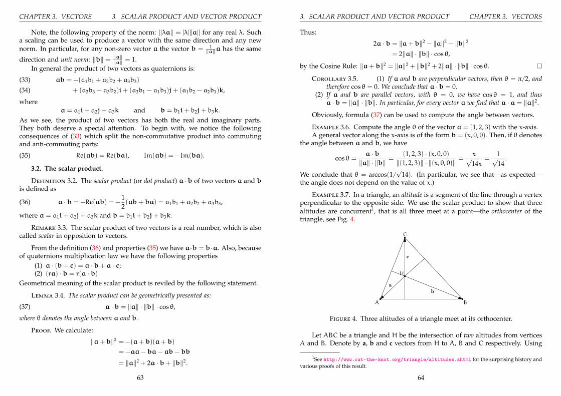
CHAPTER 3. VECTORS 3. SCALAR PRODUCT AND VECTOR PRODUCT
Note, the following property of the norm: ‖λa‖ = |λ|‖a‖ for any real λ. Sucha scaling can be used to produce a vector with the same direction and any newnorm. In particular, for any non-zero vector a the vector b = 1
‖a‖a has the same
direction and unit norm: ‖b‖ = ‖a‖‖a‖ = 1.
In general the product of two vectors as quaternions is:
ab = −(a1b1 + a2b2 + a3b3)(33)
+ (a2b3 − a3b2)i+ (a3b1 − a1b3)j+ (a1b2 − a2b1)k,(34)
wherea = a1i+ a2j+ a3k and b = b1i+ b2j+ b3k.
As we see, the product of two vectors has both the real and imaginary parts.They both deserve a special attention. To begin with, we notice the followingconsequences of (33) which split the non-commutative product into commutingand anti-commuting parts:
(35) Re(ab) = Re(ba), Im(ab) = −Im(ba).
3.2. The scalar product.
Definition 3.2. The scalar product (or dot product) a ·b of two vectors a and bis defined as
(36) a · b = −Re(ab) = −12(ab+ ba) = a1b1 + a2b2 + a3b3,
where a = a1i+ a2j+ a3k and b = b1i+ b2j+ b3k.
Remark 3.3. The scalar product of two vectors is a real number, which is alsocalled scalar in opposition to vectors.
From the definition (36) and properties (35) we have a·b = b·a. Also, becauseof quaternions multiplication law we have the following properties
(1) a · (b+ c) = a · b+ a · c;(2) (ra) · b = r(a · b)
Geometrical meaning of the scalar product is reviled by the following statement.
Lemma 3.4. The scalar product can be geometrically presented as:
(37) a · b = ‖a‖ · ‖b‖ · cos θ,
where θ denotes the angle between a and b.
Proof. We calculate:
‖a+ b‖2 = −(a+ b)(a+ b)
= −aa− ba− ab− bb
= ‖a‖2 + 2a · b+ ‖b‖2.
63
3. SCALAR PRODUCT AND VECTOR PRODUCT CHAPTER 3. VECTORS
Thus:
2a · b = ‖a+ b‖2 − ‖a‖2 − ‖b‖2
= 2‖a‖ · ‖b‖ · cos θ,
by the Cosine Rule: ‖a+ b‖2 = ‖a‖2 + ‖b‖2 + 2‖a‖ · ‖b‖ · cos θ. �
Corollary 3.5. (1) If a and b are perpendicular vectors, then θ = π/2, andtherefore cos θ = 0. We conclude that a · b = 0.
(2) If a and b are parallel vectors, with θ = 0, we have cos θ = 1, and thusa · b = ‖a‖ · ‖b‖. In particular, for every vector a we find that a · a = ‖a‖2.
Obviously, formula (37) can be used to compute the angle between vectors.
Example 3.6. Compute the angle θ of the vector a = (1, 2, 3) with the x-axis.A general vector along the x-axis is of the form b = (x, 0, 0). Then, if θ denotes
the angle between a and b, we have
cos θ =a · b
‖a‖ · ‖b‖ =(1, 2, 3) · (x, 0, 0)
‖(1, 2, 3)‖ · ‖(x, 0, 0)‖ =x√14x
=1√14
.
We conclude that θ = arccos(1/√
14). (In particular, we see that—as expected—the angle does not depend on the value of x.)
Example 3.7. In a triangle, an altitude is a segment of the line through a vertexperpendicular to the opposite side. We use the scalar product to show that threealtitudes are concurrent1, that is all three meet at a point—the orthocenter of thetriangle, see Fig. 4.
A B
C
H
ab
c
Figure 4. Three altitudes of a triangle meet at its orthocenter.
Let ABC be a triangle and H be the intersection of two altitudes from verticesA and B. Denote by a, b and c vectors from H to A, B and C respectively. Using
1See http://www.cut-the-knot.org/triangle/altitudes.shtml for the surprising history andvarious proofs of this result.
64

CHAPTER 3. VECTORS 3. SCALAR PRODUCT AND VECTOR PRODUCT
a
b
b cos θ
θ
Figure 5. Given two vectors a and b with angle θ between them,the projection of b onto a is given by ‖b‖ cos θ.
the scalar product, we write the given orthogonality as
a · (b − c) = 0 and b · (a − c) = 0.
Opening the brackets we obtain:
a · b − a · c = 0 and b · a − b · c = 0.
Subtracting one from another we conclude
b · c − a · c = 0 or, equivalently (b − a) · c = 0.
Thus the line from H to C is the third altitude of the triangle ABC and H is itsorthocenter.
Apart from its connection to the angle between vectors, there is a second geo-metric interpretation of the scalar product. This one is particularly useful forcomputing distances between geometrical objects (like the distance from a pointto a plane or the distance between 2 straight lines). For this, consider the 2 vectorsin Figure 5. Using simple trigonometry, we see that the proportion of b in the di-rection of a (i.e. the length of the perpendicular projection) is given by ‖b‖ cos θ,where θ denotes the angle between a and b. Comparing this with the formula forthe scalar product, we find that
‘projection of b onto a’ =a · b‖a‖ .
65
3. SCALAR PRODUCT AND VECTOR PRODUCT CHAPTER 3. VECTORS
Remark 3.8. So far, all the formulas have been stated for vectors in R3. Asusual, if we deal with 2-dimensional vectors, then we simply ignore the thirdcomponent and find that (v1, v2) · (w1,w2) = v1w1 + v2w2.
3.3. The vector product in R3. Next, we discuss the imaginary part of theproduct (34). In contrast to the scalar product, which is defined for vectors in alldimensions, this vector product is only defined for three-dimensional vectors.
Definition 3.9. Let a,b ∈ R3 be three-dimensional vectors. The vector product(or cross product) a× b is defined by:
a× b = Im(ab) =12(ab− ba)(38)
= (a2b3 − a3b2)i+ (a3b1 − a1b3)j+ (a1b2 − a2b1)k,
In contrast to the scalar product, the vector product of two vectors is anothervector (hence the name).
Lemma 3.10. a × b is a vector, which is perpendicular to both a and b, and whichhas norm
‖a× b‖ = ‖a‖ · ‖b‖ · sin θ,where θ denotes the angle between a and b.
Proof. To establish orthogonality we use the scalar product:
a · (a× b) =12a · (ab− ba)
= −14(a(ab− ba) + (ab− ba)a)
= −14(aab− aba+ aba− baa)
= −14(−‖a‖2b+ b‖a‖2)
= 0.
We used that the multiplication by the real number ‖a‖2 is commutative. Sincethe scalar product vanishes, a and a× b are orthogonal.
We will calculate the vector product in the 2D position. The formula ‖a‖ ·‖b‖ · sin θ gives the area S of parallelogram spanned by vectors a and b. This areacan be also calculated if we will subtract from the area of the rectangle the area ofshaded region on the Fig. 6:
S = (a1 + b1)(a2 + b2) − a1a2 − b1b2 − 2a2b1
= a1a2 + b1a2 + a2 + a1b2 + b1b2 − a1a2 − b1b2 − 2a2b1
= a1b2 − a2b1
�
66

CHAPTER 3. VECTORS 3. SCALAR PRODUCT AND VECTOR PRODUCT
b1
b1a1
a1
b2
b2
a2
a2
S
Figure 6. Area of the parallelogram
Remark 3.11. The direction of a × b is not completely determined by theorthogonality condition, since there are 2 options for the vector to be perpendicularto the two given vectors. In order to remove this ambiguity, the right-hand rule isused to determine the direction of a× b.
Remark 3.12. Another way to express this formula is to make use of deter-minants. If you are familiar with the concept of a determinant, then you can alsoremember that
(a1,a2,a3)× (b1,b2,b3) =
∣∣∣∣∣∣i j ka1 a2 a3b1 b2 b3
∣∣∣∣∣∣ .Example 3.13. Find a vector v, which is perpendicular to the 2 vectors a =
(3, 0, 1) and b = (1, 1,−2) and which has norm ‖v‖ = 1.
We first compute a vector c that is perpendicular to both a and b and adjustthe length in a second step. We use the vector product and set
c = a× b = (3, 0, 1)× (1, 1,−2) = (−1, 7, 3).
(To make sure we have not made a mistake, we can easily check that c ·a = c ·b =0.)
Having computed a vector perpendicular to both a and b, we still need toadjust the norm. So, let v = rc, and let us compute r. We want to have ‖v‖ = 1,and so need to solve
‖v‖ = ‖rc‖ = |r| · ‖c‖ = 1.
67
4. LINES, PLANES AND SPHERES CHAPTER 3. VECTORS
Therefore, we choose r = 1/‖c‖. A simple computation shows ‖c‖ =√
59, and sothe desired vector is
v =1√59
(−1, 7, 3).
Remark 3.14. It worth to highlight the relation between orthogonality and twotypes of products we considered:
(1) To check orthogonality of two vectors a and b we use their scalar product:a · b = 0.
(2) To build a vector orthogonal to vectors a and b we use their vector product:a× b = 0.
4. Lines, Planes and Spheres
In the last part of this chapter, we will discuss the equations for (straight) lines,planes and spheres using vectors.
4.1. Equations for lines. Before deriving equations, let us think about what(geometrical) data we need to characterise a line. There are several options:
i) A point P, and a vector v determine a unique line through P in the direc-tion of v.
ii) Two points P1 and P2 determine the line connecting them.iii) In R2, a line is determined by its slope and a point P, through which it
goes.Let us now see how this data can be turned into equations.
i) For the first case, let Q be an arbitrary point on the line. Then we have
(39)−→OQ =
−→OP + sv,
for some s ∈ R. (As usual,−→OQ denotes the position vector of the point
Q.) If the value of the parameter s is changed, then different points on theline are reached. Because of this, the equation (39) is called the parametricform of a (straight) line.
If, in R3, we have P = (p1,p2,p3) and v = (v1, v2, v3), and if we setQ = (x,y, z) for the unknown point Q, then the parametric from of theline can also be written as
(x,y, z) = (p1,p2,p3) + s · (v1, v2, v3) .
This reads in coordinates
x = p1 + sv1
y = p2 + sv2
z = p3 + sv3,
68
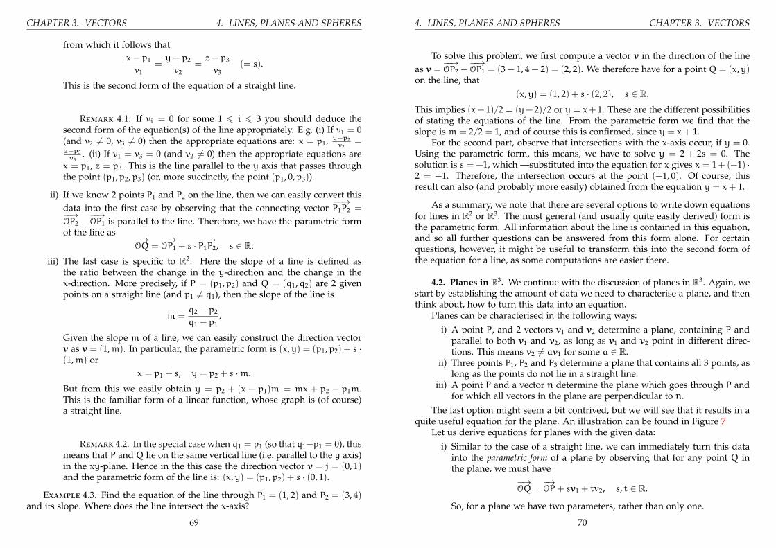
CHAPTER 3. VECTORS 4. LINES, PLANES AND SPHERES
from which it follows thatx− p1
v1=y− p2
v2=z− p3
v3(= s).
This is the second form of the equation of a straight line.
Remark 4.1. If vi = 0 for some 1 6 i 6 3 you should deduce thesecond form of the equation(s) of the line appropriately. E.g. (i) If v1 = 0(and v2 6= 0, v3 6= 0) then the appropriate equations are: x = p1, y−p2
v2=
z−p3v3
. (ii) If v1 = v3 = 0 (and v2 6= 0) then the appropriate equations arex = p1, z = p3. This is the line parallel to the y axis that passes throughthe point (p1,p2,p3) (or, more succinctly, the point (p1, 0,p3)).
ii) If we know 2 points P1 and P2 on the line, then we can easily convert thisdata into the first case by observing that the connecting vector
−−→P1P2 =−−→
OP2 −−−→OP1 is parallel to the line. Therefore, we have the parametric form
of the line as −→OQ =
−−→OP1 + s ·
−−→P1P2, s ∈ R.
iii) The last case is specific to R2. Here the slope of a line is defined asthe ratio between the change in the y-direction and the change in thex-direction. More precisely, if P = (p1,p2) and Q = (q1,q2) are 2 givenpoints on a straight line (and p1 6= q1), then the slope of the line is
m =q2 − p2
q1 − p1.
Given the slope m of a line, we can easily construct the direction vectorv as v = (1,m). In particular, the parametric form is (x,y) = (p1,p2) + s ·(1,m) or
x = p1 + s, y = p2 + s ·m.
But from this we easily obtain y = p2 + (x − p1)m = mx + p2 − p1m.This is the familiar form of a linear function, whose graph is (of course)a straight line.
Remark 4.2. In the special case when q1 = p1 (so that q1−p1 = 0), thismeans that P and Q lie on the same vertical line (i.e. parallel to the y axis)in the xy-plane. Hence in the this case the direction vector v = j = (0, 1)and the parametric form of the line is: (x,y) = (p1,p2) + s · (0, 1).
Example 4.3. Find the equation of the line through P1 = (1, 2) and P2 = (3, 4)and its slope. Where does the line intersect the x-axis?
69
4. LINES, PLANES AND SPHERES CHAPTER 3. VECTORS
To solve this problem, we first compute a vector v in the direction of the lineas v =
−−→OP2 −
−−→OP1 = (3 − 1, 4 − 2) = (2, 2). We therefore have for a point Q = (x,y)
on the line, that(x,y) = (1, 2) + s · (2, 2), s ∈ R.
This implies (x− 1)/2 = (y− 2)/2 or y = x+ 1. These are the different possibilitiesof stating the equations of the line. From the parametric form we find that theslope is m = 2/2 = 1, and of course this is confirmed, since y = x+ 1.
For the second part, observe that intersections with the x-axis occur, if y = 0.Using the parametric form, this means, we have to solve y = 2 + 2s = 0. Thesolution is s = −1, which —substituted into the equation for x gives x = 1+ (−1) ·2 = −1. Therefore, the intersection occurs at the point (−1, 0). Of course, thisresult can also (and probably more easily) obtained from the equation y = x+ 1.
As a summary, we note that there are several options to write down equationsfor lines in R2 or R3. The most general (and usually quite easily derived) form isthe parametric form. All information about the line is contained in this equation,and so all further questions can be answered from this form alone. For certainquestions, however, it might be useful to transform this into the second form ofthe equation for a line, as some computations are easier there.
4.2. Planes in R3. We continue with the discussion of planes in R3. Again, westart by establishing the amount of data we need to characterise a plane, and thenthink about, how to turn this data into an equation.
Planes can be characterised in the following ways:
i) A point P, and 2 vectors v1 and v2 determine a plane, containing P andparallel to both v1 and v2, as long as v1 and v2 point in different direc-tions. This means v2 6= av1 for some a ∈ R.
ii) Three points P1, P2 and P3 determine a plane that contains all 3 points, aslong as the points do not lie in a straight line.
iii) A point P and a vector n determine the plane which goes through P andfor which all vectors in the plane are perpendicular to n.
The last option might seem a bit contrived, but we will see that it results in aquite useful equation for the plane. An illustration can be found in Figure 7
Let us derive equations for planes with the given data:
i) Similar to the case of a straight line, we can immediately turn this datainto the parametric form of a plane by observing that for any point Q inthe plane, we must have
−→OQ =
−→OP + sv1 + tv2, s, t ∈ R.
So, for a plane we have two parameters, rather than only one.
70

CHAPTER 3. VECTORS 4. LINES, PLANES AND SPHERES
=P P P P1 231
P1
P
P3
2
n
y
z
x
Figure 7. A plane can be characterised by 3 points on the planeor by it’s normal vector.
ii) When given 3 points P1, P2, P3, it is easy to write down the parametricform of the plane these points determine. We have
−→OQ =
−−→OP1 + s ·
−−→P1P2 + t ·
−−→P1P3, s, t ∈ R.
iii) If the vector n is perpendicular to the plane, then this means it is perpen-dicular to all vectors in the plane. So, let Q = (x,y, z) be a point on theplane. Then the vector
−→PQ lies in the plane, and we therefore have−→PQ · n = 0.
But since,−→PQ =
−→OQ−
−→OP, this equation can be written as
(−→OQ−
−→OP) · n = 0,
or −→OQ · n =
−→OP · n.
Hence, if we know n = (n1,n2,n3) and P = (p1,p2,p3), then the equationfor the plane reads
n1x+ n2y+ n3z = n1p1 + n2p2 + n3p3.
This is sometimes called the Cartesian form of the equation for a plane.As for the case of lines, we illustrate these general comments using an exam-
ple.
Example 4.4. Find the equation of the plane through A = (1, 0, 0), B = (1, 1, 0)and C = (0, 2,−1), and compute its line of intersection with the plane whose Carte-sian form is 2x+ y = 4.
71
4. LINES, PLANES AND SPHERES CHAPTER 3. VECTORS
We start by deriving the equation of the first plane. Two vectors in this planeare given by
−→AB = (0, 1, 0) and
−→AC = (−1, 2,−1). We use them to compute a
normal vector by letting
n =−→AB×−→AC = (0, 1, 0)× (−1, 2,−1) = (1, 0,−1).
Now, computing n · −→OA = (1, 0,−1) · (1, 0, 0) = 1, we obtain as the equation of theplane
(1, 0,−1) · (x,y, z) = 1, or x− z = 1.In order to find the intersection with the second plane, we note that points in
the intersection need to satisfy both equations describing the planes. This meanswe can find those points by solving the equations
x− z = 1 and 2x+ y = 4
simultaneously. The first equation implies that z = x − 1, whereas the secondequation gives y = 4 − 2x. Therefore, point on the line of intersection are of theform
(x,y, z) = (x, 4 − 2x, x− 1),or, setting x = s as a parameter
(x,y, z) = (0, 4,−1) + s · (1,−2, 1).
This is the parametric form of the line of intersection of the 2 planes.
Notation. If a vector n is perpendicular to a plane S we say that n is a normalvector for the plane S.
Note. Given any plane S whose equation in Cartesian form is
a1x+ a1y+ a3z = b
for some a1,a2,a3,b ∈ R, the vector (a1,a2,a3) is a normal vector for S.
Why? Consider any (fixed) point P = (p1,p2,p3) in the plane. Then
(40) a1p1 + a2p2 + a3p3 = b
Now n is a normal vector for S if and only if−→PQ · n = 0
for any point Q = (x,y, z) in the plane S, if and only if
(−−→OQ−
−→OP) · n = 0
i.e. if and only if(x,y, z) · n = (p1,p2,p3) · n .
i.e. if and only ifn1x+ n2y+ n3z = b
72
CHAPTER 3. VECTORS 4. LINES, PLANES AND SPHERES
by (40). Hence we can take ni = ai for 1 6 i 6 3. In other words
n = (a1,a2,a3) .
Example (i) A normal vector for the plane
3x− 4y+ 5z = 7
is n = (3,−4, 5).
(ii) A normal vector for the plane
2x+ 3z = 0
is m = (2, 0, 3).
4.3. Spheres in R3. Let us start by recalling the equation for a circle in R2. Ifthe circle has centre (x1,y1) and radius r, then points on the circle satisfy
(x− x1)2 + (y− y1)
2 = r2.
Using the 2-dimensional vectors (x,y) and (x1,y1), we can rewrite this as
‖(x,y) − (x1,y1)‖2 = r2.
Hence—as expected—a circle is the set of points that are at distance r from thecentre (x1,y1).
In the same way, a sphere in R3 is the set of points at a certain distance r froma centre (x1,y1, z1). Thus, these points have to satisfy the equation
‖(x,y, z) − (x1,y1, z1)‖2 = r2,
which means(x− x1)
2 + (y− y1)2 + (z− z1)
2 = r2.
Example 4.5. Where does the sphere with centre P = (2,−1, 1) and radiusr = 4 intersect the z-axis?
The equation of the sphere is
(x− 2)2 + (y+ 1)2 + (z− 1)2 = 16.
Points on the z-axis are of the form (0, 0, z), so we need to solve
4 + 1 + (z− 1)2 = 16
This means (z − 1)2 = 11, which has solutions z± = 1 ±√
11. The 2 points ofintersection are therefore
P± = (0, 0, z±) = (0, 0, 1±√
11).
Example 4.6. A sphere with its centre at the origin just touches the plane Swhose Cartesian form is
2x− y− 3z = −1 .What is the radius of the sphere? State its equation.
73
4. LINES, PLANES AND SPHERES CHAPTER 3. VECTORS
Solution. A normal vector for S is
n = (2,−1,−3) .
Hence the line L through O = (0, 0, 0) in the direction of n is given by the equation(in parametric form)
(x,y, z) = (0, 0, 0) + s · (2,−1,−3)
= (2s,−s,−3s) .
Thus L intersects S at the point satisfying
2(2s) − (−s) − 3(−3s) = −1
i.e. where s = − 114 . Hence the intersection is obtained by substituting − 1
14 for s inthe equation of the line L. I.e. the intersection is at the point
(x,y, z) = −1
14(2,−1,−3) .
The distance from the plane to the origin is thus 114
√22 + 12 + 32 = 1√
14. Hence the
equation of the sphere is
x2 + y2 + z2 =1
14.
(i.e. (x− 0)2 + (y− 0)2 + (z− 0)2 = ( 1√14)2) and the radius of the sphere is r = 1√
14.
74

Index
C (complex numbers), 15Im(z) (the imaginary part), 15N (natural numbers), 7Q (rational numbers), 13R (real numbers), 15R3, 59Re(z) (the real part), 15Z (integers), 13cos, 19sin, 19∀ (for all, for every), 37arg (argument), 19∃ (exists), 37i (base quaternion), 59∈ (in, belongs to the set), 7∞ (infinity), 35j (base quaternion), 59k (base quaternion), 59lim (limit), 35n√ (n-th complex root), 27⊂ (subset), 13∑
(sum), 7
absolutelyconvergent series, 49
Achilles and the Tortoise, 45addition
quaternion, 61algebraic
equation, 17algebraically closed, 17alternating
harmonic series, 55series, 53test, 55
altitude of triangle, 65Argand diagram, 17
argument, 19arithmetic
mean, 33operation, 7progression, 33
associativity, 7axiom, 7
baseof natural logarithm, 25quaternion, 59
binary operation, 7Bolzano–Weierstrass
theorem, 43bounded
above sequence, 35below sequence, 35sequence, 35
Cartesiancoordinates, 17equation
plane, 73closed
algebraically, 17commutativity, 7comparison test, 51complexn-th root, 27conjugate, 15number
exponential form, 25polar form, 21
numbers, 15plane, 17
conjugatecomplex, 15
75
CHAPTER 3. INDEX
quaternion, 61constant
Euler’s, see also Euler’s numbercontinuous
function, 43contradiction
proof, by, 13convergence
theorem on monotone convergence, 43convergent
absolutely, infinite series, 49infinite series, 45sequence, 35
coordinatesCartesian, 17polar, 19rectangular, 17
cosine, 19cross product, see also vector product
D’Alembert’s test, see also ration testDe Moivre’s theorem, 23decreasing
sequence, 35diagram
Argand, 17distributive law, 7divergent
infinite series, 45sequence, 37to (minus) infinity
sequence, 37dot product, see also scalar product
equation, 13algebraic, 17plane
Cartesian, 73parametric, 71
solution (root), 13sphere, 75straight line
parametric, 69proportion, 71
Euler’sconstant, see also Euler’s numberformula, 25, 59identity, 25
visualised, 57number, 25, 41, 43, 57
exponential form of complex numbers, 25
Fibonacci numbers, 33formula
Euler’s, 25, 59function
continuous, 43Fundamental Theorem of Algebra, 31
geometricmean, 35progression, 11, 33series, 45
harmonicseries, 47
alternating, 55
imaginarynumber, 15part, 15
imaginary partquaternion, 61
imaginary unit, 15increasing
sequence, 35indirect proof, 13induction
mathematical, 7inequality
triangle, 19, 37infinite
series, 45alternating, 53convergent, 45divergent, 45
infinity, 35integer numbers, 13irrational numbers, 13
lawdistributive, 7of exponents, 25
Leibniz’s test, see also alternating testlimit
arithmetics, of, 37of a sequence, 35
lineequation
parametric, 69proportion, 71
logically defined sequence, 35
magnitude of vector, 59
76

CHAPTER 3. INDEX
mathematical induction, 7mean
arithmetic, 33geometric, 35
modulus, 17monotone
convergence theorem, 43sequence, 35
natural logarithmbase of, 25
natural numbers, 7norm
unit, 65vector, 63
normal vector for a plane, 73number
complex, 15Euler’s, 25, 41, 43, 57imaginary, 15integer, 13irrational, 13natural, 7rational, 13real, 15transcendental, 25
numbersFibonacci, 33
operationarithmetic, 7binary, 7
orthocenter of triangle, 65
paradoxZeno’s, 45
parametricequation
plane, 71straight line, 69
partimaginary, 15
quaternion, 61real, 15
quaternion, 61scalar of quaternion, see also real part of
quaternionvector
quaternion, see also imaginary part ofquaternion
partialsum of an infinite series, 45
planecomplex, 17equation
Cartesian, 73parametric, 71
normal vector, 73polar
coordinates, 19form of complex numbers, 21
position vector, 61power
series, 55radius of convergence, 57
productcross, see also vector productdot, see also scalar productscalar, 65vector, 67
progressionarithmetic, 33geometric, 11, 33
proof, 7by contradiction, 13by induction, 7indirect, 13
quaternion, 61addition, 61base, 59conjugate, 61imaginary part, 61real part, 61scalar part, see also real part of quaternionvector part, see also imaginary part of
quaternion
radius of convergence of power series, 57ratio
test, 53rational numbers, 13real numbers, 15
sequence, of, 31real part, 15
quaternion, 61rectangular
coordinates, 17recursive sequence, 33right-hand rule, 69root
(solution of equation), 13complex, 27
77
CHAPTER 3. INDEX
ruleright-hand, 69squeeze rule, 39squeeze, 39
squeeze rule, 39scalar, 59, 65scalar part quaternion, see also real part of
quaternionscalar product, 65sequence, 31
bounded, 35above, 35below, 35
convergent, 35decreasing, 35
strictly, 35divergent, 37
to (minus) infinity, 37explicitly defined, 31implicitly defined, see also recursive
sequenceincreasing, 35
strictly, 35limit, of, 35logically defined, 35monotone, 35
strictly, 35of real numbers, 31recursively defined, 33tends to, 35
(minus) infinity, 37series
alternating, 53harmonic, 55
convergent, 45absolutely, 49
divergent, 45geometric, 45harmonic, 47
alternating, 55infinite, 45power, 55
radius of convergence, 57tail, 53telescopic, 51
set, 7sine, 19sphere, 75
equation, 75squeeze rule, 39
strictlydecreasing
sequence, 35increasing
sequence, 35monotone
sequence, 35sum
partial, of an infinite series, 45
tailof series, 53
telescopicseries, 51
testalternating, 55comparison, 51D’Alembert’s, see also ration testLeibniz’s, see also alternating testratio, 53vanishing, 49, 55
theoremBolzano–Weierstrass, 43De Moivre’s, 23Fundamental of Algebra, 31monotone convergence, 43
transcendental number, 25triangle
altitude, 65inequality, 19, 37orthocenter, 65
unimodular, 19unit
imaginary, 15norm, 65
vanishing test, 49, 55vector, 59
cross product, see also vector productmagnitude, 59norm, 63normal for a plane, 73position, 61product, 67
dot, see also scalar productscalar, 65
vector partquaternion, see also imaginary part of
quaternion
Zeno
78

CHAPTER 3. INDEX
paradoxes, 45
79
Bibliography
[1] F.M. Hart, Guide to analysis, Macmillan Mathematical Guides Series, Palgrave, 2001. ↑43[2] Georg Polya, How to solve it, Doubleday Anchor Books, New York, 1957. ↑
80