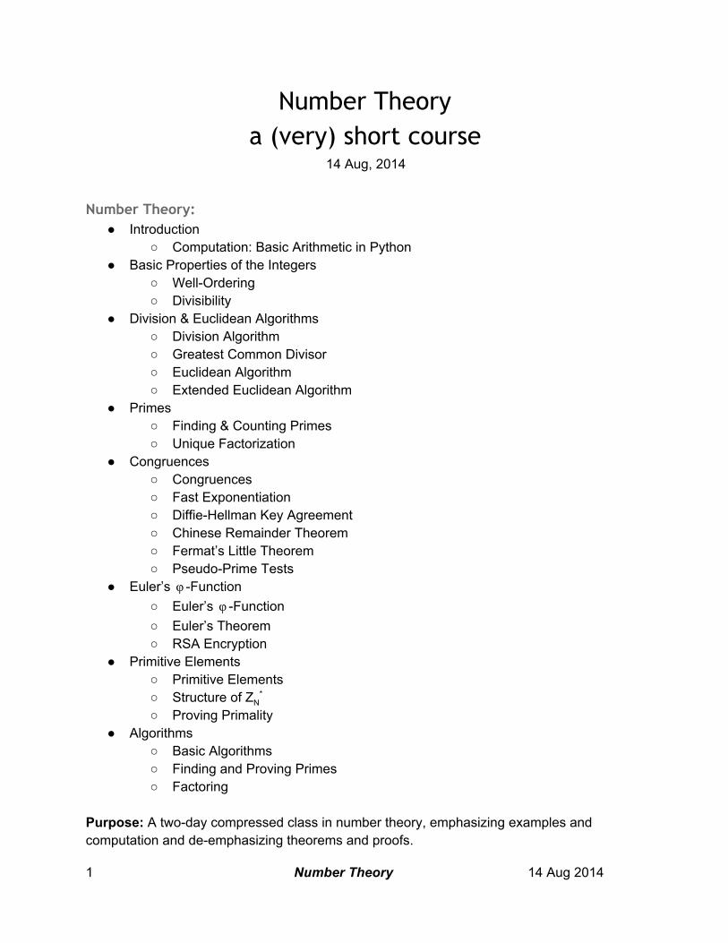
Number Theory a (very) short course

14 Aug, 2014

Number Theory: Introduction

Computation: Basic Arithmetic in Python Basic Properties of the Integers

Well­Ordering Divisibility

Division & Euclidean Algorithms Division Algorithm Greatest Common Divisor Euclidean Algorithm Extended Euclidean Algorithm

Primes Finding & Counting Primes Unique Factorization

Congruences Congruences Fast Exponentiation Diffie­Hellman Key Agreement Chinese Remainder Theorem Fermat’s Little Theorem Pseudo­Prime Tests

Euler’s ­Functionφ Euler’s ­Functionφ Euler’s Theorem RSA Encryption

Primitive Elements Primitive Elements Structure of ZN

* Proving Primality

Algorithms Basic Algorithms Finding and Proving Primes Factoring

Purpose: A two­day compressed class in number theory, emphasizing examples and computation and de­emphasizing theorems and proofs.

1 Number Theory 14 Aug 2014

Number Theory Elementary Number Theory is the study of the integers and the properties they have under addition, multiplication and division. While the larger field of number theory has many more subjects, this small cast of characters yields a very rich structure. While the goal of this course is limited to elementary number theory, we may from time to time bring in examples from the broader theory, if only to emphasize or illustrate some property of the integers by contrasting it with these other examples. There are a number of approaches to number theory. We choose an approach which de­emphasizes the theory, deferring most proofs to another day. Computations and applications are emphasized, as this is what has caused the great interest in number theory in the past few decades.

Computations with Python

In order to deal easily with examples large enough to have interesting properties, it helps to have an aid in computation. While many tools will work, a particularly appropriate one is Python ­ it is available on most machines (generally pre­installed on UNIX/Linux), allows interactive use and has arbitrary sized integers.

>>> (8+7) % 13 # The remainder of dividing (8+7) by 13 >>> 1234567//123 # Divide 1234567 by 123 without remainder >>> a=125; b=35; q=a//b; a=a­q*b; [a,b] # Euclidean Algorithm [20, 35] >>> q=b//a; b=b­q*a; [a,b] [20, 15] >>> a=a%b; [a,b] # The same, just written differently [5, 15] >>> 2**123 # 2 to the 123rd power 10633823966279326983230456482242756608L

The capabilities of Python can also be extended with libraries which are available for this class. >>> import numbthy >>> numbthy.factors(2**113­1) # factor a Mersenne number [3391L, 23279L, 65993L, 1868569L, 1066818132868207L]

A very sophisticated extension of Python which is particularly suitable for computations in number theory and algebra is the SAGE system. This is freely available both on the outside [http://www.sagemath.org] and on the inside.

sage: factor(2**113­1) 3391 * 23279 * 65993 * 1868569 * 1066818132868207

2 Number Theory 14 Aug 2014

sage: euler_phi(2**113­1) 10380922495821490560709669174725120

Basic Properties of the Integers

We will be satisfied with an intuitive description of the integers. More thorough developments of the basic properties of the integers can be found in the first chapter or appendices of most number theory books.

Well-Ordering

The natural numbers are the non­negative integers starting with zero, 0,1,2,3,.... (Some people define the natural numbers as excluding zero.) The natural numbers are blessed with addition, multiplication and an order which plays well with both of these operations.

Def: Given integers a and b, we say that a is less than or equal to b, denoted a b, if≤ there is some natural number c such that b=a+c. If c is a non­zero natural number we say that a is less than b, denoted a<b.

Well­Ordering of the Natural Numbers: Any subset of the natural numbers will have a least element.

The integers are the natural (pun unintended) extension of the natural numbers, supplementing them with the negative integers. Thus the integers, denoted Z (for the German word Zahlen, or number) are the set ..., ­3, ­2, ­1, 0, 1, 2, 3, …, together with the usual addition, subtraction, multiplication, (sometimes) division and the usual order. So we get a similar well­ordering property for the integers ­ any set of integers with a lower bound contains a least element.

Well­Ordering of the Integers: Any subset of the integers with a lower bound will have a least element.

Divisibility

While we can always add, subtract and multiply two integers, we cannot always divide them. The question of when one integer divides another is deeper than it seems.

Def: a divides b (denoted “a|b”) if there exists some integer x such that b=ax. If a divides b we say that a is a divisor of b.

Thus 5 divides 15 and 20 divides 100, but 3 doesn’t divide 100.

3 Number Theory 14 Aug 2014

Just using the definition of divisibility you should be able to prove (most of) the elements of the following theorem.

Thm: (Properties of Divisibility) 1) a|b a|bc⇒ 2) a|b and b|c a|c [Read: If a divides b and also b divides c, then a divides c.]⇒ 3) a|b and a|c x,y, a|(bx+cy) [Read: If a divides b and also a divides c then for⇒ ∀

any integers x and y we have a divides (bx+cy)] 4) a|b and b|a => a= b± 5) a|b, a>0, b>0 a b [Read: If a divides b and also a is positive and also b is⇒ ≤

positive, then a is either b or negative b.] 6) m 0 (a|b ⇔ ma|mb) [Read: If m is non­zero, then a divides b if and only if ma=/ ⇒

divides mb.] proof:

1) If a|b then there exists some integer x such that b=ax So bc = axc So bc = a(cx), so there is some integer z=cx such that (bc)=az Thus a|bc ♠

[Note that only properties (iv) and (v) use anything beyond the definition of divisibility. We can define divisibility for more general rings, such as the polynomials, and get the same properties.]

Problem: Prove the various properties of divisibility.

Division & Euclidean Algorithms

In addition to divisibility properties, the integers have something we tend to take for granted ­ a division algorithm.

Thm: (Division Algorithm) Given integers a, b with a>0, there are unique integers q and r such that b=qa+r and 0 r<a. If a does not divide b then r 0.≤ =/ proof: Consider the set of integers b­na | n an integer. This set looks like a ladder with fixed step size a, starting at b. (This set is a simple example of a lattice.) Clearly there will be a smallest positive or zero element and largest negative or zero element. If either (actually both) is zero, then b=qa, where q is the (signed) number of steps from b to 0. If neither is zero, then let q be the (signed) number of steps from b to the smallest positive element and let r be the (positive) remainder. As the step size is a and we have chosen the smallest positive element, it must be less than a away from 0, so r<0.♠ (This is a plausible proof, but note that it requires a well­ordering property of sets of positive integers.)

4 Number Theory 14 Aug 2014

As a simple example of this line of reasoning, consider how we might divide b=14 by a=4. We would construct the (infinite) set 14+4n = ..., 14­(­2)4=22, 14­(­1)4=18, 14, 14­(1)4=10, 14­(2)4=6, 14­(3)4=2, 14­(4)4=­2, 14­(5)4=­6, .... The smallest positive element is 14­(3)4=2. Thus q=3 and r=2. A few other examples:

if a=3 and b=35 we have q=11 and r=2, as 35=(11)(3)+2 if a=11 and b=­325, then q=­29 and r=7, as ­325=(­29)(11)+7

This of course is not the way we actually perform division. It’s worth thinking through how to write an algorithm which, given only addition, subtraction and multiplication, will implement division.

Problem: Outline an algorithm which implements integer division, returning both quotient and remainder, using only addition, subtraction and multiplication.

The division algorithm is actually a wonderful tool ­ through its use in the Euclidean algorithm it is the basis of much of computational number theory. In order to see how unique it is, consider how you would write a division algorithm for the set of single­variable polynomials with integer coefficients, Z[x]. (Hint: There isn’t a division algorithm in Z[x] ­ try to divide 3x2+2x+1 by 2x+1.)

Greatest Common Divisor

Defn: The greatest common divisor, GCD, of two positive integers a and b is an integer d such that:

1. d | a and d | b 2. If c | a and c | b then c≤d

We can easily show that the GCD exists, using the following reasoning. The set of common divisors of two numbers a and b is non­empty (1 is a common divisor). The set of common divisors is bounded above by the least of |a| and |b|. Thus we can apply the well­ordering principle to the set of common divisors (strictly speaking, rather than finding the maximal element of this set we might have to find the minimal element of the set of their negatives, but that is a minor detail). (The GCD is sometimes also called the Greatest Common Factor, GCF.)

Thm: (Bezout's Thm [a restricted form]) There exist x and y such that gcd(a, b) = ax+by. proof: Consider the set ax+by | x, y ∈ Z Choose x0, y0 so that ax0+by0 is the least positive element (well ordering again) Call this element k = ax0+by0 We now prove that k|a and k|b

5 Number Theory 14 Aug 2014

Assume the converse ­ that k does not divide a So ∃ q, r with 0<r<k and r = a­kq = a­q(ax0+by0) = a(1­qx0) + b(­y0) So r is a positive element of the set which is smaller than k (contradition) Thus k|a and similarly k|b So k | gcd(a,b)♠

This of course gives us a proof that the gcd of two numbers is some linear combination of the numbers, but has no computational value as it doesn’t tell us how to find this linear combination. In a great number of rings we are left sitting here, knowing of the existence of the gcd but unable to practically compute it. The beauty of the integers (and a limited set of other useful rings) is that we have an efficient way of computing these values ­ the Euclidean Algorithm.

Euclidean Algorithm

The Euclidean algorithm is simple and has been around a long time, but it is central to effectively performing computations over the integers, in particular any factoring algorithm. This is somewhat amusing, as the conventional way that students are taught to compute a GCD starts with factoring the numbers. The Euclidean algorithm for computing the GCD of two numbers a and b is a recursive operation. We observe that gcd(a­b,b) = gcd(a,b). If a was larger than b then a­b is less than a, and computing gcd(a­b,b) is a smaller problem than computing gcd(a,b). We keep subtracting b from a until the result is smaller than b. Or we could just jump ahead over all the steps, use the division algorithm to divide a by b, replacing a by the remainder r, and note that gcd(a,b) = gcd(r,b). But now r is less than b, so we can reverse their roles and continue the process. At each step the values being computed with are shrinking ­ eventually one of the two of them is zero. At this point the other value is the desired GCD value because:

Lemma: gcd(a,0) = a Lemma: gcd(a,b­a)=gcd(a,b) proof: g = gcd(a,b) ⇒ (g | a) and (g | b) ⇒ a = ng and b = mg for some n and m So if a = qb + r then r = a ­ qb, so r = ng ­ qmg = g(n­qm) So (g | r) ⇒ (g | gcd(r,b)), i.e. (gcd(a,b) | gcd(r,b)) Similarly, we can show that (gcd(r,b) | gcd(a,b)) Thus gcd(a,b) = ± gcd(r,b)) As both are positive, we have gcd(a,b) = gcd(r,b) ♠

An example of this process which computes gcd(135,24):

6 Number Theory 14 Aug 2014

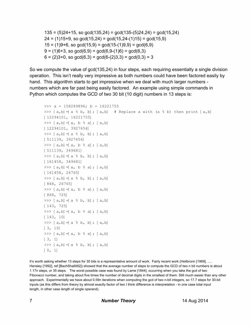
135 = (5)24+15, so gcd(135,24) = gcd(135­(5)24,24) = gcd(15,24) 24 = (1)15+9, so gcd(15,24) = gcd(15,24­(1)15) = gcd(15,9) 15 = (1)9+6, so gcd(15,9) = gcd(15­(1)9,9) = gcd(6,9) 9 = (1)6+3, so gcd(6,9) = gcd(6,9­(1)6) = gcd(6,3) 6 = (2)3+0, so gcd(6,3) = gcd(6­(2)3,3) = gcd(0,3) = 3

So we compute the value of gcd(135,24) in four steps, each requiring essentially a single division operation. This isn’t really very impressive as both numbers could have been factored easily by hand. This algorithm starts to get impressive when we deal with much larger numbers ­ numbers which are far past being easily factored. An example using simple commands in Python which computes the GCD of two 30 bit (10 digit) numbers in 13 steps is:

>>> a = 158289896; b = 16221755 >>> [a,b]=[a % b, b]; [a,b] # Replace a with (a % b) then print [a,b] [12294101, 16221755] >>> [a,b]=[a, b % a]; [a,b] [12294101, 3927654] >>> [a,b]=[a % b, b]; [a,b] [511139, 3927654] >>> [a,b]=[a, b % a]; [a,b] [511139, 349681] >>> [a,b]=[a % b, b]; [a,b] [161458, 349681] >>> [a,b]=[a, b % a]; [a,b] [161458, 26765] >>> [a,b]=[a % b, b]; [a,b] [868, 26765] >>> [a,b]=[a, b % a]; [a,b] [868, 725] >>> [a,b]=[a % b, b]; [a,b] [143, 725] >>> [a,b]=[a, b % a]; [a,b] [143, 10] >>> [a,b]=[a % b, b]; [a,b] [3, 10] >>> [a,b]=[a, b % a]; [a,b] [3, 1] >>> [a,b]=[a % b, b]; [a,b] [0, 1]

It’s worth asking whether 13 steps for 30 bits is a representative amount of work. Fairly recent work (Heilbronn [1969], …, Hensley [1992], ref [BachShallit92]) showed that the average number of steps to compute the GCD of two n bit numbers is about 1.17n steps, or 35 steps. The worst possible case was found by Lame [1844], occurring when you take the gcd of two Fibonacci number, and taking about five times the number of decimal digits in the smallest of them. Still much easier than any other approach. Experimentally we have about 0.59n iterations when computing the gcd of two n­bit integers, so 17.7 steps for 30­bit inputs (as this differs from theory by almost exactly factor of two I think difference is interpretation ­ in one case total input length, in other case length of single operand).

7 Number Theory 14 Aug 2014

Writing out this algorithm carefully we get:

Algorithm: (Computing GCD(a,b)) [Euclidean Algorithm] If a < b then swap a and b Repeat while b > 0 q ← ⌊a/b⌋ (integer quotient of a and b)

a ← a ­ qb swap a and b

(b is now equal to zero and a to the gcd) print "gcd is", a

And writing it in Python as a recursive function (one which calls itself): >>> def gcd(a,b): ... if a == 0: ... return b ... return gcd(b % a, a) >>> gcd(1234567892123450,987654322198765) 5

Extended Euclidean Algorithm

Recall Bezout’s Theorem, which tells us that the GCD of two numbers can be expressed as a linear combination of them. Unfortunately, the statement and proof of Bezout’s theorem don’t give us an effective way to compute the coefficients of this linear combination, just that it exists.

Thm: (Bezout's Thm [a restricted form]) There exist x and y such that gcd(A, B) = Ax+By.

Happily, a careful application of the Euclidean Algorithm while keeping side notes is just what we need to compute this linear combination. This is called the Extended Euclidean Algorithm, sometimes denoted XGCD. We start with the following observation:

Lemma: If a=xaA+yaB and b=xbA+ybB, then (a­qb)=(xa­qxb)A+(ya­qyb)B Recall that a step of the Euclidean Algorithm replaces a with (a­qb) for steps when a is larger than b and where q is the integer quotient of a by b. If we start the process with a=A, xa=1, ya=0, b=B, xb=0 and yb=1, then we have the initial relation a=xaA+yaB and b=xbA+ybB. At each step we replace (viewing a as the larger of a and b, and q as their integer quotient) a<­a­qb, xa<­(xa­qxb) and ya<­(ya­qyb). The values of a and b act as in the original Euclidean Algorithm, so eventually one of them will become zero, at which point the other will have the value GCD(A,B).

8 Number Theory 14 Aug 2014

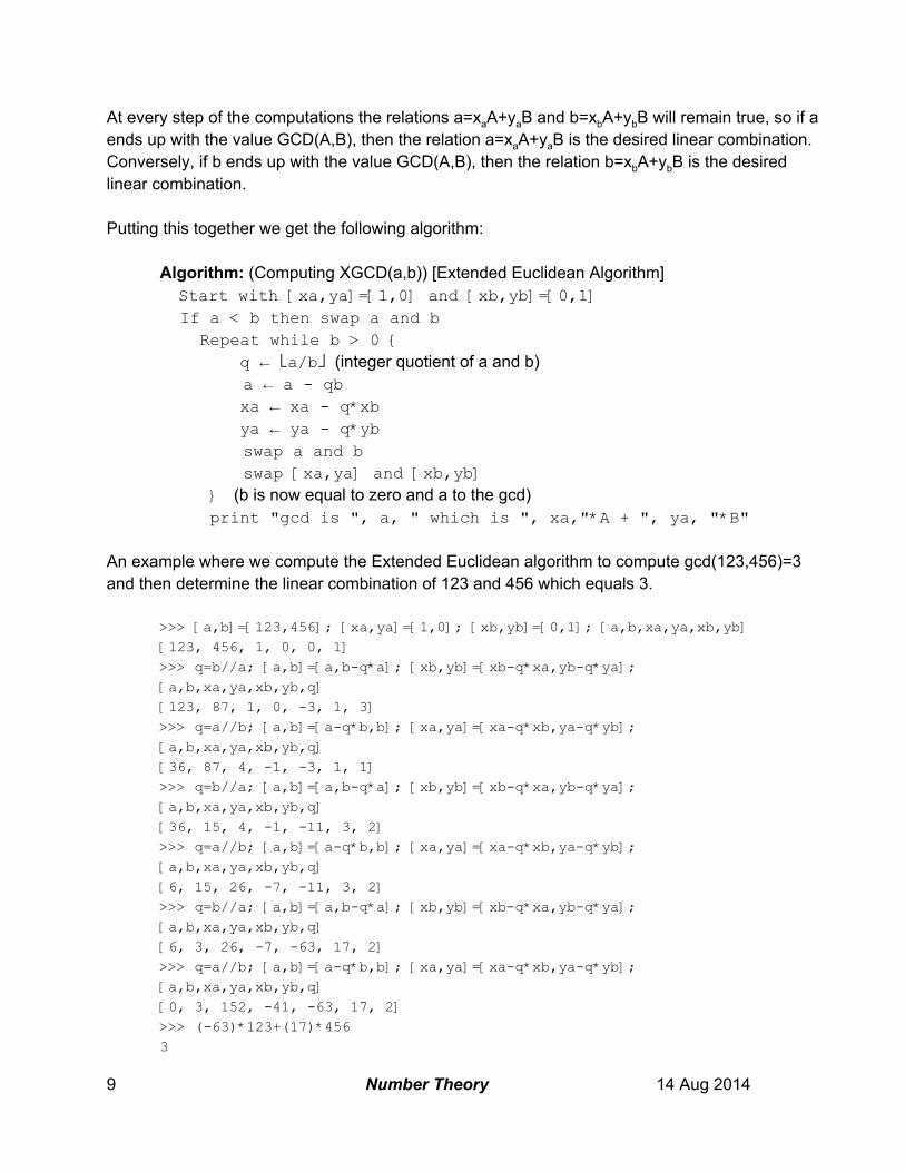
At every step of the computations the relations a=xaA+yaB and b=xbA+ybB will remain true, so if a ends up with the value GCD(A,B), then the relation a=xaA+yaB is the desired linear combination. Conversely, if b ends up with the value GCD(A,B), then the relation b=xbA+ybB is the desired linear combination. Putting this together we get the following algorithm:

Algorithm: (Computing XGCD(a,b)) [Extended Euclidean Algorithm] Start with [xa,ya]=[1,0] and [xb,yb]=[0,1] If a < b then swap a and b Repeat while b > 0 q ← ⌊a/b⌋ (integer quotient of a and b)

a ← a ­ qb xa ← xa ­ q*xb ya ← ya ­ q*yb

swap a and b swap [xa,ya] and [xb,yb]

(b is now equal to zero and a to the gcd) print "gcd is ", a, " which is ", xa,"*A + ", ya, "*B"

An example where we compute the Extended Euclidean algorithm to compute gcd(123,456)=3 and then determine the linear combination of 123 and 456 which equals 3.

>>> [a,b]=[123,456]; [xa,ya]=[1,0]; [xb,yb]=[0,1]; [a,b,xa,ya,xb,yb] [123, 456, 1, 0, 0, 1] >>> q=b//a; [a,b]=[a,b­q*a]; [xb,yb]=[xb­q*xa,yb­q*ya]; [a,b,xa,ya,xb,yb,q] [123, 87, 1, 0, ­3, 1, 3] >>> q=a//b; [a,b]=[a­q*b,b]; [xa,ya]=[xa­q*xb,ya­q*yb]; [a,b,xa,ya,xb,yb,q] [36, 87, 4, ­1, ­3, 1, 1] >>> q=b//a; [a,b]=[a,b­q*a]; [xb,yb]=[xb­q*xa,yb­q*ya]; [a,b,xa,ya,xb,yb,q] [36, 15, 4, ­1, ­11, 3, 2] >>> q=a//b; [a,b]=[a­q*b,b]; [xa,ya]=[xa­q*xb,ya­q*yb]; [a,b,xa,ya,xb,yb,q] [6, 15, 26, ­7, ­11, 3, 2] >>> q=b//a; [a,b]=[a,b­q*a]; [xb,yb]=[xb­q*xa,yb­q*ya]; [a,b,xa,ya,xb,yb,q] [6, 3, 26, ­7, ­63, 17, 2] >>> q=a//b; [a,b]=[a­q*b,b]; [xa,ya]=[xa­q*xb,ya­q*yb]; [a,b,xa,ya,xb,yb,q] [0, 3, 152, ­41, ­63, 17, 2] >>> (­63)*123+(17)*456 3

9 Number Theory 14 Aug 2014

At each step of the computation we can check that a=xa*A+ya*B (where A and B are the original values 123 and 456) and b=xb*A+yb*B. For example, after three steps we see that 15=(­11)*123+(3)*456 (in other words b=xb*A+yb*B). Writing the xgcd in Python as a recursive function (one which calls itself):

>>> def xgcd(a,b,xa=1,ya=0,xb=0,yb=1): ... if a == 0: ... return [b,xb,yb] ... q=b//a ... return xgcd(b­q*a,a,xb­q*xa,yb­q*ya,xa,ya) ... >>> xgcd(123,456) [3, ­63, 17]

Primes

Defn: A prime is an integer greater than 1, whose only positive divisors are itself and 1. So 2 is prime and 3 is prime, but 4 is not prime as it has 2 as a divisor. The primes less than 30 are 2,3,5,7,11,13,17,19, 23, 29.

Counting & Finding Primes

How many primes are there? Will we run out of primes?

Thm: (Euclid, Elements, Book IX, Prop 20) There are an infinite number of primes. proof: Assume not. Thus the set of primes is finite, pi, i = 1, ..., N Consider adding one to the product of these primes: P = ∏i ≤ Npi + 1 This number is strictly greater than any of the primes None of the primes divides it (as pj|∏i ≤ Npi, if pj|∏i ≤ Npi+1, then pj|1) So as no prime divides P it must itself be prime, contradicting our construction of it as larger than any of the (finite number of) primes. Thus our assumption must have been incorrect. ♠

The next step is to find an algorithm which effectively finds primes. This algorithm dates back to Eratosthenes (about 200 BC). The idea is this ­ write down all the integers up to some point: 2 3 4 5 6 7 8 9 10 11 12 13 14 15 16 17 18 19 20 21 22 23 24 25 26 27 28 29. First notice that 2 is prime. Cross out all the even ones larger than 2 (all the composite numbers having 2 as a divisor):

10 Number Theory 14 Aug 2014

2 3 4 5 6 7 8 9 10 11 12 13 14 15 16 17 18 19 20 21 22 23 24 25 26 27 28 29. Now we notice that 3 is prime ­ by now we have checked the only prime smaller than 3, i.e. 2, and seen that 3 is not a multiple of it. Cross out all those divisible by 3 (other than 3): 2 3 4 5 6 7 8 9 10 11 12 13 14 15 16 17 18 19 20 21 22 23 24 25 26 27 28 29. We see that 4 has been crossed out ­ it is a multiple of something and cannot be prime. There is no need to cross out the multiples of 4 as they are already crossed out as multiples of the factors of 4. Thus we continue on to 5, which is not crossed out and hence must be prime (we have crossed out all multiples of smaller primes) Cross out all those divisible by 5 (other than 5): 2 3 4 5 6 7 8 9 10 11 12 13 14 15 16 17 18 19 20 21 22 23 24 25 26 27 28 29. At each step we find the next prime (number not crossed out) publish it as a prime and cross out all of its multiples. So, in this example we see that the numbers 2, 3, 5, 7, 11, 13, 17, 19, 23 and 29 are prime.

Algorithm: (Finding Primes) [Sieve of Eratosthenes] Choose B (the largest number examined) Assert i is prime for all i from 2 to B n ← 2 (set the value of n to 2) while n ≤ B if n is prime print "n is prime" for each i from 2n to B, stepping by n Assert i is not prime else (if n is not prime) n ← n+1 (increment n by one)

A short program in Python which implements the Sieve of Eratosthenes is:

>>> def primes(B): ... isprime = B*[True] # Make a B­long array, all values set to True ... for n in range(2,B): # Step n over 2,3,4,...,B­1 ... if (isprime[n] == True): ... print n," is prime" ... for i in range(2*n,B,n): # Step i over 2n,3n,4n,... ... isprime[i] = False # Multiples of n are not prime ... >>> primes(3000) 2 is prime 3 is prime

11 Number Theory 14 Aug 2014

… 2971 is prime 2999 is prime

If we were to be entirely honest, this algorithm works well if we want to find all the primes less than some bound, but it is inefficient if we want to find a small number of large primes. We will need more background to understand the techniques, but there are methods to determine if a given integer is a prime (or a pseudo­prime, whatever that is). At this point we have defined the primes, we know that there are an infinite number of them and we know how to find them. It might be nice to have a better handle on how many primes there are less than some bound. How many primes are there less than 100? How many less than 1000? How many less than a million … a billion … etc? A brute force way to do this is to modify the Sieve of Eratosthenes to just count the primes, rather than printing them out. [Add a second line numprimes=0, replace the line print n,” is prime” with the line numprimes = numprimes + 1, and add a final line return numprimes, indented the same amount as the second line.] There are 10 primes less than 30, 25 primes less than 100, 168 less than 1000, 1229 less than 10000, 9592 less than 100000 and 78498 less than a million. So while the number of primes is steadily growing, their density seems to be decreasing. For convenience we denote this count (x).π

Def: The number of primes less than or equal to some bound B is called the prime pi function, denoted (B).π

Looking at counts of the number of primes less than some bound B lead Legendre [1796] and Gauss [1800] to conjecture that its value was approximately (x) x/log(x), which was provenπ ~ almost a century later:

Thm: (Prime Number Theorem) The number of primes less than or equal to x is asymptotically equal to x/log(x).

This allows us to make estimates of the number of primes less than some bound. An application of this is that we can estimate the likelihood that a randomly chosen number of a particular size is prime. For instance, if we randomly choose a 100­bit (about 30­digit) number, the likelihood that it will be prime is about 1/log(2100) = 0.0144 (or about one in 70). Of course, if we really wanted a prime we could easily improve our odds by insisting that it be odd, etc.

Unique Factorization

We have defined primality conventionally in terms of the divisors. A property which turns out to be equivalent is the following:

12 Number Theory 14 Aug 2014

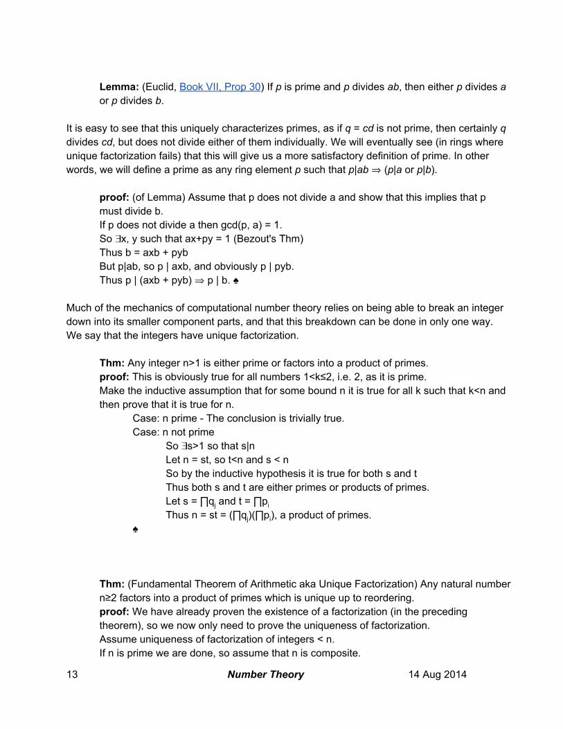
Lemma: (Euclid, Book VII, Prop 30) If p is prime and p divides ab, then either p divides a or p divides b.

It is easy to see that this uniquely characterizes primes, as if q = cd is not prime, then certainly q divides cd, but does not divide either of them individually. We will eventually see (in rings where unique factorization fails) that this will give us a more satisfactory definition of prime. In other words, we will define a prime as any ring element p such that p|ab ⇒ (p|a or p|b).

proof: (of Lemma) Assume that p does not divide a and show that this implies that p must divide b. If p does not divide a then gcd(p, a) = 1. So ∃x, y such that ax+py = 1 (Bezout's Thm) Thus b = axb + pyb But p|ab, so p | axb, and obviously p | pyb. Thus p | (axb + pyb) ⇒ p | b. ♠

Much of the mechanics of computational number theory relies on being able to break an integer down into its smaller component parts, and that this breakdown can be done in only one way. We say that the integers have unique factorization.

Thm: Any integer n>1 is either prime or factors into a product of primes. proof: This is obviously true for all numbers 1<k≤2, i.e. 2, as it is prime. Make the inductive assumption that for some bound n it is true for all k such that k<n and then prove that it is true for n.

Case: n prime ­ The conclusion is trivially true. Case: n not prime

So ∃s>1 so that s|n Let n = st, so t<n and s < n So by the inductive hypothesis it is true for both s and t Thus both s and t are either primes or products of primes. Let s = ∏qj and t = ∏pi Thus n = st = (∏qj)(∏pi), a product of primes.

♠

Thm: (Fundamental Theorem of Arithmetic aka Unique Factorization) Any natural number n≥2 factors into a product of primes which is unique up to reordering. proof: We have already proven the existence of a factorization (in the preceding theorem), so we now only need to prove the uniqueness of factorization. Assume uniqueness of factorization of integers < n. If n is prime we are done, so assume that n is composite.

13 Number Theory 14 Aug 2014

Suppose n has two factorizations: n = ∏ pi = ∏ qj So we need to prove that the two sequences pi and qj are equal up to reordering. As p1 | n we have p1 | ∏ qj. By repeatedly applying the Lemma proved in the preceding section we see that there is some index k such that p1 | qk (and hence p1 = qk) So n/p1 = n/qk. But n/p1 < n so by the inductive hypothesis it must have a unique factorization. Thus n/p1 = n/qk has the unique factorization ∏i≠1pi. Thus the sequences pi: i≠1 and qj: j≠k are equal up to reordering. ♠

It is easy to take the unique factorization property for granted, but with more experience we will see that this gift is not something which had to happen. Among the similar “integers” that are dealt with in the advanced topics of number theory there are examples with unique factorization (for example the Gaussian integers, Z[i]) and conversely there are examples where unique factorization fails (for example Z[√­5], where the otherwise perfectly well behaved integer 6 has as prime factorizations both 6 = (2)(3) and a second one 6 = (­1)(1+√­5)(1­√­5)).

Congruences

We have worked up to now with the somewhat simple concept of divisibility, so we can talk about all the multiples of some number ­ for instance the set of multiples of 5, ...,­10,­5,0,5,10,15,.... We need a more refined language, one which allows us to talk about all the integers which are two greater than a multiple of 5, ...,­8,­3,2,7,12,17, .... This is the language of congruences:

Def: [Gauss] We say that integer a is congruent to b mod N (denoted a b(mod N)) iff≡ there is some integer k such that a­b=kN.

With this definition we can talk about the set of all integers which are congruent to each other. Thus ...,­10,­5,0,5,10,15,... is the set of all integers which are congruent to 0 mod 5, and ...,­8,­3,2,7,12,17, ... is the set of all integers which are congruent to 7 mod 5 (equally, we could say that it is the set of integers which are congruent to 2 mod 5). We will eventually want to perform arithmetic with these sets, defining a way of “adding”, “multiplying” and sometimes “dividing” them. If we need to be very careful we can refer to these infinite sets with a new notation, perhaps referring to the set of integers with are three more than a multiple of five as [3]5. We will start our discussion with this clumsy notation, but very quickly we will let ourselves get sloppy and just refer to [3]5 as 3.

Def: Given some modulus N, the set of subsets of the integers which are equivalent to each other are referred to as the integers mod N and denoted ZN.

14 Number Theory 14 Aug 2014

Thus the set of integers mod 5 is the set Z5 = [0]5, [1]5, [2]5, [3]5, [4]5, where [0]5=...,­10,­5,0,5,10,15,..., [1]5=...,­9,­4,1,6,11,16,..., etc. This is an example of a more general construction ­ one of equivalence relations and equivalence classes. If some set S (in our case the integers Z) has a relation (in our case congruence mod some N) which is (i) Reflexive (ie a a), (ii) Symmetric (ie if a ~ ~ ~b then b a), and (iii) Transitive (ie if a b and b c, then a c), then the set is divided into subsets whose elements are equivalent ~ ~ ~ ~ to each other. This subsets are called equivalence classes. The set of equivalence classes can then be manipulated and in some cases (as in ours) can have arithmetic operations on them.

Modular Arithmetic

We will work with the example of arithmetic mod 6, dividing the integers into the six sets: [0]6 = ...,­12,­6,0,6,12,18,... [1]6 = ...,­11,­5,1,7,13,19,... [2]6 = ...,­10,­4,2,8,14,20,... [3]6 = ...,­9,­3,3,9,15,21,... [4]6 = ...,­8,­2,4,10,16,22,... [5]6 = ...,­7,­1,5,11,17,23,...

In order to add two of these sets we form all possible sums of elements of the two sets. Thus the sum of [2]6 and [3]6 includes the elements ­10+21 = 11, 2+3 = 5, 14+15 = 39, etc. As we don’t have the time to compute all possible sums, perhaps we can do this symbolically. Note that [2]6 is the set of elements 2+6i | i Z and [3]6 is the set of elements 3+6k | k Z. Thus we∈ ∈ can compute their elementwise sum as [2]6 + [3]6 is the set of elements (2+6i) + (3+6k)| i,k Z,∈ which can be rewritten as (2+3) + (6(i+k)) | i,k Z = 5 + (6(i+k)) | i,k Z, in other words five∈ ∈ more than all possible multiples of six, or [5]6. Thus [2]6 + [3]6 = [5]6. A similar computation yields a slightly less obvious result:

[3]6 + [4]6 = 3+6k | k Z + 4+6j | j Z∈ ∈ = (3+6k) + (4+6j) | k,j Z∈ = (3+4) + (6(k+j)) | k,j Z∈ = 7 + (6(k+j)) | k,j Z, but with a little rearranging we get∈ = 1 + (6(k+j+1)) | k,j Z, which is one more than all multiples of six, so [1]6.∈ Thus [3]6 + [4]6 = [1]6.

Note that we referred to this last result as [1]6 rather than the more obvious [7]6. Both names are correct, but it will prove convenient to always refer to one of these sets by the smallest non­negative element of it. Because of the division algorithm we know that there is such an element, that it is unique and that it is less than 6. In fact, the division algorithm also assures us that it is easy to find, given any representative of the set. From now on, we will use only this set of reduced representatives.

15 Number Theory 14 Aug 2014

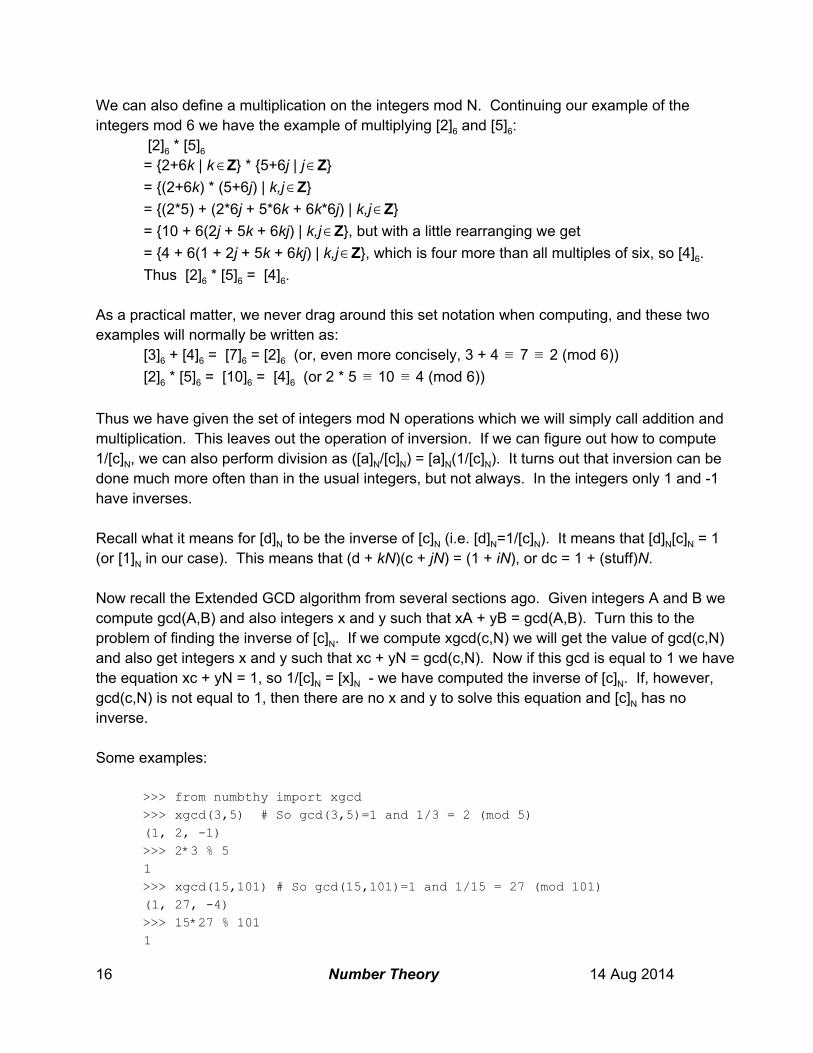
We can also define a multiplication on the integers mod N. Continuing our example of the integers mod 6 we have the example of multiplying [2]6 and [5]6:

[2]6 * [5]6 = 2+6k | k Z * 5+6j | j Z∈ ∈ = (2+6k) * (5+6j) | k,j Z∈ = (2*5) + (2*6j + 5*6k + 6k*6j) | k,j Z∈ = 10 + 6(2j + 5k + 6kj) | k,j Z, but with a little rearranging we get∈ = 4 + 6(1 + 2j + 5k + 6kj) | k,j Z, which is four more than all multiples of six, so [4]6.∈ Thus [2]6 * [5]6 = [4]6.

As a practical matter, we never drag around this set notation when computing, and these two examples will normally be written as:

[3]6 + [4]6 = [7]6 = [2]6 (or, even more concisely, 3 + 4 7 2 (mod 6))≡ ≡ [2]6 * [5]6 = [10]6 = [4]6 (or 2 * 5 10 4 (mod 6))≡ ≡

Thus we have given the set of integers mod N operations which we will simply call addition and multiplication. This leaves out the operation of inversion. If we can figure out how to compute 1/[c]N, we can also perform division as ([a]N/[c]N) = [a]N(1/[c]N). It turns out that inversion can be done much more often than in the usual integers, but not always. In the integers only 1 and ­1 have inverses. Recall what it means for [d]N to be the inverse of [c]N (i.e. [d]N=1/[c]N). It means that [d]N[c]N = 1 (or [1]N in our case). This means that (d + kN)(c + jN) = (1 + iN), or dc = 1 + (stuff)N. Now recall the Extended GCD algorithm from several sections ago. Given integers A and B we compute gcd(A,B) and also integers x and y such that xA + yB = gcd(A,B). Turn this to the problem of finding the inverse of [c]N. If we compute xgcd(c,N) we will get the value of gcd(c,N) and also get integers x and y such that xc + yN = gcd(c,N). Now if this gcd is equal to 1 we have the equation xc + yN = 1, so 1/[c]N = [x]N ­ we have computed the inverse of [c]N. If, however, gcd(c,N) is not equal to 1, then there are no x and y to solve this equation and [c]N has no inverse. Some examples:

>>> from numbthy import xgcd >>> xgcd(3,5) # So gcd(3,5)=1 and 1/3 = 2 (mod 5) (1, 2, ­1) >>> 2*3 % 5 1 >>> xgcd(15,101) # So gcd(15,101)=1 and 1/15 = 27 (mod 101) (1, 27, ­4) >>> 15*27 % 101 1

16 Number Theory 14 Aug 2014

>>> xgcd(6,14) # So gcd(6,14)=2, not 1, and 6 has no inverse (mod 14) [2, ­2, 1]

Thus 1/[3]5 = [2]5 and 1/[15]101 = [27]101, but there is no inverse for [6]14 as the gcd(6,14) is not equal to 1. With a little thought we see that if the modulus N is prime (so every integer between 1 and N­1 is coprime with it) then every element but [0]N has an inverse. Conversely, if N is composite, then some of the integers between 1 and N­1 will have a gcd other than 1 with N, and will not have an inverse.

Def: Given a modulus N, the set of integers mod N which are coprime to N (and hence have inverses) is called the group of units mod N and denoted ZN

*. Note that while we can add and multiply and still stay in the integers mod N, ZN

*, we can only multiply in the group of units mod N, ZN

* ­ addition is not guaranteed to produce a result still in the group. We have outlined one approach to making sense of this arithmetic of congruences ­ viewing each element as an infinite set. This approach extends well to more general cases in abstract algebra. A second way of describing what we are doing is to perform the usual arithmetic operations, but allow any multiple of the modulus to be discarded. A little thought needs to be expended in showing that the final result does not depend on what multiples are discarded and when during the computation, but the result of both approaches is the same.

Fast Exponentiation

When computing a power of a number with a finite modulus there are efficient ways to do it and inefficient ways to do it. In this section we will outline a commonly used efficient method which has the curious name "the Russian Peasant algorithm". The most obvious way to compute 1210 (mod 23) is to multiply 12 a total of nine times, reducing the result mod 23 at each step. A more efficient method which takes only four multiplications is accomplished by first noting that: 122=6 (mod 23) 124=62=13 (mod 23) 128=132=8 (mod 23) We have now performed three squarings and, by noting that the exponent breaks into powers of 2 as 10=8+2, we can rewrite our computation: 1210=12(8+2)

=128*122

=8*6=2(mod 23)

17 Number Theory 14 Aug 2014

So our algorithm consists of writing the exponent as sums of powers of two. (This can be done by writing it as a number base 2 and reading off successive digits ­ eg 1010=10102.) Now we multiply successive squares of the base number for each digit of the exponent which is a "1". The following short program will allow you to compute examples of the Russian Peasant method for exponentiation: Here we are computing the value of be(mod N). We will be looping over successive bits of the exponent e, so we will have log2(e) loops. Here we denote the ith bit of e as e[i].

Algorithm: (Russian Peasant Exponentiation) accum = 1 s = b (so s=b2^0) for i=0 to log2(e) do:

s ← s2 (mod N) (so s=b2^i) if (e[i] == 1) then:

accum ← accum*s (mod N) end if

end for print accum

Thinking about the algorithm this way, we can estimate how much work is involved. For anything but the smallest numbers, most of the work will be in the modular multiplies and the modular squarings. The total number of bits in the exponent is log2(e) ­ we can call this value k. There will be k squarings in the computation. The number of multiplications will be equal to the number of bits in e which are 1 in its binary representation, which ranges between 1 and k, but is almost always close to k/2 for random exponents. Thus the total work involved in the algorithm is roughly kS+kM/2, where S and M are the work of a single squaring and multiply, respectively. This is the algorithm generally used for modular exponentiation. The general outline of it is also used to compute in elliptic curves, and many other contexts, so this is a very important algorithm. But this is not guaranteed to be the best approach for any problem. There is a long literature on the question of finding the best addition chain for a given problem. An important example where it makes a big difference is in computing the value of b(2190­262) (mod N). We could use the above algorithm at a cost of 189S+127M, or use a more carefully crafted algorithm which takes only 189S+7M though. (The context is in the US government's elliptic curve e­signature algorithm.) Recent surveys of methods of efficiently computing a modular power are [Gord98] and [Bern02].

In Python there is already a command which performs this algorithm ­ the pow function. It is worth the effort to write and look at some code which implements this algorithm:

>>> def powmod(b,e,n): ... accum = 1; i = 0; bpow2 = b ... while ((e>>i)>0): # For each bit in the exponent e ... if((e>>i) & 1): # If the ith bit in e is a 1

18 Number Theory 14 Aug 2014

... accum = (accum*bpow2) % n

... bpow2 = (bpow2*bpow2) % n

... i=i+1

... return accum >>> powmod(2,75,101) 91 >>> pow(2,75,101) # The built­in function 91

Diffie-Hellman Key Agreement

All public key algorithms rely on some computation which is easy to perform, but whose inverse is very difficult to perform. The Diffie­Hellman key agreement algorithm depends on the fact (seen in the previous section) that, given g, e and N, computing the modular exponentiation ge (mod N) is very easy and quick with the Russian Peasant algorithm. An inverse of this operation is referred to as the discrete logarithm operation. Given g, N and a, it is very difficult to find an exponent e such that ge (mod N) .

Assumption: (Discrete Logarithm) Given g, N and a, it is difficult (impractical) to find an exponent e such that ge (mod N) (if such an e exists).

The context of the key agreement algorithm is this: Alice and Bob start with no shared secret and no secure channel that they can share a secret over. The only channel that they can communicate over is listened to by their opponent Eve (for eavesdropper). Yet, somehow at the end of the process Alice and Bob, using only the channel listened to by Eve, will be able to share a secret value that they both know, but that Eve doesn’t know.

Algorithm: (Diffie­Hellman Key Agreement) A and/or B:

Choose prime p and element g Publish p, g as public parameters (known to them and also to Eve)

A: Choose rA, a secret value Compute RA := grA (mod p) Send RA to B (Presumably intercepted by Eve)

B: Choose rB, a secret value Compute RB := grB (mod p) Send RB to A (Presumably intercepted by Eve)

A: Compute S=RB

rA, the shared secret B:

19 Number Theory 14 Aug 2014

Compute S=RArB, the shared secret

A shared secret is only useful if A and B come up with the same shared secret. We see that for A the value is computed as S=RB

rA=(grB)rA=grBrA (which is true even though A doesn’t know the value of rB) and for B the value is computed as S=RA

rB=(grA)rB=grArB. From the usual properties of exponents we know that grArB=grBrA, so both Alice and Bob now have the same secret. Even though Eve has presumably seen the values of RA and RB, and knows that they were computed as grA and grB, unless she can solve the discrete logarithm problem she can’t recover either rA or rB and can’t compute S. (Eve’s problem is actually subtly different, but equivalent to the discrete logarithm problem in many cases.) An example (with ridiculously small parameters) is:

>>> # Alice and Bob agree publicly on the parameters >>> p = 101 # A large prime number >>> g = 2 # An integer mod p >>> # Alice generates a random number >>> xA = 37 >>> # Alice computes her public value >>> yA = pow(g,xA,p); yA # Compute g**xA (mod p) efficiently 55 >>> xB = 15 # Bob chooses a random number >>> yB = pow(g,xB,p); yB # Bob computes his public g**xB (mod p) efficiently 44 >>> # Alice sends yA to Bob and Bob sends yB to Alice >>> pow(yB,xA,p) # Alice computes yB**xA (mod p) 69 >>> pow(yA,xB,p) # Bob computes yA**xB (mod p) 69

An interesting point about the Diffie­Hellman key agreement was that it wasn’t developed first by Diffie and Hellman. The outside development was by Diffie and Hellman, using early work by Merkle, and published in 1976. In 1973 Malcolm Williamson, working at GCHQ, developed the same algorithm, although this fact was kept secret until it was declassified in 1997.

Chinese Remainder Theorem

Thm: If p and q are coprime and we have the two relations x ≡ a (mod p) and x ≡ b (mod q), then x ≡ ak + bl (mod pq), where k = q(q­1 (mod p)) and l = p(p­1 (mod q)). proof: write out and observe ­ need some words on uniqueness

Example: x ≡ 3 (mod 5)

20 Number Theory 14 Aug 2014

x ≡ 2 (mod 9) k = 9(9­1 (mod 5)) = (9)(4) = 36 l = 5(5­1 (mod 9)) = (5)(2) = 10 So x ≡ (3)(36) + (2)(10) = 108+20 ≡ 38 (mod 45)

Note that while p and q need to be coprime, they do not need to be prime. The value of this result is that can allow some large problems to be broken into numerous small problems, and then the answers to the small problems can be put together to reconstruct the answer of the large problem. A method of breaking up a problem over a prime power modulus is Hensel's Lemma, which we might get to later. Observations on how this can be applied to Diffie­Hellman if Alice and Bob choose a modulus p such that p­1 has many small factors.

Fermat’s Little Theorem

Here is a result which dates back at least to 1640 when Fermat stated in a letter to a friend that if p is prime and a is not a multiple of p, then p divides a(p­1)­1. As usual, Fermat provided no proof, and it wasn't until 1736 that the first proof was published by Euler. Some example computations are useful before we dive in and prove it.

p=7 and a=2: 27­1 = 64, so 26­1 = 63, which is divisible by 7. p=7 and a=5: 57­1 = 15625, so 56­1 = 15624, which is divisible by 7.

These numbers are becoming unpleasantly large to compute with, so we find it useful to recast Fermat's assertion into the language of congruences and modular arithmetic. In this form it becomes if p is prime and a is not congruent to 0 (mod p), then a(p­1) = 1 (mod p). Now we are in the position (together with the efficient method for modular exponentiation we just learned) to do some larger examples.

p=17 and a=5: 517­1 = 1 (mod 17) This is particularly simple to compute as 516 = ((((52)2)2)2) = (((252)2)2) = (((132)2)2) = ((1692)2) = ((­12)2) = (12) = 1 (mod 17)

p=101 and a=3: 3101­1 = 1 (mod 100)

p=99 and a=5: 599­1 = 70 (mod 99) (but of course 99 isn't prime, so this theorem doesn't even apply.)

p=341: note that 341=(11)(31), so it isn't prime a=2: 2341­1 = 1 (mod 341) a=3: 3341­1 = 56 (mod 341)

21 Number Theory 14 Aug 2014

So sometimes (but rather rarely) the converse doesn't hold ­ there are non­primes p and bases a for which a(p­1) = 1 (mod p). We call these cases "pseudo­primes" for reasons that will be made clearer in the next section.

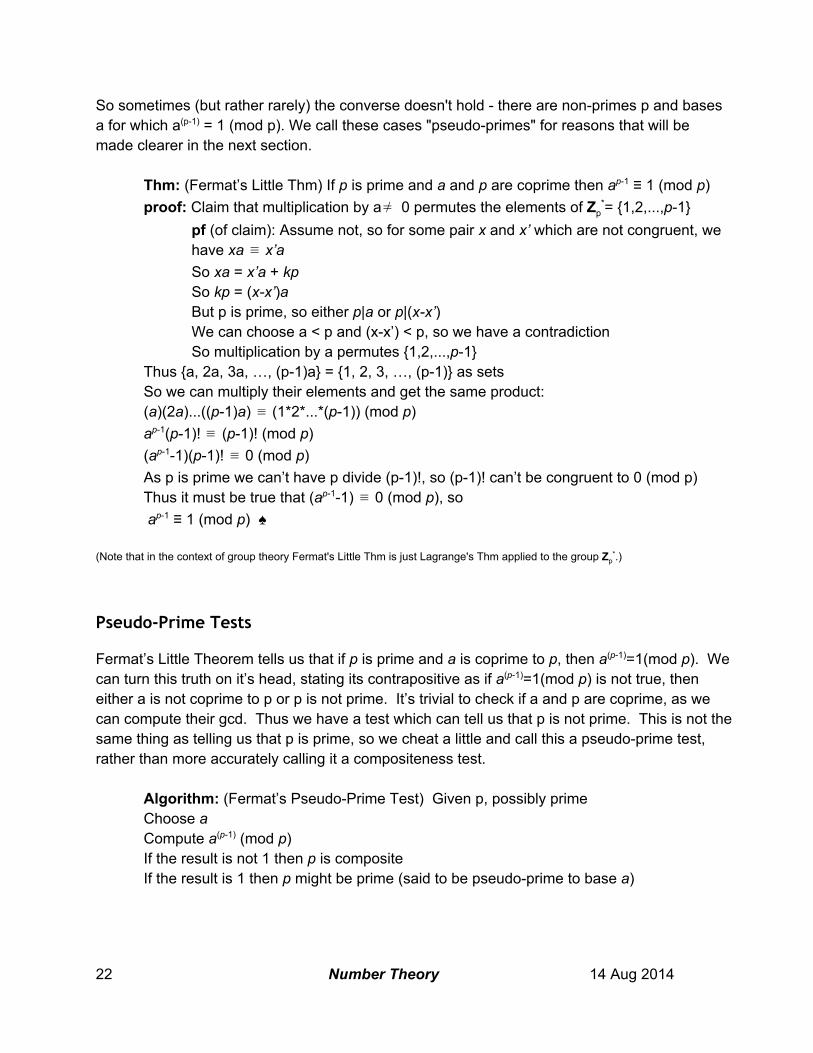
Thm: (Fermat’s Little Thm) If p is prime and a and p are coprime then ap­1 ≡ 1 (mod p) proof: Claim that multiplication by a 0 permutes the elements of Zp

*= 1,2,...,p­1=/ pf (of claim): Assume not, so for some pair x and x’ which are not congruent, we have xa x’a≡ So xa = x’a + kp So kp = (x­x’)a But p is prime, so either p|a or p|(x­x’) We can choose a < p and (x­x’) < p, so we have a contradiction So multiplication by a permutes 1,2,...,p­1

Thus a, 2a, 3a, …, (p­1)a = 1, 2, 3, …, (p­1) as sets So we can multiply their elements and get the same product: (a)(2a)...((p­1)a) (1*2*...*(p­1)) (mod p)≡ ap­1(p­1)! (p­1)! (mod p)≡ (ap­1­1)(p­1)! 0 (mod p)≡ As p is prime we can’t have p divide (p­1)!, so (p­1)! can’t be congruent to 0 (mod p) Thus it must be true that (ap­1­1) 0 (mod p), so≡ ap­1 ≡ 1 (mod p) ♠

(Note that in the context of group theory Fermat's Little Thm is just Lagrange's Thm applied to the group Zp

*.)

Pseudo-Prime Tests

Fermat’s Little Theorem tells us that if p is prime and a is coprime to p, then a(p­1)=1(mod p). We can turn this truth on it’s head, stating its contrapositive as if a(p­1)=1(mod p) is not true, then either a is not coprime to p or p is not prime. It’s trivial to check if a and p are coprime, as we can compute their gcd. Thus we have a test which can tell us that p is not prime. This is not the same thing as telling us that p is prime, so we cheat a little and call this a pseudo­prime test, rather than more accurately calling it a compositeness test.

Algorithm: (Fermat’s Pseudo­Prime Test) Given p, possibly prime Choose a Compute a(p­1) (mod p) If the result is not 1 then p is composite If the result is 1 then p might be prime (said to be pseudo­prime to base a)

22 Number Theory 14 Aug 2014

If p passes this test for a number of values of a we have some confidence that it is prime. If p passes enough pseudo­prime tests (usually more sophisticated tests than the Fermat pseudoprime test) we often say that p is an industrial­grade prime. Consider some examples of applying this test:

Is 13 prime? 2(13­1) 1 (mod 13) ­ so far so good≡ 3(13­1) 1 (mod 13) ­ still looking good≡ So it looks as though 13 is prime

Is 35 prime? 2(35­1) 9 (mod 35) ­ so 35 is definitely not prime≡

Is 1237 prime? 2(1237­1) 1 (mod 1237) ­ so far so good≡ 3(1237­1) 1 (mod 1237) ­ looking pretty good≡ 75(1237­1) 1 (mod 1237) ­ pretty good evidence so far≡ 1237 is prime

Is 1387 prime? 2(1387­1) 1 (mod 1387) ­ so far so good≡ 3(1387­1) 875 (mod 1387) ­ oops≡ So 1387 must not be prime (in fact 1387 = (19)(73))

Recall that these tests are easily performed in Python with commands such as:

>>> pow(3,1386,1387) 875

The integer 1387, because it “fools” the base 2 is called a pseudoprime base 2. Pseudoprimes are somewhat rare, but even rarer are integers such as 1729 = (7)(13)(19), which are pseudoprimes to every base to which they are coprime. These unusual numbers are called Carmichael numbers.

Euler’s -Function φ

Def: A unit in ZN is an integer n which has an inverse mod N.

Thus mod 12 the units are 1, 5, 7 and 11. All the other integers 0,2,3,4,6,8,9,10 are not coprime to 12. Recall that we use the extended GCD algorithm to compute their inverses. We observe that the units are closed under multiplication as (ab)­1 = b­1a­1. There always is at least one unit, as 1 is always a unit. With these observations we say that the units form a group under multiplication, and talk about the group of units mod N, ZN*. This use of the word group comes from abstract algebra, where it has a much more general use. The group of units, ZN*, from number theory was one of the examples which motivated the more general definition of group.

23 Number Theory 14 Aug 2014

Euler’s -Function φ

Def: (The Euler φ Function) φ(N) (also called the totient function) is defined as the number of positive integers a < N such that gcd(a, N) = 1.

Equivalently, φ(N) is the number of elements in the group of units mod N. Thm: (Computing Euler’s φ­Function)

φ(pe) = (p­1)pe­1 for prime p φ(nm) = φ(n) φ(m) if gcd(n,m) = 1

Examples: φ(15) = φ(3) φ(5) = (3­1)(5­1) = 8. Note that φ(15) = #n: gcd(n,15) = 1 =

#1,2,4,7,8,11,13,14 = 8. φ(16) = φ(24) = (2­1)2(4­1) = 8, and φ(16) = #n: gcd(n,16) = 1 = #1,3,5,7,9,11,13,15 = 8. φ(123440) = φ((23)(5)(1543)) = ((2­1)2(3­1))(5­1)(1543­1) = 49344

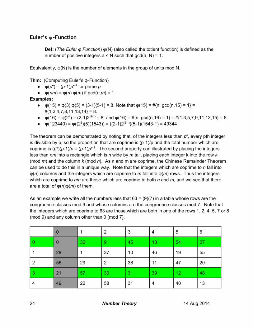
The theorem can be demonstrated by noting that, of the integers less than pe, every pth integer is divisible by p, so the proportion that are coprime is (p­1)/p and the total number which are coprime is (pe)(p­1)/p = (p­1)pe­1. The second property can illustrated by placing the integers less than nm into a rectangle which is n wide by m tall, placing each integer k into the row k (mod m) and the column k (mod n). As n and m are coprime, the Chinese Remainder Theorem can be used to do this in a unique way. Note that the integers which are coprime to n fall into φ(n) columns and the integers which are coprime to m fall into φ(m) rows. Thus the integers which are coprime to nm are those which are coprime to both n and m, and we see that there are a total of φ(n)φ(m) of them. As an example we write all the numbers less that 63 = (9)(7) in a table whose rows are the congruence classes mod 9 and whose columns are the congruence classes mod 7. Note that the integers which are coprime to 63 are those which are both in one of the rows 1, 2, 4, 5, 7 or 8 (mod 9) and any column other than 0 (mod 7).

0 1 2 3 4 5 6

0 0 36 9 45 18 54 27

1 28 1 37 10 46 19 55

2 56 29 2 38 11 47 20

3 21 57 30 3 39 12 48

4 49 22 58 31 4 40 13

24 Number Theory 14 Aug 2014

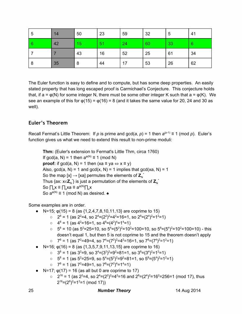
5 14 50 23 59 32 5 41

6 42 15 51 24 60 33 6

7 7 43 16 52 25 61 34

8 35 8 44 17 53 26 62

The Euler function is easy to define and to compute, but has some deep properties. An easily stated property that has long escaped proof is Carmichael’s Conjecture. This conjecture holds that, if a = φ(N) for some integer N, there must be some other integer K such that a = φ(K). We see an example of this for φ(15) = φ(16) = 8 (and it takes the same value for 20, 24 and 30 as well).

Euler’s Theorem

Recall Fermat’s Little Theorem: If p is prime and gcd(a, p) = 1 then a(p­1) ≡ 1 (mod p). Euler’s function gives us what we need to extend this result to non­prime moduli:

Thm: (Euler's extension to Fermat's Little Thm, circa 1760) If gcd(a, N) = 1 then aφ(N) ≡ 1 (mod N) proof: if gcd(a, N) = 1 then (xa ≡ ya ⇔ x ≡ y) Also, gcd(a, N) = 1 and gcd(x, N) = 1 implies that gcd(xa, N) = 1 So the map [x] → [xa] permutes the elements of ZN

* Thus ax: x∈ZN

* is just a permutation of the elements of ZN*

So ∏xx ≡ ∏xxa ≡ aφ(N)∏xx So aφ(N) ≡ 1 (mod N) as desired. ♠

Some examples are in order.

N=15; φ(15) = 8 (as 1,2,4,7,8,10,11,13 are coprime to 15) 28 = 1 (as 22=4, so 24=(22)2=42=16=1, so 28=(24)2=12=1) 48 = 1 (as 42=16=1, so 48=(42)4=14=1) 58 = 10 (as 52=25=10, so 54=(52)2=102=100=10, so 58=(54)2=102=100=10) ­ this

doesn’t equal 1, but then 5 is not coprime to 15 and the theorem doesn’t apply 78 = 1 (as 72=49=4, so 74=(72)2=42=16=1, so 78=(74)2=12=1)

N=16; φ(16) = 8 (as 1,3,5,7,9,11,13,15 are coprime to 16) 38 = 1 (as 32=9, so 34=(32)2=92=81=1, so 38=(34)2=12=1) 58 = 1 (as 52=25=9, so 54=(52)2=92=81=1, so 58=(54)2=12=1) 78 = 1 (as 72=49=1, so 78=(72)4=14=1)

N=17; φ(17) = 16 (as all but 0 are coprime to 17) 216 = 1 (as 22=4, so 24=(22)2=42=16 and 28=(24)2=162=256=1 (mod 17), thus

216=(28)2=12=1 (mod 17))

25 Number Theory 14 Aug 2014

316 = 1 (as 32=9, so 34=(32)2=92=81=13, 38=(34)2=132=169=16, 316=(38)2=162=256=1 (mod 17))

N=21; φ(21) = 12 (as 1,2,4,5,8,10,11,13,16,17,19,20 are coprime to 21) 212 = 1 (as 22=4, so 24=(22)2=42=16 and 28=(24)2=162=256=4 (mod 21), thus

212=(28)(24)=(4)(16)=64=1 (mod 21)) An observation we can make in these examples is that, while aφ(N) ≡ 1 (mod N), sometimes ae=1 for smaller exponents e. We could ask when this is the case, and if there are any elements for which it is never the case. This is the question of primitive elements, which we will deal with later. In the interim, we can at least make a definition which will allow us to talk about the question:

Def: If a and N are coprime, then the order of a mod N (denoted o(a)(mod N)) is the smallest non­zero exponent e such that ae = 1 (mod N).

Clearly Euler’s Theorem (and Fermat’s Little Theorem in the prime modulus case) puts some conditions on the possible values the order of an integer mod N can take.

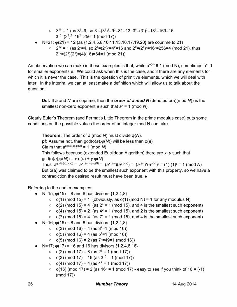
Theorem: The order of a (mod N) must divide φ(N). pf: Assume not, then gcd(o(a),φ(N)) will be less than o(a) Claim that agcd(o(a),φ(N)) = 1 (mod N) This follows because (extended Euclidean Algorithm) there are x, y such that gcd(o(a),φ(N)) = x o(a) + y φ(N) Thus agcd(o(a),φ(N)) = ax o(a) + y φ(N) = (ax o(a))(ay φ(N)) = (ao(a))x(aφ(N))y = (1)x(1)y = 1 (mod N) But o(a) was claimed to be the smallest such exponent with this property, so we have a contradiction the desired result must have been true. ♠

Referring to the earlier examples:

N=15; φ(15) = 8 and 8 has divisors 1,2,4,8 o(1) (mod 15) = 1 (obviously, as o(1) (mod N) = 1 for any modulus N) o(2) (mod 15) = 4 (as 24 = 1 (mod 15), and 4 is the smallest such exponent) o(4) (mod 15) = 2 (as 42 = 1 (mod 15), and 2 is the smallest such exponent) o(7) (mod 15) = 4 (as 74 = 1 (mod 15), and 4 is the smallest such exponent)

N=16; φ(16) = 8 and 8 has divisors 1,2,4,8 o(3) (mod 16) = 4 (as 34=1 (mod 16)) o(5) (mod 16) = 4 (as 54=1 (mod 16)) o(5) (mod 16) = 2 (as 72=49=1 (mod 16))

N=17; φ(17) = 16 and 16 has divisors 1,2,4,8,16 o(2) (mod 17) = 8 (as 28 = 1 (mod 17)) o(3) (mod 17) = 16 (as 316 = 1 (mod 17)) o(4) (mod 17) = 4 (as 44 = 1 (mod 17)) o(16) (mod 17) = 2 (as 162 = 1 (mod 17) ­ easy to see if you think of 16 = (­1)

(mod 17))

26 Number Theory 14 Aug 2014

N=21; φ(21) = 12 and 12 has divisors 1,2,3,4,6,12 o(2) (mod 21) = 6 (as 26 = 1 (mod 21), but 22=4 and 23=8, so checking only

divisors, 6 is the smallest candidate) o(4) (mod 21) = 3 (as 43 = 1 (mod 21), but 42=16) o(5) (mod 21) = 6 (as 56 = 1 (mod 21), but 52=25=4 and 53=125=20) o(8) (mod 21) = 2 (as 82 = 64 = 1 (mod 21))

If Euler’s Theorem limits the values that the order can take on, an interesting question is what values actually appear. We will give a partial answer later ­ giving conditions for when some integer mod N has order φ(N).

RSA Encryption

The Rivest­Shamir­Adleman encryption algorithm relies on what is called a trapdoor one­way function. Given P, e and N, computing the modular exponentiation Pe (mod N) is very easy and quick using fast exponentiation. An inverse is to take the result of this operation, called C (for ciphertext) and recover the original P (for plaintext). This would be a very easy operation if you could just take the eth root of C mod N. But taking a root mod N generally requires having a factorization of N. With this factorization it is easy to find an exponent d (for decrypt) such that computing the dth power is equivalent to taking the eth root. Thus decrypting RSA is equivalent to the factoring problem.

Assumption: (Factoring) Given an integer N which you know to be be product of two large prime factors, it is difficult (impractical) to find these factors.

The context of the key agreement algorithm is this: Alice and Bob start with no shared secret and no secure channel that they can share a secret over. The only channel that they can communicate over is listened to by their opponent Eve (for eavesdropper). RSA allows Bob to encrypt a message which only Alice can decrypt.

Algorithm: (RSA Encryption) A:

Choose (secret) primes p and q Choose (public) exponent e (which must be coprime to both p and q) Compute (public) modulus N=pq Compute (secret) ) φ(N) = (p­1)(q­1) and d = e(­1) (mod φ(N)) Publish N, e as public parameters (known to them and also to Eve)

B: Given a (secret) plaintext message P he wants to send to Alice Compute C = Pe (mod N) Send C to A (Presumably intercepted by Eve)

A:

27 Number Theory 14 Aug 2014

Compute Cd (mod N), whose value turns out to be P A shared secret is only useful if A and B come up with the same shared secret. We see that for A the value is computed as S=RB

rA=(grB)rA=grBrA (which is true even though A doesn’t know the value of rB) and for B the value is computed as S=RA

rB=(grA)rB=grArB. From the usual properties of exponents we know that grArB=grBrA, so both Alice and Bob now have the same secret. Even though Eve has presumably seen the values of N , e and C, she is unable to compute the value of P unless she can factor N. (Eve’s problem is actually subtly different, but equivalent to the this problem in almost all cases.) An example (with ridiculously small parameters) is:

>>> from numbthy import * # Python doesn’t have xgcd ­ use mine >>> # Alice creates her public parameters >>> p=79; q=67; e=17; n=p*q; [n,e] # Send [N,e] to Bob [5293, 17] >>> phi = (p­1)*(q­1); phi 5148 >>> d = xgcd(e,phi)[1]; d # Alice computes her (secret) decrypt exponent 1817 >>> e*d % phi # Confirm that e is the inverse of d (mod phi(N)) 1 >>> m=111; c=pow(m,e,n); c # Bob encrypts M to C and sends it to Alice 2577 >>> pow(c,d,n) # Alice decrypts it, recovering the original M 111

An interesting point about the RSA encryption algorithm was that it wasn’t developed first by Rivest, Shamir and Adelman. The outside development was by them, published in 1977. But in 1973 Cliff Cocks of GCHQ had developed the same algorithm, although this fact was kept secret until it was declassified in 1997.

Primitive Elements

The structure of, ZN, the integers mod N, under addition is very simple. Every number can be gotten as a multiple of 1, so in Z15 the integer 3 (mod 15) can be gotten by adding 1 to itself three times, 1 + 1 + 1. The integer 1 is not unique in having this property ­ any integer which is coprime to the modulus will work. Thus any integer can be found as a multiple of 8 (mod 15) ­ in fact 3 is equal to 8 + 8 + 8 + 8 + 8 + 8 (mod 15). The situation for multiplication is not as simple. For some values of N there is an integer whose powers comprise all of ZN (except of course for the element 0). This element obviously can’t be 1, as any power of 1 is just 1.

28 Number Theory 14 Aug 2014

An example is Z7, where every non­zero element is a power of 3: 30 = 1 (mod 7), 31 = 3 (mod 7), 32 = 9 = 2 (mod 7), 33 = 27 = 6 (mod 7), 34 = 81 = 4 (mod 7), 35 = 243 = 5 (mod 7) and 36 = 729 = 1 (mod 7). The integer 5 has the same property, but 2 doesn’t work: 20 = 1 (mod 7), 21 = 2 (mod 7), 22 = 4 (mod 7), 23 = 8 = 1 (mod 7), so no power of 2 can have the value 3 or 5 (mod 7). Finally, we have the example of Z6, where no integer has this property. Every power of 3 (except 30 = 1) is 3 and similarly every non­trivial power of 4 is 4. The only values powers of 2 can take are 2 and 4 (except 20 = 1). Every power of 5 has value 1 or 5.

Defn: An integer g is primitive mod N if every integer coprime to N is congruent to some power of g. (g is also called a primitive root mod N. Using the terminology of algebra, we also say that g generates the group of units mod N, denoted <g> = ZN

*.)

The simplest case is for the case where N is some prime p, so the only numbers which are not coprime to p are multiples of p. Consider a few examples:

p=7: Try g=2. The consecutive powers are 20=1, 21=2, 22=4 and 23=8=1(mod 7). But

now the cycle repeats, as 24=2⋅23=2⋅1, and in general as 2k=2k­3⋅23=2k­3. Thus, the only values we can get as powers of 2 are congruent to 1, 2, 4 (mod 7), so 2 is not primitive mod 7 and has order 3 (mod 7).

Try g=3. The consecutive powers are 30=1, 31=3, 32=9=2, 33=27=6, 34=81=4, 35=243=5, and 36=729=1 (mod 7). The powers of 3 exhaust all the non­zero congruence classes (mod 7), so 3 is primitive mod 7 and has order 6 (mod 7).

p=11: Try g=2. Consecutive powers are 20=1, 21=2, 22=4, 23=8, 24=16=5 (mod 11),

25=32=10, 26=64=9, 27=128=7, 28=256=3, 29=512=6 and 210=1024=1. Thus 2 is primitive mod 11 and has order 10 (mod 11).

Try g=3. Consecutive powers are 30=1, 31=3, 32=9, 33=27=5 (mod 11), 34=81=4 and 35=243=1 (mod 11). Thus 1, 3, 9, 5, 4 (mod 11) are the only values that powers of 3 can take on, and 3 is not primitive mod 11, having order 5 (mod 11).

p=23: φ(23) = 22 and 22 has divisors 1,2,11,22 Try g=2. Compute 22=4, 211=1, so 2 has order 11 (mod 23) and is not primitive. Try g=3. Compute 32=9, 311=1, so 3 has order 11 (mod 23) and is not primitive. Try g=5. Compute 52=25=2, 511=22 but 522=1, so 5 has order 22 (mod 23) and is

a primitive element. These three examples seem to suggest that if we try hard enough we can find a primitive element for any prime p.

Thm: If p is prime, then there exists some primitive element element mod p. proof: (We will duck providing a proof, as it takes us too far afield for this short treatment)

29 Number Theory 14 Aug 2014

(Note: A more complete statement is that ZN* is cyclic and hence has primitive elements if N is prime, 2 times a prime, a power of an odd prime or 4 (groups of units mod larger powers of 2 are not quite cyclic).)

If you want to experiment with other moduli ­ not necessarily prime ­ the following Python snippets may prove useful.

>>> p=23; a=2; [(i,a**i, pow(a,i,p)) for i in range(p)] [(0, 1, 1), (1, 2, 2), … , (22, 4194304, 1)]

For large moduli it might be useful to only look at the possible orders, which are the divisors of (p­1) (or more generally the divisors of φ(N)). Here we look for primitive elements modulo the prime p=103, noting that (103­1) has divisors 2,3,6,17,34,51, and observing that 3 is not primitive as it has order 34 (mod 103).

>>> >>> p=103; a=3; [(i,pow(a,i,p)) for i in [2,3,6,17,34,51]] [(2, 9), (3, 27), (6, 8), (17, 102), (34, 1), (51, 102)]

There is currently no deterministic method of finding primitive elements mod some prime p. It is true that if a single primitive element a is found, then others are easily generated, as ae is then primitive for any value of e which is coprime to p. The lack of a deterministic algorithm for finding primitive elements is not of serious practical concern, as a large percentage of randomly chosen elements are primitive. Thus the simple algorithm of randomly choosing an element, checking it for primitivity and if it is not primitive trying again, is usually good enough. Of more serious concern is the requirement to factor p­1 in order to check an element for primitivity mod p. This factoring step can prove to be a serious impediment in various algorithms which require primitive elements, such as proving the primality of p (as we will see in a later section). Another question is how many primitive elements there are modulo some prime p.

Thm: Given a cyclic group of order ω there are φ(ω) elements of the group which can generate it. (i.e. there are φ(ω) elements g such that G = ⟨g⟩.) pf: Given some primitive element g, it is not hard to see that if e is coprime to the order of G, then ge is also primitive.

Corr: If p is prime then there are φ(φ(p)) primitive elements modulo p.

Returning to our earlier examples:

30 Number Theory 14 Aug 2014

p=7: Recall that g=3 is primitive (mod 7). As φ(7) = 6 we see that 3e is primitive for all e coprime to 6, i.e. that 31 = 3 and 35 = 5 are primitive mod 7, for a total of φ(6) = 2 primitive elements.

p=11: Recall that 2 is primitive (mod 11). As φ(11) = 10 we see that 21 = 2, 23 = 8, 27 = 7 and 29 = 6 are primitive mod 11, a total of φ(10) = 4 primitive elements.

p=23: Recall that 5 is primitive (mod 23). As φ(23) = 22 we see that mod 23 there are the φ(22) = 10 primitive elements 51 = 5, 53 = 10, 55 = 20, etc.

This shows that, while we may not have a formula for finding a primitive element, a sizable proportion of the elements in ZN

* are primitive. Thus there are 32 elements which are primitive (mod 103), 408 elements which are primitive (mod 1237) and 2821824 elements which are primitive (mod 9876553). The percentage of integers which are primitive modulo some prime p ranges between half and a quarter. This suggests that a simple random guess and check will quickly find a primitive element.

Algorithm: (Finding Primitive Elements) ­ 1. Factor (φ(p)) = (q1e1)(q2e2)...(qnen), where the (qi) are prime 2. Select some a which is coprime to p 3. If a(p­1)/qi 1 (mod p) for every i in 1, 2, …, n, then a is primitive=/ 4. Else, return to step 2

The Structure of ZN*

We can illustrate how the largest order of any unit can be smaller than the total number of units with an example. Consider the integers mod 35 = (5)(7). The integer 2 is primitive mod 5 and the integer 3 is primitive mod 7. Using the Chinese Remainder Theorem we can find 22, which is congruent to 2 mod 5 and 1 mod 7. We can also find 31, which is congruent to 1 mod 5 and three mod 7. Thus we can enumerate all the units mod 35 by considering the products of powers of 22 and powers of 31.

(220)(310) = 1 (220)(311) = 31 (220)(312) = 16 (220)(313) = 6 (220)(314) = 11 (220)(315) = 26

(221)(310) = 22 (221)(311) = 17 (221)(312) = 21 (221)(313) = 27 (221)(314) = 32 (221)(315) = 12

(222)(310) = 29 (222)(311) = 24 (222)(312) = 9 (222)(313) = 34 (222)(314) = 4 (222)(315) = 19

(223)(310) = 8 (223)(311) = 3 (223)(312) = 23 (223)(313) = 13 (223)(314) = 18 (223)(315) = 33

Although there are φ(35) = 24 elements in this table, the longest row, column, diagonal or “generalized diagonal” (think of knight’s moves in chess) is l(35) = 12 long. Although we can rewrite this as a 2x12 table by rewriting it in terms of the generators 17 = (22)(31) and 29 = 222, the longest diagonal of any form is still of length only 12.

31 Number Theory 14 Aug 2014

Carmichael’s λ-Function:

Def: (Carmichael’s λ Function) λ(N) is defined as the smallest exponent e such that ae=1 (mod N) for all a such that gcd(a, N) = 1.

This should be very reminiscent of the Euler’s φ­Function and Euler’s extension of Fermat’s Little Theorem. In fact, λ(N) is best thought of as a refinement of φ(N) in that use.

Thm: λ(N) divides φ(N)

Thm: (Computing Carmichael’s ­Function)λ λ(pe) = (p­1)pe­1 for odd prime p λ(2) = 1; λ(4) = 2; and λ(2e) = 2e­2 for e>2 λ(nm) = lcm(λ(n), λ(m)) if gcd(n,m) = 1

Examples:

λ(15) = lcm(λ(3), λ(5)) = lcm((3­1), (5­1)) = 4. Note that a4 = 1 (mod 15) for all a with gcd(a,15) = 1, and in fact 2, 7, 8, 13 have order exactly 4, while 1 has order 1 and 4,11,14 have order 2.

λ(16) = λ(24) = 2(4­2) = 4, and 3, 5, 11, 13 have order exactly 4, 7, 9, 15 have order 2 and 1 has order 1.

λ(123440) = λ((23)(5)(1543)) = lcm(((2­1)2(3­2)), (5­1), (1543­1)) = 3084. Find that 13,19,23,37,43,… have order 3084, 39, 41, 71, ... have order 1542, 9, 31, 49, ... have order 1028, … etc … , and 1 has order 1.

Proving Primality

We have an algorithm which allows us to show that an integer is not prime, but thus far we don’t have an algorithm which lets us prove that an element is prime. Thm: If there is an element a which has order p­1 (mod p) then p is prime. Algorithm: (Proving Primality) This algorithm is nothing more than a brute force search for a primitive element mod p. Factor p­1 as q1e1q2e2...qnen a ← 2 while forever // or until we find a primitive element for i from 1 to n if ( a(p­1)/qi ≡ 1)

a ← a + 1 break // not primitive: break out of for loop

32 Number Theory 14 Aug 2014

break // primitive: break out of while and print value print "p is prime as a is primitive mod p" Note that this seemingly simple algorithm has several hidden complexities. The factorization of p­1 can be very difficult. After the factorization we trust that each of the qi is itself prime. In order to be sure of this we should apply this primality proof algorithm to each qi, so our algorithm is now recursive, with each step examining a larger number of smaller primes. At the leaf nodes of this tree of primes should be some which are known to be prime, perhaps from some precomputed table of smallish primes.

Lemma: (Needed for Lucas Test) φ(n) ≤ n­1 proof: By induction ­ assume true for all < n If n prime, then φ(n) = n­1 If n prime power ... If n composite = pq, where gcd(p,q) = 1 φ(n) = φ(p)φ(q) ≤ (p­1)(q­1) = n ­ (p+q) + 1 ≤ n­1

The most difficult problem is the factorization of p­1. A partial solution is a finer analysis which allows us to get by with a partial factorization of p­1. The real solution is to work in a different group, that generated by an elliptic curve mod p, which yields the current best primality proof schemes.

References

[Axler & Childs, 2009] A Concrete Introduction to Higher Algebra, 3rd Ed, S. Axler & L. Childs, 2009, Springer ­ Introductory coverage of computational number theory and finite fields. (also 1st & 2nd Ed, 1979 & 1995, resp)

[Bressoud, 1989] Factorization and Primality Testing, D. Bressoud, 1989, Springer ­ [Cohen, 1993] A Course in Computational Algebraic Number Theory, H. Cohen, 1993, Springer ­

Advanced coverage of computational number theory. [Crandall & Pomerance, 2005] Prime Numbers, A Computational Perspective, 2nd Ed, R.

Crandall & C. Pomerance, 2005, Springer ­ Intermediate to advanced coverage of computational number theory.

[Jones & Jones, 1998] Elementary Number Theory, G. Jones & J. Jones, 1998, Springer ­ Introductory text

[Ribenboim, 1989] The Book of Prime Number Records, 2nd Ed, P. Ribenboim, 1989, Springer ­ Primality testing, distribution of primes and some coverage of factoring.

[Stein, 2009] Elementary Number Theory: Primes, Congruences and Secrets, W. Stein, 2009, Springer ­ Elementary number theory with examples using SAGE code

[Yan, 2009] Primality Testing and Integer Factorization in Public­Key Cryptography, 2nd Ed, S. Yan, 2009, Springer

33 Number Theory 14 Aug 2014

Algorithms

The ability to effectively compute is what sets number theory apart from much (but not all) of abstract algebra and the interest if fast and effective computation sets modern number theory apart from many older approaches to the field.

Basic Algorithms: GCD & Fast Exponentiation

GCD: (Euclidean Algorithm)

XGCD: (Extended Euclidean Algorithm)

Fast Exponentiation:

Finding Primes and Testing Primality

Sieving:

Fermat Pseudo-Prime Test

Recall Fermat’s Little Theorem:

Thm: (Fermat’s Little Thm) If p is prime and a and p are coprime then ap­1 ≡ 1 (mod p) The contrapositive of this statement is that if we have aN­1 ≡ k (mod N) where k is not equal to 1, for some a with gcd(a,N)=1, then N must be composite (not prime). This is accurate, and used this way we would call this a test for compositeness, but is not the way this result is commonly used. Usually we say that:

Def: If aN­1 ≡ 1 (mod N) we say that N is a pseudoprime base a. The implication is that, as few composites N have the property, while all primes do, if N passes this test then it is “most likely” prime. The sense of this implication is captured by the term “probably prime”, which is often used to refer to a value N which is a pseudoprime to several bases, as is the even more evocative “industrial­strength prime”. (Some authors restrict the term pseudoprime to refer to only values N which are composite and have aN­1 ≡ 1 (mod N), but we will use the term more generally.) Although most integers can be effectively tested for primality by Fermat tests, there is a class of composite numbers which always fool the Fermat test ­ the Carmichael numbers. If N is a Carmichael number then for all bases a such that gcd(a,N)=1 we have aN­1 ≡ 1 (mod N). The first Carmichael numbers are 561=(3)(11)(17), 1105 = (5)(13)(17), 1729 = (7)(13)(19) and 2465 = (5)(17)(29). There are an infinite number of Carmichael numbers, a fact only proven in 1994 (Alford, Granville & Pomerance, 1994).

34 Number Theory 14 Aug 2014

A more detailed discussion of the Fermat pseudoprime test, pseudoprimes of various bases and Carmichael numbers can be found in [Axler & Childs, 2009, Sect 10.B], [Bressoud, 1989, Chap 3] and [Crandall & Pomerance, 2005, Sect 3.4], among other places.

Miller-Rabin Pseudo-Prime Test

The Miller­Rabin test (also commonly called the strong pseudoprime test) looks for square roots of 1 other than 1 or ­1 mod N. If N is prime then the integers mod N are generated by some primitive element, and these are the only square roots of 1. If however N is not prime, say N = pq, where p and q are prime, then an element which is congruent to 1 mod p and ­1 mod q will also be a square root of 1 mod N.

Thm: If p is prime and a2 ≡ 1 (mod p) then a ≡ 1 or ­1 (mod p) The contrapositive of this statement is that if we have a2 ≡ 1 (mod N) where a is not equal to either 1 or ­1, then N must be composite. Again, this is commonly not used as a test for compositeness, but rather as a test to provide (fallible but easily computed) evidence for primality. Usually we say that:

Def: If (N­1)=2st, where N and t are odd, and if either at ≡ 1 (mod N), or if a(2^k)t ≡ ­1 (mod N) for some 0≤k≤s­1, we say that N is a strong­pseudoprime base a.

This gives us the following pseudoprime test:

Algorithm: (Test N for strong­pseudoprimality base a) [Miller­Rabin] Let (N­1) = 2st b = at if b is 1: return “N is (pseudo)­prime base a” for i=0 to s­1 if b is 1: return “N is composite” if b is ­1: return “N is (pseudo)­prime base a” b = b2 (mod N) (from a(2^(i­1))t compute b(2^i)t) return “N is composite”

Which can be implemented with the following simple Python routine. def isprimeMR(n,a): t = n­1; s = 0 while (t % 2 == 0): t //= 2 s += 1 c = pow(a,t,n)

35 Number Theory 14 Aug 2014

if (c == 1): return True for i in range(s): if (c == 1): return False if (c == n­1): return True c = c*c % n return False Two interesting and related facts about the Miller­Rabin test are that there are no numbers who always fail the test (equivalent to the Carmichael numbers for the Fermat test) and that we can bound the likelihood that an Euler pseudoprime is actually prime. For any composite N, no more than a quarter of all units can be strong pseudoprimes (Monier & Rabin, 1980). More details on the Miller­Rabin or strong pseudoprime test can be found in [Axler & Childs, 2009, Sect 20.B], [Bressoud, 1989, Chap 6] and [Crandall & Pomerance, 2005, Sect 3.5]. A related but weaker test called the Euler test simply confirms the simpler property that a(N­1)/2 ≡ ±1 (mod N).

Lucas Primality Proof

The Lucas test (Lucas, 1876) is what we actually want from a primality test ­ if it succeeds then N is proven to be prime..

Thm: If there is an element a which has order p­1 (mod p) then p is prime. pf: Review the definition and theorem on computing Carmichael’s λ­function.

Algorithm: (Lucas Primality Proof) This algorithm is nothing more than a brute force search for a primitive element mod p. Factor p­1 as q1e1q2e2...qnen a ← 2 while forever // or until we find a primitive element for i from 1 to n if ( a(p­1)/qi ≡ 1)

a ← a + 1 break // not primitive: break out of for loop

break // primitive: break out of while and print value print "p is prime as a is primitive mod p"

Implemented as a routine in Python we have: def isprimeLucas(p,B): # Look for a primitive element in [2,B] order = p­1 # If p is prime this is order of cyclic group of units

36 Number Theory 14 Aug 2014

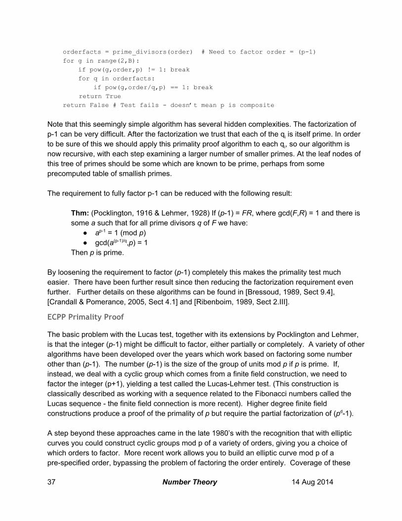
orderfacts = prime_divisors(order) # Need to factor order = (p­1) for g in range(2,B): if pow(g,order,p) != 1: break for q in orderfacts: if pow(g,order/q,p) == 1: break

return True return False # Test fails ­ doesn’t mean p is composite Note that this seemingly simple algorithm has several hidden complexities. The factorization of p­1 can be very difficult. After the factorization we trust that each of the qi is itself prime. In order to be sure of this we should apply this primality proof algorithm to each qi, so our algorithm is now recursive, with each step examining a larger number of smaller primes. At the leaf nodes of this tree of primes should be some which are known to be prime, perhaps from some precomputed table of smallish primes. The requirement to fully factor p­1 can be reduced with the following result:

Thm: (Pocklington, 1916 & Lehmer, 1928) If (p­1) = FR, where gcd(F,R) = 1 and there is some a such that for all prime divisors q of F we have:

ap­1 = 1 (mod p) gcd(a(p­1)/q,p) = 1

Then p is prime. By loosening the requirement to factor (p­1) completely this makes the primality test much easier. There have been further result since then reducing the factorization requirement even further. Further details on these algorithms can be found in [Bressoud, 1989, Sect 9.4], [Crandall & Pomerance, 2005, Sect 4.1] and [Ribenboim, 1989, Sect 2.III].

ECPP Primality Proof

The basic problem with the Lucas test, together with its extensions by Pocklington and Lehmer, is that the integer (p­1) might be difficult to factor, either partially or completely. A variety of other algorithms have been developed over the years which work based on factoring some number other than (p­1). The number (p­1) is the size of the group of units mod p if p is prime. If, instead, we deal with a cyclic group which comes from a finite field construction, we need to factor the integer (p+1), yielding a test called the Lucas­Lehmer test. (This construction is classically described as working with a sequence related to the Fibonacci numbers called the Lucas sequence ­ the finite field connection is more recent). Higher degree finite field constructions produce a proof of the primality of p but require the partial factorization of (pd­1). A step beyond these approaches came in the late 1980’s with the recognition that with elliptic curves you could construct cyclic groups mod p of a variety of orders, giving you a choice of which orders to factor. More recent work allows you to build an elliptic curve mod p of a pre­specified order, bypassing the problem of factoring the order entirely. Coverage of these

37 Number Theory 14 Aug 2014

algorithms at various levels of detail can be found in [Bressoud, 1989, Sect 14.3], [Crandall & Pomerance, 2005, Sect 7.6], [Yan, 2009, Sect 2.6] and a survey paper by Pomerance [https://www.math.dartmouth.edu/~carlp/lucasprime3.pdf].

Factoring

Pollard (p-1) Algorithm:

The first factoring algorithm beyond basic trial division is Pollard's p­1 algorithm [Pollard, 1974]. While this algorithm is by no means the best algorithm for integer factoring its principles have been used in a variety of other algorithms including elliptic curve factoring, one of the current best algorithms. Consider some prime factor p of N. If we could magically find an exponent e such that e divides (p­1) then for almost any base b we would have:

be = 1 (mod p) [Fermat's Little Thm] be­1 = 0 (mod p) so be­1 = kp (mod N) and gcd(be, N) = p (probably, unless k also divides N)

This, of course, avoids the question of how we found the magic exponent e. We will outline one popular approach. Guess a limit L such that L is greater than all prime factors of (p­1) (remember, you don’t know the value of p, so this is just a guess). Now let e = (L!). This gives us the following algorithm:

Algorithm: (Factoring Integer N) [Pollard p­1] b = 2 (for instance ­ other bases should work) for i=1 to L b = bi (mod N) (from b(i­1)! compute bi!)

if gcd(b­1, N) is not 1 print "a factor of ",N," is ",gcd(b­1,N)

Which can be implemented with the following simple Python routine. Here we use a simple heuristic bound of L = n1/8. Choosing an effective bound is an art form, balancing work versus likelihood of success. You probably don’t want to work too hard, as there are better practical ways to factor. def factorPm1(n): b = 2 # Choose a base ­ 2 is probably good enough # Choosing a bound is an art ­ balance work for success l = (1 << int(math.log(n)/8)) for (i in range(l)):

38 Number Theory 14 Aug 2014

b = pow(b,i,n) # Given b((i­1)!) compute b(i!) fact = gcd(b­1,n) if (fact != 1) and (fact != n): return fact Analysis:

Let p­1 have a prime power factorization of is p­1 = qiei.∏

qi prime ≤L

Then assume that qiei divides Q! for some integer Q.∏

qi prime ≤L

There are two leaps of faith here: 1. qL ≤ Q (need a large enough Q and the luck to have small qi) 2. ∀i ei ≤ ⌊Q/qi⌋ + ⌊Q/qi2⌋ + ⌊Q/qi3⌋ + ... (very likely to be satisfied, it turns out)

As the most important condition ends up being the first we will identify Q with L and satisfy ourselves with finding a value for L which is larger than every prime qi dividing p­1. Now we need to analyze the work factor and the probability of success of Pollard p­1. Here we view single modular multiply as a basic operation (a false assumption for very large numbers, but one which is easy to correct after the fact). The above implementation has a gcd every iteration. As the work of a gcd is O(log(N)) and there are L iterations, the work for the gcd computations is O(L log(N)). (A careful look at the algorithm shows that with some care one really only needs to run a single gcd at the last step, so this is not a major part of the work factor.) Each modular exponentiation, bi, has a cost of O(log(i)), so the total cost is ∑i≤Llog(i). Approximating this sum as an integral we get: ∑i≤Llog(i) = ∫i=1Llog(i) = (L log(L) ­ L + 1) = O(L log(L)). Before computing the probability of success for this algorithm we need to cite some advanced results from analytic number theory:

Defn: A number N is B­smooth if it has no prime divisors larger than some bound B. Examples: 135 = (5)(33) is 7­smooth and 5­smooth, but not 3­smooth or 2­smooth. 1234567890 = (2)(32)(5)(3607)(3803) is 5000­smooth and 3803­smooth, but not 3607­smooth or 5­smooth. Defn: ψ(N, L) is defined as the number of integers greater than zero and less than or equal to N which are L smooth. Examples: ψ(20,3) = 10 (1,2,3,4,6,8,9,12,16,18) and ψ(30,5) = 18 (1,2,3,4,5,6,8,9,10,12,15,16,18,20,24,25,27,30). Thm: (Dickman, 1930) ψ(N, L) ∼ N ρ(logN/logL), where ρ(u) is the Dickman function, with asymptotic behavior ρ(u) ∼ u­u

39 Number Theory 14 Aug 2014

Thus, if we ignore the effect of the size of the exponents ei (leap of faith ii) we can compute the probability of success as:

Prob = ψ(p­1, L)/p ∼ (logp/logL)­(logp/logL) More details on this algorithm and its analysis can be found in a number of sources, among them [Axler & Childs, 2009, Sect 10.C], [Bressoud, 1989, Sect 5.4], [Stein, 2009, Sect 6.3.1], [Yan, 2009, Algor 3.2.5], [Cohen, 1993, Sect 8.8] and [Crandall & Pomerance, 2005, Sect 5.4]. Although the p­1 algorithm is rarely used now as a general factoring algorithm, it is the inspiration for the elliptic curve factoring method, which is the state of the art.

Pollard Rho Algorithm:

We now come to Pollard’s Rho factoring algorithm [Pollard, 1975]. This factoring algorithm is very effective in practice, is easy to program and describe, but unfortunately relies on some ideas from the field of random mappings ­ far from number theory ­ in order to understand how effective it is.

Algorithm: (Factoring Integer N) [Pollard Rho] x ← 2 (a randomly chosen start point) y ← x while gcd(x­y, N) == 1 x ← x2 + 1 x ← x2 + 1 y ← y2 + 1 print "a factor of ",N," is ",gcd(x­y,N)

An implementation of this algorithm in Python: def factorPR(n): """factorPR(n) ­ Find a factor of n using the Pollard Rho method. Note: This method will occasionally fail.""" for slow in [2,3,4,6]: numsteps=2*math.floor(math.sqrt(math.sqrt(n))); fast=slow; i=1 while i<numsteps: slow = (slow*slow + 1) % n i = i + 1 fast = (fast*fast + 1) % n fast = (fast*fast + 1) % n g = gcd(fast­slow,n) if (g != 1): if (g == n): break else: return g # Return a non­trivial factor

40 Number Theory 14 Aug 2014

return 1 # Fail The effectiveness of the Pollard Rho algorithm, and its unusual name, come from the expected result when a random map f:S­­>S on a finite set S is applied to some initial element x0. If we define f(x0) = x1, f(x1)=x2, f(x2)=x3, etc, then eventually some xi will equal some earlier element xk. After that we will be forced to have xi+1 = f(xi) = f(xk) = xk+1 and xi+2=xk+2, etc, forming a loop or cycle of length (i­k). The initial sequence of elements x0,...,xk­1 are said to form the tail. With a little imagination the tail, together with the loop or cycle, can be seen to look like a letter p, or the greek letter rho (ρ).

Defn: Given a map β:S→S, a cycle of β is a set of elements in S, x0, x0, ... xn­1, such that for each i β:xi→xi+1 and β:xn­1→x0. The length of the cycle is n. Defn: If y is not on any cycle of β but l is the smallest integer such that βl(y) is on a cycle, then the elements y, β(y), ..., βl­1(y) is the tail of β starting at y and l is the length of the tail. Thm: (Sort of, once the definitions are tightened up, but close enough for our needs) For random maps β:S→S (where S is a finite set of cardinality N) the average cycle configuration consists of a single cycle of length √N. Most points in the set are on tails of average length √N emptying into this cycle.

With a little thought these results can be made plausible with simple probability arguments of the sort used to demonstrate the birthday paradox. The first algorithm using these principles is Pollard’s Rho factoring algorithm. This algorithm is named by the fact that a cycle with a tail looks like the greek letter ρ. We use this algorithm to factor a composite integer N. Let q be one of the factors, so N=qc. The idea is this ­ We use a random map which acts not just on ZN, but also on Zq. The most commonly chosen such map is β:x → x2+1. Now we expect that x will be on a tail and cycle of combined length about 2√q in Zq. We run two points on this cycle, one quickly, x, and one slowly, y. We expect that after about 2√q steps that x ≡ y (mod q). When this happens we have x­y will divide q and gcd(x­y, N) will be q. Thus we get a factoring algorithm with work factor O(√q) or (assuming the worst case, that q = √N) O(N1/4). A more careful analysis and more efficient variants can be found in [Axler & Childs, 2009, Sect 22.D], [Bressoud, 1989, Sect 5.3], [Cohen, 1993, Sect 8.5], [Crandall & Pomerance, 2005, Sect 5.2.1], [Sedgewick & Flajolet, 2013, Sect 9.8], [Yan, 2009, Algor 3.2.4] and [Knuth, v2, Sect 4.5.4, Algor B], among other places.

41 Number Theory 14 Aug 2014

Other Factoring Algorithms:

The current state of the art in factoring is dominated by the elliptic curve factoring method (ECM) and various sieving algorithms. In general it can be said that ECM is best when attempting to recover moderate sized factors, while sieving algorithms are best applied when the factors are all expected to be very large (in the limiting case commonly used by RSA there can be two factors, each of size about the square root of the composite number). The elliptic curve factoring method (ECM) is essentially a re­implementation of Pollard’s p­1 algorithm, but replacing operations (mod N) by operations in an elliptic curve group (mod N). Large parts of the analysis remain unchanged, with the major difference that, if the group order ((p­1) in the case of Pollard, o(EN) in the case of ECM) appears to have large factors, the user of ECM has the option of trying a new curve with possibly a better group order, while the user of Pollard is stuck with the one (p­1) he has been presented with. Coverages of ECM ranging from accessible to complete can be found in [Bressoud, 1989, Sect 14.2], [Stein, 2009, Sect 6.3], [Cohen, 1993, Sect 10.3], [Yan, 2009, Sect 3.3] and [Crandall & Pomerance, 2005, Sect 7.4]. Sieving factoring algorithms range from the time honored quadratic sieve to the current state of the art number field sieve. The detailed nature of these algorithms defy even outlining the algorithms in a paragraph or two. [Bressoud, 1989, Chap 8], [Cohen, 1993, Sect 10.4 & 10.5], [Crandall & Pomerance, 2005, Chap 6], [Yan, 2009, Sects 3.4­3.7] and [Knuth, v2, Sect 4.5.4, Algor B], among other places.

42 Number Theory 14 Aug 2014