7 D-AIl~SS 548 ABRIEF REVIEN OF ADAPTIVE NULL STEERING TECHNIGUES(U) 1/1I RL SIGNALS AND RADAR ESTAGLISHNENT NALVERN (ENGLAND)I J G MCNNIRTER FEB 86 RSRE-MIEMO-3939 DRIC-OR-99244

UNCLASSIFIED F/G 26/4 N

13,15

13."

I IIIIN 10 2 8li

___=__ 14 lU15

f1*2 5 1*_ 4 _

V -..

S.

UNLIMITED .;

00

... RSRE

* MEMORANDUM No. 3939

ROYAL SIGNALS & RADARESTABLISHMENT

A BRIEF REVIEW OF ADAPTIVE NULLSTEERING TECHNIQUES

Author: J G McWhirter

d PROCUREMENT EXECUTIVE,

z MINISTRY OF DEFENCE,

RSRE MALVERN;

o WORCS. T-)Icz LC

~JUL 1 9 U14,11

U)

UNLIMITED 06 J,

ROYAL SIGNALS AND RADAR ESTABLISHMENT

Memorandum 3939

Title: A BRIEF REVIEW OF ADAPTIVE NULL STEERING TECHNIQUES

Author: J G McWhirter

Date: February 1986

SUMMARY

.!A brief theoretical review of adaptive null steering is presented. The

basic theory is first outlined in the context of sidelobe cancellationsystems as well as general antenna arrays. Various approaches to the

practical implementation of adaptive null steering are then discussed.These fall ito the two main categories of closed loop methods and directsolution m~gods. The closed loop methods are very cost-effective andsuitable in principle, for either analogue or digitial processing. Howevertheir rate of convergence is fundamentally limited and too slow for someapplications. The direct solution methods do not suffer from this problembut tend to be suitable only for digital processing and are more expensive

from the computational point of view. However they are well suited toparallel processing and now provide a very practical alternative due torecent advances in VLSI circuit technology. A brief discussion on the

effects of multi-path propaatiQn on adaptive null steering systemsconcludes this 1-i-itr)reviewt. .-

r 7

- ... '0...) :: it; C des 0'"

Copyright -.

CController HMSO London

1986

58.0/59

W-9' FT. A- I.-W -r ra

A BRIEF REVIEW OF ADAPTIVE NULL STEERING TECHNIQUES

J G McWhirter

PREFACEp .4

This brief review was prepared originally as one section of a TTCP reporton "Antenna Array Signal Processing" produced by a study group from the

KTP3 panel. It only provides a theoretical discussion of the key signalprocessing techniques and how they are perceived to be evolving. It does

not address any of the wider system or technology related issues and wasnever intended as a comprehensive review of the entire subject. It hasbeen produced here as a stand alone document in response to a request from .

several readers who felt that it provides a good introduction to thesubject and should be more readily available. I am grateful to them for

their comments and hope that this memorandum may indeed prove to be useful 6

in that context.

...

.,£.,

"'S

A BRIEF REVIEW OF ADAPTIVE NULL STEERING TECHNIQUES

J G McWhirter

CONTENTS

1 INTRODUCTION

2 BASIC THEORY

2.1 Sidelobe Cancellation

2.2 General Arrays

3 IMPLEMENTATION '-

3.1 Closed Loop Methods

3.1.1 Howells-Applebaum

3.1.2 Widrow LMS Algorithms

3.1.3 Hybrid Analogue/Digital Techniques

3.2 Direct Solution Methods

3.2.1 Sample Matrix Inversion

3.2.2 Gram-Schmidt

3.2.3 Sequential Decorrelation

3.2.4 QR Decomposition

3.2.5 The Hung and Turner Algorithm

4 EFFECTS OF MULTIPATH

4.1 Jammer Multipath I

4.2 Signal Multipath

5 REFERENCES

U'-a.

d;

i i

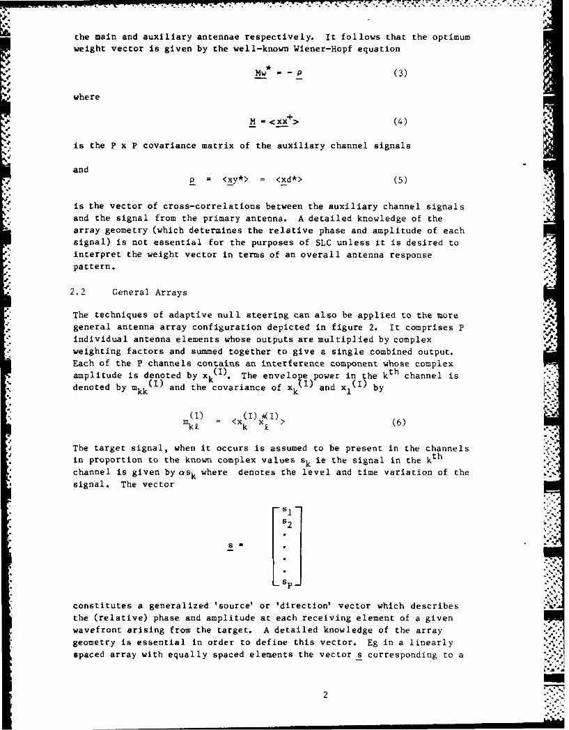
INTRODUCTION

The ability to control the phase and amplitude of the received signal in

each channel of an antenna array makes it possible to implement various

types of adaptive signal processing. In adaptive antenna array signalprocessing the vector of complex weights w and hence the shape of the

received beam is determined as a function of the received signal data and

can change in response to the signal environment. The most common

application of adaptive beamforming is adaptive null steering which

constitutes a powerful technique for the suppression of jammer signals in a

radar or communications systems.

2 BASIC THEORY

In this section the problem of adaptive null steering will be considered in

its most general form without reference to specific implementation or

application.

2.1 Sidelobe Cancellation

The technique of adaptive null steering was pioneered in the early 1960's

by P Howells (then with General Electric in Syracuse) and S Applebaum

(Syracuse University Research Corporation) in the context of (coherent)

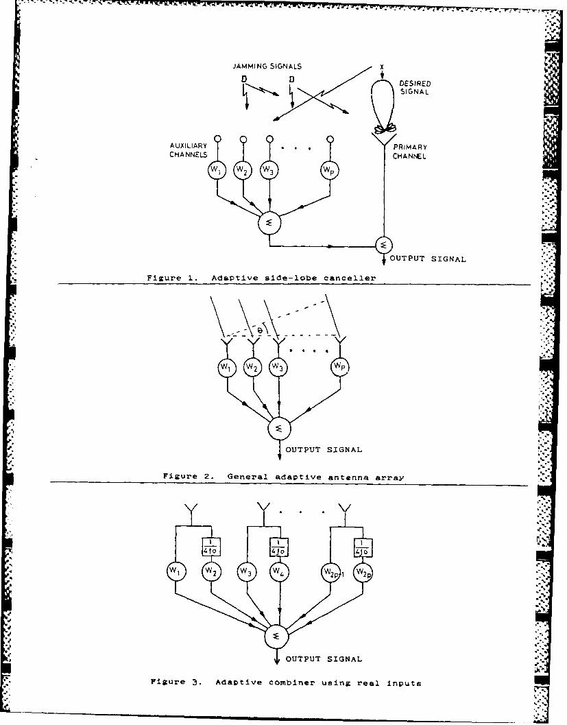
side-lobe cancellation (SLC) [ I ] . A typical sidelobe cancellation system isdepicted in figure 1. It consists of a main, high gain antenna whose

output is designated as channel P+l and P auxiliary antennae. The

auxiliary antenna gains are designed to approximate the average sidelobe

level of the main antenna gain pattern. The amount of desired target

signal received by the auxiliaries is assumed to be negligible compared to

the target signal d in the main channel. The purpose of the auxiliaries isto provide independent replicas of jamming signals in the sidelobes of the

main pattern for cancellation. The auxiliary outputs are weighted and

summed and the combined signal is added to the signal in the primary

channel. The problem is to find a suitable means of controlling the weight

w so that the maximum possible cancellation is achieved.

In the case of SLC it can easily be shown that the maximum output SNR is

obtained when the total output power is minimized provided that the target*. signal d in the main antenna is not correlated with any of the auxiliary

signals. The weight vector w must therefore be chosen to minimize the

quantity

E = <!e! 2 > I)

where

e= y + xTw 2

and y and x1 (i 1,2 ...P) denote the complex amplitudes of the signals in

* - . .

the main and auxiliary antennae respectively. It follows that the optimum

weight vector is given by the well-known Wiener-Hopf equation

Mw P (3)

where

M - <xx+> (4)

is the P x P covariance matrix of the auxiliary channel signals

andp = <xy*> = <xd*> (5)

is the vector of cross-correlations between the auxiliary channel signals

and the signal from the primary antenna. A detailed knowledge of the

array geometry (which determines the relative phase and amplitude of each

signal) is not essential for the purposes of SLC unless it is desired tointerpret the weight vector in terms of an overall antenna response

pattern.

2.2 General Arrays

The techniques of adaptive null steering can also be applied to the moregeneral antenna array configuration depicted in figure 2. It comprises P.9'

" individual antenna elements whose outputs are multiplied by complexweighting factors and summed together to give a single combined output.

Each of the P channels contains an interference component whose complex

amplitude is denoted by xk(I). The envelope power in the kth channel isdnt by (I) hn Mdenoted by mkk and the covariance of xk and x I by

(I)(I) *(i)(6=m X <x (6)

The target signal, when it occurs is assumed to be present in the channelsin proportion to the known complex values sk ie the signal in the kth

channel is given by ask where denotes the level and time variation of thesignal. The vector

-S

*L spi

constitutes a generalized 'source' or 'direction' vector which describesthe (relative) phase and amplitude at each receiving element of a givenwavefront arising from the target. A detailed knowledge of the arraygeometry is essential in order to define this vector. Eg in a linearly•

spaced array with equally spaced elements the vector s corresponding to a V

2....'

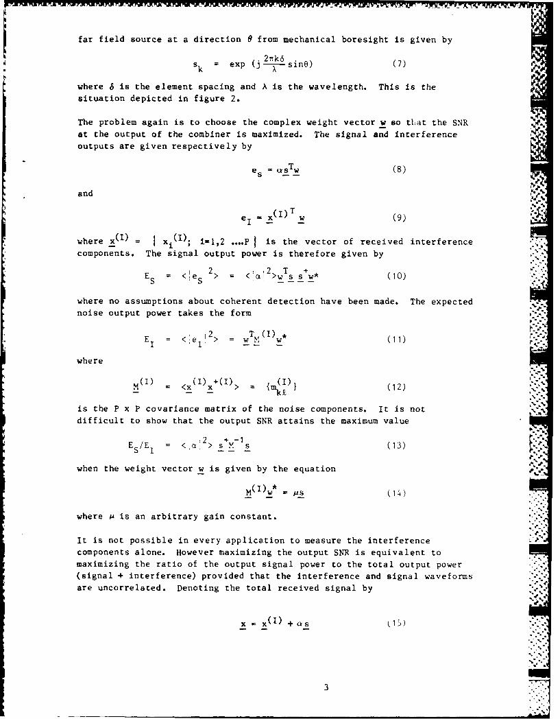
far field source at a direction 8 from mechanical boresight is given by

sk = exp (j- sine) (7)

where 6 is the element spacing and A is the wavelength. This is the

situation depicted in figure 2.

The problem again is to choose the complex weight vector w so tiat the SNR

at the output of the combiner is maximized. The signal and interference

outputs are given respectively by

es = QsTw (8)

and , X

eI = x()T (9)

wherex() = xi(I); i=1,2 .... P is the vector of received interference

components. The signal output power is therefore given by ..

12e> = <jaQ2>wTs s w*

where no assumptions about coherent detection have been made. The expected

noise output power takes the form -

E = <'e > = wM(w (11)

where

M = <x ) x+ > mkZ (12)

is the P x P covariance matrix of the noise components. It is not %difficult to show that the output SNR attains the maximum value

E/E = <,2 >sM (13)SE " -

when the weight vector w is given by the equation

M(I)w* =As (14)

where P is an arbitrary gain constant.

It is not possible in every application to measure the interference

components alone. However maximizing the output SNR is equivalent to

maximizing the ratio of the output signal power to the total output power

(signal + interference) provided that the interference and signal waveforms

are uncorrelated. Denoting the total received signal by

x (I) s (15)

3

T -- 77 -7- V - Y Y -3

the total output power is given by

E <e +ei!2> = w TMW* (16)

whereM = < x x+>

= M + <c 2 > ss+ (17)

ie the P x P covariance matrix of the output signal plus noise from the P

channels. The ratio Es/Es+I is maximized when the weight vector satisfiesthe equation

Mw = (18)

It can easily be vhown that the solution to equation (18) must also

satisfy equation (14) and so the two are analytically equivalent.

However they have different numerical properties which must be taken into

account when considering any practical implementation. The more generalsolution in equation (18) will be assumed in the remainder of this

report.

Determining the optimum weight vector w for a general adaptive antenna .array can also be formulated as a constrained minimization problem definedas follows. Find the weight vector w which minimizes the total output

power as defined in equation (1) but with

e =xTw (19)

• .subject to the constraint that

TS w = (20)

This constraint ensures that the antenna gain in the target 'look-

direction' is held at a constant value, and hence the signal power in

equation (8) is maintained during adaptation. The constrainedminimization problem defined above can be solved quite readily using the

conventional method of Lagrange undetermined multipliers. The solution is

given by 4

Mw* =s/(s + M- s) (21)1

which is clearly equivalent to that given in equation (18), the

arbitrary gain constant u being chosen to ensure that the constraint in

equation (20) is satisfied.

4.'..:::

40

% N 7 .....

It is interesting to note that the results derived for adaptive SLC may bederived as a special case of the more general antenna array results above.Since the target signal in SLC is present only in the p+Ith channel the 0Pappropriate source vector is X.

J = [0,0,0 .......... 0,1] (22) .S..

and the optimum P+1 element weight vector w' must satisfy

M'W' - ;At (23)

where M' is the (P+I) x (P+I) covariance matrix of all the channels.

Equation (23) may be partitioned in the form

(24)

where Ep+l is the power output of the main channel and M and p are defined inequations (4) and (3). It follows that the weight vector for the

auxiliary channels must satisfy

Mw* (25)

which is equivalent to the result in equation (3) since the parameter• and hence the weight wp+ may be chosen arbitrarily.

V l

So far in this section it has been assumed that all signal and noise

components are narrowband and a single complex quantity has been used todescribe the output from each channel. However, each complex signal *..

sample may be replaced by two real samples as illustrated in figure 3. Thesample time for the second of these is delayed relative to the first by1/4f where f is the appropriate cen tre frequency and a separate real weightfactor w is applied to each one. Alternatively the baseband

land Q signals may be treated as two independent real signals. This approach Nas

significant advantages for adaptive nulling since the algorithmis released fromunnecessary constraints imposed by the

complex signal representation and becomes less sensitive toproblems of I and Q imbalance. The theory outlined above is clearly

applicable to the 2P real signals which must be combined in this situation.

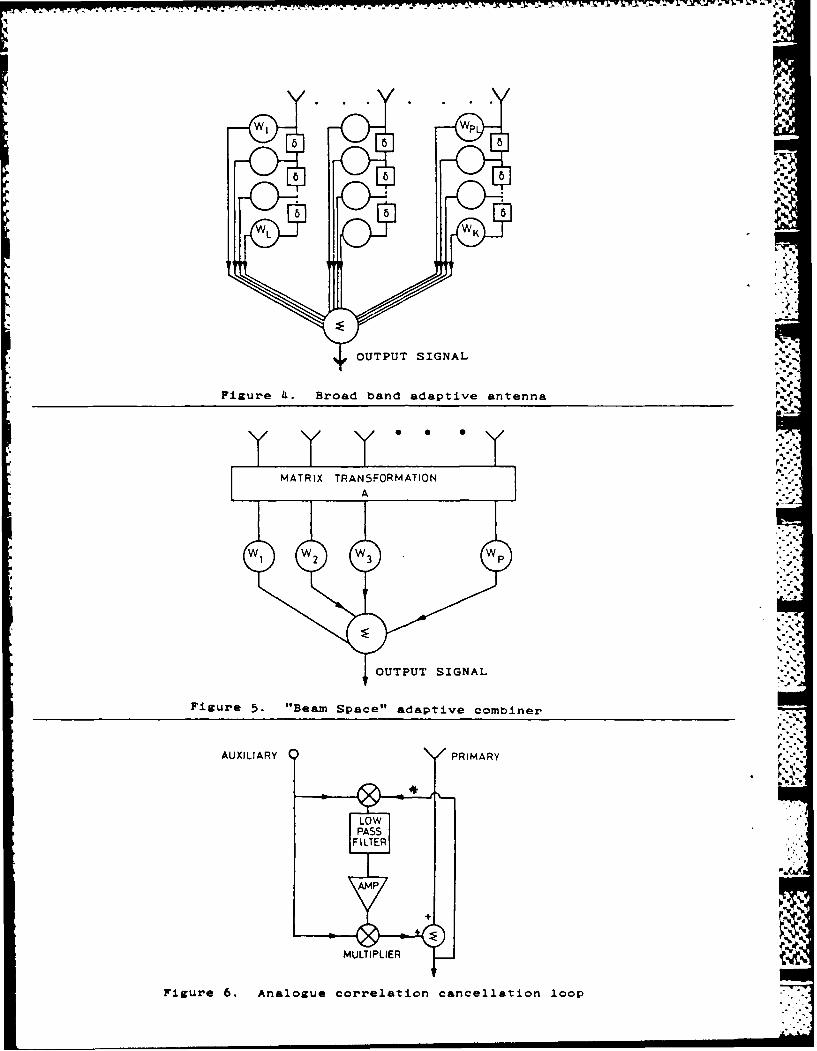
It can also be applied to situations in which the received signals arebroadband.[ 3) The signals may then be represented by means of a sequence

of delayed sample values which could be stored in tapped delay lines as

illustrated in figure 4. For a signal bandwidth B, the appropriate delayinterval is 1/4B and the number of delays is given by B/fres where fres isthe required frequency resolution. Each sample in every receiver channelis multiplied by an individual (real) weighting factor wi and the resulting

products are suumed together to form the combined output. For the purpose

of applying the theory outlined above, the PL samples (assuming P antenna

elements and L samples in each delay lines) are simply treated as elements

5

-0* Y-..- -. - A X.w

of a single sample vector x and the output of the combiner may again be

enxtesse ofn the r TX where w is the corresponding PLxI weight vector.In he aseof LC heoutput of the combiner is added to the signal

received by the primary antenna and the weights are adjusted to ensure that

the output power is minimized. In the general antenna array case theweights are adjusted to minimize the output power of the combiner itselfsubject to L constraints of the form

T =i 1,2 ....... L (26)

which can be used to ensure that the desired frequency response in a givenlook direction is maintained. 14

Most of the methods described in this section can be applied either in* element space or in beam space although the former will be assumed in this*report. Element space refers to the situation outlined in figure 2 where

the adaptive nulling is performed by linearly combining the signals which* emerge from the antenna elements. Beam space refers to the situation in

*which a preliminary fixed linear combination of the signals is performed toproduce P beams with some desired characteristics as illustrated in figure

5. Since a linear combination of the beams also constitutes a linearcombination of the received signals, adaptive nulling in beam space shouldyield the same overall antenna response as adaptive nulling in elementspace even though a different weight vector is computed. The same theorycan be applied in each situation and no distinction will therefore be drawn

* between the two types of application.

3 IMPLEMENTATiON

* In this section we will review the main techniques which have been devised* for implementing adaptive null steering including some very recent

developments. The methods may be divided into two main categories. Theseare (1) Closed loop or feedback control techniques and (2) Direct solutionmethods (often referred to as 'open-loop'). Broadly speaking closed loopmethods are cheaper and simpler to implement than direct solution methods.

*By virtue of their self correcting nature, they do not require components* which have a wide dynamic or high degree of linearity and so they are well

suited to analogue implementation. However closed loop methods suffer fromthe fundamental limitation that their speed of response must be restrictedin order to achieve stable operation. Direct solution methods on the other

* hand do not suffer from problems of slow convergence but in general theyrequire components of such high accuracy and wide dynamic range that they

can only be realised by digital means. of course closed loop methods canalso be implemented using digital circuitry, in which case the constraints

* on numerical accuracy are greatly relaxed and the total number of* arithmetic operations is much reduced by comparison with direct solution

methods.*

67

3.1 Closed Loop Methods

In this subsection we will briefly review the main closed loop methods bothanalogue and digital. These methods are now well established and were

discussed in a previous report. rb.'

3.1.1 Howells-Applebaum

Much of the pioneering work on adaptive antenna arrays was carried out by

Howells and Applebaum in the 19601s.[l] The analogue correlation loop

which they developed is illustrated schematically in figure 6 for a simple

two channel configuration. The auxiliary signal x is multiplied by a

complex weight factor w and added to the signal in the primary channel y.

The weight is derived by correlating x with the residual signal e. The

correlation process is either carried out at RF using suitable mixers or at

IF using an analogue multiplier and lowpass filter (or integrator). When

it has converged to a steady state the output of the loop is uncorrelated

with the signal x provided that the gain of the amplifier is sufficiently

high. This type of canceller has developed considerably over the last two

decades and is now capable of achieving a level of performance in the

laboratory comfortably in excess of that likely to be required in the

field. A fairly cheap version implemented as a thin film hybrid circuit

has been produced by the Hughes Aircraft Company.[2]

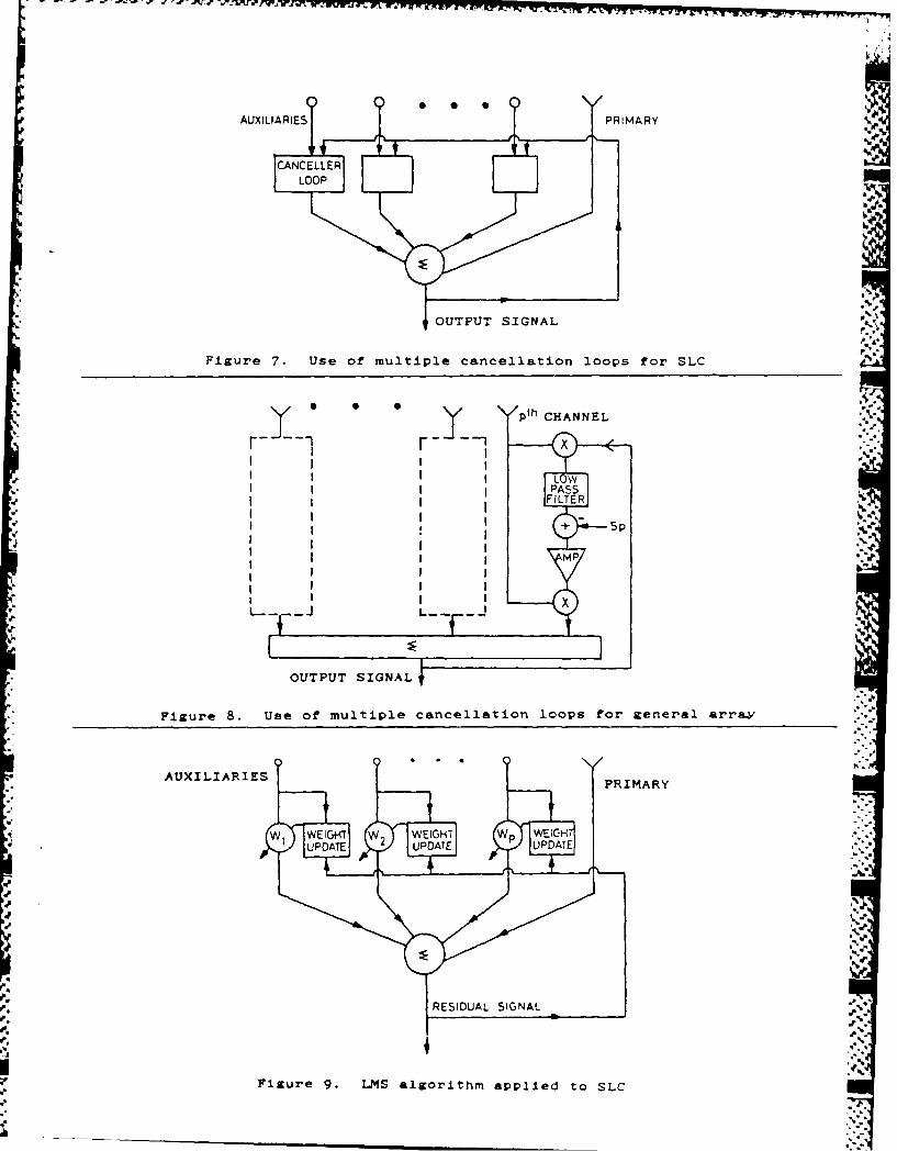
Figure 7 shows schematically how a number of correlation cancellation loops

may be used in parallel to implement a multiple sidelobe cancellation

system. When each correlation loop has converged to a steady state the

residual signal e is uncorrelated with each of the auxiliary signals xk

and so the energy of the residual signal is minimized. It is not difficult

to show that the weight vector is then given by the expression

(M + Ip/G)w =-P (27)p - -

where I is the PxP identity matrix and M and P are as defined previously.-p

This is equivalent to the Wiener-Hopf solution given in equation (3)

provided that the amplifier gain G is large.

Figure 8 illustrates the use of several parallel correlation cancellationloops to perform adaptive nulling in the case of a general antenna array

for which the desired look direction is specified by the vector s. The

weights wk are derived by correlating each signal xk with the output signal

e, adding the correlation output to the desired vector component sk and

then using a high gain amplifier. In this case the steady state weight

vector is given by the equation

(M + I /G)w = s (..p-.

which clearly takes the same form as the optimum control law given in

equation (18) provided, once again, that the a:p-if iur gain GA i-

sufficiently large.

7]

|

3.1.2 Widrow LMS Algorithm

The Least Mean Square (LMS) algorithm developed by Widrow is an entirel

digital, closed loop control algorithm suitable for adaptive nulling.[3T

Figure 9 illustrates the use of this algorithm for multiple sidelobe ON

cancellation. The P signals xk(n) are multiplied by complex weighting

coefficients wk and summed together to produce the secondary signal a(n)which, in turn, is added to the primary signal y(n) to produce the output

residual signal

e(n) = xT(n)w + y(n) (29)

The vector of weights w is updated according to the formula

w(n+l) = w(n) + 2e* (n)x(n) (30)

where x(n) denotes the vector of signal samples which enter the combiner at

the ntt discrete time sample and u is a constant gain factor. Thealgorithm is particularly efficient, requiring only -4P real

multiplications and -4P real additions per sample time to update the weight

vector. The update formula for each coefficient wk is clearly of the form

wk(n+l) wk(n) + 2Ae (n)xk(n) (31)

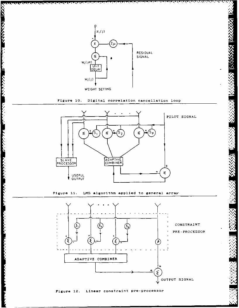
which defines a simple digital correlation cancellation loop of the typeillustrated in figure 10. The LMS algorithm, in effect, constitutes Psuch loops operating in parallel with a common gain factor and is the

digital equivalent of the Howells-Applebaum technique discussed above.

Widrow has shown that if the weight vector is updated according to equation(30) then

<w*(n)> - -M P (32)-n-+o -,

(ie the weight vector tends in the mean to the optimum value given in

* equation (3) provided that the gain constant M satisfies the

condition

0 < < 1 (33)max

where Nmax denotes the largest eigenvalue of the covariance matrix M.

Footnote: For simplicity it has been assumed that one complexmultiplication is equivalent to 4 real multiplications and 2 real

additions.

8*1 q

N'".

The rate of convergence depends on the value of A. For small values of

P the algorithm converges slowly and the weight vector does not fluctuate

too much about the mean. For large values of p the algorithm converges

more rapidly but the weight vector is subject to larger fluctuations due to

the fact that the integration time of the loop and hence the statistical

accuracy is reduced. These fluctuations in turn lead to 'misadjustment

noise' which causes the output energy to increase above its optimum level. a.J.

The time constant of adaption for the k th normal component of the weight

vector (ie the component associated with the kth eigenvector of M) is

given by

T = (34)

k 2a.. A

where is thhwhere Xk is the k

h eigenvalue and so, if the spread of eigenvalues is

large, the smaller components must suffer very slow convergence if the

stability condition (33) is to be satisfied. -This fundamental limit

to the overall rate of convergence is common to all of the closed loop

techniques for adaptive nulling.

In the above discussion it has been assumed for consistency that the P

signals xk(n) which enter the combiner are complex. However it is worth

pointing out that the LMS algorithm may also be applied to the 2P real

signal components from a P-element narrow-band array of the type depicted .

in figure 3 or the PL real signals from a broadband receiver array of the

type illustrated in figure 4 .3]-

So far the Widrow LMS algorithm has been discussed only in the context of

adaptive sidelobe cancellation. It can also be applied to the problem of

adaptive nulling for a general antenna array but most of the methods which

have been proposed for incorporating the look direction constraint vector

are rather cumbersome. Widrow suggested the use of a pilot signal to

emulate the effect of the primary signal in a sidelobe canceller.[3 ] The , a*

scheme which he proposed is shown in figure 1i. The pilot signal d is fed

into each receiver channel with the relative phase and amplitude factors .

appropriate to a signal received by the antenna array from the required

look direction, ie the signal vector ds is input to the array. The LMS

algorithm is then used to minimise the sum of the array output and the

desired signal. As a result the array is constrained to have a strong

response in the required look direction whilst nulling out other

uncorrelated signals. The resulting weight vector must also be applied to

the received signals in the abscence of the pilot signal (using an

additional 'slave processor') in order to determine the time output of the

array. This technique is expensive to implement and has been shown to lead

in general to a biassed solution. .:

9 . °1.

: -: .:.

Griffiths [5 ] has suggested a different technique for applying the Widrow

LMS algorithm to adaptive nulling with a general array. He assumes that

* the cross-correlation vector between the desired signal d(n) and the vector

of received signals x(n) is known. The update equation (30) for the

weight vector is expressed in the form

w(n+l) = w(n) + 2M(y*(n) + o*(n))x(n) (35)

and the quantity y*(n)x(n) is replaced by its mean value

p = <y*(n)x(n)> = <d*(n)x(n)> (36)

to provide the alternative update formula

w(n+1) = w(n) + 2/.(P + a * (n)x(n)) (37)

This equation involves a mixture of average and simultaneous quantities

but, as with the conventional LMS algorithm the weight vector w(n)

converges in the mean to the optimum value given in equation (3). The

weight vector update in this case requires-6P real multiplications and-6P-.

real additions per sample time.

If the update formula in equation (37) is modified to take the form* t

w(n+l) = w(n) + 2p(-s + a (n)x(n)) (38)

where s is an appropriate look-direction constraint vector then the weight

vector should again converge in the mean according to equation (37)

but with P replaced by -s ie

<w*(n)> M-Is (39)- ~n-m .,

This is of course the optimum control law of equation (18). In effect

equation (38) is the digital equivalent of the technique proposed by

Applebaum for applying a directional constraint with analogue closed loops

as illustrated in figure 8. It does not require any knowledge about the

form of the desired signal d(n) - only its direction of arrival.

Frost proposed another method for applying the Widrow LMS algorithm to

adaptive nulling with a general array. He included the look-direction -

constraint (20) by introducing a Lagrange undetermined multiplier into

the gradient descent algorithm. The modified algorithm takes the form

w(n+l) = F[w(n) + 2Me*(n)x(n)] + f (40)

with W(o) = f

where f is a P-element vector given by

f = s(sTs)-6 (41)

10

"..X1W 1TMP 1WVW Z .r . 1- - - - . V: W -.

and F is the PxP projection matrix given by

F - - Ts)-Is1T (42)

The update formula (40) is clearly much more complicated to implement

than the basic LMS algorithm and requires an additional 8P real

multiplications and 10P real additions per sample time. However it does

operate in such a way as to ensure that the constraint equation (20)

is always satisfied exactly. This is not the case with the techniques

which Widrow and Griffiths proposed.

Frost's method was originally suggested for use with L simultaneous linear

constraints in a broadband application.1 4' However we have chosen todescribe it here for a single constraint in order to facilitate comparison

with the previous techniques. In the more general formulations the

constraint vector s becomes a PLxL constraint matrix and the scalar

6 becomes an L-element vector but the formula is otherwise identical.

A much simpler technique for incorporating the constraint equation(20) exactly has recently been proposed by McWhirter.[6 ] It was

originally developed for use with a direct solution algorithm based on themethod of QR decomposition which is discussed in section 3.2.4.

However it is worth describing at this stage since the technique is equally

applicable to the Widrow LMS algorithm. The technique can be explained

quite simply as follows. The constraint in equation (20) may be

written in the form

w = -s W (43)P

where ̂ s and w denote the first P-i elements of the vectors s and wrespectively and it has been assumed without loss of generality that

Sp M 1. By substituting this expression for wp into equation (19) itis possible to express the residual signal e in the form

e ZT + 6 x (44)

where

z xx (45)2

<lel 2 >must then be minimized with respect to the unconstrained P-i elementweight vector w. Equation (44) clearly takes the same form as .

equation (2) which describes the side-lobe cancellation problem. The

term Oxp plays the role of the primary signal y while the transformedvector Z corresponds to the auxiliary signal vector x. The general array

* problem with a single linear constraint has been transformed quite simply "

into an equivalent "end-element-clamped" configuration identical to that

for SLC. The "end-element-clamped" configuration may therefore be

considered as the canonical form for adaptive null steering and it is

assumed in the remainder of this report that any technique which is

suitable for SLC is equally applicable to the general array problem byapplying this transformation technique.

4..

21-

I I i

r-P p v pxTbrF.4u r u -O -. WWW~rWWW7113rV -7 XF 17M

The transformation may be applied using the type of pre-processor which isillustrated in Figure 12. It is implemented using only-4P real multiples

and -4p real additions. In effect the pth element (all elements areassumed to be equivalent in the general array problem) is arbitrary chosenas the primary channel which will in general receive signals from therequired look direction. The signal in this channel is then subtractedfrom the signal in each of the other channels using an appropriate phaseand amplitude weighting which ensures that the resultant signal has a nullin the required look direction. Consequently, adaptive combination of theresultant "auxiliary" signals cannot cancel any look direction signal in

the primary channel.

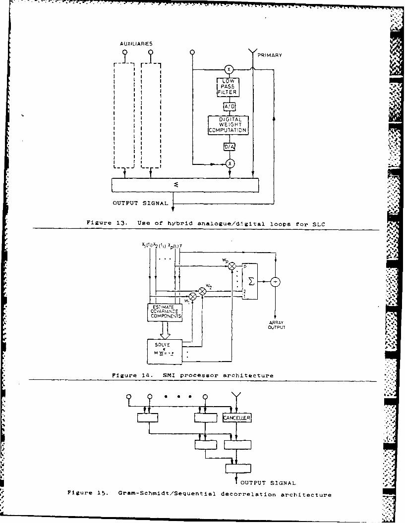
3.1.3 Hybrid Analogue/Digital Techniques

So far in this section we have described closed loop processing methodswhich are either entirely analogue or entirely digital. However a numberof hybrid analogue/digital methods have also been proposed in which theweight computation is carried out digitally but the weighting itself isperformed by analogue means. This combines the wide bandwidth and signalhandling capability of analogue circuits with the flexibility and high ,tdynamic range of digital circuitry. Figure 13 illustrates schematically anadaptive sidelobe canceller based on a hybrid loop which has been producedby the Hughes Aircraft Company.[7] In this case the multiplication of the .4.

residual signal by each of the auxilliary signals is also carried out usingan analogue multiplier and the product is passed through a losw-pass filterbefore being digitized. The weight vector can then be computed in a d

flexible way using, for example, techniques such as Powell's conjugategradient method for accelerated convergence. If the low pass filter wereomitted, the weight vector could be computed using the LMS algorithm given N,in equation (30) or even Frost's constrained LMS algorithm given inequation (40) (assuming a general array with no main beam signal).The hybrid approach in general allows the weights to be applied at a much

higher frequency than they are computed, the A/D conversion being carried 5

out at less than the Nyquist sample rate of the signals. This importantadvantage of the hybrid analogue/digital approach is not just relevant toclosed loop techniques but also to the direct solution methods which arediscussed in the next section. In any situation where the weights are

derived explicitly it should be assumed that they may be applied by eitheranalogue or digital means and so the use of hybrid analogue/digitaltechniques will not be discussed further in this chapter. Ir

3.2 Director Solution Methods

Very fast adaptive nulling is considered to be essential in a number of S.."

important military applications. For example the antenna array may be -mounted on a high speed rotating platform, it may have to cope with rapidlyswitched jammers or it may be required to change frequency rapidly for thepurposes of spread spectrum communications. In such situations directsolution methods are essential and a number of these will pow be discussed.

12

, V-°

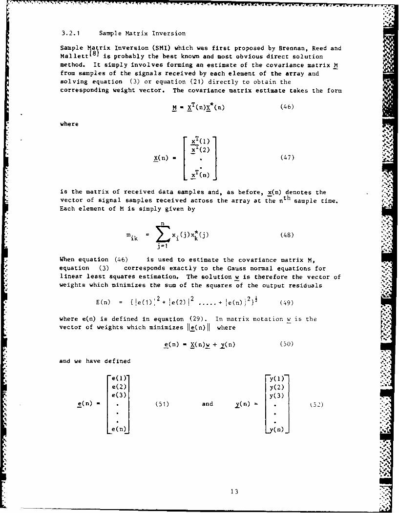
3.2.1 Sample Matrix Inversion

Sample Matrix Inversion (SMI) which was first proposed by Brennan, Reed andMallett [81 is probably the best known and most obvious direct solutionmethod. It simply involves forming an estimate of the covariance matrix Mfrom samples of the signals received by each element of the array and

solving equation (3) or equation (21) directly to obtain thecorresponding weight vector. The covariance matrix estimate takes the form

M -XT(n)X* (n) (46)

where

xTo)_T(2)

X(n) = (47)

LxT(n) j

is the matrix of received data samples and, as before, x(n) denotes thevector of signal samples received across the array at the nth sample time.

Each element of M is simply given by s

nm x (j)x*(j) (48)mik E xi (x k

1=1 1

When equation (46) is used to estimate the covariance matrix M,

equation (3) corresponds exactly to the Gauss normal equations forlinear least squares estimation. The solution w is therefore the vector ofweights which minimizes the sum of the squares of the output residuals

E(n) : {le( ) 12 + , e(2) 12 ...... + e(n) 12)1 (49)

where e(n) is defined in equation (29). In matrix notation w is the* vector of weights which minimizes Ile(n)I where

e(n) = X(n)w + Y(n) (50)

*. and we have defined

e(1)- y(1)-e(2) y(2)e(3) y(3)

e(n) = . (51) and .(n) • 2)

Le (n)j L(n)_

13

Similarly, equation (21) defines the optimum least squares solution to

the problem of minimizing IV£(n) H where

e(n) - X(n)W (53)

subject to the constraint in equation (20).

The SMI technique requires-2nP2 real multiplications and -2nP 2 real

additions in order to form the covariance matrix. In addition, -4P3/3 real

multiplications and-4p 3/3 real additions are required to compute the

weight vector solution (by Gaussian elimination). It should be noted that

when n>>P,computation of the covariance matrix is the dominant task,

requiring -2P real multiplications and-2P2 real additions per sample

time. Brennan, Reed and Mallett showed that for a P-element array only -2P

data vectors are required when forming the sample covariance matrix in

order to achieve an improvement in the output signal to noise power ratio

which is within 3 dB of the optimum statistical value. The rate of

adaptation is much faster therefore than that of a closed loop algorithm.

It is governed only by the statistical accuracy required and not by factors

such as stability and convergence time.

It is worth pointing our at this stage that "soft constraints" can also be

incorporated within the SMI technique. A soft constraint corresponding to

equation (20) is introduced by treating the constraint vector s as

though it were another data snapshot and appending it to the data matrix

X(n). The constant 0 is treated as the corresponding value for the signal

in the primary channel. Several constraints may be incorporated in this

way if required. Such constraints are not satisfied exactly, the

importance of each one being comparable only to that of a single data

snapshot within the overall least squares minimization. The influence of

any soft constraint may of course be enhanced by multiplying the

corresponding equation by a suitable scaling factor. As the scaling factor

is increased, the influcence of a soft constraint approaches that of the

equivalent hard constraint. However this technique is not recommended for

handling hard constraints since it must inevitably lead to a more ill-

conditioned matrix and so increase the dynamic range requirements of the

processor.

Soft constraints may be introduced in this way to any of the directsolution algorithms discussed in section 3.2. The same comments and

conclusions apply and so the subject will not be discussed further in this

report.

The sample matrix inversion technique leads quite naturally to a processor

architecture of the type illustrated schematically in figure 14 (for SLC).

It is quite conventional and comprises a number of distinct components -

one to form and store the covariance matrix estimate, one to compute the

solut'on of equation (3) and one to apply the resulting weight vector

to the auxiliary signal data. This data must be stored in a suitable

memory while the weight vector is being computed. The system also requires

a number of high speed data comnunication buses and a sophisticated control

unit to deliver the appropriate sequence of instructions to each component.

14

To -il 7Y -A %A -W 'P~~d7U ' a- . - V-V - *. -. f

This type of architecture is obviously complicated, extremely difficult todesign and not very suitable for VLSI.

Not only does the direct solution of equation (3) lead to acomplicated circuit architecture, it is also very poor from the numerical

point of view. The problem of solving a system of linear equations like

those defined in equation (3) can be ill-conditioned and hence

numerically unstable. The degree to which a system of linear equations is

ill-conditioned is determined by the condition number of the coefficientmatrix. The condition number of a matrix X is defined by

CCX) =() ~ ~

where X, and X are the largest and smallest (non-zero) singular values

respectively.[ The larger C(X) the more ill-conditioned is the system of

equations. It follows from equation (46) that

C(M(n)) = C(XT(n) X* (n)) = C2 (X(n)) (55)

and so the condition number of the estimated covariance matrix M(n) is muchgreater than than of the corresponding data matrix X(n). Any numerical

algorithm which avoids forming the estimated covariance matrix explicitlyand operates directly on the data is likely to be much better conditioned.

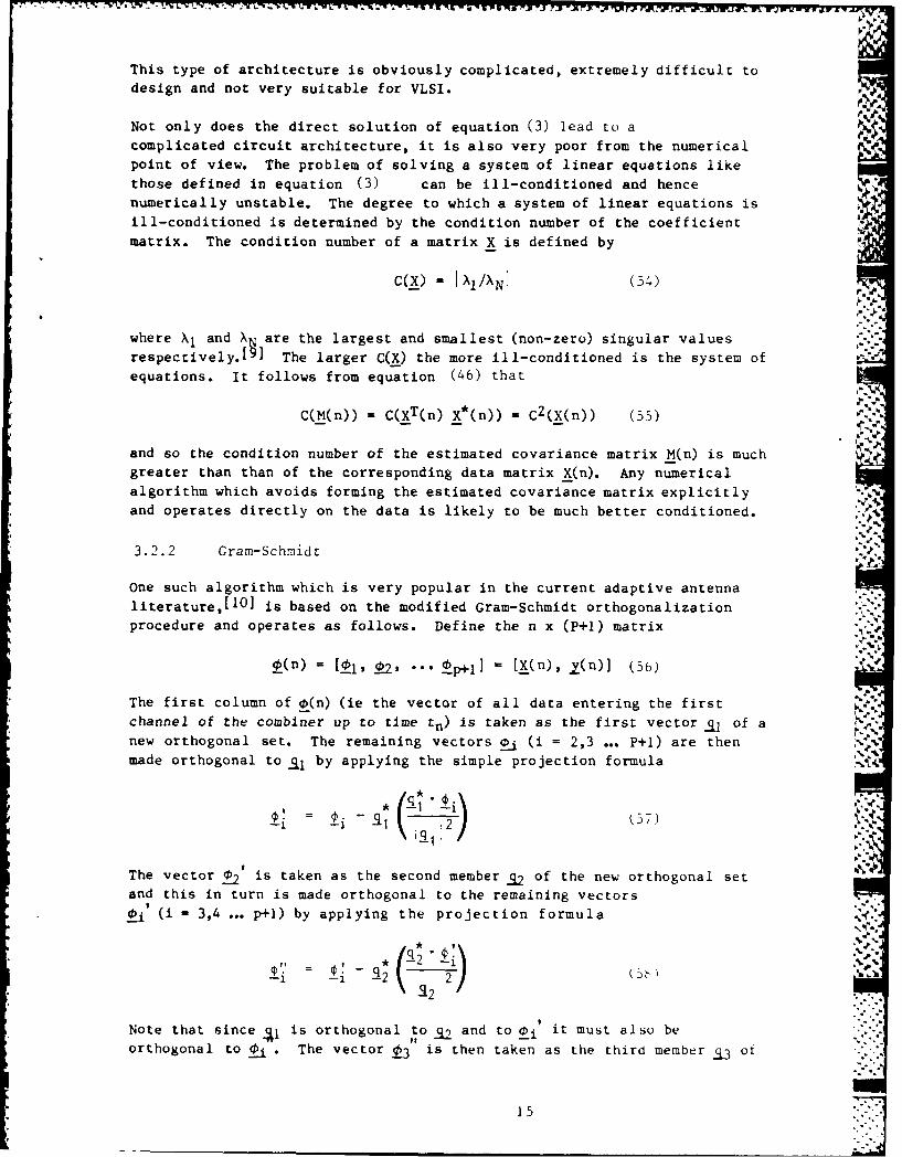
3.2.2 Gram-Schmidt

One such algorithm which is very popular in the current adaptive antenna

literature,[l 0 ] is based on the modified Gram-Schmidt orthogonalization

procedure and operates as follows. Define the n x (P+I) matrix

1(n) = i p2, -.. p+l] = [X(n), y(n)] (56)

The first column of 0(n) (ie the vector of all data entering the firstchannel of the combiner up to time tn) is taken as the first vector _a, of a

new orthogonal set. The remaining vectors 0 (i = 2,3 ... P+1) are then

made orthogonal to _/ by applying the simple projection formula

q Is,( -i*~ 537

The vector 0_2' is taken as the second member _q2 of the new orthogonal set %-p=.i

and this in turn is made orthogonal to the remaining vectors

±i' (i 3,4 ... p+l) by applying the projection formula

-2

Note that since is orthogonal to c 2 and to oi' it must also beorthogonal to 01 The vector 3 is then taken as the third member o.

15

the orthogonal set and the process is continued until a complete set of P+I

orthogonal vectors is obtained. Now the column vector .aP+I has been

constructed by adding to the vector y(n) a linear combination of the

columns in the matrix X(n). It must therefore be of the form

qp+l = X(n)w + y(n) (59)

which is identical to that of the general residual vector e(n) defined in 4

equation (50). Furthermore, since ap+l is orthogonal to the other

vectors q p and hence to the columns of X(n) it must in fact be the

residual vector for which E(n) = L1(n)JI is minimized. It therefore

provides the required output from the adaptive linear combiner.

In total the Modified Gram-Schmidt algorithm requires -4nP 2 real

multiplications and-4nP2 real additions ie-4P2 real multiplications and-4P2 real additions per sample time. The corresponding hardware

requirements and achievable throughout rates were discussed by Dillard in a

previous KTP3 report [il]

The modified Gram-Schmidt algorithm can also be applied to the general

adaptive antenna problem either by making use of the constraint

preprocessor technique described in section (3.1.2) or by solving the

Wiener-Hopf equation for the transformed data matrix

q(n) = q l 1 3 ...... (66)

Denoting the transformation from X(n) to Q(n) by

X(n)T(n) = Q(n) (61)

where T(n) is an upper triangular matrix, the constrained minimization

problem defined by equations (53) and (20) may be expressed as

follows. Minimize lle(n)l where

e(n) = Q(n) w' (62)

subject to the constraint that

s'Tw' = 3 (o3)

where

s T = sTT(n) (64)

The optimum weight vector w' is then given by the corresponding Wiener-Hopt \ "

equation

D(n) w* = s (65)-- - ' D-1I(b5) rJ'

s D (n)s' .

16 . i.

7. ..7

whe re

D(n) q (66)

Since Q(n) is o rthogonal, D(n) is a simple diagonal matrix and so equation(65) may be solved very easily. This approach was discussed during

our visit to the Hughes aircraft company who would seem to favour theModified Cram-Schmidt algorithm for many of their applications.

Of the two methods, the pre-processor technique should be more reliablesince the constraint is satisfied exactly before the adaptive weighting iscarried out and there is no need to solve for the weight vector explicitly.However, in situations where it is necessary to repeat the adaptive processfor a number of different look directions, the pre-processor method iscomputationally expensive because the entire Gram-Schmidt procedure must berepeated for each one. Solving equation (65) for each lookdirection is obviously more efficient for such applications.

The modified Gram-Schmidt algorithm described above is known to have goodnumerical properties.[121 However it does not lead to a particularlysuitable circuit architecture. This is due to the fact that theorthogonalization procedure is carried out column by column and so theentire data matrix X(n) must be obtained before the operation can commence.This of course leads to a considerable overhead in the amount of memory andcontrol circuitry which is required. It also means that as each new row ofdata is received, the entire procedure must be repeated in order to updatethe least-squares estimate. As a result the modified Gram-Schmidt tends tobe used on one block of data after another. It may be implemented usingthe type of triangular archtecture illustrated in Figure 15. On each cycleof the process each cell inputs two complete column vectors _ and andproduces the output vector 0_' where

,:- __ €- q (67)

An algorithm which operates row by row and can be implemented recursivelywould be much more suitable from the point of view of circuit architecture.For this reason the modified Gram-Schmidt algorithm is often computedapproximately using a technique which will be referred to as sequentialdecorrelation. [13]

3.2.3 Sequential Decorrelation

The sequential decorrelation process may also be carried out using a "

triangular array of processors as illustrated in figure 15. In this caseeach processor is a simple digital decorrelator which receives twocorrelated input sequences q(i) and 0(i) (i - 1,2 ... n). On each clockcycle it inputs the current values 0(i) and q(i) and produces the outputvalue

4€ (i) = (i) -q*(i)V(i) (be)

U i)

17

where

V(i) = V(i-1) + q*(i)(i) (69) .

and

U(i) = U(i-1) + q(i) 12 (70)

In this way each cell produces the output sequence

'(i) = $(i) - *(i) j)

* i) (7 1) "

Z Jq(j)12j=1

which is (asymptotically) uncorrelated with the input sequence q(i). Theoutput value o'(i) is passed southwards to the next cell on the next clock

cycle. From equation (71) it can be seen that in the sequentialdecorrelation process the value of 0'(i) is computed before the complete

sequence of data q(i) and 0(i) (i - 1,2 ... n) have been received and

before calculation of the correlation coefficient at time tn has beencompleted. As a result the output sequences 0'(i) and q(i) ki = I ... n)

are not truly orthogonalized as in the proper modified Gram-Schmidtalgorithm and the sequential decorrelation process is numerically inferior.

Particular case is need, for example, to avoid the problem which arises :"

when the denominator in equation (68) is identically zero duringinitial stages of the calculation. It is worth pointing out here that anexact recursive version of the Modified Gram-Schmidt algorithm has recently

been proposed by Ling and Proakis[21]. Their algorithm has not yet been

investigated for adaptive nulling but has much in common with the QRdecomposition technique described below and should perform similarly.

An exponentially fading memory can be incorporated into the sequentialdecorrelation algorithm by multiplying the terms U(n-1) and V(n-1) inequations (69) and (70) by a simple constant 0< 1. In this

more general form, the algorithm requires-8P2 real multiplications and

-6P 2 real additions per sample time. Since the sequential decorrelationprocess is computationally more expensive than the Modified Gram-Scmidt

technique and the QR decomposition algorithm which is described later, itwould appear to be of limited value for digital processing. However it iswell suited to analogue implementation since the basic cell function is

simply a correlation cancellation loop. The resulting analogue networkdoes not suffer from the fundamental problems of slow convergence

associated with closed loop analogue processors. .' *

The sequential decorrelation processor may also be applied to the generaladaptive antenna problem by using it in conjunction with a constraint

preprocessor of the type described in section 3.1.2.

18

3.2.4 QR Decomposition

On approach to the least squares estimation problem which is particularly

good from the numerical point of view is that of orthogonal

triangularization 1 4 ] otherwise known as QR decomposition. An n x n

orthogonal matrix Q(n) is generated such that

Q(n) X(n) (n)] (72)

where R(n) is a P x P upper triangular matrix. Then, since 2Q(n) isorthogonal we have

--w~n IiR(n)] u(n) (73E(n) IIQ(n)e(n)V Pn + L~n)(3

where

=) Q(n) y(n) (74)

It follows that the least-squares weight vector w(n) must satisfy the

equation

R(n) w(n) + u(n) = 0 (75)

and hence

E(n) - IIX(n)II (76)

Since the matrix R(n) is upper triangular, equation (75) is much

easier to solve than the Wiener-Hopf equation (3). The optimum wuight %'1

vector w(n) may be derived quite simply by back-substitution. Equation(75) is also much better conditioned since the condition number of

R(n) is given by

C(R(n)) = C(2(n)X(n)) = C(X(n)) (77)

This property follows directly from the fact that Q(n) is orthogonal. R(n)

is, in fact, the Cholesky square root factor of the covariance matrix M(n)

although it may be derived as shown here without actually forming thecovariance matrix explicitly.

,.

19 I-P

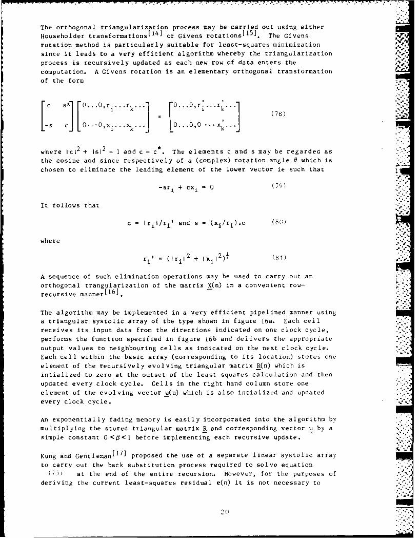
The orthogonal triangularization process may be carried out using either

Householder transformations[ 14] or Givens rotations[15] . The Givens

rotation method is particularly suitable for least-squares minimization

since it leads to a very efficient algorithm whereby the triangularization

process is recursively updated as each new row of data enters the

computation. A Givens rotation is an elementary orthogonal transformation

of the form

[c S:j[ .[...O.r. .. r [0o... O r>:1

where Ic 2 + Is1 2 = 1 and c = c . The elements c and s may be regarded as

the cosine and since respectively of a (complex) rotation angle 0 which is

chosen to eliminate the leading element of the lower vector ie such that

-sri + cxi 0 (79)

It follows that

c = Iril/r i ' and s =(xi/ri).c (8u)

where

ri (Iril2 + lxil2) (H)

A sequence of such elimination operations may be used to carry out an

orthogonal trangularization of the matrix X(n) in a convenient row-

recursive manner[16].

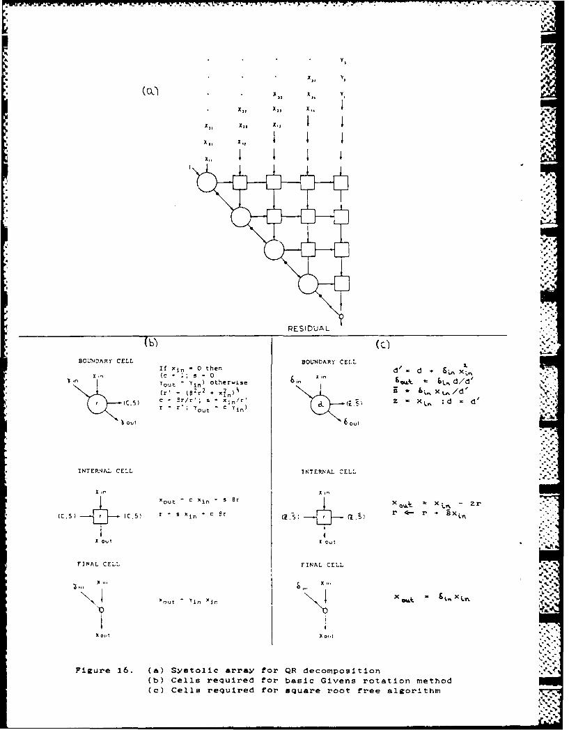
The algorithm may be implemented in a very efficient pipelined manner using

a triangular systolic array of the type shown in figure 16a. Each cell

receives its input data from the directions indicated on one clock cycle,

performs the function specified in figure 16b and delivers the appropriate

output values to neighbouring cells as indicated on the next clock cycle.

Each cell within the basic array (corresponding to its location) stores one

element of the recursively evolving triangular matrix R(n) which is

intialized to zero at the outset of the least squares calculation and then

updated every clock cycle. Cells in the right hand column store one

element of the evolving vector u(n) which is also intialized and updated

every clock cycle.

An exponentially fading memory is easily incorporated into the algorithm by

multiplying the stored triangular matrix R and corresponding vector u by a

simple constant 0<0<1 before implementing each recursive update.

Kung and Gentleman[1 7 ] proposed the use of a separate linear systolic array

to carry out the back substitution process required to solve equation

(75) at the end of the entire recursion. However, for the purposes of

deriving the current least-squares residual e(n) it is not necessary to

20

Y~ wa.--

compute the weight vector w(n) explicitly. McWhirter[16] has shown how

e(n) may be obtained in a very simple and direct manner which avoids the e

need to solve equation (75) at any stage of the process and leads to a

more reliable and efficient algorithm for recursive least-squares

minimization. The current least-squares residual e(n) is simply given by

e(n) = a(n) , Y(n) (S.-

where u(n) is the output which emerges from the bottom cell in the right

hand column of the systolic array in Figure 16 and Y(n) is the output

produced by the lowest boundary cell. The final cell indicated by means of -

a small circle in Figure 16 simply multiplies the completed product (n)

by the other parameter u(n) required to form the least squares residual

e(n).

Gentleman has derived a ve ry efficient square root free version of the

Givens rotation algorithm[' ]. It is not appropriate to describe it here

but the corresponding cell functions are given in figure 16c. In this

form, the QR decomposition algorithm (including fading memory) requires

-4P-+24P multiplications and -4P 2+14P real additions per sample time.

The adaptive linear combiner illustrated in Figure 16 enjoys all thedesirable architectural features of a systolic array. In particular it

does not require the block data storage which would be needed in order to

implement the modified Gram-Schmidt algorithm. As each row of data moves

down through the systolic array it is fully abosrbed into the statistical

estimation process, the triangular matrix R(n) is updated accordingly and

the corresponding residual is produced automatically. The circuit

architecture is enhanced by avoiding the need to derive an explicit

solution for the least-squares weight vector w(n). This leads to a

considerable reduction in the amount of computation and circuitry required

since it is no longer necessary to clock out each triangular matrix R(n),

carry out the back substitution or form the output linear combinationTx (n).(n). The adaptive linear combiner in Figure 16 is also based on avery stable and well-conditioned numerical algorithm. Indeed the method of

QR decomposition by Givens rotations is widely accepted as one of the verybest techniques for solving linear least squares problems. However the

final triangular linear system may, in general, be ill-conditioned and

avoiding the back-substituation process also enhances the numerical

properties of the adaptive combiner. In particular the circuit in Figure

lb produces the correct (zero) residual even if n<p and the matrix is not

of full rank. This sort of unconditional stability is most important in

the design of real time signal processing systems.

The systolic QR decomposition network may of course be applied to thegeneral adaptive antenna problem by using it in conjuction with a

constraint pre-processor of the type described in section 1 -2)Alternatively the constraint may be taken into account by solving a

transformed Wiener-Hopf equation analagous to that derived for the modified

Gram-Schmidt algorithm in section (3.2.2). The transformed dat.

matrix in this case is obtained by extracting the output residuals for each

of the sub array problems, ie for the first P-i elements, the first P-2

21

elements and so on. The constraint techniques as applied to the QR methodare so similar to those for Gram-Schmidt that no further discussion will be

given here.

A systolic array of the type described in this section is currently being

developed at the Standard Telecommunications Laboratories in Harlow for use

in an adaptive antenna test-bed system.fl9] The proposed system wasdescribed in some detail during the KTP-3 visit to STL. ,

3.2.5 The Hung and Turner Algorithm. 7

We conclude this section by reviewing briefly another novel direct solution

* algorithm which was recently proposed by Hung and Turner.[20 1 Their* algorithm is designed to be extremely efficient in situations where the

number of jamming sources J is known to be very much less than the numberof weighting coefficients P. The first J data snapshots (ie the first J

rows of the data matrix X) are assumed to span the space defined by the Jjammer response vectors and an orthonormal basis set for the space isgenerated by carrying out a Gram-Schmidt orthogonalization of the Jsnapshot vectors. The adaptive weight vector w is then obtained bysubtracting from the quiescent weight vectorw its projected component on

each of these basis vectors. The adapted weight vector should then beorthogonal to each of the J jammer signals as required.

In the Hung and Turner algorithm, the orthogonalizztion procedure is

carried out on the first J rows of the data matrix and not on the entire Pcolumns as with the modified Gram-Schmidt technique described in section(3.2.2). As a result, the total number of arithmetic operations

required is -8JP which is much less than than required for the modified

Gram-Schmidt algorithm when J<<P.

Hung and Turner have shown their method to be effective in the suppressionof many types of jammer sources and in the case of monotone point sources

the output jammer power is reduced to a few dB above the white noisebackground. Their method is bound to be numerically less stable and

accurate than the modified Gram-Schmidt or QR algorithms but it appearsnone the less to be very cost effective in the appropriate circumstances.

4 EFFECTS OF MfULTIPATH

In this section we will consider separately the effect of multipathpropogation on the jammer signals and on the desired signal.

4.1 Jammer Mlultipath.

Consider first a multipath jammer return which does not enter the main beam

or desired look direction of the array. If it is uncorrelated this returnappears as an additional jammer signal and simply absorbs another of theavailable degrees of freedom. If, on the other hand, the multipath return

* is fully correlated, the array can cancel both the jammer and its multipathby steering a single null in the appropriate vector balanced direction.

22

*-~ - ..- -... v.. . . . L.. ... .

Consider next the effect of a multipath jammer signal which enters the

array through the main beam or required look direction. If the multipathreturn is uncorrelated it cannot be cancelled by adaptive nulling. If the

return is correlated then it can at least be partially cancelled by the

adaptive algorithm. In the case of SLC the cancellation will be greatly

limited since the gain of the main antenna is assumed to be much greater

than that of the auxiliaries. For a general antenna array with a look

direction constraint the multipath signal can in principle be cancelled

completely depending on the gain assigned to the look direction.

In summary then, correlated multipath jammer returns cause less of a

problem than uncorrelated ones since they may be cancelled to some extent

without increasing the number of degrees of freedom in the system.

4.2 Signal Multipath. ..

The situation is reversed for signal multipath in which case correlated

returns cause a much greater problem that uncorrelated ones. Consider a

signal multipath return which enters the array along a path distinct from

the mian beam or required look direction. If this return is uncorrelated

it cannot cause any degradation of the desired signal and :ay be nulled

independently. It will simply absorb an additional degree of freedom in

the process. If the multipath signal is correlated, however, the effect

can be very damaging. In principle the multipath return could cancel the

desired signal completely. In the case of SLC the degradation will be

limited due to the high gain of the primary antenna. However, with a

general antenna array the degradation may be much more serious depending on

the gain which is chosen for the look direction. The only solution to thisproblem is to detect and elminate multipath signal returns before carrying

out any adaptive nulling. However, since the signal multipath returns are

often separated from the direct path by a very small angle, detecting and

eliminating them independently requires a high degree of spatial

resolution. This is one of the reasons why enhanced resolution algorithms

*[ are considered to be important and are discussed in the next section of

this report.

?r

I--

23

REFERENCES

1 Applebaum S P, Adaptive Arrays, IEEE Trans Ant and Prop, vol AP-24,

p 585 (1976).

2 Dokter R A, Masenten W K and Kinkel J F, "Trends in Adaptive Antenna

Circuit Design", Proc ELECTRO 79 (Feb 1979).

3 Widrow B, Mantey P E, Griffiths L J and Goode B B, "Adaptive Antenna

Systems", Proc IEEE, vol 55, p 2143 (1967).

4 Frost 0 L, "An Algorithm for Linearly Constrained Adaptive Array

Processing", Proc IEEE, vol 60, p 926 (1972)."A.

5 Griffiths L J, "A Simple Adaptive Algorithm for Real-Time Processing

in Antenna Arrays", Proc IEEE, vol 57, p 1696 (1969).

6 McWhirter J G, "Systolic Array for Recursive Least SquaresMinimization", Electronics Letters, vol 19, No 18, p 729 (Sept 1983).

7 Masenten W K, "Adaptive Signal Processing", IEE Seminar "Case Studies

in Advanced Signal Processing", Peebles, Scotland (Sept 1979).

8 Reed I S, Mallett J D and Brennan L E, "Rapid Convergence Rate in

Adaptive Arrays", IEEE Trans Aerosp Electron Syst, vol AES-10, p 853

(1974).

9 "Radar Signal Processing Architectures and Algorithms for VLSI", TTCP

Technical Panel KTP3, Technical Report TR-5.

10 "Adaptive Array Principles" by J E Hudson, Peter Peregrinus (1981).

11 "Dillard G M, "Processing Requirements for the Gram-Schmidt Procedure

Applied to a Digital Adaptive Array", TTCP Technical Panel KTP-3,

Technical Memo TM-T (June 1981).

12 Bjork A, "Solving Linear Least Squares Problems by Gram-SchmidtOrthogonalization", BIT, p 1 (1967).

13 "Introduction to Adaptive Arrays", by Monzingo R A and Miller T W,

Wiley Interscience (1980).'.-4.

14 Golub G, "Numerical Methods for Solving Linear Least SquaresProblems", Numerische Mathematik, vol 7, p 206 (1965).

15 Givens W, "Computation of Plane Unitary Rotations Transforming a

General Matrix to Triangular Form", J Soc Indust Appl Math, vol 6,

No 1, p 26 (1958).

16 McWhirter J G, "Recursive Least Squares Minimization using a Systolic

Array", Proc SPIE, vol 431, "Real Time Signal Processing VI" (1983).

2.

24 ..

17 Kung H T and Gentleman W M, "Matrix Triangularization by Systolic

Arrays", Proc SPIE, vol 298, Real Time Signal Processing IV" (1981).

18 Gentleman W M, "Least Square. Computations by Givens Rotations Without

Square Roots", J Inst Maths Applics, vol 12, p 329 (1973).

19 Ward C R, Robson A J, Hargrave P J and McWhirter J G, "Application ofa Systolic Array to Adaptive Beamforming", Proc lEE, vol 131, Pt F,

No 6 (1984).

20 Hung E K L and Turner R M, "An Adaptive Jammer Suppression Algorithmfor Large Arrays", McMaster University (1981).

21 Ling F and Proakis J G, "A Recursive Modified Gram-Schmidt Algorithmwith Application to Least Squares Estimation and Adaptive Filtering",

Proc IEEE conf ISCAS '84.

.2.-4 4% .*

" .3 -4

25"

JAMMING SIGNALS X

00 DESIREDSIGNAL

AUXILIARY .. aPRIMARY

CHA NNELS CHANNEL

W1 W 2 W3 W

OUTPUT SIGNAL

Figure 1. Adaptive side-lobe canceller

*_ -.-

WI W2 WN3 Wp

OUTPUT SIGNAL

Figure 2. General adaptive antenna array

w f2t

4 2 I W

~OUTPUT SIGNAL

Figure 3. AdaDtive combiner using real inputs

Y Y-' ' T7 -. I w-T

W6 WPL

6 6

6 6 8

WL WK

OUTPUT SIGNAL

Figure 4. Broad band adaptive antenna P.

MATRIX TRANSFORMATION,...-

A

OUTPUT SIGNAL

Figure 5. "Beam Space" adaptive combiner

AUXILIARY PRIMARY

Figure 6. Analogue correlation cancellation loop-., 0 SO

-- ~AXIIRE PRIMARY~'. .P!W'F J~T CANCELiiLOOPE

Figure 7. Use of multiple cancellation loops for SLC

V pth CHANNEL

x

I I ILOWI I IPASS

FILTER

+ Sp

I I MP

Figure 8.Use of multiple cancellation loops for general array

AUXILIARIES PRIMARY

WEIGHT W2 WEIGHT W~WEIGHUPDATE UPDATEUAE

0., RESIDUAL SIGNAL

Figure 9.LMS algorithm applied to SLC

x 2,uRESIDUAL

SIGNAL

UNIT

WEIGHT SETTING

Figure 10. Digital correlation cancellation loop

1-ALAEVCONSTRAINTEPR-POCS 1

4+

ADAPTIVE COMBINER

4-

4OUTPUT SIGNALFigure 12. Linear constraint pre-processor

*2 2w* r

AUXILIARIES

riLOW

IA D

OUPU SIGNALLWEIGHT

Figur 13. se ofhybri &hCOMPUeTATI oosfo L

fS

X~t)X (ti X~()Y /

.1 ** '~x

Lw

OU1U SIGNAL-Figue 13 Us of ybrd anlocu/d'italloos fo SL

OUPU

S

W,

OUTPT SGNA

S. Figure 15. Gram-Schmidt/Sequential decorrelation architecture

" 1

!Y,

x .•

I I . ° . °~

RESIDUAL ":]

I I %-..5.*

BOUNDOARY CELL BOUNDARY CELLn

If xin 0 then S.'nd X., .Xn (C -;S - 0 X- 'M

(.) c S r/r' ; s - xin/r' , = X . ;( = d ."r * r'; yourt C "in)

Z X,-d d

ou l "6 0. 1

INTER.NA.L CELL INTERJNAi, CELL .%

X ,m X ,

(C.S)(C.) r 9 s in "c Sr r[ r. x X

i ° i. -

X Oul 0.1lI'".

FINAL CELL FINAL CELL d = d

, x ... ,, x ,,w,Xiut Yin x6.i A,, x ,

XI

Figuxe 16. (a) Systolic array for QR decomposition

(b) Cells requied for basic Givens rotation method(c) Cells Xrequied for square root fee algoZithm

* (C) r c~ r* s c Brr 4 r%

%N:--

DOCUMENT CONTROL SHEET

Overall security classification of sheet Unclassified

(As far as possible this sheet should contain only unclassified information. If it is necessary to enlerclassified information, the box concerned must be marked to indicate the classification eg (P) (C) or (S)

V.-1. ORIC Reference (if known) 2. Originator's Reference 3. Agency Reference 4. Reori Security

Memorandum 3939 U/C Casian

5. Originator's Code (if 6. Originator (Corporate Author) lame and Locationknown)

Royal Signals and Radar Establishement

5a. Sponsoring Agency's 6a. Sponsoring Agency (Contract Authority) Name and Location "'"Code (if known)

7. Title

A Brief Review of Adaptive Null Steering Techniques

7a. Title in Foreign Language (In the case of iranslations)

7t. Presented at (for conference napers) Title, place and date of conference

B. Author 1 Surname, Initials 9(a) Author 2 9(b) Authors 3,4.... 10. Date pp. ref

McWhirter 3 G--'

11. Contract lumber 12. Period 13. Project 14. Other Reference

15. Distribution statement

Unlimited

Descriptors (or keywords)

continue on separate piece of p erA briet theoretical review of adaptive null steering is presented. The

Abstract basic theory is first outlined in the context of sidelobe cancellationsystems as well as general antenna arrays. Various approaches to the practicalimplementation of adaptive null steering are then disucssed. These fall intothe two main categories of closed loop mehtods and direct solution methods. Theclosed loop methods are very cost-effective and suitable in principal, foreither analogue or digital processing. However their rate of convergence isfundamentally limited and too slow for some applications. The direct solutionmethods do not suffer from this problem but tend to be suitable only for digitalprocessing and are more expensive from the computational point of view. Howeverthey are well suited to parallel processing and now provide a very practicalalternative due to recent advances in VLSI cirucit technology. A briefdiscussion on the effects of multi-path propagation on adaptive null steering

systems concludes this brief review.

S80/48

* -J. ~~**%~-. - - -- a -k k - -- - - - -

'p

p

F

~ ~ '%~7 -*~4----'* . ~ ' ' -. -.

4.~ ~ %. ~4.** '*4'~ * 4..- .-.-- ~-~ --