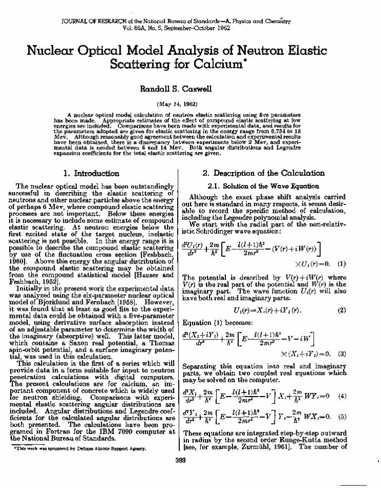
JOURNAL OF RESEARCH of the National Bureau of Standards—A. Physics and Chemistry Vol. 66A, No. 5, September-October 1962

Nuclear Optical Model Analysis of Neutron Elastic Scattering for Calcium*

Randall S. Caswell

(May 14, 1962)

A nuclear optical model calculation of neutron elastic scattering using five parameters has been made. Appropriate estimates of the effect of compound elastic scattering at low energies are included. Comparisons have been made with experimental data, and results for the parameters adopted are given for elastic scattering in the energy range from 0.734 to 18 Mev. Although reasonably good agreement between the calculation and experimental results have been obtained, there is a discrepancy between experiments below 2 Mev, and experi­mental data is needed between 6 and 14 Mev. Both angular distributions and Legendre expansion coefficients for the total elastic scattering are given.

1. Introduction

The nuclear optical model has been outstandingly successful in describing the elastic scattering of neutrons and other nuclear particles above the energy of perhaps 6 Mev, where compound elastic scattering processes are not important. Below these energies it is necessary to include some estimate of compound elastic scattering. At neutron energies below the first excited state of the target nucleus, inelastic scattering is not possible. In this energy range it is possible to describe the compound elastic scattering by use of the fluctuation cross section [Feshbach, I960]. Above this energy the angular distribution of the compound elastic scattering may be obtained from the compound statistical model [Hauser and Feshbach, 1952].

Initially in the present work the experimental data was analyzed using the six-parameter nuclear optical model of Bjorklund and Fernbach [1958]. However, it was found that at least as good fits to the experi­mental data could be obtained with a five-parameter model, using derivative surface absorption instead of an adjustable parameter to determine the width of the imaginary (absorptive) well. This latter model, which contains a Saxon real potential, a Thomas spin-orbit potential, and a surface imaginary poten­tial, was used in this calculation.

This calculation is the first of a series which will provide data in a form suitable for input to neutron penetration calculations with digital computers. The present calculations are for calcium, an im­portant component of concrete which is widely used for neutron shielding. Comparisons with experi­mental elastic scattering angular distributions are included. Angular distributions and Legendre coef­ficients for the calculated angular distributions are both presented. The calculations have been pro­gramed in Fortran for the IBM 7090 computer at the National Bureau of Standards.

2. Description of the Calculation

2.1 . Solution of the Wave Equation

Although the exact phase shift analysis carried out here is standard in many respects, it seems desir­able to record the specific method of calculation, including the Legendre polynomial analysis.

We start with the radial part of the non-relativ-istic Schrodinger wave equation:

d2Uj,(r) . 2m dr2 h2 [*-

l(l+iW 2mr2 -(V(r)+iW(r))j

X*7,(r)=0. (1)

The potential is described by V(r)-\-iW{r) where V{r) is the real part of the potential and W(r) is the imaginary part. The wave function Ui(r) will also have both real and imaginary parts:

Ul(r)=X,(r) + iYl(r).

Equation (1) becomes:

(2)

d2(Xl+iYl) 2m dr2 + fi2 [, l(l+iW

2mr2 •V-iwl

X(X,+iY,)=0. (3)

Separating this equation into real and imaginary parts, we obtain two coupled real equations which may be solved on the computer.

d2Xi , 2m

*This work was sponsored by Defense Atomic Support Agency.

dr2

d2Y,

h2

2m dr2 ' ft2

l{l+iW 2mr2

l(l + l)fi2

2mr2

-,] X,+^ WY,=0 (4)

'] V\Y,

ft

2 m ~\2 WXl=0. (5)

These equations are integrated step-by-step outward in radius by the second order Runge-Kutta method [see, for example, Zurmuhl, 1961]. The number of

389

integration steps is typically 100 to 500. If the wave functions become large, they are automatically re-normalized to smaller values by the code. The run­ning time for 15 Z's and 200 steps is about 1 min per energy including all angular distributions. The mass appearing in these equations is the reduced mass of the neutron in the neutron-nucleus center-of-mass system. The energy, E, is that of the neutron in the center-of-mass system. When the complex potential (V+iW) approaches a non-vanishing constant at the origin, then

Z7j(r)->C,r ,+1 as r->0 (6)

where d is a complex number independent of r [Amster, Leshan, and Walt, I960]. In the presence of the spin-orbit term (see below) there is a 1/r behav­ior of the potential energy for small values of r; how­ever, eq (6) still holds since this term is dominated by the 1/r2 dependence of the centrifugal potential [see Bohm, 1951]. Since the cross sections depend only on the logarithmic derivative of the wave function, the normalization is arbitrary and Ci can be taken to be any non-zero value. We have chosen k(l+i) for Ci where k is a small number chosen to prevent underflow or overflow problems. Provision is made in the code to calculate for values of I up to Z=29.

For the optical model parameters we have used a potential whose real and imaginary parts are:

2 rf A 1 dp r dr

W(r)=Ws (4a J ) = W S (4p2 exp [ ^ ] )

(7)

(8)

where

P(r) = 1

1+exp [̂ ] the usual "Saxon" potential; a is the strength of the spin-orbit interaction relative to the "Thomas" term for a nucleon; M is the neutron mass; Vc is the central real potential; Ws is the lowest value of

the imaginary surface potential; -^- is the Compton

wavelength for a nucleon; I is the orbital angular ->

momentum of the neutron; a is the Pauli spin oper­ator of the incident neutron; R0 is the nuclear radius; and a is the "diffuseness" parameter of the real potential. If the spin angular momentum of the incident neutron is parallel to the orbital angular momentum of the incident neutron, then j=1 + 1/2,

-+ ->

and a -1=1. If the spin and orbital angular mo--> ->

men turn are anti-parallel, then j=l —1/2 and a-l = — (Z + l ) . This leads to two real potentials, V+(r) and V~(r) corresponding to the parallel and anti-

-»-» parallel <r-l interactions. The wave equation is solved for each of these. To obtain the desired

cross sections, we need the phase shifts rj? and rjY which measure the effect of the complex potential on the neutron partial waves. These phase shifts are obtained by a calculation which compares the value for logarithmic derivative ft obtained by nu­merical integration in the presence of the nuclear potential with the corresponding quantity (Ai+iSi) for the zero phase shift spherical Hankel function solutions obtained in the absence of the nuclear potential.

The required expression for rjt is given by Blatt and Weisskopf [1952]:

vr-Jl-Al+iSl

For neutrons ft -iSl

exp (2£fj).

ro>. Gl(R)~-iFl(R)

^(2^=Gl(R)+iFl(Ry (10)

where Gt(R) and Ft(R) are solutions of eq (1) with (V(r)JriW(r))=0. In terms of spherical Bessel functions, Fl(x)=xji(x) and Gi(x)=xrii(x) where x=kR.

2.2. Evaluation of the Cross Sections Directly From the Nuclear Optical Model

The total cross section predicted by the nuclear optical model is made up of a shape-elastic scatter­ing cross section and a compound nucleus formation cross section [Feshbach, Porter, and Weisskopf, 1954]:

0"* = 0"e + 0"c.

However, the compound nucleus may decay into the entrance channel producing "compound elastic" scattering or it may produce inelastic scattering or charged particle reactions:

0"c = Gee ~\~ °V •

These equations may now be rearranged to sep­arate the elastic scattering (<rse and ace are not dis­tinguishable experimentally) from the reaction cross section:

°"« — ( ° " s e + <Tce) + 0> = <T e+ 0"r-

In the present calculation ace is estimated by the "fluctuation" cross section, aflJ which is important below energies of about 6 Mev:

When inelastic scattering and reactions are zero or negligible, the entire cross section is elastic:

In this case the fluctuation cross section may be obtained very simply from the phase shifts of the optical model alone (see Feshbach [1960] for a discus­sion of the fluctuation cross section).

390

We now proceed to evaluate the various cross sections from the calculated phase shifts (r?/s). For both incident particles and the nucleus without spin, the expressions for the incident plane wave, the total wave (which shows the effect of the potential of the nucleus on the incident wave), and the scat­tered wave are:

6<**=£2 ^ ^ ± i [}vt(kr)+hl(kr)]Pl{zose), 1=0 *

*to«(r) = S il ^ ± i [A?(Ar)+u,A,(Ar)]P,(coBtf), 1=0 *

(11)

(12)

and

^ B c a t t W = ^ t o t W — eik

1=0 * -l)A,(*r)P,(cos0). (13)

The incident neutrons which have spin 1/2 may be represented by a plane wave:

*inc=ef*%: (14)

where xlnc describes the spin wave function of the neutron. x i n c=(£) is spin "up . " Xtoc=(?) cor­responds to spin "down." In the presence of the nuclear potential the asymptotic form of the wave function of the neutron is:

r->oo V 'F(e)x„

where Fid) is the scattering matrix.

F(6)=A(d)+B(d)^n

(15)

(16)

where n is a unit vector perpendicular to the plane of [scattering. According to the Basel convention [Huber and Meyer, 1961], the positive direction of

-> polarization, given b}^ the unit vector n, is:

-» -»

\/Ci/\ rCf\

(17)

where kt and kf are the wave vectors of the incident and scattered neutrons.

In the equations above, h*=ji—ini and represents an incoming spherical wave and hi—ji+ini and repre­sents an outgoing spherical wave. To extend this treatment to the case of neutrons with spin incident on spin-zero nuclei [Lepore, 1950], we introduce the operators irt and TTJ which select the states for which j=l + ± and j=l~— \, respectively. These operators are

*-l *i

l + l + a-l A __l - 2[ + l a n d T r , - ^ ^ (17a)

K j = l + h T+ = l , T - = 0 . T f / = Z - i , 7T+ = 0, T- = 1. Applying our operators to the total wave function, eq (16) we have

lAtot=S 1=0

21 + 1 W++Tr-}[ht(kr)+rhhl(lcr)]

XPz(cos0)x lnc. (17b)

Let rjt and 77 r be phase shifts corresponding to the parallel and anti-parallel spin-orbit orientations for the neutron. At large radii we use the asymptotic form of the Hankel functions,

1=0

(21 2kT V 1 ^ 1

+ eAkr-(m)i])} XPz(cos0)x lnc. (17c)

If we now subtract the incident wave from the total wave to obtain the scattered wave, we find

a t t § 2 i Z r [ ( J + i ) ( i > , + - i ) + * 0 ? r - i )

+ ( i ? i + - ^ w ] * M c o s 0)xlnc, (18)

where we have used the expressions (17a) for the operators and the condition that when 7]f=rji = l, ^8Catt must equal zero. The right-left asymmetry in the scattering of a polarized beam is introduced

-> -» through the (a-1) operator:

( ^ l ) P , ( c o s ^ ) ^ . p ( - i ^ P , ( c o s 0)]-

Finally,

(19)

However, ^--=—sin 0 ^ -: ' be d (cos e)

(a • l)Pi(cos d) = (<r-n) i sin 0 i sii d(cos0)

Pz (cos 0) }

(<j-l)Pi(cos d) = (<T'n)iP](cosd).

where P}(cos 0)=sin 0

(20)

(21)

Pz(cos 0). Note: d(cos 0)

a (— l)m term is sometimes included in the definition of the associated Legendre function Pf (cos ^ 0), in which case our function has the opposite sign, and a minus sign appears on the right side of eq (21). A(d) and 5(0) appearing in the scattering matrix, eq (16) are:

^ ) = 2 ^ g [ ( / + D W - l ) + i W -1)]P,(COS0)

(22)

391

B(e)=~±[vt-vT]Pl(cose).

The differential scattering cross section is

da 1 dtt 2 trF+F=\A\2+\B\2.

The polarization is given by

2 Ee (A*B)

(23)

(24)

(25)

For a completely polarized incident beam with spin "up ," P=(L-R)/(L+R), where L and R are the measured left and right detector counting rates.

The total, compound nucleus formation, and shape elastic cross sections (integrated over angle) are:

* * = p 2 [ t f+ l )2 Re (l-vt) + l 2 Re (1 —nf)] (26) # z=o

' . = s S l(l+l)(l-\vf\2) + l(l-\v7\2)] (27) ft z=o

' . = p S l(l+l)\l-vt\2+m-vT\2]. (28) ft Z=0

For use in inelastic scattering calculations and in our estimate of compound elastic scattering, the "transmission coefficients" are also calculated:

n=ti- vT 2)andrr=(i-|^rl2). (29)

2.3. Compound Elastic Scattering

Whereas shape elastic scattering is given directly by the nuclear optical model, our estimate of com­pound elastic scattering is treated in four different ways depending upon the incident neutron energy. Below 3.35 Mev, it may be obtained from the optical model phase shifts, with a small correction for the

ENERGY (Mev)

SPIN, PARITY

4 . 4 a -3.90-*_ 3 . 7 3 -3 . 3 5 -

- I -. 2 + • 3 -• O - l -

0 +

F I G U R E 1. Low-lying energy levels of Ca40. Spins and parities in parentheses are taken from Troubetzkoy, Kalos, Lustig,

Kay, and Trupin [1961]. Levels taken as a continuum above 5 Mev.

observed (n, p) cross section. In the energy range from 3.35 to 5.0 Mev, a Hauser-Feshbach [1952] hand calculation using discrete energy levels of the target nucleus (see fig. 1) was made. From 5.0 to 5.7 Mev a Hauser-Feshbach calculation using a statistical-model residual nucleus was made. In this case the compound elastic scattering is isotropic because of the randomness of the spins and parities of the levels assumed in the statistical model. The angular isotropy has been proved by Wolfenstein [1951] and by Hauser and Feshbach. Above 6 Mev compound elastic scattering is neglected.

The fluctuation cross section, in the absence of inelastic scattering and reactions, may be obtained from the phase shifts of the optical model [Feshbach, I960]:

X[Pz(cos0)]2

l*l?«=4P S { ( l - | ^ | 2 ) + ( l - ! ^ | 2 ) } [ P K c o s W . (30)

At energies below the energy of the first excited state in the target nucleus (3.35 Mev for Ca40), we have used eq (30) to calculate the compound elastic scattering. Note that this leads not to isotropic scattering but to an angular distribution which goes predominantly as [Pz(cos 0)]2 for neutrons of angular momentum L

The cross section for inelastic scattering of a neutron of incident angular momentum Z, final angular momentum I', from a nucleus of initial angular momentum i and final angular momentum %' is given by Hauser and Feshbach as

1 er(l,i\l'^n=2(2:+1)^a(lja\l'j;\e) (31)

where

er(«,i|z/,i/|«=p(2Z+i)rI(S)S

Mhj\l',3'\<» (32)

and is the cross section for production of neutrons of energy Ef of angular momentum V, channel spin j ' , moving in a direction 0. The r index refers to possible channel spins, p to possible final neutron angular momenta, E'q to final neutron energies. J is the total angular momentum of the compound nucleus state. The prime on the summation indi­cates that we omit the term referring to the final neutron E', V', j ' we are considering. As we shall see the denominator of eq (32) is essentially the branching ratio of the specific neutron transition under consideration versus all other possibilities. If we immediately specialize to the case of compound elastic scattering, (E=E', 1=1', j=j'), consider spin zero nuclei only (j=j' = %9 i=0, and J = Z ± | ) , and Ti's as defined in eq (29), the angular distribution for the lih partial wave of compound elastically scattered

392

neutrons becomes:

(l+l)Tf(E) + ^'Tp(E'Q)/Tr(E)

P,Q,r

^( z4Nh)+ i lTj{E)

+ T,'T$(E',)ITT{E) P,Q,r

A>-s(l>l\l'l\e)}~ &V The A-functions that occur in eq (33) are easily expressed in terms of Z-coefficients used by Blatt and Biedenharn [1952] and tabulated by Biedenharn [1953]:

(34)

The question of phases does not enter since the Z-coefficient appears only when squared. Note that these results appear naturally in a Legendre series expansion which may be easily combined with the Legendre coefficient expansion as determined by the computer for the shape elastic scattering. Equa­tions (33) and (34) are used to calculate the region of discrete states of the target nucleus (3.35 to 5 Mev). A correction to the branching ratio appearing in eq (33) is applied to allow for experimentally observed reaction cross sections. From 5 to 5.7 Mev, the residual nucleus is considered as statistical, and the compound elastic scattering is isotropic.

2.4. Legendre Coefficient Analysis of the Elastic Scattering

The elastic scattering angular distribution is represented in the following way:

j fo ( g ^ ) = = ^ t o t a | e l a s t i c ^ {2l+ 1) S l(E)Pl (COS 6) (35)

where #>(#) = 1. The differential cross section as obtained from eq

(24) appears as a sum of the products of two series:

^ = S AlPl{co*d) S AmPm(cos6) all i m

+ S f t P i (cos 6) S B^Kcos 6). (36) l m

The first term in eq (36) may be represented by a single series of Legendre coefficients

^ = I > * A ( c o s 0 ) ,

where a* is given by

1=0 m=0

WU-wi+AO W(Z+m-ft) W 0 » - ?+*•)

a h(l+m+k)

Xl + m+k+l' (38)

where Cj= _ 1 . 3 . 5 . . . . ( 2 j - l )

; I, m are positive integers; j -

(l+m+k) is even; and \l—m\<k<l+m, that is, the three vectors satisfy the "triangle condition" [Whittaker and Watson, 1958).

The product of the two series in PJ(cos 6) can be reduced to product of two series in Pz(cos 6) which can then be solved by eq (38). First we express the P}( c o s 0)'s m terms of polynomial expansions in Pi(cos 6) [see Morse and Feshbach, 1953]:

PKcos0) = Hl + 1) '(2Z + 1) s in0

[Pl_1(cosd)-Pl+1{cosd)]

P ^ (cos 0)=sin <9[(2m—l)Pw_!(cos 6)

+ (2m-5)Pm_3(cos0)

+ (2m-9)Pm_5(cos0) +

(39)

.] (40)

(37)

Any product term P}(cos 0)P^(cos d) resulting from the series product in eqs (36) may be expressed in terms of a product of expressions from eqs (39) and (40). Note that in the product sin 6 cancels out, leaving only terms in Legendre polynomials, filia­tions (38 to 40) were programed for the computer so that a Legendre coefficient analysis of the form of eq (35) could be directly obtained from the calculated phase shifts.

The calculation could equally well be done through use of vector-coupling coefficients [Edmonds, 1957]. I t is expected that the problem for the computer would be about the same either way. The C3- coeffi­cients used here are closely related to the Clebsch-Gordan coefficient (ab00\abc0) as given in eq (5) of Blatt, Biedenharn, and Rose [1952].

3. Choice of Optical Model Parameters and Comparison With Experiment

Calcium is composed of 96.97 percent Ca40 with 2.06 percent of Ca44, and smaller amounts of Ca42, Ca43, Ca45, and Ca46. In this calculation it is con­sidered as pure Ca40 except that a slightly larger value of P 0 is used to approximate the effect of the other isotopes.

In the initial attempts to fit calcium neutron cross section data, the model of Bjorklund and Fernbach [1958] was used. The real potential is as described by eq (7), and the imaginary potential is a Gaussian absorption located at the surface:

W=WS exp \-(^^)T (41)

393

This model, which has been quite successful in fitting neutron elastic scattering data at 4.1, 7, and 14 Mev, involves six parameters: R0, Vc, a, a, Ws, and b. In attempting to fit this data, R0 was held constant at 1.25 A1/3 fermis, b at 0.980 fermis, a at 35. The aver­age atomic weight was used for A. The other three parameters were varied. A problem of the optical model is the large number of arbitrary parameters. In an attempt to reduce the number of parameters, the width of the surface absorption, b, was eliminated as an independent parameter and derivative surface absorption used instead as given in eq (8). Some­what surprisingly the agreement with the experimen­tal data was considerably improved at 14.6 Mev, and was equally good at the energies of 2 Mev and below where data existed which could be directly compared with optical model predictions using the fluctuation cross section. The improved agreement at 14.6 Mev may be stated in another way; namely, the value of b (0.980 fermis) is too small at this energy, and a thicker shell of surface absorption of neutrons should be used. This is given automatically by the use of a derivative surface absorption.

Using the derivative surface absorption model, RQ was held constant at 1.25A1/3 fermis, the value indicated by the work of Bjorklund and Fernbach, and also by the optical model analyses of proton polarization reported by Gursky and Stewart [1961]. Actually the parameters Vc and R0 act very much like a single parameter VcR0

n where n is equal to 2 at low energies and increases slightly with energy. Our choice is to hold R0 fixed and vary Vc. The strength of the spin-orbit coupling, a, was also held at the value of 35 used by Bjorklund and Fernbach because it was felt that changes or improvements in this value should come from the analysis of polar­ization data to which a is more sensitive, rather than angular distribution data which is considered here. Three parameters were allowed to vary, Vc, WB, and a. Although a could have been held fixed, independ­ent of energy, at a value of about 0.580 fermis to obtain fairly good fits to the experimental data everywhere, it was found that better fits were obtained if a was taken as 0.600 fermis at 14.6 Mev and at 0.550 fermis below 2 Mev. Smooth curves drawn through the data were used to obtain param­eters for the optical model calculations, even though local variations sometimes gave better fits (see fig. 2). This apparent jumping around of the experimental data is due at the low energies to the presence of resonances in the cross section, which the optical model averages over.

I t should also be mentioned that a calculation which predicts the energy variation of the param­eters of the optical model by use of a nonlocal potential has been made by Perey and Buck [1961]. The predictions of Perey and Buck have not been used here since it seemed unlikely that they would improve the cross section data.

Experimental data used for the parameter deter­mination at 14.6 Mev were taken from Cross and Jarvis [I960]; below 2 Mev, the data of Seagrave, Cranberg, and Simmons [1958] and Lane, Langs-

dorf, Monahan, and Elwyn [1960] as collected by Howerton [1961] were used. Comparison of the calculation to experimental data is shown in figures 3 through 12. Comparison is also made to data at

.600

.580

1 1 1 | I 1

. 560 - L^_____ 540 1 1 1 1 I 1

I | 1 1 1 | 1 1 1

a^—--^

1 1 1 1 1 1 1 1

| 1 1 l_

--

1 , , ," 1

-

I 0

1 1 I I 1 1 1 !

\ V c

1 1 1 1 1 1 1 1 4 8

1 1 | 1 1 1 1 1

w ^ ^ -

1 1 1 1 1 1 1 1 12 16

1 1 _

_

•^

1 1 20

2

NEUTRON ENERGY, Mev

F I G U R E 2. Optical model parameters versus energy as adopted for the calculation.

10,

en UJ

h-

o

.001

.0001

CALCIUM 14.6 M e v

40

9C

80

, DEGREES

120 160

F I G U R E 3. Elastic scattering at I4..6 Mev.

Experimental data are those of Cross and Jarvis [I960]. The curves in this and succeeding figures are from this calculation using the optical model param­eters of figure 2.

394

.10

c P 1.0 • o

o x> u>

\ </> c o

- Q

<s * 0.1 or Ld f -h-

< (J)

o f -

(/) < £Zi 0 I

.001

E 1

:

•

^V ^v

— —

—

i

~i i

f\

i i

r~

J

L_

~ 1 1 1 f CALCIUM 6.0 Mev

1 - * '-

1 1 1 1

—

-

—

,

—1

J — H

H i

— -\ J

—\

H

-̂

0 40 80 120 160 0 c m , DEGREES

F I G U R E 4. Elastic scattering at 6.0 Mev.

Experimental data are from Seagrave, Cranberg, and Simmons [1958].

4.1 Mev of Vincent, Morgan, and Prud'homme [1960] and to an angular distribution of Seagrave, Cranberg, and Simmons [1958] at 6.0 Mev. Neither of these distributions was used to obtain the optical model fit because the Hauser-Feshbach hand cal­culation involved made parameter fitting quite difficult (it later turned out that at 6.0 Mev the compound elastic scattering could be neglected). Nevertheless the agreement between calculation and experiment is about the same here as at the other energies. We may therefore be reasonably confident that the calculation predicts the cross sections quite well where they have not been measured.

I t would not be possible for these calculations to agree with both the Seagrave et al. and the Lane et al. experimental measurements, since these dis­agree with each other. In general the angular dis­tributions of Lane et al. are more isotropic, while the distributions of Seagrave et al. have a larger cross section in the forward direction. Somewhat more weight was given to the Seagrave et al. experi­ment, since the geometry appears to be somewhat cleaner and less subject to multiple scattering effects which would tend to make the distributions too isotropic.

This optical model underestimates the magnitude of the non-elastic (or compound nucleus formation) cross section at 14.5 Mev. The calculation gives

CALCIUM 4.1 Mev Exp. 4.02 Mev

.Oil 40 120 160 80

0 c m , DEGREES

F I G U R E 5. Elastic scattering at 4-02 Mev. The calculation is compared to the 4.1 Mev experimental data of Vincent,

Morgan, and Prud'homme [I960].

20 40 60 80 100 120

l f DEGREES 140 160

"* F I G U R E 6. Elastic scattering at 2.0 Mev.

Experimental data are from Seagrave, Cranberg, and Simmons (1958).

395

<

< - J

4 0 60 Be.

80 100 120 , , DEGREES

160 180

F I G U R E 7. Elastic scattering at 1.730 Mev.

Experimental data are from Lane, Lane, Langsdorf, Monahan, and Elwyn I960].

<

20 40 60 80 100 120 0c m , DEGREES

140 160

F I G U R E 8. Elastic scattering at 1.570 Mev.

Experimental data are from Lane, Langsdorf, Monahan, and Elwyn [I960].

1.227 barns at 14.6 Mev, whereas the experimental measurement at 14.5 Mev of Flerov and Talyzin [1956] gives 1.36 ±0.02 barns. This leads to a corresponding error in the total cross section, but does not affect the elastic cross section values. The total elastic cross section at 14.6 Mev is 0.803 barns, in agreement with the experimental value of 0.82 ±0.07 barns of Cross and Jarvis.

CO

<

60 80 100 120

0c .m . , DEGREES 140 160 180

F I G U R E 9. Elastic scattering at 1.250 Mev.

Experimental data are from Lane, Langsdorf, Monahan, and Elwyn [I960].

1.0,

0.1 en UJ

<

CO

<

.01

1 1 1 CALCIUM 1.005 Mev

60 80 100 120

0c.m>f DEGREES 140 160 180

F I G U R E 10. Elastic scattering at 1.005 Mev.

Experimental data are from Lane, Langsdorf, Monahan, and Elwyn [1960] at 1.01 ± 0.03 Mev (crosses) and from Seagrave, Cranberg, and Simmons [1958] at 1.0 Mev (vertical lines).

4. Results of the Calculation

The calculated angular distributions for total elastic scattering are given in table 1 and the Legendre coefficient expansions are given in table 2.

396

t= r

? oil

<

in <

.01

n 1— CALCIUM 0.930 Mev

_L 20 4 0 60 140 160 180 80 100 120

0c.m.f DEGREES

F I G U R E 11. Elastic scattering at 0.930 Mev. Experimental data are from Lane, Langsdorf, Monahan, and Elwyn [I960].

T A B L E 1. Angular distributions of neutron elastic scattering for calcium (barns/steradian)

Angle

deq 0. 5.0 10.0 15.0 20.0

25.0 30.0 35.0 40.0 45.0

50.0 55.0 60.0 65.0 70.0

75.0 80.0 85.0 90. 0 95.0

100.0 105.0 110.0 115.0 120.0

125.0 130.0 135.0 140.0 145.0

150.0 155. 0 160.0 165.0 170.0 175.0 180.0

18. 000 Mev

2.2740 2.1104 1. 6774 1.1189 0. 5980

.2290

.0439

.0031

.0349

.0755

.0914

.0792

. 0527

.0281

.0142

.0112

.0141

.0174

.0178

.0152

.0110

.0072

.0049

.0040

.0039

.0038

.0033

.0028

.0026

.0029

.0035

.0043

.0048

.0049

.0045

.0040

.0038

17.100 Mev

2.1727 2. 0223 1. 6223 1.1011 0.6068

.2467

.0558

.0037

.0270

.0657

.0847

.0772

.0540

.0302

.0152

.0106

.0127

.0161

.0173

.0156

.0121

.0086

.0061

.0048

.0042

.0038

.0032

.0028

.0029

.0035

.0044

.0052

. 0053

.0048

.0039

.0030

.0026

16.300 Mev

1. 9827 1. 8512 1.4995 1. 0364 0. 5893

.2544

.0677

.0084

.0232

.0582

.0787

.0753

.0556

.0330

.0175

.0117

.0129

.0161

.0179

.0170

.0143

.0113

.0088

.0072

.0059

.0047

.0036

.0031

.0035

.0048

.0064

.0076

.0075

.0063

.0043

.0026

.0019

15. 500 Mev

1.8448 1. 7277 1. 4131 0. 9947 .5842

.2684

.0837

.0161

.0212

.0507

.0712

.0712

. 0553

.0350

.0197

.0123

.0128

.0154

.0174

.0175

.0160

.0139

.0119

.0099

.0079

.0057

.0038

.0031

.0039

.0059

.0083

.0099

.0097

.0077

.0047

.0021

.0010

14. 750 Mev

1. 7511 1. 6449 1.3584 0. 9740 .5908

.2884

.1029

.0261

.0208

.0437

.0632

.0660

.0541

.0366

.0220

.0142

.0127

.0143

.0164

.0175

.0174

.0166

.0152

.0130

.0100

.0067

.0041

.0030

.0041

.0069

.0101

.0121

.0117

.0090

.0051

.0017

.0004

14.000 Mev

1. 6825 1. 5857 1.3234 0. 9678 .6074

.3147

.1262

.0384

.0212

.0366

.0545

.0600

.0523

.0377

.0237

.0147

.0113

.0117

.0139

.0162

.0179

.0184

.0175

.0150

.0113

.0071

.0039

.0027

.0039

.0071

.0105

.0126

.0122

.0093

.0051

.0015

.0000

13.300 Mev

1. 5868 1. 5013 1.2685 0.9495 .6203

.3451

.1585

.0614

.0310

.0354

.0479

.0533

.0484

. 0371

.0251

.0162

.0118

.0111

.0130

.0162

.0194

.0217

.0219

.0196

.0150

.0093

.0047

.0028

.0043

.0085

.0131

.0161

.0157

.0120

.0067

.0020

.0001

0.1

< V (/) o h-

<

"1 ZJ CALCIUM 0.770 Mev

20 40 60 80 0c

100 120 , DEGREES

180

F I G U R E 12. Elastic scattering at 0.770 Mev. Experimental data are from Lane, Langsdorf, Monahan, and Elwyn [I960].

T A B L E 1. Angular distributions of neutron elastic scattering for calcium (barns I steradian)—Continued

Angle

deg 0. 5.0 10.0 15.0 20.0

25.0 30.0 35.0 40.0 45.0

50.0 55.0 60.0 65.0 70.0

75.0 80.0 85.0 90.0 95.0

100.0 105.0 110.0 115.0 120.0

125.0 130.0 135.0 140.0 145.0

150.0 155.0 160.0 165.0 170.0

175.0 180.0

12. 700 Mev

1.5352 1.4571 1.2434 0. 9480 .6382

.3726

.1848

.0792

.0382

.0345

.0434

.0491

.0466

.0373

.0259

.0163

.0105

.0089

.0108

.0148

.0193

.0226

.0233

.0209

.0158

.0097

.0047

.0027

.0042

.0083

.0130

.0159

.0156

.0121

.0070

.0025

.0007

12.100 Mev

1.4533 1.3852 1.1979 0. 9357 .6555

.4078

.2238

.1109

.0573

.0416

.0428

.0459

.0441

.0368

.0268

.0171

.0105

.0079

.0096

.0144

.0205

.0255

.0274

.0252

.0194

.0121

.0059

.0032

.0048

.0096

. 0152

.0188

.0186

.0146

.0086

.0034

.0013

11. 500 Mev

1.4105 1.3492 1.1794 0. 9393 .6781

.4410

.2577

.1378

.0739

.0489

.0439

.0446

.0428

.0362

.0264

.0164

.0091

.0061

.0078

.0131

.0198

.0254

.0276

.0255

.0197

.0124

.C063

.0035

.0049

.0094

.0146

.0179

.0178

.0143

.0089

.0042

.0023

10. 900 Mev

1.3773 1.3219 1.1679 0. 9476 .7039

.4768

.2945

.1684

.0947

.0599

.0480

.0448

.0417

.0352

.0256

.0155

.0079

.0046

.0063

.0119

.0189

.0247

.0271

.0252

.0197

.0127

.0069

.0042

.0053

.0093

.0139

.0168

.0168

.0137

.0090

.0048

.0032

10.400 Mev

1.3298 1.2816 1.1470 0.9521 .7321

.5212

.3445

.2143

.1302

.0832

.0604

.0497

.0426

.0345

.0247

.0148

.0073

.0042

.0062

.0123

.0202

.0269

.0298

.0281

.0223

.0149

.0086

.0057

.0068

.0109

.0158

. 0190

.0188

.0154

.0103

.0058

.0040

9.890 Mev

1.3199 1.2756 1.1511 0. 9692 .7609

.5571

.3815

.2470

.1553

.0997

.0695

.0535

.0431

.0334

.0232

.0134

.0063

.0035

.0057

.0117

.0193

.0257

.0285

.0270

.0218

. 0151

.0095

.0067

.0076

.0111

.0152

.0178

.0176

.0145

.0100

.0061

.0046

9.410 Mev

1.3476 1.3061 1.1891 1.0165 0.8159

.6152

.4370

. 2946

.1916

.1240

.0830

.0588

.0433

.0312

.0205

.0113

.0051

.0032

.0059

.0121

.0196

.0257

.0284

.0269

.0221

.0158

.0106

.0081

.0090

.0122

.0159

.0182

.0179

.0149

.0106

.0069

.0055

397

T A B L E 1. Angular distributions of neutron elastic scattering for calcium (barns/steradian)—Continued

Angle

deg 0. 5.0 10.0 15.0 20.0

25.0 30.0 35.0 40.0 45.0

50.0 55.9 60.0 65.0 70.0.

75.0 80.0 85.0 90.0 95.0

100.0 105.0 110.0 115.0 120.0

125.0 130.0 135.0 140.0 145.0

150.0 155.0 160.0 165.0 170.0

175.0 180.0

Angle

deg 0. 5.0 10.0 15.0 20.0

25.0 30.0 35.0 40.0 45.0

50.0 55.0 60.0 65.0 70.0

75.0 80.0 85.0 90.0 95.0

100.0 105.0 110.0 115.0 120.0

125.0 130.0 135.0 140.0 145.0

150.0 155.0 160.0 165.0 170.0

175.0 180.0

8.950 Mev.

1.3531 1.3142 1.2039 1.0400 0. 8472

.6513

.4736

.3276

.2182

.1429

.0946

.0645

.0450

.0308

.0193

.0102

.0045

.0030

.0058

.0118

.0188

.0245

.0270

.0258

.0215

.0161

.0116

.0094

.0100

.0127

.0157

.0174

.0168

.0141

.0103

.0071

.0058

6.300 Mev.

1.5013 1. 4726 1.3897 1.2617 1.1018

0. 9254 .7473 .5799 .4321 .3086

.2105

.1363

.0828

.0463

.0231

.0102

.0049

.0050

.0086

.0138

.0190

.0231

.0255

.0260

.0252

.0239

.0229

.0227

.0233

.0242

.0251

.0252

.0244

.0229

.0210

.0196

.0190

8.510 Mev.

1.3565 1.3211 1.2203 1.0692 0.8887

.7014

.5265

.3775

.2603

.1746

.1156

.0763

.0500

.0316

.0183

.0090

.0039

.0032

.0065

.0125

.0193

.0247

.0271

.0260

.0223

. 0174

.0132

.0112

.0116

.0137

.0162

.0175

.0169

.0143

.0108

.0079

.0067

6.000 Mev.

1. 5253 1. 4980 1. 4188 1.2958 1.1409

0. 9681 .7910 .6219 .4697 .3398

.2345

. 1531

.0935

.0524

.0262

.0117

. 0058

.0060

.0098

.0152

.0207

.0249

.0274

.0282

.0277

.0267

.0259

.0256

.0261

.0270

.0278

.0280

.0276

.0265

.0252

.0241

.0237

8.100 Mev.

1.3728 1.3389 1.2422 1.0962 0. 9205

.7358

.5608

.4087

.2861

.1939

.1284

.0835

.0531

.0323

.0179

.0085

.0036

.0032

.0065

.0123

.0186

.0236

.0259

.0251

.0220

.0179

.0144

.0126

.0129

.0146

.0164

.0173

.0165

.0140

.0109

.0083

.0073

5.700 Mev.

1. 5377 1. 5109 1.4335 1.3128 1.1604

0. 9894 .8134 .6439 .4902 .3580

.2497

.1654

.1031

.0597

.0318

.0160

.0093

.0089

.0122

.0173

.0225

.0268

.0295

.0307

.0309

.0305

.0302

.0304

.0311

.0322

.0332

.0337

.0336

.0329

.0319

. 0311

.0308

7.700 Mev.

1.4119 1.3795 1.2867 1.1457 0.9741

.7911

.6141

.4565

.3257

.2237

.1485

.0952

. 0585

.0338

.0175

.0078

.0034

.0037

.0075

.0135

.0196

.0243

.0264

.0257

.0228

.0191

.0161

.0146

.0150

.0165

.0181

.0187

.0178

.0155

.0125

.0101

.0091

5.430 Mev.

1. 5673 1.5411 1.4651 1.3464 1.1956

1.0255 0.8489 .6774 .5202 .3835

.2704

.1813

.1149

.0683

.0383

.0213

.0139

.0132

.0166

.0217

.0271

.0315

.0344

.0359

.0364

.0363

.0363

.0368

.0378

.0390

.0403

.0411

.0414

.0411

.0406

.0401

.0399

7.330 Mev.

1.4324 1.4010 1.3108 1.1732 1.0046

0.8231 .6457 . 4853 .3500 .2426

.1617

.1034

.0628

.0356

.0180

.0078

.0035

.0038

.0076

.0132

.0190

.0235

.0255

.0251

.0229

.0199

.0174

.0162

.0165

.0177

.0189

.0192

.0182

.0160

.0133

.0111

.0103

5.160 Mev.

1. 5719 1. 5464 1. 4723 1. 3563 1.2087

1.0414 0. 8669 .6966 .5395 .4019

.2872

.1961

.1276

.0791

.0474

.0290

.0206

.0191

.0218

.0265

.0317

.0361

.0393

.0412

.0423

.0429

.0435

.0446

.0460

.0477

.0494

.0508

. 0516

.0519

. 0518

. 0517

. 0516

6.970 Mev.

1.4620 1.4320 1.3456 1.2131 1.0491

0.8704 .6930 .5294 .3882 .2731

.1839

.1180

.0713

.0397

.0196

.0084

.0039

.0046

. 008?

.0145

.0203

.0247

.0267

.0264

.0245

.0219

.0198

.0189

.0193

.0204

.0216

.0218

.0208

.0188

.0163

.0143

.0135

4.910 Mev.

1. 6092 1. 5837 1. 5096 1.3935 1.2453

1.0770 0. 9006 .7276 .5671 .4254

.3065

.2113

.1392

.0877

.0538

.0340

.0247

.0227

.0250

.0295

.0344

.0388

.0422

.0447

.0468

.0489

.0515

.0551

.0595

.0649

.0707

.0767

.0824

.0872

.0910

.0933

.0941

6.663 Mev.

1.4826 1.4533 1.3687 1.2385 1. 0766

0.8990 .7211 .5554 .4106 .2910

.1972

.1270

.0768

.0427

.0211

.0091

.0043

.0048

.0087

.0142

.0197

.0239

.0261

.0262

.0248

.0229

.0213

.0207

.0212

.0222

.0231

.0232

.0223

.0204

.0183

. 0165

.0159

4.670 Mev.

1. 6033 1. 5786 1. 5064 1.3932 1.2483

1.0832 0. 9097 .7387 .5792 .4377

.3181

.2218

.1481

.0951

.0598

.0386

.0282

. 0252

.0268

.0306

.0352

.0395

.0430

.0459

.0486

.0515

.0551

.0597

.0653

.0719

.0791

.0864

.0934

.0994

. 1042

.1072

. 1082

T A B L E 1. Angular distributions of neutron elastic scattering for calcium {barns/steradian)—Continued

Angle

deg 6. 5.0 10.0 15.0 20.0

25.0 30.0 35.0 40.0 45.0

50.0 55.0 60.0 65.0 70.0

75.0 80.0 85.0 90.0 95.0

100.0 105.0 110.0 115.0 120.0

125.0 130.0 135.0 140.0 145.0

150.0 155.0 160.0 165.0 170.0

175.8 180.0

Angle

deg 0. 5.0 10.0 15.0 20.0

25.0 30.0 35.0 40.0 45.0

50.0 55.0 60.0 65.0 70.0

75.0 80.0 85.0 90.0 95.0

100.0 105.0 110.0 115.0 120.0

125.0 130.0 135.0 140.0 145.0

150.0 155.0 160.0 165.0 170.0

175.0 180.0

4.440 Mev

1. 7219 1. 6938 1. 6118 1.4832 1.3190

1.1321 0. 9366 .7455 .5696 .4170

.2923

.1972

.1304

.0884

.0665

.0589

.0600

.0648

.0691

.0702

.0668

.0590

.0481

.0363

.0261

.0201

.0201

.0277

.0430

.0654

.0933

.1243

.1555

.1839

.2066

.2212

.2262

2.970 Mev

1.4990 1. 4793 1.4218 1. 3311 1. 2143

1. 0797 0. 9364 .7927 .6558 .5311

.4219

.3298

.2550

.1962

.1520

.1201

.0988

.0858

.0795

.0782

.0803

.0848

.0908

.0981

.1068

.1176

.1316

.1498

.1727

.2006

.2326

.2671

.3015

.3329

.3580

.3743

.3800

4.230 Mev

1. 6126 1. 5889 1. 5197 1.4109 1.2710

1.1107 0. 9408 .7719 .6126 .4698

.3475

.2477

.1703

.1138

.0754

.0519

.0396

.0352

.0358

.0390

.0432

.0475

.0514

.0552

.0591

.0637

.0693

.0762

.0846

.0942

.1047

.1156

.1261

.1354

.1428

.1475

.1491

2.690 Mev

1. 3767 1.3603 1. 3123 1. 2361 1.1369

1.0211 0. 8957 .7679 .6440 .5290

.4269

.3396

.2682

.2119

.1694

.1387

.1175

.1036

.0949

.0900

.0879

.0882

.0910

.0968

.1063

.1202

.1391

.1632

.1922

. 2252

.2607

. 2967

. 3309

. 3608

. 3841

. 3988

. 4039

4.020 Mev

1. 5996 1. 5765 1. 5093 1.4034 1.2672

1.1109 0.9449 .7794 .6229 .4818

.3602

.2604

.1823

.1247

.0850

.0600

.0464

.0408

.0404

.0428

.0464

.0504

.0545

.0587

.0636

.0694

.0765

.0852

.0956

.1075

.1206

.1341

.1473

.1592

.1686

.1747

.1768

2.440 Mev

1. 2546 1. 2405 1.1991 1.1332 1.0473

0.9466 .8374 .7253 .6160 .5138

.4220

.3426

.2764

.2230

.1814

.1500

.1268

.1102

.0986

.0908

.0862

.0846

.0863

.0917

.1016

.1168

.1375

.1640

.1957

.2315

.2698

.3084

.3448

.3765

.4011

.4167

.4220

3.820 Mev

1. 6072 1. 5836 1. 5150 1.4077 1.2712

1.1161 0. 9528 .7907 .6370 .4971

.3749

.2727

.1915

.1312

.0900

.0651

.0524

.0479

.0476

.0491

.0511

.0534

.0567

.0616

.0684

.0769

.0865

.0968

.1078

.1198

. 1335

.1491

.1662

.1834

.1982

.2085

.2121

2.210 Mev

1.1456 1.1334 1. 0975 1.0403 0. 9656

.8779

.7822

. 6838

.5873

.4964

.4142

.3425

.2818

.2321

.1924

.1614

.1376

.1196

.1061

.0962

.0896

.0864

.0870

.0920

.1021

.1181

.1403

.1686

.2025

.2407

.2814

.3223

.3608

.3943

.4202

.4366

.4422

3.640 Mev

1.3986 1.3787 1.3208 1.2298 1.1132

0.9799 .8394 .7006 .5708 .4559

.3592

.2824

.2250

.1854

.1607

.1475

.1421

.1409

.1410

.1401

.1366

.1301

.1204

.1083

.0948

.0808

.0677

.0562

.0474

.0417

.0392

.0397

.0425

.0464

.0505

.0534

.0545

2.000 Mev

1.0433 1.0327 1.0017 0. 9522 .8873

.8111

.7278

.6417

.5569

.4767

.4036

.3391

.2839

.2380

.2005

.1704

.1465

.1276

.1127

.1013

.0933

.0889

.0885

.0930

.1032

.1196

.1426

.1720

.2071

.2466

.2885

.3305

. 3699

. 4041

. 4304

. 4471

. 4529

3.460 Mev

1.5570 1. 5360 1.4746 1.3776 1.2522

1.1074 0. 9525 .7966 .6475 .5115

.3927

.2936

.2148

.1552

.1129

.0850

.0685

.0602

.0574

.0579

.0601

.0634

.0675

.0725

.0791

.0877

.0987

.1126

.1293

.1485

.1696

.1915

.2128

.2319

.2471

.2568

.2602

1.810 Mev

0.9309 .9221 .8963 .8552 .8013

.7378

.6881

.5958

.5241

.4554

.3919

.3349

.2851

.2424

.2065

.1767

.1520

.1315

.1148

.1015

.0916

.0856

.0841

.0878

.0974

.1133

.1358

.1645

.1986

.2367

.2770

.3172

.3550

.3877

. 4130

.4290

. 4345

3.290 Mev

1. 5703 1. 5497 1.4896 1.3944 1.2711

1.1283 0.9751 .8206 .6726 .5375

.4195

.3208

.2421

.1822

.1390

.1098

.0917

.0817

.0774

.0768

.0783

.0813

.0855

.0912

.0990

.1096

.1239

.1423

.1647

.1907

.2191

.2484

.2765

.3013

.3207

.3331

.3374

1.630 Mev

0. 8244 .8173 .7963 .7628 .7187

.6663

.6083

.5476

.4867

.4280

.3731

.3232

.2789

.2403

.2071

.1787

.1544

.1337

.1163

.1019

.0909

.0837

.0811

.0839

.0926

.1078

.1296

.1575

.1905

.2274

.2661

.3044

. 3400

. 3706

. 3941

. 4089

. 4139

398

T A B L E 1. Angular distribution of neutron elastic scattering for calcium (barnsI'steradian)—Continued

Angle

deg 0. 5.0 10.0 15.0 20.0

25.0 30.0 35.0 40.0 45.0

50.0 55.0 60.0 65.0 70.0

75.0 80.0 85.0 90.0 95.0

1.480 Mev

0.4400 .4365 .4263 .4097 .3879

.3619

.3330

. 3025

.2717

.2416

.2131

.1868

.1630

.1418

.1230

.1066

.0922

.0797

.0689

.0600

1.340 Mev

0. 6742 .6691 .6541 . 6301 .5982

.5602

.5178

.4730

.4275

.3829

.3404

.3007

.2646

.2319

.2028

.1769

.1540

.1338

.1163

.1016

1.210 Mev

0.3484 .3459 .3388 .3273 .3121

.2938

.2733

.2515

.2292

.2071

.1857

.1655

.1467

.1295

.1139

.0998

.0871

.0758

.0659

.0576

1.096 Mev

0.3193 .3172 .3111 .3013 .2883

.2726

.2550

.2360

.2165

.1969

.1778

.1596

.1424

.1264

.1117

.0983

.0861

.0752

.0656

.0575

0.991 Mev

0. 2848 .2831 .2780 .2697 .2586

.2453

.2302

.2140

.1972

.1802

.1636

.1477

. 1325

.1184

.1053

.0932

.0822

.0723

.0636

.0562

0,853 Mev

0.4682 .4656 .4577 .4450 .4280

.4074

.3842

.3590

.3328

.3063

.2801

.2548

.2306

.2078

.1865

.1669

.1489

.1326

. 1182

.1060

0.734 Mev

0. 4299 .4277 .4211 .4104 .3960

.3786

.3588

.3372

.3146

.2915

.2685

.2460

.2244

.2038

.1844

.1664

.1498

.1348

. 1215

.1100

T A B L E 1.—Angular distribution of neutron elastic scattering for calcium (barns/steradian)—Continued

Angle

dea 100.0 105.0 110.0 115.0 120.0

125.0 130.0 135.0 140.0 145.0

150.0 155.0 160.0 165.0 170.0

175.0 180.0

1.480 Mev

.0530

.0484

.0464

.0476

.0521

.0603

.0720

.0872

.1051

.1250

.1459

.1666

.1858

.2022

.2148

.2228

.2255

T.340 Mev

.0902

.0824

.0790

.0805

.0875

.1003

.1188

.1426

.1709

.2023

.2352

.2677

.2978

.3236

.3435

.3560

.3602

1.210 Mev

.0511

.0465

.0443

.0447

.0480

.0542

.0634

.0752

.0893

.1049

.1212

.1373

. 1523

.1651

.1749

.1810

.1831

1.096 Mev

.0511

.0465

.0441

.0441

.0467

.0519

.0598

.0699

.0820

.0955

.1095

.1234

.1363

.1473

.1557

.1610

.1628

0.991 Mev

.0503

.0461

.0437

.0435

.0456

.0499

.0565

.0652

.0755

.0869

.0989

.1108

.1218

.1312

.1384

.1429

.1445

0.853 Mev

.0961

.0889

.0847

.0839

.0866

.0930

.1028

.1157

.1312

.1484

.1665

.1844

.2010

.2152

.2261

.2329

.2352

9.734 Mev

.1007

.0937

.0894

.0878

.089a

.0937

.1010

.1108

.1227

.1360

.1501

.1640

.1768

.1879

.1963

.2016

.2034

T A B L E 2. Legendre coefficients for calcium elastic scattering

Energy.. . Mev _ Total elastic barns. _ Si(E),l= 0

1 2 3 4 5

6... 7__. 8 9 10 11 12 13 14 15

18.000 0.836 1.00000 0.80315 . 63456 .52042 .44965 .38692

.33349

. 27457

.19745

.11379

.04970

.01833

.00600

.00176

. 00048

.00012

17.100 0.826 1.00000 0. 79852 . 63283 . 52075 . 44827 . 38273

. 32659

. 26459

. 18289

. 10103

. 04153

. 01441

. 00448

.00125

. 00033

.00008

16. 300 0.806 1.00000 0. 77512 . 61087 . 50234 . 43098 . 36377

. 30864

. 24661

. 16280

.08647

. 03233

. 01021

. 00294

. 00076

. 00019

. 00004

15. 500 0.797 1.00000 0. 75673 . 59713 . 49179 .41843 .34726

. 29195

.22811

. 14236

. 07360

. 02535

. 00735

. 00197

.00048

. 00011

. 00002

14. 750 0.800 1.00000 0. 74259 .58931 .48678 .40920 .33268 .27627 .20948 . 12222 .06212 . 02005 .00540 .00136 . 00031 . 00007 .00001

14.000 0.804 1.00000 0. 74200 . 59324 . 49052 .40525 . 32239

.26353

.19201

.10318

.05073

.01572

.00401

.00096

.00021

.00004

. 00001

13.300 0.827 1.00000 0. 72305 . 58335 . 48014 . 38564 . 29412

.23572

.16411

.07932

.04016

.01149

.00267

.00059

. 00012

. 00002

Energy Mev.. Total elastic barns __ Si(E),l= 0

1 2 3 4 5 6 7 8 9 10 11 12 13 14

Energy Mev._ Total elastic. barns.. Si(E),l= 0

1 2 3 4 5 6 7 8 9 10 11 12

Energy ... ..Mev _ Total elastic .barns Si(E),l= 0

1 2 3 4 5 6 7 8 9 10

12.700 0.841 1.00000 0. 72659 . 58770 . 47996 . 37632 . 27959

. 22017

. 14672

.06418

.03164

. 00883

.00197

.00042

. 00008

. 00002

8.950 1.238 1. 00000 0. 74212 . 57477 . 39604 . 22696 . 11689 . 06991

. 03407

.00360

. 00215

.00049

.00008

.00001

6.300 1.844 1. 00000 0. 73165 . 53906 . 31721 . 14042 .04818

. 01680

.00692

.00014

.00008

.00002

12.100 0.882 1. 00000 0. 71210 . 57698 . 46317 . 34809 . 24550 .18950 . 11953 .04400 .02328 .00607 .00123 . 00024 .00004

8.510 1.341 1. 00000 0. 74199 . 56609 . 37741 . 20325 . 09579 . 05333

. 02518

. 00168

. 00126

.00027

.00004

6.000 1.965 1. 00000 0.72296 . 52817 . 30341 .12812 . 03950 .01218 .00491 . 00003 . 00004 . 00001

11. 500 0.912 1.00000 0.72014 . 58101 .45735 .33140 .22536 .16944 .10163 .03236 .01665 .00426 .00084 . 00016 . 00003

8.100 1.407 1. 00000 0. 74508 .56447 . 36886 .19213 . 08670 . 04520

. 02073

. 00119

.00081

.00017

. 00003

5.700 2.057 1. 00000 0.70672 . 51546 . 28995 . 11992 . 03571 . 01029 . 00397 . 00004 .00003

10.900 0.951 1.00000 0.72907 . 58442 . 44935 . 31266 . 20430

.14854

. 08462

. 02305

. 01139

. 00285

. 00054

. 00010

. 00002

7.700 1.523 1.00000 0. 74309 . 55856 . 35637 . 17775 . 07400 . 03526

.01597

. 00055

. 00050

. 00011

. 00002

5.430 2.196 1.00000 0.68561 .49904 .27561 .11103 . 03080 . 00798 . 00300 .00002 . 00002

10. 400 1.030 1.00000 0. 72052 .57153 .42450 . 27692 . 16755 . 11804 .06413 . 01255 . 00748 . 00179

.00031

.00005

7.330 1.591 1.00000 0. 74353 . 55588 . 34828 . 16886 .06757 . 02998

. 01319

. 00043

. 00033

.00007

. 00001

5.160 2.313 1.00000 0.65982 .48011 . 25893 .10245 . 02742

. 00669

. 00240

. 00003

.00001

9.890 1.082 1.00000 0. 72939 . 57326 . 41510 . 25958 . 15023 . 10130 . 05288 .00863 . 00496 . 00117

. 00020

. 00003

6.970 1.709 1. 00000 0.73635 .54614 . 33352 . 15474 . 05690 . 02295 .01015 . 00013 .00019 .00004

4.910 2.472 1. 00000 0. 62793 .47289 .24041 . 09839 . 02337 . 00581 . 00181 .00022

9.410 1.177 1.00000 0. 73597 . 57503 . 40540 . 24144 . 13010

. 08231

. 04149

. 00521

. 00330

.00076

.00012

. 00002

6.663 1.777 1. 00000 0. 73453 .54279 .32556 .14743 .05233 .01961 . 00839 . 00013 . 00012 . 00002

4.670 2.538 1.00000 0.61459 .46532 .22903 . 09343 . 02113

.00506

.00147

. 00023

399

T A B L E 2. Legendre coefficients for calcium elastic scattering—Continued

Energy Mev__ Total elastic barns__ Si(E),l=0

1 2 3 4 5

6 7 8

Energy Mev__ Total elastic barns __ Si(E),l=0

1 2 3 4 5

6 7

Energy Mev_. Total elastic barns _ _ Si(E),l=0

1 2 3 4 5

4.440 2.669 1. 00000 0.59352 .45321 . 21764 .14034 .01825

.00408

.00109

. 00024

4.230 2.761 1. 00000 0. 57163 .44185 .20350 .08320 .01618

.00087

.00026

4.020 2.858 1. 00000 0.54777 .43012 .18836 .07840 . 01416

. 00330

. 00069

.00037

3.820 2.965 1.00000 0.52606 .42050 .17691 .07496 .01204

.00279

. 00050

. 00247

3.640 3.043 1. 00000 0.50422 .26083 . 16300 . 07244 . 01051

.00291

. 00040

.00037

3.460 3.149 1. 00000 0. 47943 .39623 .14962 .06756 . 00885

.00241

. 00030

. 00031

3.290 3.481 1.00000 0.42278

. 12522

. 06291

. 00701

. 00238

. 00022

2.970 3.502 1.00000 0.39586 . 35560 . 10885 . 05815 .00512

.00537

. 00012

2.690 3.551 1.00000 0.36179 .33340 .08494 .05179 .00366

.00135

.00007

2.440 3.476 1.00000 0.34086 . 31893 .06471 .04688 . 00261

.00109

. 00005

2.210 3.432 1.00000 0.31364 .30155 .04677 .04314 .00177

.00084

2.000 3.371 1.00000 0.28852 .28452 .03169 .03973 . 00119

.00065

1.810 3.228 1.00000 0.27864 . 26741 . 01740 . 03473 .00078

.00051

1.630 3.065 1.00000 0.26563 . 25148 . 00559 . 03123 .00049

1. 480 1. 727 1.00000 0.26421 . 23576

-.00221 .02695 .00031

1.340 2.779 1.00000 0.25235 .22312

-.00704 . 02480 .00020

1.210 1.500 1.00000 0.25450 .20742

-.01040 .02103 .00012

1.096 1.426 1.00000 0.25701 . 19271

-.01179 . 01784 .00008

0.991 1.322 1.00000 0.25074 . 17951

-.01216 . 01589

0.853 2.303 1.00000 0.23850 .15989

-.01140 . 01330

0.734 2.224 1.00000 0.23522 .13935

-.00941 .01028

5. Conclusions Reasonably satisfactory average cross section

predictions for calcium at neutron energies below 18 Mev can be made with the nuclear optical model using compound elastic scattering cross sections as calculated from the optical model in the absence of inelastic scattering, and using a Hauser-Feshbach calculation if inelastic scattering is present. In order to achieve the goal of calculation of any neutron cross section as required, Hauser-Feshbach and direct interaction inelastic scattering codes for inelastic scattering, and nuclear reaction codes will be required, for which the present type of calculation provides input data.

More experimental data in the region from 6 to 14 Mev is needed. Also the difference between the Seagrave et al. and the Lane et al. data at low energies needs to be resolved.

6. References Amster, H . J., Leshan, E . J., and Walt , M., Computer

techniques, Ch. IV. I., Fas t Neut ron Physics, P t I, J . B . Marion and J . L. Fowler, Ed . (1960).

Biedenharn, L. C , U. S. Atomic Energy Commission Report ORNL-1501 (1953).

Biedenharn, L. C , Bla t t , J . M., and Rose, M. E., Rev. Mod. Phys . 24, 249 (1952).

Bjorklund, F . , and Fernbach, S., Phys . Rev. 109, 1295 (1958).

Blat t , J . M., and Biedenharn, L. C , Rev. Mod. Phys . 34, 258 (1952).

Bla t t , J . M., and Weisskopf, V. F. , Theoretical Nuclear Physics, p . 333, Wiley (New York) (1952).

Bohm, D. , Q u a n t u m Theory, p . 344, Prentice-Hall (1951). Cross, W. G., and Jarvis , R. G., Nuclear Physics 15, 155

(1960).

Edmonds, A. R., Angular Momentum in Quantum Mechanics, Princeton Univ. Press, Princeton, N . J., p . 63 (1957).

Feshbach, H., The complex potential model, Ch. VI . of Nuclear Spectroscopy, Par t B, Fay Ajzenberg-Selove, Ed. , Academic Press (New York) (1960).

Feshbach, H., Porter, C. E., and Weisskopf, V. F . , Phys . Rev. 96, 448 (1954).

Flerov, N . N., and Talyzin, V. M., Atomnaya Energiya 1, 155 (1956).

Gursky, M. L., and Stewart, Leona, Bull. Am. Phys . Soc. I I , 6 , 367 (1961).

Hauser, W., and Feshbach, H., Phys . Rev. 87, 366 (1952). Howerton, R. J., U. S. A.E.C. Report (UCRL-5573) (1961). Huber , P. , and Meyer, K. P., Proc. In tern . Symposium on

Polarization Phenomena of Nucleons, p . 436, Berkhauser Verlag (Basel and Stut tgar t ) (1961).

Lane, R. O., Langsdorf, A. S. Jr. , Monahan, J . B., and Elwyn, A. J., pr ivate communication (1960). (See Howerton, 1961.)

Lepore, J., Phys . Rev. 79, 137 (1950). Morse, P . M., and Feshbach, H., Methods of Theoretical

Physics, Mc-Graw Hill, New York, vol. 2, p . 1325 (1953). Perey, F . G. J., and Buck, B., Neutron Physics Division

Progress Report , ORNL-3193 (1961). Seagrave, J . D., Cranberg, L., and Simmons, J . E., Pr ivate

communication (1958). (See Howerton, 1961.) Troubetzkoy, E . S., Kalos, M. H., Lustig, H., Ray , J . H. ,

and Trupin, B . H., N D A Report 2133-4 ( N D L - T R - 5 ) , Nuclear Development Corporation of America, White Plains, N .Y. (1961).

Vincent, L. D., Morgan, I . L., Prud 'homme, J . T., W A D D -TR-60-217 (1960).

Whit taker , E . T., and Watson, G. N., Modern Analysis, p . 331, Cambridge (1958).

Wolfenstein, L., Phys . Rev. 82, 690 (1951). Zurmuhl, R., Praktische Mathemat ik fur Ingenieure und

Physiker, p . 412, Springer-Verlag, (Berlin, Gottingen, Heidelberg) (1961).

(Paper 66A5-174)

400