Embed Size (px)
Citation preview
COURSE 1
NUCLEAR MAGNETIC RESONANCE QUANTUM
COMPUTATION
J. A. JONES
Centre for Quantum Computation,
Clarendon Laboratory, Parks Road,
Oxford OX1 3PU, UK
PHOTO: height 7.5cm, width 11cm
Contents
1 Nuclear Magnetic Resonance 3
1.1 Introduction . . . . . . . . . . . . . . . . . . . . . . . . . . . . . . . 31.2 The Zeeman interaction and chemical shifts . . . . . . . . . . . . . 41.3 Spin–spin coupling . . . . . . . . . . . . . . . . . . . . . . . . . . . 51.4 The vector model and product operators . . . . . . . . . . . . . . . 61.5 Experimental practicalities . . . . . . . . . . . . . . . . . . . . . . 81.6 Spin echoes and two-spin systems . . . . . . . . . . . . . . . . . . . 9
2 NMR and quantum logic gates 10
2.1 Introduction . . . . . . . . . . . . . . . . . . . . . . . . . . . . . . . 102.2 Single qubit gates . . . . . . . . . . . . . . . . . . . . . . . . . . . . 112.3 Two qubit gates . . . . . . . . . . . . . . . . . . . . . . . . . . . . 122.4 Practicalities . . . . . . . . . . . . . . . . . . . . . . . . . . . . . . 132.5 Non-unitary gates . . . . . . . . . . . . . . . . . . . . . . . . . . . 15
3 NMR quantum computers 17
3.1 Introduction . . . . . . . . . . . . . . . . . . . . . . . . . . . . . . . 173.2 Pseudo-pure states . . . . . . . . . . . . . . . . . . . . . . . . . . . 183.3 Efficiency of NMR quantum computing . . . . . . . . . . . . . . . 203.4 NMR quantum cloning . . . . . . . . . . . . . . . . . . . . . . . . . 21
4 Robust logic gates 24
4.1 Introduction . . . . . . . . . . . . . . . . . . . . . . . . . . . . . . . 254.2 Composite rotations . . . . . . . . . . . . . . . . . . . . . . . . . . 254.3 Quaternions and single qubit gates . . . . . . . . . . . . . . . . . . 274.4 Two qubit gates . . . . . . . . . . . . . . . . . . . . . . . . . . . . 294.5 Suppressing weak interactions . . . . . . . . . . . . . . . . . . . . . 30
5 An NMR miscellany 31
5.1 Introduction . . . . . . . . . . . . . . . . . . . . . . . . . . . . . . . 315.2 Geometric phase gates . . . . . . . . . . . . . . . . . . . . . . . . . 325.3 Limits to NMR quantum computing . . . . . . . . . . . . . . . . . 345.4 Exotica . . . . . . . . . . . . . . . . . . . . . . . . . . . . . . . . . 355.5 Non-Boltzmann initial states . . . . . . . . . . . . . . . . . . . . . 37
6 Summary 38
A Commutators and product operators 38
NUCLEAR MAGNETIC RESONANCE QUANTUM
COMPUTATION
J. A. Jones
Abstract
Nuclear Magnetic Resonance (NMR) is arguably both the bestand the worst technology we have for the implementation of smallquantum computers. Its strengths lie in the ease with which ar-bitrary unitary transformations can be implemented, and the greatexperimental simplicity arising from the low energy scale and longtime scale of radio frequency transitions; its weaknesses lie in thedifficulty of implementing essential non-unitary operations, most no-tably initialisation and measurement. This course will explore boththe strengths and weaknesses of NMR as a quantum technology, anddescribe some topics of current interest.
1 Nuclear Magnetic Resonance
Before describing how Nuclear Magnetic Resonance (NMR) techniques canbe used to implement quantum computation I will begin by outlining thebasics of NMR.
1.1 Introduction
Nuclear Magnetic Resonance (NMR) is the study of the direct transitionsbetween the Zeeman levels of an atomic nucleus in a magnetic field [1–7].Put so simply it is hard to see why NMR would be of any interest1, andthe field has been largely neglected by physicists for many years. It has,however, been adopted by chemists, who have turned NMR into one of themost important branches of chemical spectroscopy [8].
Some of the importance of NMR can be traced to the close relationshipbetween the information which can be obtained from NMR spectra and the
1The interest in and importance of NMR is hinted at by the fact that research intoNMR has led to Nobel prizes in Physics (Bloch and Purcell, 1952), Chemistry (Ernst,1991, and Wutrich, 2002) and Medicine (Lauterbur and Mansfield, 2003).
c© EDP Sciences, Springer-Verlag 1999
4 The title will be set by the publisher.
information about molecular structures which chemists wish to determine,but an equally important factor is the enormous sophistication of mod-ern NMR experiments [3], which go far beyond simple spectroscopy. Thetechniques developed to implement these modern NMR experiments are es-sentially the techniques of coherent quantum control, an area in which NMRexhibits unparalleled abilities. It is, of course, this underlying sophisticationwhich has led to the rapid progress of NMR implementations of quantumcomputing.
The basis of NMR quantum computing will be described in subsequentlectures, but I will begin by outlining the ideas and techniques underlyingconventional NMR experiments. This is important, not only to gain anunderstanding of the key physics behind NMR quantum computing, butalso to understand the language used in this field. Throughout these lec-tures I will use the Product Operator notation, which is almost universallyused in conventional NMR [2,6,9–11]. Although ultimately based on tradi-tional treatments of spin physics this notation differs from the usual physicsnotation in a number of subtle ways.
1.2 The Zeeman interaction and chemical shifts
Most atomic nuclei possess an intrinsic angular momentum, called spin, andthus an intrinsic magnetic moment. If the nucleus is placed in a magneticfield the spin will be quantised, with a small number of allowed orientationswith respect to the field. For both conventional NMR and NMR quantumcomputing the most important nuclei are those with a spin of one half: thesehave two spin states, which are separated by the Zeeman splitting
∆E = hγB (1.1)
where B is the magnetic field strength at the nucleus and γ, the gyromag-netic ratio, is a constant which depends on the nuclear species. Amongthese spin-half nuclei the most important species [5] are 1H, 13C, 15N, 19Fand 31P.
Transitions between the Zeeman levels can be induced by an oscillatingmagnetic field with a resonance frequency ν = ∆E/h (the Larmor fre-quency). As the Larmor frequency depends linearly on the magnetic fieldstrength it is usually desirable to use the strongest magnetic fields conve-niently available. This is achieved using superconducting magnets, givingrise to fields in the range of 10 to 20 Tesla. For 1H nuclei, which are themost widely studied by conventional NMR, the corresponding resonancefrequencies are in the range of 400 to 800 MHz, lying in the radiofrequency(RF) region of the spectrum, and the field strengths of NMR magnets areusually described by stating the 1H resonance frequency.
The relatively low frequency of NMR transitions has great significancefor NMR experiments. The energy of a radio frequency photon (about 1
Jones: NMR Quantum Computing 5
µeV) is so low that it is essentially impossible to detect single photons,and it is necessary to use fairly large samples (around 1 mg) containingan ensemble of about 1019 identical molecules. Even then the signal isweaker than one might hope, as the nuclei are distributed between theupper and lower energy levels according to the Boltzmann distribution, andthe population excess in the lower level is less than 1 in 104.
From the description above one would expect all the 1H nuclei in a sam-ple to have the same resonance frequency, but in fact variations are seen.These arise from the chemical shift interaction [6], which causes the mag-netic field strength experienced by the nucleus to differ from that of theapplied field. Atomic nuclei do not occur in isolation, but are surroundedby electrons, and the applied field will induce circulating currents in theelectron cloud; these circulating currents cause local fields which will com-bine with the applied field to give a total field which determines the NMRfrequency. Clearly the local fields will depend on the nature of the sur-rounding electrons, and thus on the chemical environment of the nucleus.Chemical shifts can in principle be calculated using quantum mechanics, butin practice it is more useful to interpret them using semi-empirical methodsdeveloped by chemists [5].
Three further points about chemical shifts should be considered. Firstlythe strength of the induced fields depends linearly on the strength of theapplied field, and so chemical shifts measured as frequencies increase linearlywith field strength. For this reason it is more useful to measure chemicalshifts as fractions, usually stated in parts per million (ppm). Secondly it isusually impractical to define chemical shifts with respect to the applied field,and so they are usually defined by the shift from some conventional referencesystem. Thirdly the induced fields depend on the relative orientation of themagnetic field and the molecular axes, and so chemical shift is a tensor,not a scalar [6, 12]. In spectra from solid powder samples [12] one observesthe whole range of the tensor, and so very broad lines, but in liquids andsolutions molecular tumbling causes rapid modulation of the chemical shifttensor. This averages the chemical shift interaction to its isotropic value.
1.3 Spin–spin coupling
When NMR spectra are acquired with better resolution, peaks split intogroups called multiplets. Patterns in these splittings clearly indicate thatthey must come from some sort of coupling between spins. The most obviousexplanation is direct coupling between pairs of magnetic dipoles, but it iseasily seen that this cannot be the case. The dipole–dipole coupling strengthis given by
Dij ∝3 cos2 θij − 1
r3ij(1.2)
6 The title will be set by the publisher.
where rij is the separation of nuclei i and j and θij is the angle between theinternuclear vector and the main magnetic field. In solid samples the dipolarcoupling is clearly visible [12], but in liquids and solutions the coupling ismodulated by molecular tumbling and averages to its isotropic value, whichis zero.
In fact the splittings arise from the the so-called J-coupling interaction,also called scalar coupling [5, 6]. This additional coupling is related to theelectron-nuclear hyperfine interaction. It is mediated by valence electrons,and thus only occurs between “nearby” spins; in particular it does notoccur between nuclei in different molecules. Like dipolar coupling J-couplingis anisotropic, but unlike dipolar coupling it has a non-zero average (theisotropic value) which survives the molecular motion.
J-coupling has the form of a Heisenberg interaction, but in practice itis often truncated to an Ising form. For two coupled spins the total spinHamiltonian is given by
H = 12ω1σ1z + 1
2ω2σ2z + 14ωJ12
σ1 · σ2
≈ 12ω1σ1z + 1
2ω2σ2z + 14ωJ12
σ1zσ2z (1.3)
where all energies have been written in angular frequency units. Replac-ing the Heisenberg coupling by an Ising coupling corresponds to first-orderperturbation theory, and is usually called the weak coupling approximation.
1.4 The vector model and product operators
NMR spectroscopy appears quite different from conventional optical spec-troscopy, as NMR experiments are essentially always in the coherent con-trol regime. This is because it is trivial to make intense coherent RF fieldsand because NMR relaxation times are extremely long. For these reasonsincoherent NMR spectroscopy is essentially unknown: all modern NMRspectroscopy is built round Rabi flopping and Ramsey fringes.
Simple NMR experiments are usually described using the vector model,which is based on the Bloch sphere [3,5,9]. A single isolated spin in a purestate |ψ〉 can be described by a density matrix
|ψ〉〈ψ| = 12 (1 + rxσx + ryσy + rzσz) (1.4)
and for a pure state r2x + r2y + r2z = 1 so r, the nuclear spin vector, lies onthe surface of the Bloch sphere. For a mixed state the situation is similarbut the Bloch vector is not of unit length.
The behaviour of a single isolated spin is exactly described by its Blochvector, and the behaviour of the Bloch vector is identical to that of a classicalmagnetisation vector. Thus the average behaviour of a single isolated spincan be described using the classical vector model. This is not true of coupledspin systems, where it is essential to use quantum mechanics.
Jones: NMR Quantum Computing 7
The behaviour of coupled spin systems in NMR experiments is usuallydescribed using product operators [2,6,9–11]. These are very closely relatedto conventional angular momentum operators, but differ in normalisationand other conventions. While they can seem strange is is essential to getused to them! The state of a single spin is described as a combinationof four one-spin operators: 1
2E, Ix, Iy and Iz. (In NMR experiments thefirst spin is traditionally called I, while later spins are usually called S, Rand T in that order.) The last three operators are simply related to theconventional Pauli matrices by Ix = 1
2σx, and so on, while 12E = 1/2 is the
identity matrix normalised to have trace one (the maximally mixed state).In this notation nuclear spin Hamiltonians will be subtly different from theirtraditional forms: for a single spin H = ωIIz.
The initial state of an isolated nuclear spin at thermal equilibrium isgiven by the usual Boltzmann formula
ρ = exp(−hωIIz/kT )/ tr [exp(−hωIIz/kT )]
≈ 12E − hωIIz/kT (1.5)
The first term (the maximally mixed state) is not affected by subsequentunitary evolutions and so is of little interest; for this reason it is usuallydropped. Similarly the factors in front of the Iz term simply determine thesize of the NMR signal, and are also usually neglected. Thus the thermalstate of a single state is usually described as Iz.
Clearly this approach must be used with caution as Iz is not a properdensity matrix: it corresponds to negative populations of some spin states!These apparent negative populations arise simply because the maximallymixed component has been neglected. The traditional NMR approach ofconcentrating on the traceless part of the density matrix is usually not aproblem; in particular the evolution of an improper density matrix under aHamiltonian can be calculated using the standard Liouville–von Neumannequation [2, 4], as unitary evolutions are linear. For simple Hamiltoniansthe evolution can be calculated algebraically
IxωtIz−→ e−iωtIzIxe
iωtIz = Ix cosωt+ Iy sinωt (1.6)
and the product operator notation has been developed to enable this alge-braic approach to be used as far as possible.
The success of this approach relies on the properties of commutators[6, 9–11]. Consider an initial density matrix ρ(0) = A evolving under aHamiltonian H = bB for a time t. Suppose that [A, B] = iC and that[C, B] = −iA; in this case the three operators A, B and C form a triple,and in general
ρ(t) = A cos bt− C sin bt (1.7)
8 The title will be set by the publisher.
which can be summarised as
AB−→ −C
B−→ −A
B−→ C
B−→ A. (1.8)
Clearly Ix, Iz and −Iy form such a triple, but many analogous triples ex-ist, allowing many quantum mechanical calculations to be performed usingnothing more than elementary trigonometry and a table of commutators!
1.5 Experimental practicalities
Before proceeding to more sophisticated experiments it is useful to con-sider the elementary experimental phenomena of excitation, detection, andrelaxation.
At thermal equilibrium the Bloch vector lies along the z-axis, and wemust begin by exciting the spins. This can be achieved by a magnetic fieldof strength B1 which rotates around the z-axis at the Larmor frequency.The situation is most simply viewed in a rotating frame which also rotatesaround the z-axis at the Larmor frequency: thus the excitation field appearsstatic, along the y-axis for example. The Bloch vector will precess aroundthis excitation field at a rate ω1 = γB1 towards the x-axis of the rotatingframe. After a time t the Bloch vector has precessed through an angleθ = ω1t, and particularly important cases are the π/2 and π pulses. Themagnetic field is obtained by applying RF radiation, and we can choose theaxis (in the rotating frame) about which the precession occurs by choosingthe RF phase. Thus we can talk about, for example, x and y pulses [3].
NMR signal detection is best described using a classical view [8]. Theensemble average of the spins behaves like a classical magnetisation rotatingat the Larmor frequency, and the NMR detector is a coil of wire wrappedaround the sample. As the magnetisation cuts across the wires it induces anEMF in the coil which can be detected. This detection method correspondsto a weak ensemble measurement, rather than the hard projective measure-ments more usually considered in quantum systems. This fact, which canbe ultimately traced back to the low energy of NMR transitions, has consid-erable significance for both conventional NMR experiments and for NMRquantum computing.
Another consequence of the low energy scale of NMR transitions is thatspontaneous emission is essentially negligible, and only stimulated processesoccur. Because of this NMR relaxation times can be very long (severalseconds). Stimulated emission requires a magnetic field oscillating at theLarmor frequency, and modulation of the chemical shift and dipole–dipoleHamiltonians by molecular motion is the main source of relaxation for spin-half nuclei in liquids.
NMR relaxation of a single isolated spin is well described by two timeconstants: T2 (the transverse relaxation time) is the time scale of the loss of
Jones: NMR Quantum Computing 9
xy-magnetisation, that is the decoherence time, while T1 (the longitudinalrelaxation time) is the time scale of recovery of the Boltzmann equilibriumpopulation difference, and determines the repetition delay between exper-iments. For more complex spin systems the behaviour is broadly similarbut more complex. Relaxation effects (especially short T2 times) can be ahindrance, but detailed studies of relaxation properties can provide usefulinformation on molecular motions.
1.6 Spin echoes and two-spin systems
Spin echoes [3,9,13] play a central role in almost all NMR pulse sequences.In the one-spin case they are easily understood using the vector model.Start off with magnetisation along the x-axis and allow it to undergo freeprecession at the Larmor frequency ω for a time t: the magnetisation willrotates towards the y-axis through an angle ωt. Now apply a πx pulse,giving a 180 rotation around the x-axis, so that the magnetisation appearsto have rotated by −ωt. Allow the magnetisation to precess for a furthertime t; it will now return back to the x-axis whatever the value of ω! Thisbehaviour can be easily calculated using product operators
IxωtIz−→ Ix cosωt+ Iy sinωt
πIx−→ Ix cosωt− Iy sinωt
ωtIz−→ Ix cosωt cosωt+ Iy cosωt sinωt− Iy sinωt cosωt+ Ix sinωt sinωt
= Ix[
cos2 ωt+ sin2 ωt]
= Ix (1.9)
to get exactly the same result.The situation is similar but slightly more complex in two spin systems.
These are described using 16 basic operators, formed by taking products ofthe four I spin and S spin operators and multiplying by two:
12E Sx Sy SzIx 2IxSx 2IxSy 2IxSzIy 2IySx 2IySy 2IySzIz 2IzSx 2IzSy 2IzSz
(1.10)
The (weak coupling) Hamiltonian for a two spin system is then
H = ωIIz + ωSSz + πJ2IzSz. (1.11)
Product operators have the extremely useful property that all pairs of op-erators either commute or form triples, just like Ix, Iy and Iz; this meansthat the method of commutators, described in section (1.4) can also be usedin two spin systems. For a table of the main commutators see Appendix A;a more complete list is available in [11].
10 The title will be set by the publisher.
Spin echoes can easily be performed in two-spin systems, but the resultdepends on whether the system is heteronuclear (the two spins are of differ-ent nuclear species, with very different Larmor frequencies) or homonuclear
(the two spins are of the same nuclear species, with very similar Larmorfrequencies). In a heteronuclear spin system only one spin (say I) will beexcited by the π pulse. In this case the I spin Zeeman interaction and thespin–spin coupling are refocused by the spin echo but the S spin Zeemaninteraction is retained:
Ix + SxH−→
πIx−→H−→ Ix + Sx cosωSt+ Sy sinωSt. (1.12)
In a homonuclear spin system, by contrast, both spins will normally beexcited by the π pulse. In this case both Zeeman interactions are refocusedbut the spin–sin coupling is retained:
Ix+SxH−→
π(Ix+Sx)−→
H−→ Ix cosπJt+2IySz sinπJt+Sx cosπJt+2IzSy sinπJt.
(1.13)It is of course possible to perform a “homonuclear” spin echo in a heteronu-clear spin system, by simply applying separate π pulses to spins I and Sat the same time. It also possible to perform a “heteronuclear” spin echoin a homonuclear spin system by using low power selective pulses, whichwill excite one spin while leaving the other untouched. A high power pulsewhich excites all the spins of one nuclear species is usually called a hard
pulse.More complex pulse sequences can be built up by combining spin echoes
and selective and hard pulses. This is a highly developed NMR techniquewhich has led to a host of conventional NMR experiments with whimiscalnames such as cosy, noesy and inept [6, 8, 11]. Using this approach onecan create a pulse sequence whose total propagator corresponds to all sortsof unitary transformations—including quantum logic gates!
2 NMR and quantum logic gates
In this section I will describe how NMR techniques can be used to implementthe basic gates required for quantum computation.
2.1 Introduction
Quantum logic gates [14] are simply unitary transformations which imple-ment some desired logic operation. It has long been know by the NMRcommunity that NMR techniques in principle provide a universal set ofHamiltonians, that is they can be used to implement any desired unitaryevolution, including quantum logic gates. Building NMR quantum logicgates is very similar to designing conventional NMR pulse sequences, and
Jones: NMR Quantum Computing 11
progress in this field has been very rapid. Furthermore many of the pulsesequences used to implement quantum logic are in fact very similar to com-mon NMR pulse sequences, and it could be argued that many conventionalNMR experiments are in fact quantum computations!
Although NMR techniques could be used to directly implement any de-sired quantum logic gate, this is not a particularly sensible approach. In-stead it is usually more convenient to implement a universal set of quantumlogic gates, and then obtain other gates by joining these basic gates togetherto form networks [14]. However one should be careful not to take this processtoo far. Theoreticians are often interested in implementing networks usingthe smallest possible set of basic resources, and it is known that in principleonly one basic logic gate is required for quantum computation [15–18]. Forexperimentalists gates usually come in families, such that the ability to im-plement any one member of a family implies the ability to implement anyother member of the family in much the same way, and it is more sensibleto develop a fairly small set of simple but useful families of logic gates. ForNMR quantum computing [19–22] the best set seems to be a set containingmany (but not all) single qubit gates and the family of Ising coupling gates.
2.2 Single qubit gates
Single qubit gates correspond to rotations of a spin about some axis. Thesimplest gates are rotations about axes in the xy-plane, as these can beimplemented using resonant RF pulses. The flip angle of the pulse (theangle through which the spin is rotated) depends on the length and thepower of the RF pulse, while the phase angle of the pulse (and hence theazimuthal angle made by the rotation axis in the xy-plane) can be con-trolled by choosing the initial phase angle of the RF. Rotations about thez-axis can be implemented using periods of precession under the ZeemanHamiltonian, while rotations around tilted axes can be achieved using off-resonance RF excitation. It is, however, usually simpler not to use theselast two approaches: instead all single qubit gates are built out of rotationsin the xy-plane.
A simple example is provide by the composite z-pulse [23], which imple-ments a z-rotation using x and y-rotations,
θz ≡ 90−xθy90x ≡ 90yθx90−y (2.1)
where the pulse sequence has been written using NMR notation, with timerunning from left to right, rather than using operator notation, in whichoperators are applied sequentially from right to left. A similar approachcan be used to implement tilted rotations, such as the Hadamard gate
H ≡ 180z90y ≡ 90y180x90−y90y ≡ 90y180x (2.2)
12 The title will be set by the publisher.
Any desired single qubit gate can be built in this fashion.Even this approach, however, is over complex, as there is a particularly
simple method of implementing z-rotations. Rather than rotating the spin,it is simpler to rotate its reference frame. This can be achieved by passingz-rotations forwards or backwards through a pulse sequence
ψzθφ ≡ θφ−ψψz (2.3)
and altering pulse phase to reflect the new reference frame. This technique,often called abstract reference frames [22, 24] has the advantage that z-rotations can be implemented without using any time or resources! Manymodern implementations of NMR quantum logic gates use only rotations inthe xy-plane and changes in reference frames to implement all single qubitgates.
2.3 Two qubit gates
In addition to single qubit gates a design for a quantum computer must in-clude at least one non-trivial two qubit gate. The most commonly discussedtwo qubit gate is the controlled-not gate, but this is not the most naturaltwo qubit gate for NMR quantum computing. A controlled-not gate can bereplaced by a pair of Hadamard gates and a controlled-phase-shift gate [22]
t
i≡
t
tH H(2.4)
where the controlled-phase-shift gate acts to negate the state |11〉 whileleaving other states unchanged. Note that this gate acts symmetrically onthe two qubits; it does not have control and target bits. The asymmetry inthe controlled-not gate arises from the asymmetry in the placement of theHadamard gates.
The controlled-phase-shift gate is itself equivalent (up to single qubitz-rotations, which can be adsorbed into abstract reference frames) to theIsing coupling gate
ei(φ/2)2IzSz =
e−iφ/4 0 0 00 e−iφ/4 0 00 0 eiφ/4 00 0 0 eiφ/4
(2.5)
where the case φ = π forms the basis of the controlled-not gate. This“gate” is nothing more than a period of evolution under the Ising couplingHamiltonian, which can be achieved using a homonuclear spin echo.
Jones: NMR Quantum Computing 13
2.4 Practicalities
The description above is adequate for simple two qubit systems, but sub-tleties arise in larger spin systems. Foremost among these is the so-called“do-nothing” problem. In a traditional quantum computer gates are imple-mented by applying additional interactions when necessary, but in an NMRquantum computer J-coupling is part of the background Hamiltonian. ThusJ-couplings are always active unless they are specifically disabled. This canbe done using heteronuclear spin echoes, but this means that a great dealof effort is spent in a large NMR quantum computer ensuring that spinswhich are not involved in a logic gate do not evolve while a gate is beingimplemented.
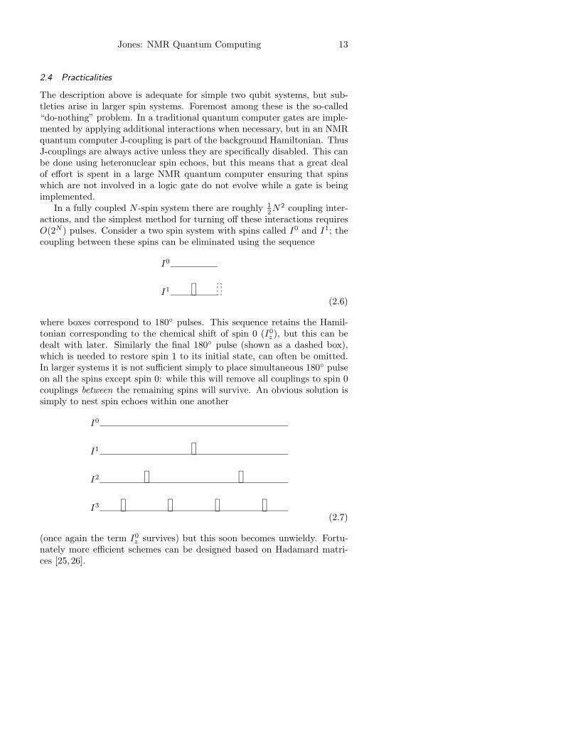
In a fully coupled N -spin system there are roughly 12N
2 coupling inter-actions, and the simplest method for turning off these interactions requiresO(2N ) pulses. Consider a two spin system with spins called I0 and I1; thecoupling between these spins can be eliminated using the sequence
I1
I0
(2.6)
where boxes correspond to 180 pulses. This sequence retains the Hamil-tonian corresponding to the chemical shift of spin 0 (I0
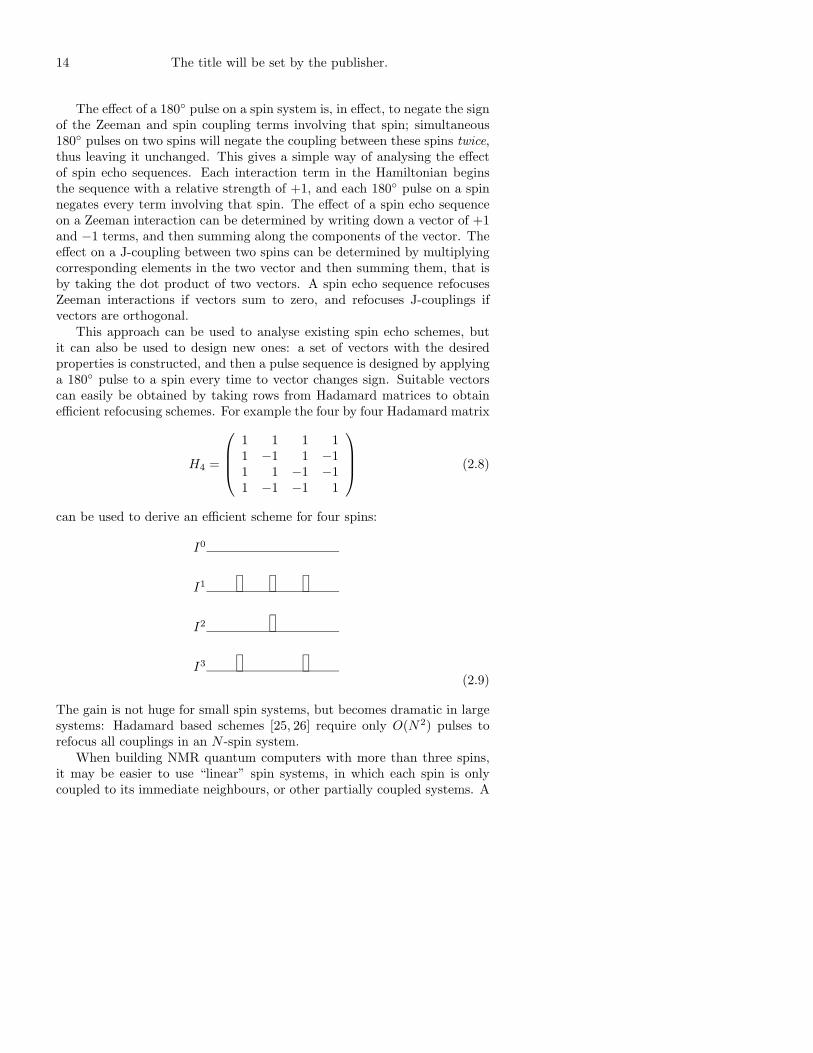
z ), but this can bedealt with later. Similarly the final 180 pulse (shown as a dashed box),which is needed to restore spin 1 to its initial state, can often be omitted.In larger systems it is not sufficient simply to place simultaneous 180 pulseon all the spins except spin 0: while this will remove all couplings to spin 0couplings between the remaining spins will survive. An obvious solution issimply to nest spin echoes within one another
I3
I2
I1
I0
(2.7)
(once again the term I0z survives) but this soon becomes unwieldy. Fortu-
nately more efficient schemes can be designed based on Hadamard matri-ces [25,26].
14 The title will be set by the publisher.
The effect of a 180 pulse on a spin system is, in effect, to negate the signof the Zeeman and spin coupling terms involving that spin; simultaneous180 pulses on two spins will negate the coupling between these spins twice,thus leaving it unchanged. This gives a simple way of analysing the effectof spin echo sequences. Each interaction term in the Hamiltonian beginsthe sequence with a relative strength of +1, and each 180 pulse on a spinnegates every term involving that spin. The effect of a spin echo sequenceon a Zeeman interaction can be determined by writing down a vector of +1and −1 terms, and then summing along the components of the vector. Theeffect on a J-coupling between two spins can be determined by multiplyingcorresponding elements in the two vector and then summing them, that isby taking the dot product of two vectors. A spin echo sequence refocusesZeeman interactions if vectors sum to zero, and refocuses J-couplings ifvectors are orthogonal.
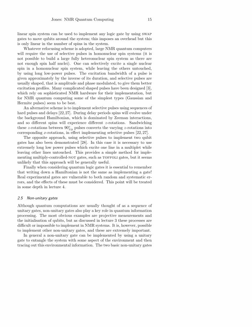
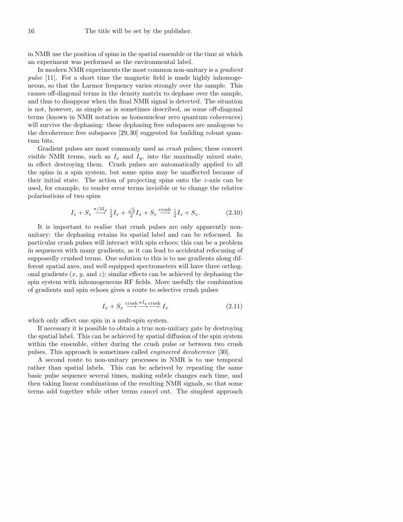
This approach can be used to analyse existing spin echo schemes, butit can also be used to design new ones: a set of vectors with the desiredproperties is constructed, and then a pulse sequence is designed by applyinga 180 pulse to a spin every time to vector changes sign. Suitable vectorscan easily be obtained by taking rows from Hadamard matrices to obtainefficient refocusing schemes. For example the four by four Hadamard matrix
H4 =
1 1 1 11 −1 1 −11 1 −1 −11 −1 −1 1
(2.8)
can be used to derive an efficient scheme for four spins:
I3
I2
I1
I0
(2.9)
The gain is not huge for small spin systems, but becomes dramatic in largesystems: Hadamard based schemes [25, 26] require only O(N2) pulses torefocus all couplings in an N -spin system.
When building NMR quantum computers with more than three spins,it may be easier to use “linear” spin systems, in which each spin is onlycoupled to its immediate neighbours, or other partially coupled systems. A
Jones: NMR Quantum Computing 15
linear spin system can be used to implement any logic gate by using swap
gates to move qubits around the system; this imposes an overhead but thisis only linear in the number of spins in the system.
Whatever refocusing scheme is adopted, large NMR quantum computerswill require the use of selective pulses in homonuclear spin systems (it isnot possible to build a large fully heteronuclear spin system as there arenot enough spin half nuclei). One can selectively excite a single nuclearspin in a homonuclear spin system, while leaving the others untouched,by using long low-power pulses. The excitation bandwidth of a pulse isgiven approximately by the inverse of its duration, and selective pulses areusually shaped, that is amplitude and phase modulated, to give them betterexcitation profiles. Many complicated shaped pulses have been designed [3],which rely on sophisticated NMR hardware for their implementation, butfor NMR quantum computing some of the simplest types (Gaussian andHermite pulses) seem to be best.
An alternative scheme is to implement selective pulses using sequences ofhard pulses and delays [22,27]. During delay periods spins will evolve underthe background Hamiltonian, which is dominated by Zeeman interactions,and so different spins will experience different z-rotations. Sandwichingthese z-rotations between 90±y pulses converts the varying z-rotations intocorresponding x-rotations, in effect implementing selective pulses [22,27].
The opposite approach, using selective pulses to implement two qubitgates has also been demonstrated [28]. In this case it is necessary to useextremely long low power pulses which excite one line in a multiplet whileleaving other lines untouched. This provides a simple method for imple-menting multiply-controlled-not gates, such as toffoli gates, but it seemsunlikely that this approach will be generally useful.
Finally when considering quantum logic gates it is essential to rememberthat writing down a Hamiltonian is not the same as implementing a gate!Real experimental gates are vulnerable to both random and systematic er-rors, and the effects of these must be considered. This point will be treatedin some depth in lecture 4.
2.5 Non-unitary gates
Although quantum computations are usually thought of as a sequence ofunitary gates, non-unitary gates also play a key role in quantum informationprocessing. The most obvious examples are projective measurements andthe initialisation of qubits, but as discussed in lecture 3 these processes aredifficult or impossible to implement in NMR systems. It is, however, possibleto implement other non-unitary gates, and these are extremely important.
In general a non-unitary gate can be implemented by using a unitarygate to entangle the system with some aspect of the environment and thentracing out this environmental information. The two basic non-unitary gates
16 The title will be set by the publisher.
in NMR use the position of spins in the spatial ensemble or the time at whichan experiment was performed as the environmental label.
In modern NMR experiments the most common non-unitary is a gradient
pulse [11]. For a short time the magnetic field is made highly inhomoge-neous, so that the Larmor frequency varies strongly over the sample. Thiscauses off-diagonal terms in the density matrix to dephase over the sample,and thus to disappear when the final NMR signal is detected. The situationis not, however, as simple as is sometimes described, as some off-diagonalterms (known in NMR notation as homonuclear zero quantum coherences)will survive the dephasing: these dephasing free subspaces are analogous tothe decoherence free subspaces [29, 30] suggested for building robust quan-tum bits.
Gradient pulses are most commonly used as crush pulses; these convertvisible NMR terms, such as Ix and Iy, into the maximally mixed state,in effect destroying them. Crush pulses are automatically applied to allthe spins in a spin system, but some spins may be unaffected because oftheir initial state. The action of projecting spins onto the z-axis can beused, for example, to render error terms invisible or to change the relativepolarisations of two spins
Iz + Szπ/3Iy
−→ 12Iz +
√3
2 Ix + Szcrush−→ 1
2Iz + Sz. (2.10)
It is important to realise that crush pulses are only apparently non-unitary: the dephasing retains its spatial label and can be refocused. Inparticular crush pulses will interact with spin echoes; this can be a problemin sequences with many gradients, as it can lead to accidental refocusing ofsupposedly crushed terms. One solution to this is to use gradients along dif-ferent spatial axes, and well equipped spectrometers will have three orthog-onal gradients (x, y, and z); similar effects can be achieved by dephasing thespin system with inhomogeneous RF fields. More usefully the combinationof gradients and spin echoes gives a route to selective crush pulses
Ix + Sxcrush−→
πIy
−→crush−→ Ix (2.11)
which only affect one spin in a mult-spin system.If necessary it is possible to obtain a true non-unitary gate by destroying
the spatial label. This can be achieved by spatial diffusion of the spin systemwithin the ensemble, either during the crush pulse or between two crushpulses. This approach is sometimes called engineered decoherence [30].
A second route to non-unitary processes in NMR is to use temporalrather than spatial labels. This can be acheived by repeating the samebasic pulse sequence several times, making subtle changes each time, andthen taking linear combinations of the resulting NMR signals, so that someterms add together while other terms cancel out. The simplest approach
Jones: NMR Quantum Computing 17
is to alter the relative phase of pulses, in which case it is known as phasecycling [11]. Phase cycling techniques were very widely used in conventionalNMR experiments, but in recent years have been largely superseded bygradients. They have, however, found new applications in NMR quantumcomputing where they form the basis of the popular temporal averaging
schemes for initialisation.
3 NMR quantum computers
In this section I will describe how NMR quantum computers overcome thedifficulties inherent in NMR to perform initialisation and readout. In par-ticular I will describe the use of pseudo-pure states, and the implicationsof this approach for the efficiency of NMR quantum computing. Finally Iwill briefly describe the implementation of a quantum cloning on an NMRquantum computer.
3.1 Introduction
From the description given in the previous lecture it would seem that NMRwas very well suited to the task of implementing quantum computers. Thereare, however, substantial problems with NMR as a quantum informationprocessing technology [31], which stem from difficulties in initialising nuclearspin states and in reading out the final result.
Conventional designs for quantum computers [32] use single quantumsystems which start in a well defined initial state. While details may vary,this initialisation is usually achieved by cooling the system to its thermo-dynamic ground state. NMR quantum computers [19–22], by contrast, usean ensemble of molecules which start in a hot thermal state, because evenfor the very large fields used in NMR spectrometers the Zeeman energy gapbetween the two spin states is tiny compared to kT . One could imaginelowering the temperature so that NMR enters the low temperature regime,but this would require cooling the system well below 1 mK; although thisis possible the sample would certainly not remain in the liquid state. Apotentially better approach is to use non-Boltzmann initial populations,as discussed in lecture 5. Almost all implementation of NMR quantumcomputing, however, simply sidestep this issue by forming a “pseudo-pure”initial state from the thermal state as discussed below.
Similar problems also occur with methods for reading out the final re-sult. Conventional quantum computers achieve read out by hard (projec-tive) measurements, while NMR quantum computers use weak ensemblemeasurements, which do not project the spin system. This can be seen byrealising that a conventional NMR measurement (observation of the freeinduction decay) can be described quantum mechanically as the continuousand simultaneous observation of two non-commuting observables, Ix and Iy.
18 The title will be set by the publisher.
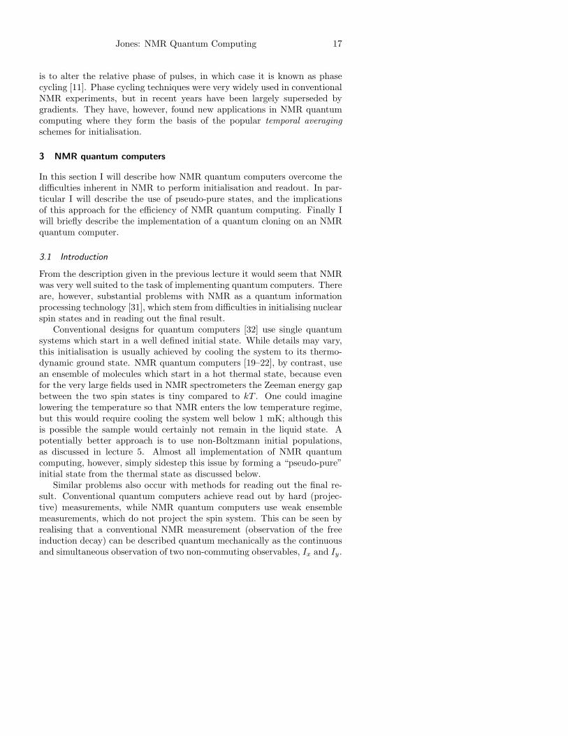
This is also the approach used for readout in NMR quantum computers, anda simple example is shown in Fig. 1
Fig. 1. NMR spectrum showing readout from a two qubit NMR quantum com-
puter based on the two 1H nuclei in cytosine [33]; the negative intensity on the
left hand multiplet indicates that the corresponding qubit was in state |1〉, while
the positive intensity indicates that this qubit was in state |0〉.
These weak measurements might seem more powerful than conventionalprojective measurements, but in fact they are less useful for two reasons.Firstly the use of projective measurements permits the use of measurementsfollowed by classical control; by contrast NMR quantum computers can onlyuse quantum control methods. More importantly, projective measurementsprovide an excellent initialisation method: just measure a bit, and then flipit if it has the wrong value! In particular reinitialisation of ancilla qubitsthrough the use of projective measurements plays a key role in quantumerror-correction protocols [34].
3.2 Pseudo-pure states
The history of NMR quantum computing in effect begins with the realisationby David Cory and coworkers [19,20] that while it is difficult to form a pureinitial state it is easy to form states whose behavior is almost identical. Suchstates, known a pseudo-pure states or effective pure states, take the form
ρ = (1 − ε)1
2n+ ε|0〉〈0|, (3.1)
that is mixtures of the maximally mixed state and the desired initial statewith purity ε. As the maximally mixed state does not evolve under anyunitary transformation it will be unchanged by any quantum computation.Furthermore, all NMR observables are traceless [11], and so the maximallymixed state gives no observable signal. For this reason the presence of themaximally mixed state can, in effect, be ignored, and the behaviour of apseudo-pure state is identical to that of the corresponding pure state up toa scaling factor [22].
As an example, consider a homonuclear spin system of two spin-halfnuclei. This has four energy levels with nearly equal populations, but thepopulation of the lowest level will of course be slightly greater than that ofany other level. This excess population provides the basis of pseudo-pure
Jones: NMR Quantum Computing 19
state formation, but the state as described is not a pseudo-pure state, asthe upper levels do not all have the same population. Suppose, however,that some non-unitary process is applied which equalises the populations ofthe upper levels, while leaving the lowest level untouched: the result willbe the desired pseudo-pure state [35]. To understand the behaviour of thisstate imagine going through the ensemble, taking out molecules in groupsof four (one in each spin state) and placing them in a box; eventually therewill be a large box containing equal populations of all four spin states anda small excess of the |00〉 spin state remaining. The NMR signals from themolecules in the box will all cancel out, leaving only the signal from thesmall excess: the pseudo-pure state.
Pseudo-pure states can also be described more accurately using theproduct operator approach [22, 36]. The Boltzmann equilibrium state ofa homonuclear two-spin system is approximately
ρB ≈ 12E + δ(Iz + Sz) = 1
2E + δ1, 0, 0,−1 (3.2)
where the braces indicate a diagonal density matrix described by listing itsdiagonal elements. The ideal pure ground state takes the form
ρ0 = 12 ( 1
2E + Iz + Sz + 2IzSz) = 1, 0, 0, 0 (3.3)
and so forming a pseudo-pure ground state will require the creation of a2IzSz component and the rescaling of other terms so that each term ispresent in the correct relative quantity. Clearly this will require a combina-tion of unitary and non-unitary processes, and three main approaches havebeen described.
The original spatial avaeraging method of Cory et al. [19,20] for creatinga pseudo-pure state in a two spin system used a sequence of (unitary) pulsesand delays combined with (non-unitary) crush gradients. The method iseasily understood using product operators:
Iz + Sz60Sx−→ Iz + 1
2Sz −√
32 Sy
crush−→ Iz + 1
2Sz45Ix−→ 1√
2Iz −
1√2Iy + 1
2Sz
Ising−→ 1√
2Iz + 1√
22IxSz + 1
2Sz
45Ix−→ 12Iz −
12Ix + 1
22IxSz + 12Sz + 1
22IzSzcrush−→ 1
2 (Iz + Sz + 2IzSz). (3.4)
An widely used alternative, temporal averaging [37], uses permutationoperations to create different initial states
Iz + SzP0−→ 1, 0, 0,−1
20 The title will be set by the publisher.
Iz + SzP1−→ 1, 0,−1, 0
Iz + SzP2−→ 1,−1, 0, 0 (3.5)
and averaging over these three separate experiments gives an effective purestate
ρTA = 1,− 13 ,−
13 ,−
13. (3.6)
This method has the advantage of being easy to understand and to gen-eralise to larger spin system, but the disadvantage that several differentexperiments are required. Indeed if the most obvious scheme, exhaustivepermutation, is implemented a very large number of experiments may be re-quired; fortunately less profligate partial averaging schemes are known [37].
Finally the logical labelling approach of Gershenfeld and Chuang [21]provides a conceptually elegant method for using naturally occurring subsetsof levels in larger systems as pseudo-pure states. As an example consider athree spin system
Iz + Sz +Rz = 123, 1, 1,−1, 1,−1,−1,−3 (3.7)
and pick out the subset of four levels with relative populations 3, −1, −1and −1, that is the levels |000〉, |011〉, |101〉 and |110〉. The most directapproach is just to work in this subset, but it usually more convenient topermute populations so that the levels |000〉, |001〉, |010〉 and |011〉 can beused; this makes implementing logic gates much simpler.
Perhaps the most practical general scheme for preparing pseudo-purestates is based on the use of “cat” states [24], which are states of the form
ψn± = |00 . . . 0〉 ± |11 . . . 1〉 (3.8)
for an n-qubit system, that is equally weighted superpositions of the statein which all n qubits are in |0〉 and the state in which all qubits are in |1〉. Itis easy both to reach the state ψn+ starting from the ground state |00 . . . 0〉,and to convert the cat state back to the ground state. This may not seemuseful, but it is relatively simple to design non-unitary filter schemes, usingeither spatial or temporal averaging, which convert all states except ψn± intothe maximally mixed state. The Boltzmann equilibrium state can thus beconverted to a mixed state including a component of ψn±, and after filtrationthe ψn+ state can be converted back to |00 . . . 0〉. The filter schemes, however,also retain any ψn− component, and this is converted into |10 . . . 0〉. Theoverall effect is to produce the state Iz ⊗ |0 . . . 0〉〈0 . . . 0|, that is a pseudo-pure state of n− 1 qubits.
3.3 Efficiency of NMR quantum computing
The discussion so far has neglected any consideration of the level of puritywhich can be achieved in a pseudo-pure state; this is most simply quantified
Jones: NMR Quantum Computing 21
by the value of ε in Eq. 3.1. At one level this is unimportant, as ε simplydetermines the intensity of the observed NMR signal, but if ε becomes toosmall this will render the NMR signal undetectable. Unfortunately for NMRquantum computing, the value of ε drops exponentially with the number ofqubits in the system: for every additional qubit the available signal intensityapproximately halves [38].
This effect is not, as is sometimes suggested, a peculiar fault of NMRquantum computers: rather it is a simple consequence of working in the hightemperature limit. It does, however, mean that pseudo-pure states extractedfrom thermal equilibrium systems cannot provide a route to scalable NMRquantum computers.
More controversially some authors have implied that NMR quantumcomputers are not quantum computers at all! How this claim is assesseddepends on exactly what is meant by “NMR quantum computers”, andeven what is meant by “quantum computing”. However, while there issubstantial room for philosophical debates, the underlying science is nowrelatively clear. On the one hand it is known that high temperature pseudo-pure states cannot lead to provably entangled states [39], and that suchsystems cannot give efficient implementations of Shor’s quantum factoringalgorithm [40]. On the other hand it so far proved impossible to developa purely classical model of pseudo-pure state NMR quantum computing:while it is possible to describe the state of an NMR device at any point in acomputation using a classical model, it appears to be impossible to developa classical model of the transitions between these states [41].
It is also vital to remember that these arguments apply only to NMRquantum computers built using pseudo-pure states, and that there are othertypes of NMR quantum computing. For example some quantum algorithmsonly require one pure qubit: the other qubits can be in maximally mixedstates [42]. Indeed, even the single “pure” qubit need not be pure: a pseudo-pure state will suffice. This type of NMR quantum computing is clearlyscalable, although it can only be used for a limited range of algorithms. Analternative approach is to use a scheme described by Schulman and Vazirani,which allows a small number of nearly pure qubits to be distilled from alarge number of impure qubits using only unitary operations [43]. Thisscheme needs O(ε−2) impure spins for each pure spin extracted: this is aconstant multiplicative overhead, and so has no scaling problem. Thus hightemperature states, such as those used in NMR, do allow true quantumcomputing! Unfortunately the overhead for NMR systems of about 1010
means that this method has only theoretical interest.
3.4 NMR quantum cloning
Finally I will end this lecture by briefly describing an NMR implementa-tion of approximate quantum cloning [44]. This experiment is complicated
22 The title will be set by the publisher.
enough to be interesting, but simple enough that the basic ideas can bedescribed in a fairly straightforward manner.
The no-cloning theorem, which states that an unknown quantum statecannot be exactly copied [45], is one of the oldest results in quantum infor-mation theory. Approximate quantum cloning is, however, possible, and arange of different schemes have been described. If one qubit is convertedinto two identical copies, such that the fidelity of the copies is independentof the initial state, then the maximum fidelity that can be achieved is 5
6 ,and an explicit quantum circuit which achieves this is known [46]. If a state|ψ〉 is cloned, the two copies take the form
56 |ψ〉〈ψ| +
16 |ψ
⊥〉〈ψ⊥| = 23 |ψ〉〈ψ| +
13 (1/2). (3.9)
This circuit can also be used to clone a mixed state, ρ producing even moremixed clones of the form
23ρ+ 1
3 (1/2). (3.10)
In the language of vectors on Bloch spheres, the two clones have Blochvectors parallel to the original Bloch vector, but with only 2
3 the length [44].
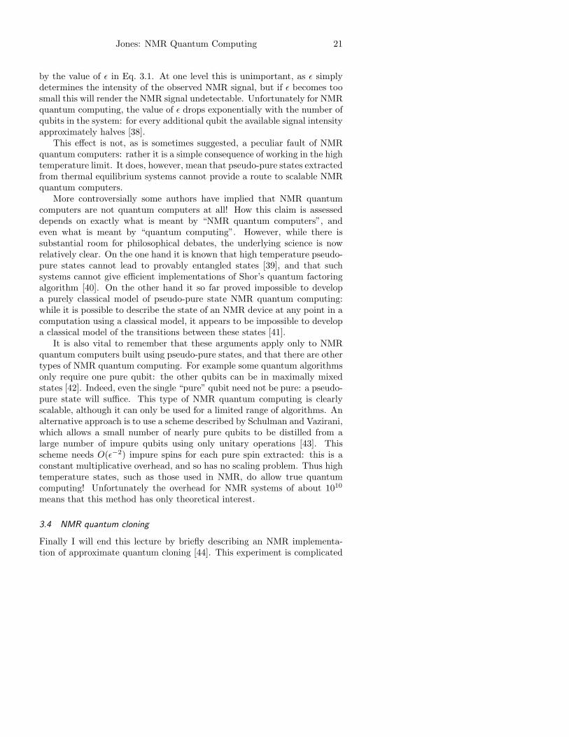
The cloning circuit comprises two stages: preparation, which preparestwo qubits into an initial “blank paper” state, suitable for receiving a copy,and copying, in which the initial qubit is copied onto these qubits. As thepreparation stage simply prepares two blank qubits, and is independent ofthe state of the unknown qubit, the preparation stage can be replaced byany other transformation which has the same effect, and the NMR imple-mentation, which is shown in Fig. 2 does indeed use a modified preparationstage. The copying stage, however, must implement the correct unitarytransformation, and the implementation used the conventional copying cir-cuit.
Fig. 2. A modified version of the approximate quantum cloning network: the new
version is simpler to implement on the NMR system used. Filled circles connected
by control lines indicate controlled phase shift gates, empty circles indicate single
qubit Hadamard gates, while grey circles indicate other single qubit rotations.
The two rotation angles in the preparation stage are θ1 = arcsin(
1/√
3)
≈ 35
and θ2 = π/12 = 15.
Jones: NMR Quantum Computing 23
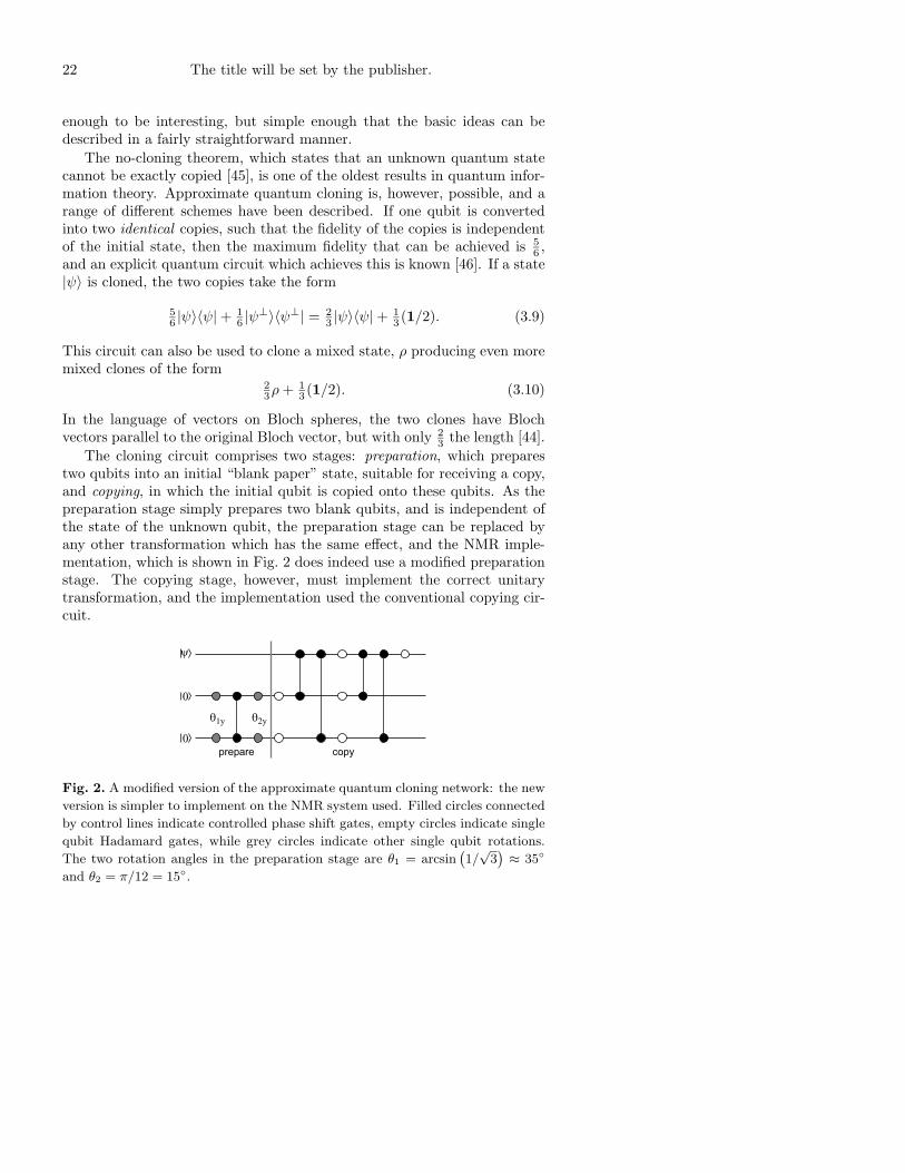
The cloning circuit was implemented on a three-qubit NMR quantumcomputer based on the molecule based on the single 31P nucleus (P ) andthe two 1H nuclei (A and B) in E-(2-chloroethenyl)phosphonic acid (Fig. 3)dissolved in D2O. The NMR pulse sequence used is shown in Fig. 4. This
100 50 0 -50 -100
Hz
C
C
P
Cl OD
O
OD
HA
HB
Fig. 3. The three qubit system provided by E-(2-chloroethenyl)phosphonic acid
dissolved in D2O and its 1H NMR spectrum. Following standard NMR conven-
tions the spectrum has been plotted with frequencies measured as offsets from
the reference RF frequency, and with frequency increasing from right to left. The
broad peak near −50 Hz can be ignored.
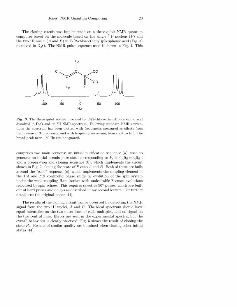
comprises two main sections: an initial purification sequence (a), used togenerate an initial pseudo-pure state corresponding to Pz ⊗ |0A0B〉〈0A0B |,and a preparation and cloning sequence (b), which implements the circuitshown in Fig. 2, cloning the state of P onto A and B. Both of these are builtaround the “echo” sequence (c), which implements the coupling element ofthe PA and PB controlled phase shifts by evolution of the spin systemunder the weak coupling Hamiltonian with undesirable Zeeman evolutionsrefocused by spin echoes. This requires selective 90 pulses, which are builtout of hard pulses and delays as described in my second lecture. For furtherdetails see the original paper [44].
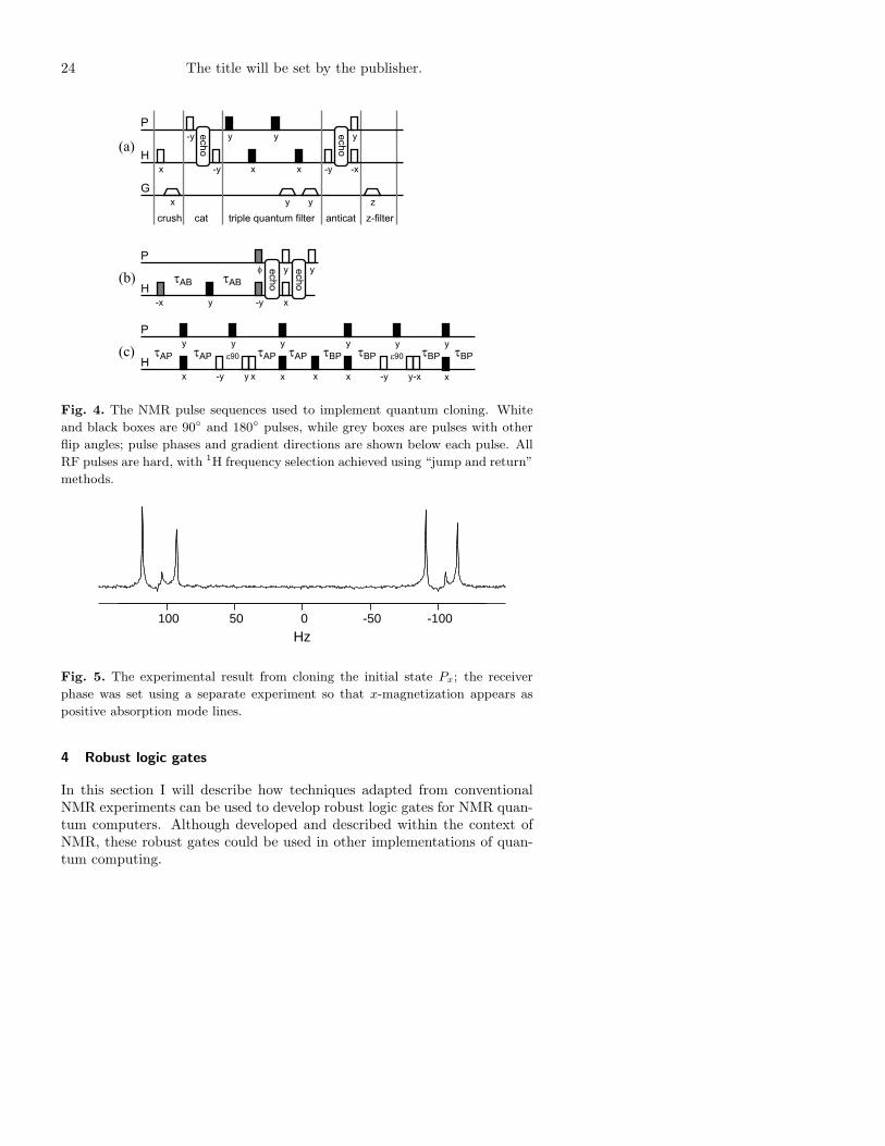
The results of the cloning circuit can be observed by detecting the NMRsignal from the two 1H nuclei, A and B. The ideal spectrum should haveequal intensities on the two outer lines of each multiplet, and no signal onthe two central lines. Errors are seen in the experimental spectra, but theoverall behaviour is clearly observed: Fig. 5 shows the result of cloning thestate Px. Results of similar quality are obtained when cloning other initialstates [44].
24 The title will be set by the publisher.
x
-y y y
-y x x -y
y
-x
x y y z
H
P
G
crush cat triple quantum filter anticat z-filter
y
f
-x -y
y y
x
H
P
tAB tAB
x -x
y yy yy y
x xx xx-y -yy y
H
P
tAP tAP tAPe90 e90tAP tBP tBP tBP tBP
(a)
(b)
(c)
echo
echo
echo
echo
Fig. 4. The NMR pulse sequences used to implement quantum cloning. White
and black boxes are 90 and 180 pulses, while grey boxes are pulses with other
flip angles; pulse phases and gradient directions are shown below each pulse. All
RF pulses are hard, with 1H frequency selection achieved using “jump and return”
methods.
100 50 0 -50 -100
Hz
Fig. 5. The experimental result from cloning the initial state Px; the receiver
phase was set using a separate experiment so that x-magnetization appears as
positive absorption mode lines.
4 Robust logic gates
In this section I will describe how techniques adapted from conventionalNMR experiments can be used to develop robust logic gates for NMR quan-tum computers. Although developed and described within the context ofNMR, these robust gates could be used in other implementations of quan-tum computing.
Jones: NMR Quantum Computing 25
4.1 Introduction
Quantum computers implement logic gates as periods of evolution underHamiltonians which can be external (e.g., RF pulses) or internal (e.g., Isingcouplings). Computation requires extremely accurate logic gates, and thusextremely accurate control of evolution rates. Naive estimates suggest thatit may be difficult or impossible to control Hamiltonians with sufficientaccuracy, but fortunately robust logic gates can be designed to toleratesmall errors in these rates.
The approach described here is based on the NMR concept of composite
rotations [3, 9, 47, 48], which have long been used to reduce the impact ofsystematic errors on conventional NMR experiments, but the basic ideais general and can be applied in many other fields. As usual it is notnecessary to design robust versions of every conceivable logic gate: it sufficesto develop a complete set of one and two qubit gates.
When considering the accuracy of logic gates it is necessary to measurethe fidelity of the actual operation V in comparison with the desired oper-ation U , and an obvious measure is provided by the propagator fidelity [49]
F =| tr (V U†)|
tr (UU†)(4.1)
where it is necessary to take the absolute value of the numerator to dealwith (irrelevant) differences in global phases. The propagator fidelity worksfor any unitary operation, although it can be over complicated in practiceand alternative measures have been suggested.
4.2 Composite rotations
The use of composite rotations to reduce the effects of systematic errors inconventional NMR experiments relies on the fact that any state of a singleisolated qubit can be mapped to a point on the Bloch sphere, and any uni-tary operation on a single isolated qubit corresponds to a rotation on theBloch sphere. The result of applying any series of rotations (a composite ro-tation) is itself a rotation, and so there are many apparently equivalent waysof performing a desired rotation. These different methods may, however,show different sensitivity to errors: composite rotations can be designed tobe much less error prone than simple rotations!
A rotation can go wrong in two basic ways: the rotation angle can bewrong or the rotation axis can be wrong. In an NMR experiment (viewedin the rotating frame) ideal RF pulses cause rotation of a spin throughan angle θ = ω1t around an axis in the xy-plane. So called pulse length
errors occur when the pulse power ω1 is incorrect, so that the flip angle θis systematically wrong by some fraction. This can be due to experimentercarelessness, but more usually arises from the inhomogeneity in the RF field
26 The title will be set by the publisher.
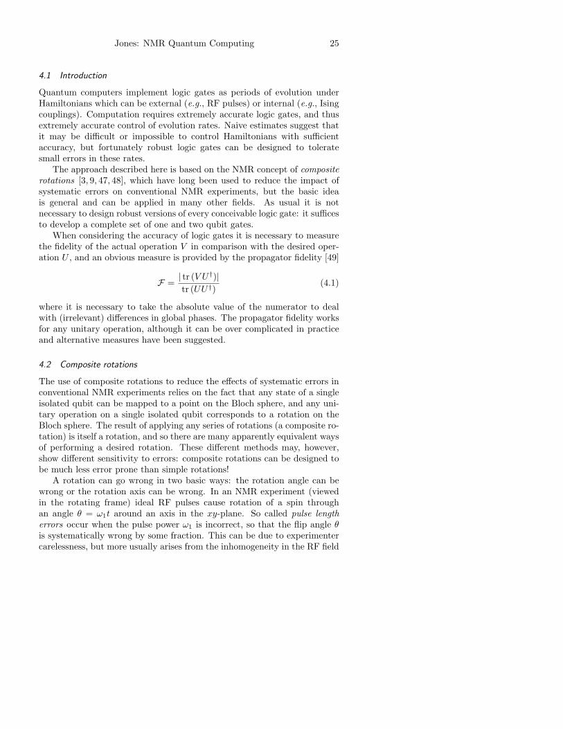
over a macroscopic sample. The second type of error, off-resonance effects
(Fig. 6), occur when the excitation frequency doesnt match the transition
Fig. 6. Effect of applying an off-resonance 180 pulse to a spin with initial state
Iz; the spin rotates around a tilted axis. Trajectories are shown for small, medium
and large off-resonance effects.
frequency, so that the Hamiltonian is the sum of RF and off-resonance terms.This results in rotations around a tilted axis, and the rotation angle is alsoincreased.
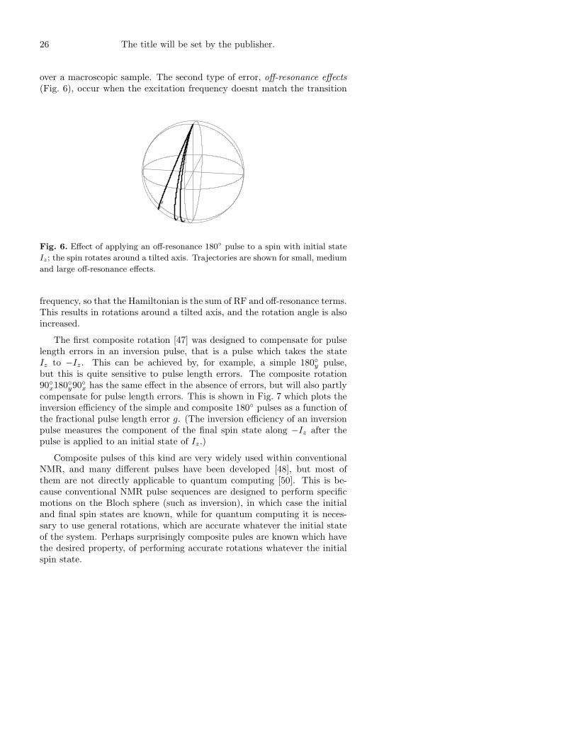
The first composite rotation [47] was designed to compensate for pulselength errors in an inversion pulse, that is a pulse which takes the stateIz to −Iz. This can be achieved by, for example, a simple 180y pulse,but this is quite sensitive to pulse length errors. The composite rotation90x180y90x has the same effect in the absence of errors, but will also partlycompensate for pulse length errors. This is shown in Fig. 7 which plots theinversion efficiency of the simple and composite 180 pulses as a function ofthe fractional pulse length error g. (The inversion efficiency of an inversionpulse measures the component of the final spin state along −Iz after thepulse is applied to an initial state of Iz.)
Composite pulses of this kind are very widely used within conventionalNMR, and many different pulses have been developed [48], but most ofthem are not directly applicable to quantum computing [50]. This is be-cause conventional NMR pulse sequences are designed to perform specificmotions on the Bloch sphere (such as inversion), in which case the initialand final spin states are known, while for quantum computing it is neces-sary to use general rotations, which are accurate whatever the initial stateof the system. Perhaps surprisingly composite pules are known which havethe desired property, of performing accurate rotations whatever the initialspin state.
Jones: NMR Quantum Computing 27
-1 -0.5 0 0.5 1g
-1
-0.5
0
0.5
1
inve
rsio
n ef
fici
ency
Fig. 7. The inversion efficiency of a simple 180 pulse (dashed line) and of the
composite pulse 90
x180
y90
x (solid line) as a function of the fractional pulse length
error g. The way in which the composite pulse works can be understood by
examining trajectories on the Bloch sphere, which are shown on the right for
three values of g.
4.3 Quaternions and single qubit gates
Quaternions provide a simple and powerful way of describing rotations (sin-gle qubit gates), as they can be easily formed, combined, and compared. Thequaternion corresponding to a θ rotation around an axis at an azimuthalangle φ in the xy-plane is given by
qθφ = s,v = cos(θ/2), sin(θ/2)(cos(φ), sin(φ), 0) (4.2)
where s is a scalar depending on the rotation angle, and v is a vector whoselength depends on the rotation angle and which lies parallel to the rotationaxis. The result of applying two rotations is given by the quaternion product
q1 ∗ q2 = s1 · s2 − v1 · v2, s1v2 + s2v1 + v1 ∧ v2 (4.3)
and two quaternions can be compared using the quaternion fidelity
F(q1, q2) = |q1 · q2| = |s1 · s2 + v1 · v2|. (4.4)
As a simple example consider a not gate, that is a 180x rotation. Thequaternion for an ideal rotation is
q0 = 0, (1, 0, 0) (4.5)
while the quaternion representing this rotation in the presence of a fractionalpulse length error g is
q1 = cos[(1 + g)π/2], (sin[(1 + g)π/2], 0, 0) (4.6)
28 The title will be set by the publisher.
and so the quaternion fidelity is
F1 = | sin((1 + g)π/2)| = | cos(gπ/2)| ≈ 1 −π2g2
8(4.7)
As an alternative consider the conventional composite pulse sequence for a180x rotation, 90y180x90y, which has the quaternion form
q2 = sin2[gπ/2], (cos[gπ/2],− sin[gπ]/2, 0) (4.8)
and gives exactly the same fidelity, F2 = | cos(gπ/2)| = F1. This confirmsthat the conventional sequence does not actually correct for errors whenconsidered as a general rotation: the good behaviour for certain initial statesis obtained at the cost of poor behaviour for other initial states.
An example of a not gate which does give genuine improvement [51,52]is provided by the sequence 900180φ3603φ180φ900, with φ = arccos(−1/4).The quaternion for this composite rotation in the presence of errors is com-plicated, but its fidelity is given by
F3 ≈ 1 −5π6g6
1024(4.9)
showing that the second and fourth order error terms are completely can-celled. This BB1 sequence was originally developed by Wimperis for con-ventional NMR experiments [51], and later rederived using quaternions inthe context of NMR quantum computing [52]. As shown in Fig. 8 the BB1gate outperforms a naive not gate for all pulse length errors g, especiallyfor errors in the range ±25%. Its behaviour is essentially perfect for errorsof less than 1%.
Similar gates can be developed to tackle off-resonance effects. Intrigu-ingly the sequence 90x180y90x provides some compensation for off-resonanceeffects as long as the pulse length is correct, but as before this compensa-tion only occurs for inversion, and so the composite pulse is not suitable forquantum computing. However suitable composite rotations are known: anearly result by Tycko [53] has been refined and extended [52, 54]: a simpleθx rotation should be replaced by the corpse sequence of three rotationsalong x, −x and x with
θ1 = 2π +θ
2− arcsin
(
sin(θ/2)
2
)
θ2 = 2π − 2 arcsin
(
sin(θ/2)
2
)
θ3 =θ
2− arcsin
(
sin(θ/2)
2
)
. (4.10)
The simultaneous correction of pulse length errors and off-resonance effectsis still being studied [52].
Jones: NMR Quantum Computing 29
0.001 0.01 0.1 110
-18
10-16
10-14
10-12
10-10
10-8
10-6
10-4
10-2
100
g
infi
deli
ty
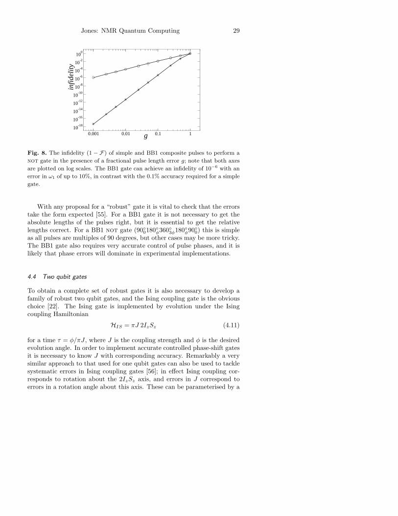
Fig. 8. The infidelity (1 − F) of simple and BB1 composite pulses to perform a
not gate in the presence of a fractional pulse length error g; note that both axes
are plotted on log scales. The BB1 gate can achieve an infidelity of 10−6 with an
error in ω1 of up to 10%, in contrast with the 0.1% accuracy required for a simple
gate.
With any proposal for a “robust” gate it is vital to check that the errorstake the form expected [55]. For a BB1 gate it is not necessary to get theabsolute lengths of the pulses right, but it is essential to get the relativelengths correct. For a BB1 not gate (900180φ3603φ180φ900) this is simpleas all pulses are multiples of 90 degrees, but other cases may be more tricky.The BB1 gate also requires very accurate control of pulse phases, and it islikely that phase errors will dominate in experimental implementations.
4.4 Two qubit gates
To obtain a complete set of robust gates it is also necessary to develop afamily of robust two qubit gates, and the Ising coupling gate is the obviouschoice [22]. The Ising gate is implemented by evolution under the Isingcoupling Hamiltonian
HIS = πJ 2IzSz (4.11)
for a time τ = φ/πJ , where J is the coupling strength and φ is the desiredevolution angle. In order to implement accurate controlled phase-shift gatesit is necessary to know J with corresponding accuracy. Remarkably a verysimilar approach to that used for one qubit gates can also be used to tacklesystematic errors in Ising coupling gates [56]; in effect Ising coupling cor-responds to rotation about the 2IzSz axis, and errors in J correspond toerrors in a rotation angle about this axis. These can be parameterised by a
30 The title will be set by the publisher.
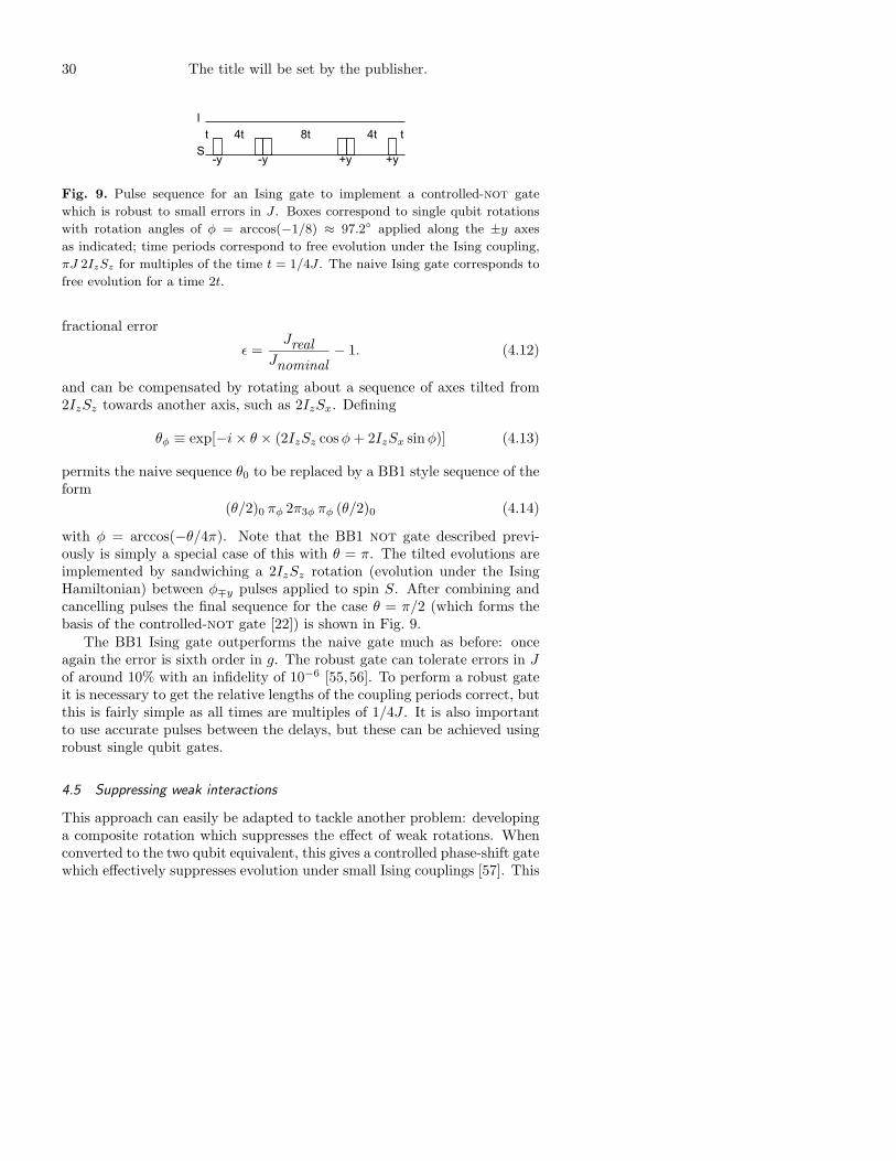
Fig. 9. Pulse sequence for an Ising gate to implement a controlled-not gate
which is robust to small errors in J . Boxes correspond to single qubit rotations
with rotation angles of φ = arccos(−1/8) ≈ 97.2 applied along the ±y axes
as indicated; time periods correspond to free evolution under the Ising coupling,
πJ 2IzSz for multiples of the time t = 1/4J . The naive Ising gate corresponds to
free evolution for a time 2t.
fractional error
ε =Jreal
Jnominal− 1. (4.12)
and can be compensated by rotating about a sequence of axes tilted from2IzSz towards another axis, such as 2IzSx. Defining
θφ ≡ exp[−i× θ × (2IzSz cosφ+ 2IzSx sinφ)] (4.13)
permits the naive sequence θ0 to be replaced by a BB1 style sequence of theform
(θ/2)0 πφ 2π3φ πφ (θ/2)0 (4.14)
with φ = arccos(−θ/4π). Note that the BB1 not gate described previ-ously is simply a special case of this with θ = π. The tilted evolutions areimplemented by sandwiching a 2IzSz rotation (evolution under the IsingHamiltonian) between φ∓y pulses applied to spin S. After combining andcancelling pulses the final sequence for the case θ = π/2 (which forms thebasis of the controlled-not gate [22]) is shown in Fig. 9.
The BB1 Ising gate outperforms the naive gate much as before: onceagain the error is sixth order in g. The robust gate can tolerate errors in Jof around 10% with an infidelity of 10−6 [55,56]. To perform a robust gateit is necessary to get the relative lengths of the coupling periods correct, butthis is fairly simple as all times are multiples of 1/4J . It is also importantto use accurate pulses between the delays, but these can be achieved usingrobust single qubit gates.
4.5 Suppressing weak interactions
This approach can easily be adapted to tackle another problem: developinga composite rotation which suppresses the effect of weak rotations. Whenconverted to the two qubit equivalent, this gives a controlled phase-shift gatewhich effectively suppresses evolution under small Ising couplings [57]. This
Jones: NMR Quantum Computing 31
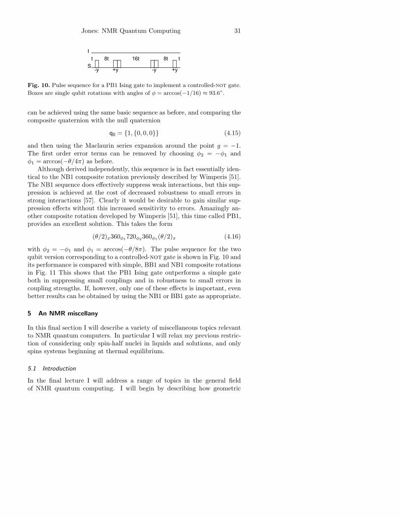
Fig. 10. Pulse sequence for a PB1 Ising gate to implement a controlled-not gate.
Boxes are single qubit rotations with angles of φ = arccos(−1/16) ≈ 93.6.
can be achieved using the same basic sequence as before, and comparing thecomposite quaternion with the null quaternion
q0 = 1, 0, 0, 0 (4.15)
and then using the Maclaurin series expansion around the point g = −1.The first order error terms can be removed by choosing φ2 = −φ1 andφ1 = arccos(−θ/4π) as before.
Although derived independently, this sequence is in fact essentially iden-tical to the NB1 composite rotation previously described by Wimperis [51].The NB1 sequence does effectively suppress weak interactions, but this sup-pression is achieved at the cost of decreased robustness to small errors instrong interactions [57]. Clearly it would be desirable to gain similar sup-pression effects without this increased sensitivity to errors. Amazingly an-other composite rotation developed by Wimperis [51], this time called PB1,provides an excellent solution. This takes the form
(θ/2)x360φ1720φ2
360φ1(θ/2)x (4.16)
with φ2 = −φ1 and φ1 = arccos(−θ/8π). The pulse sequence for the twoqubit version corresponding to a controlled-not gate is shown in Fig. 10 andits performance is compared with simple, BB1 and NB1 composite rotationsin Fig. 11 This shows that the PB1 Ising gate outperforms a simple gateboth in suppressing small couplings and in robustness to small errors incoupling strengths. If, however, only one of these effects is important, evenbetter results can be obtained by using the NB1 or BB1 gate as appropriate.
5 An NMR miscellany
In this final section I will describe a variety of miscellaneous topics relevantto NMR quantum computers. In particular I will relax my previous restric-tion of considering only spin-half nuclei in liquids and solutions, and onlyspins systems beginning at thermal equilibrium.
5.1 Introduction
In the final lecture I will address a range of topics in the general fieldof NMR quantum computing. I will begin by describing how geometric
32 The title will be set by the publisher.
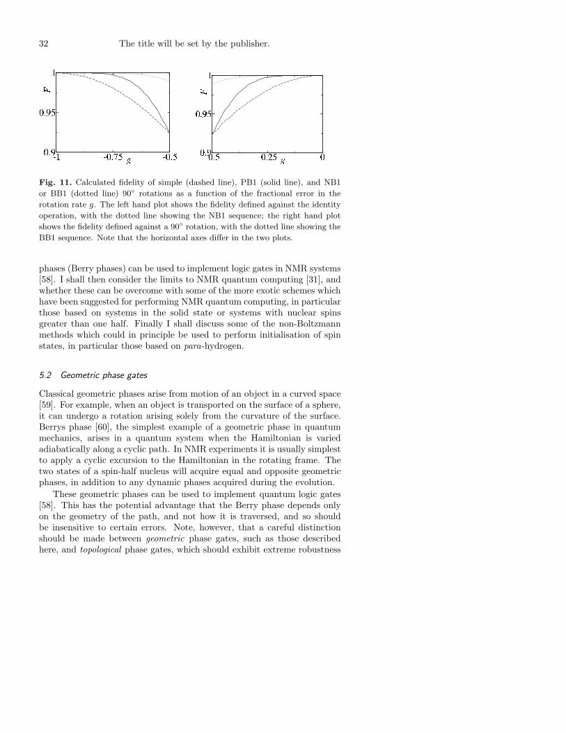
Fig. 11. Calculated fidelity of simple (dashed line), PB1 (solid line), and NB1
or BB1 (dotted line) 90 rotations as a function of the fractional error in the
rotation rate g. The left hand plot shows the fidelity defined against the identity
operation, with the dotted line showing the NB1 sequence; the right hand plot
shows the fidelity defined against a 90 rotation, with the dotted line showing the
BB1 sequence. Note that the horizontal axes differ in the two plots.
phases (Berry phases) can be used to implement logic gates in NMR systems[58]. I shall then consider the limits to NMR quantum computing [31], andwhether these can be overcome with some of the more exotic schemes whichhave been suggested for performing NMR quantum computing, in particularthose based on systems in the solid state or systems with nuclear spinsgreater than one half. Finally I shall discuss some of the non-Boltzmannmethods which could in principle be used to perform initialisation of spinstates, in particular those based on para-hydrogen.
5.2 Geometric phase gates
Classical geometric phases arise from motion of an object in a curved space[59]. For example, when an object is transported on the surface of a sphere,it can undergo a rotation arising solely from the curvature of the surface.Berrys phase [60], the simplest example of a geometric phase in quantummechanics, arises in a quantum system when the Hamiltonian is variedadiabatically along a cyclic path. In NMR experiments it is usually simplestto apply a cyclic excursion to the Hamiltonian in the rotating frame. Thetwo states of a spin-half nucleus will acquire equal and opposite geometricphases, in addition to any dynamic phases acquired during the evolution.
These geometric phases can be used to implement quantum logic gates[58]. This has the potential advantage that the Berry phase depends onlyon the geometry of the path, and not how it is traversed, and so shouldbe insensitive to certain errors. Note, however, that a careful distinctionshould be made between geometric phase gates, such as those describedhere, and topological phase gates, which should exhibit extreme robustness
Jones: NMR Quantum Computing 33
[61]. Topological phase gates are an exciting idea, but have not yet beendemonstrated experimentally.
To see how geometric phases can be implemented in NMR, recall thatoff-resonance excitation gives rise to a Hamiltonian which is tilted in therotating frame. The tilt angle can be controlled by varying the off-resonancefraction, which can be achieved either by changing the frequency offset orby changing the RF intensity. The phase angle can be controlled by simplychanging the phase of the RF. Thus the Hamiltonian can be moved aroundthe Bloch sphere at will. The simplest scheme is to begin by raising the RFintensity slowly from 0 up to some maximum value, so that the Hamiltonianis tilted away from the z-axis to some final tilt angle θ, changing the phaseof the RF so that the Hamiltonian rotates around a cone with cone angle θ,and finally reducing the RF intensity back to zero. The geometric phasespicked up during this process are
±γ = ±Ω/2 = ±π(1 − cos θ) (5.1)
where the ± sign corresponds to the phase picked up by the ± 12 spin states,
which correspond to qubits in states |0〉 and |1〉.The geometric phase is most conveniently observed in NMR experiments
by applying the adiabatic sweep to a spin in a superposition state, suchas Ix; the phases are then seen as a shift 2γ in the relative phase of thesuperposition, that is as a 2γIz rotation. However if the experiment iscarried out as described the desired geometric phase will be completelyswamped by the dynamic phase which arises simply from the integratedsize of the Hamiltonian. Even worse, this dynamic phase will vary overthe sample, as a result of RF inhomogeneity, and so when the final signalis averaged over the macroscopic ensemble the dynamic phase will causeextensive dephasing. It is, therefore, essential to refocus the dynamic phase,and as usual this can be achieved by using spin echoes: two adiabatic sweepsare applied with the second sweep sandwiched between a pair of 180 pulses.It might seem that the geometric phase would also be refocussed by thisapproach, but this can be overcome by reversing the direction of the phaserotation in the second sweep: the geometric term is reversed twice, and soadds up, while the dynamic term cancels out.
The description given so far has neglected the effects of spin–spin cou-plings. These can be assumed to take the Ising form, and so mean that thetransition frequency of a spin depends on the spin state of its coupling part-ners. Thus the off-resonance frequency, the tilt angle, and so the geometricphase acquired, all depend on the state of the other spin (the control spin).(Note that in a heteronuclear spin system the control spin is very far fromresonance and so not directly affected by the RF field.) The results of an ex-periment implementing this approach [58] are shown in Fig. 12. This showsthe geometric phases acquired as a function of the maximum RF intensity
34 The title will be set by the publisher.
0 200 400 600 8000
200
400
600
ν1 / Hz
phas
e sh
ift /
degr
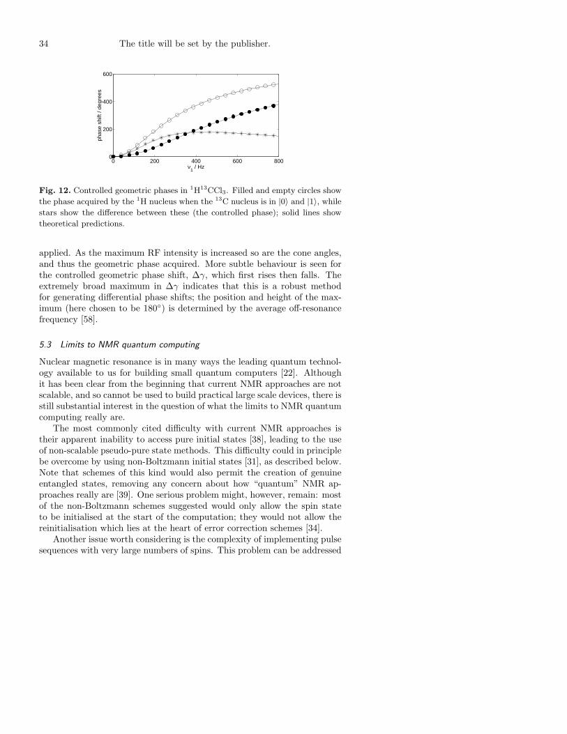
ees
Fig. 12. Controlled geometric phases in 1H13CCl3. Filled and empty circles show
the phase acquired by the 1H nucleus when the 13C nucleus is in |0〉 and |1〉, while
stars show the difference between these (the controlled phase); solid lines show
theoretical predictions.
applied. As the maximum RF intensity is increased so are the cone angles,and thus the geometric phase acquired. More subtle behaviour is seen forthe controlled geometric phase shift, ∆γ, which first rises then falls. Theextremely broad maximum in ∆γ indicates that this is a robust methodfor generating differential phase shifts; the position and height of the max-imum (here chosen to be 180) is determined by the average off-resonancefrequency [58].
5.3 Limits to NMR quantum computing
Nuclear magnetic resonance is in many ways the leading quantum technol-ogy available to us for building small quantum computers [22]. Althoughit has been clear from the beginning that current NMR approaches are notscalable, and so cannot be used to build practical large scale devices, there isstill substantial interest in the question of what the limits to NMR quantumcomputing really are.
The most commonly cited difficulty with current NMR approaches istheir apparent inability to access pure initial states [38], leading to the useof non-scalable pseudo-pure state methods. This difficulty could in principlebe overcome by using non-Boltzmann initial states [31], as described below.Note that schemes of this kind would also permit the creation of genuineentangled states, removing any concern about how “quantum” NMR ap-proaches really are [39]. One serious problem might, however, remain: mostof the non-Boltzmann schemes suggested would only allow the spin stateto be initialised at the start of the computation; they would not allow thereinitialisation which lies at the heart of error correction schemes [34].
Another issue worth considering is the complexity of implementing pulsesequences with very large numbers of spins. This problem can be addressed
Jones: NMR Quantum Computing 35
mathematically by determining how the number of pulses necessary to im-plement a logic gate scales with the size of the spin system; the developmentof efficient refocussing schemes [25, 26] means that the problem scales onlyquadratically, which is reasonable. It is also, however, important to considerpractical questions, such as how individual qubits can be addressed. NMRquantum computing uses the different Larmor frequencies of different spinsto achieve this, and this approach does not scale well, as the frequency spaceavailable is quite limited [31].
Finally it is necessary to consider issues of decoherence. Although NMRdecoherence times can be extremely long compared with other techniques,what matters is not the absolute length of the decoherence time, but ratherthe ratio of the decoherence time to the gate time. Furthermore when es-timating this number it is essential to use the time needed for the slowest
gate in the system, which in NMR systems will correspond to the smallestcoupling used. Experience to date suggests that NMR quantum compu-tations are limited to around 500 gates before the effects of decoherencebecome overwhelming [50, 62]. Note that this number lies well below thevalue required for effective error correction schemes [34].
Putting all these issues together, it seems that the limit to current NMRapproaches lies around 10–15 qubits. While this is far beyond the abilitiesof any currently competing technology, it is not enough to make NMR apractical quantum technology.
5.4 Exotica
Throughout these lectures NMR has been used to refer solely to studies ofspin-half nuclei in liquids and solutions. This restricted field dominates bothconventional NMR studies and NMR implementations of quantum comput-ing for a number of related reasons. There is an obvious way to map qubitsonto spin-half nuclei, and the spin-half Hamiltonian in the liquid state takesa particularly nice form, which is powerful enough to be computationallyuniversal, but simple enough to be easy to work with. Experience fromconventional NMR means that the field is extremely well understood, andthe available technology is highly sophisticated. It is, however, worth brieflyrelaxing these restrictions and seeing what the rest of NMR might have tooffer.
Studying spin-half nuclei in the solid state [12] appears to have manyadvantages. The solid state permits access to very low temperatures, andso the preparation of pure initial states by simple Boltzmann means. Thisdoes not, however, solve the detection problem, or provide a method ofreinitialisation. Solid state samples also retain the full dipolar couplingHamiltonian, which is much larger than the isotropic scalar coupling, andso should allow much faster gates. On the down side, however, dipolarcoupling networks are much more extended than scalar coupling networks,
36 The title will be set by the publisher.
as the dipolar coupling falls off only slowly with distance. Furthermore thehomonuclear dipole-dipole coupling Hamiltonian is not truncated to the(convenient) Ising form. These effects make multiplets extremely broad,rendering selective excitation of individual qubits difficult or impossible.One extreme possibility which has been suggested is to adopt techniquesfrom magnetic resonance imaging to select spins according to their positionsin space, but implementing this will not be easy.
Between liquid and solid state NMR lies the study of molecules in liquidcrystal solvents. These combine some of the features of both extremes,and in particular give some access to dipole-diploe couplings in a controlledmanner. This approach has been used in implementations of NMR quantumcomputing [63,64], but while intriguing it is unlikely to prove important.
Another possibility which has been suggested is to use nuclei with spingreater than one half, usually in the solid state. Such nuclei have both amagnetic dipole moment and a nuclear quadrupole moment, and are oftencalled quadrupolar nuclei [12]. The quadrupole moment will interact withelectric field gradients, and the behaviour of quadrupolar nuclei is dominatedby the interplay between this interaction and the interaction with magneticfields. This can become quite complex, as the relative importance of thetwo interactions varies greatly for different nuclei and for different chemicalenvironments, and the electric field gradient and magnetic field are usuallyattached to quite different reference frames. While this interplay could, inprinciple, be useful, it can also lead to many difficulties, the most obviousexample being rapid dephasing.
Quadrupolar nuclei also have more than two spin states, whcih obviouslysuggests using one spin to store more than one qubit. It is in principlepossible to build a two-qubit device in a single nucleus with spin-3
2 , or evena three-qubit device in a spin-7
2 nucleus. The problem with this approachis, of course, that it does not scale beyond three qubits.
Going beyond nuclei, electrons are spin-half particles, and it should bepossible to perform NMR like experiments using electron spin resonance,or ESR, studies of unpaired electrons in radicals [65]. (ESR is sometimesknown as electron paramagnetic resonance, or EPR.) The electron magneticmoment is much larger than nuclear moments, and so ESR is usually a mi-crowave technique. This also means that pure spin states could be reachedby cooling too the temperature of liquid helium. The theory of ESR looksvery similar to that of NMR, but the experiments are as yet much less de-veloped. Another problem is that radicals with multiple unpaired electronsare very rare, and for this reason most proposals have concentrated on arti-ficial nanostructures. Although this field will be challenging, it is certainlyworth a look.
In the long term one of the most promising techniques is ENDOR, orelectron nuclear double resonance [66], which combines NMR and ESR tech-
Jones: NMR Quantum Computing 37
niques. NMR and ESR have very different energy scales, which makes theexperiments tricky, but may also prove very useful, allowing the high en-ergy scale of ESR to be used for quantum gates, and the low energy scaleof NMR to be used for storage. This is, of course, the ultimate basis of theKane proposal for a large scale quantum computer [67].
5.5 Non-Boltzmann initial states
Although the problem of initialisation is the not the only factor limitingNMR implementations of quantum computing, it remains an importantand annoying problem. The low polarisation of Boltzmann states is alsoan important issue in conventional NMR studies, as it results in a lowsignal strength, greatly limiting the sensitivity of NMR as an analyticaltechnique. For this reason there has long been interest in developing waysto enhance NMR polarisations, and many different techniques have beendeveloped [31]. Of these, however, only two have any realistic prospect ofpreparing essentially pure states: optical pumping, and the use of para-hydrogen.
Optical pumping is, of course, widely used to prepare atoms and ionsin desired electronic states, and these techniques can be extended to pre-pare essentially pure nuclear spin states. Two systems dominate opticallypumped NMR: 3He, which can be pumped directly, and 129Xe and 131Xe,which are pumped indirectly via rubidium atoms. In both cases it is pos-sible to achieve extremely high polarisations, close to unity. However thesenear pure spin states are almost useless for quantum computing, as eachatom can only hold one qubit (or two in the case of the quadrupolar nu-cleus 131Xe), and the atoms do not interact to form molecules. It is possiblein principle to transfer these high polarisations to other nuclei [68], but sofar the efficiency of such transfers has been too low to be useful.
An intriguing alternative is provided by para-hydrogen. This relies onthe fact that the rotational and nuclear spin states of homonuclear diatomicmolecules such as hydrogen are inextricably connected by the Pauli prin-ciple; in particular the even rotational states of hydrogen must have anti-symmetric nuclear spin states. Cooling hydrogen to the rotational groundstate would give pure para-hydrogen with a singlet spin state. As the inter-conversion of ortho and para-hydrogen is forbidden, it is necessary to use acatalyst, but this means that the enhancement will be retained on warmingif the catalyst is removed. Thus it is possible to obtain a bottle of hydrogengas at room temperature with essentially pure nuclear spin states!
It is, of course, not possible to implement quantum computing withpara-hydrogen directly because the hydrogen molecule is too symmetric: itis essential to break the symmetry so that the two nuclei can be addressedindividually. This is easily achieved by adding the para-hydrogen to someother molecule, such as Vaska’s catalyst, to produce a complex where the two
38 The title will be set by the publisher.
1H nuclei have different chemical shifts and so can be separately addressed[69–71]. The addition reaction occurs with retention of nuclear spin state,and so the purity is conserved. In most studies to date, however, the reactionoccurs quite slowly in comparison with the Zeeman frequency differenceof the two spins, leading to dephasing of the off-diagonal elements of thedensity matrix, converting the singlet state to an incoherent mixture of |01〉and |10〉. In conventional para-hydrogen studies this dephasing is accepted,but for NMR quantum computing it is necessary to have fully coherentaddition. One approach used to date [72] is to apply an isotropic mixing
pulse sequence [3], such as mlev-16, which removes the dephasing Zeemaninteraction and preserves the pure singlet spin state. Early experimentsusing this approach have achieved a purity of around 10% in a two qubitsystem [72], significantly below the entanglement threshold. A more recentexperiment has generated systems with a purity of around 86% [73].
6 Summary
Nuclear Magnetic Resonance (NMR) is arguably both the best and the worsttechnology we have for the implementation of small quantum computers.Its strengths lie in the ease with which arbitrary unitary transformationscan be implemented, and the great experimental simplicity arising fromthe low energy scale and long time scale of radio frequency transitions;its weaknesses lie in the difficulty of implementing essential non-unitaryoperations, most notably initialisation and measurement.
The debate over whether NMR quantum computers are “real” quantumcomputers has generated much heat, but also some useful light. It is nowclear that NMR is indeed quantum mechanical, and can in principle beused to build quantum computers, but that the current approach based onpseudo-pure states will never lead to true quantum computing.
Current NMR techniques are not a serious candidate for real quantumcomputing, but NMR remains a great technique for playing around withsmall numbers of qubits. The unparalleled sophistication of NMR will al-most certainly prove a rich source of insights which will find their ultimateapplications in other fields.
A Commutators and product operators
The product operator formalism allows the behaviour of spin systems un-dergoing complicated NMR pulse sequences to be calculated using nothingmore that elementary trigonometry and a table of commutators. A tableof the most important commutators in a two spin system is given below.As an example consider the element in the row labelled Ix and the columnlabelled Iz; the commutator [Ix, Iz] = −iIy and this is entered in the table.
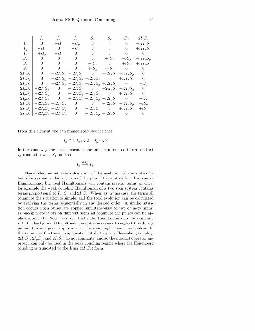
Jones: NMR Quantum Computing 39
Ix Iy Iz Sx Sy Sz 2IzSzIx 0 +iIz −iIy 0 0 0 −i2IySzIy −iIz 0 +iIx 0 0 0 +i2IxSzIz +iIy −iIx 0 0 0 0 0Sx 0 0 0 0 +iSz −iSy −i2IzSySy 0 0 0 −iSz 0 +iSx +i2IzSxSz 0 0 0 +iSy −iSx 0 0
2IxSx 0 +i2IzSx −i2IySx 0 +i2IxSz −i2IxSy 02IxSy 0 +i2IzSy −i2IySy −i2IxSz 0 +i2IxSx 02IxSz 0 +i2IzSz −i2IySz −i2IxSy +i2IxSx 0 −iIy2IySx −i2IzSx 0 +i2IxSx 0 +2iIySz −i2IySy 02IySy −i2IzSy 0 +i2IxSy −i2IySz 0 +i2IySz 02IySz −i2IzSz 0 +i2IxSz +i2IySy −i2IySx 0 +iIx2IzSx +i2IySx −i2IxSx 0 0 +i2IzSz −i2IzSy −iSy2IzSy +i2IySy −i2IxSy 0 −i2IzSz 0 +i2IzSx +iSx2IzSz +i2IySz −i2IxSz 0 +i2IzSy −i2IzSx 0 0
From this element one can immediately deduce that
IxθIz−→ Ix cos θ + Iy sin θ.
In the same way the next element in the table can be used to deduce thatIx commutes with Sx, and so
IxθSx−→ Ix.
These rules permit easy calculation of the evolution of any state of atwo spin system under any one of the product operators found in simpleHamiltonians, but real Hamiltonians will contain several terms at once:for example the weak coupling Hamiltonian of a two spin system containsterms proportional to Iz, Sz and 2IzSz. When, as in this case, the terms allcommute the situation is simple, and the total evolution can be calculatedby applying the terms sequentially in any desired order. A similar situa-tion occurs when pulses are applied simultaneously to two or more spins:as one-spin operators on different spins all commute the pulses can be ap-plied separately. Note, however, that pulse Hamiltonians do not commutewith the background Hamiltonian, and it is necessary to neglect this duringpulses: this is a good approximation for short high power hard pulses. Inthe same way the three components contributing to a Heisenberg coupling(2IxSx, 2IySy, and 2IzSz) do not commute, and so the product operator ap-proach can only be used in the weak coupling regime where the Heisenbergcoupling is truncated to the Ising (2IzSz) form.
40 The title will be set by the publisher.
References
[1] A. Abragam. Principles of Nuclear Magnetism. Clarendon Press, Oxford, UK, 1961.
[2] R. R. Ernst, G. Bodenhausen, and A. Wokaun. Principles of Nuclear Magnetic
Resonance in One and Two Dimensions. Clarendon Press, Oxford, UK, 1987.
[3] R. Freeman. Spin Choreography: Basic Steps in High Resolution NMR. Spektrum,Oxford, UK, 1997.
[4] M. Goldman. Quantum Description of High-Resolution NMR in Liquids. ClarendonPress, Oxford, UK, 1988.
[5] P. J. Hore. Nuclear Magnetic Resonance. Oxford Chemistry Primers, Oxford, UK,1995.
[6] M. H. Levitt. Spin Dynamics: Basics of Nuclear Magnetic Resonance. Wiley,Chichester, UK, 2001.
[7] R. Freeman. Magnetic Resonance in Chemistry and Medicine. Oxford UniversityPress, Oxford, UK, 2003.
[8] T. Claridge. High-resolution NMR Techniques in Organic Chemistry. Pergamon,1999.
[9] R. Freeman. A Handbook of Nuclear Magnetic Resonance. Longman, Harlow, UK,1987.
[10] O. W. Sørensen, G. W. Eich, M. H. Levitt, G. Bodenhausen, and R. R. Ernst. Prog.
Nucl. Magn. Reson. Spectrosc., 16:163–192, 1983.
[11] P. J. Hore, J. A. Jones, and S. Wimperis. NMR: The Toolkit. Oxford ChemistryPrimers, Oxford, UK, 2000.
[12] K. Schmidt-Rohr and H. W. Spiess. Multidimensional Solid-State NMR and Poly-
mers. Academic Press, San Diego, CA, 1994.
[13] E. L. Hahn. Phys. Rev. Lett., 80:580, 1950.
[14] D. P. DiVincenzo. Proc. Roy. Soc. Lond. A, 454:261–276, 1998.
[15] D. Deutsch. Proc. Roy. Soc. Lond. A, 425:73–90, 1989.
[16] D. Deutsch, A. Barenco, and A. Ekert. Proc. Roy. Soc. Lond. A, 449:669–677, 1995.
[17] A. Barenco, C. H. Bennett, R. Cleve, D. P. DiVincenzo, N. Margolus, P. Shor,T. Sleator, J. A. Smolin, and H. Weinfurter. Phys. Rev. A, 52:3457–3467, 1995.
[18] A. Barenco. Proc. Roy. Soc. Lond. A, 449:679–683, 1995.
[19] D. G. Cory, A. F. Fahmy, and T. F. Havel. In T. Toffoli, M. Biafore, and Leao,editors, Proceedings of Phys Comp ’96, pages 87–91. New England Complex SystemsInstitute, 1996.
[20] D. G. Cory, A. F. Fahmy, and T. F. Havel. Proc. Natl. Acad. Sci. USA, 64:1634–1639, 1997.
[21] N. A. Gershenfeld and I. L. Chuang. Science, 275:350–356, 1997.
[22] J. A. Jones. Prog. Nucl. Magn. Reson. Spectrosc., 38:325–360, 2001.
[23] R. Freeman, T. A. Frenkiel, and M. H. Levitt. J. Magn. Reson., 44:409–412, 1981.
[24] E. Knill, R. Laflamme, R. Martinez, and C. H. Tseng. Nature, 404:368–370, 2000.
[25] J. A. Jones and E. Knill. J. Magn. Reson., 141:322–325, 1999.
[26] D. W. Leung, I. L. Chuang, F. Yamaguchi, and Y. Yamamoto. Phys. Rev. A,61:042310, 2000.
[27] J. A. Jones and M. Mosca. Phys. Rev. Lett., 83:1050–1053, 1999.
[28] N. Linden, H. Barjat, and R. Freeman. Chem. Phys. Lett., 296:61–67, 1998.
[29] P. Zanardi and M. Rasetti. Phys. Rev. Lett., 79:3306–3309, 1997.
[30] L. Viola, E. M. Fortunato, M. A. Pravia, E. Knill, R. Laflamme, and D. G. Cory.Science, 93:2059–2063, 2001.
Jones: NMR Quantum Computing 41
[31] J. A. Jones. Fort. der Physik, 48:909–924, 2000.
[32] S. L. Braunstein and H. K. Lo, editors. Scalable Quantum Computers: Paving the
Way to Realisation. Wiley, 2001.
[33] J. A. Jones and M. Mosca. J. Chem. Phys., 109:1648–1653, 1998.
[34] A. M. Steane. Phil. Trans. Roy. Soc. Lond. A, 356:1739–1758, 1998.
[35] J. A. Jones. PhysChemComm, 11, 2001.
[36] J. A. Jones, R. H. Hansen, and M. Mosca. J. Magn. Reson., 135:353–360, 1998.
[37] E. Knill, I. Chuang, and R. Laflamme. Phys. Rev. A, 57:3348–3363, 1998.
[38] W. S. Warren. Science, 277:1688–1689, 1997.
[39] S. L. Braunstein, C. M. Caves, R. Jozsa, Lindenn N., S. Popescu, and R. Schack.Phys. Rev. Lett., 83:1054–1057, 1999.
[40] N. Linden and S. Popescu. Phys. Rev. Lett., 87:047901, 2001.
[41] R. Schack and C. M. Caves. Phys. Rev. A, 60:4354–4362, 1999.
[42] E. Knill and R. Laflamme. Phys. Rev. Lett., 81:5672–5675, 1998.
[43] L. J. Schulman and U. Vazirani. In Proc. 31st ACM STOC, pages 322–329, 1999.E-print quant-ph/9804060.
[44] H. K. Cummins, C. Jones, A. Furze, N. Soffe, M. Mosca, J. M. Peach, and J. A.Jones. Phys. Rev. Lett., 88:187901, 2002.
[45] W. K. Wooters and W. H. Zurek. Nature, 299:802–803, 1982.
[46] V. Buzek and M. Hillery. Phys. Rev. A, 54:1844–1852, 1996.
[47] M. H. Levitt and R. Freeman. J. Magn. Reson., 33:473, 1979.
[48] M. H. Levitt. Prog. Nucl. Magn. Reson. Spectrosc., 18:61–122, 1986.
[49] M. D. Bowdrey, D. K. L. Oi, A. J. Short, K. Banaszek, and J. A. Jones. Phys. Lett.
A, 294:258–260, 2002.
[50] H. K. Cummins and J. A. Jones. New J. Phys., 2:1–12, 2000.
[51] S. Wimperis. J. Magn. Reson. A, 109:221–231, 1994.
[52] H. K. Cummins, G. Llewellyn, and J. A. Jones. Phys. Rev. A, 67:042308, 2003.
[53] R. Tycko. Phys. Rev. Lett., 51:775, 1983.
[54] H. K. Cummins and J. A. Jones. Contemp. Phys., 41:383–399, 2000.
[55] J. A. Jones. Phil. Trans. Roy. Soc. Lond. A, 361:1429–1440, 2003.
[56] J. A. Jones. Phys. Rev. A, 67:012317, 2003.
[57] J. A. Jones. Phys. Lett. A, 316:24–28, 2003.
[58] J. A. Jones, V. Vedral, G. Ekert, and G. Castagnoli. Nature, 403:869–871, 2000.
[59] A. Shapere and F. Wilczek, editors. Geometric Phases in Physics. World Scientific,Singapore, 1989.
[60] M. V. Berry. Proc. Roy. Soc. Lond. A, 392:45, 1984.
[61] A. Y. Kitaev. Annals Phys., 303:2–30. E-print quant-ph/9707021.
[62] L. M. K. Vandersypen, M. Steffen, G. Breyta, C. S. Yannoni, M. H. Sherwood, andI. L. Chuang. Nature, 414:883–887, 2001.
[63] M. Marjanska, I. L Chuang, and M. G. Kubinec. J. Chem. Phys., 112:5095–5099,2000.
[64] B. M. Fung. J. Chem. Phys., 115:8044–8048, 2001.
[65] A. Schweiger and G. Jeschke. Oxford University Press, Oxford, UK, 2001.
[66] M. Mehring, J. Mende, and W. Scherer. Phys. Rev. Lett., 90:153001, 2003.
[67] B. E. Kane. Nature, 393:133–137, 1998.
[68] A. S. Verhulst, O. Liivak, M. H. Sherwood, H. Vieth, and I. L. Chuang. Appl. Phys.
Lett., 79:2480–2482, 2001.

42 The title will be set by the publisher.
[69] C. R Bowers and D. P. Weitekamp. Phys. Rev. Lett., 57:2645–2648, 1986.
[70] J. Natterer and J. Bargon. Prog. Nucl. Magn. Reson. Spectrosc., 31:293–315, 1997.
[71] S. B. Duckett and C. J. Sleigh. Prog. Nucl. Magn. Reson. Spectrosc., 34:71–92,1999.
[72] P. Hubler, J. Bargon, and S. J. Glaser. J. Chem. Phys., 113:2056–2059, 2000.
[73] M. S. Anwar et al. unpublished results, 2003.