Embed Size (px)
Citation preview
STUDY REPORT PHASE 11
CLOSED-LOOP PROCESSING OF
TOPSIDE IONOSPHERIC SOUNDER DATA
C o n t r a c t No, NAS2-4273
Prepared for
NAS A/ARC
Moffett Field, C a l i f .
Prepared by
ASTRODATAl Inc.
240 E. ~Alais Rd,
Anaheim, Calif.
F e b r u a r y 2 0 , 1 9 7 0
P . R. Glen Madsen Study Project M a n a g e r
UNCLASSIFIED
TABLE OF CONTENTS
INTRODUCTION
ACKNOWLEDGMENTS
ABSTRACT
SECTION I FILMCLIP SYSTEM
1 . 0 I n t r o d u c t i o n
1.1 ~ e s c r i ~ t i d n
SECTION I1 INTERPOLATION
2 . 0 I n t r o d u c t i p n
2..1 I n t e r p o l a t i o n of fH
2.2 In terpola t ion of hs
SECTION I11 INVERSE PROCESSING
3 . 0 In t roduct ion
3 . 1 D e s c r i p t i o n
3 . 2 S t e p S e q u e n c e
3 . 3 Mixed Mode
SECTION I V MATRIX PROCESSING
4 . 0 Introduction
4 . 1 D e s c r i p t i o n
4 . 2 S t e p Sequence
4 . 3 C o m p u t a t i o n of h i
P a g e
X
IV- 1
IV- 5
1v-13
IV- 16
TABLE O F CONTENTS (con t )
Page SECTION I V Continued
4 .4 Program NHlYODEL
4 - 5 The Pseudoinverse
SECTION V
APPENDIX
NOR1 ZONTAL PROCESSING
5.0 In t roduc t ion
5 .1 Horizontal Inverse Processing V-4
5.2 Horizontal Matrix Processing V-9
Technical Reports
TR-1 Some Proposed Methods f o r Reduction o f Topside Ionograms to ' E l e c t r o n i c Density P r o f i l e s
TR-2 A Weighted Leas t Square Approximation Method
TR-3 Xnverse Mapping t o Spec i f i ed f
TR-4 S i m p l i f i c a t i o n of Matrix Inverse Problem
TR-5 Time Skew Problem
TR-6 Optimal S tep S ize by One Dimensional Search
TH-7' Horizontal Processing
TR-8' Computation of t h e Pseudoinverse
iii

LIST OF ILLUSTRATIONS
F i g u r e T i t l e
NASA/ARC FILMCLLP System
F u n c t i o n a l Block Diagram - A s t r o d a t a S c a l i n g
C o n v e r t e r
Cross S e c t i o n - S a t e l l i t e O r b i t a l P l a n e
P a r a b o l i c I n Log N R e p r e s e n t a t i o n
Mapping of P o i n t s i n h v f ) P l a n e Above and B e l o w
t h e X-Trace
Mapping o f P o i n t s I n h s ( f ) P l a n e A l l o n One S i d e
of X-Trace
Flow Diagram - I n v e r s e P r o c e s s i n g
Zero/Pole R e p r e s e n t a t i o n o f N (h) P r o f i l e
Mapping o f Cor respond ing P o i n t s i n t h e h ' (f)
a n d N(h) P l a n e s
Flow Diagram - N(h,.) P r o c e s s i n g M a t r i x Method
Flow Diagram - To Compute hi f o r M a t r i x P r o c e s s i n g
Goldell S e c t i o n S e a r c h
Flow Diagram f o r Program NHMODEL
MFIMQDEL Flow Diagram - S u b r o u t i n e CALC [AMC, HN, S, ZK]
NkIMODUL Flow Diagram - S u b r o u t i n e GEND [D,S,ZK]
NfIMODEL Flow Diagram - S u b r o u t i n e MXV [A, X, B,T,N,Nl]
NIIMODEL Flow Diagram - S u b r o u t i n e COST [AMP,E, HN, ZK,
EMAX, EXM]
Figu re
4-11
T i t l e
NHMODEL Flow D i a g r a m - Subrou t ine STEP [ALVIP,DK,E,
HN, S , ZK,EMAX, EXM,QS]
R e p r e s e n t a t i v e N (h, t) P r o f i l e s f o r Two Consecu t ive
Ionograms
REFERENCES
[ ''L. Colin, K. L. Chan, R. G. Madsen, "FILMCLIP, Closed-Loop
Ionogram Processor for the Analysis of Topside Sounder Ionogram
Films," to be published, 1970.
[ W. Cooper "Scaling Converter Format for Closed-Loop-Ionogram-
Processor (CLIP)", Informatics Pr~ject 780 - Technical Note 101, May 3, 1968.
1 3 ' J. G. K. Lee, "Computations of Satellite Position and Gyro-
frequency for the Closed-Loop-Ionogram-Processor (CLIP)",
Informatics Project 780 - Technical Note 103, May 14, 1968.
['"J. G. K. Lee, "Computations of Satellite Position and Gyro-
frequency for the Closed Loop Ionogram Processor", Informatics
Project 780 - Technical Note 104, May 20, 1968.
["J. G. K. Lee. "Computation of Satellite Position and Gyro-
frequency for the Closed-Loop-Ionogram-Processor (CLIP)",
Informatics Project 780 - Technical Note 105, June 3, 1968-
[ 6 1 ~ . G. K. Lee, W. R . Cooper, G . Slike, R. G. Madsen, "Description
of Programncd Function Keys for Closed-Loop-Ionogram-Processor
( C L I P ) ", :Infor-tnntics Project 780 - Technical Note 102, May 24, 1968.
'I G. S l i k e , "FILMCLIP 1 8 0 0 P r o g r a m D o c u m e n t a t i o n , " I n f o r m a t i c s
TR-1064-5-3, J a n u a r y 2 3 , 1 9 6 9 .
W. R. C o o p e r , "FILMCLIP Summary, It I n f o r m a t i c s TR-1064-5-1,
F e b r u a r y 5 , 1 9 6 9 .
" ' G . S l i k e , J. G . K. L e e , "FILMCLIP U s e r ' s G u i d e , I n f o r m a t i c s
TR-1064-5-4, F e b r u a r y 5, 1 9 6 9 .
J. G . K. L e e , "FILMCLIP 360 P r o g r a m D o c u m e n t a t i o n , " ~ n f o r r n a t i c s
TR-1064-5-2, FIay 2 9 , 1 9 6 9 .
[ ' ' l id. R. C o o p e r , G. S l i k e , J. G. K . L e e , "CLIP-An interactive
M u l t i - C o m p u t e r S y s t e m f o r P r o c e s s i n g I o n o s p h e r i c D a t a , "
A I M P a p e r N o . 6 9 - 9 5 2 , AIAA A e r o s p a c e C o m p u t e r S y s t e m s
C o n f e r e n c e , L o s A n g e l e s , C a l i f . , S e p t e m b e r 8 -10 , 1 9 6 9 .
[12]~s t rodata, I n c . , " S c a l i n g C o n v e r t e r , " I n s t r u c t i o n Manual,
P ro j ec t 9 3 8 4 0 0 , J a n u a r y 3 0 , 1 9 7 0 .
1 ' ' 1 ,1. k:. l l , ~ c k a o r ~ , "l'llr Fieduct ion o f Topsj do lonograms to E l ectrsn-
Uc?llui ty Prof i l e a , " Proc. Il"lb::E, J u n e 19 69. --
["] 3. E. J a c k s o n , " C o m p a r i s o n B e t w e e n T o p s i d e a n d G r o u n d - B a s e d
S o u n d i n g s , " P r o c . IEEE, June 1 9 6 9 . L _ _

[ 1 5 ] ~ . E. K. Lockwood. "A Modified I t e r a t i o n Technique f o r u s e i n
Computing E l e c t r o n Densi ty P r o f i l e s from Topside Ionograms,"
Accepted f o r p u b l i c a t i o n i n Radio Sc ience .
[ 1 6 ] ~ . G. Madsen, A. F. Sca rd ina , N. L. D a w i r s , "Engineer ing Study
and P re l imina ry Design of In s t rumen ta t ion f o r t h e S c a l i n g
and E d i t i n g of Ionograph D a t a , " As t roda t a , I n c a Study Report ,
Phase I P a r t I , Con t r ac t N o . NAS2-4273, November 1967.
[ I 7 ] 5 . G. K. Lee, "Reduction o f A loue t t e I1 Topside Ionograms t o
E l e c t r o n Densi ty P r o f i l e s , " Program Documentation f o r NASA/ARC,
[ l R 1 J * G . K. L e e , "Reduction of E l e c t r o n Densi ty P r o f i l e s t o
A loue t t e I1 Topside Ionograms," Program Documentation f o r
NASA/ARC, 19 6 7 .
[ l g l ~ . C. K . Lee, "Optimal Es t ima t ion , I d e n t i f i c a t i o n , and C o n t r o l , "
Research Monograph No. 28 , The M.I.T. P r e s s , 1964.
[''I D . D. PlcCracken, " F o r t r a n w i t h Engineer ing App l i ca t ions , "
Wiley, 1367.
v i i i
The fo l lowing r e f e r e n c e s are i n t h e Appendix:
rZ1l J. E* Kinkel "Some Proposed Methods f o r Reduction o f Topside
Ionograms t o E l e c t r o n Dens i ty P r o f i l e s , " As t roda ta P r o j e c t
938400 - Technica l Report 1, September 25 , 1969,
[221 J. F Kinkel , "A Weighted L e a s t Squares Approximation Method, "
Ast roda ta P r o j e c t 938400 - Technica l Report 2 , November 2 1 ,
1969.
'231 J. F. Kinkel , " I n v e r s e Mapping t o S p e c i f i e d f , " As t roda t a
P r o j e c t 938400 - Technica l Report 3 , November 2 4 , 1969.
12*] J. F. Kinkel , " S i m p l i f i c a t i o n o f Matr ix Inve r s ion Problem, "
Ast roda ta P r o j e c t 938400 - Technica l Report 4 , December 1, 1969.
[2 51 J. F. K i n k e l , "Time Skew Problem," As t roda t a P r o j e c t 938400 -
I
Technica l Report 5 , December 12, 1969.
[''I J. F e Kinkel , "Optimal S t e p S i z e by One Dimensional Sea rch , "
As t roda t a P r o j e c t 938400 - Technica l Report 6,. December 30, 1969.
'271 J. F * Kinkel , "Hor izonta l P roces s ing , " ~ s f r o d a t a P r o j e c t 938400 - Technica l Report 7 , January 30, 1970.
[' J. . Kinkel , "Computation o f . t h e Pseudoinverse , " A s t r o d a t a
Project 938400 - 'Technical Eicport 8 , February 16 , 1970.
INTRODUCTION
The Phase I1 Study was undertaken t o i n v e s t i g a t e t h e closed-loop
da ta reduct ion techniques descr ibed i n t h e f i r s t Study Report [I61
and t o i n v e s t i g a t e some new ideag t h a t had evolved s i n c e t h a t
r e p o r t was w r i t t e n . With t h e a v i i l a b i l i t y of t h e computer hardware
a t NASA/ARC, it requ i red only the a d d i t i o n of t h e i n t e r f a c e
hardware between t h e Oscar-F Data Reader and t h e Computer, p lus
the a s soc ia ted sof tware , t o impLsment what was i n i t i a l l y c a l l e d
the Phase I1 s imula tor . This s imula tor has now become t h e FILMCLIP
System which has provided NASA/ARC w i t h closed-loop ionogram
processing c a p a b i l i t y s i n c e September 1968. Since t h a t d a t e ,
many thousands of tops ide ionograms have been reduced t o e l e c t r o n
dens i ty p r o f i l e s , including, high a l t i t u d e ionograms t h a t cannot
be processed on an open-loop b a s i s . The FILMCLIP System w i l l
cont inue t o be used i n t h e development of new computational
sof tware t h a t is descr ibed i n t h i s r e p o r t .
Astroda ta e x p r e s s e s i t s a p p r e c i a t i o n t o D r . Lawrence C o l i n and
D r . K. L. Chan o f NASA/ARC f o r t h e i r c o n t r i b u t i o n s t o and
guidance o f t h i s Study e f f o r t .
The S c a l i n g Conver te r i n t h e FILMCLIP System was des igned and
b u i l t by Ed Haske, Fred Mata, and E l i z a b e t h S t a r r .
Software development f o r t h e FILMCLIP System was provided by
Glenn S l i k e , J ack Lee, Will iam Burns, Wilson Cooper and Gera ld ine
l\lcCulley o f In fo rma t i c s , Inc . Improvements i n t h e N ( h ) computat ional
so f tware were made by Leonard McCulley of In fo rma t i c s , I nc .
T h e c o n t r i b u t i o n s of John Kinkel i n t h e development o f t h e Inve r se ,
Matr ix , and Hor i zon ta l P roces s ing methods a r e g r a t e f u l l y acknowledged.
Spec i a l thanks are due Grace Eckmark f o r h e r h e l p i n o p e r a t i n g t h e
t ime s h a r e computing t e r m i n a l , and f o r t y p i n g t h e r e p o r t . Also
t l m ~ - ~ l c s t o M,zry 1 l . i . L l m c r for i n c o t p o r a t i n c . ~ Lhc. c o r r c ~ c t i o n s atld
~ k 1 . i L ~ l i i l l CI~LIY~~_FC?S. '1'11~ ' r @ p c ) r t W A S cdi tcd by Don W i l lcy .
ABSTRACT
High a l t i t u d e t o p s i d e ionosphe r i c sounder d a t a i s be ing provided
from both t h e A l o u e t t e I1 and ISIS-1 sa te l l i t es . The r e s u l t i n g
ionograms are f r e q u e n t l y s o d i f f i c u l t t h a t open-loop p roces s ing
techniques a r e inadequa te t o cope wi th t h e problem. Closed-loop
d a t a r e d u c t i o n methods o f f e r a p r a c t i c a l s o l u t i o n t o t h e problem
of reduc ing ionograms from h igh a l t i t u d e soundings , and a t t h e
same t ime provide improved c a p a b i l i t y f o r p roces s ing a l l ionograms.
The FILMCLIP System i s a Closed-Loop Ionogram Processor f o r t h e
reduc, t ion o f t o p s i d e ionosphe r i c sounder d a t a recorded on 3 5 m
Film. Th i s system was implemented a t NASA/ARC a s p a r t o f a
con t inu ing s tudy t o develop methods o f automat ing t h e d a t a r e d u c t i o n
of t o p s i d e ionograms. The system h a s worked s o w e l l t h a t it i s
now used n e a r l y f u l l t i m e f o r f i l m ionogram d a t a r e d u c t i o n on a
p roduc t ion b a s i s .
The f i n a l d a t a r e d u c t i o n system, which w i l l a c q u i r e i n p u t d a t a
d i r e c t l y from magnet ic t a p e , i s known a s t h e TAPEGLIP System.
Software is be ing developed f o r t h e TAPECLIP System t h a t w i l l u se
much of t h e e x i s t i n g so f tware . T h i s s o f t w a r e i s organized
t o g e t h e r w i th new s o f t w a r e t o e x p l o i t t h e new c losed- loop
p roces s ing techniques t h a t a r e now a v a i l a b l e . The TAPECLIP
sof twnre i.s being developed and checked o u t under s imula ted
conci i t ions 01.1 the F'ILFlCLIP System.
A number o f d i f f e r e n t methods f o r computing e l e c t r o n d e n s i t y
p r o f i l e s from tops ide ionospher ic sounder d a t a a r e presented.
The method of Inverse processing i s a v a r i a t i o n of Jackson's ~ 3 1
parabo l i c i n log N laminat ion method. Lamination h e i g h t s a r e
p rese lec ted a t equa l ly spaced increments of t r u e he igh t . The
sca led X-Trace d a t a is curve f i t so t h a t t h e v i r t u a l depth, hi,
i s known f o r any frequency f on t h e X-Trace. The plasma frequency
f N i s t h e n ad jus ted i n an i t e r a t i v e procedure f o r each laminat ion
boundary u n t i l computed p o i n t s i n t h e h ' ( f ) p lane match t h e curve
f i t X-Trace,
Inverse mixed-mode processing provides a way f o r au tomat ica l ly
combining sca led d a t a from both t h e X and 0-Traces t o provide a
composite e l e c t r o n d e n s i t y N (h) p r o f i l e .
The Matrix method of ionogram d a t a reduct ion uses an a n a l y t i c
model of t h e N(h) p r o f i l e . I n t h i s method t h e c o e f f i c i e n t s o f a
mathematical model o f t h e N(h) p r o f i l e a r e ad jus ted t o minimize
t h e e r r o r between scaled and computed va lues of h q ( f . ) i n a 1
w e i g h t e d Icast squares sense ,
The method of ISorizonCal processing provides a means f o r f i r s t
o rde r c o r r e c t i o n of t h e e f f e c t s of hor i zon ta l g r a d i e n t s o f
e l e c t r o n d e n s i t y i n t h e s a t e l l i t e o r b i t a l plane. The method of
Horizontal processing recognizes t h a t the tops ide sounder ionogram
x i i i
d a t a and t h e r e s u l t a n t computed e l e c t r o n d e n s i t y p r o f i l e a r e
both func t ions of time due t o t h e s a t e l l i t e v e l o c i t y wi th
r e spec t t o e a r t h based coordina tes ,
New subrout ines t h a t w e r e developed i n t h e course of opt imizing
some of t h e computational sof tware a s fol lows:
a . Inverse mapping t o s p e c i f i e d f
b. S impl i f ied s o l u t i o n of a mat r ix equat ion
c . Optimal s t e p s i z e by Golden Sect ion Search
d . Matrix pseudoinverse computation
The weighted l e a s t squares approximation method of Mall inckrodt
was u t i l i z e d i n t h e matr ix method.
An i n v e s t i g a t i o n was conducted t o show t h a t values of fH, 4 , and
hS between accura te ly computed po in t s could be obtained by
i n t e r p o l a t i o n . The use of i n t e r p o l a t i o n has g r e a t l y reduced t h e
computer work load i n t h e determinat ion of values f o r these
p~%r;+-imctcrs .
SECTION I
FILMCLIP SYSTEM
1.0 INTRODUCTION
The FILMCLIP System is a Closed-Loop Ionogram Processor t h a t is
now i n use on a p roduc t ion b a s i s f o r t h e r e d u c t i o n of t o p s i d e
ionosphe r i c sounder d a t a recorded on 35 mrn f i l m . The FILMCLIP
System was implemented i n September 1968 on a minimum
c o s t b a s i s as p a r t of a c o n t i n u i n g s tudy f o r NASA/ARC on advanced
equipment and techniques f o r t o p s i d e ionosphe r i c sounder d a t a
r educ t ion . S i n c e t h a t d a t e many thousands o f ionograms have been
reduced t o e l e c t r o n d e n s i t y p r o f i l e s , i n c l u d i n g ionograms from
h igh a l t i t u d e low d e n s i t y soundings . The l a t t e r a r e almost
imposs ib le t o reduce on an open l o o p b a s i s due t o t h e d i f f i c u l t i e s
involved i n i d e n t i f y i n g t h e p o r t i o n of t h e X-Trace due t o v e r t i c a l
p ropaga t ion .
I n early 1968, the Computation Div i s ion a t NASA/AR@ made a v a i l a b l e
an IRM 1800 Computer, I B M 2250 Graphic Display Un i t , and I W M 360/50
Comput,er t o the Space Sc iences D iv i s ion on a second s h i f t ,
non - in t e r f e r ence b a s i s . With t h e a v a i l a b i l i t y of t h i s computing
equipment, As t roda t a proposed t h a t a Phase I1 s i m u l a t o r b e
implemented a t NASA/ARC us ing t h e e x i s t i n g Oscar-F d a t a r e a d e r
and t h e above computers t o p rov ide a c losed- loop f i l m ionogram
p roces s ing c a p a b i l i t y f o r i n v e s t i g a t i n g advanced p roces s ing
a lgo r i t hms , and f o r reduc ing f i l m ionograms on a p roduc t ion b a s i s . a
The follow-on s tudy f o r t h e development of improved tops ide
ionogram d a t a r educ t ion methods has a number of o b j e c t i v e s as
follows:
a . fmproved closed-loop process ing methods which t ake
advantage o f some o f t h e newer opt imiza t ion techniques.
b e Relegate more o f t h e ionogram p a t t e r n r ecogn i t ion t a s k
t o computer sof tware.
c . Take b e t t e r advantage of a l l t h e d a t a i n an ionogram
f o r production ionogram d a t a reduct ion .
d. Correc t ion of known d e f i c i e n c i e s i n e x i s t i n g d a t a
r educ t ion methods.
e, U s e t h e FILMCLIP System a s a s imula tor f o r development
of TAPECLIP d a t a reduct ion software.
1.1 DESCRIPTION
'9'he FSLMCLIP System is a n on- l ine i n t e r a c t i v e computer processing
system that has been o p e r a t i o n a l a t NASA/ARC s i n c e September 1968.
A func t iona l block diagram of t h e FILMCLIP System i s shown i n
Fig . 1-1. The performance c h a r a c t e r i s t i c s of t h e FILMCLIP
System were def ined by Astrodata and t h e d e t a i l s worked o u t i n a
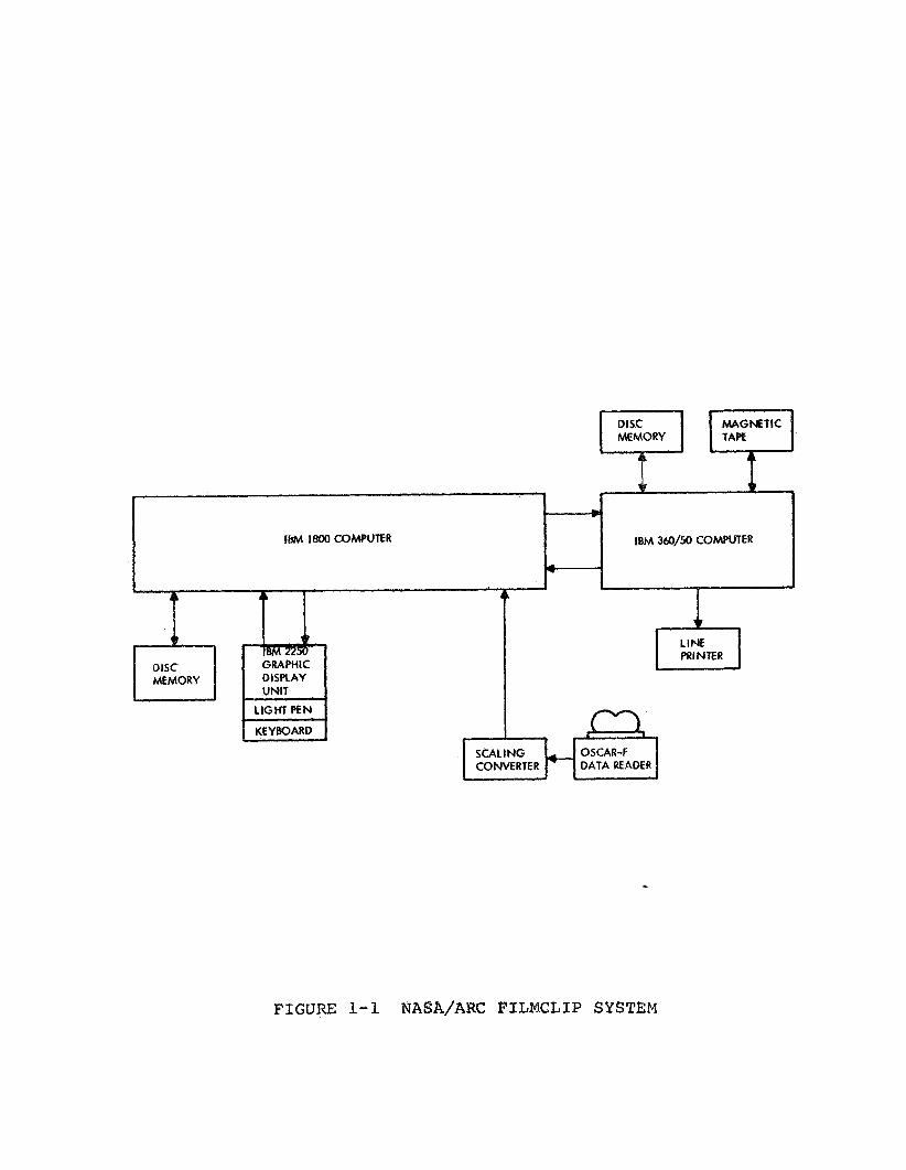
tbM 1800 COMPUTER IBM 360/50 COMPUTER
series o f con fe rences w i t h MASA/ARC and In fo rma t i c s , Inc . The
o p e r a t i o n a l so f tware f o r t h e s y s t e h w a s provided by In fo rma t i c s ,
A number o f t e c h n i c a l r e p o r t s and' pape r s have been w r i t t e n a b o u t [ 1 - 1 1 1
t h e FILKLIP System t o which t h e reader i s d i r e c t e d f o r
s p e c i f i c d e t a i l e d in format ion .
The S c a l i n g Conver ter i n t h e system w a s b u i l t by Astrodata as a
p i e c e o f i n t e r f a c e hardware between t h e Oscar-F data r e a d e r anq
t h e IBM 1800 Computer. A f u n c t i o n a l b lock diagram of t h e S c a l i n g
Converter i s shown i n Fig . 1 - 2 . A detailed d e s c r i p t i o n o f t h i s
" u n i t , i n c l u d i n g l o g i c diagrams and schemat ics , i s conta ined i n
t h e I n s t r u c t i o n Manual. [ 1 2 1

FUNCTIONAL BLOCK DIAGRAM
SCALING CONVERTER
FIGURE 1-2
SECTION I1
INTERPOLATIOEJ
2.0 INTRODUCTION
S i g n i f i c a n t s av ings i n computer t i m e can be achieved by s imple
i n t e r p o l a t i o n of parameter v a l u e s between a c c u r a t e l y computed
p o i n t s , compared w i t h d i r e c t computation of t h e parameters each
t ime new va lues a r e needed. The f e a s i b i l i t y of i n t e r p o l a t i n g
i n t e r m e d i a t e va lues of gyrofrequency f H and s a t e l l i t e h e i g h t hS
were i n v e s t i g a t e d . The d i p ang le f3 changes s o s lowly t h a t tests f o r
i n t e r p o l a t i o n accuracy f o r 8 w e r e n o t i nc luded i n t h i s i n v e s t i g a t i o n .
I n t h e d a t a r e d u c t i o n o f t o p s i d e ionograms t o e l e c t r o n d e n s i t y
p r o f i l e s , t h e X-Trace i s used a lmos t e x c l u s i v e l y . This i s
p r i m a r i l y t r u e because t h e X-Trace is n e a r l y always cont inuous
a t t h e low frequency end down t o t h e c u t o f f f requency, wh i l e t h e
low frequency end of t h e 0-Trace is u s u a l l y miss iny . S incc t h e
ref'lcct:.i.on p o i n t of t l ~ c ! extraordinary wave i s dependent on both
the e l e c t r o n d e n s i t y N and t h e f l u x d e n s i t y B of t h e e a r t h ' s
magnetic f i e l d , it is necessary t o compute va lues o f t h e e a r t h ' s
magnetic f i e l d each t i m e t h e group path i n t e g r a l i n egn. (2-1) 11 33
i s eva lua t ed .
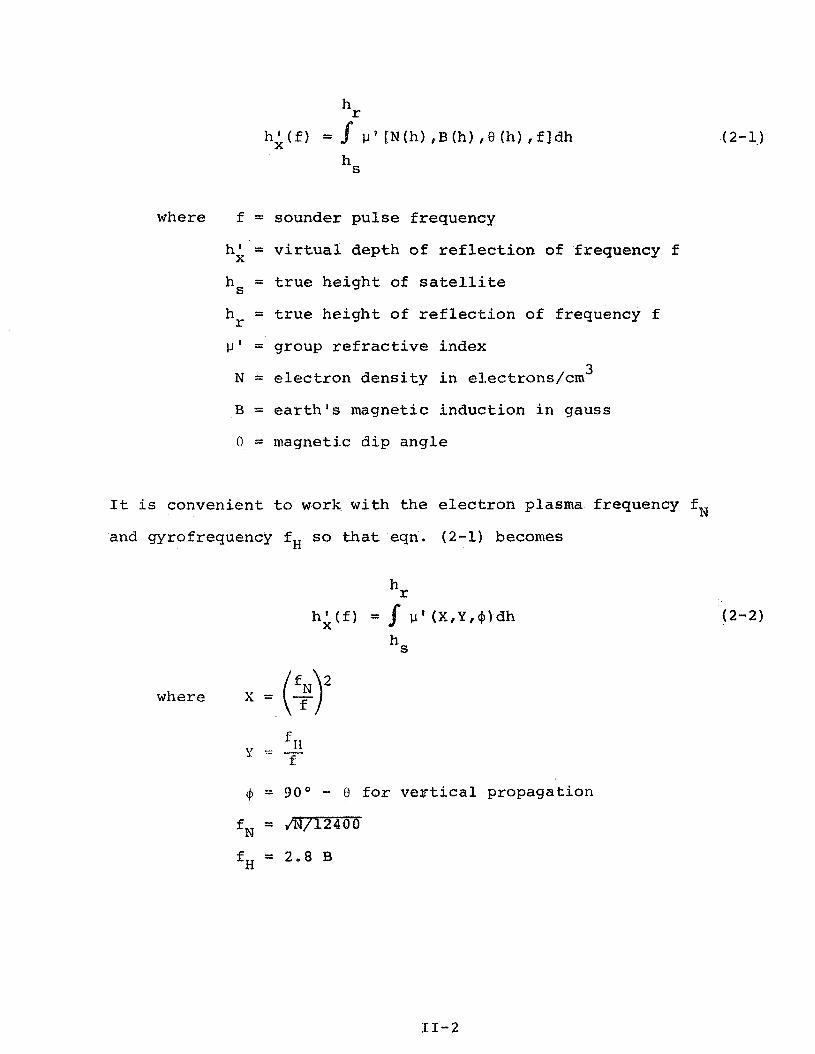
where f = sounder p u l s e f requency
h& = v i r t u a l dep th o f r e f l e c t i o n of f requency f
hs = t r u e h e i g h t of s a t e l l i t e
hr = t r u e h e i g h t of r e f l e c t i o n of f requency f
p ' = group r e f r a c t i v e index
N = e l e c t r o n d e n s i t y i n e lec t rons /cm 3
B = e a r t h ' s magnet ic i n d u c t i o n i n gauss
0 = magnetic d i p a n g l e
I t is convenien t t o work w i t h t h e e l e c t r o n plasma frequency fN
and gyrofrequency fH s o t h a t eqn. (2-1) becomes
4 = 90' - O f o r v e p t i c a l p ropaga t ion
D i r e c t computation o f t h e geomagnetic f i e l d a s a sub ta sk i n t h e
e v a l u a t i o n of t h e group pa th i n t e g r a l t a k e s a s i g n i f i c a n t amount
of computer t i m e . his computation is based on a s p h e r i c a l
harmonic expansion r e p r e s e n t a t i o n of t h e f i e l d w i th c o e f f i c i e n t s
from Danie l s and Cain. 71
I n an e f f o r t t o reduce t h e number of d i r e c t computations o f t h e
geomagnetic f i e l d , a t a s k w a s set up t o e v a l u a t e t h e p o s s i b i l i t y
of us ing i n t e r p o l a t i o n a s a means f o r de te rmin ing t h e gyro-
frequency. T h e o b j e c t i v e o f t h e t a s k was t o p rov ide a comparison
between d i rcc t1 .y computed and i n t e r p o l a t e d va lues of f H .
A c r o s s s e c t i o n of t h e s a t e l l i t e o r b i t a l p l ane was set up as
shown i n P ig . 2-1 w i t h boundar ies 400 km a p a r t v e r t i c a l l y between
200 k m and 3000 k m , and approximately 220 km a p a r t h o r i z o n t a l l y ,
which i s t h e average d i s t a n c e t h e A l o u e t t e I1 sa te l l i te t r a v e l s ---
between cor responding f requency markers from one ionogram t o
t h e nex t . The t i m e between cor responding f requency markers i s
approximately 31 seconds, and t h e p e r i o d of u s e f u l d a t a cove r s
r o u g h l y o n e - h a l f tllc ionogram which i s abou t 1 p a r t i n 500 o f
thc o r b i t a l pe r iod . From t h i s it i s r ea sonab le t o assume t h a t
the v e l o c i t y of t h e s a t e l l i t e i s e s s e n t i a l l y c o n s t a n t o v e r t h e
pe r iod of t h e X-Trace, s o t h a t l i n e a r i n t e r p o l a t i o n of f H w i t h
r e s p e c t t o t ime a t c o n s t a n t h e i g h t should b e f e a s i b l e .
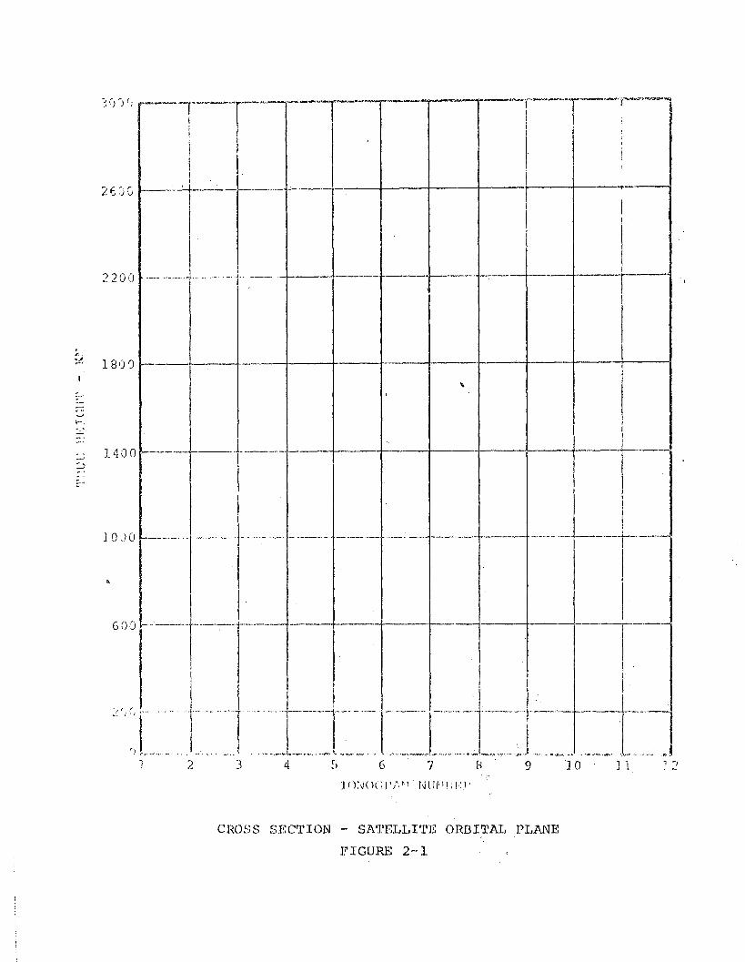
CROSS SECTION - SATELLITE ORBITAL PLANE
FIGURE 2-1
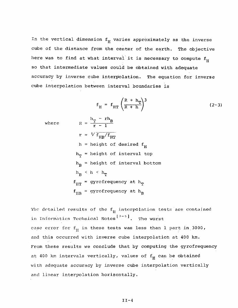
I n t h e v e r t i c a l dimension f H v a r i e s approximately a s t h e i n v e r s e
cube o f t h e d i s t a n c e from t h e c e n t e r of t h e e a r t h . The o b j e c t i v e
h e r e w a s t o f i n d a t what i n t e r v a l it is neces sa ry t o compute fH
s o t h a t i n t e r m e d i a t e va lues could be o b t a i n e d w i t h adequa te
accuracy by i n v e r s e cube i n t e r p o l a t i o n . The equa t ion f o r i n v e r s e
cube i n t e r p o l a t i o n between i n t e r v a l boundar ies is
where
h = h e i g h t o f d e s i r e d f H
hT = h e i g h t o f i n t e r v a l t o p
hB = h e i g h t of i n t e r v a l bottom
hB < h < hT
fHT = gyrofrequency a t hT
HB = gyrofrequency a t hB
'k'lic dc t a i led r e s u l t s of t h c f i n t e r p o l a k i o n test,;; a r c con.tc1.i ned I I [ 3 - 5 1
i n i n f ~ r m ~ ~ t i c s Tccllnical Notes . ?'he wors t
case e r r o r fo r f H i n t h e s e tests was less than 1 p a r t i n 3000,
and t h i s occur red w i t h i n v e r s e cube i n t e r p o l a t i o n a t 400 km.
From t h e s e r e s u l t s w e conclude t h a t by computing t h e gyrofrequency
a t 400 km i n t e r v a l s v e r t i c a l l y , v a l u e s of f H can be ob ta ined
w i t h adequate accuracy by i n v e r s e cube i n t e r p o l a t i o n v e r t i c a l l y
and i i n e a r i n t e r p o l a t i o n h o r i z o n t a l l y ,
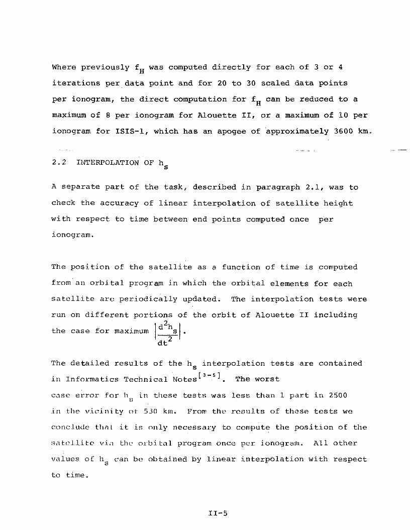
Where previous ly f H was computed d i r e c t l y f o r each of 3 o r 4
i t e r a t i o n s per d a t a p o i n t and f o r 20 t o 30 sca led d a t a p o i n t s
per ionogram, t h e d i r e c t computation f o r f H can be reduced t o a
maximum of 8 pe r ionogram f o r Alouet te 11, o r a maximum of 10 pe r
ionogram f o r ISIS-1, which has an apogee of approximately 3600 km.
2 . 2 INTERPOLATION OF hs
A sepa ra te p a r t of t h e t a s k , descr ibed i n paragraph 2 . 1 , was t o
check t h e accuracy of l i n e a r i n t e r p o l a t i o n of s a t e l l i t e h e i g h t
with r e s p e c t t o time between end p o i n t s computed once p e r
ionogram.
T h e p o s i t i o n of t h e s a t e l l i t e as a funct ion of time is computed
from a n o r b i t a l program i n which t h e o r b i t a l elements f o r each
s a t e l l i t e a r e p e r i o d i c a l l y updated. The i n t e r p o l a t i o n tests w e r e
run on d i f f e r e n t por t ions of t h e o r b i t of Alouet te I1 inc luding
the case f o r maximum d2hs
The d e t a i l e d r e s u l t s of t h e hs i n t e r p o l a t i o n t e s t s a r e contained
i n Informatics Technical Notes 1 3 - 5 3 The wors t
case error for h i n these tests w a s less than 1 p a r t i n 2500 s
i n t t ~ e vie-ir~ity o f 530 km. From thc r e s u l t s o f t hese tests we
roncludc thn t i t i.s c.7111~ necessary to con~putc the p o s i t i o n of the
S i i tc?l l i tc. v i , I t.hc5 01 b i t -n l program once per ionograin. A 1 1 o t h e r
v a l u e s of hs can be obtained by l i n e a r i n t e r p o l a t i o n w i t h r e spec t
t o time,
SECTION I11
INVERSE PP,OCESSING
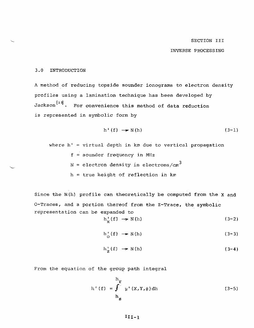
3 . 0 INTRODUCTION
A method of reduc ing t o p s i d e sounder ionograms t o e l e c t r o n d e n s i t y
p r o f i l e s u s ing a l amina t ion technique h a s been developed by
~ a c k s o n ' l ~ ] . For convenience t h i s method of d a t a r educ t ion
i s r e p r e s e n t e d i n symbolic form by
where h ' = v i r t u a l depth i n km due t o v e r t i c a l p ropaga t ion
f = sounder frequency i n MHz
N = e l e c t r o n d e n s i t y i n e lec t rons /cm 3
h = t r u e h e i g h t of r e f l e c t i o n i n km
Since t h e N(h) p r o f i l e can t h e o r e t i c a l l y b e computed from t h e X and
0-Traces, and a p o r t i o n the reo f from t h e 2-Trace, t h e symbolic
r e p r e s e n t a t i o n can be expanded t o h;(f) --r N(h) (3 -2 )
From the equa t ion of t h e group pa th i n t e g r a l
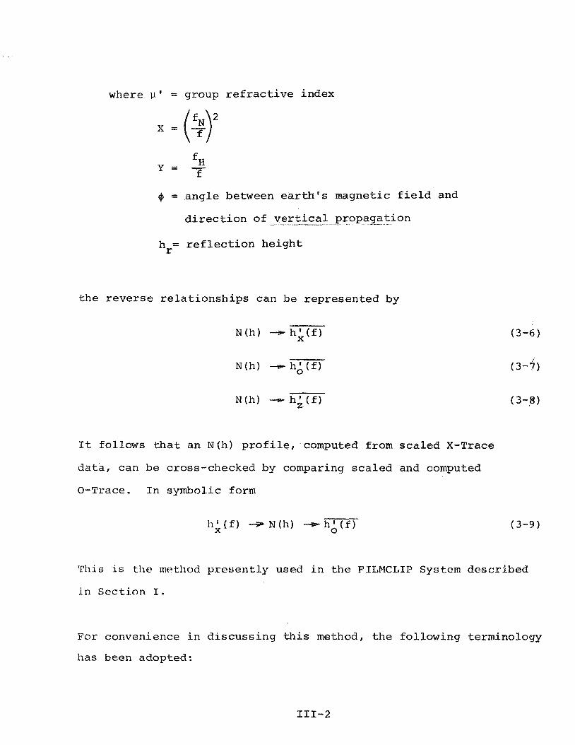
where p' = group r e f r a c t i v e index
+ = angle between e a r t h ' s magnetic f i e l d and
d i r e c t i o n of -- v e r t i c a l -- -- propagat ion . -
hr= r e f l e c t i o n he igh t
t h e r eve r se r e l a t i o n s h i p s can be represented by
I t follows t h a t an N(h) p r o f i l e , computed from sca led X-Trace
d a t a , can be cross-checked by comparing sca led and computed
0-Trace. I n symbolic form
I ') I l l i s is tllc rnethod p r e s e n t l y used in t 1 . 1 ~ FILMCLIP System described
i n S e c t i o n I .
For convenience i n d i s c u s s i n g t h i s method, t h e fol lowing terminology
has been adopted:
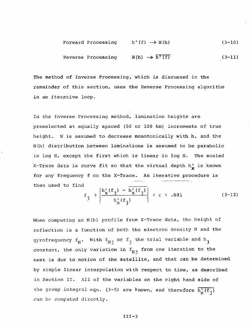
Forward P roces s ing h' ( f ) 4 N(h)
Reverse P roces s ing N(h) + h' (f)
The method of I n v e r s e Process ing , which is d i scussed i n t h e
remainder o f t h i s s e c t i o n , u se s t h e Reverse Process ing a lgo r i t hm
i n an i t e r a t i v e loop .
I n the Inve r se P roces s ing method, l amina t ion h e i g h t s a r e
p r e s e l e c t e d a t e q u a l l y spaced (50 o r L O O km) increments o f t r u e
h e i g h t . N is assumed t o dec rease monotonical ly wi th h , and t h e
N(h) d i s t r i b u t i o n between l amina t ions i s assumed t o b e p a r a b o l i c
i n l o g N , excep t t h e f i r s t which i s l i n e a r i n l o g N. The s c a l e d
X-Trace d a t a i s curve f i t s o t h a t t h e v i r t u a l dep th h i is known
f o r any f requency f on t h e X-Trace. An i t e r a t i v e procedure is
then used t o f i n d
When computing an N ( h ) profi1.e from X-Trace d a t a , t h e h e i g h t of
r e f l e c t i o n i s a f u n c t i o n of bo th t h e e l e c t r o n d e n s i t y N and t h e
qyrofrequcncy fH. With f o r f t h e t r i a l v a r i a b l e and h N j j j
c o n s t a n t , t h e only v a r i a t i o n i n f from one i t e r a t i o n t o t h e Hj
nex t i s due t o motion of the s a t e l l i t e , and t h a t can b e determined
by s imple l i n e a r i n t e r p o l a t i o n w i t h r e s p e c t t o t i m e , a s d e s c r i b e d
i n S e c t i o n 11. A l l o f t h e v a r i a b l e s on t h e r i g h t hand s i d e o f
the group i n t e g r a l eqn. (3-5) a r e known, and t h e r e f o r e h i ( £ . ) I can bc computed d i r e c t l y .
L I n t h e Forward P roces s ing method, t h e gyrofrequency f and H j
t r u e h e i g h t h are b o t h unknown v a r i a b l e s on t h e r i g h t hand s i d e j
of eqn. (3 -5) . Consequently w i th f t h e t r i a l v a r i a b l e , a new H j
v a l u e of h . must b e computed i n s u c c e s s i v e i t e r a t i o n s u n t i l t h e J
va lue of 5 used i n t h e t r u e h e i g h t c a l c u l a t i o n is t h e same a s H j
t h e a c t u a l v a l u e of f a t a l t i t u d e h [ 1 3 1
Hj j *
Lockwood [''I p o i n t s up ano the r problem wi th Forward Process ing ,
and t h a t i s t h e i t e r a t i v e s o l u t i o n d i v e r g e s i f t h e s l o p e o f t h e
h e i g h t o f r e f l e c t i o n curve has a l a r g e r a b s o l u t e va lue than t h e
s l o p e o f t h e gyrofrequency curve. A s f a r as w e know now! t h i s
problem does n o t e x i s t w i th t h e I n v e r s e P roces s ing method. - - - --- - - . - - . -. -- - - -- -
Enough exper imenta l work has been done a t NASA/ARC t o demons t ra te
t h a t t h e b a s i c I n v e r s e Process ing a lgo r i t hm i s v a l i d . Some o f
t h e t echn iques d e s c r i b e d i n t h i s s e c t i o n have n o t y e t been v e r i f i e d .
3 .1 DESCRIPTION
I n Inve r se Process ing , l amina t ion h e i g h t s h a r e s e l e c t e d a t e q u a l l y j
spaced increments o f t r u e h e i g h t ; i . e , , 50 o r 100 km, X-Trace d a t a ,
s c a l e d i n t h e conven t iona l manner, i s c u r v e f i t s o t h a t h i ( £ ) is
de f ined f o r any f requency from fxs t o t h e upper f requency l i m i t of
t h e X-Trace on t h e ionogram be ing reduced. I n t h e TAPECLIP System,
h i e ) w i l l be known for every l i n e i n t h e X-Trace s o t h a t cu rve
f i t t i n g will n o t be r e q u i r e d . A s imple l i n e a r i n t e r p o l a t i o n w i l l
s u f f i c e for d a t a p o i n t s a t f r e q u e n c i e s t h a t f a l l between l i n e s .
1 1 1 - 4
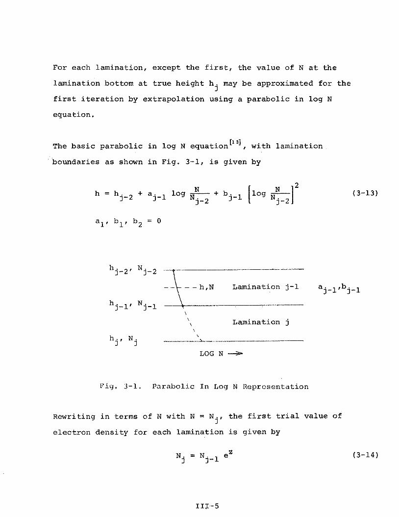
For each laminat ion, except t h e f i r s t , t h e va lue of N a t t h e
laminat ion bottom a t t r u e he igh t h may be approximated f o r t h e j
f i r s t i t e r a t i o n by e x t r a p o l a t i o n using a pa rabo l i c i n log N
equation.
The b a s i c pa rabo l i c i n log N equation[13], wi th laminat ion
boundaries a s shown i n Fig. 3-1, is given by
N M 2 h = hje2 + ajml 109 --- + bj-l log -
N j - 2 Nj-2
hj-2, N j - 2 __-l_l_.-- -----
- I-- .- h , N Lamination j-1 a j -1 , b j-1
\ \ Lamination j \
h N \
j f j --..- "2%" --.-- ---- LOG N +
r i g . 3 - 1 . Parabol ic I n Log N ~ e p r e s e n t a t i o n
Rewriting i n terms of N with N = N t h e f i r s t t r i a l va lue of j *
e l e c t r o n dens i ty f o r each laminat ion is given by
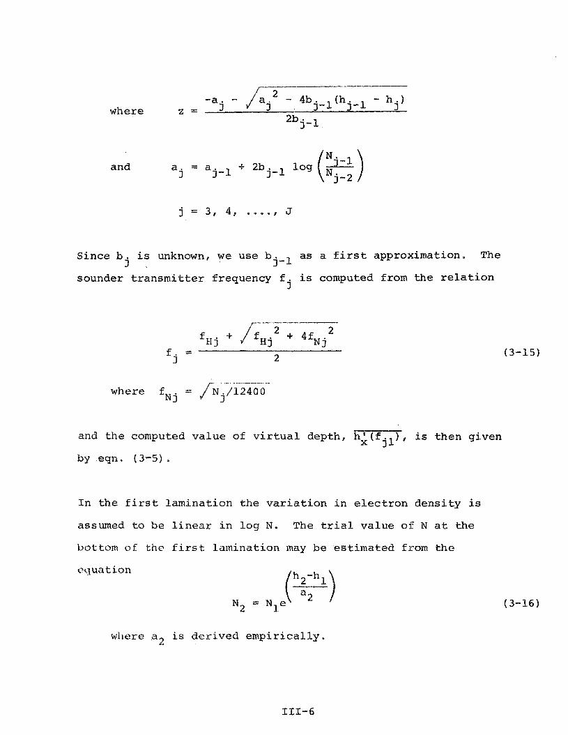
a - /aj' - j 4bj-l(hj- l - h j ) where z =
2bj-l
and a = j
S ince b is unknown, w e use bjml a s a f i r s t approximation. The j .
sounder t r a n s m i t t e r frequency f i s computed from t h e r e l a t i o n j
- . . . - - - . - where f = f ~ ~ / 1 2 4 0 0
N j
and t h e computed v a l u e of v i r t u a l dep th , h j is t h e n given
by eqn. ( 3 - 5 ) ,
I n t h e f i r s t l amina t ion t h e v a r i a t i o n i n e l e c t r o n d e n s i t y is
assumed t o be l i n e a r i n log N. The t r i a l va lue o f N a t t h e
bottom of thc first l amina t ion may be e s t i m a t e d f r o m t h e
equation
wliere a2 is d e r i v e d e m p i r i c a l l y .
An a l t e r n a t i v e method of e s t a b l i s h i n g i n i t i a l va lues o f N a t j
each l amina t ion boundary was d e s c r i b e d i n S e c t i o n I11 o f t h e
Study Report , P a r t 1[16]. I n t h i s method, v a l u e s o f N are j
Linear ly e x t r a p o l a t e d from t h e two prev ious ionograms i n t h e
same pas s a t c o n s t a n t l amina t ion boundary l e v e l s . The
e x t r a p o l a t i o n method should work f o r a l a r g e c l a s s o f ionograms
where t h e g r a d i e n t s a t c o n s t a n t t r u e h e i g h t
h .=cons t a n t 3
vary s lowly th roughout t h e pas s .
If h;(f. ) < hA(f 1 , as i n F ig . 3-2, t h e t r i a l va lue o f N was 11 j l j l
too l a r g e . For t h e second i t e r a t i o n choose
where a - . O 1 w i t h t h e s i g n - f o r < h'
and + f o r hC > h '
The second s u b s c r i p t i n t h e above n o t a t i o n i s t h e i t e r a t i o n count .
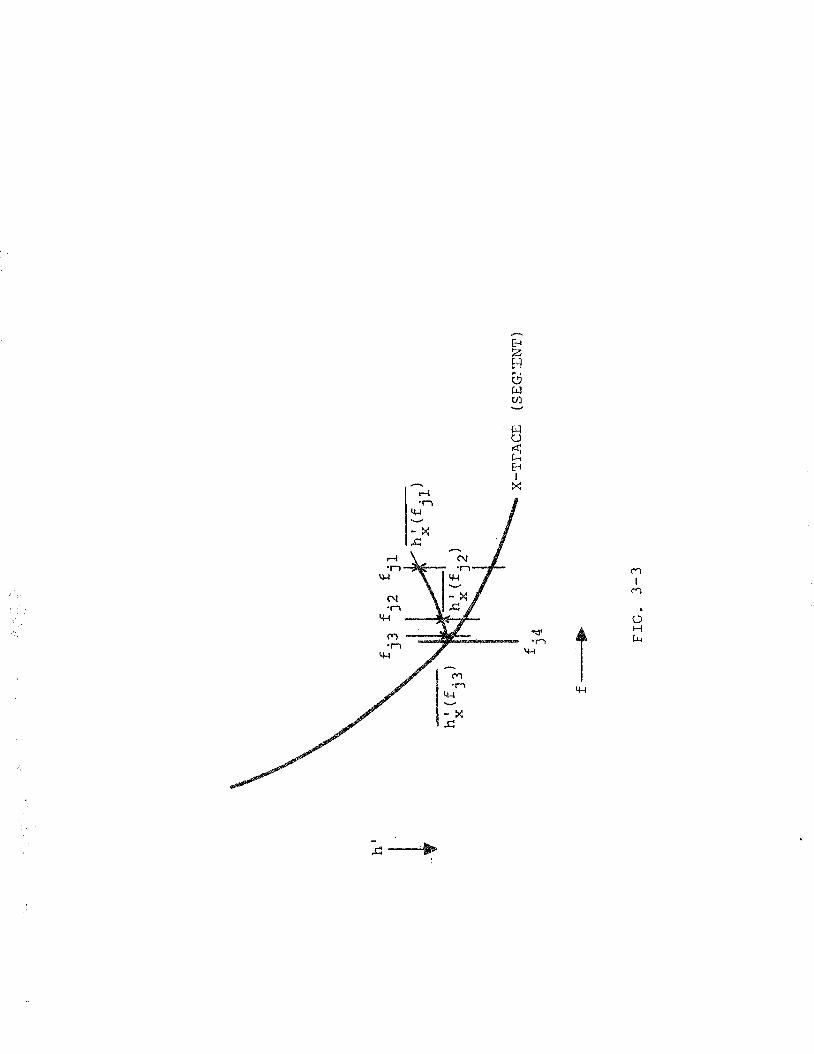
If h;(f. ) > h;(f ) , t h e t r i a l v a l u e o f N was t o o sma l l . A I 2 j 2 j 2
s t r a i g h t l i n e t h r u p o i n t s h k ( f ) and hi(£ ) w i l l i n t e r s e c t t h e j l j 2
X-Trace at f j 3 , a s shown i n Fig . 3-2 where the f i r s t t w o p o i n t s
a r e on o p p o s i t e sides o f t h e X-Trace, o r i n F ig , 3-3 where t h e
f i r s t t w o p o i n t s f a l l on t h e same s i d e of t h e X-Trace.
CV 'PI
%I
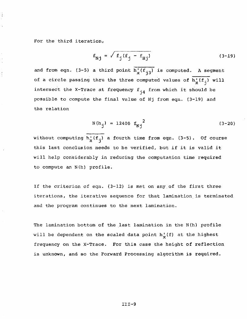
For the third iterationr
and from eqn. (3-5) a third point h;(f. ) is computed. A segment 13
of a circle passing thsu the three computed values of h'(f.) will x I
intersect the X-Trace at frequency f from which it should be j 4
possible to compute the final value of Nj from eqn. (3-19) and
the relation
without computing hs (f ,) a fourth time from eqn. (3-5). Of course x 1
this last conclusion needs to be verified, but if it is valid it
will help considerably in reducing the computation time required
to compute an N(h) profile.
If the criterion of eqn. (3-12) is met on any of the first three
iterations, the iterative sequence for that lamination is terminated
and the program continues to the next lamination.
The lamination bottom of the last lamination in "c'ne N(h) profile
will be dependent on the scaled data point h;(f) at the highest
frequency on the X-Trace, For this case the height of reflection
is unknown, and so the Foxward Processing algorithm is required.
The objectives of the Inverse Processing nethod are as follows:
a* Hinimize the computer time required to compute an
IPJ (k) profile.
. Simplify the implementation of mixed-mode proce~sing.
c, Optimize the spacing between lamination bound4ries of
the N ( h ) profile.
d. Make the lamination boundaries the same for all
ionograms for convenience in interpolating and
extrapolating values of N (h) , fH and 4 .
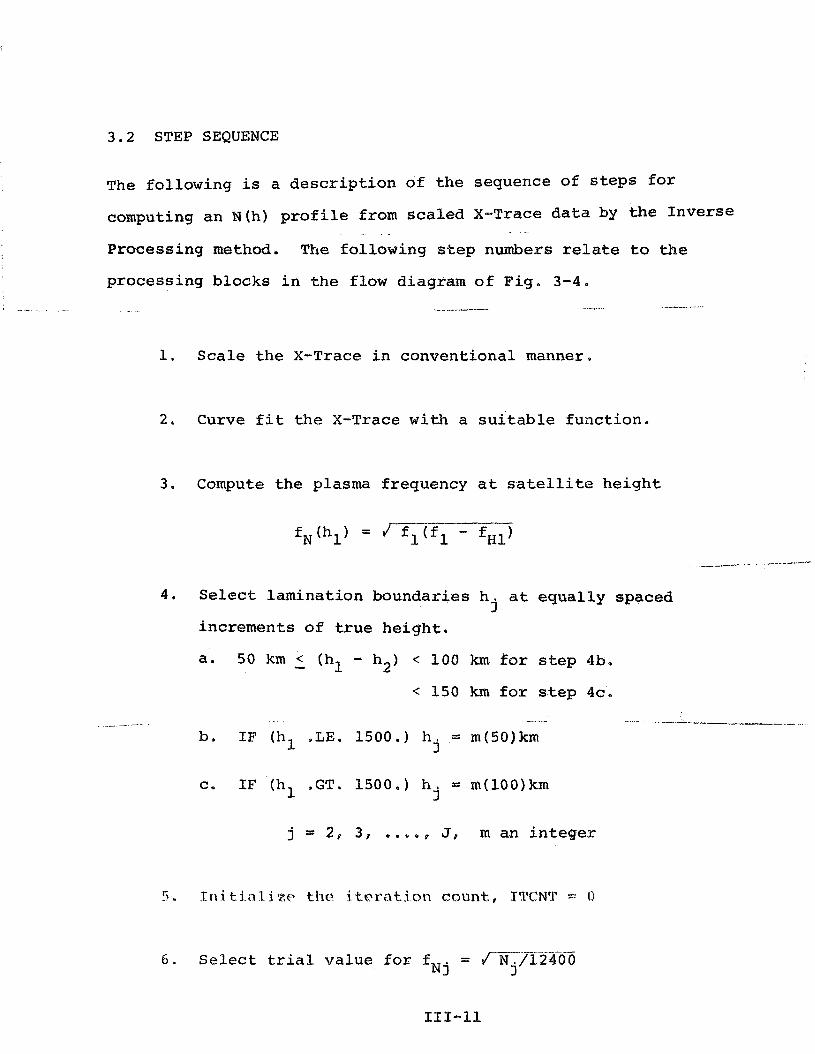
3.2 STEP SEQUENCE
The following is a description of the sequence of steps for
computing an N(h) profile from scaled X-Trace data by the Inverse
Processing methad. The following step numbers relate to the
processing blocks in the flow diagram of Fig. 3 - 4 -
I _ ----. - - --- -- --
1. Scale the X-Trace in conventional manner.
2. Curve fit the X-Trace with a suitable function.
3. Corr,pute the plasma frequency at satellite height
4, Select lamination boundaries h at equally spaced j
increments of true height,
a. 50 km - < (hl - ha) < 100 km for step 4b.
< 150 km for step 4c.
J z% 2 @ 3, . . . . p J I m an integer
5 . I n i t i n 1 i zc t l ic? i trrnt jcsn c o u n t , lTCNt1' = 0
6. Select trial value for f = -712403 N j
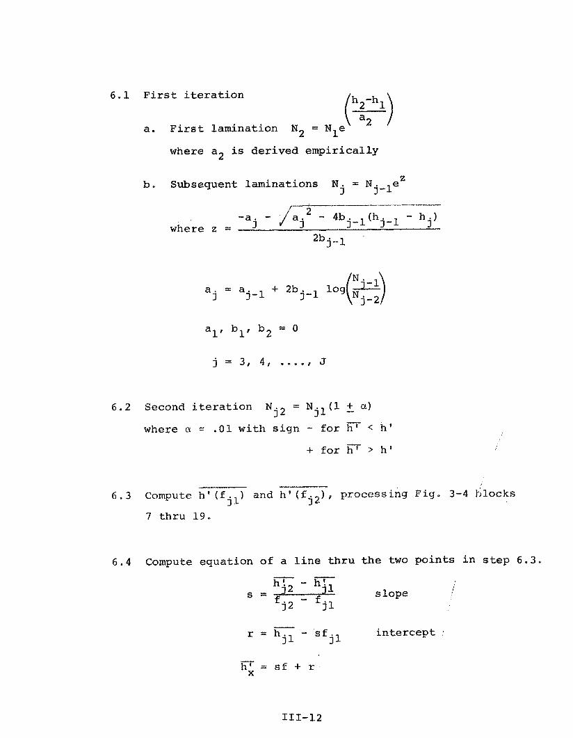
6 . 1 F i r s t i t e r a t i o n
a. F i r s t l amina t ion N2 = N l e \ a 2 /
where a 2 i s d e r i v e d e m p i r i c a l l y
b. Subsequent l amina t ions N = N j - l e z j
-a - /aj ' - j 4bj- l (hj - l
- hj) where z =
2b j-l
6.2 Second i t e r a t i o n N = N (1 + a ) 12 j 1
where a = . 01 w i t h s i g n - f o r h' < h i
-I- f o r h'> h i
- 6 . 3 Compute h v ( f ) and h q ( f . ) , proces s ing F ig . 3-4 i ; locks
I 2 7 t h r u 1 9 .
6.4 Compute equa t ion o f a l i n e t h r u t h e two p o i n t s i n s t e p 6 . 3 . - - h!* - h!l
s = I
s l o p e , f j 2 - f j l
- r = h - s f
jl jl i n t e r c e p t :
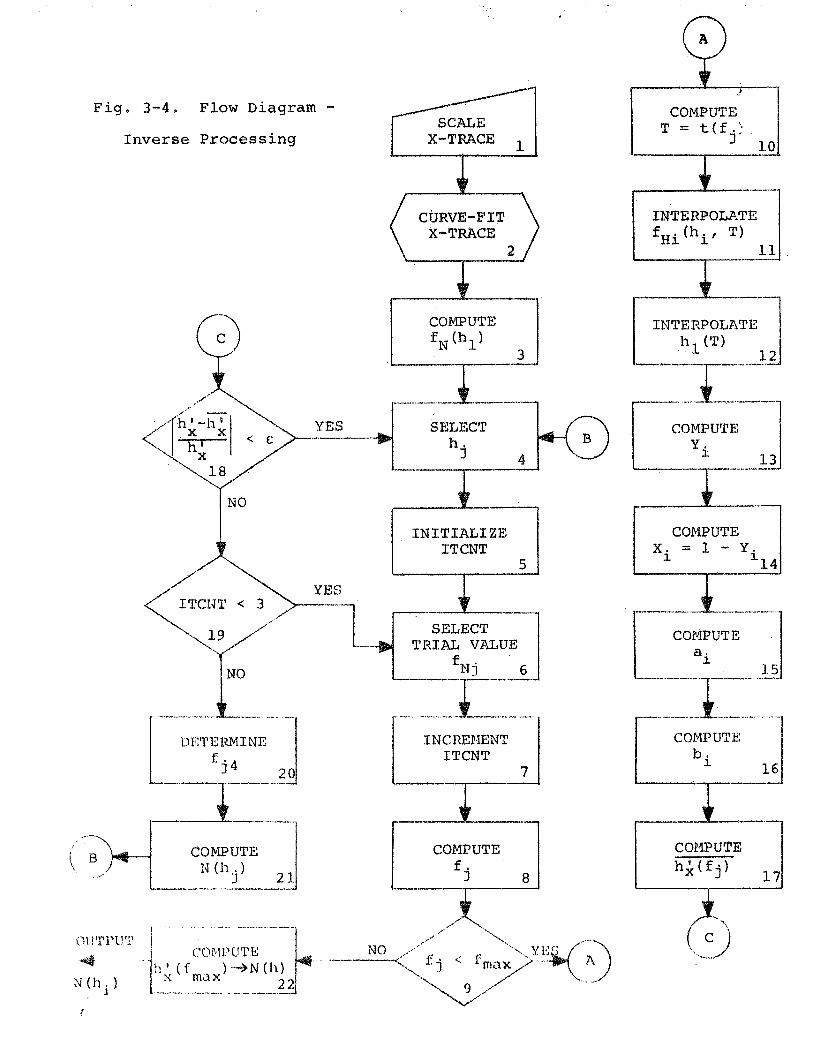
Fig. 3-4. Flow Diagram - SCALE /
Inverse Processing
INITIALIZE
TRIAL VALUE
INCREPlENT
I INTERPOLATE I
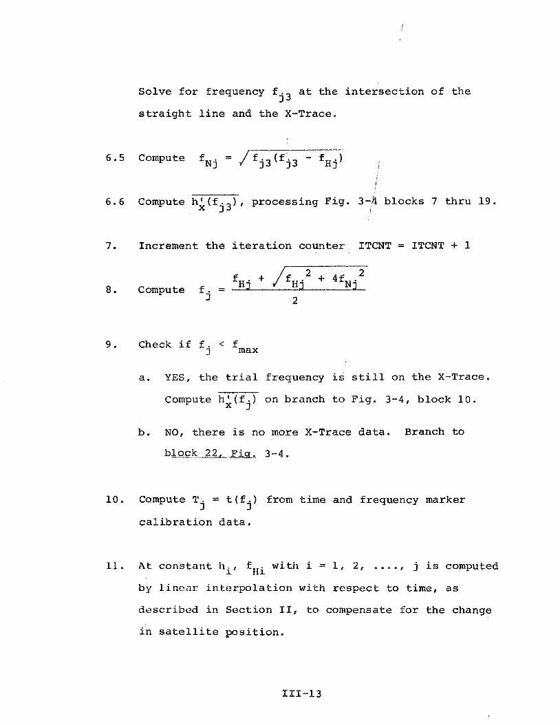
Solve f o r f requency f a t t h e i n t e r s e c t i o n o f t h e j 3
s t r a i g h t l i n e and t h e X-Trace.
----- 6.5 Compute f N j = J f j3 ( f j3 - f H j )
I
6 . 6 Compute h; (f ) , proces s ing Fig . 3-kl b locks 7 t h r u 19. j 3 I
7. Increment t h e i t e r a t i o n coun te r ITCNT = ITCNT + 1
9. Check i f f j < fmax
a. YES, t h e t r i a l frequency i s s t i l l on t h e X-Trace.
Compute h ; ( f . ) on branch t o F ig . 3-4 , block 10. 3
b. NO, t h e r e is no more X-Trace d a t a . Branch t o
brp_ck._22--... 3-4 *
10. Compute T = t ( f . ) from t i m e and f requency marker j J
c a l i b r a t i o n d a t a .
11. A t c o n s t a n t hi, fIii w i t h i * 1, 2 , ...., j i s computed
by l i n e a r i n t e r p o l a t i o n wi th r e s p e c t t o t i m e , as
d e s c r i b e d i n S e c t i o n II, to compensate f o r t h e change
i n s a t e l l i t e p s i t i o n .
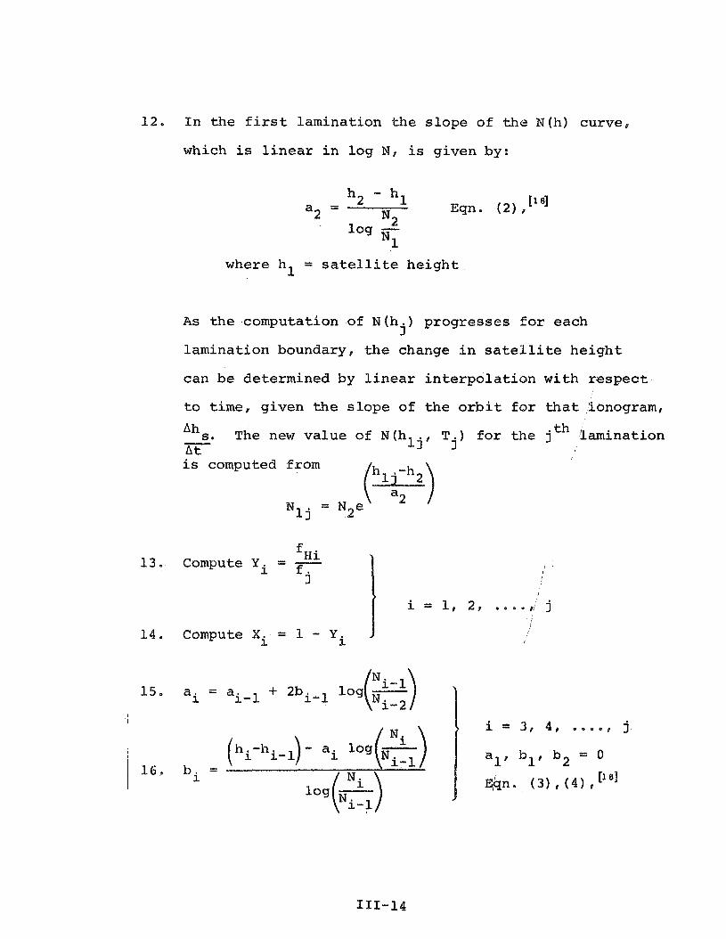
1 2 . I n t h e f i r s t lamination t h e s lope of t h e N(h) curve,
which i s l i n e a r i n log N, i s given by:
L log - N,
where hl = s a t e l l i t e h e i g h t
A s t h e computation of N (h . ) progresses f o r each I
laminat ion boundary, the change i n s a t e l l i t e h e i g h t
can be determined by l i n e a r i n t e r p o l a t i o n with m s p e c t
t o t ime, given the s l o p e of t h e o r b i t f o r t h a t Lonogram,
Ahs. - The new value of N(hlj , T . ) f o r t h e jth lamination At 3 i s computed from
I
M = N2e l j
L H i 13. Compute Yi = - f j
1
i = l r 28 e o a * ,/' j
1 4 . Compute Xi = 1 - 'i I
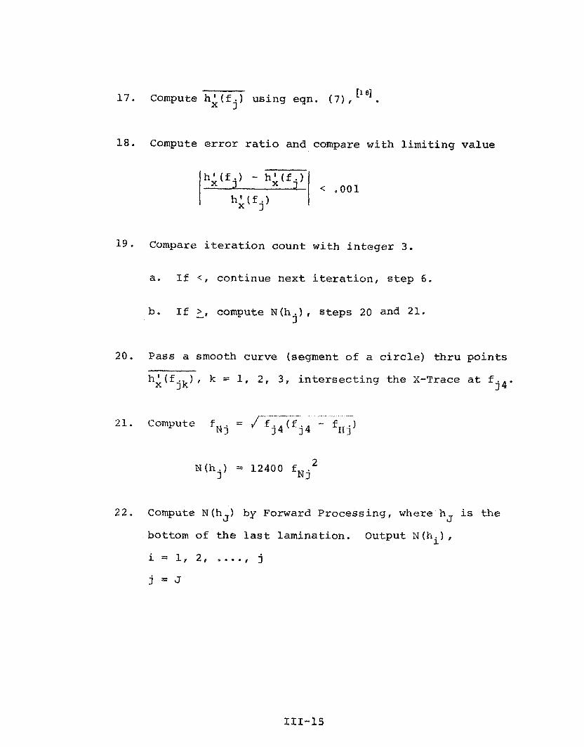
17. Compute h;(f.) us ing eqn. ( 7 ) , [181
3
18. Compute error r a t i o and compare wi th l i m i t i n g value
1 9 , Compare i t e r a t i o n count with i n t e g e r 3 .
a. I f <, con t inue n e x t i t e r a t i o n , s t e p 6.
b e I f L~ compute N (h . ) , s t e p s 20 and 21. 3
20. Pass a smooth curve (segment of a circle) t h r u points
hi (f jk) , k = 1, 2 , 3 , i n t e r s e c t i n g t h e X-Trace a t f j4 .
= /-;:-( --f-. , - . . .- 21. Compute f
N j 3 4 j4 - '11j'
2 2 . Compute N ( h J ) by Forward P roces s ing , where hJ i s the
bottom of t h e last l amina t ion . Output bJ(hi) . i = 1, 2 1 ...., j
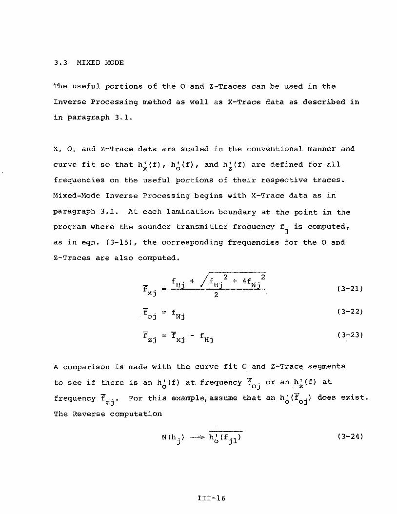
3 . 3 MIXED MODE
The u s e f u l p o r t i o n s o f t h e 0 and Z-Traces can be used i n t h e
Inve r se P roces s ing method as w e l l as X-Trace d a t a a s described i n
i n paragraph 3-1.
X , 0, and Z-Trace d a t a a r e s c a l e d i n t h e convent iona l manner and
cu rve fit s o t h a t h i ( f ) , h A ( f ) . and ha ( f ) are de f ined f o r a l l
f r equenc ie s on t h e u s e f u l p o r t i o n s o f t h e i r r e s p e c t i v e t r a c e s .
Mixed-Mode I n v e r s e P roces s ing beg ins w i t h X-Trace d a t a a s i n
paragraph 3.1. A t e ach l a m i n a t i o n boundary a t t h e p o i n t i n t h e
program where t h e sounder t r a n s m i t t e r f requency f is computed, j
as i n eqn, (3-15) , t h e cor responding f r e q u e n c i e s f o r t h e 0 and
Z-Traces a r e a l s o computed.
A comparison i s made with t h e curve f i t 0 and Z-Trace, segments
t o s e e i f t h e r e i s an hA(f ) a t f requency i o r a n h i ( £ ) a t 0 j
frequency iz j. For t h i s example,assurne t h a t a n ) does e x i s t .
The Reverse computation
gives t h e f i r s t p o i n t f o r laminat ion j on t h e h ( 2 ) plane , he
i t e r a t i v e sequence cont inues as i n paragraph 3.1, except f o r t h e
t h i r d i t e r a t i o n where
from which a t h i r d p o i n t hA( f . ) is computed. A segment of a 33
c i r c l e pass ing t h r u t h e t h r e e computed va lues of h: ( f . ) w i l l 3
i n t e r s e c t t h e 0-Trace a t frequency f j d r from which it should be
p o s s i b l e t o compute t h e f i n a l value of N from eqn. (3-25) and j
eqn. (3-20).
To compute N (h .) with r e s p e c t t o curve f i t Z-Trace d a t a use eqn. 3
(3-23) and the Reverse computation
A t any laminat ion boundary h it would be poss ib le t o compute an j '
N (h . ) with respec t t o each of t h e X, 0, o r Z-Traces , assuming t h e 3
t r a c e s have been s c a l e d a t t h e r e l a t e d sounder pu l se frequencies .
The value of N(h . ) would be s l i g h t l y d i f f e r e n t f o r each t r a c e 3
and would depend of course on t he delay contribution of t h e
previous laminat ions.
O n t h e b a s i s t h a t t h e 0-Trace is usual ly th inner than e i t h e r t h e
X or 2-Trace, t h e program l o g i c f o r Mixed Mode Invers,e Processing
might be t o compute N (h . ) wi th r e s p e c t t o t h e 0-Trace whenever 3
poss ib le , otherwise use X-Trace da ta . When processing with

r e spec t t o t h e 0-Trace, corresponding h i (f .) po in t s could be 3
computed t o a s s i s t i n de f in ing t h e v e r t i c a l r e f l e c t i o n por t ion
of a d i f f i c u l t X-Trace. . .
SECTION I V
MATRIX PROCESSING
4.0 INTRODUCTION
One of t h e problems an opera to r f aces when processing ionograms
with t h e FILMCLIP System occurs a f t e r one process ing i t e r a t i o n
represented by
I f t h e computed 0-Trace d a t a p o i n t s h A ( f . ) d o n ' t match c l o s e l y 3
enough t h e i d e n t i f i a b l e 0-Trace on t h e i o n o g r m , t h e opera to r
must change some of t h e sca led d a t a po in t s on t h e X-Trace i n an
e f f o r t t o modify t h e N ( h ) p r o f i l e s o t h a t t h e computed hA(f . ) 3
d a t a p o i n t s w i l l match t h e 0-Trace more c l o s e l y . T h i s i s r e a l l y
a very complex, multi-dimensional, non-linear problem t h a t a
human being is n o t equipped t o handle, except by t r i a l and e r r o r .
With the FILMCLIP System an opera to r can make adjustments i n the
p o s i t i o n s of t h e s c a l e d d a t a p o i n t s on t h e X-Trace and observe
t h e r e s u l t s r e f e r r e d t o t h e 0-Trace i n success ive i t e r a t i o n s
u n t i l a s u i t a b l e match i s achieved, With experience, ope ra to r s
become q u i t e s k i l l e d i n making adjustments i n t h i s i t e r a t i v e
loop, bu t i t s t i l l remains a t i m e consuming and i n e f f i c i e n t
procedure,
The matr ix method provides a l o g i c a l means whereby t h e computer
can use a l l t h e normally a v a i l a b l e information i n an ionogram
t o compute an N (h) p r o f i l e i n a weighted l e a s t squares sense.
The computation t ime t o compute an M(h) p r o f i l e by t h e matr ix
method w i l l i nc rease s u b s t a n t i a l l y over t h e t i m e requi red f o r
e i t h e r t h e Forward o r Inverse methods, However, it w i l l t ake
t h e o p e r a t o r o u t of t h e i t e r a t i v e loop f o r closed-loop
processing s o t h a t t h e r e may be an o v e r a l l reduct ion i n elapsed
time. I n a d d i t i o n , t h e matr ix method o f f e r s some unique advantages
not a v a i l a b l e i n o t h e r methods.
T h e matr ix method of ionogram d a t a reduct ion uses an a n a l y t i c
model of t h e N ( I a ) p r o f i l e r a t h e r than t h e laminat ion model of
~ a c k s o n " ~ ] . The concept behind matr ix processing i s to set up
a mathematical model of t h e N (h) p r o f i l e and then a d j u s t t h e
c o e f f i c i e n t s of t h e mathematical model t o minimize the e r r o r
between s c a l e d and computed values of h f (fi) i n a weighted l e a s t
squares sense ,
A sct of sca lcd 11' (fi) data po in t s from an ionograrn is t h e inpu t
prescr i .y t ion vec tor t o the matr ix program. The d a t a po in t s can
bc scaled from Loth t h e X and 0-Traces and even the 2-Trace when
i.t is a v a i l a b l e . A weighting c o e f f i c i e n t i s assigned t o each
d a t a po in t using an a r b i t r a r y s c a l e from 1 t o 10. Good d a t a
p o i n t s a r e weighted h igher than ques t ionable d a t a po in t s so t h a t
t h e r e s u l t a n t N(h) p r o f i l e is inf luenced more by t h e d a t a p o i n t s
i n which t h e opera to r has g r e a t e r confidence and t o a l e s s e r
e x t e n t by d a t a p o i n t s with a lower weighting f a c t o r .
The p a r t i c u l a r model used f o r mat r ix process ing i s a r a t i o of
polynomials o f t h e type used i n syn thes iz ing e l e c t r i c a l f i l t@'k
t r a n s f e r func t ions , It i s perhaps one of those f o r t u i t o u s
circumstances, bu t when a s e t o f N(h) va lues were inpu t t o a
s l i g h t l y modified Astrodata p r o p r i e t a r y program f o r f i l t e r
syn thes i s , a curve f i t w i th in 1% was achieved t h e f i r s t t ime t h e
s i g h t number of poles and zeros w e r e s p e c i f i e d .
With t h e matr ix method i t i s d e s i r a b l e t o minimize t h e number o f
coeff ic ' ients requi red t o model t h e M(h) p r o f i l e , because some
matr ix opera t ions on t h e computer go up a s m3 where m i s t h e o rde r
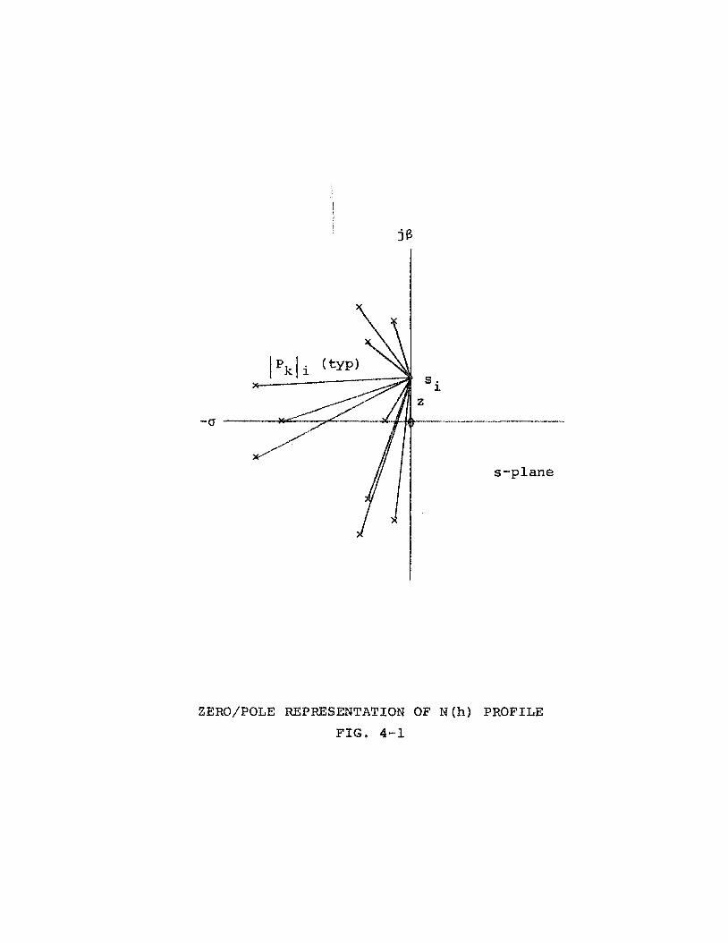
of a square matr ix . The r o o t s of t h e numerator and denominator can
be p l o t t e d as po les and zeros i n t h e complex s-plane. A p l o t of
t h e poles and zeros f o r one model i s shown i n Fig. 4-1. I n t h i s
model t h e r e a r e four conjugate complex po les* two r e a l poles , and
one zero a t the o r i g i n , O the r models i n v e s t i g a t e d have used f i v e
sr s i x complex poles with from two t o f i v e zeros a t t h e o r i g i n and
no r e a l poles . The number of a d j u s t a b l e c o e f f i c i e n t s r equ i red f o r
t h e s e models v a r i e s from 10 t o 1 2 . Kinkel [ ' proposed a model
w i t h 5 v a r i a b l e s which turned o u t t o be an i n s u f f i c i e n t number.

The choice of t h e p a r t i c u l a r zero/pole r e p r e s e n t a t i o n f o r an
N(h) p r o f i l e depends on a number of f a c t o r s , such as t h e r a t i o
of,minimum to maximum e l e c t r o n d e n s i t y and t h e shape of t h e curve. i
A b i t t l e experience i n c u r v e - f i t t i n g a v a t i e t y of ~ ( h ) p r o f i l e s , i
us/ing Program NHMODEL i n Sect ion 4 . 4 , w i l l provide t h e , b a s i s
f 4 r s e l e c t i n g t h e i n i t i a l va lues f o r c o e f f i c i e n t s of t h e model
used i n t h e matr ix method.
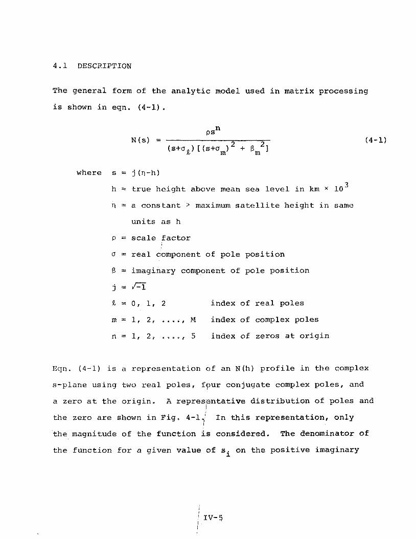
4.1 DESCRIPTION
The general form of the analytic model used in matrix processing
is shown in eqn. (4-1)
where s = j (0-h)
h = true height above mean sea level in km x 10 3
7'1 = a constant > maximum satellite height in same
units as h
P = scale factor
0 = real aomponent of pole position
B = imaginary component of pole position
j = f i
R = 0, 1, 2 index of real poles
m = 1, 2, ...., M index of complex poles
n = 1, 2, ..,., 5 index of zeros at origin
Kiln. (4-1) is n representation of an N(h) profile in the complex
s-plane usiny two real poles, four conjugate complex poles, and
a zero at the origin. A representative distribution of poles and 1
the zero are shown in Fig, 4-1.: In this representation, only I
the magnitude of the function is considered. The denominator of
the function for a given value of si on the positive imaginary
s-plane
ZERO/POLE REPRESENTATION OF N (h ) PROFILE
F I G . 4 - 1
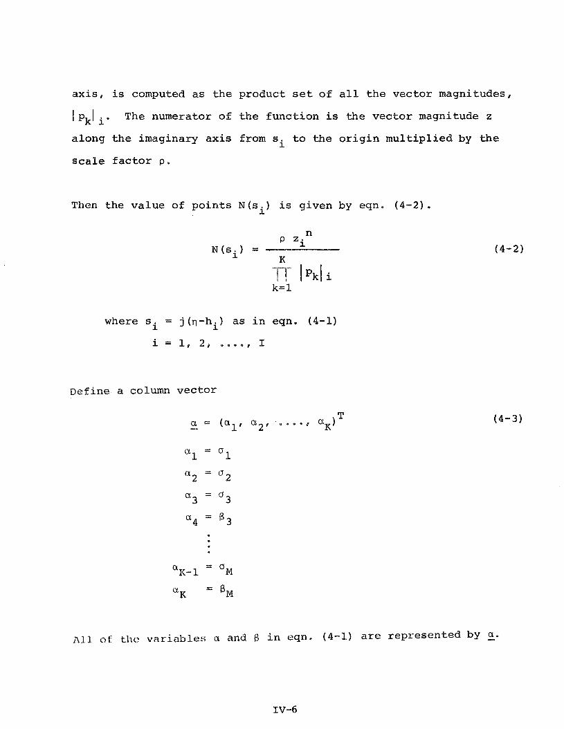
a x i s , is computed as t h e produc t set o f a l l t h e v e c t o r magnitudes,
I pkl i - The numerator o f t h e f u n c t i o n is t h e v e c t o r magnitude z
a long t h e imaginary a x i s from s t o t h e o r i g i n m u l t i p l i e d by t h e i
s c a l e f a c t o r p .
Then t h e v a l u e of p o i n t s N ( s i ) i s g iven by eqn. (4-2).
where si = j (q-hi) a s i n eqn. (4-1)
i = l I 2,a e e e e , I
Define a column v e c t o r
A l l of thc vnri .ables a and 6 i n eqn. ( 4 - 1 ) are r ep re sen ted by - a,
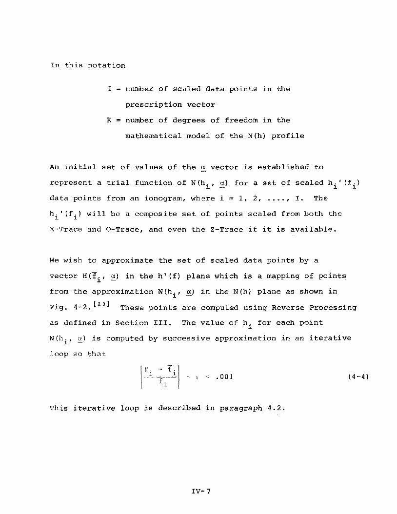
I n t h i s n o t a t i o n
I = number o f s c a l e d d a t a p o i n t s i n t h e
p r e s c r i p t i o n v e c t o r
K = number of degrees of freedom i n t h e
mathemat ical modei of t h e N(h) p r o f i l e
An i n i t i a l se t o f v a l u e s o f t h e - a v e c t o r is e s t a b l i s h e d t o
r e p r e s e n t a t r i a l f u n c t i o n o f N (hi. - a ) f o r a s e t o f s c a l e d h i ' ( f i )
d a t a p o i n t s from an ionogram, wh'zre i = 1, 2 , . ... , I. The
h i 1 (.ti) w i l l bc a composite s e t o f p o i n t s s c a l e d from bo th t h e
X-Trace and 0-Trace, and even t h e 2-Trace i f it is a v a i l a b l e .
W e wish t o approximate t h e se t o f s c a l e d d a t a p o i n t s by a
v e c t o r H (fit - a ) i n t h e h v ( f ) p l a n e which i s a mapping o f p o i n t s
from the approximat ion N(hi, - a ) i n t h e N(h) p l a n e as shown i n
F ig . 4-2. 1 2 ' ] These p o i n t s are computed u s i n g Reverse Process ing
a s de f ined i n S e c t i o n 111. The v a l u e of hi f o r each p o i n t
N ( h i , 2) i s computed by s u c c e s s i v e approximation i n an i t e r a t i v e
Th i s i t e r a t i v e l oop i s d e s c r i b e d i n paragraph 4 . 2 .
h t - ( f ) p l a n e M(h) p l a n e
F ig . 4-2, Mapping o f Corresponding P o i n t s i n
t h e h ' (f) and N (h ) P l anes
The d i f f e r e n t i a l of t h e func t ion H (Ti, 2) can be approximated
by a s m a l l increment on each ak a s i n eqn. (4-5) .
Eqn. (4-3) expressed i n g r a d i e n t n o t a t i o n becomes
AH (Ti, - a) = v ,H(F~ ' 2) An - -
- (Ti 2) a 1 4 ( f i J - a) where VaH(fi, 2) = I . . e m f - a a~

W e wish t o f i n d
Rearranging terms and normal iz ing by d i v i d i n g both s i d e s by
EUfiP - a)
Combining eqn. (4-6) and eqn. ( 4 -8 ) and expanding i n m a t r i x form
g i v e s
For i = 1,
h ' ( f l ) = 0
where - fl - f x s
Consequently % and alk, k = 1' 2 , ...., K, must be r e d e f i n e d i n
terms of f requency because AH has no meaning a t s a t e l l i t e h e i g h t .
For t h i s case
I n compact m a t r i x n o t a t i o n
I n eqn. (4-9 ) t h e r e are I equa t ions w i t h K unknowns. With
I > K t h e r e are more equa t ions t han unknowns s i n c e t y p i c a l l y
20 < 1 5 30 - and 10 - < K - < 12
A least squa re s f i t s o l u t i o n [I9' can b e o b t a i n e d by f i r s t
mu l t i p ly ing bo th s i d e s of eqn. (4-10) by AT, which g i v e s
where T t h e t r a n s p o s e
Then a l e a s t squares e s t i m a t e of t h e adjustment vec to r A% i s
given by
We wish t o ass ign a weighting c o e f f i c i e n t , w iiP t o each s c a l e d
h q ( f i ) d a t a po in t i n o rde r t h a t good d a t a po in t s e x e r t a g r e a t e r
inf luence on the l e a s t squares approximation of N (h , - a) than
ques t ionable d a t a po in t s . Define a diagonal matr ix of weights
a s follows:
The weight ing matr ix W - i s incorpora ted i n t h e l e a s t squares f i t n
s o l u t i o n of Aa - t o g ive a weighted l e a s t squares adjustment vec tor
as follows:

For each i t e r a t i o n then
where n = i t e r a t i o n count
which g ives a new s e t of c o e f f i c i e n t s f o r t h e a n a l y t i c model
N(h, E) . The i t e r a t i v e cyc2e cont inues u n t i l .r+i
* '
A more d i r e c t measure of how w e l l t h e computed d a t a p o i n t s
B (Fit a) match the s c a l e d d a t a p o i n t s h ' ( f i ) might be obta ined
by de f in ing a c o s t func t iona l J a s the sum s e t of t h e weighted,
normali zed e r r o r squared.
where
The i t e r a t i v e c y c l e would then cont inue u n t i l
n = i terati011 count
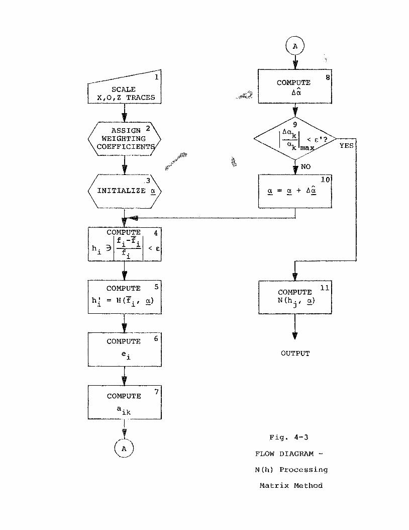
A flow diagram showing t h e major processing s t e p s i n a program
f o r t h e matr ix method i s shokn i n Fig. 4 - 3 .
4.2 STEP SEQUENCE
The following is a description of the uence of steps for
computing an N(h) profile from scaled X-Trace data by the Matrix
Processing method. The following step numbera relate to the
processing blocks in the flow diagram of F'ig. 4-3 .
1. Scale the X, 0, and 2-Traces of an ionogram in
conventional manner.
2. ~ssign a weighting coefficient to each scaled
data point.
3. Establish initial values of coefficients for a. - Program NHMODEL has been developed for doing this
and is described in paragraph 4.4.
4. Compute values of hi corresponding to frequencies fi
of scaled data points hl(fi) such that
This is accomplished by a one-dimensional search f Z 3 ]
using successive approximations and is described in
pi~ra(]r~ipI~ 4 . 3 * This makes possible comparison of
c-cjn~putctf , ~ ~ l c l :;cal.ccl data points at tlie same frequency
i n t i l c ~ I1 ' ( I - ) -planc.
IV- 13
SCALE
WEIGHTING COEFFICIENT
COMPUTE 8
&+&.,2 A$
OUTPUT
Fig. 4-3
FLOW DIAGRAM - N (h) Processing
Matrix Method
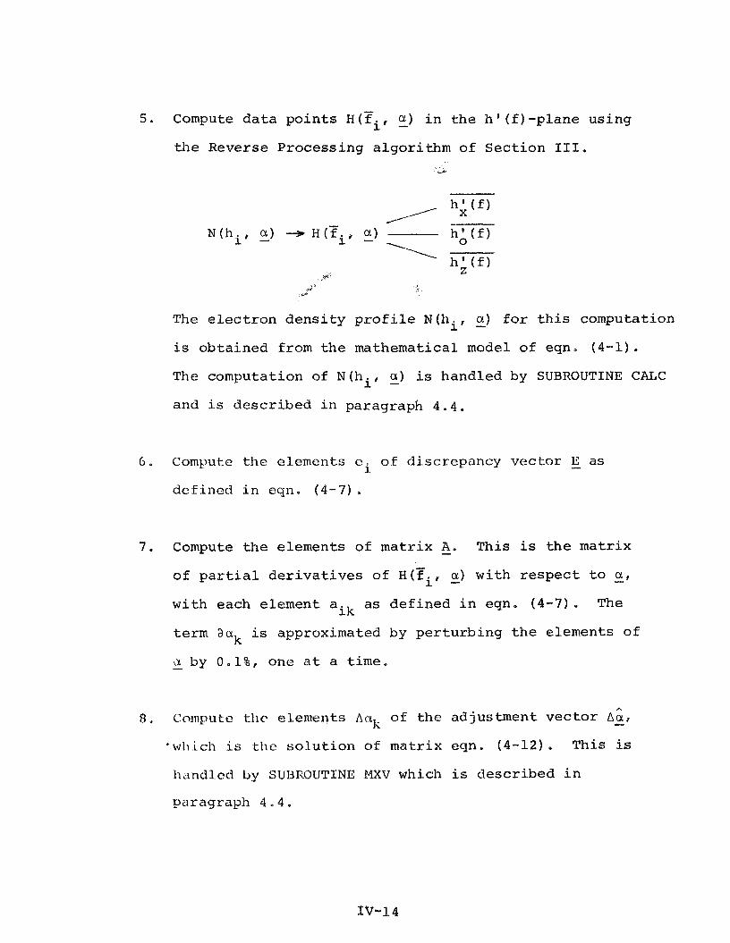
5. Compute d a t a po in t s H (Ti. - a) i n t h e h v ( f ) -plane using
t h e Reverse Processing a lgor i thm of Sec t ion 111.
7'
u"
The e l e c t r o n d e n s i t y p r o f i l e N(hi, - a ) f o r t h i s computation
is obtained from t h e mathematical model of eqn. ( 4 - 1 ) .
The computation of N(hi, - a ) is handled by SUBROUTINE CALC
and is descr ibed i n paragraph 4 . 4 .
6 . Compute t h e elements e of discrepancy vec tor I2 as i -
def ined i n egn. (4-7) .
7 . Compute t h e elements of mat r ix A, - This is t h e matr ix
of p a r t i a l d e r i v a t i v e s of H ( V ~ , - a) wi th r e s p e c t t o - a .
with each element aik a s def ined i n eqn. (4-7) . The
term ask is approximated by pe r tu rb ing t h e elements of
a by 0.1%, one a t a t ime, -
8. Compute tllr e lements Aixk of t h e adjustment vec to r A;, - 'wl~ich j.s the s o l u t i o n of mat r ix eqn. ( 4 - 1 2 ) . This is
h , ~ n d l c d by SUBROUTINE MXV which i s descr ibed i n
paragraph 4 . 4 .
9 . This s t e p is a d e c i s i o n block t o determine whether o r
n o t t h e l a t e s t adjustment v e c t o r w i l l make a s i g n i f i c a n t
change i n t h e c o e f f i c i e n t s of t h e mathematical model
of t h e N(h) p r o f i l e . If t h e maximum abso lu te va lue o f
a l l t h e change r a t i o s o f v e c t o r - a a r e less than E ,
w r i t t e n a s ,*'
b
a . NO, branch t o S t e p 10. Repeat steps 4 t h r u 9 ,
b. YES, a weighted l e a s t squares s o l u t i o n f o r N (hi , - a )
has been obta ined .
10, Add t h e adjustment v e c t d r Aa - t o t h e s t a t e v a r i a b l e s - a an?
r e p e a t s t e p s 4 t h r u 9 .
11. Output N(h j r - a ) a t equa l ly spaced increments of t r u e
height h I
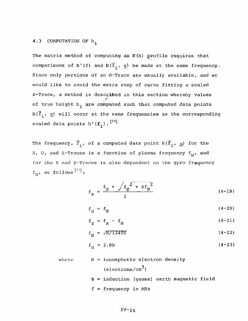
The m a t r i x method of computing an Nlh) p r o f i l e r e q u i r e s t h a t -"*
comparisons o f h 9 ( f ) and H (Fit - a ) b e made a t t h e same frequency.
S ince on ly p o r t i o n s of an O-Trace a r e u s u a l l y a v a i l a b l e , and w e
would l i k e t o avoid t h e e x t r a s t e p of curve f i t t i n g a s c a l e d
X-Trace, a method is described i n t h i s s e c t i o n whereby va lues 4.
of t r u e h e i g h t hi a r e computed svch t h a t computed d a t a p o i n t s
~ ( 7 ~ ~ 2) w i l l o ccu r a t t h e same f r equenc ie s a s t h e cor responding
s c a l e d d a t a p o i n t s h ' ( f i ) . l2 3~
- he f requency, f i , o f a computed d a t a p o i n t H (zit - a ) for the
X , 0, and Z-Traces is a f u n c t i o n o f plasma frequency f N , and
f o r the X a n d Z-Traces i s a l s o dependent o n the gyro frequency
* fH' as fo l lows a
N = ionospheric e l e c t r o n d e n s i t y
3 (e lcc t sons /cm )
B = i n d u c t i o n (gauss ) e a r t h magnetic f i e l d
f = frequency i n MHz
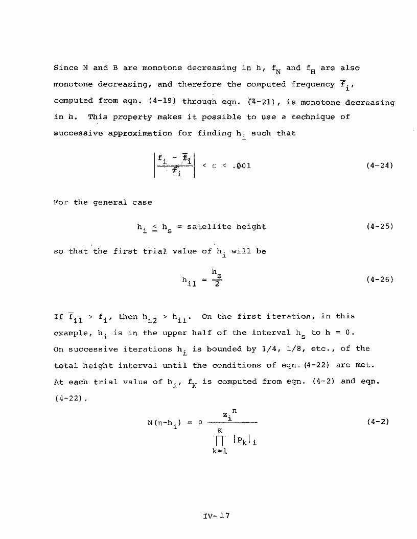
Since N and B a r e monotone dec reas ing i n h , f N and f H a r e a l s o
monotone dec reas ing , and t h e r e f o r e t h e computed frequency Tip
computed from eqn- (4-19) through eqn. ('4-21), i s monotone d e c r e a s i n g
i n h. This p rope r ty makes it p o s s i b l e t o u s e a t echnique of
s u c c e s s i v e approximation f o r f i n d i n g hi such t h a t
For t h e g e n e r a l c a s e
hi - < hs = s a t e l l i t e h e i g h t
so t h a t t h e f i r s t t r i a l va lue o f hi w i l l b e
I f T i f , then hi2 > hil. On t h e f i r s t i t e r a t i o n , i n t h i s
example, hi i s i n t h e upper h a l f o f t h e i n t e r v a l hs t o h = 0 .
On s u c c e s s i v e i t e r a t i o n s hi is bounded by 1 / 4 , 1/8, e t c . , of t h e
t o t a l h e i g h t i n t e r v a l u n t i l t h e c o n d i t i o n s of eqn,(4-22) a r e m e t .
A t each t r i a l v a l u e o f h i , f N i s computed from eqn. (4-2) and eqn.
rv- 1 5
where t h e v a r i a b l e s are the same as previous ly def ined. The
value o f fH a t hi i s obta ined by i n v e r s e cube i n t e r p o l a t i o n
( r e f e r t o Sect ion 11) a t t h e sa te l l i te p o s i t i o n , which i s known
from t ( f . ) and t h e tops ide sounder o r b i t a l parameters, 3.
The fol lowing is a b r i e f d e s c r i p t i o n of t h e var ious process ing
s t e p s i n sequence a s they r e l a t e t o ~ o m p u t i n g hi p r i o r t o ob ta in ing
H (Ti' 2) by Reverse Processing. The fol lowing s t e p numbers r e l a t e
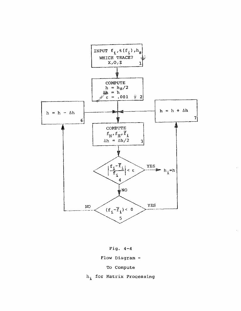
t o t h e process ing blocks i n t h e flow diagram of Fig. 4 -4 ,
1. Input f i , t(fl), hsl and t r a c e des igna to r (X, 0 , o r
Z-Trace)
2 . Compute t r i a l value of hi
- 3 . Compute fN, fH , f i , Ah. The value of f H (h) is obtained
by inver se cube i n t e r p o l a t i o n v e r t i c a l l y with r e s p e c t t o t
t r u e he igh t and l i n e a r i n t e r p o l a t i o n h o r i z o n t a l l y wi th
r e s p e c t t o t ime.
NO, go t o s t e p 5 .
YES, hi = 11. RETURN t o c a l l i n g program.
I INPUT fi,t(fi) ,hsl
WHICH TRACE3
Fig, 4-4
Flow Diagram - To Compute
hi for Matrix Processing
- 5. I f ( f i - f i ) < 0
NO, go t o s t ep 6 .
YES, go t o s t e p 7.
6 . Compute next t r i a l value, h = h - Ah
7. Compute next t r i a l value, h q h + Ah
POSITIL'E SLOPE
FIGURE 4-5
The Matrix method o f reduc ing t o p s i d e s o w a e r ionograms t o 'v.
e l e c t r o n d e n s i t y p r o f i l e s r e q u i r e s an i n i t i a l e s t i m a t e o f M(h)
a s r e p r e s e n t e d by a mathematical model. I n o t h e r words, an
i n i t i a l se t of va lues f o r - a are r e q u i r e d . This i s S t e p 3 i n
t h e flow diagram of F ig . 4-30
While t h e program f o r t h e Matr ix method is under development,
i t would be w e l l t o s t a r t w i t h an i n i t i a l f u n c t i o n N(h, - a) t h a t
i s reasonably c l o s e t o an a c t u a l N (h ) p r o f i l e computed by
e i t h e r Forward o r I n v e r s e Process ing . Program NHMODEL was
developed i n o r d e r t o curve f i t a v a r i e t y of d i f f e r e n t N(h)
p r o f i l e s d u r i n g t h e i n v e s t i g a t i o n o f ways t o adequa te ly model
an N(h) p r o f i l e . Some of t h e s u b r o u t i n e s such as CALC and MXV
can b e used d i r e c t l y i n t h e o v e r a l l Matr ix program. Other
s u b r o u t i n e s such a s COST and STEP would be modif ied f o r u se
i n t h e f low diagram o f F ig . 4 - 3 .
Program NI-IPIODEL was developed us ing a t ime s h a r e computer
t - - n i l 'I'f~cl program i s w r i t t e n mostly i n POR'llRAN I V w i t h
solnc v a r i a t i o n s t l l a t were permitted and o t h e r s r equ i r ed by
Ty l~ l~ha re FOL:Z'lt?iN I V . L)iffererrcer i n tkc? v a r i a b l e names i n t h e
program and t h e nomenclature i n paragraph 4 . 1 ar ise due t o t h e
f a c t t h a t Program NHMODEL is a r e v i s i o n o f a s t a n d a r d As t roda t a
program and i t was convenient t o minimize changes i n the
v a r i a b l e name s t r u c t u r e .
A complete l i s t i n g o f Program NHMODEL is inc luded s t a r t i n g on
page IV-34, The numbers i n t h e l e f t hand column o f each page
a r e l i n e numbers t h a t are used i n the t i m e s h a r e mode o f
o p e r a t i o n , They are convenien t f o r r e f e r e n c e b u t are n o t p a r t
o f t h e a c t u a l program.
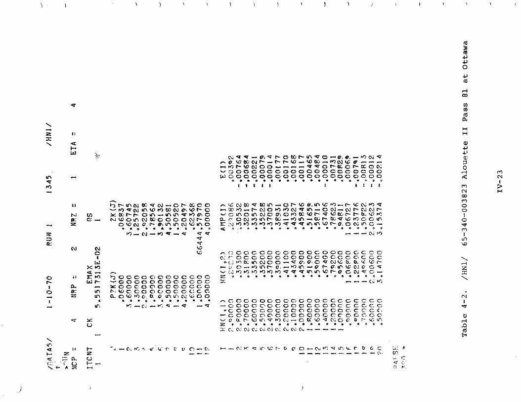
A flow diagram o f program NHMODEL i s inc luded s t a r t i n g on
page IV-33a. The r e s u l t s ob t a ined from curve f i t t i n g t h e N(h)
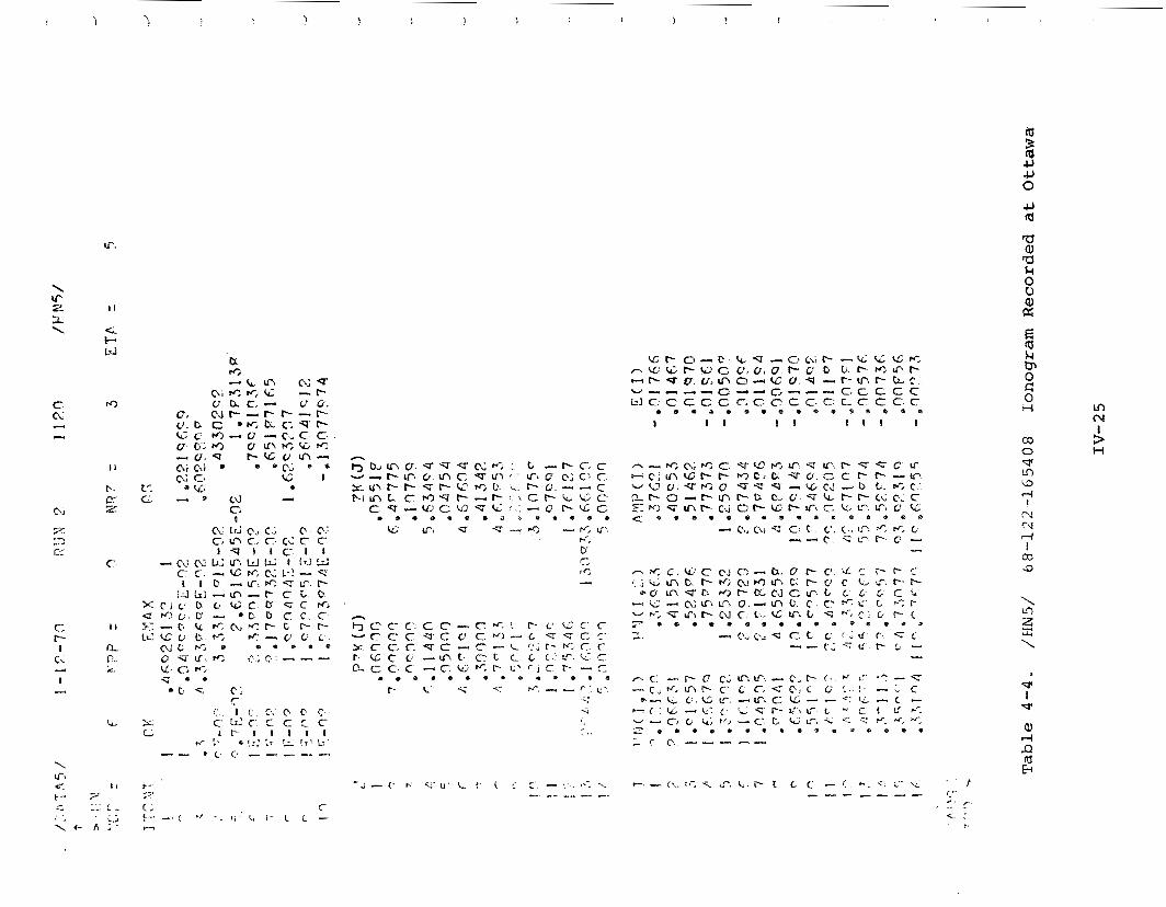
p r o f i l e s from f o u r d i f f e r e n t ionograms are sl~own i n Tables 4 - 1
through 4-5.
I n p u t d a t a i s s e t up i n t h e DATA s t a t e m e n t s , l i n e s 138 through 1 4 4 .
NCP = numbear o f complex p o l e s
NRP = number of r e a l p o l e s
NRZ = number of z e r o s a t t h e o r i g i n
The l a s t two elements of a r r a y ZK are t h e s c a l e f a c t o r p , and t h e
change of v a r i a b l e c o n s t a n t q . S c a l e f a c t o r p is modif ied on
each i t e r a t i o n a t l i n e s 580 and 8 2 4 , b u t q remains c o n s t a n t
throughout t h e program. I n l i n e 162, K is d e f i n e d a s t h e number
of degrees o f freedom i n t h e N(hi, - a) model.
A~-r,-iy IfN i s a two-dimensional a r r a y which c o n t a i n s t h e i n p u t
~ , r c . s c ~ - i p t i o n vec to r , which i s t h e N(hi) p r o f i l e t o be cu rve f i t .
The (WN ( I , 1) , I = 1 ,KL) are v a l u e s of t r u e h e i g h t i n u n i t s o f
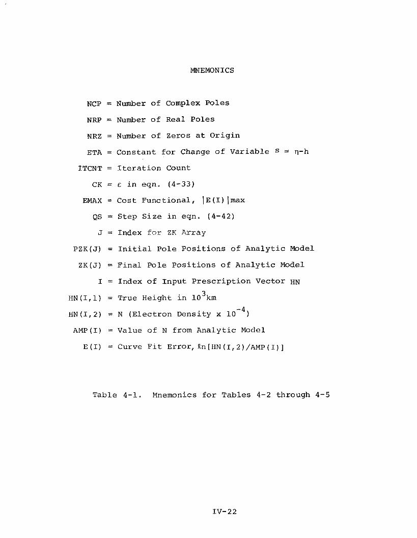
MNEMONICS
NCP = Number o f Complex P o l e s
NRP = Number o f R e a l P o l e s
NRZ = Number o f Zeros a t O r i g i n
ETA = C o n s t a n t f o r Change of V a r i a b l e s = q-h
ITCNT = I t e r a t i o n CaWnt
CK = E i n eqn . (4-33)
EMAX = C o s t F u n c t i o n a l , I E ( 1 ) (max
QS = S t e p S i z e i n eqn . (4-42)
J = Index f o r Z K Ar ray
PZK(J) = I n i t i a l P o l e P o s i t i o n s o f A n a l y t i c Model
Z K ( J ) = F i n a l P o l e P o s i t i o n s o f A n a l y t i c Model
I = Index o f I n p u t P r e s c r i p t i o n V e c t o r HN
H N ( 1 , l ) = True H e i g h t i n 10'km
HN(I.2) = N ( E l e c t r o n D e n s i t y x
AMP(1) = Value o f N from A n a l y t i c Model
E ( I ) = Curve F i t E r r o r , Rn [HN ( I , AMP ( I ) ]
T a b l e 4 - 1 , Mnemonics f o r T a b l e s 4-2 th rough 4-5
C\] C\i W G G
@ W
x m -a --. h
$ 1 E m ~ Q t 0 0 0 0 0 0 C C 0 6 W r - w G a C O O G O C O C O C ~
a X G O C O ~ C C O O C C O a- M b - W C C O O O O C G C G C . z tn a o w m ~ a o tny\c\:cr;oo
e . . . . . . . e e . e 0
In C c . C % : - N ; S - Q - V
L
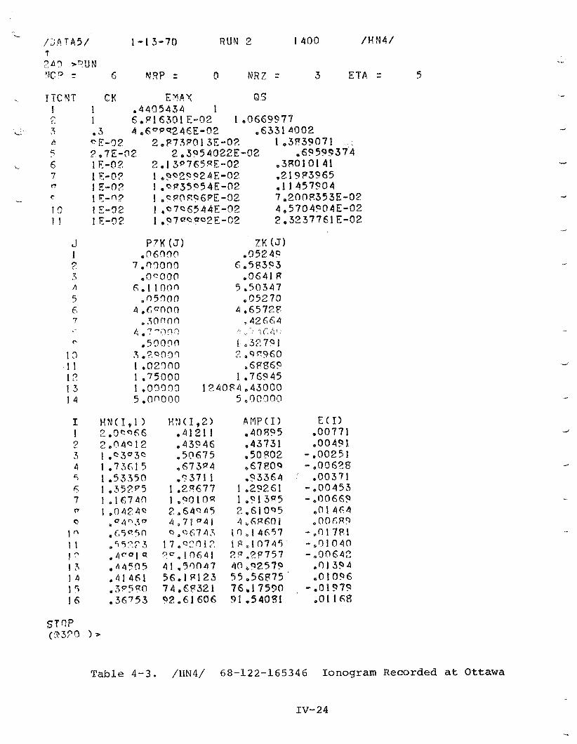
/ ,P rA5 / 1 - 1 3-70 R U N 2 1400 / K N 4 / ? T d q >n!JN 1 ~r 6 N??P = I! N R Z = 3 ETA = 5
I T C Y T CK E Y A X QC; ! n
1 .4405434 1 i. J 5.Q103C)l E-02 1 .0669977
L." 3 a 3 4 .GQps246E-02 .633141302 A "E-32 ZeP73P01 3E-02 1.3P39071 . E ?,7E-02 2,395 4022E-02 .6?5(3?3374 6 1 F-02 2 , I 39765QE-02 ,3801 01 41 7 1 E-02 I ,?@2QP24E-02 ,219P3965 n 1 E-02 1 ,QP35?54E-02 .11457904
..- r 1 F-q? 1 ,QpDRP6?E-02 7,2008353E-02 1 !! 1 E-02 1 ,Q7Q6544E-02 4,5704P04E-02 9 J 1 E-02 1 .Q7s@QQ2E-02 2 , 3 2 3 7 7 6 1 E-02
Table 4-3, /HN4/ 68-122-165346 Ionogram Recorded at O t t a w a
IX to - L l n C G Q
0 1 rs, rr, W - r u a c , + C Q .
0, C J P - P F - l - V ; C c . ~ j a . c ; - r - (L: c . a - u - C , C c.. uci,rr) UIf\FC,Grr; - u , - r ~ u r n -
C.J * * 0 c< 0 5
0 3 C G I t', a u. .
- 0 CQ C. I
cLLLc2c; @ . C < C; L l C.. CI. c; C C- t P l l C l l
-c,) \pi w r * t d !i t [ ? . J f 5 1 c' C , - '.c tC b! - F
I I 0 --. u-: rr; -7. - LP. I- l.3 (r~ - tn --. r c L. CI
)<:t]c: O C. U C fF G C fl, ct? V?,?,L' --. .e o. C: c. C 5;-c. u, c c ~ r s : r - c# r-t- LicL; O w, e-c! L ' C .
O J C ' C , 0 0 0 e m * 0 G u , r ; , : , ;c:--- CL. C, rr; < n o
0 6 . c.; (r
c: , I c , C\' @ c. c. x. C'. Ci c. c c CC C C. I t - I I I I I
b*, !. 0 L; i r !& [ , I TZ' -- . C . C . ---- d
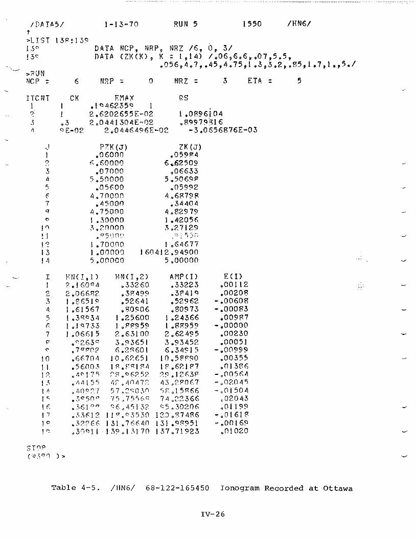
/ P A T A S / 1-13-70 R U N 5 1550 /HN6/ r >LIST 13F: 13Q 13" DATA NCP, NRP, NRZ / 6 s O 9 3 / 1 3c DATA (ZK(KI9 K = 1,141 / 8 0 6 9 6 , 6 , , 0 7 9 5 . 5 ,
a05694e79e4594e7591 e993*290g591 e 7 8 1 o p 5 * /
>RUN (YCP = 6 N3P = 0 NRZ = 3 ETA = 5
I T C N T CK EZBX 6 S 1 1 , lQ46235Q I ? I 2,6202655E-02 1,0896i04 3 * 3 2,0441 304E-02 . 8 ~ 9 7 9 ' ~ 1 6 /I Q Z-02 2,04464P6E-02 -3,0656876E-03
P7# (J) 71< (J) ,060On .05PF'4
6,60009 6 e62509 .07000 .06633
51,5'1000 5,506PP .05600 ,05C?2
4.71)OOO 4,6879R .45000 .34 40 4
4.95000 4,82979 1 ,30000 1 ,42056 , ~ , ~ n n o r , 3,27129 , "5')q') 2 4 'J:?
1 ,70000 1,646377 1 , 0 0 0 0 ~ 160412,94900 5 ,00000 5,00000
Table 4 - 5 . /IIN6/ 6 8 - 1 2 2 - 1 6 5 4 5 0 I o n o g r a m R e c o r d e d a t O t t a w a
l o 3 km. The HN ( I , 2 ) a r e t h e r e l a t e d v a l u e s of e l e c t r o n
4 d e n s i t y d i v i d e d by 10 . KL is t h e number o f e lements i n t h e
p r e s c r i p t i o n v e c t o r .
The program is i n i t i a l i z e d i n l i n e s 148 through 172. A t l i n e s 174
and 1 7 6 , t h e Z K a r r a y i s s t o r e d i n P Z K f o r comparison on f i n a l
p r i n t o u t .
nt l i n e s 178 and 180, t h e change o f v a r i a b l e computation t a k e s
p l a c e ,
s - = n - n i i irdm eqn. (4-2)
i = 1, 2! . . e m f I
Subrout ine CALC, which i s f i r s t c a l l e d a t l i n e 188, computes
N ( s i ) , eqn. (4 -2 ) , a s AMP(I), u s i n g t h e va lues of - u i n a r r a y ZK.
I n l i n e 580, t h e s c a l e f a c t o r p is computed i n i t i a l l y so t h a t
i n l i n e 584
This f o r c e s t h e two curves N(h) and N(hi, - n) t o c r o s s a t t h e
t e n t h l amina t ion boundary,
I n Subrout ine COST, which i s f i r s t c a l l e d a t l i n e 196, t h e
d i sc repancy v e c t o r E ( 1 ) i s computed i n l i n e 816. This is s imilar
t o vector E - i n cqn, ( 4 - 1 0 ) . I n the same DO loop t h e sum set of
E ( I ) is accumulated s o t h a t t h e mean va lue can b e computed i n
l i n e 820. The mean va lue of E(1) i s removed i n l i n e 830 which
i s e q u i v a l e n t t o changing t h e scale f a c t o r P by a t e r m c a l l e d
EXM i n l i n e 822. The s c a l e f a c t o r c o r r e c t i o n t a k e s p l a c e i n
l i n e 824. On t h e l a s t i t e r a t i o n , t h e s c a l e f a c t o r c o r r e c t i o n
is a p p l i e d t o AMP(1) i n l i n e 314 f o r p r i n t o u t . I n t h e DO loop
l i n e s 828 through 836, t h e maximum a b s o l u t e va lue o f E ( 1 ) i s de f ined
as EMAX.
I n Program NHMODEL, EMAX i s used as the c o s t f u n c t i o n a l and t h e
program i s structured t o rrti n j rn izo RMRXI a l though it minimizes a l l
o t h e r va lues of E ( 1 ) a s w e l l . Beginning a t l i n e 838, i f EMAX > .5
a d i f f e r e n t s c a l e f a c t o r is computed a s ER. Th is i s used t o
s c a l e down t h e d i sc repancy v e c t o r E ( 1 ) i n l i n e 844 s o t h a t t h e
maximum va lue o f - E i n t h e m a t r i x equa t ion does no t exceed 0.5.
This p reven t s a d i v e r g e n t c o n d i t i o n from developing i f t h e
i n i t i a l v a l u e s o f ZK are n o t very good.
S ta tement 100 a t l i n e 198 i s t h e r e e n t r y p o i n t f o r t h e m a j o r -
i t e r a t i v e loop and i s c a l l e d a t l i n e 298, There are t h r e e e x i t
c o n d i t i o n s from t h i s major loop a t l i n e s 202, 208, and 209. I
'L'l~cl s l c m c ~ ~ t s of t l l c . m a t r i x of' p a r t i a l derivatives f l ( f IL) arc
computeci i n Subrout ine GEND, which i s c a l l e d a t l i n e 216.
These a r e s i m i l a r t o t h e e lements aik of eqn. (4 -9) , b u t t h e
D(1,L) can be computed d i r e c t l y because N(h, - a ) is an a n a l y t i c
f u n c t i o n o f - a and is t h e model o f the curve t o b e f i t t e d . The
e lements are computed as t h e p a r t i a l d e r i v a t i v e o f t h e n a t u r a l
logar i thm o f t h e f u n c t i o n N ( s , - a ) w i t h r e s p e c t t o - ce a s g iven by
where t h e n o t a t i o n D(1,L) i s s i m i l a r t o aik i n eqn. (4-9) .
So f a r i n t h e program we have developed a m a t r i x equa t ion
where DK is t h e program name f o r t h e adjustment v e c t o r A q . The
s i m i l a r i t y w i t h eqn. (4-10) i s obvious . Both s i d e s of eqn.
(4-29) a r e m u l t i p l i e d by - D~ i n l i n e s 224 through 2 4 0 . I n t h e program
and
S ince A - i s a symmetric ma t r ix , on ly t h e terms on and above t h e
main d i agona l a r e computed d i r e c t l y . Terms below t h e main
d i agona l a r e f i l l e d i n a t l i n e 254.
Under some c o n d i t i o n s m a t r i x A - can be poor ly condi t ioned s o t h a t it
cannot bc propcrly i n v e r t e d . T h i s c o n d i t i o n is prevented by adding
a c o ~ l s t ~ ~ n t z Cl< t o cach t - c r m of t h c main d i agona l a t l i n e 250. Th i s
a l t e r s t h e ma t r ix equa t ion which i s then compensated by adding
t h e p rope r c o r r e c t i o n t e r m t o t h e o t h e r s i d e of t h e equa t ion .
Assume a m a t r i x equa t ion o f t h e form
~t fo l lows t h a t
where I = i d e n t i t y ma t r ix
I n t h e program
l i n e 266
S ince DK is t h e unknown i n t h e m a t r i x equa t ion , t h e f i r s t t r i a l
va lue o f DK f o r eqn. ( 4 - 3 3 ) i s t h e prev ious va lue from t h e p r i o r
i t e r a t i o n . DK is then computed i n Subrout ine MXV which g i v e s a
b e t t e r va lue of - Dl< fo r eyn, ( 4 - 3 3 ) . This is repeated f o u r t i m e s
i n l i n e s 2 6 2 tllrc>ucjh 2 7 4 , cncll t i m e improving the va lue of DK.
Under c e r t a i n c o n d i t i o n s CK i s r e v i s e d downward, l i n e s 276 through
280, s o th 'a t
.01 < CK 1, - ( 4 - 3 4 )
This reduces t h e produc t t e r m EX - i n eqn. ( 4 - 3 3 ) s o t h a t it becomes
less and less s i g n i l i c a l i t i n t h e va lue of B1. A-
Subrout ine MXV 1241 computes - X i n eqn. (4-32) w i t h o u t e v a l u a t i n g
-1 A . F o r a 10 x 10 m a t r i x t h i s r e q u i r e s on ly about one h a l f t h e - computer CPU c y c l e s compared w i t h e v a l u a t i n g X - us ing t h e
equa t ion
MXV i s modif ied from a g e n e r a l i z e d ma t r ix i n v e r s i o n s u b r o u t i n e
from McCracksn. ["I
The magnitude of adjustment v e c t o r - DK can be opt imized t o g i v e
maximum r e d u c t i o n i n the c o s t f u n c t i o n a l EMAX. This i s accomplished
i n Subrout ine STEP us ing a Golden S e c t i o n Search ["I * I n t h e
program, t h e s t e p s i z e QS becomes a s c a l a r m u l t i p l i e r on - DK i n
l i n e s 928, 952, 966, and 994.
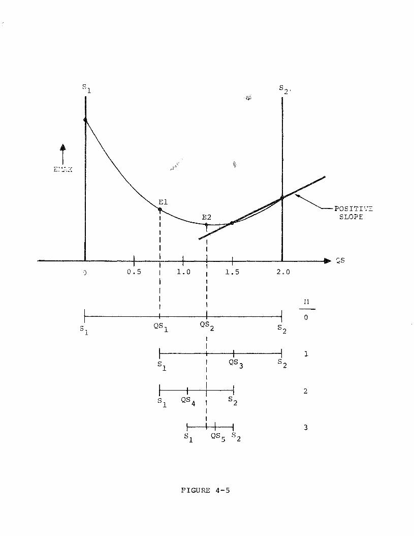
The boundar ies of t h e s ea rch i n t e r v a l a r e S1 and S2, w i t h i n i t i a l
va lues o f 0 and 1 r e s p e c t i v e l y i n l i n e s 918 and 920. I n t h e
f i r s t p a r t of STEP, t h r u l i n e 944, S2 is inc reased by increments
oE 0.5, l i n e 936, u n t i l a l i n e t h r u two consecu t ive va lues of
EMAX has a p o s i t i v e s l o p e , l i n e 934, This e s t a b l i s h e s t h e minimum
v a l u e of E P W as l y i n g somewhere between S1 and S2, a s shown i n
Fig . 4 -5 .
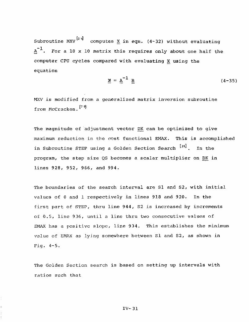
The Golden S e c t i o n s e a r c h i s based on s e t t i n g up i n t e r v a l s w i t h
r a t i o s such t h a t
The search for minimum E M starts at line 948 with M = 0.
Compute the following:
El = EMAX
lines 948-958 lQS1 = .382 (52 - 51)
E2 = EMAX
lines 962-972 IOSZ = .618(52 - 51)
Then compare to see which of El and E2 is larger, line 978.
If E2 < El
then QS1 < QS < S2
We reduce the search interval by making
On t h e n e x t i t e r a t i o n with M = 1, El = E2 and a new E2 is computed.
E2 = EMAX (4 -41)
Lines 962-972 /QSJ = Sl + .618(S2 - S1)
By us ing t h e r a t i o s i n t h e Golden S e c t i o n s e a r c h , it i s on ly
necessary t o compute one new v a l u e of EMAX p e r i t e r a t i o n . A f t e r
t e n i t e r a t i o n s , t h e s t e p s i z e QS f o r minimum EMAX has been
determined. The loop e x i t s a t l i n e 976 w i t h M > 9. The s c a l a r
mu1 t i p l i c a t i o n
occurs a t l i n e 994, fol lowed by a r e t u r n t o t h e main program.
A l l t h e s t a t e v a r i a b l e s should remain p o s i t i v e . I f any e lements
become n e g a t i v e , they a r e fo rced p o s i t i v e a t l i n e 294. This
completes t h e major i t e r a t i v e loop of Program NHMODEL. A d e t a i l e d
f l o w diagram f o r t h e Program NIIMODEL i s shown on F igu res 4-6
through 4-11 , and a program l i s t i s provided i n Table 4-6.
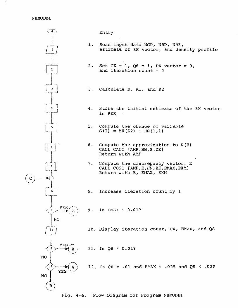
NHMODEL
Entry
1, Read i n p u t d a t a NCP, NRP, NRZ, e s t i m a t e o f ZK v e c t o r , and d e n s i t y p r o f i l e
2 . S e t CK = I, QS = 1, DK vector = 0 , and i t e r a t i o n count = 0
3 . C a l c u l a t e K , K 1 , arid K 2
4 . S t o r e t h e i n i t i a l e s t i m a t e of t h e ZX v e c t o r i n P Z K
5. Compute t h e chanse of v a r i a b l e S ( I ) = Z K ( K 2 ) - I I Z J ( 1 , l )
6 . Compute t h e approximation t o N ( H ) CALL CALC [AMP,HN,S,ZK] Return wi th AMP
7 . Compute t h e d i sc repancy v e c t o r , E CALL COST [AMP,E,HN,ZK,ENX,EXM] Return w i t h E , EMAX, EXM
8. I n c r e a s e i t e r a t i o n count by 1
1 0 . Display i t e r a t i o n count , CR, EMfiX, and QS
1 2 . Is CK = .01 and EMAX < .025 and QS < .03?
NO
Fig& 4-6. Flow Diagram for Program NIIMQDEL
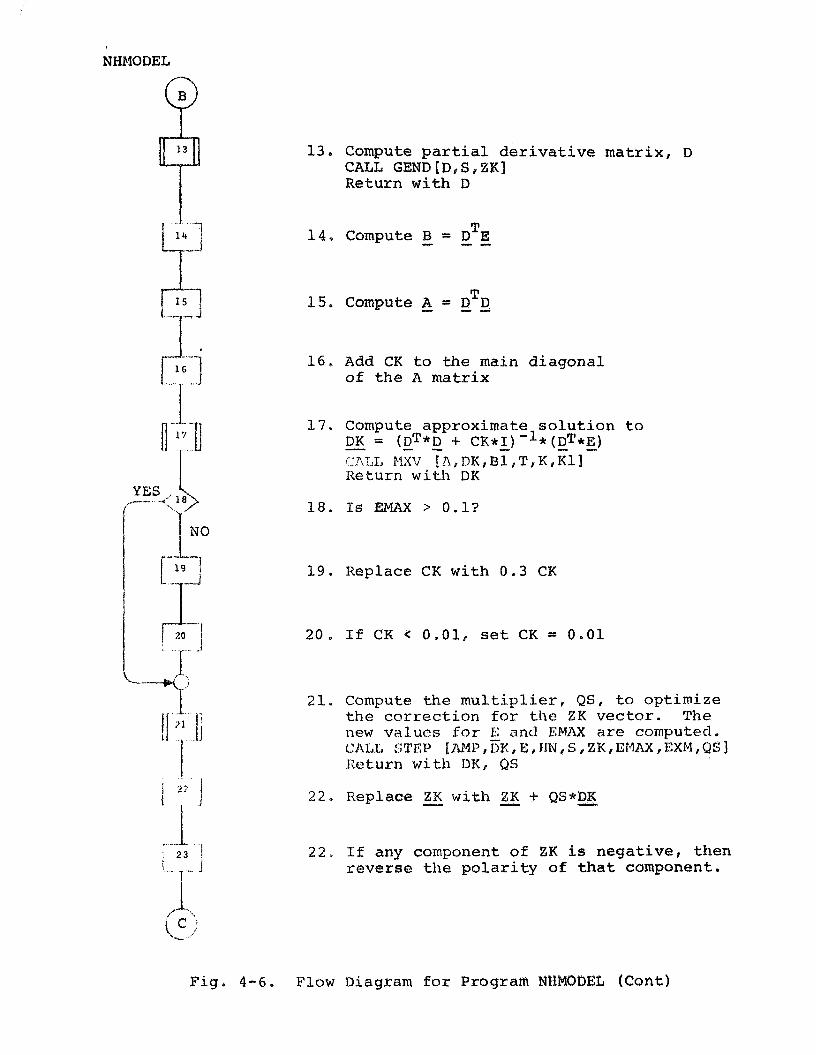
13, Compute p a r t i a l d e r i v a t i v e matr ix , D CALL GEND[D,S,ZK] Return wi th D
T 1 4 , Compute - B = D E - -
T 15. Compute A - = - D - D.
16. Add CK t o t h e main diagonal of t h e A matr ix
17 . Compute approximate s o l u t i o n t o DK = (DT*D + C K I I ) - ~ * (DT*E) - - - - - - (XLL MXV fA,DK,Bl,T,K,Kl] Return with DK
1 9 . Replace CK with 0.3 CK
2 0 , I f CK .: 0.01, s e t CK = 0.01
2 1 . Compute t h e m u l t i p l i e r , QS, t o optimize t h e co r rec t ion f o r t h e Z K vec tor . The new v + ~ l u c s fo r k; and EMAX a r e computed, CALL STEP [AMP, EK, E , JIN ,S,ZK, E14AXI EXM, QS ] Return with DK, QS
22. Replace - ZK with ZK + QS*DK - -
2 2 * I f any component of ZK i s negat ive , then reverse t h e p o l a r i t y of t h a t component.
Figl 4 - 6 , Flow Diagram f o r Program NNMODEL (Cont)
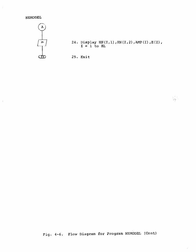
NHMODEL
24. Display HN(1,l) ,HN(I,2) ,AMP(I) , E ( I ) t f = 1 to KL
25. E x i t
Fig. 4-6. F l o w Diagram for Program NHMODEL (Cont)
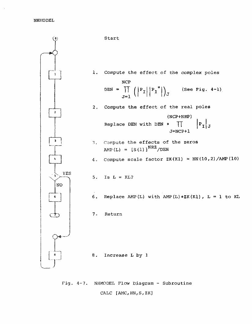
S t a r t
1. C o m p u t e t h e effect of t h e complex poles
NCP
DEN = rr ( S e e F ig . 4-1) J=1
2. C o m p u t e t h e e f fec t of t h e rea l poles
(PJCP+NRP)
R e p l a c e DEN w i t h DEN * J = N C P + l
3 . Carnpute t h e effects of the zeros
AP.TP(L) = ISU) I ~ ~ ' / D E N
4 . C o m p u t e scale fac tor Z K 4 K 1 ) = HN ( 1 0 r 2) / A m ( 1 0 )
6 . R e p l a c e AMP (L) w i t h AMP (L) *ZK ( K l ) , L = 1 t o KL
7 . R e t u r n
8 . Increase L by 1
F i g . 4-7 . NNMODEI, F l o w D i a g r a m - S u b r o u t i n e
CALC [AMC,HN,S,ZK]
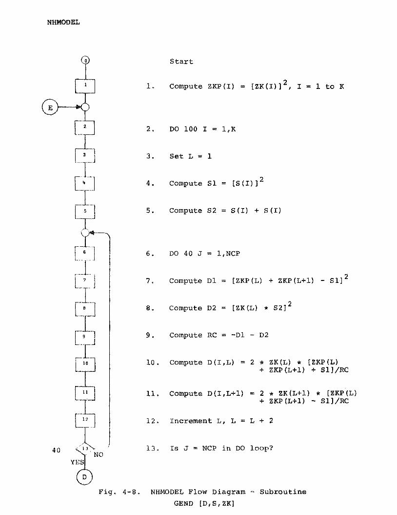
NHMODEL
Start
2 1, Compute ZKP(1) = [ Z K ( I ) ] , I = 1 to K
2 . DO 1 0 0 1 = 1 , K
3 . S e t L = l
4, Compute $ 1 - [ S ( I ) l 2
5. Compute S 2 = S (I) + S ( I )
6 . D O 4 0 J = l , N C P
7. Compute D l = [ZKP(L) + ZKP(L+l) - S l ] 2
8. Compute D2 = [ZK(L) * 521 2
9, Compute RC = - D l - D2
1 0 Compute D ( I , L ) = 2 * ZKfL) * [ZKP(L) + ZKP(LS1) + Sl] /RC
11. Compute D ( I , L + l ) = 2 * Z K ( L + ~ ) * [ZKP(L) + ZKP (LS1) - S l J / R C
12, Increment L , L = L + 2
4 0 1.3, 1s 3 = NCP i n DO 1-oap?
Fig* 4-8. NHMODEL Flow Diagram - Subroutine GEND [D, S , ZK]
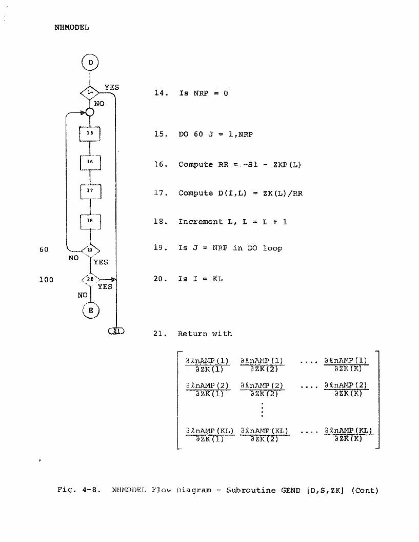
NHMODEL
DO 60 J = 1,MRP
Co~pute RR = -S1 - ZKP(L)
Compute D (I ,L) = ZK (L) /RR
Inc rement L, L = L + 1
Is J = NRP i n DO loop
Is I = KL
R e t u r n with
a R n n m ( 2 ) a R n m p ( 2 ) .... a g n ~ ~ P ( 2 ) a Z K ( 1 ) aZK(2) a Z K ( K )
Fig. 4-8. NIIbtODEL F low Diagram - S u b r o u t i n e GEND [ D , S , ZK] (Cont)
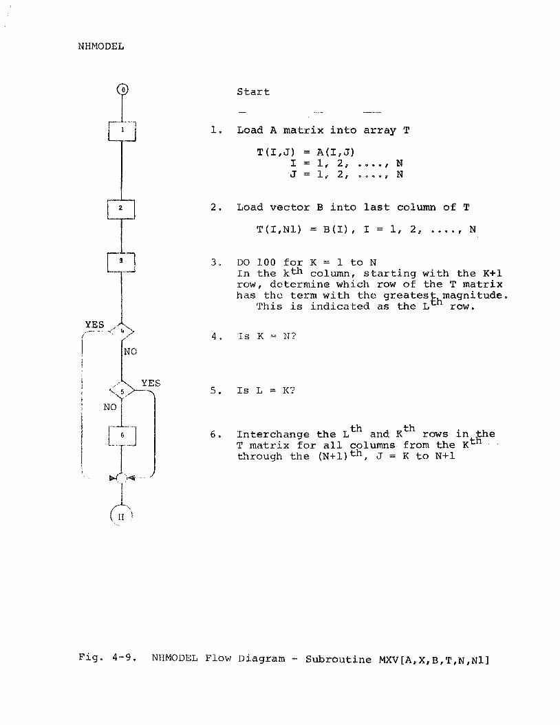
S t a r t
1. Load A matrix i n t o a r r a y T
2, Load v e c t o r B i n t o l a s t column o f T
3 , DO 100 f o r K = 1 t o N I n t h e k t h column, s t a r t i n g w i t h t h e K+1 row, de t e rmine which row o f t h e T m a t r i x ha s t h o t e r m w i t h t h e g r e a t e s t magnitude.
Th i s i s i n d i c a t e d a s t h e L~~ row.
6. I n t e r c h a n g e t h e Iith and K* rows i n t h e T m a t r i x f o r a l l columns from t h e K~~ through t h e ( N - I - ~ ) ~ ~ , J = K t o N+1
Fig . 4 - 9 . NHMODEL Flow Diagram - Subrou t ine MXV[A,X,B,T,N,Nl]
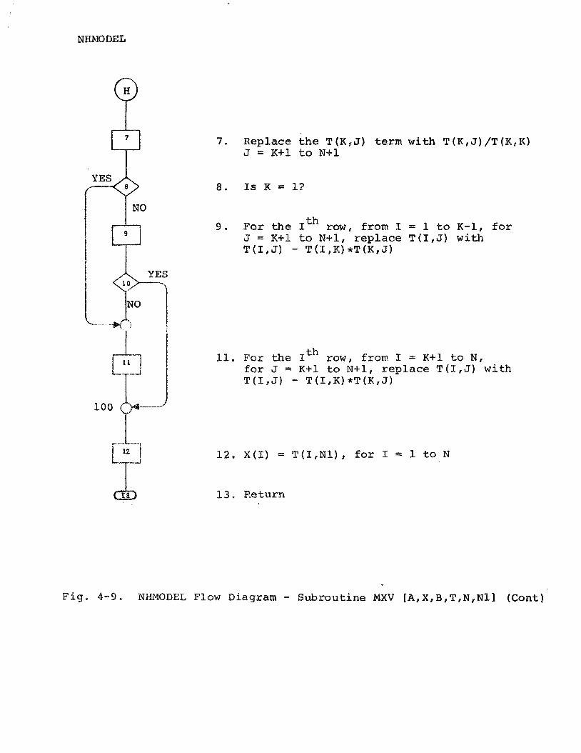
7. R e p l a c e t h e T ( K , J ) t e r m w i t h T ( K , J ) / T ( K , K ) J - K + 1 t o N + 1
9. For the Ith row, from I = 1 t o K - 1 , f o r J = K 9 1 t o M4-1, replace T ( 1 , J ) w i t h T ( I , J ) - T ( I , K ) * T ( K , J )
11. For the ith r o w , from I = K + 1 t o N, fo r J = K + 1 t o N+1, replace T ( 1 , J ) w i t h T ( I , J ) - T ( I , K ) * T ( K , J )
12. X (I) = T ( 1 , N l ) , for I = 1 t o N
F i g . 4-9, MHMODEL Flow Diagram - Subroutine MXV [ A , X , B , T , N , N Z I ( C o n t )
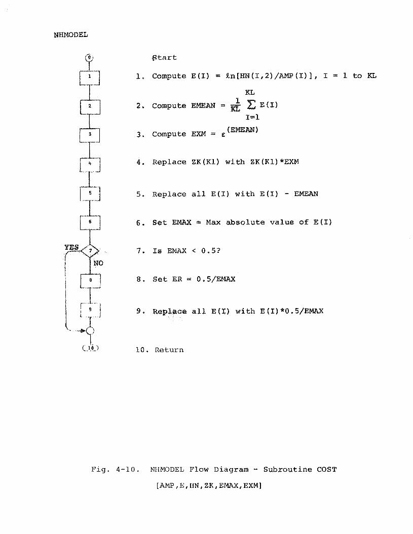
1. Compute E ( 1 ) = R ~ [ H N ( I , ~ ) / A M P (I) I , I = 1 t o KL
KL 1
2. Compute = E ( I )
1-1
3 . Compute Em = E (ErnE4EJ)
4, R e p l a c e ZK ( K I ) w i t h ZK ( K l ) *EXM
5. R e p l a c e a l l E ( 1 ) w i t h E ( I ) - EMEAN
6. Sat E = Max absolute va lue of E ( 1 )
8 . S e t ER = O . S / E W
9 R@gl&oe a l l E ( I ) w i t h E (1) * 0 . 5 / E M
I.
(2 0) 10, Return
Fig . 4 -10 . NIirJIODEL Flow D i a g r a m - S u b r o u t i n e COST
[AMP, E , I iN , ZK , EMAX, EXM]
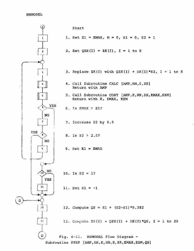
P Start
1, Set El = E B W , M = 0, Sl = 0, S2 = 1
2. Set QZK(1) = ZK(I), I = 1 to K
3. Replace ZK (I) with QZK(1) + DK(1) *S2, I = 1 to K
4. Call Subroutine CALC [AMP,HN,S,ZK] Return with AMP
5. Call Subroutine COST [AMP,E,HN,ZK,ENAX,EXM] Return with E, E W , EXM
6, Is E b f m > El?
7 , Increase S2 by 0.5
9, Set El = EMAX
11, Set Sl = -1
1 l 2 1 12, Compute QS - S1 + (S2-S1)*0.382
1 3 , Co i i t~%utc 52C (I) = QZK (I) + DK (f) *QS, I = 1 to 20
Fig. 4-11, NHMODEL Flow Diagram - Subroutine STEP [AP?IP,DK,E,HM,S,BRIE~X,EXM,9S]
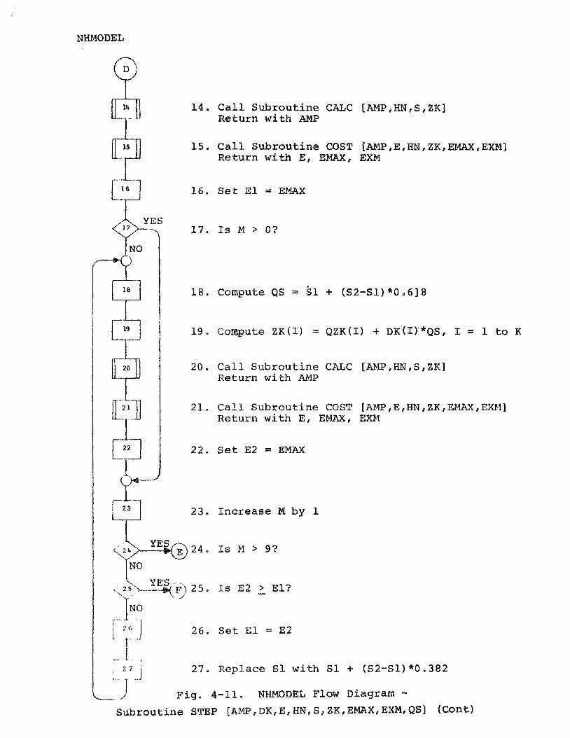
1 4 , C a l l S u b r o u t i n e CALC [AMP,HN,S,ZK] Re tu rn wi th AMP
15. C a l l S u b r o u t i n e COST [MP,E,HM,ZK,EMCEXM] Re tu rn w i t h E l E
1 6 . S e t E l - EMAX
17. Is M > O?
1 8 . Compute QS = k 1 + (52-S1) *0 ,6 ] 8
19, C o m p u t e ZK(1) = Q Z K ( 1 ) + DK(I~*QS, I = 1 t o K
2 0 . C a l l S u b r o u t i n e CALC [hMP,HN,S,ZK] Re tu rn with MlP
2 1 . C a l l s u b r o u t i n e COST [AMP,E,HN,ZK,EMAX,EXM] Re tu rn w i t h E , E M , EXM
22 . S e t E2 = EMRX
23. Increase M by 1
24. Is M > 9?
25, Is E2 > E l 3 -
2 6 , S e t El = E2
27. R e p l a c e S 1 wi th $1 + (S2-S1) *0.382
Fig. 4-11 . NHMODEL Flow ~iagram - S u b r o u t i n e STEP [AMP,DK,E, HPJ, S t ZK,EMAX,EXM,QS] ( ~ o n t )
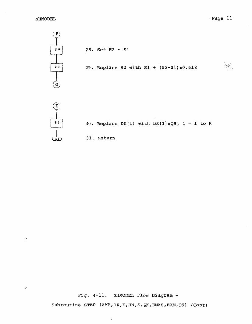
NHMODEL . Page 11
9 28. Set E2 = El
29. Replace 62 w i t h S1 + (52-S1) e0.618
4 30. Replace DK(1) with DK(I) *QS, I = 1 to K
(&J 31, R e t u r n
Fig. 4-11, NHMODEL Flow Diagram - Subroutine STEP IAMP,DK,EpHN,S, ZK,EMAS,EXM,QSJ (Cont)
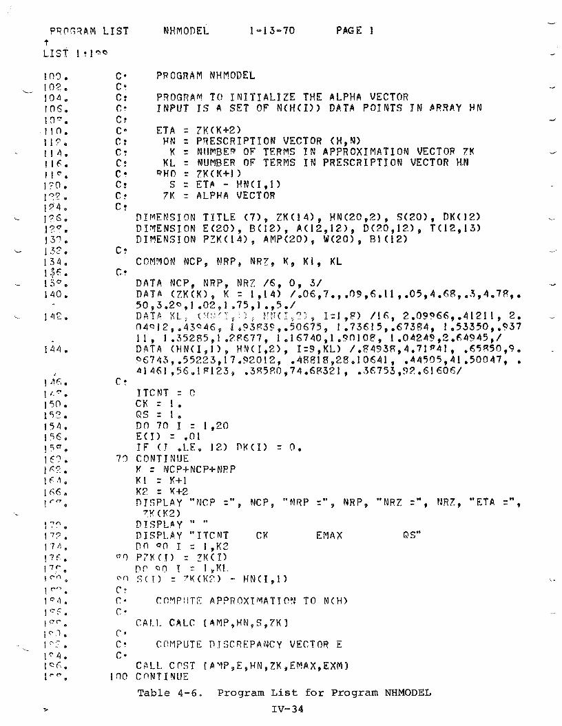
P9PG9AM LIST N H M O D E L 1 -1 3-70 PAGE 1 t LIST I
103, C P PROGRAM NHMODEL - 102, C
104 . C r P3DGRAW TO INIT f ALP ZE THE ALPHA V E C T O R 105, C? INPUT IS A SET OF N(tf(1)) DATA POINTS J N A R R A Y HN
I " " ,
C ? C e ETA = 7K(Ki-2) C r HN = PRESCRIPTION VECTOR (H,W C: K = NUNBEq OF TERMS I N APPROXIMATION VECTOR 2# C: KL. = NUMBER OF TERMS IN PRESCRIPTION VECTOR H.N C * QHO r I K ( K - 4 - 1 ) C: S = ETC - HN(191) C P 7K = ALPHA VECTOR C !,
DIMENSIQM TITLE (71, ZK(141, HN(2092), S(201, D K ( 12) DIVENSION E(201, B(12), A(lZ912) , D(20,12), T(12,13) DIMENSION PZK(141, AMP(201, W(20) , 81 (12)
C I, C0MYON NCP, MRP, N R Z , K, K1, KL
C e
D A T A NCP, NRP, NRZ /6, 0 , 3/ D A T A ( Z K ( K ) 9 K = 1,141 /e0697.,.f1996011 ,.05,4e6R9e3,407F:9. 50,3,20,1 e02,1 .75,1 ,,5,/ D A T F . X L , I. i!l lIb0>, 1-1 ,P) / I 6 , 2,09?66,.41211, 2 , 0 4 Q 12, , 43Q46 , 4 , ? 3 ~ 3 9 , ,50675, 1.7361 5 , .67384, 1 ,53350, ,037 1 1 9 1a352F(591 e2V677, 1e1674091.r?RIOf?9 lo0424!9,?,e64945,/ D A T A 0 4 N ( I , l ) , HN(192), 1=3,KL) / , t?493R,4 .71~4l9 . 6 5 9 5 0 , 9 . a67439 ,55223*1 7e920129 c4&418928.1 0641 , .44S05,4lb5O047, e
4 1 461 956e1V123, .385R0,74,683219 e36753,9!?061606/ C ?
f T C N T = (!
CK = 1 . QS = 1 , Dn 70 I = 1,20 E ( I > = @ O l I F ( T .L.E, 12) D K ( I ) = n,
77 CONTINME F = NCP+NCP+NF?P KI = K+1 K? = Y+2 DISPLAY "NCP =", NCP, "NRP =", NRP, " N R Z =", NRZ, "ETA =",
7 Y (K2) DISPLAY " "
DISPL,AY "ITCNT CK EMAX C;I S" P O QD T = I ,K2
Q q P7KlT) = ? # ( I ) p f a 0 1 = 1 ,KL
Dfl S ( T ) r 'K(K3) - HM(I,l) t * (1 Cf?YP?ITL? A P P R O X T M A T Z D N T O N ( H ) (1
CAI- I , C A L C t AMP9HN,S,7K3 r * C ? COMPUTE P T S C S E P A N C Y V E C T O R E C a
CbLL. CPST IPYP,E,HN,ZK,EMAX,EXMI I n0 C nNT I NUE
Table 4-6. Program List f o r Program NHMODEL
IV-34
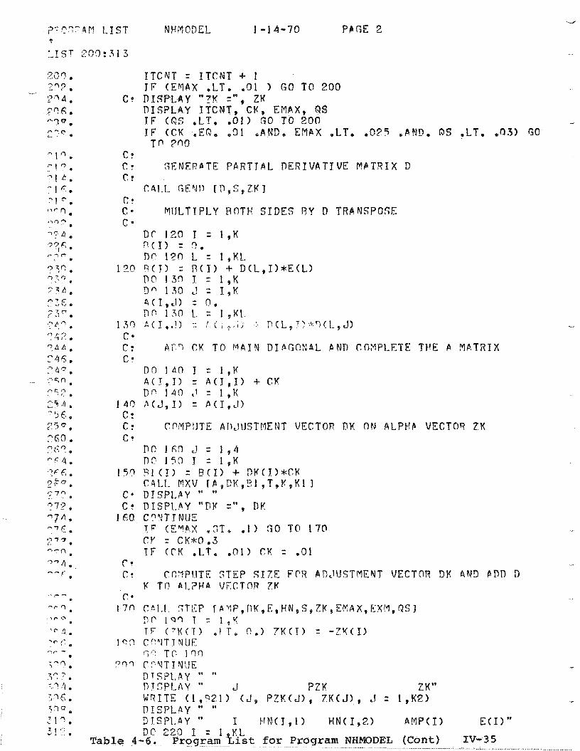
1 - 1 4-70 PCGE 2
I T C Y T = I T C N T + 1 J F ( E V A X .LT, .01 G O TO 200
C* D I S P L A Y " P K =", ZK DISPLAY I T C N T , C K , EMAX, QS TF (65 .LT. .01) G O TO 200 -,
I F (CK .E6, .91 . A N D , EMbX .LT, . O P 5 .AMD. OS .LT. . 03) GC! T P ?no
C F
C 7 G E N E S P T E P P R T J A L D E R I V A T I V E M B T R I X P C:
C4l . l . GEbJl ' , (17, S $, ZV 3 C t C * YIjIaTIPI,Y BOTH SIDES R Y n TRANSPOSE C *
D f 120 I = 1 , K ? ( I ) = 3 , n r 12r1 L = ~ , K L
1?0 R(T) = D ( 1 ) + D ( L , I ) * E ( L ) DC\ 13n I = I , K D n 1 3 0 C = J 9 K 4 ( T , e J ) = 0, nr? 130 L = I , K L .
13n A c i c l , c ! > x ,' t d I ; : 7 t \ - 9 ? > k 9 ( 1 - 9 t ! ) C * C : CK T O M 4 I N D I A G O N A L h N D COMPLETE THE A 9 A T R I X C e
D o I40 I = I , % A ( J , J > = A ( S 9 1 ) + CK D I I 1 4 0 , I = I * K
4 I = P ( I p J ) c l C: rPMP1ITE All,I1JSTMENT VECTOR DK O N ALPt?C VECTOR Z K C *
P O 1 G f l J = 1 8 4 DP 150 I = 1 , K
15n W I ) = B ( I ) + nvcI)*cK r 4 L L P X V l f i , D K , ! 3 1 , T p Y , K 1 I
C a DISPL,hY " '"
C ? DESPLbY "DK =", DK 1 66 C?VT X NIIE
T c ( E W A X .ST, , l ) G O TO 170 CY = c K ~ 0 . 3 IF (CN . L T , .01) CK = . 0 1
r e - C ? CO?lPIITE STEP SIZE FCX AD,IUSTMEhlT VECTOR DK AF3D PDD D
F TO A t , ? V A VECTDP 7tf r *
1713 Cfil.1 5TKP f PYP,llK,E,HN,S, ZK ,EMAX9FJXIYf9C?Sl l?f' 1Qf-l 7 z 1 * q TF 1 . I T , 9,) 7K(T) = - 7 Y ( I )
I Qfl CT'nJT 1 N1JE I ; ( . ' TP 1'30
V ' J ~ c ? f JT I V!JE - DTSPL,AY " " TJTSPLAY " ,-I PZK ZK" WPITE ( l , Q 2 1 ) (J, P Z K ( J ) , Z K ( J ) , = 1,K2) - n I s P t n y 9TSPI-AY " I VN(I , I> H N ( I 1 2 ) APrrP(f E ( 1 ) " D P 2 2 0 I = 1 K.L
Table 4-6. Program h s t for Program NHMODEL (Cont ) XV-35 - - -
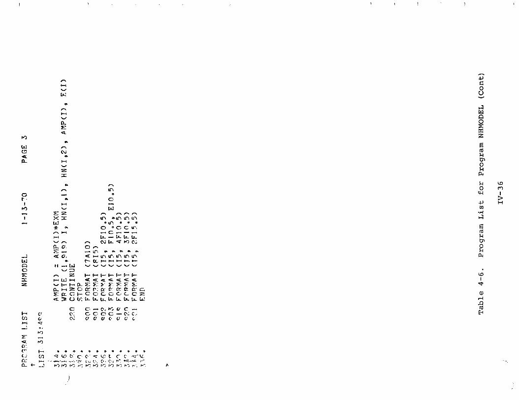
m n n tn - Q m C.
H -.I
V W .E Z n nnn X I tn " n m m W .LP. c Q 6
-)C 0 Q C C r r * n W - c 4 - - M L-rLLLtF w n n N L r - P ' I C u n u. o fi E - dip, e m m a * c i ~ V , Q ulntr~mLnm
R ( 4 ~ U M U h k ) I @ W w u v v w v w
- 3 n ;;E + + l - + t " + f - H W W Q Q Q Q a L I = C U F + ~ . E Z F . ' E - Z Z S ~ : n . . W Z C r r P : ~ f - - ~ C ~ C E & C t - C C c C C ~ C z Q3UV.bkkttbLL.d
C C - e . , W , U C - 0: C C C C - C ' ; c > (N C ' C V L . C / ' C C
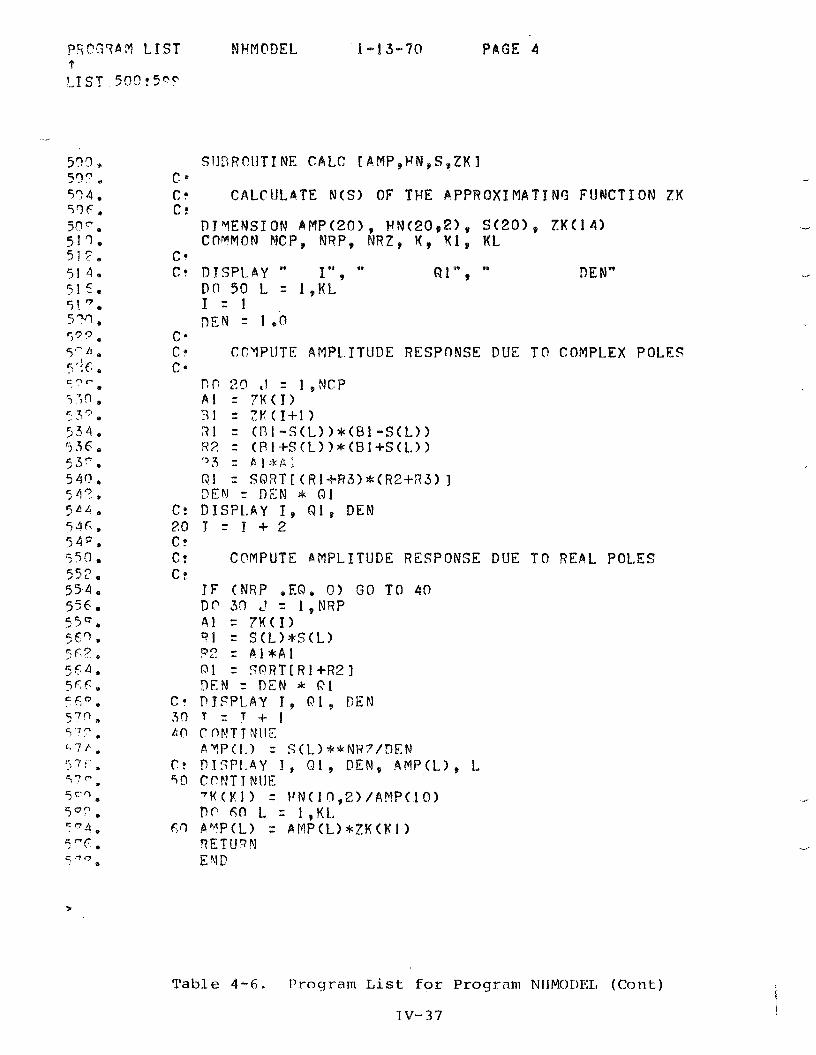
P4?15?APl LIST NWMODEL t 1.-I ST 50Q r 5e9
1-13-70 PAGE 4
SlJ3Rf?lJTf NE CALC [AMP,HN,S,ZKI C e C P CALCUL4TE N ( S ) OF THE APPROXIMATING FlJPJCTION ZK C:
D J Y E N S I O N w 1 ~ ( 2 0 ) , ~ ~ ( 2 0 ~ 2 ) , ~ ( 2 ~ 1 , Z K ( ~ 4 ) COMMON MCP, NQP, NRZ, Y, XI, K t
C * C ? ~ ~ S P I , B Y I " , 611 Fv P I ) E A ) ~
Dn 50 L = 1 ,KL I = 1 DEN = 1 .O
C - C * CCYPLJTE AMPL. ITUDE RESPONSE DUE T O COMPLEX POLES C e
D O 20 , I = 1,NCP A 1 = 7 K ( J ) 31 = 7 K ( I + l ) ; ? I = ( t 3 l - S ( L ) ) * ( B I - S ( L ) ) 82 = ( R I + S ( L > ) * ( B l + S ( L > ) ' 3 3 = F 1 $ R : Q I = SORTI(Hl+F?3>*(R2+R3) I 3Eh! = DEN * ( 3 1
C! DISPL.AY I , Q 1 , D E N 3.0 I = J + 2 C? C: COMPUTE AMPLITUDE RESPONSE D U E TO REFL POLES C:
I F ( N R P .EO, 0 ) G O T O 40 D p 30 L! = 1,NRP A 1 = 7 K ( I ) Q l = S ( L ) * S ( L ) ?2 = C l * A I 01 = FORT[Rl+R21 D E N = DEN * R 1
C a DJFPLAY I , R 1 , DEN , T r , T Z T + I 110 C OF!T T VllE
= S(L,)**NH7/T)EN fr DISPl .bY T , Q 1 , D E N , AMP(L), L 5 0 CPNTT NlJE
7K(FI) = HW(ln92)/WMP(1O) D P 60 L = 1 , K L .
6Q PwP(L) = BPP(L)*ZK(KI) '7EfIJqN E Y D
Tab le 4 - 6 . Program L i s t f o r Progrnni NIIMC)I)E:I, ( C o t l t )
'IV-37

P F I ~ S R A X L I S T NHMODEL 1 - 1 3-70 PAGE 5 ? LTST 6OT:EQQ
S:IB?OUTINE GEND [D9S9ZKI C ? C: G E N E R A T E S D M A T R I X OF PARTIAL D E R I V P T I VES C F
DIMENSION S(20) , Z X C 1 4 1 , ZKP(12) D(20912) COMMON WCP, MRP, N R Z B K9 Kle KL
C ? 110 10 I = 19K
10 7KP(3> = 7K(I)*?K(I) n o I o n I = I , K L L = l $ 1 = S(I)*S(I> S? = S(I> + S(I)
c 2
C : TERMS FOR CGMPLEX POLES C ?
D P 4 0 .I = 1 ,NCP Dl = (TKP(L>+7KP<L+l)-Sl)**2 DZ = (?K(L)*S2)**2 F C = - 3 - i'.': I f ( . I , L ) = (P,*ZK(L) *(ZKP(L)+ZKP(L+l )+S1 )),/RC D(I,L+1) = (2,*ZK(L+l)*(ZKP(L)+ZKP(L+l)-SI))/RC
4 0 L = L + 2 C: C: TERMS FOR REAL POLES c:
I F (NRP .EQ, r? ) G O T O 100 n o so .I = I,NRP R R = -St-ZKP(L) D(I,L) = ? K ( L . ) / R R
fin L = L + 1 100 C O N T I N U E
QETURV E MD
Table 4 - 6 . Program L i s t fo r Program NNMODEL (Cont)
IV- 3 8
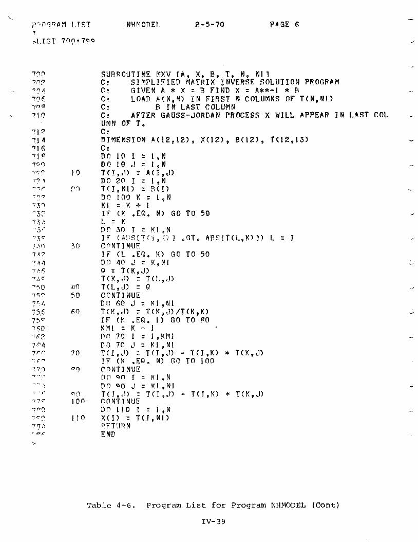
SUEROUTIYE MXV E A , X, B , , T 9 N, AS1 3 C : S I Y P L I F P E D VPTRIX INVERSE SOLUTION PRBGRhM C: GIVEN A * X = E F I N D X = A + * - 1 * R C: LOPD A ( M , f l ) I N F I R S T N COLUMNS OF T ( N 9 M 1 9 C: 8 I N LAST COLffMM C: hFTER G R O S S - J O R D A N PROCESS X & I L L BPPEAR I N LAST COL UMW O f T, Ct DIMENSION 8(82,12) , X ( 1 2 9 , 8(12), T(12,13) C: DC! 10 I = l p M D C 10 J = I , # T ( f , c ' ) = A ( P 9 J 9 D C 2 Q I = l , N T(ITN1> = B ( I ) D n 109 K = 1 , R t K 1 = K + 1 I F ( K .EQ, M I GO TO 50 L = K Df 38 I = K f ,N J F (AFSiTfl,':) I .GT, AE?SIT(E,K) 3 ) L = I CPNTIMUE I F (L . E Q . K) G O TO 50 DI! 40 L! = K , N 1 8 = T ( K , J ) TCK,cl> = T ( L , J > T ( L , J > = O CCNTI NUE D O 60 J = K1 , N l K t = T ( K 9 J ) / T ( K 9 K > I F (K .EQ. I ) G O TO PO K Y I = K - 1 P O 70 I = I , K M I D O 70 J = K 1 , N l T ( I , , l > = T ( I , J ) - f ( I , K ) * T ( K , J ) I F (K . E n , N ) G(! T O 1100 C n N T I N U E rm on r = K I , N n9 Q Q J = K 1 , N l T ( 1 9 t 1 ) = T ( I p r l ) - T ( J , K ) * T ( K , J ) Cl?WTf lVUE D n 110 I = 1 9 N X ( Z ) = T ( X , N l ) PF'T'lPP! E lrdO
Tablc 4 - 6 . Program List for Program NMMODEL (Cont)
IV- 39
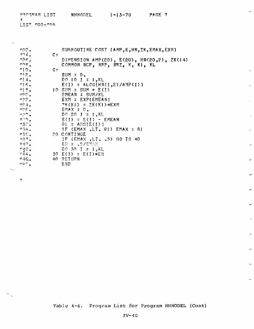
Pnn.7Rb M L I S T NHMODEL 1-13-70 P h G E 7 t L I S T f ? O Q r u Q Q
SUBROUTINE COST IAVP,E,HN,ZK9EMAXoEXMl C,
DSPENSZON AWP(20), E(20) WN(20,2), ZK(14) COMMON NCP, NRP, NRZ, K, K 1 , KL
C ? SUE = 0. D O 10 I = 1,KL E ( I ) = A L P G [ H N ( 1 9 2 ) / A ! 4 P ( I ) I
19 SUM = SUP + E ( 1 ) EWEAN = SUM/KL EXM = EXP[EMEANI 7Y(KI) = ZK(Kl)*EXM EWbX = 0, Dn 20 1 = 1 ,K1. E ( 1 ) = E(I> - E M E A N 01 = A9SfE(I>l I F ( E M A X .LT, 81) E M A X = Q 1
?O C C M T I N U E IF ( E M A X o L T e e 5 ) G O TO 40 E;: = . S / E " r ' > i D P 30 I = I , K L
30 E(I> = E(I>*ER 4C1 3ETLJRN
END
Table 4-6. Program List for Program NHMODEL (Con t )
f V - 4 0
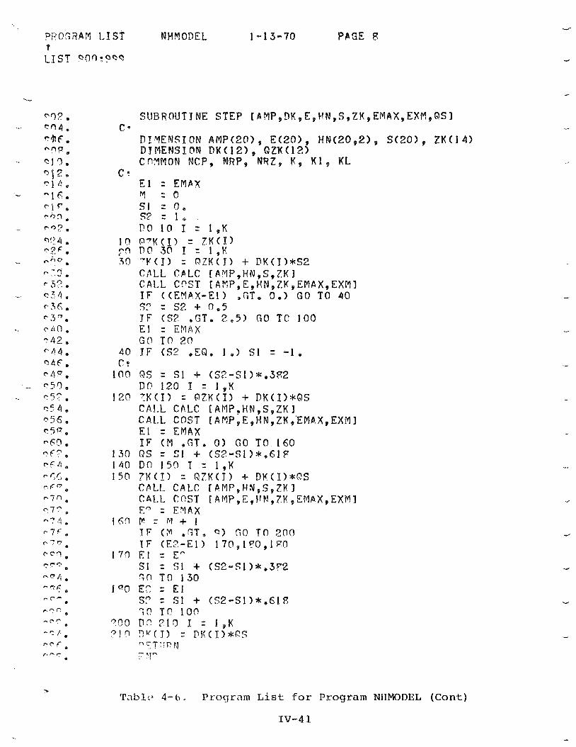
PPO32AM LIST NHMODEL 1 - 1 3-70 PhGE Fc t LIST Qnn:ycc
S U B R O U T I N E STEP [ f i M P , D ~ , E , H N , S P Z K 9 E M A X , E X f v f B Q S I C e
DIPdEWSXON AMP(201, E(20), HN(Z?09Z), S(20>, ZK(14) DIMENSION DK(121, QPK(12) C9?lVIMON NCP, NRP9 NRZ, K, Kl, KL
C ? E l = EPICIY Y = r , SI = Q, 52 = l 8 1?0 10 I = l , K
I n P-K(I) = ZK(X) Fn DO 30 I = 1 , K 30 Y ( I ) = f lZK(I) + DK(I)*SZ
CALL. C P L C [AYP,HN,S,ZKI CA1.L CCST IAKP,E,HN,ZK,EMAX,EXMI TF ((EMAX-Ei) .GT. 0.1 G O TO 40 S ? Z SS3. + 0 , 5 I F (SP a G T e 2 e 5 ) G O TO 100 El = E M A X GI! Tc' 20
40 SF (S2 .EQ. 1 .) S1 = - 1 c :
Ion QS = SI + (s~-sI)*,~Rz DD 120 1 = 1 * K
120 :K(I) = B7K(I) + DK(I)*BS CAI-L CPL.C [AMP,HN,S,ZKI C A L L COST [ANP9E9NN,ZK,EMAX,EXM3 E l = EMAX IF ( M .GT. 0) G O T O 160
1.30 QS = Sl + (S2-S1)*,61P 140 D O 159 I = l,K 150 7 K ( I ) = QZK(T) + DF(I)*OS
C P L L CALG IAMP,HM,S,ZK I CALL C f l S T IAMP,E,lIN,7K,EMAX9EXM1 Eq = E Y A X
160 P r Y + 1 IF (P I .GT, Q ) G O T O 200 I F ( E ? - E l ) 170,1?091R0
1 7 0 El - E" S1 = S1 + (S2-S1)*,3F2 "I T O 130
J V O E" = EI S> S l + (SZ-Sl)*,Glg 12 T O 100
I ZqO P 2 7 1 3 I = 1,K ? W ( T ) = DK(S)*QS '''TIir'PJ f 'i!" . I
Tabl : . 4 - 6 . Program L i s t f a r Program NIIMODEL ( C o n t )
4,5 THE PSEUDOINVERSE
Kinkel 1 2 a 1 has developed an e f f i c i e n t a lgor i thm f o r computing
t h e pseudoinverse of a matr ix which can s impl i fy t h e s o l u t i o n
o f eqn. (4 -32 ) .
The weighted l e a s t squares s o l u t i o n f o r - X using t h e pseudoinverse
is represented a s follow^:
Even i f A i s poorly condi t ioned so t h a t it cannot be inver t ed ,
t h e weighted l e a s t squares s o l u t i o n of - X i s given by eqn. (4-42).
The use of t h e pseudoinverse w i l l avoid t h e i t e r a t i v e method
assoc ia ted with eqn. ( 4 - 3 3 ) .
SECTION V
HORI ZONTAL PROCESSING
5.0 INTRODUCTION
P r e s e n t methods f o r r o u t i n e t o p s i d e ionogram d a t a r e d u c t i o n
depend on t h e fo l lowing s i m p l i f y i n g assumptions:
a . V e r t i c a l p ropaga t ion of t h e echo p u l s e
b. S p h e r i c a l l y s t r a t i f i e d ionosphere o v e r t h e pe r iod o f t h e
X-Trace
I t is a b a s i c p rope r ty of t h e t o p s i d e sounding s a t e l l i t e s u s ing
swept frequency r a d a r t echniques t h a t s u c c e s s i v e h ' ( f ) echo
p u l s e s correspond t o i onosphe r i c soundings a t d i f f e r e n t e a r t h -
based coo rd ina t e s . I t i s w e l l known t h a t t h e ionosphere is
nonsphe r i ca l ly s t r a t i f i e d 'lbl and s i n c e t h e A l o u e t t e 11 s a t e l l i t e
moves a t an average v e l o c i t y of approximately 7 km/sec t h e
e f f e c t s o f h o r i z o n t a l g r a d i e n t s i n t h e o r b i t a l p l ane should be
taken i n t o c o n s i d e r a t i o n .
P T C S C I I ~ i ~ i l c ~ g r i ~ t i i d a t a s-oduction methods f o r h' ( f ) -+ l\l (h)
compu ta t i o~ l i ~ s s u t ~ ~ t ~ ' 2 constank C I c ~ t r o n d e n s i t y prof i le f o r t h e
ionosphere dusirlcj the pe r iod of u s e f u l d a t a a c q u i s i t i o n i n each
ionogram. I n a d d i t i o n , t h e Forward, I n v e r s e , and Matr ix p roces s ing
methods a rc cancer-ncd v i t h reduc ing t h e d a t a from only one
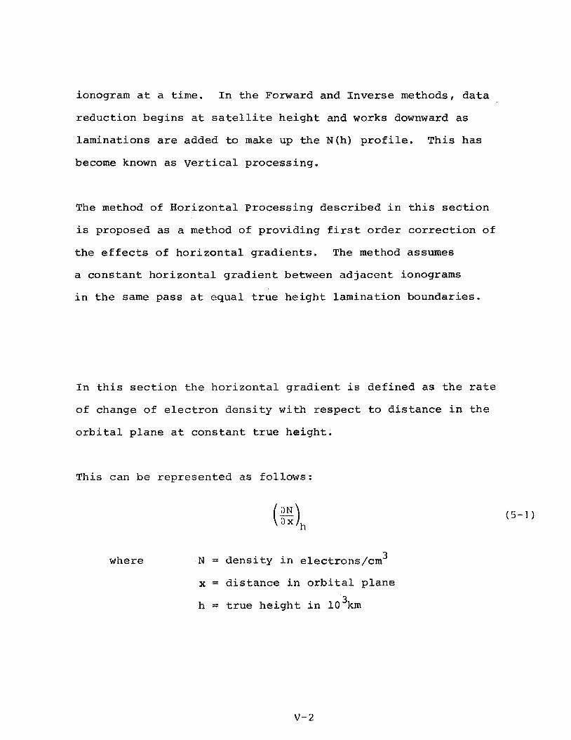
ionogram a t a t i m e . I n t h e Forward and I n v e r s e methods, d a t a
r e d u c t i o n beg ins a t s a t e l l i t e h e i g h t and works downward a s
l amina t ions a r e added t o make up t h e N(h) p r o f i l e . T h i s has
become known as v e r t i c a l p roces s ing .
The method of Hor i zon ta l P roces s ing d e s c r i b e d i n t h i s s e c t i o n
is proposed a s a method of p rov id ing f i r s t o r d e r c o r r e c t i o n o f
t h e e f f e c t s o f h o r i z o n t a l g r a d i e n t s . The method assumes
a c o n s t a n t h o r i z o n t a l g r a d i e n t between a d j a c e n t ionograrns
i n t h e same pas s a t e q u a l t r u e h e i g h t l amina t ion boundar ies .
I n t h i s s e c t i o n t h e h o r i z o n t a l g r a d i e n t i s de f ined as t h e r a t e
o f change of e l e c t r o n d e n s i t y w i t h r e s p e c t t o d i s t a n c e i n t h e
o r b i t a l p l a n e a t c o n s t a n t t r u e h e i g h t ,
This can be r e p r e s e n t e d as fo l lows:
where N = d e n s i t y i n e lec t rons /cm 3
x = d i s t a n c e i n o r b i t a l p l a n e
3 h = t r u e h e i g h t i n 10 km
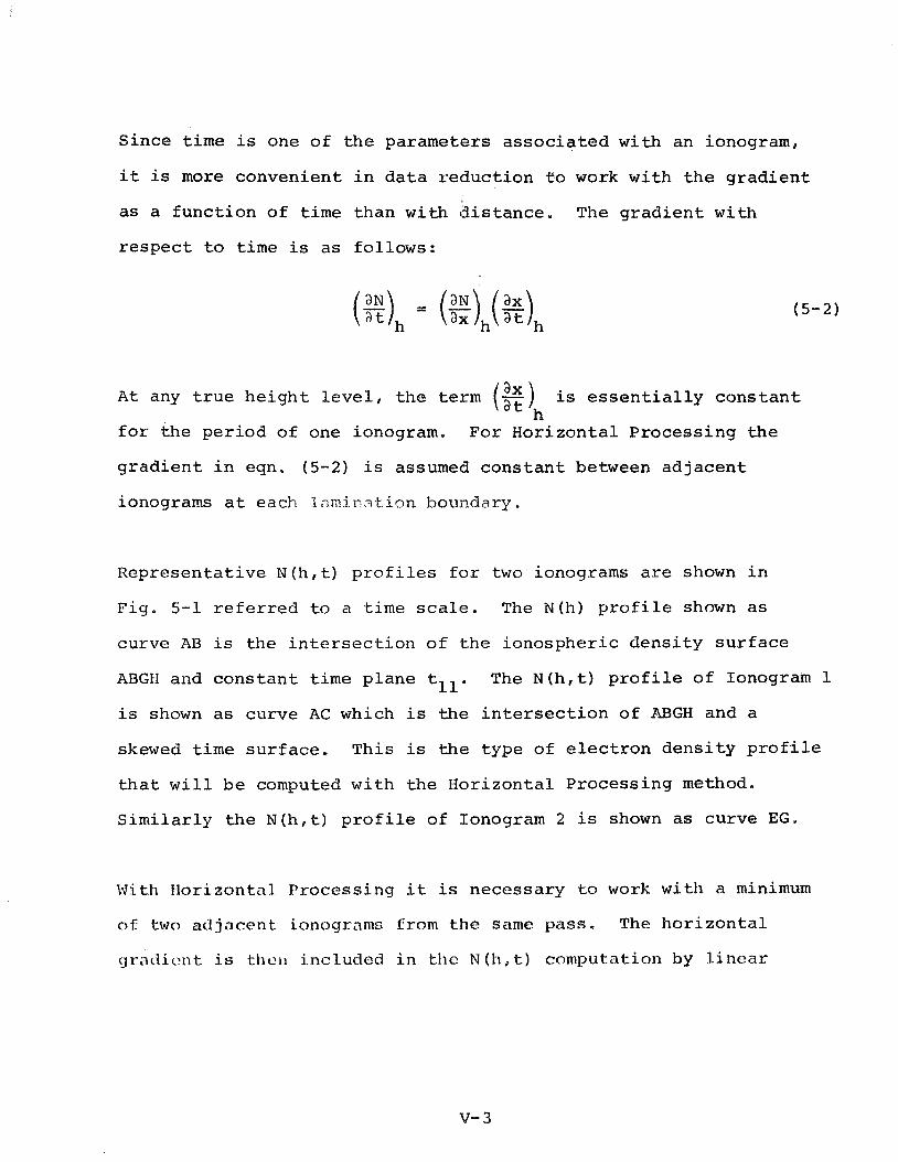
Since t i m e i s one of t h e parameters a s s o c i a t e d wi th an ionogram,
it is more convenien t i n d a t a r e d u c t i o n t o work w i t h t h e g r a d i e n t
as a f u n c t i o n o f t i m e t han w i t h d i s t a n c e . The g r a d i e n t w i th
r e s p e c t t o t i m e is a s fo l lows:
A t any t r u e h e i g h t l e v e l , t h e t e r m (g)h is e s s e n t i a l l y c o n s t a n t
f o r t h e p e r i o d o f one ionogram. For Hor i zon ta l P roces s ing t h e
g r a d i e n t i n eqn. (5-2) i s assumed c o n s t a n t between a d j a c e n t
ionograms a t eacb I a m i r . ~ t i o n boundary.
Represen ta t ive N ( h , t) p r o f i l e s f o r two ionograms a r e shown i n
F ig . 5-1 r e f e r r e d t o a t i m e s c a l e , The N (h ) p r o f i l e shown a s
curve AB is t h e i n t e r s e c t i o n of t h e i onosphe r i c d e n s i t y s u r f a c e
ABGB and c o n s t a n t t i m e p l ane tll. The N ( h , t ) p r o f i l e o f Ionogram 1
i s shown a s curve AC which is t h e i n t e r s e c t i o n of ABGH and a
skewed t i m e s u r f a c e . This i s t h e t ype of e l e c t r o n d e n s i t y p r o f i l e
t h a t w i l l b e computed w i t h t h e Hor i zon ta l P roces s ing method.
S i m i l a r l y t h e N ( h , t ) p r o f i l e of Ionogram 2 i s shown as curve EG.
Wi th Hor i zon ta l P roces s ing it is necessary t o work wi th a minimum
of two a d j a c e n t ionogramc from t h e same pass. The h o r i z o n t a l
~ j rac l ic~nt i s thcil i ncluded i n tile N (11, t) computation by l i n e a r
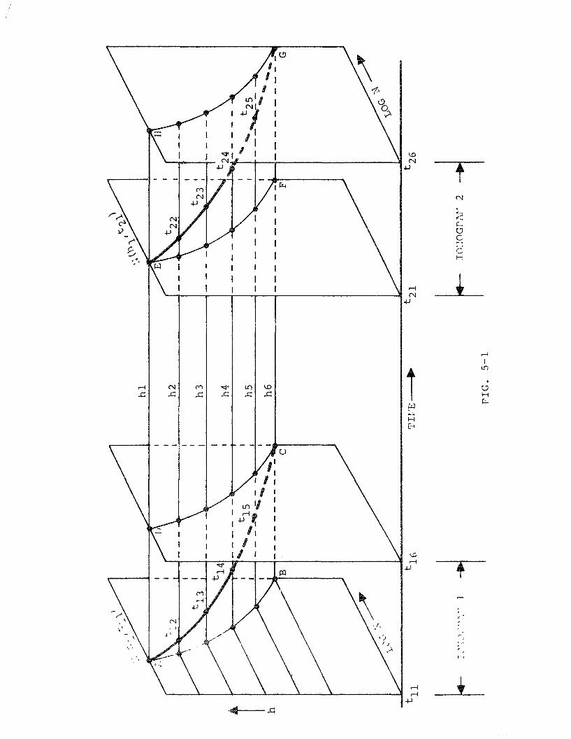
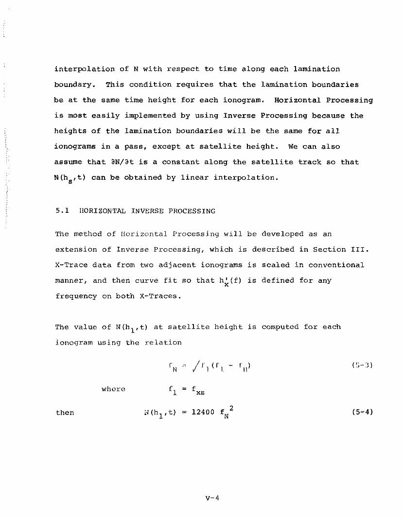
i n t e r p o l a t i o n of N w i t h r e s p e c t t o t i m e a long each l amina t ion
boundary. This c o n d i t i o n r e q u i r e s t h a t t h e l amina t ion boundar ies
be a t t h e same t i m e h e i g h t f o r each ionogram. Hor i zon ta l P roces s ing
i s m o s t e a s i l y implemented by u s i n g I n v e r s e Process ing because t h e
h e i g h t s o f t h e l amina t ion boundar ies w i l l be t h e same f o r a l l
ionograms i n a pas s , excep t a t sa te l l i te h e i g h t . W e c an also
assume t h a t %?/at is a c o n s t a n t a long t h e sa te l l i te t r a c k s o t h a t
W (hs, t ) can b e ob ta ined by l i n e a r i n t e r p o l a t i o n .
5 . 1 IIORIZONTAL INVERSE PROCESSING
The method of 13orizontal Process iny w i l l b e developed a s an
ex t ens ion of Inve r se Process ing , which is d e s c r i b e d i n S e c t i o n 111.
X-Trace d a t a from t w o a d j a c e n t ionograms i s s c a l e d i n convent iona l
manner, and then curve f i t s o t h a t h i ( f ) i s de f ined f o r any
frequency on bo th X-Traces,
The va lue o f N ( h l , t ) a t s a t e l l i t e h e i g h t is computed for each
ionogram us ing t h e r e l a t i o n
where
then
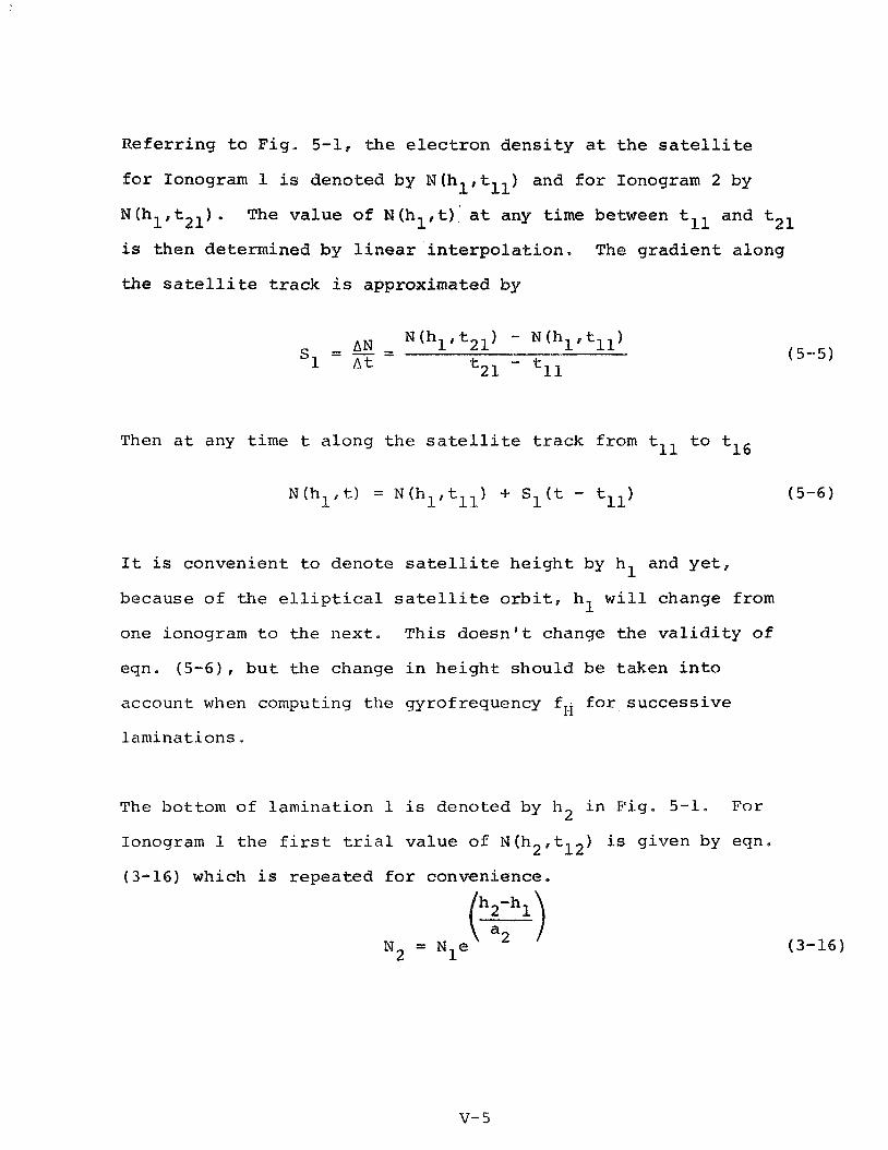
Refe r r ing t o F ig , 5-1, t h e e l e c t r o n d e n s i t y a t t h e s a t e l l i t e
f o r Ionogram 1 is denoted by N(hl.tll) and f o r Ionogram 2 by
N (hl , tll) . The v a l u e o f N (hl, t) a t any t i m e between tll and t21
is then determined by l i n e a r i n t e r p o l a t i o n . The g r a d i e n t a long
t h e s a t e l l i t e t r a c k i s approximated by
Then a t any t i m e t a long t h e s a t e l l i t e t r a c k from tll '16
I t is convenien t t o denote s a t e l l i t e h e i g h t by hl and y e t ,
because of t h e e l l i p t i c a l s a t e l l i t e o r b i t , hl w i l l change from
one ionogram t o t h e nex t . This d o e s n ' t change t h e v a l i d i t y o f
eqn. (5-6) , b u t t h e change i n h e i g h t should be taken i n t o
account when computing t h e gyrofrequency fIi f o r s u c c e s s i v e
l amina t ions .
The bottom of l amina t ion 1 is denoted by h2 i n F ig . 5-1. For
Ionogram 1 t h e f i r s t t r i a l va lue of N(h2,t12) is g iven by eqn.
(3-16) which i s r epea t ed f o r convenience.
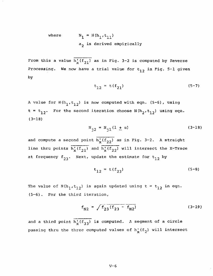
where N1 = N(hlUtll)
a 2 i s d e r i v e d e m p i r i c a l l y
Prom t h i s a va lue h;(f21) as i n F ig . 3-2 is computed by Reverse
Process ing . W e now have a t r i a l va lue f o r t12 i n Fig . 5-1 g iven
by
t12 = t(f21) ( 5 -7 )
A va lue f o r N(hl, t12) i s now computed w i t h eqn. (5 -6) , u s i n g
t = t12. For t h e second i t e r a t i o n choose N(h2,t12) u s ing eqn.
(3-18)
and compute a second p o i n t h & ( f Z 2 ) a s i n F ig . 3-2. A s t r a i g h t
l i n e t h r u p o i n t s hi (f21) and hi ( f 2 2 ) w i l l i n t e r s e c t t h e X-Trace
a t frequency f Z 3 * Next, update t h e e s t i m a t e f o r t12 by
The va lue of N(hl,t12) is aga in updated us ing t = t12 i n eqn.
(5-6) . For t h e t h i r d i t e r a t i o n ,
and a t h i r d p o i n t h k ( f 3 3 ) i s computed. A segment of a circle
pas s ing t h r u t h e t h r e e computed v a l u e s o f h;(f2) w i l l i n t e r s e c t
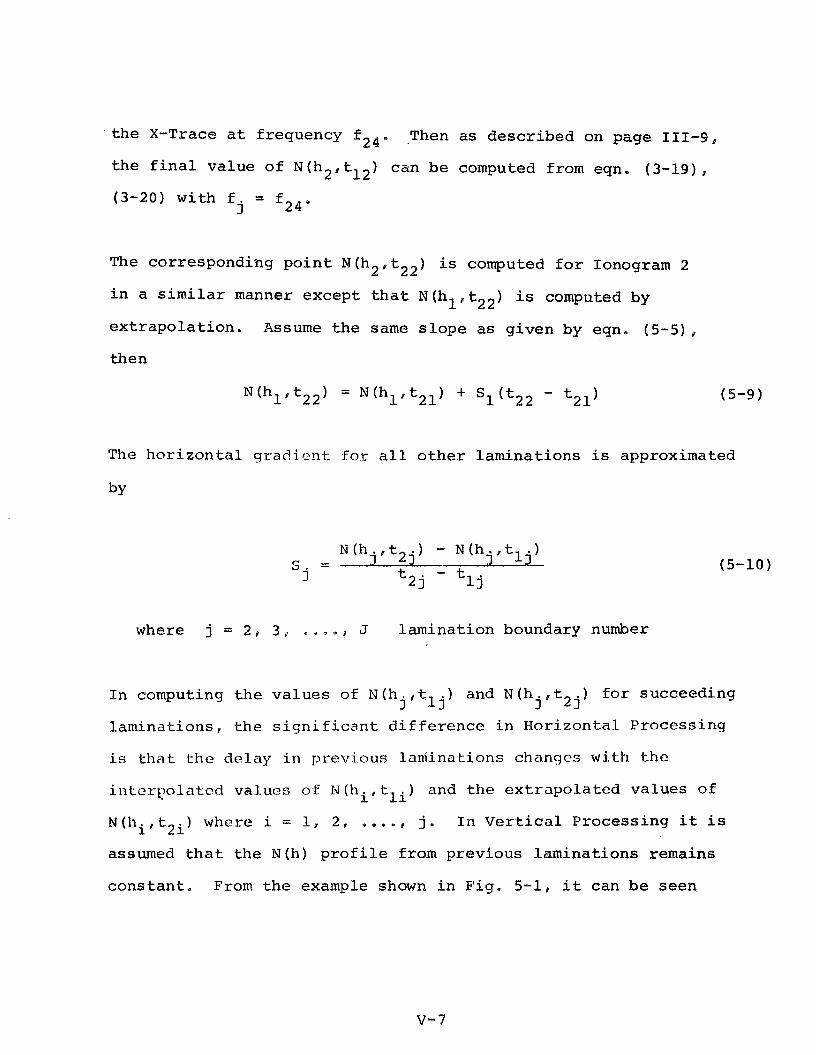
t h e X-Trace a t f requency f Z 4 . Then as d e s c r i b e d on page 111-8,
t h e f i n a l va lue o f N(h2,t12) can be computed from eqn. (3 - IS) ,
(3-20) w i t h f j = f 2 4 .
The cor responding p o i n t N (h2, t22) i s computed f o r Ionogram 2
i n a s imi la r manner excep t t h a t N(hl , tZ2) is computed by
e x t r a p o l a t i o n . Assume t h e same s l o p e as g iven by eqn. (5 -5 ) ,
then
The h o r i z o n t a l g r a d i e n t f o r al-1 o t h e r l amina t ions is approximated
by
where j = 2 3 . J l amina t ion boundary number
I n computing t h e v a l u e s of N (h , -t: . ) and N (h . , t ) f o r succeeding j 11 I 2 j
l amina t ions , t h e s i g n i f i c a n t d i f f e r e n c e i n Hori.zonta1 Process ing
is that t h e delay i n p rev ious l amina t ions changes wi th t h e
interpolated values of N ( h i , tli) and t h e e x t r a p o l a t e d va lues o f
N(hi , tZi) w h e r e i = 1, 2 , ...., j. I n V e r t i c a l P roces s ing it i s
assumed t h a t t h e N ( h ) p r o f i l e from prev ious l amina t ions remains
c o n s t a n t . From t h e example shown i n F i g , 5-1, it can b e seen

t h a t c o r r e c t i o n f o r t h e e f f e c t s of h o r i z o n t a l g r a d i e n t s r e q u i r e s
t h e u se o f e x t r a p o l a t e d d a t a i n Ionogram 2 , wh i l e f o r Ionogram 1
t h e c o r r e c t i o n is o b t a i n e d by i n t e r p o l a t i o n . The use o f
e x t r a p o l a t e d d a t a v a l u e s can be minimized by p roces s ing t h e
ionograms i n a pas s s t a r t i n g wi th t h e l a s t t w o ionograms and
working i n r e v e r s e sequence. A f t e r t h e l a s t two ionograms have
been reduced t h i s way, t h e one r e f e r r e d t o a s Ionogram 1 becomes
t h e i n t e r p o l a t i o n r e f e r e n c e f o r t h e nex t p rev ious ionogram and no
f u r t h e r c x t r a p o l a t i o n i s r e q u i r e d f o r t h e remaining ionograms i n
t h e pass .
The f i n a l o u t p u t N ( h , t ) p r o f i l e i s then p rope r ly t h e i n t e r s e c t i o n
o f t h e i onosphe r i c d e n s i t y s u r f a c e ABGH of F ig . 5-1 and a c o n s t a n t
t ime p lane . I t then i s a matter o f choosing t h e t i m e p l ane i n
each ionogram a t which t o compute M ( h , t ) . I n F ig . 5-1, t h e curve
AB is t h e N ( h , t ) p r o f i l e where tll = t ( f x S ) . One may wish t o
s e l e c t t h e t ime p l ane a t t = t16. This is convenien t i n t h a t t h e
curve DC is a l r e a d y known a t t h e time t h e va lue of N i s corrrputed j
at thr I.owcr bounda ry oC t l l c ? 12s t I am.ina t i nri.
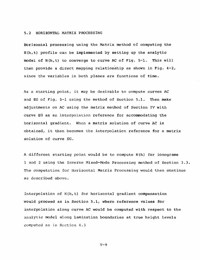
5.2 HORIZONTAL MATRIX PROCESSING
Hor i zon ta l p roces s ing u s i n g t h e Mat r ix method o f computing t h e
M(h , t ) p r o f i l e can be implemented by s e t t i n g up t h e a n a l y t i c
model o f N (h , t) t o converge t o c u r v e AC o f F ig . 5-1. This w i l l
t hen prov ide a d i r e c t mapping r e l a t i o n s h i p as shown i n F ig . 4-2,
s i n c e t h e v a r i a b l e s i n bo th p l a n e s are f u n c t i o n s of t i m e .
A s a s t a r t i n g p o i n t , i t may be d e s i r a b l e t o compute curves AC
and EG o f F ig . 5-1 u s i n g t h e method o f S e c t i o n 5.1. Then make
ad jus tments on AC u s i n g t h e m a t r i x method o f S e c t i o n I V w i t h
c u r v e EG as an i n t e r p o l a t i o n r e f e r e n c e f o r accommodating t h e
h o r i z o n t a l g r a d i e n t . When a m a t r i x s o l u t i o n o f cu rve AC i s
ob ta ined , it then becomes t h e i n t e r p o l a t i o n r e f e r e n c e f o r a m a t r i x
s o l u t i o n o f curve EG.
A d i f f e r e n t s t a r t i n g p o i n t would b e t o compute N(h) f o r ionograms
1 and 2 u s ing t h e I n v e r s e Mixed-Mode P roces s ing method o f S e c t i o n 3 . 3 .
T h e computation f o r Hor i zon ta l Matr ix P roces s ing would t h e n con t inue
a s desc r ibed above.
I n t e r p o l a t i o n of N ( h , t ) f o r h o r i z o n t a l g r a d i e n t compensation
would proceed a s i n S e c t i o n 5 -1 , where r e f e r e n c e v a l u e s for
i n t e r p o l a t i o n a long c u r v e AC would be computed w i t h r e s p e c t t o t h e
a n a l y t i c model a long l amina t ion boundar ies a t t r u e h e i g h t l e v e l s
computed a s i n S e c t i o n 4 . 3
Prepared f o r :
Wstrodata , Znc, 240 EO P a l a i s Rd. Anaheim, C a l i f ,
A s t r o d a t a P r o j e c t 938400
TR- 1
SOME PROPOSED METEIODS FOR W D U C T I O N
O F T O P S I D E IONOGRANS
TO ELECTRON DENSITY P R O F I L E S
September 25# 1949
John F, Kinkel Technica l Consu l t an t Mewport Beach, C a l i f ,
TABLE OF CONTENTS
Abstract
Introduction
Approximation of h ' (f, t)
Approximation of N (h, t)
Conclusion
TR-1 Page 1

TR-1 Page 2
l%bs t ract
Thig paper proposes a method which m y be used t o f i n d an
e l e c t r o n d e n s i t y p r o f i l e y i e l d i n g t h e l e a s t squares e r r o r f i t
t o t h e observat ions. operato& j u d m n t of t h e q u a l i t y of
observat ion is taken i n t o account i n the d a t a reduct ion
process. A method by which time and p o s i t i o n v a r i a t i o n s
occurr ing over t h e observat ion per iod may be cor rec ted for
is a l s o proposed,
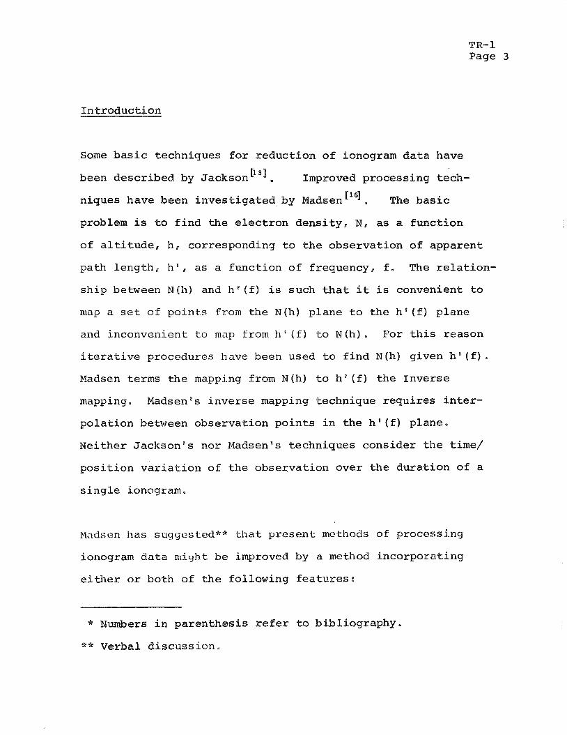
TR-1 Page 3
In t roduc t ion
Some b a s i c techniques f o r reduct ion of ionogram d a t a have
[I31 been descr ibed by Jackson Improved processing tech-
1161 niques have been i n v e s t i g a t e d by Madsen The b a s i c
problem is t o f i n d t h e e l e c t r o n dens i ty , N, as a funct ion
of a l t i t u d e , h , corresponding t o t h e observat ion of apparent
path length , h S , a s a funct ion of frequency, f . The r e l a t i o n -
s h i p between N(h) and h u ( £ ) i s such t h a t it i s convenient t o
map a s e t of po in t s from t h e N(h) plane t o t h e h s ( f ) plane
and inconvenient to map from h ' ( f ) t o N (h ) . For t h i s reason
i t e r a t i v e procedures have been used t o f i n d N(h) given h s ( f ) .
Pladsen terms t h e mapping from N (h) t o h ' ( f ) t h e Inverse
mapping, Madsenss inve r se mapping technique requ i res i n t e r -
po la t ion between observat ion p o i n t s i n t h e h s ( f ) plane,
Nei ther Jackson8s nor Madsen's techniques cons ider t h e time/
p o s i t i o n v a r i a t i o n of t h e observat ion over t h e dura t ion of a
s i n g l e ionogram,
Mndsen h a s suggcstcd** t h a t p resen t methods of processing
ionogram data r n i y h t be improved by a method incorpora t ing
either o r both of t h e following f e a t u r e s :
* Mumbers i n pa ren thes i s r e f e r t o bibl iography.
** Verbal d i scuss ion ,
TR-1 Page 4
1, Time/position v a r i a t i o n over t h e observat ion
period of one ionogram is accounted f o r ,
2, Data from usable por t ions of a l l t h r e e
t r a c e s , Z, 0, and X, from a s i n g l e ionogram a r e used
e f f e c t i v e l y t o genera te t h e N (h) p r o f i l e ,
The balance of t h i s paper desc r ibes proposed methods f o r
accomplishing t h e s e goals . The methods descr ibed f o r
accomplishing items 1 and 2 above a r e e s s e n t i a l l y independent;
i. e., e i t h e r may 1 i4~d without t h e o t h e r ,
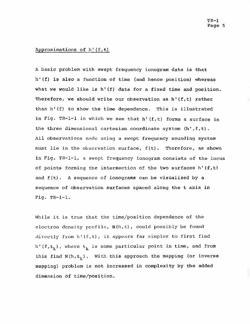
TR-1 Page 5
Approximations o f h 8 ( f , t )
A b a s i c problem w i t h swept frequency ionogram d a t a is t h a t
h g ( f ) i s a l s o a f u n c t i o n o f t i m e (and hence p o s i t i o n ) whereas
what w e would l i k e i s h e ( f ) d a t a f o r a f i x e d t i m e and p o s i t i o n ,
Therefore , w e should w r i t e ou r o b s e r v a t i o n as h ' (f, t) r a t h e r
t han h s ( f ) t o show t h e t i m e dependence. This i s i l l u s t r a t e d
i n F i g , TR-1-1 i n which w e see t h a t h ' ( f , t ) forms a s u r f a c e i n
t h e t h r e e dimensional c a r t e s i a n c o o r d i n a t e system ( h D , f , t ) .
A l l obse rva t ions made u s ing a swept frequency sounding system
must l i e i n t h e observation s u r f a c e , f ( t ) . Therefore , as shown
i n F ig . TR-1-1, a swept f requency ionogram c o n s i s t s o f t h e l ocus
of p o i n t s forming t h e i n t e r s e c t i o n of t h e two s u r f a c e s h s ( f , t )
and f ( t ) . A sequence of ionograms can b e v i s u a l i z e d by a
sequence o f o b s e r v a t i o n s u r f a c e s spaced a long t h e t a x i s i n
F ig . TR-1-1,
While i t i s t r u e t h a t t h e t i m e / p o s i t i o n dependence of t h e
cl .ectron d e n s i t y p r o f i l e , Pa (hc L) , could p o s s i b l y be found
t1ircct l .y f roirt 11 ' ( f , t) , it appears f a r s i rnpler t o f i r s t f i n d
11' ( f . t k ) , where t i s some p a r t i c u l a r p o i n t i n t i m e , and from k
t h i s f i n d N ( h , t k ) . With t h i s approach t h e mapping ( o r i n v e r s e
mapping) problem i s n o t i n c r e a s e d i n complexity by t h e added
dimension of t ime /pos i t i on ,
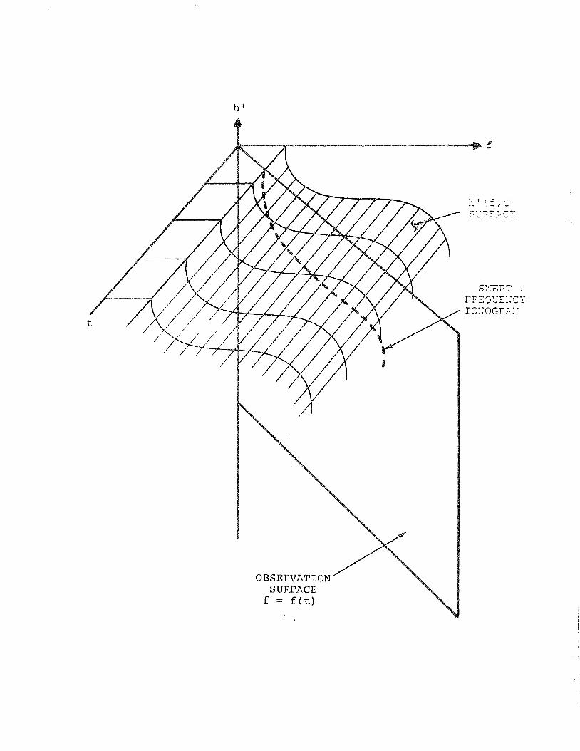
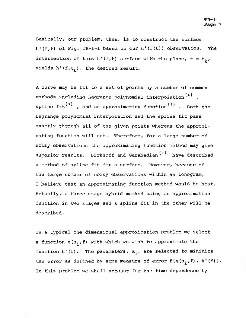
TR-1 Page 7
B a s i c a l l y , o u r problem, t hen , i s t o c o n s t r u c t t h e s u r f a c e
h f ( f , t) o f F ig . TR-1-1 based on o u r h ' ( f (t) ) o b s e r v a t i o n , The
i n t e r s e c t i o n o f t h i s h 8 ( f , t ) s u r f a c e w i t h t h e p l ane , t = tk,
y i e l d s h 8 ( f , tk) , t h e d e s i r e d r e s u l t .
A curve may be f i t t o a s e t o f p o i n t s by a number o f common
methods i n c l u d i n g Lagrange pol$nomial i n t e r p o l a t i o n ( 6 )
s p l i n e f i t ( ) , and an approximating f u n c t i o n ()I ~ 0 t h the
Lagrange polynomial i n t e r p o l a t i o n and t h e s p l i n e f i t pa s s
e x a c t l y through a l l of t h e g iven p o i n t s whereas t h e approxi-
mating f u n c t i o n will n o t . Therefore , f o r a l a r g e number o f
no isy obse rva t ions t h e approxirnating f u n c t i o n method may g i v e
s u p e r i o r r e s u l t s , Birkhoff and Garabedian have d e s c r i b e d
a method o f s p l i n e f i t f o r a s u r f a c e . However, because o f
t h e l a r g e number o f no isy obseyva t ions w i t h i n an ionogram,
I b e l i e v e t h a t an approximating func t ion method would be b e s t .
Ac tua l ly , a t h r e e s t a g e hybr id method us ing an approximation
f u n c t i o n i n two s t a g e s and a s p l i n e f i t i n t h e o t h e r w i l l be
desc r ibed ,
I n a t y p i c a l one dimensional approximat ion problem we select
a fu i lc t ion g ( a i , f ) w i t h which w e wish t o approximate t h e
f u n c t i o n h ' ( f ) . The parameters , ai, a r e s e l e c t e d t o minimize
t h e e r r o r as de f ined by some measure o f e r r o r ~ { g ( a ~ , f ) , h ' ( 5 ) 1 .
11) this problem wc s h a l l account f o r the t i m e dependence by
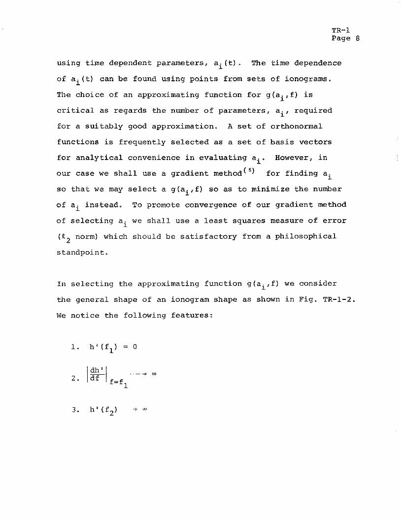
TR-1 Page 8
using time dependent parameters, a i ( t ) . The time dependence
can be found using po in t s from s e t s of ionograms . The choice of an approximating funct ion f o r g ( a i , f ) i s
c r i t i c a l a s regards t h e number o f parameters, ai , requi red
f o r a s u i t a b l y good approximation, A set of orthonormal
funct ions i s f requen t ly s e l e c t e d as a s e t of b a s i s vec to r s
f o r a n a l y t i c a l convenience i n eva lua t ing ai. However, i n
our case w e s h a l l use a g rad ien t method(5) f o r f ind ing ai
s o t h a t we may s e l e c t a g ( a i , f ) s o a s t o minimize t h e number
of ai ins t ead . To promote convergence of our g rad ien t method
of s e l e c t i n g ai we s h a l l use a l e a s t squares measure of e r r o r
(5 norm) which should be s a t i s f a c t o r y from a phi losophica l
I n s e l e c t i n g t h e approximating funct ion g ( a i , f ) we consider
t h e genera l shape of an ionogram shape a s shown i n Fig. TR-1-2.
We n o t i c e t h e fol lowing f e a t u r e s :
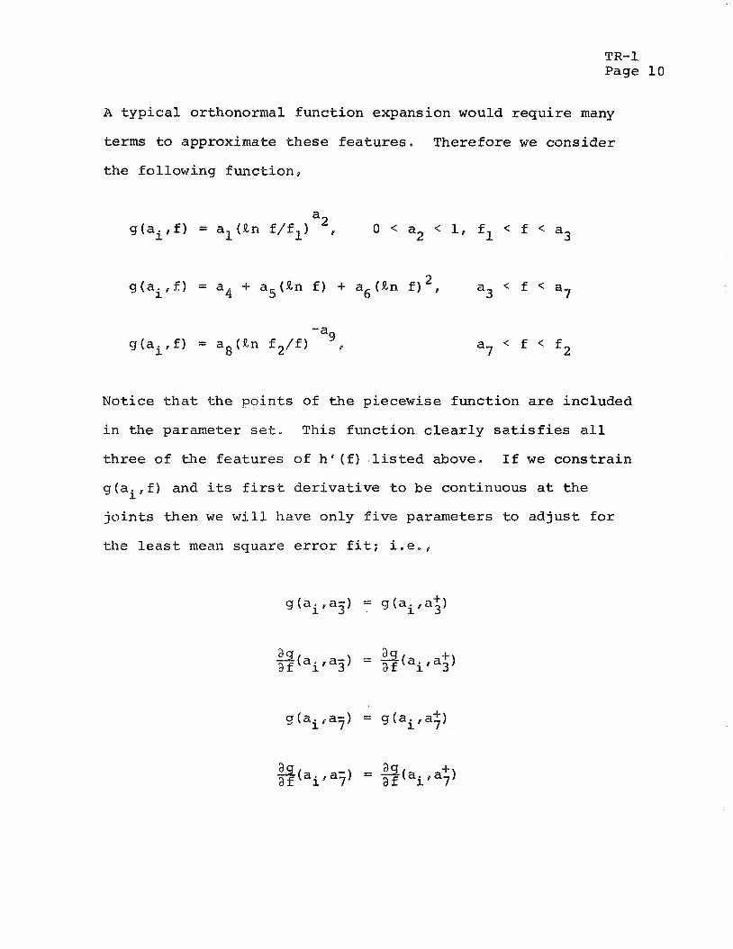
TR-1 Page 10
A t y p i c a l orthonormal funct ion expansion would r e q u i r e many
terms t o approximate these f e a t u r e s . Therefore w e cons ider
t h e fol lowing func t ion ,
Notice t h a t t h e po in t s of t h e piecewise funct ion a r e included
i n the parameter se t . This funct ion c l e a r l y s a t i s f i e s a l l
t h r e e of t h e f e a t u r e s of h a ( f ) l i s t e d above* I f w e c o n s t r a i n
g ( a i f f ) and i t s f i r s t d e r i v a t i v e t o be continuous a t t h e
j o i n t s then we w i l l have only f i v e parameters t o a d j u s t f o r
the l e a s t mean square e r r o r f i t ; i, e , ,
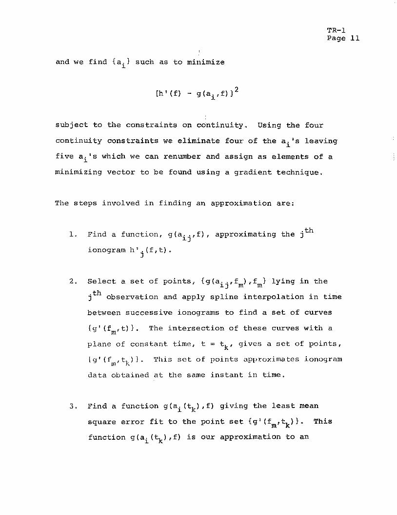
TR- 1 Page 11
and w e f i n d {ai} such as t o rni~iimize
s u b j e c t t o t h e c o n s t r a i n t s on c d n t i n u i t y s Using t h e f o u r
c o n t i n u i t y c o n s t r a i n t s w e e l i m i n a t e f o u r o f t h e ai ' s l e a v i n g
f i v e a i 8 s which w e can renumber and a s s i g n as e lements o f a
minimizing v e c t o r t o b e found u s i n g a g r a d i e n t t echnique ,
The s t e p s involved i n f i n d i n g an approximation a r e :
1. Find a f u n c t i o n , g (ai j, f) , approximating t h e j t h
ionogram h ' ( f , t ) . j
2. S e l e c t a se t of p o i n t s , { g ( a i j , fm) , fm} l y i n g i n t h e
jth o b s e r v a t i o n and apply s p l i n e i n t e r p o l a t i o n i n t i m e
between s u c c e s s i v e ionograms t o f i n d a set o f curves
{gv ( fm. t) 1 . The i n t e r s e c t i o n o f t h e s e curves w i t h a
p l a n e of c o n s t a n t t ime, t = tk, g i v e s a s e t of p o i n t s ,
( g ' ( f,, tk) 1 - T h i s sct of point:; op~)ronima tcs ionogrom
d a t a o b t a i n e d a t t h e same i n s t a n t i n t i m e .
3 . Find a f u n c t i o n g (ai (tk) , f ) g i v i n g t h e l e a s t mean
s q u a r e e r r o r f i t t o t h e p o i n t set { g ' ( f m , % ) } . T h i s
f u n c t i o n CJ (ai (tk) f ) i s o u r approximation t o an
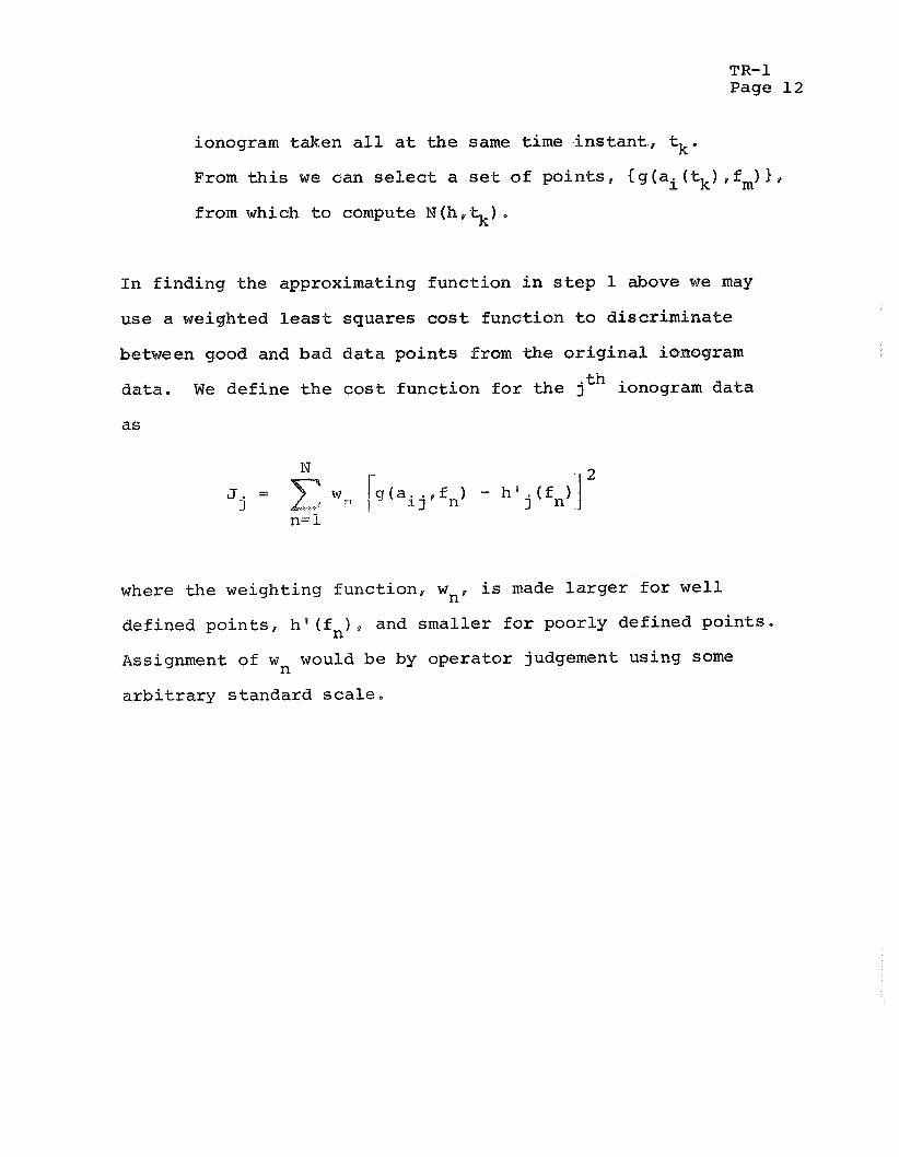
TR-1 Page 12
ionogram taken a l l a t t h e same time i n s t a n t , tk.
From t h i s w e can s e l e c t a set of p o i n t s , { g (ai (tk) , fm) 1 ,
from which t o compute M (la,\) .
I n f ind ing t h e approximating funct ion i n s t e p 1 above w e may
use a weighted least squares cos t funct ion t o d i sc r imina te
between good and bad d a t a p o i n t s from the o r i g i n a l ienogram
data . W e de f ine t h e c o s t funct ion f o r t h e jth ionogram d a t a
a s
where t h e weighting funct ion , wn, i s made l a r g e r f o r w e l l
def ined p o i n t s , h ' ( f , ) , and smal ler f o r poorly def ined po in t s .
Assignment of wn would be by opera to r judgement using some
a r b i t r a r y s tandard s c a l e ,
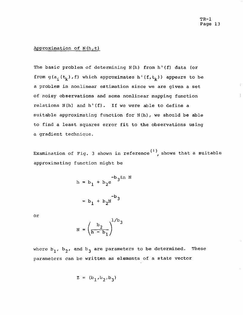
TR- 1 Page 13
Approximation of N (h , t)
The b a s i c problem of determining M(h) from h o (f) d a t a ( o r
from g ( a i ( t k ) , f ) which approximates h 8 ( f , t k ) ) appears t o be
a problem i n nonl inear es t imat ion s i n c e we a r e given a s e t
of noisy observat ions and some nonl inear mapping funct ion
r e l a t i o n s N (h) and h ' ( f ) , I f we were a b l e t o d e f i n e a
s u i t a b l e approximating funct ion f o r M(h), we should be a b l e
t o f i n d a l e a s t squares e r r o r f i t t o t h e observat ions using
a g r a d i e n t technique,
) shows t h a t a s u i t a b l e Examination of Fig. 3 shown i n r e fe rence
approximating funct ion might be
whore bl , b2, and b3 a r e parameters t o be determined. These
paramletcrs can be w r i t t e n as elements of a s t a t e vec to r
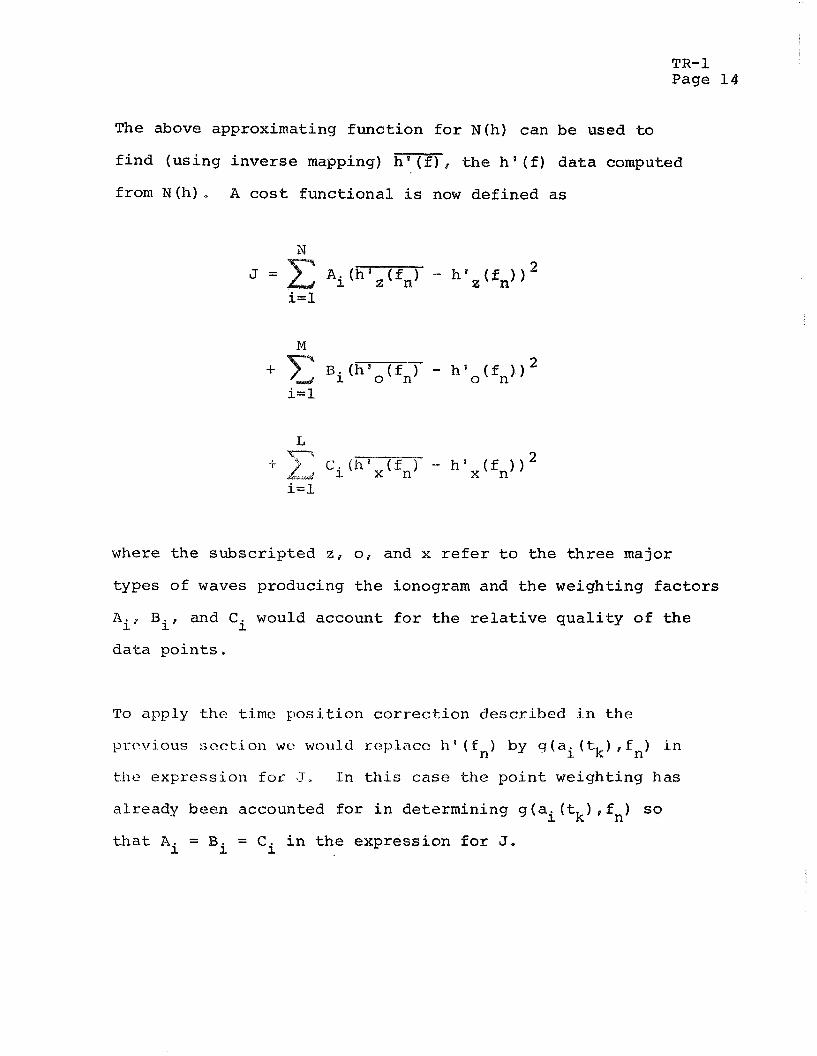
TR- 1 Page 1 4
The above approximating funct ion f o r N(h) can be used t o
f i n d (us ing inver se mapping) h g (f) , t h e h ' ( f ) d a t a computed
from N(h) . A c o s t func t iona l i s now def ined as
where t h e subsc r ip ted z , o r and x r e f e r t o t h e t h r e e major
types of waves producing t h e ionogram and t h e weighting f a c t o r s
Ait B i t and Ci would account f o r t h e r e l a t i v e q u a l i t y of t h e
d a t a p o i n t s .
To app ly t h e time p o s i t i o n c o r r e c t i o n descr ibed i n the
the expression fcjr J, In this case t h e po in t weighting has
already been accounted f o r i n determining g ( a i ( t k ) , f n ) 50
t h a t Ai = Bi = Ci i n t h e expression f o r J.
TR- 1 Page 1 5
A g r a d i e n t t echnique ( 5 , can now be usea t o determine t h e
s t a t e v e c t o r
such a s t o minimize t h e c o s t f u n c t i o n , J, Therefore , w e
w i l l have determined a l e a s t mean squa re e r r o r f i t of our
approximating f u n c t i o n , N (h ) , t o t h e bbse rva t ions , h " £ 1 , or N ( h , t k ) u s i n g g ( a i ( t k ) , f ) .
TR-1 :
Page 1 6
Conclusion
Methods have been descr ibed f o r f ind ing N(h) o r P ( h , t k ) from
ionograms using approximation theory. A g r a d i e n t technique
i s proposed t o f i n d t h e parameters of t h e approximating
funct ion , The success of t h e technique w i l l depend upan t h e
following f a c t o r s :
1. The appropr ia t e s e l e c t i o n of t h e approximating model.
2 , The speed of convergence of t h e g r a d i e n t method
computation of approximation model parameters.
The approximation model proposed f o r N(h) i s q u i t e simple and
when used w i t h h v ( f ) d a t a would l ead t o r e s u l t s which could
be compared d i r e c t l y with p r e s e n t N (h) r e s u l t s , Therefore, I
recommend t h a t t h i s por t ion of t h e proposed method be evaluated
f i r s t . Since t h e proposed model i s s o simple an a d d i t i o n a l
term involving two a d d i t i o n a l parameters would n o t impose a
computational hardship i f experiments i n d i c a t e a more accura te
model i s requ i red ,
"ipproximating h ' ( f , tk) by g (ai ( tk) . f) appears t o be a more
d i f f i c u l t probl.em s i n c c es t ima t ion i n two dimensions, frequency

TR-1 Page 1 7
and time, is requ i red , Also t h e form of t h e approximating
funct ion appears t o be more complex than f o r N(h) . Another
f a c t o r i s t h a t r e s u l t s obtained by accounting f o r t h e
time/displacement changes over a s i n g l e ionogram could n o t
be compared d i r e c t l y wi th r e s u l t s obtained by c u r r e n t
methods. For t h e s e reasons I recommend t h a t t h e approxi-
mation of h ' ( f , tk) be attempted as a second s t e p following
t h e approximation of N (h) ,
TR-1 Page 18
( J. E . Jackson, "The Reduction of ~ o p s i d e Ionograms t o
E l e c t r o n Densi ty P r o f i l e s " , IEEE Proceedings , V o l . 57#
N o , 6 ( June 1969) pp, 960-975-
( R. G. Madsen, " I s i s Topside Sounder D a t a P rocessor" ,
Study Report No, 93840, As t roda t a , I n c ,
J. R. R i c e , ---.-,- TRc .Approximation * - of Func t ions , Vol. I,
Addison 'Wesley, 1964,
G. Birkhoff and H. L. Garabedian, "Smooth Su r face
I n t e r p o l a t i o n " ,
") J. F. Kinkel , "A Gradien t Method with Improved
Convergence", 9 September 1969.
( 6, R. W. H a m m i n g . Numerical Methods f o r Engineers and
S c i e n t i s t s , McGraw-Hill, 1962,

P r e p a r e d f o r :
A s t r o d a t a , I nc . 240 E . P a l a i s Rd, Anaheim, C a l i f .
A s t r o d a t a P r o j e c t 938400
TR- 2
A WEIGIITELI 1,LfiS'i' SQUAItES APPI?OXIMATION METHOD
November 2 1 , 1969
John F. K i n k e l T e c h n i c a l C o n s u l t a n t N e w p o r t Beach, C a l i f ,
TR- 2 Page l
A WEIGHTED LEAST SQUARES
APPROXI8IATION METHOD*
Given a f u n c t i o n f ( x ) i n t e r m s o f a set o f d a t a p o i n t s {xi , f ( X i ) 1 ,
i = 1 , . - 1 w e wish t o approx imate f ( x ) by t h e f u n c t i o n
F ( X , 2) , 2 = ( a l p . .. . . a K ) T where - u i s a pa ramete r se t which w e
w i l l s e l e c t t o minimize t h e we igh ted mean s q u a r e e r r o r o f t h e
approx imat ion , W e approximate t h e d i f f e r e n t i a l o f F ( X , - a) a t
al?(xit - a ) where V, F(Xir - a) = I ' * . . I -
-
Nc w o u l d l i k e t o f i n d t h e AF such t h a t
( x ) - ( i ' - ( 1 ) - A F ( ) ; ~ , - t x ) = 0 , i = 1, .-.. , N 1
LP t 1 ( t ~ ) = 1- (Xi) - F ( X . , (1) , i = 1, ...., N 1 ' - 1. -
Now w e w i s l l t o f i n d t h e A a - which w i l l p roduce t h i s r e s u l t , W e
have
*A, J. M a l l i n c k r o d t , "A Weighted Leas t -Squares Adjus tment f o r Network S y n t h e s i s " A s t r o d a t a T e c h n i c a l R e p o r t , J u l y 1 9 6 4 .
TR- 2 Page 2
and t h e weighted l e a s t mean square e s t i m a t e f o r Aa i s -
-1 T A c t * = ( A ~ Q A ) h Qy --
where Q i s a symmetric p o s i t i v e d e f i n i t e N x N m a t r i x . Now w e
i t e r a t e on a produc ing s e q u e n t i a l l y -
W e c o n t i n u e i t e r a t i n g on a u n t i l -
Now wc. i r ~ q u i r -cx , I : : I o C i i < . (11-1-or c:ri t c k r i n i mpo:;c.d on e by t h i s -
11lt.- 1 I l O < i s W ( > 1 1 0 P t 11'1 t
TR-2 Page 3
k = 1, ...., K Now consider the cost functional defined by
TR- 2 Page 4
We s e e t h a t
T w e have Aa* = 0 - - ( V J) = 0 ---> min J - a - - a
There fo re , by i t e r a t i n g on a u n t i l we have achieved Aa* = 0 w e - - have a c t u a l l y ach lc i#es cl weighted l e a s t squa re s f i t t o f ( x ) by
F ( X , - a ) , The d e s i r e d r e s u l t i s achieved by sneaking i n through
t h e back door.
1Qe s e e a l s o t h a t i f J were q u a d r a t i c i n a then F would be l i n e a r -
i n - a so t h a t AF = VaF4Aa would be e x a c t l y t r u e and convergence - -
t o Aa - - 0 would be achieved i n e x a c t l y one s t e p a s wi th t h e
Newton-Raphson method, For t h e c a s e i n which F is l i n e a r i n a, -
J q u a d r a t i c i n - a, t h e Mall inckrodt*and Newton-Raphson methods
a r e i d e n t i c a l , An advantage of t h e Mal l inckrodt a lgo r i t hm over
the Ncwton-Raphson i s t l ra t only f i r s t o r d e r p a r t i a l d e r i v a t i v e
' ~ u c required w l i i l e second o r d e r p a r t i a l s a r e r equ i r ed f o r t h e
N ~ ~ w t o n - - I i a y ) l ~ s o n . Spe F i g . 'I'R-2-1 f o r a flow diagram f o r t h e l e a s t
: i c lu~ar -~>S cfcftc~rlliin,\tio~~ of N (11) .

TR- 2 Page 5
START :
1, I n i t i a l i z e a j = l , K j '
- 2. Compute h i , i = l , ~ , 3 f i = f i
t-
3 . Compute Kit i = 1,N (Madsen I n v e r s e Mapping)
P e r t u r b a j
Do 10 i = 1,N
'r\mpute h* i ii* = 4- -1 j f i
Compute h , , * (Madsen I n v e r s e "J -* 10 Compute Aij = h . - h 1:i
20 R e s t o r e a j
Compute Aa - =
P i g . 'VR-2-1. F l o w Diagram - L e a s t Squares ~ e t e r m i n a t i o n of N ( h )
Prepared fo r :
A s t r o d a t a , Inc . 240 E. P a E a i s R d .
A n a h e i m , C a l i f .
A s t r o d a t a Project 9 38480
TR- 3
INVERSE MAPPING TO SPECIFIED f
November 24 , 1969
John F. K i n k e l T e c h n i c a l ConsuStant Newport Beach, C a l i f ,
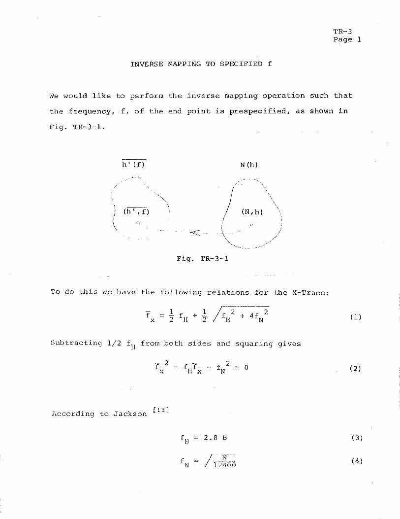
TR- 3 Page 1
INVERSE PING TO SPECIFIED f
W e would P i k e to pe r fo rm t h e i n v e r s e mapping o p e r a t i o n such t h a t
t h e f r e q u e n c y , f , o f t h e end p o i n t i s p r e s p e c i f i e d , a s shown i n
P i g . TR-3-1.
F ig . TR-3-1
To d o t h i s w e have t h e f o l l o w i n g r e l a t i o n s for t h e X-Trace:
S u b t r a c t i n g 1 / 2 fI1 from botlr s i d e s and s q u a r i n g g i v e s
According t o J a c k s o n l 1 3 1
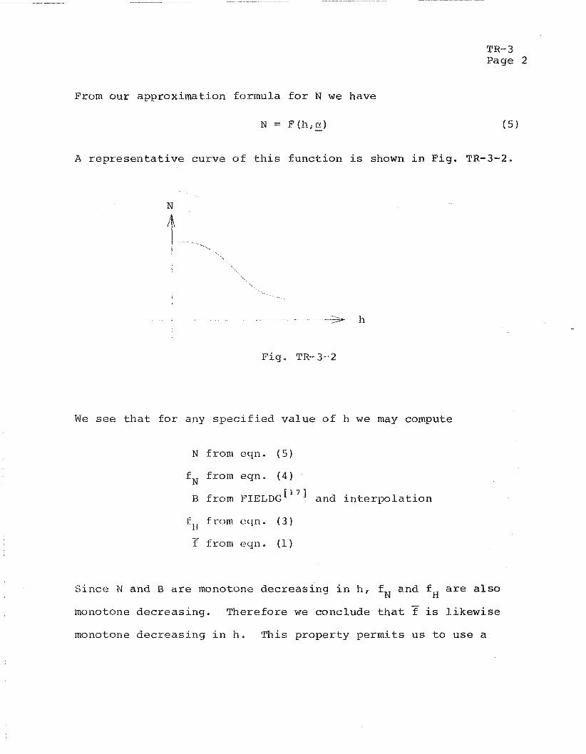
TR- 3 Page 2
From o u r approx imat ion formula f o r N w e have
N = F(lr,cxJ
A r e p r e s e n t a t i v e c u r v e o f t h i s f u n c t i o n i s shown i n F i g . TR-3-2.
Fig . TR-3-2
W e see t h a t f o r any s p e c i f i e d v a l u e o f h w e may compute
N from eqn. ( 5 )
f f rom eqn. ( 4 ) N
B from FIELDG and i n t e r p o l a t i o n
f r o m cyn . ( 3 ) - f from ecln. (1)
S i n c e N and B a r e monotone d e c r e a s i n g i n h , f and fH a r e also N
monotone d e c r e a s i n g . T h e r e f o r e w e conc lude t h a t 7 is l i k e w i s e
monotone d e c r e a s i n g i n h . T h i s p r o p e r t y p e r m i t s u s t o u s e a
TR- 3 Page 3
successive approximation technique for finding h 3 i f ; £ 1 -- A convenient algorithm for this purpose is Bolzanovs root finding
* technique.
We may elect to select h to within some given tolerance or to
iterate until 0 < - f < e . Figures TR-3-3, TR-3-4, and - I f I TR-3-5 show h selected to within -01% of a maximum value.
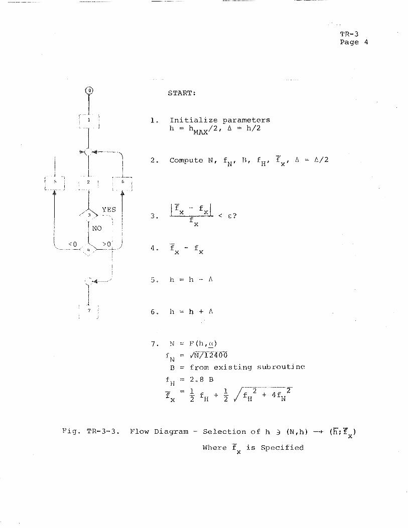
TR- 3 Page 4
START :
1, I n i t i a l i z e p a r a m e t e r s 11 = h / 2 , A = h / 2
MAX
- Compute N, fN, B f fII , fx, A = A/2
B = f rom e x i s t i n g s u b r o u t i n e
f,, = 2.8 B
- - F i g . T R - 3 - 3 . Flow Diagram - S e l e c t i o n of h 3 (Nth) + (h:fx)
Where 7 i s S p e c i f i e d X

TR- 3 Page 5
--
START:
Initialize parameters / 2 , A = h/2
- - Compute N, fN, f o - fN, A = A / 2
F i g . TR-3-4 . Flow Diagram - S e l e c t i o n o f h 3 ( N . h ) -+ (K:fo)
Where fo i s S p e c i f i e d
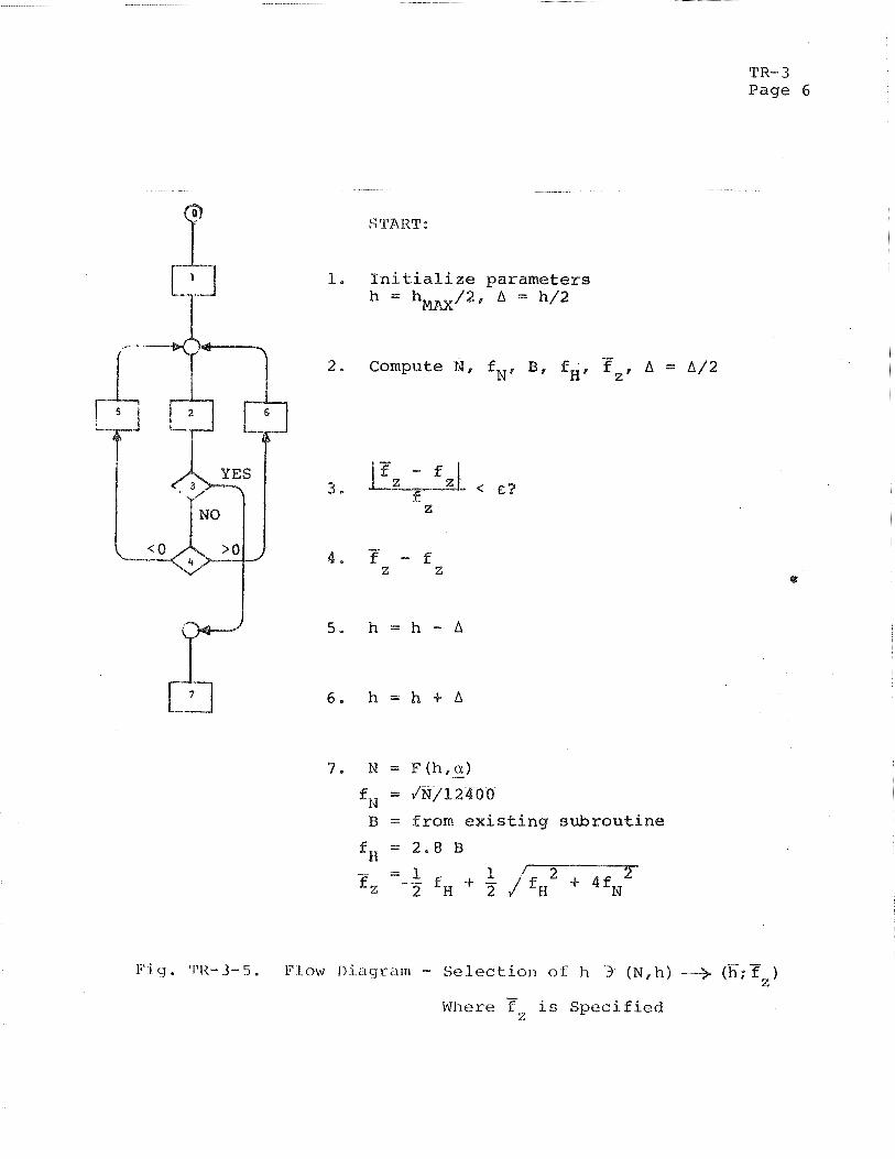
TR- 3 Page 6
Initialize parameters / 2 , A = h/2
Compute N. fN, B, fH,
7 . N = F ( h , g )
f, = JN/12400
B = from existing subroutine
f H = 2.8 B
I ' 1'1-3-5. F l o w D i a g r i l m - Selection of h 3 (N, h ) (f;;Y ) z
- Where f is Specified
I,
P r e p a r e d fo r :
A s t r o d a t a , Inc . 248 E , P a l a i s R d .
A n a h e i m , C a l i f ,
A s t r o d a t a P r o j e c t 9 38400
TI?- 4
SIpfPEIFICA'I ' ION OF MATRIX INVERSION PROBLEM
J o h n F. K i n k e l T e c h n i c a l C o n s u l t a n t Newport B e a c h , Calif.
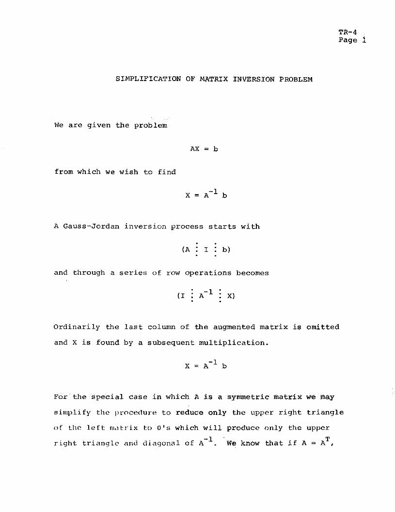
TR-4 .
Page i
SIMPLIFICATION OF MATRIX INVERSION PROBLEM
We are given t h e problem
AX = b
from which w e wish t o f i n d
X = A - l b
A Gauss-Jordan i n v e r s i o n process starts wi th
and through a series of r o w ope ra t ions becomes
Ord ina r i ly t h e l a s t column of t h e augmented ma t r ix is omi t ted
and X i s found by a subsequent m u l t i p l i c a t i o n .
X = A-’ b
a1 c i n A m
s i n i p l i f y the procedure t o reduce only t h e upper r i g h t t r i a n g l e
o f thc! l e f t , riiciti-ix to 0 ’ s which w i l l produce only t h e upper
r i g h t triangle arid d iagonal of A w l e ‘We know t h a t i f A = AT,
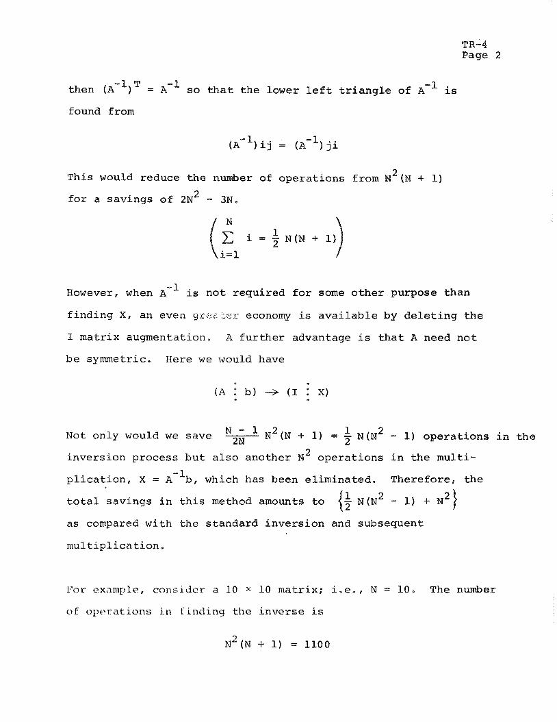
TR-4 Page 2
-1 T -1 then (A ) = A s o t h a t t h e lower l e f t t r i a n g l e of A-l is
found from
This would reduce t h e number of o p e r a t i o n s from N L ( N + 1)
f o r a s a v i n g s o f 2 N 2 - 3N.
However, when A-l is n o t r e q u i r e d f o r some o t h e r purpose than
f i n d i n g X , an even grcrz':e.r economy i s a v a i l a b l e by d e l e t i n g t h e
I m a t r i x augmentation, A f u r t h e r advantage is t h a t A need n o t
b e symmetric. H e r e we would have
Not on ly would we s a v e 2N 1 -
N 2 ( N + 1) = 7 N ( N ~ - 1) o p e r a t i o n s i n t h e
i n v e r s i o n p roces s b u t a l s o ano the r M2 o p e r a t i o n s i n t h e mu l t i -
-1 p l i c a t i o n , X = A b , which has been e l imina t ed . The re fo re , t h e
t o t a l s av ings i n t h i s method amounts t o N ( N 2 - 1) + N 2
a s compared w i t h t h e s t a n d a r d i n v e r s i o n and subsequent
m u l t i p l i c a t i o n ,
F o r example, cons1dc.r a 1 0 x 10 mat r ix ; i , e , , N = 10. The number
o f opera t ions i n f i n d i n g t h e i n v e r s e is

TR- 4 Page 3
The subsequent m u l t i p l i c a t i o n requ i res an a d d i t i o n a l N~ = 100
f o r a t o t a l of 1200 opera t ions ,
Finding X d i r e c t l y and n o t A-I r e q u i r e s N(N + 1 j 2 = 605 Z opera t ions for a savings of 595,
This agrees with t h e express ion f o r savings of ~ ( 8 ~ - 1) + N 2 C
1 - 990 + 100 = 595* Therefore, f o r N reasonably l a r g e , say N > 10, 2 - t h e savings amounts t o almost 50%,
Subroutine MXV for computing - x, where
i s l i s t e d on the fol lowing page,

Prepared for:
Astrodata, Inc, 24Q E , Palais Rd. Anaheim, Calif.
Astrodata Project 938400
TR- 5
TIME3 SKEW PROBLEM
December 12, 1 9 6 9
John F , Kinkel Technical Consultant N e w p o r t Beach, Calif,
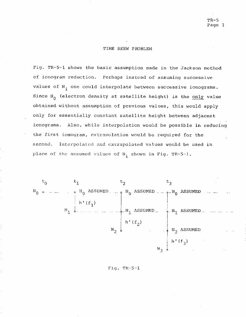
TR- 5 Page 1
TIME SKEW PROBLEM
F i g - TR-5-1 shows t h e b a s i c assumption made i n t h e Jackson method
of ionograni r e d u c t i o n , Perhaps i n s t e a d of assuming succes s ive
va lues of N i one could i n t e r p o l a t e between s u c c e s s i v e ionograms.
S ince No ( e l e c t r o n d e n s i t y a t s a t e l l i t e h e i g h t ) is t h e va lue
ob ta ined w i t h o u t assumption of p rev ious v a l u e s , t h i s would apply
on ly f o r e s s e n t i a l l y c o n s t a n t s a t e l l i t e h e i g h t between a d j a c e n t
ionograms. Also, whi le i n t e r p o l a t i o n would be p o s s i b l e i n reduc ing
t h e f i r s t ionogram, e x t r a p o l a t i o n would be r e q u i r e d f o r t h e
second, I n t e r p o l a t e d and extrapolated va lues would be used i n
p1;tce of t h e assumcd va lues of N shown i n F ig . TR-5-1. i
?! ASSUMED - - - No ASSUMED .-No ASSUMED S
I I I I i
-- ,& NI ASSUMED. -
1
P i g . TR-5-1
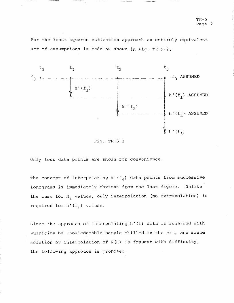
TR- 5 Page 2
For t h e l e a s t s q u a r e s e s t i m a t i o n approach an e n t i r e l y e q u i v a l e n t
s e t o f assumpt ions i s made a s shown i n F i g , TR-5-2,
. -- - f o ASSUMED £0 I - ? -
-- I - P h ' ( f l ) ASSUMED
h ' (5) I I
h ' ( f 2 ) ASSUMED -
I
Only f o u r d a t a p o i n t s are shown f o r convenience .
The c o n c e p t o f i n t e r p o l a t i n g h ' ( f i ) d a t a p o i n t s from s u c c e s s i v e
ionograms i s immedia te ly obvious from t h e l a s t f i g u r e . Unl ike
t h e c a s e f o r Ni v a l u e s , o n l y i n t e r p o l a t i o n (no e x t r a p o l a t i o n ) is
r e q u i r e d f o r h ' ( f i ) v a l u e s .
: t l l r l 1 ~ ' f i n 1 a t r 1 ' ( f ) c l a l . . ~ i s regarded wi t h
s u s p i c i o n by knowledqcable peop le s k i l l e d i n t h e a r t , and s i n c e
s o l u t i o n by i n t e r p o l a t i o n o f N (11) i s f r a u g h t w i t h d i f f i c u l t y .
t h e f o l l o w i n g approach i s p roposed ,
TR- 5 Page 3
1. I n t e r p o l a t e h g ( f ) a s desc r ibed above,
2 , Compute N (h ) from i n t e r p o l a t e d ?.I' ( f ) d a t a .
3 , I n t e r p o l a t e 14 ( h ) as ob ta ined i n s t e p 2 i n order t o
compute h ' ( f ) .
4 . If h l ( f ) agrees w i th h s ( f ) , t hen w e have found N ( h )
p r o f i l e s which when i n t e r p o l a t e d y i e l d r e s u l t s
matching t h e p h y s i c a l measurements,
P r e p a r e d for:
A s t rodata , Inc . 240 E , P a P a i s Rd.
A n a h e i m , C a l i f .
A s t r o d a t a P r o j e c t 938400
TR- 6
BPTIfiIAL STEP S I Z E BY ONE DIMENSIONAL SEARCH
D e c e m b e r 30, 1 9 6 9
John I?'. K i n k e l T e c i ~ n i c a l Coilsul tant N c w p o r t Beach, C a l i f .
TR-6 Page 1
OPTIPrylL STEP SIZE
BY ONE DIMENSIONAL SEARCH
The computa t ion of s t e p s i z e u s i n g t h e Hess ian m a t r i x i s b a s e d
on t h c assumpt ion t h a t t h e c o s t f u n c t i o n a l can bc r e a s o n a b l y
w e l l approximated by a t r u n c a t e d T a y l o r series h a v i n g t e r m s o f
no h i g h e r o r d e r than second . T h i s assumpt ion i s f r e q u e n t l y
u n j u s t i f i e d r e s u l t i n g i n a s t e p s i z e which may b e e i t h e r t o o
l a r g e o r t o o s m a l l , "%>r +he c a s e i n which t h e s t e p s i z e is t o o
s m a l l t h e c o s t r e d u c t i o n a t e a c h i t e r a t i o n i s less t h a n c o u l d
b e a c h i e v e d r e s u l t i n g i n t h e need f o r more i t e r a t i o n s t h a n
n e c e s s a r y f o r convergence . A more s e r i o u s d e f e c t o c c u r s f o r t h e
c a s e i n which t h e s t e p s i z e i s t o o l a r g e ; i n t h i s case t h e cost
may i n c r e a s e f o r some i t e r a t i o n s , s e r i o u s l y i m p a i r i n g , i f n o t
complc tc ly p r e v e n t i n g , convergence t o t h e o p t i m a l s o l u t i o n .
T h i s e f f e c t has bcen n o t e d i n p r a c t i c e .
S i n c c w e know t h a t t h e r e e x i s t s sonle s t e p s i zc .in t h e g r a d i e n t
d i r e c t i o n which i f s u f f i c i e n t l y s m a l l w i l l p roduce a d e c r e a s e i n
c o s t , w e s h o u l d be a b l e t o produce a c o s t r e d u c t i o n i n e v e r y
i t e r a t i o n u n t i l t h e o p t i m a l s o l u t i o n is ach ieved . What w e would
l i k e t o do i s t o f i n d t h e s t e p s i z e t h a t w i l l y i e l d t h e g r e a t e s t
r e d u c t i o n i n cost f o r each i t e r a t i o n . T h i s o p t i m a l s t e p s i z e
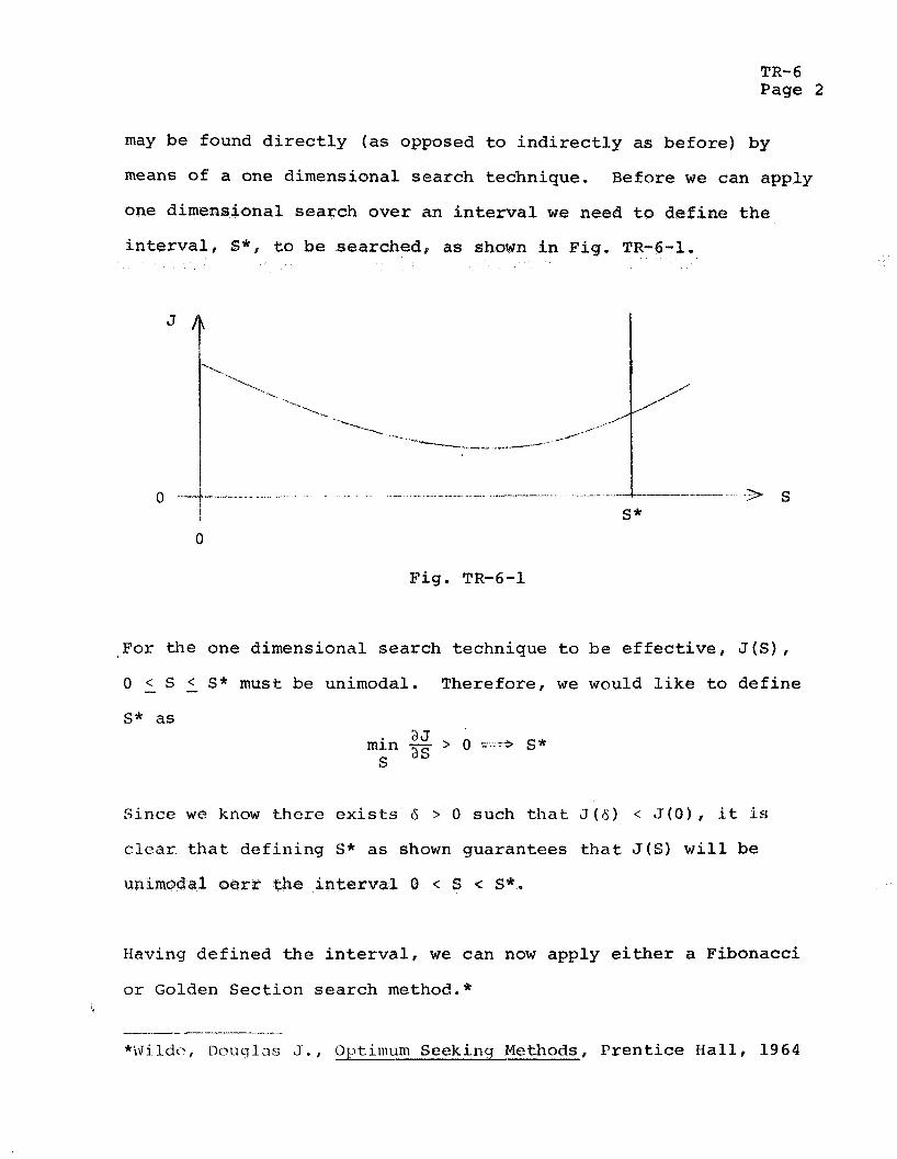
TR-6 Page 2
may be found d i r e c t l y (as opposed t o i n d i r e c t l y as be fo re ) by
means of a one dimensional s ea rch technique. Before w e can apply
one d i ch ove r an i n rval w e need t o
i n t e r v a l , S * , t o be searched , a s shown i n Fig. *
/ /
i 0
Fig . TR-6-1
S"
For t h e one dimensional search technique t o b e e f f e c t i v e ,
0 - < S - < S* must be unimodal. Therefore , w e would l i k e t o
t h e
-3 s
J (S ) ?
d e f i n e
S* a5
Sincc w e know there e x i s t s 6 > 0 such t h a t J(((;) < J ( O ) , it i s
clear, t h a t d e f i n i n g S* a s shown guarantees t h a t J ( S ) w i l l be
Having de f ined t h e i n t e r v a l , we can now apply e i t h e r a Fibonacci
or Golden Sec t ion sea rch method.*
*Wild<>, nnuqlas J, , O j t i r n u m Seeking Methods, P r e n t i c e Ha l l , 1 9 6 4
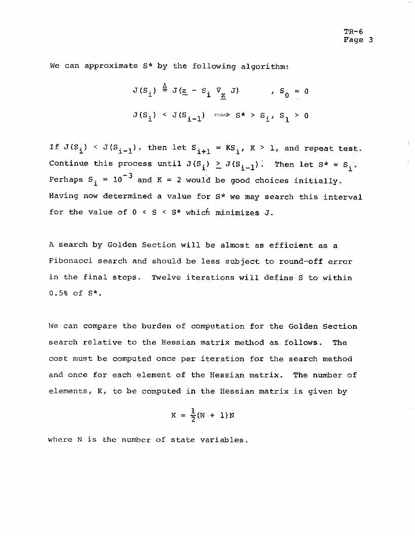
TR- 6 Page 3
W e can approximate S* by t h e fo l lowing a lgor i thm:
J ( S i ) 4 J(z - Si Vz J) S o = O -
J ( S i ) < J(Siml) ~ ' 3 S* > S i~ s1 > 0
If J f S i ) < J(Si- l ) . t hen l e t Si+l = KSiP K 1, and r e p e a t test .
Continue t h i s p rocess u n t i l J ( S i ) - > J ( S i - 1) : Then l e t S* = Si. - 3 Perhaps Si = 10 and K = 2 would b e good cho ices i n i t i a l l y .
Having now determined a va lue f o r S* w e may s e a r c h t h i s i n t e r v a l
f o r t h e v a l u e of 0 < S < S* which minimizes J.
A s e a r c h by Golden S e c t i o n w i l l be a lmost as e f f i c i e n t as a
F ibonacc i s e a r c h and shou ld be l e s s s u b j e c t t o round-off e r r o r
i n t h e f i n a l s t e p s . Twelve i t e r a t i o n s w i l l d e f i n e S t o w i t h i n
0,5% of S*.
W e can conipare t h e burden of computation f o r t h e Golden S e c t i o n
s e a r c h r e l a t i v e t o t h e Hessian m a t r i x method a s fo l lows . The
c o s t must b e computed once p e r i t e r a t i o n f o r t h e s e a r c h method
and once f o r each e lement of t h e Hessian m a t r i x , The number o f
e lements , K , t o b e computed i n t h e Hessian m a t r i x i s g iven by
where N i s the number of s t a t @ v a r i a b l e s .
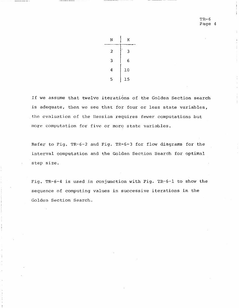
TR- 6 Page 4
I f w e assume t h a t twelve i t e r a t i o n s of t h e Golden S e c t i o n sea rch
i s adequa te , then w e see t h a t f o r f o u r o r l e s s s t a t e v a r i a b l e s ,
the e v a l u a t i o n of the Hessian r e q u i r e s fewer computations but
more computation fo r f i v e o r more s t a t e v a r i a b l e s .
Refer t o F ig . TR-6-2 and Fig . TR-6-3 f o r flow diagrams f o r t h e
i n t e r v a l computation and t h e Golden Sec t ion Search f o r op t imal
. s t e p s i z e .
F ig . TR-6-4 is used i n conjunc t ion wi th F ig . TR-6-1 t o show t h e
sequence of computing va lues i n s u c c e s s i v e i t e r a t i o n s i n t h e
Golden Sec t ion Search.
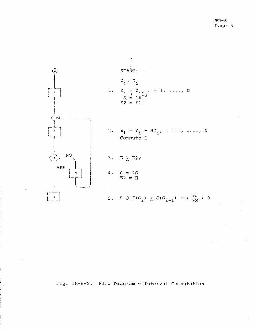
TR- 6 Page 5
2. Zi = Yi - S D i , i = 1, . . . . , N Compute E
P i g , TR-6-2 , Flow Diagram - Interval Computation
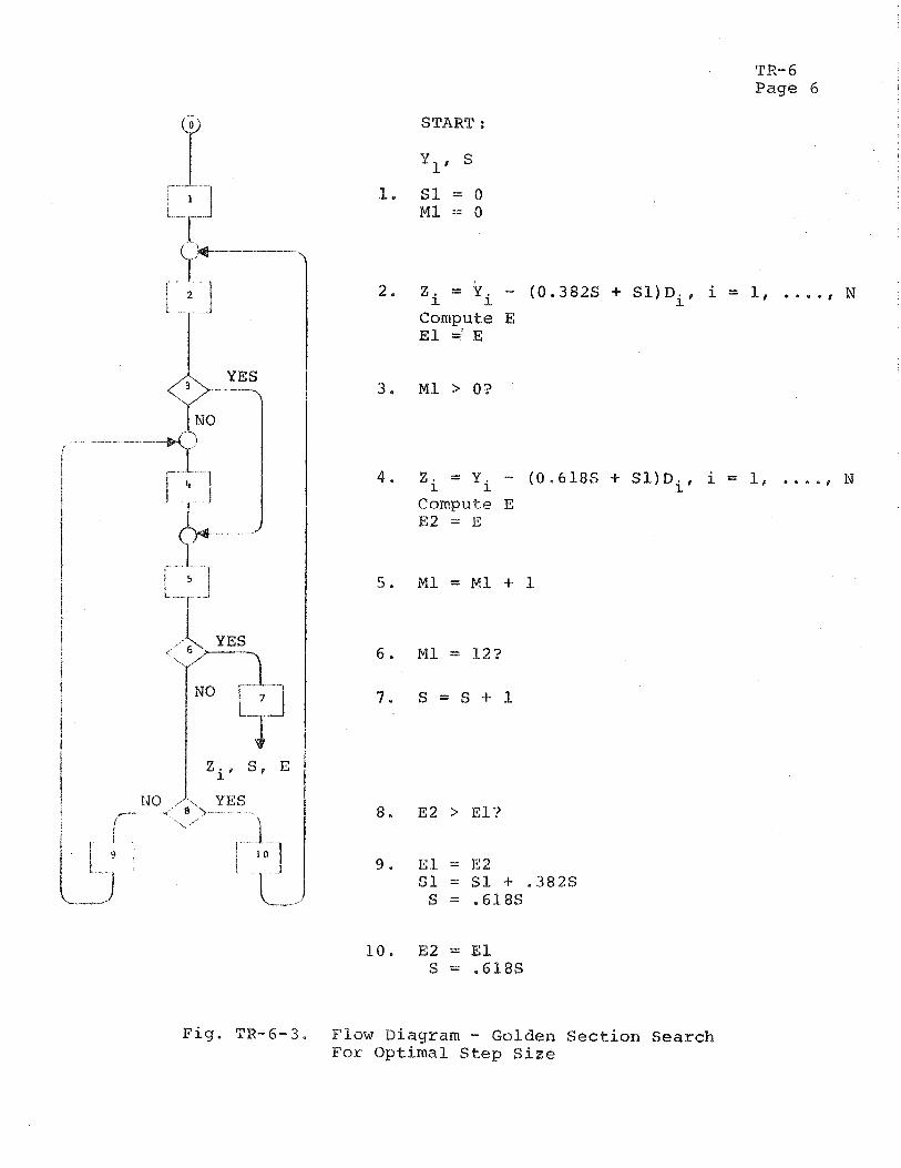
TI?-6 Page 6
START :
Y1, S
I* S Z - 0 M1 -= 0
Compute E El =' E
- 4. Z i - Yi - ( 0 . 6 1 8 5 + S1)Di, i = 1 # ...., N Compute E E 2 = E
8, E 2 > E l ?
Fig. TR-6-3. Flow Diagram - Golden Sec t ion Search For Optimal Step Size
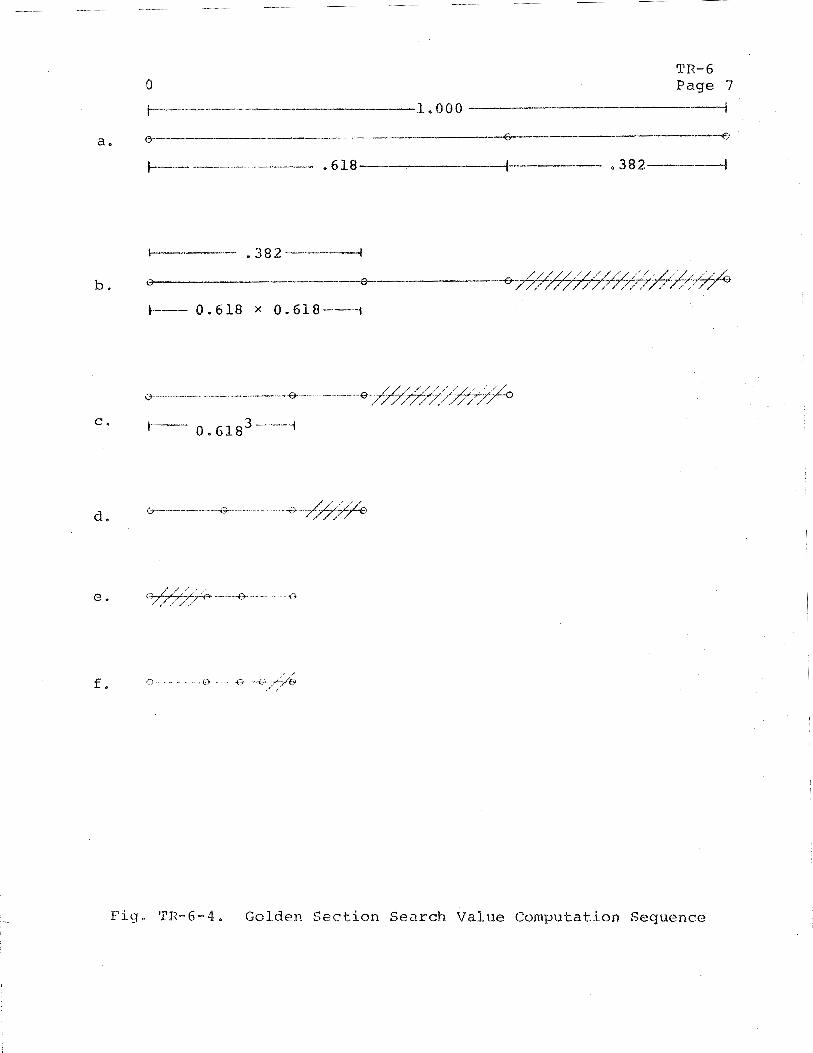
TR-6 0 Page 7
.-*-------.------ 1 * 0 0 0 ---------
r i g . TR-6-4. Go lden S e c t i o n Search V a l u e Computat.ion Secluence
P r e p a r e d for:
A s t rodaka, Inc , 240 Ee Palais Rd,
A n a h e i m , C a l i f ,
Astrodata P r o j e c t 938400
TR- 7
HORIZONTAL PROCESSING
J a n u a r y 3 0 , 1970
John F. K i n k e l T c e h n i c a l Consultant Newport B e a c h , C a l i f .
TR- 7 Page 1
HORIZONTAII PROCESSING
I n t r o d u c t i o n
Because of t h e motion o f t h e satsLlite r e l a t i v e t o the e a r t h , it
is a b a s i c p r o p e r t y of t h e swept f requency technique t h a t w i t h i n
t h e same ionogram s u c c e s s i v e h D (f) d a t a poir i t s correspond t o
soundings taken through t h e ionosphere a t d i f f e r e n t e a r t h based
coo rd ina t e s (see Fig, TR-7-1).
I t is i m p l i c i t l y assumed i n c u r r e n t l y a p p l i e d d a t a p roces s ing
methods f o r conve r t i ng h Y f ) d a t a t o N(h) p r o f i l e s t h a t t h e
e l e c t r o n d e n s i t y p r o f i l e i s c o n s t a n t over t h e s e c t i o n o f ionosphere
t r a v e r s e d by t h e s a t e l l i t e du r ing t h e pe r iod o f one ionogram.
This assumption is r e q u i r e d n o t on ly f o r t h e l amina t ion technique
of Jackson [' ( f o rna rd p roces s ing ) and Madsen* ( i n v e r s e p roces s ing )
b u t a l s o f o r t h e l e a s t squa re s e s t i m a t i o n technique desc r ibed
e lsewhere i n t h i s r e p o r t . The e r r o r i n t h e e l e c t r o n d e n s i t y
p r o f i l e r e s u l t i n g from t h i s assumption is n o t known.
I lor izontal processing is a method of d a t a r e d u c t i o n which does
not r e q u i r e t h e assumption of c o n s t a n t N(h) p r o f i l e over t h e
s e c t i o n r e q u i r e d by one ionogram, I n h o r i z o n t a l p roces s ing
e l e c t r o n d e n s i t y va lues a long t h e s a t e l l i t e t r a c k are e s t ima ted
*See S e c t i o n 111, t h i s r e p o r t
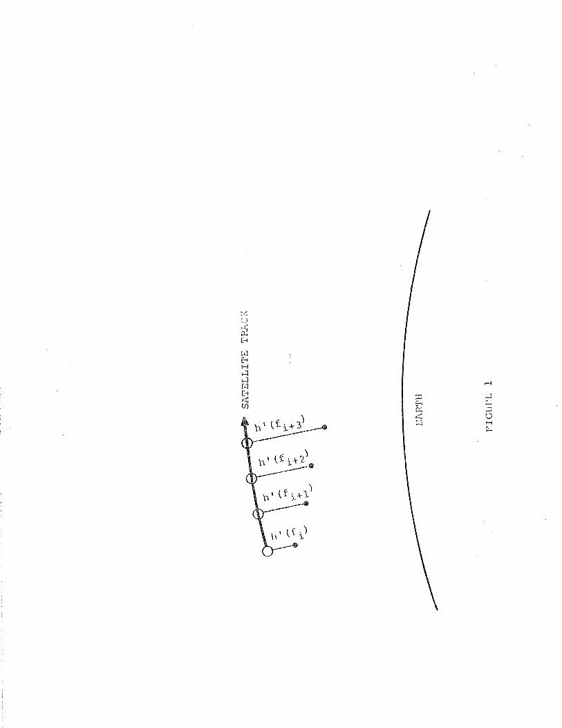
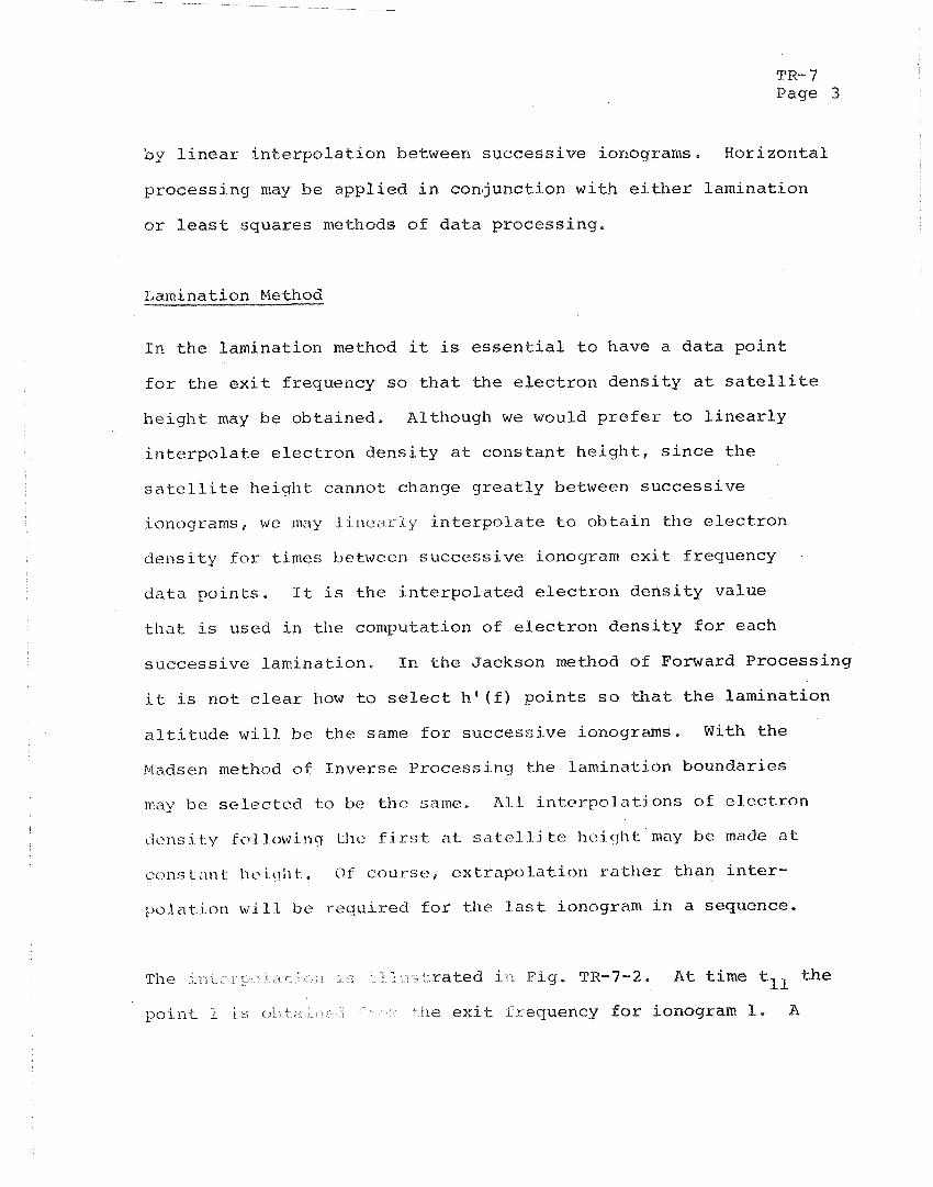
TR- 7 Page 3
by l i n e a r i n t e r p o l a t i o n between s u c c e s s i v e ionograms. H o r i z o n t a l
p r o c e s s i n g may b e a p p l i e d i n c o n j u n c t i o n w i t h e i t h e r l a m i n a t i o n
o r l e a s t s q u a r e s methods o f d a t a p r o c e s s i n g .
Laminat ion Method
I n t h e l a m i n a t i o n method it is e s s e n t i a l t o have a d a t a p o i n t
for t h e e x i t f r equency so t h a t t h e e l e c t r o n d e n s i t y a t s a t e l l i t e
h e i g h t may b e o b t a i n e d , Although w e would p r e f e r t o l i n e a r l y
i n t e r p o l a t e e l e c t r o n d e n s i t y a t c o n s t a n t h e i g h t , s i n c e t h e
s a t e l l i t e h e i g h t canno t change g r e a t l y between s u c c e s s i v e
ionograms, w e may linedrly i n t e r p o l a t e t o o b t a i n t h e e l e c t r o n
d e n s i t y f o r times bctweeii s u c c e s s i v e ionogram e x i t f r equency
d a t a p o i n t s . I t is t h e i n t e r p o l a t e d e l e c t r o n d e n s i t y v a l u e
t h a t is used i n t h e computa t ion o f e l e c t r o n d e n s i t y f o r each
s u c c e s s i v e l a m i n a t i o n . I n t h e Jackson method o f Forward P r o c e s s i n g
i t i s n o t c l e a r how t o select h f ( f ) p o i n t s s o t h a t t h e l a m i n a t i o n
a l t i t u d e w i l l be t h e same f o r s u c c e s s i v e ionograms. With t h e
Madsen method of I n v e r s e P r o c e s s i n g t h e l a m i n a t i o n b o u n d a r i e s
may bc s e l e c t e d t o bc t h e same. A l l i n t c r p o l a t j o n s o f e l e c t r o n
t - ic .nr ; i t)' fnllc%\ri nq tht: f i r s t at s a t c l l j tc h c i ( ~ h t may be made a t
con:: t a n t ficityh t . O f COUI-SO cxt rapo l a t i n n riltlier t h a n i n t e r -
p o l a t i o n will b e r c q u i r e d f o r t h e l a s t ionogram i n a sequence ,
r a t e d is> Fig. TR-7-2. A t t i m e tll t h e
'le e x i t f r equency f o r ionograrr? 1, A
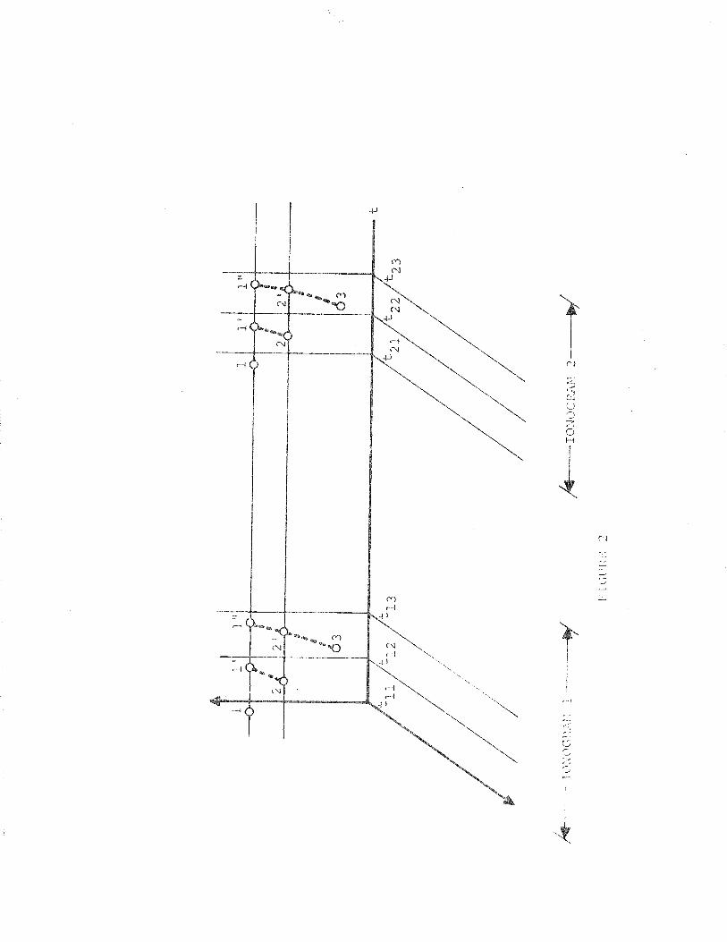
TR- 7 Page 5
s imi l a r p o i n t is ob ta ined f o r t i m e t21 from ionogram 2 .
d a t a p o i n t i s selected corresponding t o a t i m e t12.
now e x t r a p o l a t e d forward i n t i m e t o tL2, g i v i n g p o i n t 1 @ a The
e l e c t r o n s i t y a t p o i n t 1' i s used t o compute p o i n t 2. This
process is cont inued u n t i l t h e l as t u s e f u l data p o i n t has been
processed, say p o i n t j . Then w e w i l l have a complete N(h) p r o f i l e
corresponding t o t i m e t f o r t h e f i rs t ionogram, t for t h e
second, etc.
An h ' ( f )
P o i n t 1 i s
I
l j 2 j
I n the l amina t ion method t h e r e are t w o p o s s i b l e approaches f o r
t h e i n t e r p o l a t i o n of e l e c t r o n d e n s i t y a t s a t e l l i t e h e i g h t .
T h e f i r s t o f these is j u s t t o f i n d
whcre
N . ( f i , t ) = e l e c t r o n d e n s i t y a t h e i g h t h and t i m e t 1
from jth ionogram
JT h e i g h t from Ith p o i n t from jth ionagrrrm hi j tij = t i m e of ith p o i n t from jth ionogram
TR- 7 Page 6
The second approach i s t o f i n d t h e e l e c t r o n d e n s i t y from t h e
ionogram having t h e h i g h e r sa te l l i te p o s i t i o n a t t h e s a t e l l i t e
h e i g h t o f t h e a d j a c e n t ionogram wi thou t i n t e r p o l a t i o n , This
s t e p i s e a s i l y j u s t i f i e d because o f t h e very sma l l t i m e i n t e r v a l
involved i n Lhis c a s e , To b e s p e c i f i c , suppose t h a t
hl, j + l h l j
f\Towr us ing t h e lladsen I n v e r s e P roces s ing technique , w e can f i n 6
where w e have selected h L , - , j+ l - h l j e
Using t h i s va lue of N j + l
w e can i n t e r p o l a t e PJ a t constant . h e i g h t a s j
For e i t h e r o f t h e s e c a s e s succeeding i n t e r p o l a t i o n s may be made
a t c o n s t a n t h e i g h t a s fol lows:
By t h i s means we may compute s u c c e s s i v e l amina t ions a s shown by
F i g . TR-7-3 .
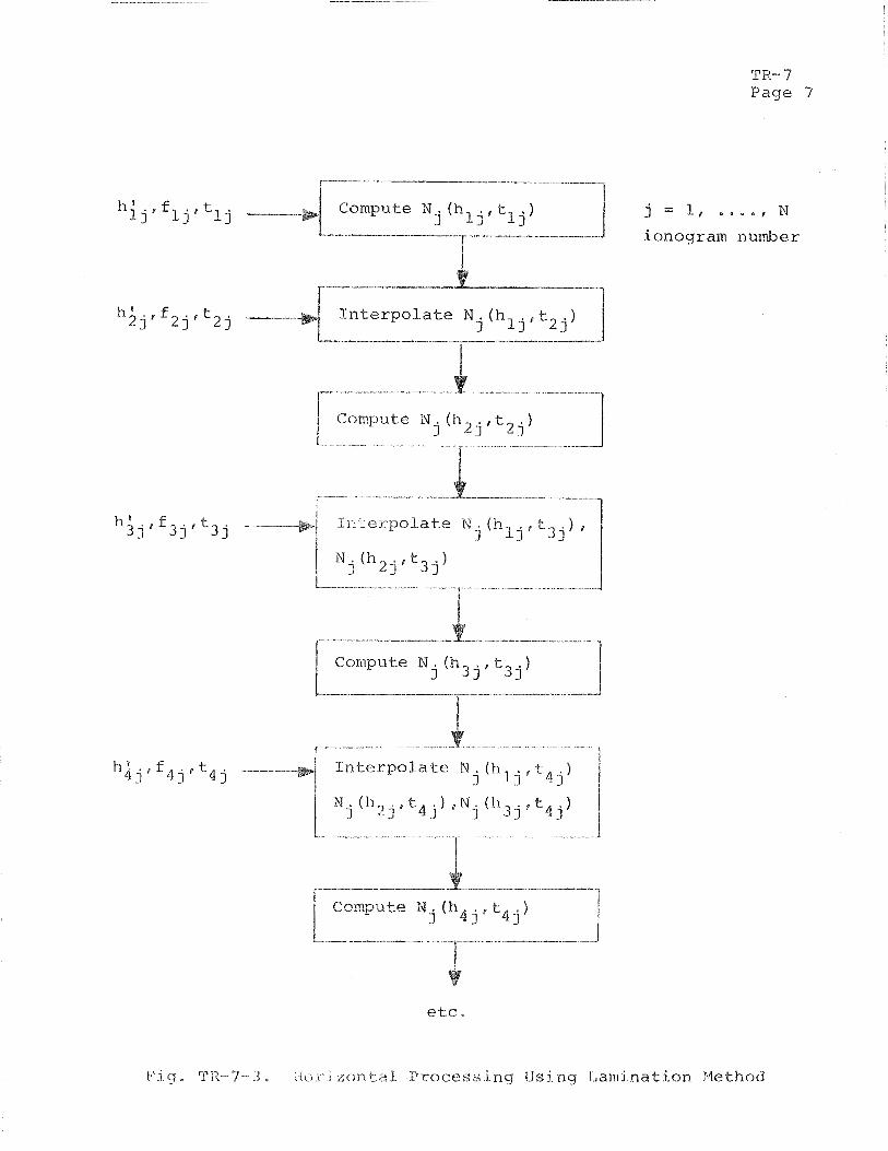
TR- 7 Page 7
-
f j j Compute N . (hl j. tl j) J
j = l t . * w e , N
ionogram number
I n t e r p o l a t e N . (hl j. t2 J
-
Compute N ( h j tj j) 3
Compute N (h4j,t ) j 4 j
v e t c
i g 3 tior i zor-at,%l Processing Using Laminat ion PTethod
TR-7 Page 8
D i f f i c u l t y w i l l b e e n c o u n t e r e d , of c o u r s e , w i t h ionogram sequences
i n which few s u c c e s s i v e comple te ionograms a r e a v a i l a b l e . En
t h e s e c a s e s i n t e r p o l a t i o n i n c o n j u n c t i o n w i t h a l e a s t s q u a r e s
e s t i m a t i o n may o f f e r a s o l u t i o n ,
L e a s t S a u a r e s E s t i m a t i o n
P a r t h i s method t h e i n i t i a l e s t i m a t e f o r N(h) is de te rmined
wi thout . e x t r a p o l a t i o n . S u c c e s s i v e r e v i s i o n s to t h i s e s t i m a t e u s i n g
i n t e r p o l a t i o n a r e t h e n de te rmined i t e r a t i v e l y i n o r d e r t o improve
t h e e s t i m a t e . A s shown i n F i g . TR-7-4, t h e i n i t i a l t ime skewed N ( h )
p r o f i l e s arc c ics t c l rn l l lleci w r t i ~ o u t r e g a r d t o chanqe i n N ( h ) p r o f i l e s
w i t h p o s i t i o n alor~q the t r a c k . Using c o n s t a n t h ( o r n e a r l y s o )
i n t e r p o l a t i o n , a sequence o f N(h) p r o f i l e s c o r r e s p o n d i n g t o
c o n s t a n t t i m e a r e found, T h i s sequence of c o n s t a n t t i m e N(h)
p r o f i l e s i s used i n t h e i n v e r s e mapping p r o c e s s i n t h e second
i t e r a t i o n t o f i n d an improved e s t i m a t e o f t h e t i m e skewed N ( h )
p r o f i l e . A l l ionograms i n a sequence a r e p r o c e s s e d i n t h i s
manner b e f o r e p roceed ing t o t h e n e x t i t e r a t i o n , T h i s p r o c e s s o f
c s t - ima t inq t i m c s k e w e c l p r o f i l c s fo l lowcd by j n t e r p n l a t i o n may be
t . ' c -~- I o1-mclci :;c.c~uci~t i ,I l l y t (> i mprc)vc. t l l c l e:; k i r n d t c x , A s '3 l i n a l stc?p
t l l ( % I I ~ ; l i ~ ~ ~ c ~ < l N (11 ) 111-0 r i 1 cxs , t r - c b i rl L c . r ] ) o l n t c b t l to t tic. clc.:; i r c > d
c.orl:; t , ~ n t t i n ~ c N (11) pro f i l e .
W e know t h a t i n a c t u a l i t y t h e e l e c t r o n d e n s i t y p r o f i l e i s a
z'u:--t;-7< c;f poqi t i o n a9onct t h e s a t e l l i t e trace s o t h a t w e may
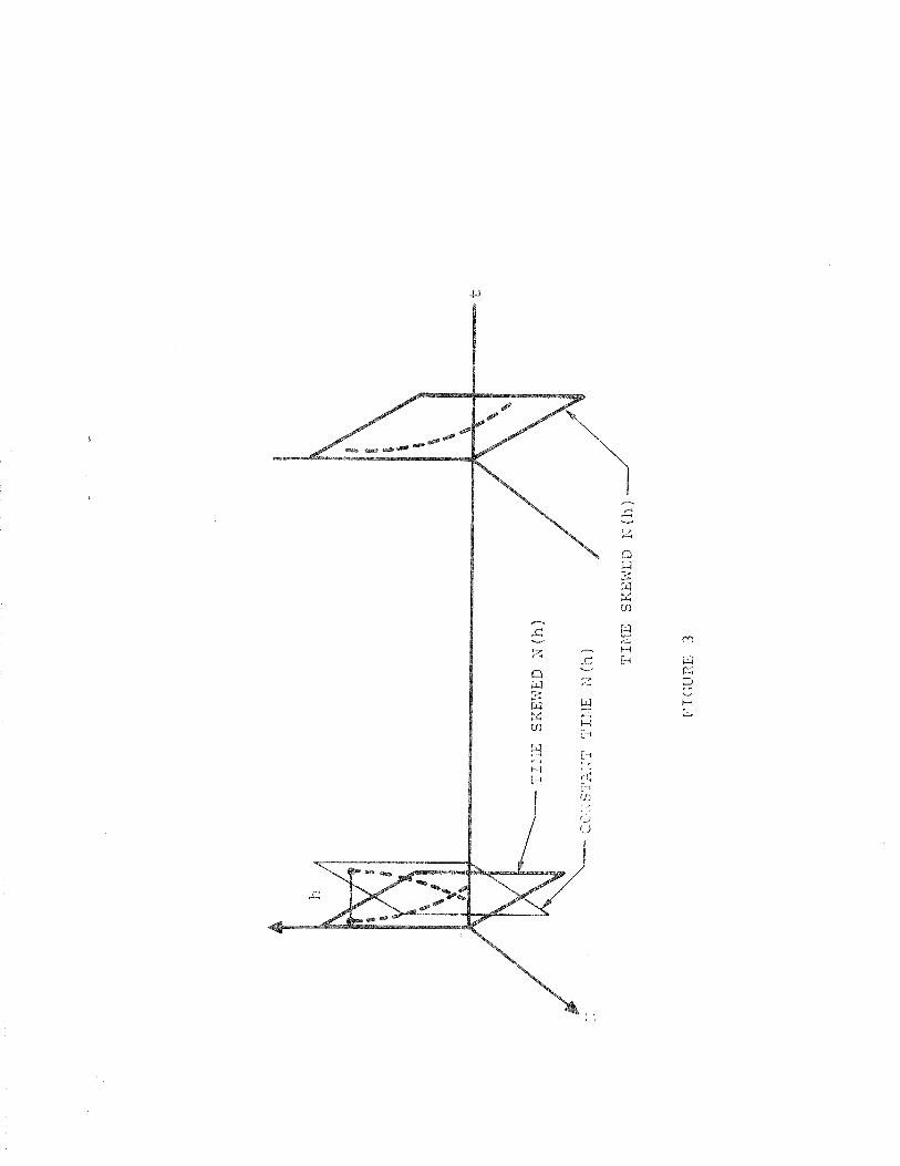
TR- 7 Paye 113
w r i t e t h e e l e c t r o n d e n s i t y approx imat ion
t)
For t h e l e a s t s q u a r e s method w e need t o use t h e i n v e r s e mapping
N i ( h i r g f t j I f i = 1, e . - - t j f ) j = 9, - . - * , J J J
where J =L number o f h g ( f ) d a t a p o i n t s .
Since t and f a r c uniquely r e l a t e d w i t h i n t h e t ime p e r i o d of one
ionogra~n w e may w r i t e t h a t
For t h e f i r s t i t e r a t i o n we mere ly u s e
However, f o r s & s e q u e n t i t e r a t i o n s w e f i n d
Ni tjI p r o j e c t e d on c o n s t a n t t i m e p l a n e
L 1 1 r)cx,1 t i 11t cl-t,o l < ~ i i c t l t '1:; clc.:;c-1 i l ) c ~ t f i n t l t c . p r - c . c c . ( l i ! - i c ~ :ictc:t i o n ,
T l ~ c ~ ~ - t ~ ! r ) t - c ~ a l l :;ul,sec]~-tc~~lt i t e r a t i o n s makc u s e of
For t h e l e a s t squares method t h i s p r o c e s s i s shown i n t h e f l o w
diagr ,
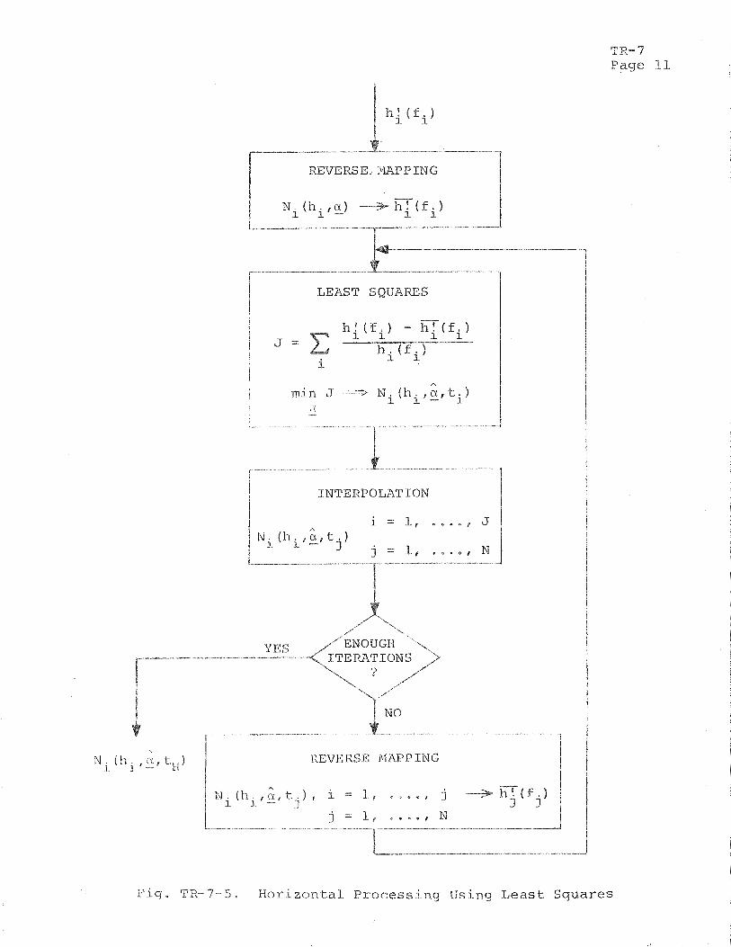
TR- 7 Page II
REVERS E , I U P P IN G
1 LEAST S Q U A E S t I
- - . --- -- -
INTERPOLATION
f
i t
N . ( h i , A , REVERSE MAPPING I
Fig, TR-7-5. Horizontal Processing Using Least Squares
Prepared fo r :
As trodata, Inc, 240 E , Palais Rd. Anaheim, Calif.
Astrodata Project 938400
TR- 8
C'OMl>LJ'L'/ 1 ' I ON O F TI I K l'S EUIIO THVl,: 1J.S 1;;
John F , Kinkel Technical Consultant
I ort Beac i~ , Calif,
TR- 8 Page l
Abstract
A new computational algorithm is proposed for constructing the
pseudoinverse of a matrix, The method is believed to be more
efficicnt for rnachinc computation than previous methods.

TR- 8 Page 2
I n t r o d u c t i o n
A problem which a r i s e s f r e q u e n t l y i n t h e a p p l i c a t i o n o f e s t i m a t i o n
t h e o r y ( ' I i s t o f i n d a b e s t e s t i m a t e o f - x from
where
I f A i s a s q u a r e m a t r i x of r a n k n t h e n - x i s u n i q u e l y d e t e r m i n e d f r o m
IIowcver, most f r e q u e n t l y A i s a r e c t a n g u l a r m a t r i x w i t h m :> n .
F o r t h e c a s e i n w h i c h t h e r ank o f A i s n , t h e l e a s t s q u a r e s estimate
c a n b e found from ( 2 )
> ~ ( A ~ A ) = n T
s i n c e r ( A ) = n > ( A A) i s n o n s i n g u l a r
( r ( A ) = r a n k o f A ) ,
T l l c ~ w c v c x - , f o r cases i i i w h i c l l r ( A f i n it f o l l o w s t h a t r ( A A ) 8 n
'P , - i l l l ! ( ) ; :; j 1 , - - I I c c ( 3 ) tloc.:; n o t a p p l y , I1'or L l l c 3 s c

TR-8 Page 3
cases the pseudoinverse ( 1 - 4 ) may be used, The pseudoinverse is
( 4 1 * defined by the following three requirements a
T .L T where y t- N ( A ) 2 E N (A ) T
- 2 M Z - = = O ( 7 )
N ( A l l is t i l l si~bspnce in E which is the orthogonal n
complement of l i l c t null space of A,
T I? (A ) is the restricted range space of AT in En,
R ( A ) I is the subspace in Em which is the orthogonal
complement of the restricted range of A,
N (iIT) is the null space of AT in Em.
'I'l~c.ri.fore, we call clc~compose E and E as fo l 1-ows : m I1
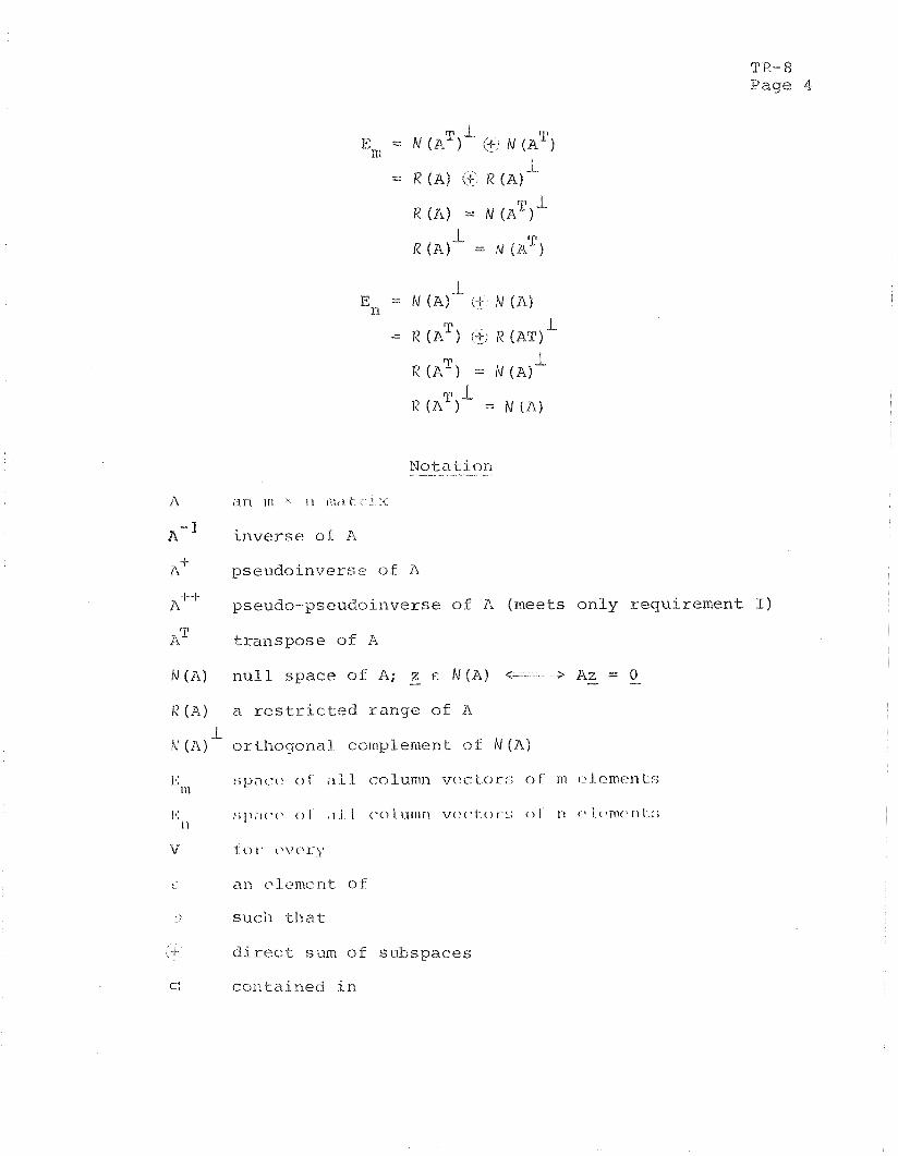
TR- 8 Page 4
T 1 R (A) = N (A )
_L E n = /d (A) t + M (A)
T = R (A ) i-k, R (AT)
L
A '311 It1 ' 11 Plat 1 :.:
A -1 inverse of PL
+ A pseudoinverse of A
A+' pseudo-pseudoinverse of A (meets only requirement I)
A* transpose of A
M(A) null space of A; - z E N ( A ) c- > Az - =
R(A) a restricted range of A
I N (A) orthogonal complement of I\d (A)
L:lll space of ; i l l column vc'et ctr:; o f m c.1 crnnnt:;
1'; ; , f , t I I ( - 0 1 urnri vc.cvt c , ~ - : ; 0 1 1 1 I ( * r ~ ~ c > r ~ t , : ; I I
> 4- direct sum of sdspaces
c: contained in
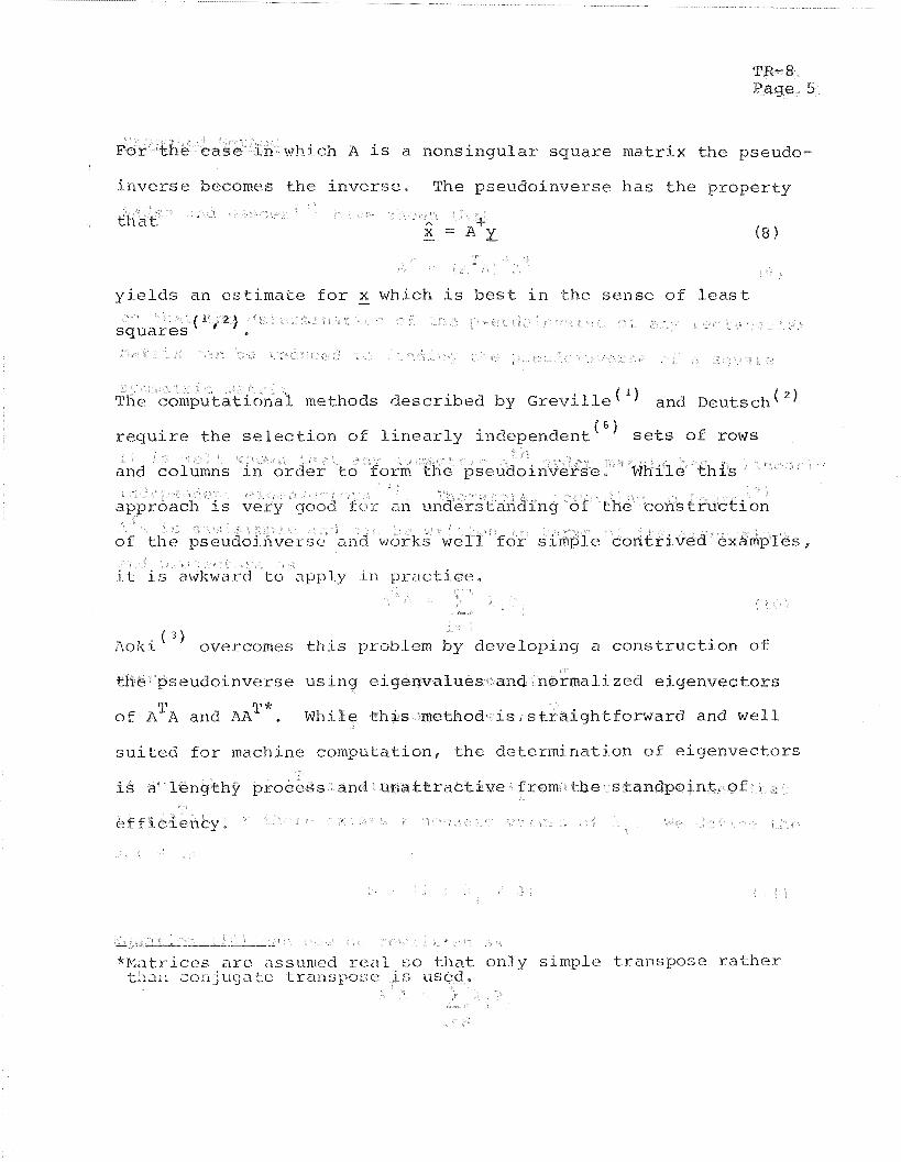
TR-8 Page 5
ich A is a nonsingular square matrix the pseudo-
inverse becomes the inverse, The pseudoinverse has the property
methods described by ~reville' and Deutsch ( 2 )
iiolt i ( 3 ) overcomes this problem by developing a construction of
the pseudoinverse using eigenvaLues and normalized eigenvectors
T of A X and MiT*- While this meth traightforward and well
suited for machine computation, the determination of eigenvectors
and unattractive from the standpoint of
y simple transpose rather
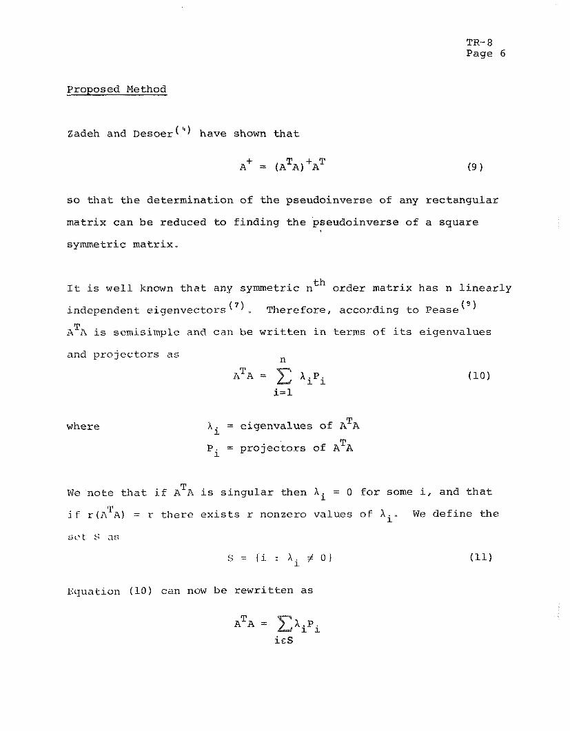
TR- 8 Page 6
Proposed Method
Zadeh and Desoer ( 4, have shown t h a t
T + T A+ = ( A A) A
s o t h a t t h e de t e rmina t ion of t h e pseudoinverse of any r e c t a n g u l a r
ma t r ix can be reduced t o f i n d i n g the pseudoinverse of a squa re
symmetric m a t r i x ,
I t is w e l l known t h a t any symmetric nth o r d e r ma t r ix has n l i n e a r l y
independent e i g e n v e c t o r s ( 7 ) . Therefore , accord ing t o Pease ( 9
T A A is semisimple and can be w r i t t e n i n t e r m s of i ts e igenva lues
and p r o j e c t o r s a s n
where T A i = e igenva lues of A A
T Pi = p r o j e c t o r s of A A
T W e n o t e t h a t i f A A i s s i n g u l a r t hen h i = 0 f o r some i, and t h a t
T i f r ( A A ) = r t h e r e e x i s t s r nonzero va lues of i" W e d e f i n e t h e
Eyunt , ion ( 1 0 ) can now be r e w r i t t e n as
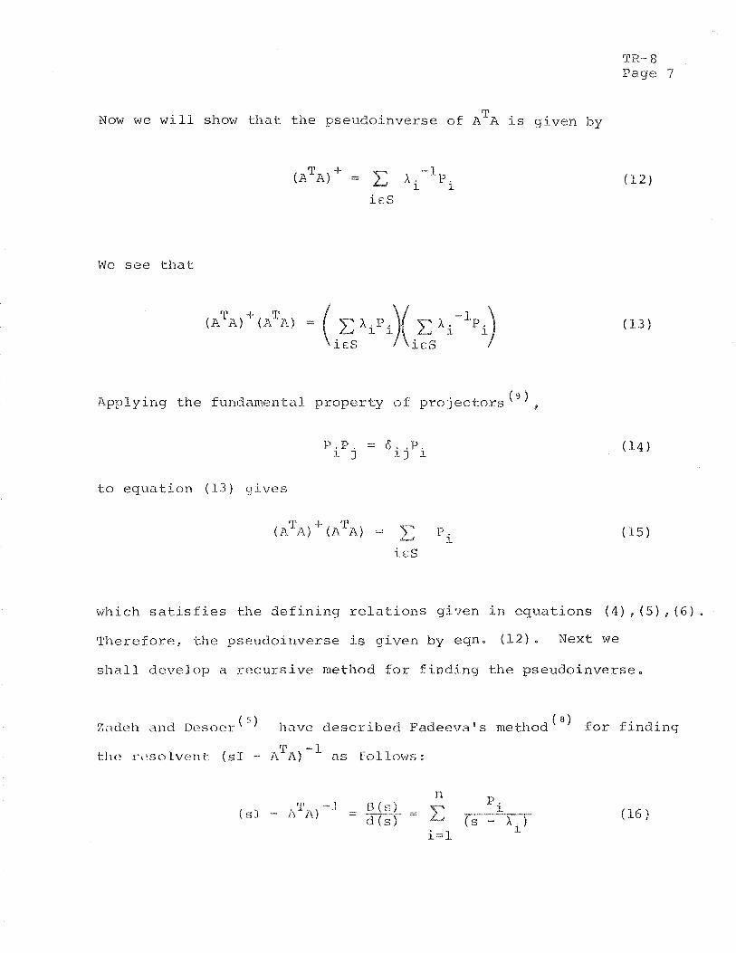
T NOW we will show that the pseudsinverse of A A is given by
We see that
( 9 ) Applying the fundamental property of projectors
P . P = 6 . " P 1 j 5-1 i
to equation (13) g i v e s
which satisfies the defining relations given in equations (4) (5) (6)
Therefore, the pseudsinverse is given by eqn, ( 1 2 ) . Next we
shall develop a recursive method for finding the pseudoinverse.
Zadch <ind Dcsoe~- ( have described Fadecva's method ( " for finding 'P - 1
t l ~ c . r t ~ s o l v c ~ t l t ( S T - A"A) as follows:
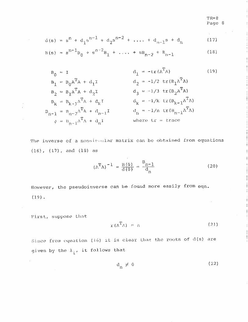
TR- 8 P a g e 8
T BO = 1 d, = - t r ( A A )
T T BL = BOA A + d l I d, = - 1 / 2 t r ( B I A A )
T T B2 - BIA A + d g d3 = -1/3 t r ( B 2 A A )
- T Bk - Bk-lA A + d k l dk = - l / k ~ ~ ( B ~ - ~ A ~ A )
- - T A A + C I ~ - _ ~ I d n = - l / n ~ ~ ( B , - ~ A ~ A )
B1l- 1 Bn- 2
w h e r e t r = trace 11 - 1.
'The i n v e r s e of a noras in . :Lar m a t r i x can be ob t a ined f r o m equa t i ons
( 1 6 ) , (17), and ( 1 6 ) as
H o w e v e r , t h e pseudoinverse can be found m o r e e a s i l y f r o m eqn.
( 1 9 ) .
F i r s t , suppose t h a t
Since f rom t lyuat ion ( 1 6 ) i t is c lear t h a t thc roots of d ( s ) a r e
g iven by t h e h i , it f o l l o w s t h a t
an t' 0 ( 2 2 )
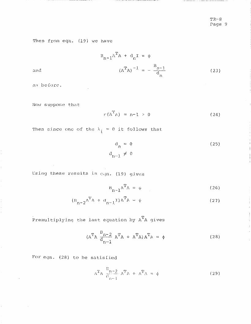
TR- 8 Page 9
Then from eqn. (2-9) we have
Now suppose tl1a t
?' r ( R A) = n-l > Q
Then since one of the h = O it follows that i
Using these results in c q n , (19) gives
T Premultiplying the last equation by A A gives
(il A -- T T A ~ A + n A j A A = + dn- l
For eqn. (28) to be satisfied
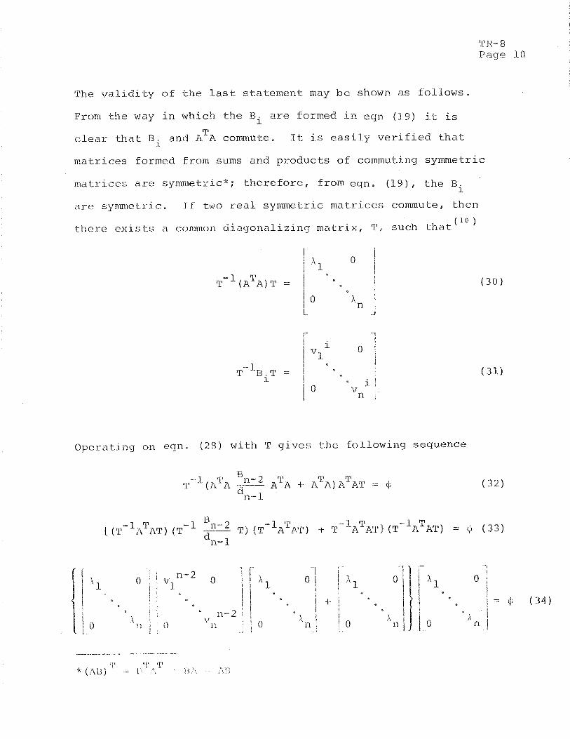
TR- 8 Page LO
The validity of t h e l a s t s t a t e m e n t may b e shown as f o l l o w s ,
From t h e way i n which t h e Bi a r e formed i n eqn (19) i t i s
T c l e a r t h a t Bi and A F, commute. It i s e a s i l y v e r i f i e d t h a t
m a t r i c e s formed from sums and p r o d u c t s o f commuting symmetric
m a t r i c e s a re symmetric*; t h e r e f o r e . f rom eqn. ( 1 9 ) , t h e B~
a r c synunctr ic , I f two r e a l symmetric m a t r i c e s commute, t h e n
t l ~ c r c e x i s t s n conunon c l i ayona l i z ing m a t r i x , T , such t h a t ( l o 1
Opcrntiilcj on eqn , (28) w i t h T g i v e s t h e f o l l o w i n g sequence
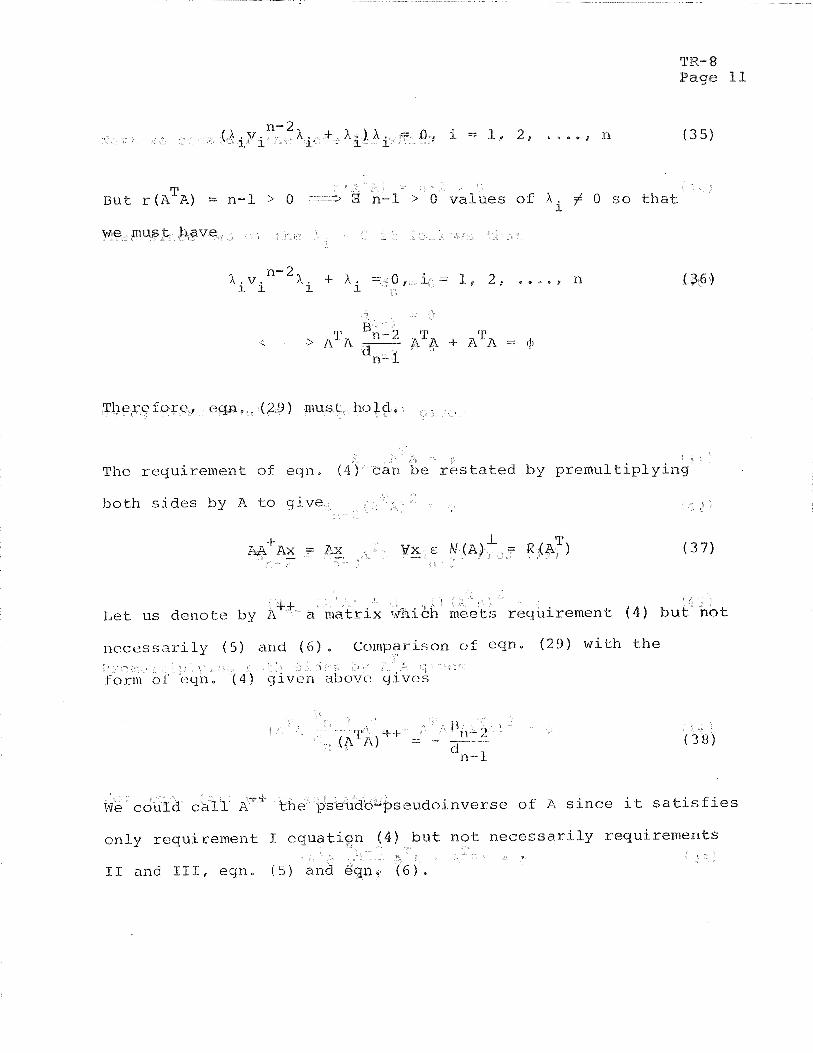
TI?-- 8 Page 11
T But r ( A A) = n-1 > 0 I s o f X i $ 0 s o t h a t
w e must ha
T h c l - c eqn, ( 2 9 ) must h o l d .
The r e q u i r e m e n t of e q n , ( e r e s t a t e d by p r e m u l t i p l y i n
b o t h s i d e s by A t o g i v e
( 3 7 )
L e t us d e n o t e by i x r e q u i r e m e n t ( 4 ) bu t
l i ccess r r r i ly ( 5 ) and ( 6 ) . Comparison o: eqn. ( 2 9 ) w i t h t h e
4-4- A t h s e u d o i n v e r s e o f A s i n c e i t s a t i s f i e s
o n l y r e q u i r e m e n t 1 e n e c e s s a r i l y r e q u i r e m e n t s
I1 and 111, eqn . ( 5 )
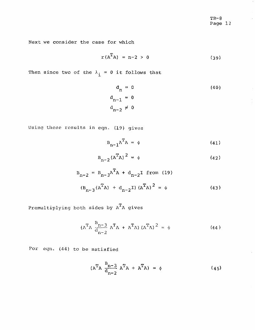
TR- 8 Page 12
Next we cons ider t h e case f o r which
Then s i n c e two of t h e h i = 0 it follows t h a t
Us ing t h e s o results in eqn, (19) gives
- T Bn- 2 - Bn-3 A A + dn-21 from (19)
T Premultiplying both s i d e s by A A g ives
F o r eqn. ( 4 4 ) t o be s a t i s f i e d
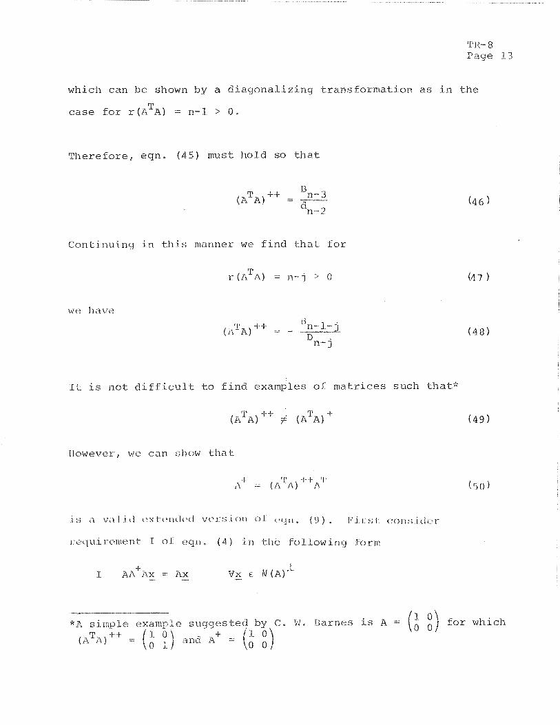
TR- 8 Page 1 3
which can be shown by a d i agona l i z ing t r ans fo rma t ion a s i n t h e
T ca se f o r r ( A A ) = n-1 > 0 .
The re fo re , egn. ( 4 5 ) must hold so that
Continuing i n t h i s manner we f i n d t h a t f o r
T r(A A ) = n- j > 0
++ - ( i l ' ~ ) - Bn-l- j- D n - j
I t i s no t d i f f i c u l t t o f i n d examples of ma t r i ce s such that*
Ilowevcr, we can show t h a t
I :; , I ",I 1 i t i clxt c - n t i c ~ i vtxr-:; i o l l ol- t ' ( j l i . ( 0 ) leij r;;L C O I ~ : ; iclc-r
1-c.c1ui1-cint?nt T of cqn, ( 4 ) i n t h e fo l lowing form
e sugges t e f o r which and A' =:
1 0 0 0
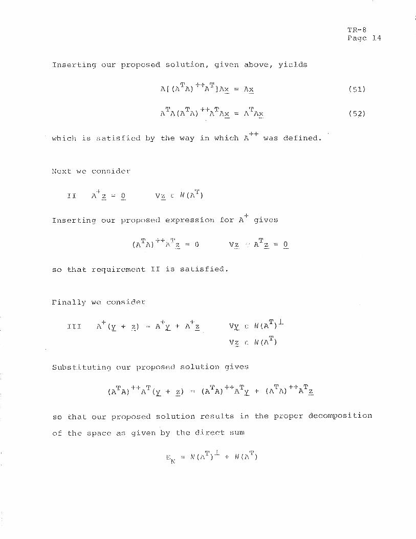
TIP- 8 Page 1 4
I n s e r t i n g o u r p r o p o s e d s o l u t i o n , g i v e n above , y i e l d s
A[ ( A ~ A ) + + A ~ I A ~ = AX -
T A ~ A ( A ~ A ) + + A ~ A ~ - = A AX -
4-4- which i s s a t i s f i e d by t h e way i n which A was d e f i n e d ,
Next w e c o n s i d e r
+ I n s e r t i n g o u r p r o p o s e d e x p r e s s i o n f o r A g i v e s
s o t h a t r e q u i r e m e n t I1 i s s a t i s f i e d ,
F i n a l l y w e c o n s i d e r
S u b s t i t u t i n g o u r p roposed s o l u t i o n g i v e s
4-4- T (3~) n (x + z) = ( A ~ A ) + + A ~ ~ + m T ~ ) + + n T z -
so t h a t o u r p r o p o s e d s o l u t i o n r e s u l t s i n t h e p r o p e r d e c o m p o s i t i o n
o f t h e s p a c e a s g i v e n by t h e d i r e c t sum
EN - k ( A T j L + N ( A ~ )
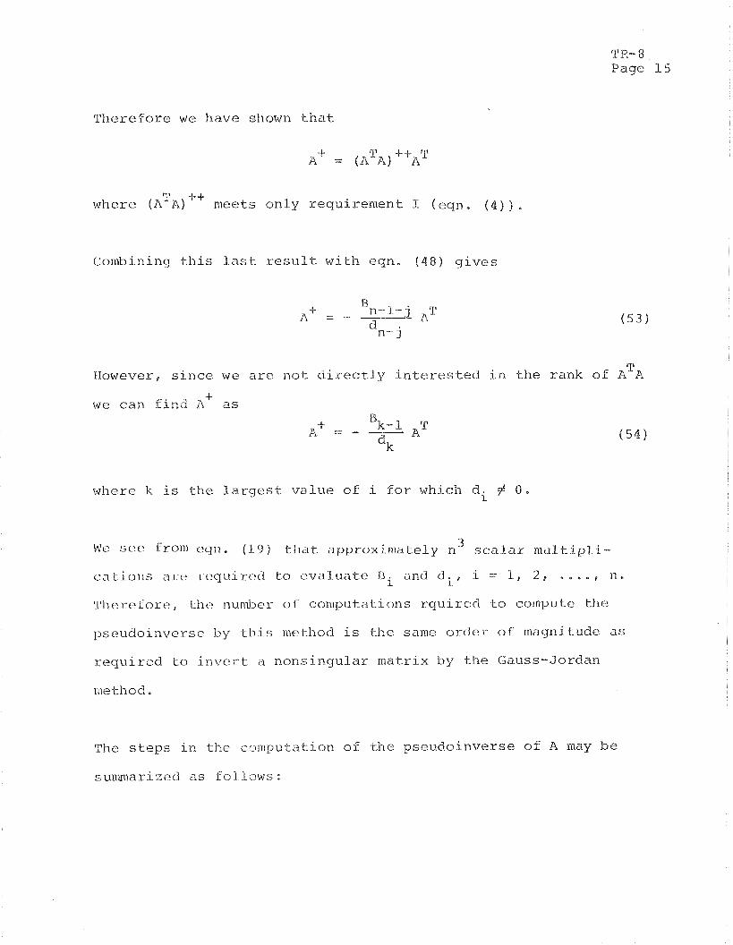
TR- 8 Page 15
T h e r e f o r e w e h a v e shown t h a t
C A = (A~A)
T where ( A A)" m e e t s o n l y r e q u i r e m e n t 1 ( e q n . ( 4 ) ) .
Conxb in in~ t h i s l a s t r e s u l t w i t h e q n . ( 4 8 ) g i v e s
£Iowever, s i n c e w e a r e n o t d i r e c t l y i n t e r e s t e d i n t h e r a n k o f A"A
-t- w e c a n f i n d A a s
where k is the l a r g e s t v a l u e o f i f o r which di f 0 ,
hJe see fro111 ~ ( 1 1 1 . ( 1 9 ) t h a t i l pp rox ima te ly n 3 sca lar m u l t i p l i -
c c l t i o ~ i s a r e r e q u i u ~ c l t o C : V ~ ~ U ~ I ~ C B and. dip i = I , 2 , - , , . , n, i
T l l c r c f o r e , thc nunber o f c o m p u t a t i o n s rc luire t l t o compuk~: thc?
p s e u d o i n v c r s e by t h i s methoci is t h e same o r d e r of magni tude a s
r e q u i r e d t o i n v e r t a n o n s i n g u l a r m a t r i x by t h e Gauss-Jordan
The s t e p s i n t h e c o m p u t a t i o n o f the p s e u d o i n v e r s e o f A may be
sumn~arizt?c$ as foi lows :

TR- 8 Page 16
T 1. Form A A
2- Compute B . , d., i = 1, 2 , . . . . , n from eqn, (19) L 1.
3 . F i n d k as t h e largest i for which di f 0
4, Compute the pseudoinverse of A from c q n . ( 5 4 )
TR- 8 Page 17'
Exampbe Problem
The a lgor i thm desc r ibed by t h i s paper for f i n d i n g t h e pseudo-
i n v e r s e h a s been p rog ramed i n BASIC a s shown by t h e f l o w
diagram of F ig , TR-8-1 and a s s o c i a t e d program l i s t i n g . This
program has been t e s t e d us ing the example problem g iven by
G r e v i l l e with r e s u l t s a s shown i n Table TR-8-1. These
r e s u l t s a r e i n agreement w i th t h o s e ob ta ined by Grevi lPe.
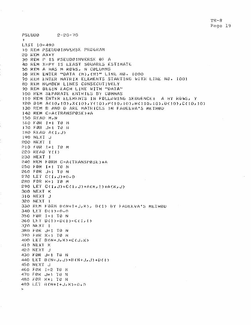
TR-8 Page 19
PSEbB9 2-20- 70 0
L I S T HO-490 aa R E M PsEuDtaarJvEl isE P K G G I ~ A M z0 REB AX=.f 30 REM P 1s PSEUUQINVERSE @ b U 40 RLM X = P Y IS LEAST S Q U A R L S ESTPMATL 50 HEM A HAS M H 8 k S s N CULOMNS 60 REM ENTER '"DATA dM)sCN16' LPNC N@e l0OQ 30 HEM ENTLK MATRIX ELkNENTS S T A f < T I N G kITW L I N k & O e 1001 &O REM NUMBER LIMES C B N S E C b T I L L L Y 30 REM B E G I N t A G H L I N E k l T H '@DATAss 100 REM SLPAHATE E-N?HILS BY CGMMAS I f 0 R E M ENTER kLEiV)CNTS 1M F@LLWI*IXPJb SEQUENCL: A B Y R O ~ S J V 120 DIM ACl0~10)aXClO),YClO)aPf1Q)s 1 0 9 ~ B C f I I ~ ~ ~ ~ C C ~ B D ~ ~ O ~ ~ C ~ ~ Q ~ 801 $30 REM B AN13 D AKt M A T K I C k S I N r "AL ) tE \ rAwS PIC'FHBLI 140 REM C=ACTRANSPOSF)*A t 5 0 READ M,Pd 140 FBM P = 1 TU Pi 170 FBR J= l T d N 1 S 0 h k A 0 A C I a J ) i 9 O NLXT 4 200 NEXT I 210 F U R % = f T@ M 220 READ Y C I ) 230 NEXT I 240 REM FBWM C=ACTKAMSP@SL)*A 2 5 0 F B R I=l 40 N 260 FWK J = 1 1 W N 270 LET C C l s J ) = 6 * 0 280 FBH K=B T B M 290 LET C ~ Z B J ) = G ( I = J > + ~ C K ~ l > * P C K z J ) 300 NEXT K 310 NEXT J 320 NEXT I 330 Rid.M t 0 K M P C N * I + J , K ) j D < I $ f3Y P A U C L V A Q MMtlHVlh) 3 4 6 LFT D C I )=O.O 350 F @ K P = l TO N 360 L E I 0 C 1 ) = i ) ( f ) - [ J d l a I S 370 N k X f 1 3HI) k t 3 K .I= I 3°C) N 390 b d l < K=l 1k3 N 400 L L T R < N + J t K ) = C C J p K ) 410 NLXI' D(
420 NEXT J 430 F'@H J= l T O N 440 LET B(N+JaJ)=BQM+J,J)+D<l3 4 5 6 NEXT J 460 F @ R 2=2 TjL1 N 4'70 F @ H J= 1 Ti3 N 480 F O R K = f I B N 490 t E l B ( N * l + J s K ) = O e f l >
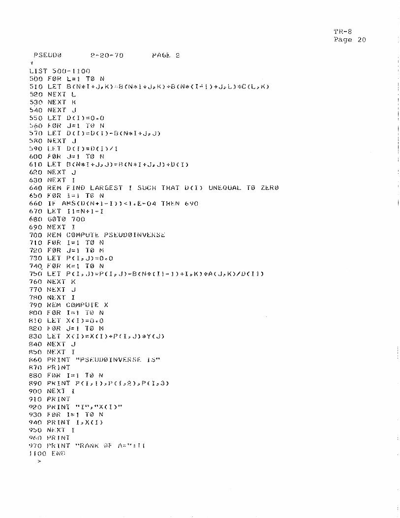
TR-8 Page 20
PSEUUa 2-20- 7 0 PAGL 2 P
L I S T 500-1100 500 C B H L = 1 T O N 510 LET B C N * I + , i s K " r - i 3 : " N ~ I + J ~ K l + B C E . i ~ a " I - I I + J > L " r * G 9 k s K I 520 N E X T L 530 NEXT K 540 N E X T J 550 LET U C I ) = O * O 5 6 0 b O K J = l Tt3 N 550 L.ET I ) < I B = I U ~ I ~ - R I N * I + 4 s JT 580 NkX'K J 590 L k T D < I ) = D < I ? / I 600 F 81.C ,I= 1 T13 N 610 L E T D<N*I+JDJ)=B<N*I+JIJ~+DCII 620 N E X T J 630 NF'X'I; I 640 REM F l N D LARGEST I SUCH THAT D < I l U N k Q U A L TB Z L M B 650 F O R I = 1 70 N 660 IC A B S C L t ( l V + I - I ) ) < I B E - 0 4 THLN 6 9 0 670 L E T II=N+l-B 680 G B T a 700 690 N E X T I 700 K E M CBMPUTk P S C U D B I N V L K Y L 710 F U R I = l T@ N 720 FBR J=i TO PI 730 L E T P ( l r J I = O e O 74q FOP K=f T B N 750 L E T PCP3 J > = P < I s J ) - B < N * E : E j - l l + % s K ) * A < d a K 3 / u ( I 1 ) 760 N E X T K 770 P J t X T J 780 N E X T II 730 H t M [email protected] X ROO F O R I = l 1W N 810 LET X g I ) = O * O 820 t B R 2-1 10 M 830 L E T X C I I = X C I ~ + P < I S J ) * Y < J ) 840 N E X T J 850 NEXT I $460 PK INT ""PSEUOB I N V E H S L lS" 6 7 0 P R I N T SE3O F@R I = ! TO N 890 P R I N T P < I t f 9 a P < I a 2 ) ~ ? < 1 1 @ ) 800 NEXT I 810 PKIM1' "20 P R I N T ' ' 1 5 v 9 ' * X < I l e v 930 F B R I I = P TB N 940 P R I N T I s X C I 3 950 I\IE.XT P o6O P R I N T '370 b'l$ I N 1 "RbNk ( T i - R-." ": 1 1 i OO ENL)
>
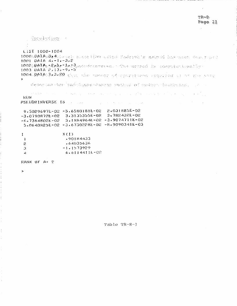
TR-8 Page 2 1
I X ( I 3 1 e 901 H4433 2 e 640356116 3 - 1 e 1573929 4 6 . 6 1 1 4 4 l l L - 0 2
HANK rBF A = 2

TR- 8 Page 22
Conclusion
A computational algorithm using FadeevaPs method has been described
for finding the pseudoinverse, The method is computationally
efficient in that the number of operations required is of the same
order as for the Gauss-Jordan method of matrix inversion.

TR- 8 Page 2 3
Acknow ledaements
The a u t h o r wishes t o thank P r o f , David I s a a c s (Un ive r s i t y of
C a l i f o r n i a , I r v i n e ) f o r p o i n t i n g o u t the work done by G r e v i l l e
I a m p a r t i c u l a r l y g r a t e f u l t o P r o f , C, W, Barnes (Un ive r s i t y o f
C a l i f o r n i a , I r v i n e ) f o r p o i n t i n g o u t t h e power of p r o j e c t o r s i n
m a t r i x a n a l y s i s and f o r d e t e c t i n g an e r r o r i n an ear l ier d r a f t
of t h i s paper ,
TR- 8 Page 2 4
B ib -
( " ~ r e v i l l e . T. N. E. , 'The P s e u d o i n v e r s e o f a R e c t a n g u l a r o r
S i n g u l a r M a t r i x a n d i t s A p p l i c a t i o n t o t h e S o l u t i o n o f S y s t e m s
o f L i n e a r E q u a t i o n s , " SIW Review, Vo l . 1, N o , 1, J a n , 1959 ,
pp, 38-43.
( D e u t s c h , R a l p h , P r e n t i c e - H a l l , 1965 ,
p p , 82-89,
( 3 ) ~ o k i , Mansanao, O p t i m i z a t i o n o f S t o c h a s t i c Sys t em, Academic
P r c s s , 1967 , pp. 3 1 8 - 3 2 4 ,
( ' ) Zadch, L o f t i A., Desoer, C h a r l e s A . , I
M c G r a w - H i l l , 1 9 6 3 , pp- 577-582
( ) Freedman, B e r n a r d ,
P . la themntics , W i l e y , 1956 . -- -
( ' 1 - 1 , 1,. C , - L i n t \ n ~ - - - -- - - -- A a f o r Undc ' rgrndui i tcs , Wi l e y , 1957 .
( " ~ a d c e v a , V e N a , - C o n l p u t a t i ~ n a l Methods i n L i n e a r A l g e b r a , Dover ,
1 9 59.
TR- 8 Page 2 5
( ' 'pease, Harshall C . , Methods o f Matrix Algebra, Academic
Press , 1 9 6 5 .
I ' lo ' Bellman, Richard, McGraw-Hill,

APPENDIX INTIIODUCTIBN
The f o l l o w i n g e i g h t T e c h n i c a l Repor t s w e r e w r i t t e n by John Kinke l
i n r e s p o n s e t o a n ass ignment t o i n v e s t i g a t e t h e proposed methods
o f c l o s e d - l o o p i o n o s p h e r i c d a t a r e d u c t i o n and p r o v i d e t h e mathe-
m a t i c a l p r o o f s n e c e s s a r y f o r a s o l i d t h e o r e t i c a l f o u n d a t i o n ,
TR-1 "Some Proposed Methods f o r Reduct ion o f Topside Ionograms
t o E l e c t r o n D e n s i t y P r o f i l e s "
Methods a r e d e s c r i b e d f o r f i n d i n g N ( h ) o r N ( h , t) from
t o p s i d e ionograms u s i n g approx imat ion t h e o r y . A g r a d i e n t
t e c h n i q u e is proposed t o f i n d t h e p a r a m e t e r s of t h e
approx imat ing f u n c t i o n ,
TR-2 "A Weighted L e a s t Squares Approximation Methodq'
The t h e o r y of M a l l i n c k r o d t b we igh ted l e a s t s q u a r e s
approx imat ion method i s i n v e s t i g a t e d .
TR-3 " I n v e r s e Mapping t o S p e c i f i e d f "
A r ~ t c t l ~ o c i i s dcveloycd f o r computing v a l u e s of H{T,(x) -
a t t l ~ c same f requency a s scalecl data. p o i n t s i n t h e h q f )
p l ane ,
TR-4 "Simplification of Matrix Inversion Problem"
A method is developed for solving fox - X in the matrix
equation AX - = - B, without computing A - ' ~
TR-5 "Time Skew Problem"
The time skew problem in Horizontal Processing is
investigated.
TR-6 "Optimal Step Size by One Dimensional Search"
A method is developed for optimizing the step size of a
hyper-dimensional adjustment vector that is used in the
matrix method.
TR-7 "Horizontal Processing"
Some of the considerations in Horizontal Processing are
investigated,
TR-8 "Computation of the Pseudoinverse"
The development and proof of a new computational algorithm
for constructing the pseudoinverse sf a matrix is given,