C

n

Ia

b

c

h

����

a

ARRA

KOPGNSDSS

1

ticrot

0h

Journal of Neuroscience Methods 211 (2012) 245– 264

Contents lists available at SciVerse ScienceDirect

Journal of Neuroscience Methods

jou rna l h om epa ge: www.elsev ier .com/ locate / jneumeth

omputational neuroscience

STAT: Open-source neural spike train analysis toolbox for Matlab

. Cajigasa,b,c,∗, W.Q. Malika,c, E.N. Browna,b,c

Department of Anesthesia and Critical Care, Massachusetts General Hospital, Harvard Medical School, Boston, MA 02114, United StatesHarvard-MIT Division of Health Sciences and Technology, Massachusetts Institute of Technology, Cambridge, MA 02139, United StatesDepartment of Brain and Cognitive Sciences, Massachusetts Institute of Technology, Cambridge, MA 02139, United States

i g h l i g h t s

We have developed the neural spike train analysis toolbox (nSTAT) for Matlab®.nSTAT makes existing point process/GLM methods for spike train analysis more accessible to the neuroscience community.nSTAT adopts object-oriented programming to allow manipulation of data objects rather than raw numerical representations.nSTAT allows systematic building/testing of neural encoding models and allows these models to be used for neural decoding.

r t i c l e i n f o

rticle history:eceived 15 January 2012eceived in revised form 6 August 2012ccepted 7 August 2012

eywords:pen-sourceoint processeneralized linear modelseurosciencetatisticsata analysisignal processingpike trains

a b s t r a c t

Over the last decade there has been a tremendous advance in the analytical tools available to neuro-scientists to understand and model neural function. In particular, the point process – generalized linearmodel (PP-GLM) framework has been applied successfully to problems ranging from neuro-endocrinephysiology to neural decoding. However, the lack of freely distributed software implementations of pub-lished PP-GLM algorithms together with problem-specific modifications required for their use, limit wideapplication of these techniques. In an effort to make existing PP-GLM methods more accessible to theneuroscience community, we have developed nSTAT – an open source neural spike train analysis tool-box for Matlab®. By adopting an object-oriented programming (OOP) approach, nSTAT allows users toeasily manipulate data by performing operations on objects that have an intuitive connection to theexperiment (spike trains, covariates, etc.), rather than by dealing with data in vector/matrix form. Thealgorithms implemented within nSTAT address a number of common problems including computation ofperi-stimulus time histograms, quantification of the temporal response properties of neurons, and char-

acterization of neural plasticity within and across trials. nSTAT provides a starting point for exploratorydata analysis, allows for simple and systematic building and testing of point process models, and fordecoding of stimulus variables based on point process models of neural function. By providing an open-source toolbox, we hope to establish a platform that can be easily used, modified, and extended by thescientific community to address limitations of current techniques and to extend available techniques tomore complex problems.

. Introduction

Understanding and quantifying how neurons represent andransmit information is a central problem in neuroscience. Whethert involves understanding how the concentration of a particularhemical present within the bath solution of an isolated neu-on affects its spontaneous spiking activity (Phillips et al., 2010)

r how a collection of neurons encode arm movement informa-ion (Georgopoulos et al., 1986), the neurophysiologist aims to

∗ Corresponding author. Tel.: +1 617 407 3367.E-mail address: iahn@mit.edu (I. Cajigas).

165-0270/$ – see front matter © 2012 Elsevier B.V. All rights reserved.ttp://dx.doi.org/10.1016/j.jneumeth.2012.08.009

© 2012 Elsevier B.V. All rights reserved.

decipher how the individual or collective action potentials of neu-rons are correlated with the stimulus, condition, or task at hand.

Due to the stereotypic all-or-none nature of action potentials,neural spiking activity can be represented as a point process, a timeseries that takes on the value 1 at the times of an action potentialand is 0 otherwise (Daley and Vere-Jones, 1988). Many other com-mon phenomena can be described as point processes ranging fromgeyser eruptions (Azzalini and Bowman, 1990) to data traffic withina computer network (Barbarossa et al., 1997). Generalized linearmodels (GLMs) (McCullagh and Nelder, 1989), a flexible generaliza-

tion of linear regression, can be used in concert with point processmodels to yield a robust and efficient framework for analyzing neu-ral spike train data. This point process – generalized linear model(PP-GLM) framework has been applied successfully to a broad range

2 scienc

oe2(eaSTo

aupapppwotat

pisM(psadatFaoscfat

cTeyrcmsnotma

PsiamtbOm

46 I. Cajigas et al. / Journal of Neuro

f problems including the study of cardiovascular physiology (Chent al., 2011, 2010a,b, 2008b, 2009a, 2008a; Barbieri and Brown,004, 2006a,b; Barbieri et al., 2005a), neuro-endocrine physiologyBrown et al., 2001), neurophysiology (Schwartz et al., 2006; Frankt al., 2002, 2004, 2006; Eden et al., 2004b; Vidne et al., 2012),nd neural decoding (Barbieri et al., 2004, 2008; Eden et al., 2004a;rinivasan et al., 2006, 2007; Wu et al., 2009; Ahmadian et al., 2011).ruccolo et al. (2005) and Paninski et al. (2007) provide a broadverview of the PP-GLM framework.

While much progress has been made on the developmentnd application of PP-GLM methods within neuroscience, these of these methods typically requires in-depth knowledge ofoint process theory. Additionally, while there are widely avail-ble implementations for the estimation of GLMs within softwareackages such as Matlab® (The Mathworks, Natick, MA), S, or Rrogramming languages, their use to analyze neural data requiresroblem specific modifications. These adaptations require muchork on the part of the experimentalist and detract from the goal

f neural data analysis. These barriers are exacerbated by the facthat even when software implementations are made publicly avail-ble they vary greatly in the amount of documentation provided,he programming style used, and in the problem-specific details.

Numerous investigators have successfully addressed commonroblems within neuroscience (such as spike sorting, data filter-

ng, and spectral analysis) through the creation of freely availableoftware toolboxes. Chronux (Bokil et al., 2010), FIND (previouslyEA-Tools) (Meier et al., 2008; Egert et al., 2002), STAToolkit

Goldberg et al., 2009), and SPKtool (Liu et al., 2011) are a few exam-les of such tools. Chronux offers several routines for computingpectra and coherences for both point and continuous processeslong with several general purpose routines for extracting specifiedata segments or binning spike time data. STAToolkit offers robustnd well-documented implementations of a range of information-heoretic and entropy-based spike train analysis techniques. TheIND toolbox provides analysis tools to address a range of neuralctivity data, including discrete series of spike events, continu-us time series and imaging data, along with solutions for theimulation of parallel stochastic point processes to model multi-hannel spiking activity. SPKtool provides a broad range of toolsor spike detection, feature extraction, spike sorting, and spike trainnalysis. However, a simple software interface to PP-GLM specificechniques is still lacking.

The method for data analysis within the PP-GLM framework isonsistent and amenable to implementation as a software toolbox.here are two main types of analysis that can be performed: (1)ncoding analysis and (2) decoding analysis. In an encoding anal-sis, the experimenter seeks to build a model that describes theelationship between spiking activity and a putative stimulus andovariates (Paninski et al., 2007). This type of analysis requiresodel selection and assessing goodness-of-fit. A decoding analy-

is estimates the stimulus given spiking activity from one or moreeurons (Donoghue, 2002; Rieke, 1999). An example of this typef analysis would aim to estimate arm movement velocity givenhe population spiking activity of a collection of M1 neurons and a

odel of their spiking properties such as that developed by Morannd Schwartz (1999).

We use the consistency of the data analysis process within theP-GLM framework in the design of our neural spike train analy-is toolbox (nSTAT). Our object-oriented software implementationncorporates knowledge of the standard encoding and decodingnalysis approaches together with knowledge of the common ele-ents present in most neuroscience experiments (e.g. neural spike

rains, covariates, events, and trials) to develop platform that cane used across a broad range of problems with few changes.bject-oriented programming (OOP) represents an attempt toake programs more closely model the way people think about

e Methods 211 (2012) 245– 264

and interact with the world. By adopting an OOP approach for soft-ware development we hope to allow the user to easily manipulatedata by performing operations on objects that have an intuitiveconnection to the experiment and hypothesis at hand, rather thanby dealing with raw data in matrix/vector form. Building the tool-box for Matlab®, we make sure that users can easily transfer theirdata and results from nSTAT to other public or commercial soft-ware packages, and develop their own extensions for nSTAT withrelative ease.

nSTAT address a number of problems of interest to the neuro-science community including computation of peri-stimulus timehistograms, quantification of the temporal response properties ofneurons (e.g. refractory period, bursting activity, etc.), character-ization of neural plasticity within and across trials, and decodingof stimuli based on models of neural function (which can be pre-specified or estimated using the encoding methods in the toolbox).Importantly, the point process analysis methods within nSTAT arenot limited to sorted single-unit spiking activity but can be appliedto any binary discrete spiking process such as multi-unit thresholdcrossing events (see for example Chestek et al., 2011). It should benoted that while all of the examples presented in the paper focuson the PP-GLM framework, nSTAT contains methods for analyz-ing spike trains when they are represented by their firing rate andtreated as a Gaussian time-series instead of a point process. Theseinclude time-series methods such as Kalman Filtering (Kalman,1960), frequency domain methods like multi-taper spectral estima-tion (Thomson, 1982), and mixed time-frequency domain methodssuch as the spectrogram (Cohen and Lee, 1990; Boashash, 1992).For brevity, and because these methods are also available in othertoolboxes, we do not discuss these elements of the toolbox herein.

This paper is organized as follows: Section 2.1 summarizes thegeneral theory of point processes and generalized linear modelsas it applies to our implementation. We include brief descriptionsof some of the algorithms present in nSTAT to establish consistentnotation across algorithms developed by distinct authors. Section2.2 describes the software classes that make up nSTAT, the relation-ships among classes, and relevant class methods and properties.Section 2.3 describes five examples that highlight common prob-lems addressed using the PP-GLM framework and how they canbe analyzed using nSTAT. Lastly, results for each of the differ-ent examples are summarized in Section 3. nSTAT is available fordownload at http://www.neurostat.mit.edu/nstat/. All examplesdescribed herein (including data, figures, and code) are containedwithin the toolbox help files. The software documentation alsoincludes descriptions and examples of the time-series methods notdiscussed herein for brevity.

2. Materials and methods

2.1. Summary of the PP-GLM framework

In this section, we describe the PP-GLM framework and themodel selection and goodness of fit techniques that can be appliedwithin the framework to select among models of varying com-plexity. The peri-stimulus time histogram (PSTH) and its PP-GLManalogue, the GLM-PSTH, are then presented together with exten-sions that allow for estimation of both within-trial and across-trialneural dynamics (SSGLM). We then discuss how point processmodels can be used in decoding applications when neural spikinginformation is used to estimate a driving stimulus.

2.1.1. Point process theoryDue to the stereotyped all-or-none nature of action potentials,

neural spiking activity can be represented as a point process, i.e.as a time series that takes on the value 1 at the time of an action

scienc

pabi(

�

w�sco

uvrrotIis

2

ism(rarlswtcpi

a

l

ata

l

wo�a

o

2

ieatt

I. Cajigas et al. / Journal of Neuro

otential and is 0 otherwise. Given an observation interval (0, T] and time t ∈ (0, T], we define the counting process N(t) as the total num-er of spikes that have occurred in the interval (0, t]. A point process

s completely characterized by its conditional intensity functionCIF) (Daley and Vere-Jones, 1988) defined as

(t|Ht) = lim� → 0

Pr(N(t + �) − N(t) = 1 | Ht)�

(1)

here Ht is the history information from 0 up to time t. For any finite, the product �(t|Ht)� is approximately the probability of a single

pike in the interval (t, t + �] given the history up to time t. Theonditional intensity function can be considered a generalizationf the rate for a homogeneous Poisson process.

If the observation interval is partitioned into {tj}Jj=0 and individ-

al time steps are denoted by �tj = tj − tj−1, we can refer to eachariable by its value within the time step. We denote Nj = N(tj) andefer to �Nj = Nj − Nj−1 as the spike indicator function for the neu-on at time tj. If �tj is sufficiently small, the probability of more thanne spike occurring in this interval is negligible, and �Nj takes onhe value 0 if there is no spike in (tj−1, tj] and 1 if there is a spike.n cases where fine temporal resolution of the count process, N(t),s not required we define �N(tA, tB) to equal the total number ofpikes observed in the interval (tA, tB].

.1.2. Generalized linear modelsThe exponential family is a broad class of probability models that

nclude many common distributions including the Gaussian, Pois-on, binomial, gamma, and inverse Gaussian distributions amongany others. The key concept underlying generalized linear models

GLMs) (McCullagh and Nelder, 1989) involves expressing the natu-al parameter of the probability model from the exponential familys a linear function of relevant covariates. Efficient and robust algo-ithms for linear regression can then be employed for maximumikelihood parameter estimation. Thus if the conditional inten-ity function is modeled as a member of the exponential family,e have an efficient algorithm for estimating CIF model parame-

ers. Additionally, this approach allows effective selection betweenompeting models via the likelihood criteria described below. Inarticular, we will use two main types of GLMs for the conditional

ntensity functions herein:(1) Poisson regression models where we write log(�(tj|Htj

)�) as linear function of relevant covariates, e.g.

og(�(tj|Htj)�) = xT

j ̌ (2)

nd (2) binomial regression models where we write the inverse ofhe logistic function, logit(�(t|Ht)�), as a linear function of covari-tes, e.g.

ogit(�(tj|Htj)�) = xT

j ̌ (3)

here xTj

is the jth row of the design matrix X and ̌ is the vectorf model parameters to be estimated. The spike indicator function,Nj, is taken as the observation, termed yj, and is modeled either as

Poisson or binomial random variable. That is yj = �Nj∼ exp(xTjˇ)

r yj∼exp(xT

jˇ)

1+exp(xTj

ˇ).

.1.3. Model selectionGoodness of fit measures currently implemented in nSTAT

nclude the time rescaling theorem for point processes (Brown

t al., 2002), Akaike’s information criteria (AIC) (Akaike, 1973),nd Bayesian information criteria (BIC) (Schwarz, 1978). Briefly,he time rescaling theorem states that given the true condi-ional intensity function of a point process, �, and a sequence of

e Methods 211 (2012) 245– 264 247

spike times 0 < t1 < t2 < . . . < ts < . . . < tS < T, the rescaled spike timesdefined as

us = 1 − exp(

∫ ts

ts−1

�(�|H�)d�) (4)

where s = 1, . . ., S are independent, identically distributed, uniformrandom variables on the interval (0, 1). To use the time-rescalingtheorem to test model goodness of fit, one can apply Eq. (4) to eachcandidate model, �i, to obtain a set of candidate rescaled spike timesui

s that can then be tested for independence and their closeness (tobe made precise below) to an uniform distribution.

The Kolmogorov–Smirnov (KS) test can be used to comparehow close the empirical distribution of rescaled spike times, us’s,are to a reference uniform distribution on the interval (0, 1). Thevisual representation of this test, termed a KS plot (Brown et al.,2002), together with corresponding confidence intervals (Johnsonand Kotz, 1970) allows for comparison of multiple models simulta-neously. If the candidate model is correct, the points on the KS plotshould lie on a 45◦ line (Johnson and Kotz, 1970). The KS statisticis the largest deviation from the 45◦ line. Application of the time-rescaling theorem to sampled data produces some artifacts withinKS plots since the actual spike times could have occurred anywherewithin the finite-sized time bins. These artifacts are addressedwithin nSTAT using the discrete time rescaling theorem (Haslingeret al., 2010).

Independence of the rescaled spike times can be assessed byplotting ui

s+1 vs. uis (Truccolo et al., 2005). In this case, a corre-

lation coefficient statistically different from zero casts doubt onthe independence of the rescaled spike times. A stronger test forindependence uses the fact that uncorrelated Gaussian randomvariables are also independent. If the ui

s’s are uniform random vari-ables on the interval (0, 1), then

xis = ˚−1(ui

s) (5)

where ˚−1(·) is the inverse of the standard normal distributioncumulative distribution function (CDF), will be normally dis-tributed with zero mean and unit variance. Significant non-zerocoefficients of the auto-correlation function of the xi

s’s at non-zerolags demonstrates that the rescaled spike times are not inde-pendent (Truccolo et al., 2005). The 95% confidence interval forthe non-zero lag coefficients of the auto-correlation function is±1.96/

√n where n is the total number of rescaled spike times.

Goodness of fit can also be assessed by examining the struc-ture of the point process model residuals (Andersen, 1997; Truccoloet al., 2005) defined over non-overlapping moving time windowsof size B as

Mij = M(tj) =

j∑n=j−B

�N(tn) −∫ tj

tj−B

�i(�|H�, �̂)d� (6)

for j − B ≥ 1. Strong correlations between covariates absent fromthe model for �i and Mi

jare indicative of potentially important un-

modeled effects.The AIC, BIC, rescaled spike times, and the point process resid-

uals are computed within the nSTAT Analysis class for eachcandidate model, �i, and stored within the returned FitResultobject (see Section 2.2 for more details). The FitResult methodplotResults displays the KS plot, the plot of ui

s+1 vs. uis and corre-

sponding correlation coefficient, the auto-correlation function ofthe xi

s’s, and the point process residual for each of the candidate�i’s.

2.1.4. Simulating point processesValidation and testing of new algorithms requires generat-

ing spiking activity according to known prior behavior. Given an

2 scienc

ice

123

456

Ine1sCat

2

saacPtsa1

sttbipt(G

l

fa

g

agTNswpieewbtbb

48 I. Cajigas et al. / Journal of Neuro

ntegrable CIF �(t|Ht) for 0 ≤ t ≤ T, a realization of the point processompatible with this CIF can be generated via time rescaling (Brownt al., 2002) as follows:

. Set t0 = 0; set s = 1.

. Draw zs an exponential random variable with mean 1.

. Find ts as the solution to zs =∫ ts

ts−1�(�|H�)d�.

. If ts > T, then stop.

. s = s + 1

. Go to 2.

n instances where the CIF is independent of history (e.g. a homoge-ous or inhomogenous Poisson process), the more computationallyfficient point process thinning algorithm (Lewis and Shedler,978; Ogata, 1981) can be used. The nSTAT CIF class containstatic methods (e.g. CIF.simulateCIF, CIF.simulateCIFByThinning, andIF.simulateCIFByThinningFromLambda) to generate a realization of

point process based on either time rescaling or the point processhinning algorithm.

.1.5. PSTH and the GLM frameworkIn neurophysiology, the peri-stimulus time histogram and post-

timulus time histogram, both abbreviated PSTH or PST histogram,re histograms of the times at which neurons fire. These histogramsre used to visualize the rate and timing of neuronal spike dis-harges in relation to an external stimulus or event. To obtain aSTH, a spike train recorded from a single neuron is aligned withhe onset, or a fixed phase point, of an identical repeatedly pre-ented stimulus. The aligned sequences are superimposed in timend then combined to construct a histogram (Gerstein and Kiang,960; Palm et al., 1988).

For concreteness, suppose that a PSTH is to be constructed frompiking activity of a neuron across K trials each of duration T. Theime interval T is partitioned into N time bins each of width � andhe spike trains represented by their value (0 or 1) within eachin. To estimate the firing rate via the PSTH, we partition the time

nterval T into R time bins (with T/R > �), sum the number of spikesresent across all trials within the each of the R time bins, and dividehe total counts by the bin width (T/R). According to Czanner et al.2008), the PSTH is a special case of the CIF defined by the followingLM

og(�(k, n�|�)�) =R∑

r=1

�rgr(n�) (7)

or k = 1, . . ., K and n = 1, . . ., N. Here k and n are the trial numbernd bin within a trial respectively, and

r(n�) ={

1 if n = (r − 1)NR−1 + 1, . . . , rNR−1

0 otherwise(8)

re the unit pulse functions in the observation interval (0, T] (e.g.1(n�) = 1 from n = 1, . . ., NR−1 and zero outside this time interval).his conditional intensity function is the same for all trials k = 1, . . , K.ote that since there are R unit pulse functions over the N observed

amples, the width of each unit pulse function is NR−1. For the bin inhich gr(n�) = 1, the spiking activity obeys a homogenous Poissonrocess with mean rate exp(�r)/�, and since the basis functions

n Eq. (8) are orthogonal, the values exp(�r)/� r = 1, . . ., R can bestimated independently of each other. The maximum-likelihoodstimate of exp(�r)/� is the number of spikes that occur in the bin inhich gr(n�) = 1, summed across all trials, and divided by the num-

er of trials and the bin width (e.g. equal to the value of the PSTH inhe rth time bin). Within nSTAT, the PSTH and the GLM-PSTH cane computed for any collection of neural spike trains (representedy the class nstColl) by specifying the bin width T/R. The GLM-PSTH

e Methods 211 (2012) 245– 264

routine (psthGLM method) also allows for the estimation of spikinghistory effect of the same form as described in Section 2.1.6.

2.1.6. State space GLM frameworkThe standard PSTH treats each trial as independent to produce

an estimate of the firing rate. In many experiments it is of interestto not only capture the dominant variation in firing rates withina trial, but also to examine changes from one trial to the next(for example to examine neural plasticity or learning). Czanneret al. (2008) formulated the state-space generalized linear model(SSGLM) framework to allow for this type of analysis. Briefly theSSGLM framework proposes that the CIF be modeled as

log(�(k, n�|�)�) =R∑

r=1

�k,rgr(n�) +J∑

j=1

�j�Nk(tn − tj−1, tn − tj)

(9)

where k is the current trial index and �Nk(tA, tB) equals the totalnumber of spikes observed in the interval (tA, tB] of the kth trial.The stochastic trial-to-trial dependence between the parameters�k = [ �k,1 . . . �k,r . . . �k,R ] is described by the random walk model

�k = �k−1 + �k (10)

for k = 1, . . ., K, where K is the total number of trials, �k is an R-dimensional Gaussian random vector with mean 0 and unknowncovariance matrix ˙. The initial vector �0 is also assumed to beunknown. Because the parameters �k and � j of the GLM and thecovariance parameter, ˙, of the random walk model are unknown,an iterative Expectation-Maximization algorithm (Dempster et al.,1977) is employed to estimate them.

The spike rate function on the interval [t1, t2] is defined as

(t2 − t1)−1k(t1, t2) = (t2 − t1)−1∫ t2

t1

�(k, �|�k, �, Hk,�)d� (11)

where k(t1, t2) corresponds to the expected number of spikesin the interval [t1, t2]. The corresponding maximum likelihoodestimate of the spike rate function is obtained by evaluating Eq.(11) with the estimated conditional intensity function. Confidenceintervals can be constructed via the Monte Carlo methods describedby Czanner et al. (2008). Statistical comparisons of the spike ratefunction between trials can be performed in order to examine expe-rience dependent changes or learning across trials. In particular,for a given interval [t1, t2] and trials m and k we can compute themaximum-likelihood estimates of Eq. (11) and use Monte Carlomethods to compute

Pr[(t2 − t1)−1̂m(t1, t2) > (t2 − t1)−1̂k(t1, t2] (12)

for any k = 1, . . ., K − 1 and m > k. The smallest m such that proba-bility in Eq. (12) is greater than or equal to 95% is denoted as thelearning trial with respect to trial k (i.e. the first trial where the spikerate function in the time interval [t1, t2] is significantly differentthan the spike rate function in trial k).

The SSGLM algorithm is implemented by the nstColl class andrequires specification of the number of J + 1 time points ([t0, t1, . . .,tJ]) that are used to construct J time windows of prior spiking activ-ity, along with the number of within-trial bins, R, to be used. Themethod returns estimates of �k for k = 1, . . ., K; ˙; and � = [�1, . . .,� J].

2.1.7. Point process adaptive filter

In some situations, one has prior knowledge of the form of the

conditional intensity function, �c(t| x(t), �, Ht) for c = 1, . . ., C, whereC is the number of individual neurons being observed, x(t) is avector of stimuli/covariates of interest, � is a vector of parameters

scienc

(uobtW

�

cer

a

x

wio

p

faciH

p

Td

p

psp

x

W

(

x

ItSksp(b

Ftmi

I. Cajigas et al. / Journal of Neuro

typically obtained via GLM), and Ht is all of the relevant historyp to time t. The decoding problem is then, given a collectionf CIFs, to estimate the stimuli/covariates x(t) = [ x1(t) . . . xN(t) ]T

ased on the spiking activity of the ensemble �N1:C (t). It is cus-omary to discretize time and adopt the notation xk = x(t)|t=kT.

e denote the spiking activity in the kth time step by the vector

N1:Ck =

[�N1

k�N2

k. . . �NC

k

]Tof binned spike counts. The

th element of �Nk1: C contains the total number of spikes gen-

rated by the cth neuron in the kth time step. Spike history isepresented by Hk =

[�N1:C

1 �N1:C2 . . . �N1:C

k−1

].

The system of equations for the state (stimuli) vector are defineds

k+1 = Akxk + ωk

here Ak is the state transition matrix and ωk is a zero mean Gauss-an random vector with covariance Qk. The effect of the stimuli isnly observed via the spiking of each of the individual cells, i.e.

(�Nck |xk, Hk) ≈ �c

k� (13)

or c = 1, . . ., C, where p(�Nck|xk, Hk) denotes the conditional prob-

bility distribution function of a spike in the kth time bin by the cthell conditioned on the current stimulus, xk, and history. Decodings then equivalent to estimating the posterior density, p(xk|�Nk

1: C ,k). From Bayes rule,

(xk|�Nk1:C , Hk) = p(�Nk

1:C |xk, Hk)p(xk|Hk)

p(�Nk1:C |Hk)

(14)

he second term in the numerator of Eq. (14) is the one-step pre-iction density defined by the Chapman–Kolmogorov equation as

(xk|Hk) =∫

p(xk|xk−1, Hk)p(xk−1|�Nk1:C , Hk−1)dxk−1 (15)

Eden et al. (2004a) proposed a Gaussian approximation to thisosterior and demonstrated that the recursive estimates for thetimulus mean and covariance at time k are given by the pointrocess adaptive filter (PPAF) equations.

Prediction:

k+1|k = Akxk|k (16)

k+1|k = AkWk|kATk + Qk (17)

Update:

Wk|k)−1 = (Wk|k−1)−1 −C∑

c=1

⎛⎝ ∂

∂xk

[(∂log(�c

k�)

∂xk

)T

(�Nck

− �ck�)

]xk=xk|k−1

⎞⎠(18)

k|k = xk|k−1 + Wk|k

C∑c=1

((∂log(�c

k�)

∂xk

)T (�Nc

k − �ck�))

(19)

f the final state xK is known (e.g. reaching to a known target),he point process adaptive filter can be modified according torinivasan et al. (2006) so that the final state estimate matches thenown final state. Decoding of both discrete and continuous states,k and xK respectively, from point process observations termed theoint process hybrid filter (PPHF) was derived by Srinivasan et al.2007). The equations for the PPHF are not reproduced here forrevity but are implemented within nSTAT.

The PPAF is implemented by the PPDecodeFilter and PPDecode-

ilterLinear methods of the DecodingAlgorithms class. It requireshe specification of the state transition matrix, Ak, the covariance

atrix, Qk, a description of the CIF for each cell, the observed spik-ng activity, �Nk

1: C for k = 1, . . ., K, and optionally target specific

e Methods 211 (2012) 245– 264 249

information. The method returns estimates of states xk|k and xK+1|k,and the corresponding covariances Wk|k and Wk+1|k. The PPHF isimplemented by the PPHybridFilter and PPHybridFilterLinear meth-ods of the DecodingAlgorithms class. It requires the specificationof the matrices, Ak

(sk=i) and Qk(sk=i) for each possible value of the

discrete state, sk, a description of the CIF for each cell under foreach value of sk, the observed spiking activity, �Nk

1: C for k = 1, . . .,K, a matrix of state transition probabilities p(sk|sk−1), and option-ally target-specific information. The method returns estimates ofsk|k, xK |k and Wk|k.

2.2. Object oriented program structure

Object oriented programming (OOP) is a programming lan-guage model that is organized around “objects”– data structuresconsisting of data fields and methods. Objects are specified bytheir class definitions which specify the fundamental propertiesof the object and how the data within the object can be manip-ulated. This programming approach allows for inheritance – thenotion that a more sophisticated class can reuse the propertiesand methods of elementary classes. The PP-GLM framework con-sists of some fundamental elements that lend themselves directlyinto this model. While the specific applications and experimentsmight range widely, encoding and decoding analysis within theframework often consists of the same basic elements: spike trains,covariates, trials, and events within trials. The benefits of thisapproach are

1. Data encapsulation: once an object is created, it can be manip-ulated only in the ways pre-specified by the class. The helpsmaintain the consistency of the data as the object is manipu-lated during the analysis process. This encapsulation is essentialfor complex problems where specific implementation detailsmight become overwhelming. For example, when manipulatingan object of the Trial class, users need not focus on the imple-mentation details of spike trains (class nspikeTrain), covariates(class Covariate), and events (class Event), but can rather per-form operations on trials as a whole via the methods providedby the Trial class.

2. Method access: each class has methods that are relevant to it andthe type of information that it contains. This helps users knowwhat kinds of operations can be performed on different types ofobjects.

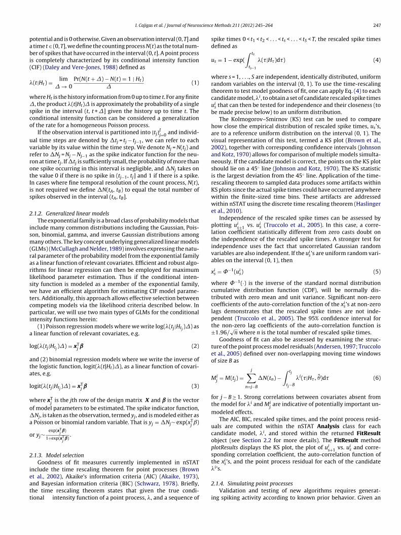
3. Code reuse: due to inheritance, methods need not be imple-mented for each new object. This leads to organization ofmethods across classes and simplified code maintenance. Thisproperty also improves code testing and maintenance by yield-ing increased code clarity and readability. For example, considerthe computation of the time rescaling theorem. Suppose we havea collection of spike times, 0 < t1 < t2 < . . . < ts < . . . < tS < T, repre-sented as a vector called spikeTimes, and a conditional intensityfunction, �(t|Ht), represented as a SignalObj called lambda. Therescaled spike times, us, from the time rescaling theorem arecomputed by the following code:

%% Tim e Rescalin g Theore mt_s = spikeTime s(2:end ); % t_ 1,... , t_ St_sMinus1 = spikeTime s(1:en d−1); % 0,t_1,.. .,t_{ S−1}lambdaInt = lambda.integra l;% lambdaIn t(t ) = integra l fro m 0 to t of lambd a(t )z_s=lambdaInt.getValueA t(t_s ) − lambdaInt.getValueA t(t_sMinus1) ;u_s=1−ex p(z_s) ;

where the integral method of class SignalObj returns a SignalObjobject. Since lambdaInt is an object of class SignalObj it has a get-ValueAt method that can be used to obtain the value of the integralat each of the spike times in the vectors t s and t sMinus1.

250 I. Cajigas et al. / Journal of Neuroscience Methods 211 (2012) 245– 264

Load D ata

Trial

Analysis

FitResultFitResSumma ry

nspikeTrainnstCollCovariateCovCollEvent

& Covariates

Create Trials

Specify D ata Analysis

Run Analysis

% Load D ata spikeTimes = impo rtdata('spikeD ata.t xt');

% Perform Anal ysis results =Anal ysi s.Run Anal ysisFor AllNeu rons(t ria l,tcc,0);

% Specify how to analy ze d ata

tc{1}.setName( 'Consta nt Baseline');

% Create the t rial stru ctu re trial = Trial(spike Col l,covar Coll);

nst = nspikeTrain(spik eTimes); time = 0:(1/sampleRate):ns t.ma xTime; spikeColl = nst Coll(nst); baseline = Covariate(tim e,ones(length(time),1) ,'Baseline ','time ','s ','',{'\mu'}); covar Coll = CovColl({baseline});

Visuali ze Results % Vizuali ze Results h=results.plot Results;

Code

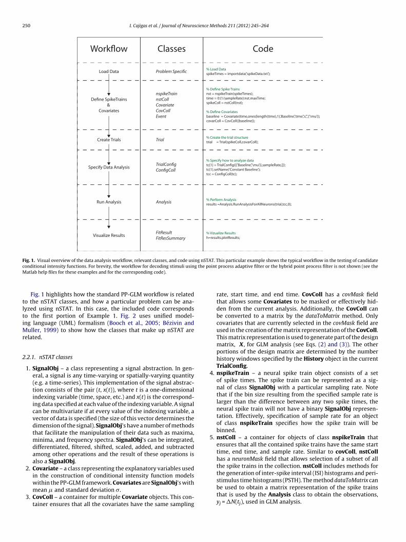
Fig. 1. Visual overview of the data analysis workflow, relevant classes, and code using nSTAT. This particular example shows the typical workflow in the testing of candidatec g the pM

tltiMr

2

onditional intensity functions. For brevity, the workflow for decoding stimuli usinatlab help files for these examples and for the corresponding code).

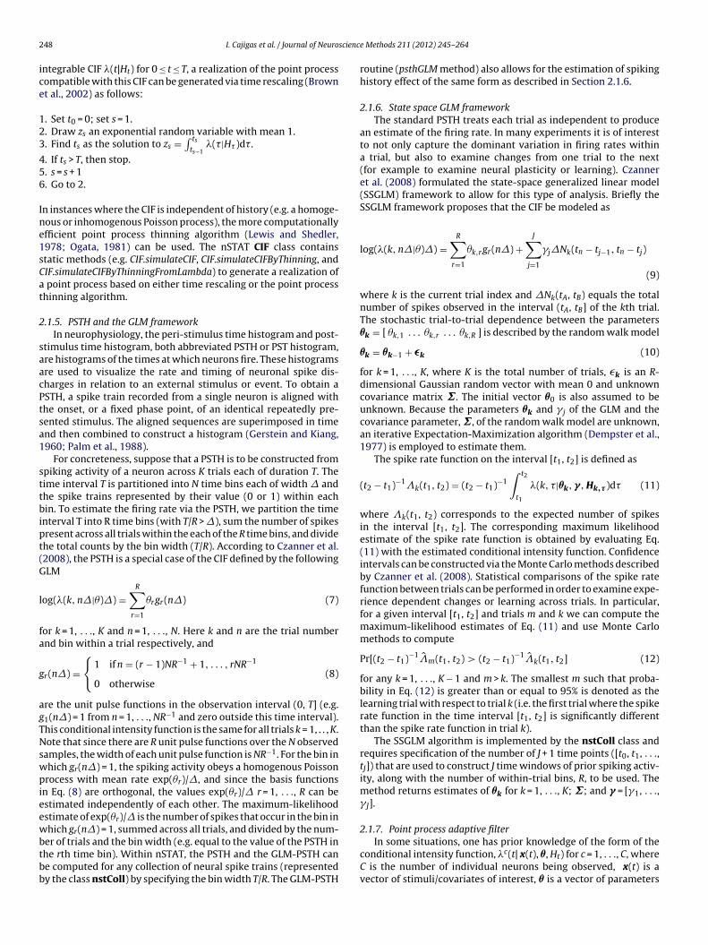
Fig. 1 highlights how the standard PP-GLM workflow is relatedo the nSTAT classes, and how a particular problem can be ana-yzed using nSTAT. In this case, the included code correspondso the first portion of Example 1. Fig. 2 uses unified model-ng language (UML) formalism (Booch et al., 2005; Bézivin and

uller, 1999) to show how the classes that make up nSTAT areelated.

.2.1. nSTAT classes

1. SignalObj – a class representing a signal abstraction. In gen-eral, a signal is any time-varying or spatially-varying quantity(e.g. a time-series). This implementation of the signal abstrac-tion consists of the pair (t, x(t)), where t is a one-dimensionalindexing variable (time, space, etc.) and x(t) is the correspond-ing data specified at each value of the indexing variable. A signalcan be multivariate if at every value of the indexing variable, avector of data is specified (the size of this vector determines thedimension of the signal). SignalObj’s have a number of methodsthat facilitate the manipulation of their data such as maxima,minima, and frequency spectra. SignalObj’s can be integrated,differentiated, filtered, shifted, scaled, added, and subtractedamong other operations and the result of these operations isalso a SignalObj.

2. Covariate – a class representing the explanatory variables usedin the construction of conditional intensity function models

within the PP-GLM framework. Covariates are SignalObj’s withmean � and standard deviation �.

3. CovColl – a container for multiple Covariate objects. This con-tainer ensures that all the covariates have the same sampling

oint process adaptive filter or the hybrid point process filter is not shown (see the

rate, start time, and end time. CovColl has a covMask fieldthat allows some Covariates to be masked or effectively hid-den from the current analysis. Additionally, the CovColl canbe converted to a matrix by the dataToMatrix method. Onlycovariates that are currently selected in the covMask field areused in the creation of the matrix representation of the CovColl.This matrix representation is used to generate part of the designmatrix, X , for GLM analysis (see Eqs. (2) and (3)). The otherportions of the design matrix are determined by the numberhistory windows specified by the History object in the currentTrialConfig.

4. nspikeTrain – a neural spike train object consists of a setof spike times. The spike train can be represented as a sig-nal of class SignalObj with a particular sampling rate. Notethat if the bin size resulting from the specified sample rate islarger than the difference between any two spike times, theneural spike train will not have a binary SignalObj represen-tation. Effectively, specification of sample rate for an objectof class nspikeTrain specifies how the spike train will bebinned.

5. nstColl – a container for objects of class nspikeTrain thatensures that all the contained spike trains have the same starttime, end time, and sample rate. Similar to covColl, nstCollhas a neuronMask field that allows selection of a subset of allthe spike trains in the collection. nstColl includes methods forthe generation of inter-spike interval (ISI) histograms and peri-

stimulus time histograms (PSTH). The method dataToMatrix canbe used to obtain a matrix representation of the spike trainsthat is used by the Analysis class to obtain the observations,yj = �N(tj), used in GLM analysis.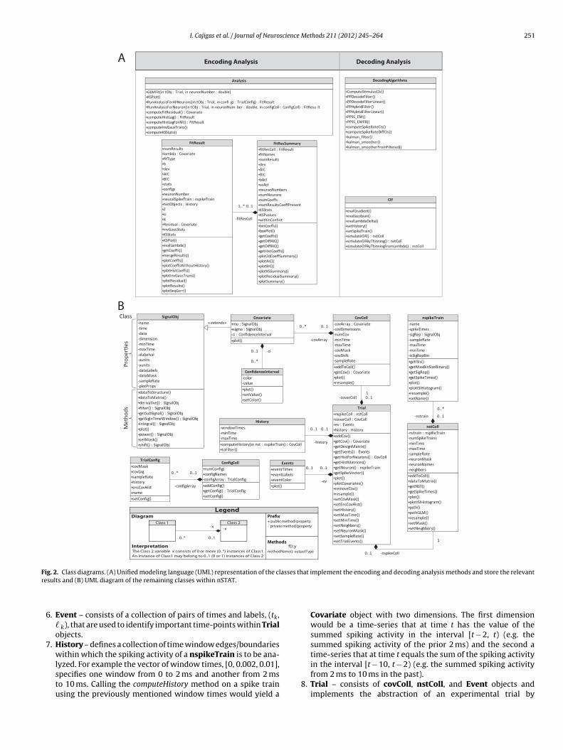

I. Cajigas et al. / Journal of Neuroscience Methods 211 (2012) 245– 264 251

Prop

er�e

s

Class

Met

hods

+add Cov()+getCov() : Covariate+getDesi gnMatrix()+getEvents() : Events+getHis tForNeurons() : CovColl+getHis tMatrices()+getNeuron() : nspikeTrain+getSpikeVector()+plot()+plotCovariates()+removeCov()+resample()+setCovMask()+setEnsCovHis t()+setHis tory()+setMaxTime()+setMinTime()+setNeighbors()+setNeuronMask()+setSampleRate()+setTrialEvents()

Tria l+nspikeColl : nstColl+covarColl : CovColl+ev : Events+his tory : His tory

+dataToStruc ture()+dataToMatrix()+deriva�ve() : SignalObj+filter() : SignalObj+getSubSignal() : SignalObj+getSigInTimeWindow() : SignalObj+integral() : SignalObj+plot()+pow er() : SignalObj+setMask()+shi�() : SignalObj

SignalObj-name-�me-data-dimensi on-minTime-maxTime-xlabelval-xunits-yunits-dataLabels-dataMask-sampleRate-plotProps

+plot()

Covaria te+mu : SignalObj+si gma : SignalObj-ci : ConfidenceInterval

+plot()

Events+eventTimes+eventLabels+eventColor

+computeHis tory(in nst : nspikeTrain) : CovColl+toFilter()

History-window Times-minTime-maxTime

+plot()+setValue()+setColor()

ConfidenceInterval-color-value

+add ToColl ()+getCov() : Covariate+plot()+resample()

CovColl-covArr ay : Covariate-covDimensi ons-numCov-minTime-maxTime-covMask-covShi�-sampleRate

+add ToColl ()+dataToMatrix()+getNST()+getSpikeTimes()+plot()+plotISIHis togram()+psth()+psthGLM()+resample()+setMask()+setNeighbors()

nstColl-nstrain : nspikeTrain-numSpikeTrains-minTime-maxTime-sampleRate-neuronMask-neuronNames-neighbors

+getISIs()+getMaxBinSizeBinary()+getSigRep()+getSpikeTimes()+plot()+plotISIHis togram()+resample()+setName()

nspik eTrai n-name-spikeTimes-si gRep : SignalObj-sampleRate-maxTime-minTime-is SigRepBin

«extends»

-nstrain 0.. 1

0.. *

-ev

0..10..1

-ci0.. 1

0.. *

+setConfig()

Tria lConfig+covMask+covLag+sampleRate+his tory+ensCovHis t+name

+add Config()+getConfig() : TrialConfig+setConfig()

ConfigColl+numConfigs+configNames-configArr ay : TrialConfig

-configArr ay

0..10.. *

-his tory

0.. 10.. 1

-nspikeColl0..1

1

-covArr ay

0.. 10.. *

-covarColl 0.. 11

-x -xClass 2Class 1

0..* 0..1

The Class 2 variable x consists of 0 or more (0..*) instances of Class1An instance of Class1 may belong to 0..1 (0 or 1) instances of Class 2

Diagram

Interpretation

Legend

+ public method/property- private method/property

methodName(): outputTypef():y

Methods

A

B

+GLMFit(in tObj : Trial, in neuronNumber : double)+KSPlot()+RunAnalysis ForAll Neurons(in tObj : Trial, in confi gs : TrialConfig) : FitResult+RunAnalysis ForNeuron(in tObj : Trial, in neuronNum ber : double, in configColl : ConfigColl ) : FitResu lt+computeFitResidual() : Covariate+computeHis tLag() : FitResult+computeHis tLagForAll() : FitResult+computeInv GausTrans()+computeKSS tats()

Analysis

+evalGradient()+evalJacobian()+evalLambdaDelta()+setHis tory()+setSpikeTrain()+si mulateCIF() : nstColl+si mulateCIFByThinn ing() : nstColl+si mulateCIFByThinn ingFromLambda() : nstColl

CIF

+ComputeS�mulusCIs()+PP DecodeFilter()+PP DecodeFilterLinea r()+PP HybridFilter()+PP HybridFilterLinear()+PPSS _EM()+PPSS _EMFB()+computeSpikeRateCIs()+computeSpikeRateDiffCIs()+kalman_filter()+kalman_smoo ther()+kalman_smoo therFromFiltered()

DecodingAlgorithms

-fitResCell

0.. 11.. *

+KSPlot()+evalLambda()+getCoeffs()+mergeResults()+plotCoeffs()+plotCoeffsWithoutHis tory()+plotHis tCoeffs()+plotInv GausTrans()+plotResi dual()+plotResults()+plotSeqCorr ()

FitRes ult+numResults+lambda : Covariate+fitType+b+dev+AIC+BIC+stats+configs+neuronNumber+neuralSpikeTrain : nspikeTrain+his tObje cts : His tory+Z+U+X+Residual : Covariate+inv GausStats+KSS tats

+binCoeffs()+boxPlot()+getCoeffs()+getDiffAIC()+getDiffBIC()+getHis tCoeffs()+plot2dCoeffSumm ary()+plotAIC()+plotBIC()+plotKSS umm ary()+plotResi dualSumm ary()+plotSumm ary()

FitResSu

u

mmary+fitResCell : FitResult+fitNames+numResults+dev+AIC+BIC+bAct+seAct+neuronNumbers+numNeurons+numCoeffs+numResultsCoeffPresent+KSS tats+KSPvalues+withinConfInt

Decoding AnalysisEncoding Analysis

Fig. 2. Class diagrams. (A) Unified modeling language (UML) representation of the classes that implement the encoding and decoding analysis methods and store the relevantr

esults and (B) UML diagram of the remaining classes within nSTAT.

6. Event – consists of a collection of pairs of times and labels, (tk, k), that are used to identify important time-points within Trialobjects.

7. History – defines a collection of time window edges/boundarieswithin which the spiking activity of a nspikeTrain is to be ana-

lyzed. For example the vector of window times, [0, 0.002, 0.01],specifies one window from 0 to 2 ms and another from 2 msto 10 ms. Calling the computeHistory method on a spike trainusing the previously mentioned window times would yield a

Covariate object with two dimensions. The first dimensionwould be a time-series that at time t has the value of thesummed spiking activity in the interval [t − 2, t) (e.g. thesummed spiking activity of the prior 2 ms) and the second atime-series that at time t equals the sum of the spiking activity

in the interval [t − 10, t − 2) (e.g. the summed spiking activityfrom 2 ms to 10 ms in the past).

8. Trial – consists of covColl, nstColl, and Event objects andimplements the abstraction of an experimental trial by

2 science Methods 211 (2012) 245– 264

11

1

1

1

1

2

2–

bo“sRodmst

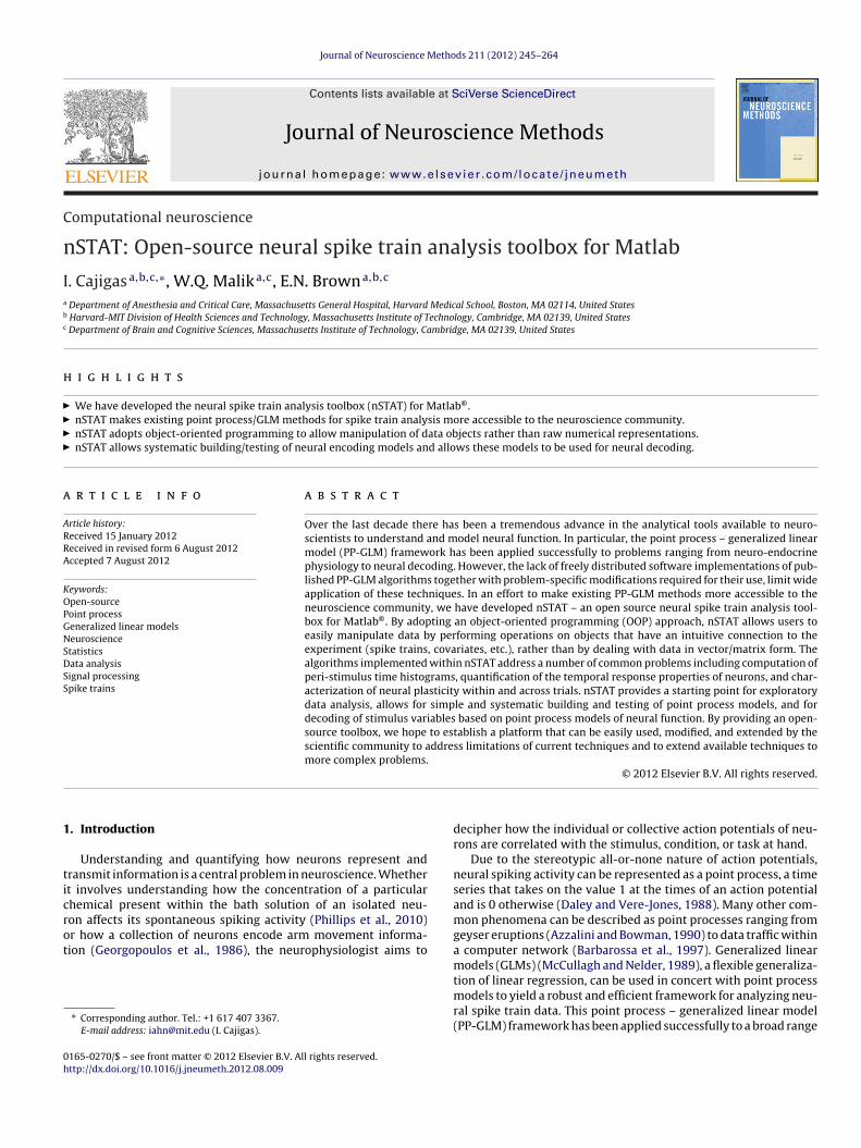
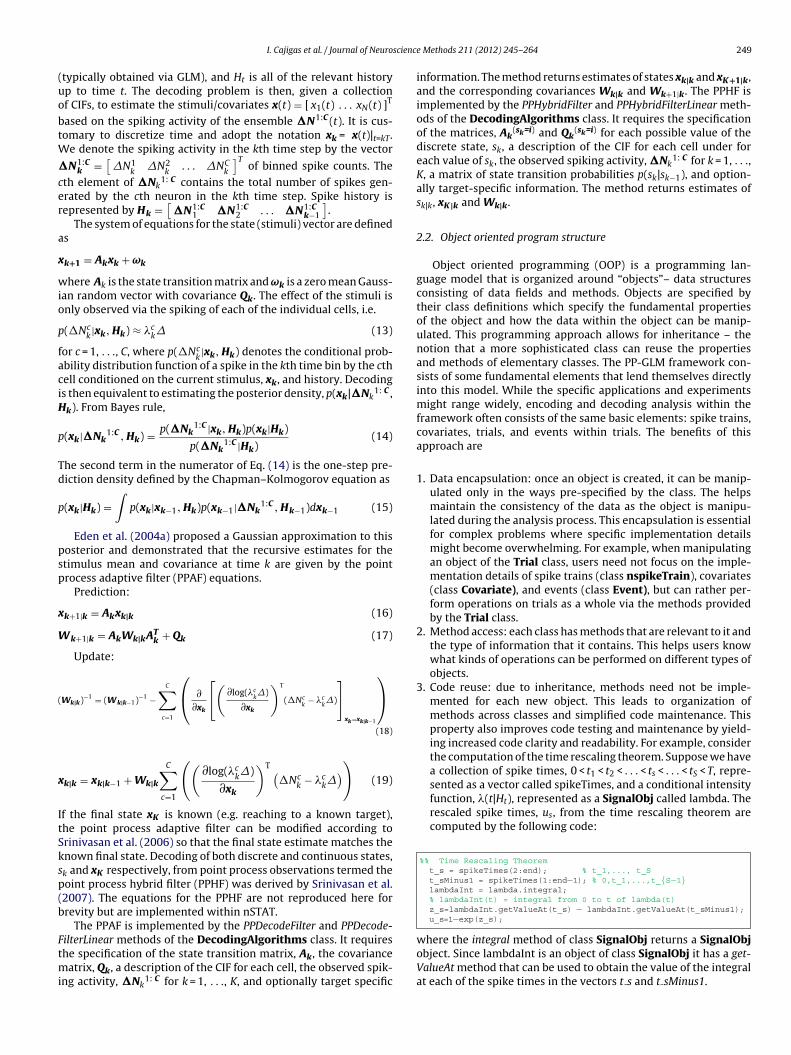
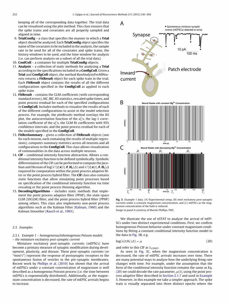
Fig. 3. Example 1 data. (A) Experimental setup, (B) mini excitatory post-synaptic

52 I. Cajigas et al. / Journal of Neuro

keeping all of the corresponding data together. The trial datacan be visualized using the plot method. This class ensures thatthe spike trains and covariates are all properly sampled andaligned in time.

9. TrialConfig – a class that specifies the manner in which a Trialobject should be analyzed. Each TrialConfig object specifies thename of the covariates to be included in the analysis, the samplerate to be used for all of the covariates and spike trains, thehistory windows to be used, and the time window for analysis(i.e. can perform analysis on a subset of all the trial data).

0. ConfColl – a container for multiple TrialConfig objects.1. Analysis – a collection of static methods for analyzing a Trial

according to the specifications included in a ConfigColl. Given aTrial and ConfigColl object, the method RunAnalysisForAllNeu-rons returns a FitResult object for each spike train in the trial.Each FitResult object contains the results of all the differentconfigurations specified in the ConfigColl as applied to eachspike train.

2. FitResult – contains the GLM coefficients (with correspondingstandard errors), AIC, BIC, KS statistics, rescaled spike times, andpoint process residual for each of the specified configurationsin ConfigColl. Includes methods to visualize the results of eachof the different configurations to assist in the model selectionprocess. For example, the plotResults method overlays the KSplot, the autocorrelation function of the ui

s’s, the lag-1 corre-lation coefficient of the ui

s’s, the GLM fit coefficients with 95%confidence intervals, and the point process residual for each ofthe models specified in the ConfigColl.

3. FitResSummary – given a collection of FitResult objects (onefor each neuron, each containing the results of multiple regres-sions), computes summary statistics across all neurons and allconfigurations in the ConfigColl. This class allows visualizationof commonalities in the data across multiple neurons.

4. CIF – conditional intensity function abstraction. Allows a con-ditional intensity function to be defined symbolically. Symbolicdifferentiation of the CIF can be performed to compute the Jaco-bian and Hessian of log(�c(t| x(t), �, Ht)�) and �c(t| x(t), �, Ht)�required for computation within the point process adaptive fil-ter or the point process hybrid filter. The CIF class also containsstatic functions that allow simulating point processes basedon specification of the conditional intensity function via timerescaling or the point process thinning algorithm.

5. DecodingAlgorithms – includes static methods that imple-ment the point process adaptive filter (PPAF), the state-spaceGLM (SSGLM) filter, and the point process hybrid filter (PPHF)among others. This class also implements non-point processalgorithms such as the Kalman Filter (Kalman, 1960) and theKalman Smoother (Rauch et al., 1965).

.3. Examples

.3.1. Example 1 – homogeneous/inhomogenous Poisson models the miniature excitatory post-synaptic current

Miniature excitatory post-synaptic currents (mEPSCs) haveecome a primary measure of synaptic modification during devel-pment, plasticity, and disease. These post-synaptic currents (ormini’s”) represent the response of postsynaptic receptors to thepontaneous fusion of vesicles in the pre-synaptic membranes.ecent work by Phillips et al. (2010) has shown that the arrivalf mEPSCs under a constant concentration of magnesium is well

escribed as a homogenous Poisson process (i.e. the time betweenEPSCs is exponentially distributed). Additionally, as the magne-

ium concentration is decreased, the rate of mEPSC arrivals beginso increase.

currents under a constant magnesium concentration, and (C) mEPSCs as the mag-nesium concentration of the bath is reduced.

Image in panel A courtesy of Marnie Phillips, PhD.

We illustrate the use of nSTAT to analyze the arrival of mEP-SCs under two distinct experimental conditions. First, we confirmhomogeneous Poisson behavior under constant magnesium condi-tions by fitting a constant conditional intensity function model tothe data in Fig. 3B, e.g.

log(�(t|Ht)�) = � (20)

and refer to this CIF as �CONST.As seen in Fig. 3C, when the magnesium concentration is

decreased, the rate of mEPSC arrivals increases over time. Thereare many potential ways to analyze how the underlying firing ratechanges with time. For example, under the assumption that theform of the conditional intensity function remains the same as Eq.

(20) we could decode the rate parameter, �(t), using the point pro-cess adaptive filter described in Section 2.1.7 and used in Example5. However, in this example we take a simpler approach. The spiketrain is visually separated into three distinct epochs where the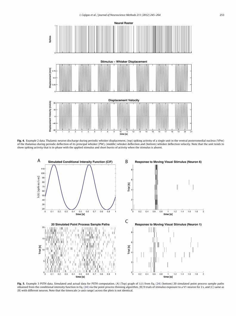

I. Cajigas et al. / Journal of Neuroscience Methods 211 (2012) 245– 264 253

Fig. 4. Example 2 data. Thalamic neuron discharge during periodic whisker displacement, (top) spiking activity of a single unit in the ventral posteromedial nucleus (VPm)of the thalamus during periodic deflection of its principal whisker (PW), (middle) whisker deflection and (bottom) whisker deflection velocity. Note that the unit tends toshow spiking activity that is in-phase with the applied stimulus and short bursts of activity when the stimulus is absent.

Fig. 5. Example 3 PSTH data. Simulated and actual data for PSTH computation. (A) (Top) graph of �(t) from Eq. (24) (bottom) 20 simulated point process sample pathsobtained from the conditional intensity function in Eq. (24) via the point process thinning algorithm, (B) 9 trials of stimulus exposure to a V1 neuron for 2 s, and (C) same as(B) with different neuron. Note that the timescale (x-axis range) across the plots is not identical.

254 I. Cajigas et al. / Journal of Neuroscience Methods 211 (2012) 245– 264

F ulusa thm df

b(s

l

Wto

2e

tspaewfnit1

torsm

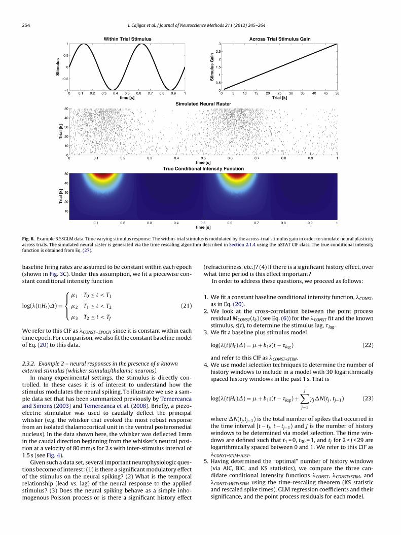
ig. 6. Example 3 SSGLM data. Time varying stimulus response. The within-trial stimcross trials. The simulated neural raster is generated via the time rescaling algoriunction is obtained from Eq. (27).

aseline firing rates are assumed to be constant within each epochshown in Fig. 3C). Under this assumption, we fit a piecewise con-tant conditional intensity function

og(�(t|Ht)�) =

⎧⎪⎨⎪⎩

�1 T0 ≤ t < T1

�2 T1 ≤ t < T2

�3 T2 ≤ t < Tf

(21)

e refer to this CIF as �CONST−EPOCH since it is constant within eachime epoch. For comparison, we also fit the constant baseline modelf Eq. (20) to this data.

.3.2. Example 2 – neural responses in the presence of a knownxternal stimulus (whisker stimulus/thalamic neurons)

In many experimental settings, the stimulus is directly con-rolled. In these cases it is of interest to understand how thetimulus modulates the neural spiking. To illustrate we use a sam-le data set that has been summarized previously by Temereancand Simons (2003) and Temereanca et al. (2008). Briefly, a piezo-lectric stimulator was used to caudally deflect the principalhisker (e.g. the whisker that evoked the most robust response

rom an isolated thalamocortical unit in the ventral posteromedialucleus). In the data shown here, the whisker was deflected 1mm

n the caudal direction beginning from the whisker’s neutral posi-ion at a velocity of 80 mm/s for 2 s with inter-stimulus interval of.5 s (see Fig. 4).

Given such a data set, several important neurophysiologic ques-ions become of interest: (1) is there a significant modulatory effect

f the stimulus on the neural spiking? (2) What is the temporalelationship (lead vs. lag) of the neural response to the appliedtimulus? (3) Does the neural spiking behave as a simple inho-ogenous Poisson process or is there a significant history effect

is modulated by the across-trial stimulus gain in order to simulate neural plasticityescribed in Section 2.1.4 using the nSTAT CIF class. The true conditional intensity

(refractoriness, etc.)? (4) If there is a significant history effect, overwhat time period is this effect important?

In order to address these questions, we proceed as follows:

1. We fit a constant baseline conditional intensity function, �CONST,as in Eq. (20).

2. We look at the cross-correlation between the point processresidual MCONST(tk) (see Eq. (6)) for the �CONST fit and the knownstimulus, s(t), to determine the stimulus lag, � lag.

3. We fit a baseline plus stimulus model

log(�(t|Ht)�) = � + b1s(t − �lag) (22)

and refer to this CIF as �CONST+STIM.4. We use model selection techniques to determine the number of

history windows to include in a model with 30 logarithmicallyspaced history windows in the past 1 s. That is

log(�(t|Ht)�) = � + b1s(t − �lag) +J∑

j=1

�j�N(tj, tj−1) (23)

where �N(tj,tj−1) is the total number of spikes that occurred inthe time interval [t − tj, t − tj−1) and J is the number of historywindows to be determined via model selection. The time win-dows are defined such that t1 = 0, t30 = 1, and tj for 2 < j < 29 arelogarithmically spaced between 0 and 1. We refer to this CIF as�CONST+STIM+HIST.

5. Having determined the “optimal” number of history windows(via AIC, BIC, and KS statistics), we compare the three can-

didate conditional intensity functions �CONST, �CONST+STIM, and�CONST+HIST+STIM using the time-rescaling theorem (KS statisticand rescaled spike times), GLM regression coefficients and theirsignificance, and the point process residuals for each model.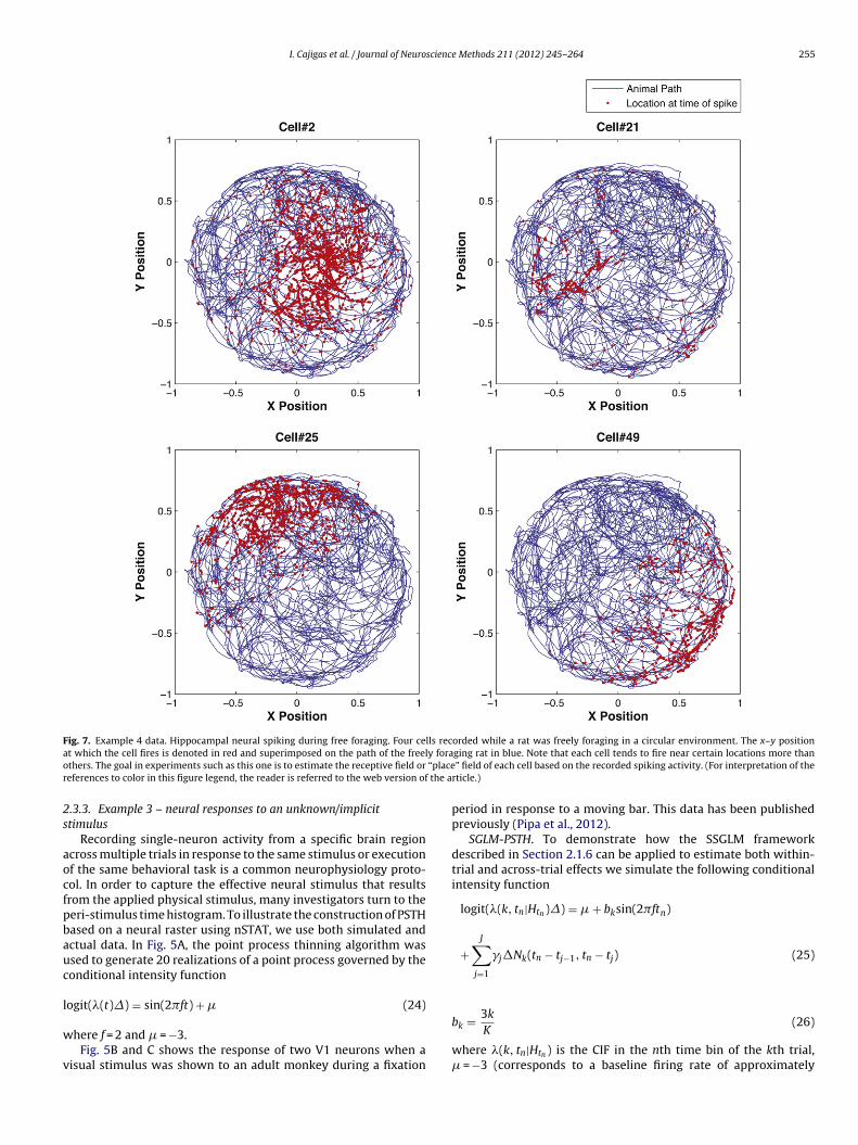

I. Cajigas et al. / Journal of Neuroscience Methods 211 (2012) 245– 264 255

Fig. 7. Example 4 data. Hippocampal neural spiking during free foraging. Four cells recorded while a rat was freely foraging in a circular environment. The x–y positiona y forao “placer the a

2s

aocfpbauc

l

w

v

t which the cell fires is denoted in red and superimposed on the path of the freelthers. The goal in experiments such as this one is to estimate the receptive field oreferences to color in this figure legend, the reader is referred to the web version of

.3.3. Example 3 – neural responses to an unknown/implicittimulus

Recording single-neuron activity from a specific brain regioncross multiple trials in response to the same stimulus or executionf the same behavioral task is a common neurophysiology proto-ol. In order to capture the effective neural stimulus that resultsrom the applied physical stimulus, many investigators turn to theeri-stimulus time histogram. To illustrate the construction of PSTHased on a neural raster using nSTAT, we use both simulated andctual data. In Fig. 5A, the point process thinning algorithm wassed to generate 20 realizations of a point process governed by theonditional intensity function

ogit(�(t)�) = sin(2�ft) + � (24)

here f = 2 and � = −3.Fig. 5B and C shows the response of two V1 neurons when a

isual stimulus was shown to an adult monkey during a fixation

ging rat in blue. Note that each cell tends to fire near certain locations more than” field of each cell based on the recorded spiking activity. (For interpretation of the

rticle.)

period in response to a moving bar. This data has been publishedpreviously (Pipa et al., 2012).

SGLM-PSTH. To demonstrate how the SSGLM frameworkdescribed in Section 2.1.6 can be applied to estimate both within-trial and across-trial effects we simulate the following conditionalintensity function

logit(�(k, tn|Htn )�) = � + bksin(2�ftn)

+J∑

j=1

�j�Nk(tn − tj−1, tn − tj) (25)

bk = 3k

K(26)

where �(k, tn|Htn ) is the CIF in the nth time bin of the kth trial,� = −3 (corresponds to a baseline firing rate of approximately

256 I. Cajigas et al. / Journal of Neuroscience Methods 211 (2012) 245– 264

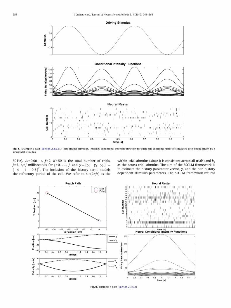
F nal ints

5J

[t

ig. 8. Example 5 data (Section 2.3.5.1). (Top) driving stimulus, (middle) conditioinusoidal stimulus.

0 Hz), � = 0.001 s, f = 2, K = 50 is the total number of trials,

= 3, tj = j milliseconds for j = 0, . . ., J, and � = [ �1 �2 �3 ]T =−4 −1 −0.5 ]T . The inclusion of the history term modelshe refractory period of the cell. We refer to sin(2�ft) as the

Fig. 9. Example 5 data

ensity function for each cell, (bottom) raster of simulated cells begin driven by a

within-trial stimulus (since it is consistent across all trials) and b

kas the across-trial stimulus. The aim of the SSGLM framework isto estimate the history parameter vector, � , and the non-historydependent stimulus parameters. The SSGLM framework returns

(Section 2.3.5.2).

I. Cajigas et al. / Journal of Neuroscience Methods 211 (2012) 245– 264 257

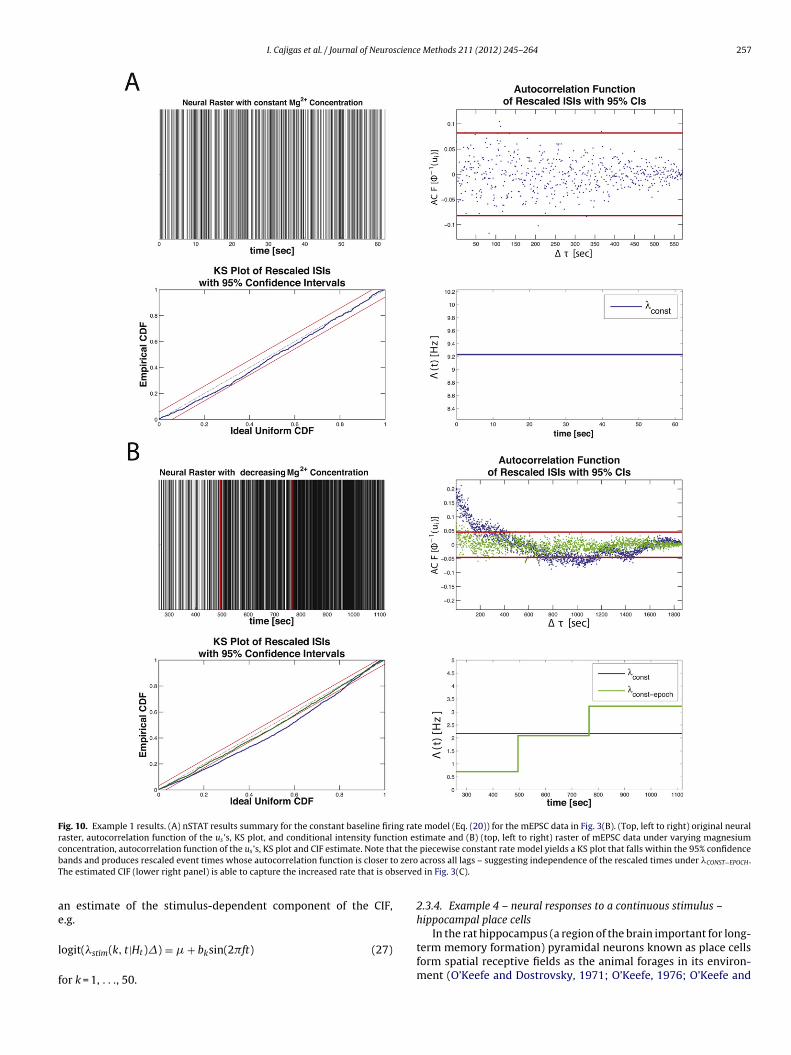
Fig. 10. Example 1 results. (A) nSTAT results summary for the constant baseline firing rate model (Eq. (20)) for the mEPSC data in Fig. 3(B). (Top, left to right) original neuralraster, autocorrelation function of the us ’s, KS plot, and conditional intensity function estimate and (B) (top, left to right) raster of mEPSC data under varying magnesiumc at theb o zeroT serve

ae

l

f

oncentration, autocorrelation function of the us ’s, KS plot and CIF estimate. Note thands and produces rescaled event times whose autocorrelation function is closer the estimated CIF (lower right panel) is able to capture the increased rate that is ob

n estimate of the stimulus-dependent component of the CIF,.g.

ogit(�stim(k, t|Ht)�) = � + bksin(2�ft) (27)

or k = 1, . . ., 50.

piecewise constant rate model yields a KS plot that falls within the 95% confidence across all lags – suggesting independence of the rescaled times under �CONST−EPOCH .d in Fig. 3(C).

2.3.4. Example 4 – neural responses to a continuous stimulus –hippocampal place cells

In the rat hippocampus (a region of the brain important for long-term memory formation) pyramidal neurons known as place cellsform spatial receptive fields as the animal forages in its environ-ment (O’Keefe and Dostrovsky, 1971; O’Keefe, 1976; O’Keefe and

258 I. Cajigas et al. / Journal of Neuroscience Methods 211 (2012) 245– 264

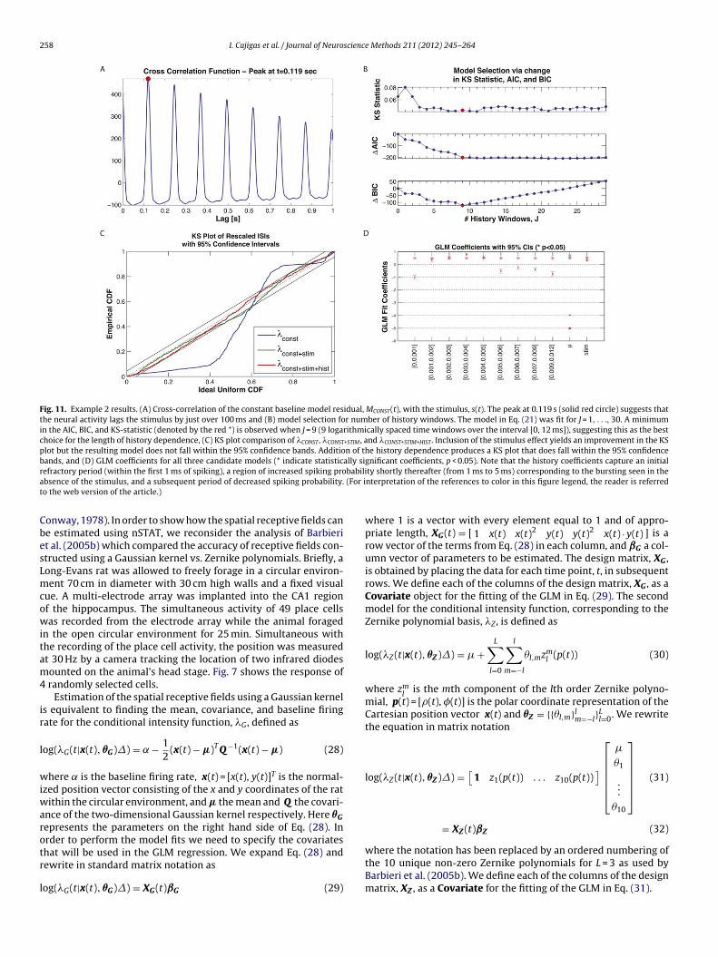
Fig. 11. Example 2 results. (A) Cross-correlation of the constant baseline model residual, MCONST(t), with the stimulus, s(t). The peak at 0.119 s (solid red circle) suggests thatthe neural activity lags the stimulus by just over 100 ms and (B) model selection for number of history windows. The model in Eq. (21) was fit for J = 1, . . ., 30. A minimumin the AIC, BIC, and KS-statistic (denoted by the red *) is observed when J = 9 (9 logarithmically spaced time windows over the interval [0, 12 ms]), suggesting this as the bestchoice for the length of history dependence, (C) KS plot comparison of �CONST , �CONST+STIM , and �CONST+STIM+HIST . Inclusion of the stimulus effect yields an improvement in the KSplot but the resulting model does not fall within the 95% confidence bands. Addition of the history dependence produces a KS plot that does fall within the 95% confidencebands, and (D) GLM coefficients for all three candidate models (* indicate statistically significant coefficients, p < 0.05). Note that the history coefficients capture an initialr babilia (For it

CbesLmcowitam4

ir

l

wiwarotr

l

efractory period (within the first 1 ms of spiking), a region of increased spiking probsence of the stimulus, and a subsequent period of decreased spiking probability.o the web version of the article.)

onway, 1978). In order to show how the spatial receptive fields cane estimated using nSTAT, we reconsider the analysis of Barbierit al. (2005b) which compared the accuracy of receptive fields con-tructed using a Gaussian kernel vs. Zernike polynomials. Briefly, aong-Evans rat was allowed to freely forage in a circular environ-ent 70 cm in diameter with 30 cm high walls and a fixed visual

ue. A multi-electrode array was implanted into the CA1 regionf the hippocampus. The simultaneous activity of 49 place cellsas recorded from the electrode array while the animal foraged

n the open circular environment for 25 min. Simultaneous withhe recording of the place cell activity, the position was measuredt 30 Hz by a camera tracking the location of two infrared diodesounted on the animal’s head stage. Fig. 7 shows the response of

randomly selected cells.Estimation of the spatial receptive fields using a Gaussian kernel

s equivalent to finding the mean, covariance, and baseline firingate for the conditional intensity function, �G, defined as

og(�G(t|x(t), �G)�) = ̨ − 12

(x(t) − �)T Q −1(x(t) − �) (28)

here ̨ is the baseline firing rate, x(t) = [x(t), y(t)]T is the normal-zed position vector consisting of the x and y coordinates of the rat

ithin the circular environment, and � the mean and Q the covari-nce of the two-dimensional Gaussian kernel respectively. Here �G

epresents the parameters on the right hand side of Eq. (28). Inrder to perform the model fits we need to specify the covariates

hat will be used in the GLM regression. We expand Eq. (28) andewrite in standard matrix notation as

og(�G(t|x(t), �G)�) = XG(t)ˇG (29)

ty shortly thereafter (from 1 ms to 5 ms) corresponding to the bursting seen in thenterpretation of the references to color in this figure legend, the reader is referred

where 1 is a vector with every element equal to 1 and of appro-priate length, XG(t) = [ 1 x(t) x(t)2 y(t) y(t)2 x(t) · y(t) ] is arow vector of the terms from Eq. (28) in each column, and ˇG a col-umn vector of parameters to be estimated. The design matrix, XG ,is obtained by placing the data for each time point, t, in subsequentrows. We define each of the columns of the design matrix, XG , as aCovariate object for the fitting of the GLM in Eq. (29). The secondmodel for the conditional intensity function, corresponding to theZernike polynomial basis, �Z, is defined as

log(�Z (t|x(t), �Z)�) = � +L∑

l=0

l∑m=−l

�l,mzml (p(t)) (30)

where zml

is the mth component of the lth order Zernike polyno-mial, p(t) = [�(t), �(t)] is the polar coordinate representation of theCartesian position vector x(t) and �Z = {{�l,m}l

m=−l}Ll=0. We rewrite

the equation in matrix notation

log(�Z (t|x(t), �Z)�) =[

1 z1(p(t)) . . . z10(p(t))]⎡⎢⎢⎢⎢⎣

�

�1

...

�10

⎤⎥⎥⎥⎥⎦ (31)

= XZ(t)ˇZ (32)

where the notation has been replaced by an ordered numbering ofthe 10 unique non-zero Zernike polynomials for L = 3 as used byBarbieri et al. (2005b). We define each of the columns of the designmatrix, XZ , as a Covariate for the fitting of the GLM in Eq. (31).

I. Cajigas et al. / Journal of Neuroscience Methods 211 (2012) 245– 264 259

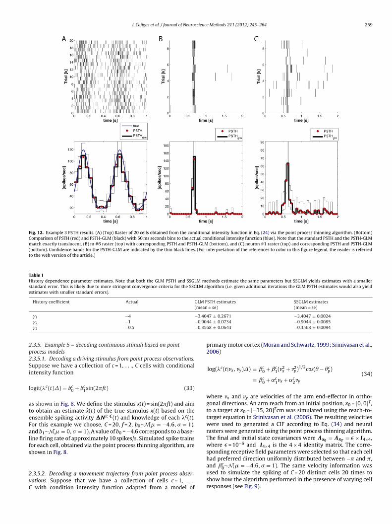
Fig. 12. Example 3 PSTH results. (A) (Top) Raster of 20 cells obtained from the conditional intensity function in Eq. (24) via the point process thinning algorithm. (Bottom)Comparison of PSTH (red) and PSTH-GLM (black) with 50 ms seconds bins to the actual conditional intensity function (blue). Note that the standard PSTH and the PSTH-GLMmatch exactly translucent. (B) m #6 raster (top) with corresponding PSTH and PSTH-GLM (bottom), and (C) neuron #1 raster (top) and corresponding PSTH and PSTH-GLM(bottom). Confidence bands for the PSTH-GLM are indicated by the thin black lines. (For interpretation of the references to color in this figure legend, the reader is referredto the web version of the article.)

Table 1History dependence parameter estimates. Note that both the GLM PSTH and SSGLM methods estimate the same parameters but SSGLM yields estimates with a smallerstandard error. This is likely due to more stringent convergence criteria for the SSGLM algorithm (i.e. given additional iterations the GLM PSTH estimates would also yieldestimates with smaller standard errors).

History coefficient Actual GLM PSTH estimates(mean ± se)

SSGLM estimates(mean ± se)

−3.40−0.90−0.35

2p2Si

l

ateFalfs

2vC

�1 −4

�2 −1

�2 −0.5

.3.5. Example 5 – decoding continuous stimuli based on pointrocess models.3.5.1. Decoding a driving stimulus from point process observations.uppose we have a collection of c = 1, . . ., C cells with conditionalntensity function

ogit(�c(t)�) = bc0 + bc

1sin(2�ft) (33)

s shown in Fig. 8. We define the stimulus x(t) = sin(2�ft) and aimo obtain an estimate x̂(t) of the true stimulus x(t) based on thensemble spiking activity �N1: C (t) and knowledge of each �c(t).or this example we choose, C = 20, f = 2, b0∼N(� = −4.6, � = 1),nd b1∼N(� = 0, � = 1). A value of b0 = −4.6 corresponds to a base-ine firing rate of approximately 10 spikes/s. Simulated spike trainsor each cell, obtained via the point process thinning algorithm, arehown in Fig. 8.

.3.5.2. Decoding a movement trajectory from point process obser-ations. Suppose that we have a collection of cells c = 1, . . .,

with condition intensity function adapted from a model of

47 ± 0.2671 −3.4047 ± 0.002444 ± 0.0734 −0.9044 ± 0.008568 ± 0.0643 −0.3568 ± 0.0094

primary motor cortex (Moran and Schwartz, 1999; Srinivasan et al.,2006)

log(�c(t|vx, vy)�) = ˇc0 + ˇc

1(v2x + v2

y)1/2cos(� − �cp)

= ˇc0 + ˛c

1vx + ˛c2vy

(34)

where vx and vy are velocities of the arm end-effector in ortho-gonal directions. An arm reach from an initial position, x0 = [0, 0]T,to a target at x0 = [−35, 20]Tcm was simulated using the reach-to-target equation in Srinivasan et al. (2006). The resulting velocitieswere used to generated a CIF according to Eq. (34) and neuralrasters were generated using the point process thinning algorithm.The final and initial state covariances were x0 = xT = � × I4×4,where � = 10−6 and I4×4 is the 4 × 4 identity matrix. The corre-sponding receptive field parameters were selected so that each cellhad preferred direction uniformly distributed between −� and �,

and ˇc

0∼N(� = −4.6, � = 1). The same velocity information wasused to simulate the spiking of C = 20 distinct cells 20 times toshow how the algorithm performed in the presence of varying cellresponses (see Fig. 9).

260 I. Cajigas et al. / Journal of Neuroscience Methods 211 (2012) 245– 264

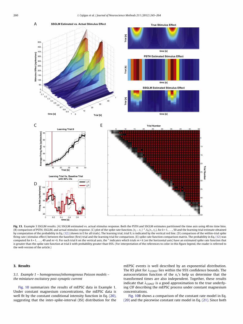
Fig. 13. Example 3 SSGLM results. (A) SSGLM estimated vs. actual stimulus response. Both the PSTH and SSGLM estimates partitioned the time axis using 40 ms time bins.(B) comparison of PSTH, SSGLM, and actual stimulus response. (C) plot of the spike rate function, (t2 − t1)−1k(t1, t2), for k = 1, . . ., 50 and the learning trial estimate obtainedby computation of the probability in Eq. (12) (shown in E for all trials). The learning trial, trial 9, is indicated by the vertical red line. (D) comparison of the within-trial spikefiring rate (stimulus effect) between the baseline (first) trial and the learning trial for comparison. (E) spike rate function comparison matrix. The probability in Eq. (12) wascomputed for k = 1, . . ., 49 and m > k. For each trial k on the vertical axis, the * indicates which trials m > k (on the horizontal axis) have an estimated spike rate function thatis greater than the spike rate function at trial k with probability greater than 95%. (For interpretation of the references to color in this figure legend, the reader is referred tothe web version of the article.)

3

3t

Uws

. Results

.1. Example 1 – homogeneous/inhomogenous Poisson models –he miniature excitatory post-synaptic current

Fig. 10 summarizes the results of mEPSC data in Example 1.nder constant magnesium concentrations, the mEPSC data isell fit by the constant conditional intensity function in Eq. (20),

uggesting that the inter-spike-interval (ISI) distribution for the

mEPSC events is well described by an exponential distribution.The KS plot for �CONST lies within the 95% confidence bounds. Theautocorrelation function of the xs’s help us determine that thetransformed times are also independent. Together, these resultsindicate that �CONST is a good approximation to the true underly-

ing CIF describing the mEPSC process under constant magnesiumconcentrations.

Fig. 10B shows a comparison of the constant rate model in Eq.(20) and the piecewise constant rate model in Eq. (21). Since both

I. Cajigas et al. / Journal of Neuroscience Methods 211 (2012) 245– 264 261

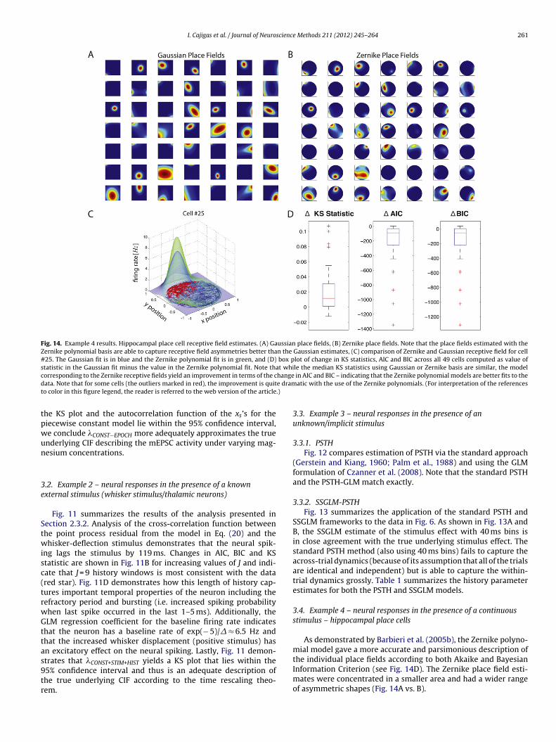
Fig. 14. Example 4 results. Hippocampal place cell receptive field estimates. (A) Gaussian place fields, (B) Zernike place fields. Note that the place fields estimated with theZernike polynomial basis are able to capture receptive field asymmetries better than the Gaussian estimates, (C) comparison of Zernike and Gaussian receptive field for cell#25. The Gaussian fit is in blue and the Zernike polynomial fit is in green, and (D) box plot of change in KS statistics, AIC and BIC across all 49 cells computed as value ofstatistic in the Gaussian fit minus the value in the Zernike polynomial fit. Note that while the median KS statistics using Gaussian or Zernike basis are similar, the modelc hanged e dramt .)

tpwun

3e

Stwisc(trwGttas9tr

orresponding to the Zernike receptive fields yield an improvement in terms of the cata. Note that for some cells (the outliers marked in red), the improvement is quito color in this figure legend, the reader is referred to the web version of the article

he KS plot and the autocorrelation function of the xs’s for theiecewise constant model lie within the 95% confidence interval,e conclude �CONST−EPOCH more adequately approximates the truenderlying CIF describing the mEPSC activity under varying mag-esium concentrations.

.2. Example 2 – neural responses in the presence of a knownxternal stimulus (whisker stimulus/thalamic neurons)

Fig. 11 summarizes the results of the analysis presented inection 2.3.2. Analysis of the cross-correlation function betweenhe point process residual from the model in Eq. (20) and thehisker-deflection stimulus demonstrates that the neural spik-

ng lags the stimulus by 119 ms. Changes in AIC, BIC and KStatistic are shown in Fig. 11B for increasing values of J and indi-ate that J = 9 history windows is most consistent with the datared star). Fig. 11D demonstrates how this length of history cap-ures important temporal properties of the neuron including theefractory period and bursting (i.e. increased spiking probabilityhen last spike occurred in the last 1–5 ms). Additionally, theLM regression coefficient for the baseline firing rate indicates

hat the neuron has a baseline rate of exp(− 5)/� ≈ 6.5 Hz andhat the increased whisker displacement (positive stimulus) hasn excitatory effect on the neural spiking. Lastly, Fig. 11 demon-

trates that �CONST+STIM+HIST yields a KS plot that lies within the5% confidence interval and thus is an adequate description ofhe true underlying CIF according to the time rescaling theo-em.

in AIC and BIC – indicating that the Zernike polynomial models are better fits to theatic with the use of the Zernike polynomials. (For interpretation of the references

3.3. Example 3 – neural responses in the presence of anunknown/implicit stimulus

3.3.1. PSTHFig. 12 compares estimation of PSTH via the standard approach

(Gerstein and Kiang, 1960; Palm et al., 1988) and using the GLMformulation of Czanner et al. (2008). Note that the standard PSTHand the PSTH-GLM match exactly.

3.3.2. SSGLM-PSTHFig. 13 summarizes the application of the standard PSTH and

SSGLM frameworks to the data in Fig. 6. As shown in Fig. 13A andB, the SSGLM estimate of the stimulus effect with 40 ms bins isin close agreement with the true underlying stimulus effect. Thestandard PSTH method (also using 40 ms bins) fails to capture theacross-trial dynamics (because of its assumption that all of the trialsare identical and independent) but is able to capture the within-trial dynamics grossly. Table 1 summarizes the history parameterestimates for both the PSTH and SSGLM models.

3.4. Example 4 – neural responses in the presence of a continuousstimulus – hippocampal place cells

As demonstrated by Barbieri et al. (2005b), the Zernike polyno-mial model gave a more accurate and parsimonious description of

the individual place fields according to both Akaike and BayesianInformation Criterion (see Fig. 14D). The Zernike place field esti-mates were concentrated in a smaller area and had a wider rangeof asymmetric shapes (Fig. 14A vs. B).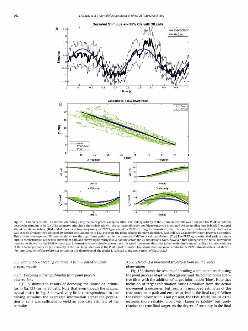

262 I. Cajigas et al. / Journal of Neuroscience Methods 211 (2012) 245– 264

Fig. 15. Example 5 results. (A) Stimulus decoding using the point process adaptive filter. The spiking activity of the 20 simulated cells was used with the PPAF in order todecode the stimulus in Eq. (24). The estimated stimulus is shown in black with the corresponding 95% confidence intervals illustrated by surrounding lines in black. The actualstimulus is shown in blue. (B) decoded movement trajectory using the PPAF (green) and the PPAF with target information (blue). For each trace, the true velocity informationwas used to simulate the spiking of 20 distinct cells according to Eq. (34) using the point process thinning algorithm. Each cell had a randomly chosen preferred direction.This process was repeated 20 times to show how the algorithms performed in the presence of different cell populations. (Top) The PPAF +goal estimated path in a morefaithful reconstruction of the true movement path and shows significantly less variability across the 20 simulations. Note, however, that comparison the actual movementtrajectories shows that the PPAF without goal information is more closely able to track the actual movement dynamics (albeit with significant variability). As the covarianceo oal es( rred to

3p

3o

lndts

f the final target increases (i.e. certainty in the final target decreases), the PPAF +gFor interpretation of the references to color in this figure legend, the reader is refe

.5. Example 5 – decoding continuous stimuli based on pointrocess models

.5.1. Decoding a driving stimulus from point processbservations

Fig. 15 shows the results of decoding the sinusoidal stimu-us in Eq. (33) using 20 cells. Note that even though the original

eural raster in Fig. 8 showed very little correspondence to theriving stimulus, the aggregate information across the popula-ion of cells was sufficient to yield an adequate estimate of thetimulus.

timated trajectories become more similar to the PPAF estimates (data not shown). the web version of the article.)

3.5.2. Decoding a movement trajectory from point processobservations

Fig. 15B shows the results of decoding a simulated reach usingthe point process adaptive filter (green) and the point process adap-tive filter with the addition of target information (blue). Note thatinclusion of target information causes deviation from the actualmovement trajectories, but results in improved estimates of the

true movement path and ensures arrival at the final target. Whenthe target information is not present, the PPAF tracks the true tra-jectories more reliably (albeit with larger variability) but rarelyreaches the true final target. As the degree of certainty in the final

scienc

tdP

4

(gntebinntaoie

t(z((tdeiea

ufpsaemmmum2tRo2

A

aISLIttmR

I. Cajigas et al. / Journal of Neuro

arget is decreased (i.e. the final target covariance increases), theecoded trajectories become increasingly similar to the standardPAF without target information.

. Discussion

We have developed the neural spike train analysis toolboxnSTAT) for Matlab® to facilitate the use of the point process –eneralized linear model framework by the neuroscience commu-ity. By providing a simple software interface to PP-GLM specificechniques within the Matlab® environment, users of a number ofxisting open source toolboxes (i.e. Chronux, STAToolkit, etc.) wille able to easily integrate these techniques into their workflow. It

s our hope that making nSTAT available in an open-source man-er will shorten the gap between innovation in the development ofew data analytic techniques and their practical application withinhe scientific community. For the neurophysiologist, we hope thevailability of such a tool will allow them to quickly test the rangef available methods with their data and use the results to bothnform the quality of their data and refine the protocols of theirxperiments.

Via a series of examples we have demonstrated the use of theoolbox to solve many common neuroscience problems including:1) systematic building of models of neural spiking, (2) characteri-ation of explicit experimental stimulus effects on neural spiking,3) spike rate estimation using the PSTH and extensions of the PSTHSSGLM) that allow quantification of experience-dependent plas-icity (across-trial effects), (4) receptive field estimation, and (5)ecoding stimuli such as movement trajectories based on mod-ls of neural firing. All of the data, code, and figures used here arencluded as part of the toolbox. We hope that users will be able toasily modify these examples and use them as a starting point fornalysis of their own data.

While the current release of nSTAT contains many commonlysed algorithms for analysis of neural data within the PP-GLMramework, there are many avenues for future improvement. Inarticular, optimization of current algorithm implementations toupport the GPU- and parallel-computing methods within Matlab®

re likely to be important for dealing with large data sets. Wencourage users to identify areas were the software can be madeore efficient and to make their contributions available to the com-unity at large. Future work for nSTAT will include the addition ofethods to deal with simultaneous analysis of neural ensembles

sing multivariate point-process theory together with multino-ial generalized linear models (mGLMs) (Chen et al., 2009b; Ba,

011; Brown et al., 2004), network analysis of multivariate spikerains(Brown et al., 2004; Krumin and Shoham, 2010; Stam andeijneveld, 2007; Bullmore and Sporns, 2009), and incorporationf causal modeling techniques for neural ensembles (Kim et al.,011) among others.

cknowledgements

This work was supported by NIH F31NS058275 – “Automatednd Adaptive Lower Extremity Neuro-Rehabilitation for Stroke” toahn Cajigas. The authors are indebted to Riccardo Barbieri andimona Temereanca (Harvard Medical School), Marnie Phillips,aura Lewis, and Demba Ba (MIT), and Gordon Pipa (Max Plancknstitute for Brain Research) for providing the data used to make

he examples. The authors would like to thank the reviewers forheir constructive comments and suggestions for improving the

anuscript, and the members of the MIT Neuroscience Statisticsesearch Lab for their collegial support.

e Methods 211 (2012) 245– 264 263

References

Ahmadian Y, Pillow JW, Paninski LL. Efficient Markov chain Monte Carlo methodsfor decoding neural spike trains. Neural Comput 2011;23(1):46–96.

Akaike H. Information theory and an extension of the maximum likelihood princi-ple. In: Second international symposium on information theory, vol. 1; 1973. p.267–81.

Andersen PK. Statistical models based on counting processes. New York: Springer;1997.

Azzalini A, Bowman AW. A look at some data on the old faithful geyser. Appl Stat1990;39(3):357–65.

Ba DE. Algorithms and inference for simultaneous-event multivariate point-process,with applications to neural data. Ph.D. thesis. Cambridge: Massachusetts Insti-tute of Technology; 2011.

Barbarossa S, Scaglione A, Baiocchi A, Colletti G. Modeling network traffic data bydoubly stochastic point processes with self-similar intensity process and frac-tal renewal point process. In: Conference record of the thirty-first Asilomarconference on signals, systems & computers; 1997. p. 1112–6.

Barbieri R, Brown EN. A point process adaptive filter for time-variant analysis ofheart rate variability. In: IEMBS ’04. 26th annual international conference of theIEEE. Engineering in Medicine and Biology Society; 2004. p. 3941–4.

Barbieri R, Brown EN. Analysis of heartbeat dynamics by point process adaptivefiltering. IEEE Trans Biomed Eng 2006a;53(1):4–12.

Barbieri R, Brown EN. Correction of erroneous and ectopic beats using a point processadaptive algorithm. In: Conference proceedings: annual international confer-ence of the IEEE engineering in medicine and biology society IEEE engineeringin medicine and biology society conference, vol. 1; 2006b. p. 3373–6.

Barbieri R, Chen Z, Brown EN. Assessment of hippocampal and autonomic neuralactivity by point process models. In: Conference proceedings: annual interna-tional conference of the IEEE engineering in medicine and biology society. IEEEengineering in medicine and biology society conference; 2008. p. 3679.

Barbieri R, Frank LM, Nguyen DP, Quirk MC, Solo V, Wilson MA, et al. Dynamicanalyses of information encoding in neural ensembles. Neural Comput2004;16(2):277–307.

Barbieri R, Matten EC, Alabi AA, Brown EN. A point-process model of human heart-beat intervals: new definitions of heart rate and heart rate variability. Am JPhysiol Heart Circ Physiol 2005a;288(1):H424–35.

Barbieri R, Wilson MA, Frank LM, Brown EN. An analysis of hippocampal spatio-temporal representations using a Bayesian algorithm for neural spike traindecoding. IEEE Trans Neural Syst Rehabil Eng 2005b;13(2):131–6.

Bézivin J, Muller PA. The unified modeling language. In: UML ’98: beyond the nota-tion: first international workshop. Springer Verlag; 1999.

Boashash B. Estimating and interpreting the instantaneous frequency of a signal. I.Fundamentals. In: Proceedings of the IEEE; 1992. p. 520–38.

Bokil H, Andrews P, Kulkarni JE, Mehta S, Mitra PP. Chronux: a platform for analyzingneural signals. J Neurosci Methods 2010;192(1):146–51.

Booch G, Rumbaugh J, Jacobson I. The unified modeling language user guide.Addison-Wesley Professional; 2005.

Brown EN, Barbieri R, Ventura V, Kass RE, Frank LM. The time-rescaling theo-rem and its application to neural spike train data analysis. Neural Comput2002;14(2):325–46.

Brown EN, Kass RE, Mitra PP. Multiple neural spike train data analysis:state-of-the-art and future challenges. Nat Neurosci 2004;7(5):456–61.

Brown EN, Meehan PM, Dempster AP. A stochastic differential equation model ofdiurnal cortisol patterns. Am J Physiol Endocrinol Metab 2001;280(3):E450–61.

Bullmore E, Sporns O. Complex brain networks: graph theoretical analysis of struc-tural and functional systems. Nat Rev 2009;10(3):186–98.

Chen Z, Brown EN, Barbieri R. A point process approach to assess dynamic baroreflexgain. Comput Cardiol 2008a;35:805–8.

Chen Z, Brown EN, Barbieri R. A study of probabilistic models for characterizinghuman heart beat dynamics in autonomic blockade control. Proc IEEE Int ConfAcoust Speech Signal Process 2008b:481–4.

Chen Z, Brown EN, Barbieri R. Assessment of autonomic control and respiratorysinus arrhythmia using point process models of human heart beat dynamics.IEEE Trans Biomed Eng 2009a;56(7):1791–802.

Chen Z, Brown EN, Barbieri R. Characterizing nonlinear heartbeat dynamics withina point process framework. IEEE Trans Biomed Eng 2010a;57(6):1335–47.

Chen Z, Purdon PL, Brown EN, Barbieri R. A differential autoregressive modelingapproach within a point process framework for non-stationary heartbeat inter-vals analysis. In: Conference proceedings: annual international conference of theIEEE engineering in medicine and biology society IEEE engineering in medicineand biology society conference; 2010b. p. 3567–70.

Chen Z, Purdon PL, Harrell G, Pierce ET, Walsh J, Brown EN, et al. Dynamic assessmentof baroreflex control of heart rate during induction of propofol anesthesia usinga point process method. Ann Biomed Eng 2011;39(1):260–76.

Chen Z, Putrino DF, Ba DE, Ghosh S, Barbieri R, Brown EN. A regularized point pro-cess generalized linear model for assessing the functional connectivity in thecat motor cortex. In: Conference proceedings: annual international conferenceof the IEEE engineering in medicine and biology society IEEE engineering inmedicine and biology society conference; 2009b. p. 5006–9.

Chestek CA, Gilja V, Nuyujukian P, Foster JD, Fan JM, Kaufman MT, et al. Long-term

stability of neural prosthetic control signals from silicon cortical arrays in rhesusmacaque motor cortex. J Neural Eng 2011;8(4).

Cohen L, Lee C. Instantaneous bandwidth for signals and spectrogram. In: Interna-tional conference on acoustics, speech, and signal processing, ICASSP-90; 1990.p. 2451–4.

2 scienc

C

D

D

D

E

E

E

F

F

F

G

G

G

H

J

K

K

K

L

L

M

impact of common noise inputs on the network activity of retinal ganglion cells.

64 I. Cajigas et al. / Journal of Neuro

zanner G, Eden UT, Wirth S, Yanike M, Suzuki W, Brown EN. Analysisof between-trial and within-trial neural spiking dynamics. J Neurophysiol2008;99(5):2672–93.

aley DJ, Vere-Jones D. An introduction to the theory of point processes. New York:Springer-Verlag; 1988.

empster AP, Laird NM, Rubin DB. Maximum likelihood from incomplete data viathe EM algorithm. J Roy Stat Soc Ser B (Methodol) 1977;39(1):1–38.

onoghue JP. Connecting cortex to machines: recent advances in brain interfaces.Nat Neurosci 2002;5(Suppl.):1085–8.

den UT, Frank LM, Barbieri R, Solo V, Brown EN. Dynamic analysis of neural encodingby point process adaptive filtering. Neural Comput 2004a;16(5):971–98.

den UT, Truccolo W, Fellows M, Donoghue JP, Brown EN. Reconstruction of handmovement trajectories from a dynamic ensemble of spiking motor cortical neu-rons. In: Conference proceedings: annual international conference of the IEEEengineering in medicine and biology society IEEE engineering in medicine andbiology society conference, vol. 6; 2004b. p. 4017–20.

gert U, Knott T, Schwarz C, Nawrot MP, Brandt A, Rotter S, et al. MEA-Tools: an opensource toolbox for the analysis of multi-electrode data with MATLAB. J NeurosciMethods 2002;117(1):33–42.

rank LM, Brown EN, Stanley GB. Hippocampal and cortical place cell plasticity:implications for episodic memory. Hippocampus 2006;16(9):775–84.

rank LM, Eden UT, Solo V, Wilson MA, Brown EN. Contrasting patterns of recep-tive field plasticity in the hippocampus and the entorhinal cortex: an adaptivefiltering approach. J Neurosci 2002;22(9):3817–30.

rank LM, Stanley GB, Brown EN. Hippocampal plasticity across multiple days ofexposure to novel environments. J Neurosci 2004;24(35):7681–9.

eorgopoulos AP, Schwartz AB, Kettner RE. Neuronal population coding of move-ment direction. Science (New York, NY) 1986;233(4771):1416–9.

erstein GL, Kiang NS. An approach to the quantitative analysis of electrophysiolog-ical data from single neurons. Biophys J 1960;1:15–28.

oldberg DH, Victor JD, Gardner EP, Gardner D. Spike train analysis toolkit: enablingwider application of information-theoretic techniques to neurophysiology. Neu-roinformatics 2009;7(3):165–78.

aslinger R, Pipa G, Brown EN. Discrete time rescaling theorem: determining good-ness of fit for discrete time statistical models of neural spiking. Neural Comput2010;22(10):2477–506.

ohnson A, Kotz S. Distributions in statistics: continuous univariate distributions.New York: Wiley; 1970.

alman R. A new approach to linear filtering and prediction problems. J Basic Eng1960;82(1):35–45.

im S, Putrino DF, Ghosh S, Brown EN. A Granger causality measure for point processmodels of ensemble neural spiking activity. PLoS Comp Biol 2011;7(3):1–13.

rumin M, Shoham SS. Multivariate autoregressive modeling and granger causalityanalysis of multiple spike trains. Comput Intell Neurosci 2010:1–9.

ewis PAW, Shedler GS. Simulation methods for Poisson processes in nonstationarysystems. In: WSC ’78: proceedings of the 10th conference on winter simulation.

IEEE Press; 1978. p. 155–63.

iu XQ, Wu X, Liu C. SPKtool: an open source toolbox for electrophysiological dataprocessing. In: CORD conference proceedings, vol. 1; 2011. p. 854–7.

cCullagh P, Nelder JA. Generalized linear models. London, New York: Chapmanand Hall; 1989.

e Methods 211 (2012) 245– 264

Meier R, Egert U, Aertsen A, Nawrot MP. FIND – a unified framework for neural dataanalysis. Neural Netw 2008;21(8):1085–93.

Moran DW, Schwartz AB. Motor cortical representation of speed and direction dur-ing reaching. J Neurophysiol 1999;82(5):2676–92.

Ogata Y. On Lewis’ simulation method for point processes. IEEE Trans Inform Theory1981;27(1):23–31.

O’Keefe J. Place units in the hippocampus of the freely moving rat. Exp Neurol1976;51(1):78–109.

O’Keefe J, Conway DH. Hippocampal place units in the freely moving rat: why theyfire where they fire. Exp Brain Res 1978;31(4):573–90.

O’Keefe J, Dostrovsky J. The hippocampus as a spatial map. Preliminary evidencefrom unit activity in the freely-moving rat. Brain Res 1971;34(1):171–5.

Palm G, Aertsen AMHJ, Gerstein GL. On the significance of correlations among neu-ronal spike trains. Biol Cybern 1988;59(1):1–11.

Paninski LL, Pillow JW, Lewi JJ. Statistical models for neural encoding, decoding, andoptimal stimulus design. Prog Brain Res 2007;165:493–507.

Phillips M, Lewis L, Constantine-Paton M, Brown EN. A model-based framework forthe analysis of miniature post-synaptic currents. BMC Neurosci 2010;11:193.

Pipa G, Chen Z, Neuenschwander S, Lima B, Brown EN. Mapping of visual receptivefields by tomographic reconstruction. Neural Comput 2012;24(10):2543–78.

Rauch H, Tung F, Striebel C. Maximum likelihood estimates of linear dynamic sys-tems. AIAA J 1965;3(8):1445–50.

Rieke F. Spikes: exploring the neural code. Cambridge, MA, London: MIT; 1999.Schwartz O, Pillow JW, Rust NC, Simoncelli EP. Spike-triggered neural characteriza-

tion. J Vis 2006;6(4):484–507.Schwarz G. Estimating the dimension of a model. Ann Stat 1978;6(2):461–4.Srinivasan L, Eden UT, Mitter SK, Brown EN. General-purpose filter design for neural

prosthetic devices. J Neurophysiol 2007;98(4):2456–75.Srinivasan L, Eden UT, Willsky AS, Brown EN. A state-space analysis for recon-

struction of goal-directed movements using neural signals. Neural Comput2006;18(10):2465–94.

Stam CJ, Reijneveld JC. Graph theoretical analysis of complex networks in the brain.Nonlinear Biomed Phys 2007;1(1):3.

Temereanca S, Brown EN, Simons DJ. Rapid changes in thalamic firing synchronyduring repetitive whisker stimulation. J Neurosci 2008;28(44):11153–64.

Temereanca S, Simons DJ. Local field potentials and the encoding of whisker deflec-tions by population firing synchrony in thalamic barreloids. J Neurophysiol2003;89(4):2137–45.

Thomson D. Spectrum estimation and harmonic analysis. In: Proceedings of the IEEE;1982. p. 1055–96.

Truccolo W, Eden UT, Fellows MR, Donoghue JP, Brown EN. A point processframework for relating neural spiking activity to spiking history, neu-ral ensemble, and extrinsic covariate effects. J Neurophysiol 2005;93(2):1074–89.

Vidne M, Ahmadian Y, Shlens J, Pillow JW, Kulkarni J, Litke AM, et al. Modeling the

J Comput Neurosci 2012;33(1):97–121.Wu W, Kulkarni JE, Hatsopoulos NG, Paninski LL. Neural decoding of hand motion

using a linear state-space model with hidden states. IEEE Trans Neural SystRehabil Eng 2009;17(4):370–8.