Embed Size (px)
Citation preview
NPA PC Passport Web Apps: Spreadsheets Workbook
Unit Codes: HA6L 44, HA6L 45 and HA6L 46
SCQF levels 4, 5 and 6
Date of publication: May 2018
Publication code: BB6285 Published by the Scottish Qualifications Authority The Optima Building, 58 Robertson Street, Glasgow, G2 8DQ Lowden, 24 Wester Shawfair, Dalkeith, Midlothian, EH22 1FD www.sqa.org.uk The information in this publication may be reproduced to support the delivery of PC Passport or its component units. If it is to be used for any other purpose, then written permission must be obtained from the Assessment Materials and Publishing Team at SQA. It must not be reproduced for trade or commercial purposes.
© Scottish Qualifications Authority 2018
HA6L 44, HA6L 45, HA6L 46 — National Progression Award (NPA) PC Passport Web Apps: Spreadsheets Workbook at SCQF levels 4, 5 and 6
Table of Contents
Level 4 Outcome 1 — Task 1 .......................................................................... 1
Level 4 Outcome 1 — Task 2 .......................................................................... 1
Level 4 Outcome 1 — Task 3 .......................................................................... 1
Level 4 Outcome 2 — Task 1 .......................................................................... 1
Level 4 Outcome 2 — Task 2 .......................................................................... 2
Level 4 Outcome 2 — Task 3 .......................................................................... 3
Level 4 Outcome 3 — Task 1 .......................................................................... 3
Level 4 Outcome 3 — Task 2 .......................................................................... 3
Level 5 Outcome 1 — Task 1 .......................................................................... 4
Level 5 Outcome 1 — Task 2 .......................................................................... 4
Level 5 Outcome 1 — Task 3 .......................................................................... 4
Level 5 Outcome 2 — Task 1 .......................................................................... 5
Level 5 Outcome 2 — Task 2 .......................................................................... 6
Level 5 Outcome 2 — Task 3 .......................................................................... 8
Level 5 Outcome 3 — Task 1 .......................................................................... 9
Level 5 Outcome 3 — Task 2 ........................................................................ 10
Level 6 Outcome 1 — Task 1 ........................................................................ 11
Level 6 Outcome 1 — Task 2 ........................................................................ 11
Level 6 Outcome 2 — Task 1 ........................................................................ 12
Level 6 Outcome 2 — Task 2 ........................................................................ 13
Level 6 Outcome 2 — Task 3 ........................................................................ 15
Level 6 Outcome 3 — Task 1 ........................................................................ 16
Level 6 Outcome 3 — Task 2 ........................................................................ 17
HA6L 44, HA6L 45, HA6L 46 — National Progression Award (NPA) PC Passport Web Apps: Spreadsheets Workbook at SCQF levels 4, 5 and 6 1
Level 4 Outcome 1 — Task 1
Open the spreadsheet file called Level 4 Outcome 1 Task 1. Complete the calculations using formulas.
Level 4 Outcome 1 — Task 2
Open the spreadsheet file called Level 4 Outcome 1 Task 2. (a) Predict the results of the following calculations by using a calculator.
(b) Complete the calculations using the following functions SUM, AVERAGE, MAX and MIN.
(c) Check that your answers are correct by comparing them to your predictions.
(d) Make any necessary corrections.
Level 4 Outcome 1 — Task 3
Open the spreadsheet file called Level 4 Outcome 1 Task 3. Replace the existing formulas in the spreadsheet with more efficient formulas.
Level 4 Outcome 2 — Task 1
Create a spreadsheet file using the following data for a group register taken on the 18th of May.
Name Age Paid
Andy 27 Yes
Billy 22 No
Christine 31 Yes
Diana 29 Yes
Elaine 30 No
Frank 25 Yes
George 23 Yes
Edit the formatting of the cells in the spreadsheet to match the layout and design shown below.
HA6L 44, HA6L 45, HA6L 46 — National Progression Award (NPA) PC Passport Web Apps: Spreadsheets Workbook at SCQF levels 4, 5 and 6 2
The font size should be 14 and the font type should be Comic Sans. The text in the ‘Paid’ column should be centred with the details of all those who haven’t paid shaded in red. Save the file that you have created as ‘Group Register 18 May’
Level 4 Outcome 2 — Task 2
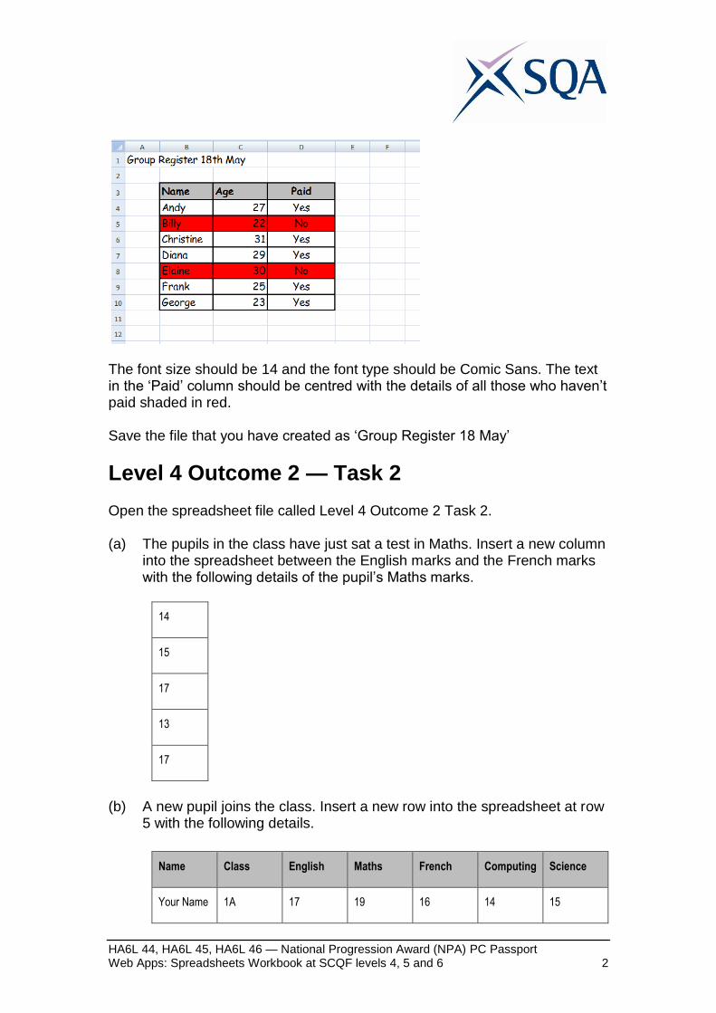
Open the spreadsheet file called Level 4 Outcome 2 Task 2. (a) The pupils in the class have just sat a test in Maths. Insert a new column
into the spreadsheet between the English marks and the French marks with the following details of the pupil’s Maths marks.
14
15
17
13
17
(b) A new pupil joins the class. Insert a new row into the spreadsheet at row
5 with the following details.
Name Class English Maths French Computing Science
Your Name 1A 17 19 16 14 15
HA6L 44, HA6L 45, HA6L 46 — National Progression Award (NPA) PC Passport Web Apps: Spreadsheets Workbook at SCQF levels 4, 5 and 6 3
(c) Using a function, calculate each pupil’s average mark across all the tests
that they have sat.
(d) Format this average mark rounded to a whole number (0 decimal places) and display this in green text.
(e) Each test is out of 20 marks. Using the pupil’s average mark, calculate their percentage score and display this in blue text.
(f) Print two copies of your spreadsheet:
(i) Showing the formulas used and the gridlines, using landscape orientation.
(ii) Showing the values stored and the column headings, using portrait orientation.
(g) Save a copy of this spreadsheet.
Level 4 Outcome 2 — Task 3
Open the spreadsheet file called Level 4 Outcome 2 Task 3. Using the data provided, create a bar chart to display the name of each dog and the number of walks that each dog needs.
Level 4 Outcome 3 — Task 1
Choose one of the spreadsheets that you have worked on in either Outcome 1 or Outcome 2. (a) Upload this spreadsheet to a cloud service, eg Google Drive, OneDrive
or DropBox.
(b) Share this spreadsheet with a colleague, this could be a fellow learner or your teacher/assessor and could be by e-mailing a link or through the use of social media.
(c) Act in a legal and ethical manner at all times.
Level 4 Outcome 3 — Task 2
Open the spreadsheet file called Level 4 Outcome 3 Task 2 and upload it to a cloud service. Add a comment to this file giving your answer to the question that it contains. Share this file with others in your class/group and ask them to comment with their views. Using your own answer and the input from others, enter your final answer in the space provided within the spreadsheet. Share your final answer with your teacher/assessor.
HA6L 44, HA6L 45, HA6L 46 — National Progression Award (NPA) PC Passport Web Apps: Spreadsheets Workbook at SCQF levels 4, 5 and 6 4
Level 5 Outcome 1 — Task 1
Open the spreadsheet file called Level 5 Outcome 1 Task 1. Using the key provided, change the colour of the cells to create a picture.
Level 5 Outcome 1 — Task 2
Open the spreadsheet file called Level 5 Outcome 1 Task 2. Find and fix the four errors in the spreadsheet. Add your name to the footer and print a copy of the corrected spreadsheet showing the formulas used.
Level 5 Outcome 1 — Task 3
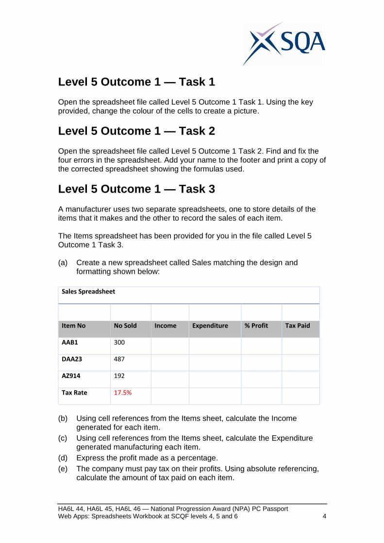
A manufacturer uses two separate spreadsheets, one to store details of the items that it makes and the other to record the sales of each item. The Items spreadsheet has been provided for you in the file called Level 5 Outcome 1 Task 3. (a) Create a new spreadsheet called Sales matching the design and
formatting shown below:
Sales Spreadsheet
Item No No Sold Income Expenditure % Profit Tax Paid
AAB1 300
DAA23 487
AZ914 192
Tax Rate 17.5%
(b) Using cell references from the Items sheet, calculate the Income
generated for each item.
(c) Using cell references from the Items sheet, calculate the Expenditure generated manufacturing each item.
(d) Express the profit made as a percentage.
(e) The company must pay tax on their profits. Using absolute referencing, calculate the amount of tax paid on each item.
HA6L 44, HA6L 45, HA6L 46 — National Progression Award (NPA) PC Passport Web Apps: Spreadsheets Workbook at SCQF levels 4, 5 and 6 5
(f) Calculate and display the following values:
(i) Total Pre-Tax Profit shaded in blue.
(ii) Total Tax Paid shaded in red.
(iii) Total Profit After Tax shaded in green.
(g) Ensure that all percentage and financial values are formatted correctly.
Level 5 Outcome 2 — Task 1
During the January sales a shop reduces all of its prices by 15%. Use a combination of absolute and relative referencing to enter formulas into the highlighted cells and complete the spreadsheet. (a) Open the spreadsheet file called Level 5 Outcome 2 Task 1.
(b) Format all the appropriate cells as currency.
(c) Calculate the amount of money saved on each item when the 15% discount is applied in the column ‘Discount Amount’
(d) Calculate the new price of each item in the column ‘New Price’
(e) Calculate the total amount of money saved if a customer was to buy all the items listed.
(f) Calculate the total bill for a customer buying all of the items listed.
Add your name to the header and print two copies of the completed spreadsheet, one displaying the values and the other displaying the formulas used.
HA6L 44, HA6L 45, HA6L 46 — National Progression Award (NPA) PC Passport Web Apps: Spreadsheets Workbook at SCQF levels 4, 5 and 6 6
Level 5 Outcome 2 — Task 2
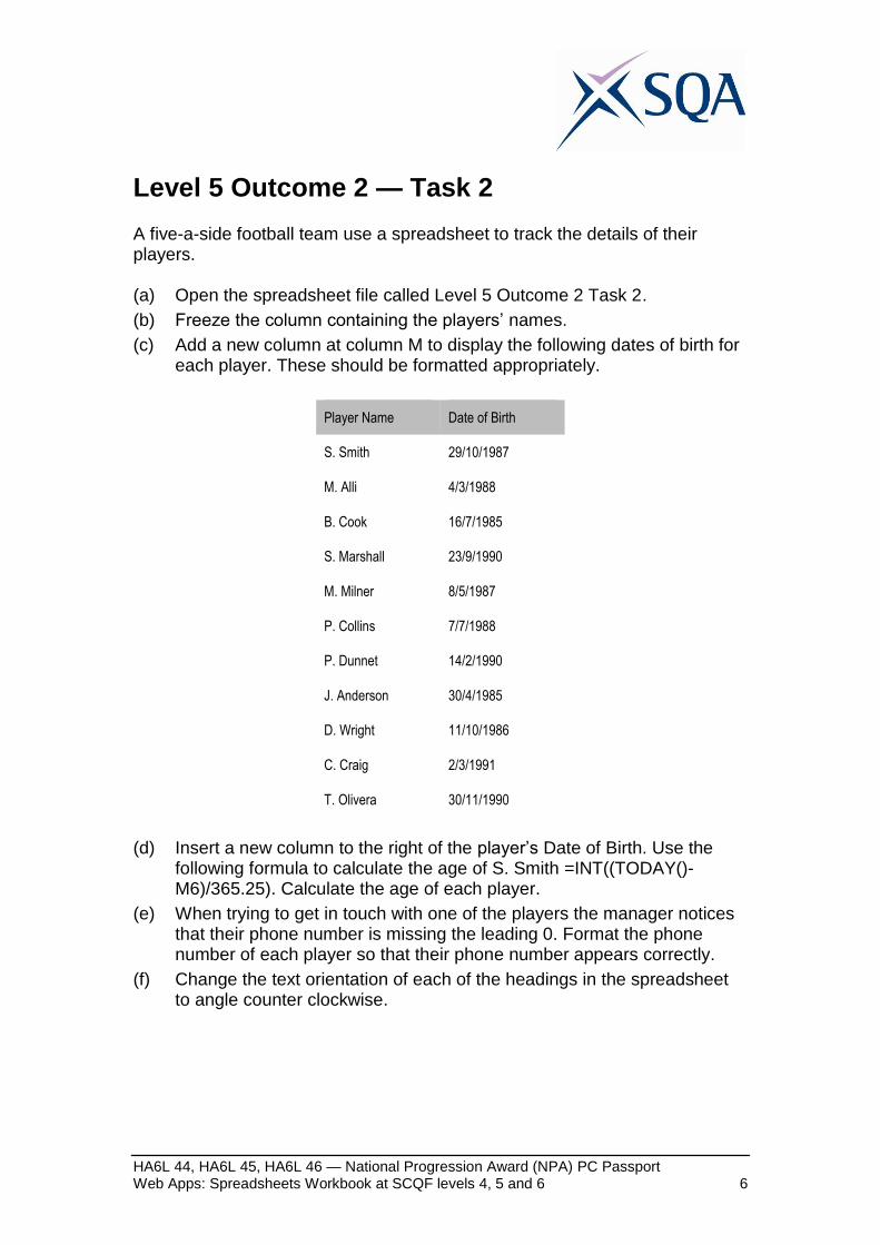
A five-a-side football team use a spreadsheet to track the details of their players. (a) Open the spreadsheet file called Level 5 Outcome 2 Task 2.
(b) Freeze the column containing the players’ names.
(c) Add a new column at column M to display the following dates of birth for each player. These should be formatted appropriately.
Player Name Date of Birth
S. Smith 29/10/1987
M. Alli 4/3/1988
B. Cook 16/7/1985
S. Marshall 23/9/1990
M. Milner 8/5/1987
P. Collins 7/7/1988
P. Dunnet 14/2/1990
J. Anderson 30/4/1985
D. Wright 11/10/1986
C. Craig 2/3/1991
T. Olivera 30/11/1990
(d) Insert a new column to the right of the player’s Date of Birth. Use the
following formula to calculate the age of S. Smith =INT((TODAY()-M6)/365.25). Calculate the age of each player.
(e) When trying to get in touch with one of the players the manager notices that their phone number is missing the leading 0. Format the phone number of each player so that their phone number appears correctly.
(f) Change the text orientation of each of the headings in the spreadsheet to angle counter clockwise.
HA6L 44, HA6L 45, HA6L 46 — National Progression Award (NPA) PC Passport Web Apps: Spreadsheets Workbook at SCQF levels 4, 5 and 6 7
(g) Change the formatting of the team’s name using the following
characteristics:
Font: Impact
Size: 28
Text Colour: red
Merge any cells required
(h) Apply a filter to each of the column headings. Use this filter to display only the players who are available for selection, hiding any players who are injured or suspended.
(i) Sort the data to display the players in ascending order of Squad Number.
(j) Calculate the team’s average overall rating correct to two decimal places.
HA6L 44, HA6L 45, HA6L 46 — National Progression Award (NPA) PC Passport Web Apps: Spreadsheets Workbook at SCQF levels 4, 5 and 6 8
Level 5 Outcome 2 — Task 3
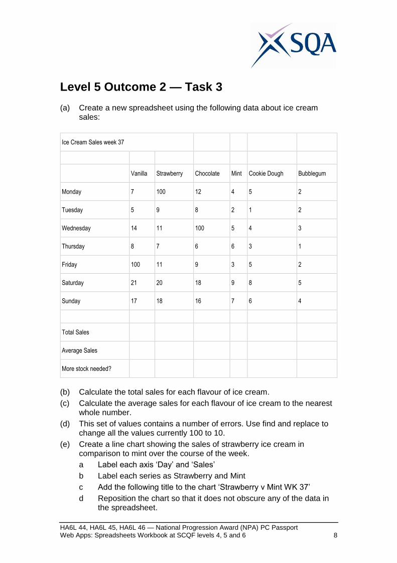
(a) Create a new spreadsheet using the following data about ice cream sales:
Ice Cream Sales week 37
Vanilla Strawberry Chocolate Mint Cookie Dough Bubblegum
Monday 7 100 12 4 5 2
Tuesday 5 9 8 2 1 2
Wednesday 14 11 100 5 4 3
Thursday 8 7 6 6 3 1
Friday 100 11 9 3 5 2
Saturday 21 20 18 9 8 5
Sunday 17 18 16 7 6 4
Total Sales
Average Sales
More stock needed?
(b) Calculate the total sales for each flavour of ice cream.
(c) Calculate the average sales for each flavour of ice cream to the nearest whole number.
(d) This set of values contains a number of errors. Use find and replace to change all the values currently 100 to 10.
(e) Create a line chart showing the sales of strawberry ice cream in comparison to mint over the course of the week.
a Label each axis ‘Day’ and ‘Sales’
b Label each series as Strawberry and Mint
c Add the following title to the chart ‘Strawberry v Mint WK 37’
d Reposition the chart so that it does not obscure any of the data in the spreadsheet.
HA6L 44, HA6L 45, HA6L 46 — National Progression Award (NPA) PC Passport Web Apps: Spreadsheets Workbook at SCQF levels 4, 5 and 6 9
e Change the colour of the strawberry line to red and the mint line to green.
(f) Popular flavours sell out quickly and the managers want to make sure that they always have each flavour of ice cream in stock. If a flavour has an average sale of more than 10 then more stock should be ordered. Use a conditional formula to display if more of each flavour is needed.
(g) Use cell protection to protect the entire sheet from any accidental edits.
(h) Add your name to the footer of the spreadsheet and print a copy so that the spreadsheet values and chart fit on a single sheet of paper.
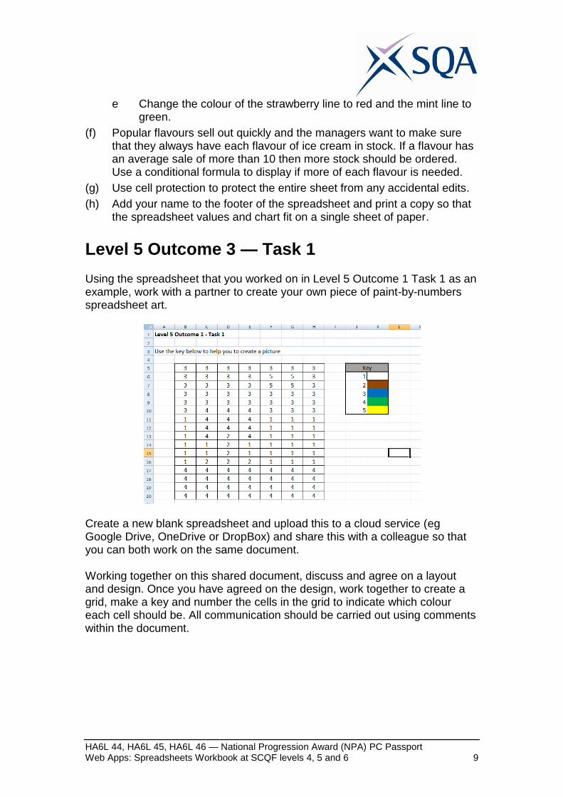
Level 5 Outcome 3 — Task 1
Using the spreadsheet that you worked on in Level 5 Outcome 1 Task 1 as an example, work with a partner to create your own piece of paint-by-numbers spreadsheet art.
Create a new blank spreadsheet and upload this to a cloud service (eg Google Drive, OneDrive or DropBox) and share this with a colleague so that you can both work on the same document. Working together on this shared document, discuss and agree on a layout and design. Once you have agreed on the design, work together to create a grid, make a key and number the cells in the grid to indicate which colour each cell should be. All communication should be carried out using comments within the document.
HA6L 44, HA6L 45, HA6L 46 — National Progression Award (NPA) PC Passport Web Apps: Spreadsheets Workbook at SCQF levels 4, 5 and 6 10
Share your completed number grid with another pair in your class/group and allow them to colour in the cells, following your key, to reveal the picture. When completing this task, make sure to work collaboratively and act legally and ethically.
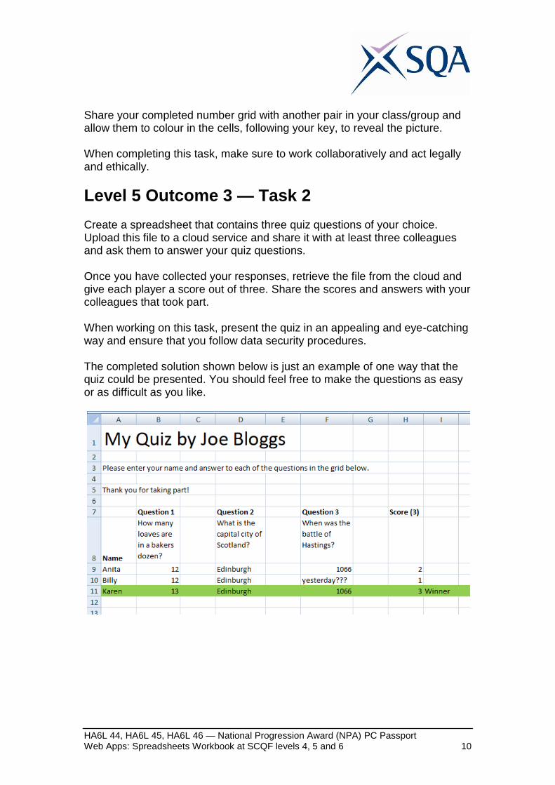
Level 5 Outcome 3 — Task 2
Create a spreadsheet that contains three quiz questions of your choice. Upload this file to a cloud service and share it with at least three colleagues and ask them to answer your quiz questions. Once you have collected your responses, retrieve the file from the cloud and give each player a score out of three. Share the scores and answers with your colleagues that took part. When working on this task, present the quiz in an appealing and eye-catching way and ensure that you follow data security procedures. The completed solution shown below is just an example of one way that the quiz could be presented. You should feel free to make the questions as easy or as difficult as you like.
HA6L 44, HA6L 45, HA6L 46 — National Progression Award (NPA) PC Passport Web Apps: Spreadsheets Workbook at SCQF levels 4, 5 and 6 11
Level 6 Outcome 1 — Task 1
A teacher uses a spreadsheet to track the progress of pupils in their class. A pupil’s progress is recoded three times per year; in September, December and February. A pupil’s progress can be rated as either: some progress, good progress or very good progress. (a) Create a spreadsheet to store the names of 10 pupils and track them
across the three tracking periods.
(b) Add data validation so that pupil’s progress can only be rated as some, good or very good. An appropriate error message should be displayed if the teacher tries to enter any invalid input.
(c) Use conditional formatting to colour code a pupil’s progress — very good in gold, good in silver and some in bronze.
(d) Gather evidence to show that you have tested that your spreadsheet functions correctly.
Level 6 Outcome 1 — Task 2
(a) Create a spreadsheet using the following data:
Manufacturer Model MegaPixels Zoom Price
Sony SON176 14 3x 99.99
Nikon NIK873 13 6x 109.99
Vivitar VIV909 14 4x 89.99
Canon CAN853 12 2x 85.50
Nikon NIK543 12 3x 84.99
Canon CAN187 10 4x 110.99
(b) Format the Price column as currency.
(c) Create a macro which changes the background colour and text colour of the data.
(d) Create a second macro to return the background colour to white and the text colour to black.
HA6L 44, HA6L 45, HA6L 46 — National Progression Award (NPA) PC Passport Web Apps: Spreadsheets Workbook at SCQF levels 4, 5 and 6 12
(e) Add a text box to the spreadsheet telling the user how to apply the
macros that you have created.
(f) Add an appropriate image to the spreadsheet. Resize and reposition the image if necessary.
Level 6 Outcome 2 — Task 1
A teacher records pupil’s feedback about how much they enjoyed a unit of programming using an online survey. This data is saved in a CSV file. (a) Open a blank spreadsheet and import the data from the file ‘L6 O2 Task
1.csv’
(b) Adjust the width of each column so that all the data is visible.
(c) Use search and replace to remove all of the date stamps contained in column A and column B.
(d) Insert a new column between column B and column C and calculate the time take to complete each questionnaire. Format this in seconds.
(e) Calculate the average time taken to complete the questionnaire. Format this is minutes and seconds.
(f) Count the number of pupils who found the test too hard.
(g) Pupils were asked to rate the unit between 1 (very bad) and 5 (very good). Pupils who enjoyed the unit are those who rated it as either 4 or 5. Count the number of pupils who enjoyed the class.
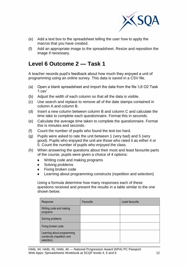
(h) When answering the questions about their most and least favourite parts of the course, pupils were given a choice of 4 options:
Writing code and making programs
Solving problems
Fixing broken code
Learning about programming constructs (repetition and selection)
Using a formula determine how many responses each of these questions received and present the results in a table similar to the one shown below.
Response Favourite Least favourite
Writing code and making programs
Solving problems
Fixing broken code
Learning about programming constructs (repetition and selection)
HA6L 44, HA6L 45, HA6L 46 — National Progression Award (NPA) PC Passport Web Apps: Spreadsheets Workbook at SCQF levels 4, 5 and 6 13
(i) Present this information in an appropriately labelled chart, comparing the
favourite and least favourite parts of the unit.
Level 6 Outcome 2 — Task 2
In hillwalking, a Munro is classified as any mountain over 3000 ft. A spreadsheet is used by a hillwalker to record the Munros that they have climbed.
Part 1
(a) Open the spreadsheet file called Level 6 Outcome 2 Task 2.
(b) Format the data in the spreadsheet as a table, choosing an appropriate banding and using the titles provided.
(c) Add a new column to your table to allow the hillwalker to add the date that they completed each Munro. Format this column as date.
(d) Add a new column to your table and use a formula to rank each Munro from highest (1) to lowest.
(e) Sort the Munros in order of their ranking from highest to lowest. Those with the same height should be sorted in ascending order of name.
(f) Use conditional formatting to highlight all the cells which are missing an OS Map number and Prefix.
Part 2
Outside your table, display the answers to the following questions using formulae:
The name and height of the 100th highest Munro
The name and height of the 200th highest Munro
Create a range of cells called ‘Top10’ covering the height of the 10 highest Munros in Scotland. Using this range, calculate and display the total height of these 10 Munros
HA6L 44, HA6L 45, HA6L 46 — National Progression Award (NPA) PC Passport Web Apps: Spreadsheets Workbook at SCQF levels 4, 5 and 6 14
Part 3
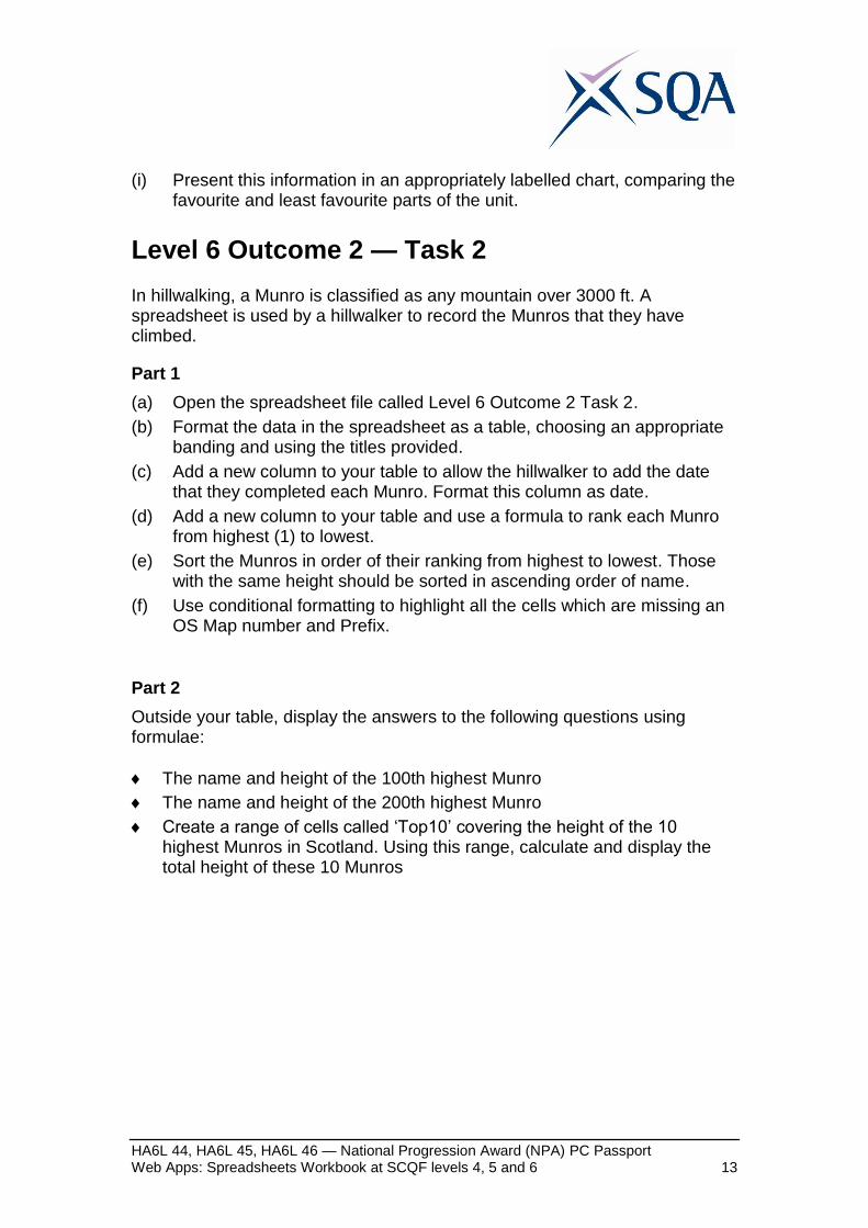
The Cuillin Ridge on the Isle of Skye (OS Map 32) consists of the following 11 Munros:
Sgurr Alasdair Sgurr nan Gillea Am Basteir
Sgurr Dearg - In Bruach na Frithe Sgurr nan Eag
Sgurr a'Ghreadai Sgurr Mhic Choin Sgurr a'Mhadaidh
Sgurr na Banachd Sgurr Dubh Mor
(a) Create a new table displaying the name and height in meters and gridref
of these Munros.
(b) Sort the table by their Gridref in ascending order.
(c) Create a line chart showing the ascent and descent of this ridge.
(d) Add appropriate titles to the chart. Re-position the chart on the sheet if required to ensure than no data values are hidden.
Part 4
The hillwalker has completed the following Munros on the following dates:
Ben Hope 27th April 2018
Ben Vane 1st Feb 2018
Driesh 19th March 2018
Ben Lomond 10th November 2017
Stob Ban 11th April 2017
Ben Lui 26th May 2017
(a) Update the data in your table.
(b) Use a formula to track the number of Munros the hillwalker has completed.
(c) Use a formula to track the number of Munros the hillwalker has still to complete.
(d) Sort the spreadsheet to show only the Munros the hillwalker has climbed, sorted in ascending order of height.
HA6L 44, HA6L 45, HA6L 46 — National Progression Award (NPA) PC Passport Web Apps: Spreadsheets Workbook at SCQF levels 4, 5 and 6 15
Level 6 Outcome 2 — Task 3
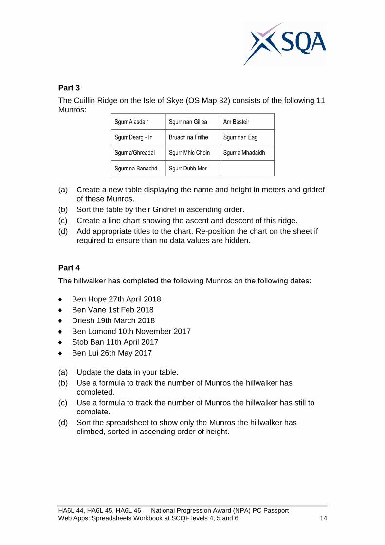
A spreadsheet is to be used to generate a user’s password based on their favourite word. (a) Create a spreadsheet using the following design:
Password Generator
Please enter your favourite word (must be
8 or more characters in length)
Start/end spaces
removed
Number of Characters
Random number
First three letters
capitalised
Final three letters in
lower case
Letter at position of
random number
Final Password
(b) Add validation to the cell where the user enters their favourite word. The
word must contain eight or more letters.
(c) Remove any spaces from the start or end of the word. Use this ‘clean’ version of the word for all subsequent tasks.
(d) Use a formula to calculate the number of letters in the word.
(e) Generate a random number between 1 and the number of letters in the word.
(f) Extract the first three letters from the start of the phrase and capitalise these letters.
HA6L 44, HA6L 45, HA6L 46 — National Progression Award (NPA) PC Passport Web Apps: Spreadsheets Workbook at SCQF levels 4, 5 and 6 16
(g) Extract the final three letters from the phrase and make sure that all three are lower case.
(h) Extract a letter from the position of the randomly generated number.
(i) Concatenate the following pieces of information, in the order below, to create the final password:
Last three letters
Number of characters in the word
Letter at the position of the random number
1st three letters (j) Lock the sheet so that the user is only able to enter their favourite word.
(k) Generate evidence showing that you have tested your password generator with at least three different words.
Level 6 Outcome 3 — Task 1
Work with a colleague to create an online coin toss game. Your game must include the following features: (a) Five rounds.
(b) A random number used to generate the result of each round, either heads or tails.
(c) A display of the result of each coin toss, either heads or tails.
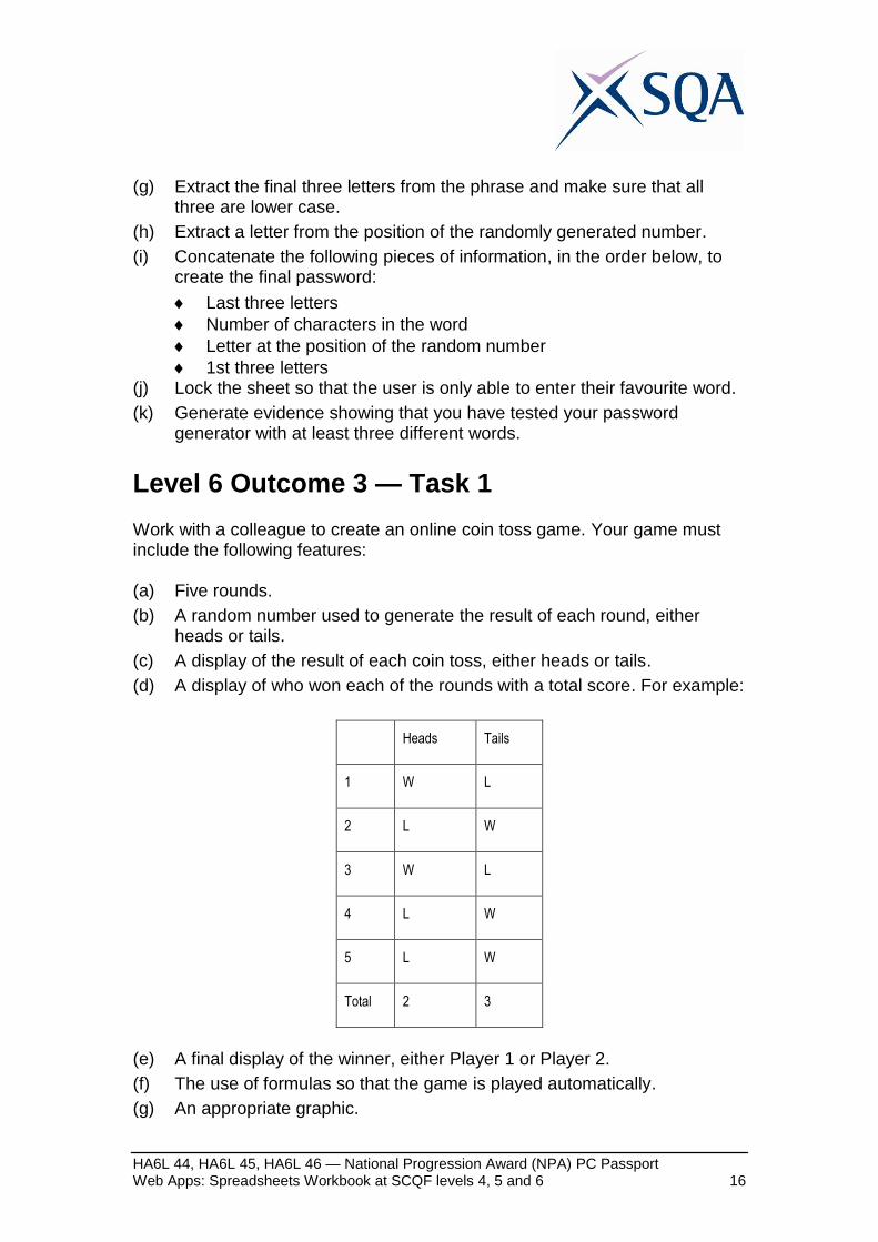
(d) A display of who won each of the rounds with a total score. For example:
Heads Tails
1 W L
2 L W
3 W L
4 L W
5 L W
Total 2 3
(e) A final display of the winner, either Player 1 or Player 2.
(f) The use of formulas so that the game is played automatically.
(g) An appropriate graphic.
HA6L 44, HA6L 45, HA6L 46 — National Progression Award (NPA) PC Passport Web Apps: Spreadsheets Workbook at SCQF levels 4, 5 and 6 17
(h) At least one additional feature agreed upon by the creators. A list of possible additional features is listed below:
Extend the game from 5 rounds to 10 rounds
Allow the user to enter their name and display the player name rather than Player 1 or Player 2
A bonus round worth double points
Each round being worth a different number of points, eg round 1 = 1 point, round 2 = 2 points, etc.
Any other additional feature of a similar level of difficulty The focus of this task is collaboration. It is important that decisions are discussed and agreed by both of the developers. All communication should take place through online comments/messages within the cloud service. All users must conduct themselves in a legal and ethical manner.
Level 6 Outcome 3 — Task 2
Part 1
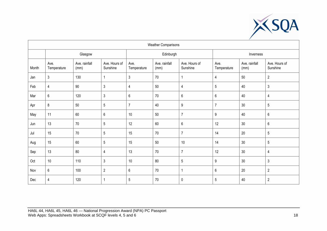
(a) Create a spreadsheet using the following data:
HA6L 44, HA6L 45, HA6L 46 — National Progression Award (NPA) PC Passport Web Apps: Spreadsheets Workbook at SCQF levels 4, 5 and 6 18
Weather Comparisons
Glasgow Edinburgh Inverness
Month Ave. Temperature
Ave. rainfall (mm)
Ave. Hours of Sunshine
Ave. Temperature
Ave. rainfall (mm)
Ave. Hours of Sunshine
Ave. Temperature
Ave. rainfall (mm)
Ave. Hours of Sunshine
Jan 3 130 1 3 70 1 4 50 2
Feb 4 90 3 4 50 4 5 40 3
Mar 6 120 3 6 70 6 6 40 4
Apr 8 50 5 7 40 9 7 30 5
May 11 60 6 10 50 7 9 40 6
Jun 13 70 5 12 60 6 12 30 6
Jul 15 70 5 15 70 7 14 20 5
Aug 15 60 5 15 50 10 14 30 5
Sep 13 80 4 13 70 7 12 30 4
Oct 10 110 3 10 80 5 9 30 3
Nov 6 100 2 6 70 1 6 20 2
Dec 4 120 1 5 70 0 5 40 2
HA6L 44, HA6L 45, HA6L 46 — Web Apps: Spreadsheets Workbook for National Progression Award in PC Passport at SCQF levels 4, 5 and 6 19
(b) Using formulas, carry out the following calculations:
(i) The average temperature for each city over the 12 months, rounded to one decimal place.
(ii) The total of the average rainfall for each city.
(iii) The value of the highest hours of sunshine for each city.
(c) Use a chart of your choice to represent any of the data in the spreadsheet in a graphical format.
(d) Save this version of your spreadsheet as ‘L6 Outcome 3 Task 2 Solution’
Part 2
(a) Make a copy of your worksheet and intentionally introduce three errors into the sheet. At least one error should be with a formula and at least one error should be in the chart.
These errors could include:
An error in a formula, eg incorrect cells/range, incorrect sign, incorrect function, etc.
An error in the chart, eg incorrect range, incorrect axis label(s), incorrect heading, etc.
(b) Save this version of your spreadsheet as ‘L6 Outcome 3 Task 2 with Errors’
Part 3
(a) Upload the version of the sheet that contains the errors (Part 2) to a cloud service and share it with a colleague and ask them to find and fix the errors.
(b) Provide feedback to your colleague about their progress as they complete the task, informing them of how they are progressing finding and fixing the errors. This may include providing your colleague with hints to help them identify the errors if they are stuck.
(c) Share the solution spreadsheet (Part 1) with your colleague to allow your colleague to check their answers against the solution.
(d) Adhere to data security requirements and procedures by acting legally and ethically.


![5 refreshed PC Passport [Read-Only] · PC Passport (Intermediate) unitsPC Passport (Intermediate) units IT Systems 5 F1FA 11 0.5 IT Software - Spreadsheets 5 F1FC 11 1 and Database](https://img.pdfslide.us/doc/110x75/5fd402c3a70543283605b610/5-refreshed-pc-passport-read-only-pc-passport-intermediate-unitspc-passport.jpg)