Embed Size (px)
Citation preview

Nozzle Study
Yan Zhan, Foluso Ladeinde
April , 2011
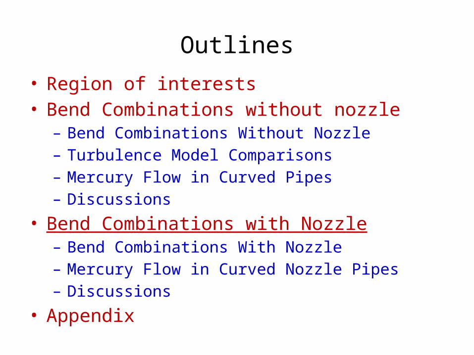
Outlines• Region of interests• Bend Combinations without nozzle– Bend Combinations Without Nozzle– Turbulence Model Comparisons– Mercury Flow in Curved Pipes – Discussions
• Bend Combinations with Nozzle– Bend Combinations With Nozzle– Mercury Flow in Curved Nozzle Pipes – Discussions
• Appendix
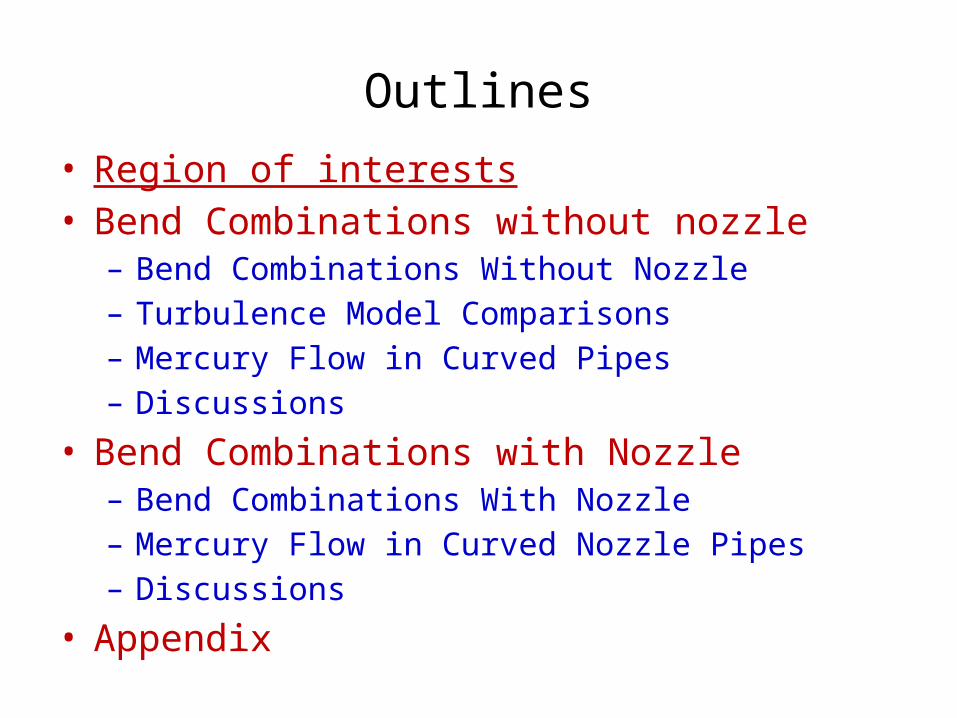
Region of interests
Hg delivery system at CERN
Simulation Regime
Interests: Influence of nozzle & nozzle upstream on the jet exit

Outlines• Region of interests• Bend Combinations without nozzle– Bend Combinations Without Nozzle– Turbulence Model Comparisons– Mercury Flow in Curved Pipes – Discussions
• Bend Combinations with Nozzle– Bend Combinations With Nozzle– Mercury Flow in Curved Nozzle Pipes – Discussions
• Appendix

Bend Combinations Without Nozzle (1)
Geometry of bends with varying anglesNondimensionalized by pipe diameter (p.d.);φ range: 0⁰, 30⁰, 60⁰, 90⁰.
Mesh at the cross-sectionnr × nθ =152×64 (the 1st grid center at y+≈1)
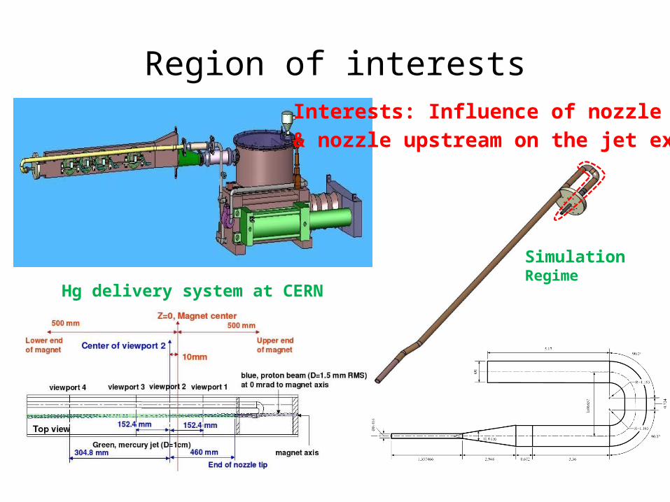
Geometries without nozzle: (a) 0⁰/0⁰ ; (b) 30⁰/30⁰; (c) 60⁰/60⁰; (d) 90⁰/90⁰ nx =40 +nφ+20+ nφ +100where nφ depends on the bend angle φ
Bend Combinations Without Nozzle (2)(a)
(b) (c)
(d)
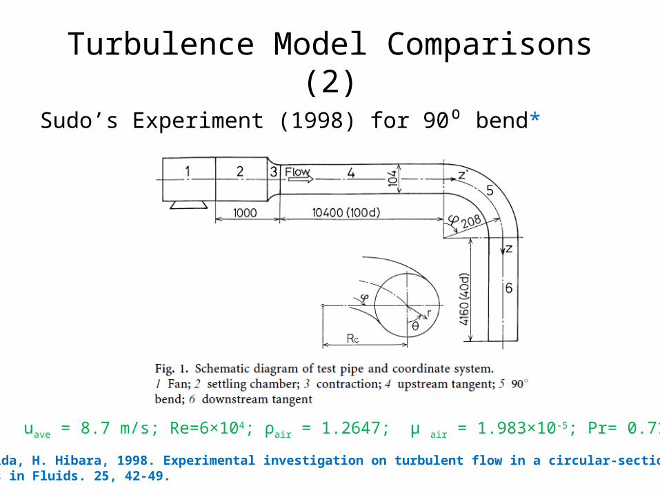
Turbulence Model Comparisons (2)
Sudo’s Experiment (1998) for 90⁰ bend*
•K. Sudo, M. Sumida, H. Hibara, 1998. Experimental investigation on turbulent flow in a circular-sectioned 90-degrees bend, Experiments in Fluids. 25, 42-49.
uave = 8.7 m/s; Re=6×10⁴; ρair = 1.2647; μ air = 1.983×10⁻⁵; Pr= 0.712
Inlet
Outlet
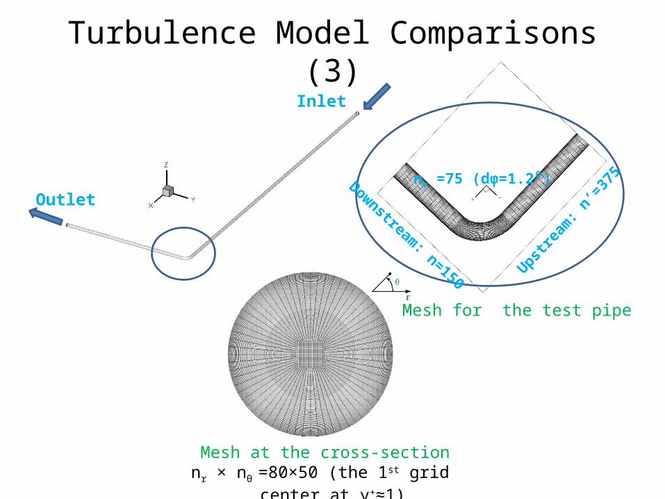
Turbulence Model Comparisons (3)
Mesh at the cross-sectionnr × nθ =80×50 (the 1st grid center at y+≈1)
Mesh for the test pipe
Upstream: n
’=375Downstream: n=150
nφ =75 (dφ=1.2⁰)
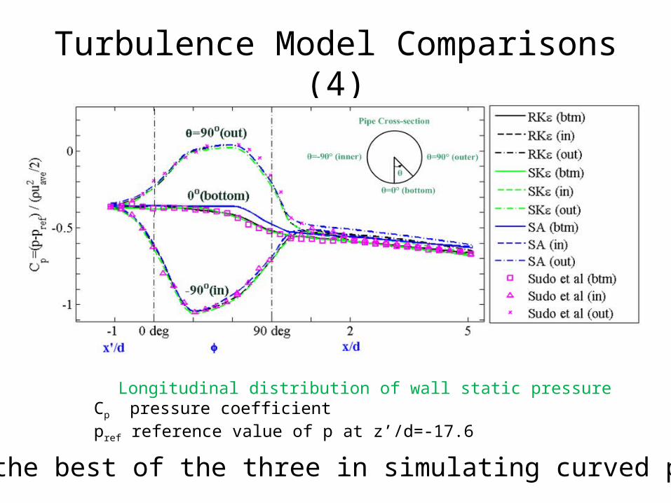
Turbulence Model Comparisons (4)
Longitudinal distribution of wall static pressureCp pressure coefficientpref reference value of p at z’/d=-17.6
RKε is the best of the three in simulating curved pipe flow
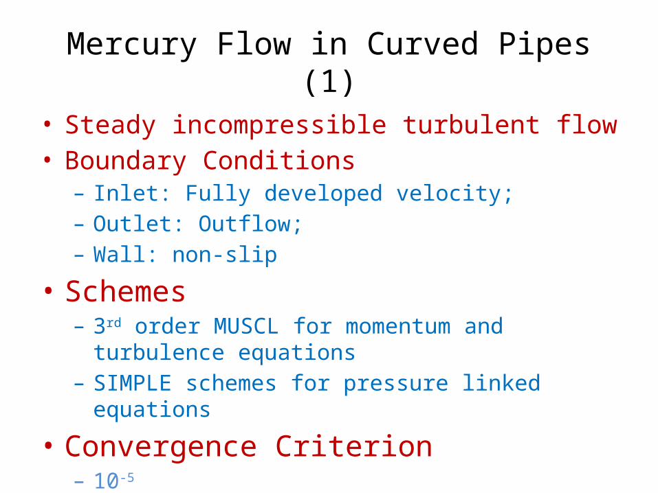
Mercury Flow in Curved Pipes (1)
• Steady incompressible turbulent flow• Boundary Conditions– Inlet: Fully developed velocity;– Outlet: Outflow;– Wall: non-slip
• Schemes– 3rd order MUSCL for momentum and turbulence equations– SIMPLE schemes for pressure linked equations
• Convergence Criterion– 10-5
Mercury Flow in Curved Pipes (2)
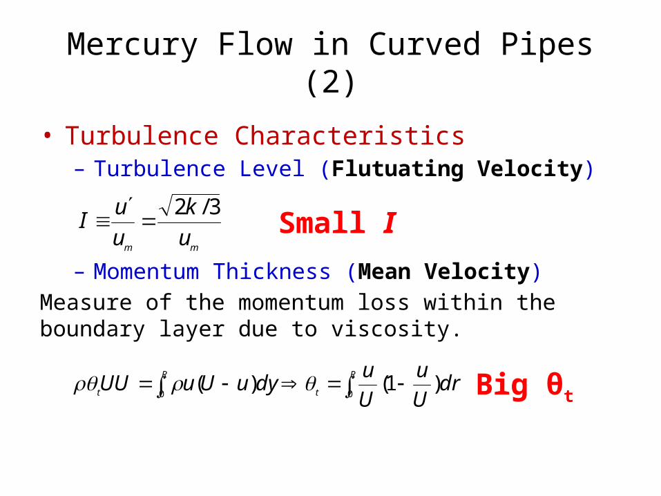
• Turbulence Characteristics– Turbulence Level (Flutuating Velocity)
– Momentum Thickness (Mean Velocity)Measure of the momentum loss within the boundary layer due to viscosity.
mmu
k
u
uI
3/2
R
t
R
tdr
U
u
U
udyuUuUU
00)1( )(
Small I
Big θt
Mercury Flow in Curved Pipes (3)
• Turbulence Level (1)
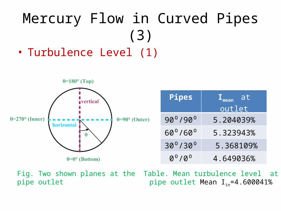
Fig. Two shown planes at the pipe outlet
Pipes Imean at outlet
90 /90⁰ ⁰ 5.204039%
60 /60⁰ ⁰ 5.323943%
30 /30⁰ ⁰ 5.368109%
0 /0⁰ ⁰ 4.649036%
Table. Mean turbulence level at pipe outlet Mean Iin=4.600041%
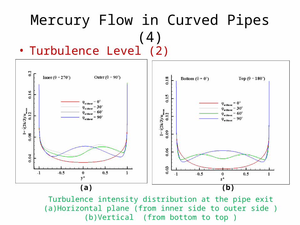
Mercury Flow in Curved Pipes (4)• Turbulence Level (2)
Turbulence intensity distribution at the pipe exit(a) Horizontal plane (from inner side to outer side )
(b) Vertical (from bottom to top )
(a) (b)
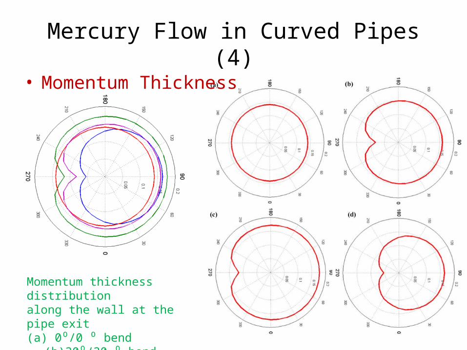
Mercury Flow in Curved Pipes (4)• Momentum Thickness
Momentum thickness distributionalong the wall at the pipe exit(a) 0⁰/0 ⁰ bend (b)30⁰/30 ⁰ bend (c) 60⁰/60 ⁰ bend (d) 90⁰/90 ⁰ bend
Discussions
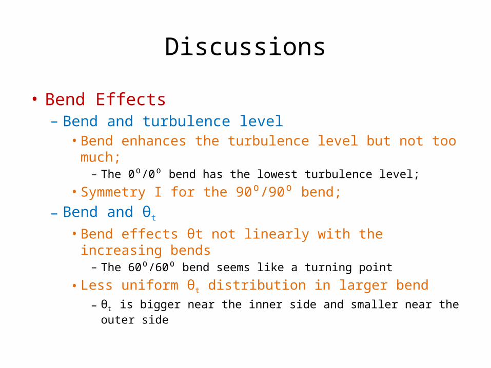
• Bend Effects– Bend and turbulence level• Bend enhances the turbulence level but not too much;
– The 0⁰/0⁰ bend has the lowest turbulence level;
• Symmetry I for the 90⁰/90⁰ bend;
– Bend and θt
• Bend effects θt not linearly with the increasing bends– The 60⁰/60⁰ bend seems like a turning point
• Less uniform θt distribution in larger bend– θt is bigger near the inner side and smaller near the outer side
Outlines• Region of interests• Bend Combinations without nozzle– Bend Combinations Without Nozzle– Turbulence Model Comparisons– Mercury Flow in Curved Pipes – Discussions
• Bend Combinations with Nozzle– Bend Combinations With Nozzle– Mercury Flow in Curved Nozzle Pipes – Discussions
• Appendix
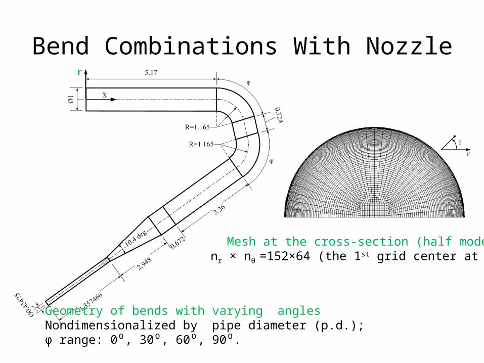
Bend Combinations With Nozzle
Geometry of bends with varying anglesNondimensionalized by pipe diameter (p.d.);φ range: 0⁰, 30⁰, 60⁰, 90⁰.
Mesh at the cross-section (half model)nr × nθ =152×64 (the 1st grid center at y+≈1)
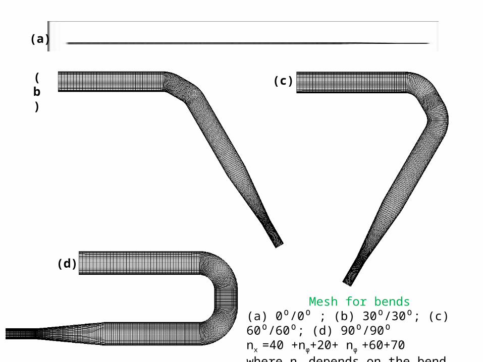
Mesh for bends(a) 0⁰/0⁰ ; (b) 30⁰/30⁰; (c) 60⁰/60⁰; (d) 90⁰/90⁰ nx =40 +nφ+20+ nφ +60+70where nφ depends on the bend angle φ
(a)
(b) (c)
(d)
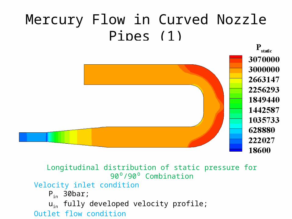
Mercury Flow in Curved Nozzle Pipes (1)
Longitudinal distribution of static pressure for 90⁰/90⁰ CombinationVelocity inlet condition
Pin 30bar;uin fully developed velocity profile;
Outlet flow condition
Mercury Flow in Curved Nozzle Pipes (2)
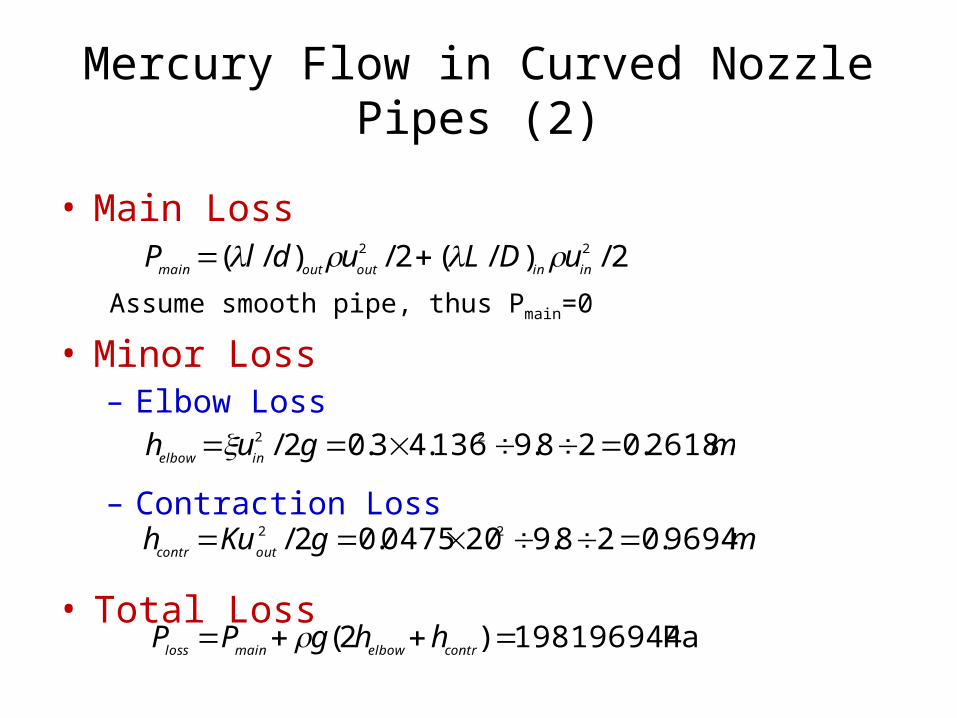
• Main Loss
Assume smooth pipe, thus Pmain=0
• Minor Loss– Elbow Loss
– Contraction Loss
• Total Loss
2/)/(2/)/( 22
ininoutoutmainuDLudlP
mguhinelbow
2618.028.9136.43.02/ 22
mgKuhoutcontr
9694.028.9200475.02/ 22
Pa 198196944 )2( contrelbowmainlosshhgPP
Mercury Flow in Curved Nozzle Pipes (3)
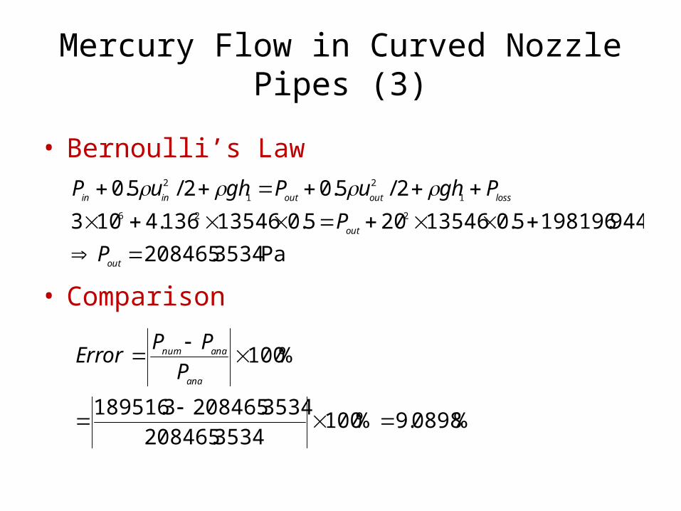
• Bernoulli’s Law
• Comparison
Pa 3534.208465
944.1981965.013546205.013546136.410 3
2/5.02/5.0226
1
2
1
2
out
out
lossoutoutinin
P
P
PghuPghuP
%0898.9%1003534.208465
3534.2084653.189516
%100
ana
ananum
P
PPError
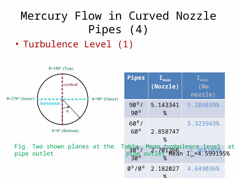
Mercury Flow in Curved Nozzle Pipes (4)
• Turbulence Level (1)
Pipes Imean
(Nozzle)Imean
(No nozzle)
90 /90⁰ ⁰ 5.143341% 5.204039%
60 /60⁰ ⁰ 2.858747% 5.323943%
30 /30⁰ ⁰ 2.701366% 5.368109%
0 /0⁰ ⁰ 2.182027% 4.649036%
Fig. Two shown planes at the pipe outlet Table. Mean turbulence level at pipe outlet Mean Iin=4.599195%
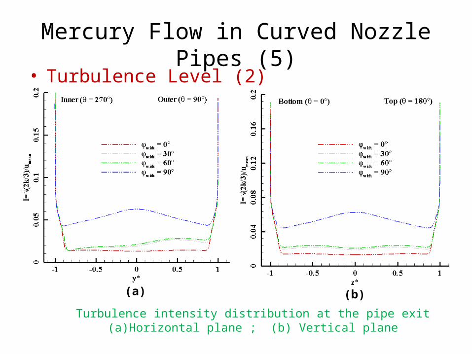
Mercury Flow in Curved Nozzle Pipes (5)• Turbulence Level (2)
Turbulence intensity distribution at the pipe exit(a) Horizontal plane ; (b) Vertical plane
(a) (b)
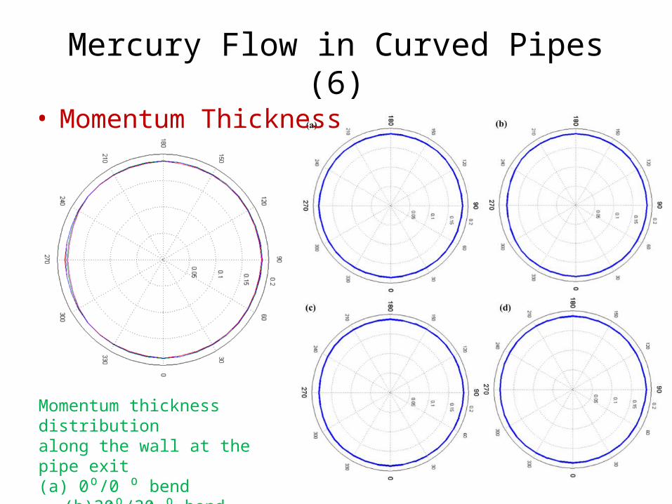
Mercury Flow in Curved Pipes (6)• Momentum Thickness
Momentum thickness distributionalong the wall at the pipe exit(a) 0⁰/0 ⁰ bend (b)30⁰/30 ⁰ bend (c) 60⁰/60 ⁰ bend (d) 90⁰/90 ⁰ bend
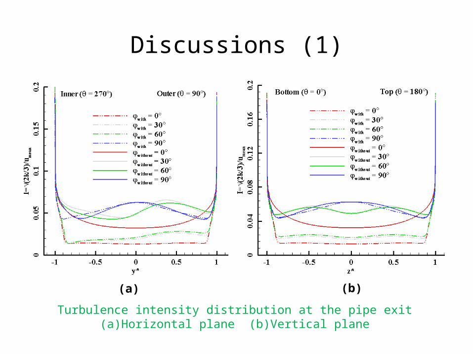
Discussions (1)
Turbulence intensity distribution at the pipe exit(a) Horizontal plane (b)Vertical plane
(a) (b)
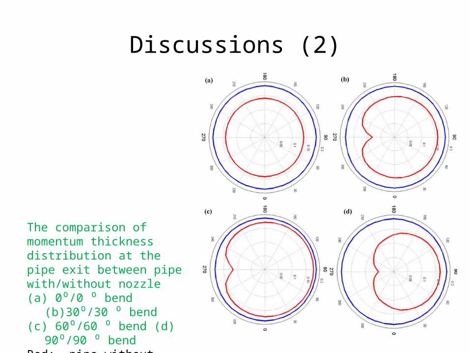
Discussions (2)
The comparison of momentum thickness distribution at the pipe exit between pipe with/without nozzle(a) 0⁰/0 ⁰ bend (b)30⁰/30 ⁰ bend (c) 60⁰/60 ⁰ bend (d) 90⁰/90 ⁰ bendRed: pipe without nozzle;Blue: pipe with nozzle.
Discussions (3)
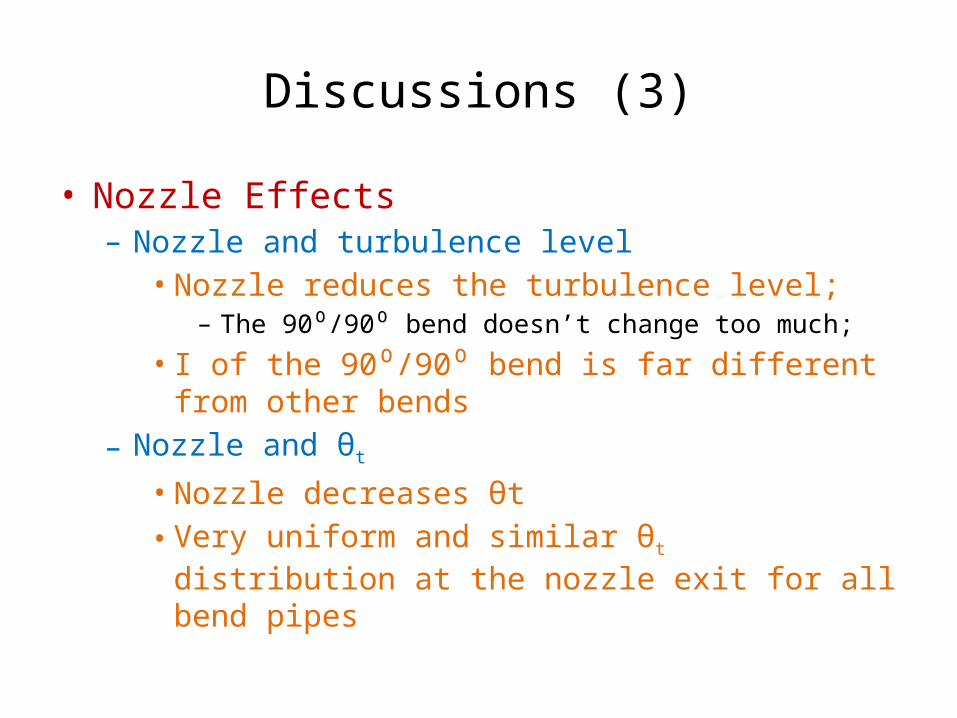
• Nozzle Effects– Nozzle and turbulence level• Nozzle reduces the turbulence level;
– The 90⁰/90⁰ bend doesn’t change too much;
• I of the 90⁰/90⁰ bend is far different from other bends– Nozzle and θt
• Nozzle decreases θt• Very uniform and similar θt distribution at the nozzle
exit for all bend pipes
Outlines• Region of interests• Bend Combinations without nozzle– Bend Combinations Without Nozzle– Turbulence Model Comparisons– Mercury Flow in Curved Pipes – Discussions
• Bend Combinations with Nozzle– Bend Combinations With Nozzle– Mercury Flow in Curved Nozzle Pipes – Discussions
• Appendix
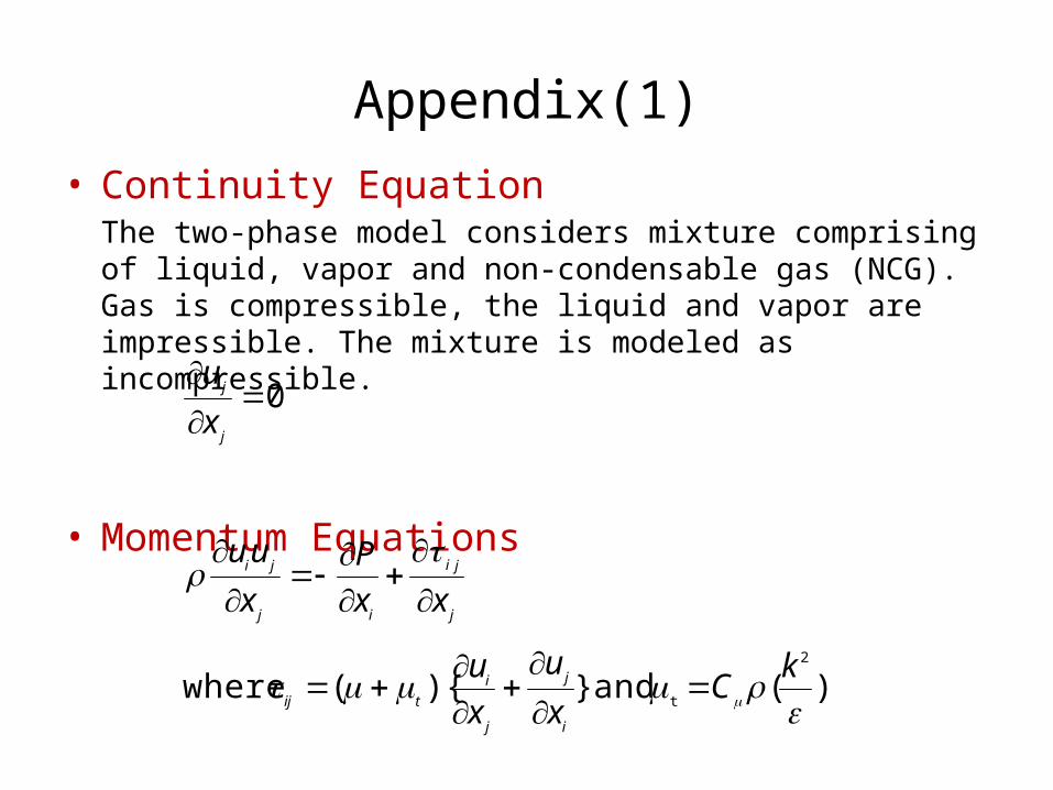
Appendix(1)• Continuity Equation
The two-phase model considers mixture comprising of liquid, vapor and non-condensable gas (NCG). Gas is compressible, the liquid and vapor are impressible. The mixture is modeled as incompressible.
• Momentum Equations
0
j
j
x
u
j
ji
ij
ji
xx
P
x
uu
)( and }){( where2
t
kC
x
u
x
u
i
j
j
i
tij
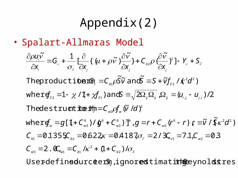
Appendix(2)
• Spalart-Allmaras Model
~
2
2
~
])~
(}~
)~{([1~
SYx
Cxx
Gx
u
j
b
jji
i
)/(~~ and ~~
termproduction The 22
2~1dfvSSvSCG
vb
2
1)/~( n termdestructio The dvfCY
ww
3.0,1.7 2/3, ,4187.0,622.0,1355.021~21
wvbbCCCC
2/)(,2 and )1/(1 where,,1~2~ ijjiijijijvv
uuSff
)~
/(~ ),( ,)]/()1[( where 226
2
6/16
3
66
3dSvrrrCrgCgCgf
wwww
vbbwwCCCC ~2
2
113/)1(/2.0,
stresses Reynolds theestimating ignored , termsource defined-UservS
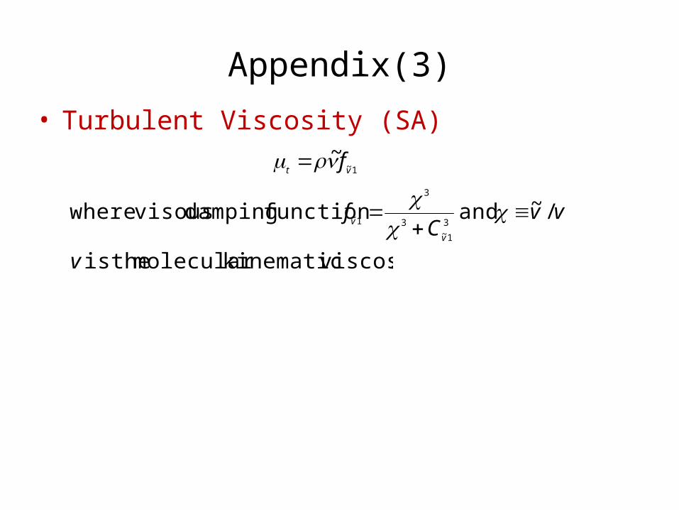
Appendix(3)• Turbulent Viscosity (SA)
vvC
fv
v/~ and function damping visouswhere
3
1~3
3
1~
1~
~vtf
. viscositykinematicmolecular theis v
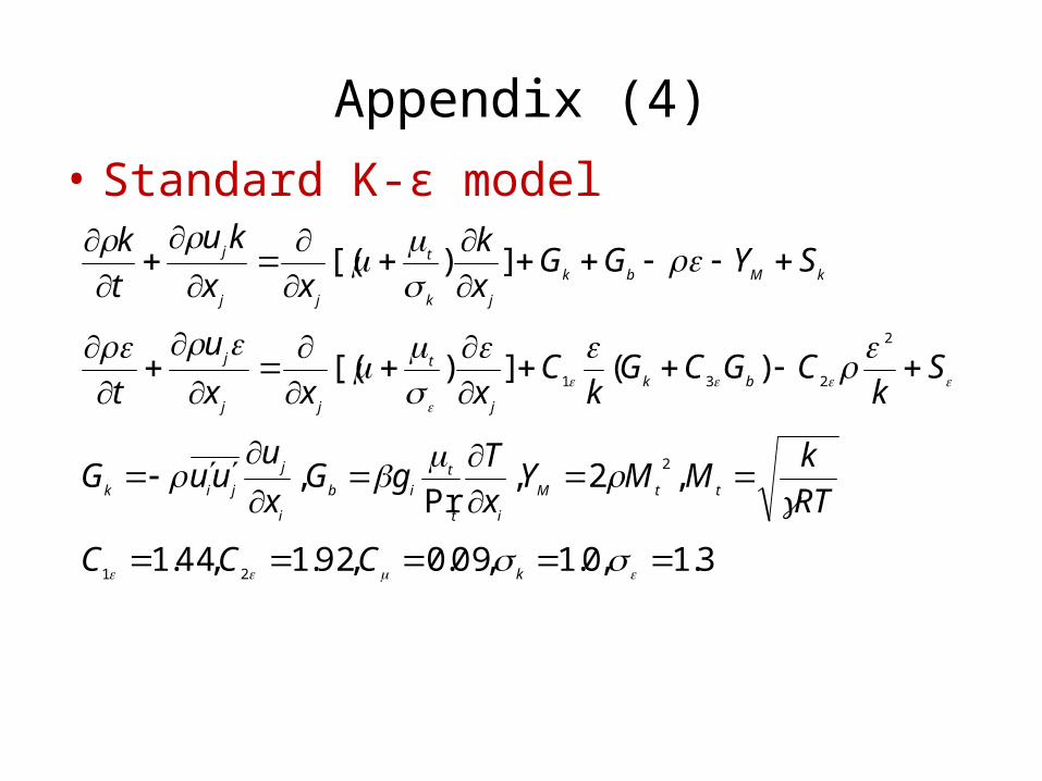
Appendix (4)• Standard K-ε model
S
kCGCG
kC
xxx
u
t bk
j
t
jj
j
2
231)(])[(
kMbk
jk
t
jj
j SYGGx
k
xx
ku
t
k
])[(
RT
kMMY
x
TgG
x
uuuG
ttM
it
t
ib
i
j
jik
,2,Pr
,2
3.1,0.1,09.0,92.1,44.121
k
CCC
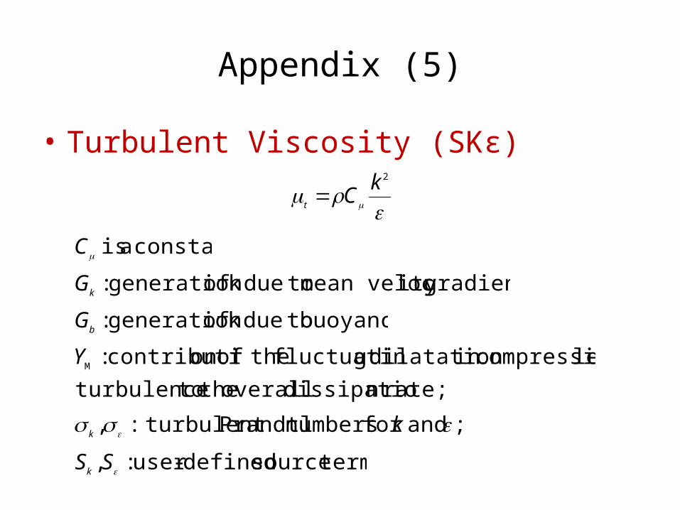
Appendix (5)
• Turbulent Viscosity (SKε)
2kC
t
constant. a is C
gradients;ity mean veloc toduek of generation :k
G
buoyance; toduek of generation :b
G
rate;n dissipatio overall the toturbulence
lecompressibin dilatation gfluctuatin theofon contributi :MY
; and for numbers Prandtl turbulent:, kk
terms;source defined-user :, SSk
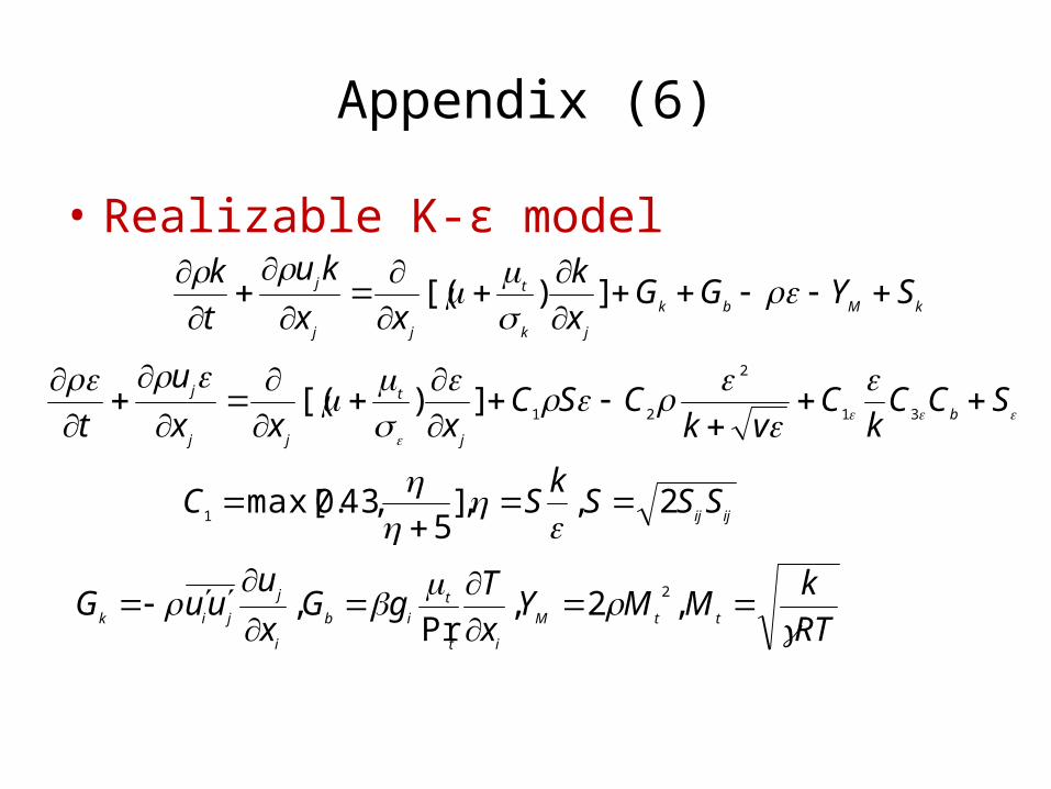
Appendix (6)
• Realizable K-ε model
kMbk
jk
t
jj
j SYGGx
k
xx
ku
t
k
])[(
SCC
kC
vkCSC
xxx
u
t b
j
t
jj
j
31
2
21])[(
ijijSSS
kSC 2,,]
5,43.0max[
1
RT
kMMY
x
TgG
x
uuuG
ttM
it
t
ib
i
j
jik
,2,Pr
,2
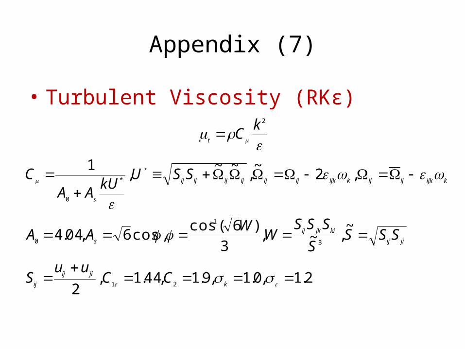
Appendix (7)
• Turbulent Viscosity (RKε)
2kC
t
kijkijijkijkijijijijijij
s
SSUkU
AAC
,2~
,~~
,1 *
*
0
jiij
kijkij
sSSS
S
SSSW
WAA
~,~,
3
)6(cos,cos6,04.4
3
1
0
2.1,0.1,9.1,44.1,2 21
k
jiij
ijCC
uuS
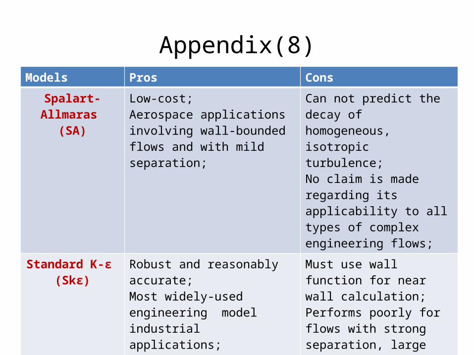
Appendix(8)Models Pros Cons
Spalart-Allmaras (SA)
Low-cost;Aerospace applications involving wall-bounded flows and with mild separation;
Can not predict the decay of homogeneous, isotropic turbulence; No claim is made regarding its applicability to all types of complex engineering flows;
Standard K-ε (Skε)
Robust and reasonably accurate;Most widely-used engineering model industrial applications;Contains submodels for buoyancy, compressibility, combustion, etc;
Must use wall function for near wall calculation;Performs poorly for flows with strong separation, large streamline curvature, and �large pressure gradient;
Realizable K-ε (Rkε)
superior performance for flows involving rotation, boundary �layers under strong adverse pressure gradients, separation, and recirculation
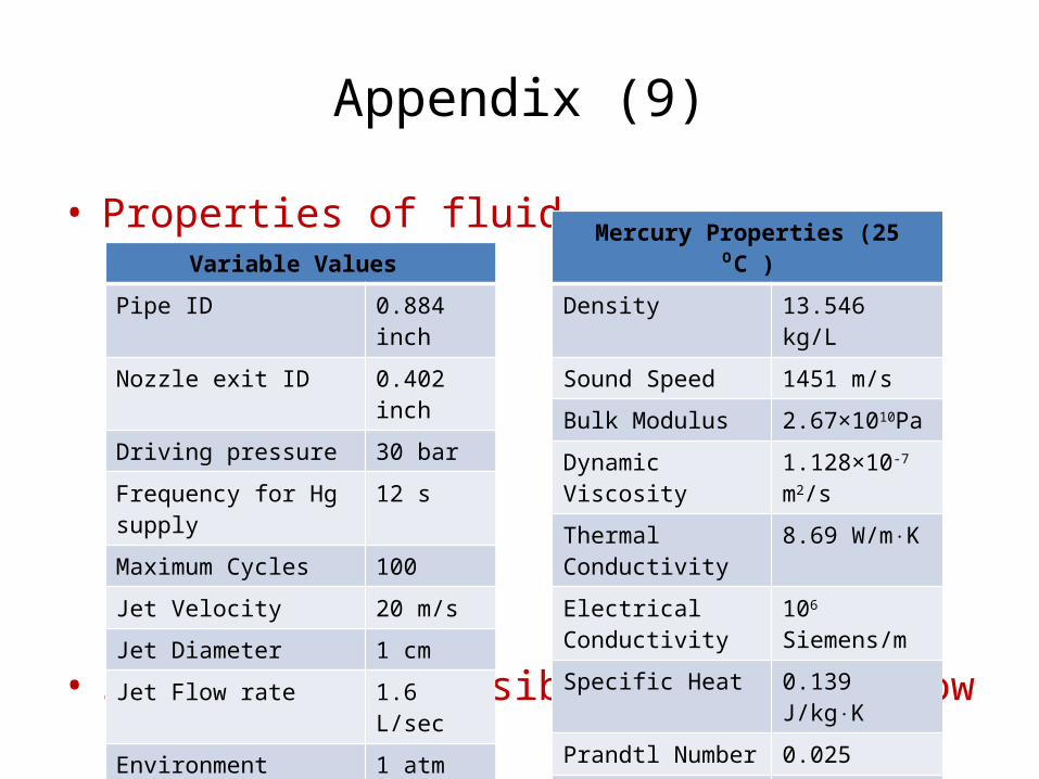
Appendix (9)
• Properties of fluid
• Steady incompressible turbulent flow
Variable Values
Pipe ID 0.884 inch
Nozzle exit ID 0.402 inch
Driving pressure 30 bar
Frequency for Hg supply 12 s
Maximum Cycles 100
Jet Velocity 20 m/s
Jet Diameter 1 cm
Jet Flow rate 1.6 L/sec
Environment 1 atm air/vacuum
Mercury Properties (25 C )⁰
Density 13.546 kg/L
Sound Speed 1451 m/s
Bulk Modulus 2.67×10¹⁰Pa
Dynamic Viscosity 1.128×10⁻⁷ m2/s
Thermal Conductivity
8.69 W/m K⋅
Electrical Conductivity
106 Siemens/m
Specific Heat 0.139 J/kg K⋅
Prandtl Number 0.025
Surface Tension 465 dyne/cm