Nowcasting GDP directional change with an … · Nowcasting GDP directional change with an application to French business survey data Matthieu Cornec and annFy Mikol INSEE Business

Nowcasting GDP directional change with an

application to French business survey data

Matthieu Cornec and Fanny Mikol

INSEE Business Surveys Unit

Directorate of economic studies and summaries

Timbre G120

15 Boulevard Gabriel Peri 92245 Malako� Cedex, France

June 06, 2011

Abstract

Despite a rich litterature on GDP growth level forecasting, few studies

have focused on forecasting GDP directional change. This is all the more

suprising that economic outlook analysis is mainly explained in terms of

acceleration or deceleration. We conduct a comparative study between

di�erent class of models ranging from econometrics to machine learning.

Empirical investigations on French economy suggest that classi�cation

models slightly outperform their level-based counterpart, with the respect

to the sign forecast exercise. We also provide analytical properties for

future model-based predictions. Eventually, we construct a directional

risk index which describes in probability terms the risk of an upcoming

deceleration. Applied to the balances of di�erent business surveys, it

appears as a useful tool for economic forecasters.

Keywords: Macroeconomic Forecasts, forecasts evaluation, directional forecast,classi�cation.

1

1 Introduction

In many �elds of studies, observations must be classi�ed into two di�erentsgroups. Here are some examples of classi�cation problems:

• predict if patient, hospitalized for a heart attack, will have a second heartattack. The classi�cation can be based on clinical measurements.

• predict if an internaut will buy a product on a website, knowing his income,his age,...

• guess the number of a handwritten code from a digitized image.

For their nowcasting exercise, economists have mainly focused on point forecast,rather than on directional change forecast (or sign forecast). For example, inthe Note de Conjoncture [6], the GDP growth forecast for the �ash estimateof Q1 2011 was 0.6%. An abundant litterature on level forecasts has �ourishedover the past decades (see [13, 19, 16] and references therein). For the Frencheconomy, we can quote [1, 7, 5].

Surprisingly, there are few studies examining the predictability of the sign ofGDP growth movement. Methodology for sign forecast evaluation was �rst in-troduced for market timing in [12, 9] and for macroeconomic forecasts in [18, 15].A nonparametric test of predictive performance can be found in [14]. For ex-ample, [16] use [14] test to investigate the ability of their level based modelsto predict GDP directional change from one quarter to another. This lack ofempirical studies is all the more surprising that, at the same time, economicforecasters describe their baselined scenario in terms of acceleration or decelera-tion: �production accelerates�, �activity slows down�, �business climate remainsstable�. This qualitative economic analysis is mainly supported by two reasons.First, this realistic view acknowledges that nobody can predict future evolutionof the economic outlook with absolute certainty (see for a detailed review ondensity forecast [19]). Secondly, while accuracy, as measured by quantitativeerrors, is important, it may be even more crucial to accurately forecast the signof change (see [17]). Will real GDP accelerate (or decelerate)? Economists thusunderline the main direction of the economy. In other words, their review refersimplictly to a sign forecast.

The purpose of this paper is threefold. First, to provide a sequential frameworkto analyse sign forecasts. Indeed, the forecasting exercise is made sequentiallyon the basis of real time data. Our framework di�ers from previous studies intwo main points: it is model free -to allow a large class of predictors- and nonasymptotic -since in practice, the number of GDP forecasts are rather limited-. The procedure to test whether forecasts are useful is based on a comparisonwith naive uninformed benchmarks. Second, we conduct an empirical compara-tive study between classi�cation models, including linear discriminant analysis,support vector machine, regression trees and level-based models including like

2

regression. Eventually, we construct a pro�le index which describes in proba-bility terms the risk of an upcoming deceleration.

This paper is organised as follows. Section 2 describes our data sets and de�nesthe problem set up. In section 3, we conduct a comparative empirical studyfor a wide range of methods from econometrics to machine learning theory.In Section 4, we derive analytical properties for future sign forecasts, namelyasymptotic and non asymptotic con�dence interval. Eventually, in section 5,we construct our directional risk index to describe in probability terms theuncertainty associated to our sign forecast.

2 Data description and problem set up

Flash estimate

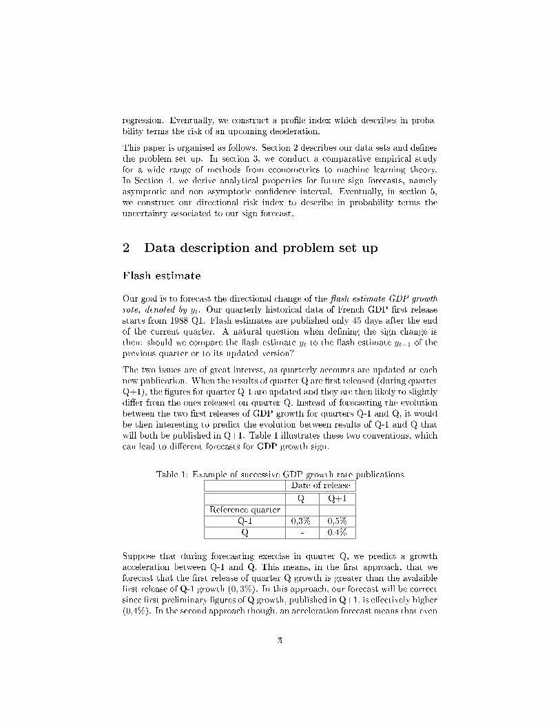
Our goal is to forecast the directional change of the �ash estimate GDP growthrate, denoted by yt. Our quarterly historical data of French GDP �rst releasestarts from 1988 Q1. Flash estimates are published only 45 days after the endof the current quarter. A natural question when de�ning the sign change isthen: should we compare the �ash estimate yt to the �ash estimate yt−1 of theprevious quarter or to its updated version?

The two issues are of great interest, as quarterly accounts are updated at eachnew publication. When the results of quarter Q are �rst released (during quarterQ+1), the �gures for quarter Q-1 are updated and they are then likely to slightlydi�er from the ones released on quarter Q. Instead of forecasting the evolutionbetween the two �rst releases of GDP growth for quarters Q-1 and Q, it wouldbe then interesting to predict the evolution between results of Q-1 and Q thatwill both be published in Q+1. Table 1 illustrates these two conventions, whichcan lead to di�erent forecasts for GDP growth sign.

Table 1: Example of successive GDP growth rate publicationsDate of release

Q Q+1Reference quarter

Q-1 0,3% 0,5%Q - 0,4%

Suppose that during forecasting exercise in quarter Q, we predict a growthacceleration between Q-1 and Q. This means, in the �rst approach, that weforecast that the �rst release of quarter Q growth is greater than the avalaible�rst release of Q-1 growth (0, 3%). In this approach, our forecast will be correctsince �rst preliminary �gures of Q growth, published in Q+1, is e�ectively higher(0,4%). In the second approach though, an acceleration forecast means that even

3

if we still do not know the updated value of Q-1 which will be released in Q+1(0, 5%), we predict that this updated value will be higher than the correspondingrelease of Q growth. With this example, we then fail to predict this correctly.It is thus crucial to precisely de�ne the starting point of our sign forecasts. Thechoice made in this study to focus on the �rst approach (i.e. with the exampleabove, comparing 0, 4% with 0, 3%) is justi�ed as follows: during the forecastingexercise when we only know preliminary �gures of Q-1, comments made aboutpoint forecast for quarter Q implicitely compare the latter with the �rst releaseof GDP Q-1 growth, no matter how this Q-1 growth is going to be revised inthe future.

Sequential framework

In a sequential version of the sign prediction problem, the economic forecasteris asked to guess the next direction of the �ash estimate of the quaterly GDPgrowth rate at quarter q denoted yq. We de�ne the GDP directional changebetween quarters q − 1 and q as:

εq := 1 {yq ≥ yq−1} .

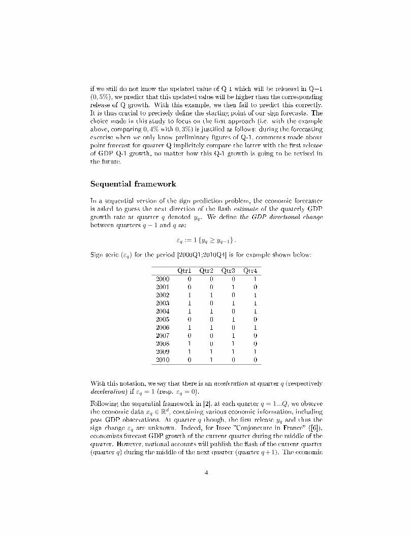
Sign serie (εq) for the period [2000Q1;2010Q4] is for example shown below:

Qtr1 Qtr2 Qtr3 Qtr42000 0 0 0 12001 0 0 1 02002 1 1 0 12003 1 0 1 12004 1 1 0 12005 0 0 1 02006 1 1 0 12007 0 0 1 02008 1 0 1 02009 1 1 1 12010 0 1 0 0

With this notation, we say that there is an acceleration at quarter q (respectivelydeceleration) if εq = 1 (resp. εq = 0).

Following the sequential framework in [2], at each quarter q = 1...Q, we observethe economic data xq ∈ Rd, containing various economic information, includingpast GDP observations. At quarter q though, the �rst release yq and thus thesign change εq are unknown. Indeed, for Insee �Conjoncture in France� ([6]),economists forecast GDP growth of the current quarter during the middle of thequarter. However, national accounts will publish the �ash of the current quarter(quarter q) during the middle of the next quarter (quarter q+1). The economic

4

forecaster is thus asked to guess the next outcome εq of a sequence of binaryoutcomes ({0, 1}) ε1, ..., εq−1with the knowledge of the past εq−1 := (ε1, ..., εq−1)and the side economic information xq := (x1, ..., xq): is there an acceleration ora deceleration? In other words, the elements ε1, ε1, ... and x1, x2, ...are revealedone at a time, beginning with (x1, y0), (x2, y1)...and the forecast at quarter q isbased on εq−1 and xq.

Formally, a forecasting strategy is de�ned as a family of predictors (φq)q:

εq := φq(xq, εq−1).

Business surveys

In this study, the economic information included in xq, apart from past GDPobservations, will be business surveys. Indeed, they are a useful source of infor-mation when forecasting, for they present three types of advantages: (1) theyprovide reliable information coming directly from the economic decision makers,(2) they are rapidly available (about a month after the questionnaires are sent),on a monthly, bimonthly or quarterly basis, and (3) they are subject to smallrevisions (each publication presents a generally negligible revision, only on thepreceding point). The disseminated statistics compiled from these surveys areusually balances of opinions. Recent economic information used in this studyto predict GDP growth sign incorporates Insee business surveys of all sectors(industry, services, wholesale trade, retail trade and building). Insee surveysamong business leaders are monthly qualitative surveys providing informationon the rate of activity in the recent past, during the current month and in thenear future. Industry survey for example questions 4,000 entrepreneurs aboutrecent and probable future trends in their production, about their total and for-eign order-book levels, inventory levels and general output prospects. Generally,these questions are qualitative: up, no change or down. The balance of opinion,de�ned as the di�erence between the percentage of positive responses and thepercentage of negative responses, is the most widely-used indicator by outlookanalysts to summarise answers to a question. Insee also publishes a compositeindicator called the french business climate indicator: it summarises informationthat is common to a set of 26 balances of opinion of all sectors business surveys([4]). Insee business surveys refering for month M are published during thesame month M . Hence they provide the best advanced indicator for the outputof the current quarter. Indeed, during our forecast exercise at the middle ofquarter Q, results of business surveys for the two �rst months of quarter Q areavailable. Quantitative indicators for month M (such as industrial productionindex,...) are most of the time not available before the end of month M + 1:they won't be taken into consideration here.

5

Loss function

To evaluate a forecasting strategy, we need to de�ne a loss function. At quarterq, the (normalized) cumulative loss related to the strategy (φq) is de�ned as:

Lq(φq) :=1q

q∑t=1

1(εt 6= εt).

This loss function is equivalent to the average error rate ηt := 1 {εt 6= εt} overthe period [1, q]. A natural loss function for risk adverse agents could makemisclassi�ed decelerations more costly than misclassi�ed accelerations. How-ever for sake of simplicity, we restrict our analysis to the symmetric indicatorloss. In the next sections, we compare forecasting errors for di�erent strategiessince 1997, date of the �rst available quarterly Insee GDP forecast. Indeed,we decided to compare the performance of the quantitative methods with Insee�Conjoncture in France� forecasts.

At this point, obviously, the mean error of any strategy takes its value in [0, 1].Lq(φq) = 0 (respectively Lq(φq) = 1 ) means that the strategy φq perfectly fore-casts the sequence of signs (resp. was wrong at all time). But in between, whatis a good strategy? In this study, our approach is to compare any strategy withthe optimal forecasting strategy of an uninformed forecaster trying to minimizehis loss. To minimize in probability the worst case over all possible outcomes,the uninformed agent forecast the next sign change by simply drawing a randomvariable from a Bernouilli with parameter 1/2.

εq = φrandomq (εq−1) = uq.

A simple model free test

The expected normalised loss is then ELq(φrandomq ) = 1/2, which means thaton the long run, the average error of a uninformed forecaster will be equal to0.5. Recall that qLq(φq) is distributed as a binomial distribution with param-eters n = q and p = 1/2. Thus, with great probability (95%) over the period[1997Q1;2010Q4] (52 quarters), the mean error is greater than 35%. A strategyis all the better than it is unlikely that an uninformed forecast reaches the sameerror rate. We de�ne the p-value of a strategy φq as

pq := P(Lq(φrandomq ) ≤ Lq(φq)).

By convention, we say that a strategy is signi�cant at level α if pq ≤ α. In otherwords, if pq ≤ α, it means that a random forecast has less than α% chances toget an error rate lower than the error rate Lq(φq) of the strategy φq.

6

3 Empirical comparison on historical data

In this section, we conduct a comparative study between di�erent class of mod-els ranging from econometrics to machine learning.. Our �rst benchmark corre-sponds to the quaterly forecasts released in Insee �Conjoncture in France� since1997. Our second class of benchmarks corresponds to �naive� strategies whenforecasters do not have any economic information except the serie of past direc-tions: εq−1. The results presented below show that the Insee strategie is a lotbetter than naive strategies.

3.1 Insee �Conjoncture in France� forecasts

Insee point forecasts are made from the observation of a wide set of French andinternational economic indicators (business surveys, quantitative indicators, �-nancial data...) combined with experts' judgement (related to, for example, theevolution of other developed countries activity, etc.). We de�ne Insee direction-nal forecast as:

εq = φInseeq := 1{yinseeq ≥ yq−1

}.

Insee mean error over the period [1997Q1;2010Q4] is around 20%. The corre-sponding p-value is 4, 0×10−6, which means that there is less than four chancesover a million that an uninformed forecaster could have outperformed the inseeforecasts. We consider now other naive strategies.

3.2 Naive strategies

Freeze strategy

Notice that, since 1997, quaterly signs (εq) have alternate about 63% of thetime. A strategy would be to predict, for each quarter, the opposite sign of theprevious observed direction change:

εq := φprev.valueq (εq−1) = 1− εq−1.

Numerical application: Freeze mean error over the period [1997Q1;2010Q4]is 36%. The corresponding p-value is 1, 8× 10−2.

Long term mean forecast

This strategy consists in assuming the current quarter sign to be equal to thelong term mean of the past observed signs (which is then rounded to 0 or 1).

7

εq = φlongtermq (εq−1) = 1

{1q

q∑t=1

εt ≥ 0, 5

}.

Numerical application: Long term strategy mean error is 41%. The corre-sponding p-value is 5, 0× 10−2.

Markov strategy

Here we assume εq to be the outcome of a homogeneous Markov chain of order1 with probability transition matrix Π. Forecast is then given by:

εq = φq(εq−1) := Argmaxi∈{0,1}Π(εq−1, i)

where Π(εq−1, i) := P(Eq = i|Eq−1 = εq−1).

In other words, suppose we observed at q−1 that εq−1 = j, then we will forecastfor quarter q the most likely occurrence of Eq when its previous value was j.

Numerical application: Markov strategy mean error since 1997 is 36%. Thecorresponding p-value is 1, 8× 10−2.

3.3 Business surveys based strategies

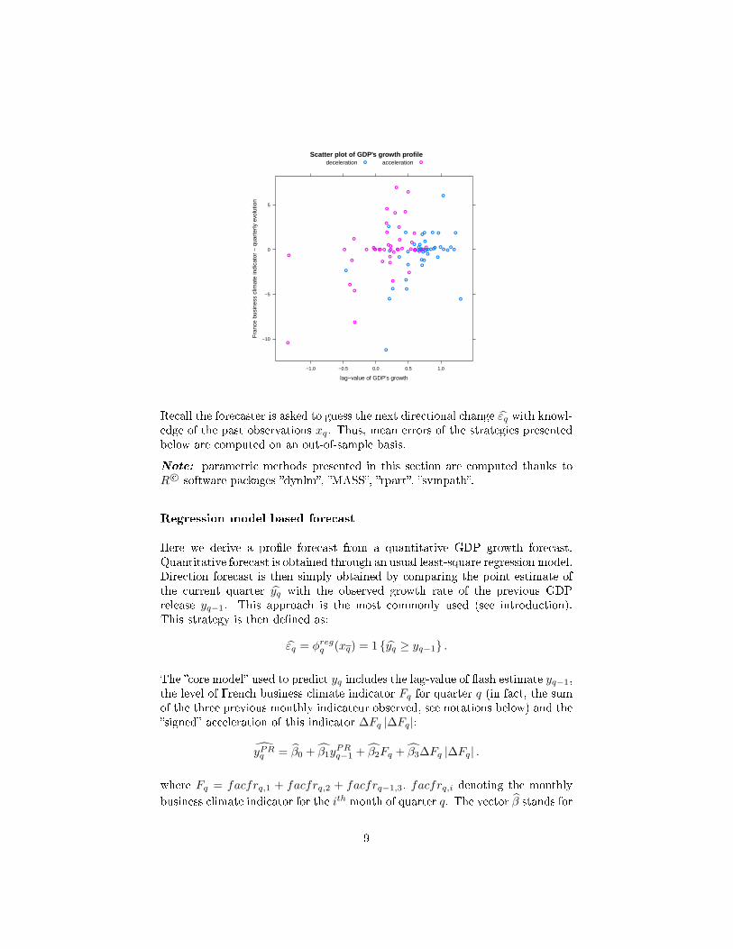
In this section, we incorporate business surveys in our strategies. Balances ofopinion from business surveys provide indeed an adequate predictor of the GDPsign change. For example, �gure below corresponds to GDP growth signs, withthe lag value of GDP's growth in the x-axis and the French business climategrowth in the y-axis. These two variables appear to be not-so-bad input vari-ables for sign prediction: activity is obviously more likely to accelerate whenbusiness climate is accelerating and when GDP growth during the previous quar-ter was low. This illustrates the opportunity to test parametric classi�cationmodels with business surveys as explanatory variables.

8

Scatter plot of GDP's growth profile

lag−value of GDP's growth

Fra

nce

busi

ness

clim

ate

indi

cato

r −

qua

rter

ly e

volu

tion

−10

−5

0

5

−1.0 −0.5 0.0 0.5 1.0

● ●● ●

●

●

● ●

●

●

●

●●

●

●

●

●

● ●

●

●

●

●

●

●●●

●

●

●

●

●

●●●

● ●●

●

●

●

●

●

●

●

●●●

●

●

● ●●

●

● ●

●

●

●

●

●

●

●●

●

●

●

●

●

●

●

●

●

● ●

●

●● ●

●●●

●●

●

●

●

●

●

●

deceleration acceleration● ●

Recall the forecaster is asked to guess the next directional change εq with knowl-edge of the past observations xq. Thus, mean errors of the strategies presentedbelow are computed on an out-of-sample basis.

Note: parametric methods presented in this section are computed thanks toR c© software packages �dynlm�, �MASS�, �rpart�, �svmpath�.

Regression model based forecast

Here we derive a pro�le forecast from a quantitative GDP growth forecast.Quantitative forecast is obtained through an usual least-square regression model.Direction forecast is then simply obtained by comparing the point estimate ofthe current quarter yq with the observed growth rate of the previous GDPrelease yq−1. This approach is the most commonly used (see introduction).This strategy is then de�ned as:

εq = φregq (xq) = 1 {yq ≥ yq−1} .

The �core model� used to predict yq includes the lag-value of �ash estimate yq−1,the level of French business climate indicator Fq for quarter q (in fact, the sumof the three previous monthly indicateur observed, see notations below) and the�signed� acceleration of this indicator ∆Fq |∆Fq|:

yPRq = β0 + β1yPRq−1 + β2Fq + β3∆Fq |∆Fq| .

where Fq = facfrq,1 + facfrq,2 + facfrq−1,3, facfrq,i denoting the monthlybusiness climate indicator for the ith month of quarter q. The vector β stands for

9

the ordinary least square estimates. Recall that during the forecasting exercisearound the middle of quarter q, the most recent availabe indicator is facfrq,2.

Numerical application: The normalised loss of the regression based strategyεq = 1 {yq ≥ yq−1} is 18% since 1997. The corresponding p-value is 8, 4× 10−7.

We also estimate a second model, which includes balances of opinion in manu-facturing industry dealing with recent changes in output (manuf.tppaq,i) andpersonal production expectations (manuf.tppreq,i). Output in manufacturingindustry is indeed considered as one of the best leading input variables for GDPgrowth:

yq = β0 + β1yq−1 + β2yq−4 + β3manuf.tppaq,2 + β4(manuf.tppaq,2 −manuf.tppaq,1)

+β5(manuf.tppreq,2 −manuf.tppreq,1) + β6 (manuf.tppreq,1 −manuf.tppreq−1,3).

Numerical application: Sign mean error with the pro�le based on the �man-ufacturing model� is 18%. The corresponding p-value is 8, 4× 10−7.

Probit forecast

Signs εq can be directly predicted through a parametric probit model, with aset of explanatory variables xq. This model states that:

P (εq = 1|Xq = xq) = F (βxq)

where F is the cumulative normal distribution. Coe�cients β are estimated bylikelihood maximisation. Sign forecasts are then given by:

εq = φprobq (xq, εq−1) = 1{F (βxq) ≥ 0, 5

}.

Here we also consider two sets of variables for xq :

• the �core� variables used in the �core model� of the previous section

(yq−1,∆Fq,∆Fq |∆Fq|).

• the �manufacturing� variables used in the �manufacturing model� of theprevious section(

yq−1, yq−4,manuf.tppaq,2,manuf.tppaq,2 −manuf.tppaq,1,manuf.tppreq,2 −manuf.tppreq,1,manuf.tppreq,1 −manuf.tppreq−1,3

)

Numerical application : The mean loss for �core� model (resp. manufacturingmodel) is 14% (resp. 16%) since 1997. The corresponding p-value is 3, 6× 10−8.

10

�Linear/Quadratic discriminant analysis� (LDA/QDA)

Linear discriminant analysis (LDA) is a classi�cation method. It provides lineardecision boundaries depending on the observed variables Xq (for more detailssee [8] and references therein). This method requires the knowledge of the classposteriors Pr(ε/X = .). Let fk(.) be the posterior density of X given class ε = k

(k ∈ (0, 1)), and let πk be the prior probability of class k, with∑1k=0 πk = 1 .

A simple application of Bayes theorem gives us :

Pr(ε = k|X = x) =fk(x)πk∑1l=0 fl(x)πl

.

Suppose each class density fk(x) is a multivariate Gaussian with mean µk andcovariance matrix Σk. Linear discriminant analysis arises in the special casewhen we assume that the classes have a common covariance matrix Σk = Σ ∀k(otherwise we apply the term �quadratic discriminant analysis� - QDA - wheremore factors are to be estimated). In practice, the parameters (πk,µk,Σk) areunknown, so we must estimate them through our historical data :

• πk = Nk/N , where Nk is the number of class-k observations,

• µk =∑εq=k

xq/Nk ;

• Σ =∑εq=k

(xq − µk)(xq − µk)T /(N −K).

The LDA rules can be written as a function of these estimated parameters. Moreprecisely, the LDA rule classi�es the observations xq in class k = 1 rather thanclass k = 0 if :

Pr(εq = 1|Xq = xq) > Pr(εq = 0|Xq = xq)

⇐⇒ xT Σ−1(µ1 − µ0) > 12µ1

T Σ−1µ1 − 12µ0

T Σ−1µ0 + log(N0/N)− log(N1/N).

We see that decision boundaries correspond to linear functions of the explana-tory variables xq. Pro�le forecast is then given by :

εq = φLDAq (xq) = 1

{xT

q Σ−1(µ1 − µ0) >1

2µ1

T Σ−1µ1 −1

2µ0

T Σ−1µ0 + log(N0/N)− log(N1/N)

}.

Notice that with two classes there is a simple correspondence between LDA andclassi�cation by linear least squares. This is equivalent to directly estimate themodel δq = β0 +β1y

PRq−1 +β2Fq+β3∆Fq |∆Fq|+ξq, then to classify εq according

to the position of δq compared to 0.5.

Numerical application : We consider for Xq the �core variables� presentedabove. Mean of forecasting errors is 12% since 1997. The corresponding p-valueis 6, 5× 10−9.

We also considered the LDA-extension method, i.e. the quadratic discriminantanalysis (QDA). The mean loss is a bit higher than with the LDA method (14%

11

since 1997). Indeed, QDA implies the estimation of a lot more parameters (thevariance parameters, see above) than LDA, with a limited number of observa-tions (around 76 quarterly observations in our case). Consequently, due to anincreasing complexity, results are then less accurate.

Recursing partitioning (RPART)

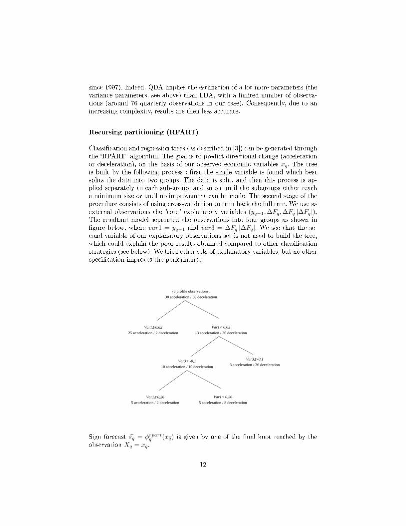
Classi�cation and regression trees (as described in [3]) can be generated throughthe �RPART� algorithm. The goal is to predict directional change (accelerationor deceleration), on the basis of our observed economic variables xq. The treeis built by the following process : �rst the single variable is found which bestsplits the data into two groups. The data is split, and then this process is ap-plied separately to each sub-group, and so on until the subgroups either reacha minimum size or until no improvement can be made. The second stage of theprocedure consists of using cross-validation to trim back the full tree. We use asexternal observations the �core� explanatory variables (yq−1,∆Fq,∆Fq |∆Fq|).The resultant model separated the observations into four groups as shown in�gure below, where var1 = yq−1 and var3 = ∆Fq |∆Fq|. We see that the se-cond variable of our explanatory observations set is not used to build the tree,which could explain the poor results obtained compared to other classi�cationstrategies (see below). We tried other sets of explanatory variables, but no otherspeci�cation improves the performance.

78 profile observations :

38 acceleration / 38 deceleration

Var1≥ 0,62


Var1< 0,62


Var3< -0,1


Var3≥ -0,1


Var1≥ 0,26


Var1< 0,26


Sign forecast εq = φrpartq (xq) is given by one of the �nal knot reached by theobservation Xq = xq.

12

Numerical application : The mean error since 1997 is 25%. The correspon-ding p-value is 9, 1× 10−5.

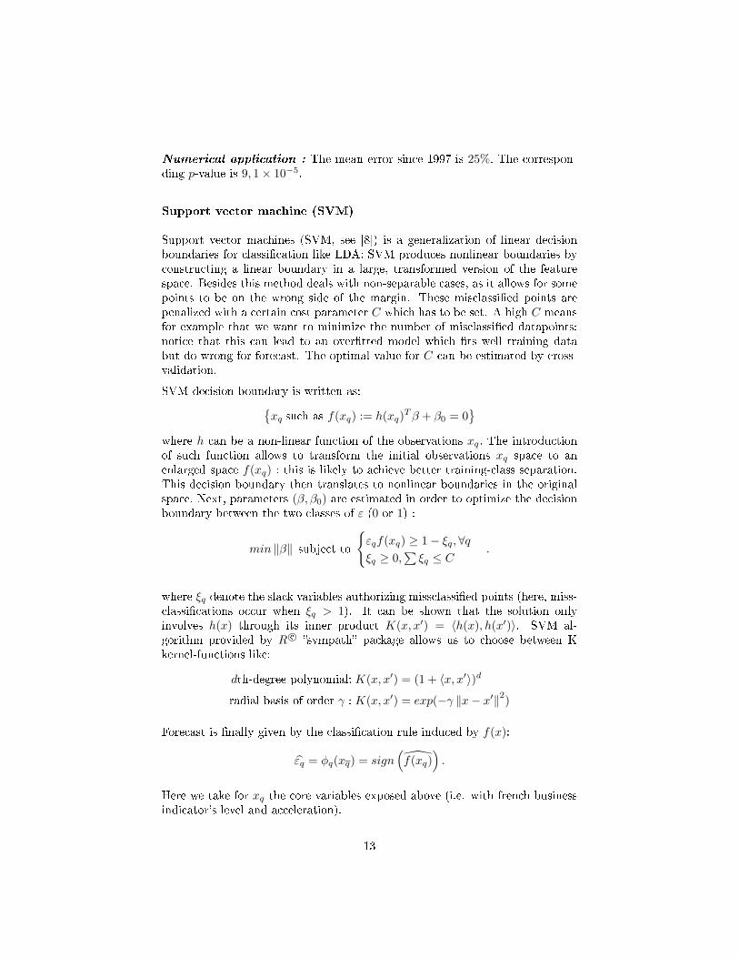
Support vector machine (SVM)

Support vector machines (SVM, see [8]) is a generalization of linear decisionboundaries for classi�cation like LDA: SVM produces nonlinear boundaries byconstructing a linear boundary in a large, transformed version of the featurespace. Besides this method deals with non-separable cases, as it allows for somepoints to be on the wrong side of the margin. These misclassi�ed points arepenalized with a certain cost parameter C which has to be set. A high C meansfor example that we want to minimize the number of misclassi�ed datapoints:notice that this can lead to an over�tted model which �ts well training databut do wrong for forecast. The optimal value for C can be estimated by cross-validation.

SVM decision boundary is written as:{xq such as f(xq) := h(xq)Tβ + β0 = 0

}where h can be a non-linear function of the observations xq. The introductionof such function allows to transform the initial observations xq space to anenlarged space f(xq) : this is likely to achieve better training-class separation.This decision boundary then translates to nonlinear boundaries in the originalspace. Next, parameters (β, β0) are estimated in order to optimize the decisionboundary between the two classes of ε (0 or 1) :

min ‖β‖ subject to

{εqf(xq) ≥ 1− ξq,∀qξq ≥ 0,

∑ξq ≤ C

.

where ξq denote the slack variables authorizing missclassi�ed points (here, miss-classi�cations occur when ξq > 1). It can be shown that the solution onlyinvolves h(x) through its inner product K(x, x′) = 〈h(x), h(x′)〉. SVM al-gorithm provided by R c© �svmpath� package allows us to choose between Kkernel-functions like:

dth-degree polynomial: K(x, x′) = (1 + 〈x, x′〉)d

radial basis of order γ : K(x, x′) = exp(−γ ‖x− x′‖2)

Forecast is �nally given by the classi�cation rule induced by f(x):

εq = φq(xq) = sign(f(xq)

).

Here we take for xq the core variables exposed above (i.e. with french businessindicator's level and acceleration).

13

Out-of-sample forecast errors are fewer when we set a high cost parameter C (i.e.when we are close to a separable case). Hence we see here that there is no gainin enlarging our observation space with a non-linear function h. Besides, kernel-function K that leads to the best out-of-sample performance is the 1th-degreepolynomial function: this is equivalent to a linear decision boundary.

Numerical application:The error rate is then 16% since 1997. The corre-sponding p-value is 1, 8× 10−7.

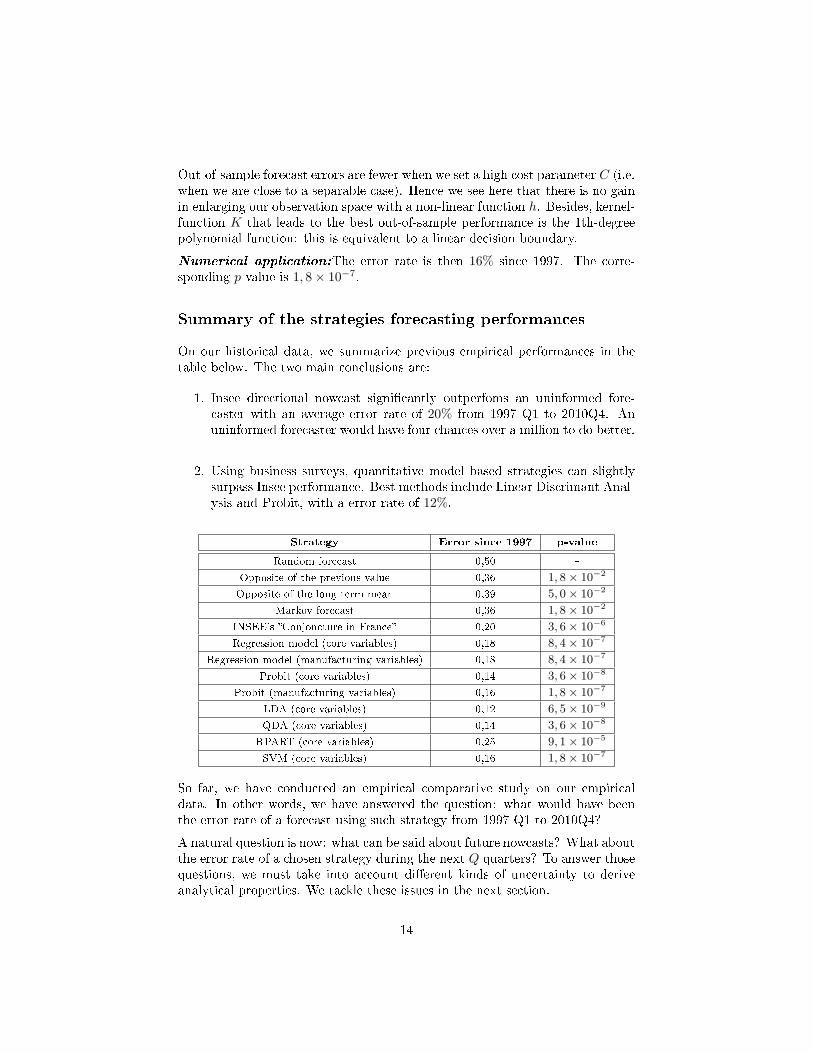
Summary of the strategies forecasting performances

On our historical data, we summarize previous empirical performances in thetable below. The two main conclusions are:

1. Insee directional nowcast signi�cantly outperfoms an uninformed fore-caster with an average error rate of 20% from 1997 Q1 to 2010Q4. Anuninformed forecaster would have four chances over a million to do better.

2. Using business surveys, quantitative model based strategies can slightlysurpass Insee performance. Best methods include Linear Discrimant Anal-ysis and Probit, with a error rate of 12%.

Strategy Error since 1997 p-value

Random forecast 0,50 -Opposite of the previous value 0,36 1, 8× 10−2

Opposite of the long-term mean 0,39 5, 0× 10−2

Markov forecast 0,36 1, 8× 10−2

INSEE's �Conjoncture in France� 0,20 3, 6× 10−6

Regression model (core variables) 0,18 8, 4× 10−7

Regression model (manufacturing variables) 0,18 8, 4× 10−7

Probit (core variables) 0,14 3, 6× 10−8

Probit (manufacturing variables) 0,16 1, 8× 10−7

LDA (core variables) 0,12 6, 5× 10−9

QDA (core variables) 0,14 3, 6× 10−8

RPART (core variables) 0,25 9, 1× 10−5

SVM (core variables) 0,16 1, 8× 10−7

So far, we have conducted an empirical comparative study on our empiricaldata. In other words, we have answered the question: what would have beenthe error rate of a forecast using such strategy from 1997 Q1 to 2010Q4?

A natural question is now: what can be said about future nowcasts? What aboutthe error rate of a chosen strategy during the next Q quarters? To answer thosequestions, we must take into account di�erent kinds of uncertainty to deriveanalytical properties. We tackle these issues in the next section.

14

4 Prediction for future sign forecasts

4.1 Test of independence

Recall the forecast errors are denoted by ηt := 1 {εt 6= εt}. To model uncer-tainty, we consider (ηq) as the outcome of a random process (Hq). In orderto derive analytical properties, a central point is then to test whether forecasterrors are independent or not. For example, if forecast errors of a given strategyare concentrated over the end of the period, it will raise serious doubts aboutthe ability of this strategy to predict next GDP growth signs. Non stationaryunderlying processes could for instance explain such time-correlated forecast er-rors. For the sake of simplicity, we suppose that the time dependency can be oforder 1 at the most. Recall that independence is equivalent to: for any t, i, j,

P(Ht = i,Ht−1 = j) = P(Ht = i)P(Ht−1 = j)

which can be rewritten as:

P(Ht = 1, Ht−1 = 1) = P(Ht = 1)P(Ht−1 = 1)P(Ht = 1, Ht−1 = 0) = P(Ht = 1)P(Ht−1 = 0)P(Ht = 0, Ht−1 = 1) = P(Ht = 0)P(Ht−1 = 1)P(Ht = 0, Ht−1 = 0) = P(Ht = 0)P(Ht−1 = 0)

.

Since (ηt) is a dummy function, previous equations are equivalent to test thesingle equation Cov(Ht, Ht−1) = 0.

Proposition 1 With the previous asumptions, an asymptotic α-level test forthe null hypothesis H0 := {Cov(Ht, Ht−1) = 0} can be de�ned by the followingreject region: {∣∣∣∣∣

√QCov(Ht, Ht−1)√

λ′Σλ

∣∣∣∣∣ > q1−α/2

}.

with λ := (1, E(Z3t ), E(Z2

t ))′, Zi :=

Hi−1Hi

Hi

Hi−1

, and Σ := V ar(Z1) +

2 [cov(Z1, Z2) + cov(Z1, Z3)] and q1−α/2 the 1− α/2 normal quantile.

Proof: see appendices.

Numerical application: For all the strategies presented above, we do notreject the null hypothesis of independent forecast errors. Indeed relevant testsall belong to [−1.2, 0.5], that is inside the 95% con�dence interval [−1.96, 1.96].As a conclusion, we will assume afterwards that forecast errors of all strategiesare time-independent. However, two di�erent strategies can still have correlatedforecast errors.

15

4.2 What is the future error rate of a given strategy ?

Asymptotic approach

For a given strategy φ1, we estimated the mean of forecast errors with thehistorical data by p1. We now want to predict the mean of the future forecasterrors during the next h quarters ηq, q = Q+ 1...Q+ h. The mean of the futureforecast errors during the next h quarters will be 1

h

∑Q+ht=Q+1 ηt.

If h is large enough, we apply the central limit theorem and we have asympto-tically with probability 1− α :

1h

Q+h∑t=Q+1

Ht ∈ p1 ±σq1−α/2√

h

with p1 the (unobserved) true expected error rate for strategy φ1, σ is the(unobserved) stantard-deviation of ηt, and q1−α is the (1 − α)-quantile of thestandard normal distribution. Thus, the length of the con�dence interval iscontroled by a forescast error which converges to 0 at rate 1/

√h. However, since

p1 is unknown, we must estimate it through our historical dataset. Denoting Qthe size of our historical sample, we obtain for large Q with probability 1− α :

p1 ∈ p1 ±σq1−α/2√

Q.

In this equation, the length of the con�dence interval is controlled by an esti-mation error term which tends to 0 at rate 1/

√Q. Combining both equations,

and replacing σ by its empirical counterpart σ :=√

1Q−1

∑Qq=1(Hq − H)2 =√

p1(1− p1), we apply the central limit theorem for large Q and h.

Proposition 2 Under previous asumptions, we get asymptotically with proba-bility 1− α :

1Q

Q∑t=1

Ht ∈ p1 ± σq1−α/4

1√h︸︷︷︸

Forecast error

+1√Q︸︷︷︸

Estimation error

.Thus, uncertainty, measured as the length of the con�dence interval, results fromtwo sources of uncertainty : forecast uncertainty and estimation uncertainty.

Numerical application : with p1 ≈ 0, 15 (e.g. a value close to our best stra-tegies), we obtain :

• with N = 60 (15 years) and Q = 8 (2 years) the 90% con�dence intervalfor the future mean of forecasts errors will be [0, 0.5].

16

• with N = 60 (15 years) and Q = 60 (15 years) the 90% con�dence intervalfor the future mean of forecasts errors will be[0, 0.33].

These con�dence intervals for future forecasts may look quite large. But noticethat any of our parametric strategies is a lot more successful than the randomstrategy. The upper bound of the relevant 90% con�dence interval for best pa-rametric strategies (e.g. around 0.5 with N = 60 and Q = 8) is indeed around0.5 with N = 60 and Q = 8. At the same time, an uninformed agent will only beable to give the following con�dence interval for the mean of its future forecasterrors : 0.5± 0.5 ∗ 2 ∗ (1/

√60 + 1/

√8) = [0.1]. The corresponding upper bound

hence reaches in that case the maximum possible value of 1 !

Finite sample approach

Previous results are only valid when Q and h are large (application of the centrallimit theorem). However, in practice, we only have access to a limited numberof observations. Thus the relevance of previous bounds can be challenged. Inthis paragraph, we derive �nite sample results to deal with this issue.

A �rst approach consists in using Hoe�ding's inequality ([10]). The latter up-perbounds the probability that the distance between empirical mean and ex-pectation is large.

Proposition 3 Then, with a probability lower than 1− α, we have :

| 1Q

∑q

Hq − p1| ≤√

ln(4/α)2

(1√Q

+1√N

).

Proof : see appendices.

Numerical application : for N = 60 and Q = 8 the interval length aroundp1 is ±0, 6 ! (±0, 3 when N = Q = 60).

We lose a precision factor of order 3 in these bounds in comparison with theasymptotic approach. If we compare the two expressions, the variance term σ ismissing in the �nite sample bounds. Thus it is a uniform bound that does nottake into account the fact that the variance can be small. To �ll the gap, usinginequality in [11], we derive an upper bound with an empirical variance term.

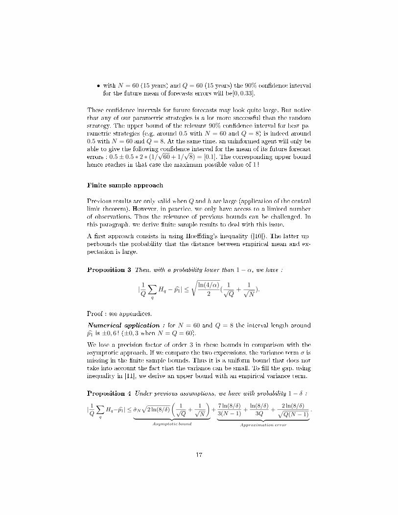
Proposition 4 Under previous assumptions, we have with probability 1− δ :

| 1Q

∑q

Hq−p1| ≤ σN

√2 ln(8/δ)

(1√Q

+1√N

)︸︷︷︸

Asymptotic bound

+7 ln(8/δ)

3(N − 1)+

ln(8/δ)

3Q+

2 ln(8/δ)√Q(N − 1)︸︷︷︸

Approximation error

.

17

Proof : see appendices.

The con�dence interval length is of order ±0, 5 (h = Q = 60). This disap-pointing result in comparison with the previous inequality is due to the factthat, in our case, the empirical variance σN is not small enough to compensatethe approximation term. However it still might be interesting for other appli-cations. As expected, the length of the con�dence interval is larger in the �nitesample approach than in the asymptotic framework. Thus, for practical pur-poses, economic forecasters may consider those intervals too large. To deal withthis issue, notice that the error rate can be seen as an average error over allpossible outcomes xq. In probability terms, the empirical error rate estimatesthe unconditionnal expected error i.e. EXq,εq (εq). For a particular quarter q, itis all the more interesting for the forecaster to give a conditionnal directionalscenario, i.e. E(εq|Xq = xq). Indeed, if on average, the error rate is equal to12%, the conditional error E(εq|Xq = xq) could be even smaller. This partialconclusion advocates for a conditional approach.

5 Directional risk index

In this section, we de�ne a �directional risk index�, which will give for eachquarter the conditional probability of success (or failure) associated with ourdirectional forecast. More precisely, it will give the probability to be in an acce-leration state (e.g. εq = 1) or in a deceleration state (e.g. εq = 0). For symmetryreason, this �pro�le index� ranges from −1 (deceleration) to +1 (acceleration).We de�ne the directional risk index by :

Iq := 2(P(εq = +1|xq)− 1/2)

with P(εq = +1|xq) the estimated conditional probability of being in an acce-leration state given the knowledge of the business surveys up to quarter q. Wecan also de�ne an �area of uncertainty� when, by convention, the directional riskindex lies in the interval [−0.5,+0.5]. A pro�le forecast associated with a direc-tional risk index that falls into the area of uncertainty has then to be consideredcarefully. To build this probability index, we consider two previous strategies :the regression model strategy, and the probit strategy.

5.1 Directional risk index derived from the regression me-

thod

To derive such an index, we need somehow to introduce probability in the pre-vious strategy. In the regression approach, it is usual to assume a linear statis-tical model with i.i.d. errors such that :

yq = β0 + β1yq−1 + β2Fq + β3∆Fq |∆Fq|+ ξq

18

This model gives for each quarter q the growth level forecast yq. Recall signforecast was then given by :

φq(xq) = 1 {yq ≥ yq−1}

with yq = x′

qβ and β the ordinary least square estimate. We estimate the densityof the error term ξq with a kernel-type estimation :

fξ(x) =1Nh

Q∑q=1

K(x− xqh

)

where h is the optimal kernel bandwidth. It follows that :

Pq(εq = 1) = Pq(ξq ≥ yq−1 − x′

qβ) ≈ Pfξ(ξq ≥ yq−1 − x′

qβ)

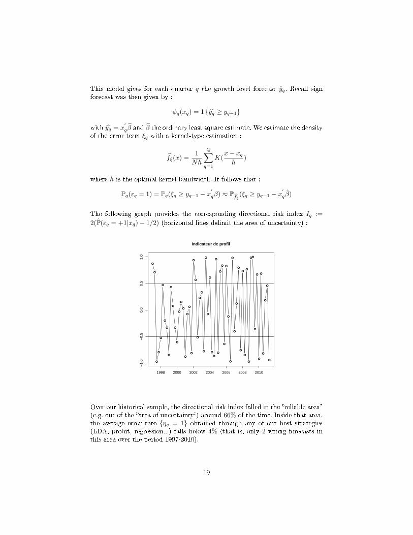
The following graph provides the corresponding directional risk index Iq :=2(P(εq = +1|xq)− 1/2) (horizontal lines delimit the area of uncertainty) :

●

●

●

●

●

●

●

●

●

●

●

●

●

●

●

●

●

●

●

●

●

●

●

●

●

●

●

●

●

●

●

●

●

●

●

●

●

●

●

●

●

●

●

●

●

●

●

●

●●

●

●

●

●

●

●

●

●

Indicateur de profil

1998 2000 2002 2004 2006 2008 2010

−1.

0−

0.5

0.0

0.5

1.0

Over our historical sample, the directional risk index falled in the �reliable area�(e.g. out of the �area of uncertainty�) around 66% of the time. Inside that area,the average error rate {ηq = 1} obtained through any of our best strategies(LDA, probit, regression...) falls below 4% (that is, only 2 wrong forecasts inthis area over the period 1997-2010).

19

5.2 Directional risk index derived from the probit strategy

Recall the assumptions behind our probit forecast strategy :

P(εq = 1|Xq = xq) = F (βxq)

With our previous notations, we can then easily de�ne our directional risk indexas :

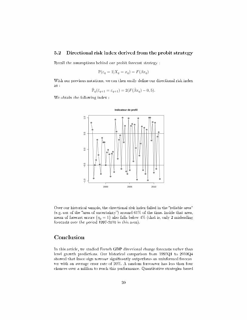
Pq(εq+1 = εq+1) = 2(F (βxq)− 0, 5).

We obtain the following index :

●

●

●

●

●

●

●

●

●

●

●●

●

●

●

●

●

●

●

●

●

●

●

●

●

●

●

●

●

●

●

●

●

●

●

●

●

●

●

●

●

●

●

●

●

●

●

●

●●

●

●

●

●

●

●

●

●

Indicateur de profil

2000 2005 2010

−1.

0−

0.5

0.0

0.5

1.0

Over our historical sample, the directional risk index falled in the �reliable area�(e.g. out of the �area of uncertainty�) around 61% of the time. Inside that area,mean of forecast errors {ηq = 1} also falls below 4% (that is, only 2 misleadingforecasts over the period 1997-2010 in this area).

Conclusion

In this article, we studied French GDP directional change forecasts rather thanlevel growth predictions. Our historical comparison from 1997Q1 to 2010Q4showed that Insee sign nowcast signi�cantly outperfoms an uninformed forecas-ter with an average error rate of 20%. A random forecaster has less than fourchances over a million to reach this performance. Quantitative strategies based

20

on business surveys such as Linear Discrimant Analysis can slightly surpass In-see performance, with an error rate of 12%. Eventually, using our directionalrisk index, an economic forecaster can even specify the uncertainty inherent tohis directional forecast and conditional on present economic information.

Références

[1] M. Bessec. Etalonnages du taux de croissance du pib français sur la basedes enquêtes de conjoncture. Economie & prévision, (2) :77�99, 2010.

[2] G. Biau, K. Bleakley, L. Györ�, and G. Ottucsák. Nonparametric sequentialprediction of time series. Journal of Nonparametric Statistics, 22(3) :297�317, 2010.

[3] L. Breiman. Classi�cation and regression trees. Chapman & Hall/CRC,1984.

[4] L. Clavel and C. Minodier. A monthly indicator of the french businessclimate. Documents de Travail de la DESE-Working Papers of the DESE,2009.

[5] É. Dubois and E. Michaux. Étalonnages à l'aide d'enquêtes de conjoncture :de nouveaux résultats. Economie & prévision, (1) :11�28, 2006.

[6] S. Duchêne and JF Ouvrard. La prevision des comptes de la zone euro àpartir des enquêtes de conjoncture. Note de Conjoncture (mars), INSEE,2011.

[7] H. Erkel-Rousse and C. Minodier. Do business tendency surveys in industryand services help in forecasting GDP growth ? A real-time analysis on frenchdata. Documents de Travail de la DESE-Working Papers of the DESE,INSEE, 2009.

[8] T. Hastie, R. Tibshirani, and J.H. Friedman. The elements of statisticallearning : data mining, inference, and prediction. Springer Verlag, 2009.

[9] R.D. Henriksson and R.C. Merton. On market timing and investmentperformance. II. Statistical procedures for evaluating forecasting skills. TheJournal of Business, 54(4) :513�533, 1981.

[10] W. Hoe�ding. Probability inequalities for sums of bounded random va-riables. Journal of the American Statistical Association, 58(301) :13�30,1963.

[11] A. Maurer and M. Pontil. Empirical bernstein bounds and sample variancepenalization. Arxiv preprint, 2009.

21

[12] R.C. Merton. On market timing and investment performance. I. An equi-librium theory of value for market forecasts. The Journal of Business,54(3) :363�406, 1981.

[13] G.H. Moore. Forecasting short-term economic change, 1983.

[14] M.H. Pesaran and A. Timmermann. A simple nonparametric test of predic-tive performance. Journal of Business & Economic Statistics, 10(4) :461�465, 1992.

[15] M.H. Schnader and H.O. Stekler. Evaluating predictions of change. TheJournal of Business, 63(1) :99�107, 1990.

[16] F. Sedillot and N. Pain. Indicator models of real GDP growth in selectedOECD countries. OECD Economics Department Working Papers, 2003.

[17] T.M. Sinclair, HO Stekler, and L. Kitzinger. Directional forecasts of GDPand in�ation : a joint evaluation with an application to Federal Reservepredictions. Applied Economics, 42(18) :2289�2297, 2010.

[18] H.O. Stekler. Are economic forecasts valuable ? Journal of Forecasting,13(6) :495�505, 1994.

[19] K.F. Wallis. Macroeconomic forecasting : a survey. The Economic Journal,99(394) :28�61, 1989.

22

Appendices

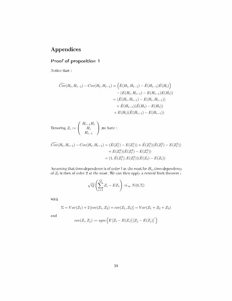
Proof of proposition 1

Notice that :

Cov(Ht, Ht−1)− Cov(Ht, Ht−1) =(E(Ht, Ht−1)− E(Ht−1)E(Ht)

)− (E(Ht, Ht−1)− E(Ht−1)E(Ht))

= (E(Ht, Ht−1)− E(Ht, Ht−1))

+ E(Ht−1)(E(Ht)− E(Ht))

+ E(Ht)(E(Ht−1)− E(Ht−1))

Denoting Zi :=

Hi−1Hi

Hi

Hi−1

,we have :

Cov(Ht, Ht−1)− Cov(Ht, Ht−1) = (E(Z1t )− E(Z1

t )) + E(Z3t )(E(Z2

t )− E(Z2t ))

+ E(Z2t )(E(Z3

t )− E(Z3t ))

= (1, E(Z3t ), E(Z2

t ))(E(Zt)− E(Zt))

Assuming that time-dependence is of order 1 at the most forHt, time-dependencyof Zt is then of order 2 at the most. We can then apply a central limit theorem :

√Q

(Q∑i=1

Zi − EZ1

)⇒∞ N(0,Σ)

with

Σ = V ar(Z1) + 2 [cov(Z1, Z2) + cov(Z1, Z3)] = V ar(Z1 + Z2 + Z3)

andcov(Zi, Zj) := sym

(E [Zi − E(Zi)] [Zj − E(Zj)]

′)

23

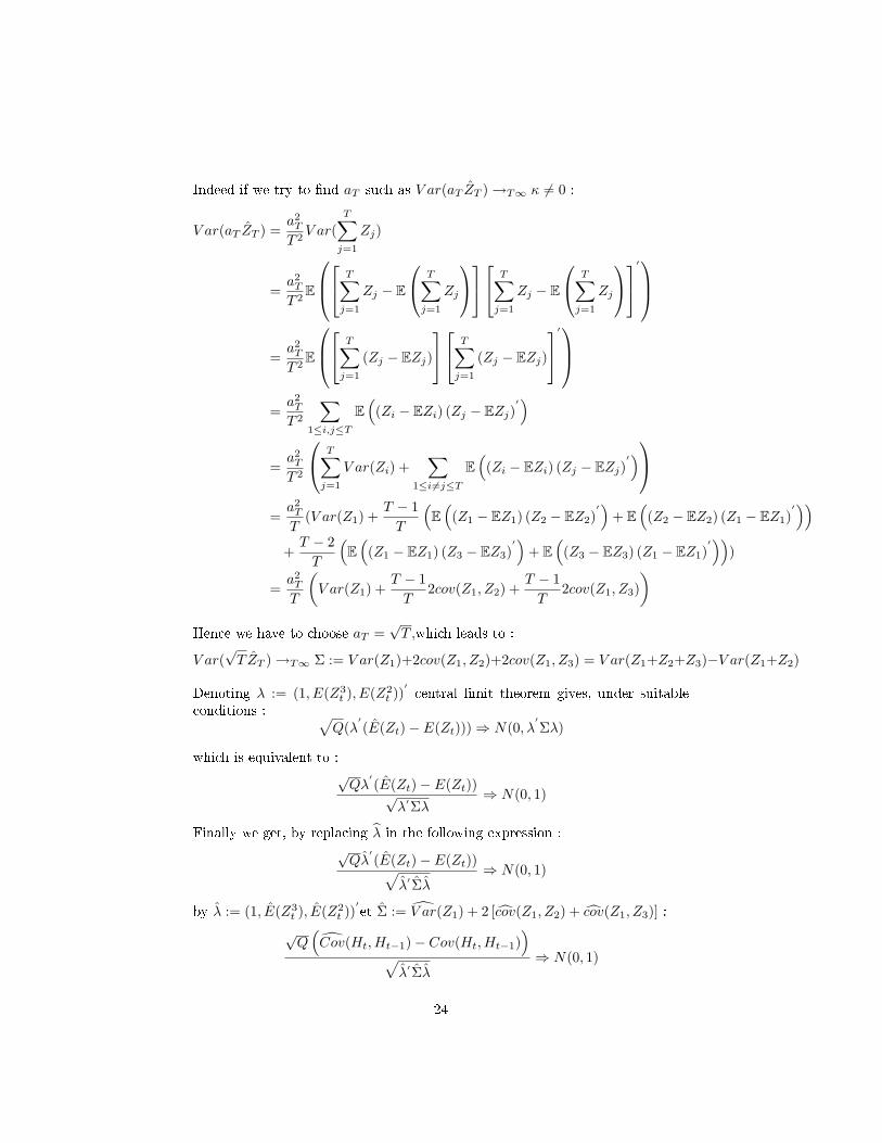
Indeed if we try to �nd aT such as V ar(aT ZT )→T∞ κ 6= 0 :

V ar(aT ZT ) =a2T

T 2V ar(

T∑j=1

Zj)

=a2T

T 2E

T∑j=1

Zj − E

T∑j=1

Zj

T∑j=1

Zj − E

T∑j=1

Zj

′

=a2T

T 2E

T∑j=1

(Zj − EZj)

T∑j=1

(Zj − EZj)

′

=a2T

T 2

∑1≤i,j≤T

E(

(Zi − EZi) (Zj − EZj)′)

=a2T

T 2

T∑j=1

V ar(Zi) +∑

1≤i6=j≤T

E(

(Zi − EZi) (Zj − EZj)′)

=a2T

T(V ar(Z1) +

T − 1T

(E(

(Z1 − EZ1) (Z2 − EZ2)′)

+ E(

(Z2 − EZ2) (Z1 − EZ1)′))

+T − 2T

(E(

(Z1 − EZ1) (Z3 − EZ3)′)

+ E(

(Z3 − EZ3) (Z1 − EZ1)′))

)

=a2T

T

(V ar(Z1) +

T − 1T

2cov(Z1, Z2) +T − 1T

2cov(Z1, Z3))

Hence we have to choose aT =√T ,which leads to :

V ar(√T ZT )→T∞ Σ := V ar(Z1)+2cov(Z1, Z2)+2cov(Z1, Z3) = V ar(Z1+Z2+Z3)−V ar(Z1+Z2)

Denoting λ := (1, E(Z3t ), E(Z2

t ))′central limit theorem gives, under suitable

conditions : √Q(λ

′(E(Zt)− E(Zt)))⇒ N(0, λ

′Σλ)

which is equivalent to :√Qλ

′(E(Zt)− E(Zt))√

λ′Σλ⇒ N(0, 1)

Finally we get, by replacing λ in the following expression :√Qλ

′(E(Zt)− E(Zt))√

λ′Σλ⇒ N(0, 1)

by λ := (1, E(Z3t ), E(Z2

t ))′et Σ := V ar(Z1) + 2 [cov(Z1, Z2) + cov(Z1, Z3)] :

√Q(Cov(Ht, Ht−1)− Cov(Ht, Ht−1)

)√λ′Σλ

⇒ N(0, 1)

24

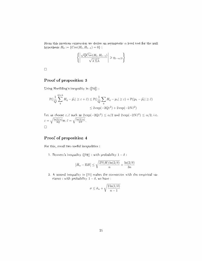
From this previous expression we derive an asymptotic α-level test for the nullhypothesis H0 := {Cov(Ht, Ht−1) = 0} :{∣∣∣∣∣

√QCov(Ht, Ht−1)√

λ′Σλ

∣∣∣∣∣ > q1−α/2

}

�


Using Hoe�ding's inequality in ([10]) :

P(| 1Q

Q+h∑q

Hq − p1| ≥ ε+ ε) ≤ P(| 1Q

∑q

Hq − p1| ≥ ε) + P(|p1 − p1| ≥ ε)

≤ 2 exp(−2Qε2) + 2 exp(−2Nε2)

Let us choose ε, ε such as 2 exp(−2Qε2) ≤ α/2 and 2 exp(−2Nε2) ≤ α/2, i.e.

ε =√

ln(2/α)2Q et ε =

√ln(2/α)

2N .

�


For this, recall two useful inequalities :

1. Bennett's inequality ([10]) : with probability 1− δ :

∣∣Hn − EH∣∣ ≤√2V(H) ln(2/δ)

n+

ln(2/δ)3n

2. A second inequality in [11] makes the connection with the empirical va-riance : with probability 1− δ, we have :

σ ≤ σn +

√2 ln(1/δ)n− 1

25

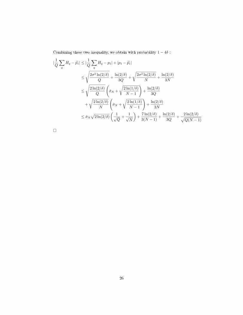
Combining these two inequality, we obtain with probability 1− 4δ :

| 1Q

∑q

Hq − p1| ≤ |1Q

∑q

Hq − p1|+ |p1 − p1|

≤

√2σ2 ln(2/δ)

Q+

ln(2/δ)3Q

+

√2σ2 ln(2/δ)

N+

ln(2/δ)3N

≤

√2 ln(2/δ)

Q

(σN +

√2 ln(1/δ)N − 1

)+

ln(2/δ)3Q

+

√2 ln(2/δ)

N

(σN +

√2 ln(1/δ)N − 1

)+

ln(2/δ)3N

≤ σN√

2 ln(2/δ)(

1√Q

+1√N

)+

7 ln(2/δ)3(N − 1)

+ln(2/δ)

3Q+

2 ln(2/δ)√Q(N − 1)

�

26