“Nowcasting”   County   Unemployment   Using   Twitter   Data 

Megha   Srivastava Thao   Nguyen Department   of   Computer   Science Department   of   Computer   Science 

Undergraduate   Student Undergraduate   Student 

Stanford   University Stanford   University 

Stanford,   CA   94305 Stanford,   CA   94305 

meghas@stanford.edu thao2605@stanford.edu   

Abstract 

Unemployment has negative effects on both the financial and mental health of the unemployed.                           

Social media and web searches can provide valuable insights into national unemployment                       

conditions. However, non­profit organizations and policy­makers combatting local unemployment                 

must rely on less timely county­level statistics. We combine geo­located Twitter data with data                           

from the Bureau of Labor Statistics to “nowcast” (predict the present) unemployment rate and                           

mass layoff events. Because relatively few tweets in a county­month discuss unemployment                       

directly, we use deep learning techniques to uncover hidden relationships between tweet content                         

and local unemployment conditions. We compare different deep learning models and parameters,                       

and   achieve   a   root   mean   square   value   of   1.08   on   our   best   performing   model. 

1 Introduction Although current access and use of information analyzing unemployment rates in the United States typically occurs                               

on the national level, the emotional and communal effect of unemployment is better addressed by investigation on                                 

the county­level. A study in the American Journal of Public health demonstrated significant health differences                             

between the unemployed and employed, including an increase in physician visits and medications for unemployed,                             

many with similar diagnoses as employed men [1]. The increased need for family and community support also                                 

demonstrates the importance of timely access to local unemployment statistics. Providing county­level officials with                           

more current information on local unemployment trends could result in more prompt and effective community                             

responses,   to   alleviate   the   negative   social   and   personal   effects   of   unemployment.  

We use Twitter as a source for county­level data. Twitter is an online social networking platform with over 319                                     

million active users sending “tweets” messages capped at 140 characters each. Even limiting tweets by the keyword                                 

“job”   results   in   a   range   of   tweets,   such   as: 

1. “#Nursing   #Job   alert:   Patient   Care   Assistant   ‐   Cardiology   Job   |   Froedtert   Health   | 

#MenomoneeFalls,   WI   http://t.co/ftGMrN9ErF”    [Milwaukee,   WI   Jan.   2015] 2. “Dear   2015   u've   been   good   to   me!   1).Gave   me   2   Nephews!   2).1   of   my   dream   jobs(Saks)   3).Introduced 

me   to   Love   #ThankYou...   2016   will   be   GREAT”    [Chicago,   IL   Jan.   2016] 

Twitter thus provides an ability to capture information about a community by analyzing tweets from its members.                                 

Twitter has been a popular platform for a wide variety of applications in the Natural Language Processing (NLP)                                   

community, such as sentiment analysis and real­time event detection [2]. By separating Tweets by date and county                                 

location, we can analyze how the tweet’s content can use NLP techniques to “nowcast” the unemployment rate for                                   

the given time and county. Using Twitter’s data, which represents almost real­time conversation and information,                             

thus   helps   facilitate   a   more   targeted   approach   to   battling   unemployment.   

2 Background Twitter is a rich source of data for NLP applications because of its availability, variety in formats and less variance                                       

in lengths. Although most of the recent works focus on sentiment analysis, we believe that the methods they                                   

employed   are   also   useful   in   predicting   unemployment   rate,   another   social   property   of   the   texts.  

1 

 

The key difference between our models and other sentiment analysis models of Twitter data is that we perform a                                     regression task, instead of classifying tweets into distinct categories. However, challenges such as pre­processing                           tweets and determining what models are ideal for this short­length and less grammatical form of text are similar.                                   Yuan and Zhou used binary dependence tree structures as inputs to a Recurrent Neural Network (RNN) for Twitter                                   Sentiment Analysis [3]. We adopted their preprocessing methods based upon the Stanford NLP Twitter                           Preprocessing Script, to deal with special tokens such as hashtag (#) and username (@). Additionally, Palangi et. al.                                   used RNN with Long Short Term Memory (LSTM) cells to learn sentence embedding with applications in                               information retrieval [4]. Ren et al. separated neural networks formed by inputs and by contextual keywords, each                                 with its own convolution and pooling layers, and combined their outputs again later [5]. Also employing neural                                 networks but with more quantitative features, Xu et al. relied on search engine query data to forecast unemployment                                   rates [6]. Because of the similarities between tweets and search engine queries ­ short length, often nonstandard                                 language, tendency to discuss trends ­ we build upon Xu et. al. and Palangi et. al. by using an RNN to forecast                                           unemployment rates, and determining how much the LSTM model can improve performance. Ren et. al.’s success                               with convolution and pooling layers also inspired us to determine the performance of Convolutional Neural Network                               (CNN) with our task ­ and whether the filter/n­gram based approach in CNN will be a disadvantage compared to                                     RNN’s   ability   to   represent   text   sequentially.  

 3 Approach We approach our task using deep learning regression models to predict unemployment conditions. Since the                             potential use case of our work is a tool for local agencies to nowcast county­level unemployment rates, our goal is to                                         infer those figures for tweets in later months based on training on tweets from previous months. Therefore, we                                   separate our training and testing data such that no tweet date in one set appears in the other, and all dates in the                                             testing set are later in time than those in the training set. We proceed to train different deep neural network models to                                           predict a 1­dimensional output (the unemployment rate), with the optimization goal of minimizing the root mean                               squared   error   between   the   predicted   and   true   average   unemployment   rate   in   the   training   set.   3.1 Dataset   &   Data   Preprocessing 

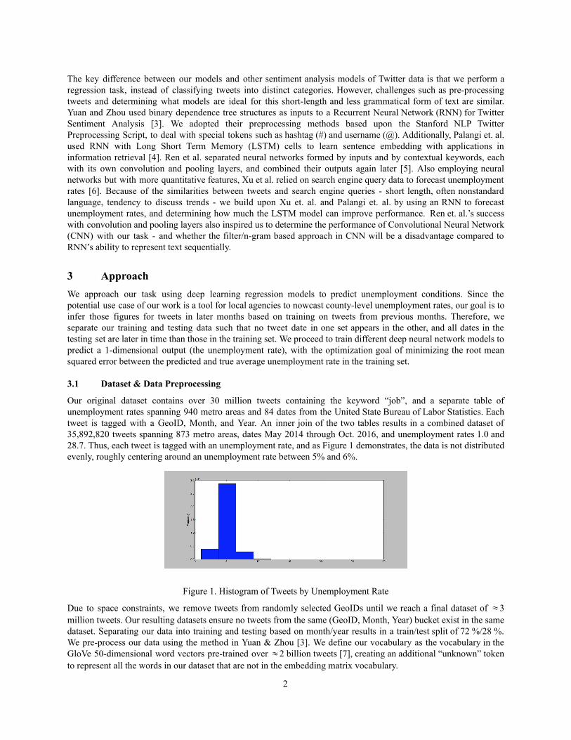
Our original dataset contains over 30 million tweets containing the keyword “job”, and a separate table of                                 unemployment rates spanning 940 metro areas and 84 dates from the United State Bureau of Labor Statistics. Each                                   tweet is tagged with a GeoID, Month, and Year. An inner join of the two tables results in a combined dataset of                                           35,892,820 tweets spanning 873 metro areas, dates May 2014 through Oct. 2016, and unemployment rates 1.0 and                                 28.7. Thus, each tweet is tagged with an unemployment rate, and as Figure 1 demonstrates, the data is not distributed                                       evenly,   roughly   centering   around   an   unemployment   rate   between   5%   and   6%.  

 

 

 

 

 

 

 

Figure   1.   Histogram   of   Tweets   by   Unemployment   Rate 

Due to space constraints, we remove tweets from randomly selected GeoIDs until we reach a final dataset of 3                                       million tweets. Our resulting datasets ensure no tweets from the same (GeoID, Month, Year) bucket exist in the same                                     dataset. Separating our data into training and testing based on month/year results in a train/test split of 72 %/28 %.                                       We pre­process our data using the method in Yuan & Zhou [3]. We define our vocabulary as the vocabulary in the                                         GloVe 50­dimensional word vectors pre­trained over 2 billion tweets [7], creating an additional “unknown” token                               to   represent   all   the   words   in   our   dataset   that   are   not   in   the   embedding   matrix   vocabulary.  

2 

 

3.2 Baseline 

We ran two baseline models to predict unemployment rate. We first create a model that assumes the unemployment                                   in a (GeoID, Month, Year) bucket is the same as the unemployment at the corresponding (GeoID, (Month­1) % 12,                                     Year) bucket. One would not expect drastic changes in the unemployment rate between months, hence this baseline                                 provides us a sense of how accurate prediction can be when we have the knowledge of the most recent                                     unemployment data. This baseline results in a root­mean squared (RMS) error of .58380, with the average difference                                 between the previous and current unemployment rates equal to .13977, and Spearman Correlation Coefficient of                             .95128,    p= 0.0.  

However, “nowcasting” is based on the idea that local agencies may not have access to unemployment statistics on                                   a monthly basis, and smaller communities may have to wait for a longer time to observe changes in the                                     unemployment rate. Thus, our goal is to measure how well models trained on Twitter data can come close to the                                       baseline of predicting unemployment rate based on actual previous figures, rather than surpassing this result.                             Therefore, our second baseline model is a linear regression model that takes an average of GLoVE vector                                 representations of each word in a tweet as inputs. With this model, our root­mean squared error is 1.41421 per tweet                                       and   2.38125   per   bucket,   and   we   hope   to   improve   upon   these   values   with   our   deep   learning   models.   3.3 Deep   Learning   Models 

To use Deep Learning Models for our task, we store each tweet as a sequence of index values into our embedding                                         matrix to save space, and pad each tweet with a special token corresponding to the last row of our embedding                                       matrix until a total of 20 tokens is obtained. Our embedding matrix across all models is initialized with the GloVe                                       50­d   word   vectors   pre­trained   over    2   billion   tweets,   extended   by   1   row   for   the   “not   found”   token.    

Provided word vectors as features, each model outputs a value as the unemployment rate prediction. We train the                                   models with true labels of UER corresponding to each tweet, experimenting with different deep neural architectures                               and hyper­parameters. We test our model on an unseen test­set with the following two approaches, based on the fact                                     that   every   tweet   belonging   to   the   same   (GeoID,   Month,   Year)   bucket   corresponds   to   the   same   UER.  

valuation #1 Mean Squared Error  (predict(tweet )  true(tweet ))E = 1|# tweets|

∑|# tweets|

t=1t   t

2  

valuation #2 Mean Squared Error  (( redict(tweet ))  true(bucket ))E =   1|# Buckets|

∑|# Buckets|

b=1

1|# tweets in bucket|

∑|# tweets in bucket|

t=1p t   b

2  

For our experiments, we report the RMS for both Evaluation metrics, along with a Spearman’s Rank Correlation                                 metric   between   the   model’s   predicted   ranking   of   buckets   by   unemployment   rate   and   the   true   ranking.  

 3.3.1 Recurrent   Neural   Network  

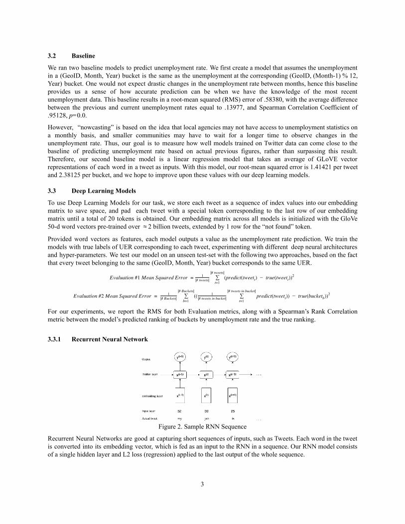
 Figure   2.   Sample   RNN   Sequence 

Recurrent Neural Networks are good at capturing short sequences of inputs, such as Tweets. Each word in the tweet                                     is converted into its embedding vector, which is fed as an input to the RNN in a sequence. Our RNN model consists                                           of   a   single   hidden   layer   and   L2   loss   (regression)   applied   to   the   last   output   of   the   whole   sequence.    

3 

 

3.3.2 Long   Short­term   Memory  

  

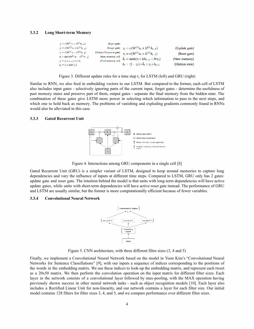
Figure   3.   Different   update   rules   for   a   time   step   t,   for   LSTM   (left)   and   GRU   (right) 

Similar to RNN, we also feed in embedding vectors to our LSTM. But compared to the former, each cell of LSTM                                         

also includes input gates ­ selectively ignoring parts of the current input, forget gates ­ determine the usefulness of                                     

past memory states and preserve part of them, output gates ­ separate the final memory from the hidden state. The                                       

combination of these gates give LSTM more power in selecting which information to pass to the next steps, and                                     

which one to hold back as memory. The problems of vanishing and exploding gradients commonly found in RNNs                                   

would   also   be   alleviated   in   this   case.  

 

3.3.3 Gated   Recurrent   Unit  

  

 

 

 

 

 

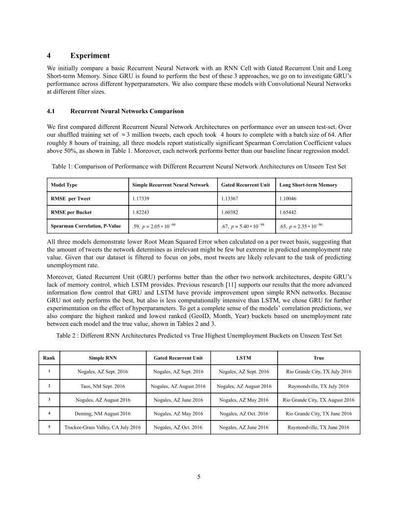
Figure   4.   Interactions   among   GRU   components   in   a   single   cell   [8] 

Gated Recurrent Unit (GRU) is a simpler variant of LSTM, designed to keep around memories to capture long                                   

dependencies and vary the influence of inputs at different time steps. Compared to LSTM, GRU only has 2 gates:                                     

update gate and reset gate. The intuition behind the model is that units with long­term dependencies will have active                                     

update gates, while units with short­term dependencies will have active reset gate instead. The performance of GRU                                 

and   LSTM   are   usually   similar,   but   the   former   is   more   computationally   efficient   because   of   fewer   variables.  

3.3.4 Convolutional   Neural   Network 

 

 

 

 

 

 

Figure   5.   CNN   architecture,   with   three   different   filter   sizes   (3,   4   and   5) 

Finally, we implement a Convolutional Neural Network based on the model in Yoon Kim’s “Convolutional Neural                               

Networks for Sentence Classifiations” [9], with our inputs a sequence of indices corresponding to the positions of                                 

the words in the embedding matrix. We use these indices to look­up the embedding matrix, and represent each tweet                                     

as a 20x50 matrix. We then perform the convolution operation on the input matrix for different filter sizes. Each                                     

layer in the network consists of a convolutional layer followed by max­pooling, with the MAX operation having                                 

previously shown success in other neural network tasks ­ such as object recognition models [10]. Each layer also                                   

includes a Rectified Linear Unit for non­linearity, and our network contains a layer for each filter size. Our initial                                     

model   contains   128   filters   for   filter   sizes   3,   4,   and   5,   and   we   compare   performance   over   different   filter   sizes.  

4 

 

4 Experiment We initially compare a basic Recurrent Neural Network with an RNN Cell with Gated Recurrent Unit and Long                                   Short­term Memory. Since GRU is found to perform the best of these 3 approaches, we go on to investigate GRU’s                                       performance across different hyperparameters. We also compare these models with Convolutional Neural Networks                         at   different   filter   sizes.  

 4.1 Recurrent   Neural   Networks   Comparison  We first compared different Recurrent Neural Network Architectures on performance over an unseen test­set. Over                             our shuffled training set of 3 million tweets, each epoch took 4 hours to complete with a batch size of 64. After                                             roughly 8 hours of training, all three models report statistically significant Spearman Correlation Coefficient values                             above   50%,   as   shown   in   Table   1.   Moreover,   each   network   performs   better   than   our   baseline   linear   regression   model.  Table   1:   Comparison   of   Performance   with   Different   Recurrent   Neural   Network   Architectures   on   Unseen   Test   Set 

 Model   Type  Simple   Recurrent   Neural   Network  Gated   Recurrent   Unit  Long   Short­term   Memory 

RMSE      per   Tweet  1.17339  1.13367  1.10046 

RMSE   per   Bucket  1.82243  1.60382  1.65442 

Spearman   Correlation,   P­Value  .59,    .05 0  p = 2 1 66  .67,    .40 0  p = 5 1 94

  .65,    .35 0  p = 2 1 86 

All three models demonstrate lower Root Mean Squared Error when calculated on a per tweet basis, suggesting that                                   the amount of tweets the network determines as irrelevant might be few but extreme in predicted unemployment rate                                   value. Given that our dataset is filtered to focus on jobs, most tweets are likely relevant to the task of predicting                                         unemployment   rate.  

Moreover, Gated Recurrent Unit (GRU) performs better than the other two network architectures, despite GRU’s                             lack of memory control, which LSTM provides. Previous research [11] supports our results that the more advanced                                 information flow control that GRU and LSTM have provide improvement upon simple RNN networks. Because                             GRU not only performs the best, but also is less computationally intensive than LSTM, we chose GRU for further                                     experimentation on the effect of hyperparameters. To get a complete sense of the models’ correlation predictions, we                                 also compare the highest ranked and lowest ranked (GeoID, Month, Year) buckets based on unemployment rate                               between   each   model   and   the   true   value,   shown   in   Tables   2   and   3.  

Table   2   :   Different   RNN   Architectures   Predicted   vs   True   Highest   Unemployment   Buckets   on   Unseen   Test   Set 

 Rank  Simple   RNN  Gated   Recurrent   Unit  LSTM  True 

1  Nogales,   AZ   Sept.   2016  Nogales,   AZ   Sept.   2016  Nogales,   AZ   Sept.   2016  Rio   Grande   City,   TX   July   2016 

2  Taos,   NM   Sept.   2016  Nogales,   AZ   August   2016  Nogales,   AZ   August   2016  Raymondville,   TX   July   2016 

3  Nogales,   AZ   August   2016  Nogales,   AZ   June   2016  Nogales,   AZ   May   2016  Rio   Grande   City,   TX   August   2016 

4  Deming,   NM   August   2016  Nogales,   AZ   May   2016  Nogales,   AZ   Oct.   2016  Rio   Grande   City,   TX   June   2016 

5  Truckee­Grass   Valley,   CA   July   2016  Nogales,   AZ   Oct.   2016  Nogales,   AZ   June   2016  Raymondville,   TX   June   2016 

 

 

5 

 

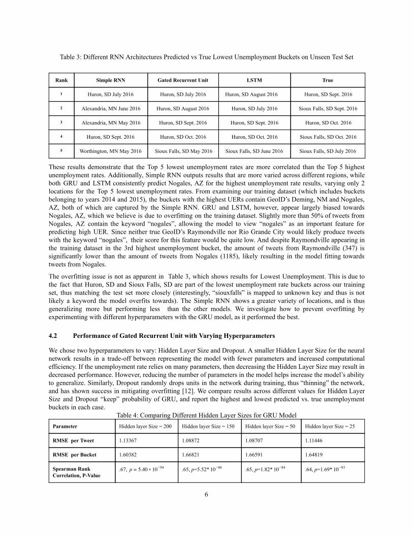
Table   3:   Different   RNN   Architectures   Predicted   vs   True   Lowest   Unemployment   Buckets   on   Unseen   Test   Set 

 

Rank  Simple   RNN  Gated   Recurrent   Unit  LSTM  True 

1  Huron,   SD   July   2016  Huron,   SD   July   2016         Huron,   SD   August   2016     Huron,   SD   Sept.   2016 

2  Alexandria,   MN   June   2016  Huron,   SD   August   2016  Huron,   SD   July   2016     Sioux   Falls,   SD   Sept.   2016 

3  Alexandria,   MN   May   2016  Huron,   SD   Sept.   2016  Huron,   SD   Sept.   2016     Huron,   SD   Oct.   2016 

4  Huron,   SD   Sept.   2016  Huron,   SD   Oct.   2016  Huron,   SD   Oct.   2016     Sioux   Falls,   SD   Oct.   2016 

5  Worthington,   MN   May   2016     Sioux   Falls,   SD   May   2016  Sioux   Falls,   SD   June   2016  Sioux   Falls,   SD   July   2016 

These results demonstrate that the Top 5 lowest unemployment rates are more correlated than the Top 5 highest                                   

unemployment rates. Additionally, Simple RNN outputs results that are more varied across different regions, while                             

both GRU and LSTM consistently predict Nogales, AZ for the highest unemployment rate results, varying only 2                                 

locations for the Top 5 lowest unemployment rates. From examining our training dataset (which includes buckets                               

belonging to years 2014 and 2015), the buckets with the highest UERs contain GeoID’s Deming, NM and Nogales,                                   

AZ, both of which are captured by the Simple RNN. GRU and LSTM, however, appear largely biased towards                                   

Nogales, AZ, which we believe is due to overfitting on the training dataset. Slightly more than 50% of tweets from                                       

Nogales, AZ contain the keyword “nogales”, allowing the model to view “nogales” as an important feature for                                 

predicting high UER. Since neither true GeoID’s Raymondville nor Rio Grande City would likely produce tweets                               

with the keyword “nogales”, their score for this feature would be quite low. And despite Raymondville appearing in                                   

the training dataset in the 3rd highest unemployment bucket, the amount of tweets from Raymondville (347) is                                 

significantly lower than the amount of tweets from Nogales (1185), likely resulting in the model fitting towards                                 

tweets   from   Nogales. 

The overfitting issue is not as apparent in Table 3, which shows results for Lowest Unemployment. This is due to                                       

the fact that Huron, SD and Sioux Falls, SD are part of the lowest unemployment rate buckets across our training                                       

set, thus matching the test set more closely (interestingly, “siouxfalls” is mapped to unknown key and thus is not                                     

likely a keyword the model overfits towards). The Simple RNN shows a greater variety of locations, and is thus                                     

generalizing more but performing less than the other models. We investigate how to prevent overfitting by                               

experimenting   with   different   hyperparameters   with   the   GRU   model,   as   it   performed   the   best.  

 4.2 Performance   of   Gated   Recurrent   Unit   with   Varying   Hyperparameters   

 We chose two hyperparameters to vary: Hidden Layer Size and Dropout. A smaller Hidden Layer Size for the neural                                     

network results in a trade­off between representing the model with fewer parameters and increased computational                             

efficiency. If the unemployment rate relies on many parameters, then decreasing the Hidden Layer Size may result in                                   

decreased performance. However, reducing the number of parameters in the model helps increase the model’s ability                               

to generalize. Similarly, Dropout randomly drops units in the network during training, thus “thinning” the network,                               

and has shown success in mitigating overfitting [12]. We compare results across different values for Hidden Layer                                 

Size and Dropout “keep” probability of GRU, and report the highest and lowest predicted vs. true unemployment                                 

buckets   in   each   case.  

Table   4:   Comparing   Different   Hidden   Layer   Sizes   for   GRU   Model 

Parameter  Hidden   layer   Size   =   200  Hidden   layer   Size   =   150  Hidden   layer   Size   =   50  Hidden   layer   Size   =   25 

RMSE      per   Tweet  1.13367  1.08872  1.08707  1.11446 

RMSE      per   Bucket  1.60382  1.66821  1.66591  1.64819 

Spearman   Rank Correlation,   P­Value 

.67,    .40 0  p = 5 1 94   .65,    p =5.52* 01 86   .65,    p =1.82* 01 84   .64,    p =1.69* 01 83  

6 

 

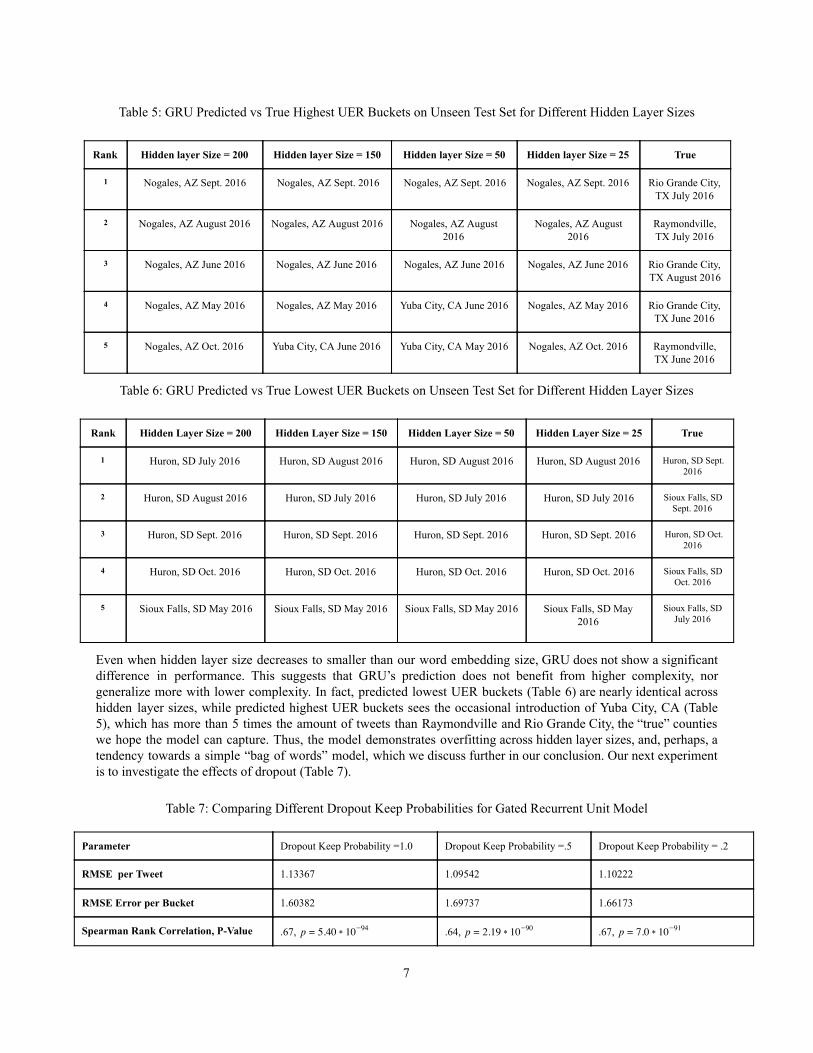
Table   5:   GRU   Predicted   vs   True   Highest   UER   Buckets   on   Unseen   Test   Set   for   Different   Hidden   Layer   Sizes  

Rank  Hidden   layer   Size   =   200  Hidden   layer   Size   =   150  Hidden   layer   Size   =   50  Hidden   layer   Size   =   25  True 

1  Nogales,   AZ   Sept.   2016     Nogales,   AZ   Sept.   2016      Nogales,   AZ   Sept.   2016  Nogales,   AZ   Sept.   2016  Rio   Grande   City, TX   July   2016 

2  Nogales,   AZ   August   2016  Nogales,   AZ   August   2016  Nogales,   AZ   August 2016 

Nogales,   AZ   August 2016 

Raymondville, TX   July   2016 

3  Nogales,   AZ   June   2016  Nogales,   AZ   June   2016  Nogales,   AZ   June   2016  Nogales,   AZ   June   2016  Rio   Grande   City, TX   August   2016 

4  Nogales,   AZ   May   2016  Nogales,   AZ   May   2016  Yuba   City,   CA   June   2016  Nogales,   AZ   May   2016  Rio   Grande   City, TX   June   2016 

5  Nogales,   AZ   Oct.   2016  Yuba   City,   CA   June   2016  Yuba   City,   CA   May   2016  Nogales,   AZ   Oct.   2016  Raymondville, TX   June   2016 

Table   6:   GRU   Predicted   vs   True   Lowest   UER   Buckets   on   Unseen   Test   Set   for   Different   Hidden   Layer   Sizes  

Rank  Hidden   Layer   Size   =   200  Hidden   Layer   Size   =   150  Hidden   Layer   Size   =   50  Hidden   Layer   Size   =   25  True 

1  Huron,   SD   July   2016   Huron,   SD   August   2016  Huron,   SD   August   2016    Huron,   SD   August   2016       Huron,   SD   Sept. 2016 

2  Huron,   SD   August   2016  Huron,   SD   July   2016   Huron,   SD   July   2016   Huron,   SD   July   2016      Sioux   Falls,   SD Sept.   2016 

3  Huron,   SD   Sept.   2016  Huron,   SD   Sept.   2016  Huron,   SD   Sept.   2016  Huron,   SD   Sept.   2016     Huron,   SD   Oct. 2016 

4  Huron,   SD   Oct.   2016  Huron,   SD   Oct.   2016  Huron,   SD   Oct.   2016  Huron,   SD   Oct.   2016     Sioux   Falls,   SD Oct.   2016 

5     Sioux   Falls,   SD   May   2016  Sioux   Falls,   SD   May   2016  Sioux   Falls,   SD   May   2016  Sioux   Falls,   SD   May 2016 

Sioux   Falls,   SD July   2016 

 

Even when hidden layer size decreases to smaller than our word embedding size, GRU does not show a significant                                     difference in performance. This suggests that GRU’s prediction does not benefit from higher complexity, nor                             generalize more with lower complexity. In fact, predicted lowest UER buckets (Table 6) are nearly identical across                                 hidden layer sizes, while predicted highest UER buckets sees the occasional introduction of Yuba City, CA (Table                                 5), which has more than 5 times the amount of tweets than Raymondville and Rio Grande City, the “true” counties                                       we hope the model can capture. Thus, the model demonstrates overfitting across hidden layer sizes, and, perhaps, a                                   tendency towards a simple “bag of words” model, which we discuss further in our conclusion. Our next experiment                                   is   to   investigate   the   effects   of   dropout   (Table   7).   

Table   7:   Comparing   Different   Dropout   Keep   Probabilities   for   Gated   Recurrent   Unit   Model  

Parameter  Dropout   Keep   Probability   =1.0  Dropout   Keep   Probability   =.5  Dropout   Keep   Probability   =   .2 

RMSE      per   Tweet  1.13367  1.09542  1.10222 

RMSE   Error   per   Bucket  1.60382  1.69737  1.66173 

Spearman   Rank   Correlation,   P­Value  .67,    .40 0  p = 5 1 94   .64,    .19 0  p = 2 1 90   .67,    .0 0  p = 7 1 91  

7 

 

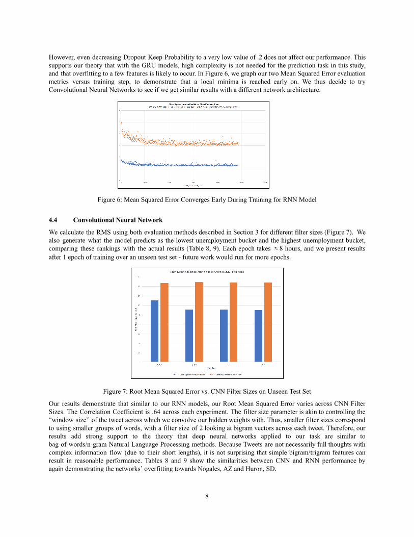
However, even decreasing Dropout Keep Probability to a very low value of .2 does not affect our performance. This                                     supports our theory that with the GRU models, high complexity is not needed for the prediction task in this study,                                       and that overfitting to a few features is likely to occur. In Figure 6, we graph our two Mean Squared Error evaluation                                           metrics versus training step, to demonstrate that a local minima is reached early on. We thus decide to try                                     Convolutional   Neural   Networks   to   see   if   we   get   similar   results   with   a   different   network   architecture.  

 

 

 

 

 

 

 

 

Figure   6:   Mean   Squared   Error   Converges   Early   During   Training   for   RNN   Model 

 4.4 Convolutional   Neural   Network 

We calculate the RMS using both evaluation methods described in Section 3 for different filter sizes (Figure 7). We                                     also generate what the model predicts as the lowest unemployment bucket and the highest unemployment bucket,                               comparing these rankings with the actual results (Table 8, 9). Each epoch takes 8 hours, and we present results                                       after   1   epoch   of   training   over   an   unseen   test   set   ­   future   work   would   run   for   more   epochs.  

 

 

 

 

 

 

 

 

 

 

Figure   7:   Root   Mean   Squared   Error   vs.   CNN   Filter   Sizes   on   Unseen   Test   Set 

Our results demonstrate that similar to our RNN models, our Root Mean Squared Error varies across CNN Filter                                   Sizes. The Correlation Coefficient is .64 across each experiment. The filter size parameter is akin to controlling the                                   “window size” of the tweet across which we convolve our hidden weights with. Thus, smaller filter sizes correspond                                   to using smaller groups of words, with a filter size of 2 looking at bigram vectors across each tweet. Therefore, our                                         results add strong support to the theory that deep neural networks applied to our task are similar to                                   bag­of­words/n­gram Natural Language Processing methods. Because Tweets are not necessarily full thoughts with                         complex information flow (due to their short lengths), it is not surprising that simple bigram/trigram features can                                 result in reasonable performance. Tables 8 and 9 show the similarities between CNN and RNN performance by                                 again   demonstrating   the   networks’   overfitting   towards   Nogales,   AZ   and   Huron,   SD.  

 

8 

 

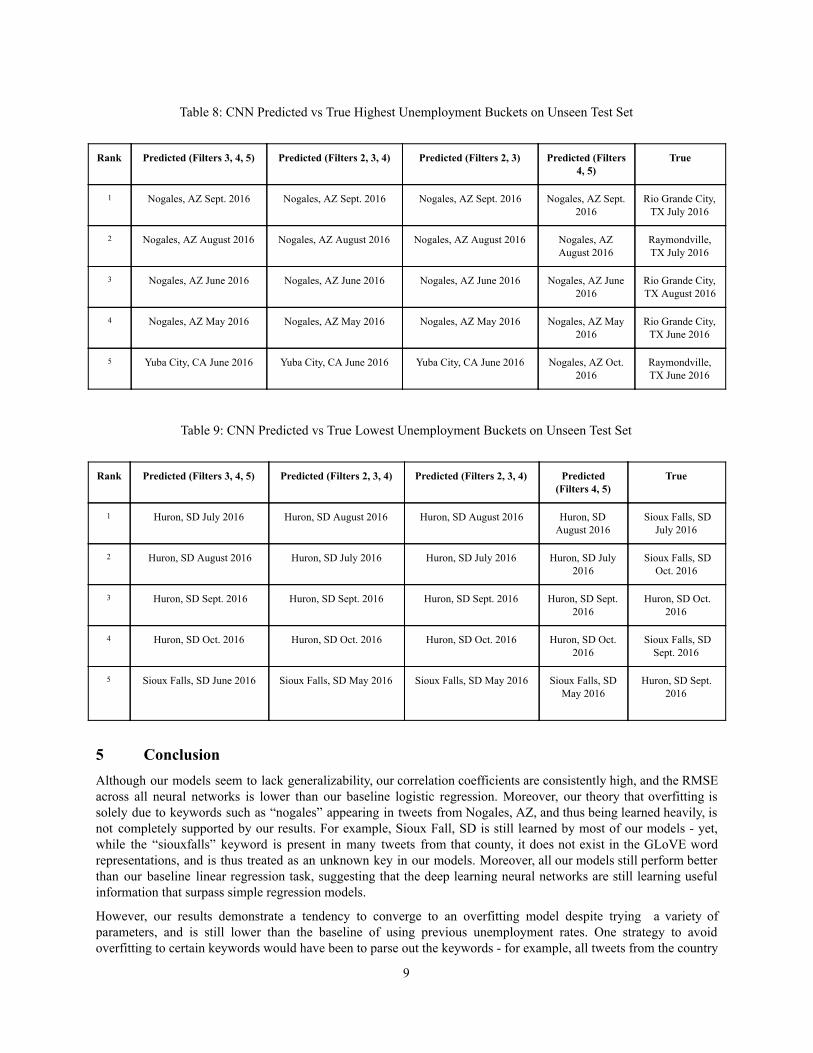
Table   8:   CNN   Predicted   vs   True   Highest   Unemployment   Buckets   on   Unseen   Test   Set 

 Rank  Predicted   (Filters   3,   4,   5)  Predicted   (Filters   2,   3,   4)  Predicted   (Filters   2,   3)  Predicted   (Filters 

4,   5) True 

1  Nogales,   AZ   Sept.   2016  Nogales,   AZ   Sept.   2016  

Nogales,   AZ   Sept.   2016  

Nogales,   AZ   Sept. 2016   

Rio   Grande   City, TX   July   2016 

2  Nogales,   AZ   August   2016  Nogales,   AZ   August   2016  Nogales,   AZ   August   2016  Nogales,   AZ August   2016 

Raymondville, TX   July   2016 

3  Nogales,   AZ   June   2016  Nogales,   AZ   June   2016  Nogales,   AZ   June   2016  Nogales,   AZ   June 2016 

Rio   Grande   City, TX   August   2016 

4  Nogales,   AZ   May   2016  Nogales,   AZ   May   2016  Nogales,   AZ   May   2016  Nogales,   AZ   May 2016 

Rio   Grande   City, TX   June   2016 

5  Yuba   City,   CA   June   2016  Yuba   City,   CA   June   2016  Yuba   City,   CA   June   2016  Nogales,   AZ   Oct. 2016 

Raymondville, TX   June   2016 

 

Table   9:   CNN   Predicted   vs   True   Lowest   Unemployment   Buckets   on   Unseen   Test   Set 

 Rank  Predicted   (Filters   3,   4,   5)  Predicted   (Filters   2,   3,   4)  Predicted   (Filters   2,   3,   4)  Predicted 

(Filters   4,   5) True 

1  Huron,   SD   July   2016  Huron,   SD   August   2016   Huron,   SD   August   2016   Huron,   SD August   2016  

   Sioux   Falls,   SD July   2016 

2     Huron,   SD   August   2016  Huron,   SD   July   2016  Huron,   SD   July   2016  Huron,   SD   July 2016 

   Sioux   Falls,   SD Oct.   2016 

3     Huron,   SD   Sept.   2016  Huron,   SD   Sept.   2016  Huron,   SD   Sept.   2016  Huron,   SD   Sept. 2016 

   Huron,   SD   Oct. 2016 

4  Huron,   SD   Oct.   2016  Huron,   SD   Oct.   2016  Huron,   SD   Oct.   2016  Huron,   SD   Oct. 2016 

   Sioux   Falls,   SD Sept.   2016 

5  Sioux   Falls,   SD   June   2016  Sioux   Falls,   SD   May   2016  Sioux   Falls,   SD   May   2016  Sioux   Falls,   SD May   2016 

Huron,   SD   Sept. 2016  

 5 Conclusion Although our models seem to lack generalizability, our correlation coefficients are consistently high, and the RMSE                               across all neural networks is lower than our baseline logistic regression. Moreover, our theory that overfitting is                                 solely due to keywords such as “nogales” appearing in tweets from Nogales, AZ, and thus being learned heavily, is                                     not completely supported by our results. For example, Sioux Fall, SD is still learned by most of our models ­ yet,                                         while the “siouxfalls” keyword is present in many tweets from that county, it does not exist in the GLoVE word                                       representations, and is thus treated as an unknown key in our models. Moreover, all our models still perform better                                     than our baseline linear regression task, suggesting that the deep learning neural networks are still learning useful                                 information   that   surpass   simple   regression   models.  

However, our results demonstrate a tendency to converge to an overfitting model despite trying a variety of                                 parameters, and is still lower than the baseline of using previous unemployment rates. One strategy to avoid                                 overfitting to certain keywords would have been to parse out the keywords ­ for example, all tweets from the country                                       

9 

 

Nogales, AZ could have been stripped of the keyword “nogales” before being processed as inputs to the networks.                                   Such preprocessing would force the network to learn representations beyond these keywords. However, new biases                             may still creep up ­ it is a difficult task to predict every keyword that is unique to a certain county. Moreover,                                           overfitting to keywords from past tweets and making them high indicators is similar to our assumption that previous                                   unemployment rates are similar to current figures in every location, and in this manner our deep learning models are                                     picking   up   signals   from   past   language   information.  

One other way to avoid overfitting is to change our train/test split strategy ­ instead of splitting across dates, we split                                         across GeoID’s. Therefore, no tweets from the same location appear in both the train and test set, and the networks                                       cannot learn location­specific keywords from the tweets. Preliminary results demonstrate RMSE per Tweet value of                             1.30510, RMSE per Bucket value of 1.53097, and a Spearman Correlation value of .69, the highest value seen so far                                       ( a full report of our results is found in the Appendix) on an unseen test set. This result is highly promising ­ the test                                                 set   prevents   the   network   from   using   any   location­specific   features,   yet   the   network   slightly   gains   in   performance.  

Overall, our models consistently report positive correlation scores above 50% and Root Mean Square Values around                               1 ­ suggesting that simply training neural networks on word features is enough for a decent performance in                                   predicting county­level unemployment rate. Future work will hopefully lead us to understand more about the nature                               of model overfitting beyond location­specific features, and expand our models to work with the full dataset of 30                                   million Tweets. Twitter is a powerful source of information about different communities around the United States ­                                 empowering small cities and towns to use the information written by and expressed by their community members is                                   a   valuable   way   to   fight   the   challenging   effects   of   unemployment. 

 

We would like to thank our mentors Dr. Patrick Baylis and Kevin Clark, and the CS224N Course Staff for their                                       support.  

 

 

 

 

 

 

 

 

 

 

 

 

 

 

 

 

 

 

 

 

10 

 

 References [1]  M. W. Linn, R. Sandifer, S. Stein. “Effects of unemployment on mental and physical health”.  American Journal                                   

of   Public   Health   75.5    (1985):   502­506.   Web.   5   March   2017. 

[2] Takeshi Sakaki, Makoto Okazaki and Yutaka Matsuo. “Earthquake shakes Twitter users: real­time event                           detection by social sensors”.  Proceedings of the 19th international conference on World wide web (2010): 851­860.                               Web.   5   March   2017. 

[3] Ye Yuan and You Zhou, “Twitter Sentiment Analysis with Recursive Neural Networks,”  CS224D Course                             

Projects    (2015).   Web.   8   Feb   2017. 

[4] Hamid Palangi, Li Deng, Yelong Shen, Jianfeng Gao, Xiaodong He, Jianshu Chen, Xinying Song, & Rabab                                 Ward. “Deep Sentence Embedding Using Long Short­Term Memory Networks: Analysis and Application to                         Information   Retrieval”.       arXiv.org    (2016).   Web.   8   Feb   2017. 

[5] Tafeng Ren, Tue Zhang, Meishan Zhang and Donghong Ji. “Context­Sensitive Twitter Sentiment Classification                           Using Neural Network”.  Proceedings of the Thirtieth AAAI Conference on Artificial Intelligence  (2016): 215­221.                           Web.   8   Feb   2017. 

[6] Wei Xu, Ziang Li and Qing Chen. “Forecasting the Unemployment Rate by Neural Networks Using Search                                 Engine   Query   Data”.    45th   Hawaii   International   Conference   on   System   Sciences    (2012).   Web.   8   Feb   2017. 

[7] Jeffrey Pennington, Richard Socher and Christopher D. Manning. “GloVe: Global Vectors for Word                           Representation”.    Empirical   Methods   in   Natural   Language   Processing   (EMNLP)    (2014).   Web.   5   Feb   2017.  

[8]   “Deep   Learning   Workshop”.   Red   Cat   Labs   (2016).   Web.   16   March   2016. 

[9] Yoon Kim. “Convolutional Neural Networks for Sentence Classification”.  Empirical Methods in Natural                         

Language   Processing   (EMNLP)    (2014).   Web.   10   March   2016. 

[10] Maximilian Riesenhuber and Tomaso Poggio. “Hierarchical models of object recognition in cortex”.  Nature                           

Neuroscience    Vol.   2   No.   11     (1999).   Web.   16   March   2016. 

[11] Junyoung Chung, Caglar Gulcehre, KyungHyun Cho and Yoshua Bengio. “Empirical Evaluation of Gated                           Recurrent   Neural   Networks   on   Sequence   Modeling”.    arXiv.org    (2014).   Web.   18   March   2017. 

[12] Nitish Srivastava, Geoffrey Hinton, Alex Krizhevsky, Ilya Sutskever and Ruslan Salakhutdinov. “Dropout: A                           Simple Way to Prevent Neural Networks from Overfitting”.  Journal of Machine Learning Research Vol. 15 (2014).                               Web.   18   March   2017. 

 

 

 

 

 

 

 

 

 

 

 

 

11 

 

 

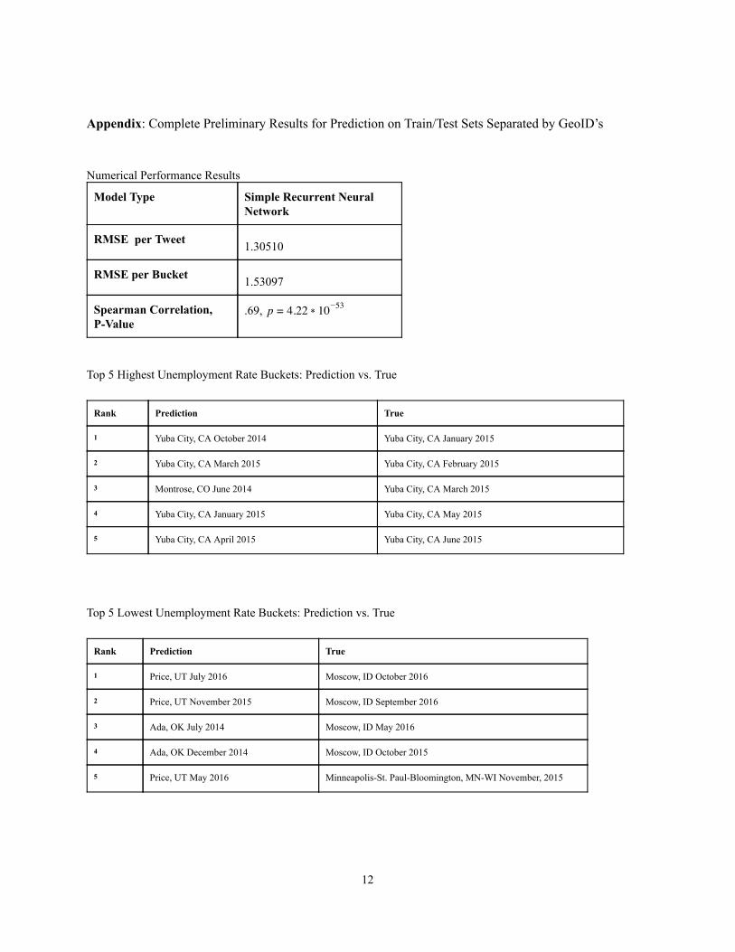
Appendix :   Complete   Preliminary   Results   for   Prediction   on   Train/Test   Sets   Separated   by   GeoID’s 

 

 Numerical   Performance   Results 

Model   Type  Simple   Recurrent   Neural Network 

RMSE      per   Tweet 1.30510 

RMSE   per   Bucket 1.53097 

Spearman   Correlation, P­Value 

.69,    .22 0  p = 4 1 53 

 

Top   5   Highest   Unemployment   Rate   Buckets:   Prediction   vs.   True  

 

Rank  Prediction  True 

1  Yuba   City,   CA   October   2014  Yuba   City,   CA   January   2015 

2  Yuba   City,   CA   March   2015  Yuba   City,   CA   February   2015 

3  Montrose,   CO   June   2014  Yuba   City,   CA   March   2015 

4  Yuba   City,   CA   January   2015  Yuba   City,   CA   May   2015 

5  Yuba   City,   CA   April   2015  Yuba   City,   CA   June   2015 

 

 

Top   5   Lowest   Unemployment   Rate   Buckets:   Prediction   vs.   True  

 

Rank  Prediction  True 

1  Price,   UT   July   2016  Moscow,   ID   October   2016 

2  Price,   UT   November   2015  Moscow,   ID   September   2016 

3  Ada,   OK   July   2014  Moscow,   ID   May   2016 

4  Ada,   OK   December   2014  Moscow,   ID   October   2015 

5  Price,   UT   May   2016  Minneapolis­St.   Paul­Bloomington,   MN­WI   November,   2015 

 

12