In Cooperation With the Ohio Lake Erie Office, Northeast Ohio Regional Sewer District, Cuyahoga County Board of Health, and U.S. Environmental Protection Agency Region 5, Water Division

Nowcasting Beach Advisories at Ohio Lake Erie Beaches

By Donna S. Francy and Robert A. Darner

Open File Report 2007–1427

U.S. Department of the Interior U.S. Geological Survey

U.S. Department of the Interior DIRK KEMPTHORNE, Secretary

U.S. Geological Survey Mark D. Myers, Director

U.S. Geological Survey, Reston, Virginia 2007

For product and ordering information: World Wide Web: http://www.usgs.gov/pubprod Telephone: 1-888-ASK-USGS

For more information on the USGS—the Federal source for science about the Earth, its natural and living resources, natural hazards, and the environment: World Wide Web: http://www.usgs.gov Telephone: 1-888-ASK-USGS

Suggested citation: Francy, D.S., and Darner, R.A., 2007, Nowcasting beach advisories at Ohio Lake Erie beaches: U.S. Geological Survey Open-File Report 2007–1427, 13 p.

Any use of trade, product, or firm names is for descriptive purposes only and does not imply endorsement by the U.S. Government.

Although this report is in the public domain, permission must be secured from the individual copyright owners to reproduce any copyrighted material contained within this report.

ii

Contents Abstract................................................................................................................................................................................1 Introduction .........................................................................................................................................................................1 Methods ...............................................................................................................................................................................2

Analytical Methods ........................................................................................................................................................2 Variables for Model Development...............................................................................................................................4 Testing and Development of Predictive Models.......................................................................................................5

Results ..................................................................................................................................................................................5 Performance of the Models in 2007.............................................................................................................................5 Exploratory Data Analysis .............................................................................................................................................6 Model Development, Diagnosis, and Selection for 2008 .........................................................................................6

Next Steps............................................................................................................................................................................7 Acknowledgments..............................................................................................................................................................7 References...........................................................................................................................................................................8

Figures 1. Map showing location of study area. ........................................................................................................................3 2. Photo of wave-height measuring buoy in the nearshore area at Edgewater, Cleveland, Ohio.....................3

Tables

1. Variables, model properties, and model responses as compared to using previous day's Escherichia coli (E. coli) concentrations in 2007. ...............................................................................................9

2. False-negative and false-positive responses for predictive models as a percentage of total exceedances and non-exceedances of the bathing-water standard, respectively, for different data segments, by date ..........................................................................................................................................................................10

3. Pearson's r correlations between log10 Escherichia coli (E. coli) concentrations and explanatory variables at three Lake Erie beaches, 2000–2007.............................................................................................11

4. Examination of candidate Huntington 2000–2007 models. ....................................................................................12 5. Examination of candidate Edgewater models for 2004–7 .....................................................................................13

iii

Conversion Factors Multiply By To obtain

inch (in.) 2.54 centimeter (cm)

inch (in.) 25.4 millimeter (mm)

foot (ft) 0.3048 meter (m)

mile (mi) 1.609 kilometer (km)

kilometer (km) 0.6214 mile (mi)

millliter (mL) 0.03381 ounce, fluid (fl. oz)

Temperature in degrees Celsius (°C) may be converted to degrees Fahrenheit (°F) as follows:

°F=(1.8×°C)+32 Bacteria concentrations are given in colony-forming units per 100 milliliters (CFU/100 mL). Pore sizes of filters are given in micrometers (µm).

iv

Nowcasting Beach Advisories at Ohio Lake Erie Beaches

By Donna S. Francy and Robert A. Darner

Abstract Data were collected during the recreational season of 2007 to test and refine predictive models at

three Ohio Lake Erie beaches. In addition to Escherichia coli (E. coli) concentrations, field personnel collected or compiled data for environmental and water-quality variables expected to affect E. coli concentrations including turbidity, wave height, water temperature, lake level, rainfall, and antecedent dry days and wet days. At Huntington (Bay Village) and Edgewater (Cleveland) during 2007, the models gave correct responses 82.7 and 82.1 percent of the time; these percentages were greater than percentages obtained by use of the previous day’s E. coli concentrations (current method). In contrast, at Villa Angela during 2007, the model gave correct responses only 61.3 percent of the days monitored; this percentage was lower than that achieved by use of the current method (74.6 percent). To refine the Huntington and Edgewater models, data from 2007 were added to existing datasets, and the larger datasets were split into two or three segments by date. Models were developed for dated segments and for combined datasets. At Huntington, the summed responses for separate best models for dated segments resulted in a greater percentage of correct responses (85.6 percent) than the one combined best model (83.1 percent). Similar results were found for Edgewater. Water-resource managers will determine how to apply these models to the Internet-based “nowcast” system for issuing water-quality advisories during 2008.

Introduction Swim advisories are issued by beach managers on the basis of standards for concentrations of

bacterial indicators—Escherichia coli (E. coli) or enterococci for freshwaters and enterococci for marine waters. At Ohio beaches, advisories are issued if the previous day’s E. coli concentration exceeds the single-sample bathing-water standard of 235 colony-forming units per 100 milliliters (CFU/100 mL) (Ohio Department of Health, 2007). Because it takes 18–24 hours to obtain results and recreational water-quality conditions may change overnight, water-resource managers may issue inappropriate advisories based on erroneous assessments of current public-health risk. As a result of this time-lag issue, some agencies have turned to predictive modeling to obtain near-real-time estimates of recreational water quality.

In an earlier study, predictive models were shown to be real-time alternatives to traditional monitoring methods at Ohio beaches (Francy and others, 2006). The best model for each beach was based on a unique combination of “variables” that explained changes in E. coli concentrations. The variables included turbidity (water clarity), rainfall, wave height, water temperature, day of the year, and lake level. The output from each model was the probability that the Ohio single-sample bathing water standard would be exceeded. A threshold probability established for each beach was based on historical data. The threshold was the probability associated with too great a risk to allow swimming—a probability that would warrant the issuance of a bathing-water advisory. This approach results in estimated probabilities similar to those in a weather forecast. At one beach, Huntington (Bay Village), predictions based on a

model have been available to the public through an Internet-based nowcasting system (www.Ohionowcast.info) since May 30, 2006.

The U.S. Geological Survey (USGS), in cooperation with the Ohio Lake Erie Office, Northeast Ohio Regional Sewer District, and Cuyahoga County Board of Health, continued the development, testing, and refinement of predictive models at Huntington and two other Lake Erie beaches—Edgewater and Villa Angela (Cleveland) (fig. 1). The Huntington model (2000–2006) used for the nowcast during 2007 contained the variables log turbidity, wave height, rainfall (radar and airport), and day of the year. The Huntington model resulted in more correct responses than use of the previous day’s E. coli during 2007. The Edgewater model (2004–6), with variables log turbidity, wave height, radar rainfall, and lake level, also resulted in more correct responses than use of the previous day’s E. coli during 2007. At Villa Angela, however, the model (2004–6) with variables log turbidity, rainfall, and water temperature did not result in more accurate predictions than use of the previous day’s E. coli during 2007. Investigators continued to work on improving the predictive abilities of the Huntington and Edgewater models for the nowcast by developing bi-phase seasonal models for 2008.

Methods Daily data were collected during the recreational season of 2007 (late May through early

September) and included analyses of water samples for E. coli concentrations and measurements of explanatory variables for model development and testing. Data were collected at Huntington 7 days per week by Cuyahoga County Board of Health (CCBH) personnel and at Edgewater and Villa Angela on Monday−Friday by Northeast Ohio Regional Sewer District (NEORSD) personnel. These agencies were also responsible for running the predictive models each morning using Fortran programs developed by the USGS. The CCBH updated the nowcast Web site daily by 9:30 a.m. with water-quality advisories and other information based on the model; model results at Edgewater and Villa Angela were compiled in a spreadsheet.

Samples were collected between 8 and 10 a.m. where the water was 2−3 ft deep in two areas of each beach used for swimming. All water-sample bottles were filled about 1 ft below the water surface by means of a grab-sampling technique (Myers and Wilde, 2003). Water samples were kept on ice and analyzed for concentrations of E. coli and turbidity within 6 hours of collection. The average value from the two water samples was used for data analysis and model development.

Analytical Methods

In the Cuyahoga County Sanitary Engineers (CCSE) Laboratory for Huntington or the NEORSD Laboratory for Edgewater and Villa Angela, samples were analyzed by use of the modified mTEC membrane-filtration method (U.S. Environmental Protection Agency, 2006). In accordance with this method, bacteria were concentrated from the water sample by filtration through a 0.45-μm-pore-size filter. Filters, representing varying volumes of sample, were then placed onto modified mTEC agar plates and incubated at 35°C for 2 hours and then at 44.5°C for an additional 22 to 24 hours. Magenta-colored colonies visible after incubation were counted as E. coli and reported as CFU/100 mL. Turbidity was determined in water samples with a turbidimeter onsite (Huntington) or in the laboratory (Edgewater and Villa Angela) and reported in nephelometric turbidity ratio units (NTRUs).

2

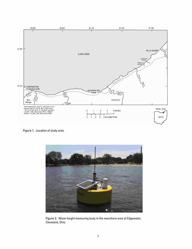
Figure 1. Location of study area.

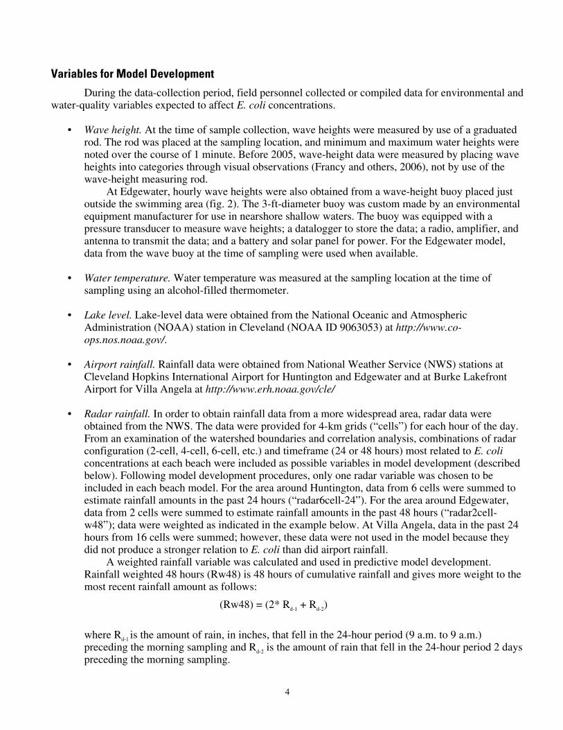
Figure 2. Wave-height measuring buoy in the nearshore area at Edgewater, Cleveland, Ohio.

3

Variables for Model Development

During the data-collection period, field personnel collected or compiled data for environmental and water-quality variables expected to affect E. coli concentrations.

• Wave height. At the time of sample collection, wave heights were measured by use of a graduated

rod. The rod was placed at the sampling location, and minimum and maximum water heights were noted over the course of 1 minute. Before 2005, wave-height data were measured by placing wave heights into categories through visual observations (Francy and others, 2006), not by use of the wave-height measuring rod. At Edgewater, hourly wave heights were also obtained from a wave-height buoy placed just outside the swimming area (fig. 2). The 3-ft-diameter buoy was custom made by an environmental equipment manufacturer for use in nearshore shallow waters. The buoy was equipped with a pressure transducer to measure wave heights; a datalogger to store the data; a radio, amplifier, and antenna to transmit the data; and a battery and solar panel for power. For the Edgewater model, data from the wave buoy at the time of sampling were used when available.

• Water temperature. Water temperature was measured at the sampling location at the time of

sampling using an alcohol-filled thermometer. • Lake level. Lake-level data were obtained from the National Oceanic and Atmospheric

Administration (NOAA) station in Cleveland (NOAA ID 9063053) at http://www.co-ops.nos.noaa.gov/.

• Airport rainfall. Rainfall data were obtained from National Weather Service (NWS) stations at

Cleveland Hopkins International Airport for Huntington and Edgewater and at Burke Lakefront Airport for Villa Angela at http://www.erh.noaa.gov/cle/

• Radar rainfall. In order to obtain rainfall data from a more widespread area, radar data were

obtained from the NWS. The data were provided for 4-km grids (“cells”) for each hour of the day. From an examination of the watershed boundaries and correlation analysis, combinations of radar configuration (2-cell, 4-cell, 6-cell, etc.) and timeframe (24 or 48 hours) most related to E. coli concentrations at each beach were included as possible variables in model development (described below). Following model development procedures, only one radar variable was chosen to be included in each beach model. For the area around Huntington, data from 6 cells were summed to estimate rainfall amounts in the past 24 hours (“radar6cell-24”). For the area around Edgewater, data from 2 cells were summed to estimate rainfall amounts in the past 48 hours (“radar2cell-w48”); data were weighted as indicated in the example below. At Villa Angela, data in the past 24 hours from 16 cells were summed; however, these data were not used in the model because they did not produce a stronger relation to E. coli than did airport rainfall. A weighted rainfall variable was calculated and used in predictive model development. Rainfall weighted 48 hours (Rw48) is 48 hours of cumulative rainfall and gives more weight to the most recent rainfall amount as follows:

(Rw48) = (2* Rd-1 + Rd-2)

where Rd-1 is the amount of rain, in inches, that fell in the 24-hour period (9 a.m. to 9 a.m.) preceding the morning sampling and Rd-2 is the amount of rain that fell in the 24-hour period 2 days preceding the morning sampling.

4

• Antecedent dry days and wet days. The variable “antecedent dry days” was calculated by counting the number of consecutive days without measureable rainfall up to and including 9 a.m. on the date of the sampling. “Antecedent wet days” was calculated by counting the number of consecutive days with measureable rainfall up to and including 9 a.m. on the date of the sampling. Quality-assurance and quality-control (QA/QC) procedures were implemented to ensure the

collection and documentation of high-quality data. The USGS did several onsite QA/QC checks of procedures performed by field and laboratory personnel, and any needed corrective actions were taken. Duplicates, field blanks, and positive-control reference cultures for E. coli, described elsewhere (Francy and others, 2007), were analyzed by CCSE and NEORSD. For turbidity, duplicate aliquots were measured from the same bottle, and measurements that did not agree within 10 percent were repeated. Turbidity reference standards were sent to both laboratories. Results from QC samples were carefully monitored by the USGS, and retests were done or corrective measures taken when needed.

Testing and Development of Predictive Models

The models previously developed at Huntington (2000–2006) and Edgewater and Villa Angela (2004–6) were tested during 2007 (table 1). Personnel from local agencies entered daily data into a Fortran program, written by the USGS, that computed the probability of exceeding 235 CFU/100 mL based on each beach-specific model. At the end of the 2007 season, model responses were tallied. After testing, the 2007 data were added to the existing dataset, and refined models were developed for future use, when applicable. Steps to developing new models included (1) examining performance of the models during 2007, (2) performing exploratory data analysis, and (3) model development, diagnostics, and selection. Multiple linear regression (MLR) techniques were used for model development. In MLR, a unique set of variables is used to develop a model that best explains the variation in E. coli concentrations, leaving as little variation as possible to unexplained “noise.” Detailed information on the steps for developing predictive models can be found in Francy and Darner (2006).

Results

Performance of the Models in 2007

The Huntington 2000–2006 model and Edgewater and Villa Angela 2004–6 models were evaluated for their abilities to yield correct predictions and sensitivities and specificities of responses during 2007 and were compared to use of the previous day’s E. coli concentrations (table 1; all tables are at back of report). The sensitivity is the percentage of events where the model correctly predicts exceedance of the bathing-water standard among days where the standard is exceeded. The specificity is the percentage of events where the model correctly predicted nonexceedance of the standard. At Huntington and Edgewater, the models resulted in greater percentages of correct responses than use of the previous day’s E. coli concentrations (current method); the percent difference for Huntington, however, was small and not as great as that found during 2006 (see http://www.ohionowcast.info/ ohionowcastfindoutmore.htm). Also at Huntington, the model resulted in better sensitivity but similar specificity as the current method. The improved sensitivity for the model over the current method resulted in four more correct predictions when the standard was exceeded. This is important in terms of protection of public health. At Edgewater, the model resulted in both higher sensitivity and specificity than the current method. In contrast, at Villa Angela, the model resulted in correct responses only 61.3 percent of the days monitored; this percentage was lower than that achieved by use of the current method (74.6 percent). Although specificity of the model was high at Villa Angela, the sensitivity was only 32.6 percent and considerably lower than that for the current method.

5

Because of the uncertainty in the transmission of radar data, an alternative model with the same variables but without radar6cell-24 was developed for Huntington for the daily nowcast. The alternative model without radar data yielded the same percentage of correct responses, same sensitivity, and very similar specificity as the original model with radar data (data not shown).

At Huntington during 2007, 7 out of 7 false negatives occurred before July 29, and 9 out of 11 false positives occurred after July 22. A false negative occurs when the E. coli concentration exceeds the standard but the model predicts the concentration to be below the standard. A false positive occurs when the E. coli concentration meets the standard but the model predicts exceedance of the standard. The data for 2000–2007 were split into segments based on the occurrence of false negatives and positives that would have occurred in responses from the Huntington 2000–2006 model (table 2). For the data split into two or three segments, the percentages of false negatives decreased over time and the percentages of false positives increased over time. The two-segment split was used in model refinement because it was simpler than the three-segment split and it divided the season into reasonably sized segments: (1) May 21 through July 23 (“season 1”) and (2) July 24 through September 3 (“season 2”).

At Edgewater, the data for 2004–7 were similarly split into segments based on occurrence of false negatives and positives that would have occurred in responses from the Edgewater 2004–6 model. As was found for Huntington, the percentages of false negatives decreased over time, whereas the percentages of false positives increased over time (table 2). The three-segment split clearly showed this trend, and this division was later used in model refinement.

Exploratory Data Analysis

The correlations between E. coli concentrations and explanatory variables are shown for data collected in previous years and in 2007 (table 3). Correlations for wave heights measured by use of the wave rod in previous years were not included because they were measured as categorical variables before 2005. Similarly, the wave-height buoy at Edgewater became operational in late summer 2005.

At Huntington, for the variables used in the 2000–2006 model—day of the year, Rw48, radar6cell-24, and log turbidity—correlations in 2007 were the same or stronger than in previous years. Interestingly, the correlation between E. coli concentrations and wave heights measured by the buoy at Edgewater (r=0.67) was stronger than wave heights measured by use of the measuring rod at Huntington (r=0.60). Edgewater is approximately 10 mi east of Huntington along the Lake Erie shoreline.

At Edgewater, for two of the variables used in the 2004–6 model—radar2cell-48 and lake level—correlations in 2007 were stronger than in previous years. For log turbidity, however, the correlation was weaker in 2007 (r=0.33) than in previous years (r=0.47). The wave-height buoy and wave-rod measurements were equally correlated with E. coli concentrations. At Villa Angela, for the variables used in the 2004–6 model, the correlation for water temperature was slightly stronger in 2007 than for previous years. For log turbidity and Rd-1, however, the correlations were weaker during 2007 than in previous years.

Model Development, Diagnosis, and Selection for 2008

Huntington. At Huntington, explanatory variables consistently related to E. coli during 2007 and previous years were used for model development for the 2000–2007 dataset—day of the year, Rd-1, Rw48, radar6cell-24, log turbidity, and wave height. Two new variables, antecedent dry days and antecedent wet days, also were included. For data collected in 2000–2007, dry days and wet days were significantly related to E. coli (r=-0.32 and r=0.30, respectively). Data from 2000–2007 were split into two segments by date, as previously described. Models were developed for season 1, season 2, and combined datasets. Two types of models were developed: (1) simple models that used the same variables as those in the 2000–2006 model, omitting radar rainfall (log turbidity, wave height and w48) and (2) the best model for each dataset as identified by MLR techniques (Francy and Darner, 2006). Threshold probabilities were established for each simple and best model by identifying the probabilities that were reasonable balances 6

between achieving a high number of correct responses and low number of false negative responses (Francy and Darner, 2006).

In addition to standard model diagnostic procedures, such as R2 values and partial residual plots (Francy and Darner, 2006), candidate models were evaluated by examining the numbers and percentages of correct responses, false positives, and false negatives for 2000–2007 data (table 4). The summed responses for separate simple models for seasons 1 and 2 resulted in a greater percentage of correct responses (83.0 percent) than one combined simple model (81.0 percent); sensitivities were higher and specificities only slightly higher for the former; this translated into 10 more correct responses for the summed simple model over the combined simple model. Similarly, the summed responses for separate best models for seasons 1 and 2 resulted in a greater percentage of correct responses (85.6 percent) than the one combined best model (83.1 percent), translating to 19 more correct responses for the summed best model over the combined best model. The summed responses for the season 1 and 2 best models provided a higher specificity but slightly lower sensitivity than the combined best model. Of the two summed models, the best model had a greater percentage of correct responses, higher specificity, and a slightly lower sensitivity (but the same number of false negatives) as the simple summed model.

One more model was developed for Huntington. This model was the season 1 best model without radar rainfall for possible use in the event radar rainfall data are not available. A threshold probability of 20 was set to achieve similar percentages of responses as those found for the season 1 best model with radar rainfall.

Edgewater. At Edgewater, explanatory variables consistently related to E. coli during 2007 and

previous years were used for model development for the 2004–7 dataset—day of the year, Rd-1, Rw48, radar2cell-w48, log turbidity, lake level, and wave-height rod. Antecedent dry days and antecedent wet days were not included because the correlations to log E. coli (r=-0.21 and r=0.25, respectively) were lower than for the other available variables. Data from 2004–7 were split into three segments by date, as previously described. Best models and threshold probabilities were developed for season 1, season 2, season 3, and for the combined dataset (table 5).

Model diagnostics were performed in the same manner as described above for Huntington. For Edgewater, as was found for Huntington, the summed responses for separate simple models for seasons 1, 2, and 3 provided a greater percentage of correct responses (86.9 percent) than one combined simple model (84.9 percent); specificities and sensitivities were also higher for the former.

Next Steps The beach manager at Huntington will determine which 2000–2007 model to use to issue

advisories for the nowcast system during 2008. Similarly, from results in 2007, water-resource managers will decide whether predictions based on the Edgewater 2004–7 model can be used to issue advisories through the nowcast system in 2008. Because modeling is a dynamic process, models for Huntington and Edgewater should be validated and refined to improve predictions during 2008. At Villa Angela, other options will be examined, such as the use of a rapid analytical method for E. coli for issuing beach advisories.

Acknowledgments The authors would like to thank Jill Lis and Lena Kavaliauskas of the Cuyahoga County Board of

Health for sampling and running the nowcast. Thanks are also extended to collaborators Mark Citriglia, Eva Hatvani, and Lester Stumpe at the Northeast Ohio Sewer District. This project was funded in part through the Lake Erie Protection Fund, administered by the Ohio Lake Erie Commission.

7

References Francy, D.S., and Darner, R.A., 2006, Procedures for developing models to predict exceedance of

recreational water-quality standards at coastal beaches: U.S. Geological Survey Techniques and Methods 6–B5, 34 p., available at http://pubs.usgs.gov/tm/2006/tm6b5/

Francy, D.S., Darner, R.A., and Bertke, E.E., 2006, Models for predicting recreational water quality at Lake Erie beaches: U.S. Geological Survey Scientific Investigations Report 2006–5192, 13 p., available at http://pubs.usgs.gov/sir/2006/5192/

Francy, D.S., Bushon, R.N., Bertke, E.E., Brady, A.M.G., Kephart, C.M., Likirdopolus, C.A., and Stoeckel, D.M., 2007, Quality-assurance/quality-control manual for the Ohio Water Microbiology Laboratory, accessed December 2007 at http://oh.water.usgs.gov/micro_qaqc.htm

Myers, D.N., and Wilde, F.D., eds., 2003, Biological indicators (3d ed.): U.S. Geological Survey Techniques of Water-Resources Investigations, book 9, chap. A7, accessed March 2006 at http://pubs.water.usgs.gov/twri9A7/

Ohio Department of Health, 2007, Bathing beach monitoring program, accessed October 2007 at http://www.odh.state.oh.us/odhPrograms/eh/bbeach/beachmon.aspx

U.S. Environmental Protection Agency, 2006, Method 1603—Escherichia coli in water by membrane filtration using modified membrane-thermotolerant Escherichia coli agar: Washington, D.C., EPA 821–R–06–011, 42 p.

8

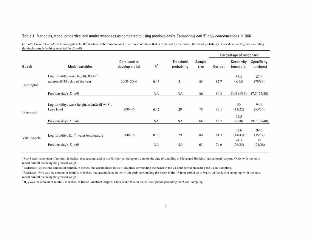
Table 1. Variables, model properties, and model responses as compared to using previous day's Escherichia coli (E. coli) concentrations in 2007.

[E. coli , Escherichia coli; NA, not applicable; R2, fraction of the variation of E. coli concentrations that is explained by the model; threshold probability is based on meeting and exceeding the single-sample bathing standard for E. coli]

Percentage of responses

Beach Model variablesData used to

develop model R2 Threshold probability

Sample size Correct

Sensitivity (numbers)

Specificity (numbers)

Huntington

Log turbidity, wave height, Rw48a,

radar6cell-24b, day of the year 2000−2006 0.43 31 104 82.753.3

(8/15)87.6

(78/89)

Previous day's E. coli NA NA 101 80.2 30.8 (4/13) 87.5 (77/88)

Edgewater

Log turbidity, wave height, radar2cell-w48c, Lake level 2004−6 0.42 29 78 82.1

50(11/22)

94.6(53/56)

Previous day's E. coli NA NA 66 66.733.3

(6/18) 79.2 (38/48)

Villa AngelaLog turbidity, Rd-1

d, water temperature 2004−6 0.32 29 80 61.332.6

(14/43)94.6

(35/37)

Previous day's E. coli NA NA 63 74.674.3

(26/35)75

(21/28)

a Rw48 was the amount of rainfall, in inches, that accumulated in the 48-hour period up to 9 a.m. on the date of sampling at Cleveland Hopkins International Airport, Ohio, with the most recent rainfall receiving the greatest weight.b Radar6cell-24 was the amount of rainfall, in inches, that accumulated in six 4-km grids surrounding the beach in the 24-hour period preceding the 9 a.m. sampling.c Radar2cell-w48 was the amount of rainfall, in inches, that accumulated in two 4-km grids surrounding the beach in the 48-hour period up to 9 a.m. on the date of sampling, with the most recent rainfall receiving the greatest weight.d Rd-1 was the amount of rainfall, in inches, at Burke Lakefront Airport, Cleveland, Ohio, in the 24-hour period preceding the 9 a.m. sampling.

9

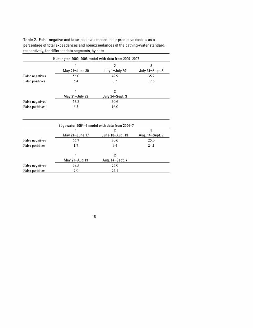
Table 2. False-negative and false-positive responses for predictive models as a percentage of total exceedances and nonexceedances of the bathing-water standard, respectively, for different data segments, by date.

Huntington 2000−2006 model with data from 2000−2007

1May 21−June 30

2July 1−July 30

3July 31−Sept. 3

False negatives 56.0 42.9 35.7False positives 5.4 8.3 17.6

1May 21−July 23

2July 24−Sept. 3

False negatives 53.8 30.6False positives 6.3 16.0

Edgewater 2004−6 model with data from 2004−71

May 21−June 172

June 18−Aug. 133

Aug. 14−Sept. 7False negatives 66.7 30.0 25.0False positives 1.7 9.4 24.1

1May 21−Aug 13

2Aug. 14−Sept. 7

False negatives 38.5 25.0False positives 7.0 24.1

10

Table 3. Pearson's r correlations between log10 Escherichia coli (E. coli) concentrations and explanatory variables at three Lake Erie beaches, 2000−2007.[Relations that were significant at p < 0.05 are in bold; ND is not determined]

Huntington Edgewater Villa Angela

Variable 2000−2006 2007 2004−6 2007 2004−6 2007Birds, number at time of sampling -0.014 ND 0.16 0.002 0.16 0.13Day of the year 0.15 0.23 0.26 0.37 -0.14 0.008

Rd-1a 0.36 0.36 0.22 0.33 0.37 0.25

Rd-2 a 0.20 0.28 ND 0.34 0.11 0.015

Rw48 b 0.39 0.42 0.28 0.40 ND NDRadar6cell-24 0.35 0.35 ND ND ND NDRadar2cell-w48 ND ND 0.33 0.41 ND NDRadar16cell-24 ND ND ND ND 0.36 NDAntecedent dry days ND ND NDAntecedent wet days ND ND NDTurbidity 0.48 0.51 0.40 0.37 0.38 0.27Log turbidity 0.53 0.53 0.47 0.33 0.35 0.30Water temperature 0.026 0.17 0.052 0.22 0.27 0.28Lake level -0.087 ND -0.25 -0.30 -0.031 ND

Wave-height buoy at Edgewater ND 0.67 ND 0.60 ND NDWave-height rod ND 0.60 ND 0.60 ND 0.40a Rd-1 was the amount, in inches, at Cleveland Hopkins International Airport or Burke Lakefront Airport, Cleveland, Ohio in the 24-hour

period preceding sampling; R d-2 was the amount 2 days before sampling. b Rw48 was the amounts, in inches, at Cleveland Hopkins International Airport or Burke Lakefront Airport, Cleveland, Ohio, in the 48-hour period before sampling, with the most recent rainfall receiving the most weight.

11

Table 4. Examination of candidate Huntington 2000-2007 models.

[R2, fraction of the variation of E. coli concentrations that is explained by the model; threshold probability is based on meeting and exceeding the single-sample bathing standard for E. coli ; season 1 is May 21-July 23 and season 2 is July 24-Sept 3; calculated sums are shaded below]

Number Percentage

Model Variables R2Threshold probability Correct False + False - Correct Sensitivity Specificity

Simple models

Season 1 Log turbidity, wave height, Rw48 0.38 21 242 35 19 81.8 63.5 85.7

Season 2 Log turbidity, wave height, Rw48 0.47 28 168 19 11 84.8 73.2 87.9

Sum of seasons 1 and 2 410 54 30 83.0 67.7 86.5

Combined Log turbidity, wave height, Rw48 0.40 31 400 58 36 81.0 61.3 85.5

Best models

Season 1 bestRw48a, radar6cell-24b, log turbidity, dry days, day of the year 0.44 25 251 27 17 85.1 66.7 88.9

Season 2 bestRw48, log turbidity, wave height, day of the year 0.48 27 170 14 13 86.3 67.5 91.1

Sum of seasons 1 and 2 421 41 30 85.6 67.0 89.8

Combined Rw48, radar6cell-24, log turbidity, wave height, dry days, wet days, 0.44 27 402 53 29 83.1 67.8 86.5

Model without radar data

Season 1 bestRw48, wave height, dry days, day of the year 0.44 20 253 25 18 85.5 65.4 89.8

a Rw48 was the amount, in inches, at Cleveland Hopkins International Airport, Ohio, in the 48-hour period before sampling, with the most recent rainfall receiving the most weight.bRadar6cell-24 was the amount of rainfall in the previous 24-hour period that fell in six 4-km grids as determined from radar data.

12

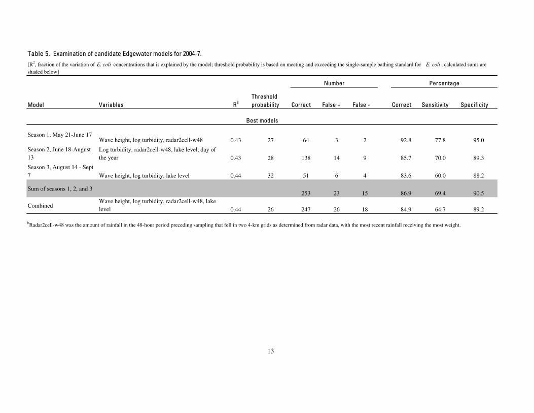
Table 5. Examination of candidate Edgewater models for 2004-7.[R2, fraction of the variation of E. coli concentrations that is explained by the model; threshold probability is based on meeting and exceeding the single-sample bathing standard for E. coli ; calculated sums are shaded below]

Number Percentage

Model Variables R2Threshold probability Correct False + False - Correct Sensitivity Specificity

Best models

Season 1, May 21-June 17Wave height, log turbidity, radar2cell-w48 0.43 27 64 3 2 92.8 77.8 95.0

Season 2, June 18-August 13

Log turbidity, radar2cell-w48, lake level, day of the year 0.43 28 138 14 9 85.7 70.0 89.3

Season 3, August 14 - Sept 7 Wave height, log turbidity, lake level 0.44 32 51 6 4 83.6 60.0 88.2

Sum of seasons 1, 2, and 3 253 23 15 86.9 69.4 90.5

Combined Wave height, log turbidity, radar2cell-w48, lake level 0.44 26 247 26 18 84.9 64.7 89.2

bRadar2cell-w48 was the amount of rainfall in the 48-hour period preceding sampling that fell in two 4-km grids as determined from radar data, with the most recent rainfall receiving the most weight.

13