Vol.:(0123456789)1 3

Acta Geophysica (2020) 68:123–132 https://doi.org/10.1007/s11600-019-00389-w

RESEARCH ARTICLE - APPLIED GEOPHYSICS

Novel wide‑angle AVO attributes using rational function

Yaru Xue1,2 · Jialin Xiang1,2 · Xin Xu1,2

Received: 3 July 2019 / Accepted: 28 November 2019 / Published online: 9 December 2019 © Institute of Geophysics, Polish Academy of Sciences & Polish Academy of Sciences 2019

AbstractConventional AVO inversion employs Zoeppritz equations and various approximations to them to obtain the reflection coef-ficients of plane-waves, which are confined to a certain (small) angle range (mostly below 40◦ ). However, near the critical angles (wide-angle), reflections at the post-critical angles provide much more potential for velocity and density inversion because of the large amplitudes and phases-shifted waveforms, while the Zoeppritz equations are not applicable anymore. Hence, there is a strong demand for the research into wide-angle AVO. With reflection coefficients at wide-angle correspond-ing to the features of rational function, we try to approximate the seismic data with vector fitting which is used to obtain the rational zero-pole and residual properties of wide-angle AVO. We apply this technique to classify AVO type and recognize the lithology. Our experiment shows that extending our research into wide-angle AVO is very promising in gathering richer data for a more accurate seismic analysis.

Keywords Seismic exploration · Lithological distinction · Wide-angle AVO · Rational function fitting

Introduction

In seismic exploration, AVO (Amplitude Variation with Off-set) is a technology which studies the lithology and detects hydrocarbon using amplitude information. The AVO inver-sion is based on the AVO characteristics to estimate the elas-tic parameters of rock and deduce the lithology of medium according to seismic data. Before inversion, the critical and post-critical reflections are traditionally muted, because NMO correction will lead to the stretching of remote off-set and to avoid the complexity of interferences of reflected and head waves (Krail and Brysk 1983; Winterstein 1985). However, with further research, it is found that the anoma-lous amplitude and phase anomalies near the critical angles

are favorable for inversion. AVO studies have shown that large-offset information is needed to extract density informa-tion. (Debski and Tarantola 1995; Downton and Ursenbach, 2006).

However, in AVO analysis, the traditional method to approximate the AVO response is by using linear formulas including the triangular function of reflection angle (Bort-feld 1961; Aki and Richards 1980; Shuey 1985). But it is only applicable at the small incidence angles, because there is a strong impedance difference near the critical angles, the Zoeppritz approximation is not applicable (O’Brien 1963; Macdonald et al. 1987). Therefore, how to characterize wide-angle AVO is an important and meaningful issue.

The introduction of long recording cables and new acqui-sition methods, such as submarine nodes, makes it possible to record large-offset reflections. The critical angle is easy to reach in structures with large velocity ratios, such as salts, volcanic rocks and carbonates. Therefore, the seismic reflec-tions at the angle above the critical angle are becoming more and more common (Zhu and Mcmechan 2015).

In general, when seismic exploration is carried out, the actual acquired seismic data are excited by the point source, which produces spherical wave (Červený and Hron 1961; Haase 2004; Ayzenberg et al. 2009; Ursenbach et al. 1949 ). And so far, a lot of studies have been devoted to the reflec-tion of spherical waves on a planar interface in two-layer

* Yaru Xue xueyaru@cup.edu.cn

* Jialin Xiang xiangjialin12@163.com

* Xin Xu XuXinIsJiangYeYe@outlook.com

1 College of Information Science and Engineering, China University of Petroleum (Beijing), Beijing 102249, China

2 State Key Laboratory of Petroleum Resources and Prospecting, China University of Petroleum (Beijing), Beijing 102249, China

124 Acta Geophysica (2020) 68:123–132

1 3

homogeneous half-space. We can find that the spherical-wave reflection coefficients are related to rational function.

Studies have found that when the incident angle is larger than the critical angle, the offset will be larger and the sig-nal-to-noise ratio of the seismic data will be higher. In the case of ignoring the loss of seismic wave energy, the energy of the wide-angle seismic reflection wave is much greater than that of the non-wide-angle reflection wave, which is a very favorable condition for the processing of seismic data. Development of wide-angle seismic exploration is very necessary.

In this paper, we use rational function to fit seismic data and characterize AVO attributes by zero-pole and residual properties. The main body of this paper is divided into two parts., fitting and applying. In the fitting part, we use rational function to fit seismic coefficient curves whose form will be elaborated in the theory, and to obtain zero-pole and residual properties and discuss the feasibility of these attributes; in the applying part, we apply this method to classify AVO, recognize hydrocarbon signatures, and compare with the traditional polynomial fitting technique. This new method is used to describe the characteristics of seismic waves more accurately, and to explore more useful information from seismic record.

Theory

AVO describes the amplitudes variation with offset, while PVO means the phases variation with offset; these two attributes can be formulated as an complex function with variable �(the incident angle):

where |H(�)| represents AVO and �(�) represents PVO; this formula is very similar to the frequency response of a cir-cuit system. Formula (1) can be expanded as summation of rational function:

where s = j2�r , Ak denotes the pole, Ck denotes the cor-responding residual for each pole, and r is defined as offset, D is the delay factor that controls the amount of delay to fit the data.

By summarizing the previous research, the spherical-wave reflection coefficient can be expressed as follows for a homogeneous half-space medium model (Li et al. 2016):

(1)H(�) = |H(�)|ei�(�)

(2)H(s) =

n∑k=1

Ck

s − Ak

+ D

where B is the plane PP-wave reflection:

v1, v2, �1, �2 denotes the P-wave velocity and density of the upper and lower medium, respectively, J0 is the zero-order Bessel function, r is the source–receiver offset ( r = (h + z) ∗ tan� ), h and z are the vertical distance from the source and the receiver to the interface, respectively, i is the imaginary unit and x = cos� , � is the angular frequency.

The formula (3) shows the spherical-wave reflection coef-ficient follows the rational function form, so we propose to use rational function (2) to fit seismic reflection coefficients and use the least-square method to solve the problem; finally, the zero-pole and residual attributes are achieved.

In the formula (2), the unknowns Ak appear in the denomi-nator, it is a nonlinear problem, so the Vector Fitting algorithm (Gustavsen and Semlyen 1999) is used to solve the problem, the nonlinear problem can become a linear problem, and then the least-square method is used to solve it.

Specify a set of initial poles Ak in (2), then multiply H(s) with a formula �(s) , where �(s) is a rational approximation to be determined; this gives the augmented problem:

Note that in (5) the rational approximation for �(s) and the approximation for �(s) H(s) have the same poles.

Multiplying the second row in (5) with H(s) draw the fol-lowing relation:

Or

Equation (6) is linear in its unknowns Ck , Ck . So writing for several incident angle points, the overdetermined linear problem is given:

(3)Rsphpp

=

∫ 0

1B(x)J0(�r

√1 − x2∕v1)e

i�x(h+z)∕v1dx

+i ∫ ∞

0B(x)J0(�r

√1 + x2∕v1)e

−�x(h+z)∕v1dx

∫ 0

1J0(�r

√1 − x2∕v1)e

i�x(h+z)∕v1dx

+i ∫ ∞

0J0(�r

√1 + x2∕v1)e

−�x(h+z)∕v1dx

(4)B(x) =�2v2x − �1v1

√1 − v2

2∕v2

1(1 − x2)

�2v2x + �1v1

√1 − v2

2∕v2

1(1 − x2)

(5)��(s)H(s)

�(s)

�=

⎛⎜⎜⎝

∑n

k=1

Ck

s−Ak

+ D

∑n

k=1

Ck

s−Ak

+ 1

⎞⎟⎟⎠

(6)n∑

k=1

Ck

s − Ak

+ D =

[n∑

k=1

Ck

s − Ak

+ 1

]H(s)

(7)(�H)fit(s) = �fit(s)H(s)

(8)Ax = b

125Acta Geophysica (2020) 68:123–132

1 3

where the unknowns are in the solution vector x . Equation (8) is solved as a least-square problem as follows: for a given incident angle �k we can get sk and:

where

Thus, a rational function approximation for H(s) is easy to get from (6) now.

If each sum of partial fractions of (6) is written as a frac-tion, it becomes obvious that it can be expressed as the form of zeros and poles:

where zk, (k = 1, 2, 3… n) are the zeros of (�H)fit(s) , Ak are the poles of �fit(s) and (�H)fit(s) , zk are the zeros of �fit(s) . Finally we can get:

Equation (14) shows the poles of H(s) become equal to the zeros of �fit(s) . Thus, by calculating the zeros of �fit(s) we can get a good set of poles for fitting the original function H(s). And the residuals for H(s) can be directly calculated from Eq. (14).

Vector Fitting is equally well suited for fitting vectors as it is for scalars. By replacing the scalar by a vector, it will result in all elements of the fitted vector sharing the same poles.

Results

Fitting

In this example, the spherical-wave reflection coefficient model of Castagna et al. (1998) and Li et al. (2016) is used, shown in Table 1, where v1, v2, �1, �2 as mentioned earlier.

(9)Akx = bk

(10)Ak =[

1

sk−A1

⋯1

sk−AN

1−H(sk)

sk−A1

⋯−H(sk)

sk−AN

]

(11)x =[c1 ⋯ cN D c1 ⋯ cN

]

(12)bk = H(sk)

(13)(�H)fit(s) = h

∏n+1

k=1(s − zk)∏n

k=1(s − Ak)

, �fit(s) =

∏n

k=1(s − zk)∏n

k=1(s − Ak)

(14)H(s) =(�H)fit(s)

�fit(s)= h

∏n+1

k=1(s − zk)∏n

k=1(s − zk)

Firstly, the rational fitting property is demonstrated by fitting the AVO coefficient curves in frequency domain. Because the spherical-wave reflection coefficient is fre-quency dependent, so in the frequency domain, the rational function fitting is done to the original wide-angle seismic data corresponding to each frequency.

The initial poles are predetermined; first, the optimum fit-ting conditions, including poles and order, of each frequency are determined by observing the relative error tolerance in the iteration. When the relative error tolerance is less than − 40 dB, the iterations are stopped and optimal fitting ampli-tude and phase are achieved. The point source has a Ricker wavelet with dominant frequency of 10 Hz, and hence we choose the curve of 10 Hz to analysis.

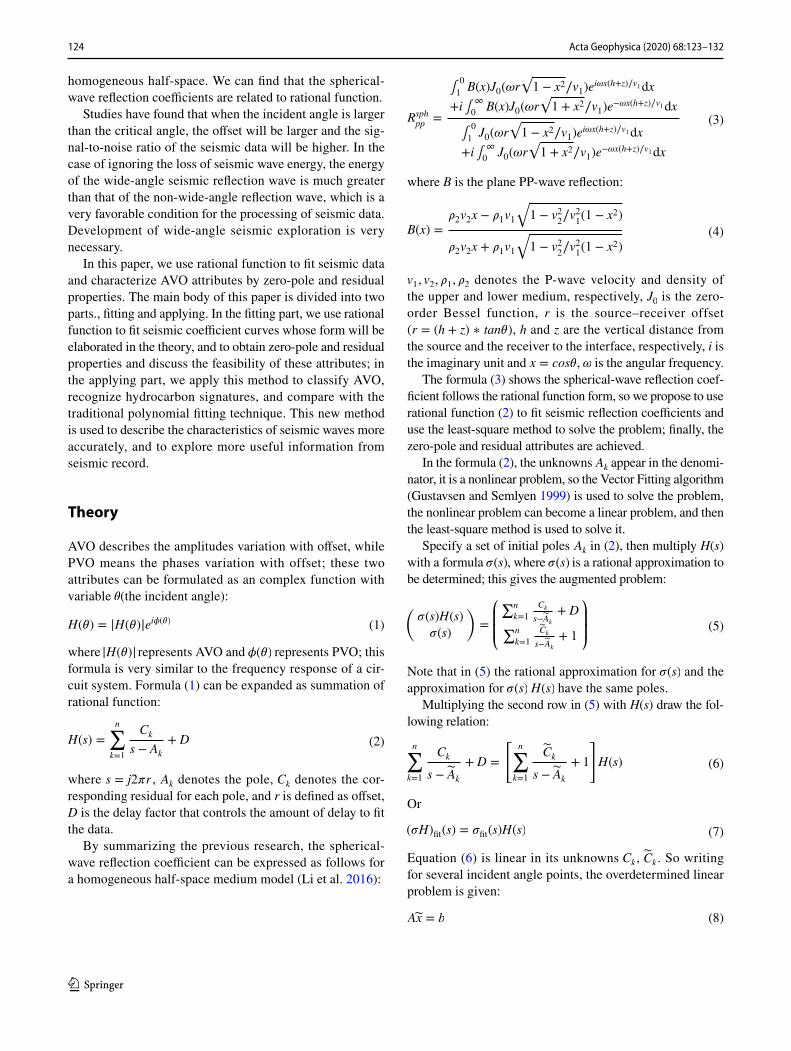
The frequency-domain AVO coefficient curve′ s ampli-tudes and phases variation with angles of model A–D are shown in Fig. 1 [each sub-figure (a) and (c)], and the fitting results are shown in the same figure. It is clear that the com-plex AVO curves are almost fitted. The poles distribution and the relative residuals are plotted in each sub-figure (b) and (d). From the results, we can see that the smaller the critical angle, the more serious the oscillation after it, and the more poles are needed to fit. Also, the curves with the larger critical angle can be fitted with less poles, so the criti-cal angle has an effect on the order of rational fitting.

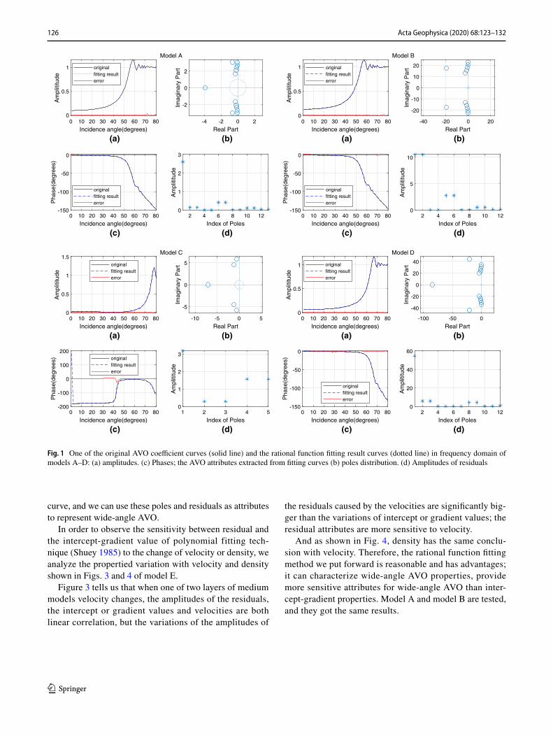
Although much more poles are needed to fit the complex AVO, the first few residuals are much more than the others, so we guess the first few residuals are the main attribute of the complex AVO. In Fig. 2 Model E (fit result), at least 12 pole and residual pairs are needed to fit the curve with the tolerance less than − 40 dB. Now the first 6 large poles and residuals are used to reconstruct the curve, and results are shown in Fig. 2 Model E (reconstruct result); it can be seen the curve reconstructed by using these 6 poles and residu-als are basically close to the original curve, and only a few oscillations after the critical angle are not fitted. So these larger poles and residuals do contain most information of the

Table 1 Parameters of AVO models (two-layer models)

Model v1∕(ms−1) �1∕(g cm−3) v2∕(ms−1) �2∕(g cm

−3)

A (avo1 gas/sand)

3093 2.40 4050 2.21

B (avo1 wet/sand)

3093 2.40 4114 2.32

C (avo2 gas/sand)

2642 2.29 2781 2.08

D (avo2 wet/sand)

2642 2.29 3048 2.23

E 2000 2.40 2933 2.20

126 Acta Geophysica (2020) 68:123–132

1 3

curve, and we can use these poles and residuals as attributes to represent wide-angle AVO.

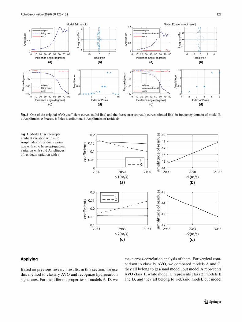
In order to observe the sensitivity between residual and the intercept-gradient value of polynomial fitting tech-nique (Shuey 1985) to the change of velocity or density, we analyze the propertied variation with velocity and density shown in Figs. 3 and 4 of model E.

Figure 3 tells us that when one of two layers of medium models velocity changes, the amplitudes of the residuals, the intercept or gradient values and velocities are both linear correlation, but the variations of the amplitudes of

the residuals caused by the velocities are significantly big-ger than the variations of intercept or gradient values; the residual attributes are more sensitive to velocity.

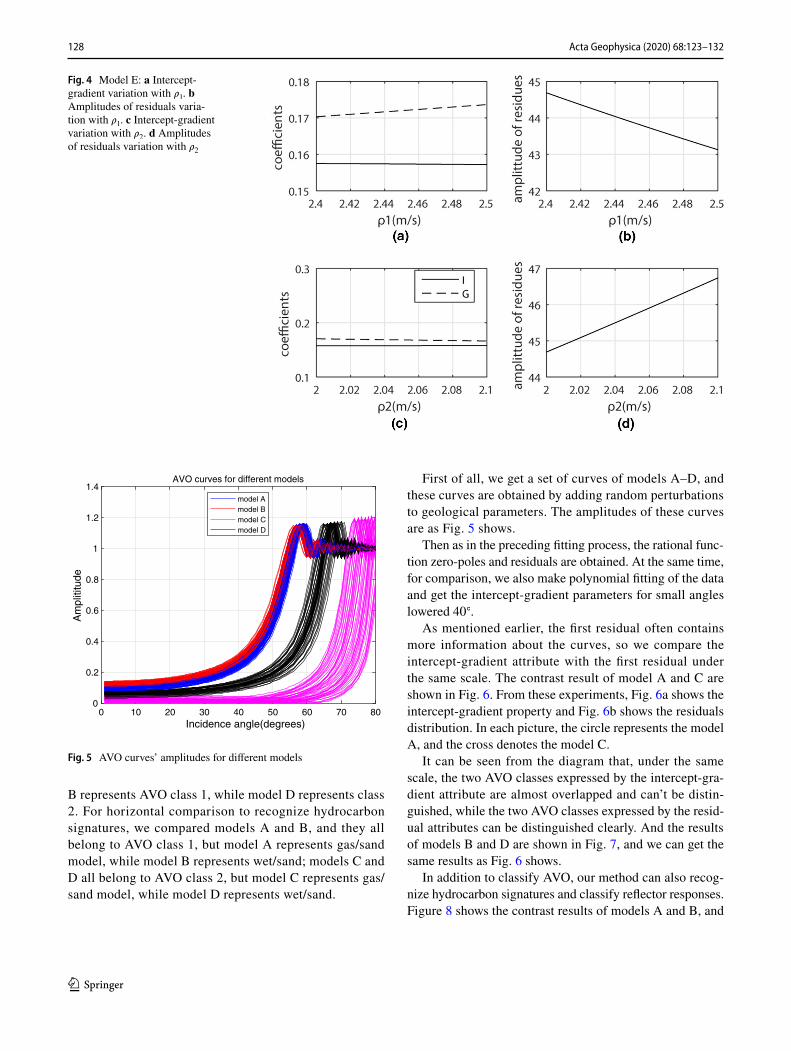
And as shown in Fig. 4, density has the same conclu-sion with velocity. Therefore, the rational function fitting method we put forward is reasonable and has advantages; it can characterize wide-angle AVO properties, provide more sensitive attributes for wide-angle AVO than inter-cept-gradient properties. Model A and model B are tested, and they got the same results.

0 10 20 30 40 50 60 70 80

Incidence angle(degrees)

(a)

0

0.5

1

Am

pliti

tude

originalfitting resulterror

0 10 20 30 40 50 60 70 80

Incidence angle(degrees)

(c)

-150

-100

-50

0

Pha

se(d

egre

es)

originalfitting resulterror

-4 -2 0 2

Real Part

(b)

-2

0

2

Imag

inar

y P

art

2 4 6 8 10 12

Index of Poles

(d)

0

1

2

3

Am

pliti

tude

Model A

0 10 20 30 40 50 60 70 80

Incidence angle(degrees)

(a)

0

0.5

1

Am

pliti

tude

originalfitting resulterror

0 10 20 30 40 50 60 70 80

Incidence angle(degrees)

(c)

-150

-100

-50

0

Pha

se(d

egre

es)

originalfitting resulterror

-40 -20 0 20

Real Part

(b)

-20

-10

0

10

20

Imag

inar

y P

art

2 4 6 8 10 12

Index of Poles

(d)

0

5

10

Am

pliti

tude

Model B

0 10 20 30 40 50 60 70 80

Incidence angle(degrees)

(a)

0

0.5

1

1.5

Am

pliti

tude

originalfitting resulterror

0 10 20 30 40 50 60 70 80

Incidence angle(degrees)

(c)

-200

-100

0

100

200

Pha

se(d

egre

es) original

fitting resulterror

-10 -5 0 5

Real Part

(b)

-5

0

5

Imag

inar

y P

art

1 2 3 4 5

Index of Poles

(d)

0

1

2

3

Am

pliti

tude

Model C

0 10 20 30 40 50 60 70 80

Incidence angle(degrees)

(a)

0

0.5

1

Am

pliti

tude

originalfitting resulterror

0 10 20 30 40 50 60 70 80

Incidence angle(degrees)

(c)

-150

-100

-50

0

Pha

se(d

egre

es)

originalfitting resulterror

-100 -50 0

Real Part

(b)

-40

-20

0

20

40

Imag

inar

y P

art

2 4 6 8 10 12

Index of Poles

(d)

0

20

40

60

Am

pliti

tude

Model D

Fig. 1 One of the original AVO coefficient curves (solid line) and the rational function fitting result curves (dotted line) in frequency domain of models A–D: (a) amplitudes. (c) Phases; the AVO attributes extracted from fitting curves (b) poles distribution. (d) Amplitudes of residuals

127Acta Geophysica (2020) 68:123–132

1 3

Applying

Based on previous research results, in this section, we use this method to classify AVO and recognize hydrocarbon signatures. For the different properties of models A–D, we

make cross-correlation analysis of them. For vertical com-parison to classify AVO, we compared models A and C, they all belong to gas/sand model, but model A represents AVO class 1, while model C represents class 2; models B and D, and they all belong to wet/sand model, but model

0 10 20 30 40 50 60 70 80

Incidence angle(degrees)

(a)

0

0.5

1

Am

pliti

tude

originalfitting resulterror

0 10 20 30 40 50 60 70 80

Incidence angle(degrees)

(c)

-150

-100

-50

0

Pha

se(d

egre

es)

originalfitting resulterror

-5 0 5

Real Part

(b)

-5

0

5

Imag

inar

y P

art

5 10 15

Index of Poles

(d)

0

0.5

1

1.5

Am

pliti

tude

Model E(fit result)

0 10 20 30 40 50 60 70 80

Incidence angle(degrees)

(a)

0

0.5

1

1.5

Am

pliti

tude

originalreconstrcut resulterror

0 10 20 30 40 50 60 70 80

Incidence angle(degrees)

(c)

-150

-100

-50

0

Pha

se(d

egre

es)

originalreconstrcut resulterror

-4 -2 0 2 4

Real Part

(b)

-2

0

2

Imag

inar

y P

art

1 2 3 4 5 6

Index of Poles

(d)

0

0.5

1

1.5

Am

pliti

tude

Model E(reconstruct result)

Fig. 2 One of the original AVO coefficient curves (solid line) and the fit/reconstruct result curves (dotted line) in frequency domain of model E: a Amplitudes. c Phases. b Poles distribution. d Amplitudes of residuals

Fig. 3 Model E: a intercept-gradient variation with v

1 . b

Amplitudes of residuals varia-tion with v

1 . c Intercept-gradient

variation with v2 . d Amplitudes

of residuals variation with v2

128 Acta Geophysica (2020) 68:123–132

1 3

B represents AVO class 1, while model D represents class 2. For horizontal comparison to recognize hydrocarbon signatures, we compared models A and B, and they all belong to AVO class 1, but model A represents gas/sand model, while model B represents wet/sand; models C and D all belong to AVO class 2, but model C represents gas/sand model, while model D represents wet/sand.

First of all, we get a set of curves of models A–D, and these curves are obtained by adding random perturbations to geological parameters. The amplitudes of these curves are as Fig. 5 shows.

Then as in the preceding fitting process, the rational func-tion zero-poles and residuals are obtained. At the same time, for comparison, we also make polynomial fitting of the data and get the intercept-gradient parameters for small angles lowered 40◦.

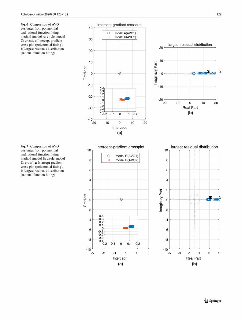
As mentioned earlier, the first residual often contains more information about the curves, so we compare the intercept-gradient attribute with the first residual under the same scale. The contrast result of model A and C are shown in Fig. 6. From these experiments, Fig. 6a shows the intercept-gradient property and Fig. 6b shows the residuals distribution. In each picture, the circle represents the model A, and the cross denotes the model C.

It can be seen from the diagram that, under the same scale, the two AVO classes expressed by the intercept-gra-dient attribute are almost overlapped and can’t be distin-guished, while the two AVO classes expressed by the resid-ual attributes can be distinguished clearly. And the results of models B and D are shown in Fig. 7, and we can get the same results as Fig. 6 shows.

In addition to classify AVO, our method can also recog-nize hydrocarbon signatures and classify reflector responses. Figure 8 shows the contrast results of models A and B, and

Fig. 4 Model E: a Intercept-gradient variation with �

1 . b

Amplitudes of residuals varia-tion with �

1 . c Intercept-gradient

variation with �2 . d Amplitudes

of residuals variation with �2

0 10 20 30 40 50 60 70 80Incidence angle(degrees)

0

0.2

0.4

0.6

0.8

1

1.2

1.4

Am

pliti

tude

AVO curves for different models

model Amodel Bmodel Cmodel D

Fig. 5 AVO curves’ amplitudes for different models

129Acta Geophysica (2020) 68:123–132

1 3

Fig. 6 Comparison of AVO attributes from polynomial and rational function fitting method (model A: circle, model C: cross). a Intercept-gradient cross-plot (polynomial fitting). b Largest residuals distribution (rational function fitting)

-20 -10 0 10 20

Intercept(a)

-40

-30

-20

-10

0

10

20

30

40

Gra

dien

t

intercept-gradient crossplot

model A(AVO1)model C(AVO2)

-0.2 -0.1 0 0.1 0.2-0.4-0.3-0.2-0.1

00.10.20.30.4

-20 -10 0 10 20

Real Part(b)

-20

-10

0

10

20

Imag

inar

y P

art

largset residual distribution

222332223322

Fig. 7 Comparison of AVO attributes from polynomial and rational function fitting method (model B: circle, model D: cross). a Intercept-gradient cross-plot (polynomial fitting). b Largest residuals distribution (rational function fitting)

Intercept

(a)

-10

-8

-6

-4

-2

0

2

4

6

8

10

Gra

dien

t

intercept-gradient crossplot

model B(AVO1)model D(AVO2)

-0.2 -0.1 0 0.1 0.2-0.4-0.3-0.2-0.1

00.10.20.30.4

-5 -3 -1 1 3 5 -5 -3 -1 1 3 5

Real Part

(b)

-10

-8

-6

-4

-2

0

2

4

6

8

10

Imag

inar

y P

art

largset residual distribution

3222222222222

130 Acta Geophysica (2020) 68:123–132

1 3

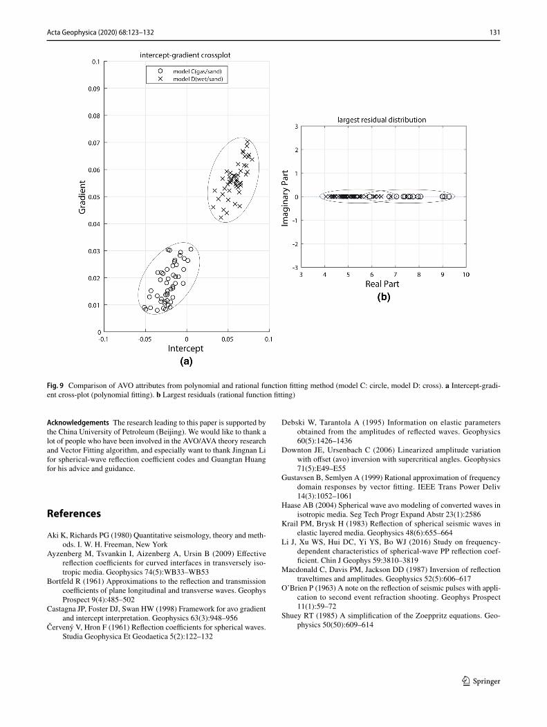
Fig. 9 shows the contrast results of models C and D. And by calculating the center distance between the AVO models, the intercept-gradient distance between the models A and B is about 0.0483 and between models C and D is about 0.0557; however, according to the zero-pole and residual characteris-tics of rational function fitting, the distance between the larg-est residuals of models A and B is about 0.1006 > 0.0483 , between models C and D is about 36.0907 > 0.0557 . There-fore, the distance calculated by our method is larger than the original polynomial fitting method, and the use of rational zero-pole and residual properties can classify reflector responses more accurately.

Conclusion

The purpose of this work is clear: to extract more useful information out of seismic data by extending the validity range of AVO analyses to larger angles. In order to achieve this goal, we have applied a new method to represent

wide-angle AVO, that is rational function fitting, based on Vector Fitting algorithm.

By doing rational function fitting to AVO curves, we obtain better approximations of wide-angle AVO and get sparse zero-pole and residual properties and thereby can improve the classification of AVO and reflector responses.

By using this method, the research range can be extended to wide-angle, and the fitting effect is ideal in large offsets. The residual properties are more sensitive to medium veloc-ity or density than intercept-gradient properties, which can be more accurately characterized AVO attributes. The limi-tation of polynomial fitting technique only in the small inci-dence angles can be improved. And under the same scale, the intercept-gradient attributes of AVO models are not easy to classify, while the zero-pole and residual attributes can be easily classified. So, the AVO or reflector responses can be classified more accurately by using rational function fit-ting than polynomial fitting. In this paper, our research is limited in the two-layer medium, and the medium analysis with more layers is our future work.

Fig. 8 Comparison of AVO attributes from polynomial and rational function fitting method (model A: circle, model B: cross). a Intercept-gradi-ent cross-plot (polynomial fitting). b Largest residuals (rational function fitting)

131Acta Geophysica (2020) 68:123–132

1 3

Acknowledgements The research leading to this paper is supported by the China University of Petroleum (Beijing). We would like to thank a lot of people who have been involved in the AVO/AVA theory research and Vector Fitting algorithm, and especially want to thank Jingnan Li for spherical-wave reflection coefficient codes and Guangtan Huang for his advice and guidance.

References

Aki K, Richards PG (1980) Quantitative seismology, theory and meth-ods. I. W. H. Freeman, New York

Ayzenberg M, Tsvankin I, Aizenberg A, Ursin B (2009) Effective reflection coefficients for curved interfaces in transversely iso-tropic media. Geophysics 74(5):WB33–WB53

Bortfeld R (1961) Approximations to the reflection and transmission coefficients of plane longitudinal and transverse waves. Geophys Prospect 9(4):485–502

Castagna JP, Foster DJ, Swan HW (1998) Framework for avo gradient and intercept interpretation. Geophysics 63(3):948–956

Červený V, Hron F (1961) Reflection coefficients for spherical waves. Studia Geophysica Et Geodaetica 5(2):122–132

Debski W, Tarantola A (1995) Information on elastic parameters obtained from the amplitudes of reflected waves. Geophysics 60(5):1426–1436

Downton JE, Ursenbach C (2006) Linearized amplitude variation with offset (avo) inversion with supercritical angles. Geophysics 71(5):E49–E55

Gustavsen B, Semlyen A (1999) Rational approximation of frequency domain responses by vector fitting. IEEE Trans Power Deliv 14(3):1052–1061

Haase AB (2004) Spherical wave avo modeling of converted waves in isotropic media. Seg Tech Progr Expand Abstr 23(1):2586

Krail PM, Brysk H (1983) Reflection of spherical seismic waves in elastic layered media. Geophysics 48(6):655–664

Li J, Xu WS, Hui DC, Yi YS, Bo WJ (2016) Study on frequency-dependent characteristics of spherical-wave PP reflection coef-ficient. Chin J Geophys 59:3810–3819

Macdonald C, Davis PM, Jackson DD (1987) Inversion of reflection traveltimes and amplitudes. Geophysics 52(5):606–617

O’Brien P (1963) A note on the reflection of seismic pulses with appli-cation to second event refraction shooting. Geophys Prospect 11(1):59–72

Shuey RT (1985) A simplification of the Zoeppritz equations. Geo-physics 50(50):609–614

Fig. 9 Comparison of AVO attributes from polynomial and rational function fitting method (model C: circle, model D: cross). a Intercept-gradi-ent cross-plot (polynomial fitting). b Largest residuals (rational function fitting)

132 Acta Geophysica (2020) 68:123–132

1 3

Ursenbach C, Haase AB, Downton JE (1949) An efficient method for avo modeling of reflected spherical waves. Seg Tech Progr Expand Abstr 24(1):202–205

Winterstein DF (1985) Supercritical reflections observed in p- and s- wave data. Geophysics 50(2):185

Zhu X, Mcmechan GA (2015) Elastic inversion of near- and post-critical reflections using phase variation with angle. Geophysics 77(4):149