Embed Size (px)
Citation preview
Novel Predistortion Techniques for RF Power Amplifiers
Ming Xiao
A thesis submitted to
The University of Birmingham
for the degree of
DOCTOR OF PHILOSOPHY
School of Electronic, Electrical
and Computer Engineering
The University of Birmingham
October, 2009

University of Birmingham Research Archive
e-theses repository This unpublished thesis/dissertation is copyright of the author and/or third parties. The intellectual property rights of the author or third parties in respect of this work are as defined by The Copyright Designs and Patents Act 1988 or as modified by any successor legislation. Any use made of information contained in this thesis/dissertation must be in accordance with that legislation and must be properly acknowledged. Further distribution or reproduction in any format is prohibited without the permission of the copyright holder.

ABSTRACT
As the mobile phone is an essential accessory for everyone nowadays, predistortion
for the RF power amplifiers in mobile phone systems becomes more and more
popular. Especially, new predistortions for power amplifiers with both nonlinearities
and memory effects interest the researchers. In our thesis, novel predistortion
techniques are presented for this purpose. Firstly, we improve the digital injection
predistortion in the frequency domain. Secondly, we are the first authors to propose a
novel predistortion, which combines digital LUT (Look-up Table) and injection.
These techniques are applied to both two-tone tests and 16 QAM (Quadrature
Amplitude Modulation) signals. The test power amplifiers vary from class A, inverse
class E, to cascaded amplifier systems.
Our experiments have demonstrated that these new predistortion techniques can
reduce the upper and lower sideband third order intermodulation products in a
two-tone test by 60 dB, or suppress the spectral regrowth by 40 dB and reduce the
EVM (Error Vector Magnitude) down to 0.7% rms in 16 QAM signals, disregarding
whether the tested power amplifiers or cascade amplifier systems exhibit significant
nonlinearities and memory effects.
i

ACKNOWLEDGEMENTS
The research would not have been possible without my supervisor, Dr Peter Gardner. I
would like to take this opportunity to thank him for his encouragement, advice and all
the supports including academic and non-academic. The internal assessor, Prof. Hall,
provided helpful comments for my PhD reports. Research fellow, Mury Thian, gave
suggestions on my papers. Other members of the Communication Engineering
research group and the department, who contributed in various helps such as lab
equipment set up (Allan Yates) and computer installation (Gareth Webb). Dr Steven
Quigley and Dr Sridhar Pammu, gave useful advice and support on FPGA broad.
There are some people who did not contribute to the work itself, but supported me
during the work, my parents, my girl friend, Jian Chen, and my friends, Zhen Hua Hu,
Qing Liu, Jin Tang, and Kelvin.
Finally I acknowledge my financial support provided by the Engineering and Physical
Sciences Research Council.
ii

ABBREVIATIONS ACPR Adjacent Channel Power Ratio ADC Analog-to-Digital Converter AM Amplitude Modulation ANFIS Adaptive Neuro-Fuzzy Inference System ANN Artificial Neural Network ARMA Auto-Regressive Moving Average filter BP Back Propagation BPF Band Pass Filter CDMA Code Division Multiple Access CMOS Complementary Metal Oxide Semiconductor DAC Digital-to-Analog Converter DC Direct Current DECT Digital Enhanced Cordless Telecommunications DSP Digital Signal Processing/Processor DUT Device Under Test EDET Envelope DETector EPD Envelope PreDistorter EVM Error Vector Magnitude FIR Finite Impulse Response FIS Fuzzy Inference System FPGA Field Programmable Gate Array GPS Global Positioning System GSM Global System for Mobile communication IC Integrated Circuit IF Intermediate Frequency IIR Infinite Impulse-Response IM3 Third -order InterModulation IM3L Lower Third-order InterModulation product IM3U Upper Third-order InterModulation product LTI Linear Time Invariant LUT Look-Up Table L+I Look-up table plus Injection PA Power Amplifier PC Personal Computer
iii

PD PreDistorter PLL Phase Lock Loop PM Phase Modulation QAM Quadrature Amplitude Modulation QPSK Quadrature Phase-Shift Keying RF Radio Frequency TWT Traveling Wave Tube UMTS Universal Mobile Telecommunications System VMOD Vector MODulator VSA Vector Signal Analyzer WLAN Wireless Local Area Network
iv

CONTENTS
Chapter 1 Introduction ………………………………………………...... 1
1.1 Power efficiency, linearity and linearization …………………………………….. 1
1.2 Analogue linearization …………………………………………………………… 3
1.2.1 Feedback …………………………………………………………………….. 3
1.2.2 Feed forward ………………………………………………………………... 4
1.2.3 Limitation of these techniques ……………………………………………… 5
1.3 digital predistortion for linearization …………………………………………….. 5
1.4 Scope of the thesis ……………………………………………………………….. 7
Chapter 2 Background ………………………………………... 8
2.1 Power amplifier modeling ……………………………………………………….. 8
2.1.1 Memoryless nonlinear power amplifier model ……………………………... 8
2.1.1.1 AM/AM and AM/PM conversion ………………………………………. 8
2.1.1.2 Memoryless polynomial model ……………………………………….. 10
2.1.1.3 Saleh model (frequency-independent) ………………………………….12
2.1.2 Memory effects …………………………………………………………….. 13
2.1.3 Nonlinear with memory effect power amplifier model ……………………. 14
2.1.3.1 Frequency-dependant nonlinear quadrature model …………………… 14
2.1.3.2 Clark’s ARMA model …………………………………………………. 16
2.1.3.3 Volterra series …………………………………………………………. 17
2.1.3.4 Neural network based model ………………………………………….. 21
2.2 Predistortion for power amplifier ………………………………………………. 21
2.2.1 AM/AM and AM/PM conversion ………………………………………….. 22
2.2.2 Adjacent channel emissions ……………………………………………….. 25
v

2.2.3 Inverse Volterra model …………………………………………………….. 26
2.2.3.1 Inverse memory polynomial model……...…………………………….. 27
2.2.3.2 Hammerstein model …………………………………………………... 28
2.2.4 Computational method …………………………………………………….. 29
2.2.4.1 Neural network ………………………………………………………... 30
2.2.4.2 Fuzzy system and Fuzzy inference system ……………………………. 31
2.2.4.3 Neuro-Fuzzy system …………………………………………………... 33
2.2.4.4 ANFIS predistortion …………………………………………………... 35
2.2.5 Injection predistortion ……………………………………………………... 36
2.2.5.1 Injection in two-tone test …………………………………………….... 36
2.2.5.2 Injection in wideband signals …………………………………………. 39
2.3 Summary ……………………………………………………………………….. 41
Chapter 3 Improvements of Injection Techniques in two-tone
Test ………………………………………………………...… 44
3.1 Introductions of two-tone tests …………………………………………………. 44
3.2 Published measurements and injections for IM3 products in two-tone tests …... 47
3.2.1 Measurements on IM3 products …………………………………………… 48
3.2.2. Injections on IM3 products ……………………………………………….. 51
3.3 Improvements for the measurements and injections in two-tone tests …………. 51
3.3.1 IM3 reference ……………………………………………………………… 53
3.3.1.1 Experimental setup ……………………………………………………. 54
3.3.1.2 Data organization ……………………………………………………... 54
3.3.1.3 Test details …………………………………………………………….. 56
3.3.1.4 Theory and experimental analysis for IM3 reference ………………… 56
3.3.1.5 IM3 measurement and results …………………………………………. 58
3.3.2 Model for single sideband injection ……………………………………..… 60
3.3.3 Interaction and dual sideband predistortion ……………………………….. 63
vi
3.3.3.1 Interaction ……………………………………………………………... 64
3.3.3.2 Dual sideband predistortion …………………………………………... 67
3.3.4 Improvement by iteration ………………………………………………….. 69
3.3.4.1 Reasons for iteration …………………………………………………... 69
3.3.4.2 Iteration algorithm and feasibility …………………………………….. 71
3.3.4.3 Experimental results …………………………………………………... 72
3.3.5 Injection predistortion in different signal conditions ……………………… 74
3.4 Summary ……………………………………………………………………….. 76
Chapter 4 Application of Injection Predistortion Techniques in
16 QAM Signals …………………………………………….. 78
4.1 Published injection predistortion result for wideband signal …………………... 78
4.2 Proposed digital baseband injection ……………………………………………. 80
4.2.1 Experimental setup ………………………………………………………… 80
4.2.2 Sub-frequency allocation and calculation ..…………..……………………. 82
4.2.3 Experimental results ……………………………………………………….. 91
4.3 Summary ……………………………………………………………………….. 92
Chapter 5 Combine LUT plus Injection Predistortion ………. 94
5.1 Mathematical relations between LUT and injection …………………………… 94
5.2 Experimental comparisons between LUT and injection ……………………..… 97
5.3 L+I predistorter ……………………………………………………………….. 101
5.3.1 Basic idea of L+I …………………………………………………………. 101
5.3.2 Experimental PA system and comparison results ……………………........ 102
5.4 Summary ……………………………………………………………………… 106
vii

Chapter 6 Summary and Conclusion …………………….… 107
6.1 Summary ……………………………………………………………………… 107
6.2 Major contributions and achievements ……………………………………….. 110
6.3 Suggestions for future work …………………………………………………... 111
6.4 Conclusions …………………………………………………………………… 113
Reference …………………………………………………... 114
Appendix A ………………………………………………… 119
Appendix B ……………………………………………….... 120
Appendix C ………………………………………………… 121
Appendix D ………………………………………………… 122
Appendix E ………………………………………………… 136
Appendix F ………………………………………………… 144
Appendix G ………………………………………………… 148
Published Papers
viii
FIGURES
1-1 Power amplifier linearization scheme …………………………………..……….. 2
1-2 General feedback structure ………………………………………………………. 3
1-3 Feed forward linearization ………………………………………………………. 4
1-4 Schematic of an amplifier and its predistorter …………………………………... 6
2-1 AM/AM conversion ……………………………………………...……………… 9
2-2 AM/PM conversion …………………………………………………………….. 10
2-3 Two-tone test output spectrum close to carriers ………………………………... 12
2-4 Quadrature nonlinear model of PA ……………………………………………... 13
2-5 Saleh’s frequency-dependent model of a TWT amplifier ……………………… 15
2-6 Abuelma’Atti’s frequency-dependant Quadrature model ……………………… 16
2-7 Nonlinear ARAM model of PA ………………………………………………… 17
2-8 Parallel Wiener model ………………………………………………………….. 18
2-9 Memory polynomial model with sparse delay taps ……………………………. 20
2-10 Time-delay neural network for PA model …………………………………….. 21
2-11 Predistorter proposed in [20] ………………………………………………….. 22
2-12 Envelope linearization ………………………………………………………… 23
2-13 PDPA module …………………………………………………………………. 23
2-14 RF envelope predistortion system ……………………………………………. 24
2-15 Combine digital/analogue cooperation predistortion …………………………. 24
2-16 Predistorter proposed in [24] …………………………………………………. 25
2-17 Relation between Volterra model and its PA/PD model ……………………… 26
2-18 Indirect learning architecture for the predistorter ………………………..…… 27
2-19 Hammerstein predistorter in indirect learning architecture …………………... 28
2-20 Augmented Hammerstein predistorter ………………………………………... 29
2-21 A simple neural network example …………………………………………….. 30
2-22 Sigmoid function ……………………………………………………………… 31
ix
2-23 Sugeno fuzzy model …………………………………………………………... 33
2-24 Equivalent ANFIS for Sugeno fuzzy model ………………………………….. 34
2-25 ANFIS for predistortion ………………………………………………………. 35
2-26 Basic idea of correction ……………………………………………………….. 37
2-27 Injection predistorter ………………………………………………………….. 41
3-1 A two-tone test signal ………………………………………………………….. 46
3-2 IM3 phase measurement in [56] ……………………………………………….. 48
3-3 IM3 phase measurement in [59] ……………………………………………….. 49
3-4 IM3 phase measurement in [60] ……………………………………………….. 50
3-5 IM3 phase measurement in [41] ……………………………………………….. 51
3-6 Experimental set up ……………………………………………………………. 54
3-7 Measured IM3 amplitudes and phases
(a) Measured amplitudes of IM3L ……………………………………………… 59
(b) Measured phase distortion of IM3L ……………………………………...… 59
(c) Measured amplitudes of IM3U ……………………………………………... 59
(d) Measured phases distortion of IM3U ………………………………………. 59
3-8 Plots of Rlower …………………………………………………………………… 61
3-9 (a) Two-tone test ……………………………………………………………….. 63
(b) Lower Sideband Injection ………………………………………………...… 63
(c) Upper Sideband Injection …………………………………………………... 63
3-10 Injection without considering interactions ………………………………….… 64
3-11 Plots of Rlower-upper ……………………………………………………………... 66
3-12 Measured dual sideband injection predistortion considering interactions .…… 69
3-13 Variation of radius with angle from Fig. 3-8 …………………………………. 70
3-14 (a) Lower sideband injection with 2 iterations ………………………………... 73
(b) Upper sideband injection with 2 iterations ………………………………... 73
(c) Dual sideband injection without considering interactions ………………… 74
(d) Dual sideband injection considering interactions with 2 iterations ……….. 74
3-15 (a) IM3s power level before/after injection …………………………………... 75
x

(b) Amplitude of injected IM3s ……………………………………………….. 76
(c) Angle of injected IM3s ……………………………………………………. 76
4-1 Second harmonic injection in wideband signal in [48] ………………………… 79
4-2 Third- and fifth-order injection in W-CDMA in [51] …………………………... 79
4-3 Simultaneous harmonic and baseband signal injection [47] …………………… 80
4-4 Experimental setup ……….…………………………………………………….. 82
4-5 (a) Measured output spectrum of a 16 QAM signal …………………………… 82
(b) Measured (normalized) and ideal constellation ………………………..…… 83
4-6 (a) Amplitude of 16 QAM signals and injection ……………………………….. 85
(b) Phase of 10 different injections …………………………………………….. 85
4-7 Input spectrum of injection …………………………………………………….. 86
4-8 Sub-frequency from 51 to 55 …………………………………………………... 87
4-9 Ideal input output relation for each sub-frequency …………………………….. 87
4-10 Flowchart for iterative computation of injection in 16 QAM ………………… 89
4-11 Output spectra in injection predistortion ……………………………………… 91
4-12 Upper sideband injection ……………………………………………………... 92
5-1 Digital predistortion for a power amplifier …………………………………….. 94
5-2 Explanation of linear gain back-off in LUT ……………………………………. 95
5-3 Normalized AM/AM and AM/PM measurement ………………………………. 97
5-4 IM3 asymmetries at different two-tone input power …………………………... 97
5-5 Comparison of power spectra ………………………………………………….. 98
5-6 Comparison on EVM …………………………………………………………... 98
5-7 Comparison of output constellations …………………………………………... 99
5-8 L+I predistorter ……………………………………………………………….. 102
5-9 Normalized AM/AM, AM/PM measurements ………………………………... 102
5-10 IM3 asymmetries at different two-tone input powers ……………………….. 103
5-11 Comparison of power spectra ……………………………………………..… 103
5-12 Comparison on EVM ………………………………………………………... 104
xi

5-13 Comparison of output constellations ………………………………………... 104
5-14 Application of L+I in an Inverse Class E PA ………………………………... 106
xii

TABLES
2-1 Two-tone intermodulation products up to fifth order …………………………... 11
4-1 Values for K ……………………………………………………………………. 84
5-1Experimental Measurements ……………………………………………………. 99
5-2 Experimental Measurements ………………………………………………….. 105
6-1 FPGA pipeline ………………………………………………………………… 111
xiii

CHAPTER 1
INTRODUCTION Nowadays, the mobile phone is an essential accessory for everyone. Thus, researchers
and engineers in communication technology are exploring new devices for wireless
transceivers for the demanded market. The power amplifier is the key component in
the transmitter. For a power amplifier, high power efficiency is a basic requirement
because of the energy issue. At the same time, high linearity is more and more
desirable today, to minimize the frequency interference and allow higher transmission
capacity in wideband communication systems. The more linear the transmitters, the
more user channels can be fitted in to the available spectrum. Particularly with the
trend of mobile phone technology moving towards multi-band and multi-mode
systems, where different wireless communication standards such as global positioning
system (GPS), digital enhanced cordless telecommunications (DECT), global system
for mobile communications (GSM), universal mobile telecommunications system
(UMTS), Bluetooth and wireless local area network (WLAN) are to be integrated
altogether. Power amplifiers with both excellent linearity and high power efficiency
are increasingly essential in the transmitters. However, it is well known that high
linearity will sacrifice the power efficiency in power amplifiers. The only solution for
this problem is linearization. As a result, linearization techniques which allow power
amplifiers to have both high power efficiency and high linearity, interest the
researchers.
1.1 Power efficiency, linearity and linearization
All power amplifiers have nonlinear properties, which become dominant in their
saturation range. On the other hand, the maximum power efficiency generally occurs
1
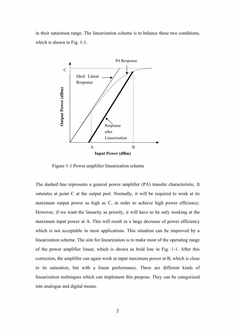
in their saturation range. The linearization scheme is to balance these two conditions,
which is shown in Fig. 1-1.
Out
put P
ower
(dB
m)
Input Power (dBm) A B
Response after Linearization
PA Response
Ideal Linear Response
C
Figure 1-1 Power amplifier linearization scheme
he dashed line represents a general power amplifier (PA) transfer characteristic. It T
saturates at point C at the output port. Normally, it will be required to work at its
maximum output power as high as C, in order to achieve high power efficiency.
However, if we want the linearity as priority, it will have to be only working at the
maximum input power at A. This will result in a large decrease of power efficiency
which is not acceptable in most applications. This situation can be improved by a
linearization scheme. The aim for linearization is to make most of the operating range
of the power amplifier linear, which is shown as bold line in Fig. 1-1. After this
correction, the amplifier can again work at input maximum power at B, which is close
to its saturation, but with a linear performance. There are different kinds of
linearization techniques which can implement this purpose. They can be categorized
into analogue and digital means.
2

1.2 Analogue linearization
1.2.1 Feedback
The basic structure of feedback circuit is shown in Fig. 1-2.
A y(t)
-1/K
d(t)
x(t)
Figure 1-2 General feedback structure
In this structure, the input signal is x(t), the gain of the PA is A, the gain of the
feedback loop is -1/K, and the distortion is d(t) which is added after the gain of the PA.
The output can be obtained directly as:
( ) ( ) ( )tdKA
KtxAK
AKty+
++
= (1.1)
If we assume that the amplifier gain is much greater than the feedback loop gain, i.e.,
A>>K, (1.1) can be simplified to:
( ) ( ) ( )tdAKtKxty += (1.2)
From (1.2), we can see that the gain of the signal is lowered from A down to K, and
3

the distortion will be significantly reduced by K/A.
A typical feedback loop for linearization techniques is Cartesian feedback, further
detail can be found in [1].
1.2.2 Feed forward
Fig. 1-3 shows a feed forward linearization scheme [2].
Figure 1-3 Feed forward linearization
In the lower branch of the circuit, a sample of the input is subtracted from a sample of
output of the main amplifier, to generate an error signal, or intermodulation products
in the spectral domain. This error signal is amplified though an error amplifier, to
have the same amplitude as the output error of the main amplifier. A time delay line is
inserted between the two couplers in the upper branch, which make the errors from
the two branches have 180 degree phase difference. The errors cancel each other in
the last coupler, making the output linear again.
4

1.2.3 Limitation of these techniques
In the feedback predistortion, the output signal goes back to the subtractor through the
feedback loop. This will take a certain time. When considering this delay of the
feedback loop, the overall equation is:
( ) ( ) ( )tdttyKAtAxty +Δ−−= )( (1.3)
where ∆t denotes the delay of the feedback loop. It is only when y(t) is equal or near
to y(t-∆t), that (1.3) can equal to (1.1). In RF field, a small time delay can cause a
great phase shift. Hence, the difference between y(t) and y(t-∆t) can be significant and
fatal in an RF transmitter.
On the other hand, the feed forward technique has a power efficiency problem. The
lower branch amplifier consumes a certain power. However, this output does not
make a positive contribution, but a subtraction from the output of main amplifier.
From the point of view of power, the error amplifier is making extravagant
consumption. Practically, this kind of linearization (i.e. Feed forward) has 20% of
power efficiency at best. This compares poorly with other linearization schemes such
as predistortion, where efficiencies greater than 50% can be achieved.
1.3 Digital predistortion for linearization
Besides analogue linearization, there are different kinds of digital predistortion
techniques. The basic idea is shown in Fig. 1-4.
5
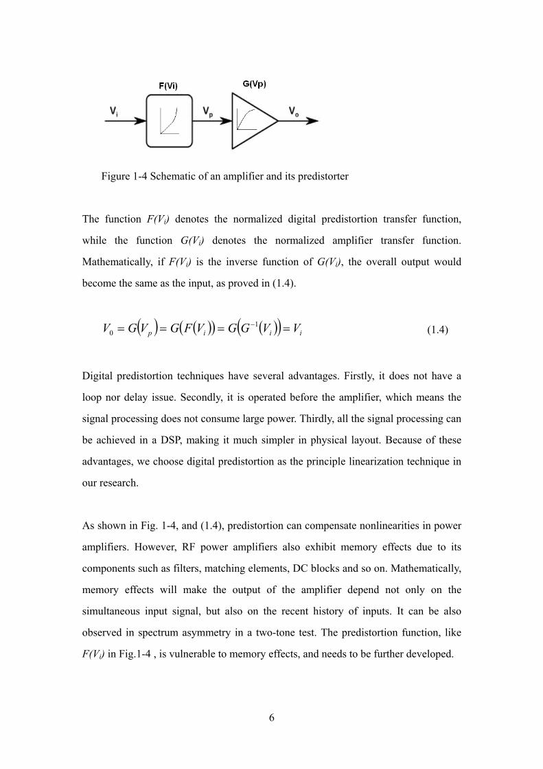
Figure 1-4 Schematic of an amplifier and its predistorter
The function F(Vi) denotes the normalized digital predistortion transfer function,
while the function G(Vi) denotes the normalized amplifier transfer function.
Mathematically, if F(Vi) is the inverse function of G(Vi), the overall output would
become the same as the input, as proved in (1.4).
( ) ( )( ) ( )( ) iiip VVGGVFGVGV ==== −10 (1.4)
Digital predistortion techniques have several advantages. Firstly, it does not have a
loop nor delay issue. Secondly, it is operated before the amplifier, which means the
signal processing does not consume large power. Thirdly, all the signal processing can
be achieved in a DSP, making it much simpler in physical layout. Because of these
advantages, we choose digital predistortion as the principle linearization technique in
our research.
As shown in Fig. 1-4, and (1.4), predistortion can compensate nonlinearities in power
amplifiers. However, RF power amplifiers also exhibit memory effects due to its
components such as filters, matching elements, DC blocks and so on. Mathematically,
memory effects will make the output of the amplifier depend not only on the
simultaneous input signal, but also on the recent history of inputs. It can be also
observed in spectrum asymmetry in a two-tone test. The predistortion function, like
F(Vi) in Fig.1-4 , is vulnerable to memory effects, and needs to be further developed.
6
1.4 Scope of the thesis
This thesis investigates and implements published and novel techniques in digital
predistortion linearization. The organization of this thesis is as follows:
Since the ideal digital predistorter is the inverse function of the power amplifier’s
transfer characteristic, Chapter 2 will firstly review published models which describe
the nonlinearities for the power amplifiers, and then their inverse models which
perform as predistorters. Meanwhile, we will explore memory effects as well, which
decrease the results of these digital linearization techniques. Further, we will
introduce another digital predistortion technique named injection. We will analyze its
mechanism and compare it with conventional digital predistortion.
After examining published injection techniques, we present our injection technique in
Chapter 3 and 4. Chapter 3 will focus on its application in two-tone tests, while
Chapter 4 will focus on 16 QAM wideband signals. In these two chapters, we will
fully explore this injection technique, including its advantages, technical problems
existing in related published work and our solutions. Hence, our novel injection yields
further improvements in terms of intermodulation reductions in two-tone test cases
and spectral regrowth reductions in wideband signal cases.
This new injection technique is firstly combined with LUT predistortion in Chapter 5.
The aim is to make this new predistortion (L+I) inherit the advantages from LUT and
injection. The overall performance is better than any single technique, in terms of
adjacent channel power ratio (ACPR) and error vector magnitude (EVM) reduction.
This has been demonstrated with a cascaded PA system which shows both significant
nonlinearities and memory effects.
7

CHAPTER 2
BACKGROUND This chapter generally outlines several published models of power amplifiers and
predistorters.
2.1 Power amplifier modeling
The objective of linearization is to produce highly linear power amplifiers.
Specifically, a perfect predistorter is an inverse model of the power amplifier. As a
result, to explore various PA models is the priority of the research. The PA models can
be divided into two general categories. One is the memoryless nonlinear model and
the other is nonlinear with memory effect model [2].
2.1.1 Memoryless nonlinear power amplifier model
This kind of model only describes the nonlinearities that exist in the PA. In other
words, in a two-tone test, the intermodulation products do not depend on the
frequencies and tone spacing of the carriers. This kind of model is suitable to describe
the PA response for single sine waves and narrow bandwidth signals.
2.1.1.1 AM/AM and AM/PM conversion
AM/AM and AM/PM conversion provide the basis for a well-know memoryless PA
model. AM/AM describes the relationship between input power and output power,
8
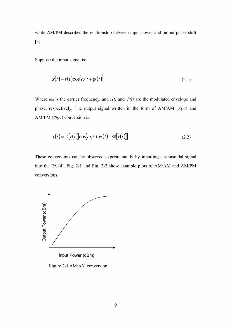
while AM/PM describes the relationship between input power and output phase shift
[3].
Suppose the input signal is:
( ) ( ) ( )[ tttrtx ]ψω += 0cos (2.1)
Where ω0 is the carrier frequency, and r(t) and Ψ(t) are the modulated envelope and
phase, respectively. The output signal written in the form of AM/AM (A(r)) and
AM/PM (Φ(r)) conversion is:
( ) ( )[ ] ( ) ( )[ ][ trtttrAty ]Φ++= ψω0cos (2.2)
These conversions can be observed experimentally by inputting a sinusoidal signal
into the PA [4]. Fig. 2-1 and Fig. 2-2 show example plots of AM/AM and AM/PM
conversions.
Input Power (dBm)
Out
put P
ower
(dBm
)
Figure 2-1 AM/AM conversion
9

Out
put P
hase
Dis
torti
on (d
egre
e)
Input Power (dBm)
Figure 2-2 AM/PM conversion
2.1.1.2 Memoryless polynomial model
The input-output relation of a memoryless PA can be written in the form of a
polynomial:
...55
44
33
221 +++++= xaxaxaxaxay (2.3)
where x and y represent the input and output signal, and a are complex coefficients.
This model can calculate the two-tone test simply. If a two-tone signal is:
( ) ( ) ( )tVtVtx 21 coscos ωω += (2.4)
We substitute (2.4) into (2.3), and get:
( ) ( ) ( )[ ] ( ) ( )[ ]( ) ( )[ ] ( ) ( )[( ) ( )[ ] ...coscos
coscoscoscos
coscoscoscos
521
55
421
44
321
33
221
22211
+++
++++
+++=
ttVa
ttVattVa
ttVattVaty
ωω
ωωωω
ωωωω
] (2.5)
10

All the resulting harmonic and intermodulation products are listed in Table 2-1.
Order Terms a1V a2V2 a3V3 a4V4 a5V5
Zero DC 1 9/4
ω1 1 9/4 25/4 First
ω2 1 9/4 25/4
2ω1 1/2 2
2ω2 1/2 2
Second
ω1±ω2 1 3
3ω1 1/4 25/16
3ω2 1/4 25/16
2ω1±ω2 3/4 25/8
Third
2ω2±ω1 3/4 25/8
4ω12 1/8
4ω2 1/8
3ω1±ω2 1/2
3ω2±ω1 1/2
Fourth
2ω1±ω 3/4
5ω1 1/16
5ω2 1/16
4ω1±ω2 5/16
4ω2±ω1 5/16
3ω1±2ω2 5/8
Fifth
3ω2±2ω1 5/8
Table 2-1 Two-tone intermodulation products up to fifth order
In narrow band systems, the even-order products cause less concern than the
odd-order products, since they are out of band and can be filtered out easily. The
two-tone test output spectrum close to the carriers is shown in Fig. 2-3.
11
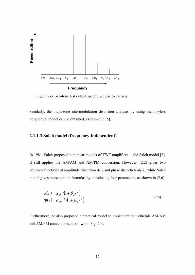
Figure 2-3 Two-tone test output spectrum close to carriers
Similarly, the multi-tone intermodulation distortion analysis by using memoryless
polynomial model can be obtained, as shown in [5].
2.1.1.3 Saleh model (frequency-independent)
In 1981, Saleh proposed nonlinear models of TWT amplifiers— the Saleh model [6].
It still applies the AM/AM and AM/PM conversion. However, (2.2) gives two
arbitrary functions of amplitude distortion A(r) and phase distortion Φ(r) , while Saleh
model gives more explicit formulas by introducing four parameters, as shown in (2.6).
( ) ( )( ) ( 22
2
1/
1/
rrr
rrrA aa
ΦΦ +=Φ
+=
βα
βα
) (2.6)
Furthermore, he also proposed a practical model to implement the principle AM/AM
and AM/PM conversions, as shown in Fig. 2-4.
12

( ) ( ) ( )( )ttrPtp ψω += 0cos
Figure 2-4 Quadrature nonlinear model of PA in [6]
Fig.2-4: In
( ) ( ) ([ ]( ) ( ) ( )[ ]rrArQ
rrArPΦ=Φ=
sincos )
(2.7)
uppose the input is the same as (2.1), this model will give the output of:
Φ++=+Φ−+Φ=
+−+=+=
ψωψωψω
ψωψω
0
00
00
cossinsincoscos
sincos)(
(2.8)
hich is the same as (2.2).
2.1.2 Memory effects
ory effects cause the amplitude and phase of distortion components to vary with
S
( ) ( )( ) ( )[ ] ( ) ( )[ ]( ) ( )[ ] ( )[ ] ( ) ( )[ ] ( )[ ]( ) ( ) ( )[ ]rttrA
ttrrAttrrAttrQttrP
tqtpty
w
Mem
the modulation frequency [7] , hence generating asymmetry between intermodulation
products.
90o Q(r)
P(r)
( ) ( ) ( )( )tttrtx ψω += 0cos
( ) ( ) ( )( )ttrQtq ψω +0sin
( ) ( ) ( )tqtpty +=
= −
13

Take the third order intermodulation products (IM3) for example. In a memoryless PA,
according to Table 2-1, the lower and upper sideband IM3 levels are:
334
33 VaIM = (2.9)
Equation (2.9) shows that IM3 is not a function of tone spacing and that the upper and
lower IM3 should have the same magnitude. But in some cases [8, 9], these IM3s are
asymmetric, and their ratio changes as the tone spacing varies, and this is caused by
memory effects.
Memory effects can have thermal or electrical origins. Thermal memory effects are
caused by electro-thermal couplings, while electrical memory effects [10] are caused
by the way the impedances seen by the baseband, fundamental and harmonic signal
components vary with the modulation frequency. Both of these memory effects can
affect modulation frequencies up to a few megahertz. As a result, PA models
considering memory effects are more practical in wideband communication.
2.1.3 Nonlinear with memory effect power amplifier model
Different from the memoryless model, these models describe both of the
nonlinearities and memory effects that exist in PAs.
2.1.3.1 Frequency-dependent nonlinear quadrature model
Saleh also proposed a frequency-dependent model in [6], which is shown in Fig.2-5.
14
90o Hq(f)
( )tx ( )ty
Qo(r) Gq(f)
P(r,f)
Q(r,f)
Hp(f) Po(r) Gp(f)
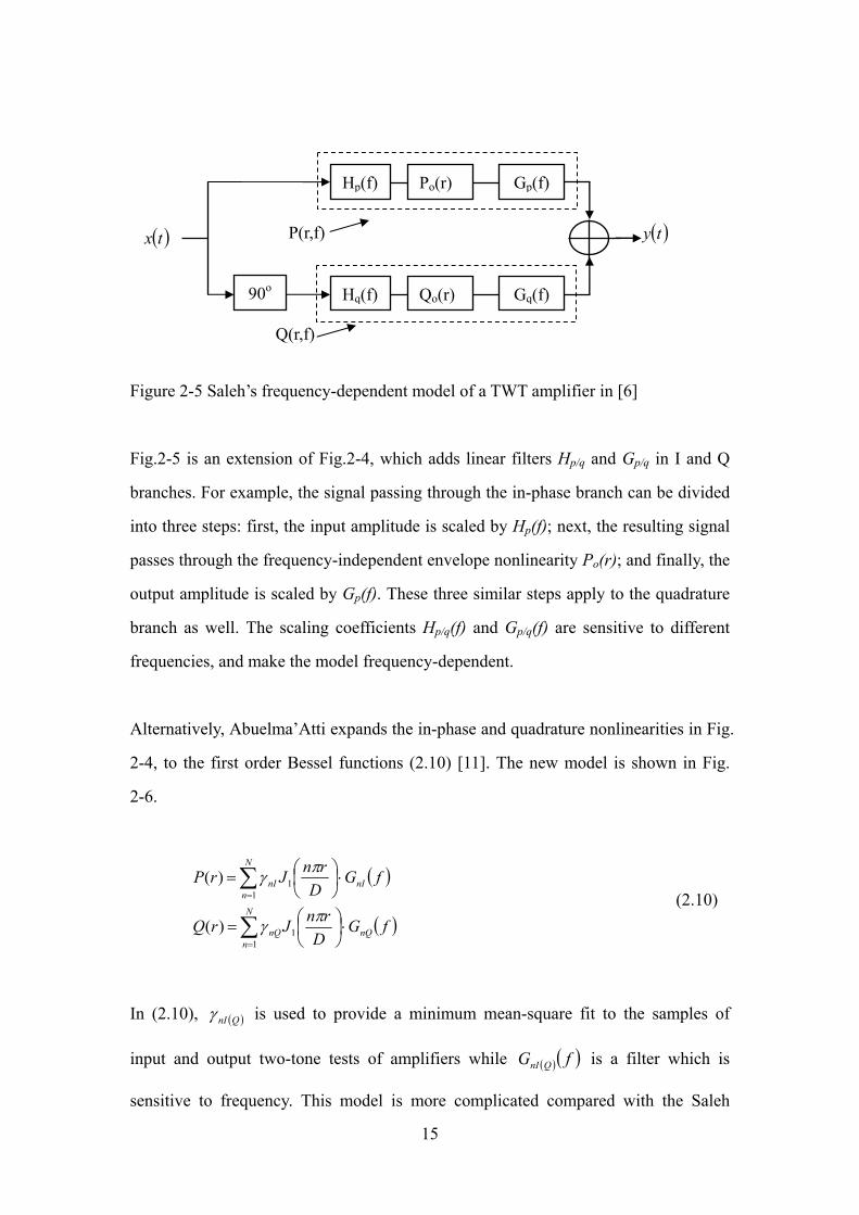
Figure 2-5 Saleh’s frequency-dependent model of a TWT amplifier in [6]
Fig.2-5 is an extension of Fig.2-4, which adds linear filters Hp/q and Gp/q in I and Q
branches. For example, the signal passing through the in-phase branch can be divided
into three steps: first, the input amplitude is scaled by Hp(f); next, the resulting signal
passes through the frequency-independent envelope nonlinearity Po(r); and finally, the
output amplitude is scaled by Gp(f). These three similar steps apply to the quadrature
branch as well. The scaling coefficients Hp/q(f) and Gp/q(f) are sensitive to different
frequencies, and make the model frequency-dependent.
Alternatively, Abuelma’Atti expands the in-phase and quadrature nonlinearities in Fig.
2-4, to the first order Bessel functions (2.10) [11]. The new model is shown in Fig.
2-6.
( )
( )fGD
rnJrQ
fGD
rnJrP
nQ
N
nnQ
nI
N
nnI
⋅⎟⎠⎞
⎜⎝⎛=
⋅⎟⎠⎞
⎜⎝⎛=
∑
∑
=
=
11
11
)(
)(
πγ
πγ (2.10)
In (2.10), ( )QnIγ is used to provide a minimum mean-square fit to the samples of
input and output two-tone tests of amplifiers while ( ) ( )fG QnI is a filter which is
sensitive to frequency. This model is more complicated compared with the Saleh
15
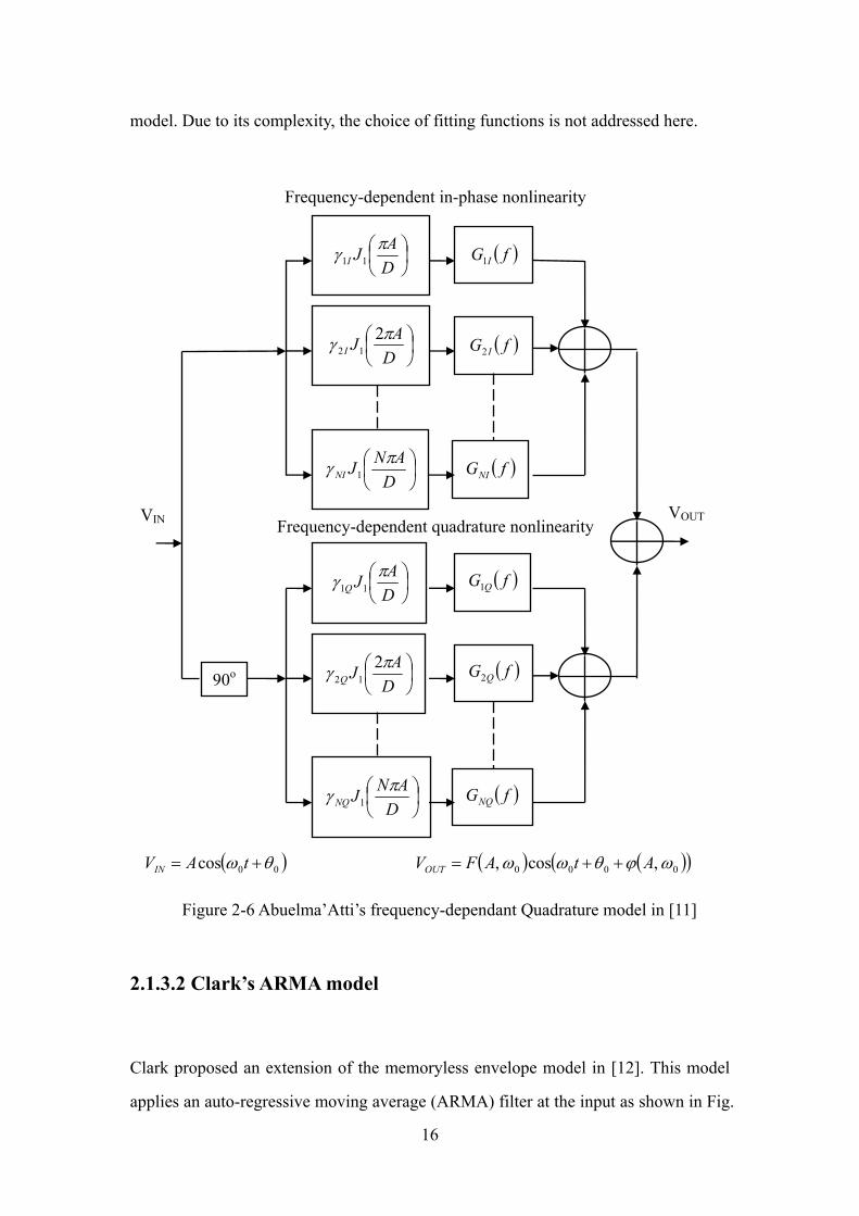
model. Due to its complexity, the choice of fitting functions is not addressed here.
⎟⎠⎞
⎜⎝⎛
DAJIπγ 11
⎟⎠⎞
⎜⎝⎛
DAJIπγ 2
12
⎟⎠⎞
⎜⎝⎛
DANJNIπγ 1
( )fG I1
( )fG I2
( )fGNI
Figure 2-6 Abuelma’Atti’s frequency-dependant Quadrature model in [11]
2.1.3.2 Clark’s ARMA model
emoryless envelope model in [12]. This model Clark proposed an extension of the m
applies an auto-regressive moving average (ARMA) filter at the input as shown in Fig.
⎟⎠⎞
⎜⎝⎛
DAJQπγ 11
⎟⎠⎞
⎜⎝⎛
DAJQπγ 2
12
⎟⎠⎞
⎜⎝⎛
DANJNQπγ 1
( )fG Q1
( )fGNQ
( )fG Q2 90 o
Frequency-dependent in-phase nonlinearity
Frequency-dependent quadrature nonlinearity VOUT VIN
( )00cos θω += tAVIN ( ) ( )( )0000 ,cos,ω ω ωϕθ AtAFVOUT ++=
16
2-7.
Propagation Input Delay
b(N) b(1) b(0)
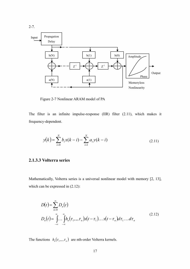
Figure 2-7 Nonlinear ARAM model of PA
he filter is an infinite impulse-response (IIR) filter (2.11), which makes it
(2.11)
.1.3.3 Volterra series
athematically, Volterra series is a universal nonlinear model with memory [2, 13],
(2.12)
The functions
T
frequency-dependent.
( ) ∑∑==
−−−=N
ii
N
ii ikyaikxbky
10)()(
2
M
which can be expressed in (2.12):
( ) ( )
( ) ( ) ( ) ( )∫∫
∑∞
∞−
∞
∞−
∞
=
−−=
=
nnnnn
nn
ddtxtxhtD
tDtD
ττττττ KKK 111
0
,,,
( )nnh ττ ,,,1 are nth-order Volterra kernels.
Z-1
a(N) a(1)
Z-1
Amplitude
Phase
Output
Memoryless Nonlinearity
17

Practically, there is a serious drawback of the Volterra model, in that it needs a large
aper [18] proposed a Wiener system. It consists of several subsystems connected in
ach subsystem has a linear time invariant (LTI) system with function of H(),
uppose the envelope frequency is ωm, and the input signal is z, the functions of F()
number of coefficients to represent Volterra kernels. Therefore, it is derived into two
special cases: memory polynomial model [13-17] and Wiener model [16].
P
parallel, as shown in Fig. 2-8.
Figure 2-8 Parallel Wiener model in [18]
E
followed by frequency-dependent complex power series with function of F().
S
is:
( ) ( ) ( ) ( ) 1212
331 ..., −
−+++= nmnmmm zazazazF ωωωω (2.13)
here a(ωm) are the coefficients of the frequency-dependent complex polynomial.
he LTI system H() has the following characteristic function:
w
T
( )ty
( )tr
( )tyP~
( )ty2~
( )ty1~
( )tzP
( )tz1 ( )ω1H ( )ω,1 zF
( )ω,2 zF ( )ω2H
( )tz2
( )ωPH ( )ω,zFP
18
( ) ( ) ( )mijmimi eHH ωωω Ω= (2.14)
hen an input signal Acos(ωmt) is applied, the output is:
W
( ) ( )
( )
( ) ( ) ( )
( ) ( ) ( )( )( )( ) ( ) ( )( )( )
( ) ( ) ( )( )( )
( ) ( ) ( )( )( )∑∑
∑
∑
∑
∑
= =
−−
= −−
=
−−
=
=
Ω+=
⎪⎪⎭
⎪⎪⎬
⎫
⎪⎪⎩
⎪⎪⎨
⎧
Ω++
+Ω++
Ω+
=
+++=
=
=
p
i
n
k
kmimmimik
p
i nmimmimian
mimmimi
mimmimi
p
i
nminmimi
p
iii
p
iip
tHAa
tHAa
tHAa
tHAa
zazaza
zF
tyty
1 1
12,12
1 12,2
3,3
,1
1
12,12
3,3,1
1
1
cos
cos...
cos
cos
...
~
ωωωω
ωωωω
ωωωω
ωωωω
ωωω (2.15)
here p is the number of parallel branches and n is the order of polynomial.
he parameters of H() can be acquired using cross-correlation function of the input.
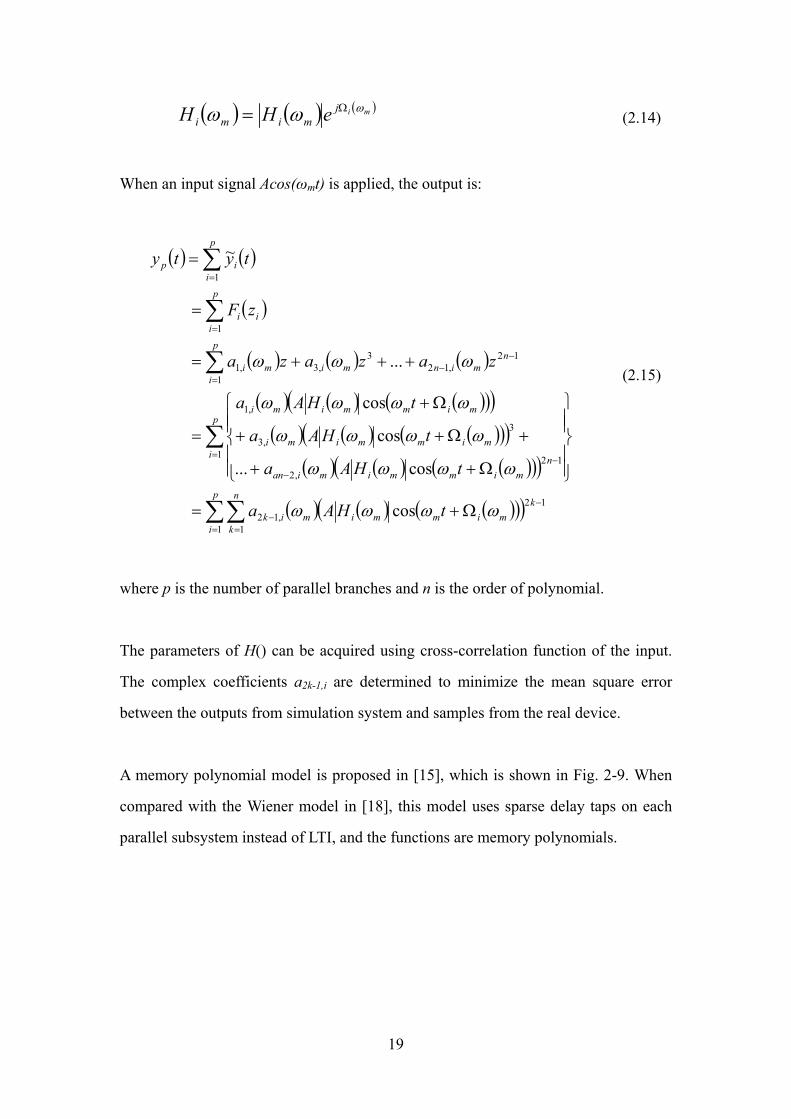
memory polynomial model is proposed in [15], which is shown in Fig. 2-9. When
w
T
The complex coefficients a2k-1,i are determined to minimize the mean square error
between the outputs from simulation system and samples from the real device.
A
compared with the Wiener model in [18], this model uses sparse delay taps on each
parallel subsystem instead of LTI, and the functions are memory polynomials.
19
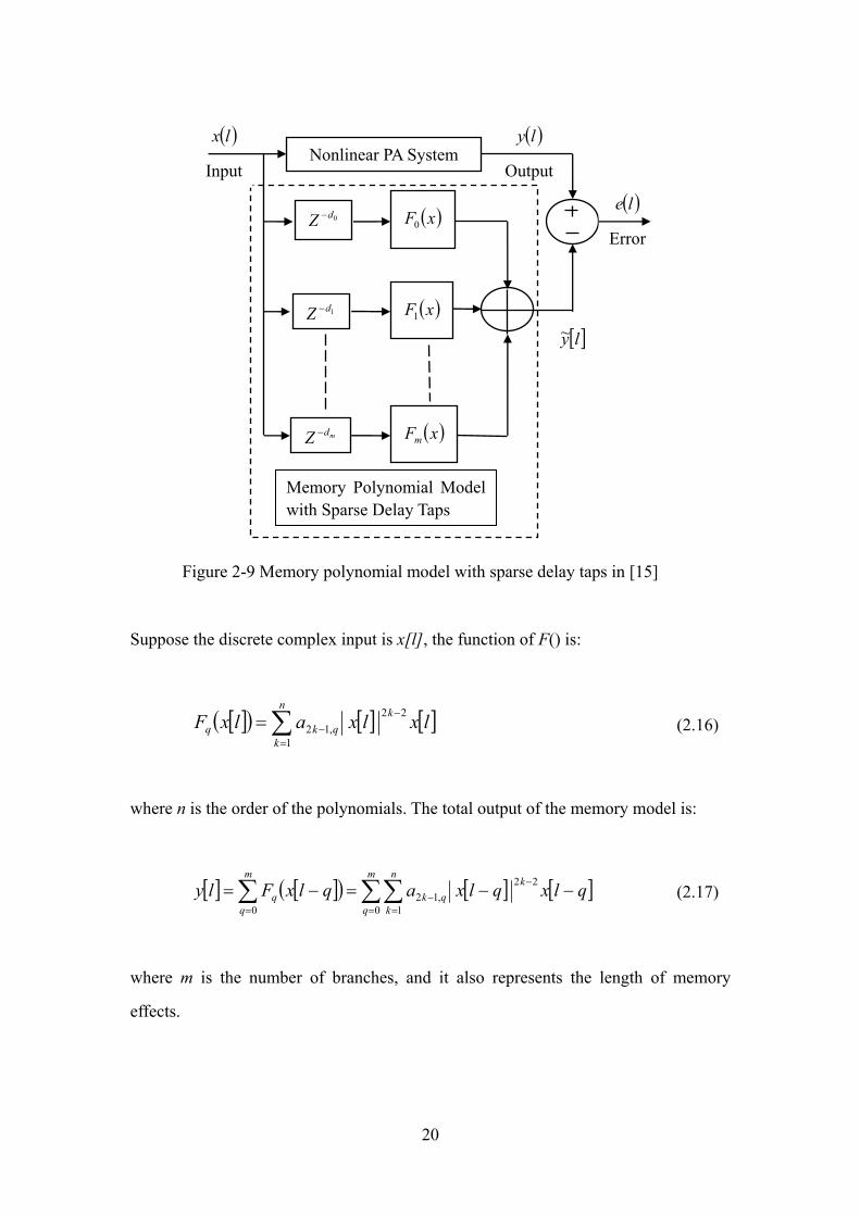
Figure 2-9 Memory polynomial model with sparse delay taps in [15]
Suppose the discrete complex input is x[l], the function of F() is:
[ ]( ) [ ] [ ]∑=
−−=
n
k
kqkq lxlxalxF
1
22,12 (2.16)
where n is the order of the polynomials. The total output of the memory model is:
[ ] [ ]( ) [ ] [∑∑∑= =
−−
=
−−=−=m
q
n
k
kqk
m
qq qlxqlxaqlxFly
0 1
22,12
0
] (2.17)
where m is the number of branches, and it also represents the length of memory
effects.
( )ly
Output
( )lx
( )le
Error
Input
( )xF0 0dZ −
[ ]ly~
( )xF1
mdZ −
( )xFm
1dZ −
Nonlinear PA System
Memory Polynomial Model with Sparse Delay Taps
20
2.1.3.4 Neural network based model
In [19], Ahemed et al. propose a new artificial neural network (ANN) model for
power amplifiers. It is shown in Fig. 2-10. The inputs for this model are current input
signal and optimum (sparse) delayed input signal. The ANN uses back propagation
(BP) (described in 2.2.4.1) for modifying the weights to approximate the
nonlinearities and memory effects of real amplifiers.
Figure 2-10 Time-delay neural network for PA model in [19]
2.2 Predistortion for power amplifiers
Efficiency is a primary concern for the PA designers. However, the trade off for high
efficiency is normally a decrease in linearity, and the decreasing linearity contributes
to spectral interference outside the intended bandwidth. Fortunately, there are
linearization techniques that allow PAs to be operated at high power efficiency while
with satisfying linearity requirements. There are many linearization techniques, such
as predistortion [16], feedback [1, 2] and feed-forward[2]. Among them, predistortion
promises better efficiency and lower cost. Because an ideal predistorter (PD) would
21
be an inverse function of the PA model, there are various PD models relative to the
different PA models.
2.2.1 AM/AM and AM/PM conversion
The simplest concept for the predistorter is to generate the inverse of the AM/AM and
AM/PM functions.
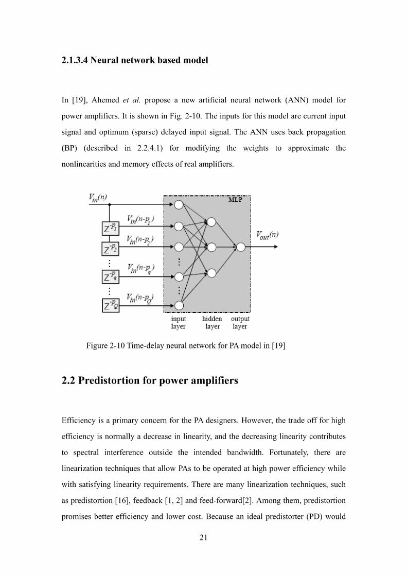
In 1983, J. Namiki proposed a nonlinear compensation technique (predistorter and
prerotation) and its controller in [20]. The predistorter uses a cubic law device and
phase shifter to compensate AM/AM and AM/PM distortion in PA. Experiment in [20]
shows that the spectral regrowth has been reduced by 10dB. This kind of predistortion
has been improved thereafter.
Figure 2-11 Predistorter proposed in [20]
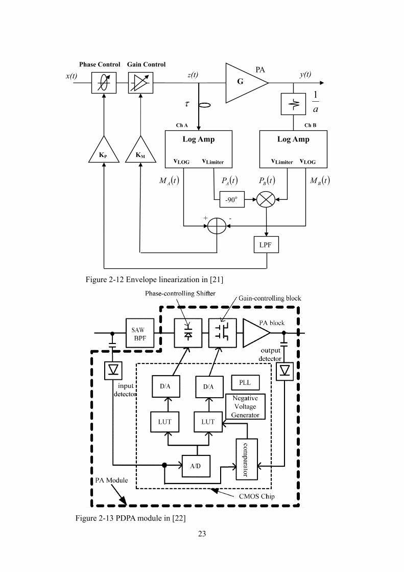
As shown in Fig. 2-12, log amps and phase detectors are used at the input and output
of the PA to estimate the instantaneous complex PA gain. This information is fed back
to a voltage controlled variable attenuator and phase shifter, which is for AM/AM and
AM/PM conversion [21]. Simulation of this predistortion has showed a 10 dB
improvement on ACPR.
22
x(t)
Phase Control Gain Control
( )tM A ( )tP A ( )tPB M ( )tB
Ch A Ch B
+ -
a1
τ
PA
G
z(t)
y(t)
Log Amp
vLOG vLimiter
Log Amp
vLimiter vLOG
-90o
LPF
KP KM
Figure 2-12 Envelope linearization in [21]
Figure 2-13 PDPA module in [22]
23
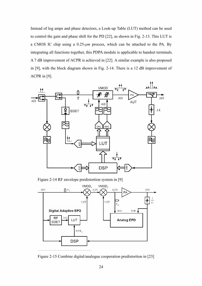
Instead of log amps and phase detectors, a Look-up Table (LUT) method can be used
to control the gain and phase shift for the PD [22], as shown in Fig. 2-13. This LUT is
a CMOS IC chip using a 0.25-μm process, which can be attached to the PA. By
integrating all functions together, this PDPA module is applicable to handset terminals.
A 7 dB improvement of ACPR is achieved in [22]. A similar example is also proposed
in [9], with the block diagram shown in Fig. 2-14. There is a 12 dB improvement of
ACPR in [9].
Figure 2-14 RF envelope predistortion system in [9]
Figure 2-15 Combine digital/analogue cooperation predistortion in [23]
24
An upgraded predistorter which combines Fig. 2-12 and Fig. 2-14 is shown in Fig.
2-15 [23]. In this two-stage structure, the analogue envelope predistorter is used as an
inner loop to correct slowly varying changes in gain, effectively compensating for
long time constant memory effects, while the digital envelope predistorter forms the
outer loop that corrects the distortion over a wide bandwidth. A 16 dB improvements
on ACPR is achieved in [23].
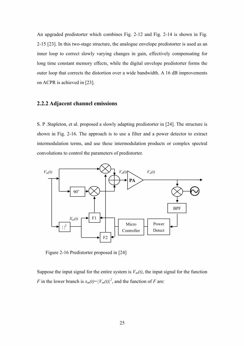
2.2.2 Adjacent channel emissions
S. P .Stapleton, et al. proposed a slowly adapting predistorter in [24]. The structure is
shown in Fig. 2-16. The approach is to use a filter and a power detector to extract
intermodulation terms, and use these intermodulation products or complex spectral
convolutions to control the parameters of predistorter.
Xm(t)
Vm(t) Vd(t) Va(t)
90o
PA
F1
F2
| |2 Micro
Controller Power Detect
BPF
Figure 2-16 Predistorter proposed in [24]
Suppose the input signal for the entire system is Vm(t), the input signal for the function
F in the lower branch is xm(t)=|Vm(t)|2, and the function of F are:
25
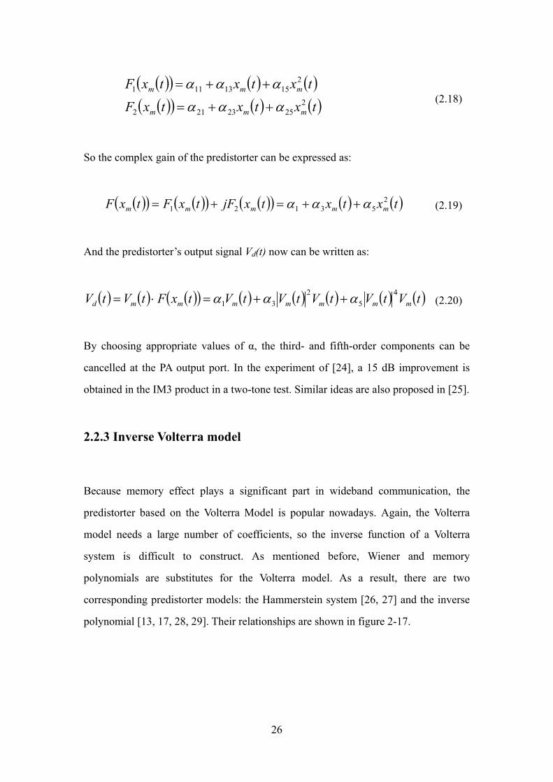
( )( ) ( ) ( )( )( ) ( ) ( )txtxtxF
txtxtxF
mmm
mmm2
2523212
21513111
ααα
ααα
++=
++= (2.18)
So the complex gain of the predistorter can be expressed as:
( )( ) ( )( ) ( )( ) ( ) ( )txtxtxjFtxFtxF mmmmm2
53121 ααα ++=+= (2.19)
And the predistorter’s output signal Vd(t) now can be written as:
( ) ( ) ( )( ) ( ) ( ) ( ) ( ) ( )tVtVtVtVtVtxFtVtV mmmmmmmd4
52
31 ααα ++=⋅= (2.20)
By choosing appropriate values of α, the third- and fifth-order components can be
cancelled at the PA output port. In the experiment of [24], a 15 dB improvement is
obtained in the IM3 product in a two-tone test. Similar ideas are also proposed in [25].
2.2.3 Inverse Volterra model
Because memory effect plays a significant part in wideband communication, the
predistorter based on the Volterra Model is popular nowadays. Again, the Volterra
model needs a large number of coefficients, so the inverse function of a Volterra
system is difficult to construct. As mentioned before, Wiener and memory
polynomials are substitutes for the Volterra model. As a result, there are two
corresponding predistorter models: the Hammerstein system [26, 27] and the inverse
polynomial [13, 17, 28, 29]. Their relationships are shown in figure 2-17.
26

Memory Polynomial Inverse Memory Polynomial Polynomial Volterra Model Wiener Model Hammerstein System Mathematical Model PA Model PD Model
Figure 2-17 Relation between Volterra model and its PA/PD model
2.2.3.1 Inverse memory polynomial model
The Volterra series in (2.12) can be expressed in discrete time as:
( ) ( ) ( ) ( )
( ) ( ) ( )∑∑∑
∑∑∑
= = =
= ==
+−−−+
−−+−=
N
k
N
l
N
mmlk
N
k
N
llk
N
kk
mnxlnxknxh
lnxknxhknxhny
0 0 0
3,,
0 0
2,
0
1
... (2.21)
where N is the discrete system memory length, x(n) and y(n) are input and output.
Paper [13] applies the indirect learning architecture [30] to help to embed the Volterra
model into the PD, which is shown in Fig. 2-18.
Figure 2-18 Indirect learning architecture for the predistorter
27
The idea in this paper is to uses two identical Volterra models (2.21) for the
predistorter and training. The training process applies a recursive least squares
algorithm. After the training, the innovation α[n] approaches zero, the output y[n]
approaches the input x[n], which means the overall system become linear. Similar
polynomial models have been proposed, but with different ways to calculate the
coefficients, such as Newton method[28], genetic algorithms[29] and least-squares
solution[17].
2.2.3.2 Hammerstein model
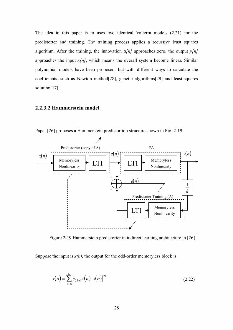
Paper [26] proposes a Hammerstein predistortion structure shown in Fig. 2-19.
( )ne + -
( )ny ( )nz ( )nx
PA
Predistorter Training (A)
Memoryless Nonlinearity LTI LTI
LTI
Memoryless Nonlinearity
Memoryless Nonlinearity
k1
Predistorter (copy of A)
Figure 2-19 Hammerstein predistorter in indirect learning architecture in [26]
Suppose the input is x(n), the output for the odd-order memoryless block is:
( ) ( ) ( )∑=
+=K
k
kk nxnxcnv
0
212 (2.22)
28
And the output z(n) from LTI system is:
( ) ( ) ( )∑∑==
−+−=Q
P
pp qnvbpnzanz
01 (2.23)
So the entire relationship between input x(n) and output z(n) is:
( ) ( ) ( ) ( )∑ ∑∑= =
+=
+−=Q
q
K
k
kkq
P
pp nxnxcbpnzanz
0 0
212
1 (2.24)
The coefficients can be optimized by using Narendra-Gallman algorithm [26], and the
simulation result has shown a 38 dB ACPR reduction.
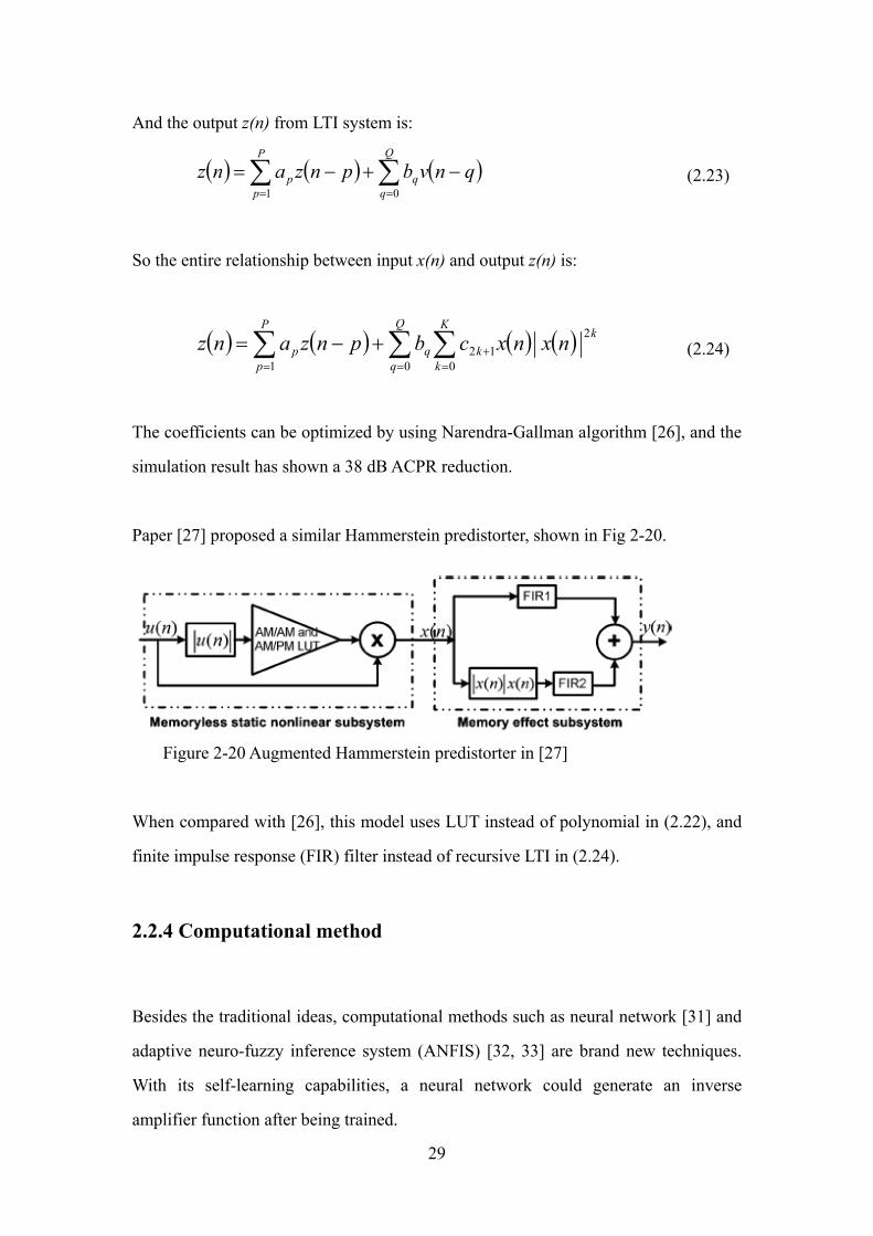
Paper [27] proposed a similar Hammerstein predistorter, shown in Fig 2-20.
Figure 2-20 Augmented Hammerstein predistorter in [27]
hen compared with [26], this model uses LUT instead of polynomial in (2.22), and
2.2.4 Computational method
Besides the traditional ideas, computational methods such as neural network [31] and
W
finite impulse response (FIR) filter instead of recursive LTI in (2.24).
adaptive neuro-fuzzy inference system (ANFIS) [32, 33] are brand new techniques.
With its self-learning capabilities, a neural network could generate an inverse
amplifier function after being trained.
29
2.2.4.1 Neural network
Neural networks are modeled after the physical architecture of human brains and they
can use simple processing elements to perform complex nonlinear behaviors.
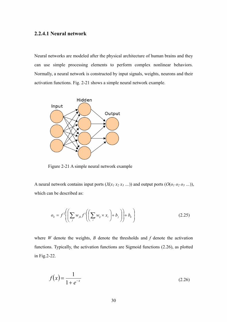
Normally, a neural network is constructed by input signals, weights, neurons and their
activation functions. Fig. 2-21 shows a simple neural network example.
Figure 2-21 A simple neural network example
neural network contains input ports (X(x1 x2 x3 …)) and output ports (O(o1 o2 o3 …)),
(2.25)
here W denote the weights, B denote the thresholds and f denote the activation
A
which can be described as:
⎟⎟⎠
⎞⎜⎜⎝
⎛+⎟
⎟⎠
⎞⎜⎜⎝
⎛⎟⎟⎠
⎞⎜⎜⎝
⎛+⎟
⎠
⎞⎜⎝
⎛×= ∑ ∑ k
jj
iiijjkk bbxwfwfo 12
w
functions. Typically, the activation functions are Sigmoid functions (2.26), as plotted
in Fig.2-22.
( ) xexf −+=
11
(2.26)
30

Figure 2-22 Sigmoid function
Back-propagation (BP) learning algorithm [34, 35] can be applied to adjust the
utput date sets are X(x1 x2 x3 …) and Y(y1 y2
3 …), and the neural network are two-layer structure (2.25) with the Sigmoid
weights. Suppose the training input o
y
function (2.26), the adjustment for weights are:
( )( ) jkkkkjk oooyow
⎛
−−=Δ 1
( )( ) ( )jjk
jkkkkkij oowoyoow −⎟⎠
⎞⎜⎝
−−=Δ ∑ 11α
α
(2.27)
In (2.27), o means what we get from the layers of neural netwo
we want from the neural network, and α is the learning rate.
Two-valued or Boolean logic is a well-known theory. But it is impossible to solve all
ariables. Most real-world
roblems are characterized by a representation language to process incomplete,
rk, while y means what
2.2.4.2 Fuzzy system and Fuzzy inference system
problems by mapping all kinds of situation into two-valued v
p
imprecise, vague or uncertain information. Fuzzy logic gives the formal tools to
reason about such uncertain information. A fuzzy system is one which employs fuzzy
logic [36].
31

A form of if-then rule in fuzzy system is shown as below:
if x is A then y is B
here A and B are linguistic values defined by fuzzy sets on the ranges x and y,
respect the rule "x is A" is called the antecedent or premise, while
e then-part of the rule "y is B" is called the consequent or conclusion.
The step is:
Compare the input variables with the membership functions on the antecedent
shown as μA1, μA2,
μB1, μB2,. This step is called fuzzification.
ule.
rule depending on the weight, i.e.,
w1☓f1 and w2☓f2
Aggregate the qualified consequents to produce a final output (2.28). This step is
w
ively. The if-part of
th
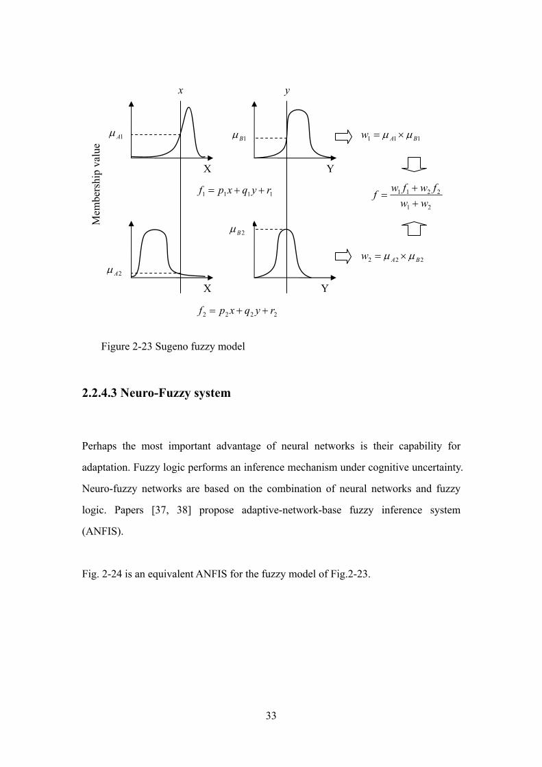
The Fuzzy Inference System (FIS) [37] is a system formed from the if-then rules. For
example, we have two-input (x, y), two-rules, and defined the rules as:
Rule 1 if x is A1 and y is B1, then f1=p1x+q1y+r1
Rule 2 if x is A2 and y is B2, then f2=p2x+q2y+r2
s of fuzzy reasoning performed by Sugeno-type FIS
part to obtain the membership values of each linguistic label,
Combine the membership values on the antecedent part to get weight of each r
For example: w1=μA1☓μB1
Generate the qualified consequent of each
called defuzzification.
21 ww +
All the steps are shown in fig. 2-23.
2211 fwf += (2.28) fw
32
33
2.2.4.3 Neuro-Fuzzy system
ural networks is their capability for
inference mechanism under cognitive uncertainty.
euro-fuzzy networks are based on the combination of neural networks and fuzzy
Figure 2-23 Sugeno fuzzy model
Perhaps the most important advantage of ne
adaptation. Fuzzy logic performs an
N
logic. Papers [37, 38] propose adaptive-network-base fuzzy inference system
(ANFIS).
Fig. 2-24 is an equivalent ANFIS for the fuzzy model of Fig.2-23.
1Bμ 1Aμ
X Y
X Y
Mem
bers
hip
valu
e x y
2Aμ
111 BAw μμ ×=
2Bμ
222 BAw μμ ×=
111 ryqxpf 1 ++=
21
2211
wwfwfwf
++
=
2222 ryqxpf + +=
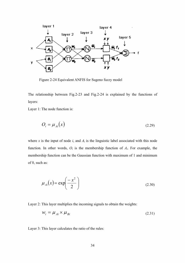
Figure 2-24 Equivalent ANFIS for Sugeno fuzzy model
The relationship between Fig.2-23 and Fig.2-24 is explained by the functions of
layers:
Layer 1: The node function is:
( )xO Aii μ= (2.29)
where x is the input of node i, and Ai is the linguistic label associated with this node
function. In other words, Oi is the membership function of Ai. For example, the
membership function can be the Gaussian function with maximum of 1 and minimum
of 0, such as:
( ) ⎟⎟⎠
⎞⎜⎜⎝
⎛ −=
2exp
2xxAiμ (2.30)
Layer 2: This layer multiplies the incoming signals to obtain the weights:
BiAiiw μμ ×= (2.31)
Layer 3: This layer calculates the ratio of the rules:
34
2,1,21
=+
= iww
ww ii (2.32)
Layer 4: This layer calculates the output for each consequent and multiplies its ratio in
(2.32):
( ) 2,1=++= iryqxpwfw iiiiii (2.33)
Layer 5: The single node in this layer gives the overall output as the summation of all
incoming signals:
∑ ++
==21
2211
wwfwfwfwf ii (2.34)
It will get the same result as (2.28).
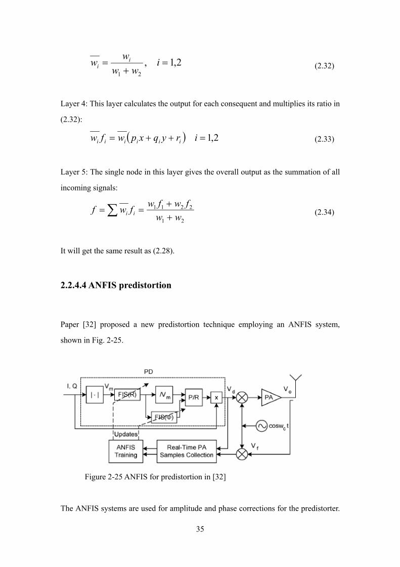
2.2.4.4 ANFIS predistortion
Paper [32] proposed a new predistortion technique employing an ANFIS system,
shown in Fig. 2-25.
Figure 2-25 ANFIS for predistortion in [32]
The ANFIS systems are used for amplitude and phase corrections for the predistorter.
35
The membership functions for this ANFIS are Gaussian functions. Experimental
results showed that with optimization, this ANFIS system can have a 26.3 dB
reduction on the third order IMD products in a two-tone test, or a 13 dB ACPR
reduction on wideband signals.
2.2.5 Injection predistortion
Injection is another simple type of predistortion. The idea is to add frequency
components at the input port of PA, which generate the same amplitudes but opposite
phases of the original intermodulation products at the output port, to counteract the
distortions.
2.2.5.1 Injection in two-tone test
The main target for injection in a two-tone test signal is to cancel the third-order
intermodulation products (IM3). There are different types of mechanisms to generate
IM3 at the output port of PAs.
Paper [39] uses the linear gain of the PA to remove the unwanted spectral lines, shown
in Fig. 2-26.
36
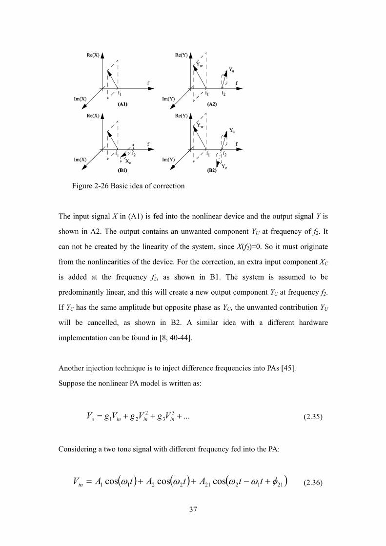
Figure 2-26 Basic idea of correction
The input signal X in (A1) is fed into the nonlinear device and the output signal Y is
shown in A2. The output contains an unwanted component YU at frequency of f2. It
can not be created by the linearity of the system, since X(f2)=0. So it must originate
from the nonlinearities of the device. For the correction, an extra input component XC
is added at the frequency f2, as shown in B1. The system is assumed to be
predominantly linear, and this will create a new output component YC at frequency f2.
If YC has the same amplitude but opposite phase as YU, the unwanted contribution YU
will be cancelled, as shown in B2. A similar idea with a different hardware
implementation can be found in [8, 40-44].
Another injection technique is to inject difference frequencies into PAs [45].
Suppose the nonlinear PA model is written as:
...33
221 +++= ininino VgVgVgV (2.35)
Considering a two tone signal with different frequency fed into the PA:
( ) ( ) ( )2112212211 coscoscos φωωωω +−++= ttAtAtAVin (2.36)
37
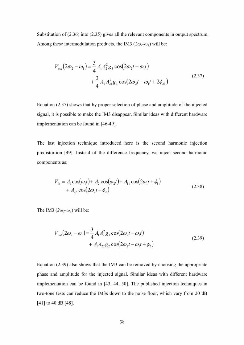
Substitution of (2.36) into (2.35) gives all the relevant components in output spectrum.
Among these intermodulation products, the IM3 (2ω2-ω1) will be:
( ) ( )
( )211232212
12322112
22cos43
2cos432
φωω
ωωωω
+−+
−=−
ttgAA
ttgAAVout
(2.37)
Equation (2.37) shows that by proper selection of phase and amplitude of the injected
signal, it is possible to make the IM3 disappear. Similar ideas with different hardware
implementation can be found in [46-49].
The last injection technique introduced here is the second harmonic injection
predistortion [49]. Instead of the difference frequency, we inject second harmonic
components as:
( ) ( ) ( )( )2222
11112211
2cos2coscoscos
φωφωωω
+++++=
tAtAtAtAVin
(2.38)
The IM3 (2ω2-ω1) will be:
( ) ( )
( )2122221
12322112
2cos
2cos432
φωω
ωωωω
+−+
−=−
ttgAA
ttgAAVout (2.39)
Equation (2.39) also shows that the IM3 can be removed by choosing the appropriate
phase and amplitude for the injected signal. Similar ideas with different hardware
implementation can be found in [43, 44, 50]. The published injection techniques in
two-tone tests can reduce the IM3s down to the noise floor, which vary from 20 dB
[41] to 40 dB [48].
38

2.2.5.2 Injection in wideband signals
Besides two-tone test, the injection technique has also been applied to wideband
communication signals. Paper [51] injects the third- and fifth-order distortion
components in the baseband block to eliminate the fundamental distortion. It assumes
that the amplifier nonlinearity can be expressed in a power series up to the fifth
degree:
55
44
33
221 iiiiio vgvgvgvgvgv ++++= (2.40)
And the input digital modulation which has magnitude c(t) and phase φ(t) and carrier
frequency ω:
( ) ( ) ( )( )( ) ( )( tQtIv
tttctv
s
i
ωω )φω
sincoscos
−=+=
(2.41)
where
( )( ) ( )( ) ss vtctQvtctI /)(sin/)(cos φφ ==
and vs is the average of |c(t)|. Therefore, average (I2+Q2)=1.
By substituting (2.41) into (2.40), the distorted output voltage appearing at the
fundamental frequency is:
( ) ( ) ( )( ) ( ) ( ) ( )( )
( ) ( ) ( )( )tQtIQIvg
tQtIQIvgtQtIvgtv
s
ssfunt
ωω
ωωωω
sincos85
sincos43sincos
22255
22331
−++
−++−= (2.42)
39

In (2.42), the second term is the third-order distortion, and the third term is the
fifth-order distortion. Now the cube of the desired signal is added into (2.41) as the
third-order distortion component:
( ) ( ) ( )( ) ( ){ }221sincos QIatQtIvtv si ++−= ωω (2.43)
Equation (2.42) will change to
( ) ( ) ( )( )( ) ( ) ( )( )
( ) ( ) ( )( )
( ) ( ) ( )( )
( ) ( ) ( )( )tQtIQIavg
tQtIQIavg
tQtIQIvg
tQtIQIavg
tQtIvgtv
s
s
s
s
sfunt
ωω
ωω
ωω
ωω
ωω
sincos94
sincos94
sincos43
sincos
sincos
322233
22233
2233
221
1
−++
−++
−++
−++
−=
(2.44)
In the calculation, the term that has a3 is ignored because it is too small. The third
term in (2.44) is the original third-order distortion. The second, fourth and fifth terms
are generated by the injected distortion component. In a weakly nonlinear region, the
input voltage vs is small, the fourth and fifth terms can be ignored, which makes (2.44)
become:
( ) ( ) ( )( )( ) ( ) ( )( )
( ) ( ) ( )( )tQtIQIvg
tQtIQIavg
tQtIvgtv
s
s
sfunt
ωω
ωω
ωω
sincos43
sincos
sincos
2233
221
1
−++
−++
−=
(2.45)
The second and third terms in (2.45) can cancel each other by choosing appropriate a:
40
2
1
3
43
svgga −= (2.46)
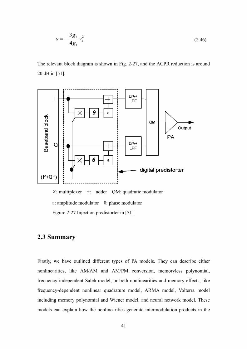
The relevant block diagram is shown in Fig. 2-27, and the ACPR reduction is around
20 dB in [51].
☓: multiplexer +: adder QM: quadratic modulator
a: amplitude modulator θ: phase modulator
Figure 2-27 Injection predistorter in [51]
2.3 Summary
Firstly, we have outlined different types of PA models. They can describe either
nonlinearities, like AM/AM and AM/PM conversion, memoryless polynomial,
frequency-independent Saleh model, or both nonlinearities and memory effects, like
frequency-dependent nonlinear quadrature model, ARMA model, Volterra model
including memory polynomial and Wiener model, and neural network model. These
models can explain how the nonlinearities generate intermodulation products in the
41

output spectrum, and how the memory effects cause asymmetries between the upper
and lower side band of these intermodulation products.
Secondly, according to these PA models, their inverse models are also depicted in this
chapter, such as AM/AM and AM/PM conversion, inverse Volterra model including
inverse memory polynomial and Hammerstein model, and the neural network model.
Besides these inverse PA models, the alternative technique, named injection, is also
presented here. This technique addresses the amplitude and phase of the unwanted
frequencies, and generates the same but with anti-phase phasors to counteract with the
originals. Such kind of technique can reduce the IM3 in two-tone tests.
However, the published predistortion techniques have different drawbacks. The
inverse memoryless PA predistortion can not deal with memory effects, which limits
its operation in wideband signal cases. The Volterra and its derivated models can
handle both nonlinearities and memory effects, but it is complicated to understand and
extract its coefficients. The neural network types have the similar problem that, we
can not explain what the coefficients mean. The injection can reduce IM3 products in
two-tone tests, but its reduction on spectral regrowth in wideband signals is not
completely down to the noise floor, as shown in the published papers.
New predistortion techniques which can deal with both nonlinearities and memory
effects, and easy to understand and implement is needed. In my research work, I
chose the injection as the fundamental predistortion technique. Improvements to the
published injection techniques are given in Chapter 3, 4 and 5. We focus its
application in the two-tone test in Chapter 3. It will reveal what the new problems
injection causes and how to solve them. Experimental results in different signal
conditions will be shown in the end of Chapter 3. In Chapter 4, such kind of injection
technique will be upgraded in order to work in wideband signals. In Chapter 5, after
analyzing LUT and injection working in wideband signal, a new predistortion
technique, which combines both LUT and injection, is proposed. It inherits the
42

advantages from both LUT and injection. We have also used a cascaded PA system
which has both significant nonlinearities and memory effects, to demonstrate its
abilities.
43

CHAPTER 3
IMPROVEMENTS OF INJECTION TECHNIQUES IN TWO-TONE TESTS
Firstly, we will introduce a general two-tone test and demonstrate both nonlinearities
and memory effects in a PA through a two-tone test. Secondly, we will discuss the
published techniques for measuring and reducing third-order intermodulation (IM3)
products in a two-tone test. Finally, we propose our improvements of these
techniques.
3.1 Introductions of two-tone tests
The two-tone test is a universally recognized technique in assessing amplifier
nonlinearities and memory effects [52]. Firstly, it is simple and easy to generate.
Secondly, it can vary the envelope throughout a wide dynamic range to test the
amplifier’s transfer characteristic. Thirdly, it is possible to vary the tone spacing,
which is the envelope base band frequency, to examine the amplifier’s memory
effects[9]. All these advantages mean it is considered to be the most severe test of
power amplifiers.
The normal format of a two-tone test is:
( ) ( )
mc
mc
in tAtAV
ωωωωωω
ωω
+=−=
+=
2
1
21 coscos
(3.1)
44
In (3.1), A is the amplitude for a single carrier, ω1 and ω2 are the two carriers’
frequencies, ωc is the centre frequency of the signal while ωm is half of the
tone-spacing. Using the trigonometric identity, (3.1) can also be written as:
( ) ( )ttAV mcin ωω coscos2= (3.2)
Equation (3.2) shows us that the two-tone test signal can also be treated as a sine
wave with frequency of ωc, modulated by an envelope which is another sine wave
with frequency of ωm. The overall maximum amplitude is 2A. Normally in RF
research, ωc>>ωm, ωc is in the RF frequency range of the PA, and ωm is in the
baseband frequency range that will causes memory effects. The reason is as follows.
The impedance seen by the input of the transistor varies with frequency in the
baseband range, because the bias decoupling circuit is required to behave low
impedance at low frequency but high impedance at carrier frequency. There are
baseband currents flowing in the bias circuit due to the second and higher order
nonlinearities of the transistor. These currents will result voltages that are
frequency-dependant [53]. Therefore, while the two-tone test is applied to a PA, the
difference frequency ωm voltage on the gate terminal modulates the gain and
generates nonlinearity products whose levels are dependent on this difference
frequency. In other words, these nonlinearities products will vary as the difference
frequency varies, which are memory effects. All the information of A, ωc , ωm in a
two-tone waveform is shown in Fig. 3-1.
45

Figure 3-1 A two-tone test signal
When this two-tone signal is applied to a PA, the signal will be amplified, with some
new intermodulation products created by the PA nonlinearities. This can be simply
explained by memoryless polynomial model. Suppose the characteristic of the PA is:
( ) ...55
44
33
221 +++++= xaxaxaxaxaxy (3.3)
We substitute (3.1) into (3.3), we will get the output:
( ) ( ) ( )[ ] ( ) ( )[ ]( ) ( )[ ] ( ) ( )[ ]( ) ( )[ ] ...coscos
coscoscoscos
coscoscoscos
521
55
421
44
321
33
221
22211
+++
++++
+++=
ttAa
ttAattAa
ttAattAaVy in
ωω
ωωωω
ωωωω
(3.4)
46

Take the third order intermodulation products (IM3) for example, (3.4) will yield:
( ) ( ) ( )( )( ) (( )( )( ) (( )
))
33122212122212
332313
2112212212
2112212212
2231133
43
41
2cos2cos2cos2cos
3cos3cos
AaCCCC
AaCC
tCtCtCtC
tCtCVy inIM
====
==
++++−+−+
+=
++−−
++
−−
ωωωωωωωω
ωω
ωωωω
ωωωω
ωω
ωωωωωωωω
ωω
(3.5)
In (3.5), we can see that there are six IM3 products. Among them, only C2ω1-ω2 and
C2ω2-ω1 will affect the in band spectrum since others are at frequencies far above ω1 or
ω2. And these two IM3 products mainly cause spectral interference in real-world
communication signals, which are the objects of linearization techniques.
3.2 Published measurements and injections for IM3
products in two-tone tests
Equation (3.5) is a simple case of using memoryless PAs. However, once the PA
shows a significant degree of memory effects, the coefficient a3 would change to be a
frequency-dependent parameter, so that the more complicated models listed in Section
2.1.3 are required. Thus, memory effects shown in IM3 in two-tone tests [52, 54, 55]
is an interesting and important topic for linearization techniques. Recent research
mainly focuses on the measurement and elimination of IM3 products. One of the
common ways to measure the IM3 in two-tone tests, is to vary the input power and
the tone spacing [15, 18]. Injection is a procedure that can be based on measurement
results, to remove these IM3 products, since the basic idea for injection is to generate
IM3 products at the output port, which have identical amplitudes but opposite phases
to the original ones.
47
3.2.1 Measurements on IM3 products
Since the power of IM3 products can be directly observed from spectrum analyzers,
the only problem is measurement of IM3 phases. IM3 phases are varying with time,
so we can not identify them with any particular values. One of the common ways to
evaluate IM3 phases is to define or create a reference sine wave with the same
frequency, and measure the phase difference.
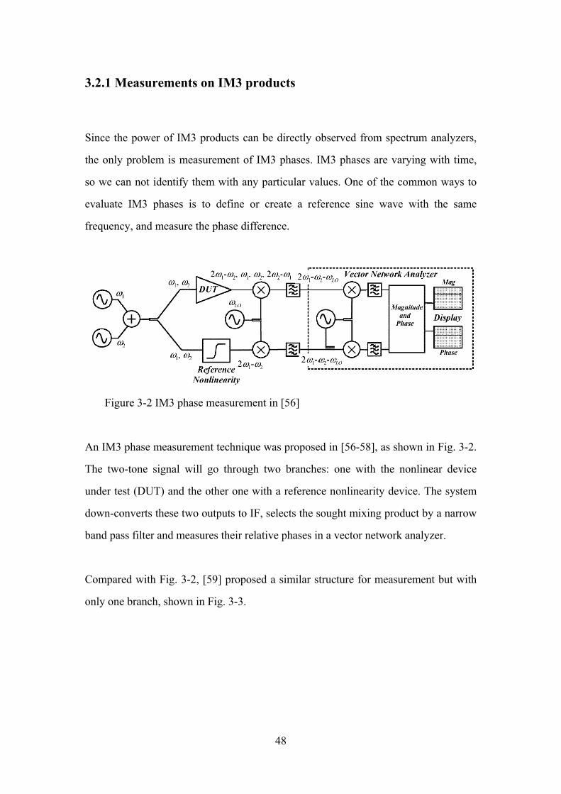
Figure 3-2 IM3 phase measurement in [56]
An IM3 phase measurement technique was proposed in [56-58], as shown in Fig. 3-2.
The two-tone signal will go through two branches: one with the nonlinear device
under test (DUT) and the other one with a reference nonlinearity device. The system
down-converts these two outputs to IF, selects the sought mixing product by a narrow
band pass filter and measures their relative phases in a vector network analyzer.
Compared with Fig. 3-2, [59] proposed a similar structure for measurement but with
only one branch, shown in Fig. 3-3.
48
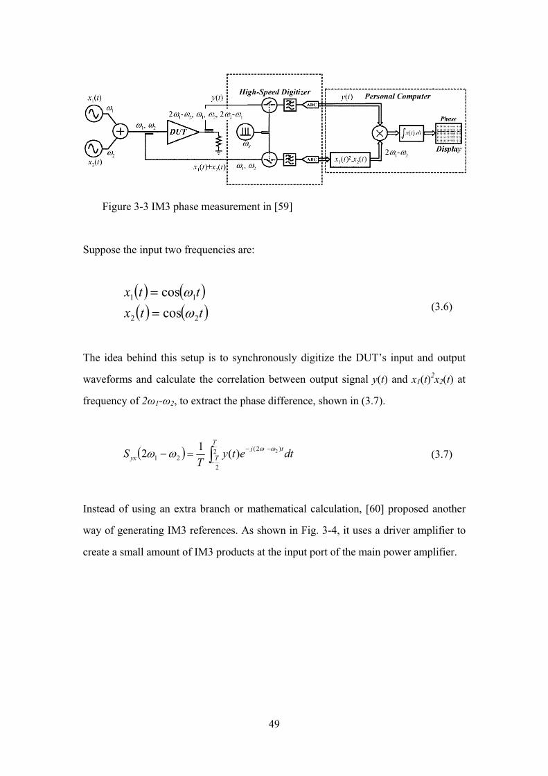
Figure 3-3 IM3 phase measurement in [59]
Suppose the input two frequencies are:
( ) ( )( ) ( )ttx
ttx
22
11
coscos
ωω
==
(3.6)
The idea behind this setup is to synchronously digitize the DUT’s input and output
waveforms and calculate the correlation between output signal y(t) and x1(t)2x2(t) at
frequency of 2ω1-ω2, to extract the phase difference, shown in (3.7).
( ) ∫−−−=− 2
2
)2(21
2)(12T
Ttj
yx dtetyT
S ωωωω (3.7)
Instead of using an extra branch or mathematical calculation, [60] proposed another
way of generating IM3 references. As shown in Fig. 3-4, it uses a driver amplifier to
create a small amount of IM3 products at the input port of the main power amplifier.
49
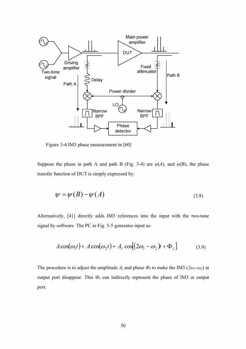
Figure 3-4 IM3 phase measurement in [60]
Suppose the phase in path A and path B (Fig. 3-4) are ψ(A), and ψ(B), the phase
transfer function of DUT is simply expressed by:
)()( AB ψψψ −= (3.8)
Alternatively, [41] directly adds IM3 references into the input with the two-tone
signal by software. The PC in Fig. 3-5 generates input as:
( ) ( ) ( )[ ]II tAtAtA Φ+−++ 2121 2coscoscos ωωωω (3.9)
The procedure is to adjust the amplitude AI and phase ФI to make the IM3 (2ω1-ω2) at
output port disappear. This ФI can indirectly represent the phase of IM3 at output
port.
50
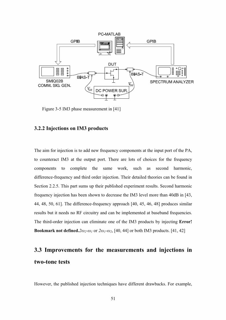
Figure 3-5 IM3 phase measurement in [41]
3.2.2 Injections on IM3 products
The aim for injection is to add new frequency components at the input port of the PA,
to counteract IM3 at the output port. There are lots of choices for the frequency
components to complete the same work, such as second harmonic,
difference-frequency and third order injection. Their detailed theories can be found in
Section 2.2.5. This part sums up their published experiment results. Second harmonic
frequency injection has been shown to decrease the IM3 level more than 40dB in [43,
44, 48, 50, 61]. The difference-frequency approach [40, 45, 46, 48] produces similar
results but it needs no RF circuitry and can be implemented at baseband frequencies.
The third-order injection can eliminate one of the IM3 products by injecting Error!
Bookmark not defined.2ω2-ω1 or 2ω1-ω2, [40, 44] or both IM3 products. [41, 42]
3.3 Improvements for the measurements and injections in
two-tone tests
However, the published injection techniques have different drawbacks. For example,
51

in [42], good results were achieved but with the PA working somewhat below the
compression point. The injection technique described in [39] needs a large number of
measurements. There are three novel improvements to third-order injection techniques
in our work.
1) A new way of generating a reference against which to measure IM3 products.
A completed two-tone IM3 characterization requires magnitude and phase
measurements [52, 54, 62]. Finding an IM3 reference is a general and useful
approach. We propose a virtual calculated IM3 reference which only comes from the
output two main tones. The technique produces accurate measurement results without
the extra hardware [56-58] or complicated mathematical functions [52, 55, 59].
2) A new mathematical description of the relationship between injected and output
IM3 products, including their amplitude and phase.
The injection technique requires the generation of anti-phase phasors to cancel the
IM3 products at the output port. In some published works, manual tuning is used to
adjust these phases. We propose a mathematical description of the relationship
between injected and output IM3 products, from which these anti-phase phasors can
be precisely calculated. A similar description proposed in [39], was based on the
measurement of power, while our work is based on the measurement of amplitude and
phase. As a result, the earlier method can not reveal the interactions between upper
and lower side band injected IM3 products, and hence needs large measurement times.
This will be explained in Section 3.3.3.
3) A new view of the interaction between the lower and upper IM3 products, which
affects the dual sideband injection.
Third-order injection uses input lower third-order intermodulation products (IM3L) to
52
eliminate output IM3L and input upper third-order intermodulation products (IM3U)
to eliminate output IM3U, separately. However, when these two injected products are
introduced together, they will affect each other at the output port because of the PA’s
nonlinearities. The frequency relationships can be written as: 2ω1-ω2=ω1+ω2-(2ω2-ω1)
and 2ω2-ω1=ω1+ω2-(2ω1-ω2). We define these to be interactions in our work. The
significance of the interaction depends on the third-order nonlinearity of the PA.
When the PA is working well below compression point, dual sideband predistortion
can be achieved perfectly without considering the interaction. For example, [42]
shows a perfect IM3 elimination without detecting interactions. In that work, the IM3s
are -30dBc relative to the two-tone carriers before predistortion, suggesting that the
PA is not driven hard, and the IM3s are only 20dB above the noise floor which limits
the observation range. If the PA is driven harder and the spectrum analyzer is working
with higher sensitivity to have a wider observation range, the effects of interactions
will become more apparent. In our work, the PA is operated beyond the 1dB
compression point, thus a completed matrix for both IM3 products suppression is
proposed in Section 3.3.3.
3.3.1 IM3 reference
Injection can achieve perfect distortion correction or it can make the result worse,
depending on whether the correct phase in used. Hence measuring the phases of
output IM3s plays an important role in injection. One solution is to generate an IM3
reference and define the IM3 phase as the difference between the reference and the
IM3 product. We will describe the experimental setup and introduce a new method of
generating the IM3 reference.
53
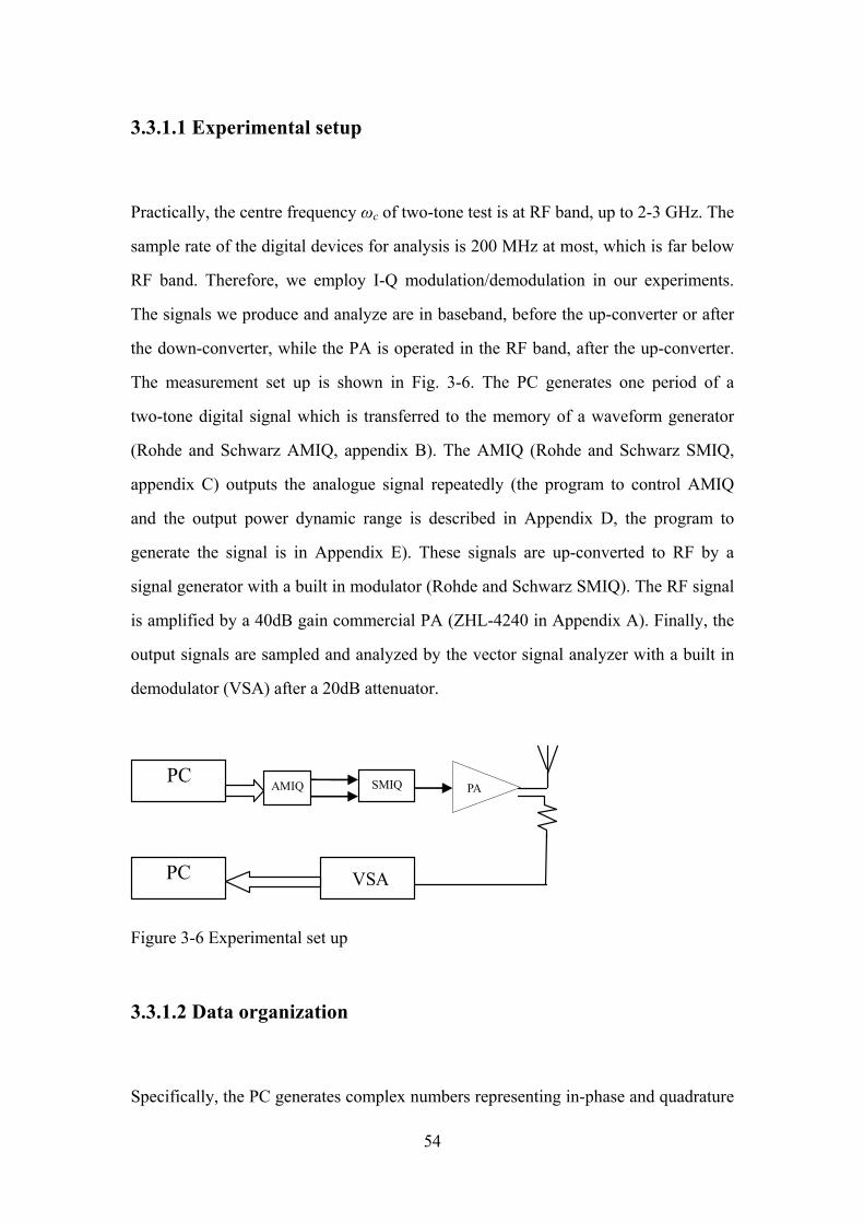
3.3.1.1 Experimental setup
Practically, the centre frequency ωc of two-tone test is at RF band, up to 2-3 GHz. The
sample rate of the digital devices for analysis is 200 MHz at most, which is far below
RF band. Therefore, we employ I-Q modulation/demodulation in our experiments.
The signals we produce and analyze are in baseband, before the up-converter or after
the down-converter, while the PA is operated in the RF band, after the up-converter.
The measurement set up is shown in Fig. 3-6. The PC generates one period of a
two-tone digital signal which is transferred to the memory of a waveform generator
(Rohde and Schwarz AMIQ, appendix B). The AMIQ (Rohde and Schwarz SMIQ,
appendix C) outputs the analogue signal repeatedly (the program to control AMIQ
and the output power dynamic range is described in Appendix D, the program to
generate the signal is in Appendix E). These signals are up-converted to RF by a
signal generator with a built in modulator (Rohde and Schwarz SMIQ). The RF signal
is amplified by a 40dB gain commercial PA (ZHL-4240 in Appendix A). Finally, the
output signals are sampled and analyzed by the vector signal analyzer with a built in
demodulator (VSA) after a 20dB attenuator.
PC
AMIQ PA
VSA
SMIQ
PC
Figure 3-6 Experimental set up
3.3.1.2 Data organization
Specifically, the PC generates complex numbers representing in-phase and quadrature
54

signals, while the SMIQ performs an I-Q modulation.
In the following analysis, the amplitude of each carrier of a two-tone input signal is
normalized. The baseband signal in the AMIQ is:
( ) (( ) ( ttQ
ttI
mm
mm
ωω))
ωωsinsin:coscos:
+−+−
(3.10)
The RF signal from the output of the SMIQ, fed to the PA directly is:
( ) ( )( ) ( )[ ] ( )( ) ( )[ ] ( )( ) ( ) ( )( ) ( )tt
tttttt
ttttQtIv
ccm
cmm
cmm
ccin
21 coscossin0coscos2sinsinsin
coscoscossincos
ωωωωωωωωωωω
ωω
+=×−×=×+−−×+−=
×−×=
(3.11)
where ω1,2=ωc±ωm are the two input carrier frequencies.
The base band signals will be written as complex numbers (I+jQ), instead of I and Q
channel. Accordingly, the amplitude and phase are:
⎟⎠⎞
⎜⎝⎛=+= −
IQPhaseQIAmplitude 122 tan (3.12)
The VSA will measure the phase and amplitude of the distorted signal including the
IM3 components:
( ) ( )( ) ( )upperupperlowerlower
upperlowerout
CjCCjC
CjCCjC
CCCCv
∠+∠+
∠+∠=
+++=
expexp
expexp 2211
21
(3.13)
55

3.3.1.3 Test details
Following is an example of our experiments. The tone spacing for this test is set to 1
MHz. So the two base band frequencies are -0.5MHz and 0.5MHz. In order to output
this baseband signal:
Two carrier frequencies are set to be -0.5 and 0.5 in software. Hence the period of
the combination of two carriers is 2.
Each period has 200 digital samples. We feed these samples into the AMIQ and
set its sample rate as 108s-1. Hence the actual frequencies of the two output
carriers are -0.5 MHz and 0.5 MHz in baseband.
The signal is up-converted by the SMIQ with a central frequency of 2GHz, and
down-converted by the VSA. This means that the PA operates at RF frequency, but
we record the data in baseband. The measurement is achieved in frequency domain,
so we manipulate frequency span and resolution bandwidth for spectrum observation,
instead of sample rate and number of samples. In this test, the frequency span is 80
MHz and the resolution bandwidth is 100 kHz in the VSA. Additionally, we apply a
flat-top window function to measure particular frequency components with great
accuracy. In this case, the phasors C1, C2, Clower, Cupper in (3.13) can be obtained from
sub-frequency numbers of -5, 5, -15 and 15, when we define the centre frequency to
be zero. Alternatively, we can use a demodulator and ADC, applying a Fourier
transform to get the same measurement results.
3.3.1.4 Theory and experimental analysis for IM3 reference
When we record the spectrum and extract the phasors from the particular
sub-frequencies, the amplitudes |C1|, |C2|, |Clower|, |Cupper| are constants, but the
phases �C1, �C2, �Clower, �Cupper vary with time. This makes extracting phases
56

meaningless. There are different techniques to solve this problem. In [59], the authors
sample the input signal to generate an IM3 reference and compare with the output
signal. In [60], a driving amplifier is used to create IM3 references and in [41] an
input signal is generated by software to define a zero initial phase to characterize all
the IM3 phases. Indeed, we can find the phase relationship between the two output
IM3s and the two output carriers, and apply a simpler and more efficient way to create
IM3 reference which is based on that relationship.
Firstly, the phase relation between carriers and IM3s can be expressed by:
( )( )(( )⎪
⎪⎩
⎪⎪⎨
⎧
∠+−=∠∠+−=∠
=∠=∠
−
−
πωωπωω
πωπω
2mod22mod2
2mod2mod
12
21
22
11
distortionupperupper
distortionlowerlower
CttCCttC
tCtC
) (3.14)
Where, �Clower-distortion and �Cupper-distortion represent phase distortion for IM3L and
IM3U.
So the ideal reference IM3 phases can be constructed by the phases of two carriers,
which can be obtained from the VSA directly:
( ) ( )( ) ( ) ππωω
ππωω
2mod22mod2
2mod22mod2
1212
2121
CCttC
CCttC
referenceupper
referencelower
∠−∠=−=∠
∠−∠=−=∠
−
− (3.15)
And the phase distortion can be calculated by:
( )( )
( )( ) π
π
2mod2
2mod2
12
21
CCC
CCCCCC
CCC
upper
referenceupperupperdistortionupper
lower
referencelowerlowerdistortionlower
∠−∠−∠=
∠−∠=∠∠−∠−∠=
∠−∠=∠
−−
−−
(3.16)
57

From (3.15), knowledge of C1, C2 is enough to create an IM3 reference, and knowing
Clower, Cupper, we can characterize the phase distortion in (3.16). We don’t need to add
additional hardware [60], to use two channels to sample the input/output signal [59],
to sample at different times [10] or to define a zero initial phase [41]. Practically, we
use the complex number defined in (3.13), to calculate the normalized IM3L and
IM3U references:
( ) ( )[ ]
( ) ( )[ ]⎪⎪
⎩
⎪⎪
⎨
⎧
=∠−∠=∠
=∠−∠=∠
−
−
122
*1
22
12
221
*2
21
21
2expexp
2expexp
CCCCCCjCj
CCCCCCjCj
referenceupper
referencelower
(3.17)
3.3.1.5 IM3 measurement and results
After introducing a suitable IM3 reference in Section 3.3.1.4, we can use (3.18) to
characterize amplitudes and relative phases for both IM3L and IM3U.
( ) ( )
( ) ( )⎪⎪
⎩
⎪⎪
⎨
⎧
=∠
=∠
=∠
=∠
−−
−−
*1
22
122
*2
21
22
1
expexp
expexp
CCCCC
CjC
CjC
CCCCC
CjCCjC
upper
referenceupper
upperdistortionupperupper
lower
referencelower
lowerdistortionlowerlower
(3.18)
Each of the equations in (3.18) uses only three parameters, so it represents a simpler
description compared with published approaches. For example: [52], applies
second-order and base band effects to calculate a gain function; [55] proposes a
multislice behavioral model to generate IM3 estimation; and [42] applies a simplified
Newton method to calculate IM3 phases.
The measured amplitude and phase distortion for IM3L and IM3U are shown in
Fig.3-7 (a), (b), (c) and (d), respectively. The results in Fig. 3-7 (a) and (c) show that
58
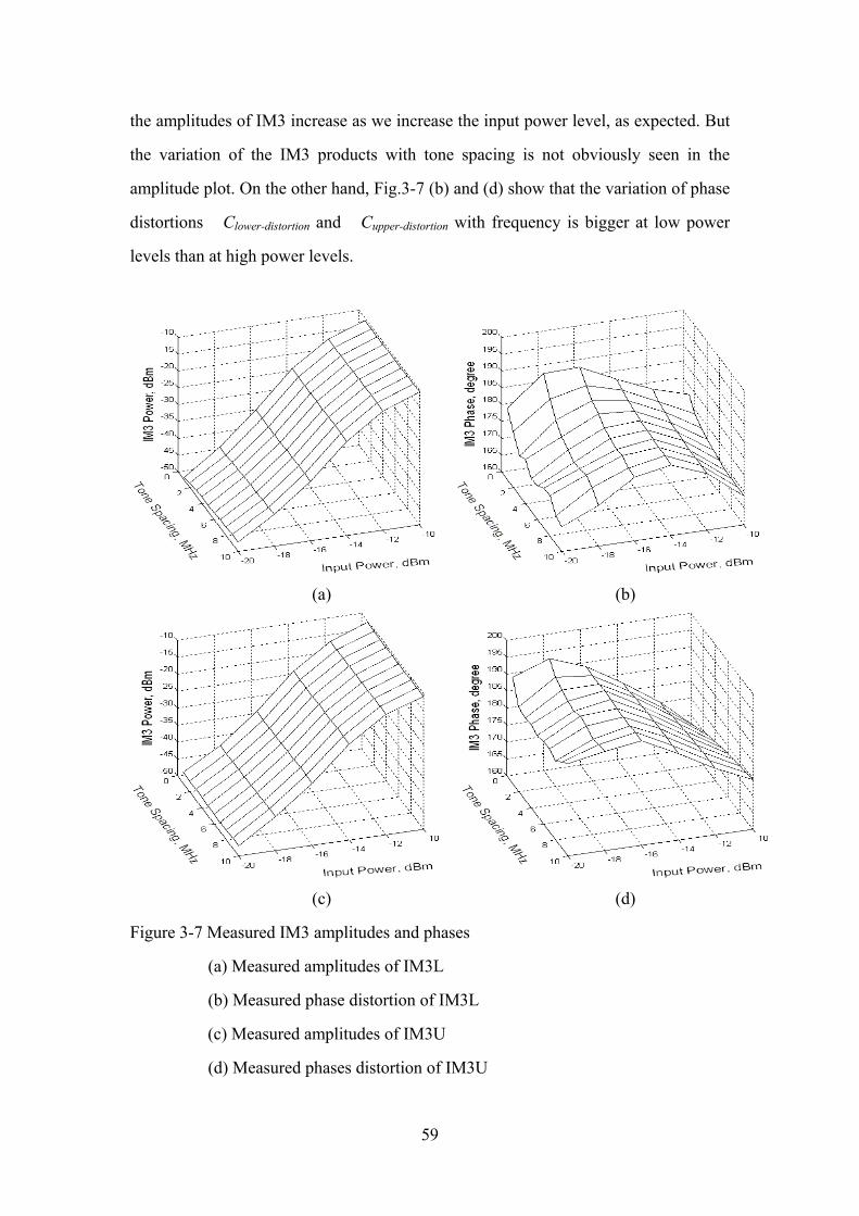
the amplitudes of IM3 increase as we increase the input power level, as expected. But
the variation of the IM3 products with tone spacing is not obviously seen in the
amplitude plot. On the other hand, Fig.3-7 (b) and (d) show that the variation of phase
distortions �Clower-distortion and �Cupper-distortion with frequency is bigger at low power
levels than at high power levels.
(a) (b)
(c) (d)
Figure 3-7 Measured IM3 amplitudes and phases
(a) Measured amplitudes of IM3L
(b) Measured phase distortion of IM3L
(c) Measured amplitudes of IM3U
(d) Measured phases distortion of IM3U
59

3.3.2 Model for single sideband injection
Based on the measurement mentioned previously in Section 3.3.1, this section
proposes a new mathematical description of the relationship between injected IM3L
and output IM3L. The advantage of this mathematical description is that it can clearly
and quickly predict the injection signal required for single sideband predistortion,
instead of tuning the input phase and amplitude manually, or measuring the power
repeatedly. We discuss IM3L injection in detail. The result for IM3U injection
follows analogously.
The input signal is changed to a two-tone with IM3L injection:
( ) ( ) ( )tjektjtjv lowerj
in ωωω expexpexp 1121
Φ++= (3.19)
In (3.19), k1 and Φ1 are used to set the amplitude and phase of the injected IM3L.
We define a new parameter:
( ) ( )LIMInputCCCCC
CjCR lower
referencelower
lowerlower 3
exp 22
1
*2
21÷=
∠=
− (3.20)
Equation (3.20) is similar to (3.18), but with different input signals: (3.18) implies a
two-tone test while (3.20) implies a two-tone test with IM3L injection. This parameter
describes the ratio between output IM3L and reference IM3L. It is simply calculated
from the output phasors at three sub-frequencies C1, C2, Clower.
Figure 3-8 shows different Rlower with respect to different pairs of (k1, Φ1). The dashed
lines indicate contours of constantΦ1, with k1 varying. The solid closed contours
represent constant k1 withΦ1 varying. They are approximately circular.
60

Figure 3-8 Plots of Rlower
We can explain the approximately circular contours in Fig.3-8 by analyzing Clower. It
consists of two parts: the original IM3L produced by two carriers; and the injected
IM3L component multiplied by Glinear-lower, the linear gain of the PA, as shown in
(3.21):
( ) ( )tjekGtjGC lowerj
lowerlinearlowerlowerlower ωω expexp 113
Φ−− ×+×= (3.21)
Equation (3.22) is obtained by substituting (3.21) into the numerator of (3.20):
( ) ( )( )
1
1
13
13
expexpexp
Φ−−
Φ−−
×+=
×+×=
jlowerlinearlower
lower
lowerj
lowerlinearlowerlowerlower
ekGG
tjtjekGtjGR
ωωω
(3.22)
Using (3.22) to interpret Fig.3-8, the centre of these circles is indicated by G3-lower and
the radius is given by Glinear-lower☓k1. The single sideband predistortion can be
61

achieved by choosing appropriate (k1, Φ1) such that (3.22) becomes zero:
lowerlinear
lowerj
GGek
−
−Φ −= 31
1 (3.23)
With the appropriate choice of k1, the circle touches the origin in Fig.3-8 for some
value of Φ1. This corresponds to perfect cancellation. These circles help to explain the
input and output IM3L relation and the meanings of G3-lower, Glinear-lower. In the
predistortion process, we only need two measurements to obtain G3-lower and
Glinear-lower, to determine the required (k1, Φ1) for perfect cancellation. The first one
has k1=0, i.e a two-tone test with no injection, so that Rlower =G3-lower. The second
measurement uses an input two tone signal with IM3L injection using an arbitrary
pair of (k1, Φ1). The Glinear-lower can be calculated from (3.22) using the known (k1, Φ1)
and G3-lower. The measurements need both amplitude and phase, but this predistortion
process is faster than [39].
Similarly, the relation for IM3U and its predistortion are:
( ) ( )
223
122
*1
22 3
expΦ
−−
−
×+=
÷=∠
=
jupperlinearupper
upperreferenceupper
upperupper
ekGG
UIMInputCCCCC
CjC
R (3.24)
upperlinear
upperj
GG
ek−
−Φ −= 32
2 (3.25)
The original two-tone test and these two single sideband predistortion results are
shown in Fig.3-9 (a), (b) and (c).
62
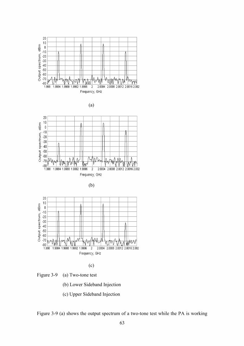
(a)
(b)
(c)
Figure 3-9 (a) Two-tone test
(b) Lower Sideband Injection
(c) Upper Sideband Injection
Figure 3-9 (a) shows the output spectrum of a two-tone test while the PA is working
63
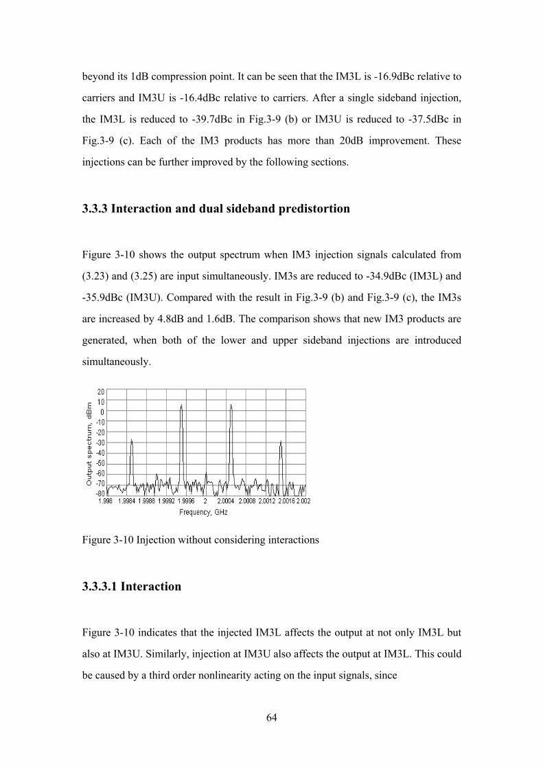
beyond its 1dB compression point. It can be seen that the IM3L is -16.9dBc relative to
carriers and IM3U is -16.4dBc relative to carriers. After a single sideband injection,
the IM3L is reduced to -39.7dBc in Fig.3-9 (b) or IM3U is reduced to -37.5dBc in
Fig.3-9 (c). Each of the IM3 products has more than 20dB improvement. These
injections can be further improved by the following sections.
3.3.3 Interaction and dual sideband predistortion
Figure 3-10 shows the output spectrum when IM3 injection signals calculated from
(3.23) and (3.25) are input simultaneously. IM3s are reduced to -34.9dBc (IM3L) and
-35.9dBc (IM3U). Compared with the result in Fig.3-9 (b) and Fig.3-9 (c), the IM3s
are increased by 4.8dB and 1.6dB. The comparison shows that new IM3 products are
generated, when both of the lower and upper sideband injections are introduced
simultaneously.
Figure 3-10 Injection without considering interactions
3.3.3.1 Interaction
Figure 3-10 indicates that the injected IM3L affects the output at not only IM3L but
also at IM3U. Similarly, injection at IM3U also affects the output at IM3L. This could
be caused by a third order nonlinearity acting on the input signals, since
64
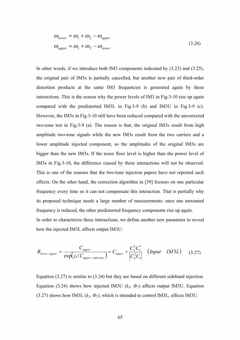
lowerupper
upperlower
ωωωω
ωωωω
−+=
−+=
21
21 (3.26)
In other words, if we introduce both IM3 components indicated by (3.23) and (3.25),
the original pair of IM3s is partially cancelled, but another new pair of third-order
distortion products at the same IM3 frequencies is generated again by these
interactions. This is the reason why the power levels of IM3 in Fig.3-10 rise up again
compared with the predistorted IM3L in Fig.3-9 (b) and IM3U in Fig.3-9 (c).
However, the IM3s in Fig.3-10 still have been reduced compared with the uncorrected
two-tone test in Fig.3-9 (a). The reason is that, the original IM3s result from high
amplitude two-tone signals while the new IM3s result from the two carriers and a
lower amplitude injected component, so the amplitudes of the original IM3s are
bigger than the new IM3s. If the noise floor level is higher than the power level of
IM3s in Fig.3-10, the difference caused by these interactions will not be observed.
This is one of the reasons that the two-tone injection papers have not reported such
effects. On the other hand, the correction algorithm in [39] focuses on one particular
frequency every time so it can not compensate this interaction. That is partially why
its proposed technique needs a large number of measurements: once one unwanted
frequency is reduced, the other predistorted frequency components rise up again.
In order to characterize these interactions, we define another new parameter to reveal
how the injected IM3L affects output IM3U:
( ) ( )LIMInputCCCCC
CjC
R upperreferenceupper
upperupperlower 3
exp 122
*1
22÷=
∠=
−− (3.27)
Equation (3.27) is similar to (3.24) but they are based on different sideband injection.
Equation (3.24) shows how injected IM3U (k2, Ф2) affects output IM3U. Equation
(3.27) shows how IM3L (k1, Ф1), which is intended to control IM3L, affects IM3U.
65

Figure 3-11 shows the measured Rlower-upper with the respect to different pairs of (k1,
Ф1). The dashed lines indicate contours of constant Ф1, with k1 varying. The solid
closed contours represent constant k1 with Ф1 varying. They are approximately
circular like Fig.3-8.
Figure 3-11 Plots of Rlower-upper
Similarly to the lower single sideband injection analysis, we can decompose the
numerator in (3.27) and get:
( )( )[ ]
( )1
121
13
*1
3
expexp
exp
Φ−−−
Φ−
−
−
×+=
⎪⎭
⎪⎬⎫
⎪⎩
⎪⎨⎧
×××+
×
=
jupperlowerupper
upper
lowerjtjtj
upperlower
upperupper
upperlower
ekGG
tjtjekeeG
tjG
Rω
ω
ωωω
(3.28)
where G3-upper is the third-order nonlinearity of the IM3U of the PA, while Glower-upper
is the interaction gain which describes how the input IM3L interacts with the two
carriers to generate another new IM3U contribution through the third-order
nonlinearity of the PA. Because the interaction is contributed by the conjugation of
IM3L, the phase of the second term in (3.28) is negative. Equation (3.28) is similar to
66

(3.22), but the sign of Ф1 is opposite. This can be also observed in the experiments: as
Ф1 increases with constant k1, Rlower in Fig.3-8 rotates anti-clockwise, while Rlower-upper
in Fig.3-11 rotates clockwise. The radius of the circle in Fig.3-11 is much smaller
than the one in Fig.3-8, but it is significant enough to affect dual sideband
predistortion. To the authors knowledge, no paper has proposed this term before. In
the predistortion process, G3-upper is obtained as in the previous section. Glower-upper can
be calculated from one more measurement using any single pair of (k1, Ф1) in (3.28).
By analogy with (3.28), the interaction between the injected IM3U and the carriers,
producing another contribution to IM3L, can be characterized by:
( ) ( )
223
22
1
*2
21 3
expΦ−
−−
−−
×+=
÷=∠
=
jlowerupperlower
lowerreferencelower
lowerlowerupper
ekGG
UIMInputCCCCC
CjCR
(3.29)
3.3.3.2 Dual sideband predistortion
To sum up, the equation for describing dual sideband injected IM3s and output IM3s
considering the interaction is:
( ) ( )( ) (⎪⎩
⎪⎨⎧
++=++=
Φ−−
Φ−−
Φ−−
Φ−−
tjekGekGGCtjekGekGGC
upperj
upperlowerj
upperlinearupperupper
lowerj
lowerupperj
lowerlinearlowerlower
ωω
expexp
12
21
123
213
) (3.30)
When we want to eliminate both IM3s completely at the output using injection, we
need to satisfy this requirement:
0
012
21
123
213
=++
=++Φ−
−Φ
−−
Φ−−
Φ−−
jupperlower
jupperlinearupper
jlowerupper
jlowerlinearlower
ekGekGG
ekGekGG (3.31)
67

It can be organized and re-written in matrix form:
02
1
2
1***
3
3 =⎥⎦
⎤⎢⎣
⎡⎥⎦
⎤⎢⎣
⎡+⎥
⎦
⎤⎢⎣
⎡Φ−
Φ
−−
−−
−
−
j
j
upperlinearupperlower
lowerupperlowerlinear
upper
lower
ekek
GGGG
GG
(3.32)
With the values of Glower, Gupper, Glinear-lower, Glinear-upper, Gupper-lower, Glower-upper
measured in (3.22), (3.24), (3.28) and (3.29), the solution for dual sideband
predistortion would be:
⎥⎦
⎤⎢⎣
⎡⎥⎦
⎤⎢⎣
⎡−=⎥
⎦
⎤⎢⎣
⎡
−
−−
−−
−−
Φ−
Φ
*3
31
**2
12
1
upper
lower
upperlinearupperlower
lowerupperlowerlinearj
j
GG
GGGG
ekek
(3.33)
From this completed matrix description, we can see that perfect dual sideband
predistortion cannot be achieved simply by adding IM3s which have the same
amplitudes but in anti-phase with the original IM3. The trade-off between linear gain
Glinear-lower, Glinear-upper and the interactions Gupper-lower, Glower-upper needs to be
considered as well. Therefore, a complete dual sideband predistortion would be very
hard to optimize by manual tuning.
The parameters for dual sideband predistortion, Glinear-lower, Glinear-upper and Gupper-lower,
Glower-upper are obtained from four measurements. Dual sideband injection using
parameters calculated from Equation (3.33) gives reductions of -38.8dBc for IM3L
and -37.5dBc for IM3U when applied to the same amplifier, as shown in Fig.3-12.
Compared with Fig.3-10, these IM3s have been reduced by 3.9dB (IM3L) and 1.6dB
(IM3U). This injection can be further improved by iterations where both of the IM3s
are reduced to the noise floor, as shown in the next section.
68

Figure 3-12 Measured dual sideband injection predistortion considering interactions
3.3.4 Improvement by iteration
3.3.4.1 Reasons for iteration
There are several issues that affect the accuracies of Glower, Gupper, Glinear-lower,
Glinear-upper, Gupper-lower, Glower-upper:
1) The injected IM3s interact non-linearly with the two carriers. The IM3 references
are constructed from the two carriers. These two aspects will lead to a distortion of
measurement of Rlower, Rupper, Rupper-lower, Rlower-upper and hence affect the calculations
of Glower, Gupper, Glinear-lower, Glinear-upper, Gupper-lower, Glower-upper.
2) The resolution of the DAC in the AMIQ and the ADC in the VSA will generate a
certain degree of inaccuracy which will affect the measurement.
3) The fifth-order nonlinearities will affect the performance as well. Take measuring
Rlower in a single sideband predistortion for example. The input signal can be judged as
a three tone input signal: C1+C2+Clower. There are a lot of fifth-order intermodulation
products generated by the combination of these three carriers. Among these
69
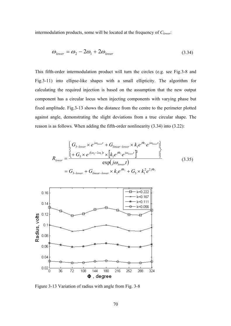
intermodulation products, some will be located at the frequency of Clower:
lowerlower ωωωω 22 12 +−= (3.34)
This fifth-order intermodulation product will turn the circles (e.g. see Fig.3-8 and
Fig.3-11) into ellipse-like shapes with a small ellipticity. The algorithm for
calculating the required injection is based on the assumption that the new output
component has a circular locus when injecting components with varying phase but
fixed amplitude. Fig.3-13 shows the distance from the centre to the perimeter plotted
against angle, demonstrating the slight deviations from a true circular shape. The
reason is as follows. When adding the fifth-order nonlinearity (3.34) into (3.22):
( ) [ ]( )
11
112
1
221513
21
25
13
expΦΦ
−−
Φ−
Φ−−
×+×+=
⎪⎭
⎪⎬⎫
⎪⎩
⎪⎨⎧
××+
×+×
=
jjlowerlinearlower
lower
tjjtj
tjjlowerlinear
tjlower
lower
ekGekGG
tjeekeG
eekGeG
Rlower
lowerlower
ω
ωωω
ωω
(3.35)
Figure 3-13 Variation of radius with angle from Fig. 3-8
70

The relationship between (3.35) and Fig.3-8 is explained as follows:
The first term represents the centre of the circle.
The linear gain Glinear-lower is much bigger than the fifth-order nonlinearity G5. As
a result, the second term determines the average radius while the third term
modulates the radius with two periods per revolution.
The bigger the value of k is in (3.35), the more apparent the radius variation
becomes in Fig.3-13.
This fifth order distortion also affects Rupper, Rupper-lower, Rlower-upper, affecting in turn
the injection accuracy of predistortion in highly nonlinear PAs. They are similar to
Rlower, and we list the frequency relationships in (3.36).
upperlower
lowerupper
upperupper
ωωω
ωωω
ωωωω
23
2322
2
1
21
−=
−=
+−=
(3.36)
The above factors limit the accuracy of calculations for (k1, Φ1) and (k2, Φ2), and
weaken the predistortion as demonstrated by the incomplete cancellation in Fig.3-9
and Fig.3-12.
3.3.4.2 Iteration algorithm and feasibility
In order to demonstrate the feasibility of further improvement by iteration, we discuss
the relation between injected IM3s and output IM3s. Following the format of
Equation (3.32), Equation (3.30) can be written in matrix form:
71

( )
( )⎥⎥⎥⎥
⎦
⎤
⎢⎢⎢⎢
⎣
⎡
−
=⎥⎦
⎤⎢⎣
⎡=Α
⎥⎦
⎤⎢⎣
⎡+⎥
⎦
⎤⎢⎣
⎡=
Φ−
Φ
−−
−−
−
−
tjC
tjC
Bekek
where
AGGGG
GG
B
upper
upper
lower
lower
j
j
upperlinearupperlower
lowerupperlowerlinear
upper
lower
ω
ω
exp
exp2
1
2
1
**3
3
(3.37)
Equation (3.37) describes the transformation from injected IM3s (A) to output IM3s
(B), f: A→B. The linearity of the relationship described by (3.37) should ensure that in
an iterative process, the predistortion result will converge to an optimum. The
iteration steps are:
1. Measure Glower, Gupper, Glinear-lower, Glinear-upper, Gupper-lower, Glower-upper
2. Substitute them into (23) to determine the injection phasors k1ejФ1, k2ejФ2.
3. Change the input signals to:
exp(jω1t)+exp(jω2t) + k1e jΦ1exp(jωlowert)+k2ejΦ2exp(jωuppert)
4. Measure new Glower, Gupper, Glinear-lower, Glinear-upper, Gupper-lower, Glower-upper again.
5. Substitute them into (3.33) and find out new k*1ejФ*1, k*2ejФ*2
6. Add k*1ejФ*1 and k*2ejФ*2 to the injection phasors.
7. Repeat steps 3 to 6 until the IM3 at output is reduced to the noise floor.
3.3.4.3 Experimental results
Figure 3-14 shows single sideband injection in (a) and (b). The improvement, by over
30 dB, between Fig. 3-9 (b) and Fig. 3-14 (a), and between Fig. 3-9 (c) and Fig. 3-14
(b), is brought about by iteration. Using simultaneously the same injection parameters
as in Fig. 3-14 (a) and Fig. 3-14 (b), but without considering interactions, gives the
dual sideband result shown in Fig. 3-14 (c). The result of dual sideband injection,
considering interactions and with 2 iterations is shown in Fig. 3-14 (d). It can be seen
72

that the IM3 can be reduced to around -70dBm, near the noise floor, where further
measurements of Glower, Gupper, Glinear-lower, Glinear-upper, Gupper-lower, Glower-upper for
further iterations become impractical. The dual sideband injection predistortion in Fig.
3-14 (d) has reduced IM3s by 60dB compared with the original two-tone test output
spectrum in Fig. 3-9 (a).
(a)
(b)
73
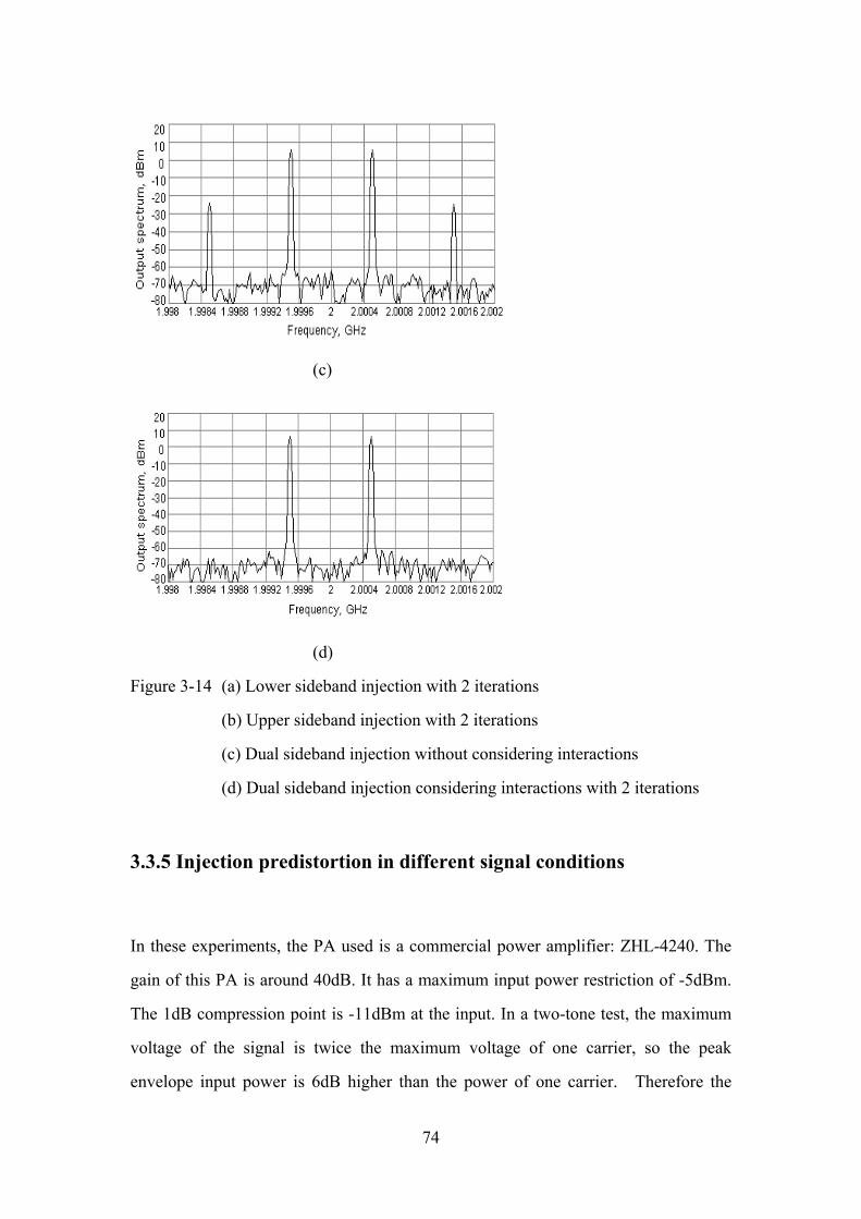
(c)
(d)
Figure 3-14 (a) Lower sideband injection with 2 iterations
(b) Upper sideband injection with 2 iterations
(c) Dual sideband injection without considering interactions
(d) Dual sideband injection considering interactions with 2 iterations
3.3.5 Injection predistortion in different signal conditions
In these experiments, the PA used is a commercial power amplifier: ZHL-4240. The
gain of this PA is around 40dB. It has a maximum input power restriction of -5dBm.
The 1dB compression point is -11dBm at the input. In a two-tone test, the maximum
voltage of the signal is twice the maximum voltage of one carrier, so the peak
envelope input power is 6dB higher than the power of one carrier. Therefore the
74
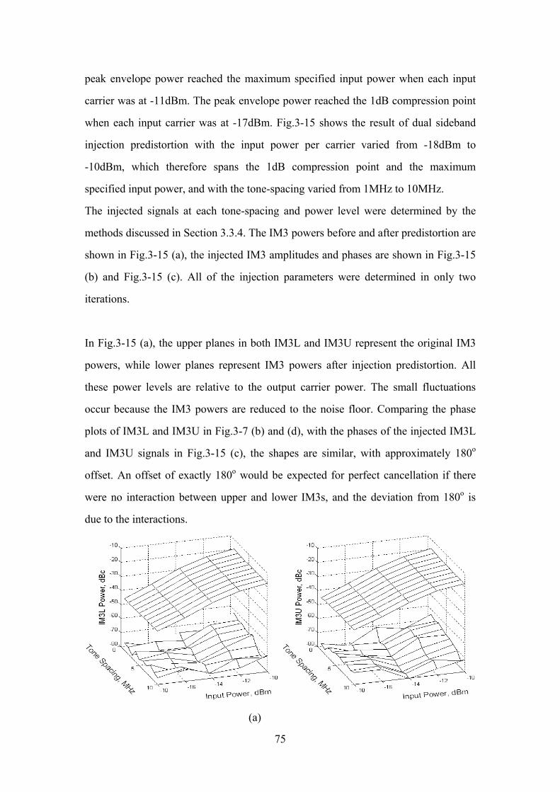
peak envelope power reached the maximum specified input power when each input
carrier was at -11dBm. The peak envelope power reached the 1dB compression point
when each input carrier was at -17dBm. Fig.3-15 shows the result of dual sideband
injection predistortion with the input power per carrier varied from -18dBm to
-10dBm, which therefore spans the 1dB compression point and the maximum
specified input power, and with the tone-spacing varied from 1MHz to 10MHz.
The injected signals at each tone-spacing and power level were determined by the
methods discussed in Section 3.3.4. The IM3 powers before and after predistortion are
shown in Fig.3-15 (a), the injected IM3 amplitudes and phases are shown in Fig.3-15
(b) and Fig.3-15 (c). All of the injection parameters were determined in only two
iterations.
In Fig.3-15 (a), the upper planes in both IM3L and IM3U represent the original IM3
powers, while lower planes represent IM3 powers after injection predistortion. All
these power levels are relative to the output carrier power. The small fluctuations
occur because the IM3 powers are reduced to the noise floor. Comparing the phase
plots of IM3L and IM3U in Fig.3-7 (b) and (d), with the phases of the injected IM3L
and IM3U signals in Fig.3-15 (c), the shapes are similar, with approximately 180o
offset. An offset of exactly 180o would be expected for perfect cancellation if there
were no interaction between upper and lower IM3s, and the deviation from 180o is
due to the interactions.
(a)
75
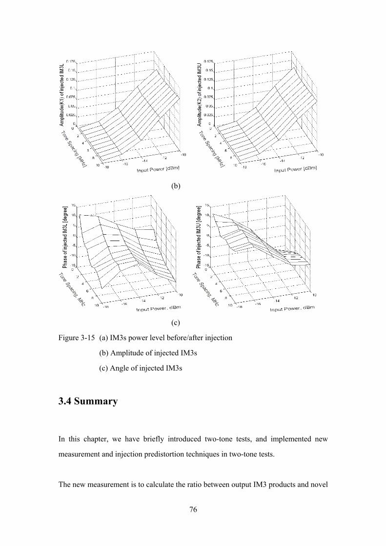
(b)
(c)
Figure 3-15 (a) IM3s power level before/after injection
(b) Amplitude of injected IM3s
(c) Angle of injected IM3s
3.4 Summary
In this chapter, we have briefly introduced two-tone tests, and implemented new
measurement and injection predistortion techniques in two-tone tests.
The new measurement is to calculate the ratio between output IM3 products and novel
76

IM3 references which are created by the two main output tones. With these results, we
can clearly describe the relationship between injected and output IM3 products. Based
on this relationship, a correct injection for either lower or upper sideband IM3 can be
easily calculated instead of manual tuning. Additionally, interaction between lower
and upper sideband IM3 products has been revealed during the research. To our
knowledge, this interaction has not been proposed in published papers before. As a
result, further IM3 reductions have been achieved considering these interactions. The
advantage of injection compared with a look-up table approach is that it can address
each intermodulation product separately, making it more capable of handling memory
effects in PAs.
77

CHAPTER 4
APPLICATION OF INJECTION PREDISTORTION TECHNIQUES IN 16 QAM
SIGNALS After applying injection predistortion in two-tone tests in Chapter 3, here we will
apply the similar methods to a PA subjected to a 16 QAM signals. In this chapter, we
will firstly review the injection results in the published papers, and then introduce our
different injection techniques. Furthermore, we will demonstrate how this injection
predistortion deals with memory effects.
4.1 Published injection predistortion result for wideband
signal
Since injection linearization has been proved to work in two-tone tests, it is
reasonable to apply similar techniques in a PA subjected to 16 QAM signals. The
principles are explained in Chapter 2, so in this section, we just review their
performances.
Paper [48] has shown a harmonic injection technique applied to a 28 dBm PA with a
1.23 MHz channel bandwidth offset-QPSK CDMA signal, in Fig. 4-1. An average
improvement in adjacent channel power ratio (ACPR) of 6 dB is obtained.
78
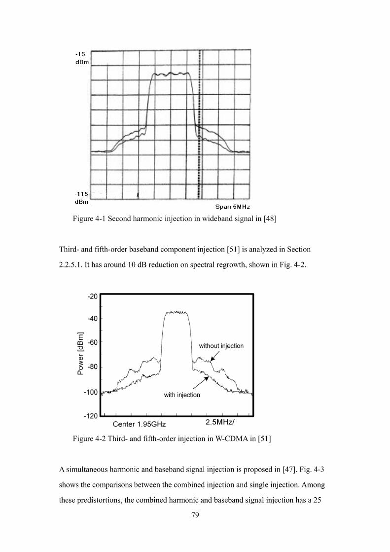
Figure 4-1 Second harmonic injection in wideband signal in [48]
Third- and fifth-order baseband component injection [51] is analyzed in Section
2.2.5.1. It has around 10 dB reduction on spectral regrowth, shown in Fig. 4-2.
Figure 4-2 Third- and fifth-order injection in W-CDMA in [51]
A simultaneous harmonic and baseband signal injection is proposed in [47]. Fig. 4-3
shows the comparisons between the combined injection and single injection. Among
these predistortions, the combined harmonic and baseband signal injection has a 25
79
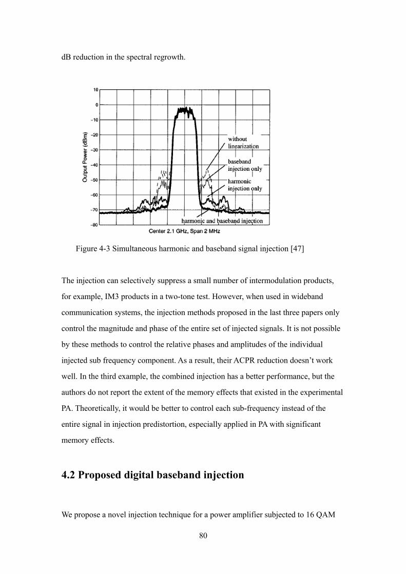
dB reduction in the spectral regrowth.
Figure 4-3 Simultaneous harmonic and baseband signal injection [47]
The injection can selectively suppress a small number of intermodulation products,
for example, IM3 products in a two-tone test. However, when used in wideband
communication systems, the injection methods proposed in the last three papers only
control the magnitude and phase of the entire set of injected signals. It is not possible
by these methods to control the relative phases and amplitudes of the individual
injected sub frequency component. As a result, their ACPR reduction doesn’t work
well. In the third example, the combined injection has a better performance, but the
authors do not report the extent of the memory effects that existed in the experimental
PA. Theoretically, it would be better to control each sub-frequency instead of the
entire signal in injection predistortion, especially applied in PA with significant
memory effects.
4.2 Proposed digital baseband injection
We propose a novel injection technique for a power amplifier subjected to 16 QAM
80
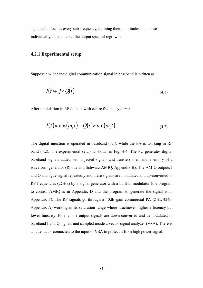
signals. It allocates every sub-frequency, defining their amplitudes and phases
individually, to counteract the output spectral regrowth.
4.2.1 Experimental setup
Suppose a wideband digital communication signal in baseband is written as
( ) ( )tQjtI ×+ (4.1)
After modulation in RF domain with centre frequency of ωc:
( ) ( ) ( ) ( )ttQttI cc ωω sincos ×−× (4.2)
The digital injection is operated in baseband (4.1), while the PA is working in RF
band (4.2). The experimental setup is shown in Fig. 4-4. The PC generates digital
baseband signals added with injected signals and transfers them into memory of a
waveform generator (Rhode and Schwarz AMIQ, Appendix B). The AMIQ outputs I
and Q analogue signal repeatedly and these signals are modulated and up-converted to
RF frequencies (2GHz) by a signal generator with a built-in modulator (the program
to control AMIQ is in Appendix D and the program to generate the signal is in
Appendix F). The RF signals go through a 40dB gain commercial PA (ZHL-4240,
Appendix A) working in its saturation range where it achieves higher efficiency but
lower linearity. Finally, the output signals are down-converted and demodulated to
baseband I and Q signals and sampled inside a vector signal analyzer (VSA). There is
an attenuator connected to the input of VSA to protect it from high power signal.
81
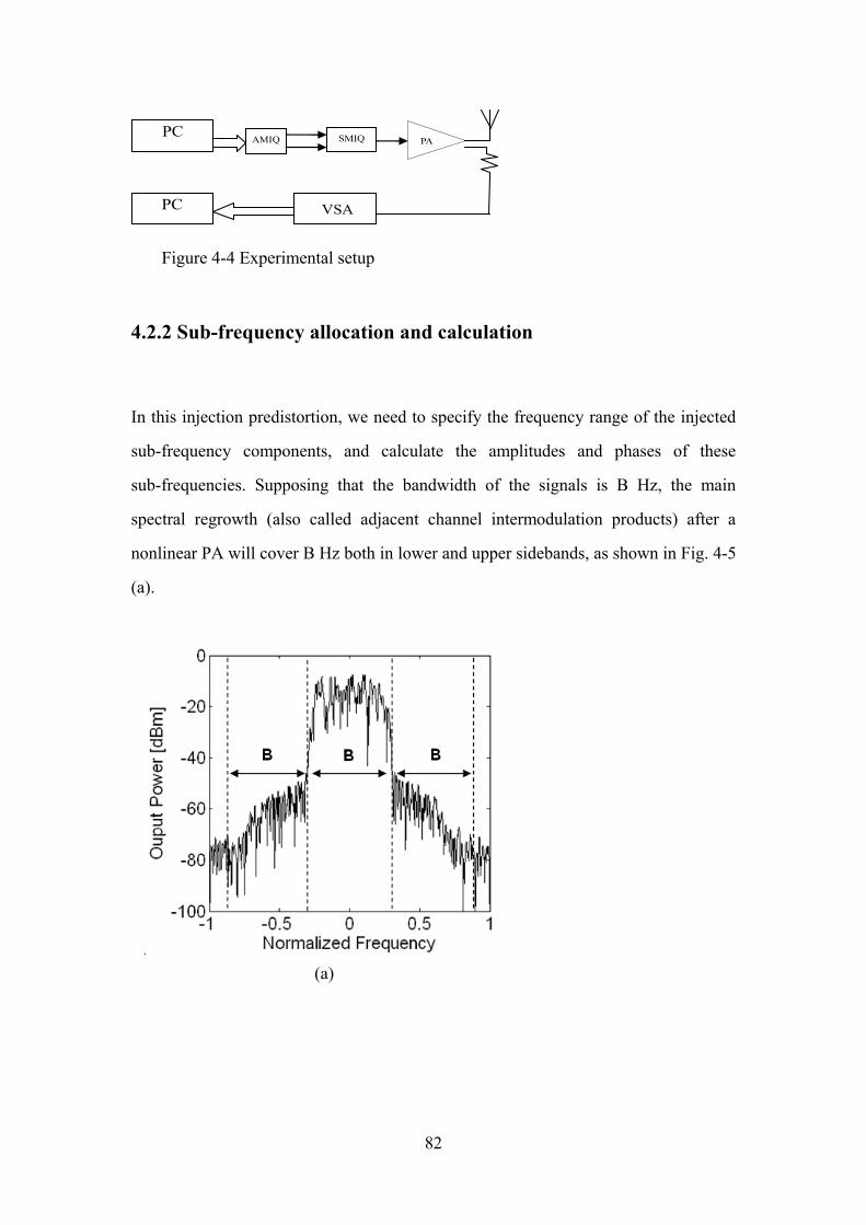
PC
AMIQ PA
VSA
SMIQ
PC
Figure 4-4 Experimental setup
4.2.2 Sub-frequency allocation and calculation
In this injection predistortion, we need to specify the frequency range of the injected
sub-frequency components, and calculate the amplitudes and phases of these
sub-frequencies. Supposing that the bandwidth of the signals is B Hz, the main
spectral regrowth (also called adjacent channel intermodulation products) after a
nonlinear PA will cover B Hz both in lower and upper sidebands, as shown in Fig. 4-5
(a).
(a)
82
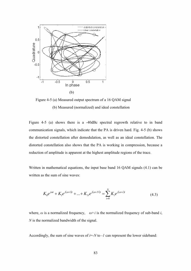
(b)
Figure 4-5 (a) Measured output spectrum of a 16 QAM signal
(b) Measured (normalized) and ideal constellation
Figure 4-5 (a) shows there is a -40dBc spectral regrowth relative to in band
communication signals, which indicate that the PA is driven hard. Fig. 4-5 (b) shows
the distorted constellation after demodulation, as well as an ideal constellation. The
distorted constellation also shows that the PA is working in compression, because a
reduction of amplitude is apparent at the highest amplitude regions of the trace.
Written in mathematical equations, the input base band 16 QAM signals (4.1) can be
written as the sum of sine waves:
( ) ( ) ( )∑=
+++ =+++N
i
tiji
tNjN
tjtj eKeKeKeK0
110 ... ωωωω
(4.3)
where, ω is a normalized frequency, ω+i is the normalized frequency of sub-band i,
N is the normalized bandwidth of the signal.
Accordingly, the sum of sine waves of i=-N to -1 can represent the lower sideband:
83

( ) ( ) ( ) ( )∑−
−=
+−−
−−
−− =+++
12
21
1Ni
tiji
tNjN
tjtj eKeKeKeK ωωωω K (4.4)
Similarly, the upper sideband spectral regrowth with sub-frequencies of i=N+1 to 2N
would be:
( ) ( ) ( ) (∑+
+++++
+++ =+++
N
N
tiji
tNjN
tNjN
tNjN eKeKeKeK
2
1
22
22
11
ωωωω K ) (4.5)
The aim of injection predistortion is to choose appropriate values of K in (4.4) and
(4.5), to counteract the output spectral regrowth. We define 10 groups of K values,
shown in table 4-1. Each row in table 4-1 represents a set of experimental K values.
And each set of K values will be applied to (4.4) and (4.5) as an injected signal to go
through the PA. So we have ten output results.
TABLE 4-1 Values for K
K-N … K-2 K-1 KN+1 KN+2 … K2N
1 π51j
e π51j
e π51j
e π
51j
e π
51j
e π
51j
e π
51j
e π
51j
e 2 π
52j
e π
52j
e π
52j
e π
52j
e π
52j
e π
52j
e π
52j
e π
52j
e … π
541j
eπ
541j
e π
541j
e π
541j
eπ
541j
eπ
541j
eπ
541j
eπ
541j
e
10 π2je π2je π2je π2je π2je π2je π2je π2je
In our experiment, we are using 16-QAM modulations to encode a sequence of 50
symbols repeatedly, with a raised cosine filter with an up sample rate of 10. Thus each
period of 50 symbols has 500 samples. When we apply a Fourier transform on one
period of these signals, there are 500 different sub-frequencies in frequency domain.
The wanted signal covers sub-frequencies from -29 to 30 as shown in Fig. 4-6 (a).
84
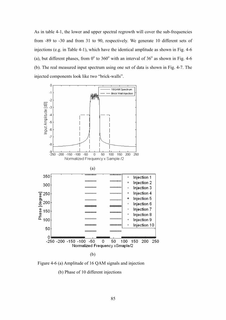
As in table 4-1, the lower and upper spectral regrowth will cover the sub-frequencies
from -89 to -30 and from 31 to 90, respectively. We generate 10 different sets of
injections (e.g. in Table 4-1), which have the identical amplitude as shown in Fig. 4-6
(a), but different phases, from 0o to 360o with an interval of 36o as shown in Fig. 4-6
(b). The real measured input spectrum using one set of data is shown in Fig. 4-7. The
injected components look like two “brick-walls”.
(a)
(b)
Figure 4-6 (a) Amplitude of 16 QAM signals and injection
(b) Phase of 10 different injections
85
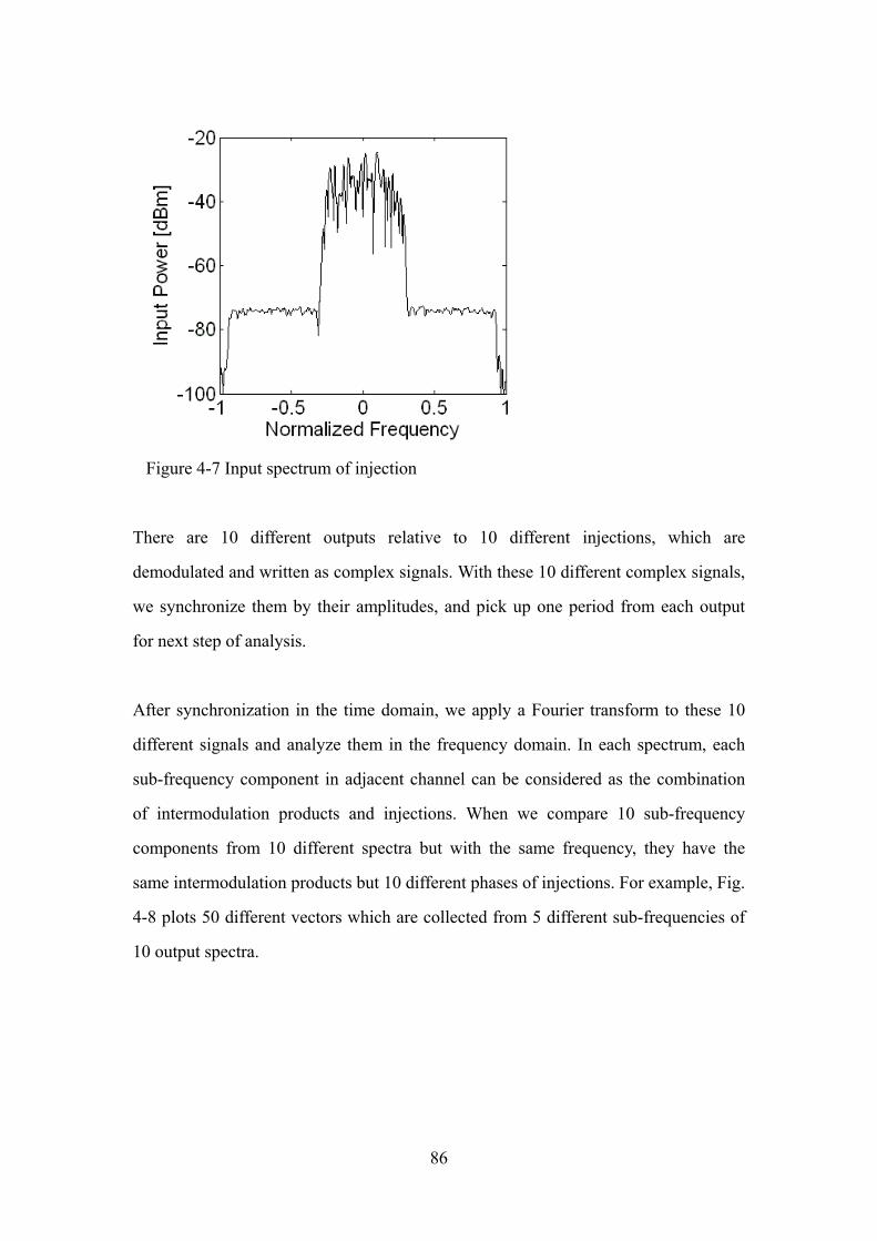
Figure 4-7 Input spectrum of injection
There are 10 different outputs relative to 10 different injections, which are
demodulated and written as complex signals. With these 10 different complex signals,
we synchronize them by their amplitudes, and pick up one period from each output
for next step of analysis.
After synchronization in the time domain, we apply a Fourier transform to these 10
different signals and analyze them in the frequency domain. In each spectrum, each
sub-frequency component in adjacent channel can be considered as the combination
of intermodulation products and injections. When we compare 10 sub-frequency
components from 10 different spectra but with the same frequency, they have the
same intermodulation products but 10 different phases of injections. For example, Fig.
4-8 plots 50 different vectors which are collected from 5 different sub-frequencies of
10 output spectra.
86
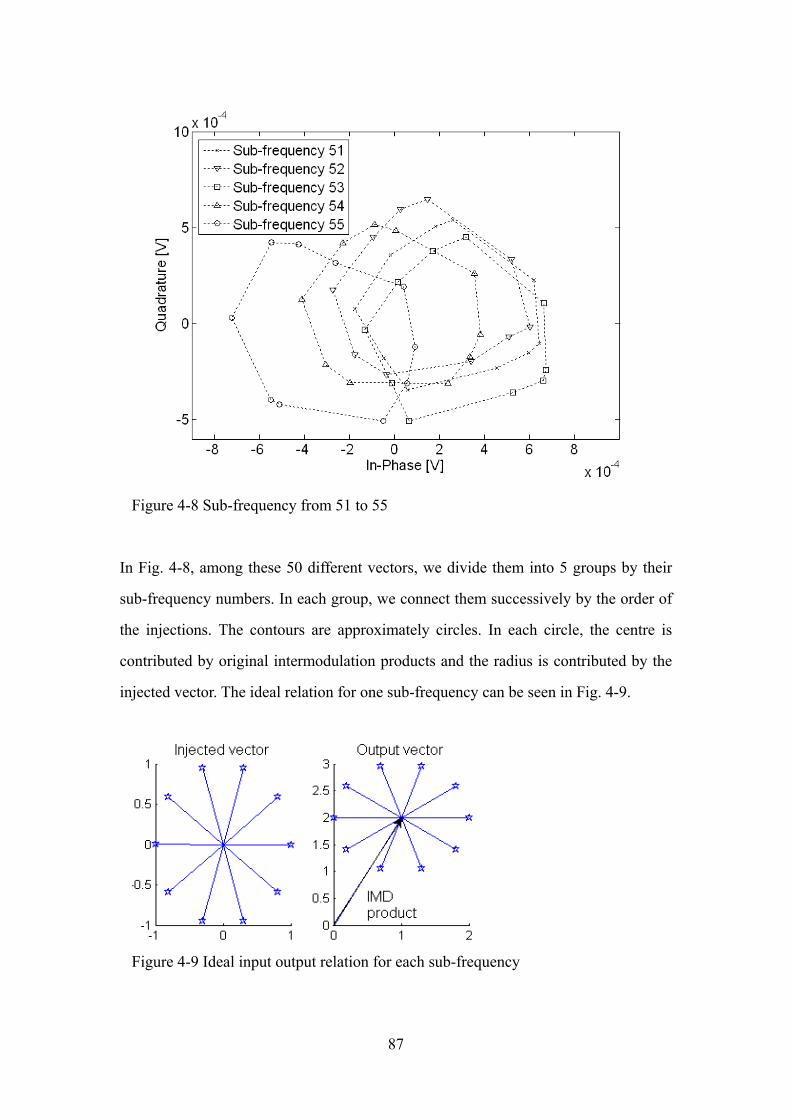
Figure 4-8 Sub-frequency from 51 to 55
In Fig. 4-8, among these 50 different vectors, we divide them into 5 groups by their
sub-frequency numbers. In each group, we connect them successively by the order of
the injections. The contours are approximately circles. In each circle, the centre is
contributed by original intermodulation products and the radius is contributed by the
injected vector. The ideal relation for one sub-frequency can be seen in Fig. 4-9.
Figure 4-9 Ideal input output relation for each sub-frequency
87

The target for the injection is to generate a new vector which counteracts the original
intermodulation products at every sub-frequency in the lower and upper side band.
Note that the interactions in two-tone test injection also occur in the wideband signal
injection. These can be observed by the distortions of the circles in Fig. 4-8. The
equation for solving interactions in two-tone tests is written again here:
⎥⎦
⎤⎢⎣
⎡⎥⎦
⎤⎢⎣
⎡−=⎥
⎦
⎤⎢⎣
⎡
−
−−
−−
−−
Φ−
Φ
*3
31
**2
12
1
upper
lower
upperlinearupperlower
lowerupperlowerlinearj
j
GG
GGGG
ekek
(3.33)
A 2☓2 matrix with 4 parameters is simple and effective for a two-tone test. However,
when this matrix is applied to a wideband signal case, its size will increase
dramatically. For example, there are 120 sub-frequencies in this 16 QAM signal,
which indicates a 120☓120 matrix. For each element of this matrix, we need to plot a
circle to calculate its value. Even though we can measure 3 spots to identify the circle
as the fastest way, there are still totally 120☓120☓3=43200 measurements to
complete this matrix. This matrix method is unrealistic in wide band signal cases.
Therefore, an alternative is needed.
In this case, we propose an iterative method to solve this interaction problem in
wideband signal cases. Suppose the total number of sub-frequencies of the QAM
signal is N, which means:
( ) ( ) ( )∑=
+=+N
i
tijieKtjQtI
0
ω (4.6)
It also means that each of the lower and upper sideband spectral regrowth has N
sub-frequencies, which is coordinate with (4.3), (4.4) and (4.5). With these
assumptions, the iteration is shown and explained as follows:
88
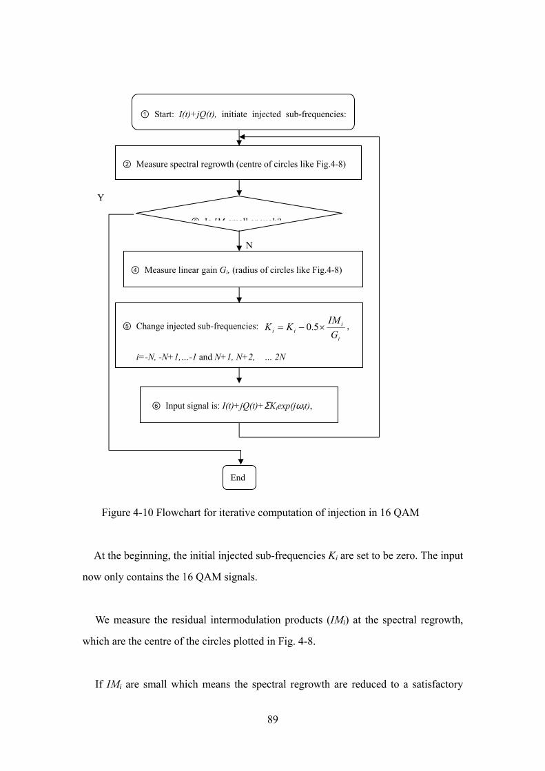
① Start: I(t)+jQ(t), initiate injected sub-frequencies:
② Measure spectral regrowth (centre of circles like Fig.4-8)
③ Is IM small enough?
N
④ Measure linear gain Gi, (radius of circles like Fig.4-8)
⑤ Change injected sub-frequencies: i
iii G
IMKK ×−= 5.0 ,
i=-N, -N+1,…-1 and N+1, N+2, … 2N
⑥ Input signal is: I(t)+jQ(t)+ΣKiexp(jωit),
Y
End
Figure 4-10 Flowchart for iterative computation of injection in 16 QAM
� At the beginning, the initial injected sub-frequencies Ki are set to be zero. The input
now only contains the 16 QAM signals.
� We measure the residual intermodulation products (IMi) at the spectral regrowth,
which are the centre of the circles plotted in Fig. 4-8.
� If IMi are small which means the spectral regrowth are reduced to a satisfactory
89

range, we stop the process, otherwise we begin to calculate the injection Ki.
� We measure the linear gain of the PA (Gi), at different sub-frequencies, which can
be determined from the radius of the circles in Fig. 4-8. The linear gains should be
identical in a memoryless PA case. However, in a PA with memory effects, they vary
with frequency, so we need to measure them separately.
� The injection without considering the interaction would be:
i
ii G
IMK −= (4.7)
We put a negative sign in (4.7) because we need the opposite phases for injection.
When (4.7) is applied to the procedure, we have two modifications. Firstly, a
reduction to the injected components is needed in order to suppress the interaction
between the in band signal and these injected components. In this case, we divide all
the injected components by two. However, this suppression coefficient can be varied
from zero to one, depending on the situation. For example, we can have a smaller
coefficient if the interactions are substantial, or have a larger coefficient if the
interactions are inconspicuous. Secondly, all of the injection results are accumulated
in the iteration. So (4.7) is changed to:
i
iii G
IMKnewK ×−= 5.0)( (4.8)
� All the injected sub-frequencies and the 16 QAM signal are added together as a
new input signal. We then go to step � again.
90
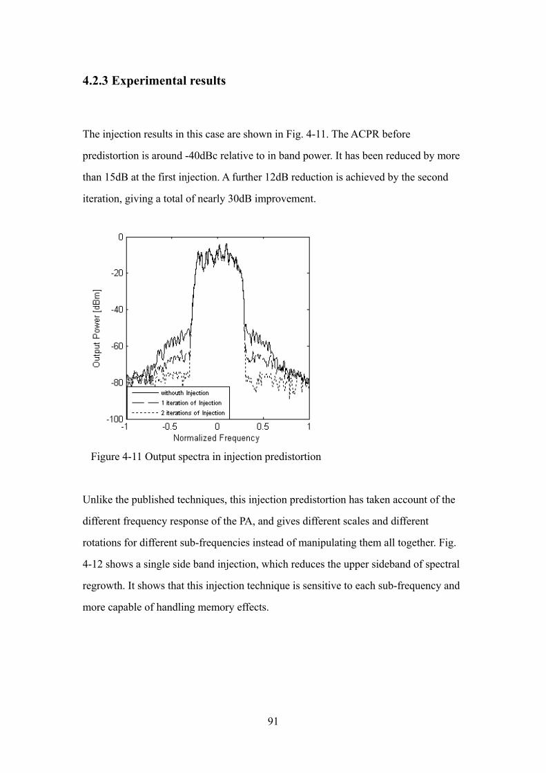
4.2.3 Experimental results
The injection results in this case are shown in Fig. 4-11. The ACPR before
predistortion is around -40dBc relative to in band power. It has been reduced by more
than 15dB at the first injection. A further 12dB reduction is achieved by the second
iteration, giving a total of nearly 30dB improvement.
Figure 4-11 Output spectra in injection predistortion
Unlike the published techniques, this injection predistortion has taken account of the
different frequency response of the PA, and gives different scales and different
rotations for different sub-frequencies instead of manipulating them all together. Fig.
4-12 shows a single side band injection, which reduces the upper sideband of spectral
regrowth. It shows that this injection technique is sensitive to each sub-frequency and
more capable of handling memory effects.
91

Figure 4-12 Upper sideband injection
4.3 Summary
In this chapter, we have applied the similar digital injection techniques to a 16 QAM
wideband signal. Since the matrix approach is no longer practical in wideband signal
cases, we use an iterative method to solve the interaction problem.
Unlike the published injection techniques, this new digital injection predistortion
method can address the amplitude and phase for each sub-frequency in the spectral
regrowth. In our experiment, this injection technique achieves a 30 dB reduction of
spectral regrowth, which is better than the published papers. Additionally, we have
also proved that this injection method can suppress the upper and lower spectral
regrowth sidebands separately, thus demonstrating its capacity for dealing with
memory effects.
It is easy to reduce the spectral regrowth by suppressing them to zero. However, it is
more difficult to tell the correct values of amplitudes and phases of the
92

sub-frequencies in the in band range. Therefore, this injection technique can not
reduce intermodulation products in the in band signal. Additionally, the interactions
caused by the injected signal will be added to the in band signal. In Chapter 5, we will
propose a combined technique, which can solve this problem.
93
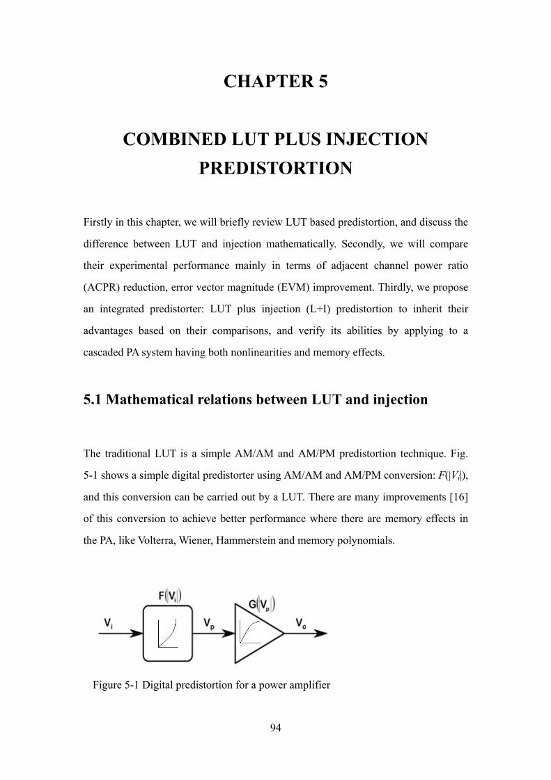
CHAPTER 5
COMBINED LUT PLUS INJECTION PREDISTORTION
Firstly in this chapter, we will briefly review LUT based predistortion, and discuss the
difference between LUT and injection mathematically. Secondly, we will compare
their experimental performance mainly in terms of adjacent channel power ratio
(ACPR) reduction, error vector magnitude (EVM) improvement. Thirdly, we propose
an integrated predistorter: LUT plus injection (L+I) predistortion to inherit their
advantages based on their comparisons, and verify its abilities by applying to a
cascaded PA system having both nonlinearities and memory effects.
5.1 Mathematical relations between LUT and injection
The traditional LUT is a simple AM/AM and AM/PM predistortion technique. Fig.
5-1 shows a simple digital predistorter using AM/AM and AM/PM conversion: F(|Vi|),
and this conversion can be carried out by a LUT. There are many improvements [16]
of this conversion to achieve better performance where there are memory effects in
the PA, like Volterra, Wiener, Hammerstein and memory polynomials.
Figure 5-1 Digital predistortion for a power amplifier
94
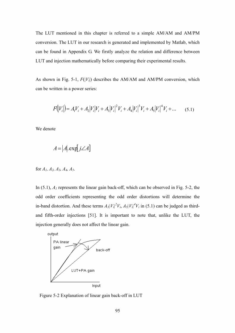
The LUT mentioned in this chapter is referred to a simple AM/AM and AM/PM
conversion. The LUT in our research is generated and implemented by Matlab, which
can be found in Appendix G. We firstly analyze the relation and difference between
LUT and injection mathematically before comparing their experimental results.
As shown in Fig. 5-1, F(|Vi|) describes the AM/AM and AM/PM conversion, which
can be written in a power series:
( ) ...45
34
2321 +++++= iiiiiiiiii VVAVVAVVAVVAVAVF (5.1)
We denote
[ ]AjAA ∠= exp.
for A1, A2, A3, A4, A5.
In (5.1), A1 represents the linear gain back-off, which can be observed in Fig. 5-2, the
odd order coefficients representing the odd order distortions will determine the
in-band distortion. And these terms A3|Vi|2Vi, A5|Vi|4Vi in (5.1) can be judged as third-
and fifth-order injections [51]. It is important to note that, unlike the LUT, the
injection generally does not affect the linear gain.
Figure 5-2 Explanation of linear gain back-off in LUT
95

We now analyze the differences among LUT, published injection and our proposed
injection techniques.
Assume that the input Vi is written in the form of Fourier series as:
( ) ( ) ( )∑=
+++ =+++N
i
tiji
tNjN
tjtj eKeKeKeK0
110 ... ωωωω
(5.2)
Equation (5.2) is the same as (4.3). The third-order power series of LUT, (i.e.,
A3|Vi|2Vi) would be:
( ) ( )( )
( ) ( )( )tNjN
tjtj
tNjN
tjtjii
eKeKeK
eKeKeKAVVA+−+−−
++
+++
×+++=ωωω
ωωω
...
...1
10
21103
*23 (5.3)
There will be a lot of cross products in (5.3). Disregarding the coefficients A and K,
and focusing on the exponential terms, we will find out that:
( ) ( )( ) ( )
( ) ( ) ( ) tjtNjtNj
tjtNjtNjtjtj
eeeeeeee
11
11 ...−+−−
+−−++
+++=
××+++ωωω
ωωωωω
L (5.4)
These cross products will provide the lower sideband frequencies, the same as in (4.4).
And we can find out the upper sideband frequencies in (5.3) similarly:
( ) ( ) ( )( ) ( )
( ) ( ) ( ) tNjtNjtNj
tNjtjtNjtjtj
eeeeeeee
221
21 ...+++++
+−+++
+++=
××+++ωωω
ωωωωω
L (5.5)
In other words, this third-order term has provided us both of the lower and upper
sideband frequencies. The published injection [47, 48, 51] and LUT focus on
verifying A3, which is enough while the PA doesn’t have strong memory effects. By
contrast, our injection focuses on the lower and upper sideband of the sub-frequencies
96
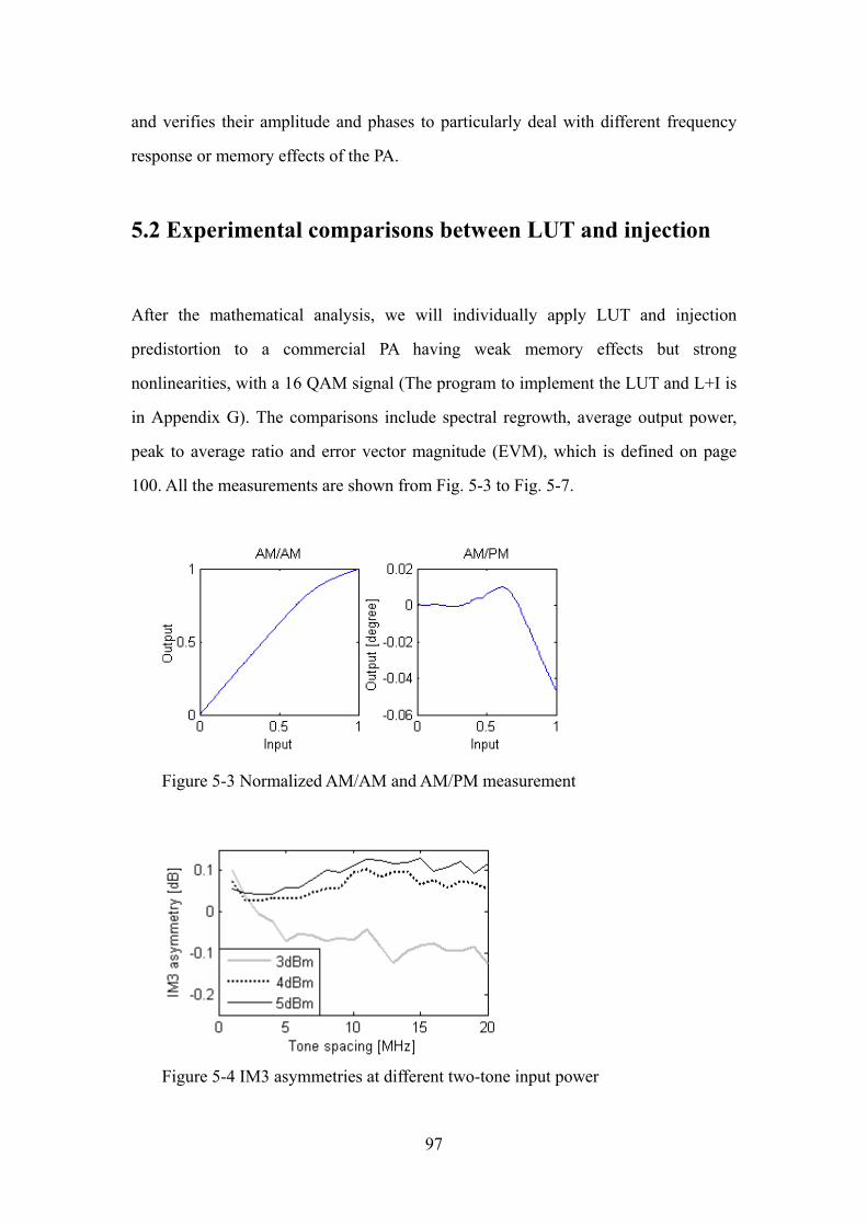
and verifies their amplitude and phases to particularly deal with different frequency
response or memory effects of the PA.
5.2 Experimental comparisons between LUT and injection
After the mathematical analysis, we will individually apply LUT and injection
predistortion to a commercial PA having weak memory effects but strong
nonlinearities, with a 16 QAM signal (The program to implement the LUT and L+I is
in Appendix G). The comparisons include spectral regrowth, average output power,
peak to average ratio and error vector magnitude (EVM), which is defined on page
100. All the measurements are shown from Fig. 5-3 to Fig. 5-7.
Figure 5-3 Normalized AM/AM and AM/PM measurement
Figure 5-4 IM3 asymmetries at different two-tone input power
97
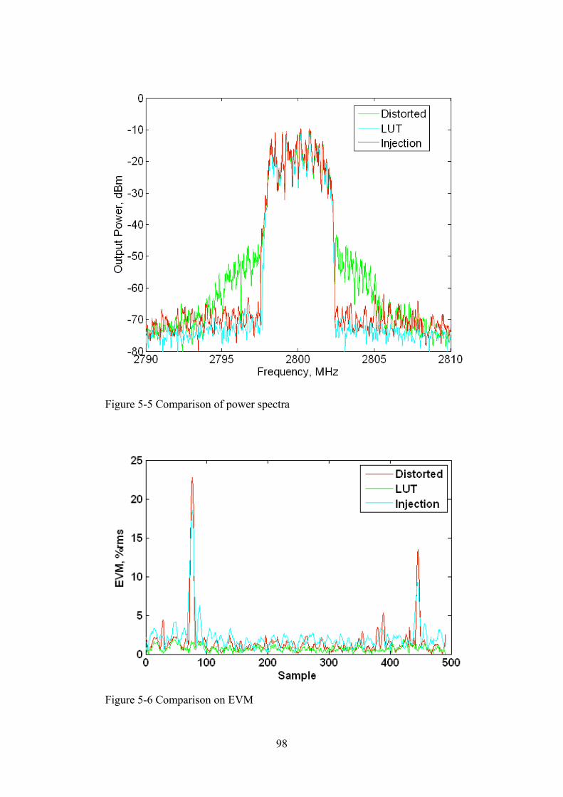
Figure 5-5 Comparison of power spectra
Figure 5-6 Comparison on EVM
98
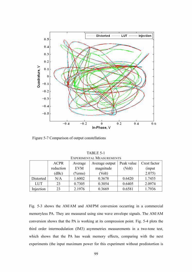
Figure 5-7 Comparison of output constellations
TABLE 5-1 EXPERIMENTAL MEASUREMENTS
ACPR reduction
(dBc)
Average EVM
Average output magnitude
(Volt)
Peak value (Volt)
Crest factor (input 2.075) (%rms)
Distorted N/A 1.6002
0.3678 0.6420 1.7455 LUT 23 0.7305 0.3054 0.6405 2.0974
Injection 23 2.1976
0.3669 0.6581 1.7936
Fig. 5-3 shows the AM/AM and AM/PM conversion occurring in a commercial
memoryless PA. They are measured using sine wave envelope signals. The AM/AM
conversion shows that the PA is working at its compression point. Fig. 5-4 plots the
third order intermodulation (IM3) asymmetries measurements in a two-tone test,
which shows that the PA has weak memory effects, comparing with the next
experiments (the input maximum power for this experiment without predistortion is
99
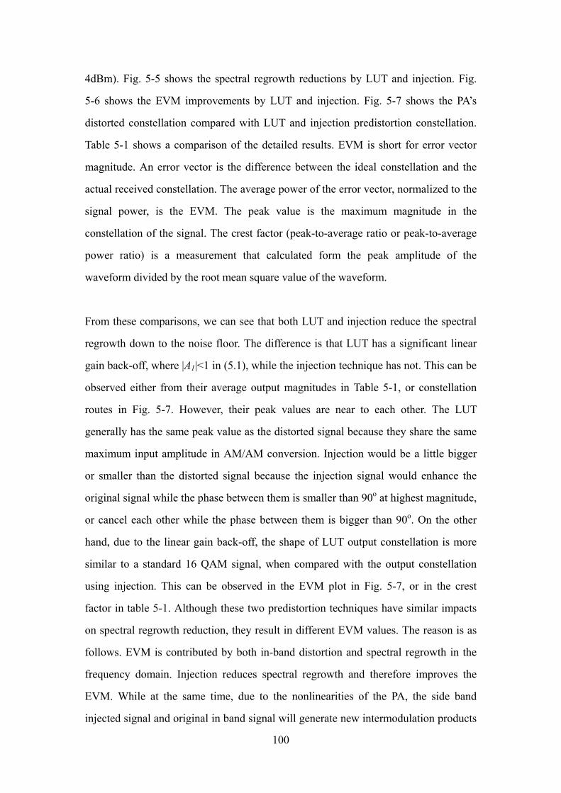
4dBm). Fig. 5-5 shows the spectral regrowth reductions by LUT and injection. Fig.
5-6 shows the EVM improvements by LUT and injection. Fig. 5-7 shows the PA’s
distorted constellation compared with LUT and injection predistortion constellation.
Table 5-1 shows a comparison of the detailed results. EVM is short for error vector
magnitude. An error vector is the difference between the ideal constellation and the
actual received constellation. The average power of the error vector, normalized to the
signal power, is the EVM. The peak value is the maximum magnitude in the
constellation of the signal. The crest factor (peak-to-average ratio or peak-to-average
power ratio) is a measurement that calculated form the peak amplitude of the
waveform divided by the root mean square value of the waveform.
From these comparisons, we can see that both LUT and injection reduce the spectral
regrowth down to the noise floor. The difference is that LUT has a significant linear
gain back-off, where |A1|<1 in (5.1), while the injection technique has not. This can be
observed either from their average output magnitudes in Table 5-1, or constellation
routes in Fig. 5-7. However, their peak values are near to each other. The LUT
generally has the same peak value as the distorted signal because they share the same
maximum input amplitude in AM/AM conversion. Injection would be a little bigger
or smaller than the distorted signal because the injection signal would enhance the
original signal while the phase between them is smaller than 90o at highest magnitude,
or cancel each other while the phase between them is bigger than 90o. On the other
hand, due to the linear gain back-off, the shape of LUT output constellation is more
similar to a standard 16 QAM signal, when compared with the output constellation
using injection. This can be observed in the EVM plot in Fig. 5-7, or in the crest
factor in table 5-1. Although these two predistortion techniques have similar impacts
on spectral regrowth reduction, they result in different EVM values. The reason is as
follows. EVM is contributed by both in-band distortion and spectral regrowth in the
frequency domain. Injection reduces spectral regrowth and therefore improves the
EVM. While at the same time, due to the nonlinearities of the PA, the side band
injected signal and original in band signal will generate new intermodulation products
100
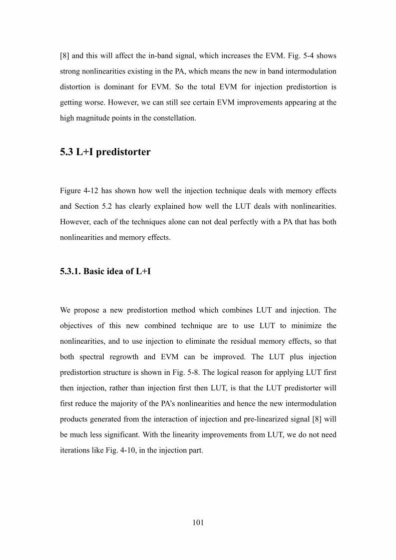
[8] and this will affect the in-band signal, which increases the EVM. Fig. 5-4 shows
strong nonlinearities existing in the PA, which means the new in band intermodulation
distortion is dominant for EVM. So the total EVM for injection predistortion is
getting worse. However, we can still see certain EVM improvements appearing at the
high magnitude points in the constellation.
5.3 L+I predistorter
Figure 4-12 has shown how well the injection technique deals with memory effects
and Section 5.2 has clearly explained how well the LUT deals with nonlinearities.
However, each of the techniques alone can not deal perfectly with a PA that has both
nonlinearities and memory effects.
5.3.1. Basic idea of L+I
We propose a new predistortion method which combines LUT and injection. The
objectives of this new combined technique are to use LUT to minimize the
nonlinearities, and to use injection to eliminate the residual memory effects, so that
both spectral regrowth and EVM can be improved. The LUT plus injection
predistortion structure is shown in Fig. 5-8. The logical reason for applying LUT first
then injection, rather than injection first then LUT, is that the LUT predistorter will
first reduce the majority of the PA’s nonlinearities and hence the new intermodulation
products generated from the interaction of injection and pre-linearized signal [8] will
be much less significant. With the linearity improvements from LUT, we do not need
iterations like Fig. 4-10, in the injection part.
101
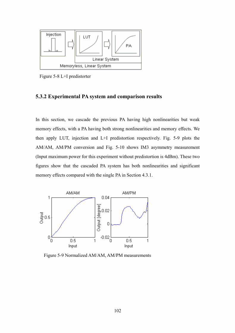
Figure 5-8 L+I predistorter
5.3.2 Experimental PA system and comparison results
In this section, we cascade the previous PA having high nonlinearities but weak
memory effects, with a PA having both strong nonlinearities and memory effects. We
then apply LUT, injection and L+I predistortion respectively. Fig. 5-9 plots the
AM/AM, AM/PM conversion and Fig. 5-10 shows IM3 asymmetry measurement
(Input maximum power for this experiment without predistortion is 4dBm). These two
figures show that the cascaded PA system has both nonlinearities and significant
memory effects compared with the single PA in Section 4.3.1.
Figure 5-9 Normalized AM/AM, AM/PM measurements
102

Figure 5-10 IM3 asymmetries at different two-tone input powers
Figure 5-11 Comparison of power spectra
103
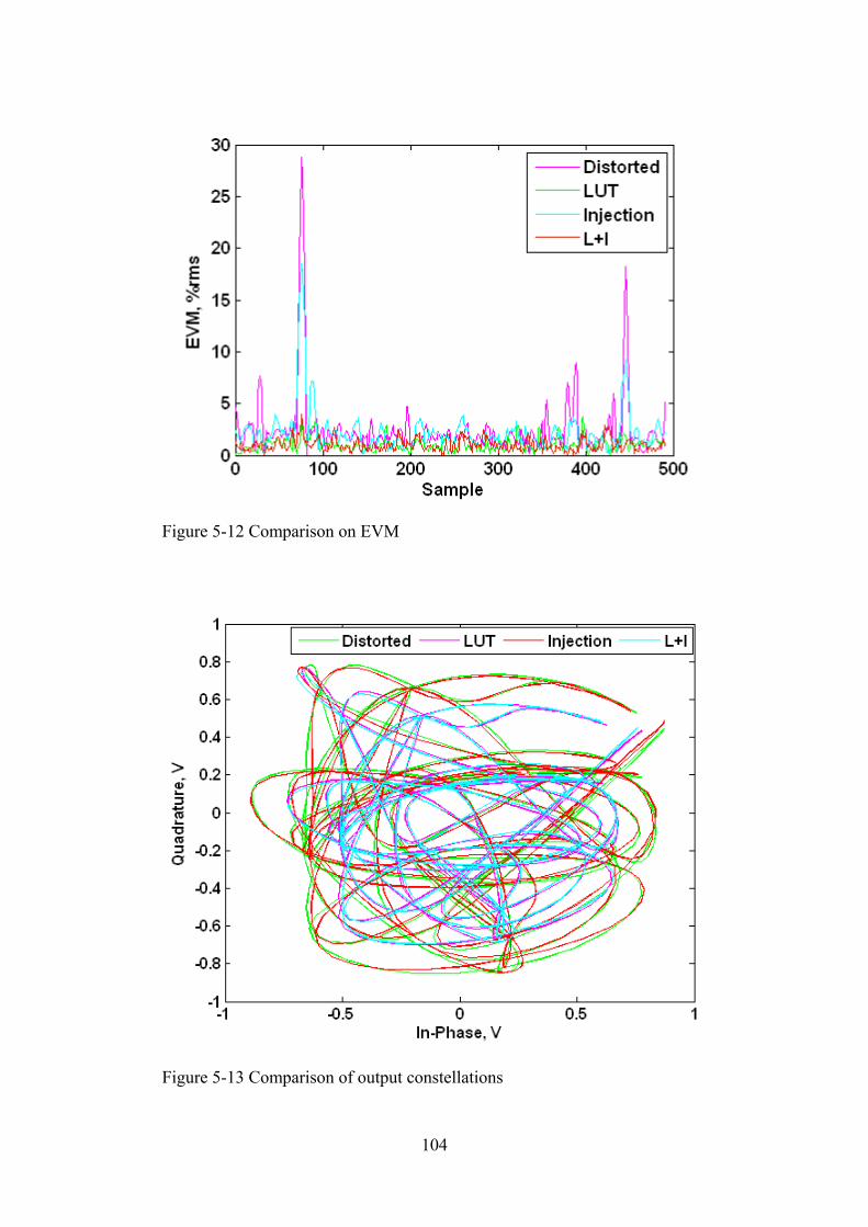
Figure 5-12 Comparison on EVM
Figure 5-13 Comparison of output constellations
104

TABLE 5-2 EXPERIMENTAL MEASUREMENTS
ACPR reduction
(dBc)
Average EVM
(%rms`)
Average output
magnitude (Volt)
Peak value (Volt)
Crest factor (input 2.075)
Distorted N/A 2.5330 0.6138 1.0147 1.6531 LUT 18 1.0399 0.4851 1.0143 2.0908
Injection 25 2.2688 0.5991 1.0277 1.7154 L+I 25 1.0041 0.4810 1.0119 2.1038
Fig. 5-11 shows the spectral regrowth, Fig. 5-12 shows the EVM and Fig. 5-13 shows
the output constellation for all original distorted signals, LUT, injection and L+I
predistortion. Table 5-2 lists the comparative results. As expected, L+I has a linear
gain back-off to compensate the compression, which is similar to LUT, and it can
address each sub-frequency to cancel the remaining memory effects, which is similar
to injection. As a result, it can improve EVM effectively and reduce spectral regrowth
down to the noise floor.
Another application of L+I is demonstrated in [63]. It is applied in a highly-efficient
broadband Inverse Class E PA. Improvement of approximately 40 dB for spectral
regrowth reduction (Fig. 5-14) and 0.7% EVM (rms) in a 16 QAM signal is achieved.
Compared with published memory polynomial models, L+I can reduce spectral
regrowth and improve EVM as well. The advantage of L+I is that, the LUT is
applicable to the nonlinearities while the injection is applicable to memory effects.
This L+I predistortion may be useful for further research, such as using predistortion
to separate nonlinearities and memory effects in a PA. In contrast, the coefficients in
memory polynomial models do not obviously separate or indicate the extent of the
nonlinearities and memory effects in PAs.
105

Figure 5-14 Application of L+I in an Inverse Class E PA
5.4 Summary
Although the injection technique in Chapter 4 was proven to work in the frequency
domain, it results in inevitably poor EVM, as demonstrated in Section 5.2. Therefore,
we propose a combined predistortion technique in this chapter, which applies both
LUT and injection. The idea is that it can use LUT to reduce most of the nonlinearities
and then apply injection to remove the residual spectral regrowth. This combined
predistortion technique has two advantages compared with the single injection. First,
it doesn’t need a matrix (in two-tone tests) nor iterations (in wideband signals) to
compensate the interactions. Secondly, it can reduce both ACPR and EVM, when the
PA has both strong nonlinearities and memory effects, as demonstrated in Section 5.3.
106

CHAPTER 6
SUMMARY AND CONCLUSION 6.1 Summary
Due to the growing number of mobile users and the trend towards multi-band and
multi-mode communication systems, high efficiency and high linearity power
amplifiers are more and more desirable. Therefore, a high efficiency power amplifier
with an integrated linearization technique is increasingly popular today. During the
PhD research, we have analyzed and implemented a range of published and novel
predistortion techniques. The range covers from memoryless AM/AM, AM/PM
conversion to memory Volterra, and finally our proposed combined LUT plus
injection. Meanwhile, the testing amplifiers varied from commercial memoryless
power amplifier, inverse class E power amplifier, to a cascaded power amplifier
system which contains both nonlinearities and memory effects.
This thesis began with a brief introduction of linearization techniques, and basic
models of both analogue and digital predistortion, in Chapter 1. We chose digital
predistortion as our main linearization technique, and begin to analyze numbers of
power amplifier models and the corresponding digital predistortion techniques in
Chapter 2.
In Chapter 2, we firstly discussed the power amplifiers models which are divided into
two categories. The first category is memoryless models, which includes AM/AM,
AM/PM conversion, memoryless polynomial, frequency-independent Saleh model.
The second category considers both nonlinearities and memory effects, which
contains a frequency-dependent nonlinear quadrature model, ARMA model, Volterra
107
model, memory polynomial model, Wiener model, and neural network model. Most
of their inverse models are also depicted later in the same chapter, which are AM/AM,
AM/PM conversion, inverse Volterra, inverse memory polynomial, Hammerstein, and
neural network model. All of the inverse models are implemented in the digital
predistorter. Further, we introduced digital injection predistortion. Unlike the
traditional digital predistortions which are inverse power amplifier models, this
injection technique generates phasors in anti-phase to those representing the
intermodulation products, in order to cancel each other at the output port. This is
attractive because it is good at dealing with memory effects in two-tone tests. Some
novel improvements for the injection are described in the following Chapter 3 and 4.
In Chapter 3, we proposed and demonstrated novel methods on measurement and
injection for intermodulation products in two-tone tests, which were subsequently
published in [8]. We brought several innovations to the published techniques. The new
measurement can clearly and easily describe the relationship between injected and
output intermodulation products. Based on this discovered relationship, either lower
or upper sideband IM3 injection can be calculated instead of manual tuning.
Interaction between lower and upper sideband IM3 products has been discovered for
the first time with this new measurement. To our knowledge, this interaction has not
been proposed or discussed in published papers before. As a result, further IM3
reductions have been achieved while considering these interactions. In order to
maximize its merit, we attempt to apply the same technique in wideband 16 QAM
signal in Chapter 4.
In Chapter 4, the same injection technique is applied to a 16 QAM signal. However,
the matrix approach proposed in Chapter 3 is no longer practical since what we reduce
are not lower and upper IM3 products, but the whole spectral regrowth. As we know,
the interaction is caused by the third order nonlinearities of the power amplifier while
the cancellation of spectral regrowth is through the linear gain of the power amplifier.
So the amplitudes of anti-phase phasors are bigger than those of the new interactions.
108
We can adjust the injection to become smaller in order to cancel part of the spectral
regrowth while generating negligible interactions, step by step in the whole injection.
Hence, an alternative iterative method is proposed to compensate interaction problems
in 16 QAM injections. Since our injection can effectively control each sub-frequency,
therefore, our results give much better spectral regrowth reduction compared with
published works. In the end of this chapter, we have completely demonstrated its
capacity for dealing with memory effects by showing that, as an extreme case, it can
be used to suppress only the upper sideband of spectral regrowth. Although injection
performs good spectral regrowth reduction even for power amplifiers that show
significant memory effects, it still has a few disadvantages which limit its applications.
Further discussions and a solution were presented in Chapter 5.
Communication signals not only require high spectrum efficiency, i.e. low frequency
interference, but also high accuracy. A widely accepted measure applicable to this is
the EVM in 16 QAM signal. In the published works on injection, authors typically
focus on intermodulation products reduction in spectrum rather than I-Q signal
precision. No relevant measurements such as EVM are given. Our measurement
shows that injection will result in poor EVM compared with traditional LUT
linearization. In Chapter 5, we firstly went back to a simple LUT using AM/AM and
AM/PM conversion. And then we compare LUT and injection, regarding to their
mathematical models, experimental results such as spectral regrowth reduction, output
power, signal crest factor and EVM. With these analyses, we finally propose a new
digital predistortion technique, which combine injection and LUT. The idea behind
this combination is to use LUT to reduce most of the nonlinearities first, and then
injection to reduce the rest of the spectral regrowth. This LUT plus injection
predistortion is applied to a cascaded power amplifier system which has shown both
significant nonlinearities and memory effects. With this predistortion method, both
spectral regrowth and EVM show an improvement when compared with any single
predistortion technique.
109

6.2 Major contributions and achievements
In the research, we have the following novel contribution on digital predistortion
linearization techniques:
a. Improvements on traditional digital injection in two-tone test. Firstly, we reveal the
phase relationships between the two main output tones and the output intermodulation
products. Measurements on IM3 including amplitude and phase are given. Secondly,
we proposed a new mathematical relationship on injected and output intermodulation
products. Hence, we are the first to identify these interactions in the injection method
and give solutions. With this improvement, the IM3 products have been further
reduced when the power amplifier is driven harder. In our research, a 60 dB reduction
on IM3 is achieved.
b. This new digital injection technique was firstly applied to 16 QAM wideband
signals. Because our novel injection technique can effectively control each
sub-frequency and consider interactions, it results a 30 dB reduction on spectral
regrowth, which is better than the published works. Further, we can manage to
reduce one sideband of spectral growth, leaving the other sideband. This can
demonstrate its capabilities of dealing with memory effects.
c. We have been the first authors to analyze injection with regard to EVM
measurements. We determined that injection does not improve the EVM. So we are
the first to combine LUT and injection for wideband signal predistortion. This new
L+I linearization can handle nonlinearities and memory effects, hence giving both
better EVM (0.7% rms) and ACPR improvements (40dB) than any single technique.
110

6.3 Suggestions for future work
The work can be implemented into a FPGA board or DSP board. When using
FPGA as a PD, the delay caused by the circuit or the processing can be
compensated by adding digital buffer inside the board. Choosing a suitable clock
signal is a key work. So far, we have implemented the LUT algorithm into FPGA
broad. However, the injection part which will include the convolution integrations
is under construction.
The experiment for injection in thesis is to correct a repeat signal, which is known
before the correction. While the signal is unknown in a practical way, the FPGA
board can apply pipeline to calculate the injection before sending the signal. To
make it simple, we can have three different phase injections (instead of 10 in
Chapter 4) to identify the circle (e.g. in Figure 4-8). For example, we can inject
the components with identical amplitude but phases of 0o, 120o and 240o. The
FPGA board can have three blocks to perform the injection in parallel. We
assume the first block is to injection 0o phase component, the second block is to
injection 120o phase component and the third block is to inject the 240o phase
component. At the same time, the FPGA can have a fourth block to perform the
calculation for the correct injection. We can chop the signal which is going to be
sent into parts with the same time length. It can be marked with ①, ②, ③, ④
and so on. The performance of the FPGA is listed in Table 6-1.
FPGA (block 1) ① ② ③ ④ ⑤ ……
FPGA (block 2) ① ② ③ ④ ⑤ ……
FPGA (block 3) ① ② ③ ④ ⑤ ……
FPGA (block 4) ① ② ③ ④
111

Timing T1 T2 T3 T4 T5 ……
Table 6-1 FPGA pipeline
The first line in Table 6-1 represents how block 1 inside the FPGA working in
different time period. For example, in the time period T1, it performs phase 0o
injection to signal ①; in the time period T2, it performs phase 0o injection to
signal ②, and so on. The second line in Table 6-1 represents how block 2 which
is 120o phase injection, working in different time period. It is similar to block 1.
The third line in Table 6-1 represents how block 3 which is 240o phase injection,
working in different time period. It is similar to block 1 as well. The fourth line in
Table 6-1 represents block 4 which is to calculate the correct injection, working in
different time period. In T1, because the circle of signal ① is not completed, so it
does not carry any performance. In T2, when the circle of signal ① is identified,
block 4 will calculate its center and radius and find out the correct inject
component for signal ①. In T3, block 4 will calculate the injection for signal ②,
and so on. So for any piece of the signal, it will take only two time period to find
out the correct injection, which means the delay for this injection is two time
period. This PGA parallel working system will shorten the injection measuring
time hence to mitigate the time delay issue, and make the injection more realistic.
The power consumption of the FPGA board plays an important roll for the
predistorter, because the original aim of predistortion is to improve the PA’s
linearity while maintaining its power efficiency. So far, the power consumption of
the FPGA board can be more than 1200 mW. This power level indicates that
predistorter using FPGA is not ideal for handsets, but it can be implemented into
base station.
The L+I predistortion has the potential to be controlled using artificial
intelligence techniques. The advantage is that the coefficients of injection and
112

LUT and can be calculated automatically rather than manual measurement and
calculation.
6.4 Conclusions
In this thesis, we have summarized different published power amplifier models and
their inverse models for predistortion. However, memory effects which affect these
digital predistortion motivated our further research on digital predistortion.
We have proposed our LUT plus injection predistortion. It has several advantages as
follows. Firstly, the injection results reported here are superior to those in previously
published works. Secondly it can deal with nonlinearities and memory effects when
compared with any single techniques. As a result, it gives much better EVM and
ACPR reduction, even when the operated power amplifier or cascaded power
amplifier system is driven harder resulting in bigger nonlinearities and memory
effects.
This new linearization technique can be further developed by using neural networks to
incorporate artificial intelligence capabilities and greater adaptivity. This technique
can be applied to using FPGA or DSP boards in the future to maximize its application.
113
References
[1] K. Y. Chan and A. Bateman, "Analytical and Measured Performance of the Combined Analog Locked Loop Universal Modulator (Callum)," Iee Proceedings-Communications, vol. 142, issue 5, pp. 297-306, Oct, 1995.
[2] P. B. Kenington, High-linearity RF Amplifier Design. 685 Canton Street, Norwood, MA Artech House, 2000.
[3] H. Jardon and H. Vazquez, "A novel representation of AM-PM conversion," Emc - a Global Concern: Ieee 1995 International Symposium on Electromagnetic Compatibility, Symposium Record, issue 401-405, 1995.
[4] R. Blum and M. C. Jeruchim, "Modeling nonlinear amplifiers for communication simulation," Communications, 1989. ICC 89, BOSTONICC/89. Conference record. World Prosperity Through Communications, IEEE International Conference, vol. 3, issue 1468-1472, June, 1989.
[5] N. B. Carvalho and J. C. Pedro, "Multi-tone intermodulation distortion performance of 3rd order microwave circuits," 1999 Ieee Mtt-S International Microwave Symposium Digest, Vols 1-4, issue 763-766, 1999.
[6] A. A. M. Saleh, "Frequency-Independent and Frequency-Dependent Non-Linear Models of Twt Amplifiers," IEEE Transactions on Communications, vol. 29, issue 11, pp. 1715-1720, 1981.
[7] J. H. K. Vuolevi, T. Rahkonen, and J. P. A. Manninen, "Measurement technique for characterizing memory effects in RF power amplifiers," IEEE Transactions on Microwave Theory and Techniques, vol. 49, issue 8, pp. 1383-1389, Aug, 2001.
[8] M. Xiao and P. Gardner, "Characterisation, analysis and injection of two-tone third-order intermodulation products in an amplifier," IET Microwaves, Antennas & Propagation, vol. 3, issue 3, pp. 443-455, 2009.
[9] W. Woo, M. D. Miller, and J. S. Kenney, "A hybrid digital/RF envelope predistortion linearization system for power amplifiers," IEEE Transactions on Microwave Theory and Techniques, vol. 53, issue 1, pp. 229-237, Jan, 2005.
[10] A. Richards, K. A. Morris, and J. P. McGeehan, "Removing the effects of baseband impedance on distortion in FET amplifiers," IET Proceedings-Microwaves Antennas and Propagation, vol. 153, issue 5, pp. 401-406, Oct, 2006.
[11] M. T. Abuelmaatti, "Frequency-Dependent Nonlinear Quadrature Model for Twt Amplifiers," IEEE Transactions on Communications, vol. 32, issue 8, pp. 982-986, 1984.
[12] C. J. Clark, G. Chrisikos, M. S. Muha, A. A. Moulthrop, and C. P. Silva,
114
"Time-domain envelope measurement technique with application to wideband power amplifier modeling," IEEE Transactions on Microwave Theory and Techniques, vol. 46, issue 12, pp. 2531-2540, Dec, 1998.
[13] C. Eun and E. J. Powers, "A new Volterra predistorter based on the indirect learning architecture," IEEE Transactions on Signal Processing, vol. 45, issue 1, pp. 223-227, Jan, 1997.
[14] R. Raich, H. Qian, and G. T. Zhou, "Orthogonal polynomials for power amplifier modeling and predistorter design," IEEE Transactions on Vehicular Technology, vol. 53, issue 5, pp. 1468-1479, Sep, 2004.
[15] H. C. Ku and J. S. Kenney, "Behavioral modeling of nonlinear RF power amplifiers considering memory effects," IEEE Transactions on Microwave Theory and Techniques, vol. 51, issue 12, pp. 2495-2504, Dec, 2003.
[16] D. R. Morgan, Z. X. Ma, J. Kim, M. G. Zierdt, and J. Pastalan, "A generalized memory polynomial model for digital predistortion of RF power amplifiers," IEEE Transactions on Signal Processing, vol. 54, issue 10, pp. 3852-3860, Oct, 2006.
[17] L. Ding, G. T. Zhou, D. R. Morgan, Z. X. Ma, J. S. Kenney, J. Kim, and C. R. Giardina, "A robust digital baseband predistorter constructed using memory polynomials," IEEE Transactions on Communications, vol. 52, issue 1, pp. 159-165, Jan, 2004.
[18] H. C. Ku, M. D. McKinley, and J. S. Kenney, "Quantifying memory effects in RF power amplifiers," IEEE Transactions on Microwave Theory and Techniques, vol. 50, issue 12, pp. 2843-2849, Dec, 2002.
[19] A. Ahmed, E. Srinidhi, and G. Kompa, "Efficient PA Modeling Using Neural Network and Measurement Setup for Memory Effect Characterization in the Power Device," Microwave Symposium Digest, 2005 IEEE MTT-S International, issue 473-476, June, 2005.
[20] J. Namiki, "An Automatically Controlled Predistorter for Multilevel Quadrature Amplitude-Modulation," IEEE Transactions on Communications, vol. 31, issue 5, pp. 707-712, 1983.
[21] W. Woo and J. S. Kenney, "A new envelope predistortion linearization architecture for handset power amplifiers," Radio and Wireless Conference, 2004 IEEE, issue 175-178, 19-22 Sept, 2004.
[22] S. Kusunoki, K. Yamamoto, T. Hatsugai, H. Nagaoka, K. Tagami, N. Tominaga, K. Osawa, K. Tanabe, S. Sakurai, and T. Iida, "Power-amplifier module with digital adaptive predistortion for cellular phones," IEEE Transactions on Microwave Theory and Techniques, vol. 50, issue 12, pp. 2979-2986, Dec, 2002.
[23] W. Woo and J. S. Kenney, "A predistortion linearization system for high power amplifiers with low frequency envelope memory effects," 2005 IEEE MTT-S Int. Microwave Symp. Dig., issue 4, June, 2005.
[24] S. P. Stapleton and F. C. Costescu, "An Adaptive Predistorter for a Power-Amplifier Based on Adjacent Channel Emissions," IEEE Transactions on Vehicular Technology, vol. 41, issue 1, pp. 49-56, Feb, 1992.
115
[25] S. P. Stapleton, G. S. Kandola, and J. K. Cavers, "Simulation and Analysis of an Adaptive Predistorter Utilizing a Complex Spectral Convolution," IEEE Transactions on Vehicular Technology, vol. 41, issue 4, pp. 387-394, Nov, 1992.
[26] L. Ding, R. Raich, and G. T. Zhou, "A Hammerstein predistortion linearization design based on the indirect learning architecture," Acoustics, Speech, and Signal Processing, 2002. Proceedings. (ICASSP '02). IEEE International Conference on, vol. 3, issue 2689-2692, 13-17 May, 2002.
[27] T. J. Liu, S. Boumaiza, and F. M. Ghannouchi, "Augmented Hammerstein predistorter for linearization of broad-band wireless transmitters," IEEE Transactions on Microwave Theory and Techniques, vol. 54, issue 4, pp. 1340-1349, Apr, 2006.
[28] J. Kim and K. Konstantinou, "Digital predistortion of wideband signals based on power amplifier model with memory," Electronics Letters, vol. 37, issue 23, pp. 1417-1418, Nov 8, 2001.
[29] R. Sperlich, J. A. Sills, and J. S. Kenney, "Closed-loop digital pre-distortion with memory effects using genetic algorithms," Microwave Symposium Digest, 2005 IEEE MTT-S International, issue 4, June, 2005.
[30] D. Psaltis, A. Sideris, and A. A. Yamamura, "A multilayered neural network controller," IEEE JNL, vol. 8, issue 2, pp. 17 - 21, April, 1988.
[31] H. Qian and G. T. Zhou, "A neural network predistorter for nonlinear power amplifiers with memory," Digital Signal Processing Workshop, 2002 and the 2nd Signal Processing Education Workshop. Proceedings of 2002 IEEE 10th, issue 312-316, 13-16 Oct, 2002.
[32] K. C. Lee and P. Gardner, "Adaptive neuro-fuzzy inference system (ANFIS) digital predistorter for RF power amplifier linearization," IEEE Transactions on Vehicular Technology, vol. 55, issue 1, pp. 43-51, Jan, 2006.
[33] H. M. Deng, S. B. He, and J. B. Yu, "An adaptive predistorter using modified neural networks combined with a fuzzy controller for nonlinear power amplifiers," International Journal of Rf and Microwave Computer-Aided Engineering, vol. 14, issue 1, pp. 15-20, Jan, 2004.
[34] K. Krishnakumar, "Backpropagation Algorithm for a Generalized Neural Network Structure," Proceedings: Ieee Southeastcon 92, Vols 1 and 2, issue 646-649, 1992.
[35] T. Nitta, "An extension of the back-propagation algorithm to complex numbers," Neural Networks, vol. 10, issue 8, pp. 1391-1415, Nov, 1997.
[36] "Foundations of Fuzzy Logic," in Matlab help files. [37] J. S. R. Jang and C. T. Sun, "Neuro-Fuzzy Modeling and Control,"
Proceedings of the IEEE, vol. 83, issue 3, pp. 378-406, Mar, 1995. [38] J. S. R. Jang, "Anfis - Adaptive-Network-Based Fuzzy Inference System,"
IEEE Transactions on Systems Man and Cybernetics, vol. 23, issue 3, pp. 665-685, May-Jun, 1993.
[39] D. Rabijns, W. Van Moer, and G. Vandersteen, "Spectrally pure excitation signals: Only a dream?" IEEE Transactions on Instrumentation and
116
Measurement, vol. 53, issue 5, pp. 1433-1440, Oct, 2004. [40] K. J. Cho, D. H. Jang, S. H. Kim, J. Y. Kim, J. H. Kim, and S. P. Stapleton,
"An analog compensation method for asymmetric IMD characteristics of power amplifier," IEEE Microwave and Wireless Components Letters, vol. 14, issue 4, pp. 153-155, Apr, 2004.
[41] C. Crespo-Cadenas, J. Reina-Tosina, and M. J. Madero-Ayora, "Phase characterization of two-tone intermodulation distortion," 2005 IEEE MTT-S Int. Microwave Symp. Dig., Long Beach, CA, pp.1505-1508, June 2005
[42] C. Crespo-Cadenas, J. Reina-Tosina, and M. J. Madero-Ayora, "IM3 and IM5 phase characterization and analysis based on a simplified newton approach," IEEE Transactions on Microwave Theory and Techniques, vol. 54, issue 1, pp. 321-328, Jan, 2006.
[43] F. Ali, M. R. Moazzam, and C. Aitchison, "IMD elimination and CPR improvement for an 800 MHz HBT MMIC power amplifier," Radio Frequency Integrated Circuits (RFIC) Symposium, IEEE, Baltimore,MD, pp.69 - 71, June 1998
[44] A. Singh, J. E. Scharer, J. H. Booske, and J. G. Wohlbier, "Second- and third-order signal predistortion for nonlinear distortion suppression in a TWT," IEEE Transactions on Electron Devices, vol. 52, issue 5, pp. 709-717, May, 2005.
[45] M.Modeste, D.Budimir, M.R.Moazzam, and C.S.Aitchison, "Analysis and practical performance of a difference frequency technique for improving the multicarrier IMD performance of RF amplifiers," Technologies for Wireless Applications, 1999. Digest. 1999 IEEE MTT-S Symposium, Vancouver,BC,Canada, pp.53 - 56, Feb. 1999
[46] C. S. Leung and K. K. M. Cheng, "A new approach to amplifier linearization by the generalized baseband signal injection method," IEEE Microwave and Wireless Components Letters, vol. 12, issue 9, pp. 336-338, Sep, 2002.
[47] C. W. Fan and K. K. M. Cheng, "Theoretical and experimental study of amplifier linearization based on harmonic and baseband signal injection technique," IEEE Transactions on Microwave Theory and Techniques, vol. 50, issue 7, pp. 1801-1806, Jul, 2002.
[48] C. S. Aitchison, M. Mbabele, M. R. Moazzam, D. Budimir, and F. Ali, "Improvement of third-order intermodulation product of RF and microwave amplifiers by injection," IEEE Transactions on Microwave Theory and Techniques, vol. 49, issue 6, pp. 1148-1154, Jun, 2001.
[49] X. Q. Li, F. Han, T. M. Lok, M. R. Lyu, and G. B. Huang, "Improvements to the conventional layer-by-layer BP algorithm," Advances in Intelligent Computing, Pt 2, Proceedings, vol. 3645, issue 189-198, 2005.
[50] M. Wirth, A. Singh, J. Scharer, and J. Booske, "Third-order intermodulation reduction by harmonic injection in a TWT amplifier," IEEE Transactions on Electron Devices, vol. 49, issue 6, pp. 1082-1084, Jun, 2002.
[51] N. Mizusawa and S. Kusunoki, "Third- and fifth-order baseband component injection for linearization of the power amplifier in a cellular phone," IEEE
117
Transactions on Microwave Theory and Techniques, vol. 53, issue 11, pp. 3327-3334, Nov, 2005.
[52] K. A. Remley, D. E. Williams, D. M. M. P. Schreurs, and J. Wood, "Simplifying and, interpreting two-tone measurements," IEEE Transactions on Microwave Theory and Techniques, vol. 52, issue 11, pp. 2576-2584, Nov, 2004.
[53] A. Richards, K. A. Morris, and J. P. McGeehan, "Cancellation of electrical memory effects in FET power amplifiers," Microwave Conference, 2005 European, vol. 2, issue, 4-6 Oct, 2005.
[54] J. S. Kenney and P. Fedorenko, "Identification of RF Power Amplifier Memory Effect Origins using Third-Order Intermodulation Distortion Amplitude and Phase Asymmetry," Microwave Symposium Digest, 2006. IEEE MTT-S International, issue 1121 - 1124, 11-16 June, 2006.
[55] A. Walker, M. Steer, and K. G. Gard, "A vector intermodulation analyzer applied to behavioral modeling of nonlinear amplifiers with memory," IEEE Transactions on Microwave Theory and Techniques, vol. 54, issue 5, pp. 1991-1999, May, 2006.
[56] J. P. Martins and N. B. Carvalho, "Spectral filtering setup for uncorrelated multi-tone phase and amplitude measurement," 34Th European Microwave Conference, Vols 1-3, Conference Proceedings, issue 201-204, 2004.
[57] J. P. Martins and N. B. Carvalho, "Multitone phase and.amplitude measurement for nonlinear device characterization," Ieee Transactions on Microwave Theory and Techniques, vol. 53, issue 6, pp. 1982-1989, Jun, 2005.
[58] J. P. Martins, N. B. Carvalho, and J. C. Pedro, "Practical multitone amplitude and phase characterization," 2005 Asia-Pacific Microwave Conference Proceedings, Vols 1-5, issue 3055-3058, 2005.
[59] J. C. Pedro and J. P. Martins, "Amplitude and phase characterization of nonlinear mixing products," IEEE Transactions on Microwave Theory and Techniques, vol. 54, issue 8, pp. 3237-3245, Aug, 2006.
[60] S. Y. Lee, Y. S. Lee, and Y. H. Jeong, "A novel phase measurement technique for IM3 components in RF power amplifiers," IEEE Transactions on Microwave Theory and Techniques, vol. 54, issue 1, pp. 451-457, Jan, 2006.
[61] D. Budimir, N. Males-Ilic, B. Milovanovic, and M. Tomic, "Linearization of multichannel amplifiers with the injection of second harmonics into the amplifier and predistortion circuit," 6th International Conference on Telecommunications in Modern Satellite, Cable and Broadcasting Service, 2003., vol. 1, issue 214-217, 1-3 Oct, 2003.
[62] J. Yi, Y. Yang, M. Park, W. Kang, and B. Kim, "Analog predistortion linearizer for high-power RF amplifiers," IEEE Transactions on Microwave Theory and Techniques, vol. 48, issue 12, pp. 2709-2713, Dec, 2000.
[63] M. Thian, M. Xiao, and P. Gardner, "Digital Baseband Predistortion Based Linearized Broadband Inverse Class-E Power Amplifier," IEEE Transactions on Microwave Theory and Techniques, vol. 57, issue 2, pp. 323 - 328, Feb, 2009.
118

APPENDIX A
The information of power amplifiers ZHL-4240 can be found in the website:
http://www.minicircuits.com/pdfs/ZHL-4240.pdf
119

APPENDIX B
The information of I/Q Modulation Generator R&S® AMIQ can be found in the
website: http://www2.rohde-schwarz.com/product/AMIQ.html
120

Appendix C
The information of Signal Generator Family R&S SMIQ can be found in the website:
http://www2.rohde-schwarz.com/product/smiq.html
121

Appendix D
The program below is written in C++ Builder, for the purpose of connecting PC with modulator (AMIQ). The AMIQ has a 14-bit DAC output, which means the normalized voltage can vary from 0 to 1, with the interval of 2-14. As a result, the ratio between the maximum power to the minimum power is 214*2, which is nearly 84 dBc. All the programs in the appendix are created by the author. #include <vcl.h> #include <stdio.h> #include <math.h> #pragma hdrstop #include "P_port.h" //--------------------------------------------------------------------------- #pragma package(smart_init) #pragma link "MSCommLib_OCX" #pragma resource "*.dfm" TForm1 *Form1; //--------------------------------------------------------------------------- __fastcall TForm1::TForm1(TComponent* Owner) : TForm(Owner) { } //--------------------------------------------------------------------------- void __fastcall TForm1::FormCreate(TObject *Sender) //define the user interface at the beginning of program { auto_i=0; auto_j=0; auto_k=0; if (MSComm->PortOpen==true) MSComm->PortOpen=false; Button_Con->Enabled=true; Button_DisCon->Enabled=false; Shape->Shape=stCircle; Shape->Brush->Color=clRed;
122

All_InVisible(); Connection->TabVisible=false; ComboBox_Fre->Text="MHz"; ComboBox_Amp->Text="I:"; ComboBox_RamQuery->Text="File Name"; Edit_C2->Visible=false; Edit_C3->Visible=false; Edit_C4->Visible=false; Label_C2->Visible=false; Label_C3->Visible=false; Label_C4->Visible=false; Label_CF2->Visible=false; Label_CF3->Visible=false; Label_CF4->Visible=false; Edit_CF2->Visible=false; Edit_CF3->Visible=false; Edit_CF4->Visible=false; ComboBox_CF2->Visible=false; ComboBox_CF3->Visible=false; ComboBox_CF4->Visible=false; Label_IData->Visible=false; Label_QData->Visible=false; Edit_IData->Visible=false; Edit_QData->Visible=false; Edit_DataFile->Visible=true; RadioGroup_IQ->ItemIndex=0; ProgressBar_SG->Position=0; } //--------------------------------------------------------------------------- void __fastcall TForm1::Button_ConClick(TObject *Sender) //botton for connection { if(MSComm->PortOpen!=true&&ComboBox->Text!="Connection Config") { //define port if (ComboBox->Text=="Com1") MSComm->CommPort=1; else MSComm->CommPort=2; //set protocol MSComm->Settings="9600,n,8,1"; MSComm->InputMode=0;
123

MSComm->Handshaking=2; MSComm->SThreshold=1; MSComm->RThreshold=1; MSComm->PortOpen=true; //program interface config Button_Con->Enabled=false; Button_DisCon->Enabled=true; Shape->Brush->Color=clGreen; All_Visible(); } else if (ComboBox->Text=="Connection Config") Application->MessageBox("Port not selected.","Error Message",MB_OK); } //--------------------------------------------------------------------------- void __fastcall TForm1::Button_DisConClick(TObject *Sender) //click for disconnect { //disconnection MSComm->PortOpen=false; //program interface config Button_Con->Enabled=true; Button_DisCon->Enabled=false; Shape->Brush->Color=clRed; All_InVisible(); } //--------------------------------------------------------------------------- void __fastcall TForm1::Button_SendClick(TObject *Sender) //botton for send command { if (!MSComm->PortOpen) Application->MessageBox("Port not open.","Error Message",MB_OK); else Transmit(); } //--------------------------------------------------------------------------- void __fastcall TForm1::Transmit() //function for transmit text in "connection page" { if (!MSComm->PortOpen)
124

Application->MessageBox("Port not open.","Error Message",MB_OK); else { MSComm->Output=StringToOleStr(Edit->Text+"\n"); Edit->Text="T: "+Edit->Text; Memo1->Lines->Add(Edit->Text); Edit->Text=""; } } //----------------------------------------------- void __fastcall TForm1::All_Visible() //all pages visible { Property->TabVisible=true; Signal_Gen->TabVisible=true; } //----------------------------------------------- void __fastcall TForm1::All_InVisible() //all pages invisible { Property->TabVisible=false; Signal_Gen->TabVisible=false; } //--------------------------------------------- void __fastcall TForm1::EditKeyPress(TObject *Sender, char &Key) //if "enter" then transmit--in "connection page" { if (Key==13) Transmit(); } //--------------------------------------------------------------------------- void __fastcall TForm1::MSCommComm(TObject *Sender) //if received any char in serial port { AnsiString str; OleVariant s; if(MSComm->CommEvent==comEvReceive) { //if buffer got data
125

while (MSComm->InBufferCount) { //receive data s=MSComm->Input; //change to AnsiString data str=str+s.AsType(varString); for (int i=0;i<90999999;i++); } if (PageControl->ActivePageIndex==0) // if the buff receive Rthreshold number of data //display data into memo Memo1->Lines->Add("R: "+str); else if (PageControl->ActivePageIndex==1) Memo2->Lines->Add(str); } } //--------------------------------------------------------------------------- Appendix A C++builder graphic user interface program for connecting PC with modulator AMIQ (designed by the author) void __fastcall TForm1::ClearClick(TObject *Sender) //pop up menu for memo in "connection page" { if (PageControl->ActivePageIndex==0) Memo1->Text=""; else if (PageControl->ActivePageIndex==1) Memo2->Text=""; } //--------------------------------------------------------------------------- void __fastcall TForm1::Button_RSTClick(TObject *Sender) //command of reset { MSComm->Output=StringToOleStr("*RST\n"); } //--------------------------------------------------------------------------- void __fastcall TForm1::Button_idnClick(TObject *Sender) //command of identification { MSComm->Output=StringToOleStr("*IDN?\n");
126

} //--------------------------------------------------------------------------- void __fastcall TForm1::Botton_SineClick(TObject *Sender) //command of sending sine wave { MSComm->Output=StringToOleStr("MMEM:LOAD RAM,'SINE.WV'\nARM\nTRIG\noutput:i fix\noutput:q fix\n"); } //--------------------------------------------------------------------------- void __fastcall TForm1::Edit_ampKeyPress(TObject *Sender, char &Key) //command of changing amplitude { if (Key==13) { if (ComboBox_Amp->Text=="I:") MSComm->Output=StringToOleStr("OUTP:I:AMPL "+Edit_amp->Text+"v\nOUTP:I var\n"); else if (ComboBox_Amp->Text=="Q:") MSComm->Output=StringToOleStr("OUTP:Q:AMPL "+Edit_amp->Text+"v\nOUTP:Q var\n"); } } //--------------------------------------------------------------------------- void __fastcall TForm1::Edit_clocKeyPress(TObject *Sender, char &Key) //command of changing clock { if (Key==13) { MSComm->Output=StringToOleStr("CLOC "+Edit_cloc->Text+ComboBox_Fre->Text+"\n"); } } //--------------------------------------------------------------------------- void __fastcall TForm1::Button_clocClick(TObject *Sender) //command of asking clock { MSComm->Output=StringToOleStr("SOUR:CLOCK?\n"); } //---------------------------------------------------------------------------
127

void __fastcall TForm1::Button_AmpClick(TObject *Sender) //command of asking amplitude { MSComm->Output=StringToOleStr("OUTP:"+ComboBox_Amp->Text+"AMPL?\n"); } //--------------------------------------------------------------------------- void __fastcall TForm1::Button_RamQueryClick(TObject *Sender) //command of asking tag { if (ComboBox_RamQuery->Text=="File Name") MSComm->Output=StringToOleStr("MEM:NAME?\n"); else if (ComboBox_RamQuery->Text=="All Tag") MSComm->Output=StringToOleStr("MEM:DATA?\n"); else MSComm->Output=StringToOleStr("MEM:DATA? RAM,'"+ComboBox_RamQuery->Text+"'\n"); } //--------------------------------------------------------------------------- void __fastcall TForm1::Button_DualClick(TObject *Sender) //command of sending dultone waveform { MSComm->Output=StringToOleStr("MMEM:LOAD RAM,'dualtone.WV'\nARM\nTRIG\noutput:i fix\noutput:q fix\n"); } //--------------------------------------------------------------------------- void __fastcall TForm1::Button_FilClick(TObject *Sender) //command of sending filter { MSComm->Output=StringToOleStr("OUTP:"+ComboBox_FIL_Ch->Text+"filt "+ComboBox_FIL->Text+"\n"); } //--------------------------------------------------------------------------- void __fastcall TForm1::Button_filterClick(TObject *Sender) //command of asking filter { MSComm->Output=StringToOleStr("OUTP:"+ComboBox_FIL_Ch->Text+"filt?\n");
128

} //--------------------------------------------------------------------------- void __fastcall TForm1::Button_mineClick(TObject *Sender) //command of sending self generate waveform { Sig_Gen(); } //------------------------------------------------------------------------- void __fastcall TForm1::Sig_Gen() { ProgressBar_SG->Position=0; unsigned short Data[60000]; float data_float; int i,num; AnsiString num1,num2; FILE *fp,*fp1,*fp2; OleVariant Txbuff; if (RadioGroup_IQ->ItemIndex==0) //reading combine data { fp=fopen(Edit_DataFile->Text.c_str(),"rt"); num=0; //reading data while (1) { if (fscanf(fp,"%f",&data_float)==EOF) break; Data[num]=(unsigned short)(32768.0+(data_float*32000.0)+0.5); Data[num]&=0xFFFC; num++; } num--; fclose(fp); } else //reading IQ signal respectivly { fp1=fopen(Edit_IData->Text.c_str(),"rt"); fp2=fopen(Edit_QData->Text.c_str(),"rt"); num=0; //reading data
129
while (1) { if (fscanf(fp1,"%f",&data_float)==EOF) break; Data[num]=(unsigned short)(32768.0+(data_float*32000.0)+0.5); Data[num]&=0xFFFC; num++; if (fscanf(fp2,"%f",&data_float)==EOF) break; Data[num]=(unsigned short)(32768.0+(data_float*32000.0)+0.5); Data[num]&=0xFFFC; num++; } num--; fclose(fp1); fclose(fp2); } ProgressBar_SG->Position=2; if (num%2==0) num--; //send file info num2=AnsiString((num+1)*2+3); num1=AnsiString(23+num2.Length()+(num+1)*2+6); MSComm->Output=StringToOleStr("*RST\n"); MSComm->Output=StringToOleStr("mmem:data 'mycur.wv', #"+AnsiString(num1.Length())+num1+"{TYPE: WV, 0}{WAVEFORM-"+num2+": 0,#"); MSComm->PortOpen=false; MSComm->InputMode=1; MSComm->PortOpen=true; ProgressBar_SG->Position=5; //send bitstream for (i=0;i<=num;i++) { Txbuff=VarArrayCreate(OPENARRAY(int,(0,1)),varByte); Txbuff.PutElement((unsigned char)Data[i],0); Txbuff.PutElement((unsigned char)(Data[i]/256),1); MSComm->Output=Txbuff; ProgressBar_SG->Position=5+(int)(i*94/num); } MSComm->PortOpen=false; MSComm->InputMode=0;
130

MSComm->PortOpen=true; MSComm->Output=StringToOleStr("}\n"); //load waveform ProgressBar_SG->Position=100; MSComm->Output=StringToOleStr("MMEM:LOAD RAM,'mycur.WV'\nARM\nTRIG\noutput:i fix\noutput:q fix\n"); } //--------------------------------------------------------------------------- void __fastcall TForm1::ComboBox_Num_BChange(TObject *Sender) //command of changing number of carrier { if (ComboBox_Num_B->ItemIndex==0) { Edit_C2->Visible=false; Edit_C3->Visible=false; Edit_C4->Visible=false; Label_C2->Visible=false; Label_C3->Visible=false; Label_C4->Visible=false; Label_CF2->Visible=false; Label_CF3->Visible=false; Label_CF4->Visible=false; Edit_CF2->Visible=false; Edit_CF3->Visible=false; Edit_CF4->Visible=false; ComboBox_CF2->Visible=false; ComboBox_CF3->Visible=false; ComboBox_CF4->Visible=false; } else if (ComboBox_Num_B->ItemIndex==1) { Edit_C2->Visible=true; Edit_C3->Visible=false; Edit_C4->Visible=false; Label_C2->Visible=true; Label_C3->Visible=false; Label_C4->Visible=false; Label_CF2->Visible=true; Label_CF3->Visible=false; Label_CF4->Visible=false; Edit_CF2->Visible=true; Edit_CF3->Visible=false; Edit_CF4->Visible=false;
131

ComboBox_CF2->Visible=true; ComboBox_CF3->Visible=false; ComboBox_CF4->Visible=false; } else if (ComboBox_Num_B->ItemIndex==2) { Edit_C2->Visible=true; Edit_C3->Visible=true; Edit_C4->Visible=false; Label_C2->Visible=true; Label_C3->Visible=true; Label_C4->Visible=false; Label_CF2->Visible=true; Label_CF3->Visible=true; Label_CF4->Visible=false; Edit_CF2->Visible=true; Edit_CF3->Visible=true; Edit_CF4->Visible=false; ComboBox_CF2->Visible=true; ComboBox_CF3->Visible=true; ComboBox_CF4->Visible=false; } else if (ComboBox_Num_B->ItemIndex==3) { Edit_C2->Visible=true; Edit_C3->Visible=true; Edit_C4->Visible=true; Label_C2->Visible=true; Label_C3->Visible=true; Label_C4->Visible=true; Label_CF2->Visible=true; Label_CF3->Visible=true; Label_CF4->Visible=true; Edit_CF2->Visible=true; Edit_CF3->Visible=true; Edit_CF4->Visible=true; ComboBox_CF2->Visible=true; ComboBox_CF3->Visible=true; ComboBox_CF4->Visible=true; } } //---------------------------------------------------------------------------
132

void __fastcall TForm1::RadioGroup_IQClick(TObject *Sender) { //changing data source of self generation if (RadioGroup_IQ->ItemIndex==0) { Label_IData->Visible=false; Label_QData->Visible=false; Edit_IData->Visible=false; Edit_QData->Visible=false; Edit_DataFile->Visible=true; } else { Label_IData->Visible=true; Label_QData->Visible=true; Edit_IData->Visible=true; Edit_QData->Visible=true; Edit_DataFile->Visible=false; } } //--------------------------------------------------------------------------- void __fastcall TForm1::Button_BALQueryClick(TObject *Sender) //Balance query { MSComm->Output=StringToOleStr("outp:type?\n"); } //--------------------------------------------------------------------------- void __fastcall TForm1::Button_Bal_SendClick(TObject *Sender) //Balance define { if (ComboBox_BAL->ItemIndex==0) MSComm->Output=StringToOleStr("outp:type bal\n"); else MSComm->Output=StringToOleStr("outp:type UNB\n"); } //--------------------------------------------------------------------------- void __fastcall TForm1::Button_BAL_AMPClick(TObject *Sender) //Balance amplitude query {
133

if (ComboBox_BAL_IQ->ItemIndex==0) MSComm->Output=StringToOleStr("outp:i:ampl:bal?\n"); else MSComm->Output=StringToOleStr("outp:q:ampl:bal?\n"); } //--------------------------------------------------------------------------- void __fastcall TForm1::Edit_BALKeyPress(TObject *Sender, char &Key) //balance amplitude define { if (Key==13) { if (ComboBox_BAL_IQ->ItemIndex==0) MSComm->Output=StringToOleStr("outp:i var\noutp:i:ampl:bal "+Edit_BAL->Text+"V\n"); else MSComm->Output=StringToOleStr("outp:q var\noutp:q:ampl:bal "+Edit_BAL->Text+"V\n"); } } //--------------------------------------------------------------------------- void __fastcall TForm1::Edit_passwordKeyPress(TObject *Sender, char &Key) //identification { if (Key==13&&Edit_password->Text=="AABBCC") { Connection->TabVisible=true; Edit_password->Text=""; Password->TabVisible=false; } } //--------------------------------------------------------------------------- void __fastcall TForm1::BitBtn_AutoClick(TObject *Sender) { RadioGroup_IQ->ItemIndex=1; Label_IData->Visible=true; Label_QData->Visible=true; Edit_IData->Visible=true; Edit_QData->Visible=true; Edit_DataFile->Visible=false; Edit_IData->Text="I"+AnsiString(auto_j)+AnsiString(auto_k)+".txt";
134

Edit_QData->Text="Q"+AnsiString(auto_j)+AnsiString(auto_k)+".txt"; auto_k++; if (auto_k==10) { auto_k=0; auto_j++; if (auto_j==10) { auto_j=0; auto_i++; } } Sig_Gen(); MSComm->Output=StringToOleStr("CLOC 100mhz\noutp:type bal\n"); } //--------------------------------------------------------------------------- void __fastcall TForm1::Button_SetIJKClick(TObject *Sender) { auto_i=ComboBox_I->ItemIndex; auto_j=ComboBox_J->ItemIndex; auto_k=ComboBox_K->ItemIndex; } //---------------------------------------------------------------------------
135
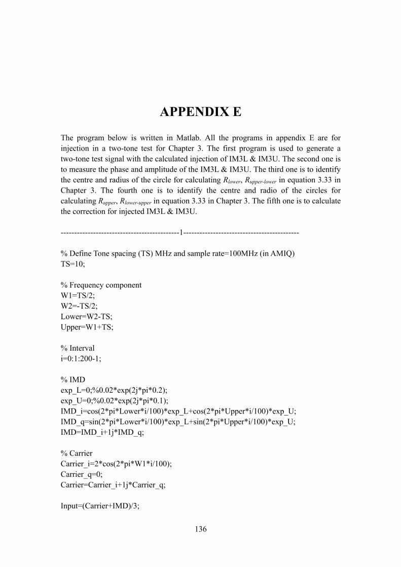
APPENDIX E The program below is written in Matlab. All the programs in appendix E are for injection in a two-tone test for Chapter 3. The first program is used to generate a two-tone test signal with the calculated injection of IM3L & IM3U. The second one is to measure the phase and amplitude of the IM3L & IM3U. The third one is to identify the centre and radius of the circle for calculating Rlower, Rupper-lower in equation 3.33 in Chapter 3. The fourth one is to identify the centre and radio of the circles for calculating Rupper, Rlower-upper in equation 3.33 in Chapter 3. The fifth one is to calculate the correction for injected IM3L & IM3U. --------------------------------------------1------------------------------------------- % Define Tone spacing (TS) MHz and sample rate=100MHz (in AMIQ) TS=10; % Frequency component W1=TS/2; W2=-TS/2; Lower=W2-TS; Upper=W1+TS; % Interval i=0:1:200-1; % IMD exp_L=0;%0.02*exp(2j*pi*0.2); exp_U=0;%0.02*exp(2j*pi*0.1); IMD_i=cos(2*pi*Lower*i/100)*exp_L+cos(2*pi*Upper*i/100)*exp_U; IMD_q=sin(2*pi*Lower*i/100)*exp_L+sin(2*pi*Upper*i/100)*exp_U; IMD=IMD_i+1j*IMD_q; % Carrier Carrier_i=2*cos(2*pi*W1*i/100); Carrier_q=0; Carrier=Carrier_i+1j*Carrier_q; Input=(Carrier+IMD)/3;
136
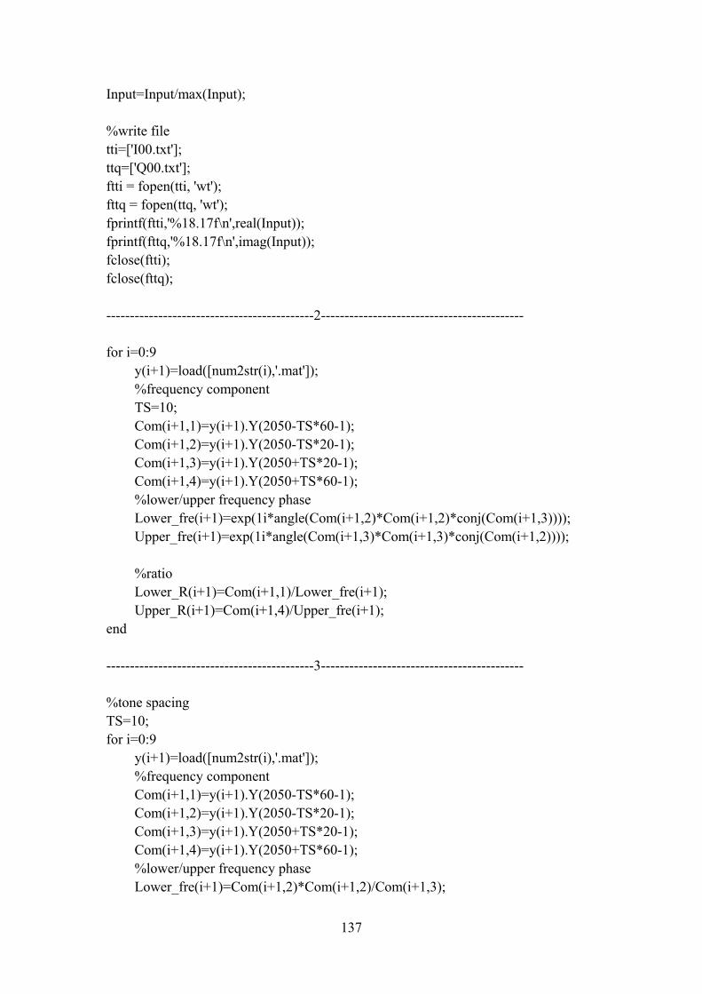
Input=Input/max(Input); %write file tti=['I00.txt']; ttq=['Q00.txt']; ftti = fopen(tti, 'wt'); fttq = fopen(ttq, 'wt'); fprintf(ftti,'%18.17f\n',real(Input)); fprintf(fttq,'%18.17f\n',imag(Input)); fclose(ftti); fclose(fttq); --------------------------------------------2------------------------------------------- for i=0:9 y(i+1)=load([num2str(i),'.mat']); %frequency component TS=10; Com(i+1,1)=y(i+1).Y(2050-TS*60-1); Com(i+1,2)=y(i+1).Y(2050-TS*20-1); Com(i+1,3)=y(i+1).Y(2050+TS*20-1); Com(i+1,4)=y(i+1).Y(2050+TS*60-1); %lower/upper frequency phase Lower_fre(i+1)=exp(1i*angle(Com(i+1,2)*Com(i+1,2)*conj(Com(i+1,3)))); Upper_fre(i+1)=exp(1i*angle(Com(i+1,3)*Com(i+1,3)*conj(Com(i+1,2)))); %ratio Lower_R(i+1)=Com(i+1,1)/Lower_fre(i+1); Upper_R(i+1)=Com(i+1,4)/Upper_fre(i+1); end --------------------------------------------3------------------------------------------- %tone spacing TS=10; for i=0:9 y(i+1)=load([num2str(i),'.mat']); %frequency component Com(i+1,1)=y(i+1).Y(2050-TS*60-1); Com(i+1,2)=y(i+1).Y(2050-TS*20-1); Com(i+1,3)=y(i+1).Y(2050+TS*20-1); Com(i+1,4)=y(i+1).Y(2050+TS*60-1); %lower/upper frequency phase Lower_fre(i+1)=Com(i+1,2)*Com(i+1,2)/Com(i+1,3);
137

Upper_fre(i+1)=Com(i+1,3)*Com(i+1,3)/Com(i+1,2); %ratio Lower_R(i+1)=Com(i+1,1)/(Lower_fre(i+1)/abs(Lower_fre(i+1))); Upper_R(i+1)=Com(i+1,4)/(Upper_fre(i+1)/abs(Upper_fre(i+1))); End %finding circle %left 3rd order x=0; Num_Cir=0; for i=1:8 for j=i+1:9 for k=j+1:10 a=2*(real(Lower_R(j))-real(Lower_R(i))); b=2*(imag(Lower_R(j))-imag(Lower_R(i))); c=(real(Lower_R(j)))^2+(imag(Lower_R(j)))^2-(real(Lower_R(i)))^2-(imag(Lower_R(i)))^2; d=2*(real(Lower_R(k))-real(Lower_R(j))); e=2*(imag(Lower_R(k))-imag(Lower_R(j))); f=(real(Lower_R(k)))^2+(imag(Lower_R(k)))^2-(real(Lower_R(j)))^2-(imag(Lower_R(j)))^2; Num_Cir=Num_Cir+1; x(Num_Cir)=(b*f-e*c)/(b*d-e*a)+1i*(d*c-a*f)/(b*d-e*a); end end end %refind center meanx=mean(x); covx=cov(x)^0.5; i=1; j=0; xx=0; while (i<=Num_Cir) if abs(x(i)-meanx)<covx; j=j+1; xx(j)=x(i); end i=i+1; end Center_left=mean(xx); Gain_need_left=abs(Center_left)/mean(abs(Lower_R(:)-Center_left));
138

i=1; while (angle((-Center_left)/(Lower_R(i)-Center_left))<0)||(angle((-Center_left)/(Lower_R(mod(i,10)+1)-Center_left))>0) i=i+1; end a=angle((-Center_left)/(Lower_R(i)-Center_left)); b=angle((Lower_R(mod(i,10)+1)-Center_left)/(Lower_R(i)-Center_left)); Phase_need_left=(i-1+a/b)/10; subplot(1,2,1); plot(Lower_R); hold on; plot(Lower_R(1),'o'); plot([0 Center_left]); plot(Center_left,'*'); grid on %right 3rd order x=0; Num_Cir=0; for i=1:8 for j=i+1:9 for k=j+1:10 a=2*(real(Upper_R(j))-real(Upper_R(i))); b=2*(imag(Upper_R(j))-imag(Upper_R(i))); c=(real(Upper_R(j)))^2+(imag(Upper_R(j)))^2-(real(Upper_R(i)))^2-(imag(Upper_R(i)))^2; d=2*(real(Upper_R(k))-real(Upper_R(j))); e=2*(imag(Upper_R(k))-imag(Upper_R(j))); f=(real(Upper_R(k)))^2+(imag(Upper_R(k)))^2-(real(Upper_R(j)))^2-(imag(Upper_R(j)))^2; Num_Cir=Num_Cir+1; x(Num_Cir)=(b*f-e*c)/(b*d-e*a)+1i*(d*c-a*f)/(b*d-e*a); end end end %refind center meanx=mean(x); covx=cov(x)^0.5; i=1; j=0;
139

xx=0; while (i<=Num_Cir) if abs(x(i)-meanx)<covx; j=j+1; xx(j)=x(i); end i=i+1; end Center_right=mean(xx); subplot(1,2,2); plot(Upper_R); hold on; plot(Upper_R(1),'o'); plot(Center_right,'*'); plot([0 Center_right]); grid on; A1=Center_left; B1=Lower_R(1)-Center_left; C2=Upper_R(1)-Center_right; --------------------------------------------4------------------------------------------- %tone spacing TS=10; for i=0:9 y(i+1)=load([num2str(i),'.mat']); %frequency component Com(i+1,1)=y(i+1).Y(2050-TS*60-1); Com(i+1,2)=y(i+1).Y(2050-TS*20-1); Com(i+1,3)=y(i+1).Y(2050+TS*20-1); Com(i+1,4)=y(i+1).Y(2050+TS*60-1); %lower/upper frequency phase Lower_fre(i+1)=Com(i+1,2)*Com(i+1,2)/Com(i+1,3); Upper_fre(i+1)=Com(i+1,3)*Com(i+1,3)/Com(i+1,2); %ratio Lower_R(i+1)=Com(i+1,1)/(Lower_fre(i+1)/abs(Lower_fre(i+1))); Upper_R(i+1)=Com(i+1,4)/(Upper_fre(i+1)/abs(Upper_fre(i+1))); End %finding circle %left 3rd order x=0; Num_Cir=0;
140

for i=1:8 for j=i+1:9 for k=j+1:10 a=2*(real(Lower_R(j))-real(Lower_R(i))); b=2*(imag(Lower_R(j))-imag(Lower_R(i))); c=(real(Lower_R(j)))^2+(imag(Lower_R(j)))^2-(real(Lower_R(i)))^2-(imag(Lower_R(i)))^2; d=2*(real(Lower_R(k))-real(Lower_R(j))); e=2*(imag(Lower_R(k))-imag(Lower_R(j))); f=(real(Lower_R(k)))^2+(imag(Lower_R(k)))^2-(real(Lower_R(j)))^2-(imag(Lower_R(j)))^2; Num_Cir=Num_Cir+1; x(Num_Cir)=(b*f-e*c)/(b*d-e*a)+1i*(d*c-a*f)/(b*d-e*a); end end end %refind center meanx=mean(x); covx=cov(x)^0.5; i=1; j=0; xx=0; while (i<=Num_Cir) if abs(x(i)-meanx)<covx; j=j+1; xx(j)=x(i); end i=i+1; end Center_left=mean(xx); subplot(1,2,1); plot(Lower_R); hold on; plot(Lower_R(1),'o'); plot(Center_left,'*'); plot([0 Center_left]); grid on %right 3rd order x=0; Num_Cir=0;
141

for i=1:8 for j=i+1:9 for k=j+1:10 a=2*(real(Upper_R(j))-real(Upper_R(i))); b=2*(imag(Upper_R(j))-imag(Upper_R(i))); c=(real(Upper_R(j)))^2+(imag(Upper_R(j)))^2-(real(Upper_R(i)))^2-(imag(Upper_R(i)))^2; d=2*(real(Upper_R(k))-real(Upper_R(j))); e=2*(imag(Upper_R(k))-imag(Upper_R(j))); f=(real(Upper_R(k)))^2+(imag(Upper_R(k)))^2-(real(Upper_R(j)))^2-(imag(Upper_R(j)))^2; Num_Cir=Num_Cir+1; x(Num_Cir)=(b*f-e*c)/(b*d-e*a)+1i*(d*c-a*f)/(b*d-e*a); end end end %refind center meanx=mean(x); covx=cov(x)^0.5; i=1; j=0; xx=0; while (i<=Num_Cir) if abs(x(i)-meanx)<covx; j=j+1; xx(j)=x(i); end i=i+1; end Center_right=mean(xx); Gain_need_right=abs(Center_right)/mean(abs(Upper_R(:)-Center_right)); i=1; while (angle((-Center_right)/(Upper_R(i)-Center_right))<0)||(angle((-Center_right)/(Upper_R(mod(i,10)+1)-Center_right))>0) i=i+1; end a=angle((-Center_right)/(Upper_R(i)-Center_right)); b=angle((Upper_R(mod(i,10)+1)-Center_right)/(Upper_R(i)-Center_right)); Phase_need_right=(i-1+a/b)/10; subplot(1,2,2);
142

plot(Upper_R); hold on; plot(Upper_R(1),'o'); plot(Center_right,'*'); plot([0 Center_right]); grid on; A2=Center_right; B2=Upper_R(1)-Center_right; C1=Lower_R(1)-Center_left; --------------------------------------------5------------------------------------------- Coe=[conj(B1),conj(C1);C2,B2]; RE=[conj(-A1);-A2]; KPhi=inv(Coe)*RE; KPhi(1)=conj(KPhi(1)); KPhi
143

APPENDIX F The program below is written in Matlab. All the programs in appendix F are for injection in a 16 QAM signal for Chapter 4. The first program is used to generate a 16 QAM signal with the injection. The second one is to measure the phase and amplitude of the spectral regrowth and calculate the injection for spectral regrowth. --------------------------------------------1------------------------------------------- Code=[0 1 2 3 randint(1,46,[0,15])]; Points_Symbol=10; Roll_off=0.2; Group_Delay=100; Code_length=length(Code); for i=1:Code_length if (Code(i)==0) Code_I(i)=3;Code_Q(i)=3; elseif (Code(i)==1) Code_I(i)=1;Code_Q(i)=3; elseif (Code(i)==2) Code_I(i)=-1;Code_Q(i)=3; elseif (Code(i)==3) Code_I(i)=-3;Code_Q(i)=3; elseif (Code(i)==4) Code_I(i)=3;Code_Q(i)=1; elseif (Code(i)==5) Code_I(i)=1;Code_Q(i)=1; elseif (Code(i)==6) Code_I(i)=-1;Code_Q(i)=1; elseif (Code(i)==7) Code_I(i)=-3;Code_Q(i)=1; elseif (Code(i)==8) Code_I(i)=3;Code_Q(i)=-1; elseif (Code(i)==9) Code_I(i)=1;Code_Q(i)=-1; elseif (Code(i)==10) Code_I(i)=-1;Code_Q(i)=-1; elseif (Code(i)==11) Code_I(i)=-3;Code_Q(i)=-1; elseif (Code(i)==12) Code_I(i)=3;Code_Q(i)=-3; elseif (Code(i)==13) Code_I(i)=1;Code_Q(i)=-3;
144

elseif (Code(i)==14) Code_I(i)=-1;Code_Q(i)=-3; elseif (Code(i)==15) Code_I(i)=-3;Code_Q(i)=-3; end end Input_Mod=rcosflt([complex(Code_I,Code_Q),complex(Code_I,Code_Q),complex(Code_I,Code_Q)],1,Points_Symbol,'fir',Roll_off,Group_Delay); Input_Mod=Input_Mod(Points_Symbol*Code_length+Group_Delay*Points_Symbol:Points_Symbol*Code_length*2+Group_Delay*Points_Symbol-1)*0.6/max(abs(Input_Mod)); for j=0:9 %Open file tti=['I0' num2str(j) '.txt']; ttq=['Q0' num2str(j) '.txt']; %cubic injection Inject=Input_Mod.*Input_Mod.*conj(Input_Mod); Inject_fft=fft(Inject); for i=1:500 if abs(Inject_fft(i))<0.1 Inject_fft(i)=0.1*Inject_fft(i)/abs(Inject_fft(i)); end end %sideband elimination Inject_fft(91:410)=0; %inband elimination Inject_fft(1:30)=0; Inject_fft(471:500)=0; %brick wall Inject_fft_w=0.2*ones(500,1); %sideband elimination Inject_fft_w(91:410)=0; %inband elimination %Inject_fft_w(1:30)=0; Inject_fft_w(1:90)=0; Inject_fft_w(471:500)=0; %Inject_fft_w=0*ones(500,1); %Inject_fft_w(40)=0.2;
145

Inject_Amp=0.1; Inject_fft=Inject_fft_w*exp(2i*pi*(j/10))*Inject_Amp;%+Inject_fft_w.*Filter1.';%+0.5*Inject_fft.*Filter2.'+Inject_fft_w.*Filter3.'; Inject=ifft(Inject_fft); ftti = fopen(tti, 'wt'); fttq = fopen(ttq, 'wt'); fprintf(ftti,'%18.17f\n',real(Input_Mod+Inject)); fprintf(fttq,'%18.17f\n',imag(Input_Mod+Inject)); fclose(ftti); fclose(fttq); end plot(Input_Mod); axis([-1,1,-1,1]); xlabel([dec2hex(Code)';dec2bin(Code,4)']); --------------------------------------------2------------------------------------------- Symbol_length=50; Points_Symbol=10; for File_Index=0:9 load([num2str(File_Index),'.mat']); Covariance=xcov(abs(Input_Mod),abs(Y(1:500))); [M,Time_delay]=max(Covariance); j=File_Index+1; Out(j,:)=Y(Symbol_length*Points_Symbol*2-Time_delay:Symbol_length*Points_Symbol*3-Time_delay-1); In=Input_Mod.'; Length=length(In); In_fft=fft(In)/Length; Out_fft=fft(Out(j,:))/Length; if (File_Index==0) Gain=mean(abs(Out_fft(10:20)./In_fft(10:20))); end %Cubic_ref=(In).*(In).*conj(In); %Cubic_ref_fft=fft(Cubic_ref)/Length; %Cir(j,:)=(Out_fft-Gain*In_fft)./Cubic_ref; Cir(j,:)=fft(Out(j,:)-Gain*In)/Length; end %finding left circle for fre=1:500; Cov(fre)=0; if ((fre>=31&&fre<=190)||(fre>=311&&fre<=470))
146

Pos=Cir(:,fre); Num_Cir=0; for i=1:8 for j=i+1:9 for k=j+1:10 a=2*(real(Pos(j))-real(Pos(i))); b=2*(imag(Pos(j))-imag(Pos(i))); c=(real(Pos(j)))^2+(imag(Pos(j)))^2-(real(Pos(i)))^2-(imag(Pos(i)))^2; d=2*(real(Pos(k))-real(Pos(j))); e=2*(imag(Pos(k))-imag(Pos(j))); f=(real(Pos(k)))^2+(imag(Pos(k)))^2-(real(Pos(j)))^2-(imag(Pos(j)))^2; Num_Cir=Num_Cir+1; x(Num_Cir)=(b*f-e*c)/(b*d-e*a)+1i*(d*c-a*f)/(b*d-e*a); end end end Center=mean(Pos); Cov(fre)=cov(x)^0.5/mean(abs(Pos(:)-mean(x))); Gain_need=abs(Center)/mean(abs(Pos(:)-Center)); i=1; while (angle((-Center)/(Pos(i)-Center))<0)||(angle((-Center)/(Pos(mod(i,10)+1)-Center))>0) i=i+1; end a=angle((-Center)/(Pos(i)-Center)); b=angle((Pos(mod(i,10)+1)-Center)/(Pos(i)-Center)); Phase_need=(i-1+a/b)/10; if (Gain_need>2) Filter(fre)=Gain_need*exp(2i*pi*Phase_need); else Filter(fre)=Gain_need*exp(2i*pi*Phase_need); end %if (Cov(fre)>4) % Filter(fre)=Filter(fre)/Cov(fre); %end else Filter(fre)=0; end end
147
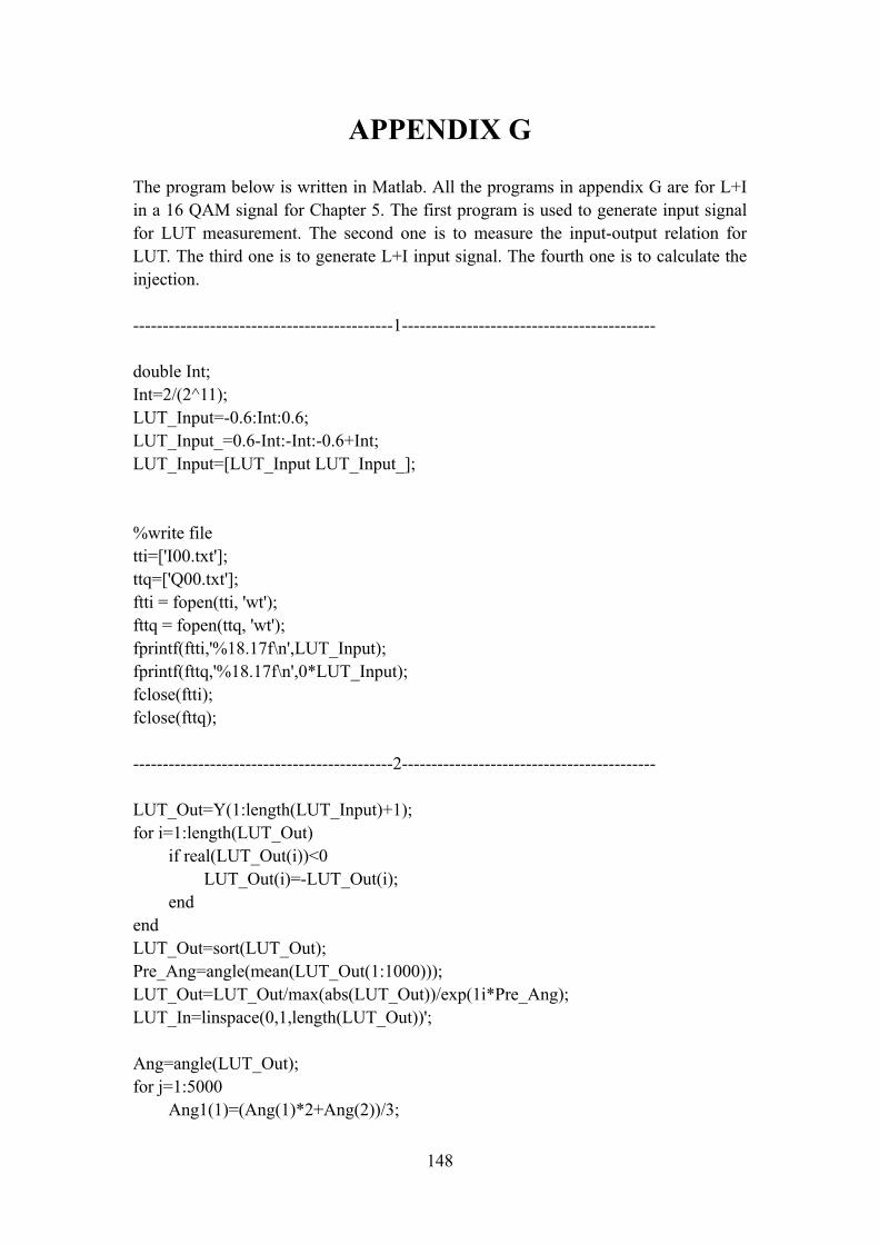
APPENDIX G The program below is written in Matlab. All the programs in appendix G are for L+I in a 16 QAM signal for Chapter 5. The first program is used to generate input signal for LUT measurement. The second one is to measure the input-output relation for LUT. The third one is to generate L+I input signal. The fourth one is to calculate the injection. --------------------------------------------1------------------------------------------- double Int; Int=2/(2^11); LUT_Input=-0.6:Int:0.6; LUT_Input_=0.6-Int:-Int:-0.6+Int; LUT_Input=[LUT_Input LUT_Input_]; %write file tti=['I00.txt']; ttq=['Q00.txt']; ftti = fopen(tti, 'wt'); fttq = fopen(ttq, 'wt'); fprintf(ftti,'%18.17f\n',LUT_Input); fprintf(fttq,'%18.17f\n',0*LUT_Input); fclose(ftti); fclose(fttq); --------------------------------------------2------------------------------------------- LUT_Out=Y(1:length(LUT_Input)+1); for i=1:length(LUT_Out) if real(LUT_Out(i))<0 LUT_Out(i)=-LUT_Out(i); end end LUT_Out=sort(LUT_Out); Pre_Ang=angle(mean(LUT_Out(1:1000))); LUT_Out=LUT_Out/max(abs(LUT_Out))/exp(1i*Pre_Ang); LUT_In=linspace(0,1,length(LUT_Out))'; Ang=angle(LUT_Out); for j=1:5000 Ang1(1)=(Ang(1)*2+Ang(2))/3;
148

if abs(Ang1(1))>abs(Pre_Ang)/100 Ang1(1)=Ang1(1)/100; end for i=2:length(Ang)-1; Ang1(i)=(Ang(i-1)+Ang(i)+Ang(i+1))/3; if i<700&&abs(Ang1(i))>abs(Pre_Ang)/100 Ang1(i)=Ang1(i)/100; end end Ang1(length(Ang))=(Ang(length(Ang))*2+Ang(length(Ang)-1))/3; Ang=Ang1; end Ang=Ang-Ang(1); subplot(1,2,1); plot(abs(LUT_In),abs(LUT_Out)); hold on; plot(abs(LUT_Out),abs(LUT_In),'r'); title('AM/AM') subplot(1,2,2); plot(abs(LUT_In),Ang); hold on; plot(abs(LUT_Out),-Ang,'r'); title('AM/PM') for i=1:length(LUT_Out) LUT_In(i)=LUT_In(i)/(exp(1i*Ang(i))); LUT_Out(i)=abs(LUT_Out(i)); end --------------------------------------------3------------------------------------------- for j=0:9 %Open file tti=['I0' num2str(j) '.txt']; ttq=['Q0' num2str(j) '.txt']; %cubic injection Inject=Input_Mod.*Input_Mod.*conj(Input_Mod); Inject_fft=fft(Inject); for i=1:500 if abs(Inject_fft(i))<0.1 Inject_fft(i)=0.1*Inject_fft(i)/abs(Inject_fft(i)); end end
149

%sideband elimination Inject_fft(91:410)=0; %inband elimination Inject_fft(1:30)=0; Inject_fft(471:500)=0; %brick wall Inject_fft_w=0.15*ones(500,1); %sideband elimination %Inject_fft_w(111:390)=0; Inject_fft_w(191:310)=0; %inband elimination Inject_fft_w(1:30)=0; Inject_fft_w(471:500)=0; Inject_Amp=0; Inject_fft=Inject_fft_w*exp(2i*pi*(j/10))*Inject_Amp+Inject_fft_w.*Filter1.';%+Inject_fft_w.*Filter2.';%+Inject_fft.*Filter.'*0.3; Inject=ifft(Inject_fft); Input_Mod_temp=Input_Mod; Input_Mod=Input_Mod+Inject; for i=1:length(Input_Mod) j=1; while ((LUT_Out(j)<abs(Input_Mod(i)/0.6))&&(j<length(LUT_Out))); j=j+1; end % in the range for LUT if (j<=length(LUT_Out)) Mod=(abs(Input_Mod(i)/0.6)-LUT_Out(j-1))/(LUT_Out(j)-LUT_Out(j-1)); Input_LUT(i,1)=(LUT_In(j-1)+Mod*(LUT_In(j)-LUT_In(j-1)))*0.6*exp(1i*angle(Input_Mod(i))); else % out of range for injection slope=(mean(LUT_In(round(0.9*length(LUT_In)):length(LUT_In)))-LUT_In(length(LUT_In)))/(mean(LUT_Out(round(0.9*length(LUT_Out)):length(LUT_Out)))-1);
150

Input_LUT(i,1)=(abs(Input_Mod(i)/0.6)-1)*slope*0.6+Input_Mod; if Input_LUT(i,1)>1 Input_LUT(i,1)=1; end end end Input_Mod=Input_Mod_temp; ftti = fopen(tti, 'wt'); fttq = fopen(ttq, 'wt'); fprintf(ftti,'%18.17f\n',real(Input_LUT)); fprintf(fttq,'%18.17f\n',imag(Input_LUT)); fclose(ftti); fclose(fttq); end plot(Input_LUT); axis([-1,1,-1,1]); xlabel([dec2hex(Code)';dec2bin(Code,4)']); --------------------------------------------4------------------------------------------- Symbol_length=50; Points_Symbol=10; for File_Index=0:9 load([num2str(File_Index),'.mat']); Covariance=xcov(abs(Input_Mod),abs(Y(1:500))); [M,Time_delay]=max(Covariance); j=File_Index+1; Out(j,:)=Y(Symbol_length*Points_Symbol*2-Time_delay:Symbol_length*Points_Symbol*3-Time_delay-1); In=Input_Mod.'; Length=length(In); In_fft=fft(In)/Length; Out_fft=fft(Out(j,:))/Length; if (File_Index==0) Gain=mean(abs(Out_fft(10:20)./In_fft(10:20))); end %Cubic_ref=(In).*(In).*conj(In); %Cubic_ref_fft=fft(Cubic_ref)/Length; %Cir(j,:)=(Out_fft-Gain*In_fft)./Cubic_ref; Cir(j,:)=fft(Out(j,:)-Gain*In)/Length; end %finding left circle
151

for fre=1:500; Cov(fre)=0; if ((fre>=31&&fre<=190)||(fre>=311&&fre<=470)) Pos=Cir(:,fre); Num_Cir=0; for i=1:8 for j=i+1:9 for k=j+1:10 a=2*(real(Pos(j))-real(Pos(i))); b=2*(imag(Pos(j))-imag(Pos(i))); c=(real(Pos(j)))^2+(imag(Pos(j)))^2-(real(Pos(i)))^2-(imag(Pos(i)))^2; d=2*(real(Pos(k))-real(Pos(j))); e=2*(imag(Pos(k))-imag(Pos(j))); f=(real(Pos(k)))^2+(imag(Pos(k)))^2-(real(Pos(j)))^2-(imag(Pos(j)))^2; Num_Cir=Num_Cir+1; x(Num_Cir)=(b*f-e*c)/(b*d-e*a)+1i*(d*c-a*f)/(b*d-e*a); end end end Center=mean(Pos); Cov(fre)=cov(x)^0.5/mean(abs(Pos(:)-mean(x))); Gain_need=abs(Center)/mean(abs(Pos(:)-Center)); i=1; while (angle((-Center)/(Pos(i)-Center))<0)||(angle((-Center)/(Pos(mod(i,10)+1)-Center))>0) i=i+1; end a=angle((-Center)/(Pos(i)-Center)); b=angle((Pos(mod(i,10)+1)-Center)/(Pos(i)-Center)); Phase_need=(i-1+a/b)/10; if (Gain_need>2) Filter(fre)=Gain_need*exp(2i*pi*Phase_need); else Filter(fre)=Gain_need*exp(2i*pi*Phase_need); end %if (Cov(fre)>4) % Filter(fre)=Filter(fre)/Cov(fre); %end else Filter(fre)=0; end end
152

Publish Papers
M. Xiao and P. Gardner, "Digital Baseband Injection Techniques to Reduce Spectral Regrowth in Power Amplifier," IEEE MTT-S Int. Microwave Symp. Dig., Atlanta, Georgia, June 2008
M. Xiao and P. Gardner, "Characterisation, analysis and injection of two-tone
third-order intermodulation products in an amplifier," IET Microwaves, Antennas & Propagation, vol. 3, issue 3, pp. 443-455, 2009.
M. Thian, M. Xiao, and P. Gardner, "Digital Baseband Predistortion Based
Linearized Broadband Inverse Class-E Power Amplifier," IEEE Transactions on Microwave Theory and Techniques, vol. 57, issue 2, pp. 323 - 328, Feb, 2009.
153