NOVEL ECONOMICAL EMISSION MONITORING · PDF fileYour file Votre reference ISBN: 978-0-494-93511-8 ... 4.2.1 Lasing Assembly ... 4.2.2 Test GasDelivery System

NOVEL ECONOMICAL EMISSION MONITORING TECHNOLOGY FOR

LIQUID STORAGE TANKS (LST)

by

Clifton Pereira

A thesis submitted to The Faculty o f Graduate Studies and Research

in partial fulfilment of the degree requirements of

Master of Applied Science in Mechanical Engineering

Ottawa-Carleton Institute for

Mechanical and Aerospace Engineering

Department of Mechanical and Aerospace Engineering

Carleton University

Ottawa, Ontario, Canada

July 2012

Copyright ©2012 - Clifton Pereira

1+1Library and Archives Canada

Published Heritage Branch

Bibliotheque et Archives Canada

Direction du Patrimoine de I'edition

395 Wellington Street Ottawa ON K1A0N4 Canada

395, rue Wellington Ottawa ON K1A 0N4 Canada

Your file Votre reference

ISBN: 978-0-494-93511-8

Our file Notre reference ISBN: 978-0-494-93511-8

NOTICE:

The author has granted a nonexclusive license allowing Library and Archives Canada to reproduce, publish, archive, preserve, conserve, communicate to the public by telecommunication or on the Internet, loan, distrbute and sell theses worldwide, for commercial or noncommercial purposes, in microform, paper, electronic and/or any other formats.

AVIS:

L'auteur a accorde une licence non exclusive permettant a la Bibliotheque et Archives Canada de reproduire, publier, archiver, sauvegarder, conserver, transmettre au public par telecommunication ou par I'lnternet, preter, distribuer et vendre des theses partout dans le monde, a des fins commerciales ou autres, sur support microforme, papier, electronique et/ou autres formats.

The author retains copyright ownership and moral rights in this thesis. Neither the thesis nor substantial extracts from it may be printed or otherwise reproduced without the author's permission.

L'auteur conserve la propriete du droit d'auteur et des droits moraux qui protege cette these. Ni la these ni des extraits substantiels de celle-ci ne doivent etre imprimes ou autrement reproduits sans son autorisation.

In compliance with the Canadian Privacy Act some supporting forms may have been removed from this thesis.

While these forms may be included in the document page count, their removal does not represent any loss of content from the thesis.

Conformement a la loi canadienne sur la protection de la vie privee, quelques formulaires secondaires ont ete enleves de cette these.

Bien que ces formulaires aient inclus dans la pagination, il n'y aura aucun contenu manquant.

Canada

The undersigned recommend to

the Faculty of Graduate Studies and Research

acceptance o f the thesis

NOVEL ECONOM ICAL EM ISSION M ONITORING TECHNOLOGY FOR

LIQUID STORAGE TANKS (LST)

Submitted by Clifton Pereira

in partial fulfilment of the requirements for the degree of

M aster of Applied Science in M echanical Engineering

Dr. Matthew Johnson, Thesis Supervisor

Dr. Metin Yaras, Chair, Department o f Mechanical and Aerospace Engineering

Carleton University

2012

ii

Abstract

A low-cost Mid Infrared (IR) direct absorption spectroscopic cross correlation

velocimetry (DAS-CCV) technique for hydrocarbon line flux measurements has been

developed and tested experimentally. This research was conducted as the proof-of-

concept stage in the development of an economical sensor system to quantify volatile

organic compound (VOC) emissions from liquid storage tanks (LST). A Mid-IR

(3.392 pm) Helium Neon laser was used to create two vertically displaced laser lines that

were used to measure instantaneous, path integrated concentrations through a buoyant

hydrocarbon (methane) plume. From these measurements, the fluctuating component of

the concentration signals, corresponding to the eddy flow within the plume, were

compared using a statistical technique known as CCV to estimate the velocity o f the

hydrocarbon plume. From experiments using a flow-through spectroscopic cell (with a

controlled path length) filled with methane diluted in air, the sensor was able to achieve

accurate measurements of 300 - 900 ppm m at a maximum uncertainty o f 1.35%. The

analysis of the noise performance of the in-lab experimental apparatus demonstrated a

theoretical sensor detectivity limit o f 2.22 parts per million-meter (ppm m). DAS-CCV

experiments were conducted using both air-methane and helium-methane mixtures.

Results showed that line flux measurements were achieved with uncertainties of 2-7.5%

(air-CH4 ) and 5-19% (helium-CH4). From Schlieren imaging, it was determined that the

higher uncertainties were attributable to the 39.1 mm beam spacing which allowed for

noticeable diffusion of the eddies (particularly for the helium mixtures) as they traversed

the two beams. Overall, the proof-of-concept system demonstrated that the DAS-CCV

technique is a viable approach and the traverse tests demonstrated the potential o f a full

scale multiline, gridded sensor to measure the emissions released by LSTs with good

accuracy and for a relatively low monetary investment.

Acknowledgements

This thesis would not have been possible without the support o f my supervisor, Dr.

Matthew Johnson from Carleton University. His encouragement and patience has kept

me going throughout this journey and I would like to formally thank him for this research

opportunity, where I gained skills and experience that will be invaluable throughout my

career.

I would like to thank my fellow co-workers of Dr. Johnson’s research group that

have helped me with my research and made the lab environment bearable. I would like

to specifically thank, in no particular order, Graham Ballachey, Stephen Schoonbaert,

Brian Crosland, David Tyner, Jan Gorski, Ian Joynes, Carol Bereton, and Darcy Corbin.

I would also like to thank the members o f the ABL lab, for being my second home away

home, for cheering me up during the darker days, lending me an idea or two when I had

hit a wall and celebrating with me during the lighter days. I would specifically like to

thank, in no particular order, Kyle Klumper, Kyle Chisholm, Aliasgar Morbi, Ahmed

Sabry, Richard Berenek, Angela Schuegraf, Jennifer Baba and Dr. Ahmadi.

I would like to thank the staff of the department o f mechanical and aerospace

engineering, specifically, Marlene Groves, Christie Egbert, Nancy Powell, Neil

McFadyen, Bruce Johnston, Alex Proctor and Kevin Sangster for all their help and their

boundless patience during my graduate career.

I would also like to thank my friends in Ottawa and Toronto, who kept me sane

throughout my graduate studies and reminded me there was a life outside o f the lab. I

would like to specifically thank, Omer Lari, Xiong Mai, Natsuki Okabe, Kanako Oshima,

John Dahms, Peter Berg, Tina Su, Becky Yuen and Michael Troung. Finally, I would

like to thank my parents and my sisters, for their understanding and support throughout

my graduate studies.

Table of ContentsAbstract......................................................................................................................................... iii

Acknowledgements...................................................................................................................... iv

List of Tables................................................................................................................................ ix

List of Figures...............................................................................................................................xi

Nomenclature............................................................................................................................ xvii

Chapter 1 Introduction.......................................................................................................... 22

1.1 M otivation.....................................................................................................................22

1.2 Designs o f Liquid Storage Tanks (LSTs)................................................................. 23

1.2.1 Fixed Roof Tank................................................................................................. 23

1.2.2 Floating Roof T anks............................................................................................ 24

1.2.3 Horizontal Storage Tanks....................................................................................29

1.3 Previous Comparisons o f Estimated Emissions from Liquid Storage Tanks with

Field Measurements using Differential Absorption LIDAR (D IA L).................................. 30

1.4 Experimental Obj ecti ve...............................................................................................33

1.5 Organization o f Thesis................................................................................................33

Chapter 2 Remote Sensing of Evaporative Losses from Liquid Storage T anks 35

2.1 Absorption Spectroscopy...........................................................................................35

2.1.1 Direct Absorption Spectroscopy (D A S).......................................................... 36

2.1.2 Wavelength-Modulation Spectroscopy (W M S)...............................................36

2.1.3 Differential Absorption Light Detection and Ranging (DIAL)......................37

2.1.4 Solar Occultation Flux (SOF) Method............................................................... 38

2.2 Velocity Measurement Techniques using Absorption Spectroscopy.....................39

2.2.1 Doppler Shift Velocity Measurement................................................................ 39

2.2.2 Cross Correlation Velocity Measurement.........................................................40

2.3 Selection o f Absorption Spectroscopic and Velocity Techniques........................ 41

2.3.1 Selection o f Absorption Spectroscopy W avelength....................................... 42

Chapter 3 Background on MID-IR Absorption Spectroscopy and Technology........... 47

3.1 Mid-IR Absorption Spectroscopy..............................................................................47

3.1.1 Measurement of Volume Fraction using DAS................................................. 49

3.1.2 Measurement o f a Plume’s Velocity through CCV with Mid-IR DAS 51

3.1.3 Mid-IR Laser Source Survey..............................................................................53

3.1.4 Helium Neon Lasers............................................................................................ 54

3.1.5 Lead Salt Diode Lasers....................................................................................... 55

3.1.6 Quantum Cascade Lasers.................................................................................... 56

3.1.7 Difference Frequency Generation (DFG) L aser.............................................. 57

3.1.8 Optical Parametric Oscillators (O PO )...............................................................58

3.1.9 Motivation and Selection o f the Mid IR Lasing Source................................. 59

3.2 Mid-IR Detectors.......................................................................................................... 60

3.2.1 Motivation and Selection of the Mid IR detector............................................ 63

Chapter 4 Experimental Setup.............................................................................................. 65

4.1 General Approach........................................................................................................ 65

4.2 VOC Measurement System.........................................................................................6 6

4.2.1 Lasing Assembly...................................................................................................67

4.2.2 Test GasDelivery System.................................................................................... 72

4.2.3 Detector Assembly............................................................................................... 75

4.3 Optical Power Conversion Electronics..................................................................... 76

4.4 Flow Visualization Apparatus.....................................................................................78

4.5 Experimental Methodology........................................................................................82

4.5.1 Line-Averaged Concentration M easurements................................................. 82

4.5.2 CCV methodology............................................................................................... 87

4.5.3 Mass Flow Transverse test..................................................................................91

4.5.4 Schlieren Imaging Methodology........................................................................ 91

Chapter 5 Results....................................................................................................................94

5.1 VOC Sensor Response................................................................................................ 94

5.1.1 T ransient Response.............................................................................................. 94

5.1.2 Random Noise Distribution...............................................................................95

5.2 Concentration Measurement Sensitivity................................................................... 98

5.3 CCV and Methane Flux Measurements.................................................................. 102

5.3.1 Path integrated concentration measurements.................................................103

5.3.2 C C V ......................................................................................................................105

5.3.3 Line Flux Measurements....................................................................................112

5.3.4 Mass flow measurements from traverse te sts .................................................114

5.4 Schlieren Im aging..................................................................................................... 116

5.4.1 Buoyant eddy behaviour...................................................................................116

5.4.2 Plume path length...............................................................................................119

5.5 Cost-effective critique................................................................................................121

Chapter 6 Conclusions and Future W ork..........................................................................123

6.1 Conclusions................................................................................................................. 123

6.2 Future W ork................................................................................................................ 125

6.2.1 Detector-Amplifier Noise Performance...........................................................125

6.2.2 CCV Optimal Beam spacing............................................................................. 125

6.2.3 Hydrocarbon speciation...................................................................................126

6.2.4 Multi-line CCV ....................................................................................................127

References.................................................................................................................................. 128

Appendix A Mechanisms o f Evaporative Losses from Liquid Storage T ank................. 133

A. 1 Working Losses of Liquid Storage Tanks............................................................. 133

A.2 Standing Losses o f Liquid Storage Tanks............................................................. 133

A.2.1 Standing Losses of Floating Roof Storage T anks.........................................134

A.2.2 Standing Losses of Fixed Roof and Horizontal T a n k s ..................................145

Appendix B Current Models for Estimating Emissions from Liquid Storage Tank.... 144

B.l Emission Factors of Floating Roof Tanks...............................................................144

B. 1.1 Standing loses of Floating Roof T anks.........................................................145

B .l.2 Working loses of Floating Roof T anks.........................................................151

B. 1.3 Fugitive Emission Factors of “Landed” Floating Roof Tanks...................152

B.2 Emission Factors of Fixed Roof Tanks and Horizontal T anks............................. 157

B.2.1 Standing losses of Fixed Roof and Horizontal T anks................................ 157

B.2.2 Working losses o f Fixed Roof and Horizontal Tanks................................159

Appendix C Amplifier PCB D esign...................................................................................161

Appendix D Beam Steering Tests....................................................................................... 163

List of Tables

Table 1.1: Summary of Fugitive Emissions at Alberta Gas Plants as Measured with DIAL

(Chambers, 2004)........................................................................................................................ 31

Table 1.2: Measured vs. Estimated VOC Emissions a sweet gas plant (Chambers, 2004)

........................................................................................................................................................ 31

Table 1.3: Measured vs. Estimated VOC Emissions a sour gas plant (Chambers, 2004) 31

Table 2.1: Canister Sample from Condensate Tank Area at the Sour Gas Plant

(Chambers, 2004)........................................................................................................................ 43

Table 2.2: The Optimal Spectral Regions (OSR) for the VOC emissions from an EFRT

(AIST, 2010; Pouchert, 1981)....................................................................................................45

Table 3.1: Summary of Commercially Available Mid-IR Laser Source Survey (Pashotta,

2008; Tittel, Richter, & Fried, 2003; Klingbeil, 2007; Cockbum, 2006; Kosterev, et al.,

2008; Springholz, Schwarzl, & Heiss, 2006; Weber, 1999)..................................................60

Table 3.2: Theoretical SNR’s for PV HgCgTe....................................................................... 64

Table 4.1: Relative uncertainties o f the measured/calculated parameters...........................87

Table 5.1: Detector Assemblies transient response characteristics..................................... 94

Table 5.2: Time averaged concentration sensitivity...............................................................98

Table 5.3: Relative uncertainties of the measured/calculated parameters.........................101

Table 5.4: CCV Experimental Study Breakdown................................................................. 102

Table 5.5: The relative uncertainties of the mean path integrated concentration of

methane.......................................................................................................................................104

Table 5.6: The relative uncertainties of the measured line flux of CH4 .......................... 114

Table 5.7: Methane mass flow measurements using a traverse.........................................116

Table 5.8: The average plume path length measured from the post-processed Schlieren

images (Units are in m etres).................................................................................................... 120

Table 5.9: Detailed Cost Breakdown of the Developed Sensor System............................ 122

Table B .l: Rim seal loss factors (EPA, 1995)..................................................................... 147

Table B.2: Clingage factors (EPA, 1995)............................................................................. 152

x

List of Figures

Figure 1.1: Typical Fixed Roof Tank (EPA, 1995)................................................................24

Figure 1.2: External Floating Roof (EFRT) - Double-deck Type (Pasley& Clark, 2000)26

Figure 1.3: External Floating Roof Tank (EFRT) - Pontoon Type Roof (EPA, 1995).... 27

Figure 1.4: Internal Floating Roof Tank (IFRT) (Land and Marine Project Engineering

Ltd., 2011).................................................................................................................................... 28

Figure 1.5: The honeycomb type roof construction (Long & Gamer, 2004)..................... 28

Figure 1.6: Typical underground horizontal storage tank (EPA, 1995)..............................29

Figure 1.7: Typical aboveground horizontal storage tank (EPA, 1995)..............................30

Figure 2.1: (left) FFT o f the detector’s signal with the 2f bandpass filter window; (right)

the 2 f component of the detectors signal that is proportional to target gas’s concentration

(Svensson et al., 2008)................................................................................................................ 37

Figure 2.2: DIAL Operational Methodology (Spectrasyne Ltd., 2010)..............................38

Figure 2.3: Illustration of the SOF method (Mellqvist et al., 2006).................................... 39

Figure 2.4: General methodology of Velocity and Density measuring techniques

(Mohamed & Lefebvre, 2009).................................................................................................. 40

Figure 2.5: Example of measuring the velocity of a turbulent je t with a CCV Probe. Two

thermocouples placed d (cm) apart (Rockwell, Rangwala, & Klein, 2009)........................ 41

Figure 2.6: EFRT Headspace vapour composition and concentrations (Picard, 2009).... 44

Figure 2.7: Transmission spectrum of Pentane (AIST, 2010).............................................. 45

Figure 2.8: Transmission spectrum of Hexane (AIST, 2010)............................................... 46

Figure 3.1: Variation of transmittance o f 0.2% methane in air for different pressures at a

fixed temperature o f 300 K (Adapted from HITRAN 2008)................................................49

XI

Figure 3.2: Variation of transmittance of 0.2% methane in air for different temperatures

at a fixed pressure o f 101.3 kPa (Adapted from HITRAN 2008).........................................49

Figure 3.3: A breakdown of individual maximum atmospheric absorption across the OSR

for an 80cm path length at STP..................................................................................................51

Figure 3.4: Example of CCV on plume fluctuation; (a) Example of two transient signals;

(b) The Cross correlation parameter as a function o f time delays, seen maximized at 2

seconds.......................................................................................................................................... 52

Figure 3.5: Mid-IR Spectroscopic Sources and their operating ranges (Tittel et al., 2003)

........................................................................................................................................................ 54

Figure 3.6: Schematic o f HeNe laser (Thorlabs, 2011)......................................................... 55

Figure 3.7: Schematic o f DFG laser source (Tittel, Richter, & Fried, 2003)..................... 57

Figure 3.8: Optical Parametric Oscillation Lasing Methodology (Tittle et al., 2003).......59

Figure 3.9: The Operation Wavelength (A) and the Frequency Bandwidth (B) of

commercially available Mid-IR detectors; the Blue region indicates (see A) the

operational wavelength o f interest for VOCs(Klingbeil, 2007)............................................ 61

Figure 3.10: Comparison of the D* of various commercially available IR detectors

(Piotrowski & Rogalsk, 2007)...................................................................................................63

Figure 3.11: Schematic of simplified plume............................................................................64

Figure 4.1: Schematic o f Proposed Experimental Apparatus to Measure a Line Flux

through cross-correlation techniques; BS - Beam splitter, M - Turning mirror, CL -

Collimating lens...........................................................................................................................65

Figure 4.2: Schematic o f proposed experimental apparatus to determine concentration

sensitivity; BS - Beam splitter, M - Turning mirror, CS - Collimating len s ...................... 6 6

Figure 4.3: Experimental apparatus (with plume generator)................................................ 6 6

Figure 4.4: Lasing assembly o f the VOC measurement sensor............................................ 6 8

Figure 4.5: HeNe Laser - 30 mm cage alignment adapter....................................................6 8

xii

Figure 4.6: Spectral transmission curve of (Left) IR Neutral Density Filter (OD=0.3);

(Right) Specialized pellicle beam splitter................................................................................ 70

Figure 4.7: (Left) Spectral transmission of f=40mm CaFb Plano-convex lens; (Right)

Spectral responsivity of the PVI-3.4 detector..........................................................................70

Figure 4.8: Spectral Reflectance curve for the gold plated mirror (Thorlabs Ltd., 2011) 71

Figure 4.9: (Left) Thermistor’s electrical circuit; (Right) Calibrated temperature response

curve of the Omega therm istor................................................................................................. 72

Figure 4.10: Schematic test gas delivery system and its components................................. 72

Figure 4.11: Example of a calibration curve for Brooks M FC............................................. 73

Figure 4.12: Plume generator for CCV spectroscopic study................................................. 74

Figure 4.13: Spectroscopic flow-through cell......................................................................... 74

Figure 4.14: Detector Assembly of the VOC measurement Sensor.................................... 75

Figure 4.15: Stage 1- Transimpedance amplifier with variable gain................................... 76

Figure 4.16: Stage 2 -ACextraction circuit with fixed (X2) gain.........................................77

Figure 4.17: Stage 3 - AC amplification with variable gain..................................................78

Figure 4.18: Custom “in-house built” detector amplifier......................................................78

Figure 4.19: A simple lens-based Schlieren setup (Atcheson, 2007).................................. 79

Figure 4.20: Z-type Schlieren imaging system (Top-view)...................................................80

Figure 4.21: Parabolic mirrors used for Schlieren imaging system......................................81

Figure 4.22: (Left) Knife-edge assembly; (Right) Schlieren Image and acquisition camera

82

Figure 4.23: Mid-IR DAS methodology.................................................................................. 82

Figure 4.24: Molar Absorption coefficient of CH4 distribution across the mid-IR OSR;

the approximate location of the HeNe laser beams FWHM is highlighted in dashed red

lines (HITRAN, 2008)................................................................................................................8 6

xiii

Figure 4.25: The methodology of the experimental validation of CCV via direct

absorption spectroscopy............................................................................................................. 8 8

Figure 4.26: Example of t for Air -M ethane Test.................................................................. 89

Figure 4.27: Example of calculated CL for both laser/detector lines (Left) and the Rxy

coefficient(Right)........................................................................................................................ 90

Figure 4.28: Schematic of the traverse test to measure the total mass flow of the plume 91

Figure 4.29: Example of the image processing used to gather spatial information of the

plume............................................................................................................................................. 92

Figure 4.30: Example of the combined binary image used to estimate length scales in the

plume............................................................................................................................................. 93

Figure 5.1: Detector response to a step change in incident laser radiation from 0 to 100%

of the laser power........................................................................................................................ 95

Figure 5.2: Power spectrum distribution o f the raw signals of(a) top detector and (b)

bottom detector; The AC (60 Hz) noise and its n order harmonics are highlighted in

dashed red boxes......................................................................................................................... 96

Figure 5.3: (a) Power spectrum of the detector signal; (b) Power spectrum of the

normalized detector signal. The AC (60 Hz) noise and its n order harmonics are

highlighted in dashed red boxes................................................................................................ 97

Figure 5.4: Measurements of the x C/74 for step inputs of 0 to (a) 0.05 and (b) 0.1........99

Figure 5.5: Measurements o f the x C774 of a Multi-Step concentration tests from 0.05 -

0.95...............................................................................................................................................100

Figure 5.6: Measured vs. Set x C/74 along with the associated measurement uncertainty

101

Figure 5.7: Relative measured uncertainty as a function of set x C /74............................102

Figure 5.8: Measured path integrated concentration of methane for Air-CH4 case study

...................................................................................................................................................... 104

xiv

Figure 5.9: Measured path integrated concentration of methane for the Helium-CH^ase

study............................................................................................................................................ 105

Figure 5.10: Standard deviation of the measured velocity vs. the CCV sample period for

Air-CH4 mixtures at the (a) minimum and (b) maximum of experimental air flow range

...................................................................................................................................................... 107

Figure 5.11: Standard deviation o f the measured velocity vs. the CCV sample period for

Helium-CFU flows at the (a) minimum and (b) maximum of experimental helium flow

range............................................................................................................................................ 108

Figure 5.12: Example of a histogram of CCV extracted time delay for a test point 109

Figure 5.13: (Left) the path integrated concentration of the (red) lower and (blue) upper

detectors and the (Right) Rxy time lag distribution for the corresponding 4000 samples for

a Helium-Methane (1.5/0.1 SLPM) test ru n ..........................................................................109

Figure 5.14: Measured eddy velocities of the Air-CfL plume as a function o f methane

mass flux.....................................................................................................................................I l l

Figure 5.15: Measured eddy velocities for the Helium-CFLcase study as a function of the

methane mass flux......................................................................................................................1 1 1

Figure 5.16: Measured eddy velocities of the Helium-CFL case study as a function of the

total mass flux............................................................................................................................ 1 1 2

Figure 5.17: Measured Line Flux o f Methane for the Air-CH4 mixtures......................... 113

Figure 5.18: Measured Line Flux o f Methane for the Flelium-CFL} mixtures..................113

Figure 5.19: Path integrated concentration measurements across the traverse path length

...................................................................................................................................................... 115

Figure 5.20: Plume eddy velocity measurements across the traverse path length............116

Figure 5.21: Time lapsed images (At=0.1s) of air (at 0.5 SLPM) and CFL(at 0.5SLPM)

118

xv

Figure 5.22: Time lapsed images (At=0.1s) o f air (at 1.5 SLPM) and CH4 (at 0.5 SLPM)

118

Figure 5.23: Time lapsed images (At=0.1s) o f helium (at 1.5 SLPM) and CH4 (at 0.5

SLPM)......................................................................................................................................... 119

Figure 5.24 : Time lapsed images (At=0.1s) of helium (at 4.5 SLPM) and CH4 (at 0.5

SLPM)......................................................................................................................................... 119

Figure 5.25: Plume-Laser path length measurement of helium (at 4.5 SLPM) and CH4 (at

0.5 SLPM); (left) the intensity distribution across the laser beam spacing mid-point

(y=l 55, x=0 - 424); (right) Average of a 100 post-processed Schlieren images 120

Figure A .l: Deck rim seals (EPA, 1995).............................................................................. 135

Figure A.2: Typical Floating Roof Deck Fittings(EPA, 1995).......................................... 138

Figure A.3: Typical Floating Roof Deck Fittings (EPA, 1995)......................................... 140

Figure A.4: Slotted guide pole deck fitting (EPA, 1995)................................................... 141

Figure A.5: Different configurations of a “landed” internal roof (EPA, 1995).............. 142

Figure A.6 : Section view of a typical underground horizontal storage tank (EPA, 1995)

...................................................................................................................................................... 143

Figure C .l: PCB Schematic..................................................................................................... 161

Figure C.2: PCB Layout...........................................................................................................162

xvi

Nomenclature

Symbol Description First usage

Ad Active detector area [cm2] Equation (3.6)

Bi Systematic uncertainty o f variable Equation (4.4)

C Concentration [mol/m3] Equation (3.1)

Path integrated concentration for the n detector CLn(t) Equation (3.4)

[mol/m2]

Ct Concentration o f the o f the ith gas [mol/ m3] Equation (3.2)

D Detectivity [cm-Hz1/2 -VT1] Equation (3.6)

Abeam Laser Beam separation [m] Equation (4.19)

I Power of the transmitted radiation [W] Equation (3.1)

I0 Power o f the incident radiation [W] Equation (3.1)

Detector signal that has normalized using the reference h l h e f Equation (4.1)

detector [-]

The base detector signal that has normalized using the V W | 0 Equation (4.1)

reference detector with no absorption [-]

L Path length through the target gas [m] Equation (3.1)

m CHJ Line flux o f methane [g/s-m] Equation (4.21)

MWCh4 Molecular weight of methane [g/mol] Equation (4.21)

N The total number of discrete samples i.e. the sample Equation (3.5)

period [-]

PA Barometric pressure [Pa] Equation (3.1)

P, Power of the incident radiation [W] Equation (3.8)

Pt Precision uncertainty of variable Xt Equation (4.4)

Q l p m Volumetric flow rate [LPM] Equation (4.12)

Q s l p m Volumetric flow rate in STP conditions [SLPM] Equation (4.12)

Rxy Cross correlation parameter [-] Equation (3.5)

R Universal gas constant [J/K-mol] Equation (3.3)

R Result Equation (4.3)

T Temperature [K] Equation (3.1)

^ , 9 5 % 95 % confidence t- value from the student’s distribution Equation (4.5)

UXi Uncertainty associated with variable X, Equation (4.3)

Vccv Velocity from the CCV algorithm [m/s] Equation (4.19)

Defined as orthogonal to the laser light axis and thex-axis

plume flow direction

Defined as parallel to the laser light axis and orthogonaly-axis

to the plume flow direction

Defined as orthogonal to the laser light axis and parallelz-axis

to the plume flow direction

A / Frequency bandwidth of the detector [Hz] Equation (3.6)

AtCcv Time delay from CCV algorithm [s] Equation (4.19)

xviii

GreekSymbols

a Absorbance measured of the target gas [-] Equation (3.1)

a mixAbsorbance measured of the multi-component gas

mixture [-]Equation (3.2)

a (T ,P ,v )Molar absorption coefficient as a function temperature,

pressure and wavelength [m2 /mol]Equation (3.1)

f f i C r P v )

Molar absorption coefficient of the ith gas as a function

temperature, pressure and wavelength [m2/mol]Equation (3.2)

°CH4Molar absorption coefficient of the methane [m2 /mol] Equation (4.2)

T Response time of the detector [s] Equation (3.7)

TrTransmittance of the target gas [-] Equation (3.1)

TRmlx

V

Transmittance of the multi-component gas mixture [-]

Wavelength [pm]

Equation (3.2)

Equation (3.1)

XCH4Measured volume fraction of methane [-] Equation (3.3)

Acronyms

A/D Analog to digital Section (5.4.1)

AC Alternating Current Section (3.3.1)

AIST Advanced Industrial Science and Technology Section (2.3.1)

API American Petroleum Institute Section (1.1)

AR Anti-reflective Section (4.2.1)

BS Beam splitter Section (4.1)

CCV Cross correlation velocimetry Section (2.2.2)

CL Collimating lens Section (4.1)

CNC Computer numerical control Section (4.2.1)

DAS Direct Absorption Spectroscopy Section (2.1.1)

DAQ Data acquisition Section (4.3)

DC Direct Current Section (3.2.1)

DFG Difference Frequency Generation Section (3.2.4)

DIAL Differential Absorption Lidar Section (1.1)

EFRT External Floating Roof Tanks Section (1.2)

EPA Environmental Protection Agency Section (1.1)

ET etalon Section (3.2.5)

FTIR Fourier Transform InfraRed (spectroscopy) Section (2.3.1)

GHG Greenhouse Gas Section (1.1)

HeNe Helium Neon Section (3.2.1)

HIPPO HIAPER Pole-to-Pole Observations Section (3.2.3)

HITRANHigh- resolution TRANsmission molecular absorption

databaseSection (2.1)

ID Inner diameter Section (4.1)

IFRT Internal Floating Roof Tank Section (1.2)

IR Infrared Section (2.0)

LST Liquid Storage Tank

XX

Section (1.1)

NEP Noise Equivalent Power Section (3.3)

NI National Instruments Section (4.3)

NPT National Physical Laboratory Section (1.4)

OD Optical density Section (4.2.1)

OPO Optical Parametric Oscillators Section (3.2.5)

OPAMPS Operational amplifiers Section (4.3)

OSR Optimal Spectral Region Section (2.1)

PC Photoconductive Section (3.3)

PPLN Periodically Poled Lithium Niobate Section (3.2.4)

PV Photovoltaic Section (3.3)

QCL Quantum Cascade Laser Section (3.2.3)

SLPM Standard litres per minute Section (4.2.2)

SM Semitransparent mirrors Section (3.2.5)

SNR Signal to Noise Ratio Section (2.1.2)

TCEQ Texas Commission on Environmental Quality Section (1.4)

TDL Tunable Diode Laser Section (2.1.1)

TSM Taylor series method Section (4.5.1.1)

UNC Unified coarse Section (4.2.1)

VOC Volatile Organic Carbon Section (1.1)

WMS Wavelength Modulation Spectroscopy Section (2.1.2)

Chapter 1

Introduction

1.1 Motivation

Liquid storage tanks (LST) are cylindrical metallic containers that operate at or very near

atmospheric pressure (typical pressure difference o f no more than a few inches of water).

They are ubiquitous in the petrochemical industry where they are used to store a variety

of organic products (hydrocarbon-based) throughout the production, refining, and

distribution process. The American Petroleum Institute (API) and the United States

Environmental Protection Agency (EPA) estimate that there are on the order o f 700,000

petroleum storage tanks and about 1.3 million underground storage tanks in use in the

United States alone (Myers, 1997).

Liquid storage tanks come in various designs and sizes, but are distinguished

apart from other storage devices (such as pressure vessels) due to their interaction with

the environment through operational fittings (e.g. open vents or pressure relief vents) and

moveable seals. Environment Canada estimates that the emissions generated by liquid oil

storage tanks contribute 2.2 percent o f Greenhouse Gas (GHG) emissions and 31.5

percent of the Volatile Organic Carbon (VOC) emissions generated by the Canadian

upstream oil and gas industry (Picard, 2009); amounting to 0.4% o f national GHG

emissions (Env. Can., 2008) and 9.97% of national VOC emissions (Env. Can. 2010).

As detailed in Appendix A, the emissions from liquid storage tanks generally

occur via three main mechanisms: working losses, standing losses and flashing losses.

Working losses are the emissions that are generated by changes in the liquid level o f the

tank during the filling and emptying process, which push out or draw in gases. Standing

losses (also known as breathing losses) are the emissions that are continually generated

by varying ambient atmospheric conditions (i.e. fluctuations in ambient temperature,22

pressure, and insolent solar radiation causing expansion and contraction o f the vapours

within the tank, or changes in crosswind flow). These are further amplified through

fitting leaks caused by operational wear. Flashing losses occur when organic liquid

experiences a pressure drop causing previously dissolved gasses to be released, as most

commonly occurs when pressurized transmission lines direct multi-component liquids

into an atmospheric pressure storage tank.

Most current methods o f estimating liquid storage tank emissions are based on a

series of semi-empirical algorithms developed by the API and published by the EPA

(1995). These models are widely used due to the lack o f alternative models and the

absence of economical sensor technology for measurement or monitoring. However,

from a brief study conducted by Chambers et al. (2006) on five gas plants in Alberta

using a Differential Absorption Lidar (DIAL), a laser-based optical method that can

remotely measure the concentration o f gases in the atmosphere, it was found that the

measured daily emissions of methane and VOC’s were four to eight times higher than the

emission factor estimates. Unfortunately the DIAL technique is not an ecomically viable

technology and cannot be utilized to measure emissions over longer time-scales (more

than a day) without significant financial investment. Given the significance of VOC and

GHG emissions from liquid storage tanks, there is an obvious need for quantitative

models and measurement techniques that could be employed in reducing these important

sources of fugitive emissions.

1.2 Designs of Liquid Storage Tanks (LSTs)

Liquid storage tank (LST) designs are generally classified based on their roof type and

orientation. There are four main types of storage tanks used in the petrochemical

industry. These are: fixed-roof tanks, Internal Floating Roof Tanks (IFRT), External

Floating Roof Tanks (EFRT), and horizontal tanks.

1.2.1 Fixed Roof Tank

According to the EPA (1995), the most commonly used above ground LST is the fixed

roof tank, which are the least expensive and the minimum acceptable device for the

storage of hydrocarbon-based organic liquids. Figure 1.1 shows a typical fixed-roof tank23

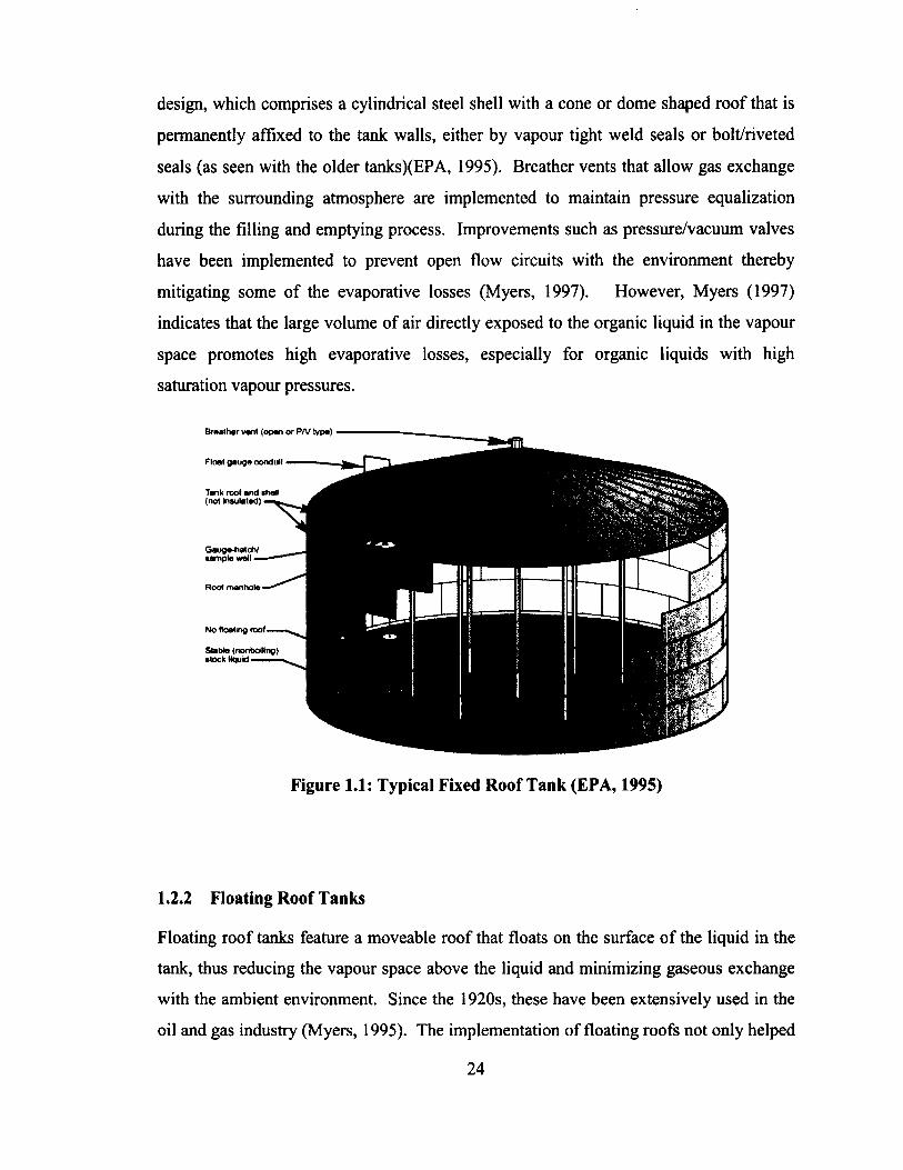
design, which comprises a cylindrical steel shell with a cone or dome shaped roof that is

permanently affixed to the tank walls, either by vapour tight weld seals or bolt/riveted

seals (as seen with the older tanks)(EPA, 1995). Breather vents that allow gas exchange

with the surrounding atmosphere are implemented to maintain pressure equalization

during the filling and emptying process. Improvements such as pressure/vacuum valves

have been implemented to prevent open flow circuits with the environment thereby

mitigating some of the evaporative losses (Myers, 1997). However, Myers (1997)

indicates that the large volume of air directly exposed to the organic liquid in the vapour

space promotes high evaporative losses, especially for organic liquids with high

saturation vapour pressures.

Breather vent (open or P/V type)

Float gauge conduit

Tank roof and shell (not insulated)

Gauge-hatch/ sample well —

Roof manhole -

No floating roof—

Stable (nonbolBng) stock liquid-

•w v - r ' '1

- • ^ 4

Figure 1.1: Typical Fixed Roof Tank (EPA, 1995)

1.2.2 Floating Roof Tanks

Floating roof tanks feature a moveable roof that floats on the surface o f the liquid in the

tank, thus reducing the vapour space above the liquid and minimizing gaseous exchange

with the ambient environment. Since the 1920s, these have been extensively used in the

oil and gas industry (Myers, 1995). The implementation of floating roofs not only helped

24

to reduce the fugitive emissions generated by storage tanks, but also helped to prevent

vapour head space explosions that were quite common for fixed roof storage tanks

(Myers, 1997).

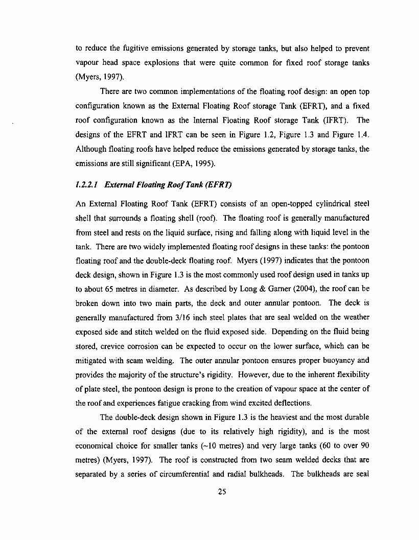
There are two common implementations of the floating roof design: an open top

configuration known as the External Floating Roof storage Tank (EFRT), and a fixed

roof configuration known as the Internal Floating Roof storage Tank (IFRT). The

designs of the EFRT and IFRT can be seen in Figure 1.2, Figure 1.3 and Figure 1.4.

Although floating roofs have helped reduce the emissions generated by storage tanks, the

emissions are still significant (EPA, 1995).

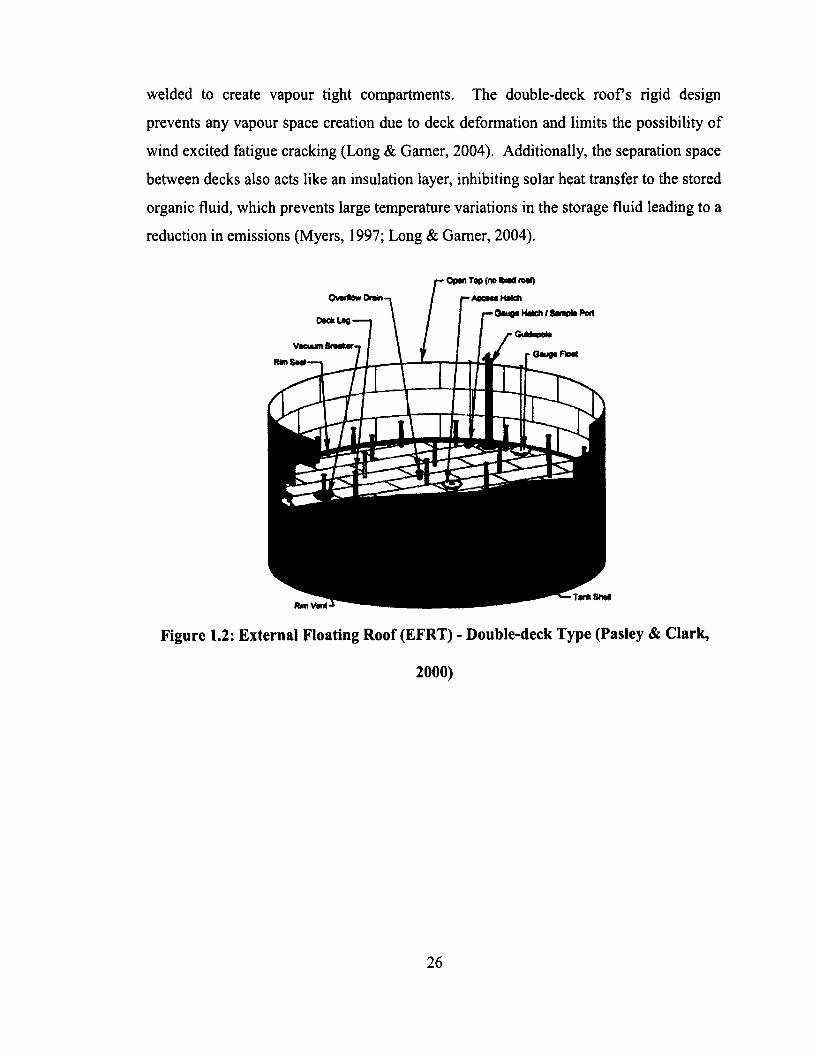
1.2.2.1 External Floating R oof Tank (EFRT)

An External Floating Roof Tank (EFRT) consists of an open-topped cylindrical steel

shell that surrounds a floating shell (roof). The floating roof is generally manufactured

from steel and rests on the liquid surface, rising and falling along with liquid level in the

tank. There are two widely implemented floating roof designs in these tanks: the pontoon

floating roof and the double-deck floating roof. Myers (1997) indicates that the pontoon

deck design, shown in Figure 1.3 is the most commonly used roof design used in tanks up

to about 65 metres in diameter. As described by Long & Gamer (2004), the roof can be

broken down into two main parts, the deck and outer annular pontoon. The deck is

generally manufactured from 3/16 inch steel plates that are seal welded on the weather

exposed side and stitch welded on the fluid exposed side. Depending on the fluid being

stored, crevice corrosion can be expected to occur on the lower surface, which can be

mitigated with seam welding. The outer annular pontoon ensures proper buoyancy and

provides the majority o f the structure’s rigidity. However, due to the inherent flexibility

of plate steel, the pontoon design is prone to the creation of vapour space at the center of

the roof and experiences fatigue cracking from wind excited deflections.

The double-deck design shown in Figure 1.3 is the heaviest and the most durable

of the external roof designs (due to its relatively high rigidity), and is the most

economical choice for smaller tanks (~10 metres) and very large tanks (60 to over 90

metres) (Myers, 1997). The roof is constructed from two seam welded decks that are

separated by a series o f circumferential and radial bulkheads. The bulkheads are seal

25

welded to create vapour tight compartments. The double-deck ro o fs rigid design

prevents any vapour space creation due to deck deformation and limits the possibility of

wind excited fatigue cracking (Long & Gamer, 2004). Additionally, the separation space

between decks also acts like an insulation layer, inhibiting solar heat transfer to the stored

organic fluid, which prevents large temperature variations in the storage fluid leading to a

reduction in emissions (Myers, 1997; Long & Gamer, 2004).

Opan Top (no «Md raei)

i—Accott Hatch

Figure 1.2: External Floating Roof (EFRT) - Double-deck Type (Pasley & Clark,

2000)

26

[v

Figure 1.3: External Floating Roof Tank (EFRT) - Pontoon Type Roof (EPA, 1995)

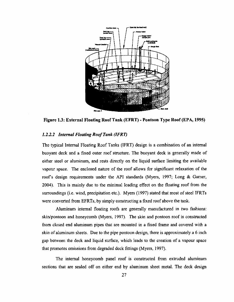
1.2.2.2 Internal Floating R oof Tank (IFRT)

The typical Internal Floating Roof Tanks (IFRT) design is a combination of an internal

buoyant deck and a fixed outer roof structure. The buoyant deck is generally made of

either steel or aluminum, and rests directly on the liquid surface limiting the available

vapour space. The enclosed nature of the roof allows for significant relaxation o f the

ro o fs design requirements under the API standards (Myers, 1997; Long & Gamer,

2004). This is mainly due to the minimal loading effect on the floating roof from the

surroundings (i.e. wind, precipitation etc.). Myers (1997) stated that most o f steel IFRTs

were converted from EFRTs, by simply constructing a fixed roof above the tank.

Aluminum internal floating roofs are generally manufactured in two fashions:

skin/pontoon and honeycomb (Myers, 1997). The skin and pontoon roof is constructed

from closed end aluminum pipes that are mounted in a fixed frame and covered with a

skin o f aluminum sheets. Due to the pipe pontoon design, there is approximately a 6 inch

gap between the deck and liquid surface, which leads to the creation o f a vapour space

that promotes emissions from degraded deck fittings (Myers, 1997).

The internal honeycomb panel roof is constructed from extruded aluminum

sections that are sealed off on either end by aluminum sheet metal. The deck design

27

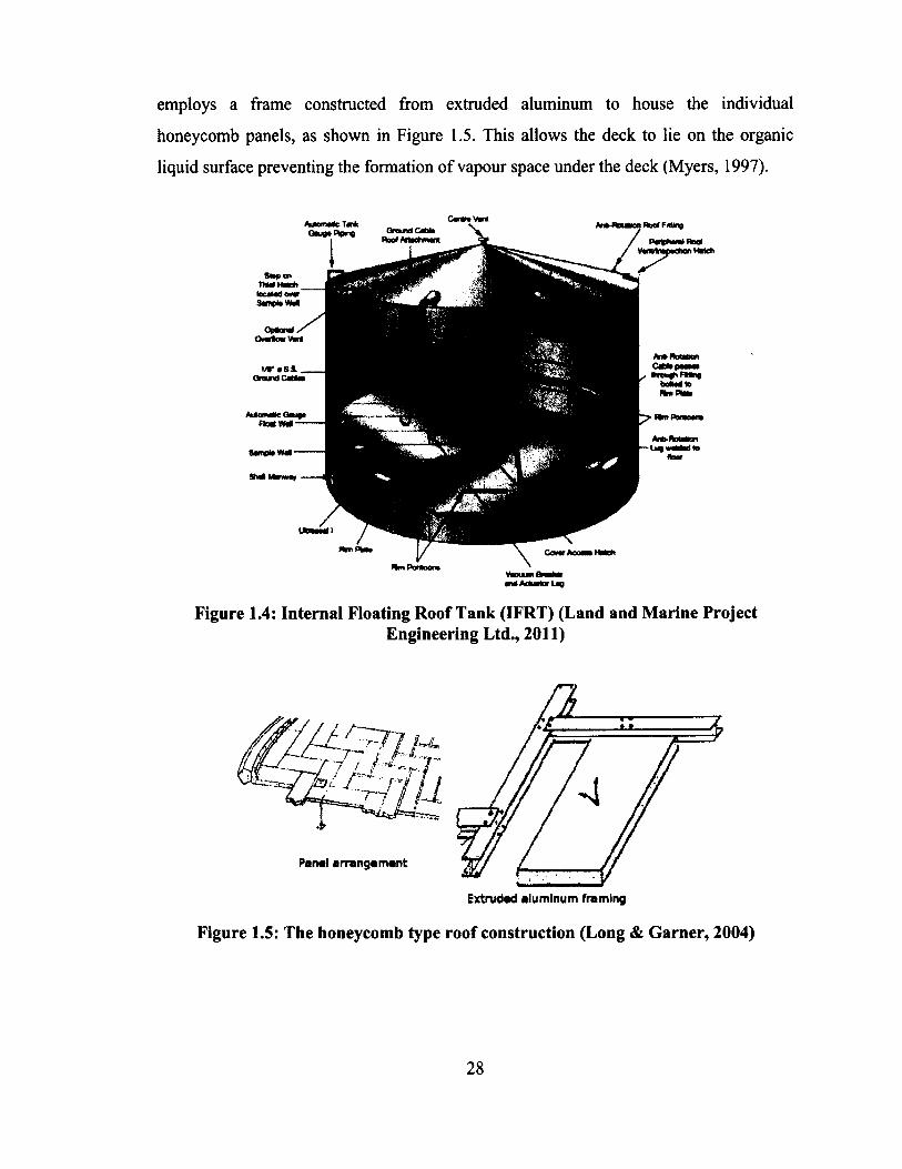
employs a frame constructed from extruded aluminum to house the individual

honeycomb panels, as shown in Figure 1.5. This allows the deck to lie on the organic

liquid surface preventing the formation o f vapour space under the deck (Myers, 1997).

end Actaalor lu g

Figure 1.4: Internal Floating Roof Tank (IFRT) (Land and Marine ProjectEngineering Ltd., 2011)

i L Q l U

Panel arrangem ent

Extruded aluminum framing

Figure 1.5: The honeycomb type roof construction (Long & Garner, 2004)

28

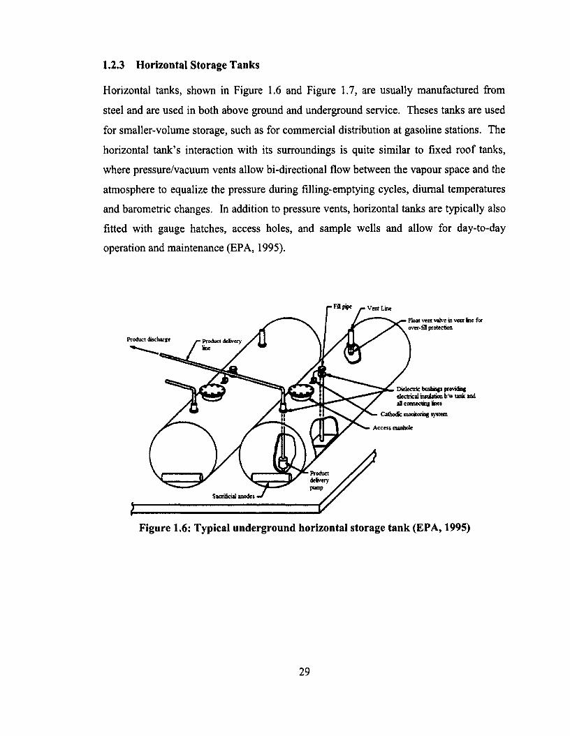
1.2.3 Horizontal Storage Tanks

Horizontal tanks, shown in Figure 1.6 and Figure 1.7, are usually manufactured from

steel and are used in both above ground and underground service. Theses tanks are used

for smaller-volume storage, such as for commercial distribution at gasoline stations. The

horizontal tank’s interaction with its surroundings is quite similar to fixed roof tanks,

where pressure/vacuum vents allow bi-directional flow between the vapour space and the

atmosphere to equalize the pressure during filling-emptying cycles, diurnal temperatures

and barometric changes. In addition to pressure vents, horizontal tanks are typically also

fitted with gauge hatches, access holes, and sample wells and allow for day-to-day

operation and maintenance (EPA, 1995).

Fill pipe * Vent Line

Product discharge Product deliveryline

Productdeliverypump

Sacrificial inodes

Float vent valve in vent Ine for over-fll protection

Dielectric bushings providing electrical insulation b'w tank and all connecting fines

Cafbodic monitoring system

Access manhole

Figure 1.6: Typical underground horizontal storage tank (EPA, 1995)

29

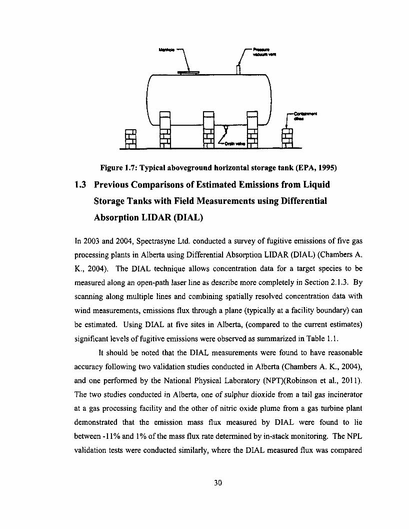
Figure 1.7: Typical aboveground horizontal storage tank (EPA, 1995)

1.3 Previous Comparisons of Estimated Emissions from Liquid

Storage Tanks with Field Measurements using Differential

Absorption LIDAR (DIAL)

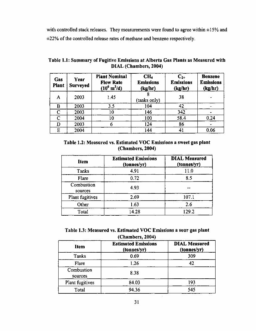
In 2003 and 2004, Spectrasyne Ltd. conducted a survey o f fugitive emissions o f five gas

processing plants in Alberta using Differential Absorption LIDAR (DIAL) (Chambers A.

K., 2004). The DIAL technique allows concentration data for a target species to be

measured along an open-path laser line as describe more completely in Section 2.1.3. By

scanning along multiple lines and combining spatially resolved concentration data with

wind measurements, emissions flux through a plane (typically at a facility boundary) can

be estimated. Using DIAL at five sites in Alberta, (compared to the current estimates)

significant levels of fugitive emissions were observed as summarized in Table 1.1.

It should be noted that the DIAL measurements were found to have reasonable

accuracy following two validation studies conducted in Alberta (Chambers A. K., 2004),

and one performed by the National Physical Laboratory (NPT)(Robinson et al., 2011).

The two studies conducted in Alberta, one o f sulphur dioxide from a tail gas incinerator

at a gas processing facility and the other o f nitric oxide plume from a gas turbine plant

demonstrated that the emission mass flux measured by DIAL were found to lie

between -11% and 1% of the mass flux rate determined by in-stack monitoring. The NPL

validation tests were conducted similarly, where the DIAL measured flux was compared

30

with controlled stack releases. They measurements were found to agree within ±15% and

±2 2 % of the controlled release rates o f methane and benzene respectively.

Table 1.1: Summary of Fugitive Emissions at Alberta Gas Plants as Measured withDIAL (Chambers, 2004)

GasPlant

YearSurveyed

Plant Nominal Flow Rate CIO6 m3/d)

c h 4Emissions

(kg/hr)

c2+Emissions

(kg/hr)

BenzeneEmissions

(kg/hr)

A 2003 1.45 8(tanks only) 38 -

B 2003 3.5 104 42 -

C 2003 10 146 342 -

C 2004 10 100 58.4 0.24D 2003 6 124 86 -

E 2004 144 41 0.06

Table 1.2: Measured vs. Estimated VOC Emissions a sweet gas plant(Chambers, 2004)

Item Estimated Emissions (tonnes/yr)

DIAL Measured (tonnes/yr)

Tanks 4.91 11.0Flare 0.72 8.5

Combustionsources 4.93 —

Plant fugitives 2.69 107.1Other 1.63 2.6Total 14.28 129.2

Table 1.3: Measured vs. Estimated VOC Emissions a sour gas plant(Chambers, 2004)

Item Estimated Emissions (tonnes/yr)

DIAL Measured (tonnes/yr)

Tanks 0.69 309Flare 1.26 42

Combustionsources 8.38

Plant fugitives 84.03 193Total 94.36 545

31

Measured fugitive emission rates obtained using DIAL were generally much

higher than predicted values using standard emission factor approaches, detailed in

Appendix B (Chambers, 2004). Table 1.2 and Table 1.3 show a direct comparison of

measured and estimated emission rates for specific plant components. For liquid storage

tanks specifically, DIAL measured emission rates were 2.2 and 450 times greater than

estimated emission rates (11.0 vs. 4.91 and 309 vs. 0.69 tonnes/yr respectively). More

generally, evaporative losses from liquid storage tanks contributed to about 36% methane

and 57% VOC of the total site emissions, notably one of the largest contributors to the

total plant emissions (Chambers, 2004). This trend has also been observed overseas by

experimental findings published by the IMPEL Network, where DIAL studies indicated

that -42% of the total VOCs released at an oil refinery were attributable to liquid storage

tanks (IMPEL Network, 2000).

While the DIAL studies did not present losses specific to the evaporative losses

from landed roofs, recent data published by the Texas Commission on Environmental

Quality (TCEQ) states the landing losses from tanks have been seriously under-reported,

amounting up to 7250 tons per year in the Houston-Galveston area alone (Schanbacher,

2007).

From the comparisons of the DIAL measurements to the current EPA estimates,

the need for further improvement in the estimation models can be seen; however, the

floating roof storage problem, due a significant number o f factors (wind speed, weather

degradation, etc.) is an immensely complex modeling problem. In addition, while DIAL

measurements indicate that the emissions are significantly higher than predicted, the tests

were necessarily conducted over a short periods o f time (relative to a full operating year),

and thereby cannot fully represent the evaporative loss distribution over the annual

operating period; due to the fact that there is no statistical basis for correlating annual

emissions from a single instance measurements. This argument, presented by Ferry

(Bosch Jr. & Logan, 2006), while holding merit in a statistical sense does not answer the

doubt of the EPA estimates presented by several snap-shot studies o f fugitive emissions

of storage tanks. It is from these opposing arguments, that the need for an economical

32

measurement system that can quantify the instantaneous emissions from liquid storage

tanks over the annual working period is required.

1.4 Experimental Objective

The goal o f this thesis was to design and develop a cost-effective measurement system

that uses Mid-IR absorption to measure the velocity of a transient hydrocarbon plume in a

lab-setting through cross correlative techniques. The proposed research is a stepping

stone to creating a real-time measurement system that uses a multi-line Mid-IR

absorption technology to measure in-field fugitive emissions mass flow rates from

storage tanks in a quantitative manner. This research will ultimately provide the

experimental findings that could be used to update the API correlations currently used by

industry. Having better models and diagnostics could reduce emissions by enabling

faster identification and repair of leaks and seals, improved operating procedures to

minimize activities associated with unintended emissions and better data from which to

justify economics o f more aggressive mitigation strategies (e.g. large scale vapour

recovery systems).

1.5 Organization of Thesis

The preceding discussion in Chapter 1 contains background information on liquid storage

tanks and their corresponding hydrocarbon evaporative losses. The official estimates for

liquid storage tanks are presented along with experimental findings from DIAL that

demonstrate their shortcomings and the need for monitoring technologies to improve the

accuracy of the estimates and allow for shorter leak detection timescales. In Chapter 2,

the background of various remote sensing techniques that implement absorption

spectroscopy to quantify background hydrocarbon concentrations in the atmosphere is

presented in the context of an economical in-field implementation. The latter half of the

chapter discusses motivation and selection of the technique to measure both the

concentration and velocity for the proposed in-lab VOC plume measurement sensor. In

Chapter 3, the background and theory o f the Mid-IR spectroscopic technique selected for

the VOC measurement sensor is presented. The theory of commercially available Mid-IR

spectroscopic components is presented along with the motivation and selection for the in

33

lab measurement sensor in the latter part of the chapter. Chapter 4 presents detailed

makeup of the two experimental setups used to benchmark the sensor and the selected

technique for a future full-scale VOC mass flux measurement sensor. Chapter 5 presents

the results and the overall performance o f the in-lab setup and the sensor’s concentration

sensitivity and associated uncertainty. The performance of the cross-correlative

technique is discussed in the latter part of Chapter 5. Finally, the conclusions o f this

research project and future work is presented in Chapter 6 .

34

Chapter 2

Remote Sensing of Evaporative Losses from

Liquid Storage Tanks

To the author’s knowledge, there are no specific direct measurement techniques available

for liquid storage tanks. However, there is a range o f different diagnostics that are

relevant. These are briefly reviewed here. In addition, qualitative techniques such as IR

camera surveying or downwind sampling can be utilized to detect or monitor emissions

without quantifying magnitudes (Chambers, 2004). While infrared cameras offer a fast

technique to detect leaks, they are labour intensive and are adversely affected by complex

backgrounds, lighting conditions and their own inherent detection limits. Because these

approaches are non-quantitative they are not considered further.

2.1 Absorption Spectroscopy

Absorption spectroscopy uses measured absorption o f electromagnetic radiation passing

through a sample to calculate mean concentration o f a target species along the optical

path. Every molecule exhibits its own absorption spectrum which is based on the

quantum mechanical change induced by the absorbed electromagnetic radiation. Spectral

absorption strength data as a function of optical frequency, temperature, and pressure are

available for many different molecules in databases such as HITRAN (2008). The

absorption o f infrared (IR) electromagnetic energy by molecules is restricted to the

energy changes between the rotational and vibrational (ro-vibration) quantum states. If

the frequency o f the incoming electromagnetic radiation matches the ro-vibrational

frequency of the target molecule, the electromagnetic energy will be absorbed (So et al.

2009). By measuring the intensity o f the radiation before and after passing through the

35

test sample, the absorption spectrum can be experimentally ascertained. The spectral

region with the highest absorbance values defines the Optimal Spectral Region (OSR),

which for a given molecule can be targeted to measure the concentration o f the molecule

with high accuracy (Hollas, 2004). The following sections briefly describe various types

o f absorption spectroscopy that have the capacity to be implemented in the field

2.1.1 Direct Absorption Spectroscopy (DAS)

Direct Absorption Spectroscopy (DAS) is one o f the simpler implementations of

absorption spectroscopy. There are two main types o f DAS: monochromatic DAS and

scanned-wavelength DAS. Monochromatic DAS uses a fixed-wavelength source to

probe a single spectral absorption peak. Scanned-wavelength DAS is generally

accomplished using a Tunable Diode Laser (TDL), which allows for rapid scanning of

the optical wavelength across an absorption feature to obtain both baseline and peak

intensity measurements that are proportional to the concentration o f the target gas. The

wavelength scan is achieved by varying the injection current to the laser diode. Scanned-

wavelength DAS permits discrimination of the target gas from background absorption

from other species (such a dust particulates). However, DAS is highly susceptible to

noise introduced through the laser sources and/or the optical system. In general,

reference detectors are utilized to measure the laser’s power before absorption by the

target gas to establish a proper base datum (which can drift over time). The use o f a

reference detector also enables removal o f excess laser noise from the measured signals

(Rieker, 2009).

2.1.2 Wavelength-Modulation Spectroscopy (WMS)

Wavelength Modulation Spectroscopy (WMS) is similar to scanned-wavelength DAS

where the absorption feature of the target gas is scanned across a (wavelength)

bandwidth; however, WMS superimposes a secondary high modulation frequency, low

amplitude sinusoid signal in addition to the (relatively) slower ramp signal. The

interaction between a rapidly alternating wavelength and a nonlinear absorption feature

creates a series o f nth order harmonics o f the absorption feature at periods of the

modulation frequency (Svensson et al., 2008). By measuring the 2nd order harmonic, it is

36

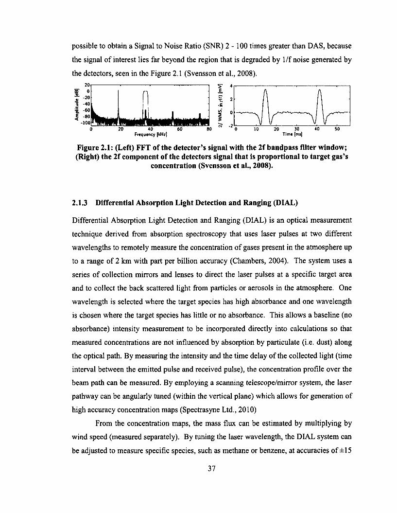
possible to obtain a Signal to Noise Ratio (SNR) 2 - 1 0 0 times greater than DAS, because

the signal of interest lies far beyond the region that is degraded by 1 /f noise generated by

the detectors, seen in the Figure 2.1 (Svensson et al., 2008).

Figure 2.1: (Left) FFT of the detector’s signal with the 2f bandpass filter window;(Right) the 2f component of the detectors signal that is proportional to target gas’s

concentration (Svensson et al., 2008).

2.1.3 Differential Absorption Light Detection and Ranging (DIAL)

Differential Absorption Light Detection and Ranging (DIAL) is an optical measurement

technique derived from absorption spectroscopy that uses laser pulses at two different

wavelengths to remotely measure the concentration of gases present in the atmosphere up

to a range o f 2 km with part per billion accuracy (Chambers, 2004). The system uses a

series o f collection mirrors and lenses to direct the laser pulses at a specific target area

and to collect the back scattered light from particles or aerosols in the atmosphere. One

wavelength is selected where the target species has high absorbance and one wavelength

is chosen where the target species has little or no absorbance. This allows a baseline (no

absorbance) intensity measurement to be incorporated directly into calculations so that

measured concentrations are not influenced by absorption by particulate (i.e. dust) along

the optical path. By measuring the intensity and the time delay of the collected light (time

interval between the emitted pulse and received pulse), the concentration profile over the

beam path can be measured. By employing a scanning telescope/mirror system, the laser

pathway can be angularly tuned (within the vertical plane) which allows for generation of

high accuracy concentration maps (Spectrasyne Ltd., 2010)

From the concentration maps, the mass flux can be estimated by multiplying by

wind speed (measured separately). By tuning the laser wavelength, the DIAL system can

be adjusted to measure specific species, such as methane or benzene, at accuracies o f ±15

201------------------.------------------.------------------.------------------ j r 40 /~\ JL

:L J L , „ll L..40

Frequency [kHz]20 30 40 50

Time [mi)

37

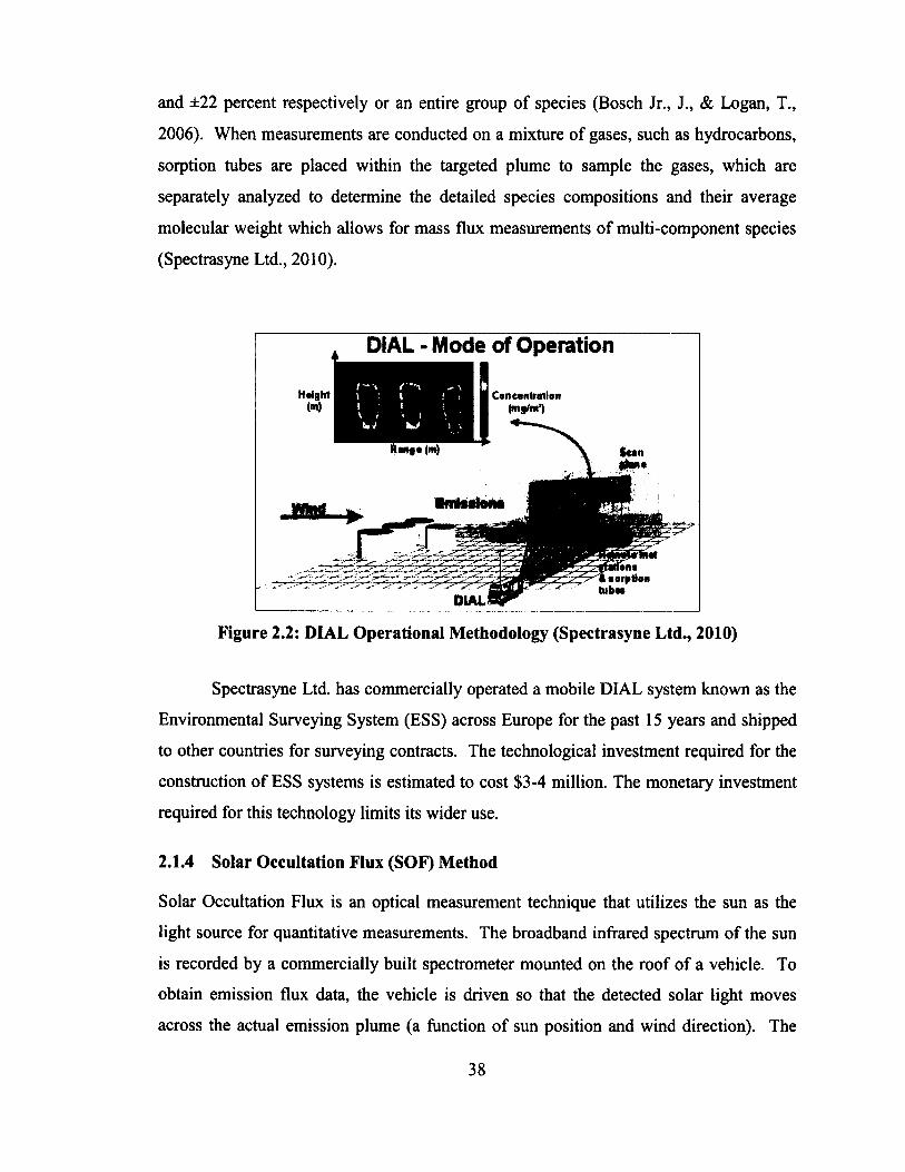
and ±22 percent respectively or an entire group of species (Bosch Jr., J., & Logan, T.,

2006). When measurements are conducted on a mixture of gases, such as hydrocarbons,

sorption tubes are placed within the targeted plume to sample the gases, which are

separately analyzed to determine the detailed species compositions and their average

molecular weight which allows for mass flux measurements o f multi-component species

(Spectrasyne Ltd., 2010).

Figure 2.2: DIAL Operational Methodology (Spectrasyne Ltd., 2010)

Spectrasyne Ltd. has commercially operated a mobile DIAL system known as the

Environmental Surveying System (ESS) across Europe for the past 15 years and shipped

to other countries for surveying contracts. The technological investment required for the

construction of ESS systems is estimated to cost $3-4 million. The monetary investment

required for this technology limits its wider use.

2.1.4 Solar Occultation Flux (SOF) Method

Solar Occultation Flux is an optical measurement technique that utilizes the sun as the

light source for quantitative measurements. The broadband infrared spectrum of the sun

is recorded by a commercially built spectrometer mounted on the roof o f a vehicle. To

obtain emission flux data, the vehicle is driven so that the detected solar light moves

across the actual emission plume (a function of sun position and wind direction). The

DIAL - Mode of Operation

H W f • (mj

sorp tiontubas

Haight(m)

Concentration(mg/m*)

38

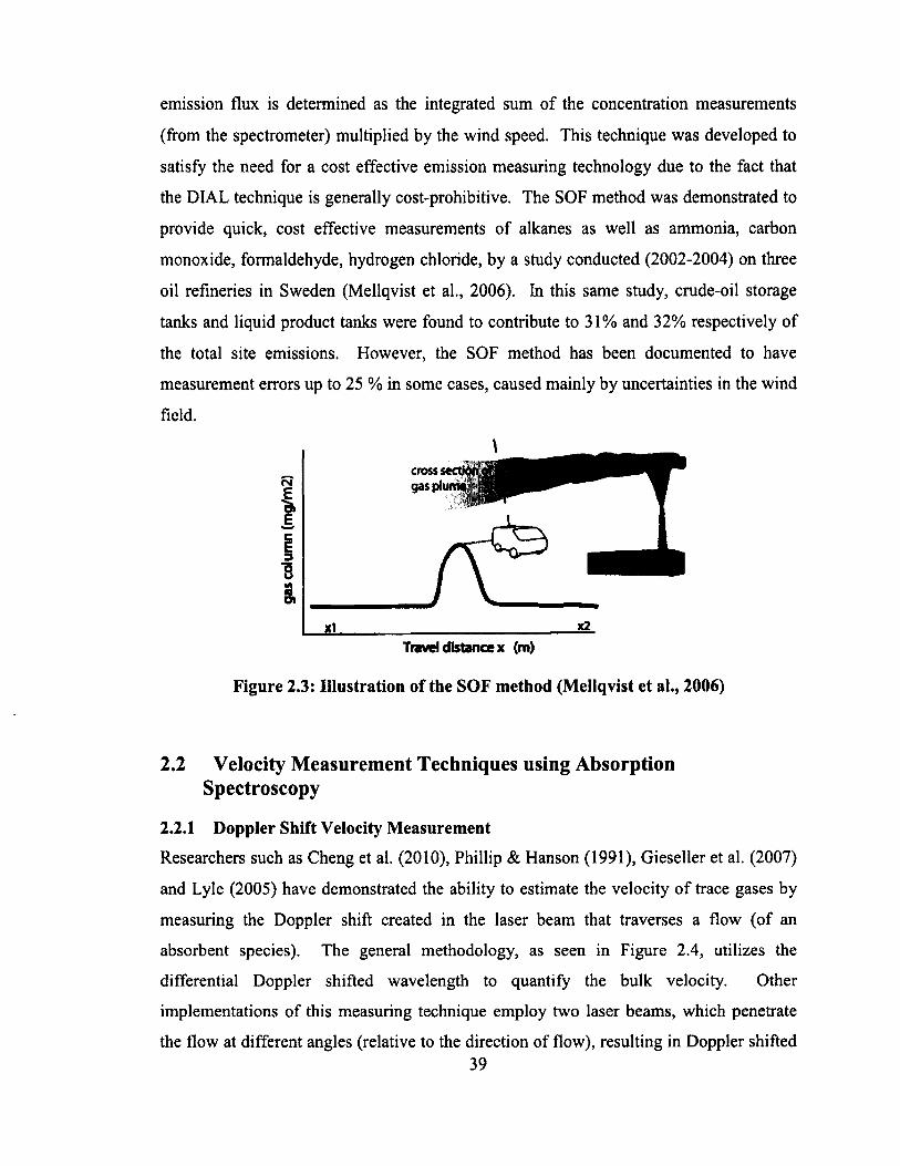
emission flux is determined as the integrated sum of the concentration measurements

(from the spectrometer) multiplied by the wind speed. This technique was developed to

satisfy the need for a cost effective emission measuring technology due to the fact that

the DIAL technique is generally cost-prohibitive. The SOF method was demonstrated to

provide quick, cost effective measurements of alkanes as well as ammonia, carbon

monoxide, formaldehyde, hydrogen chloride, by a study conducted (2002-2004) on three

oil refineries in Sweden (Mellqvist et al., 2006). In this same study, crude-oil storage

tanks and liquid product tanks were found to contribute to 31% and 32% respectively of

the total site emissions. However, the SOF method has been documented to have

measurement errors up to 25 % in some cases, caused mainly by uncertainties in the wind

field.

\cross s*coo gaspturwi

il---------------------------------------------—Travel distance x (m)

Figure 2.3: Illustration of the SOF method (Mellqvist et al., 2006)

2.2 Velocity Measurement Techniques using Absorption Spectroscopy

2.2.1 Doppler Shift Velocity Measurement

Researchers such as Cheng et al. (2010), Phillip & Hanson (1991), Gieseller et al. (2007)

and Lyle (2005) have demonstrated the ability to estimate the velocity o f trace gases by

measuring the Doppler shift created in the laser beam that traverses a flow (of an

absorbent species). The general methodology, as seen in Figure 2.4, utilizes the

differential Doppler shifted wavelength to quantify the bulk velocity. Other

implementations o f this measuring technique employ two laser beams, which penetrate

the flow at different angles (relative to the direction of flow), resulting in Doppler shifted39

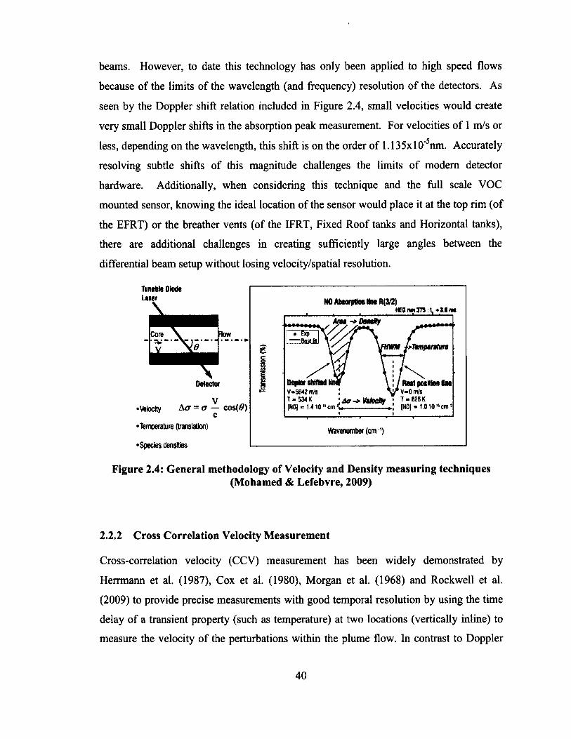
beams. However, to date this technology has only been applied to high speed flows

because o f the limits o f the wavelength (and frequency) resolution o f the detectors. As

seen by the Doppler shift relation included in Figure 2.4, small velocities would create

very small Doppler shifts in the absorption peak measurement. For velocities of 1 m/s or

less, depending on the wavelength, this shift is on the order of 1.135xl0'5nm. Accurately

resolving subtle shifts o f this magnitude challenges the limits of modem detector

hardware. Additionally, when considering this technique and the full scale VOC

mounted sensor, knowing the ideal location o f the sensor would place it at the top rim (of

the EFRT) or the breather vents (of the IFRT, Fixed Roof tanks and Horizontal tanks),

there are additional challenges in creating sufficiently large angles between the

differential beam setup without losing velocity/spatial resolution.

TunaUs Diode Laser

Core Row • Exp — Best SI

v £

•Velocity

•Temperature (translation)

•Species densities

A a ~ a — cos(9) c

NO Absorption Hne R(3/2)HE8wn37VI.-H.SiM

Ant ->DtatHy

Tmptntm

Dopier shittedV-5642 m<sT-534K 'Aa-> VltOCily(NO) - 1.410 M cm ’L_________ -

Rest position HneV«0nVs T - 826 K (NO) = 1.010,s cm3

Wavenumber ( c m ')

Figure 2.4: General methodology of Velocity and Density measuring techniques(Mohamed & Lefebvre, 2009)

2.2.2 Cross Correlation Velocity Measurement

Cross-correlation velocity (CCV) measurement has been widely demonstrated by

Herrmann et al. (1987), Cox et al. (1980), Morgan et al. (1968) and Rockwell et al.

(2009) to provide precise measurements with good temporal resolution by using the time

delay of a transient property (such as temperature) at two locations (vertically inline) to

measure the velocity of the perturbations within the plume flow. In contrast to Doppler

40

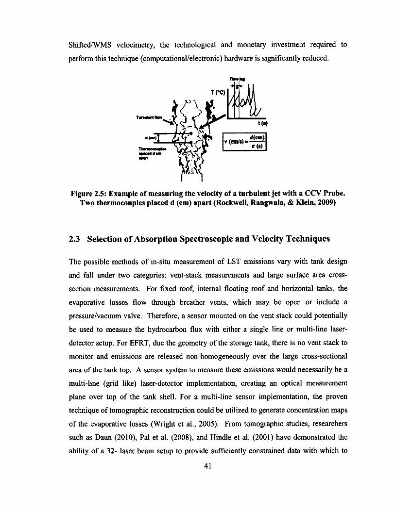
Shifted/WMS velocimetry, the technological and monetary investment required to

perform this technique (computational/electronic) hardware is significantly reduced.

Tlnwlaf

T (*C)

t(»)

rf(cm )v(cm/t)

r(»)4cm

Figure 2.5: Example of measuring the velocity of a turbulent jet with a CCV Probe.Two thermocouples placed d (cm) apart (Rockwell, Rangwala, & Klein, 2009)

2.3 Selection of Absorption Spectroscopic and Velocity Techniques

The possible methods o f in-situ measurement o f LST emissions vary with tank design

and fall under two categories: vent-stack measurements and large surface area cross-

section measurements. For fixed roof, internal floating roof and horizontal tanks, the

evaporative losses flow through breather vents, which may be open or include a

pressure/vacuum valve. Therefore, a sensor mounted on the vent stack could potentially

be used to measure the hydrocarbon flux with either a single line or multi-line laser-

detector setup. For EFRT, due the geometry o f the storage tank, there is no vent stack to

monitor and emissions are released non-homogeneously over the large cross-sectional

area o f the tank top. A sensor system to measure these emissions would necessarily be a

multi-line (grid like) laser-detector implementation, creating an optical measurement

plane over top of the tank shell. For a multi-line sensor implementation, the proven

technique o f tomographic reconstruction could be utilized to generate concentration maps

o f the evaporative losses (Wright et al., 2005). From tomographic studies, researchers

such as Daun (2010), Pal et al. (2008), and Hindle et al. (2001) have demonstrated the

ability o f a 32- laser beam setup to provide sufficiently constrained data with which to

41

reconstruct the spatially resolved concentration o f the absorbing species. However, these

studies were performed over relatively small control space (on the order o f 50-84

millimetres) where the spatial resolution is documented to be inversely proportionally to

the number o f beams. This implies that a fixture full scale sensor would require a

significant number o f laser-detector pairs to provide reasonable spatial resolution above

the EFRT. To satisfy these design criteria, DAS appears to be the most economical

viable technique of the presented spectroscopic techniques. Considering the sizable

monetary investment (-$50000 and up) required for a laser-detector pair that utilizes

WMS (required for Doppler shift velocimetry) with reasonable sensitivity, the economic

feasibility o f utilizing the Doppler shift technique is very poor for the single line setup let

a alone the multi-line setup required for EFRTs.

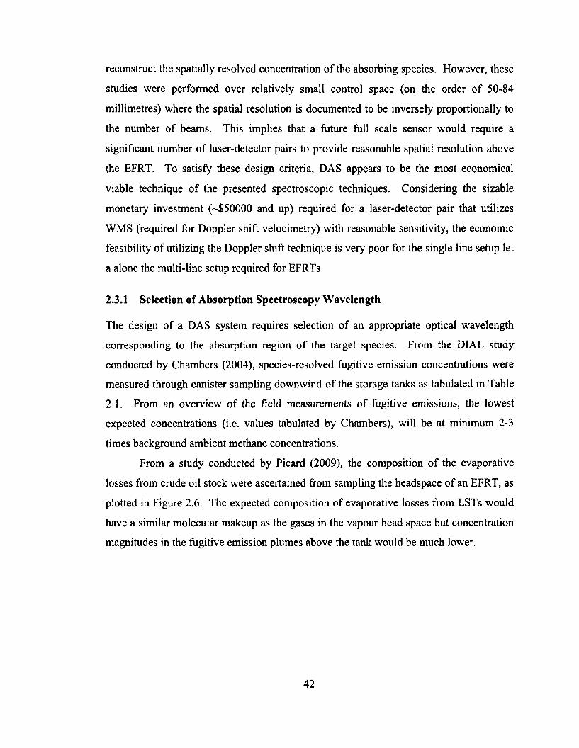
2.3.1 Selection of Absorption Spectroscopy Wavelength

The design of a DAS system requires selection o f an appropriate optical wavelength

corresponding to the absorption region o f the target species. From the DIAL study

conducted by Chambers (2004), species-resolved fugitive emission concentrations were

measured through canister sampling downwind o f the storage tanks as tabulated in Table

2.1. From an overview o f the field measurements o f fugitive emissions, the lowest

expected concentrations (i.e. values tabulated by Chambers), will be at minimum 2-3

times background ambient methane concentrations.

From a study conducted by Picard (2009), the composition o f the evaporative

losses from crude oil stock were ascertained from sampling the headspace o f an EFRT, as

plotted in Figure 2.6. The expected composition of evaporative losses from LSTs would

have a similar molecular makeup as the gases in the vapour head space but concentration

magnitudes in the fugitive emission plumes above the tank would be much lower.

42

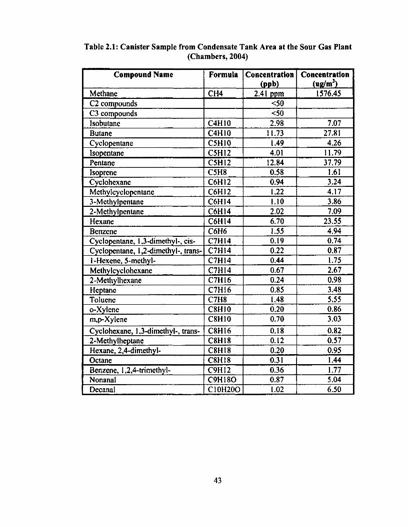
Table 2.1: Canister Sample from Condensate Tank Area at the Sour Gas Plant(Chambers, 2004)

Compound Name Formula Concentration(ppb)

Concentration(ug/m3)

Methane CH4 2.41 ppm 1576.45C2 compounds <50C3 compounds <50Isobutane C4H10 2.98 7.07Butane C4H10 11.73 27.81Cyclopentane C5H10 1.49 4.26Isopentane C5H12 4.01 11.79Pentane C5H12 12.84 37.79Isoprene C5H8 0.58 1.61Cyclohexane C6H12 0.94 3.24Mcthylcyclopentanc C6H12 1.22 4.173-Methylpentane C6H14 1.10 3.862-Methylpentane C6H14 2.02 7.09Hexane C6H14 6.70 23.55Benzene C6H6 1.55 4.94Cyclopentane, 1,3-dimethyl-, cis- C7H14 0.19 0.74Cyclopentane, 1,2-dimethyl-, trans- C7H14 0.22 0.871-Hexene, 5-methyl- C7H14 0.44 1.75Methylcyclohexane C7H14 0.67 2.672-Methylhexane C7H16 0.24 0.98Heptane C7H16 0.85 3.48Toluene C7H8 1.48 5.55o-Xylcne C8H10 0.20 0.86m,p-Xylene C8H10 0.70 3.03Cyclohexane, 1,3-dimethyl-, trans- C8H16 0.18 0.822-Methylheptane C8H18 0.12 0.57Hexane, 2,4-dimethyl- C8H18 0.20 0.95Octane C8H18 0.31 1.44Benzene, 1,2,4-trimethyl- C9H12 0.36 1.77Nonanal C9H180 0.87 5.04Decanal C10H20O 1.02 6.50

43

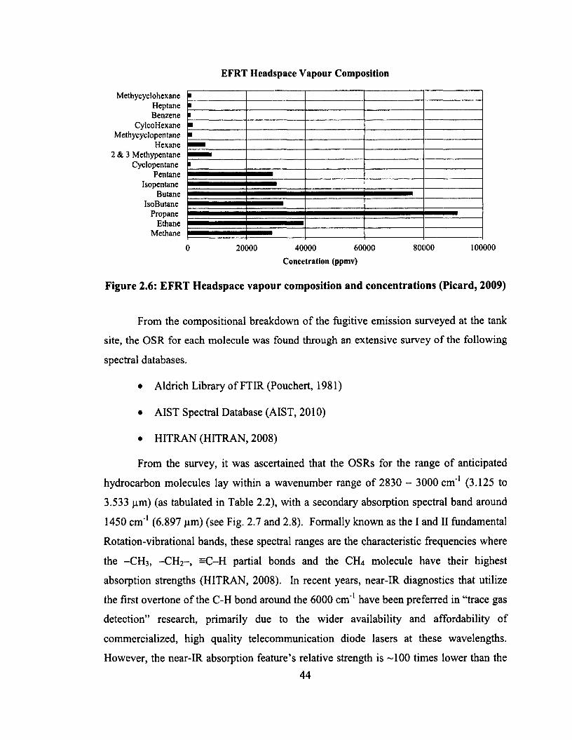
EFRT Headspace Vapour Composition

Methycyclohexane Heptane Benzene

CylcoHexane Methycyclopentane

Hexane 2 & 3 Methypentane

Cyclopentane Pentane

Isopentane Butane

IsoButane Propane

Ethane Methane

0 20000 40000 60000 80000 100000

Concetration (ppmv)

Figure 2.6: EFRT Headspace vapour composition and concentrations (Picard, 2009)

From the compositional breakdown o f the fugitive emission surveyed at the tank

site, the OSR for each molecule was found through an extensive survey o f the following

spectral databases.

• Aldrich Library o f FTIR (Pouchert, 1981)

• AIST Spectral Database (AIST, 2010)

• HITRAN (HITRAN, 2008)

From the survey, it was ascertained that the OSRs for the range of anticipated

hydrocarbon molecules lay within a wavenumber range o f 2830 - 3000 cm ' 1 (3.125 to

3.533 pm) (as tabulated in Table 2.2), with a secondary absorption spectral band around

1450 cm ' 1 (6.897 pm) (see Fig. 2.7 and 2.8). Formally known as the I and II fundamental

Rotation-vibrational bands, these spectral ranges are the characteristic frequencies where

the -CH3, -C H 2-, =C-H partial bonds and the CH4 molecule have their highest

absorption strengths (HITRAN, 2008). In recent years, near-IR diagnostics that utilize

the first overtone o f the C-H bond around the 6000 cm ' 1 have been preferred in “trace gas

detection” research, primarily due to the wider availability and affordability of

commercialized, high quality telecommunication diode lasers at these wavelengths.

However, the near-IR absorption feature’s relative strength is ~ 100 times lower than the

44

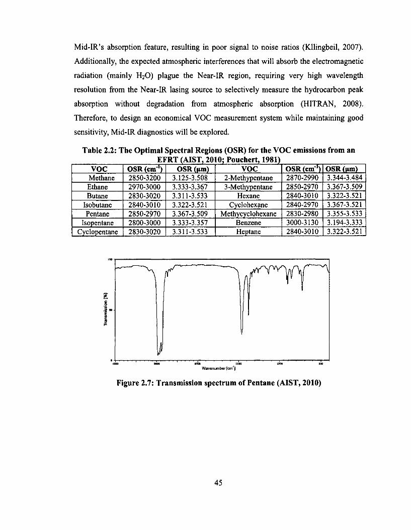
Mid-IR’s absorption feature, resulting in poor signal to noise ratios (Kllingbeil, 2007).

Additionally, the expected atmospheric interferences that will absorb the electromagnetic

radiation (mainly H2 O) plague the Near-IR region, requiring very high wavelength

resolution from the Near-IR lasing source to selectively measure the hydrocarbon peak

absorption without degradation from atmospheric absorption (HITRAN, 2008).

Therefore, to design an economical VOC measurement system while maintaining good

sensitivity, Mid-IR diagnostics will be explored.

Table 2.2: The Optimal Spectral Regions (OSR) for the VOC emissions from anEFRT (AIST, 201 0; Pouchert, 1981)

VOC OSR (cm1) OSR (i»m) VOC OSR (cm1) OSR (um)Methane 2850-3200 3.125-3.508 2-Methypentane 2870-2990 3.344-3.484Ethane 2970-3000 3.333-3.367 3-Methypentane 2850-2970 3.367-3.509Butane 2830-3020 3.311-3.533 Hexane 2840-3010 3.322-3.521

Isobutane 2840-3010 3.322-3.521 Cyclohexane 2840-2970 3.367-3.521Pentane 2850-2970 3.367-3.509 Methycyclohexane 2830-2980 3.355-3.533

Isopentane 2800-3000 3.333-3.357 Benzene 3000-3130 3.194-3.333Cyclopentane 2830-3020 3.311-3.533 Heptane 2840-3010 3.322-3.521

Wavanumber [cm1]

Figure 2.7: Transmission spectrum of Pentane (AIST, 2010)

45

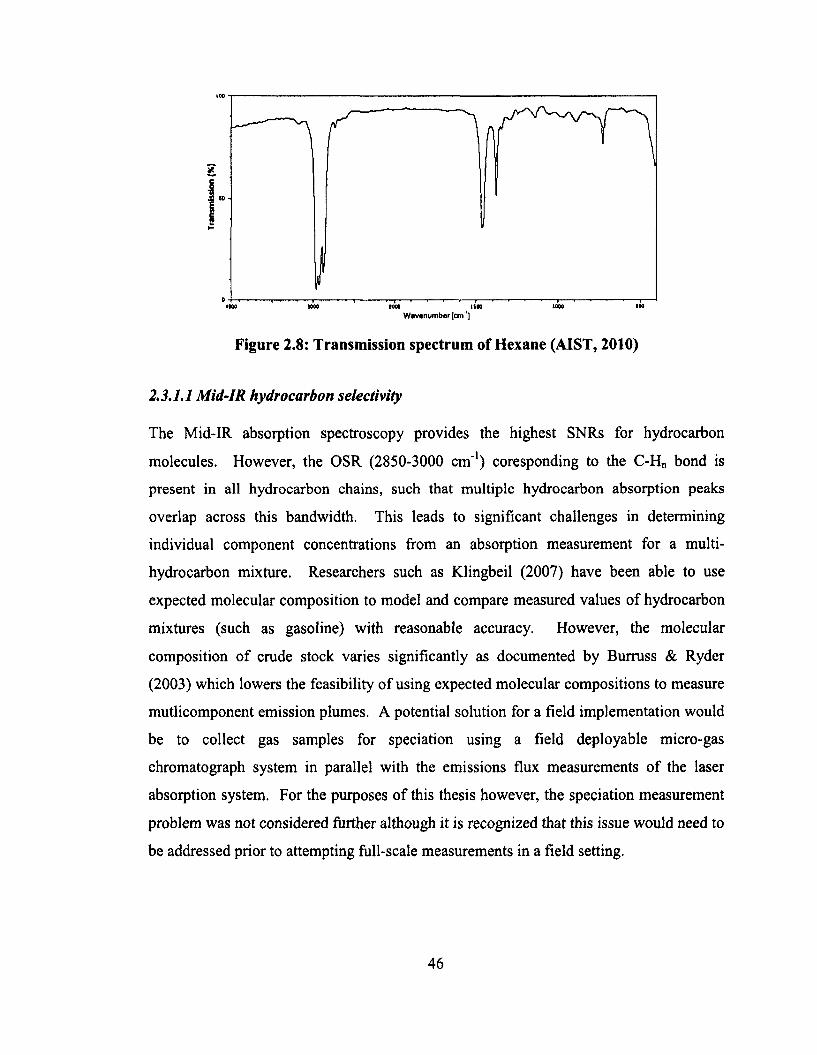
1

I

Wavenumber [cm']

Figure 2.8: Transmission spectrum of Hexane (AIST, 2010)

2.3.1.1 Mid-IR hydrocarbon selectivity

The Mid-IR absorption spectroscopy provides the highest SNRs for hydrocarbon

molecules. However, the OSR (2850-3000 cm '1) coresponding to the C-Hn bond is

present in all hydrocarbon chains, such that multiple hydrocarbon absorption peaks

overlap across this bandwidth. This leads to significant challenges in determining

individual component concentrations from an absorption measurement for a multi

hydrocarbon mixture. Researchers such as Klingbeil (2007) have been able to use

expected molecular composition to model and compare measured values of hydrocarbon

mixtures (such as gasoline) with reasonable accuracy. However, the molecular

composition o f crude stock varies significantly as documented by Burruss & Ryder

(2003) which lowers the feasibility of using expected molecular compositions to measure

mutlicomponent emission plumes. A potential solution for a field implementation would

be to collect gas samples for speciation using a field deployable micro-gas

chromatograph system in parallel with the emissions flux measurements of the laser

absorption system. For the purposes of this thesis however, the speciation measurement

problem was not considered further although it is recognized that this issue would need to

be addressed prior to attempting full-scale measurements in a field setting.

46

Chapter 3

Background on MID-IR Absorption

Spectroscopy and Technology

3.1 Mid-IR Absorption Spectroscopy

The Beer-Lambert law relates the absorption of electromagnetic radiation (at a known

frequency) to the concentration of the species along the optical path as shown in Eq. 3.1

(Hollas, 2004),

a = — Inj - = —/n(r R) = a (T ,P ,v ) * C * L (3.1)*0

where:T/j is the transmittance o f the target gas [-],

a is the absorbance of the target gas [-],

/ 0 is the power o f the incident radiation [W],

/ is the power of the transmitted radiation [W],

o(T, P, v) is the molar absorption coefficient as a function temperature, pressure

and wavelength [m2 /mol],

C is the molar concentration of the target gas [mol/ m3],

L is the path length through the target gas traversed by the electromagnetic

radiation [m],

P is the barometric pressure [Pa]

v is the wavelength [m], and

T is the temperature o f the gas mixture [K].

47

The Beer-Lambert law can be modified to measure the absorption o f multi-component

gases; the individual contributions are linearly cumulative as seen in Eq. 3.2 (Hollas,

2004; Kllingbeil, 2007).

amix = - l n j - = - l n ( j Rm.x) = P , v ) * Q * L (3.2)

where:

TRmix *s transmittance o f the multi-component gas mixture [-],

a mix is the absorbance measured o f the multi-component gas mixture [-],

<Ti(T, P , v ) is molar absorption coefficient o f the ith gas as a function temperature,

pressure and wavelength [m2 /mol], and

Ci is the molar concentration o f the o f the ith gas [mol/ m3].

The molar absorption coefficient varies with changes in gas sample temperature,

barometric pressure, and the wavelength o f electromagnetic radiation. While a change in

pressure affects the peak strength of the molar absorption coefficient, the low variability

of ambient pressure means that drastic changes to the molar absorption coefficient are not

expected. Therefore, it is feasible to determine concentration by measuring the ambient

pressure and directly interpolating between expected molar absorption constants

calculated at different pressures (Hollas, 2004; D ’Amato, 2006).

Figure 3.1 and Figure 3.2 show mid-IR absorption spectrum o f methane near the

target OSR (3.392pm) selected for the VOC sensor as a function o f temperature and

pressure.

48

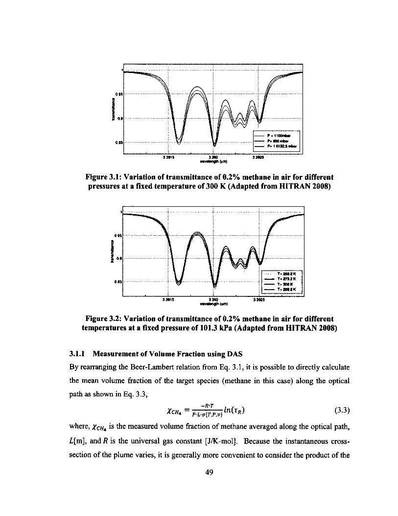
0.95

5 o.0

0 85

33025

Figure 3.1: Variation of transmittance of 0.2% methane in air for different pressures at a fixed temperature of 300 K (Adapted from HITRAN 2008)

005

00

085

33015 ' 3302 ' 33025tMMfengtfi (pm)

Figure 3.2: Variation of transmittance of 0.2% methane in air for different temperatures at a fixed pressure of 101.3 kPa (Adapted from HITRAN 2008)

3.1.1 Measurement of Volume Fraction using DAS

By rearranging the Beer-Lambert relation from Eq. 3.1, it is possible to directly calculate

the mean volume fraction of the target species (methane in this case) along the optical

path as shown in Eq. 3.3,

= f ' t' A f j . . - ) ln (T |i) <3-3)

where, Xch4 is the measured volume fraction o f methane averaged along the optical path,

L[m], and R is the universal gas constant [J/K-mol]. Because the instantaneous cross-

section o f the plume varies, it is generally more convenient to consider the product o f the

49

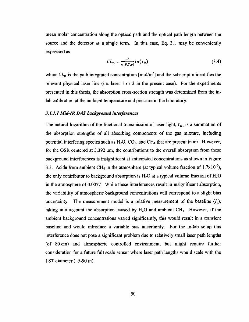
mean molar concentration along the optical path and the optical path length between the

source and the detector as a single term. In this case, Eq. 3.1 may be conveniently

expressed as

<3 '4>

where CLn is the path integrated concentration [mol/m2] and the subscript n identifies the

relevant physical laser line (i.e. laser 1 or 2 in the present case). For the experiments

presented in this thesis, the absorption cross-section strength was determined from the in

lab calibration at the ambient temperature and pressure in the laboratory.

3.1.1.1 Mid-IR DAS background interferences

The natural logarithm of the fractional transmission of laser light, rR, is a summation of

the absorption strengths o f all absorbing components o f the gas mixture, including

potential interfering species such as H2 O, CO2 , and CH4 that are present in air. However,

for the OSR centered at 3.392 pm, the contributions to the overall absorption from these

background interferences is insignificant at anticipated concentrations as shown in Figure

3.3. Aside from ambient CH4 in the atmosphere (at typical volume fraction o f 1.7xl0'6),

the only contributor to background absorption is H2 O at a typical volume fraction o f H2 O

in the atmosphere of 0.0077. While these interferences result in insignificant absorption,

the variability of atmospheric background concentrations will correspond to a slight bias

uncertainty. The measurement model is a relative measurement o f the baseline (70),

taking into account the absorption caused by H2 O and ambient CH4 . However, if the

ambient background concentrations varied significantly, this would result in a transient

baseline and would introduce a variable bias uncertainty. For the in-lab setup this

interference does not pose a significant problem due to relatively small laser path lengths

(of 80 cm) and atmospheric controlled environment, but might require further

consideration for a future full scale sensor where laser path lengths would scale with the

LST diameter (-5-90 m).

50

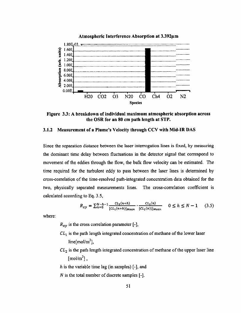
Atmospheric Interference Absorption at 3.392pm

1.80E-03 3 1.60E-03 § 1.40E-03 £ 1.20E-03 ", 1.00E-03 § 8.00E-04 '§, 6.00E-04 S 4.00E-04 < 2.00E-04

0.00E+00 — iH20 C 02 03 N20 CO Ch4 0 2 N2

Species

Figure 3.3: A breakdown of individual maximum atmospheric absorption across the OSR for an 80 cm path length at STP.

3.1.2 Measurement of a Plume’s Velocity through CCV with Mid-IR DAS

Since the separation distance between the laser interrogation lines is fixed, by measuring

the dominant time delay between fluctuations in the detector signal that correspond to

movement o f the eddies through the flow, the bulk flow velocity can be estimated. The

time required for the turbulent eddy to pass between the laser lines is determined by

cross-correlation o f the time-resolved path-integrated concentration data obtained for the

two, physically separated measurements lines. The cross-correlation coefficient is

calculated according to Eq. 3.5,

O — y N - h - l CL1(n+h) ' CL2(n) t) < h < N — 1 H S3R x y - L n = 0 (c i l(n+/i)]jifefln [CL2(n)))Mean ° - h ~ N

where:

Rxy is the cross correlation parameter [-],

CL1 is the path length integrated concentration o f methane o f the lower laser

line[mol/m2],

CL2 is the path length integrated concentration o f methane o f the upper laser line

[mol/m2] ,

h is the variable time lag (in samples) [-], and

N is the total number of discrete samples [-].

51

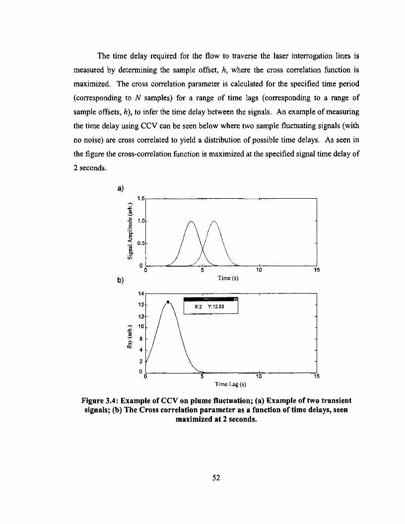
The time delay required for the flow to traverse the laser interrogation lines is

measured by determining the sample offset, h, where the cross correlation function is

maximized. The cross correlation parameter is calculated for the specified time period

(corresponding to N samples) for a range of time lags (corresponding to a range of

sample offsets, h), to infer the time delay between the signals. An example of measuring

the time delay using CCV can be seen below where two sample fluctuating signals (with

no noise) are cross correlated to yield a distribution o f possible time delays. As seen in

the figure the cross-correlation function is maximized at the specified signal time delay of

2 seconds.

a)

O.

0.5

Time (s)b)

X:2 Y:12.53

Time Lag (s)

Figure 3.4: Example of CCV on plume fluctuation; (a) Example of two transient signals; (b) The Cross correlation parameter as a function of time delays, seen

maximized at 2 seconds.

52

The main parameters that affect the cross correlation function are the sampling

frequency, sampling period, turbulent eddy behaviour, laser beam separation,

measurement noise and the measurement signal’s correlative properties (Rockwell et al.

2009). The sampling frequency determines the minimum turbulent fluctuation that can

be resolved. In practice, the maximum sampling frequency is limited by the detector

response time. To ensure proper transient resolution (i.e. no distortion due to low sample

rates), a high sampling frequency is required, but the improvement in accuracy

exponentially decays beyond a critical sampling frequency. The critical frequency is

determined by the dynamics o f the plume flow and the transient response o f the detector.

The sampling period must be long enough to identify a lag, but short enough so that the

sensor can provide velocity readings at a reasonable rate. The turbulent eddy-size and the

beam separation determine the sensor’s ability to capture a time delay from a transient

flow. For example, if the plume’s eddy dissipation/generation is high and the beam

spacing is relatively large, then the accuracy of the correlation function is reduced

because there are less correlative properties within the signal. In order to maintain good

correlative properties, the “frozen eddy” model must be satisfied, which states that the

eddy traversing through the measurement probes maintains its shape and size, thereby

allowing robust correlation of the frozen eddy. Conversely, if the beam spacing is low

such that the typical eddy size spans both detectors, the cross-correlation peak broadens

and precision is reduced.

3.1.3 Mid-IR Laser Source Survey

To design a cost effective yet robust DAS system, it was critical to select an appropriate

laser source. The following section briefly reviews currently available commercial

mid-IR laser technologies and compares their relative advantages and disadvantages.

Figure 3.5 as presented by Tittel et al. (2003) summarizes all the commericially avalible

laser sources (over their operating wavelength). The fundamental rotational-vibrational

bands that represent the OSRs of hydrocarbons are highligted in blue. The following

sections summarizes the technology o f the most prominentmid-IR laser sources and their

corresponding advantages and disadvantages.

53

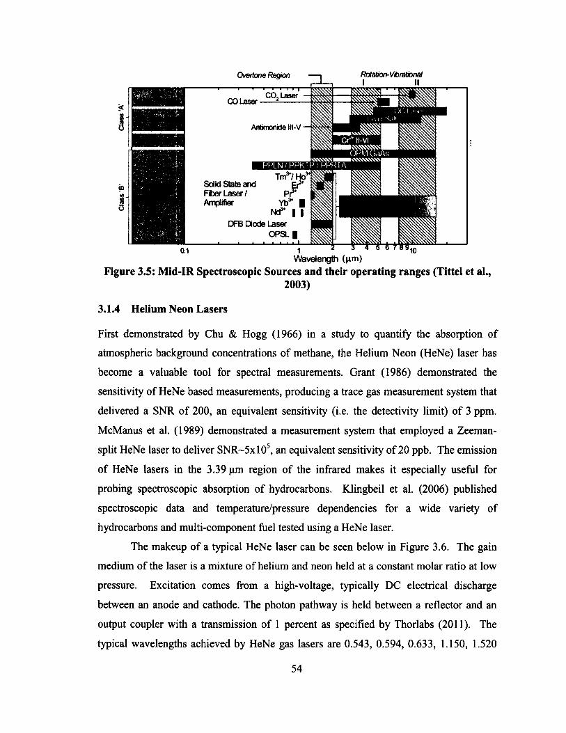
Overtone Region Rotation- Vbrational I II

I f I f I I i | CO. LaserCO Laser

Anhmonde lll-v

QPM GaAs PPLN/PPKIP/PPRIA

Tm /Solid State and Fiber Laser / PiAmplifier Yb* ■

Nd* | |DFB Diode Laser

O PSL |» ‘ » « . . . t

1Wavelength (pm)

Figure 3.5: Mid-IR Spectroscopic Sources and their operating ranges (Tittel et al.,2003)

3.1.4 Helium Neon Lasers

First demonstrated by Chu & Hogg (1966) in a study to quantify the absorption of

atmospheric background concentrations o f methane, the Helium Neon (HeNe) laser has

become a valuable tool for spectral measurements. Grant (1986) demonstrated the

sensitivity o f HeNe based measurements, producing a trace gas measurement system that

delivered a SNR of 200, an equivalent sensitivity (i.e. the detectivity limit) of 3 ppm.

McManus et al. (1989) demonstrated a measurement system that employed a Zeeman-

split HeNe laser to deliver SNR~5xl05, an equivalent sensitivity of 20 ppb. The emission

o f HeNe lasers in the 3.39 pm region o f the infrared makes it especially useful for

probing spectroscopic absorption of hydrocarbons. Klingbeil et al. (2006) published

spectroscopic data and temperature/pressure dependencies for a wide variety of

hydrocarbons and multi-component fuel tested using a HeNe laser.

The makeup of a typical HeNe laser can be seen below in Figure 3.6. The gain

medium of the laser is a mixture o f helium and neon held at a constant molar ratio at low

pressure. Excitation comes from a high-voltage, typically DC electrical discharge

between an anode and cathode. The photon pathway is held between a reflector and an

output coupler with a transmission of 1 percent as specified by Thorlabs (2011). The

typical wavelengths achieved by HeNe gas lasers are 0.543, 0.594, 0.633, 1.150, 1.520

54

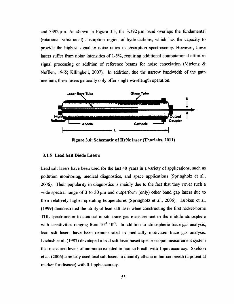
and 3392 pm. As shown in Figure 3.5, the 3.392 pm band overlaps the fundamental

(rotational-vibrational) absorption region of hydrocarbons, which has the capacity to

provide the highest signal to noise ratios in absorption spectroscopy. However, these

lasers suffer from noise intensities o f 1-5%, requiring additional computational effort in

signal processing or addition o f reference beams for noise cancelation (Mielenz &

Nefflen, 1965; Kllingbeil, 2007). In addition, due the narrow bandwidth o f the gain

medium, these lasers generally only offer single wavelength operation.

3.1.5 Lead Salt Diode Lasers

Lead salt lasers have been used for the last 40 years in a variety o f applications, such as

pollution monitoring, medical diagnostics, and space applications (Springholz et al.,

2006). Their popularity in diagnostics is mainly due to the fact that they cover such a

wide spectral range o f 3 to 30 pm and outperform (only) other band gap lasers due to

their relatively higher operating temperatures (Springholz et al., 2006). Lubken et al.

(1999) demonstrated the utility o f lead salt laser when constructing the first rocket-borne

TDL spectrometer to conduct in-situ trace gas measurement in the middle atmosphere

with sensitivities ranging from lO^-lO’5. In addition to atmospheric trace gas analysis,

lead salt lasers have been demonstrated in medically motivated trace gas analysis.

Lachish et al. (1987) developed a lead salt laser-based spectroscopic measurement system

that measured levels o f ammonia exhaled in human breath with lppm accuracy. Skeldon

et al. (2006) similarly used lead salt lasers to quantify ethane in human breath (a potential

marker for disease) with 0 . 1 ppb accuracy.

rOutputCoupler

HighUReflector

Anode

Laser Bore Tube Glass TubeO

/O utputCoupler

L

Figure 3.6: Schematic of HeNe laser (Thorlabs, 2011)

55

The lead salt laser is comprised of a single crystal o f semiconductor material that

is shaped into an optical cavity (Tittel et al., 2003). These materials are generally PbTe,

PbSe and PbS and various alloys of these compounds. To achieve lasing action, a

forward bias current is applied to the p-n junction o f the semiconductor, which populates

the nearly empty conduction band, which in turn stimulates emission across the band gap

(between the conduction and nearly full valence band). Tunability can be achieved by

varying the device temperature or the injection current. The wide tunability and narrow

line width are some o f the major advantages o f the lead salt laser (Springholz et al.,

2006). While many modifications have been made over the years to improve the beam

spatial quality (such as the addition of PbEuSeTe or PbSnTe layers), the main

disadvantage o f the lead salt laser lies in the required operating temperatures o f below

200K in continuous wave mode, limiting the applicability o f this laser in the field (Tittel

et al., 2003).

3.1.6 Quantum Cascade Lasers

While Quantum Cascade Laser (QCL) technology is only a decade old, it has been noted

as a revolutionary mid-IR source o f unprecedented sophistication. Recent notable

applications include the HIAPER Pole-to-Pole Observations (HIPPO) experiment, where

trace gases (more specifically CO2 , CH4 , CO, N 2 O) in the atmosphere were measured

pole to pole over the Pacific/ North America at sub ppb accuracy. This study indicated

several keys areas o f pollution, and provided data that demonstrated global atmospheric

transport modes and their driving mechanisms (Wofsy, 2011). QCL technology has also

been utilized in the medical field to improve the trace gas analysis o f human breath, as

demonstrated by Shorter et al. (2010), where a fully automated QCL spectrometer was

employed to deliver sub-ppb accuracy o f trace gases exhaled through human breath.

While semiconductor lasers employ the band gap between the conduction and

valence bands, QCL’s employ the subbands that exist within the conduction band

quantum wells (Cockbum, 2006). The nature o f this configuration limits radiative losses

and allows for significant optical gains, providing key advantages over conventional Mid-

IR diode lasers (Cockbum, 2006). Tunability o f a QCL is achieved by varying its

56

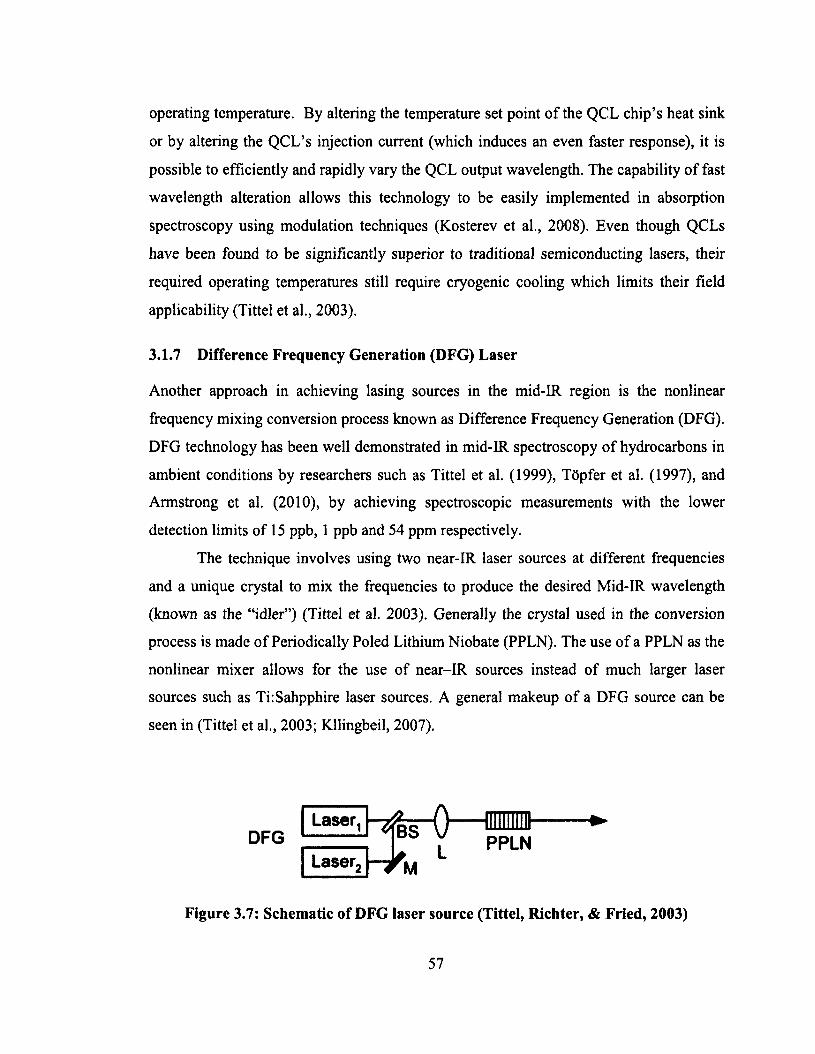
operating temperature. By altering the temperature set point o f the QCL chip’s heat sink

or by altering the QCL’s injection current (which induces an even faster response), it is

possible to efficiently and rapidly vary the QCL output wavelength. The capability o f fast

wavelength alteration allows this technology to be easily implemented in absorption

spectroscopy using modulation techniques (Kosterev et al., 2008). Even though QCLs

have been found to be significantly superior to traditional semiconducting lasers, their

required operating temperatures still require cryogenic cooling which limits their field

applicability (Tittel et al., 2003).

3.1.7 Difference Frequency Generation (DFG) Laser

Another approach in achieving lasing sources in the mid-IR region is the nonlinear

frequency mixing conversion process known as Difference Frequency Generation (DFG).

DFG technology has been well demonstrated in mid-IR spectroscopy of hydrocarbons in

ambient conditions by researchers such as Tittel et al. (1999), Topfer et al. (1997), and

Armstrong et al. (2010), by achieving spectroscopic measurements with the lower

detection limits of 15 ppb, 1 ppb and 54 ppm respectively.

The technique involves using two near-IR laser sources at different frequencies

and a unique crystal to mix the frequencies to produce the desired Mid-IR wavelength

(known as the “idler”) (Tittel et al. 2003). Generally the crystal used in the conversion

process is made of Periodically Poled Lithium Niobate (PPLN). The use o f a PPLN as the

nonlinear mixer allows for the use of near-IR sources instead of much larger laser

sources such as Ti:Sahpphire laser sources. A general makeup o f a DFG source can be

seen in (Tittel et al., 2003; Kllingbeil, 2007).

DFGLaser, h f e - O - — —

h>M 1Laser.

Figure 3.7: Schematic of DFG laser source (Tittel, Richter, & Fried, 2003)

57

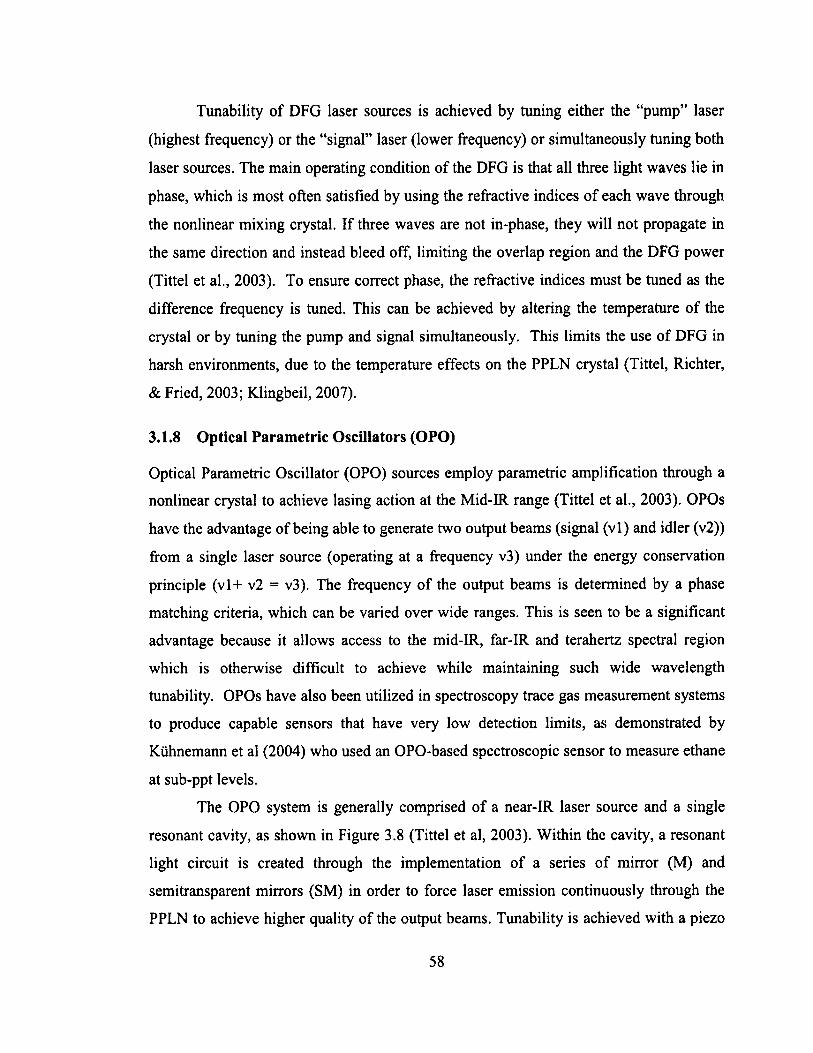
Tunability o f DFG laser sources is achieved by tuning either the “pump” laser

(highest frequency) or the “signal” laser (lower frequency) or simultaneously tuning both

laser sources. The main operating condition of the DFG is that all three light waves lie in

phase, which is most often satisfied by using the refractive indices o f each wave through

the nonlinear mixing crystal. If three waves are not in-phase, they will not propagate in

the same direction and instead bleed off, limiting the overlap region and the DFG power

(Tittel et al., 2003). To ensure correct phase, the refractive indices must be tuned as the

difference frequency is tuned. This can be achieved by altering the temperature of the

crystal or by tuning the pump and signal simultaneously. This limits the use of DFG in

harsh environments, due to the temperature effects on the PPLN crystal (Tittel, Richter,

& Fried, 2003; Klingbeil, 2007).

3.1.8 Optical Parametric Oscillators (OPO)

Optical Parametric Oscillator (OPO) sources employ parametric amplification through a

nonlinear crystal to achieve lasing action at the Mid-IR range (Tittel et al., 2003). OPOs

have the advantage of being able to generate two output beams (signal (v l) and idler (v2 ))

from a single laser source (operating at a frequency v3) under the energy conservation

principle (vl+ v2 = v3). The frequency of the output beams is determined by a phase

matching criteria, which can be varied over wide ranges. This is seen to be a significant

advantage because it allows access to the mid-IR, far-IR and terahertz spectral region

which is otherwise difficult to achieve while maintaining such wide wavelength

tunability. OPOs have also been utilized in spectroscopy trace gas measurement systems

to produce capable sensors that have very low detection limits, as demonstrated by

Kuhnemann et al (2004) who used an OPO-based spectroscopic sensor to measure ethane

at sub-ppt levels.

The OPO system is generally comprised of a near-IR laser source and a single

resonant cavity, as shown in Figure 3.8 (Tittel et al, 2003). Within the cavity, a resonant

light circuit is created through the implementation o f a series o f mirror (M) and

semitransparent mirrors (SM) in order to force laser emission continuously through the

PPLN to achieve higher quality of the output beams. Tunability is achieved with a piezo

58

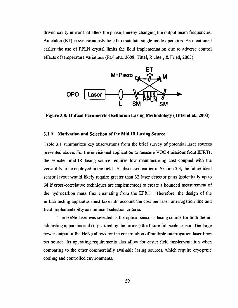
driven cavity mirror that alters the phase, thereby changing the output beam frequencies.

An etalon (ET) is synchronously tuned to maintain single mode operation. As mentioned

earlier the use of PPLN crystal limits the field implementation due to adverse control

effects of temperature variations (Pashotta, 2008; Tittel, Richter, & Fried, 2003).

Figure 3.8: Optical Parametric Oscillation Lasing Methodology (Tittel et al., 2003)

3.1.9 Motivation and Selection of the Mid 1R Lasing Source

Table 3.1 summarizes key observations from the brief survey of potential laser sources

presented above. For the envisioned application to measure VOC emissions from EFRTs,

the selected mid-IR lasing source requires low manufacturing cost coupled with the

versatility to be deployed in the field. As discussed earlier in Section 2.3, the future ideal

sensor layout would likely require greater than 32 laser detector pairs (potentially up to

64 if cross-correlative techniques are implemented) to create a bounded measurement of

the hydrocarbon mass flux emanating from the EFRT. Therefore, the design of the

in-Lab testing apparatus must take into account the cost per laser interrogation line and

field implementabilty as dominant selection criteria.

The HeNe laser was selected as the optical sensor’s lasing source for both the in

lab testing apparatus and (if justified by the former) the future full scale sensor. The large

power output o f the HeNe allows for the construction o f multiple interrogation laser lines

per source. Its operating requirements also allow for easier field implementation when

comparing to the other commercially available lasing sources, which require cryogenic

cooling and controlled environments.

ET

OPO Laser

M+Piezo

59

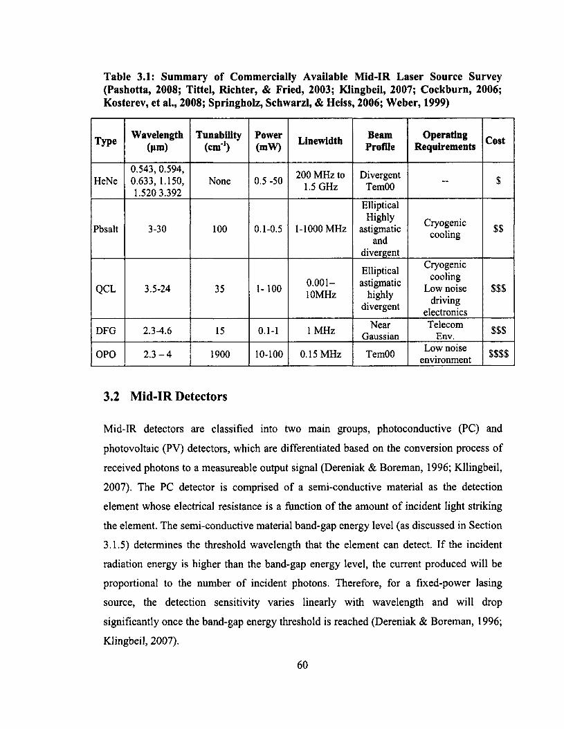
Table 3.1: Summary of Commercially Available Mid-IR Laser Source Survey (Pashotta, 2008; Tittel, Richter, & Fried, 2003; Klingbeil, 2007; Cockburn, 2006; Kosterev, et al., 2008; Springholz, Schwarzl, & Heiss, 2006; Weber, 1999)

Type Wavelength(pm)

Tunability(cm1)

Power(mW) Linewidth Beam

ProfileOperating

Requirements Cost

HeNe0.543, 0.594, 0.633, 1.150, 1.520 3.392

None 0.5 -50 200 MHz to 1.5 GHz

DivergentTemOO -- $

Pbsalt 3-30 100 0.1-0.5 1-1000 MHz

EllipticalHighly

astigmaticand

divergent

Cryogeniccooling $$

QCL 3.5-24 35 1-100 0.001-10MHz

Ellipticalastigmatic

highlydivergent

Cryogenic cooling

Low noise driving

electronics

$$$

DFG 2.3-4.6 15 0.1-1 1 MHz NearGaussian

TelecomEnv. $$$

OPO 2 .3 -4 1900 10-100 0.15 MHz TemOO Low noise environment $$$$

3.2 Mid-IR Detectors

Mid-IR detectors are classified into two main groups, photoconductive (PC) and

photovoltaic (PV) detectors, which are differentiated based on the conversion process of

received photons to a measureable output signal (Dereniak & Boreman, 1996; Kllingbeil,

2007). The PC detector is comprised of a semi-conductive material as the detection

element whose electrical resistance is a function o f the amount o f incident light striking

the element. The semi-conductive material band-gap energy level (as discussed in Section

3.1.5) determines the threshold wavelength that the element can detect. If the incident

radiation energy is higher than the band-gap energy level, the current produced will be

proportional to the number o f incident photons. Therefore, for a fixed-power lasing

source, the detection sensitivity varies linearly with wavelength and will drop

significantly once the band-gap energy threshold is reached (Dereniak & Boreman, 1996;

Klingbeil, 2007).

60

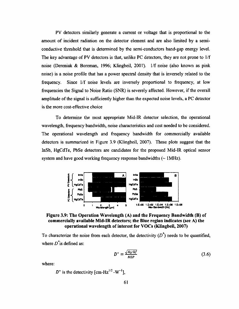
PV detectors similarly generate a current or voltage that is proportional to the

amount o f incident radiation on the detector element and are also limited by a semi-

conductive threshold that is determined by the semi-conductors band-gap energy level.

The key advantage o f PV detectors is that, unlike PC detectors, they are not prone to 1/f

noise (Dereniak & Boreman, 1996; Klingbeil, 2007). 1/f noise (also known as pink

noise) is a noise profile that has a power spectral density that is inversely related to the

frequency. Since 1/f noise levels are inversely proportional to frequency, at low

frequencies the Signal to Noise Ratio (SNR) is severely affected. However, if the overall

amplitude of the signal is sufficiently higher than the expected noise levels, a PC detector

is the more cost-effective choice

To determine the most appropriate Mid-IR detector selection, the operational

wavelength, frequency bandwidth, noise characteristics and cost needed to be considered.

The operational wavelength and frequency bandwidth for commercially available

detectors is summarized in Figure 3.9 (Klingbeil, 2007). These plots suggest that the

InSb, HgCdTe, PbSe detectors are candidates for the proposed Mid-IR optical sensor

system and have good working frequency response bandwidths (~ 1MHz).

HgCdTaHgCdTe

HgCdTeHgCdTe

1 2 3 4W aw langth [pm]

1.E+00 1 .E .02 1.E+04 1.E+06 1.E+M M in Bandwidth [Hz]

Figure 3.9: The Operation Wavelength (A) and the Frequency Bandwidth (B) of commercially available Mid-IR detectors; the Blue region indicates (see A) the

operational wavelength of interest for VOCs (Klingbeil, 2007)

To characterize the noise from each detector, the detectivity (Z)*) needs to be quantified,

where D*is defined as:

D* =NEP

(3.6)

where:

D* is the detectivity [cm-Hz l / 2 -W_1],

61

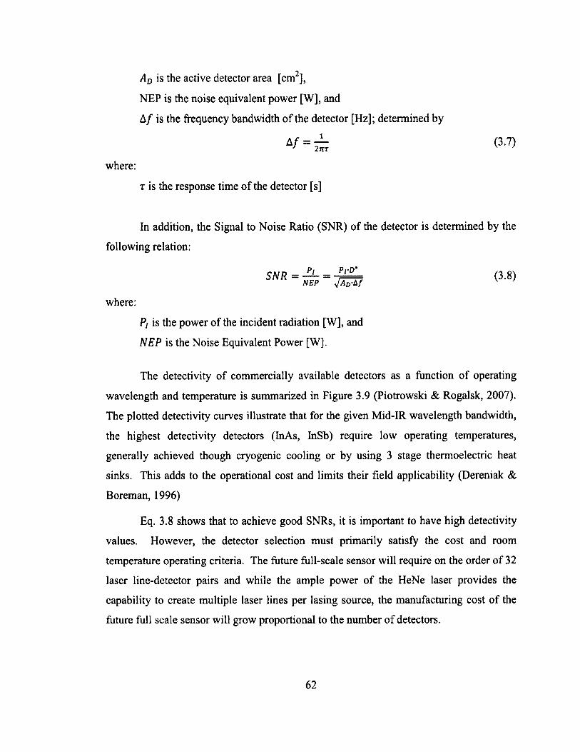
Ad is the active detector area [cm2],

NEP is the noise equivalent power [W], and

A / is the frequency bandwidth o f the detector [Hz]; determined by

Af = T~’ 2m(3.7)

where:

t is the response time o f the detector [s]

In addition, the Signal to Noise Ratio (SNR) of the detector is determined by the

following relation:

Pi is the power o f the incident radiation [W], and

NEP is the Noise Equivalent Power [W],

The detectivity of commercially available detectors as a function of operating

wavelength and temperature is summarized in Figure 3.9 (Piotrowski & Rogalsk, 2007).

The plotted detectivity curves illustrate that for the given Mid-IR wavelength bandwidth,

the highest detectivity detectors (InAs, InSb) require low operating temperatures,

generally achieved though cryogenic cooling or by using 3 stage thermoelectric heat

sinks. This adds to the operational cost and limits their field applicability (Dereniak &

Boreman, 1996)

Eq. 3.8 shows that to achieve good SNRs, it is important to have high detectivity

values. However, the detector selection must primarily satisfy the cost and room

temperature operating criteria. The future full-scale sensor will require on the order of 32

laser line-detector pairs and while the ample power of the HeNe laser provides the

capability to create multiple laser lines per lasing source, the manufacturing cost of the

future full scale sensor will grow proportional to the number o f detectors.

SNR = -fr-Pj PyD' (3.8)

NEP y/AD-bf

where:

62

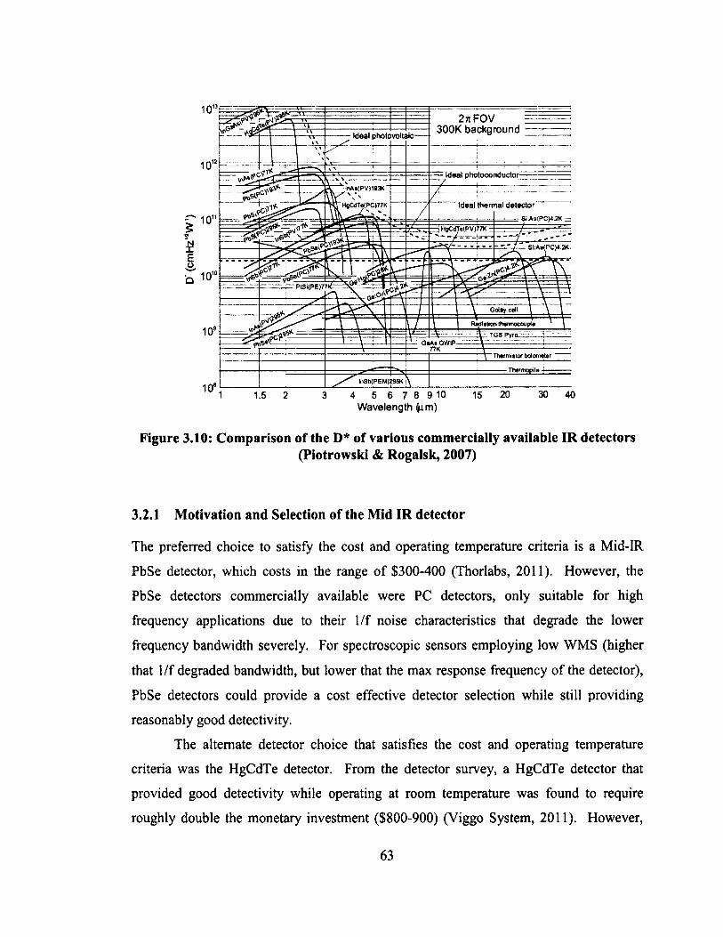
2 j iF0V 300K background

7 ideal photovoltaic

Ideal p h o toconduc to r

Ideal therm al d e te c to r '

Golay call

TGS Pyra:

Thermistor bolometer

Wavelength m)

Figure 3.10: Comparison of the D* of various commercially available IR detectors(Piotrowski & Rogalsk, 2007)

3.2.1 Motivation and Selection of the Mid IR detector

The preferred choice to satisfy the cost and operating temperature criteria is a Mid-IR

PbSe detector, which costs in the range of $300-400 (Thorlabs, 2011). However, the

PbSe detectors commercially available were PC detectors, only suitable for high

frequency applications due to their 1 /f noise characteristics that degrade the lower

frequency bandwidth severely. For spectroscopic sensors employing low WMS (higher

that 1 /f degraded bandwidth, but lower that the max response frequency of the detector),

PbSe detectors could provide a cost effective detector selection while still providing

reasonably good detectivity.

The alternate detector choice that satisfies the cost and operating temperature

criteria was the HgCdTe detector. From the detector survey, a HgCdTe detector that

provided good detectivity while operating at room temperature was found to require

roughly double the monetary investment ($800-900) (Viggo System, 2011). However,

63

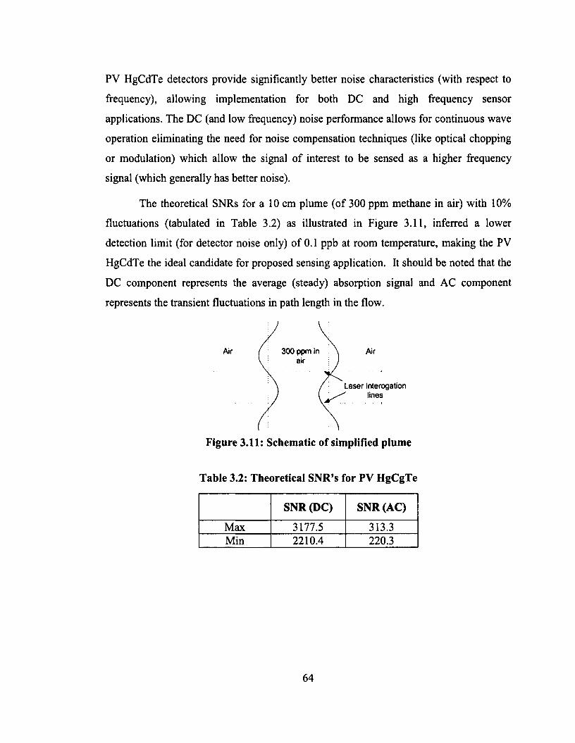
PV HgCdTe detectors provide significantly better noise characteristics (with respect to

frequency), allowing implementation for both DC and high frequency sensor

applications. The DC (and low frequency) noise performance allows for continuous wave

operation eliminating the need for noise compensation techniques (like optical chopping

or modulation) which allow the signal of interest to be sensed as a higher frequency

signal (which generally has better noise).

The theoretical SNRs for a 10 cm plume (of 300 ppm methane in air) with 10%

fluctuations (tabulated in Table 3.2) as illustrated in Figure 3.11, inferred a lower

detection limit (for detector noise only) of 0.1 ppb at room temperature, making the PV

HgCdTe the ideal candidate for proposed sensing application. It should be noted that the

DC component represents the average (steady) absorption signal and AC component

represents the transient fluctuations in path length in the flow.

300 ppm in air

Air

Laser Interrogation lines

Figure 3.11: Schematic of simplified plume

Table 3.2: Theoretical SNR’s for PV HgCgTe

SNR (DC) SNR (AC)

Max 3177.5 313.3Min 2210.4 220.3

64

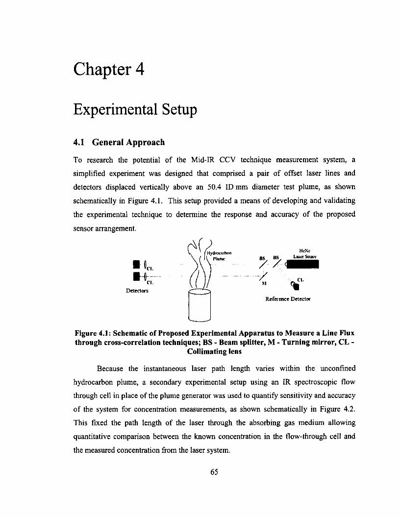
Chapter 4

Experimental Setup

4.1 General Approach

To research the potential of the Mid-IR CCV technique measurement system, a

simplified experiment was designed that comprised a pair o f offset laser lines and

detectors displaced vertically above an 50.4 ID mm diameter test plume, as shown

schematically in Figure 4.1. This setup provided a means o f developing and validating

the experimental technique to determine the response and accuracy of the proposed

sensor arrangement.

Figure 4.1: Schematic of Proposed Experimental Apparatus to Measure a Line Flux through cross-correlation techniques; BS - Beam splitter, M - Turning mirror, CL -

Because the instantaneous laser path length varies within the unconfined

hydrocarbon plume, a secondary experimental setup using an IR spectroscopic flow

through cell in place of the plume generator was used to quantify sensitivity and accuracy

of the system for concentration measurements, as shown schematically in Figure 4.2.

This fixed the path length o f the laser through the absorbing gas medium allowing

quantitative comparison between the known concentration in the flow-through cell and

the measured concentration from the laser system.

Hydrocarbon I Plume

Reference Detector

Collimating lens

65

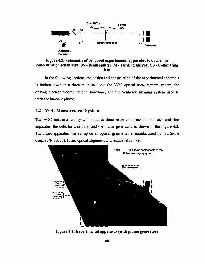
M IR flow through ctll CLDetectors

ReferenceDetector

Figure 4.2: Schematic of proposed experimental apparatus to determine concentration sensitivity; BS - Beam splitter, M - Turning mirror, CS - Collimating

lens

In the following sections, the design and construction o f the experimental apparatus

is broken down into three main sections: the VOC optical measurement system, the

driving electronic/computational hardware, and the Schlieren imaging system used to

track the buoyant plume.

4.2 VOC Measurement System

The VOC measurement system includes three main components: the laser emission

apparatus, the detector assembly, and the plume generator, as shown in the Figure 4.3.

The entire apparatus was set up on an optical granite table manufactured by Tru Stone

Corp. (S/N 30737), to aid optical alignment and reduce vibrations.

- — indicates components of the Schieren imaging system

(Detector Assembly ]

( Plume H I Generator (~

i Lasing I I Assembly j

Figure 4.3: Experimental apparatus (with plume generator)

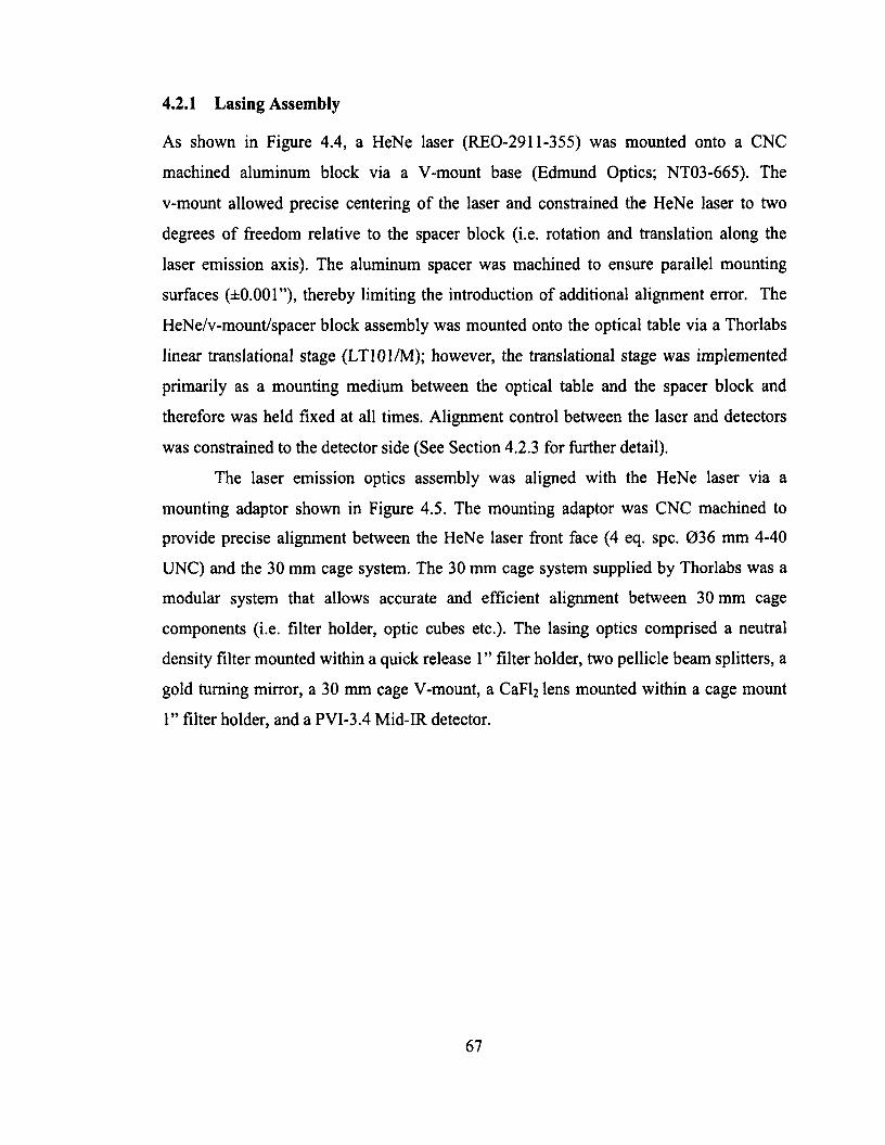
4.2.1 Lasing Assembly

As shown in Figure 4.4, a HeNe laser (REO-2911-355) was mounted onto a CNC

machined aluminum block via a V-mount base (Edmund Optics; NT03-665). The

v-mount allowed precise centering o f the laser and constrained the HeNe laser to two

degrees of freedom relative to the spacer block (i.e. rotation and translation along the

laser emission axis). The aluminum spacer was machined to ensure parallel mounting

surfaces (±0.001”), thereby limiting the introduction of additional alignment error. The

HeNe/v-mount/spacer block assembly was mounted onto the optical table via a Thorlabs

linear translational stage (LT101/M); however, the translational stage was implemented

primarily as a mounting medium between the optical table and the spacer block and

therefore was held fixed at all times. Alignment control between the laser and detectors

was constrained to the detector side (See Section 4.2.3 for further detail).

The laser emission optics assembly was aligned with the HeNe laser via a

mounting adaptor shown in Figure 4.5. The mounting adaptor was CNC machined to

provide precise alignment between the HeNe laser front face (4 eq. spc. 036 mm 4-40

UNC) and the 30 mm cage system. The 30 mm cage system supplied by Thorlabs was a

modular system that allows accurate and efficient alignment between 30 mm cage

components (i.e. filter holder, optic cubes etc.). The lasing optics comprised a neutral

density filter mounted within a quick release 1 ” filter holder, two pellicle beam splitters, a

gold turning mirror, a 30 mm cage V-mount, a CaFl2 lens mounted within a cage mount

1” filter holder, and a PVI-3.4 Mid-IR detector.

67

V mount

Thermistor

Alignment adapter

HeNE laser

Neutral DensityFilter

Beam Splitters

PVI-3.4 Dectector

Machined aluminum spacer

Thorlabs 30mm cage system

90’ T u rn in g M irro r

Figure 4.4: Lasing assembly of the VOC measurement sensor

Figure 4.5: HeNe Laser - 30 mm cage alignment adapter

The 0.3 Optical Density (OD) neutral density filter (Edmund optics; NT64-353) is

mounted onto the 30mm cage system (Thorlabs) between the He-Ne laser and the first

pellicle beam splitter via a quick release 1” optic holder (Thorlabs; QRC1A). The filter

68

has a flat transmission (-46%) curve across the experimental spectral bandwidth, as

shown in Figure 4.6. This ensures that all three detectors (Vigo System; PVI-3.4) operate

below their saturation limits (of lmW/mm2) even at the HeNe’s max operating power of

5mW.

Pellicle beam splitters were used to split the incoming laser intensity among the

reference detector and the two detection lines. They are documented by Thorlabs (2010)

and mentioned by Lyle (2005) to be the best choice when dispersion must be kept to a

minimum. They virtually eliminate multiple reflections that are commonly seen with the

use of thicker glass beam splitters known as ghosting. This phenomenon develops due to

the secondary reflection within the optic and causes increased optical power losses and a

secondary beam that is displaced from the original beam by the thickness of the optic.

However, they are immensely fragile and can be easily destroyed or damaged through

any surface contact. Through the use of Thorlabs beam splitter 30 mm cage cubes, the

pellicle beam splitter can be protected and implemented into the in-lab sensor design

without risk of damage. The pellicle beam splitters are also a viable choice for the future

field sensor so long as additional precautions are taken to ensure safety from the

atmospheric particulates.

The first pellicle beam splitter (Thorlabs; CM1-BP145B4) directs a portion o f the

laser intensity onto the reference detector. As noted earlier, the Mid-IR detector, v-block

mounting platform, CaFl2 lens and pellicle beam splitter cube were held rigidly together

using the 30 mm cage system, ensuring proper alignment the optical components along

the laser propagation axis. To ensure proper focusing of the laser light onto the detector’s

active area, an /= 40m m CaFl2 Plano-convex lens (Thorlabs; LA5370-E) with a

specialized Anti-Reflective (AR) coating was utilized. The AR coating acts as a weak

band pass filter across the (3-5 pm) Mid-IR region. The detector V-mount platform

(Thorlabs; ARV1) was used to align and centre the detector with the focal point o f the

CaFl2 lens within the 30 mm cage, preventing power losses through misalignment. The

spectral response curves for the AR coated CaFl2 lens and the PVI-3.4 (HgCdTe) detector

can be seen in Figure 4.7.

69

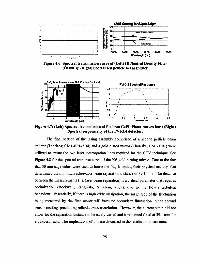
100

I? *0

4&8S Coating lor 3.0|int-5.0|im

oo40

20

tran« fittanca

• Reflet lance

5000 5400 3800 4200 4600 5000Wsvolongth (nm)

Figure 4.6: Spectral transmission curve of (Left) IR Neutral Density Filter (OD=0.3); (Right) Specialized pellicle beam splitter

CaF, Total T ranarnhtlonJA R Coaling: 3 - 5 f n )PVI-3.4 Spoctral Response

2.5

2

1.5

5 -0.5

02.5 3.52 3 4 4.5

W avalangth (|*n)

Figure 4.7: (Left) Spectral transmission of f=40mm CaFh Plano-convex lens; (Right) Spectral responsivity of the PVI-3.4 detector.

The final section o f the lasing assembly comprised o f a second pellicle beam

splitter (Thorlabs; CM1-BP145B4) and a gold plated mirror (Thorlabs; CM1-M01) were

utilized to create the two laser interrogation lines required for the CCV technique. See

Figure 4.8 for the spectral response curve o f the 90° gold turning mirror. Due to the fact

that 30 mm cage cubes were used to house the fragile optics, their physical makeup also

determined the minimum achievable beam separation distance o f 39.1 mm. The distance

between the measurements (i.e. laser beam separation) is a critical parameter that requires

optimization (Rockwell, Rangwala, & Klein, 2009), due to the flow’s turbulent

behaviour. Essentially, if there is high eddy dissipation, the magnitude o f the fluctuation

being measured by the first sensor will have no secondary fluctuation in the second

sensor reading, precluding reliable cross-correlation. However, the current setup did not

allow for the separation distance to be easily varied and it remained fixed at 39.1 mm for

all experiments. The implications o f this are discussed in the results and discussion.

70

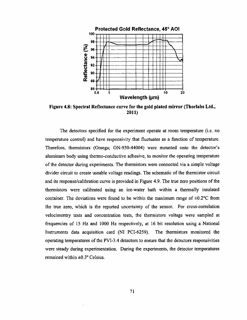
Protected Gold Reflectance, 45° AOI100

ooc2o0)

10 200.6 1Wavelength (pm)

Figure 4.8: Spectral Reflectance curve for the gold plated mirror (Thorlabs Ltd.,2011)

The detectors specified for the experiment operate at room temperature (i.e. no

temperature control) and have responsivity that fluctuates as a function of temperature.

Therefore, thermistors (Omega; ON-930-44004) were mounted onto the detector’s

aluminum body using thermo-conductive adhesive, to monitor the operating temperature

of the detector during experiments. The thermistors were connected via a simple voltage

divider circuit to create useable voltage readings. The schematic o f the thermistor circuit

and its response/calibration curve is provided in Figure 4.9. The true zero positions o f the

thermistors were calibrated using an ice-water bath within a thermally insulated

container. The deviations were found to be within the maximum range o f ±0.2°C from

the true zero, which is the reported uncertainty of the sensor. For cross-correlation

velocimentry tests and concentration tests, the thermistors voltage were sampled at

frequencies o f 15 Hz and 1000 Hz respectively, at 16 bit resolution using a National

Instruments data acquisition card (NI PCI-6259). The thermistors monitored the

operating temperatures o f the PVI-3.4 detectors to ensure that the detectors responsivities

were steady during experimentation. During the experiments, the detector temperatures

remained within ±0.3° Celsius.

71

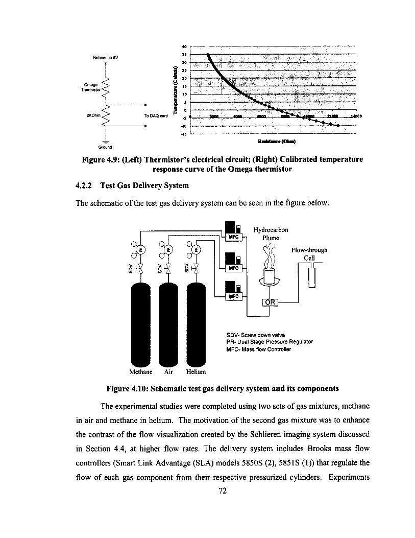
Reference 5V

OmegaThermistor ■*

2KOhm« To DAQ card

40

30

B«>a 10

.10

-15

R aW N ce(O fcH )Ground

Figure 4.9: (Left) Thermistor’s electrical circuit; (Right) Calibrated temperature response curve of the Omega thermistor

4.2.2 Test Gas Delivery System

The schematic o f the test gas delivery system can be seen in the figure below.

> ,

8 1 5</3

■■H MFC h

- f c

HydrocarbonPlume

Flow-through Cell ~1T~

OFT

SDV- Screw down valvePR- Dual Stage Pressure RegulatorMFC- Mass flow Controller

Methane Air Helium

Figure 4.10: Schematic test gas delivery system and its components

The experimental studies were completed using two sets of gas mixtures, methane

in air and methane in helium. The motivation of the second gas mixture was to enhance

the contrast o f the flow visualization created by the Schlieren imaging system discussed

in Section 4.4, at higher flow rates. The delivery system includes Brooks mass flow

controllers (Smart Link Advantage (SLA) models 5850S (2), 5851S (1)) that regulate the

flow of each gas component from their respective pressurized cylinders. Experiments

72

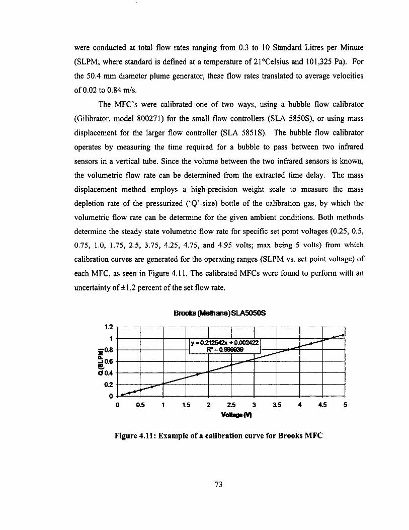
were conducted at total flow rates ranging from 0.3 to 10 Standard Litres per Minute

(SLPM; where standard is defined at a temperature of 21 “Celsius and 101,325 Pa). For

the 50.4 mm diameter plume generator, these flow rates translated to average velocities

of 0.02 to 0.84 m/s.

The MFC’s were calibrated one o f two ways, using a bubble flow calibrator

(Gilibrator, model 800271) for the small flow controllers (SLA 5850S), or using mass

displacement for the larger flow controller (SLA 585IS). The bubble flow calibrator

operates by measuring the time required for a bubble to pass between two infrared

sensors in a vertical tube. Since the volume between the two infrared sensors is known,

the volumetric flow rate can be determined from the extracted time delay. The mass

displacement method employs a high-precision weight scale to measure the mass

depletion rate o f the pressurized (‘Q ’-size) bottle of the calibration gas, by which the

volumetric flow rate can be determine for the given ambient conditions. Both methods

determine the steady state volumetric flow rate for specific set point voltages (0.25, 0.5,

0.75, 1.0, 1.75, 2.5, 3.75, 4.25, 4.75, and 4.95 volts; max being 5 volts) from which

calibration curves are generated for the operating ranges (SLPM vs. set point voltage) of

each MFC, as seen in Figure 4.11. The calibrated MFCs were found to perform with an

uncertainty of ±1.2 percent o f the set flow rate.

Brooks (Mettiane)SLA5050S

1.2

y = 0212542X + 0.002422 R*=0.909939

0 0 .4

02

as 4 45 50 0.5 1 1.5 2 3Voltage (V)

Figure 4.11: Example of a calibration curve for Brooks MFC

73

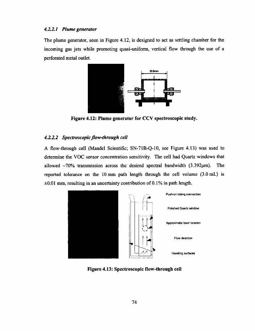
4.2.2.1 Plume generator

The plume generator, seen in Figure 4.12, is designed to act as settling chamber for the

incoming gas jets while promoting quasi-uniform, vertical flow through the use of a

perforated metal outlet.

50.amm |

- U - JI Ii i f e s i

Figure 4.12: Plume generator for CCV spectroscopic study.

4.2.2.2 Spectroscopic flow-through cell

A flow-through cell (Mandel Scientific; SN-71B-Q-10, see Figure 4.13) was used to

determine the VOC sensor concentration sensitivity. The cell had Quartz windows that

allowed -70% transmission across the desired spectral bandwidth (3.392pm). The

reported tolerance on the 10 mm path length through the cell volume (3.0 mL) is

±0.01 mm, resulting in an uncertainty contribution o f 0.1% in path length.

Push-on tubing connectors

Polished Quartz window

Approximate laser location

Flow direction

VHandling surfaces

Figure 4.13: Spectroscopic flow-through cell

74

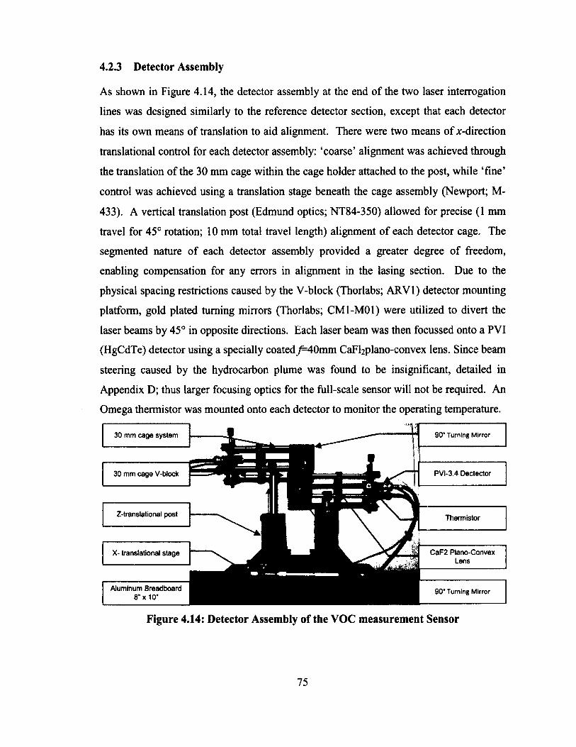
4.2.3 Detector Assembly

As shown in Figure 4.14, the detector assembly at the end o f the two laser interrogation

lines was designed similarly to the reference detector section, except that each detector

has its own means of translation to aid alignment. There were two means o f x-direction

translational control for each detector assembly: ‘coarse’ alignment was achieved through

the translation of the 30 mm cage within the cage holder attached to the post, while ‘fine’

control was achieved using a translation stage beneath the cage assembly (Newport; M-

433). A vertical translation post (Edmund optics; NT84-350) allowed for precise (1 mm

travel for 45° rotation; 10 mm total travel length) alignment o f each detector cage. The

segmented nature o f each detector assembly provided a greater degree o f freedom,

enabling compensation for any errors in alignment in the lasing section. Due to the

physical spacing restrictions caused by the V-block (Thorlabs; ARV1) detector mounting

platform, gold plated turning mirrors (Thorlabs; CM1-M01) were utilized to divert the

laser beams by 45° in opposite directions. Each laser beam was then focussed onto a PVI

(HgCdTe) detector using a specially coated/=40mm CaF^plano-convex lens. Since beam

steering caused by the hydrocarbon plume was found to be insignificant, detailed in

Appendix D; thus larger focusing optics for the full-scale sensor will not be required. An

Omega thermistor was mounted onto each detector to monitor the operating temperature.

9 0 ‘ T urn ing M irro r30 mm cage system

PVI-3.4 Dectector

Z-translational post Thermistor

CaF2 Plano-Convex Lens

X- translational stage

Aluminum Breadboard 8" x 10”

9 0 ' T urn ing M irro r

Figure 4.14: Detector Assembly of the VOC measurement Sensor

75

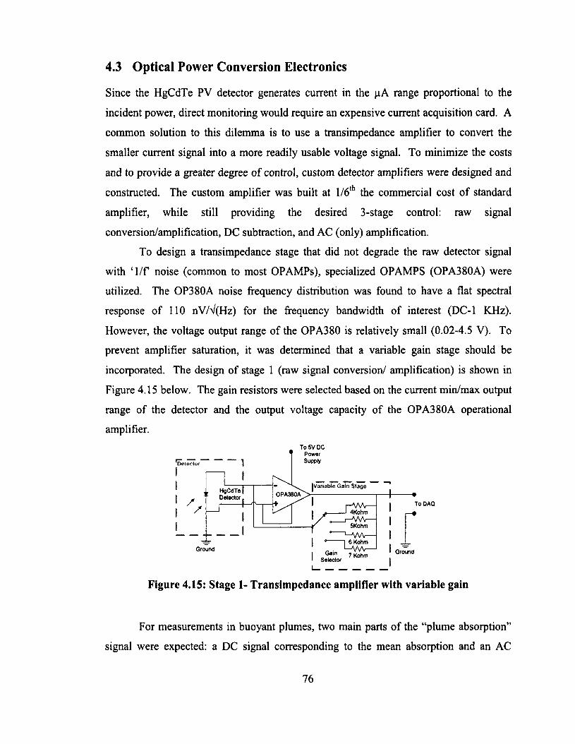
4.3 Optical Power Conversion Electronics

Since the HgCdTe PV detector generates current in the pA range proportional to the

incident power, direct monitoring would require an expensive current acquisition card. A

common solution to this dilemma is to use a transimpedance amplifier to convert the

smaller current signal into a more readily usable voltage signal. To minimize the costs

and to provide a greater degree o f control, custom detector amplifiers were designed and

constructed. The custom amplifier was built at l/6 th the commercial cost o f standard

amplifier, while still providing the desired 3-stage control: raw signal

conversion/amplification, DC subtraction, and AC (only) amplification.

To design a transimpedance stage that did not degrade the raw detector signal

with ‘1 /f noise (common to most OPAMPs), specialized OP AMPS (OPA380A) were

utilized. The OP380A noise frequency distribution was found to have a flat spectral

response o f 110 nV/V(Hz) for the frequency bandwidth o f interest (DC-1 KHz).

However, the voltage output range o f the OPA380 is relatively small (0.02-4.5 V). To

prevent amplifier saturation, it was determined that a variable gain stage should be

incorporated. The design o f stage 1 (raw signal conversion/ amplification) is shown in

Figure 4.15 below. The gain resistors were selected based on the current min/max output

range of the detector and the output voltage capacity o f the OPA380A operational

amplifier.

PowerSupplyD etector

|V a riab le G ain S tag eH gCdTe| Detector. OPA380A

To DAQrVA— J 4Kohm

5Kohm

0--------- 1 6 Kohm'—vw—

o 0ain 7 Kohm Selector

Ground Ground

Figure 4.15: Stage 1- Transimpedance amplifier with variable gain

For measurements in buoyant plumes, two main parts o f the “plume absorption”

signal were expected: a DC signal corresponding to the mean absorption and an AC

76

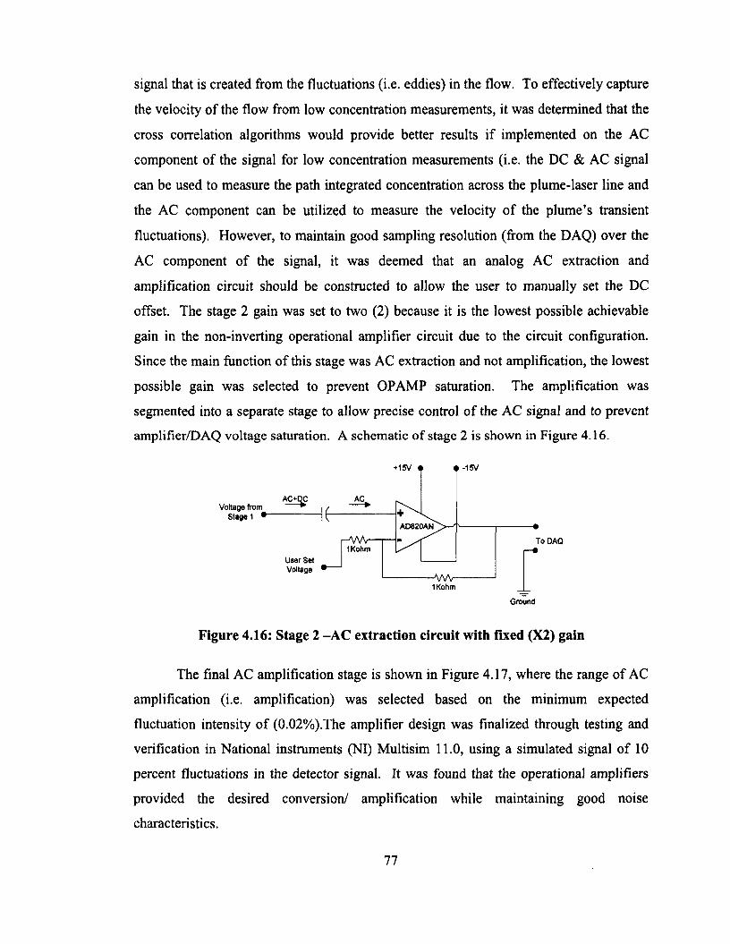
signal that is created from the fluctuations (i.e. eddies) in the flow. To effectively capture

the velocity o f the flow from low concentration measurements, it was determined that the

cross correlation algorithms would provide better results if implemented on the AC

component of the signal for low concentration measurements (i.e. the DC & AC signal

can be used to measure the path integrated concentration across the plume-laser line and

the AC component can be utilized to measure the velocity o f the plume’s transient

fluctuations). However, to maintain good sampling resolution (from the DAQ) over the

AC component o f the signal, it was deemed that an analog AC extraction and

amplification circuit should be constructed to allow the user to manually set the DC

offset. The stage 2 gain was set to two (2) because it is the lowest possible achievable

gain in the non-inverting operational amplifier circuit due to the circuit configuration.

Since the main function of this stage was AC extraction and not amplification, the lowest

possible gain was selected to prevent OP AMP saturation. The amplification was

segmented into a separate stage to allow precise control o f the AC signal and to prevent

amplifier/DAQ voltage saturation. A schematic o f stage 2 is shown in Figure 4.16.

+15V • • -15V

AC+DCVoltage from_ ►

S tag e 1 •

AC.

AD820AN

HWV1Kohm

To DAQ

U ser S et Voltage

•AAAr1Kohm

Ground

Figure 4.16: Stage 2 -AC extraction circuit with fixed (X2) gain

The final AC amplification stage is shown in Figure 4.17, where the range of AC

amplification (i.e. amplification) was selected based on the minimum expected

fluctuation intensity o f (0.02%).The amplifier design was finalized through testing and

verification in National instruments (NI) Multisim 11.0, using a simulated signal o f 10

percent fluctuations in the detector signal. It was found that the operational amplifiers

provided the desired conversion/ amplification while maintaining good noise

characteristics.

77

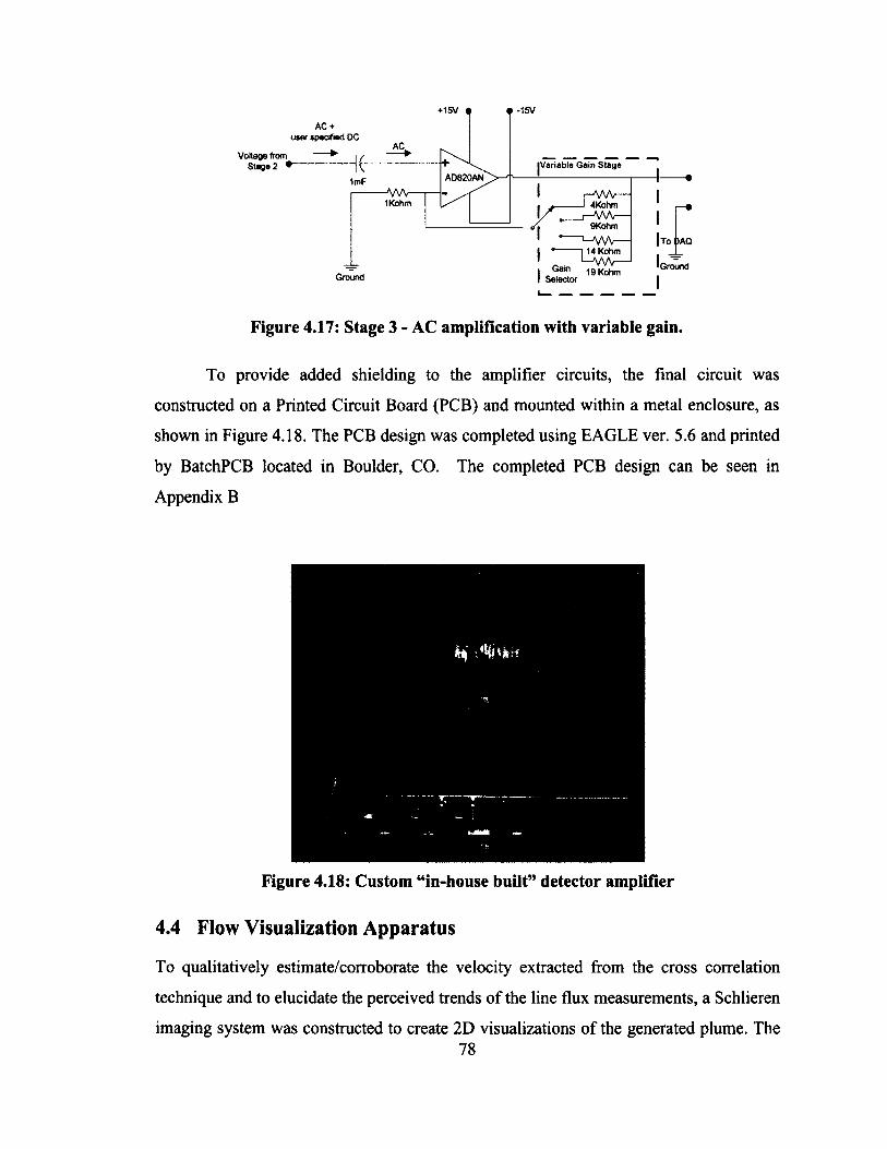
+15V • • -15V

AC + user specified DC

AC.Voltage from

Stage 2 * Variable Gain S tageAD820AN1mF

AAA1Kohm

r~AAAr—- J 4Kohm

SKohm

To >AQ°---------1 14 Kohm. . L-A/W—Gam 19 Kohm

SelectorGround

Ground

Figure 4.17: Stage 3 - AC amplification with variable gain.

To provide added shielding to the amplifier circuits, the final circuit was

constructed on a Printed Circuit Board (PCB) and mounted within a metal enclosure, as

shown in Figure 4.18. The PCB design was completed using EAGLE ver. 5.6 and printed

by BatchPCB located in Boulder, CO. The completed PCB design can be seen in

Appendix B

Figure 4.18: Custom “in-house built” detector amplifier

4.4 Flow Visualization Apparatus

To qualitatively estimate/corroborate the velocity extracted from the cross correlation

technique and to elucidate the perceived trends o f the line flux measurements, a Schlieren

imaging system was constructed to create 2D visualizations o f the generated plume. The78

Schlieren imaging technique utilizes the fundamental linear relationship between the

refractive index and the gas density (e.g. Settles (2001), to produce contrast images that

are proportional to the spatial density gradients. The methodology requires parallel light

rays to pass through the ‘test section’ (of different gas density than air) which in turn

causes some light rays to bend away from their original path. As seen in Figure 4.19, the

light passes through a (non-air) gas pocket which causes it to refract onto a new path ‘B \

Then by focusing the light onto an opaque filter (more commonly known as a knife-edge)

that lies just outside the focal point, an image with a dark spot corresponding to the

‘blocked’ light can be generated. However, a Schlieren object refracts many such rays in

many directions, the downward rays are blocked off and the top rays are not and

propagate to the image plane. The overlay o f the blocked light and the refracted light

yields a gradient o f the refraction that is also proportional to the gradient o f density

(Atcheson, 2007; Settles, 2001). The percent o f light cut-off by the knife yields Schlieren

images with proportional contrast and by that effect allows discerning o f smaller density

gradients. By using a vertical knife edge, a horizontal density gradient image can be

generated because all the light refracted onto new angles on the horizontal plane will be

blocked by the knife edge and vice-versa.

Refractive index field

Image | p lana |

Light n source

Filter

Figure 4.19: A simple lens-based Schlieren setup (Atcheson, 2007)

79

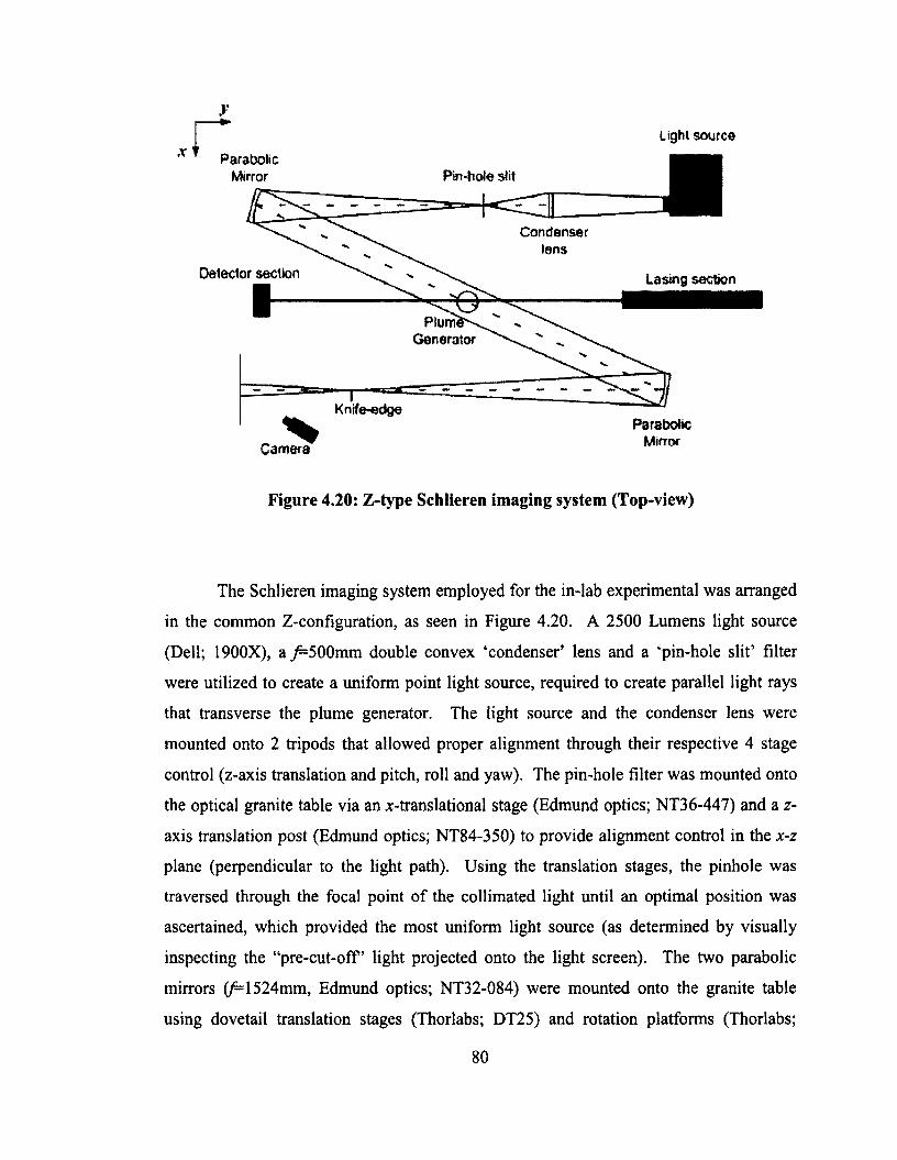
,v t

y

ParabolicMirror

Light source

Pin-hole slit

Detector section Lasing section

PIGenerator

Knife-edge

Camera

ParabolicMirror

Figure 4.20: Z-type Schlieren imaging system (Top-view)

The Schlieren imaging system employed for the in-lab experimental was arranged

in the common Z-configuration, as seen in Figure 4.20. A 2500 Lumens light source

(Dell; 1900X), a /=500mm double convex ‘condenser’ lens and a ‘pin-hole slit’ filter

were utilized to create a uniform point light source, required to create parallel light rays

that transverse the plume generator. The light source and the condenser lens were

mounted onto 2 tripods that allowed proper alignment through their respective 4 stage

control (z-axis translation and pitch, roll and yaw). The pin-hole filter was mounted onto

the optical granite table via an x-translational stage (Edmund optics; NT36-447) and a z-

axis translation post (Edmund optics; NT84-350) to provide alignment control in the x-z

plane (perpendicular to the light path). Using the translation stages, the pinhole was

traversed through the focal point of the collimated light until an optimal position was

ascertained, which provided the most uniform light source (as determined by visually

inspecting the “pre-cut-off’ light projected onto the light screen). The two parabolic

mirrors (J= 1524mm, Edmund optics; NT32-084) were mounted onto the granite table

using dovetail translation stages (Thorlabs; DT25) and rotation platforms (Thorlabs;

80

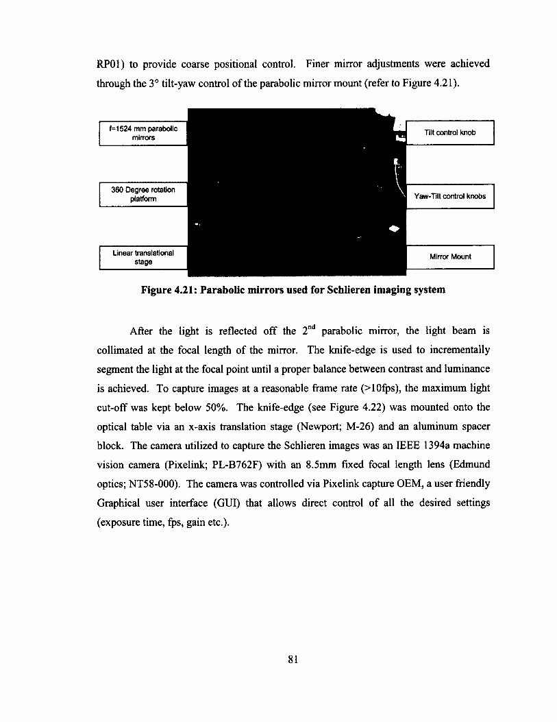
RP01) to provide coarse positional control. Finer mirror adjustments were achieved

through the 3° tilt-yaw control of the parabolic mirror mount (refer to Figure 4.21).

f=1524 mm parabolic mirrors Tilt control knob

360 Degree rotation platform Yaw-Tilt control knobs

Linear translational stage Mirror Mount

Figure 4.21: Parabolic mirrors used for Schlieren imaging system

After the light is reflected off the 2nd parabolic mirror, the light beam is

collimated at the focal length o f the mirror. The knife-edge is used to incrementally

segment the light at the focal point until a proper balance between contrast and luminance

is achieved. To capture images at a reasonable frame rate (>10fps), the maximum light

cut-off was kept below 50%. The knife-edge (see Figure 4.22) was mounted onto the

optical table via an x-axis translation stage (Newport; M-26) and an aluminum spacer

block. The camera utilized to capture the Schlieren images was an IEEE 1394a machine

vision camera (Pixelink; PL-B762F) with an 8.5mm fixed focal length lens (Edmund

optics; NT58-000). The camera was controlled via Pixelink capture OEM, a user friendly

Graphical user interface (GUI) that allows direct control o f all the desired settings

(exposure time, Ips, gain etc.).

81

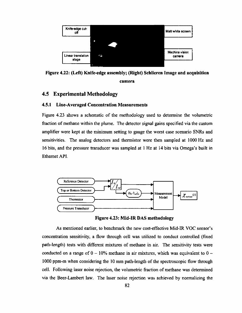
Knife-edge cutoff Matt white screen

Machine vision cameraLinear translation

stage

Figure 4.22: (Left) Knife-edge assembly; (Right) Schlieren Image and acquisition

camera

4.5 Experimental Methodology

4.5.1 Line-Averaged Concentration Measurements

Figure 4.23 shows a schematic o f the methodology used to determine the volumetric

fraction of methane within the plume. The detector signal gains specified via the custom

amplifier were kept at the minimum setting to gauge the worst case scenario SNRs and

sensitivities. The analog detectors and thermistor were then sampled at 1000 Hz and

16 bits, and the pressure transducer was sampled at 1 Hz at 14 bits via Omega’s built in

Ethernet API.

C Reference Detector

( t*

ccor Bottom Detector

Thermistor

Pressure Transducer

>>>>

Measurement Model ■> Z- (t)

Figure 4.23: Mid-IR DAS methodology

As mentioned earlier, to benchmark the new cost-effective Mid-IR VOC sensor’s

concentration sensitivity, a flow through cell was utilized to conduct controlled (fixed

path-length) tests with different mixtures o f methane in air. The sensitivity tests were

conducted on a range o f 0 - 10% methane in air mixtures, which was equivalent to 0 -

1000 ppm-m when considering the 10 mm path-length of the spectroscopic flow through

cell. Following laser noise rejection, the volumetric fraction o f methane was determined

via the Beer-Lambert law. The laser noise rejection was achieved by normalizing the

82

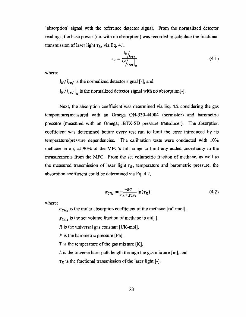
‘absorption’ signal with the reference detector signal. From the normalized detector

readings, the base power (i.e. with no absorption) was recorded to calculate the fractional

transmission of laser light rR, via Eq. 4.1.

In / I ref is the normalized detector signal [-], and

In/Ire f \0 is the normalized detector signal with no absorption[-].

Next, the absorption coefficient was determined via Eq. 4.2 considering the gas

temperature(measured with an Omega ON-930-44004 thermistor) and barometric

pressure (measured with an Omega; iBTX-SD pressure transducer). The absorption

coefficient was determined before every test run to limit the error introduced by its

temperature/pressure dependencies. The calibration tests were conducted with 10%

methane in air, at 90% of the MFC’s full range to limit any added uncertainty in the

measurements from the MFC. From the set volumetric fraction o f methane, as well as

the measured transmission of laser light t r , temperature and barometric pressure, the

absorption coefficient could be determined via Eq. 4.2,

where:aCHi is the molar absorption coefficient o f the methane [m2 /mol],

XcHt is the set volume fraction of methane in air[-],

R is the universal gas constant [J/K-mol],

P is the barometric pressure [Pa],

T is the temperature o f the gas mixture [K],

L is the traverse laser path length through the gas mixture [m], and

xR is the fractional transmission of the laser light [-].

(4.1)

where:

83

4.5.1.1 Uncertainty analysis o f o Cha and X cha

The total uncertainties o f the measured absorption coefficient crCH4 and volumetric

fraction Xch4 were calculated in accordance with the ANSI/ASME Measurement

uncertainty standard [1985]. The standard utilizes the Taylor Series Method (TSM)

method to combine the systematic and precision errors o f each measured variable to

estimate a final total uncertainty. The systematic error (more commonly known as the

bias error) is a measure of an instrument’s inability to measure the true value. Precision

error on the other hand is the random error or scatter of a repeated measurement. It

should be noted that this approach is only directly applicable to measurements with

Gaussian error distributions. The calculation of total uncertainty using the TSM method

of combining component uncertainties can be seen in Eq. 4.3. (Coleman, 2009)

v - ( t ) 2 + ( £ ) 2 “i + ■■■■* (tB 2 "h- a . ( £ ) ’ < « >

Ux, = B't + P,2 (4.4)where:

UXi is the uncertainty associated with variable Xu

r is the result,

Bt is the systematic uncertainty, and

Pi is the precision uncertainty.

The precision uncertainty is determined through the following relation seen below.

Pi = tv,95% ^ (4-5)

where:

t Vi95o/0 is the 95 % confidence t value from the student’s distribution,

S is the standard deviation of the variable, and

N is the number o f samples.

The partial derivatives used to calculate the total uncertainty o f the absorption

coefficient ocli4 are listed below. It should be noted that the pressure drop that occurs

from the spectroscopic cell to the end of the vent pipe was found to be negligible84

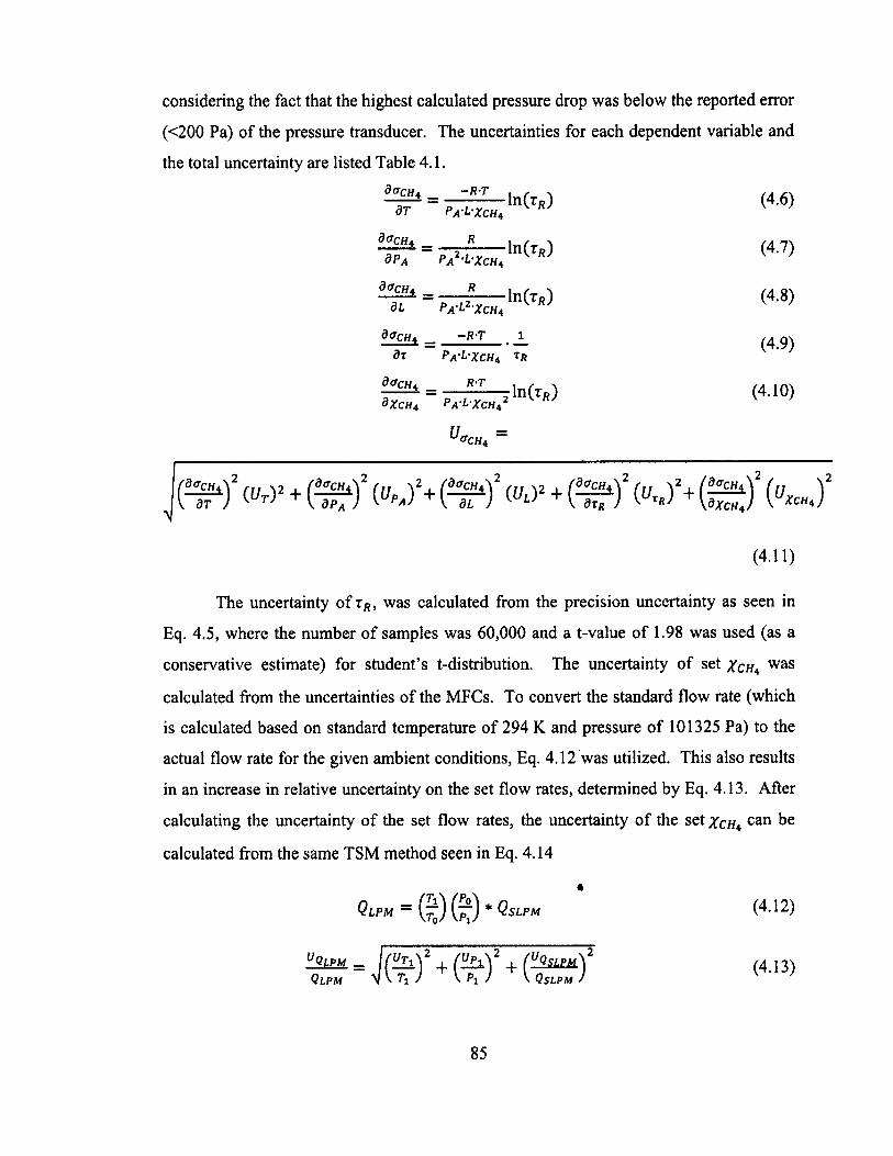
considering the fact that the highest calculated pressure drop was below the reported error

(<200 Pa) of the pressure transducer. The uncertainties for each dependent variable and

the total uncertainty are listed Table 4.1.

dT * = ~R'T ln (rR) d T P a -L-Xc h 4 V

(4.6)

d°CH* = 2 * ln(T*) d P A P a 2-L-Xc h 4

(4.7)

d f f c H 4 _ R d L P a 'L2 'X c h 4 ^

(4.8)

d a CH4 _ - R - T 1

d r P a L-X c h 4 r R(4.9)

¥ * * ■ = R'T , l n ( r R)&X c h 4 p a 'l 'X c h 4

(4.10)

U « c h 4 =

j ( ^ ) 2 + ( ^ ) 2 (»,„)’+ f m ) ! + ( ^ ) 2 k ) 2+ g ^ ) 2 K J

(4.11)

The uncertainty o f rR, was calculated from the precision uncertainty as seen in

Eq. 4.5, where the number o f samples was 60,000 and a t-value o f 1.98 was used (as a

conservative estimate) for student’s t-distribution. The uncertainty o f set X c h 4 was calculated from the uncertainties of the MFCs. To convert the standard flow rate (which

is calculated based on standard temperature o f 294 K and pressure o f 101325 Pa) to the

actual flow rate for the given ambient conditions, Eq. 4.12 was utilized. This also results

in an increase in relative uncertainty on the set flow rates, determined by Eq. 4.13. After

calculating the uncertainty o f the set flow rates, the uncertainty o f the set X c h 4 can be

calculated from the same TSM method seen in Eq. 4.14

Q l p m = ( r) ( ) * Q s l p m (4-12)

85

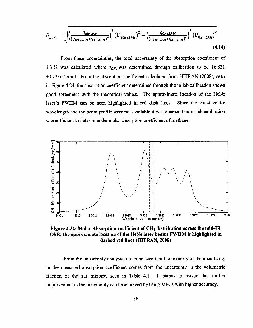
^ \(QcH4,LPM+Qair,LPM)(; Qalr.LPM2

) ( ( W m) 2 + (;(QcH4,LPM+Qalr,LPM)

QCH4,LPM

(4.14)

From these uncertainties, the total uncertainty o f the absorption coefficient of

1.3% was calculated where aCHi was determined through calibration to be 16.831

±0.223m2 /mol. From the absorption coefficient calculated from HITRAN (2008), seen

in Figure 4.24, the absorption coefficient determined through the in lab calibration shows

good agreement with the theoretical values. The approximate location of the HeNe

laser’s FWHM can be seen highlighted in red dash lines. Since the exact centre

wavelength and the beam profile were not available it was deemed that in-lab calibration

was sufficient to determine the molar absorption coefficient o f methane.

^ 351---------- ,---------- 1---------- 1---------- 1----------- 1---1—|--- 1---------- 1 i i

Figure 4.24: Molar Absorption coefficient of CH4 distribution across the mid-IR OSR; the approximate location of the HeNe laser beams FWHM is highlighted in

dashed red lines (HITRAN, 2008)

From the uncertainty analysis, it can be seen that the majority o f the uncertainty

in the measured absorption coefficient comes from the uncertainty in the volumetric

fraction o f the gas mixture, seen in Table 4.1. It stands to reason that further

improvement in the uncertainty can be achieved by using MFCs with higher accuracy.

3.391 3.3912 3.3914 3.3916 3.3918 3 392 3.3922 3.3924 3.3926 3.3928 3.393Wavelenght (micrometres)

86

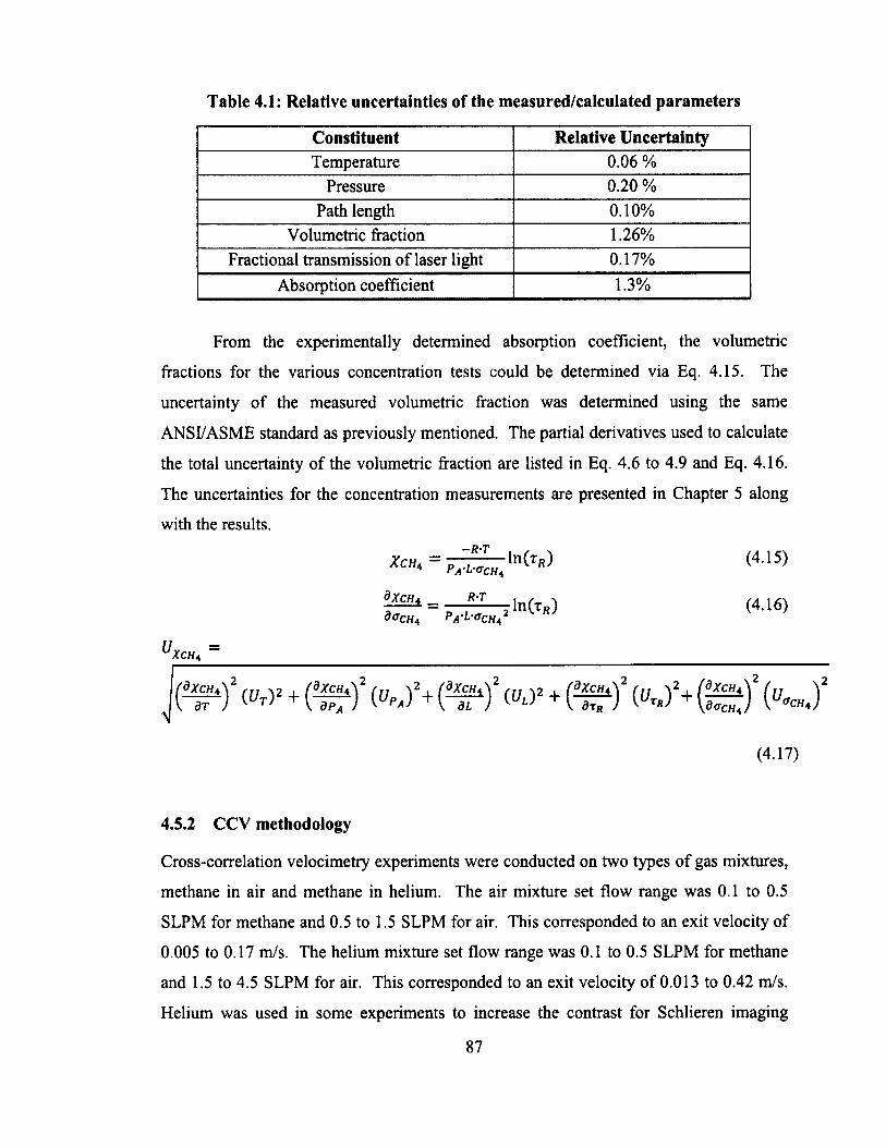
Table 4.1: Relative uncertainties of the measured/calculated parameters

Constituent Relative UncertaintyTemperature 0.06 %

Pressure 0.20 %Path length 0.10%

Volumetric fraction 1.26%Fractional transmission of laser light 0.17%

Absorption coefficient 1.3%

From the experimentally determined absorption coefficient, the volumetric

fractions for the various concentration tests could be determined via Eq. 4.15. The

uncertainty o f the measured volumetric fraction was determined using the same

ANSI/ASME standard as previously mentioned. The partial derivatives used to calculate

the total uncertainty of the volumetric fraction are listed in Eq. 4.6 to 4.9 and Eq. 4.16.

The uncertainties for the concentration measurements are presented in Chapter 5 along

with the results.

X c h ± = —~ ~ — ln (T«) (4-15)PA-L-0CH4 R

= IM' , ln(Tj;) (4.16)0<7CH4 PA'L'aCH4

XCHA

| ( ^ ) 2 (uTy + ( ^ f ) 2 {u Pi) \ ( ^ ) 2 w + ( ^ ) 2 ( u . , ) 2+ ( ^ i ) 2

(4.17)

4.5.2 CCV methodology

Cross-correlation velocimetry experiments were conducted on two types o f gas mixtures,

methane in air and methane in helium. The air mixture set flow range was 0.1 to 0.5

SLPM for methane and 0.5 to 1.5 SLPM for air. This corresponded to an exit velocity of

0.005 to 0.17 m/s. The helium mixture set flow range was 0.1 to 0.5 SLPM for methane

and 1.5 to 4.5 SLPM for air. This corresponded to an exit velocity of 0.013 to 0.42 m/s.

Helium was used in some experiments to increase the contrast for Schlieren imaging

87

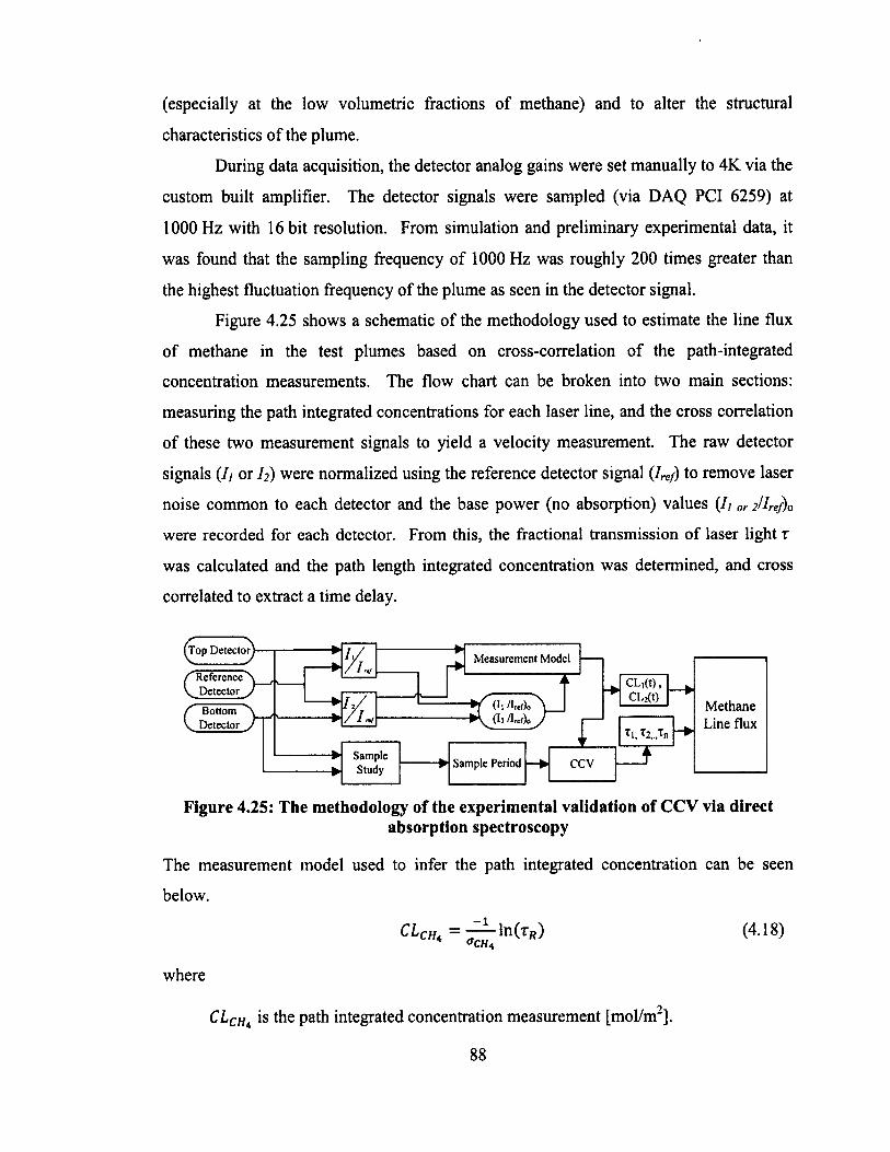
(especially at the low volumetric fractions o f methane) and to alter the structural

characteristics o f the plume.

During data acquisition, the detector analog gains were set manually to 4K via the

custom built amplifier. The detector signals were sampled (via DAQ PCI 6259) at

1000 Hz with 16 bit resolution. From simulation and preliminary experimental data, it

was found that the sampling frequency o f 1000 Hz was roughly 200 times greater than

the highest fluctuation frequency o f the plume as seen in the detector signal.

Figure 4.25 shows a schematic of the methodology used to estimate the line flux

of methane in the test plumes based on cross-correlation of the path-integrated

concentration measurements. The flow chart can be broken into two main sections:

measuring the path integrated concentrations for each laser line, and the cross correlation

of these two measurement signals to yield a velocity measurement. The raw detector

signals (// or I2) were normalized using the reference detector signal (7re/) to remove laser

noise common to each detector and the base power (no absorption) values (/; or 2//re/)0

were recorded for each detector. From this, the fractional transmission o f laser light r

was calculated and the path length integrated concentration was determined, and cross

correlated to extract a time delay.

ccvSampleStudy Sample Period

Measurement Model

M ethane Line flux

Figure 4.25: The methodology of the experimental validation of CCV via directabsorption spectroscopy

The measurement model used to infer the path integrated concentration can be seen

below.

CLch4 = ~ ln (Ti?) (4-18)4 ffCW4

where

CLCHa is the path integrated concentration measurement [mol/m2].

88

Figure 4.26 and Figure 4.27 shows an example o f the cross-correlation o f the two

time-resolved path integrated concentration signals. The dominant time lag between the

two signals occurs where Rxy is maximized, corresponding to a time delay o f 0.937

seconds (i.e. 937 samples at a sample frequency of 1000Hz). Given the fixed beam

separation distance o f 39.1 mm, the 0.937 s time delay equates to an average flow

velocity of 0.042 m/s (see Eq. 4.19).

0 .9 5

0 .9

0 8 5

0.8%s 0 7 5

0 .7

0 8 5

0.6

0 .5 5

0 -5 .

Time (s)

Figure 4.26: Example of r for Air -Methane Test

89

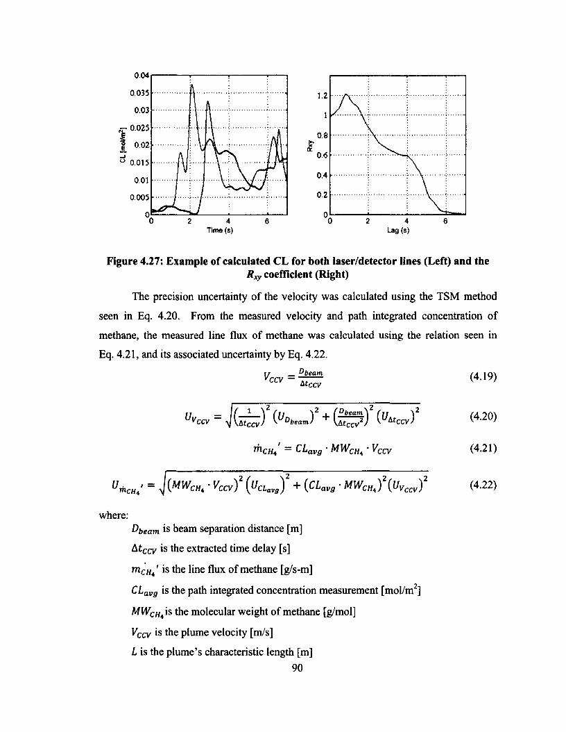
0.04

0.035

0.03

s - 0.025

0.02

° 0.015

0.01

0.005

Time (s)

0.8>»XGC

0.6

0.4

0.2

Lag (s)

Figure 4.27: Example of calculated CL for both laser/detector lines (Left) and theRxy coefficient (Right)

The precision uncertainty of the velocity was calculated using the TSM method

seen in Eq. 4.20. From the measured velocity and path integrated concentration of

methane, the measured line flux o f methane was calculated using the relation seen in

Eq. 4.21, and its associated uncertainty by Eq. 4.22.

ir ®beamVCCV ~ ------A tc cv

UVCCV= If'

m CHA CLavg • MWCha • Vccv

= J ( MWc». ■ Vccv) 2 { U c l „ S + {CLav, ■ MWc„ , ) \ u VcJ

where:Dbeam is beam separation distance [m]

Atccv is the extracted time delay [s]

m CHA is the line flux o f methane [g/s-m]

CLavg is the path integrated concentration measurement [mol/m ]

MWCh4is the molecular weight o f methane [g/mol]

VCcv is the plume velocity [m/s]

L is the plume’s characteristic length [m]90

(4.19)

(4.20)

(4.21)

(4.22)

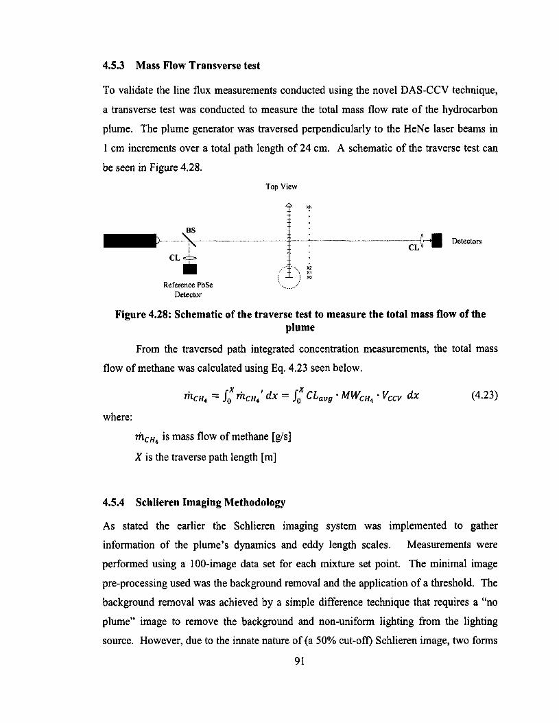
4.5.3 Mass Flow Transverse test

To validate the line flux measurements conducted using the novel DAS-CCV technique,

a transverse test was conducted to measure the total mass flow rate o f the hydrocarbon

plume. The plume generator was traversed perpendicularly to the HeNe laser beams in

1 cm increments over a total path length of 24 cm. A schematic o f the traverse test can

be seen in Figure 4.28.

Top View

r r f l Detectors

z

\ BS

> XN

CL =

1 1 f i •"'v X \ XL ; x

CL

210Reference PbSe

Detector

Figure 4.28: Schematic of the traverse test to measure the total mass flow of theplume

From the traversed path integrated concentration measurements, the total mass

flow of methane was calculated using Eq. 4.23 seen below.

rhCH4 — f0 ™-ch4 dx — fQ CLavg • MWCHt ‘ Vccv dx

rhCHi is mass flow of methane [g/s]

X is the traverse path length [m]

where:

(4.23)

4.5.4 Schlieren Imaging Methodology

As stated the earlier the Schlieren imaging system was implemented to gather

information of the plume’s dynamics and eddy length scales. Measurements were

performed using a 100-image data set for each mixture set point. The minimal image

pre-processing used was the background removal and the application o f a threshold. The

background removal was achieved by a simple difference technique that requires a “no

plume” image to remove the background and non-uniform lighting from the lighting

source. However, due to the innate nature of (a 50% cut-off) Schlieren image, two forms

91

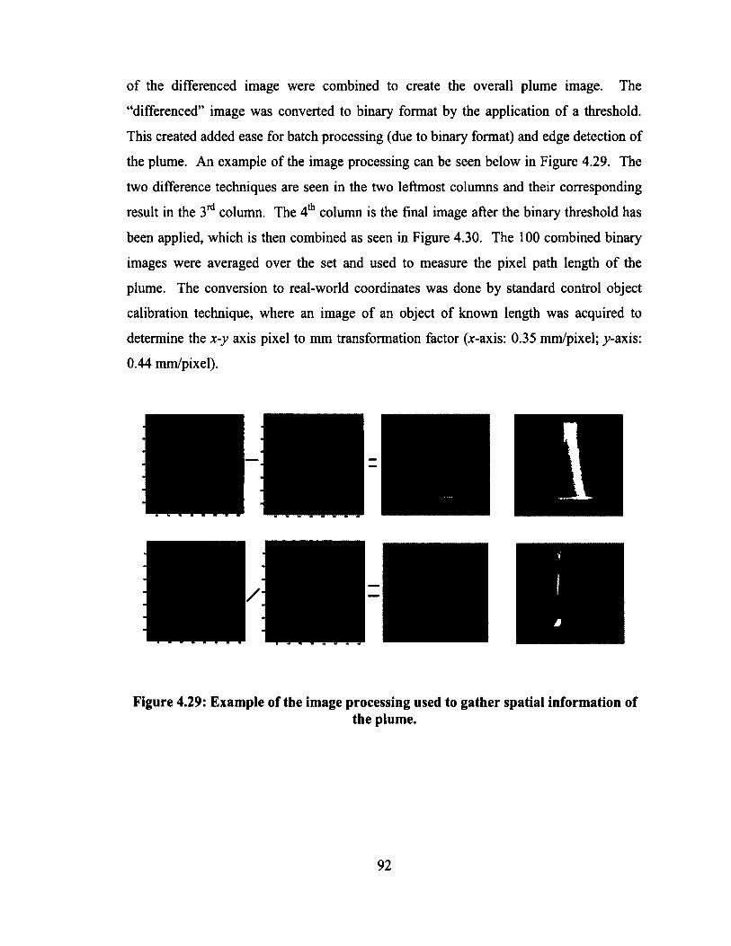
of the differenced image were combined to create the overall plume image. The

“differenced” image was converted to binary format by the application o f a threshold.

This created added ease for batch processing (due to binary format) and edge detection of

the plume. An example of the image processing can be seen below in Figure 4.29. The

two difference techniques are seen in the two leftmost columns and their corresponding

result in the 3rd column. The 4th column is the final image after the binary threshold has

been applied, which is then combined as seen in Figure 4.30. The 100 combined binary

images were averaged over the set and used to measure the pixel path length o f the

plume. The conversion to real-world coordinates was done by standard control object

calibration technique, where an image of an object o f known length was acquired to

determine the x-y axis pixel to mm transformation factor (x-axis: 0.35 mm/pixel; y-axis:

0.44 mm/pixel).

Figure 4.29: Example of the image processing used to gather spatial information ofthe plume.

92

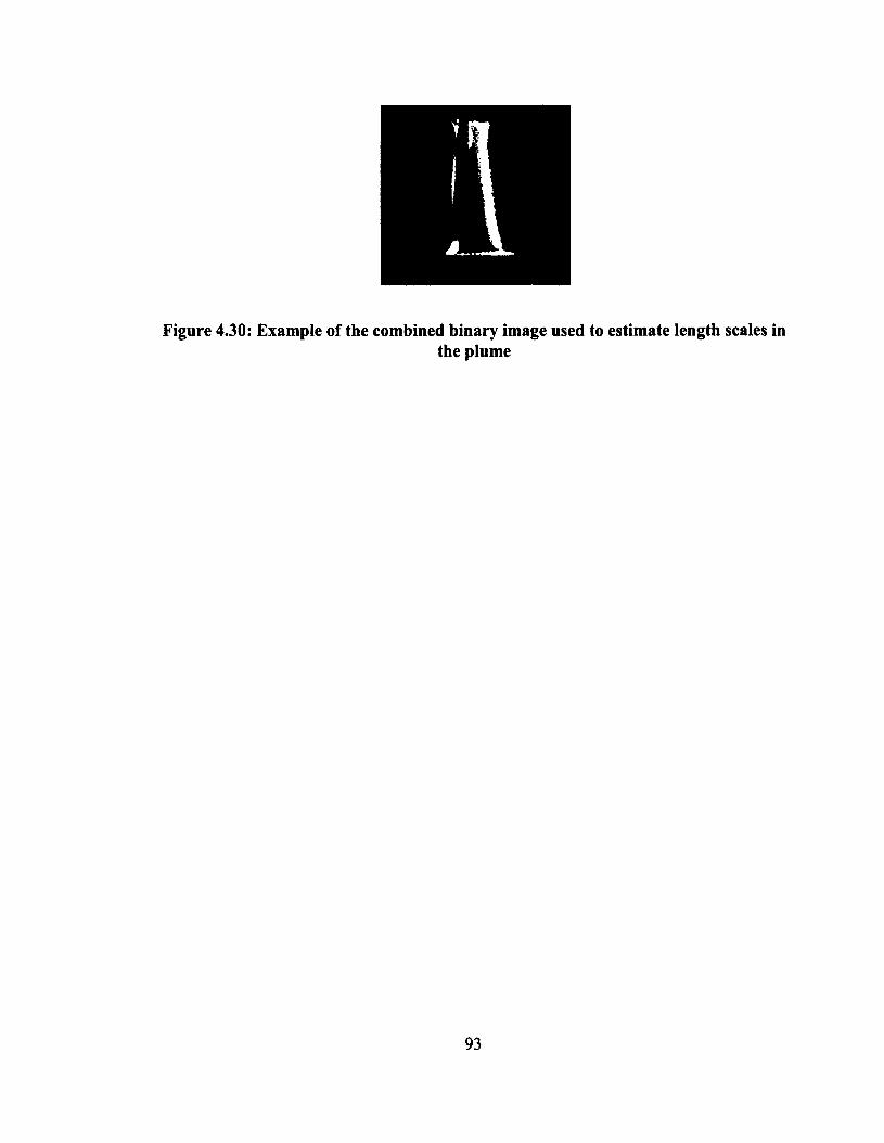
Figure 4.30: Example of the combined binary image used to estimate length scales inthe plume

93

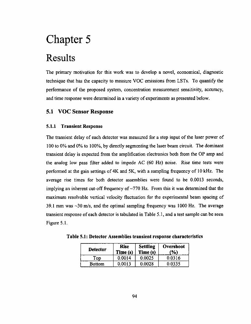
Chapter 5

ResultsThe primary motivation for this work was to develop a novel, economical, diagnostic

technique that has the capacity to measure VOC emissions from LSTs. To quantify the

performance of the proposed system, concentration measurement sensitivity, accuracy,

and time response were determined in a variety of experiments as presented below.

5.1 VOC Sensor Response

5.1.1 Transient Response

The transient delay o f each detector was measured for a step input o f the laser power of

100 to 0% and 0% to 100%, by directly segmenting the laser beam circuit. The dominant

transient delay is expected from the amplification electronics both from the OP amp and

the analog low pass filter added to impede AC (60 Hz) noise. Rise time tests were

performed at the gain settings o f 4K and 5K, with a sampling frequency o f 10 kHz. The

average rise times for both detector assemblies were found to be 0.0013 seconds,

implying an inherent cut-off frequency of -770 Hz. From this it was determined that the

maximum resolvable vertical velocity fluctuation for the experimental beam spacing of

39.1 mm was -3 0 m/s, and the optimal sampling frequency was 1000 Hz. The average

transient response o f each detector is tabulated in Table 5.1, and a test sample can be seen

Figure 5.1.

Table 5.1: Detector Assemblies transient response characteristics

Detector Rise Time (s)

Settling Time (s)

Overshoot(% )

Top 0.0014 0.0025 0.0316Bottom 0.0013 0.0028 0.0335

94

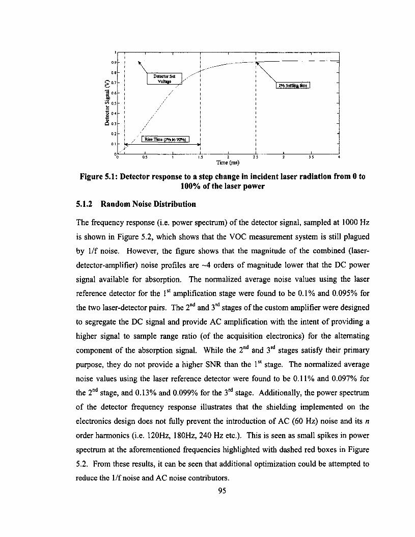
0 9

Detector Set Voltage0.7

0 6

*Si o.5

0.4

0.3

0 2

Rise Time (5% to 90%)

0 5Time (ms)

Figure 5.1: Detector response to a step change in incident laser radiation from 0 to1 0 0 % of the laser power

5.1.2 Random Noise Distribution

The frequency response (i.e. power spectrum) of the detector signal, sampled at 1000 Hz

is shown in Figure 5.2, which shows that the VOC measurement system is still plagued

by 1/f noise. However, the figure shows that the magnitude of the combined (laser-

detector-amplifier) noise profiles are ~4 orders o f magnitude lower that the DC power

signal available for absorption. The normalized average noise values using the laser

reference detector for the 1st amplification stage were found to be 0.1% and 0.095% for

the two laser-detector pairs. The 2nd and 3rd stages of the custom amplifier were designed

to segregate the DC signal and provide AC amplification with the intent o f providing a

higher signal to sample range ratio (of the acquisition electronics) for the alternating

component of the absorption signal. While the 2nd and 3rd stages satisfy their primary

purpose, they do not provide a higher SNR than the 1st stage. The normalized average

noise values using the laser reference detector were found to be 0.11% and 0.097% for

the 2nd stage, and 0.13% and 0.099% for the 3rd stage. Additionally, the power spectrum

of the detector frequency response illustrates that the shielding implemented on the

electronics design does not fully prevent the introduction o f AC (60 Hz) noise and its n

order harmonics (i.e. 120Hz, 180Hz, 240 Hz etc.). This is seen as small spikes in power

spectrum at the aforementioned frequencies highlighted with dashed red boxes in Figure

5.2. From these results, it can be seen that additional optimization could be attempted to

reduce the 1/f noise and AC noise contributors.

95

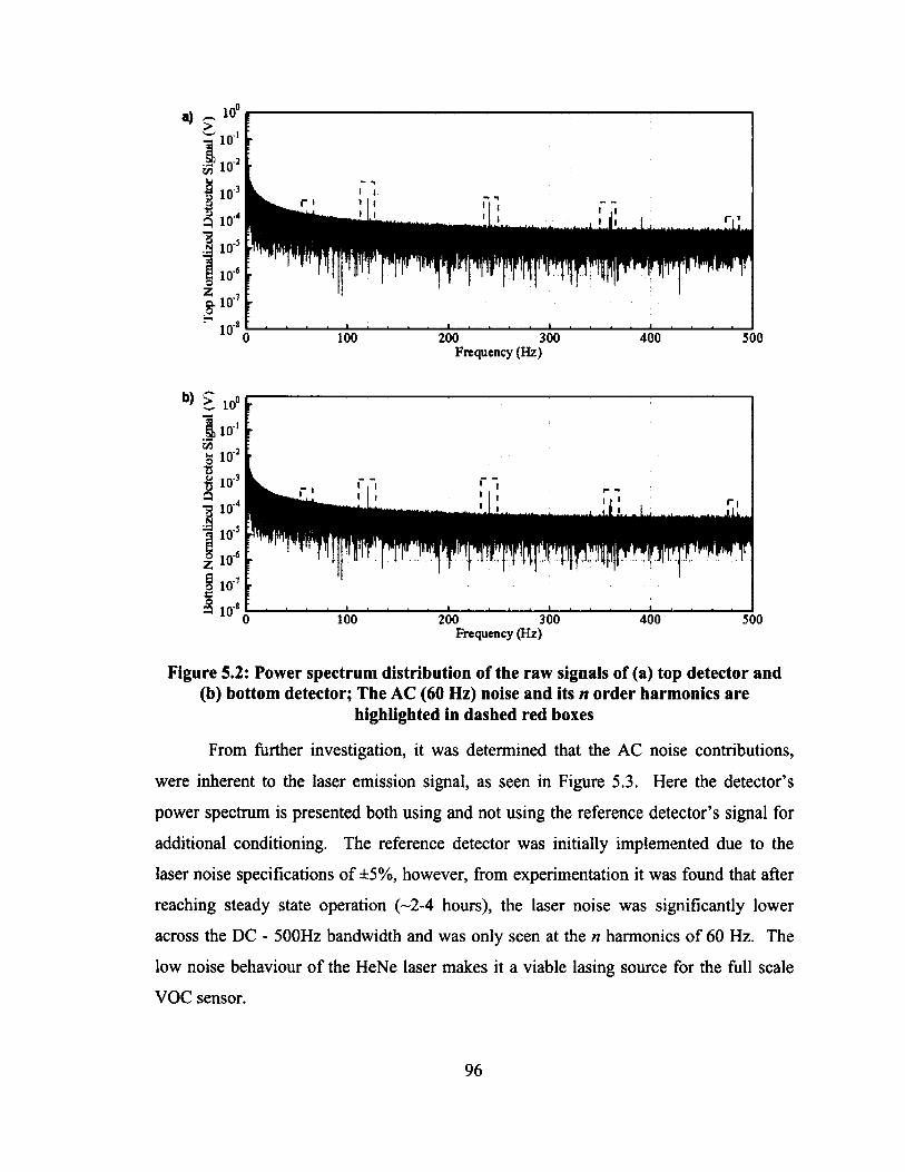
10

1(T 100 200 300Frequency (Hz)

400 500

b) > 10°

10" r

100 200 300Frequency (Hz)

400 300

Figure 5.2: Power spectrum distribution of the raw signals of (a) top detector and (b) bottom detector; The AC (60 Hz) noise and its n order harmonics are

highlighted in dashed red boxes

From further investigation, it was determined that the AC noise contributions,

were inherent to the laser emission signal, as seen in Figure 5.3. Here the detector’s

power spectrum is presented both using and not using the reference detector’s signal for

additional conditioning. The reference detector was initially implemented due to the

laser noise specifications o f ±5%, however, from experimentation it was found that after

reaching steady state operation (-2-4 hours), the laser noise was significantly lower

across the DC - 500Hz bandwidth and was only seen at the n harmonics o f 60 Hz. The

low noise behaviour o f the HeNe laser makes it a viable lasing source for the full scale

VOC sensor.

96

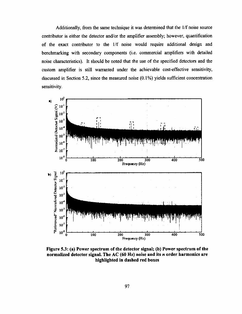
Additionally, from the same technique it was determined that the 1/f noise source

contributor is either the detector and/or the amplifier assembly; however, quantification

of the exact contributor to the 1/f noise would require additional design and

benchmarking with secondary components (i.e. commercial amplifiers with detailed

noise characteristics). It should be noted that the use o f the specified detectors and the

custom amplifier is still warranted under the achievable cost-effective sensitivity,

discussed in Section 5.2, since the measured noise (0.1%) yields sufficient concentration

sensitivity.

«)

» I 10

200 300Frequency (Hz)

200 300Frequency (Hz)

500

10 -

400 500

Figure 5.3: (a) Power spectrum of the detector signal; (b) Power spectrum of the normalized detector signal. The AC (60 Hz) noise and its n order harmonics are

highlighted in dashed red boxes

97

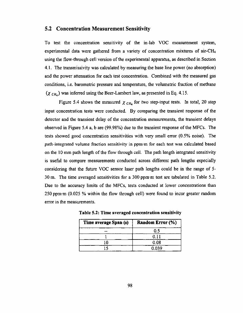
5.2 Concentration Measurement Sensitivity

To test the concentration sensitivity o f the in-lab VOC measurement system,

experimental data were gathered from a variety of concentration mixtures o f air-CFU

using the flow-through cell version o f the experimental apparatus, as described in Section

4.1. The transmissivity was calculated by measuring the base line power (no absorption)

and the power attenuation for each test concentration. Combined with the measured gas

conditions, i.e. barometric pressure and temperature, the volumetric fraction of methane

(X chJ was inferred using the Beer-Lambert law, as presented in Eq. 4.15.

Figure 5.4 shows the measured x ch4 f°r two step-input tests. In total, 20 step

input concentration tests were conducted. By comparing the transient response o f the

detector and the transient delay o f the concentration measurements, the transient delays

observed in Figure 5.4 a, b are (99.98%) due to the transient response o f the MFCs. The

tests showed good concentration sensitivities with very small error (0.5% noise). The

path-integrated volume fraction sensitivity in ppm-m for each test was calculated based

on the 10 mm path length of the flow through cell. The path length integrated sensitivity

is useful to compare measurements conducted across different path lengths especially

considering that the future VOC sensor laser path lengths could be in the range o f 5-

30 m. The time averaged sensitivities for a 300 ppm-m test are tabulated in Table 5.2.

Due to the accuracy limits of the MFCs, tests conducted at lower concentrations than

250 ppm-m (0.025 % within the flow through cell) were found to incur greater random

error in the measurements.

Table 5.2: Time averaged concentration sensitivity

Time average Span (s) Random Error (%)

— 0.51 0.11

10 0.0815 0.039

98

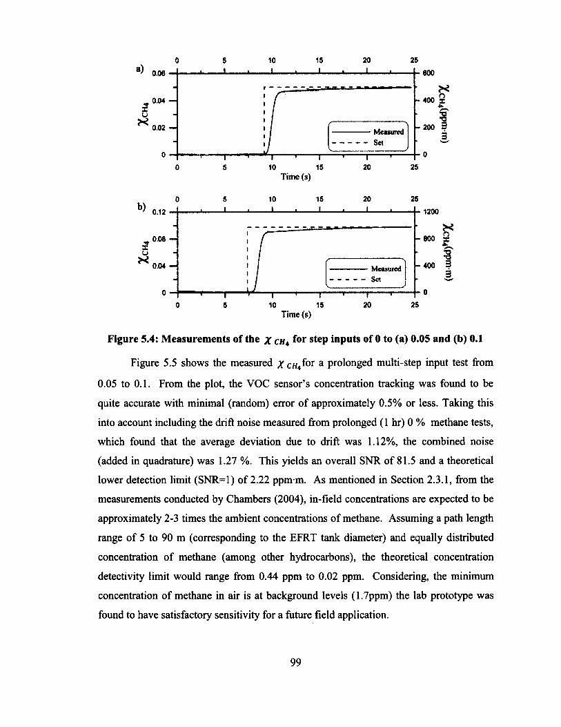
a) 0.06

0.04 —

10X

15X

20X

25

0.02 — ;-

! - - Set

i « r10 15

Time (s)

b)

3u

10 15

T "20

20

^2400 X

- 200

25

2512000.12

6000.08

4000.04 MeasuredSet

020 250 5 10 15

£

Time (s)

Figure 5.4: Measurements of the x ch4 for step inputs of 0 to (a) 0.05 and (b) 0.1

Figure 5.5 shows the measured x ch4f°r a prolonged multi-step input test from

0.05 to 0.1. From the plot, the VOC sensor’s concentration tracking was found to be

quite accurate with minimal (random) error o f approximately 0.5% or less. Taking this

into account including the drift noise measured from prolonged (1 hr) 0 % methane tests,

which found that the average deviation due to drift was 1.12%, the combined noise

(added in quadrature) was 1.27 %. This yields an overall SNR of 81.5 and a theoretical

lower detection limit (SNR=1) o f 2.22 ppm-m. As mentioned in Section 2.3.1, from the

measurements conducted by Chambers (2004), in-field concentrations are expected to be

approximately 2-3 times the ambient concentrations o f methane. Assuming a path length

range o f 5 to 90 m (corresponding to the EFRT tank diameter) and equally distributed

concentration of methane (among other hydrocarbons), the theoretical concentration

detectivity limit would range from 0.44 ppm to 0.02 ppm. Considering, the minimum

concentration o f methane in air is at background levels (1.7ppm) the lab prototype was

found to have satisfactory sensitivity for a future field application.

99

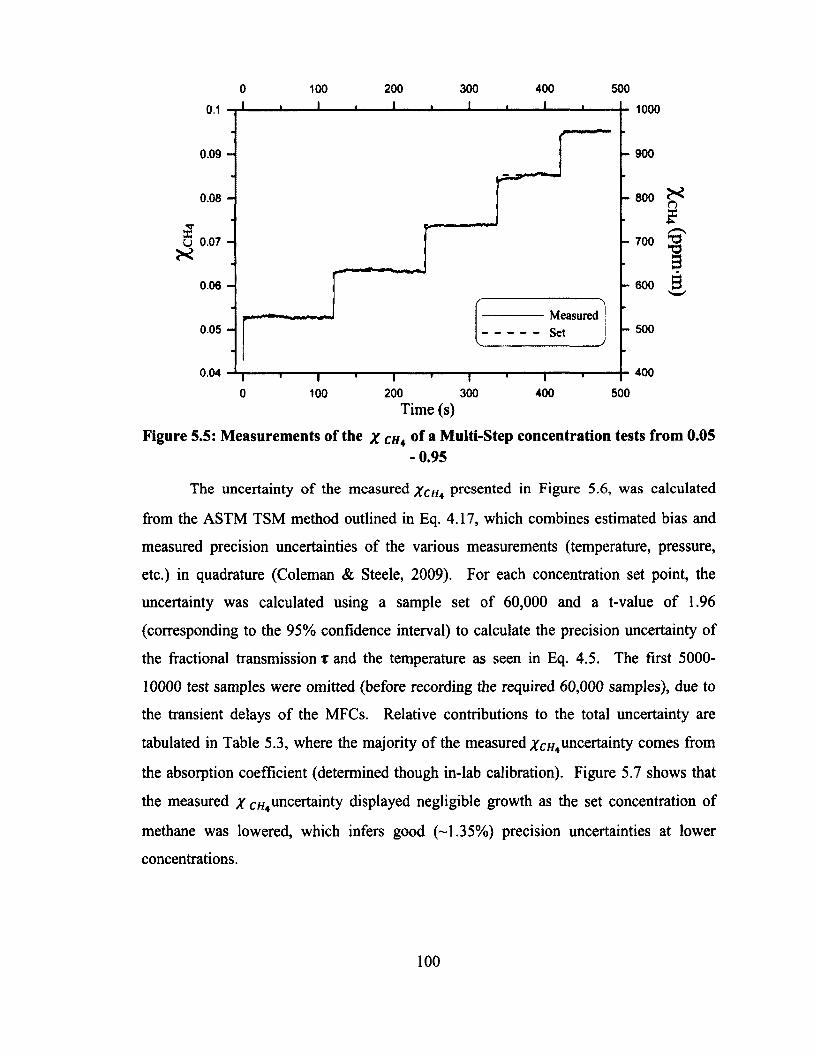
100 200 300 400 50010000.1

- 9000.09

- 8000.08 -

- 700U 0.07 -

- 6000.06 -

Measured j Set - 5000.05 -

4000.04

400200 300 5000 100

133 3

Time (s)

Figure 5.5: Measurements of the x c h 4 of a Multi-Step concentration tests from 0.05-0.95

The uncertainty of the measured X c h 4 presented in Figure 5.6, was calculated

from the ASTM TSM method outlined in Eq. 4.17, which combines estimated bias and

measured precision uncertainties o f the various measurements (temperature, pressure,

etc.) in quadrature (Coleman & Steele, 2009). For each concentration set point, the

uncertainty was calculated using a sample set o f 60,000 and a t-value o f 1.96

(corresponding to the 95% confidence interval) to calculate the precision uncertainty of

the fractional transmission x and the temperature as seen in Eq. 4.5. The first 5000-

10000 test samples were omitted (before recording the required 60,000 samples), due to

the transient delays o f the MFCs. Relative contributions to the total uncertainty are

tabulated in Table 5.3, where the majority o f the measured X c h 4uncertainty comes from

the absorption coefficient (determined though in-lab calibration). Figure 5.7 shows that

the measured x c h 4uncertainty displayed negligible growth as the set concentration of

methane was lowered, which infers good (-1.35%) precision uncertainties at lower

concentrations.

100

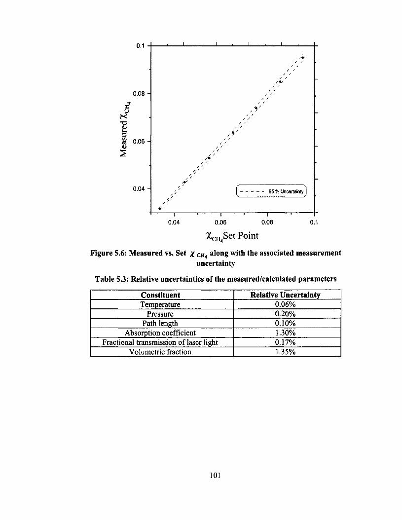
0.08

IuXT3IS3 0.06<L>

S

0.04

1

Figure 5.6: Measured vs. Set x cha along with the associated measurementuncertainty

Table 5.3: Relative uncertainties of the measured/calculated parameters

Constituent Relative UncertaintyTemperature 0.06%

Pressure 0.20%Path length 0.10%

Absorption coefficient 1.30%Fractional transmission of laser light 0.17%

Volumetric fraction 1.35%

XCH.Set Point

101

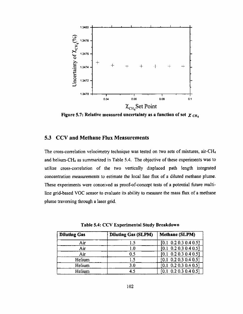
1.3480

s®O'-® \ 1.3478 -

IU

o£*

1.3476 -

c'30)oc

D

£- 1.3474 -

1.3472 -

1.3470

XCH4Set PointFigure 5.7: Relative measured uncertainty as a function of set x ch4

5.3 CCV and Methane Flux Measurements

The cross-correlation velocimetry technique was tested on two sets o f mixtures, air-CH4

and helium-CH4 as summarized in Table 5.4. The objective of these experiments was to

utilize cross-correlation of the two vertically displaced path length integrated

concentration measurements to estimate the local line flux o f a diluted methane plume.

These experiments were conceived as proof-of-concept tests o f a potential future multi-

line grid-based VOC sensor to evaluate its ability to measure the mass flux of a methane

plume traversing through a laser grid.

Table 5.4: CCV Experimental Study Breakdown

Diluting Gas Diluting Gas (SLPM) Methane (SLPM)

Air 1.5 ro.l 0.2 0.3 0.4 0.51Air 1.0 [0.1 0.2 0.3 0.4 0.5]Air 0.5 ro.l 0.2 0.3 0.4 0.51

Helium 1.5 [0.1 0.2 0.3 0.4 0.51Helium 3.0 [0.1 0.2 0.3 0.4 0.51Helium 4.5 [0.1 0.2 0.3 0.4 0.51

102

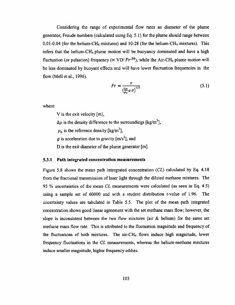
Considering the range of experimental flow rates an diameter o f the plume

generator, Froude numbers (calculated using Eq. 5.1) for the plume should range between

0.01-0.04 (for the helium-CFLj mixtures) and 10-28 (for the helium-CFLt mixtures). This

infers that the helium-CFL* plume motion will be buoyancy dominated and have a high

fluctuation (or pulsation) frequency (oc VD/ F r 38), while the Air-CH4 plume motion will

be less dominated by buoyant effects and will have lower fluctuation frequencies in the

flow (Mell et al., 1996).

where:

V is the exit velocity [m],

Ap is the density difference to the surroundings [kg/m3],

p0 is the reference density [kg/m3],

g is acceleration due to gravity [m/s ], and

D is the exit diameter o f the plume generator [m].

5.3.1 Path integrated concentration measurements

Figure 5.8 shows the mean path intergrated concentration (CL) calculated by Eq. 4.18

from the fractional transmission of laser light through the diluted methane mixtures. The

95 % uncertainties of the mean CL measurements were calculated (as seen in Eq. 4.5)

using a sample set of 60000 and with a student distribution t-value of 1.96. The

uncertainty values are tabulated in Table 5.5. The plot o f the mean path integrated

concentration shows good linear agreement with the set methane mass flow; however, the

slope is inconsistent between the two flow mixtures (air & helium) for the same set

methane mass flow rate. This is attributed to the fluctuation magnitude and frequency of

the fluctuations of both mixtures. The air-CH4 flows induce high magnitude, lower

frequency fluctuations in the CL measurements, whereas the helium-methane mixtures

induce smaller magnitude, higher frequency eddies.

103

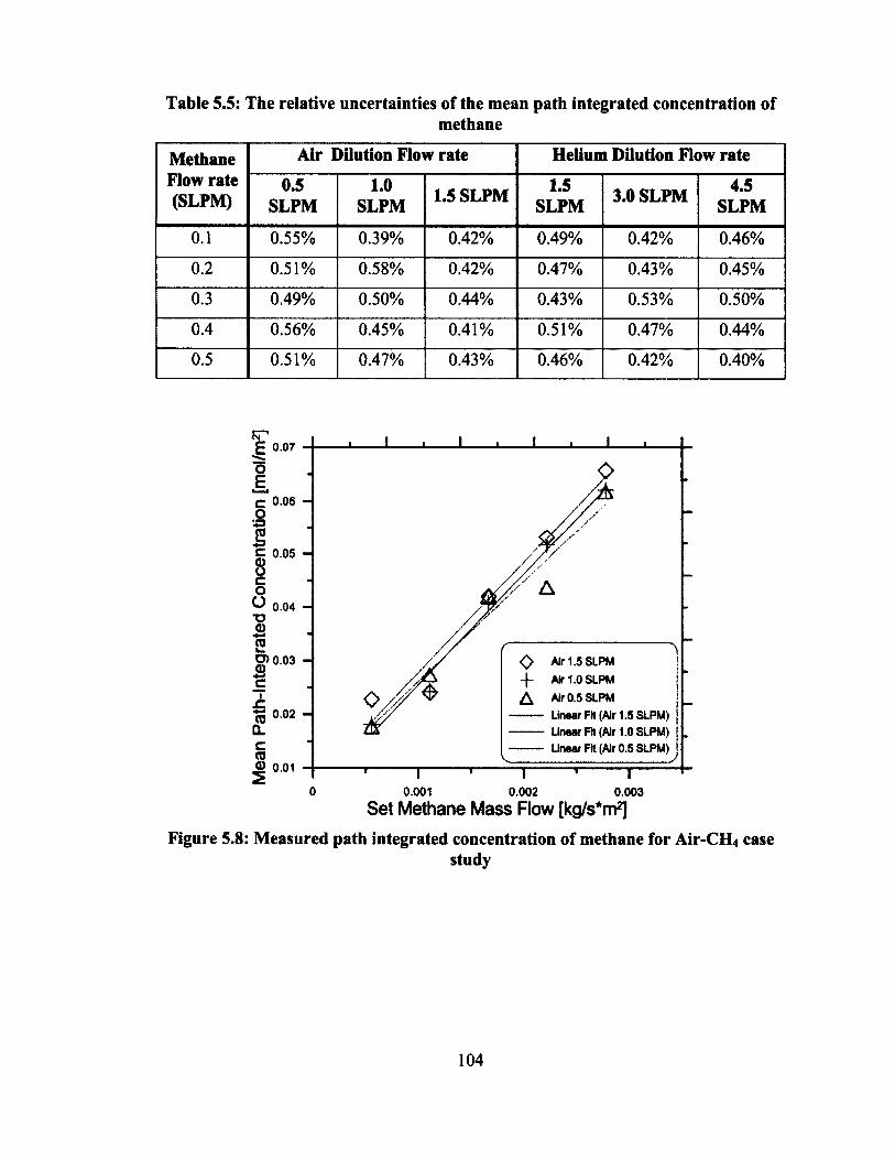
Table 5.5: The relative uncertainties of the mean path integrated concentration ofmethane

Methane Flow rate (SLPM)

Air Dilution Flow rate Helium Dilution Flow rate

0.5SLPM

1 . 0

SLPM 1.5 SLPM 1.5SLPM 3.0 SLPM 4.5

SLPM

0.1 0.55% 0.39% 0.42% 0.49% 0.42% 0.46%

0.2 0.51% 0.58% 0.42% 0.47% 0.43% 0.45%

0.3 0.49% 0.50% 0.44% 0.43% 0.53% 0.50%

0.4 0.56% 0.45% 0.41% 0.51% 0.47% 0.44%

0.5 0.51% 0.47% 0.43% 0.46% 0.42% 0.40%

£ 0.07 — I I l I — ■—x ——■ L JL.„.— .1 .........i,

O Air 1.5 SLPM-(- Air 1.0 SLPMA Air 0.5 SLPM Unear Fit (Air 1.5 SLPM) Linear Fit (Air 1.0 SLPM) Unear Fit (Air 0.5 SLPM)

0 0.001 0.002 0.003Set Methane Mass Flow [kg/s'm2]

Figure 5.8: Measured path integrated concentration of methane for Air-CH4 casestudy

104

£ 0.04

0.03

0.02 -TJ

O) O He4.5Sl.PM -f- He 3.0 SLPMA He 1.5 SLPM Linear Fit (He 4.5 SLPM) Linear Fit (He 3.0 SLPM) Unear Fit (He 1.5 SLPM)

0.01

0.001 0.002 Set Methane Mass Flow [kg/s^m2]

0.0030

Figure 5.9: Measured path integrated concentration of methane for the Helium-CH4

case study

5.3.2 CCV

As stated in Section 3.1.2, the main parameters that affect the cross correlation function

are: turbulent eddy behaviour, laser beam separation, measurement noise, sampling

frequency and sampling period. The turbulent eddy behaviour o f the plume was an

uncontrolled function o f the buoyant properties o f the set mixture flow. The laser beam

separation was kept to a minimum of 39.1 mm, based on the minimal achievable spacing

between commercially available rigid Mid-IR optical components with protective

enclosures. The measurement noise parameters were determined by the economical

amplifier design as presented in Section 5.1.2. The sampling frequency was selected

based on the transient response behaviour of the detector and amplifiers, presented in

Section 5.1 where the cut-off frequency was determined. The cut-off frequency

determines the optimal point where a lower frequency results in a loss o f information and

a higher frequency results in no gain o f information for the additional resources required

(i.e. buffer memory, computational effort etc..).

105

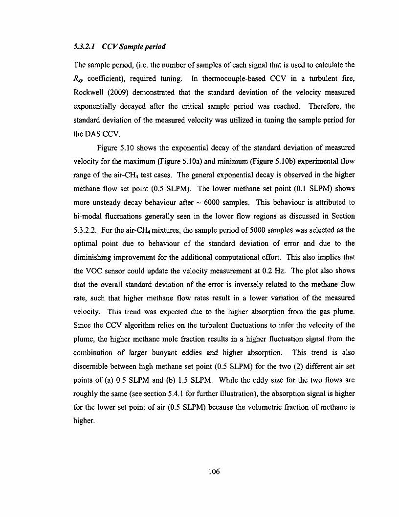
5.3.2.1 CCV Sample period

The sample period, (i.e. the number of samples o f each signal that is used to calculate the

Rxy coefficient), required tuning. In thermocouple-based CCV in a turbulent fire,

Rockwell (2009) demonstrated that the standard deviation o f the velocity measured

exponentially decayed after the critical sample period was reached. Therefore, the

standard deviation o f the measured velocity was utilized in tuning the sample period for

the DAS CCV.

Figure 5.10 shows the exponential decay of the standard deviation of measured

velocity for the maximum (Figure 5.10a) and minimum (Figure 5.10b) experimental flow

range of the air-CH4 test cases. The general exponential decay is observed in the higher

methane flow set point (0.5 SLPM). The lower methane set point (0.1 SLPM) shows

more unsteady decay behaviour after ~ 6000 samples. This behaviour is attributed to

bi-modal fluctuations generally seen in the lower flow regions as discussed in Section

5.3.2.2. For the air-CFLmixtures, the sample period o f 5000 samples was selected as the

optimal point due to behaviour o f the standard deviation o f error and due to the

diminishing improvement for the additional computational effort. This also implies that

the VOC sensor could update the velocity measurement at 0.2 Hz. The plot also shows

that the overall standard deviation o f the error is inversely related to the methane flow

rate, such that higher methane flow rates result in a lower variation of the measured

velocity. This trend was expected due to the higher absorption from the gas plume.

Since the CCV algorithm relies on the turbulent fluctuations to infer the velocity o f the

plume, the higher methane mole fraction results in a higher fluctuation signal from the

combination o f larger buoyant eddies and higher absorption. This trend is also

discernible between high methane set point (0.5 SLPM) for the two (2) different air set

points o f (a) 0.5 SLPM and (b) 1.5 SLPM. While the eddy size for the two flows are

roughly the same (see section 5.4.1 for further illustration), the absorption signal is higher

for the lower set point of air (0.5 SLPM) because the volumetric fraction of methane is

higher.

106

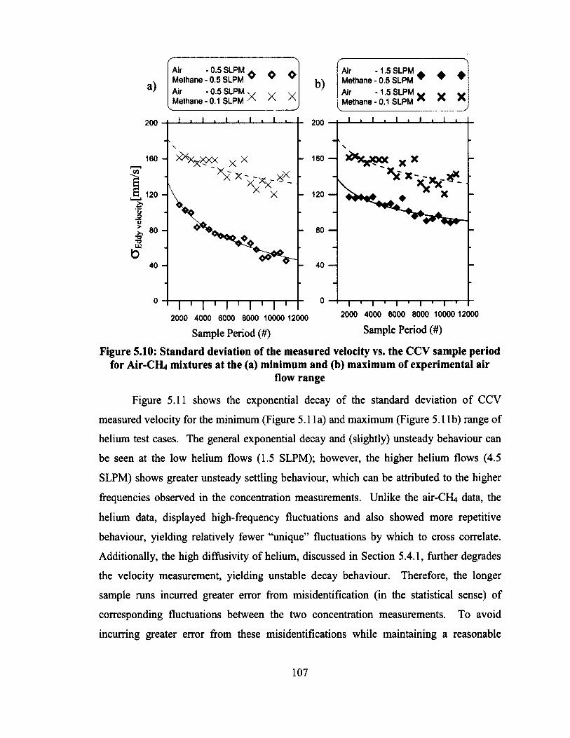
a)Air - 0.5 SLPMMethane - 0.5 SLPM Air - 0.5 SLPMMethane - 0.1 SLPM

❖ o

X X

❖

Xb)

Air -1.5 SLPMMethane - 0.5 SLPM Air -1.5 SLPM, Methane - 0.1 SLPM '

♦ ♦

X X

160 —160 -

120 -

I 1....1... - i -T - - r - T- - r - r2000 4000 6000 8000 10000 12000

Sample Period (#)

1 I i I 1 I 1 I r2000 4000 6000 8000 10000 12000

Sample Period (#)

Figure 5.10: Standard deviation of the measured velocity vs. the CCV sample period for Air-CH4 mixtures at the (a) minimum and (b) maximum of experimental air

flow range

Figure 5.11 shows the exponential decay of the standard deviation o f CCV

measured velocity for the minimum (Figure 5.1 la) and maximum (Figure 5.1 lb) range o f

helium test cases. The general exponential decay and (slightly) unsteady behaviour can

be seen at the low helium flows (1.5 SLPM); however, the higher helium flows (4.5

SLPM) shows greater unsteady settling behaviour, which can be attributed to the higher

frequencies observed in the concentration measurements. Unlike the air-CFL data, the

helium data, displayed high-frequency fluctuations and also showed more repetitive

behaviour, yielding relatively fewer “unique” fluctuations by which to cross correlate.

Additionally, the high diffusivity of helium, discussed in Section 5.4.1, further degrades

the velocity measurement, yielding unstable decay behaviour. Therefore, the longer

sample runs incurred greater error from misidentification (in the statistical sense) of

corresponding fluctuations between the two concentration measurements. To avoid

incurring greater error from these misidentifications while maintaining a reasonable

107

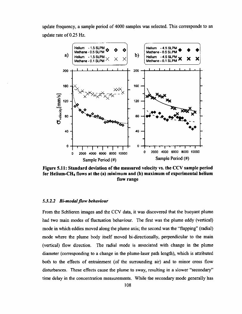
update frequency, a sample period o f 4000 samples was selected. This corresponds to an

update rate o f 0.25 Hz.

a)

Helium -1.5 SLPM A A AMethane - 0.5 SLPM ” v vHelium -1.5 SLPM v v vMethane-0.1 SLPM A A A

b)

Helium • 4.5 SLPM Methane - 0.5 SLPM Helium -4.5 SLPM Methane - 0.1 SLPM

♦ ♦ ♦

X X X

160 -

- -120 —120 -

i ; i | r | "».... | .... i.....

0 2000 4000 6000 8000 10000

Sample Period (#)

' I 1 I ' I ' I 1 I0 2000 4000 6000 8000 10000

Sample Period (#)

Figure 5.11: Standard deviation of the measured velocity vs. the CCV sample period for Helium-CH4 flows at the (a) minimum and (b) maximum of experimental helium

flow range

S. 3.2.2 Bi-modal flow behaviour

From the Schlieren images and the CCV data, it was discovered that the buoyant plume

had two main modes o f fluctuation behaviour. The first was the plume eddy (vertical)

mode in which eddies moved along the plume axis; the second was the “flapping” (radial)

mode where the plume body itself moved bi-directionally, perpendicular to the main

(vertical) flow direction. The radial mode is associated with change in the plume

diameter (corresponding to a change in the plume-laser path length), which is attributed

both to the effects o f entrainment (of the surrounding air) and to minor cross flow

disturbances. These effects cause the plume to sway, resulting in a slower “secondary”

time delay in the concentration measurements. While the secondary mode generally has108

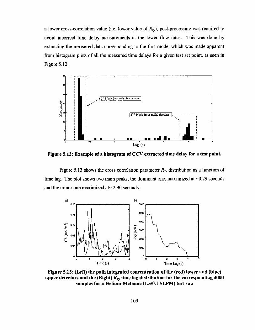
a lower cross-correlation value (i.e. lower value o f Rxy), post-processing was required to

avoid incorrect time delay measurements at the lower flow rates. This was done by

extracting the measured data corresponding to the first mode, which was made apparent

from histogram plots o f all the measured time delays for a given test set point, as seen in

Figure 5.12.

a "I 2 15 £

1** Mode from eddy fluctuations

12 Mode from radial flapping

d I 1Lag (s)

Figure 5.12: Example of a histogram of CCV extracted time delay for a test point.

Figure 5.13 shows the cross correlation parameter/?^ distribution as a function o f

time lag. The plot shows two main peaks, the dominant one, maximized at -0.29 seconds

and the minor one maximized a t- 2.90 seconds.

a) b)0.20 6000

50000.16

4000

"e 012IOE3 0.08

d

& 3000

2000

0.041000

0 1 2Time (s)

3 4

Time Lag (s)

Figure 5.13: (Left) the path integrated concentration of the (red) lower and (blue) upper detectors and the (Right) Rxy time lag distribution for the corresponding 4000

samples for a Helium-Methane (1.5/0.1 SLPM) test run

109

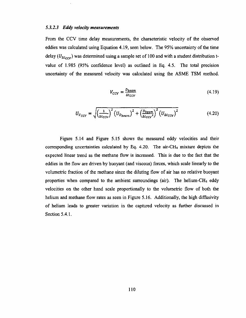
5.3.2.3 Eddy velocity measurements

From the CCV time delay measurements, the characteristic velocity o f the observed

eddies was calculated using Equation 4.19, seen below. The 95% uncertainty o f the time

delay (U^tccv) was determined using a sample set o f 100 and with a student distribution t-

value of 1.985 (95% confidence level) as outlined in Eq. 4.5. The total precision

uncertainty o f the measured velocity was calculated using the ASME TSM method.

( 4 1 9 )

^ (4.20)

Figure 5.14 and Figure 5.15 shows the measured eddy velocities and their

corresponding uncertainties calculated by Eq. 4.20. The air-CH4 mixture depicts the

expected linear trend as the methane flow is increased. This is due to the fact that the

eddies in the flow are driven by buoyant (and viscous) forces, which scale linearly to the

volumetric fraction of the methane since the diluting flow of air has no relative buoyant

properties when compared to the ambient surroundings (air). The helium-CH4 eddy

velocities on the other hand scale proportionally to the volumetric flow of both the

helium and methane flow rates as seen in Figure 5.16. Additionally, the high diffusivity

of helium leads to greater variation in the captured velocity as further discussed in

Section 5.4.1.

110

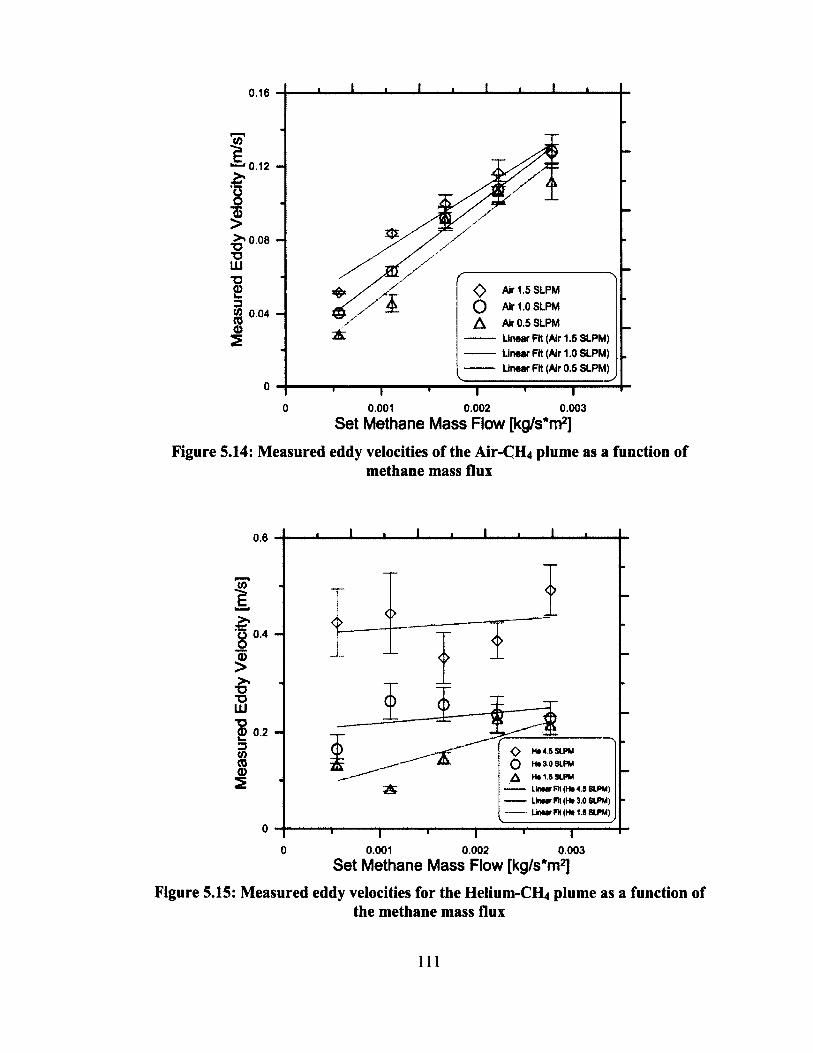
0.16

u>

&50)>>»0.08 -TJ LUTJ£□w 0.04 - \

❖ Air 1.5 SLPM Air 1.0 SLPM Air 0.5 SLPM Linear Pit (Air 1.5 SLPM) Linear Fit (Air 1.0 SLPM) Unear Fit (Air 0.5 SLPM)

0.001— r ~0.002

T I0.003

Set Methane Mass Flow [kg/s^m2]Figure 5.14: Measured eddy velocities of the Air-CH4 plume as a function of

methane mass flux

0.6

( f t

E,

f 0'"

-&IS"S 0.23( f t

3

O He 4.5 SLPM O He 3.0 SLPM

He 15 SLPM■----- Linear Rt (He 4.5 SLPM) Unaar Pit (Ha 3.0 SLPM)

Linear FH (He 15 SLPM)

T T T T0 0.001 0.002 0.003

Set Methane Mass Flow [kg/s*m2]Figure 5.15: Measured eddy velocities for the Helium-CH4 plume as a function of

the methane mass flux

111

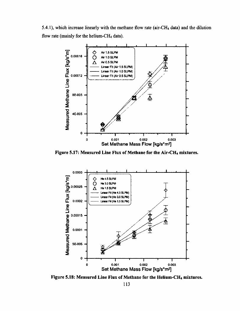
5.4.1), which increase linearly with the methane flow rate (air-CH4 data) and the dilution

flow rate (mainly for the helium-CFLt data).

E0.00016

1X_3LL 0.00012a>c

©§ 8E-OQ5 -x;a>5

4E-005D(A(0©2

OoA

_L

Air 1.5 SLPM Air 1.0 SLPM Air 0.5 SLPM Linear Fit (Air 1.5 SLPM) Linear Fit (Air 1.0 SLPM) Linear Fit (Air 0.5 SLPM)

T T1----------1---------- f-0.001 0.002 0.003

Set Methane Mass Flow [kg /s^2]Figure 5.17: Measured Line Flux of Methane for the Air-CH4 mixtures.

0.0003

«CO

■Q) 0.00025 £ .XZ3

LL 0.00020)C3© 0.00015 - c © sz©2 0.0001 H

gjj 5E-005 -n ©2

O He 4,5 SLPMO He 3.0 SLPMA He 1.5 SLPM

Linear Fit (He 4.5 SLPM) Linear Fit (He 3.0 SLPM) Linear Fit (He 1.5 SLPM)

1 1 1 1 1 1-------0 0.001 0.002 0.003

Set Methane Mass Flow [kg/s'm2]Figure 5.18: Measured Line Flux of Methane for the Helium-CIL mixtures.

113

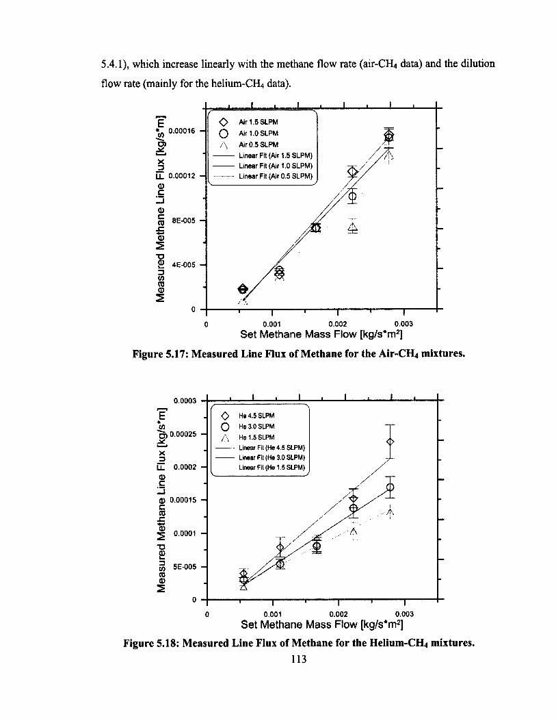
5.4.1), which increase linearly with the methane flow rate (air-CH4 data) and the dilution

flow rate (mainly for the helium-CFLt data).

E0.00016

X3

0.00012 -

OoA

Air 1.5 SLPM Air 1.0 SLPM Air 0.5 SLPM Linear Fit (Air 1.5 SLPM) Linear Fit (Air 1.0 SLPM) Linear Fit (Air 0.5 SLPM)

©c

©Cco£©

TJ©

8E-005

£ 4E-005 -3V)CO©

0.001 0.002 0.003Set Methane Mass Flow [kg/s*m2]

Figure 5.17: Measured Line Flux of Methane for the Air-CIL mixtures.

0.0003

*V)O) 0.00025 ■X,X3

LL 0.0002©c

0) 0.00015 cCO

JZ© 0.0001

\0 He 4.5 SLPM

0 He 3.0 SLPM

A He 1.5 SLPMLinear Fil (He 4.5 SLPM)Linear Fit (He 3.0 SLPM)Linear Fit (He 1.5 SLPM)

V y

5E-005

0.001 0.002 0.003Set Methane Mass Flow [kg/s*m2]

Figure 5.18: Measured Line Flux of Methane for the Helium-CIL mixtures.113

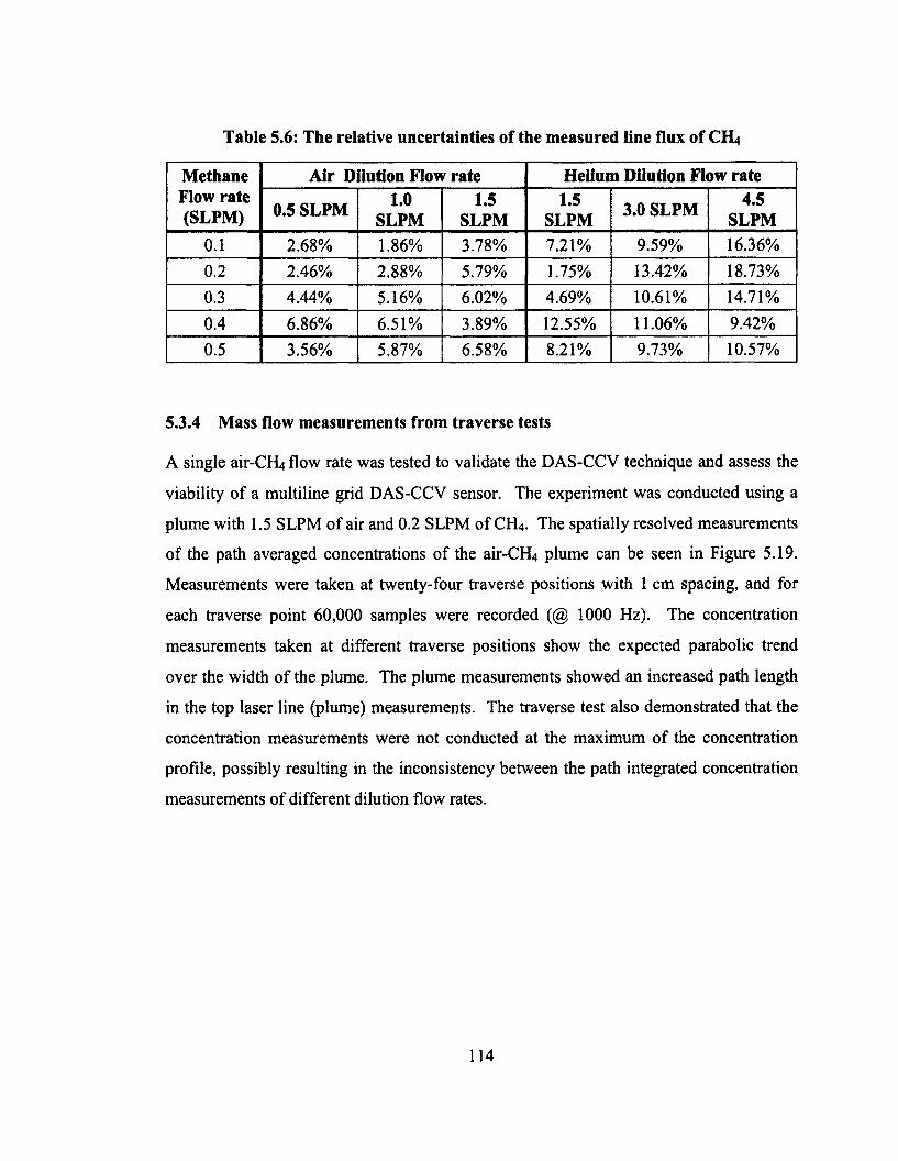
Table 5.6: The relative uncertainties of the measured line flux of CH4



0.5 SLPM 1.0SLPM

1.5SLPM

1.5SLPM 3.0 SLPM 4.5

SLPM0.1 2.68% 1.86% 3.78% 7.21% 9.59% 16.36%0.2 2.46% 2.88% 5.79% 1.75% 13.42% 18.73%0.3 4.44% 5.16% 6.02% 4.69% 10.61% 14.71%

0.4 6.86% 6.51% 3.89% 12.55% 11.06% 9.42%

0.5 3.56% 5.87% 6.58% 8.21% 9.73% 10.57%

5.3.4 Mass flow measurements from traverse tests

A single air-CH4 flow rate was tested to validate the DAS-CCV technique and assess the

viability o f a multiline grid DAS-CCV sensor. The experiment was conducted using a

plume with 1.5 SLPM of air and 0.2 SLPM of CH4. The spatially resolved measurements

of the path averaged concentrations o f the air-CH4 plume can be seen in Figure 5.19.

Measurements were taken at twenty-four traverse positions with 1 cm spacing, and for

each traverse point 60,000 samples were recorded (@ 1000 Hz). The concentration

measurements taken at different traverse positions show the expected parabolic trend

over the width o f the plume. The plume measurements showed an increased path length

in the top laser line (plume) measurements. The traverse test also demonstrated that the

concentration measurements were not conducted at the maximum of the concentration

profile, possibly resulting in the inconsistency between the path integrated concentration

measurements of different dilution flow rates.

114

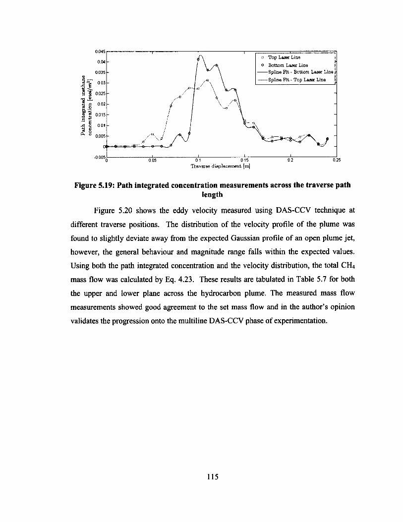
0.045o Top Laser Line

° Bottom Laser Line Spline Fit - Bottom Laser Line

Spline Fit - Top Laser Line

004

0.035

0 03I-0'

0.025

0.005

0 2501 015Traverse displacement [mj

005

Figure 5.19: Path integrated concentration measurements across the traverse pathlength

Figure 5.20 shows the eddy velocity measured using DAS-CCV technique at

different traverse positions. The distribution o f the velocity profile o f the plume was

found to slightly deviate away from the expected Gaussian profile o f an open plume jet,

however, the general behaviour and magnitude range falls within the expected values.

Using both the path integrated concentration and the velocity distribution, the total CH4

mass flow was calculated by Eq. 4.23. These results are tabulated in Table 5.7 for both

the upper and lower plane across the hydrocarbon plume. The measured mass flow

measurements showed good agreement to the set mass flow and in the author’s opinion

validates the progression onto the multiline DAS-CCV phase of experimentation.

115

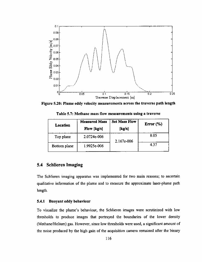
0.09

0.08

0.07

-S’o 0.06

> 0 05

3? 0 M

0.02

0.01

0.250.1 0.15Tiaverse Displacem ent [m]

0 0 5

Figure 5.20: Plume eddy velocity measurements across the traverse path length

Table 5.7: Methane mass flow measurements using a traverse

LocationMeasured Mass

Flow [kg/s]

Set Mass Flow

[kg/s]Error (%)

Top plane 2.0724e-0062.167e-006

8.05

Bottom plane 1.9925e-006 4.37

5.4 Schlieren Imaging

The Schlieren imaging apparatus was implemented for two main reasons; to ascertain

qualitative information of the plume and to measure the approximate laser-plume path

length.

5.4.1 Buoyant eddy behaviour

To visualize the plume’s behaviour, the Schlieren images were scrutinized with low

thresholds to produce images that portrayed the boundaries o f the lower density

(Methane/Helium) gas. However, since low thresholds were used, a significant amount of

the noise produced by the high gain o f the acquisition camera remained after the binary

116

threshold was implemented. To rectify this, a Gaussian low pass filter was implemented

to clean up the images, however, some noise artefacts still remained. The plume’s eddies

and denser regions (and noisy regions) were highlighted using MatLab’s image boundary

function to ascertain qualitative information of the plume’s behaviour.

From the plots shown below, it was determined that eddy length scales decreased

as the dilution flow rate increased, especially with the helium-CHU mixtures, where the

flow range was three times that o f the air-CFLt set flow rates. From Rockwell’s (2009)

experiments using CCV (with thermocouples), it was determined that the optimal beam

spacing satisfied the “frozen eddy” condition. The frozen eddy condition is satisfied

when the measured eddy’s size and shape remains unaltered as the eddy progresses pass

both measurement devices. If the (thermocouples) sensors were placed too close to each

other, small errors in time delay measurements yielded great errors in velocity, and the

“fluctuations” measured by the downstream sensor would be affected by the wake of the

upstream sensor. Conversely, large sensor separation yielded error due to eddy

dissipation or generation.

Figure 5.21 and Figure 5.22 illustrate that the eddy length scales for the air-CHU

mixtures are sizable compared to the beam spacing (highlighted in red), which was

demonstrated by the relatively narrow 95% confidence limits of the air-CH4 measured

velocities. However, as evident in Figure 5.23 and Figure 5.24, the helium-CH4 eddy

length scales were found to be approximately half o f the beam spacing. In addition, the

helium-CH4 eddies were observed to change as they passed through the laser lines.

Figure 5.23 shows two small eddies combining to form another eddy, while Figure 5.24

shows an eddy dissipating as it traverses the two laser beams. The transient eddy

behaviour and its length scales are undoubtedly the reason for the large variation of

velocities (i.e. error) in the helium-CH4 measured velocities where the beam spacing (per

“eddy length”) was too large to satisfy the “frozen eddy” condition.

Unlike thermocouple CCV data presented by Rockwell (2009), the nature o f DAS

is non-intrusive (i.e. the laser does not affect the flow on the macroscopic level), and it

stands to reason that the accuracy o f the velocity measurement can be improved by

lowering the spacing o f the two vertically stacked laser beams ensuring that a traversing

117

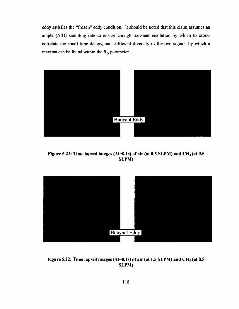
eddy satisfies the “frozen” eddy condition. It should be noted that this claim assumes an

ample (A/D) sampling rate to ensure enough transient resolution by which to cross

correlate the small time delays, and sufficient diversity o f the two signals by which a

maxima can be found within the Rxy parameter.

B uoyant Edd;

Figure 5.21: Time lapsed images (At=0.1s) of air (at 0.5 SLPM) and CH4 (at 0.5SLPM)

Figure 5.22: Time lapsed images (At=0.1s) of air (at 1.5 SLPM) and CH4 (at 0.5SLPM)

118

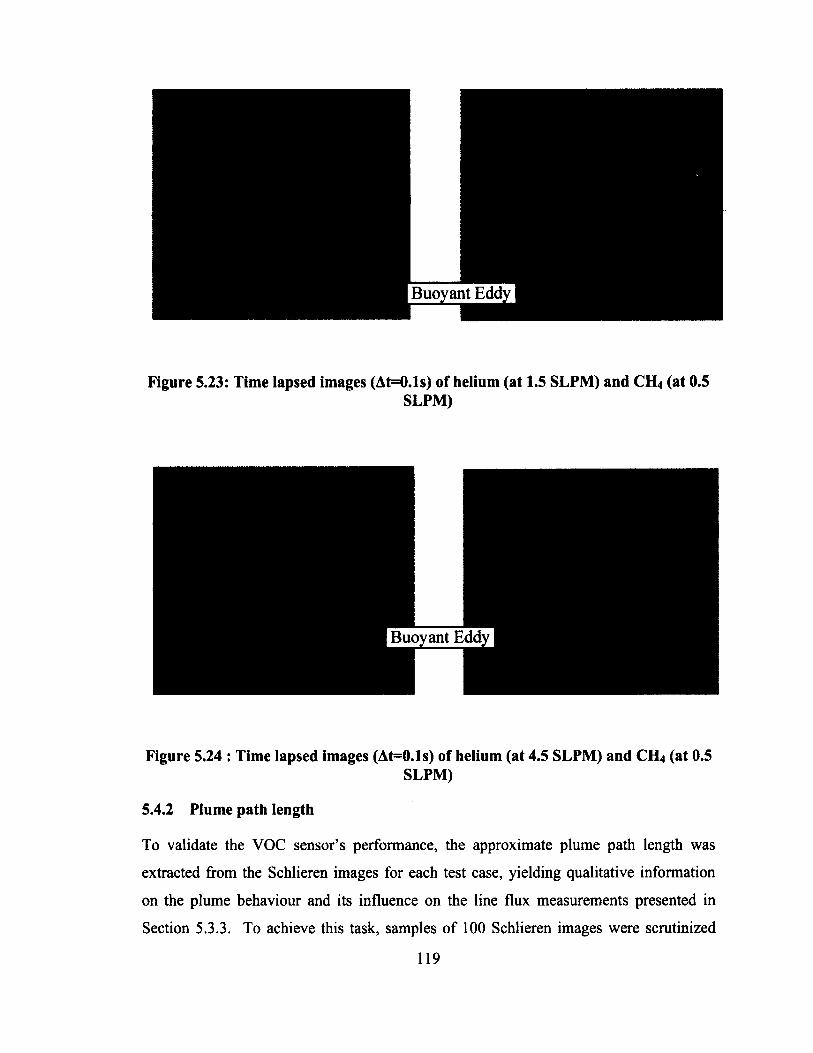
Buoyant Edd;

Figure 5.23: Time lapsed images (At=0.1s) of helium (at 1.5 SLPM) and CH4 (at 0.5SLPM)

Buoyant Edd;

Figure 5.24 : Time lapsed images (At=0.1s) of helium (at 4.5 SLPM) and CH4 (at 0.5SLPM)

5.4.2 Plume path length

To validate the VOC sensor’s performance, the approximate plume path length was

extracted from the Schlieren images for each test case, yielding qualitative information

on the plume behaviour and its influence on the line flux measurements presented in

Section 5.3.3. To achieve this task, samples of 100 Schlieren images were scrutinized

119

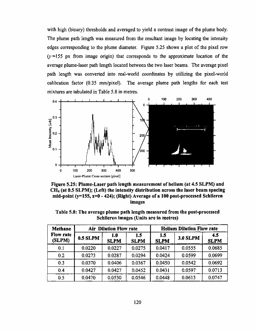
with high (binary) thresholds and averaged to yield a contrast image o f the plume body.

The plume path length was measured from the resultant image by locating the intensity

edges corresponding to the plume diameter. Figure 5.25 shows a plot of the pixel row

(y =155 px from image origin) that corresponds to the approximate location of the

average plume-laser path length located between the two laser beams. The average pixel

path length was converted into real-world coordinates by utilizing the pixel-world

calibration factor (0.35 mm/pixel). The average plume path lengths for each test

mixtures are tabulated in Table 5.8 in metres.

0.4

0.3 -

g 0.2 - 200/H

0.1 - '300 H

200 4000 100 300 500

Laser-Plume Cross section [pixel]

Figure 5.25: Plume-Laser path length measurement of helium (at 4.5 SLPM) and CH4 (at 0.5 SLPM); (Left) the intensity distribution across the laser beam spacing mid-point (y=155, x=0 - 424); (Right) Average of a 100 post-processed Schlieren

images

Table 5.8: The average plume path length measured from the post-processed Schlieren images (Units are in metres)



0.5 SLPM 1.0SLPM

1.5SLPM

1.5SLPM 3.0 SLPM 4.5

SLPM0.1 0.0220 0.0227 0.0275 0.0417 0.0555 0.0685

0.2 0.0273 0.0287 0.0294 0.0424 0.0599 0.0699

0.3 0.0370 0.0406 0.0367 0.0450 0.0542 0.06920.4 0.0427 0.0427 0.0452 0.0431 0.0597 0.07130.5 0.0470 0.0530 0.0546 0.0448 0.0613 0.0747

120

For the air-CH4 line flux measurements, the path length was found to increase by a

factor -2 , for an increase of methane from 0.1 SLPM to 0.5 SLPM, which in turn causes

the intercept of the fitted lines (as x—>0) to deviate from the expected y= ax trend.

However, the lower diffusivity o f air (in air) yielded minimal path length change as the

air flow rate increased from 0.5 SLPM to 1.5 SLPM, resulting in minimal change in the

overall slope between the line flux curves for the different air flow rates, as seen in

Figure 5.17. The helium-CH4 data, was found to behave in the opposite fashion, where

the path length increased slightly for an increase in the methane flow rate, but

significantly increased for increases in the helium flow rate (attributable to the high

diffusivity o f helium in air, -4 .5 times higher than that o f methane in air) and the higher

helium flow rates. This resulted in minimal deviation in the lower tail of the curve (from

the expected y=ax trend) but a more pronounced increase in the overall slope o f the curve

for the different helium-CH4 flux curves. Despite these complications, the proof of

concept dual-line CCV experiments demonstrate the potential utility o f this approach and

issues o f varying path-length through the plume should be readily resolved using a multi-

line, gridded laser beam system capable of resolving the full plume cross-section.

5.5 Cost-effective critique

To quantify the cost benefit of the VOC sensor, the total monetary investment was

scrutinized under the dollar per laser line criteria. The dollar per laser line is primary

controlled by the detector and its associated Mid-IR optical components, both on the laser

and detector side. This is due to the ample available power o f the HeNe laser source

which allows the creation of multiple laser lines per source. Taking this into

consideration along with the fact that the future VOC sensor’s acquisition electronics

would likely be implemented on the microcontroller level, the expected dollar per laser

line o f the novel VOC sensor is -$2300, yielding a monetary investment o f $73,600 for a

32 line VOC sensor. A complete breakdown of the experimental apparatus and its

associated costs are shown in Table 5.9.

121

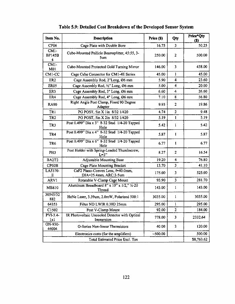
Table 5.9: Detailed Cost Breakdown of the Developed Sensor System

Item No. Description Price ($) Qty Prlce*Qty($)

CP06 Cage Plate with Double Bore 16.75 3 50.25CM1-

BP145B4

Cube-Mounted Pellicle Beamsplitter, 45:55, 3- 5um 250.00 2 500.00

CM1-M01 Cube-Mounted Protected Gold Turning Mirror 146.00 3 438.00

CM1-CC Cage Cube Connector for CM1-4E Series 45.00 1 45.00ER2 Cage Assembly Rod, 2”Long, 0 6 mm 5.90 4 23.60

ER05 Cage Assembly Rod, J4” Long, 0 6 mm 5.00 4 20.00ER3 Cage Assembly Rod, 3" Long, 0 6 mm 6.60 4 26.60ER4 Cage Assembly Rod, 4" Long, 0 6 mm 7.10 8 56.80

RA90 Right Angle Post Clamp, Fixed 90 Degree Adapter 9.93 2 19.86

TR1 PG POST, Sin X lin 8/32 1/420 4.74 2 9.48TR2 PG POST, Sin X 2in 8/32 1/420 5.19 1 5.19

TR3 Post 0.499” Dia x 3” 8-32 Stud 1/4-20 Tapped Hole 5.42 1 5.42

TR4 Post 0.499” Dia x 4” 8-32 Stud 1/4-20 Tapped Hole

5.87 1 5.87

TR6 Post 0.499” Dia x 6” 8-32 Stud 1/4-20 Tapped Hole

6.77 1 6.77

PH3Post Holder with Spring-Loaded Thumbscrew,

L=3” 8.27 2 16.54

BA2T2 Adjustable Mounting Base 19.20 4 76.80CP02B Cage Plate Mounting Bracket 13.70 3 41.10

LA5370-E

CaF2 Plano-Convex Lens, f=40.0mm, DIA=25.4mm, ARC:3-5um 175.00 3 525.00

ARV1 Rotatable V-Clamp Cage Mount 93.90 3 281.70

MB810 Aluminum Breadboard 8” x 10” x 1/2,” ‘A-20 Thread 143.00 1 143.00

30545/32882 HeNe Laser, 3.39um, 2.0m W, Polarized 500:1 3035.00 1 3035.00

64353 Filter ND LWIR 0.30D 25mm 295.00 1 295.00Cl 502 Post V-Clamp Mount 92.00 2 184.00

P VI-3.4- lx l

IR Photovoltaic Uncooled Detector with Optical Immersion 778.00 3 2332.64

ON-930-44004 O-Series Non-linear Thermistors 40.00 3 120.00

Electronics costs (for the amplifiers) -500.00 500.00Total Estimated Price Excl. Tax $8,763.62

122

Chapter 6

Conclusions and Future Work

6.1 Conclusions

This research project was the first investigation of DAS-CCV motivated by an

application to develop an economical VOC sensor that could measure hydrocarbon

emission rates from LSTs. The sensitivity and the uncertainty of the proposed DAS-CCV

technique were evaluated in proof-of-concept experiments to measure a line flux of a

hydrocarbon plume under lab conditions.

Sensor performance was evaluated in two main categories: transient response and

noise behavior. From 100 percent step input tests it was determined that

detector/amplifier had an average response time of 1.3 ms, inferring a cut-off frequency

of 770 Hz. Additionally, the step input tests showed very little overshoot (-0.03% ) in the

detector/amplifier response, resulting in very minimal transients (fluctuations) that could

cause erroneous cross correlations. The noise behaviour of the referenced signal showed

slight degradation from 1/f noise. However, the overall magnitude was found to be

below 0.1%, yielding good signal sensitivity.

The concentration sensitivity and uncertainty o f the VOC sensor was determined

in experiments to measure the volumetric fraction o f various methane-air mixtures in a

flow-through a spectroscopic cell. The steady state measurements demonstrated good

concentration sensitivities, with random error magnitudes (without averaging) o f 1.27%,

inferring a detection limit o f 2.22 ppm-m. The uncertainty o f the concentration

measurements determined using the ASTM TSM method, was found to be very good at

-1.35%.

123

The line flux sensitivity and uncertainty were determined by experimentally

measuring the path integrated concentration and the velocity o f the open flow

hydrocarbon plume. The velocity was measured using the DAS-CCV technique (to

extract the time delay corresponding to the maximum correlation between the measured

signals for the two beams). The air-methane data showed good linear agreement between

the measured eddy velocity and the methane mass flux o f the open flow plume. The

velocity measurement uncertainty for the air-methane data was found to lie between 2 to

7.5% for a sample set of 100. The path integrated concentration measurements of the air-

methane plumes also showed good linear agreement, with uncertainties ranging between

0.4 to 0.6%. Combining the measured eddy velocity and the path integrated

concentrations, the calculated air-methane line flux data showed good linear agreement

with the input mass flux with total uncertainties ranging between 2.5 to 6.9%.

The helium-methane data allowed tests at higher flow rates while still maintaining

sufficient density differences between the plume and the surrounding air for the Schlieren

imaging system. However, the measured helium-methane eddy velocities deviated from

the input methane mass flow to the plume, as the helium dilution flow increased. This is

due to the eddy behaviour being determined by both the methane and helium mass flow,

since both gases contribute to the buoyant nature of the plume. For the helium-methane

mixtures, the velocity uncertainty was found to lie between 5 to 16.5% for a sample set of

100. Path integrated concentration measurements o f the helium-methane plumes were

achieved with uncertainties ranging between 0.4 to 0.55%. From the measured eddy

velocity and the path integrated concentrations, the calculated helium-methane line flux

depicted good linear agreement with the input flow rate to the plume generator, with

higher uncertainties ranging between 2 to 19%. This was attributable to the relative

difference between the beam spacing and the characteristic eddy size of the plume, as

seen through the Schlieren imaging system, indicating that the beam spacing needed to be

reduced to satisfy the frozen eddy condition. Schlieren imaging confirmed this was not a

significant issue for the air-methane plumes

124

Setting aside these minor issues, from the traverse tests, the dual beam, proof-of-

concept system demonstrated that the DAS-CCV technique is a viable approach that

could potentially be utilized in a full scale, multi-beam, gridded sensor to measure the

emissions released by LSTs with good accuracy and for a relatively low monetary

investment.

6.2 Future Work

The four main issues that require further research to move the DAS-CCV sensor to the

field are the improvement of the detector-amplifier noise performance, control o f the

CCV beam spacing, more rigorous consideration o f the hydrocarbon speciation problem,

and the implementation of the multi-line grid DAS-CCV sensor.

6.2.1 Detector-Amplifler Noise Performance

From the noise performance tests, it was determined that the highest noise contributor

was either the PVI-3.4 detector or the 1st stage of the custom amplifier (or both). The 1/f

noise, commonly seen with use of semi-conductors, was found to be the highest noise

source in the system response. To reduce the 1/f noise at the detector, the amplifier

requires a redesign to allow the detector to be connected with a zero voltage bias (i.e.

connected to ground). According to the manufacturer, this will reduce the 1/f noise

produced by the detector. The amplifier requires a detailed analysis and if need be, a

redesign to remove any possible 1/f noise contributors (if any exist).

6.2.2 CCV Optimal Beam spacing

As stated previously, the reason for higher error in the velocity measurements of the

helium case study was the due to the fact that the beam spacing between the laser-beams

was too large, and could not satisfy the “frozen eddy” condition. The beam spacing

could thus be better optimized and it would be advisable to design a field system where

this might be easily varied using custom-made beam splitting optics.

125

6.2.3 Hydrocarbon speciation

To move the VOC sensor to field, the hydrocarbon speciation problem must be addressed

while maintaining the cost effective design requirements. The hydrocarbon speciation

problem lies in the fact that the emissions from LSTs are a multi-component mixture that

has high variation in composition, and while these hydrocarbon molecules all have good

absorption strengths in the mid-IR band, determining the individual concentration o f each

gas is impossible from DAS unless the composition was known a priori. Therefore, to

make the VOC sensor viable as a fully quantitative tool, further research and design for

the speciation problem must be conducted. Likely solutions include secondary extractive

gas sampling and analysis (e.g. via gas chromatography or combined gas chromatography

mass spectrometry) or secondary near-IR DAS. Extractive gas sampling could

potentially be conducted semi-continuously using a field deployable micro-gas

chromatograph to determine relative species concentrations and allow for quantitative

calibration o f the DAS signal. Alternatively, future research could consider the use of

one or two near-IR DAS (or WMS) laser lines within the mid-IR multi-line laser grid to

use the overtones of the fundamental absorption bands to differentiate between the multi-

component mixtures. A point of interest that will most likely limit (or prevent) the

application o f a secondary near-IR sensor is the location o f all the VOC absorption peaks

across the near-IR (wavelength) bandwidth and the strong interference o f H2 O

absorption. While the near-IR absorption peaks associated with hydrocarbon are sizably

more spread out over the light spectrum (for a singular species) than their mid-IR

counterparts, research conducted by Chung (2007) indicated that near-IR absorption of

crude oil and gasoline vapours proved difficult due to the overlapping o f absorption

features corresponding to all o f the hydrocarbon species that comprise crude oil and

gasoline. For example, gasoline has -150 individual species from C4 to C9

(hydrocarbons) which correspond to several hundred overlapping absorption features,

preventing selective measurement o f each species.

126

6.2.4 Multi-line CCV

To meet the ultimate goal o f developing a viable means for measuring emissions from

external floating roof tanks for which no practical alternatives exist, a critical next step in

the development o f the proof-of-concept apparatus will be to design and test a cost-

effective multi-beam system. Related research into tomographic data processing would

also be beneficial.

127

References

AIST, N. I. (2010). Spectral Database fo r Organic Compounds SDBS. Retrieved Febuary 20,2010, from http://riodb01.ibase.aist.go.jp/sdbs/cgi-bin/direct_frame_top.cgi

Amstrong, I., Johnstone, W., Duffin, K., Lengden, M., Chakraborty, A., & Ruxton, K. (2010, May 15). Detection o f CH4 in the Mid-IR Using Difference Frequency Generation With Tunable Diode Laser Spectroscopy. Journal o f Ligthwave Technology, 25(10).

Atcheson, B. (2007). Schlieren-Based Flow Imaging. M.A.Sc Thesis, University of British Columbia, Computer Science.

Bosch Jr., J., & Logan, T. (2006). VOC Fugitive Losses: New Monitors, Emision Losses, and Potential Policy Gaps. U.S. Environmental Protection Agency.

Chambers, A. K. (2004). Optical Measurement Technology fo r Fugitive Emissions from Upstream Oil and Gas Facilities. Carbon and Energy Management, Alberta Reseach Council Inc.

Chambers, A., Strosher, M., Wootton, T., Moncrieff, J., & McCready, P. (2006). DIAL Measurements o f Fugitive Emissions from Natural Gas Plants and the Comparison with Emission Factor Estimates. Alberta Research Council.

Cheng, L., Jeffries, J., & Hanson, R. (2010). Mass Flux Sensing via Tunable Diode Laser Absorption o f Water Vapor. AIAA Journal, 45(11).

Chu, T., & Hogg, D. (1966, Febuary). The Attenuation of 3.392 um He-NE LaserRAdiation by Methane in the Atmosphere. The Bell System Techincal Journal.

Cockbum, J. (2006). Mid-infrared Quantum Cascade Lasers. In Mid-infraredSemiconductor Optoelectronics (Vol. 118). Springer Series in Optical Sciences.

Coleman, H. (2009). Experimentaiton, validation and uncertainty analysis fo r engineers (3rd Edition ed.). Hoboken, New Jersey: John Wiley & Sons.

Cox, G., & Chitty, R. (1980). A Study o f the Deterministic Properties o f Unbounded Fire Plumes. Combustion and Flame, 39, 191-209.

Daun, K. (2010). Infrared species limited data tomography through Tikhonovreconstruction. Journal o f Qualitative Spectroscopy and Radiative Transfer, 111.

Dereniak, E., & Boreman, G. (1996). Infrared Detectors and Systems. New York: John Wiley & Sons Inc.

128

http://riodb01.ibase.aist.go.jp/sdbs/cgi-bin/direct_frame_top.cgi

Engineering Science, I. (1977). Hydrocarbon Emissions from Fixed-Roof Petroleum Tanks.

Env. Can., E. C. (2008). Canada’s Greenhouse Gas Emissions: Understanding the Trends. Retrieved September 29,2009, from http://www.ec.gc.ca/Publications/75805F15-908C-4FBl-A285- 6D437FF04C93/CanadasGreenhouseGasEmissionsUnderstandingTheTrendsl990 2006.pdf

EPA, E. P. (1995). AP 42: Compilation o f Air Pollutant Emission Factors, Volume I: Stationary Point and Area Sources.

Ferry, R. (2002). Emissions from Aboveground Storage Tanks. (TGB partneship) Retrieved Febuary 20, 2011, fromhttp://www.tgbpartnership.com/linked_data_files/tanks_3_0.pdf

Gieseler, H., Kessler, W., Finson, M., Davis, S., Mulhall, P., Bons, V., et al. (2007, July). Evaluation of Tunable Diode Laser Absorption Spectroscopy for In-Process Water Vapor Mass Flux Measurements During Freeze Drying. JOURNAL OF PHARMACEUTICAL SCIENCES, 96(1).

Grant, W. (1986, March 1). He-Ne and cw C 02 laser long-path systems for gas detection. Apllied Optics, 25(5).

Herrmann, K., Renneberg, A., & Kreuzer, H. (1987). Precision velocimetry with digital cross-correlation for flow measurements during thrombus growth. Microvascular research, 34( 1), 13-28.

Hindle, F., Carey, S., Winterbone, D., Clough, E., & McCann, H. (2001). Measurement of gaseous hydrocarbon distribution by a near-infrared absorption tomography system. Journal o f Electronic Imaging, 10(3).

HITRAN, H.-S. C. (2008). The HITRAN 2008 molecular spectroscopic database. Retrieved December 1,2009, from http://cfa-www.Harvard.edu/HITRAN

Hollas, J. (2004). Modern Spectroscopy. John Wiley & Sons, Inc.

IMPEL Network. (2000). Diffuse VOC Emisions. Brussels.

Klingbeil, A., Jeffries, J., & Hanson, R. (2006, June 12). Temperature- and pressure- dependent absorption cross sections o f gaseous hydrocarbons at 3.39 um. Measurement Science and Technology, 1950-1957.

Kllingbeil, A. (2007). MID-IR Laser Absortion Diagnostics fo r Hydrocarbon Sensing in Harsh Enviroments. Ph.D. Thesis, Stanford University, Department of Mechanical Engineering, Stanford.

129

http://www.ec.gc.ca/Publications/75805F15-908C-4FBl-A285-

http://www.tgbpartnership.com/linked_data_files/tanks_3_0.pdf

http://cfa-www.Harvard.edu/HITRAN

Kosterev, A., Wysocki, G., Bakhirin, Y., So, S., Lewicki, R., Fraser, M., et al. (2008).Application o f Quatum Cascade Lasers to Trace Gas Analysis. Applied Physics B, 90, 165-176.

Kuhnemann, F., Muller, F., G.V., B., Halmer, D., Popp, A., Schiller, S., et al. (2004).CW-OPO based cavity-leak-out spectrometer for ultra-sensitive and selective mid infrared trace gas analysis. Proceedings o f the SPIE, 5337, 117-127.

Lachish, U., Rotter, S., Adier, E,, & El-Hanany, U. (1987, June). Tunable diode laserbased spectroscopic system for ammonia detection in human respiration. Review o f Scientific Instuments, 58(6).

Land and Marine Project Engineering Ltd. (n.d.). Internal Floating R oo f Retrieved Febuary 20,2011, fromhttp://www.landandmarine.com/TankServProducts/IntemalFloatingRoof.aspx

Long, B., & Gamer, B. (2004). Guide to Storage Tanks and Equipment. John Wiley and Sons.

Lubken, F., Dingier, F., Lucke, H., Anders, J., Riedel, W., & Wolf, H. (1999, September 1). MASERATI: a rocketbome tunable diode laserabsorption spectrometer. Apllied Optics, 55(25).

Lyle, K. (2005). Developement o f a Real-Time Diode -Laser Mass flux Sensor fo r simultaneous Measurement o f Density and Velocity o f Oxygen. TSD Report, Stanford University, High Temperature Gasdynamics Laboratory, Mechanical Engineering Department, Stanford.

Mell, W., McGrattan, K., & Baum, H., (1996). Numerical simulation o f combustion in fire plumes. 26th Symposium on Combustion/The combustion Institute.

Mellqvist, J., Samuelsson, J., Galle, B., & Kihlman, M. (2006). The Solar Occultation Flux Method, a new techniue to quantify fugitive VOC emissions. CEM2006. 7th International Conference on Emission Monitoring”. Paros.

Mellqvist, J., Samuelsson, J., Offerle, B., Salberg, H., Johansson, J., & Jaakkola, S.(2009). Emission Measurements o f Volatile Organic Compounds with the SOF method in the Rotterdam Harbor 2008. Goterborg: FluxSense.

Mielenz, K., & Nefflen, K. (1965). Gas Mixtures and Pressures for Optimum Output Power o f Rf-Excited Helium—Neon Gas Lasers at 632.8 nm. Applied Optics, 4(5).

Mohamed, A., & Lefebvre, M. (2009). Laser Absorption Spectroscopy to probe chemically reacting flows. The onera journal Aerospace Lab( 1).

130

http://www.landandmarine.com/TankServProducts/IntemalFloatingRoof.aspx

Morgan, M., & Bowles, K. (1968, September 13). Cross-Correlation and Cross-Spectral Methods for Drift Velocity Measurements. Science, New Series, 76/(3846), 1139- 1142.

Myers, P. (1997). Aboveground Storage Tanks. New York: M cGraw-Hill.

Pal, S., Ozanyan, K., & McCAnn. (2008). A computational study o f tomographicmeasurement o f carbon monoxide at minor concentrations. Measurement Science and Technology, 19(9).

Pashotta, R. (2008). Encyclopedia o f Laser Physic and Technology, Vols.b I & I I ”. Weinheim: Wiley-VCH Verlag GmBH & Co.

Pasley, H., & Clark, C. (2000). Computational fluid dynamics study of flow around a floating-roof oil storage tanks. Journal o f Wind Engineering and Industrial Aerodynamics,, 86.

Philippe, L., & Hanson, R. (1991, December 15). Laser-absorption mass flux sensor for high-speed airflows. Optics Letters, 76(24).

Picard, D. (2009). Estimating Average and Instantaneous Emmssions Rates from Hydrocarbon Liquid Storage Taniks. Clearstone Engineering Ltd.

Piotrowski, J., & Rogalsk, A. (2007). High Operating Temperature Infrared Photodetectors. Washington: SPIE.

Pouchert, C. (1981). The Aldrich libraryof infrared spectra. Milwaukee: Aldrich Chemical Co.

Rieker, G. (2009). Wavelength-Modulation Spectroscopy fo r Measurements o f Gas Temperature and Concentraiton in Harsh Enviroments. PhD Thesis, Stanford University, Mechanical Engineering.

Rockwell, S., Rangwala, A., & Klein, A. (2009). An investigation into the use o f Cross Correlation Velocimetry. MSc Thesis, Worcester Polytechnic Institute.

Settles, G.S. (2001). Schlieren and shadowgraph techniques: visualizing phenomena in transparent media. New York: Springer-Verlag.

Shorter, J. H., Nelson, D. D., Milton, D. K., Sama, S., & Zahniser, M. S. (2010). Clinical Study O f Multiple Biomarkers In The Breath O f Asthma And COPD Patients Using A Fully Automated Quantum Cascade Laser Spectrometer. American Journal o f Respiratory andCritical Care Medicine.

Skeldon, K., McMillan, L., Wyse, C., Monk, S., Gibson, G., Patterson, C., et al. (2006). Application o f laser spectroscopy for measurement of exhaled ethane in patients with lung cancer. Respiratory Medicine, 100,300-306.

131

So, S., Sani, A., Zhong, L., Tittel, F., & Wysocki, G. (2009, April 16). Laser Spectroscopic Trace-Gas Sensor Networks for Atmospheric Monitoring Applications. Workshop on Sensor Networks fo r Earth and Space Science Applications (ESSA).

Spectrasyne Ltd. (2010). Spectrasyne, Enviromental Surveying. Retrieved October 20, 2010

Springholz, G., Schwarzl, T., & Heiss, W. (2006). Mid-infrared Vertical Cavity Surface Emitting Lasers based on the Lead Salt Compounds. In Mid-infrared Semiconductor Optoelectronics (Vol. 118). Springer Series in Optical Sciences.

Svensson, T., Andersson, M., Rippe, L., Svanberg, S., Andersson-Engels, S., Johansson, J., et al. (2008). VCSEL-based oxygen spectroscopy for structural analysis of pharmaceutical solids. Applied Physics B: Laser and Optics , 345-3554.

Thorlabs Ltd. (2011). Retrieved Febuary 10, 2011, from Available: http://www.thorlabs.com/

Tittel, F. K., Richter, D., & Fried, A. (2003). Mid-Infrared Laser Applications inSpectroscopy. In I. T. Sorokina, & K. L. Vodopyanov (Eds.), Solid-State Mid- Infrared Laser Sources (Vol. 89, pp. 445-510). Springer-Verlag.

Tittel, F., Lancaster, D., Richter, D., Golberg, L., & Koplow, D. (1999). Compact Mid- Infrared Trace Gas Sensor Based on Difference Frequency Mixing. SPIE, 3758.

Topfer, T., Petrov, K., Mine, Y., Jundt, D., Curl, R., & Tittel, F. (1997, October 20). Room-temperature mid-infrared laser sensor for trace gas detection. Applied Optics, 36(30).

Weber, M. (1999). Handbook o f Laser Wavelengths. CRC Press LLC.

Wofsy, S. (2011). HIAPER Pole-to-Pole Observations (HIPPO) fine-grained, global- scale measurements o f climatically important atmospheric gases and aerosols. Philosophical Transactions o f The Royal Soceity A: Mathematical Physical & Engineering Sciences, 369, 2073-2086.

Wright., P., Garcia-Stewart, C., Carey, S., Hindle, F., Pegrum, S., Colbume, S., et al.(2005, November 1). Toward in-cylinder absorption tomography in a production engine. Applied Optics, 44(31).

132

http://www.thorlabs.com/

Appendix A

Mechanisms of Evaporative Losses from

Liquid Storage TanksEvaporative losses from liquid storage tanks can be generalized into three main

categories: standing losses, working loses, and flashing losses. The relative contributions

of the various modes o f emissions differ with tank design.

A .l W orking Losses o f Liquid Storage Tanks

Working losses occur during the emptying-filling cycles as the liquid level changes. For

fixed roof tanks and horizontal tanks, working losses are comprised o f the hydrocarbon

saturated air that is displaced when the liquid level rises (i.e. during the filling

cycle)(Myers, 1997; EPA, 1995). For EFRTs, working losses mostly are due to

“clingage losses”, which occur during the withdrawal phase (i.e. the emptying cycle)

when the residual organic liquid on the side walls is exposed to the atmosphere allowing

for convective evaporation. While clingage does occur in IFRTs, the fixed roof (above

the internal floating roof) shields the crude oil clingage from convective mass transfer

(due to cross wind flows) only allowing diffusion/evaporative mass transfer. However,

EPA (1995) does not distinguish between the two modes o f mass transfer and simply

states that it is proportional to the exposed surface area and annual throughput (flow rate)

(Myers, 1997).

A.2 Standing Losses o f Liquid Storage Tanks

Standing storage losses are directly dependent on the storage tank design due to the fact

that they encompass all the operational losses from all the operational fittings and seals of

LSTs. Standing emission losses are defined as the evaporative losses that occur

independent o f liquid-level change in the tank (EPA, 1995). They are the losses that are

133

driven by changes in temperature and pressure. For EFRTs, standing losses also include

any evaporative losses driven by crosswind flow (Myers, 1997; EPA, 1995). These

driving forces result in a differential pressure across the various fittings which promote

losses through either the pressure valves or through seal permeation (Myers, 1997).

A.2.1 Standing Losses o f Floating R oof Storage Tanks

The standing losses from floating roof tanks are further sub-divided into standing losses

associated with the floating ro o fs perimeter seal (known as deck rim seal loses) and the

standing losses associated with all the combined losses from operational fittings that

penetrate the floating roof (known as deck fitting losses).

Deck rim seal losses

Deck rim seal losses occur due to many complex mechanisms that vary with the different

deck rim seal designs. However, it has been documented for EFRTs that the bulk of the

deck rim seal losses are wind-induced (Myers, 1997). While the fixed outer roof o f the

IFRT minimizes the effect o f cross-wind flow, crosswinds can still promote evacuation of

the emissions from the head space of the IFRT (between the fixed roof and internal

floating roof). Other non-dominant mechanisms that have been noted to promote losses

through the deck rim seals are variations in the operating temperature and pressure.

Various designs o f the EFRT deck rim seals can be seen in Figure A .l (Myers, 1997;

EPA, 1995)

134

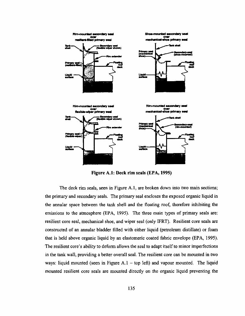
Rim-motntod Moondary Mai ovw

rmManfrfited primary Mai

Shoa-mountad aaoondary Mai ovar

maohanicat-«ho« primary Mai -IM ia h a l

PrfmawMM(nOHMHM)

Rlnwrtoontod saoondary aaal ovar

AaxfbJa-wripar primary MaiTM

Rlnvmountad aacortdary aaal ovar

machanlcal-ahoa primary aaal

ta o m y o a(rinHiwunM)

Figure A.l: Deck rim seals (EPA, 1995)

The deck rim seals, seen in Figure A. 1, are broken down into two main sections;

the primary and secondary seals. The primary seal encloses the exposed organic liquid in

the annular space between the tank shell and the floating roof, therefore inhibiting the

emissions to the atmosphere (EPA, 1995). The three main types o f primary seals are:

resilient core seal, mechanical shoe, and wiper seal (only IFRT). Resilient core seals are

constructed o f an annular bladder filled with either liquid (petroleum distillate) or foam

that is held above organic liquid by an elastomeric coated fabric envelope (EPA, 1995).

The resilient core’s ability to deform allows the seal to adapt itself to minor imperfections

in the tank wall, providing a better overall seal. The resilient core can be mounted in two

ways: liquid mounted (seen in Figure A .l - top left) and vapour mounted. The liquid

mounted resilient core seals are mounted directly on the organic liquid preventing the

135

formation of a rim vapour space (volume of air exposed to the organic liquid). The

vapour mounted resilient seal which does allow a rim vapour space is documented by

EPA (1995) to allow the highest rim losses (for EFRT), roughly 9-40 times that of the

liquid mounted rim for a wind speed of 5-15mph respectively. The mechanical shoe seal

is comprised o f a metal plate held in compression against the tank wall with a flexible

fabric cover to enclose the rim vapour space. EPA (1995) reports that this seal allows

roughly double the fugitive emissions when compared to the liquid mounted resilient seal

for ERFTs. Primary wiper seals (only IFRT) allow emission loses on par with vapour-

mounted resilient seals (EPA, 1995).

The secondary seals are a continuous seal mounted on the upper-most part of the

rim and act as a barrier against emissions that would come from the small openings or

tears in primary seal. The secondary seals are generally manufactured from flexible

polymeric materials. While this allows the seal to be held in compression against the

tank wall providing a robust barrier, they deteriorate due to debris and exposure to the

elements (Myers, 1997). To prolong the life of the secondary seals, weather shields can

be incorporated to provide added protection. The weather shields are constructed o f thin

overlapping steel sheets that are pivoted to ride the tank wall at an inclined angle (EPA

1995).

Myers (1997) states that the deck rim seals used for IFRT generally incorporate

either a resilient foam-filled seal or wiper seal, similar to those of EFRT, as the primary

seal. Since IFRTs are not significantly affected by the surrounding conditions (more

specifically crosswind flow), the deck rim seal is mainly designed to compensate for

small irregularities in the tank wall (EPA, 1995). The secondary seal is achieved through

the implementation o f a foam or wiper seal above the primary seal. While secondary

seals for IFRTs may be used to provide added protection against emission losses, they are

not commonly used unless specifically stated by the EPA’s pollution control standards

determined by the organic liquid being stored (EPA, 1995).

136

Deck fitting losses

Other documented sources o f evaporative losses are the various deck fittings that

penetrate the floating roof allowing for vapour exchange between the organic liquid and

the surroundings. The most common fittings that contribute to evaporative losses are:

The design of each type of deck fitting can be seen in Figure A .l, Figure A.3 and

Figure A.4. The access hatch is an opening in the floating roof deck with a peripheral

well that penetrates the floating roof. They are typical sized to allow access to workers or

required materials during construction and maintenance o f the floating roof tank. These

openings are closed using a removable cover that can either be left resting on the opening

or bolted and/or gasketed to reduce evaporative losses from the vapour head space,

located in the well (Myers, 1997; EPA, 1995)

A gauge float is used to determine the liquid level in the storage tank. It is a

buoyant float that lies on the liquid surface and is connected to an indicator on the

exterior o f the tank via a cable and guide system. The gauge float well (where the gauge

is housed) employs a sliding cover that moves with the floating roof and employs a

bushing to allow dynamic penetration of the cable through the sliding cover. Emissions

from the gauge float well can be reduced by bolting and/or gasketing the cover to the well

wall (Myers, 1997; EPA, 1995).

Gauge hatch/sample ports consist o f a pipe sleeve that penetrates the floating roof

allowing access to the organic liquid being stored within the tank. The top of the pipe

sleeve exposed to the surrounding is enclosed using a self-closing gasketed cover. The

gauge sample ports are sized to allow hand sampling or sampling from the gauger’s

platform (Myers, 1997; EPA, 1995).

The evaporative losses that occur from these fittings are determined by the ability

(or more specifically the inability) o f the sealing technology implemented to prevent

• Access hatches • Deck drains

• Gauge float wells

• Gauge hatch/Sample ports

• Rim vents

• Slotted unslotted guide poles

• Ladder Wells

• Vacuum Breaker

137

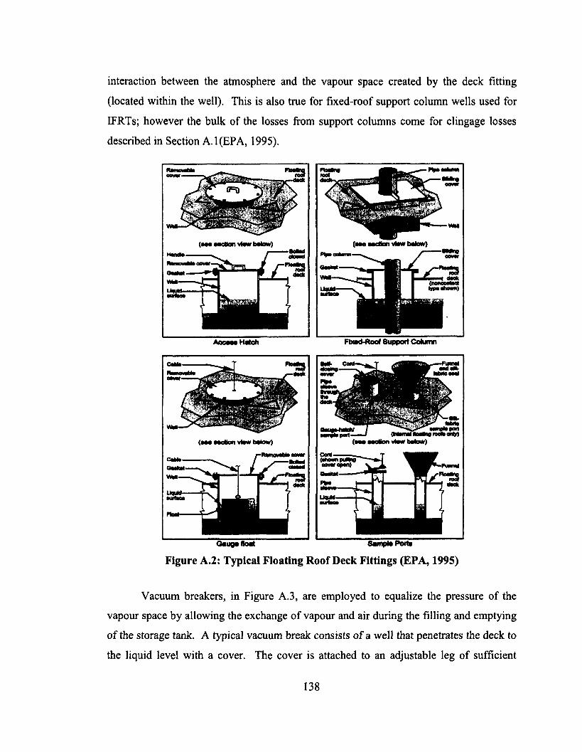
interaction between the atmosphere and the vapour space created by the deck fitting

(located within the well). This is also true for fixed-roof support column wells used for

IFRTs; however the bulk o f the losses from support columns come for clingage losses

described in Section A .l (EPA, 1995).

{ ••a Mc&on vt*w batow)

Aocaas Hatch Fbwd-Roof 8upport Column

Gauga float Sampta Porta

Figure A.2: Typical Floating Roof Deck Fittings (EPA, 1995)

Vacuum breakers, in Figure A.3, are employed to equalize the pressure of the

vapour space by allowing the exchange o f vapour and air during the filling and emptying

o f the storage tank. A typical vacuum break consists o f a well that penetrates the deck to

the liquid level with a cover. The cover is attached to an adjustable leg of sufficient

138

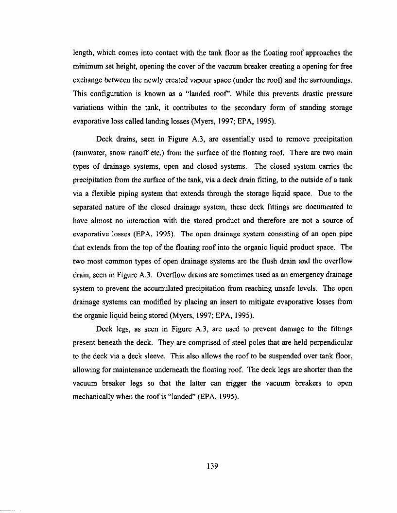
length, which comes into contact with the tank floor as the floating roof approaches the

minimum set height, opening the cover of the vacuum breaker creating a opening for free

exchange between the newly created vapour space (under the roof) and the surroundings.

This configuration is known as a “landed ro o f’. While this prevents drastic pressure

variations within the tank, it contributes to the secondary form o f standing storage

evaporative loss called landing losses (Myers, 1997; EPA, 1995).

Deck drains, seen in Figure A.3, are essentially used to remove precipitation

(rainwater, snow runoff etc.) from the surface of the floating roof. There are two main

types o f drainage systems, open and closed systems. The closed system carries the

precipitation from the surface o f the tank, via a deck drain fitting, to the outside o f a tank

via a flexible piping system that extends through the storage liquid space. Due to the

separated nature o f the closed drainage system, these deck fittings are documented to

have almost no interaction with the stored product and therefore are not a source of

evaporative losses (EPA, 1995). The open drainage system consisting of an open pipe

that extends from the top of the floating roof into the organic liquid product space. The

two most common types of open drainage systems are the flush drain and the overflow

drain, seen in Figure A.3. Overflow drains are sometimes used as an emergency drainage

system to prevent the accumulated precipitation from reaching unsafe levels. The open

drainage systems can modified by placing an insert to mitigate evaporative losses from

the organic liquid being stored (Myers, 1997; EPA, 1995).

Deck legs, as seen in Figure A.3, are used to prevent damage to the fittings

present beneath the deck. They are comprised o f steel poles that are held perpendicular

to the deck via a deck sleeve. This also allows the roof to be suspended over tank floor,

allowing for maintenance underneath the floating roof. The deck legs are shorter than the

vacuum breaker legs so that the latter can trigger the vacuum breakers to open

mechanically when the roof is “landed” (EPA, 1995).

139

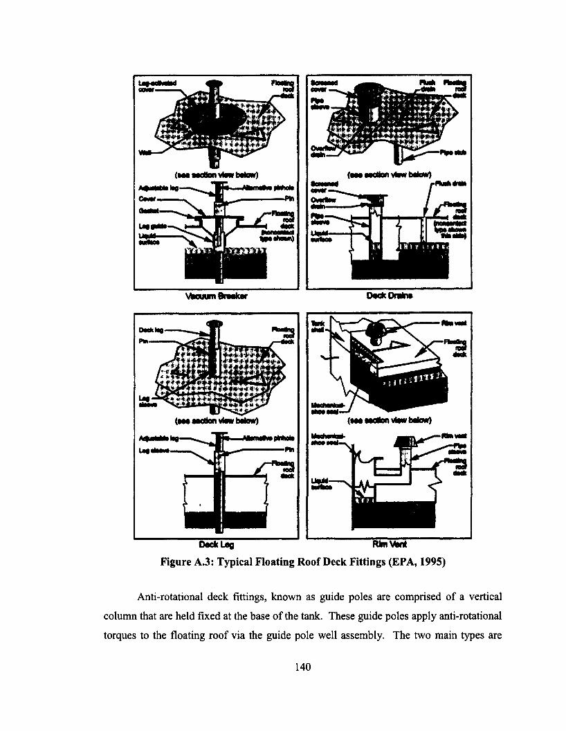
VKUum Breaker Deck Drain*

(•MMCtlonvtowbaHw)(199 9 9 0 0 1 VVW D99WJ

Deck Lag Rim Vent

Figure A.3: Typical Floating Roof Deck Fittings (EPA, 1995)

Anti-rotational deck fittings, known as guide poles are comprised of a vertical

column that are held fixed at the base o f the tank. These guide poles apply anti-rotational

torques to the floating roof via the guide pole well assembly. The two main types are

140

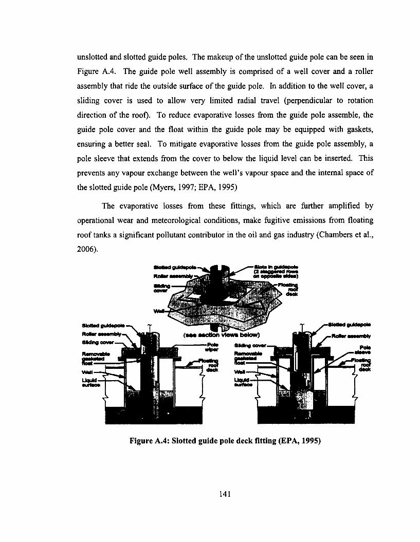
unslotted and slotted guide poles. The makeup of the unslotted guide pole can be seen in

Figure A.4. The guide pole well assembly is comprised o f a well cover and a roller

assembly that ride the outside surface o f the guide pole. In addition to the well cover, a

sliding cover is used to allow very limited radial travel (perpendicular to rotation

direction of the roof). To reduce evaporative losses from the guide pole assemble, the

guide pole cover and the float within the guide pole may be equipped with gaskets,

ensuring a better seal. To mitigate evaporative losses from the guide pole assembly, a

pole sleeve that extends from the cover to below the liquid level can be inserted. This

prevents any vapour exchange between the well’s vapour space and the internal space of

the slotted guide pole (Myers, 1997; EPA, 1995)

The evaporative losses from these fittings, which are further amplified by

operational wear and meteorological conditions, make fugitive emissions from floating

roof tanks a significant pollutant contributor in the oil and gas industry (Chambers et al.,

2006).

( m m M o t io n views below)--------- -Pota Mdbie«M

Figure A.4: Slotted guide pole deck fitting (EPA, 1995)

141

Standing Losses fo r Landed Floating Roofs

As stated earlier landing losses occur after the floating roof reaches its minimum height

and the vacuum breakers are mechanically engaged to equalize the pressure under the

floating roof as the liquid continues to drop, leading to landing losses. These losses are

amplified in EFRTs by crosswind flow which continually drives evaporative losses (EPA,

1995). The three main categories o f a landed roof can be seen in Figure A.5. The

breathing losses from a landed roof will remain dominant so long as there exists, wetted

areas across the floor o f the tank. Furthermore, during the initial filling o f the tank (when

the roof is landed), the addition of more liquid stock will displace the “heavier” (non-

buoyant) hydrocarbon vapours present under the deck further promoting evaporative

losses (Myers, 1997; EPA, 1995).

Full Liquid Heel Partial -Liquid Heel Drain Pry(standing liquid (standing liquid only (no standing liquid,

across the entire bottom) in or near a sump; only liquid is clingage)clingage elsewhere)

Figure A.5: Different configurations of a “landed” internal roof (EPA, 1995)

A.2.2 Standing Losses o f Fixed R oof Tanks and Horizontal Tanks

The standing losses for fixed roof and horizontal tanks are limited to sample ports, roof

access holes, and breather vents. Myers (1997) indicates that generally most breather

vents are/or have been modified to include pressure/vacuum valves, but if the breather

vent is simply left open to atmosphere, all other standing losses are negligible in

comparison. The sample port and access hole fittings for fixed roof tanks and

142

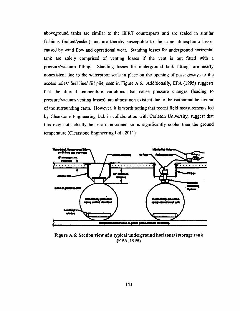
aboveground tanks are similar to the EFRT counterparts and are sealed in similar

fashions (bolted/gasket) and are thereby susceptible to the same atmospheric losses

caused by wind flow and operational wear. Standing losses for underground horizontal

tank are solely comprised of venting losses if the vent is not fitted with a

pressure/vacuum fitting. Standing losses for underground tank fittings are nearly

nonexistent due to the waterproof seals in place on the opening of passageways to the

access holes/ fuel line/ fill pile, seen in Figure A.6. Additionally, EPA (1995) suggests

that the diurnal temperature variations that cause pressure changes (leading to

pressure/vacuum venting losses), are almost non-existent due to the isothermal behaviour

of the surrounding earth. However, it is worth noting that recent field measurements led

by Clearstone Engineering Ltd. in collaboration with Carleton University, suggest that

this may not actually be true if entrained air is significantly cooler than the ground

temperature (Clearstone Engineering Ltd., 2011).

MiMi

i«MM ■M

Figure A.6: Section view of a typical underground horizontal storage tank(EPA, 1995)

143

Appendix B

Current Models for Estimating Emissions

from Liquid Storage TanksCurrent models for estimating evaporative losses from liquid storage tanks are based on a

series of semi-empirical algorithms developed through work cooperatively sponsored by

the American Petroleum Institute (API) and the U.S. Environmental Protection Agency

(EPA), and are detailed in Chapter 7.1 of AP-42 (EPA, 1995). Through the effort of

EPA’s office o f air quality and standards in technology transfer networking, the

algorithms have been published as a freeware emission-calculating program known as

TANKS (current version is 4.09) (EPA, 1995).

EPA TANKS is a Windows based computer program that allows for the user to

estimate the annual average emissions when the tank characteristics, turnover per year,

average vapour pressure, and average ambient temperature are specified. The flashing

losses described in Chapter 1 are not taken into account in AP-42 emission estimates.

This is because the estimates were designed to represent the storage o f stable liquids (i.e.

all liquid) and therefore does not account for trapped hydrocarbon gasses within the

organic liquid that “flash” out during the filling cycle (EPA, 1995).

B .l Emission Factors o f Floating R oof Tanks

The current emission estimating algorithms for floating roof tanks are presented here in

three parts: standing losses, working losses and landed roof losses. For floating roof

tanks, the working losses are solely comprised o f the clingage losses (for EFRT) or filling

losses (for IFRT) due to change o f the liquid level of the tank. For an EFRT, as the liquid

level is reduced, the floating roof descends and exposes the tank’s inner “wetted” surface

to the atmosphere, allowing for (“clingage”) evaporative losses. For an IFRT, a change in

144

the level of the internal floating roof induces an exchange of gases between the vapour

space above the floating roof (within the tank) and the surroundings, since the fixed

external roof does not sustain a pressure difference and must exchange gas with the

ambient environment to regulate the internal pressure. During the filling cycle o f an

IFRT, any hydrocarbon vapours above the internal floating roof are displaced through

vents in the fixed outer roof into the atmosphere.

The standing losses (also known as breathing losses) are broken down into two

main groups, the losses from the deck rim seal and those of the multiple deck fittings that

penetrate the deck. The fugitive emission estimates from standing losses do not take into

to account long term transients such as wear and destruction o f gasket seals or fittings,

which would contribute to higher wind induced emissions (EPA, 1995).

The total annual evaporative losses are estimated by the relation presented in

Equation B .l. The evaporative losses that are generated when the floating roof is landed

are separately considered, since those losses are estimated on a per episode basis and

differ depending on the landed roof scenarios (EPA, 1995).

Lt = Lr + Lwd + Lp + Lp (B .l)

where:

Lt is the total evaporative losses [Ib/yr],

Lr is the rim seal evaporative losses [lb/yr],

LF is the deck fitting evaporative losses [lb/yr],

Lwd is the evaporative loss due to withdrawal [lb/yr], and

LD is the deck seam losses (IFRT’s only) [lb/yr]

B.1.1 Standing loses o f Floating R oof Tanks

Rim seal losses can be estimated via Equation B.2 (EPA, 1995):

LR = GKRa + KRb • v n)D ' P* • M v • Kc (B.2)

where:

KRa is the zero wind speed rim seal loss factor [lb-mole/ft-yr],

145

KRb is the wind dependent rim seal loss factor [lb-mole/(mph)n-ft-yr],

v is the average ambient wind speed at tank site (is zero for IFRT) [mph],

n is the seal related wind speed exponent fitting evaporative loss [-],

D is the storage tank diameter [ft],

Mv is the average molecular weight o f the liquid stock [lb/lb-mole],

Kc is the product factor [-] (0.4 for crude oils; 1 for all other organic liquids), and

P* is the vapour pressure function [-] (see Equation B.3 for further details).

The wind dependent behaviour of Equation B.2 was determined through

experimental testing at equilibrium conditions and at fixed wind speeds (from 2.2 to

13.1 mph) (EPA, 1995). In these tests, hydrocarbon measurements were conducted

downstream at steady state conditions to determine the release rates for each test

condition and based on these data, the annual emission rate was determined assuming an

annual average wind speed. However, since the wind speed is exponentially related to

the standing losses, the error in the estimate also grows in a similar fashion, as

determined by a sensitivity analysis conducted by EPA (1995).

From the same sensitivity analysis it was determined that the error introduced by

using an average wind speed rather than averaging the standing loses over the annual

period that uses the annual wind speed distribution, is dependent on the dimensionless

wind speed exponent (as seen in Equation B.2) and the coefficient o f variation (i.e. the

ratio between standard deviation to the mean) of the wind speed (EPA, 1995). It was

found that for a coefficient of variation of 0.45 to 0.6, the error induced for wind speed

exponents o f 0.4 and 1.5 were between 2 to 5% and 7 to 11% respectively. However for

a wind speed exponent of 2.6, the error induced for the same coefficient o f variation

range, was found to be 30 to 45% (EPA, 1995). For wind speed exponents greater than

the 1.5, EPA (1995) recommended that a detailed wind speed distribution be taken into

account. See Table B .l, for additional details on KRa and KRb factors (EPA, 1995).

146

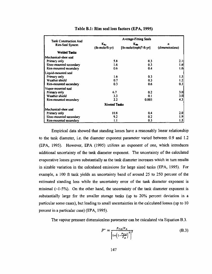
Table B.l: Rim seal loss factors (EPA, 1995)

Tank Construction AndAverage-Fitting Seals

Rim-Scal System Km K m, n(Ib-mole/ft-yr) [lb-molc/(mph) -ft-yr] (dimensionless)

Welded TanksMechanical-shoe seal

Primary only 5.8 0.3 2.1Shoe-mounted secondary 1.6 0.3 1.6Rim-mounted secondary 0.6 0.4 1.0

Liquid-mounted sealPrimary only 1.6 0.3 1.5Weather shield 0.7 0.3 1.2Rim-mounted secondary 0.3 0.6 0.3

Vapor-mounted sealPrimary only 6.7 0.2 3.0Weather shield 3.3 0.1 3.0Rim-mounted secondary 2.2

Riveted Tanks0.003 4.3

Mechanical-shoe sealPrimary only 10.8 0.4 2.0Shoe-mounted secondary 9.2 0.2 1.9Rim-mounted secondary l.l 0.3 1.5

Empirical data showed that standing losses have a reasonably linear relationship

to the tank diameter, i.e. the diameter exponent parameter varied between 0.9 and 1.2

(EPA, 1995). However, EPA (1995) utilizes an exponent of one, which introduces

additional uncertainty o f the tank diameter exponent. The uncertainty o f the calculated

evaporative losses grows substantially as the tank diameter increases which in turn results

in sizable variation in the calculated emissions for large sized tanks (EPA, 1995). For

example, a 100 ft tank yields an uncertainty band o f around 25 to 250 percent of the

estimated standing loss while the uncertainty error o f the tank diameter exponent is

minimal (~l-5%). On the other hand, the uncertainty o f the tank diameter exponent is

substantially large for the smaller storage tanks (up to 20% percent deviation in a

particular some cases), but leading to small uncertainties in the calculated losses (up to 10

percent in a particular case) (EPA, 1995).

The vapour pressure dimensionless parameter can be calculated via Equation B.3.

p v a / p a

147

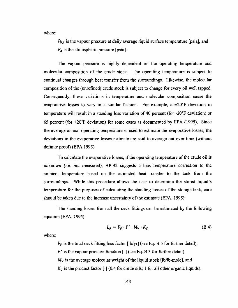
where:

PVA is the vapour pressure at daily average liquid surface temperature [psia], and

PA is the atmospheric pressure [psia].

The vapour pressure is highly dependent on the operating temperature and

molecular composition of the crude stock. The operating temperature is subject to

continual changes through heat transfer from the surroundings. Likewise, the molecular

composition o f the (unrefined) crude stock is subject to change for every oil well tapped.

Consequently, these variations in temperature and molecular composition cause the

evaporative losses to vary in a similar fashion. For example, a ±20°F deviation in

temperature will result in a standing loss variation of 40 percent (for -20oF deviation) or

65 percent (for +20°F deviation) for some cases as documented by EPA (1995). Since

the average annual operating temperature is used to estimate the evaporative losses, the

deviations in the evaporative losses estimate are said to average out over time (without

definite proof) (EPA 1995).

To calculate the evaporative losses, if the operating temperature o f the crude oil is

unknown (i.e. not measured), AP-42 suggests a bias temperature correction to the

ambient temperature based on the estimated heat transfer to the tank from the

surroundings. While this procedure allows the user to determine the stored liquid’s

temperature for the purposes o f calculating the standing losses o f the storage tank, care

should be taken due to the increase uncertainty o f the estimate (EPA, 1995).

The standing losses from all the deck fittings can be estimated by the following

equation (EPA, 1995).

Lf = Fp • P * ' Mv • Kc (B.4)

where:

Fp is the total deck fitting loss factor [lb/yr] (see Eq. B.5 for further detail),

P* is the vapour pressure function [-] (see Eq. B.3 for further detail),

Mv is the average molecular weight o f the liquid stock [lb/lb-mole], and

Kc is the product factor [-] (0.4 for crude oils; 1 for all other organic liquids).

148

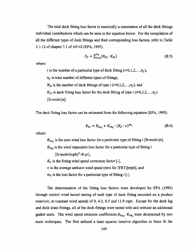
The total deck fitting loss factor is essentially a summation of all the deck fittings

individual contributions which can be seen in the equation below. For the compilation of

all the different types o f deck fittings and their corresponding loss factors, refer to Table

3.1-12 of chapter 7.1 of AP-42 (EPA, 1995).

Ff = (B.5)where:

i is the number of a particular type of deck fitting (H ) ,l ,2 ,. . .,n} ),

rif is total number of different types o f fittings,

NFi is the number of deck fittings of type i (i=0,l,2,. and

Kfi is deck fitting loss factor for the deck fitting of type i (/=0,1 ,2 , . . .,rif)

[lb-mole/yr].

The deck fitting loss factor can be estimated from the following equation (EPA, 1995).

KFi = KFat + KFbi • (Ky • v )m< (B.6)

where:

Kpai is the zero wind loss factor for a particular type of fitting i [lb-mole/yr],

KFbl is the wind dependent loss factor for a particular type o f fitting i

[lb-mole/(mph)m-ft-yr],

Kv is the fitting wind speed correction factor [-],

v is the average ambient wind speed (zero for IFRT)[mph], and

m f is the loss factor for a particular type of fitting i [-].

The determination of the fitting loss factors were developed by EPA (1995)

through control wind tunnel testing of each type of deck fitting mounted on a product

reservoir, at constant wind speeds o f 0, 4.3, 8.5 and 11.9 mph. Except for the deck leg

and deck drain fittings, all of the deck fittings were tested with and without an additional

gasket seals. The wind speed emission coefficients KPai, KFbi were determined by two

main techniques. The first utilized a least squares iterative algorithm to force fit the

149

nonlinear relation to the measured emissions and more importantly, to force fit the

relation to the zero wind speed measurement (KFai) by assigning it a significantly larger

weight (EPA, 1995). The second method, which provided similar estimates but is noted

by EPA (1995) to have better precision, subtracts the zero wind speed reading from all

other data points, thereby removing the bias (non-wind dependent) emissions from the

wind dependent losses. The uncertainty o f the losses calculated utilizing the deck fitting

factors were determined to be on the same order o f magnitude as the losses themselves

(EPA, 1995). The high uncertainty is documented to be a possible effect o f the small

sample size or the inherent variability in the emissions generated by deck fittings.

Factors such as wind direction and non-symmetric fitting geometry are noted to lead to

sizable variability o f the calculated loses (EPA, 1995).

When comparing the ambient wind speeds to the local wind speeds around the

deck fitting, the fitting wind speed correction factor (of 0.7) for an external floating roof

tanks is used to represent the shielding effect caused by the tank walls. The speed

correction f a c t o r ^ , was developed by EPA (1995) through extensive wind tunnel

testing, where the horizontal wind speed component across the tank was measured for the

different roof height to tank height ratios (R/H). By conducting studies on both the

nominal operating time spent in each R/H ratio condition and the associated speed zones

across the deck, the weighted average speed correction factor was determined to be 0.45

for the outer annular area and 0.53 for the inner area o f the deck. However, these factors

were developed without accounting for the vertical component of the local wind

(EPA, 1995). This was made apparent when the effect o f vertical wind speeds on the

deck fitting’s evaporative loses was brought into question by a wind speed sensitivity

analysis conducted by EPA (1995). To compensate for this oversight, EPA (1995) used

field wind data, direct vector addition of the Cartesian components (x and y) and the

weighted averages o f the deck wind zones to develop a new wind speed correction factor

of 0.7 , which is the current wind speed correction factor recommended by API. A key

point o f interest is that the accuracy o f the field data has been mentioned by EPA (1995)

as “questionable”, due to low sample size and the variation o f the deck wind speed

150

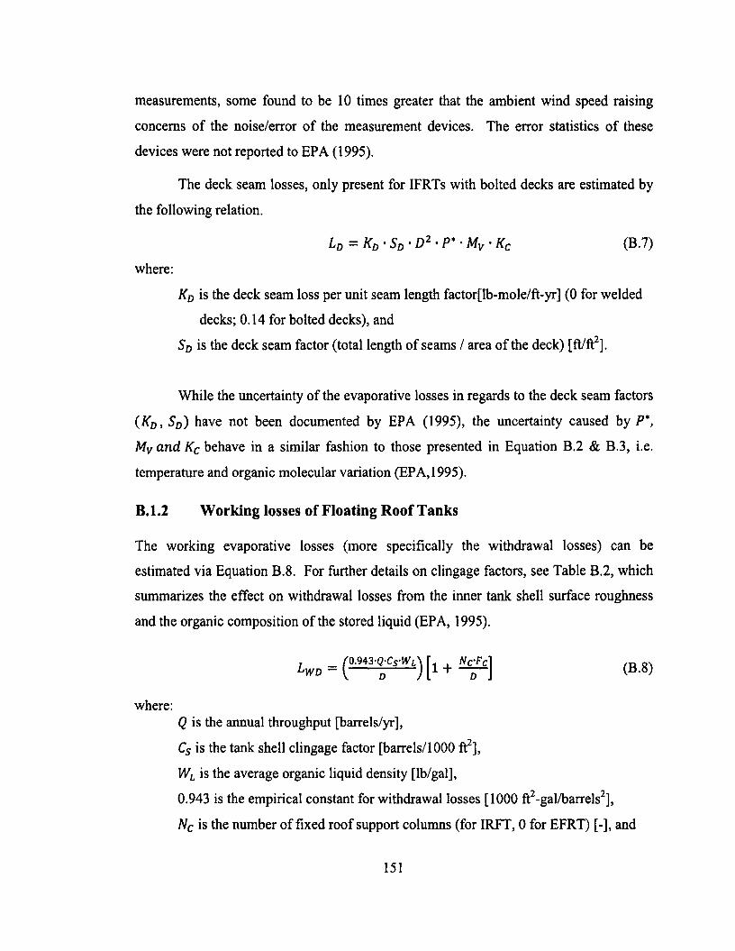
measurements, some found to be 10 times greater that the ambient wind speed raising

concerns o f the noise/error of the measurement devices. The error statistics of these

devices were not reported to EPA (1995).

The deck seam losses, only present for IFRTs with bolted decks are estimated by

the following relation.

where:

Kd is the deck seam loss per unit seam length factor[lb-mole/ft-yr] (0 for welded

decks; 0.14 for bolted decks), and

SD is the deck seam factor (total length o f seams / area o f the deck) [ft/ft2].

While the uncertainty o f the evaporative losses in regards to the deck seam factors

( KD, SD) have not been documented by EPA (1995), the uncertainty caused by P",

Mv and Kc behave in a similar fashion to those presented in Equation B.2 & B.3, i.e.

temperature and organic molecular variation (EPA, 1995).

B.1.2 W orking losses o f Floating Roof Tanks

The working evaporative losses (more specifically the withdrawal losses) can be

estimated via Equation B.8. For further details on clingage factors, see Table B.2, which

summarizes the effect on withdrawal losses from the inner tank shell surface roughness

and the organic composition o f the stored liquid (EPA, 1995).

where:Q is the annual throughput [barrels/yr],

Cs is the tank shell clingage factor [barrels/1000 ft2],

WL is the average organic liquid density [lb/gal],

0.943 is the empirical constant for withdrawal losses [1000 ft2-gal/barrels2],

Nc is the number of fixed roof support columns (for IRFT, 0 for EFRT) [-], and

Lp = KD ■ SD • D2 • P* • Mv - Kc (B.7)

(B.8)

151

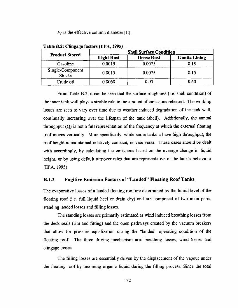
Fc is the effective column diameter [ft].

Table B.2: Clingage factors (EPA, 1995)

Product Stored Shell Surface ConditionLight Rust Dense Rust Gunite Lining

Gasoline 0.0015 0.0075 0.15Single-Component

Stocks 0.0015 0.0075 0.15

Crude oil 0.0060 0.03 0.60

From Table B.2, it can be seen that the surface roughness (i.e. shell condition) of

the inner tank wall plays a sizable role in the amount of emissions released. The working

losses are seen to vary over time due to weather induced degradation o f the tank wall,

continually increasing over the lifespan of the tank (shell). Additionally, the annual

throughput (Q) is not a full representation of the frequency at which the external floating

roof moves vertically. More specifically, while some tanks a have high throughput, the

roof height is maintained relatively constant, or vice versa. These cases should be dealt

with accordingly, by calculating the emissions based on the average change in liquid

height, or by using default turnover rates that are representative o f the tank’s behaviour

(EPA, 1995)

B.1.3 Fugitive Emission Factors o f “Landed” Floating R oof Tanks

The evaporative losses o f a landed floating roof are determined by the liquid level o f the

floating roof (i.e. full liquid heel or drain dry) and are comprised of two main parts,

standing landed losses and filling losses.

The standing losses are primarily estimated as wind induced breathing losses from

the deck seals (rim and fitting) and the open pathways created by the vacuum breakers

that allow for pressure equalization during the “landed” operating condition o f the

floating roof. The three driving mechanism are: breathing losses, wind losses and

clingage losses.

The filling losses are essentially driven by the displacement o f the vapour under

the floating roof by incoming organic liquid during the filling process. Since the total

152

time per annum the roof is said to be in the “landed” configuration is highly variable, the

estimates can only be generated on a per episode basis. In addition, the liquid level per

episode is subject to change and by that effect will change the standing loss relations that

need to be utilized in order to properly represent the emissions release per landing

episode (EPA, 1995).

The total evaporative loss from floating roof tanks during a landing episode is

given by Eq. B.9, and is essentially a summation of the standing landed losses and the

filling losses (EPA, 1995).

Ltl = Lsl + L n (B-9)

where:

Ltl is the total losses during roof landing, [lb per episode],

Lsl is the standing losses during roof landing, [lb per episode], and

Lfl is the filling losses during roof landing, [lb per episode].

As previously stated, standing losses during a roof landing are determined by the

amount of organic liquid available (i.e. either liquid heel or drain-dry) for evaporation.

For a liquid heel landed roof, the primary mechanisms are broken down into: breathing

losses, wind losses and clingage losses. For landed IFRTs, the breathing losses are

identical to those seen with fixed roof tanks. The stored organic liquid evaporates

directly into the vapour headspace (between the internal floating roof and the fixed roof)

which is contained by the breather vent. However, temperature and barometric variations

cause pressure variations that exceed the breather vent’s relief pressure (typically 0.3 psi),

resulting in breathing losses to the surroundings (EPA, 1995). Alternatively for external

floating roof tanks, temperature and pressure changes have little contribution to the total

evaporative losses when compared to the wind driven evaporative losses. The open

configuration caused by the vacuum breakers allows the wind to evacuate vapour directly

above the liquid surface (below the floating roof). The evaporative losses of landed

IFRTs and ERFTs with the liquid heel configuration can be seen in Equation B.10 and

B .ll respectively (EPA, 1995).

153

L s l - l h - i f r t - nd ' W v -V v - Ke • Ks

L s l - l h - e f r t = 0.57 - n d - D - P * * M y

(B.10)

(B. 11)

where:

L s l - l h is the daily standing evaporative losses due to wind for a landed roof with

a liquid heel [lb],

nd is the number of days that floating roof remains landed with a liquid heel

[days],

Wy is the stock vapour density [lb/ft3],

Vv is the volume of the vapour headspace [ft3],

Ke is the stock vapour expansion factor (see Equation B.12) [-],

Ks is the saturation factor [-],

D is the tank diameter [ft],

P* is the vapour pressure function [-] (see Eq. B.3 for further detail), and

My is the average molecular weight o f the liquid stock [lb/lb-mole].

where:

AT is the daily temperature operating range [°R],

T is the average temperature o f the vapour and the organic liquid [°R],

B is the empirical constant of the vapour pressure equation [°R],

P is the true vapour pressure o f the organic liquid [psia], and

PA is the average atmospheric pressure at the storage tank’s location [psia].

The evaporative losses experienced by drain-dry landed storage tanks is said to

behave in a similar fashion to clingage losses (EPA, 1995). However, the losses are

estimated as a one-time event rather than a daily event because once the storage tank is

emptied, evaporation is limited to the amount of liquid still clinging to the tank floor.

Therefore, the losses are solely estimated by the evaporation o f the “wetted” areas o f the

(B.12)

154

tank floor and thereby are proportional to the clingage factor as seen in B.8. The

equation below is used to estimate the standing losses for a drain-dry EFRT (EPA, 1995).

L s l - d d - e r f t ~ 42 ■ Cs ■ Wi ■ Area (B.13)

where:

LSl- dd is the evaporative losses due to wind for a drain-dry landed roof [lb],

42 is the conversion factor [gal/bbl],

Cs is the clingage factor [bbl/1000 ft2],

Wt is the density o f liquid [lb/gal], and

i4r e a is the surface area of the tank floor [ft2].

The filling loses of FRTs are determined by the amount o f “heavy” vapour still

present within the vapour space underneath the floating roof. The filling losses are

determined by two main things, the volume of vapour that is be displaced by the

incoming liquid to the point the roof is no longer considered “landed” and the percent of

the vapour that is saturated with vaporized hydrocarbons (EPA, 1995). The filling losses

that are associated with volume displacement are represented by CSf correction factor

presented in Equation B.15. The percent o f air that is saturated with hydrocarbons is

determined by the liquid stock available for evaporation i.e. a full liquid heel has the

highest potential for evaporation and a drain-dry tank has the lowest. To account for this

EPA (1995) utilizes the saturation factor (5 ) . Since IFRT breather vents limit the

evaporative losses to the atmosphere, the filling losses incurred by a drain-dry tank are

said to be limited by maximum saturation possible, that is seen for filling losses with a

full liquid heel, i.e. S equals 0.6 (see Equation B.14)(EPA, 1995). While this provides an

upper limit, the uncertainties for this estimation have not been presented to prove the

applicability o f this relation.

The equation below is used to estimate the filling losses for both EFRT and IFRT

(EPA, 1995).

LFL = ( ^ ) - M y C s f -S (B.14)

155

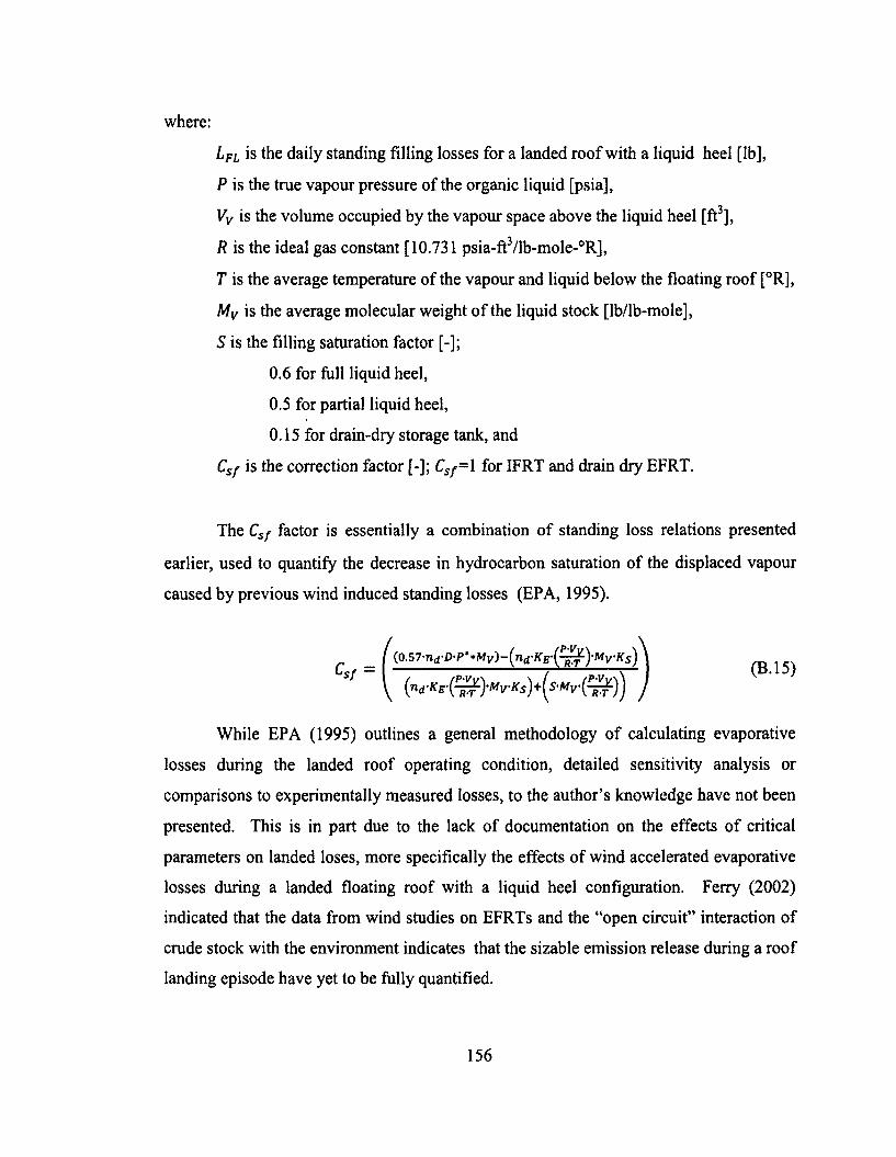
where:

Lfl is the daily standing filling losses for a landed roof with a liquid heel [lb],

P is the true vapour pressure of the organic liquid [psia],

Vv is the volume occupied by the vapour space above the liquid heel [ft3],

R is the ideal gas constant [10.731 psia-ft3/lb-mole-°R],

T is the average temperature of the vapour and liquid below the floating roof [°R],

Mv is the average molecular weight o f the liquid stock [lb/lb-mole],

S is the filling saturation factor [-];

0.6 for full liquid heel,

0.5 for partial liquid heel,

0.15 for drain-dry storage tank, and

CSf is the correction factor [-]; CSf = 1 for IFRT and drain dry EFRT.

The CSf factor is essentially a combination o f standing loss relations presented

earlier, used to quantify the decrease in hydrocarbon saturation o f the displaced vapour

caused by previous wind induced standing losses (EPA, 1995).

While EPA (1995) outlines a general methodology o f calculating evaporative

losses during the landed roof operating condition, detailed sensitivity analysis or

comparisons to experimentally measured losses, to the author’s knowledge have not been

presented. This is in part due to the lack o f documentation on the effects o f critical

parameters on landed loses, more specifically the effects o f wind accelerated evaporative

losses during a landed floating roof with a liquid heel configuration. Ferry (2002)

indicated that the data from wind studies on EFRTs and the “open circuit” interaction of

crude stock with the environment indicates that the sizable emission release during a roof

landing episode have yet to be fully quantified.

(B.15)

156

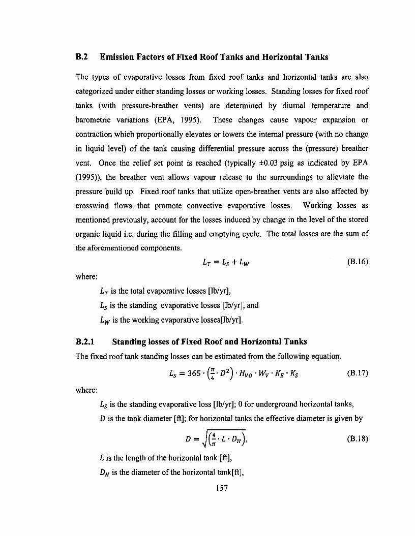
B.2 Emission Factors of Fixed Roof Tanks and Horizontal Tanks

The types o f evaporative losses from fixed roof tanks and horizontal tanks are also

categorized under either standing losses or working losses. Standing losses for fixed roof

tanks (with pressure-breather vents) are determined by diurnal temperature and

barometric variations (EPA, 1995). These changes cause vapour expansion or

contraction which proportionally elevates or lowers the internal pressure (with no change

in liquid level) o f the tank causing differential pressure across the (pressure) breather

vent. Once the relief set point is reached (typically ±0.03 psig as indicated by EPA

(1995)), the breather vent allows vapour release to the surroundings to alleviate the

pressure build up. Fixed roof tanks that utilize open-breather vents are also affected by

crosswind flows that promote convective evaporative losses. Working losses as

mentioned previously, account for the losses induced by change in the level of the stored

organic liquid i.e. during the filling and emptying cycle. The total losses are the sum of

the aforementioned components.

where:

Lt is the total evaporative losses [lb/yr],

Ls is the standing evaporative losses [lb/yr], and

Lw is the working evaporative losses[lb/yr],

B.2.1 Standing losses o f Fixed Roof and Horizontal Tanks

The fixed roof tank standing losses can be estimated from the following equation.

Ls is the standing evaporative loss [lb/yr]; 0 for underground horizontal tanks,

D is the tank diameter [ft]; for horizontal tanks the effective diameter is given by

(B.16)

(B.17)

where:

(B.18)

L is the length of the horizontal tank [ft],

Dh is the diameter o f the horizontal tank[ft],

157

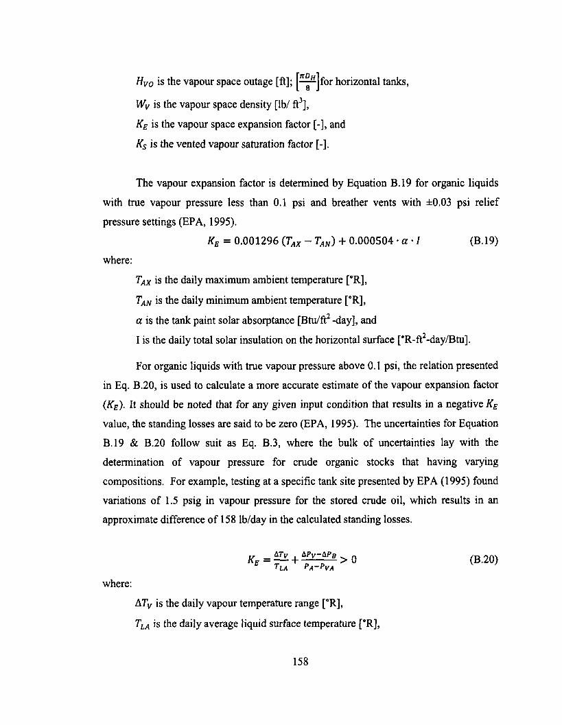
Hvo is the vapour space outage [ft]; [~ ^ ] f ° r horizontal tanks,

Wv is the vapour space density [lb/ ft3],

Ke is the vapour space expansion factor [-], and

Ks is the vented vapour saturation factor [-].

The vapour expansion factor is determined by Equation B.19 for organic liquids

with true vapour pressure less than 0.1 psi and breather vents with ±0.03 psi relief

pressure settings (EPA, 1995).

Ke = 0.001296 (Tax - Tan) + 0.000504 • a • / (B.19)

where:

Tax is the daily maximum ambient temperature [°R],

Tan is the daily minimum ambient temperature [°R],

a is the tank paint solar absorptance [Btu/ft2 -day], and

I is the daily total solar insulation on the horizontal surface [°R-ft2-day/Btu].

For organic liquids with true vapour pressure above 0.1 psi, the relation presented

in Eq. B.20, is used to calculate a more accurate estimate of the vapour expansion factor

(Ke). It should be noted that for any given input condition that results in a negative KE

value, the standing losses are said to be zero (EPA, 1995). The uncertainties for Equation

B.19 & B.20 follow suit as Eq. B.3, where the bulk of uncertainties lay with the

determination o f vapour pressure for crude organic stocks that having varying

compositions. For example, testing at a specific tank site presented by EPA (1995) found

variations o f 1.5 psig in vapour pressure for the stored crude oil, which results in an

approximate difference o f 158 lb/day in the calculated standing losses.

Ke - + *?Y_ &pb > o (B.20)T l A P A ~ P VA

where:

ATv is the daily vapour temperature range [°R],

Tla is the daily average liquid surface temperature [°R],

158

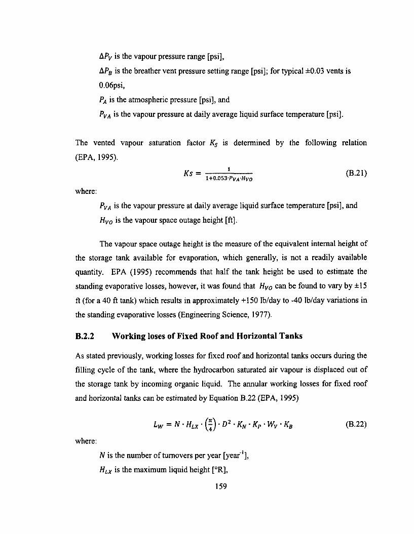
APy is the vapour pressure range [psi],

APB is the breather vent pressure setting range [psi]; for typical ±0.03 vents is

0.06psi,

PA is the atmospheric pressure [psi], and

PVA is the vapour pressure at daily average liquid surface temperature [psi].

The vented vapour saturation factor Ks is determined by the following relation

(EPA, 1995).

Ks = ------------------- (B.21)1+ 0.053 - P v a - H v O

where:

PVA is the vapour pressure at daily average liquid surface temperature [psi], and

Hvo is the vapour space outage height [ft].

The vapour space outage height is the measure o f the equivalent internal height of

the storage tank available for evaporation, which generally, is not a readily available

quantity. EPA (1995) recommends that half the tank height be used to estimate the

standing evaporative losses, however, it was found that Hv0 can be found to vary by ±15

ft (for a 40 ft tank) which results in approximately +150 lb/day to -40 lb/day variations in

the standing evaporative losses (Engineering Science, 1977).

B.2.2 W orking loses o f Fixed Roof and Horizontal Tanks

As stated previously, working losses for fixed roof and horizontal tanks occurs during the

filling cycle of the tank, where the hydrocarbon saturated air vapour is displaced out of

the storage tank by incoming organic liquid. The annular working losses for fixed roof

and horizontal tanks can be estimated by Equation B.22 (EPA, 1995)

Lw = N • Hlx • g ) • D 2 • Kn ■ KP • Wv ■ KB (B.22)

where:

N is the number o f turnovers per year [year'1],

Hlx is the maximum liquid height [°R],

159

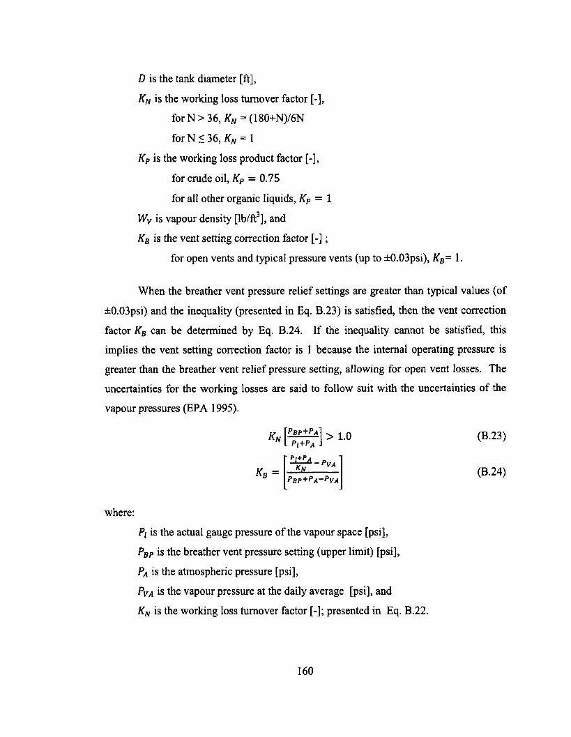
D is the tank diameter [ft],

Kn is the working loss turnover factor [-],

for N > 36, Kn = (180+N)/6N

for N < 36, K/v = 1

KP is the working loss product factor [-],

for crude oil, KP = 0.75

for all other organic liquids, KP = 1

Wv is vapour density [lb/ft3], and

Kb is the vent setting correction factor [-];

for open vents and typical pressure vents (up to ±0.03psi), KB= 1.

When the breather vent pressure relief settings are greater than typical values (of

±0.03psi) and the inequality (presented in Eq. B.23) is satisfied, then the vent correction

factor Kb can be determined by Eq. B.24. If the inequality cannot be satisfied, this

implies the vent setting correction factor is 1 because the internal operating pressure is

greater than the breather vent relief pressure setting, allowing for open vent losses. The

uncertainties for the working losses are said to follow suit with the uncertainties o f the

vapour pressures (EPA 1995).

K" f i ^ r l > 1-° (B-23)

K„ =P b P + P A ~ P VA

(B.24)

where:

Pj is the actual gauge pressure o f the vapour space [psi],

PBP is the breather vent pressure setting (upper limit) [psi],

PA is the atmospheric pressure [psi],

PVA is the vapour pressure at the daily average [psi], and

Kn is the working loss turnover factor [-]; presented in Eq. B.22.

160

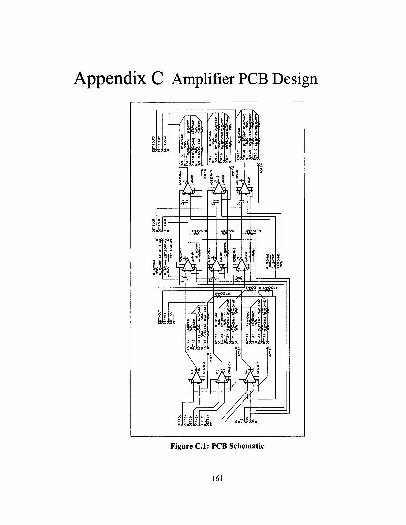
Appendix C Amplifier PCB Design

S f f i

I I I

/ M

Figure C.l: PCB Schematic

161

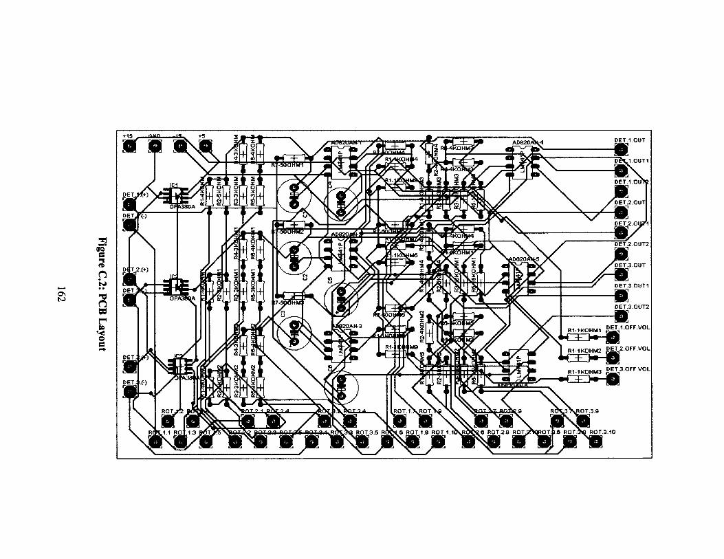
Dl T2X+)

AP82UAN-T A D 8 2 0 j

D EC1.0U T1

D ET.2.0U T2

.3.0UT1

DET.3.0U T2

120 AN-3R1-1KOHM1 g i i j

I R1-1KOHM2 g U - :

k a 3 H HR1-1KOHM3 q £ I h:

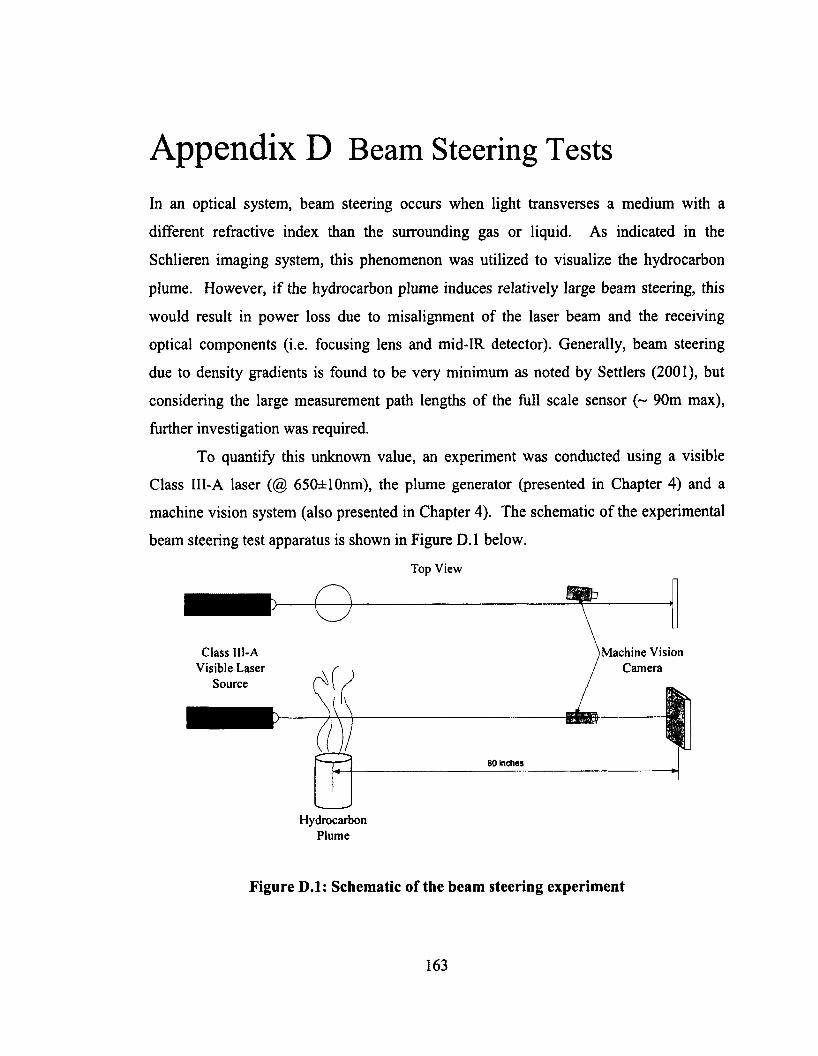
Appendix D Beam Steering TestsIn an optical system, beam steering occurs when light transverses a medium with a

different refractive index than the surrounding gas or liquid. As indicated in the

Schlieren imaging system, this phenomenon was utilized to visualize the hydrocarbon

plume. However, if the hydrocarbon plume induces relatively large beam steering, this

would result in power loss due to misalignment of the laser beam and the receiving

optical components (i.e. focusing lens and mid-IR detector). Generally, beam steering

due to density gradients is found to be very minimum as noted by Settlers (2001), but

considering the large measurement path lengths of the full scale sensor (~ 90m max),

further investigation was required.

To quantify this unknown value, an experiment was conducted using a visible

Class III-A laser (@ 650±10nm), the plume generator (presented in Chapter 4) and a

machine vision system (also presented in Chapter 4). The schematic o f the experimental

beam steering test apparatus is shown in Figure D .l below.

Top View

eClass III-A

Visible Laser Source

Machine Vision Camera

80 Inches

HydrocarbonPlume

Figure D.l: Schematic of the beam steering experiment

163

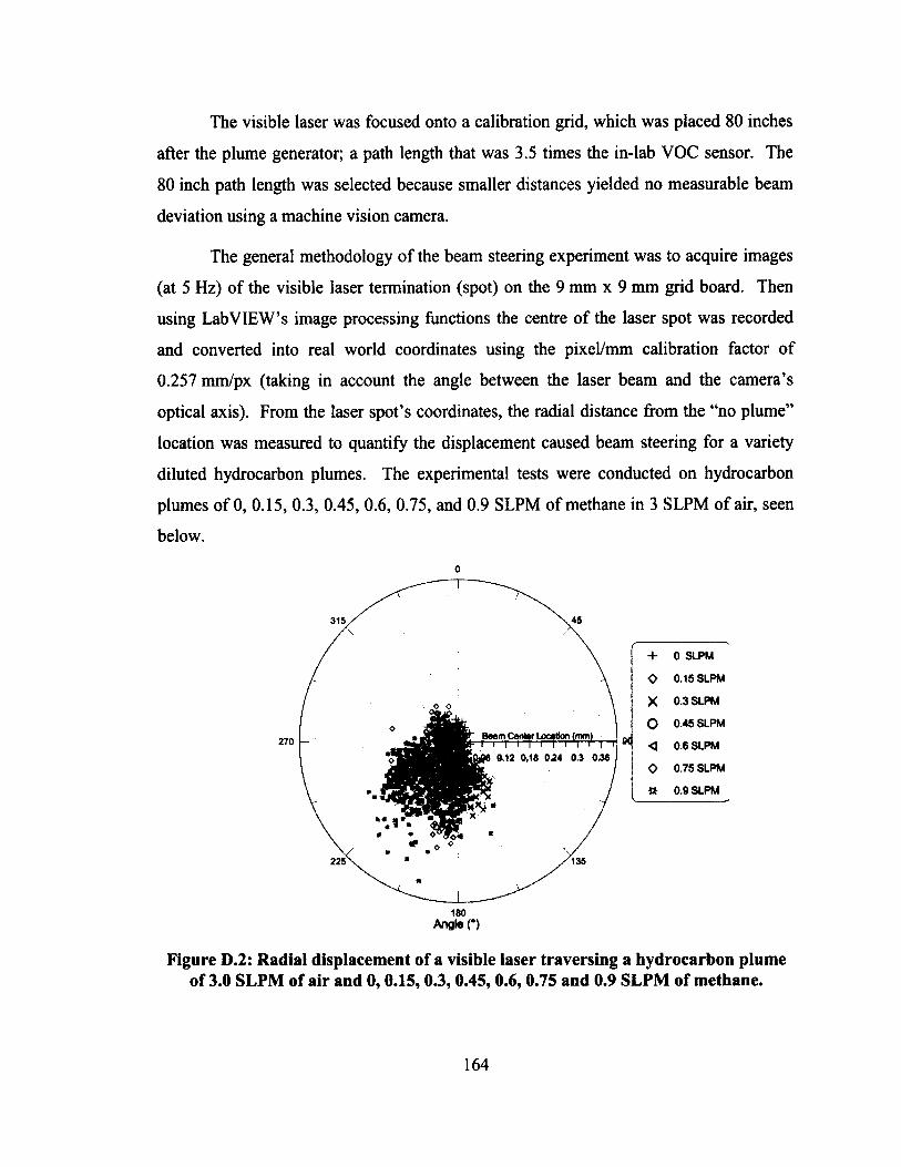
The visible laser was focused onto a calibration grid, which was placed 80 inches

after the plume generator; a path length that was 3.5 times the in-lab VOC sensor. The

80 inch path length was selected because smaller distances yielded no measurable beam

deviation using a machine vision camera.

The general methodology of the beam steering experiment was to acquire images

(at 5 Hz) o f the visible laser termination (spot) on the 9 mm x 9 mm grid board. Then

using Lab VIEW’S image processing functions the centre o f the laser spot was recorded

and converted into real world coordinates using the pixel/mm calibration factor o f

0.257 mm/px (taking in account the angle between the laser beam and the camera’s

optical axis). From the laser spot’s coordinates, the radial distance from the “no plume”

location was measured to quantify the displacement caused beam steering for a variety

diluted hydrocarbon plumes. The experimental tests were conducted on hydrocarbon

plumes o f 0, 0.15, 0.3, 0.45, 0.6, 0.75, and 0.9 SLPM of methane in 3 SLPM of air, seen

below.

+ 0 SLPM

O 0.15 SLPM

X 0.3 SLPM

O 0.45 SLPM

< 0.6 SLPM

O 0.75 SLPM

tt 0.9 SLPMV___________________________.

Figure D.2: Radial displacement of a visible laser traversing a hydrocarbon plume of 3.0 SLPM of air and 0,0.15,0.3,0.45,0.6,0.75 and 0.9 SLPM of methane.

B eam 1t - t - t

180 Angle (°)

164

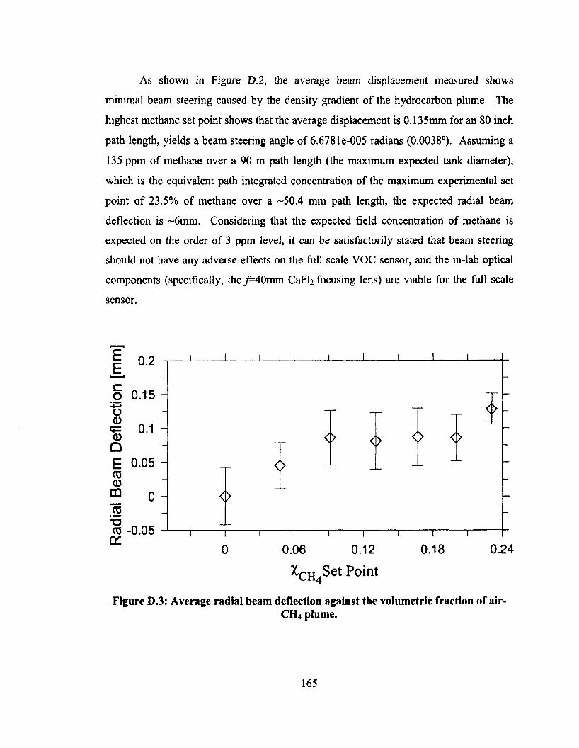
As shown in Figure D.2, the average beam displacement measured shows

minimal beam steering caused by the density gradient o f the hydrocarbon plume. The

highest methane set point shows that the average displacement is 0.135mm for an 80 inch

path length, yields a beam steering angle of 6.6781e-005 radians (0.0038°). Assuming a

135 ppm of methane over a 90 m path length (the maximum expected tank diameter),

which is the equivalent path integrated concentration o f the maximum experimental set

point o f 23.5% of methane over a -50.4 mm path length, the expected radial beam

deflection is ~6mm. Considering that the expected field concentration of methane is

expected on the order o f 3 ppm level, it can be satisfactorily stated that beam steering

should not have any adverse effects on the full scale VOC sensor, and the in-lab optical

components (specifically, the j= 40mm CaF^ focusing lens) are viable for the full scale

sensor.

| 0.2 -

O 0.15 -0

% 0 1 OE 0.050om o to

0 -0.05 fZ 0.240.180.06 0.120

XCH4 Set Point

Figure D.3: Average radial beam deflection against the volumetric fraction of air-CH4 plume.

165

Documents

NOVEL ECONOMICAL EMISSION MONITORING · PDF fileYour file Votre reference ISBN: 978-0-494-93511-8 ... 4.2.1 Lasing Assembly ... 4.2.2 Test GasDelivery System