1

Nouriel Roubini and David Backus

MBA Lectures in Macroeconomics

http://people.stern.nyu.edu/nroubini/LNOTES.HTM

Part I. Overview of the World Economy

Chapter 1: Monitoring Macroeconomic Performance

Chapter 2: Business Cycle and Financial Indicators

Chapter 3: International Indicators

Chapter 4: Productivity and Growth

Part II. The Classical Theory of the Long-Run

Chapter 5: Output and Real Interest Rates

Chapter 6: Money and Inflation

Chapter 7: Exchange Rates

Part III. The Keynesian Theory of the Short-Run

(Incomplete. Missing Part III chapters will distributed in class and available online in the

near future).

8. Money, Interest Rates and Exchange Rates. Fixed and Flexible Exchange Rate Regimes.TheAsian Crisis of 1997

9. IS/LM Model in a Closed Economy

10. IS/LM Model in an Open Economy

11. Fiscal Policy

12. Monetary Policy and Commercial Banking

Copyright: Nouriel Roubini and David Backus, Stern School of Business, NYU, 1998.

2

Chapter 1: Monitoring Macroeconomic Performance

Growth and Business Cycles

Gross Domestic Product

Accounting Identities

The Current Account

Current Account Deficits and Foreign Debt Accumulation: A preview of the Asian crisis

What Causes Current Account Deficits? Are Such Deficits Bad?

Prices and "Real'' Quantities

Summary

Further Readings

Further Web Links and Readings

Growth and Business Cycles

The two central issues of macroeconomics are evident in Figure 1, time series graph of real

GDP (Gross Domestic Product) in the US over the last forty years. As we'll see shortly, GDP

is a measure of total production of goods and services in an economy, the US being one

example. The two obvious features of postwar GDP are its upward trend (GDP has generally

been increasing over the postwar period) and the short-term fluctuations or "wiggles'' in this

generally upward-sloping line. We refer to these two issues as economic growth and business

cycles, respectively. When you look at data over periods this long, the wiggles don't look

very important, and in a sense they aren't: the short-term fluctuations are a small part of the

wealth of nations. But from a personal point of view these cycles can be very important, as

businessmen and workers dealing with the latest 2001 recession could tell you. We'll look at

both growth and cycles in this course.

The classical question of economic growth is why some countries are richer and/or grow

faster than others. (The two are clearly related, since countries that grow faster will

eventually be richer.) Some examples are given in Figure 2, which graphs per capita GDP for

three countries over the postwar period. [All are measured in 1980 US dollars.] This figure

differs from the previous one, since I've expressed output in per capita (per person) terms by

dividing GDP by population. This produces a more meaningful comparison between countries, since countries with more people don't automatically have higher numbers.

Figure 2 illustrates a number of differences among three countries: Japan, Argentina, and the

US. Perhaps the most obvious feature is that the US is the richest country: by this measure in

1985, it was 30 percent richer than Japan and almost three times as rich as Argentina. These

are averages so they ignore a lot of differences at the individual level, but they give you some

idea of where these nations stand economically. The comparison with Argentina gives us an

idea of the enormous differences between rich and poor countries. In fact, Argentineans are

relatively well off, roughly five times better off than an average person in India. But the truly

remarkable country is Japan. In 1913 Argentina was about 3 times richer than Japan, now it's

the opposite. Japan's remarkable performance has lasted, thus far, for over a century.

Argentina, on the other hand, has gone from one of the richest countries in the world at the

turn of the century to an average Latin American country economically that experienced a

severe economic and financial crisis in 2001.

3

Figure 3 does the same thing for the US, China, and Korea, where again we see sharp

differences between countries. China used to be one of the poorest of these countries but for

the last 20 years China has been among the most rapidly growing countries in the world.

Combined with China's enormous population, some estimates suggest that China is now the world's third largest market.

These comparisons are so striking I find it hard to leave them, but let's turn our attention to

the other aspect of macroeconomics, business cycles. From a business point of view these

short-term movements in the economy are of more immediate concern. You may want to

know, for example, whether the economy will be in better shape when you finish your degree

or whether your airline stock is going to be worth anything in 12 months (airlines are

notoriously sensitive to recessions). You get a much better picture of the short-term fluctuations in Figure 4, where we graph annual growth rates of US GDP.

By annual growth rate, I mean the "year-on-year'' growth rate in quarterly data,

(GDPt - GDPt-4) /GDPt-4

where GDPt is GDP in quarter t (for example the third quarter of 2005) and GDPt-4 is GDP

four quarters before (for example the third quarter of 2004). Viewed from this perspective,

the short-term movements seem a lot bigger than they did in Figure 1. For the postwar period

as a whole the average growth rate of 3.3 percent per year is swamped by the year-to-year

variations. [Statistically, we could say that the mean of 3.3 percent per year is only slightly

larger than the standard deviation of 3.0 percent. A plus or minus two standard deviation

interval is thus (-2.7,9.3). If you find this mysterious, review your statistics notes.] The nine

downward spikes, all of which touch or pass the axis, are the nine postwar recessions, defined

most simply as two consecutive quarters of declining GDP. The National Bureau of

Economic Research, the de facto arbiter of business cycles in the US, has decided that the

troughs (the bottom point) of these recessions occurred in November 1949, May 1954, April

1958, February 1961, November 1970, March 1975, July 1980, November 1982, April 1992 and November 2001.

Note that in Figure 4 the growth rate of GDP is defined as year-on-year growth rate of

quarterly GDP. Note that there is an alternative way to define the growth rate of the

economy: this is the way the growth rate of GDP is usually reported by the US Government

and the press. It consists of measuring the growth rate of GDP in a particular quarter relative

to the previous quarter and annualize such quarterly rate of growth by multiplying by four. Accordingly, the quarterly growth rate of the economy at an annual rate (AR) is:

4 x [(GDPt - GDPt-1) /GDPt-1 ]

Figure 4' shows the growth rate of GDP according to this alternative measure. As a

comparison of figures 4 and 4' shows, the second way of expressing the growth rate of the

economy implies a greater volatility of output growth as quarterly changes in the rates of

growth are amplified when measured at annualized rates. As the annualized quarterly growth

rate gives a better measure of the very recent performance of the economy, this is the

measure usually reported in the press and most closely analyzed in the business and financial

sector. However, the year-on-year definition gives a better measure of the growth rate of the

4

economy over a longer period, i.e. how the economy has actually grown over the last 4

quarters. A similar distinction between year-on-year growth rate and annualized quarterly

growth rate holds for the other macroeconomic variables. To create quick charts of macro

variables using these alternative definitions, you can use the Economic Chart Dispenser

available on the Web. Tables with the most recent GDP data is available from the Bureau of

Economic Analysis at the Department of Commerce. For more information on specific

macroeconomic variables see the course homepage on the Hyptertext Glossary of Business Cycle Indicators.

One question you might ask is why the economy experiences such large short-term

fluctuations. We'll return to this later in the course. For now let me just say that recessions

happen: business cycles have been a property of all economies for as long as we've had data

and, despite what politicians tell us, they show no sign of going away. You can see signs of

cycles in other countries in Figure 5. In Figure 5 I report growth rates of real GNP (total, not

per capita) in Germany and Japan, where we see that they, too, have had substantial

fluctuations, despite their higher average growth rates. For Japan, though, there would be

only recessions between World War II and 1990 if we defined a recession, as is typically

done in the US, as negative growth. Note, however, that in the 1990s, Japan experience a

period of protracted economic stagnation. The average growth rate per year was close to zero

between 1992 and 1995. Growth recovered in 1996 but such recovery fizzled in 1997 when

the economy went again into a slump. The weak economic performance of Japan in the 1990s

and 1997 in particular contributed to exacerbate the 1997 economic crisis in East Asia: as

Japan is a leading export market for many East Asian countries, the stagnation of growth in

Japan in this decade led to a reduction (since 1995) in the export growth rate of many East Asian countries.

Gross Domestic Product

Today we're going to go behind the scenes, as it were, and review some of the measurement

issues that lie behind concepts like GDP and GNP. The goal is to gain some familiarity with

the most important macroeconomic indicators so that we know something about their

meanings, strengths, and weaknesses. We'll start with an accounting system analogous to the

income statement used by firms: the National Income and Product Accounts (NIPA)

constructed by the Bureau of Economic Analysis at the Department of Commerce. In many

respects this system is like financial accounting systems for firms and, in fact, relies heavily

on reports made by individual firms to the government. It's also like firm accounting in that

one needs to use some artistry to make sense of the numbers.

Our first goal is a measure of overall production, which we will refer to as Gross Domestic

Product, or GDP. Gross National Product, or GNP, is closely related. Both are measures of

the total production of goods and services of the US economy for a particular time period---

say, the year 2004 or the first quarter of 2005 (January through March). We will discuss below the difference between these two measures.

We can think of total production in the US as the sum of production by all the individual

firms, but there's a subtlety here that we can illustrate with a simple example. Consider a firm

that assembles PCs from parts made in Taiwan. Its only other expenses are labor. Let's say

that the firm's income statement looks something like this:

5

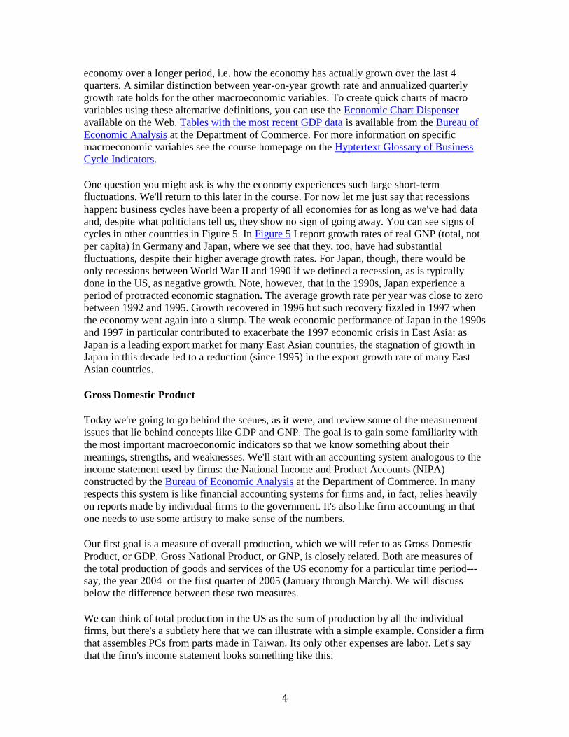
Sales revenue 40,000,000

Expenses 26,000,000

Wages 20,000,000

Cost of Parts 6,000,000

Net Income 14,000,000

The question is how we measure this firm's contribution to US output. The straightforward

answer is 40m, the total value of its sales. But if we think about this a minute we realize that

6m of this was produced somewhere else, so it shouldn't be counted as part of the firm's---or

the US's---output. A better answer is 34m, the amount of value the firm has added to the

imported parts. This principle is applied throughout the NIPA: we take value-added by

everyone in the economy and add it up to get GDP. When we sum across firms, we only

count the value added by each one. US GDP is total value-added for the US economy.

Another way to compute value-added is to sum payments to labor and capital. In this case we

add 20m paid to workers to 14m profit that goes to owners of the firm---capital. That gives us

factor payments of 34m, the same number we found above using a different method, factor being a term used by economists to mean inputs

The term value-added has the connotation that the prices that underlie the firm's income

statement reflect economic value in some deeper sense. When we compared the GDP's of

three countries earlier we presumed that the country with the larger per capita GDP was

richer in some useful sense. But suppose they produce different goods. Suppose country A

produces 10 billion apples and country B produces 10 billion bananas. Which is richer? We

generally assume that if apples are worth more than bananas then country A is richer. The

idea is that market prices tell us which is more valuable, apples or bananas. The same thing

underlies our measurement of value-added. Suppose, to make this concrete, that the 40m

sales of our fictitious company was 20,000 PCs at $2,000 each. Our presumption is that the

market price of $2,000 reflects economic value and we use it as part of our calculation of

GDP. In some cases this isn't so easy. In, say, North Korea (or until recently, China), prices

do not generally reflect market forces, so it's not easy to calculate economic values. There are

also some subtle issues in market economies about how to value nonmarket activities like

government spending, housework, pollution, and so on.

I promised a little while ago to mention the difference between GDP and GNP. GDP is, to

me, the more natural concept. It measures total value-added produced by firms operating in

the US. GNP, on the other hand, measures value-added generated by factor inputs, capital

and labor, owned by Americans. This is slightly different because there are foreign factors

(labor and capital) producing in the US and American factors producing abroad. Here's a

concrete example. An American working in London for Goldman Sachs would count in US

GNP but not US GDP. She would also count in British GDP, since she's working there.

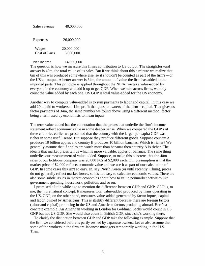
To clarify the distinction between GDP and GDP take the following example. Suppose that

the firm we considered before is partly owned by Japanese owners. Let us also assume that

some of the workers in the firm are Japanese managers temporarily working in the U.S. Then:

6

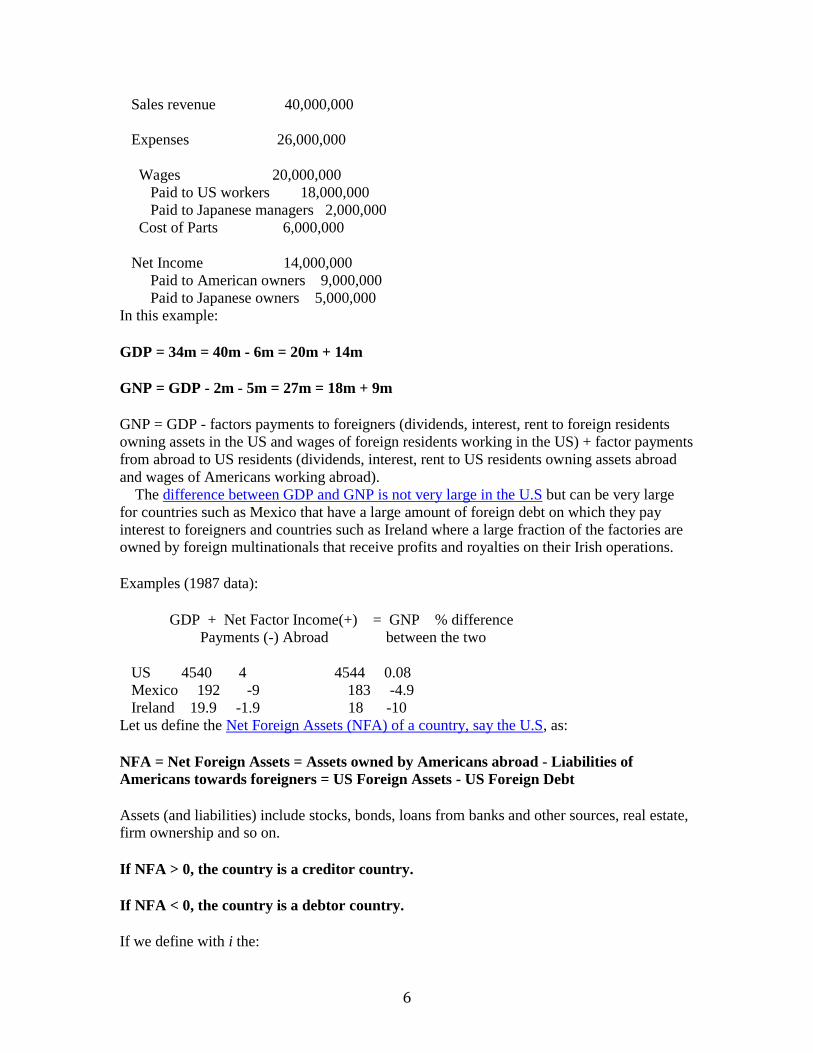
Sales revenue 40,000,000

Expenses 26,000,000

Wages 20,000,000

Paid to US workers 18,000,000

Paid to Japanese managers 2,000,000

Cost of Parts 6,000,000

Net Income 14,000,000

Paid to American owners 9,000,000

Paid to Japanese owners 5,000,000

In this example:

GDP = 34m = 40m - 6m = 20m + 14m

GNP = GDP - 2m - 5m = 27m = 18m + 9m

GNP = GDP - factors payments to foreigners (dividends, interest, rent to foreign residents

owning assets in the US and wages of foreign residents working in the US) + factor payments

from abroad to US residents (dividends, interest, rent to US residents owning assets abroad

and wages of Americans working abroad).

The difference between GDP and GNP is not very large in the U.S but can be very large

for countries such as Mexico that have a large amount of foreign debt on which they pay

interest to foreigners and countries such as Ireland where a large fraction of the factories are owned by foreign multinationals that receive profits and royalties on their Irish operations.

Examples (1987 data):

GDP + Net Factor Income(+) = GNP % difference

Payments (-) Abroad between the two

US 4540 4 4544 0.08

Mexico 192 -9 183 -4.9

Ireland 19.9 -1.9 18 -10

Let us define the Net Foreign Assets (NFA) of a country, say the U.S, as:

NFA = Net Foreign Assets = Assets owned by Americans abroad - Liabilities of

Americans towards foreigners = US Foreign Assets - US Foreign Debt

Assets (and liabilities) include stocks, bonds, loans from banks and other sources, real estate, firm ownership and so on.

If NFA > 0, the country is a creditor country.

If NFA < 0, the country is a debtor country.

If we define with i the:

7

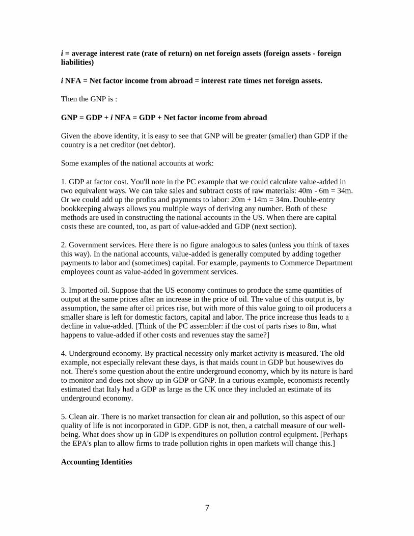
i = average interest rate (rate of return) on net foreign assets (foreign assets - foreign

liabilities)

i NFA = Net factor income from abroad = interest rate times net foreign assets.

Then the GNP is :

GNP = GDP + i NFA = GDP + Net factor income from abroad

Given the above identity, it is easy to see that GNP will be greater (smaller) than GDP if the country is a net creditor (net debtor).

Some examples of the national accounts at work:

1. GDP at factor cost. You'll note in the PC example that we could calculate value-added in

two equivalent ways. We can take sales and subtract costs of raw materials: 40m - 6m = 34m.

Or we could add up the profits and payments to labor: 20m + 14m = 34m. Double-entry

bookkeeping always allows you multiple ways of deriving any number. Both of these

methods are used in constructing the national accounts in the US. When there are capital

costs these are counted, too, as part of value-added and GDP (next section).

2. Government services. Here there is no figure analogous to sales (unless you think of taxes

this way). In the national accounts, value-added is generally computed by adding together

payments to labor and (sometimes) capital. For example, payments to Commerce Department employees count as value-added in government services.

3. Imported oil. Suppose that the US economy continues to produce the same quantities of

output at the same prices after an increase in the price of oil. The value of this output is, by

assumption, the same after oil prices rise, but with more of this value going to oil producers a

smaller share is left for domestic factors, capital and labor. The price increase thus leads to a

decline in value-added. [Think of the PC assembler: if the cost of parts rises to 8m, what happens to value-added if other costs and revenues stay the same?]

4. Underground economy. By practical necessity only market activity is measured. The old

example, not especially relevant these days, is that maids count in GDP but housewives do

not. There's some question about the entire underground economy, which by its nature is hard

to monitor and does not show up in GDP or GNP. In a curious example, economists recently

estimated that Italy had a GDP as large as the UK once they included an estimate of its

underground economy.

5. Clean air. There is no market transaction for clean air and pollution, so this aspect of our

quality of life is not incorporated in GDP. GDP is not, then, a catchall measure of our well-

being. What does show up in GDP is expenditures on pollution control equipment. [Perhaps the EPA's plan to allow firms to trade pollution rights in open markets will change this.]

Accounting Identities

8

By the magic of double entry bookkeeping, we can divide GDP up in a number of ways. This

will give us several identities that will reappear in different guises throughout the course.

The first is to think of value-added as payments to labor and capital. The point is that sales

revenue shows up as income to someone. Intermediate goods are income to the firm that

makes them, wages are income to workers, and profits are income to the people who own the

firm. As a result, we can think of GDP as measuring either income or output: the two numbers are the same thing.

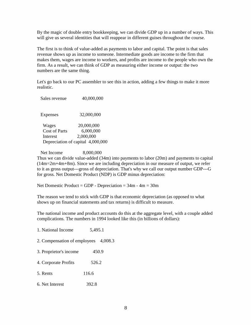
Let's go back to our PC assembler to see this in action, adding a few things to make it more realistic.

Sales revenue 40,000,000

Expenses 32,000,000

Wages 20,000,000

Cost of Parts 6,000,000

Interest 2,000,000

Depreciation of capital 4,000,000

Net Income 8,000,000

Thus we can divide value-added (34m) into payments to labor (20m) and payments to capital

(14m=2m+4m+8m). Since we are including depreciation in our measure of output, we refer

to it as gross output---gross of depreciation. That's why we call our output number GDP---G

for gross. Net Domestic Product (NDP) is GDP minus depreciation:

Net Domestic Product = GDP - Depreciation = 34m - 4m = 30m

The reason we tend to stick with GDP is that economic depreciation (as opposed to what

shows up on financial statements and tax returns) is difficult to measure.

The national income and product accounts do this at the aggregate level, with a couple added

complications. The numbers in 1994 looked like this (in billions of dollars):

1. National Income 5,495.1

2. Compensation of employees 4,008.3

3. Proprietor's income 450.9

4. Corporate Profits 526.2

5. Rents 116.6

6. Net Interest 392.8

9

This is basically the same thing we did for the firm. Line 2 is labor expenses, lines 4 are

corporate profits, line 3 is a combination (for unincorporated businesses, like farmers and

doctors, it's not easy to separate labor and capital expenses). On average, about 60-70 percent

of gross output goes to labor, the rest to capital (including corporate profits, rents, net interest

and proprietor's income). The point is that GDP measures both production of goods and

services and income to workers and owners: by the logic of double entry bookkeeping, the

two are inseparable.

Our second look at GDP comes from the perspective of purchases of final goods: who buys

them (consumers, firms, governments, or foreigners). The most common decomposition of this sort is

GDP = consumer expenditures + investment + government purchases of goods and

services + net exports,

or, in a more compact notation,

GDP = C + I + G + NX.

Net exports is simply exports (X) minus imports (M) or NX = X - M. Net exports are also

referred to as the trade balance. Consumption is expenditures on consumer goods by

households. Investment in this course will always mean accumulation of physical capital:

purchases of new buildings and machines, plant and equipment in the language of national

income accountants (a close relative of the beloved PPE of financial accounting). It also

includes accumulation of inventories (that is, the change in stocks of inventories).

Government consumption here consists of purchases of goods and services (mainly wages)

and does not include government outlays for social security, unemployment insurance, or

interest on the debt. We think of these, instead, as transfers, since no goods or services are

involved. We'll see more of this when we look at the government deficit. U.S. data on the

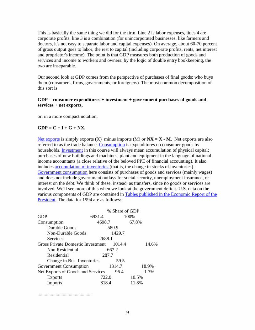
various components of GDP are contained in Tables published in the Economic Report of the President. The data for 1994 are as follows:

% Share of GDP

GDP 6931.4 100%

Consumption 4698.7 67.8%

Durable Goods 580.9

Non-Durable Goods 1429.7

Services 2688.1

Gross Private Domestic Investment 1014.4 14.6%

Non Residential 667.2

Residential 287.7

Change in Bus. Inventories 59.5

Government Consumption 1314.7 18.9%

Net Exports of Goods and Services -96.4 -1.3%

Exports 722.0 10.5%

Imports 818.4 11.8%

.............................................

10

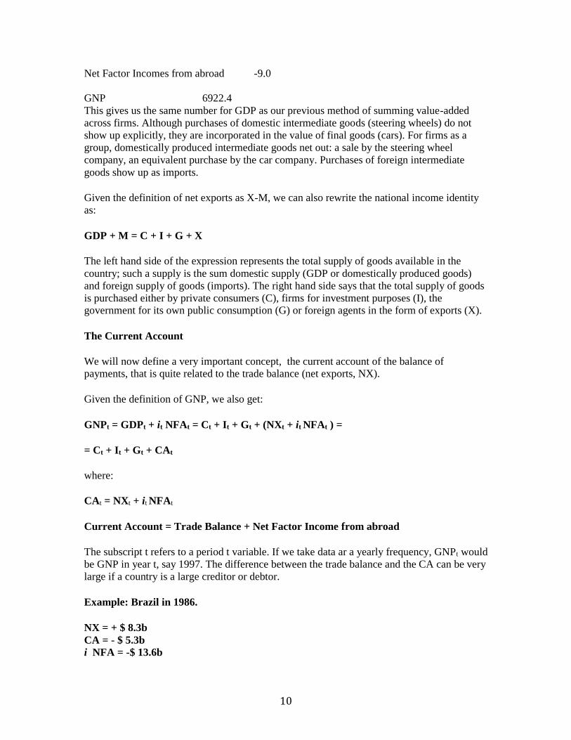
Net Factor Incomes from abroad -9.0

GNP 6922.4

This gives us the same number for GDP as our previous method of summing value-added

across firms. Although purchases of domestic intermediate goods (steering wheels) do not

show up explicitly, they are incorporated in the value of final goods (cars). For firms as a

group, domestically produced intermediate goods net out: a sale by the steering wheel

company, an equivalent purchase by the car company. Purchases of foreign intermediate

goods show up as imports.

Given the definition of net exports as X-M, we can also rewrite the national income identity

as:

GDP + M = C + I + G + X

The left hand side of the expression represents the total supply of goods available in the

country; such a supply is the sum domestic supply (GDP or domestically produced goods)

and foreign supply of goods (imports). The right hand side says that the total supply of goods

is purchased either by private consumers (C), firms for investment purposes (I), the government for its own public consumption (G) or foreign agents in the form of exports (X).

The Current Account

We will now define a very important concept, the current account of the balance of payments, that is quite related to the trade balance (net exports, NX).

Given the definition of GNP, we also get:

GNPt = GDPt + it NFAt = Ct + It + Gt + (NXt + it NFAt ) =

= Ct + It + Gt + CAt

where:

CAt = NXt + it NFAt

Current Account = Trade Balance + Net Factor Income from abroad

The subscript t refers to a period t variable. If we take data ar a yearly frequency, GNPt would

be GNP in year t, say 1997. The difference between the trade balance and the CA can be very

large if a country is a large creditor or debtor.

Example: Brazil in 1986.

NX = + $ 8.3b

CA = - $ 5.3b i NFA = -$ 13.6b

11

In this example, Brazil had in 1986 a large current account deficit in spite of a trade surplus.

In fact, Brazil was a heavy foreign debtor, having borrowed a lot in the 1970s and 1980s. By

1986 the total foreign debt of Brazil was above $100b and the net foreign interest payments

on that debt (and profit repatriations of foreign firms owning assets in Brazil) equaled $13.6b.

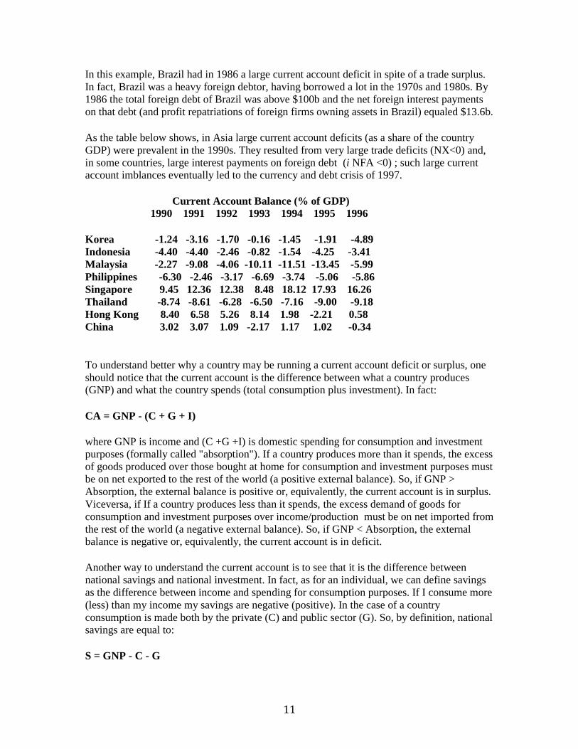
As the table below shows, in Asia large current account deficits (as a share of the country

GDP) were prevalent in the 1990s. They resulted from very large trade deficits (NX<0) and,

in some countries, large interest payments on foreign debt (i NFA <0) ; such large current account imblances eventually led to the currency and debt crisis of 1997.

Current Account Balance (% of GDP) 1990 1991 1992 1993 1994 1995 1996

Korea -1.24 -3.16 -1.70 -0.16 -1.45 -1.91 -4.89

Indonesia -4.40 -4.40 -2.46 -0.82 -1.54 -4.25 -3.41

Malaysia -2.27 -9.08 -4.06 -10.11 -11.51 -13.45 -5.99

Philippines -6.30 -2.46 -3.17 -6.69 -3.74 -5.06 -5.86

Singapore 9.45 12.36 12.38 8.48 18.12 17.93 16.26

Thailand -8.74 -8.61 -6.28 -6.50 -7.16 -9.00 -9.18

Hong Kong 8.40 6.58 5.26 8.14 1.98 -2.21 0.58

China 3.02 3.07 1.09 -2.17 1.17 1.02 -0.34

To understand better why a country may be running a current account deficit or surplus, one

should notice that the current account is the difference between what a country produces (GNP) and what the country spends (total consumption plus investment). In fact:

CA = GNP - (C + G + I)

where GNP is income and (C +G +I) is domestic spending for consumption and investment

purposes (formally called "absorption"). If a country produces more than it spends, the excess

of goods produced over those bought at home for consumption and investment purposes must

be on net exported to the rest of the world (a positive external balance). So, if GNP >

Absorption, the external balance is positive or, equivalently, the current account is in surplus.

Viceversa, if If a country produces less than it spends, the excess demand of goods for

consumption and investment purposes over income/production must be on net imported from

the rest of the world (a negative external balance). So, if GNP < Absorption, the external balance is negative or, equivalently, the current account is in deficit.

Another way to understand the current account is to see that it is the difference between

national savings and national investment. In fact, as for an individual, we can define savings

as the difference between income and spending for consumption purposes. If I consume more

(less) than my income my savings are negative (positive). In the case of a country

consumption is made both by the private (C) and public sector (G). So, by definition, national savings are equal to:

S = GNP - C - G

12

Substituting this definition of savings in the expression for the current account, we get:

CA = S - I

To see why the current account is equal to the difference between savings and investment,

consider the similarity of a country with an individual. For simplicity, suppose initially that

the investment of the individual is zero and that G=0. If an individual consumes (C) more

than his/her income (GNP), the savings (S=GNP-C) of the individual will be negative (S<0).

Since the individual investment is zero, the current account of the individual will be equal to

his/her savings (CA=S<0). So, an individual with negative savings has a deficit in its current

account. In a similar way, if I=0, a country running a current account deficit is consuming

(including both public and private consumption) more than it is producing as CA = S = GNP-

C-G.

Consider now how positive investment (I>0) changes things. Take again the case of an

individual who has now positive savings (S=GNP-C >0). Suppose now that the individual

makes real investments; for example, he/she may buy a new home (residential investment).

Suppose that the investment in the new home is greater than the savings of the individual (I >

S) as it is usually the case. In this case the current account of the individual is in deficit as CA

= S - I <0. Since the income of the individual (GNP) is less than his/her total spending (for

consumption and investment), the individual current account is in deficit, or the individual's

savings are below the individual's investment. The same story holds for a country. If a

country invests more than its saves, the country is producing an amount of output/income

(GNP) that smaller than the total spending on goods for consumption and investment

purposes (C+G+I). Therefore, the excess of spending (absorption) over income or,

equivalently, the excess of investment over savings implies that the country is running a current account deficit.

Insight in the Asian economic crisis: Why current account deficits lead to the

accumulation of a large stock of foreign debt.

It is very important to understand that if a country runs a current account deficit (CA<0), as

it is the case in many developing countries such as those currently in crisis in Asia , this

means that the country is borrowing from the rest of the world and its foreign debt will

increase over time. Thus, flows (items on income and cash flow statements) translate into

changes in stocks (balance sheet items, like household wealth, the stock of capital,

government debt, and net foreign debt).

To understand this important point, we need to be more specific about the distinction

between stocks and flows. A stock is measured at a particular point in time such as the stock

of capital at the end of 1997. A flow instead represents the change in the stock over a

particular period of time: for example net investment in capital in the year 1997 is equal to

the difference between the stock of capital between the end of 1997 and the end of 1996. So,

if we define with K the stock of physical capital, this stock is related to the flow of net investment (I - depreciation) by:

13

Kt+1 = Kt+ It - Depreciationt

or:

Stock of K at time t+1 = Stock of K at time t + (Net Investment in new capital in period t)

Then, the flow of new investment is equal to the change in the stock of capital

It - Depreciationt = Kt+1 - Kt

Note that macroeconomists typically measure K at replacement cost rather than book value.

Similarly, the current account in the year 1997 is equal to the difference in the stock of net

foreign assets of the country between the end of 1997 and the end of 1996. A current account

surplus results in an increase in the net foreign assets of a country while a current account

deficit results in a decrease of these assets or, if the country is already a net debtor, it results in an increase in the net foreign debt of the country.

To understand why a current account deficit leads to an increase in the stock of foreign

debt of a country, consider the similarity of a country with the budget constraint of an

individual. For simplicity, suppose initially that the investment of the individual is zero (I=0).

If an individual consumes (C) more than his/her income (GNP), the savings (S=GNP-C) of

the individual will be negative (S<0). Since the individual investment is zero, the current

account of the individual will be equal to his/her savings (CA=S<0). So, an individual with

negative savings has a deficit in its current account. If the individual has an initial positive

wealth (NFA=(Assets-Liabilities)>0), then these negative savings (current account

deficit) will lead to a fall of his/her net wealth (assets minus liabilities) as he/she will run

down his/her assets or, for given gross assets, he/she will borrow to pay for the excess of the

consumption over income. In either case (regardless whether gross assets are run down or

new gross borrowing are made) his/her net wealth will fall as personal assets fall and/or

personal debt goes up. If savings are negative year after year, at some point net assets will

fall to zero and the individual will become a net debtor (assets-liabilities < 0). In this case

negative savings will lead over time to a growing net debt of the individual.

In a similar way, if I=0, a country running a current account deficit is consuming

(including both public and private consumption) more than it is producing as CA = S = GNP

- C- G. Therefore, to finance such a deficit the country needs to run down its assets and/or

borrow to pay for the excess of consumption (C+G) over income/output (GNP). In either case

(regardless whether gross assets are run down or new gross foreign borrowing are made) the

country's net foreign wealth (NFA = Foreign Assets - Foreign Liabilities) will fall as foreign

assets fall and/or foreign debt goes up. If the country is initially a net creditor (NFA>0), over

time current account deficits will lead the country to become a net debtor (NFA<0) as net

assets fall and eventually become negative; to finance the deficit, each year the country will

borrow from the rest of the world an amount of funds that is equal to the excess of income

over consumption. So the new borrowing (the increase in foreign debt) is equal each year to

the current account deficit. So, if a country is already a net debtor, further current account

deficits will lead this country to increase its stock of net foreign debt.

Consider now how investment changes things. Take again the case of an individual who

has now positive savings (S=GNP-C >0). Suppose now that the individual makes real

14

investments; for example, he may buy a new home (residential investment). Suppose that the

investment in the new home is greater than the savings of the individual (I > S) as it is

usually the case. In this case the current account of the individual is in deficit as CA = S - I

<0. To finance the excess of his/her investment over savings, the individual can do two

things: either run down his/her financial assets (if there are enough assets to be run down)

and/or borrow to finance the new investment. In either case, the excess of I over S leads to a

reduction of the net assets (assets-liabilities) of the individual. If such current account deficits

occur over time net assets will fall to zero and the individual will become a net debtor; the

increase in stock of debt will be each year equal to the current account deficit.

The same holds for a country that has a current account deficit. If a country invests more

than its saves, it has to borrow from the rest of the world to finance this deficit. In fact, a CA

deficit means that the country is producing an amount of output/income (GNP) that falls short of the total spending on the goods of the country ( the sum of consumption and investment):

CA = GNP - C - G - I

To finance the excess of investment over savings, the country can do two things: either run

down its financial foreign assets (if there are enough foreign assets to be run down) and/or

borrow from the rest of the world to finance the new investment. In either case, the excess of

I over S leads to a reduction of the net foreign assets (foreign assets - foreign liabilities) of

the individual. If such current account deficits continue year after year net foreign assets will

fall to zero and the country will become a net debtor; in each year the increase in stock of

foreign debt will be equal to the current account deficit. More formally, the change in the net

foreign asset of a country (a change in stocks) will therefore be equal to the current account (a flow) or:

NFAt+1 - NFAt = CAt

If CA>0 net foreign assets will increase (or net foreign debt will become smaller if the

country was starting with net foreign debt, NFA<0); if CA<0 net foreign assets will decrease

(or net foreign debt will become bigger if the country was starting with net foreign debt,

NFA<0). In each period net foreign borrowing will be equal to the current account deficit (or net accumulation of foreign assets will be equal to the current account surplus).

Another way to see that the previous equation holds is to notice that the net foreign assets at

the beginning of next period (t+1) must be equal to those in period t plus total national

income (GNP) minus the part of national income that is consumed (C and G) or invested (I):

NFAt+1 = NFAt + GDPt + it NFAt - Ct - Gt - It = NFAt + CAt

Therefore:

NFAt+1 = NFAt + CAt = NFAt + NXt + it NFAt

We refer to NFAt as the initial balance and NFAt+1 as the ending balance.

The above discussion clarifies why some countries have a very large stock of foreign debt:

like in the case of an individual, if you consume and invest more than you produce (earn

15

income) year after year, you must borrow over time to finance this current account deficit

(excess of consumption and investment over income or excess of investment over savings).

Therefore, your individual's or country's net foreign debt must increase over time. So

countries with a large stock of foreign debt have had in the past large current account deficits

that have led to an accumulation of this debt. This is very important to understand what

happened in Asia in 1997. During the 1990s, all the Asian "crisis countries" run very large

and increasing current account deficits as their national income (GNP) was below their

domestic absorption (C+G+I) (or as their investment rates I were above their savings rates);

this led to a large accumulation of foreign debt that eventually became unsustainable.

What Causes Current Account Deficits? Are Such Deficits Bad?

Now that we have understood the meaning of the current account and how it relates to the

foreign debt of the country, we want to analyze in more detail the link between the current

account, private savings and government budget deficits. This will help us to understand

whether current account deficits are caused by budget deficits (the "twin deficits" hypothesis).

We take our earlier national income account identity (GNP = C + I + G + CA) and do a little algebra to get:

(GNPt -Tt -Ct ) = It + (Gt -Tt ) + CAt ,

where

GNPt - Tt - Ct = Stp= Private Savings

and Tt are taxes collected by the government (TXt ) net of transfer payments (TRt ) and interest payments on the public debt (it Debtt ). So:

Tt = TXt - TR t - it Debtt .

T is intended to measure all revenues and expenses of the government not included in G, so

G-T is the government deficit, NIPA version, a close relative of the number bandied about in

the business press. It's only a relative because (i) the press generally focuses only on the

federal government and (ii) the Administration and Congress typically have more

imaginative measures of the deficit. Note the sign convention: unlike what you generally do

in accounting, a deficit is a positive value of G-T. Continuing with the identity: GNP-T

measures the amount of income households have on hand once we take into account things

like taxes paid to the government, social security payments, and interest on the government

debt. GNP-T-C is thus the amount of income households do not spend on goods and services,

namely private saving Sp. Conversely, we can define public (government savings) Sg as the difference between government revenues and spending. So:

Deft = (Gt - Tt ) = Gt - TXt + TRt + it Debtt = - Stg

or

16

Stg = - Deft = Tt - Gt

Thus we can write the identity

Stp = It+ Deft + CAt (1)

where Def = G-T is the government deficit as measured by the NIPA. This connects private

saving, investment, the government deficit (negative public savings) and the trade balance. Sometimes we combine S and Def, as in

St = Stp - Deft = St

p+ Stg = It + CAt

or

St = It + CAt (2)

that implies our earlier definition of the current account:

CAt = St - It(3)

where S is a comprehensive measure of national savings, the sum of private and public

savings or, if the government is running a deficit, it is total savings net of government

dissavings.

The first identity (1), which is based on flows of goods, suggests our earlier interpretation of

how current accounts lead to a change in the stock of assets. Private savings, under this

interpretation, are a source of new financial capital, since saving leads to purchases of assets.

Savers can purchase either corporate securities (which finance new investment by firms in

plant and equipment, I), government securities (which go to finance the government deficit,

Def), or foreign securities (which finance a current account surplus if CA is positive); the

latter purchase of foreign assets leads to an accumulation of net foreign assets. If the CA is

negative, this means that private savings are not enough to finance both investment and the

budget deficit; therefore foreign savings (borrowing from the rest of the world in the form of

an accumulation of foreign debt) is required to finance the excess demand of funds by firms

(for investment) or government (for deficit financing purposes) relative to the quantity of

private savings . This also tells us, for example, that the government and private industry may

be competitors in capital markets for the pool of private savings: if the government takes

more, there is less to support private investment. The second identity expresses national

savings (S) as equal to national investment (I) plus the current account (CA). The third

identity expresses the current account (CA) as the difference between national savings (S)

and national investment (I).

There are a couple of connections here that get one thinking about the operation of the

economy. One is the connection between the government deficit (Def = G-T) and the current

account deficit (-CA ). A government deficit must be matched by some combination of

higher saving, lower investment, or a trade deficit. To the extent it's the latter, a large

government deficit will be associated with a large trade (current account) deficit. One of the

questions we want to keep in mind for the future is whether the trade deficit is largely the

17

result of the government deficit, rather than more fundamental problems with US

competitiveness. Another issue is the relation between saving and growth. Two of the things

we know are (i) countries that save a lot are also countries that invest a lot and (ii) countries

that invest a lot grow faster. We'll return to (ii) in a week or two. For now, let me say simply

it's not clear what the direction of causality here: whether higher investment leads countries

to grow faster, or countries that grow fast for other reasons (technology?) invest a lot. It's

clear, though, that growth and investment are closely related in the data. As for (i), I've

computed ratios of S, I, and CA to real GNP (defined with the variable Y) for a number of

major countries, and reported them in Table 1. The definition of saving is here total national savings

S = Y - C - G

We then have the identity S = I + CA . You see in Table 1 that the US saves and invests

much less, as a fraction of national output, than most other developed countries. Japan, on the

other hand, saves and invests substantially more. You might plot the growth rates vs saving and investment rates to see how they are related.

Finally, note that, given our definition of budget deficits, and our previous discussion of how

flows lead to changes in stocks, we can show that a government deficit results in an increase in the stock of government debt or:

Debtt+1 = Debtt+ Gt - Tt = Debtt+ (Gt + TRt - TXt) + it Debtt

We refer to Debtt as the beginning balance and Debtt+1 as the ending balance.

Another detail. You might be asking yourself (if not, don't) why all taxes are paid by

households: what about the corporate income tax? The answer is that firms are owned (for

the most part) by households and we are consolidating their books. We attribute to

households all the before-tax profits of firms (in value added). We then have them pay the

firms' taxes. This is equivalent to just giving them after-tax profits in the first place. The only

fudging arises with firms not owned by Americans. In the real accounts the rest of the world

(i.e., foreigners) can own some US firms, pay taxes, collect interest on US government debt,

and so on, which would complicate the international part of the accounts. For most of this

course we'll ignore that to make things simpler. Life is complicated enough as it is.

Are Current Account Deficits Good or Bad? Are Large Deficits Sustainable?

The recent experience in Asia shows that large current account deficits led to an

accumulation of foreign debt that eventualy became unsustainable and led to a currency

crisis. This leads to the following question: is it a bad idea to run a current account deficit?

The answer is actually quite complex because running a current account deficit may me a

good or bad, sustainable or not sustainable, depending on the cause of the current account deficit.

To specify a definition of sustainability, consider a situation where current macroeconomic

conditions continue (i.e. there are no exogenous shocks) and that there are no changes in

18

macroeconomic policy. In this instance the current account deficit can be argued to be

sustainable as long as no external sector crisis occurs. An external sector crisis could come

in the form of an exchange rate crisis or a foreign debt crisis. An exchange rate crisis could

be a panic that leads to the rapid depreciation of the currency or a run on the central bank’s

foreign exchange reserves. A debt crisis could be the inability to obtain further international

financing or to meet repayments or an actual default on debt obligations. A sustainable

current account deficit is one that can be maintained without any of these crises

occurring. Of course, sustainability can only be judged after the fact, but we will be

examining the characteristics of the economy that are indicative of crises occurring.

If we rewrite our definition of the current account, we can see that there are three main causes

of current account deficits:

CAt = Stp - It - Deft

A current account deficit may be caused by:

1. An increase in national investment

2. A fall in national savings; specifically:

2a. A fall in private savings and/or 2b. An increase in budget deficits (a fall in public savings).

We want to show that a current account deficit may be bad or good depending on its source.

1. A boom in domestic investment. We consider first the case where the current account deficit is caused by a boom in

investment. In this case running a current account deficit is a good idea and the accumulation

of foreign debt associated with the deficits should not be viewed with concern. To see why,

notice that a country is like a firm. Suppose that a firm has identified good profitable

investment projects but that the savings of the firm (i.e. the firm's retained earnings) are

below the value of profitable investment projects. Then, it makes sense for the firm to go to

capital markets external to the firm and borrow funds equal to the difference between the

value of the new investment projects and the firm's savings (retained earnings). This firm

borrowing can take various forms: it could borrow funds from banks; it could issue corporate

bonds or it could issue new equity that is purchased by agents in the economy. Such

borrowing by the firms is optimal as long as the financed investment projects are profitable

(i.e. as long as the return on the investment is as high as the cost of borrowed funds). In

fact, over time, the earnings generated by the capital created by the new investment will be

sufficient to pay back the principal and interest on the borrowed funds.

Now, note that a country is like a firm as in a country thousands of firms make individual

investment decisions. Suppose that the country experiences an investment boom. The reasons

for such investment boom can be several: new natural resources are found in the country (oil,

minerals); technological progress leads to new products that can be profitably developed and

produced; structural economic reforms (like trade liberalization or capital market

liberalization) or macroeconomic stabilization policies (such as a reduction in inflation, a cut

in budget deficits and reduction in distortionary taxes on income and capital) lead to

19

expectation of high future economic growth and high profitability of new investments.

In all these cases, the country will have an investment boom that has to be financed with

some savings. If the national savings of the country (the sum of private and public savings)

are not sufficient to finance all new profitable investment projects, then it is optimal for the

country (like it was for a firm) to run a current account deficit, i.e. rely on foreign savings to

finance the excess of investment over national savings. Such a current account deficit will

imply the accumulation of new foreign debt, i.e. a capital inflow as foreign funds will be

borrowed to finance domestic investment. The forms of such a capital inflow are similar to

those of a firm. First, the country (or better the country's firms) could directly borrow from

foreign banks; second, the domestic firms could borrow from domestic banks but these in

turn borrow from foreign banks; third, the firm could issue new bonds that are bought by

foreign investors; fourth, the firm can issue new equity that is purchased by foreign

investors. Finally, if the new investment is originally made by a foreign firm that has decided

to build a new plant in the domestic economy, the flow of foreign capital that finances this

investment project is called Foreign Direct Investment (FDI). In all these cases, a current

account deficit (CA= S-I <0) is financed by some form of foreign saving (foreign capital).

And, as in the case of a domestic firm, it is optimal for the country to borrow funds from the

rest of the world and accumulate foreign debt as long as the new investment projects are

profitable. Over time, the goods produced by the new capital will lead to increased country

exports that will generate the trade and current account surpluses that are necessary to

eventually repay the foreign debt and interest on it.

So, in general a persistent current account deficit and foreign debt accumulation generated

by a boom in investment should not be considered with too much concern and it might

actually increase the rate of growth of an economy where domestic savings are not sufficient

to finance all profitable investment projects. There are however several caveats to be made to

this argument.

First, borrowing form the rest of the world to finance investment that produces new goods

is especially good if the new investments are in the traded sector of the economy (i.e. the

sectors of the economy that produce goods that can be sold in foreign markets). In fact, at

some point in time the foreign debt has to be repaid back and, for a country, the only way to

pay back foreign debt it to run at some point trade and current account surpluses. If the new

investments are instead in the non-traded sector of the economy (such as commercial and

residential investment), they create goods (housing services) that cannot be sold abroad. So,

in this case the long run ability of the country to repay its debts through trade surpluses may

be limited and this can create a problem. For example, many Asian countries in the 1990s

were running large and increasing current account deficits that were financing new and

excessive investments in the non-traded real estate sector (residential and commercial

building). Such investments went bust in 1996-97 because of a glut of real estate and the

collapse of the real estate asset price bubble that lead to a rapid fall in the price of land and

real estate values; then, the firms and individuals that had borrowed foreign funds (and/or the

banks that had borrowed the foreign funds and in turn lent these funds to domestic firms and

households) to finance real estate investments went all into a financial crisis. They had

borrowed too much in foreign currency to finance investments that had a low or negative

returns. Moreover, the exchange rate depreciation associated with this crisis made things

worse as the value in domestic currency of funds borrowed in foreign currencies (Dollars,

Yen, Marks) increased enormously once the currencies depreciated rapidly. This real increase

in the burden of foreign debt caused a financial crisis for the banks, firms and individuals

heavily exposed in non-traded sectors (such as real estate) and led to widespread

bankruptcies. So the first caveat is that is is dangerous to run a current account deficit to

20

finance excessive investments in non-traded sectors of the economy.

The second caveat is relevant both for traded sector firms and non-traded sector firms.

Every firm knows that it is optimal to borrow funds to finance investments only as long as

the return on these investments are at least as high as the cost of the borrowed funds;

otherwise, a firm that borrowed too much and invested in bad projects will eventually

experience losses, a financial crisis and potentially go bankrupt if most investments turn out

to be bad. The story of the Asian crisis is in part one of a current account deficit and foreign

debt accumulation caused by a boom of investment that turned out to be excessive. In Asia,

there were too many investments (both in traded and non-traded sectors) that turned out to be

not very profitable.

How can one rationally explain such overinvestment in wrong projects? Why did the firms

make such investments and borrow the funds? Why did the domestic banks lend them the

funds and did not monitor the quality of the investments? To see understand this we need to

introduce some politics and the behavior of governments. Many governments in Asia were

trying to maximize the rate of economic growth; since growth and the production of goods

requires a lot of labor and capital, a necessary condition for high economic growth is a very

high rate of national investment. It appears that many governments in the region were

pursuing economic growth targets that were excessive. Governments gave incentives (such as

subsidies) to firms to invest too much and incentives to the domestic banks to borrow too

much from abroad to finance dubious investment projects by the firms.

Banks, in turn, borrowed too much from abroad for many reasons, mostly related to the

implicit promise of a government bail-out in case things went wrong: first, their risk capital

was usually small and owners of banks risked relatively little if the banks went bankrupt;

second, several banks were public or controlled indirectly by the government that was

directing credit to politically favored firms, sectors and investment projects; third, depositors

of the banks were offered implicit or explicit deposit insurance and therefore did not monitor

the lending decisions of banks; fourth, the banks themselves were given implicit guarantees

of a government bail-out if their financial conditions went sour because of excessive foreign

borrowing; fifth, international banks (Japanese, American and European ones) lent vast sums

of money to the domestic banks of the Asian countries because they knew that governments

would bail-out the domestic banks if things went wrong. The outcome of all this was twofold:

first, banks borrowed too much from abroad and lent too much to domestic firms; second,

because of all these implicit public guarantees of bail-out, the interest rate at which domestic

banks could borrow abroad and lend at home was low (relative to the riskiness of the projects

being financed) so that domestic firms invested too much in projects that were marginal if not

outright not profitable. Once these investment projects turned out not to be profitable, the

firms (and the banks that lent them large sum) found themselves with a huge amount of

foreign debt (mostly in foreign currencies) that could not be repaid. The exchange rate crisis

that ensued made things only worse as the currency depreciation dramatically increased real

burden in domestic currencies of the debt that was denominated in foreign currencies.

2. A current account deficit caused by a fall in national savings: a fall in private

savings or an increase in budget deficits (a fall in public savings).

Apart form the previous case of an investment boom, a current account deficits may also be

caused by a fall in national savings. A current account imbalance caused by a fall in the

national savings rates can be due to either a fall in private savings or in public savings (higher

budget deficits). A fall in national savings caused by lower public savings (higher budget

21

deficit) is potentially more dangerous than a fall in private savings. The reason for this is that

a fall in private savings is more likely to be a transitory phenomenon while structural public

sector deficits are often hard to get rid of. The private savings rate will recover when future

income increases occur. On the other hand, large and persistent structural budget deficits may

result in an unsustainable build-up of foreign debt. For example, in the late 1970s many

developing countries were running very large budget deficits to finance large and growing

government spending; to finance these deficits, the governments borrowed heavily in the

world capital markets (either directly from international banks or indirectly by issuing bonds

purchased by foreign investors). In this case, the large and growing budget deficits led to

large current account deficits and the accumulation of a very large stock of foreign debt. By

1982, the size of this public foreign debt was so large (often close to or above 100% of GDP)

that many governments began having difficulties in repaying interest and/or principal on their

foreign liabilities; therefore, a severe Debt Crisis emerged in the 1980s with many countries

risking default on their foreign debt and having to negotiate a rescheduling of their foreign

liabilities. So the lesson is that running current account deficits and borrowing from abroad to

finance budget deficits is a dangerous game that will eventually lead to a debt crisis. Unlike

firms that borrow to finance investment projects that will be eventually self-financing (as

they generate trade surpluses that will be used to repay the original foreign debt), fiscal

deficits are rarely self-financing, especially if such deficits are chronic, the result of excessive spending and structural lack of tax revenues.

Unlike the case of a current account caused by a fall in public savings (a larger budget

deficit), a current account caused by a fall in private savings is usually considered with less

concern. A fall in private savings rate may be transitory and occur when expectations of

higher future GDP growth result in an increase in current consumption above current income.

For example, an MBA student in school will usually have zero or close to zero income in the

two years he/she is in school. Since consumption is positive while in school (you got to eat

and cloth to live!), the student has negative savings (S=GNP-C < 0 as GNP=0 and C>0) and a

current account deficit. [Note also that the student is borrowing money not only to finance its

negative savings but also to finance its MBA tuition: this is an Investment in human capital

that will eventually lead to higher income; so it is also optimal to borrow to finance that

tuition investment]. In this case, negative savings lead to a current account deficit and

accumulation of personal debt; however, this borrowing is optimal since the student is

consuming today not on the basis of his/her current low income but on the basis of its

permanent income that is high because of the expected higher income after school. So, this

transitory fall in savings and accumulation of debt is optimal since the higher income after

school will be above consumption and lead to the repayment of the debt incurred while in

school. The same happens for a country: an economic reform or stabilization may lead to a

consumption boom (especially purchases of durable goods) even if current incomes have not

increased yet so much because households in the economy expect high future incomes

because of the expectations of future high economic growth. In this case, current

consumption (C) goes up a lot today while income (GNP) grows only over time; this

consumption boom leads to a fall in private savings; the ensuing current account deficit is

financed (at the aggregate country level) through an inflow of capital from abroad. This

accumulation of foreign debt is not worrisome as long as future income growth is realized and individuals are able to repay their debts (foreign liabilities).

22

Needless to say, many episodes of unsustainable current account deficits do not fit the

patterns described. For example, the deterioration of the current account balance in the years

preceding the 1994 Mexican peso crisis was largely due to a fall in private savings. In the

Mexican episode, the boom in private consumption and the sharp fall in private savings rates

was fueled by the combined forces of overly optimistic expectations about future growth and

permanent income increase together with the loosening of liquidity constraints on

consumption deriving from the liberalization of domestic capital markets. Under such

conditions, the fall in private savings rates led to a rapid and eventually unsustainable current

account deterioration. Moreover, while the 1980s foreign debt crisis was caused by very large

budget deficits, more recent episodes of debt crisis do not seem to have their source in a

fiscal imbalance. For example, the 1990-94 Mexican episode and the 1997 Asian crises

occurred in spite of the fact that the fiscal balances were in surplus; the large and increasing

current account deficits and foreign debt accumulation were caused by the private sector

behavior, a fall in private savings and an increase in investment. This suggests that current

account deficits that are driven by structurally low and falling private sector saving rates may

be a matter of concern even if they are the results of the "optimal" consumption and savings

decisions of private agents. This is especially the case when the private consumption boom,

like in Asia in the 1990s, is in part the consequence of an excessively rapid liberalization of

domestic financial markets that gives access to credit to households that were previously borrowing-constrained.

Whether a large current account deficit is sustainable or not also depends on a number of

other macroeconomic factors: 1. the country's growth rate; 2. the composition of the current

account deficit; 3. the degree of openess of the economy (as measured by the ratio of exports to GDP); 4. the size of the current account deficit (relative to GDP).

1. Large current account deficits may be more sustainable if economic growth is higher. High

GDP growth tends to lead to higher investment rates as expected profitability increases. At

the same time, high growth might lead to higher expected future income and (as noted above)

transitory declines in private savings rates. Generally, higher growth rates are related to more

sustainability of the current account deficit because, everything else equal, higher growth will

lead to a smaller increase in the foreign debt to GDP ratio and make the country more able to

service its external debt. However,, many episodes of unsustainable current account deficits

do not fit the patterns described. In particular, the examples of Chile in 1979-81, Mexico in

1977-81 and the Asian countries in 1997 come to mind. In all these instances the average

real GDP growth rate in the years preceding the crisis was above 7%: what happened was

that excessively optimistic expectations that the high economic growth would persist for the

long-term led to an excessive investment boom and a boom in private consumption (a fall in

private savings) that resulted in current account deficits and growth of foreign debt; the latter

eventually became unsustainable and caused a currency and debt crisis (as in Asia in 1997-98).

2. The composition of the current account balance which is approximately equal to the sum

of the trade balance and the net factor income from abroad will affect the sustainability of

any given imbalance. A current account imbalance may be less sustainable if it is derived

from a large trade deficit rather than a large negative net factor income from abroad

component. In fact, for a given current account deficit, large and persistent trade deficits may

23

indicate structural competitiveness problems while large and negative net foreign factor

incomes may be the historical remnant of foreign debt incurred in the past.

3. Since a country's ability to service its external debt in the future depends on its ability to

generate foreign currency receipts, the size of its exports as a share of GDP (the country's openness) is another important indicator of sustainability.

4. Most episodes of unsustainable current account imbalances that have led to a crisis have

occurred when the current account deficit was large relative to GDP. Lawrence Summers,

the U.S. deputy Treasury secretary, wrote in The Economist on the anniversary of the

Mexican financial crisis (Dec. 23, 1995-Jan. 5, 1996, pp. 46-48) “that close attention should

be paid to any current-account deficit in excess of 5% of GDP, particularly if it is financed in

a way that could lead to rapid reversals.” By this standard, many of the Asian economies

provided ample source for concern in the 1990s as they had very large and increasing deficits, well above the 5% red flag.

The above analysis suggest that there is not anything inherently good or bad about a current

account deficit. Like and individual or a firm that borrows funds, a country may be

borrowing funds from the rest of the world for good or bad reasons. So a current account

deficit and the ensuing accumulation of foreign debt may be good, sustainable and lead to

higher long-run growth or may be eventually unsustainable and lead to a currency and debt

crisis depending on what drives the current account deficit. We will return to the discussion of current account and foreign debt sustainability in Chapter 3.

Prices and Real Quantities

One of the things you may have noticed is that the national accounts have been measured, so

far, in dollars. The problem (unlike physics, where, generally, a meter is a meter and a second

is a second) is that the value of a dollar isn't constant. Sometimes a dollar buys a lot of goods,

sometimes not so many. It seems ridiculous to argue that GDP in Brazil in the early 1990s

was rising at more than 1000 percent a year, when almost all of that increase reflects

increases in cruzeiro (the local currency) prices of goods, not increases in quantities of the

goods produced. This issue is not simply an academic one; it shows up as well in accounting

standards for foreign subsidiaries of US companies operating in high-inflation countries, who

are generally required to translate profits of subsidiaries into US dollars (or other more stable

currency).

As a result, a great deal of effort goes into measuring "real'' (as opposed to "money'' or

"nominal'') GDP and related quantities and constructing indexes of "average'' dollar prices.

For GDP we would generally like to compare quantities of output produced in different periods, so that an increase in GDP means we are producing more of something.

How to measure correctly the real value of GDP and the correct level of the inflation rate is a

difficult issue. Until the end of 1995, the U.S. followed a "fixed-weight" approach to the

measurement of real GDP but has since moved to a "chain-weight" method. This move was.

however, somewhat controversial and object of a serious debate. For what concerns the

inflation rate, we can measure it by using the price deflator series derived from the

calculation of real and nominal GDP or we can measure it by calculating the CPI (Consumer

24

Price Index) inflation rate. Recently, however, it has been argues that the CPI inflation rate

overstates the true inflation rate. In December 1996, the Boskin Commission appointed by

the Senate Finance Committee, reached the conclusion that the CPI overstates the annual

inflation rate by 1% to 2% per year. To understand these recent debates on the correct

measurement of GDP and inflation, we need to consider in more detail these issue. In

particular, we need to start by understanding why the US switched from a fixed-weight to a

chain-weight method to measure real GDP and why the CPI inflation rate might be overestimated. Let us start with the fixed-weight GDP measure.

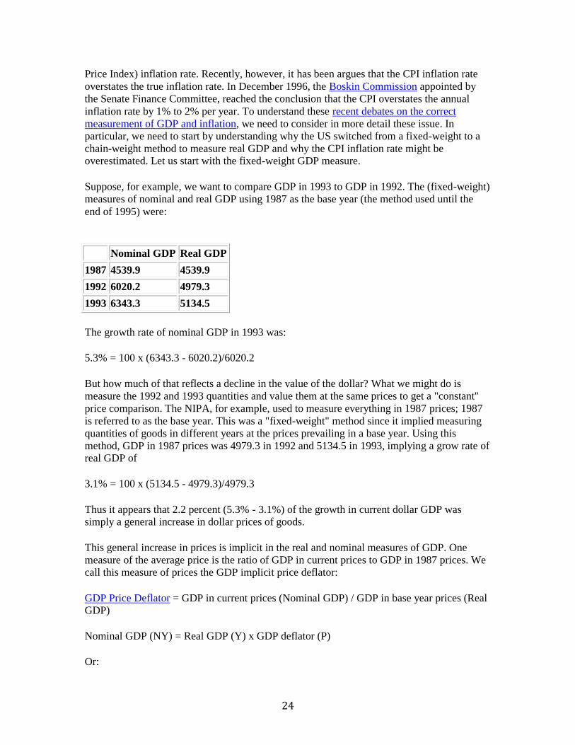
Suppose, for example, we want to compare GDP in 1993 to GDP in 1992. The (fixed-weight)

measures of nominal and real GDP using 1987 as the base year (the method used until the

end of 1995) were:

Nominal GDP Real GDP

1987 4539.9 4539.9

1992 6020.2 4979.3

1993 6343.3 5134.5

The growth rate of nominal GDP in 1993 was:

5.3% = 100 x (6343.3 - 6020.2)/6020.2

But how much of that reflects a decline in the value of the dollar? What we might do is

measure the 1992 and 1993 quantities and value them at the same prices to get a "constant''

price comparison. The NIPA, for example, used to measure everything in 1987 prices; 1987

is referred to as the base year. This was a "fixed-weight" method since it implied measuring

quantities of goods in different years at the prices prevailing in a base year. Using this

method, GDP in 1987 prices was 4979.3 in 1992 and 5134.5 in 1993, implying a grow rate of real GDP of

3.1% = 100 x (5134.5 - 4979.3)/4979.3

Thus it appears that 2.2 percent (5.3% - 3.1%) of the growth in current dollar GDP was simply a general increase in dollar prices of goods.

This general increase in prices is implicit in the real and nominal measures of GDP. One

measure of the average price is the ratio of GDP in current prices to GDP in 1987 prices. We call this measure of prices the GDP implicit price deflator:

GDP Price Deflator = GDP in current prices (Nominal GDP) / GDP in base year prices (Real GDP)

Nominal GDP (NY) = Real GDP (Y) x GDP deflator (P)

Or:

25

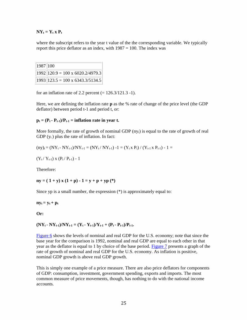
NYt = Yt x Pt

where the subscript refers to the year t value of the the corresponding variable. We typically

report this price deflator as an index, with 1987 = 100. The index was

1987 100

1992 120.9 = 100 x 6020.2/4979.3

1993 123.5 = 100 x 6343.3/5134.5

for an inflation rate of 2.2 percent (= 126.3/121.3 -1).

Here, we are defining the inflation rate p as the % rate of change of the price level (the GDP deflator) between period t-1 and period t, or:

pt = (Pt - Pt-1)/Pt-1 = inflation rate in year t.

More formally, the rate of growth of nominal GDP (nyt) is equal to the rate of growth of real GDP (yt ) plus the rate of inflation. In fact:

(ny)t = (NYt - NYt-1)/NYt-1 = (NYt / NYt-1) -1 = (Yt x Pt) / (Yt-1 x Pt-1) - 1 =

(Yt / Yt-1) x (Pt / Pt-1) - 1

Therefore:

ny = ( 1 + y) x (1 + p) - 1 = y + p + yp (*)

Since yp is a small number, the expression (*) is approximately equal to:

nyt = yt + pt

Or:

(NYt - NYt-1)/NYt-1 = (Yt - Yt-1)/Yt-1 + (Pt - Pt-1)/Pt-1.

Figure 6 shows the levels of nominal and real GDP for the U.S. economy; note that since the

base year for the comparison is 1992, nominal and real GDP are equal to each other in that

year as the deflator is equal to 1 by choice of the base period. Figure 7 presents a graph of the

rate of growth of nominal and real GDP for the U.S. economy. As inflation is positive, nominal GDP growth is above real GDP growth.

This is simply one example of a price measure. There are also price deflators for components

of GDP: consumption, investment, government spending, exports and imports. The most

common measure of price movements, though, has nothing to do with the national income accounts.

26

The Consumer Price Index measures the dollar price of a "fixed basket'' of goods rather than

the constant price of a changing basket of goods used to compute the "fixed-weight" GDP and its nominal price deflator.

The idea is to calculate the price of a constant list of goods at different points in time. Eg,

consider 5 gallons of gas, one haircut, 2 pounds of chicken, 3 bottles of soda, and so on. The

Bureau of Labor Statistics at the Department of Labor sends people to stores every month to

collect prices of the various goods, and then computes prices of various "baskets.'' The

Consumer Price Index (CPI) is the total price of all of these goods at different dates,

normalized to equal 100 at some date. Same idea, really, as the Dow Jones Industrial Average

or the S&P 500. The CPI takes its basket of goods from the typical spending patterns of an

American family.

The conceptual problem for both price indexes---the fixed-weight GDP deflator and the fixed

basket CPI deflator ---is that it's not clear how to measure the purchasing power of the dollar

when the dollar prices of different goods are changing at different rates. Conversely, it's not

clear how to combine quantities of different goods when their relative prices are changing. As usual, this is easier to see with an example.

Example (made-up numbers).

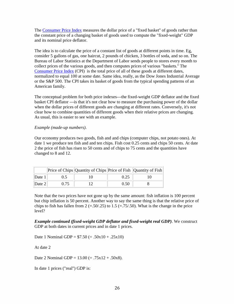
Our economy produces two goods, fish and and chips (computer chips, not potato ones). At

date 1 we produce ten fish and and ten chips. Fish cost 0.25 cents and chips 50 cents. At date

2 the price of fish has risen to 50 cents and of chips to 75 cents and the quantities have

changed to 8 and 12.

Price of Chips Quantity of Chips Price of Fish Quantity of Fish

Date 1 0.5 10 0.25 10

Date 2 0.75 12 0.50 8

Note that the two prices have not gone up by the same amount: fish inflation is 100 percent

but chip inflation is 50 percent. Another way to say the same thing is that the relative price of

chips to fish has fallen from 2 (=.50/.25) to 1.5 (=.75/.50). What is the change in the price level?

Example continued (fixed-weight GDP deflator and fixed-weight real GDP). We construct

GDP at both dates in current prices and in date 1 prices.

Date 1 Nominal GDP = $7.50 (= .50x10 + .25x10)

At date 2

Date 2 Nominal GDP = 13.00 (= .75x12 + .50x8).

In date 1 prices ("real'') GDP is:

27

Date 1 prices ("real'') GDP = 8.00 (= .50x12 + .25x8).

The GDP deflator (the ratio of current price GDP to GDP in base year prices, here date 1)

rises from 1.0 in the base year date 1 to 1.625 (= 13/8) at date 2, an inflation rate of 62.5 percent.

The the, real GDP growth measured with fixed weights is:

6.66% = 100 x (8-7.5)/7.5

In fact, since we know from (*) above that::

(1 + ny) = ( 1 + y) x (1 + p)

real growth y is:

y = [(1 + ny) / (1+p)] -1 = [(1 + 0.733)/(1 + 0.625)] -1 = 0.066

Consider now what happens to our measure of real GDP growth when we use a "fixed-

basket" based measure of inflation (the CPI index).

Example continued ("fixed-basket" CPI deflator and real GDP). The consumer price index

uses quantities in a base year to compute the costs of the same basket of goods at 2 different

dates. Let's say here that the basket of goods is 10 fish and 10 chips (the same composition as GDP). Then:

CPI at date 1 = 7.50 (= .50x10 + .25x10).

CPI at date 2 = 12.50 (= .75x10 + .50x10).

The implied CPI inflation rate is 66.6 (= 100 x (12.50-7.50)/7.50) percent.

Note the difference between the two indexes: the CPI uses date 1 quantities while the GDP

deflator uses date 2 quantities to compute the date 2 price index. (Check out the CPI

Calculation Machine at the Minneapolis Fed home page to get, say, the price of a cup of coffee in 1963).

Since nominal GDP growth is again 73.3% and the fixed-basket (CPI based) measure of

inflation is 66.6%, now the fixed basket measure of real GDP is 4% rather than the higher 6.66% obtained by using the fixed-weight method. In fact:

y = [(1 + ny) / (1+p)] -1 = [(1 + 0.733)/(1 + 0.666)] -1 = 0.04

How can we compute directly the real GDP growth if we use the CPI deflator ? Simple:

compute real GDP in the second period by taking period 2 as the base year (rather than period 1 as in the fixed-weight method). Then:

Period 2 Real GDP using date 2 as the base year: 13 = 0.75x12+0.5x8

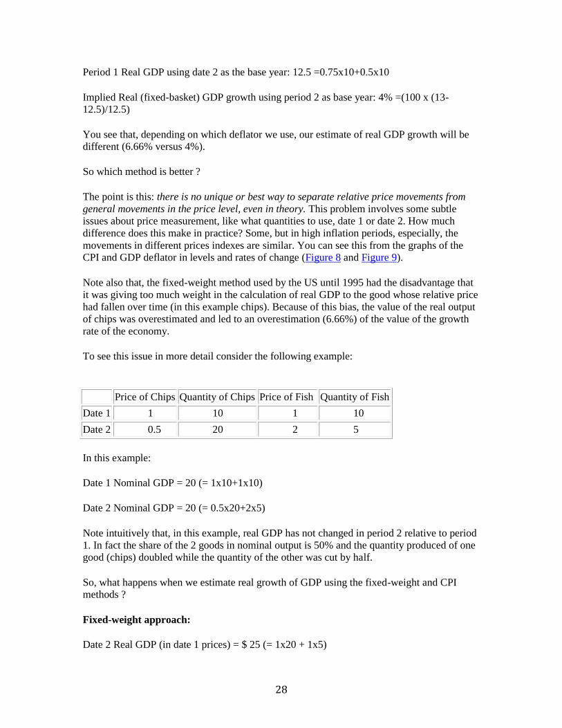
28

Period 1 Real GDP using date 2 as the base year: 12.5 =0.75x10+0.5x10

Implied Real (fixed-basket) GDP growth using period 2 as base year: 4% =(100 x (13-12.5)/12.5)

You see that, depending on which deflator we use, our estimate of real GDP growth will be different (6.66% versus 4%).

So which method is better ?

The point is this: there is no unique or best way to separate relative price movements from

general movements in the price level, even in theory. This problem involves some subtle

issues about price measurement, like what quantities to use, date 1 or date 2. How much

difference does this make in practice? Some, but in high inflation periods, especially, the

movements in different prices indexes are similar. You can see this from the graphs of the CPI and GDP deflator in levels and rates of change (Figure 8 and Figure 9).

Note also that, the fixed-weight method used by the US until 1995 had the disadvantage that

it was giving too much weight in the calculation of real GDP to the good whose relative price

had fallen over time (in this example chips). Because of this bias, the value of the real output

of chips was overestimated and led to an overestimation (6.66%) of the value of the growth

rate of the economy.

To see this issue in more detail consider the following example:

Price of Chips Quantity of Chips Price of Fish Quantity of Fish

Date 1 1 10 1 10

Date 2 0.5 20 2 5

In this example:

Date 1 Nominal GDP = 20 (= 1x10+1x10)

Date 2 Nominal GDP = 20 (= 0.5x20+2x5)

Note intuitively that, in this example, real GDP has not changed in period 2 relative to period

1. In fact the share of the 2 goods in nominal output is 50% and the quantity produced of one good (chips) doubled while the quantity of the other was cut by half.

So, what happens when we estimate real growth of GDP using the fixed-weight and CPI methods ?

Fixed-weight approach:

Date 2 Real GDP (in date 1 prices) = $ 25 (= 1x20 + 1x5)

29

Real 'fixed weight' GDP growth: 25% = (25/20)-1

GDP deflator inflation: -20%

Nominal GDP growth = 0 = (20-20/20) = (1 - 0.2)(1 + 0.25) -1

CPI (fixed basket) approach:

CPI inflation: 25% = [( 0.5x10 + 2x10) / 20] -1

Period 1 Real GDP using date 2 as the base year: 25

Period 2 Real GDP using date 2 as the base year: 20

Real GDP growth using date 2 as the base year: -20%

Nominal GDP growth = 0 = (20-20/20) = (1 + 0.25)(1 - 0.20) -1

The problem is that in fixed-weight approach, too much weight is given to production of the

good (chip) whose price has fallen over time. If we use a fixed-weight method, the output

level and growth rate is biased upward (we get an estimate of 25% real growth) because we are overestimating the value of the output of the good whose price has fallen.

It is like computing the real output of a PC computers in 1997 by taking the 1987 price of an

equivalent machine (approximately $6,000) as the base for valuing the real value added of a

PC that is priced only at $2,000 today. It does not make sense to value the quantity of

computers produced today at prices that were prevailing 10 years ago. So, the fixed-weight method led to an overestimation of the value added of the computer industry.

When the U.S. relied on the fixed-weight method, it was giving too much weight in the

calculation of real GDP to the good whose relative price had fallen over time (in this example

chips and in reality computers, semiconductors and other high tech sectors of the economy).

Because of this bias, the value of the real output of chips was overestimated and led to an

overestimation of the growth rate of the economy. This issue became serious over the 1980's

as the price of computers was falling in absolute and relative terms while the fixed-weight, by

using the high prices of computers prevailing in the base year, was leading to an overestimate

of the real GDP created by computers. In order to eliminate such a bias, the Department of

Commerce switched at the end of 1995 to a chain-weight method of measuring real GDP.

The chain weight method is a combination of the fixed-weight method and the fixed-basket

method. Real GDP is estimated twice, first using the previous year prices as the base (fixed-

weight) and the second time using the current year prices as the base and the previous year

quantities to compute real GDP in the previous year. Then, a (geometric) average of the two

is taken. Using this method:

Growth rate of chained GDP = [(1 + 0.25)(1- 0.2)-1]/2 = 0

i.e. the growth rate of chained GDP is equal to zero that is the sensible economic answer since real output in the example above had not changed in a substantial sense.

30

There are however several potential problems also with the chain-weight method:

1. Quality changes are not correctly measured (examples: computers, light) leading to under-estimate of the product of industries where such quality changes occur.

2. Major productivity growth in the service industries (ATM's, telecommunications, quality of health care) not measured by standard GDP measures.

First, an important issue in computing price indexes is how they deal with quality change and

new goods. One of the facts of life in growing economies is that the goods change: candy

bars change size, PCs have ever-increasing capabilities, and some goods simply didn't exist

in the base period. Candy bars are the easiest: we simply regard a five oz bar as half a ten oz

bar. But what about PCs? If a 286 sells for $2000 and a 386 for $4000, has there been

inflation or is the 386 machine twice as good as the 286? It's even more difficult if the

commodity has no counterpart in the base period. How do we include VCRs in the

calculation when they didn't exist, for all practical purposes, prior to the 1980s? For this

reason, some people think that price indexes and real GDP do not adequately reflect quality

improvements---that real GDP is growing faster than we think because quality is constantly improving. That's especially true now of new high-tech capital goods.

Second, related issues show up in services. Many authors (including the Fed Chairman Alan

Greenspan) have argued that major productivity growth in the service industries are not

measured by standard GDP measures. Moreover, there are other subtle measurement issues:

if the price of one hour of a lawyer's time goes up, does this represent an improvement in

quality or just a rise in the price?

Critics of the switch from fixed-weights to chain-weights have argued that, while the fixed-

weight method overestimated the contribution of computers to real GDP, the chain-weight

method fixes one problem but does nothing to address the two issues above; that, on net,

leads to an underestimation of real GDP. So the new measure might overall tend to underestimate GDP and its growth rate.

At the same time, a number of authors have argued that the use of the CPI inflation rate also

tends to overestimate the true level of inflation rate in the US economy because of a number

of biases. In December 1996, the Boskin Commission appointed by the Senate Finance

Committee, reached the conclusion that the CPI overstates the true inflation rate by 1% to 2%

per year. Note that, if inflation is overestimated, then our measure of real GDP growth is

underestimated as well as more of the growth of nominal GDP is imputed to an increase in

prices than to an increase in quantities produced. A wide debate on the CPI has followed the

publication of the Boskin Commission recommendations. Fed Chairman Alan Greenspan has

expressed his views on this debate in a testimony in Congress in January 1997 and a recent speech in November 1997.

For more discussion on these issues see the home page on the debate on whether output and CPI inflation are mismeasured.

Summary

31

1. GDP measures the total value of production at market prices, the sum of value-added

by every production unit in the economy.

2. Identities.

o Output (GDP) = Income (payments to labor and capital, gross of

depreciation).

o GDP = C + I + G + NX .

o GNP = GDP + i NFA = C + I + G + (NX + i NFA) .

o GNP = C + I + G + CA .

o S = I + CA .

3. Price indexes measure the purchasing power of money. Issues: relative price vs

general price level movements, quality change and new goods.

4. Bottom line: economic indicators clearly contain useful information, but like

accounting statements they must be interpreted with care. [Data are like sausages: if

you like them, you shouldn't think too much about what goes into them.]

Further Readings

For a wealth of WEB-based data and analysis of the U.S. and world economy, check out the

WEB sites listed in the our home pages on Macro Data and Analysis Links and Business

Cycle Indicators.

On paper, there are two good (by which I mean informative and readable) books on the uses,

sources, and meaning of economic data: Norman Frumkin's Guide to Economic Indicators

(Armonk: Sharpe, 1994, 2nd edition) or Tracking America's Economy (Armonk: Sharpe,

1992). Not needed for this course, but if you ever have to look something up it's a good place

to start. A slightly more technical introduction to macroeconomic data is available from the

Richmond Fed: Macroeconomic Data: A User's Guide, edited by Roy Webb. Both of these

cover the US, but in many cases the methods are similar to those used in other countries

(especially for national income and product accounts, for which there is a United Nations standard).

Further Web Links and Readings

The course home page on the controversy about whether output and CPI inflation are

mismeasured is a useful source of materials on the chain-weight measure of GDP, on the

results of the Boskin Commission and the debate on these results. The debates on the chain-

weight system of measuring GDP and the biases in measuring the inflation rate are also

related to the question of whether we are correctly measuring productivity growth and

whether there has been a resurgence of productivity growth in the 1990s after the dismal

productivity experience in the 1973-1990 period (see also Chapter 4). On this debate and the

related issue of the productivity slowdown see the homepages on the controversies

Productivity Growth, Its Slowdown in the 1973-90 period and its resurgence in the 1990s:

Truth or a Statistical Fluke? and the New Economy.

Table 1

Saving and Investment Rates for Developed Countries.

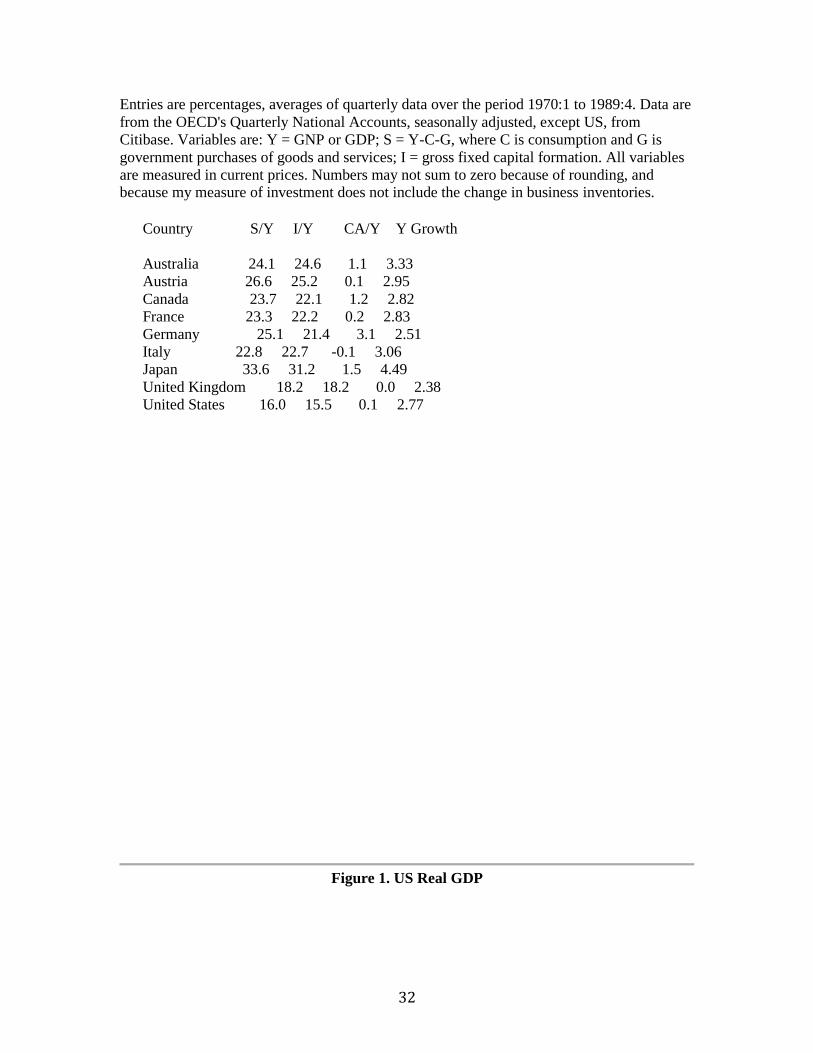
32

Entries are percentages, averages of quarterly data over the period 1970:1 to 1989:4. Data are

from the OECD's Quarterly National Accounts, seasonally adjusted, except US, from

Citibase. Variables are: Y = GNP or GDP; S = Y-C-G, where C is consumption and G is

government purchases of goods and services; I = gross fixed capital formation. All variables

are measured in current prices. Numbers may not sum to zero because of rounding, and because my measure of investment does not include the change in business inventories.

Country S/Y I/Y CA/Y Y Growth

Australia 24.1 24.6 1.1 3.33

Austria 26.6 25.2 0.1 2.95

Canada 23.7 22.1 1.2 2.82

France 23.3 22.2 0.2 2.83

Germany 25.1 21.4 3.1 2.51

Italy 22.8 22.7 -0.1 3.06

Japan 33.6 31.2 1.5 4.49

United Kingdom 18.2 18.2 0.0 2.38

United States 16.0 15.5 0.1 2.77

Figure 1. US Real GDP

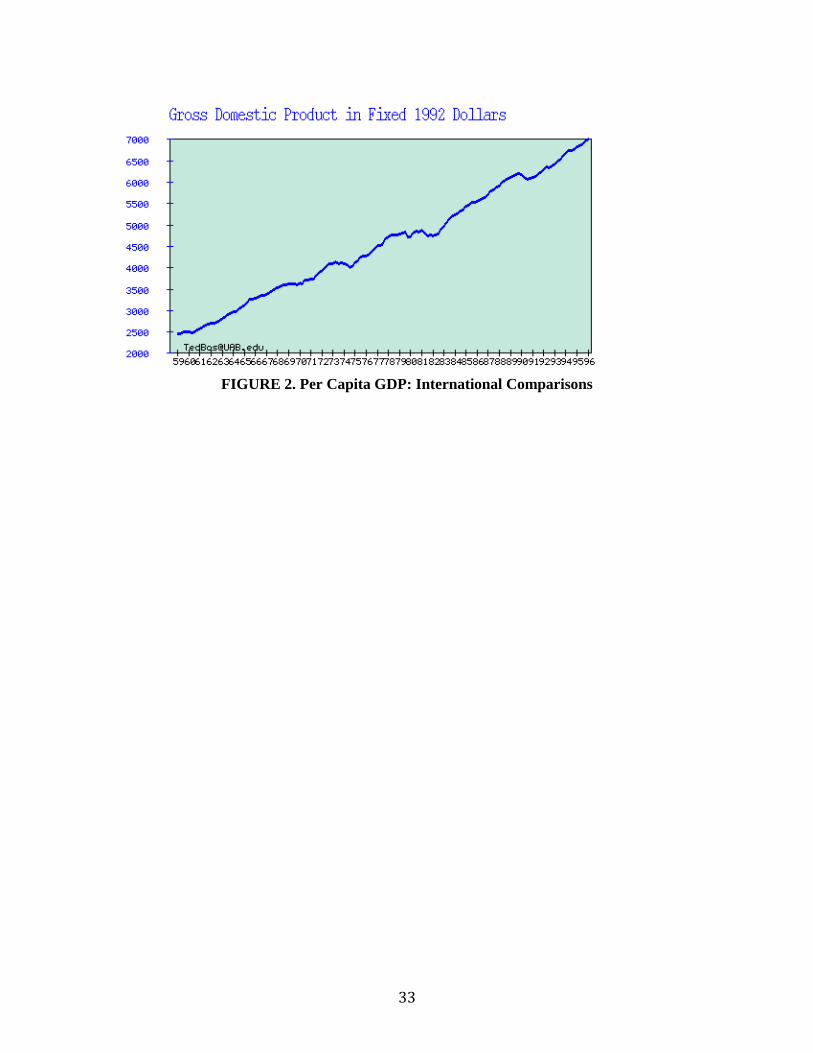
33

FIGURE 2. Per Capita GDP: International Comparisons

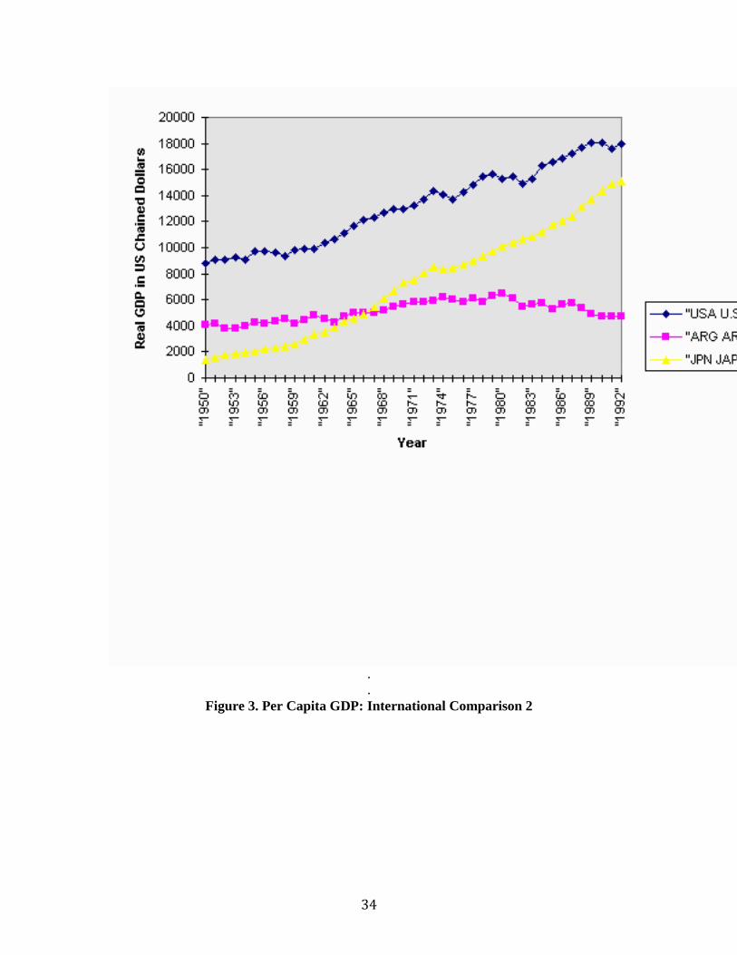
34

.

.

Figure 3. Per Capita GDP: International Comparison 2

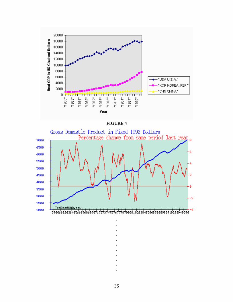
35

FIGURE 4

.

.

.

.

.

.

.

.

.

.

.

36

.

FIGURE 4'

Figure 5. GNP Growth in Germany and Japan

.

Figure 6

Nominal and Real GDP

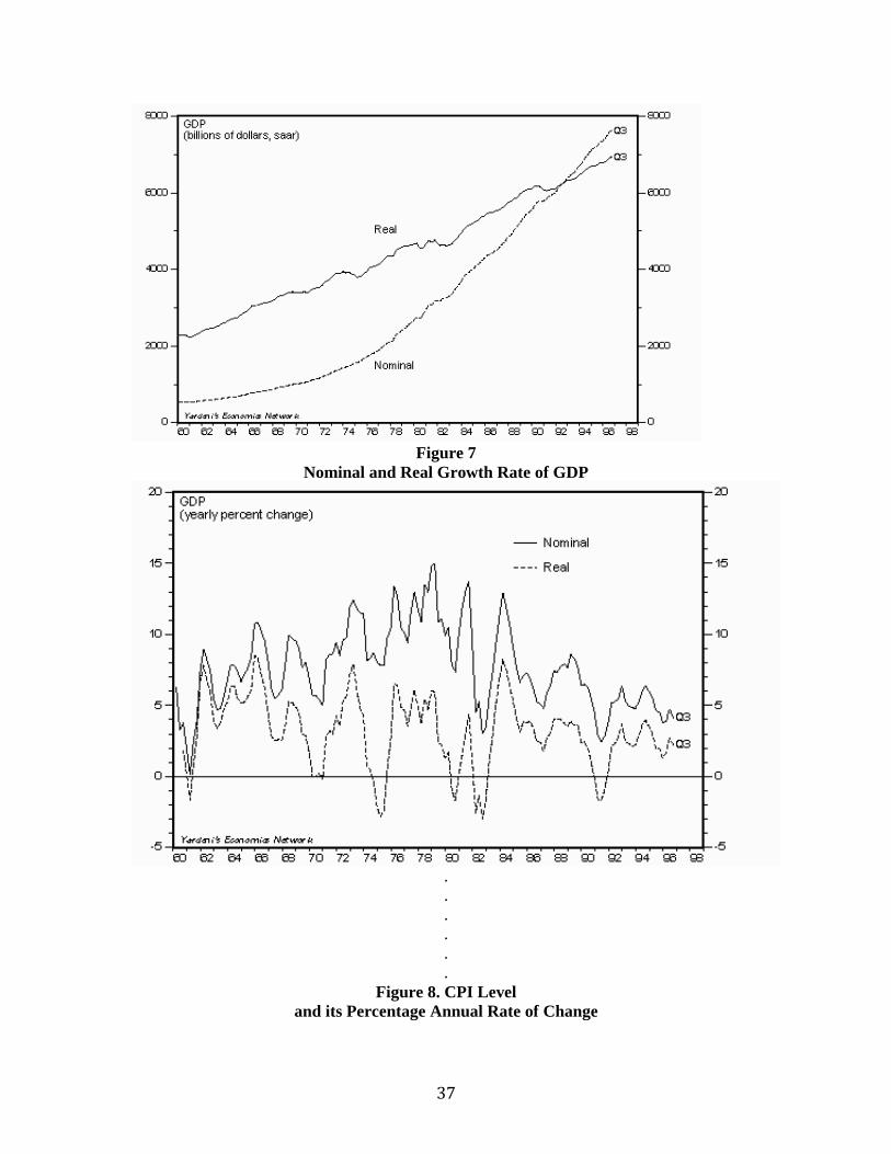
37

Figure 7

Nominal and Real Growth Rate of GDP

.

.

.

.

.

.

Figure 8. CPI Level

and its Percentage Annual Rate of Change

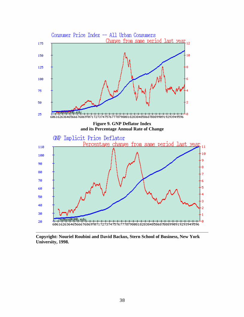
38

Figure 9. GNP Deflator Index

and its Percentage Annual Rate of Change

Copyright: Nouriel Roubini and David Backus, Stern School of Business, New York

University, 1998.

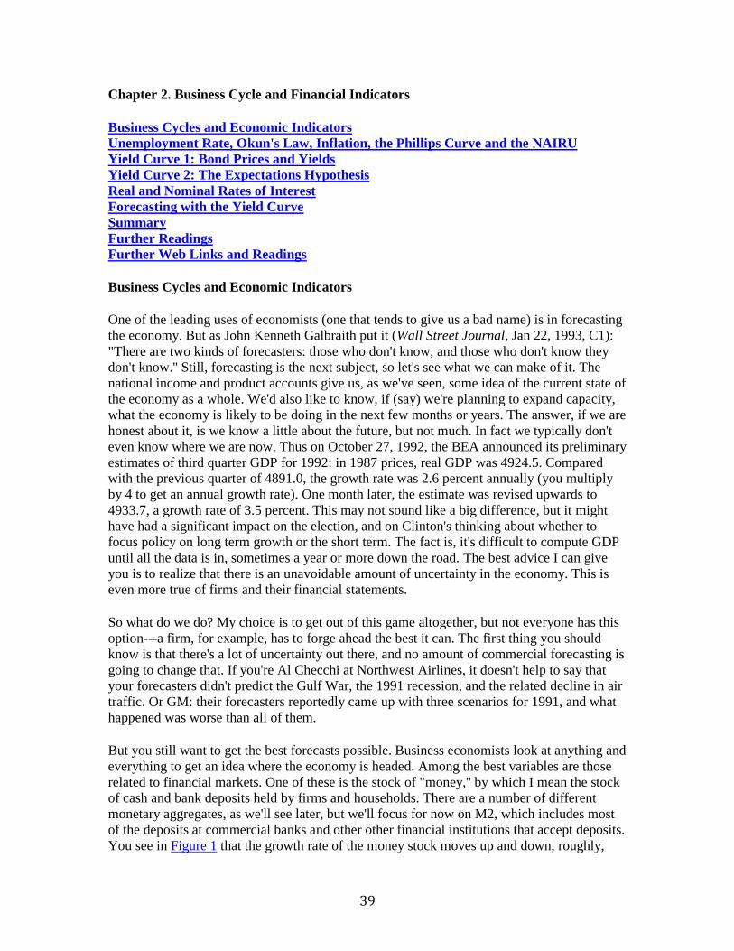
39

Chapter 2. Business Cycle and Financial Indicators

Business Cycles and Economic Indicators

Unemployment Rate, Okun's Law, Inflation, the Phillips Curve and the NAIRU

Yield Curve 1: Bond Prices and Yields

Yield Curve 2: The Expectations Hypothesis

Real and Nominal Rates of Interest

Forecasting with the Yield Curve

Summary

Further Readings

Further Web Links and Readings

Business Cycles and Economic Indicators

One of the leading uses of economists (one that tends to give us a bad name) is in forecasting

the economy. But as John Kenneth Galbraith put it (Wall Street Journal, Jan 22, 1993, C1):

"There are two kinds of forecasters: those who don't know, and those who don't know they

don't know.'' Still, forecasting is the next subject, so let's see what we can make of it. The

national income and product accounts give us, as we've seen, some idea of the current state of

the economy as a whole. We'd also like to know, if (say) we're planning to expand capacity,

what the economy is likely to be doing in the next few months or years. The answer, if we are

honest about it, is we know a little about the future, but not much. In fact we typically don't

even know where we are now. Thus on October 27, 1992, the BEA announced its preliminary

estimates of third quarter GDP for 1992: in 1987 prices, real GDP was 4924.5. Compared

with the previous quarter of 4891.0, the growth rate was 2.6 percent annually (you multiply

by 4 to get an annual growth rate). One month later, the estimate was revised upwards to

4933.7, a growth rate of 3.5 percent. This may not sound like a big difference, but it might

have had a significant impact on the election, and on Clinton's thinking about whether to

focus policy on long term growth or the short term. The fact is, it's difficult to compute GDP

until all the data is in, sometimes a year or more down the road. The best advice I can give

you is to realize that there is an unavoidable amount of uncertainty in the economy. This is

even more true of firms and their financial statements.

So what do we do? My choice is to get out of this game altogether, but not everyone has this

option---a firm, for example, has to forge ahead the best it can. The first thing you should

know is that there's a lot of uncertainty out there, and no amount of commercial forecasting is

going to change that. If you're Al Checchi at Northwest Airlines, it doesn't help to say that

your forecasters didn't predict the Gulf War, the 1991 recession, and the related decline in air

traffic. Or GM: their forecasters reportedly came up with three scenarios for 1991, and what

happened was worse than all of them.

But you still want to get the best forecasts possible. Business economists look at anything and

everything to get an idea where the economy is headed. Among the best variables are those

related to financial markets. One of these is the stock of "money,'' by which I mean the stock

of cash and bank deposits held by firms and households. There are a number of different

monetary aggregates, as we'll see later, but we'll focus for now on M2, which includes most

of the deposits at commercial banks and other other financial institutions that accept deposits.

You see in Figure 1 that the growth rate of the money stock moves up and down, roughly,

40

with the growth rate of GDP. In this sense it is a good indicator of the state of the economy.

And since money stock measures are generally made available more quickly than GDP, it tells us something about the current state of the economy as well.

Even better indicators are financial prices and yields, which have the additional advantage of

being available immediately. As you might expect if you've ever taken a finance course, asset

prices tend to incorporate "the market's'' best guess of future events and, by and large, they

are as good predictors of the economy as we have. Maybe the best of these is the stock

market. In Figure 2 I've plotted the annual growth rate of real GDP with the annual growth

rate of the S&P 500 composite stock index. What you might expect is that the stock market

anticipates movements in the economy: in recessions profits and earnings are down so stock

prices should fall as soon as a recession is anticipated by the market. That's pretty much what

you see. In the figure we see that every postwar downturn in the economy has been at least

matched, if not anticipated, by the stock market. The problem is that there have been several

downturns in the stock market that didn't turn into recessions---so-called false signals. A

classic case is the October 1987 crash, which was followed by several years of continued

growth. As we say in the trade, the stock market has predicted twelve of the last eight recessions.

Other useful financial variables are yield spreads, especially the long-short spread (the

difference between yields on long- and short-term government bonds) and the junk bond

spread (the difference between yields on high- and low-grade bonds). Both of these have

been useful in predicting downturns in the economy. Recent work by Stock and Watson for

the NBER suggests that stock prices and yield spreads contain almost all the usable statistical information about the future of the economy.

Financial variables and some others are combined in the official index of leading indicators,

which is constructed every month by the Conference Board and reported in the Wall Street

Journal and other business publications. The current index of leading indicators (it changes from time to time) combines the following series:

Leading Indicators

1. Hours of production workers in manufacturing

5. New claims for unemployment insurance

8. Value of new orders for consumer goods

19. S&P 500 Composite Stock Index

20. New orders for plant and equipment

29. Building permits for private houses

32. Fraction of companies reporting slower deliveries

83. Index of consumer confidence

41

99. Change in commodity prices

106. Money growth rate (M2)

(The numbers are labels assigned in Business Conditions Digest, a Commerce Department

publication on the state of the economy.) We see in Figure 3 that the index is closely related

to the cycle, but only leads it by a month or two (which is hard to see in the quarterly data

that I've graphed). Nevertheless, this is useful, since we don't know yet what GDP was last

month. A related index of coincident indicators (Figure 4) does not lead the cycle, but has a stronger correlation with it. Its components are

Coincident Indicators

41. Nonagricultural employment

47. Index of industrial production

51. Personal income

57. Manufacturing and trade sales

Both of these indexes combine economic indicators to give us a clearer picture of current and, to a limited extent, future economic conditions.

What are the business cycle properties of other macroeconomic variables ? The attached

figures of various macro series presented at the end of the chapter can be interpreted as

follows. Industrial production is pro-cyclical and coincident; both consumption and

investment are pro-cyclical with investment more sensitive than consumption to the business

cycle, as durable goods are a larger fraction of investment than of consumption; capacity

utilization is procyclical; employment is pro-cyclical and coincident; the unemployment rate

is countercyclical; the inflation rate is pro-cyclical and lags the business cycle (it tends to

build up during an expansion and fall after the cyclical peak); the short-term nominal interest

rate is pro-cyclical and lagging; corporate profits are very pro-cyclical as they tend to increase during booms and strongly fall during recessions.

More information on business cycle is provided in the course homepage on Business Cycle Indicators and the Hyptertext Glossary of Business Cycle Indicators.

If we use these data, how well do we do in forecasting the future? The short answer is that

there's a lot of uncertainty in the economy, and no amount of economic or statistical

sophistication is going to change that. Let me try to make this specific (at the risk of being a

little technical). Using time series statistics (which I'll presume you remember from your

Data Analysis course) you might estimate a linear regression of the form,

gtk = a + b xt ,

where gtk is the annualized growth rate between time t ("now'') and time t+k ("later''), with

time measured in quarters. The variable x is whatever you use to predict g . If we do all this,

42

we can use the estimated equation to forecast future GDP and get a quantitative measure of

the amount of uncertainty in the economy as a whole. That is, we plug in the current value of

the leading indicators for x and the latest estimate of GDP, and use the equation to tell us

what GDP in k quarters is expected to be, relative to GDP now.

We find, of course, that our predictions are invariably wrong, sometimes by a little,

sometimes a lot. A measure of how well we do is the standard deviation of the forecast error,

the difference between what we predicted and what actually happened. To make this

concrete, I used for x the spread between the ten-year treasury yield and the 6-month tbill

yield. The parameters a and b of the regression line were then estimated by least squares. The

estimates of b are invariably positive, indicating that upward sloping yield curves (see the

next section) indicate high growth, downward sloping yield curves the reverse. The overall performance of this procedure is summarized by the statistics:

Forecast Horizon (k) Std Deviation of Forecast Error R2 1

quarter 0.9% 0.11 4

quarters 2.1% 0.30 8

quarters 3.2% 0.25

The technical aspects were discussed in your Data Analysis course, but to understand what

the numbers mean let me run through the predictions for k=4. We find that for predictions of

the growth rate of GDP between now and a year from now (k=4) that only 30 percent of the

typical yearly variation (the variance) is predictable. The other 70 percent is unpredictable (at

least by this method). We also see that the standard deviation of the forecast error is 2.1

percent: that is, we expect our prediction to be within 2.1 percent, in either direction, of what

actually occurs about 70 percent of the time, which is a pretty wide band (Think of telling

your boss: sales will either grow 3 percent this year or fall 1 percent.) This is a simple

procedure, you might be able to do better. But it's unlikely that you'll consistently do a lot

better. (If you do, you should go into business.) It gives us a concrete measure of how much

uncertainty is out there in the economy as a whole, and indicates that there's a lot going on

that's unpredictable. For individual firms it's worse, since lots of things affect individual firms

that don't show up in the aggregate.

Perhaps the best lesson you can take from this is that the future is, to a large extent,

unpredictable. It's misleading, and probably dangerous, to assume otherwise, no matter what

you pay your economists. One of the things you probably want to do in business is learn to

deal with uncertainty. You might do this by making contingency plans, so you'll be prepared

when something unexpected occurs, by following flexible manufacturing methods so that you

can adapt your product quickly if the market changes, by adopting a financial strategy that

hedges you against (say) adverse movements in interest rates or currencies, and so on. That's

not the topic of this course, but it may help to put some of what you learn in other courses in perspective.

Unemployment Rate, Okun's Law, Inflation, the Phillips Curve and the NAIRU.

We consider now a number of other important business cycle concepts.

The labor force is the sum of employed and unemployed:

43

Labor Force = Number of Employed + Number of Unemployed

L = N + UN

The Unemployment Rate is defined as the percentage of the labor force that is unemployed:

U = (Unemployment Rate) = 100 (Number of Unemployed) / (Labor Force)

U = 100 (UN / L)

Okun's Law: The relation between the growth rate of GDP and changes in the

unemployment rate.

Since employed workers contribute to the production of goods while unemployed workers do

not, increases in the unemployment rate should be associated with decreases in the growth

rate of GDP. This negative relation between changes in the unemployment rate and GDP growth is called Okun's Law. Based on U.S. data we can write such a law as:

Growth rate of GDP = (Natural Growth Rate of GDP) - 2 (Change in the Unemployment Rate)

(Yt - Yt-1)/Yt-1 = 2.5% - 2 (Ut - Ut-1)

where the subscript t refers to the period under consideration. If the data are on a yearly

frequency, the expression above relates the growth rate of the GDP between year t and year t-

1 to the change in the unemployment rate between year t and year t-1. The law says that if the

unemployment rate stays the same relative to the previous year, real GDP in a year grows by

around 2.5% per year; this is the normal long-run growth rate of the economy (or natural

rate of growth) due to population growth, capital accumulation and technological progress. In

the example above this natural rate of growth is assumed to be 2.5%. For the US economy

such a natural rate of growth is currently believed to be in the 2.5% to 3.0% range. More on this issue will be discussed below.

Another relation to consider is the Phillips Curve or the relation between the inflation rate

and the unemployment rate: this relation suggests that when the unemployment rate is low

inflation tends to increase while when the unemployment rate is high inflation tends to decrease. More specifically, this curve posits that the inflation rate depends on three factors:

1. The expected inflation rate (pte) in year t.

2. The deviation of the unemployment rate (Ut ) in year t from the natural unemployment rate (Ut

n).

3. A supply shock (x) (for example, an oil price shock).

So:

pt = pte - a (Ut - Ut

n) + x

44

where the inflation rate (pt) is the yearly rate of change of the price level (the % rate of

change of the CPI or GDP deflator between year t and year t-1):

pt = (Pt - Pt-1 )/ Pt-1

(Utn) is the natural rate of unemployment determined by structural long-term factors that

determine how many workers will be unemployed even the the economy is running at full capacity and close to its long-run potential growth rate.

If, as appears to be the case in the United States today, the expected rate of inflation (pte) is

well approximated by last year's inflation rate (t-1), the relation becomes:

pt = pt-1 - a (Ut - Utn) + x

This relation links the the difference between the actual rate of unemployment and the natural

rate of unemployment to the change in inflation. When the actual unemployment rate exceeds

its natural rate, inflation decreases; when the actual unemployment rate is less than the

natural rate, inflation increases. So, the natural rate of unemployment can be seen as the rate

of unemployment required to keep inflation constant. This is why the natural rate of

unemployment is also called the Non-Accelerating Inflation Rate of Unemployment or

NAIRU. Note that the natural rate and its changes over time are hard to measure since we

observe only the actual unemployment rate. There is currently a debate in the U.S. about

what is the natural rate or the NAIRU. Usually, the level and the broad changes in the natural

rate can be measured by comparing average unemployment rates in various decades. The

average unemployment rate was 4.4% in the 1960s, 6.2% in the 1970s, 7.2% in the 1980s and

6.2% in the 1990s. If we believe that the natural rate is equal to the average unemployment

rate in the decade, the current (November 1996) 5.4% unemployment rate is below the

natural rate of 6.2%. Most mainstream economists believe that the natural rate is now closer

to 5.5% as the actual unemployment rate was high during the 1990-91 recession. Even if the

natural rate is 5.5%, we get a puzzle: according to the NAIRU curve, the inflation rate should

have been increasing since the late part of 1995 when the unemployment rate fell below the

5.5% level. Instead there is no evidence that the inflation rate is accelerating these days. What can explain this contradiction ? There are very different alternative explanations:

1. According to some, there are structural changes in the economy that have led to a reduction of the NAIRU to a level closer to 5% or even below that.

2. According to others, we are already below the natural rate now and inflation will start to

increase soon. According to this interpretation we have not seen the increase in inflation yet

only because there were a series of favorable supply shocks (x) that have maintained the

inflation rate low so far. But inflation will start to increase soon unless the economy growth rate slows down and the unemployment goes back above the 5.5% level.

For more on this current policy debate see the course homepages on the NAIRU controversy and the New Economy.

Yield Curve 1: Bond Prices and Yields

45

The yield curve for US treasury securities is published every day in the Wall Street Journal .

And lots of other places, too: for example, the Department of Commerce home page gives

you daily data for the Treasury yield curve. Nice charts of the yield curve (and expected

future interest rates) can be found in the 'Monetary Policy' section and 'Interest Rates' section

of the "Economic Trends" by the Research Department at Federal Reserve Bank of

Cleveland, a monthly source of analysis of US macroeconomic conditions.

The yield curve tells you at a glance how short- and long-term interest rates differ and also

provides, as we've seen, an indicator of economic growth; see Figure 5 for some recent charts

of the yield curve. We'll come back to that shortly, but first we need to go through the arithmetic of treasury prices and yields.

The first lesson is that price is fundamental. Once you know the price of a bond, you can

easily compute its yield. The yield---or more completely, the yield to maturity---is just a

convenient short-hand for expressing the price as a rate of return: the average compounded

return on a security if you hold it until it matures. Equivalently, prices are present values,

using yields as discount rates. The details reflect a combination of the application of the

theory of present values and the conventions of the treasury market (or whatever market

you're looking at).

We'll start with a relatively simple problem: yields on bonds with no coupons. These are

generally referred to as "strips'' or "zeros'' (for "zero-coupon''), with prices reported under

"Treasury Bonds, Notes & Bills'' in Section C of the Journal. By convention the principal or

face value of the bond is $100. If we label the price of a one-year bond of this type p1 , then the price plus interest at rate i equals the principal; that is,

100 = p1(1 + i).

Equivalently, we say that the price is the present discounted value of the principal:

p1 = 100/(1 + i).

We refer to i as the short rate since it's the yield on a short-term bond, but it's also the yield-

to-maturity on a one-period bond, which we might label y1 ( y for yield). Mathematically

what we've shown is that when you know the price, you can solve one of these equations to

find the yield. [For some weekly updated charts (going back to 1995) of short-term and long-

term US interest rates look at the Interest Rate Charts in the home page of the Minneapolis

Fed]. Longer sample series that are updated every month can be charted using the Economic

Chart Dispenser .

Longer bonds work pretty much the same way. For a two-year bond (again, with no coupons)

we can think of the yield as the compounded return over two periods, 100 = p2(1 + y2)2 ,

which gives us the present value relation

p2 = 100/(1 + y2)2.

Similarly, for an n-year bond the formula would be

46

pn = 100/(1 + yn)n ,

where pn and yn are the price and yield of an n-year bond. As with the one-year bond, you can

compute the yield from the price. A similar method is used for treasury securities and

corporate bonds in the US, but by convention yields in these markets are compounded every six months rather than once a year, a complication we will ignore.

Examples. Let the prices of zero-coupon bonds be

Maturity in Years Price 1 94.24 2 87.70 3 81.22

4 75.16 5 69.66

The yields are, resp, 6.11 percent per year, 6.78, 7.18, 7.40, and 7.50. This gives us five

points on a yield curve.

With coupons, bond pricing gets a little more complicated, but the idea is the same: the price

is the present value of cash flows, discounted at a rate we call the yield. In this case the cash

flows include coupons as well as principal. Given the price, we solve this relation for the

yield. Take, for example, a 6% 3-year bond, with a coupon of 6 dollars every twelve months

for every 100 dollars of face value. (Again: US treasury and corporate bonds are slightly

different, with coupon payments every six months.) Then the yield is the discount rate that

equates the price with the sum of the present discounted values of coupons plus principal. Mathematically (this may be one of those cases where the math is simpler than the words),

p = 6/(1+y) + 6/(1+y)2 + 106/(1+y)3 .

That is, we get 3 coupons and one principal payment, discounted accordingly. By way of

example, if the price is 97.01 the yield is 7.14 percent (which you'll note is a little smaller than the three-year yield on a zero, 7.18).

This solution for the yield y involves some nasty algebra once we add coupons, but is easily

accomplished on a spreadsheet. Probably the most straightforward way to do this is to define

a formula relating the price to the yield y, then choose different values for y until one gives

you the price quoted in the market. Another way, which runs the risk of confusing you, is to

use a built-in function on your calculator or spreadsheet. Warning: these functions differ in

subtle ways. I suggest you test yours with this or other example before relying on the answers it gives.

Yield Curve 2: The Expectations Hypothesis

Now that we have some idea what the yield curve is, we can try to interpret its shape. The

idea I want to get across is that the yield curve tells us about future short term interest rates.

If the yield curve is downward sloping, for example, this generally means that the market

anticipates a decline in short term interest rates in the future. The theory to this effect is

called the expectations hypothesis, since it's based on the idea that long rates incorporate

market expectations of future short rates.

Forward rates. To make this concrete, we need to use (unfortunately) more complicated

notation. Let us say, to be specific, that we are interested in the yields on one- and two-period

47

zero-coupon bonds, with periods of one year. Then we know, for example, that the price of a

two-year bond satisfies

100 = p2 (1+ y2)2 = p2 (1 + y2)(1 + y2).

One interpretation of this relation is that the owner of the bond gets a rate of return y2 in the

first period and y2 again in the second, compounded. The subscript 2 on y means that this is the yield on a two-period bond.

A second interpretation allows the two periods to have different rates of return, since there's

no particular reason periods must be alike. In the first period the return is simply the short

rate in the first period, which I'll label i1, the yield y1 on a one-period bond. The added

subscript 1 in i1 means that we're talking about the first period, something we took for

granted earlier. The second period of the bond, considered on its own, is what we call a

forward contract: we contract now for an investment made one period from now and lasting

until the end of the second period. Thus, a two-period bond is a combination of a one-period

bond and a one-period-ahead forward contract. By this interpretation the 100 principal is, again, the purchase price plus two periods of interest:

100 = p2 (1+ i1)(1+ f2),

where f2 is the return on a forward contract in the second period. We can combine the two relations in the equation,

(1 + y2)2 = (1+ i1)(1+ f2),

which shows us how the yield curve defines the forward rate.

Although it's not necessary for our purposes, we can extend this use of forward contracts to

as many periods as we like. Eg, a four-period bond is a combination of a one-period bond and

three successive forward contracts. Thus we can express the yield in terms of the rates on these contracts:

(1+ y4)4 = (1+ i1)(1 + f2)(1 + f3)(1 + f4).

From the prices or yields of bonds with maturities 1 through 4, we can compute the implicit

forward rates. Alternatively, we could compute forward rates directly from bond prices: 1 +

fn = pn / pn+1. These forward rates define a forward rate curve, analogous to the yield curve.

This curve is not the same as the yield curve, but if the forward rate curve is upward

(downward) sloping, then so is the yield curve. They simply report the same information in

slightly different ways. The reason for all this is to try to make sense of the maturity structure of bond prices, and this is a little more direct if we use forward rates rather than yields.

Example (continued). Consider the bond prices and yields from the last section. You might

verify that the forward rates are

Maturity Price Yield Forward Rate

48

1 94.24 6.11 (6.11)

2 87.70 6.78 7.45

3 81.22 7.18 7.98

4 75.16 7.40 8.06

5 69.66 7.50 7.90

Expectations hypothesis. Now consider what investors might demand of forward rates. An

investor with a two-period time horizon has (at least) two choices. She could buy a two-

period bond, thus getting (according to our second interpretation) i1 in the first period and f2

in the second. Alternatively, she could "roll over'' a one-period bond, getting (again) i1 the

first period and the short rate i2 in the second. The notation i2 here means the short rate in the

second period. These two possibilities can be pictured like this:

.

.

.

Rollover Strategy i1 i2 X--------------X------------

X i1 f2 Long Bond Strategy

If i2 were known with complete certainty, then we would expect the market to drive the

forward rate f2 and the future short rate i2 together: if, say, the future short rate were higher,

then no one would buy the long bond. In an uncertain world, a similar guess might lead us to

guess that the forward rate is the market's best guess of the future short rate, with some

adjustment for risk. Mathematically, we could write

f2 = E( i2 ) + risk premium,

where E(.) means the expectation of what's in parentheses and the risk premium is the

(presumed constant) adjustment for risk. With more distant forward rates we might say, for similar reasons,

fn = E( in ) + risk premium,

with the understanding that the risk premium can differ across maturities n .

In words: the expectations hypothesis is that forward rates are forecasts of future short-term

interest rates --- plus a risk premium. Thus we can read the forward rate curve as a forecast of

what short rates will do in the future. For example, if forward rates are below the current

short rate, we interpret this as saying that bond buyers expect the short rate to decline in the

future. And if forward rates exceed the current short rate by more than the risk premium, then

they expect the short rate to increase. The trick is estimating the risk premium. There are as

many ways to do this as there are finance professors, but a relatively simple method is to use

the average difference between the short rate and the n-period forward rate as an estimate of

its risk premium. Thus we see in Table 1 that the average short rate (the 12-month yield in

the table) over the more recent 1982-1991 period has been 8.563 percent per year. The

average 2-year forward rate f2 has been a little higher: 9.472 (I read this from the 24-month

forward rate in Panel B of the same table). The difference of 0.909 I use as an estimate of the

risk premium. Similarly, the risk premium for the 3-year forward rate is, similarly, the

difference between 9.923 and 8.563, or 1.360 percent. If we continue to fill out the table this way we get

49

Maturity Price Yield Forward Rate Risk Premium Future Short Rate

1 94.24 6.11 (6.11) 0.00 (6.11)

2 87.70 6.78 7.45 0.91 6.54

3 81.22 7.18 7.98 1.36 6.62

4 75.16 7.40 8.06 1.27 6.79

5 69.66 7.50 7.90 1.62 6.28

We see, roughly, that the risk premium increases with maturity. The exception at 4 years is as

likely to be noise in the data as anything else.

Given estimates of the risk premiums, we simply subtract to get an estimate of the market's

forecast of future short rates. Thus the forward rate of f2 = 7.45 indicates, given an estimated

risk premium of 0.91, a forecast of 6.54 for the short rate one year from now, an increase of 43 basis points (0.43 percent) relative to the short rate reported in the table.

In short, the expectations hypothesis tells us we can read the yield curve, and the closely

related forward rate curve, as telling us the market's prediction of future short rates. This

theory is the starting point for more advanced bond pricing theories, some of which you can

learn about in the Debt Instruments course. More advanced theories generally go on to relate

the risk premium to the risks involved in buying and selling bonds of different maturities.

Real and Nominal Rates of Interest

Yields, as we have constructed them, have units of dollars: they tell us how many dollars we

get in (say) one year in return for a given investment of dollars now. For example, if a 12-

month treasury bill has a price of 96 dollars, its yield i is the solution to

96 (1+i) = 100 ,

implying an interest rate of about 4 percent. Thus each dollar invested today gives us about

1.04 dollars in 12 months. Since i is measured in dollars, we refer to it as the nominal or

money rate of interest. For many purposes, though, we want to know not only the dollar

yield, but how much the 1.04 will buy when we get it. Given an inflation rate now of about 3

percent per year, we can expect that about 3 percent of the 4 percent rate of interest will be

eaten up by inflation. The investment only gains us about 1 percent per year in terms of what

it will buy.

This inflation adjustment defines a real rate of interest r : the difference between the

nominal rate of interest i and the expected rate of inflation, which I label pe . As an equation,

we might express this

r = i - pe .

A more complex version of this follows, but can easily be skipped if you think this makes sense as it stands.

The idea behind this expression is that interest rates have units, and in principle we can

measure them in any units we want. We will see, for example, that interest rates measured in

different currencies are not the same (dollar, say, and yen interest rates). Suppose we are

50

interested not in money but in what the money will buy. If by "what the money will buy'' we

mean a price index P (think of the CPI, the price of a basket of goods) we can define a real rate of interest r (with "real'' determined by the basket of goods in the index) by

(93/Pt) (1 + rt ) = (100/Pt+1),

where rt is the real rate of interest from t (now) to t+1 (one year from now) and Pt and Pt+1 are

the values of the price index now and one year from now. What we are doing is expressing

the current bond price, measured in terms of what it will buy, as the present discounted value

of the face value, also measured in units of what it will buy in one year. Thus 93/Pt tells us

what 93 dollars buys now, and 100/Pt+1 tells us what 100 dollars buys one year from now.

Since both quantities are "real''---that is, measured in units of the basket of goods that P

applies to, rather than units of money---the discount rate r is called the real rate of interest. Of

course, for different baskets we get different real rates r . Comparison of the real and nominal tbill price equations tells us that the real and nominal interest rates are related by

1 + it = (1 + rt ) (Pt+1 /Pt) = (1 + rt) [ 1+ (Pt+1 - Pt)/Pt] ,

where (Pt+1 - Pt)/Pt is the rate of inflation between dates t and t+1 . This gives us,

approximately,

it = rt + (Pt+1 - Pt)/Pt.

Generally we replace the inflation rate (Pt+1 - Pt)/Pt with the expected inflation rate pte, since

we don't know the inflation rate when we invest. That gives us the relation between real and nominal interest rates we saw earlier or what is known as the Fisher Condition:

it = rt + pte

So, the nominal interest rate is the sum of the real interest rate and expected inflation.

Forecasting with the Yield Curve

We return, at long last, to the use of the yield curve to predict movements in the economy, as

measured by GDP. The rule of thumb, you'll recall, is that a downward sloping yield curve

indicates a coming recession. (There's a long history to this, but for recent examples see

Harvey's paper in the September/October 1989 Financial Analysts Journal or Estrella and

Hardouvelis in the June 1991 Journal of Finance and a recent article Predicting Real

Growth Using the Yield Curve by two economists at the Cleveland Fed). Does this make

sense?

We have seen that when the yield curve and forward rate curve are downward sloping, the

market is predicting a decline in the short rate of interest. Generally we see that low levels of

the short rate are associated with recessions, as in the 1991 recession, with 3-month treasury

bill rates below 3 percent. Conversely, interest rates tend to be high in booms. So a

downward-sloping yield curve is also a prediction, by the market, that a recession is coming.

The classic example was 1981-2, when short-term interest rates were in the neighborhood of

18 percent, with long-term rates substantially lower. Sure enough, this was followed by one

51

of the sharpest recessions of the postwar period. Similarly, in late 1989 the yield curve was

again "inverted,'' as we say, and the economy fell into recession in late 1990. This is shown in

Figure 6: the yield curve was inverted when the difference between long-term and short-term

interest rates was negative as in 1981-82 and in 1989. [More charts on the yield curve can be found at Dr. Ed Yardeni's Economics Network home page].

Another use of the yield curve is to predict inflation. In the last section we saw that yields

could be decomposed into a real yield and an expected rate of inflation. A downward sloping

yield curve, then, might be a forecast that real yields will fall, or that the inflation rate will

decline. Conversely, a sharply increasing yield curve could tell us either that real rates are expected to rise or that inflation is expected to increase.

Summary

1. Among the best indicators of movements in the economy are financial variables, like

the S&P 500 stock price index or the slope of the yield curve.

2. Since our ability to predict the future is limited, businesses must have strategies for

dealing with uncertainty.

3. Bond prices and yields contain information about the future paths of interest rates and

real output.

4. The global business environment is reflected in trade in goods and assets, in prices of

these goods, and in interest rates.

Further Readings

The discussion of bond yields is a standard part of investments textbooks. See, for example,

Zvi Bodie, Alex Kane, and Alan Marcus, Investments, Second Edition (Homewood IL, 1993),

chapters 13 and 14.

Further Web Links and Readings

You can find more Web readings on the topics covered in this chapter in the course home

pages Business Cycle Indicators, the Hyptertext Glossary of Business Cycle

Indicators, Macro Analysis and Macro Data. The home page "Economic Trends" by the

Research Department at Federal Reserve Bank of Cleveland is an excellent monthly source

of data, analysis and charts of US business cycle conditions. Latest economic statistics are

charted and the current state of the economy is discussed in detail. Topics analyzed include:

The Economy in Perspective, Monetary Policy, Inflation and Prices, Economic Activity,

Labor Markets, Regional Conditions, Agricultural Policy, Banking Conditions, International Trade, Global Savings and Investment.

The course homepages on the debate about the NAIRU , the New Economy and the Business

cycle perspectives for 1998 are a good source of WEB readings on current business cycle conditions and the current controversy on the NAIRU.

Table 1

Bond Yields and Forward Rates

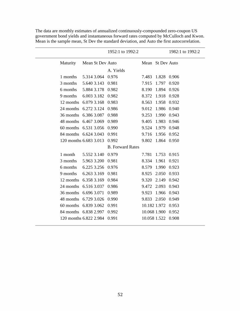
52

The data are monthly estimates of annualized continuously-compounded zero-coupon US

government bond yields and instantaneous forward rates computed by McCulloch and Kwon.

Mean is the sample mean, St Dev the standard deviation, and Auto the first autocorrelation.

1952:1 to 1992:2 1982:1 to 1992:2

Maturity Mean St Dev Auto

Mean St Dev Auto

A. Yields

1 months 5.314 3.064 0.976

7.483 1.828 0.906

3 months 5.640 3.143 0.981 7.915 1.797 0.920

6 months 5.884 3.178 0.982 8.190 1.894 0.926

9 months 6.003 3.182 0.982 8.372 1.918 0.928

12 months 6.079 3.168 0.983 8.563 1.958 0.932

24 months 6.272 3.124 0.986 9.012 1.986 0.940

36 months 6.386 3.087 0.988 9.253 1.990 0.943

48 months 6.467 3.069 0.989 9.405 1.983 0.946

60 months 6.531 3.056 0.990 9.524 1.979 0.948

84 months 6.624 3.043 0.991 9.716 1.956 0.952

120 months 6.683 3.013 0.992 9.802 1.864 0.950

B. Forward Rates

1 month 5.552 3.140 0.979

7.781 1.753 0.915

3 months 5.963 3.200 0.981 8.334 1.961 0.921

6 months 6.225 3.256 0.976 8.579 1.990 0.923

9 months 6.263 3.169 0.981 8.925 2.050 0.933

12 months 6.358 3.169 0.984 9.320 2.149 0.942

24 months 6.516 3.037 0.986 9.472 2.093 0.943

36 months 6.696 3.071 0.989 9.923 1.966 0.943

48 months 6.729 3.026 0.990 9.833 2.050 0.949

60 months 6.839 3.062 0.991 10.182 1.972 0.953

84 months 6.838 2.997 0.992 10.068 1.900 0.952

120 months 6.822 2.984 0.991 10.058 1.522 0.908

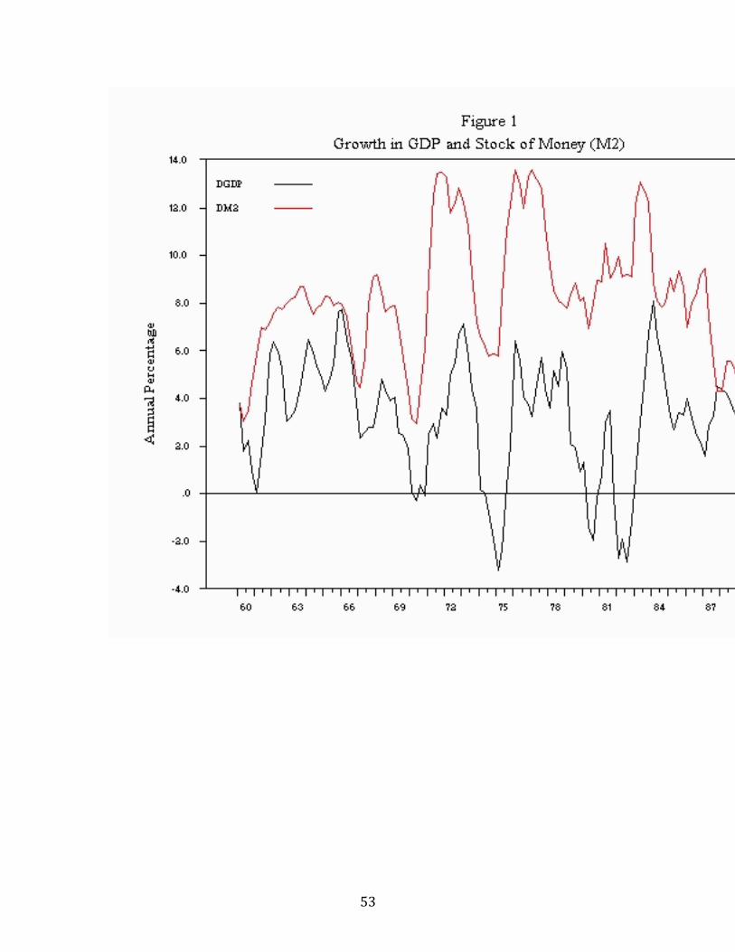
53

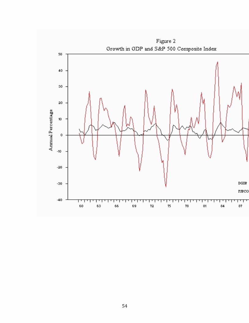
54

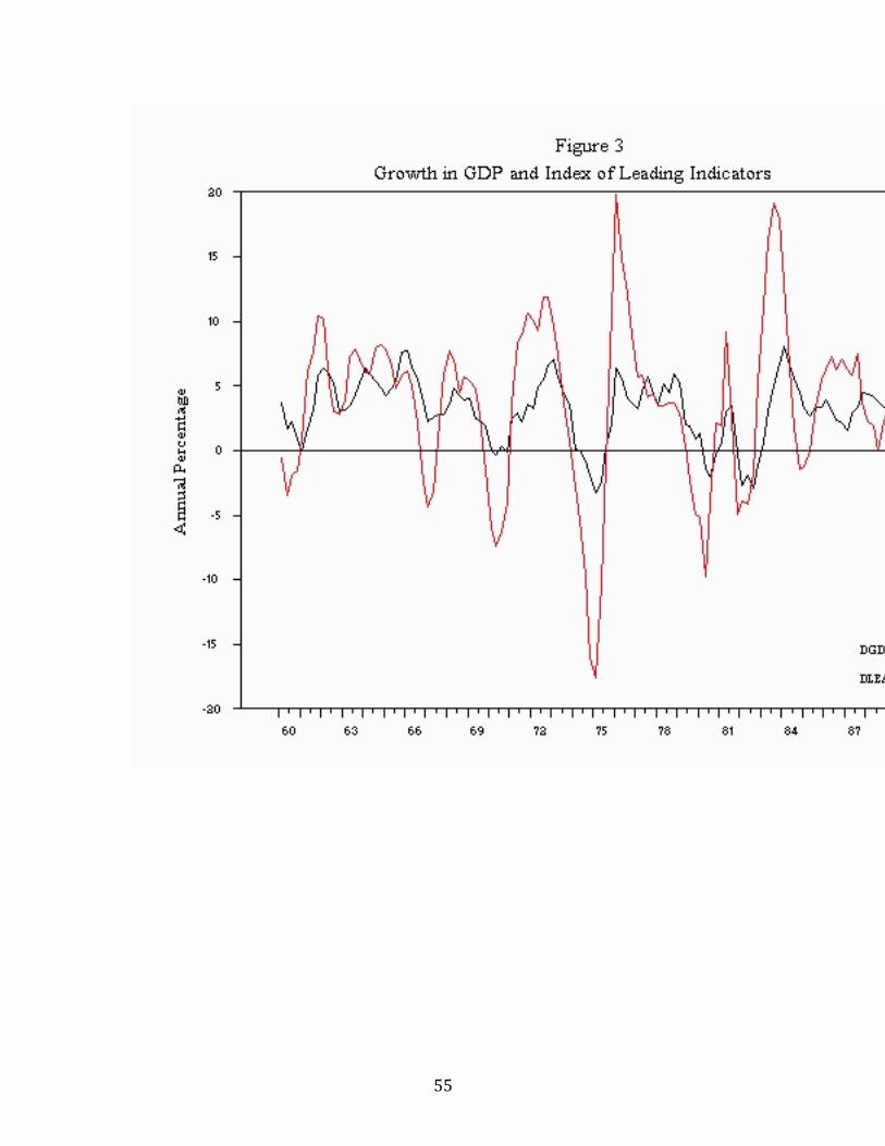
55

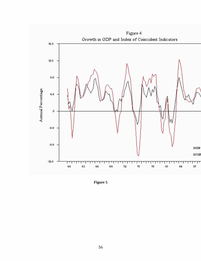
56

Figure 5

57

.

.

.

.

.

.

.

.

Figure 6

58

Copyright: Nouriel Roubini and David Backus, Stern School of Business, New York

University, 1998.

59

Chapter 3. International Indicators

Trade Balance, Current Account and Capital Flows: Balance of Payments Accounts

The Sustainability of Current Account Deficits and Large Foreign Debt: The Role of the

Capital Account

Nominal and Real Exchange Rates and the PPP

Fixed ExchangeRates, Real Exchange Rate Appreciation and Current Account Deficits

Interest Rates and Exchange Rates

Summary

Further Readings

Further Web Links and Readings

We consider in this chapter three international indicators: international trade and payments,

exchange rates, and foreign and domestic interest rates. This will be fleshed out in greater detail later in the course, but I think it's worth taking a look now.

Trade Balance, Current Account and Capital Flows: Balance of Payments Accounts

We start with international trade. We've seen that one measure of an economy's net trade with

the rest of the world is included in the national income and product accounts, net exports. By

this measure, there was a large deficit during the 1980s, and more recently closer to balanced

trade; see Figure 1. There's another popular measure, reported monthly, that indicates that the

US is still running a large deficit: the merchandise trade balance, often called simply the trade

balance. This measure is less comprehensive than net exports, focusing on trade in physical

goods like cars. It ignores trade in services, where the US typically runs a substantial surplus.

These services range from legal and financial products, to custom computer software, to

engineering services provided by Americans to foreign buyers, to foreign "purchases'' of US

education. The merchandise trade deficit, then, is only part of the story. Even worse, the

merchandise trade balance ignores the sophisticated services in which the US has a marked

comparative advantage (and generally a substantial surplus, too).

Another common measure of international payments is the current account, which we denote

CA. This measure is more comprehensive than net exports, and includes net interest

payments on foreign borrowing and lending and miscellaneous "transfers'' between countries.

Our three measures of net US transactions with other countries are pictured in Figure 1 as fractions of GDP. Therefore in summary:

Current Account Transactions:

1. Merchandise Balance = Exports - Imports of Goods

2. Net Exports (Trade Balance, NX) = Merchandise Balance plus Net Exports of Services (or Balance on Goods and Services)

3. Current Account Balance (CA) = Trade Balance + Net Factor Income from Abroad ( = NX + i NFA)

60

[Technical Note: in addition to net exports and the net factor income from abroad, the CA

includes also another item, the net Unilateral Transfers. These are the gifts and grants that the

country received or gave to the rest of the world. So formally, we have: CA = NX + i NFA +

Net Unilateral Transfers].

The current account measures the flow of cash arising from trade and transfers. It also

measures, indirectly, the economy's international financing requirement. If (say) the US has a

100 billion dollar current account deficit, then it must raise 100 billion through some

combination of selling US assets abroad and borrowing from foreign sources. The point (and

this is one of the central messages of the course) is that the cash flows measured by the

current account are mirrored by equal and offsetting financial cash flows, which we refer to

as the capital account. The issue is exactly analogous to the organization of the statement of

cash flows for a firm (as seen in Table 1). A firm with a negative net cash flow from

operations (we see the reverse in the table) must balance this with an equal and opposite

source of cash from financial transactions. The only new feature of the accounts for a country

is the statistical discrepancy, a sign that the numbers collected by the government have some

mistakes in them somewhere.

As shown in Chapter 1, we can use the current account to keep track of changes in the

economy's financial position vis a vis the rest of the world. If NFA is the net stock of foreign

assets held by people in the United States (US ownership of foreign assets, net of foreign

ownership of US assets), then (excepting changes in asset valuation) changes in NFA are equal to the current account:

NFAt+1 = NFAt + CAt .

In fact, the net foreign assets at the beginning of next period (t+1) must be equal to those in

period t plus total national income (GNP) minus the part of national income that is consumed (C and G) or invested (I):

NFAt+1= NFAt + GDPt + it x NFAt - Ct - Gt - It = NFAt + CAt

Note that another way of seeing the relation between the current account and the net foreign

assets of the country is to see the link between the current account of the BP (that records

current transactions, i.e. trade in goods and services and the interest payments on net foreign

assets) and the capital account of the BP (that records capital transactions, i.e. the purchase

and sale of foreign assets). In particular, we will show that the sum of the current account

(CA) and capital account (KA) of the balance of payments is equal to the change in the

official foreign reserves of the country (d(FAX) or:

CA + KA = d(FAX) (1)

Intuitively, the above expression makes sense. Suppose, for a moment, that the change in

official foreign reserves is zero (d(FAX)=0) so that the overall balance of payments (the sum of the current and capital account is zero):

CA+KA=0

61

To see why the above expression must be true, note that if we have a current account deficit,

say CA = -50 < 0), we need a capital inflow (net new borrowing) from the rest of the world to

finance this CA imbalance. Since we are borrowing from the rest of the world, the increase in

our foreign debt is a capital inflow (as foreign residents are buying domestic securities,

bonds, equities, or extend bank credit/loans to domestic agents). Therefore, a current account

deficit (CA= -50 <0) is associated by a matching and equivalent positive capital inflow (KA

= 50 >0) that is represented by a positive item in the Capital Account of the balance of

payments (KA = 50 >0). Since the capital inflow is equal to the negative of the CA deficit

(KA = 50= - CA = -(-50)), we get that CA+KA =0.

Now let us introduce official foreign reserves (of the central bank). Suppose next that the

country is running a $50b current account deficit that needs to be financed with an equivalent

net capital inflow. Suppose, however, that foreign agents are willing to lend only $30b to the

domestic economy, i.e. the positive capital inflow (KA) is only $30b. Then, the only way that

the country can finance its current account deficit (its excess of imports over exports) is to

run down its official foreign assets (i.e. the reserves of the central banks). In other terms, if

foreign agents are not willing to lend funds to domestic agents to finance the excess of

imports over exports, the domestic agents will go to the central bank, purchase foreign

currency from the central banks that they pay for buy paying with domestic currency

(money); then, they will use this foreign currency to pay for the excess of imports over

exports. This set of transactions will lead to a reduction in the stock of official foreign assets

(foreign reserves) of the central bank. The change in the stock of official foreign reserves

(d(FAX)) will therefore be equal to excess of the current account deficit relative to the capital inflow or:

d(FAX) = CA + KA =

-20 = -50 + 30

To derive more formally the above balance of payments identity (1) note that:

NFA = Foreign Assets (FA) - Foreign Liabilities (FL) =

= Domestic Assets Abroad - Foreign Assets in the Domestic Country =

= Foreign Assets held by Domestic Residents - Foreign Debt owed by Domestic Residents

Let us first distinguish between assets and liabilities of the private sector and the government

sector:

FA = FAP + FAX

FL = FLP + FLG

where FAP are the foreign assets of the private sector and FAX are the foreign assets of the

government sector (the official foreign reserves of the country that are usually held by the

central bank, a government agency). Similarly, the total foreign debt of the country FL is the

62

sum of the foreign debt of the private sector (FLP) and the foreign debt of the government

(FLG).

Let us now define private capital outflows and capital inflows as:

Change in Private Sector Foreign Assets = Private Capital Outflows = FAPt+1 - FAPt =

Change in assets the private sector buys/holds abroad (including the change in loans we

make to foreigners)

Change in Private Sector Foreign Liabilities = Private Capital Inflows = FLPt+1 - FLPt =

Change in liabilities (foreign debt) that the private sector owes to foreigners

Similarly, define government capital outflows and capital inflows as:

Change in Government Sector Foreign Assets = FAXt+1 - FAXt = Change in the official

foreign reserves of the government sector

Change in Government Sector Foreign Liabilities = Government Capital Inflows = FLPt+1 -

FLPt = Change in liabilities (foreign debt) that the government owes to foreigners

Now, we define the capital account of the balance of payments (KA) as:

Capital Account of BP (KA) = Private Capital Inflows + Government Capital Inflows -

Private Capital Outflows

Then:

CAt = NFAt+1 - NFAt = [(FAt+1 - FLt+1)- (FAt - FLt+1)]

= - [(FLPt+1 - FLPt) + (FLGt+1 - FLGt) - (FAPt+1- FAPt)] + (FAXt+1- FAXt) = - KAt

+ d(FAX)t

This implies that:

CAt + KAt = d(FAX)t

Note also that the overall balance of payments, including the changes in official foreign reserves, is by accounting identity, always equal to zero:

BPt = CAt + KAt - d(FAX)t = 0

In fact, when the current account is in a surplus (CA>0), we are on net accumulating foreign

assets: therefore the capital account is in a deficit (KA < 0) and/or we are increasing our

official foreign reserves (d(FAX)>0). Total capital outflows (including the government

accumulation of foreign assets) are greater than capital inflows. When the current account is

63

in a deficit (CA<0), we are on net decumulating foreign assets (or increasing our net foreign

liabilities): therefore the capital account is in a surplus (KA>0) and/or we are losing official

foreign reserves (d(FAX)<0). The overall balance of payments must, by accounting

definition, be always equal to zero because any current account transaction has and equal and corresponding transaction in the capital account or the official reserves of the country.

To give an example, consider the case of Korea in 1996 (all data in billions of US dollars):

Equivalent line

in IMF

International

Financial

Statistics

Trade Balance on Goods -15.3 78acd

Trade Balance on Services -5.3 78add - 78aed

Overall Balance on Goods and Services -20.6 78afd

Net Foreign Income From Abroad: -2.5 78agd-78ahd

of which:

Income paid -5.3 78ahd

Income received +2.8 78agd

Balance on Goods, Services and Income -23.1 78aid

Net (Unilateral) Current Transfers 0.1 78ajd - 78akd

of which:

Transfers made -4.3 78akd

Transfers received +4.4 78ajd

Current Account (CA): -23.0 78ald = 78afd +(78ajd-

78akd) .

Capital Account (KA): +24.4 = 43.6 - 19.2 (Cap. Inflows - Cap.

Outflows) . .

Capital Inflows: 43.6 of which:

Foreign Portfolio investments in Korea 16.7 78bgd (foreign purchases of Korean stocks and bonds)

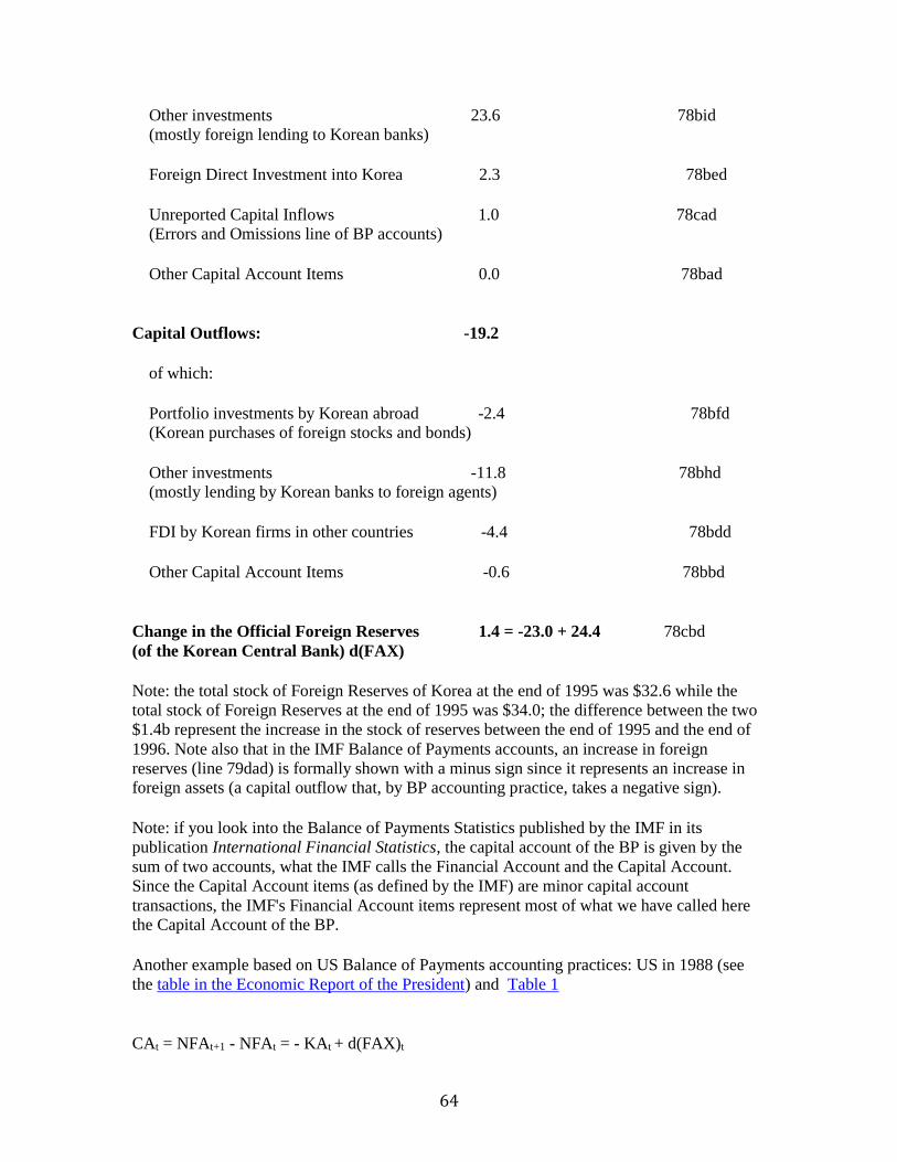
64

Other investments 23.6 78bid

(mostly foreign lending to Korean banks)

Foreign Direct Investment into Korea 2.3 78bed

Unreported Capital Inflows 1.0 78cad (Errors and Omissions line of BP accounts)

Other Capital Account Items 0.0 78bad

Capital Outflows: -19.2

of which:

Portfolio investments by Korean abroad -2.4 78bfd (Korean purchases of foreign stocks and bonds)

Other investments -11.8 78bhd (mostly lending by Korean banks to foreign agents)

FDI by Korean firms in other countries -4.4 78bdd

Other Capital Account Items -0.6 78bbd

Change in the Official Foreign Reserves 1.4 = -23.0 + 24.4 78cbd

(of the Korean Central Bank) d(FAX)

Note: the total stock of Foreign Reserves of Korea at the end of 1995 was $32.6 while the

total stock of Foreign Reserves at the end of 1995 was $34.0; the difference between the two

$1.4b represent the increase in the stock of reserves between the end of 1995 and the end of

1996. Note also that in the IMF Balance of Payments accounts, an increase in foreign

reserves (line 79dad) is formally shown with a minus sign since it represents an increase in foreign assets (a capital outflow that, by BP accounting practice, takes a negative sign).

Note: if you look into the Balance of Payments Statistics published by the IMF in its

publication International Financial Statistics, the capital account of the BP is given by the

sum of two accounts, what the IMF calls the Financial Account and the Capital Account.

Since the Capital Account items (as defined by the IMF) are minor capital account

transactions, the IMF's Financial Account items represent most of what we have called here the Capital Account of the BP.

Another example based on US Balance of Payments accounting practices: US in 1988 (see

the table in the Economic Report of the President) and Table 1

CAt = NFAt+1 - NFAt = - KAt + d(FAX)t

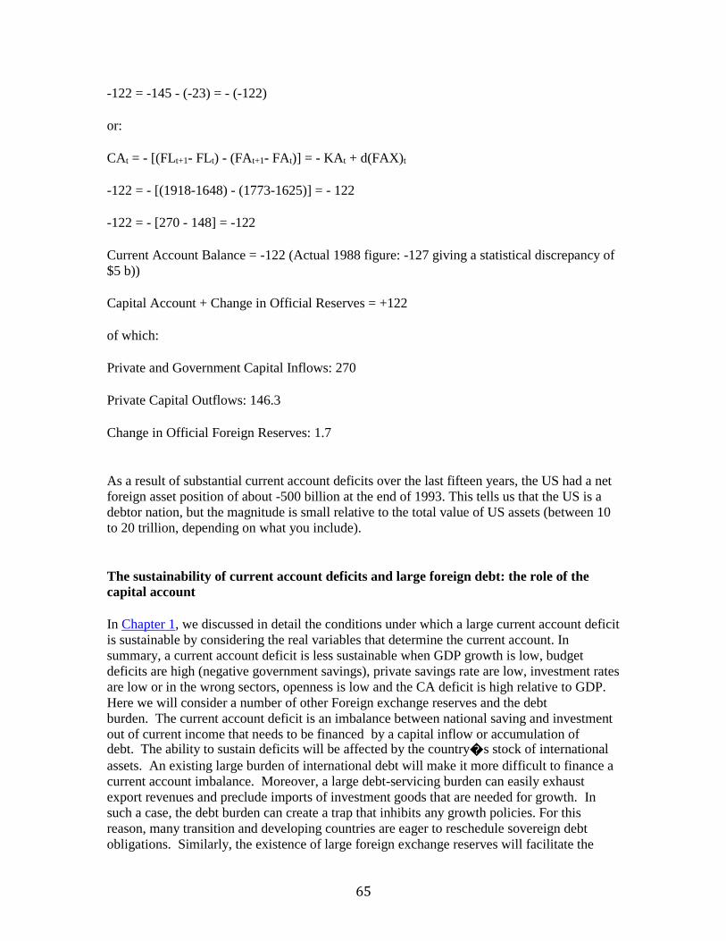
65

-122 = -145 - (-23) = - (-122)

or:

CAt = - [(FLt+1- FLt) - (FAt+1- FAt)] = - KAt + d(FAX)t

-122 = - [(1918-1648) - (1773-1625)] = - 122

-122 = - [270 - 148] = -122

Current Account Balance = -122 (Actual 1988 figure: -127 giving a statistical discrepancy of

$5 b))

Capital Account + Change in Official Reserves = +122

of which:

Private and Government Capital Inflows: 270

Private Capital Outflows: 146.3

Change in Official Foreign Reserves: 1.7

As a result of substantial current account deficits over the last fifteen years, the US had a net

foreign asset position of about -500 billion at the end of 1993. This tells us that the US is a

debtor nation, but the magnitude is small relative to the total value of US assets (between 10

to 20 trillion, depending on what you include).

The sustainability of current account deficits and large foreign debt: the role of the

capital account

In Chapter 1, we discussed in detail the conditions under which a large current account deficit

is sustainable by considering the real variables that determine the current account. In

summary, a current account deficit is less sustainable when GDP growth is low, budget

deficits are high (negative government savings), private savings rate are low, investment rates

are low or in the wrong sectors, openness is low and the CA deficit is high relative to GDP.

Here we will consider a number of other Foreign exchange reserves and the debt

burden. The current account deficit is an imbalance between national saving and investment

out of current income that needs to be financed by a capital inflow or accumulation of debt. The ability to sustain deficits will be affected by the country�s stock of international

assets. An existing large burden of international debt will make it more difficult to finance a

current account imbalance. Moreover, a large debt-servicing burden can easily exhaust

export revenues and preclude imports of investment goods that are needed for growth. In

such a case, the debt burden can create a trap that inhibits any growth policies. For this

reason, many transition and developing countries are eager to reschedule sovereign debt

obligations. Similarly, the existence of large foreign exchange reserves will facilitate the

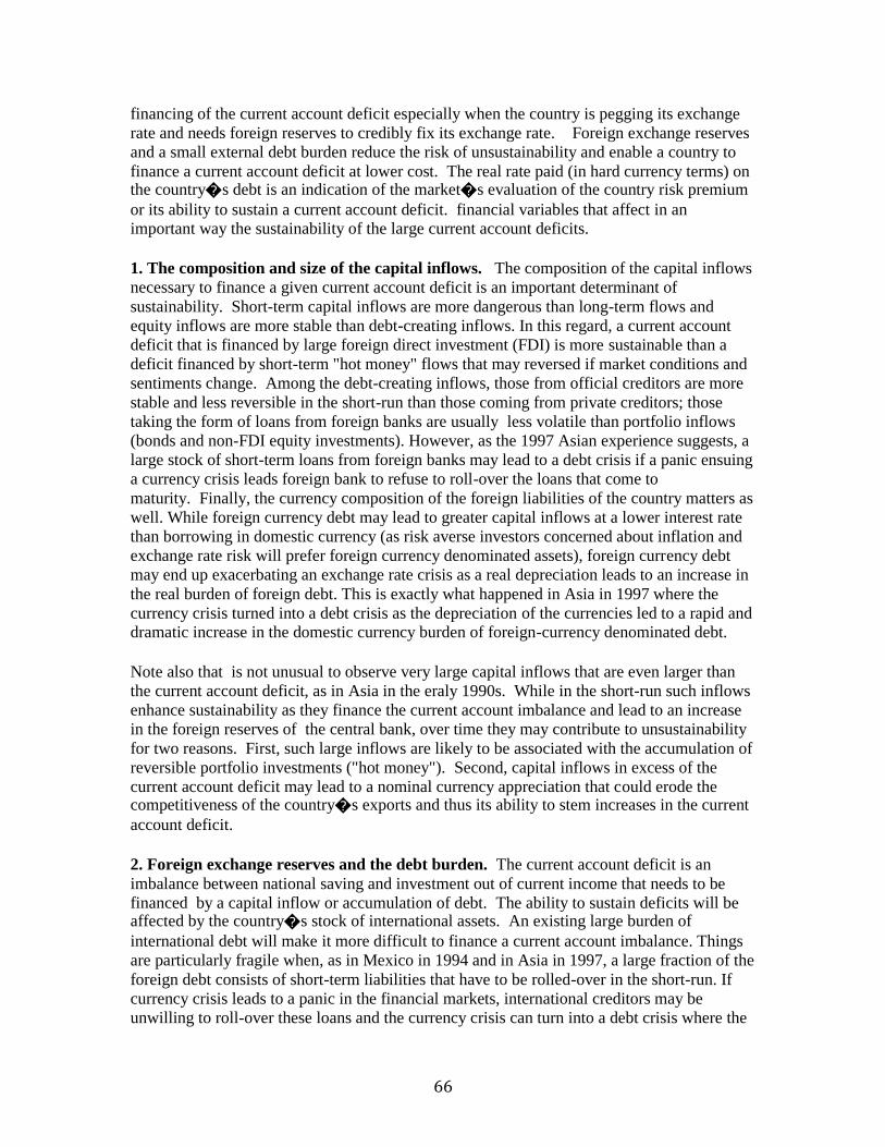
66

financing of the current account deficit especially when the country is pegging its exchange

rate and needs foreign reserves to credibly fix its exchange rate. Foreign exchange reserves

and a small external debt burden reduce the risk of unsustainability and enable a country to

finance a current account deficit at lower cost. The real rate paid (in hard currency terms) on the country�s debt is an indication of the market�s evaluation of the country risk premium

or its ability to sustain a current account deficit. financial variables that affect in an important way the sustainability of the large current account deficits.

1. The composition and size of the capital inflows. The composition of the capital inflows

necessary to finance a given current account deficit is an important determinant of

sustainability. Short-term capital inflows are more dangerous than long-term flows and

equity inflows are more stable than debt-creating inflows. In this regard, a current account

deficit that is financed by large foreign direct investment (FDI) is more sustainable than a

deficit financed by short-term "hot money" flows that may reversed if market conditions and

sentiments change. Among the debt-creating inflows, those from official creditors are more

stable and less reversible in the short-run than those coming from private creditors; those

taking the form of loans from foreign banks are usually less volatile than portfolio inflows

(bonds and non-FDI equity investments). However, as the 1997 Asian experience suggests, a

large stock of short-term loans from foreign banks may lead to a debt crisis if a panic ensuing

a currency crisis leads foreign bank to refuse to roll-over the loans that come to

maturity. Finally, the currency composition of the foreign liabilities of the country matters as

well. While foreign currency debt may lead to greater capital inflows at a lower interest rate

than borrowing in domestic currency (as risk averse investors concerned about inflation and

exchange rate risk will prefer foreign currency denominated assets), foreign currency debt

may end up exacerbating an exchange rate crisis as a real depreciation leads to an increase in

the real burden of foreign debt. This is exactly what happened in Asia in 1997 where the

currency crisis turned into a debt crisis as the depreciation of the currencies led to a rapid and dramatic increase in the domestic currency burden of foreign-currency denominated debt.

Note also that is not unusual to observe very large capital inflows that are even larger than

the current account deficit, as in Asia in the eraly 1990s. While in the short-run such inflows

enhance sustainability as they finance the current account imbalance and lead to an increase

in the foreign reserves of the central bank, over time they may contribute to unsustainability

for two reasons. First, such large inflows are likely to be associated with the accumulation of

reversible portfolio investments ("hot money"). Second, capital inflows in excess of the

current account deficit may lead to a nominal currency appreciation that could erode the competitiveness of the country�s exports and thus its ability to stem increases in the current

account deficit.

2. Foreign exchange reserves and the debt burden. The current account deficit is an

imbalance between national saving and investment out of current income that needs to be

financed by a capital inflow or accumulation of debt. The ability to sustain deficits will be affected by the country�s stock of international assets. An existing large burden of

international debt will make it more difficult to finance a current account imbalance. Things

are particularly fragile when, as in Mexico in 1994 and in Asia in 1997, a large fraction of the

foreign debt consists of short-term liabilities that have to be rolled-over in the short-run. If

currency crisis leads to a panic in the financial markets, international creditors may be

unwilling to roll-over these loans and the currency crisis can turn into a debt crisis where the

67

country risks to default on its foreign debt liabilities. The existence of large foreign exchange

reserves will facilitate the financing of the current account deficit especially when the

country is pegging its exchange rate and needs foreign reserves to credibly fix its exchange

rate. Foreign exchange reserves and a small external debt burden reduce the risk of

unsustainability and enable a country to finance a current account deficit at lower cost. The real rate paid (in hard currency terms) on the country�s debt is an indication of the

market�s evaluation of the country risk premium or its ability to sustain a current account

deficit.

3. Fragility of the financial system. The soundness of the domestic financial system, particularly the banks, has bearing on a country�s ability to sustain a current account

deficit. Capital inflows require a large intermediation role of domestic banks. In fact, as bond

and security markets are not very well developed in many emerging economies (for example

in Asia), a large chunk of the capital inflows financing current account deficits are

intermediated by the domestic banking system. Since firms often cannot borrow directly in

international capital markets, they borrow from domestic banks that in turn borrow from foreign financial intermediaries.

The trouble, however, is that domestic banking crises are common in developing and

emerging economies. More often than not they are the direct result of bad lending practices,

often due to political influences on bank lending or the requirement that banks (which are

often state owned) allocate credit to sustain state owned enterprises. The problem is

exacerbated when the banks source of funds is borrowing from abroad in hard currencies. A

collapse of the banking system has several immediate consequences. Uncertainty and

instability concerning the payments system will quickly stem the inflow of foreign capital

necessary to finance current account deficits. Thus, banking sector fragility can easily be the

proximate cause of an unsustainable current account deficit and a debt crisis, as suggested by

the experiences of Korea, Indonesia and Thailand in 1997-98.

4. Political instability and uncertainty about the economic environment. Political

instability or mere uncertainty about the course of economic policy will have much the same

consequences as banking sector instability. The threat of a change in regime or of a regime

that is not committed to sound macroeconomics policies can reduce the willingness of the

international financial community to provide financing for a current account deficit. Thus, a

deterioration in expectations about the political and financial environment can contribute to a

balance of payments and exchange rate crisis, especially when economic fundamentals are

not very sound. Such shifts in expectations can occur quickly and sometimes without much

warning. Moreover, political instability may lead to larger budget deficits that, in an open

economy, will lead to larger current account deficits

Nominal and Real Exchange Rates and the PPP

Exchange rates. Our second international topic is the exchange rate: the price of foreign

currency. We use the convention that prices of foreign currency, like most prices in this

course, are expressed in dollars. This leads to the confusing result that increases in the

exchange rate are decreases in the value of the dollar, but we'll get used to that soon enough.

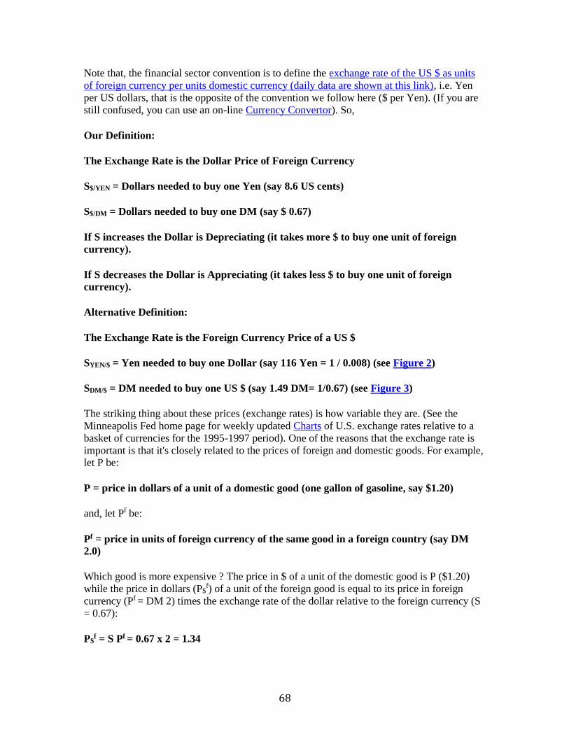
68

Note that, the financial sector convention is to define the exchange rate of the US $ as units

of foreign currency per units domestic currency (daily data are shown at this link), i.e. Yen

per US dollars, that is the opposite of the convention we follow here ($ per Yen). (If you are

still confused, you can use an on-line Currency Convertor). So,

Our Definition:

The Exchange Rate is the Dollar Price of Foreign Currency

S$/YEN = Dollars needed to buy one Yen (say 8.6 US cents)

S$/DM = Dollars needed to buy one DM (say $ 0.67)

If S increases the Dollar is Depreciating (it takes more $ to buy one unit of foreign

currency).

If S decreases the Dollar is Appreciating (it takes less $ to buy one unit of foreign

currency).

Alternative Definition:

The Exchange Rate is the Foreign Currency Price of a US $

SYEN/$ = Yen needed to buy one Dollar (say 116 Yen = 1 / 0.008) (see Figure 2)

SDM/$ = DM needed to buy one US $ (say 1.49 DM= 1/0.67) (see Figure 3)

The striking thing about these prices (exchange rates) is how variable they are. (See the

Minneapolis Fed home page for weekly updated Charts of U.S. exchange rates relative to a

basket of currencies for the 1995-1997 period). One of the reasons that the exchange rate is

important is that it's closely related to the prices of foreign and domestic goods. For example, let P be:

P = price in dollars of a unit of a domestic good (one gallon of gasoline, say $1.20)

and, let Pf be:

Pf = price in units of foreign currency of the same good in a foreign country (say DM

2.0)

Which good is more expensive ? The price in $ of a unit of the domestic good is P ($1.20)

while the price in dollars (P$f) of a unit of the foreign good is equal to its price in foreign

currency (Pf = DM 2) times the exchange rate of the dollar relative to the foreign currency (S

= 0.67):

P$f = S Pf = 0.67 x 2 = 1.34

69

Therefore, the relative price of the foreign good to the domestic good (expressed as RER) is

the ratio,

RER = S Pf / P = 1.34 / 1.20 = 1.166

where S is the (spot) exchange rate. In this example the good in Germany is 16.6% more expensive (when expressed in the same currency) than the same good in the U.S.

Often we would use price indexes, like CPI's or GDP deflators, representing baskets of goods

rather than individual goods. In this case the ratio RER is referred to as the real exchange rate. It indicates how expensive, on average, foreign goods are relative to domestic goods.

If you thought domestic and foreign goods were very similar, and there were few barriers to

trade, then you might expect that when expressed in the same currency their price should be

equal. In this case the real exchange rate would be equal to one and show no variation.

In fact, if the price ratio ever differed from one (as in the example above), then buyers in

Germany would only buy in the cheap country (the US), driving up prices there until foreign

and domestic prices were equal. Thus prices of foreign and domestic goods, expressed in a

common currency, should be about the same, leading the real exchange rate to stay around

one. This theory, applied to the baskets of goods underlying aggregate price indexes, is

referred to as purchasing power parity, (or PPP) since the purchasing power of a dollar is

predicted to be the same in both countries. In other terms, if the goods are identical in both countries and there are no barriers to trade, we would expect that:

P = S Pf

In the example above we had instead:

P =1.20 < S Pf =1.34

So how, can we reach a PPP equilibrium when the relative price differs from unity ? There

are three alternative ways the equilibrium can be restored if we are away from PPP:

1. German prices could fall from DM 2 to DM 1.79 so that

P = 1.20 = S Pf = 0.67 x 1.79

2. US prices may go up from $1.20 to $ 1.34 so that

P = 1.34 = S Pf = 0.67 x 2.00

3. The Dollar/DM exchange rate could appreciate from 0.67 to 0.60 so that

P = 1.20 = S Pf = 0.60 x 2.00

In practice, all of the three effects may be at work in reality. In fact, as initially German

prices are above US ones (when expressed in $), Germans will buy less German goods and

70

demand more of the same good in the US; these two forces will lead to lower prices in

Germany (a lower Pf ) and higher prices in the US (a higher P). Also, as Germans try to buy

more US goods, they have to sell DM in the foreign exchange market in order to buy the

dollars required to pay the US good. This is the mechanism through which the dollar

appreciates and the DM depreciates when we have deviations from the PPP. The simultaneous working of the three effects will eventually lead to the restoration of the PPP.

So what is the evidence on the PPP ? If the PPP holds, the real exchange rate (RER) should be equal to one and constant over time. In fact,

RER = S Pf / P = P / P = 1 (if the PPP holds).

However, we find, when we compute RER using consumer price indexes, that it varies a lot:

prices of (say) Mercedes in particular, and goods in general, are often much different in

Germany and the US, and between any two other countries, as well. At least in the short-

run, the theory of purchasing power parity is a poor approximation. Moreover, most of the

variation is related to movements in the spot rate S. Both of these features are evident in

Figure 4 and Figure 5. In Figure 4 we see that there have been, indeed, large movements in

real exchange rates. In Figure 5 I have divided the real exchange rate into two components.

The ratio P/Pf is the solid line and the spot rate S is the dashed line. If PPP were true, the two

lines would be the same (as PPP implies S = P/Pf). In fact they're much different. What that

means from a business point of view is that fluctuations in currency prices can wreak havoc

on the dollar value of foreign sales, since in general the foreign prices don't change to

compensate. For that reason, an important part of international business is methods of

reducing exposure to currency risk: financial hedging with options and forwards, matching

the currency denomination of revenues and expenses, and so on. There are several courses at

Stern devoted to precisely this issue.

We will discuss in more detail in later chapters the reasons why the PPP does not hold, at

least in the short-run. To anticipate the issues note that, in our example above, we assumed

that the domestic and foreign goods were identical (a gallon of gasoline). However, the RER

represents basket of domestic and foreign goods that can be very different. For example, a

Mercedes car is very different from a GM or Ford car so that we would not expect that prices in the same currency of similar but differentiated products would be equalized.

However, while the PPP may not be holding in the short-run, it should tend to hold in the

long-run: if German prices are systematically higher than U.S. ones, at some point they will

have to fall or US prices will have to go up, or the US $ will have to appreciate (or all of the

above).

To understand the important role of the exchange rate as an adjustment mechanism for relative prices and the trade balance, note the following two points:

1. A depreciation (appreciation) of the domestic exchange rate makes foreign imported

goods more expensive (cheaper) when priced in domestic currency. So a currency

depreciation (appreciation) will lead to a reduction (increase) in the demand for

imported goods as these goods become more expensive (cheaper). This reduction

(increase) in the demand for imports should improve (worsen) the US trade balance.

71

2. A depreciation (appreciation) of the domestic exchange rate makes domestic goods

exported abroad cheaper (more expensive) when priced in a foreign currency. So a

currency depreciation (appreciation) will lead to a increase (decrease) in the foreign

demand for US goods, i.e. an increase (decrease) in US exports as these goods become

cheaper (more expensive) in foreign markets. This increase (decrease) in the US exports

will improve (worsen) the US trade balance.

The above principles work through the effects of changes in the exchange rate on the price in $ of imported goods and the price in foreign currency of US exports.

Specifically:

1. A US Dollar appreciation decreases the price in US $ of imported goods (P$f ) since:

P$f =S Pf . So, a $ appreciation (an decrease in S) will decrease P$

f .

Example:

P$f = S Pf = 0.67 x 2 = 1.34

P$f = S Pf = 0.60 x 2 = 1.20

1. A US Dollar appreciation increases the price in foreign currency (DM) of US goods exported abroad (PDM ) since:

PDM = P / S. So, a $ appreciation (an decrease in S) will increase PDM.

Example:

PDM = P / S = 1.20 / 0.67 = 1.79

PDM = P / S = 1.20 / 0.60 = 2.00

Of course, the converse is true as well: a US $ depreciation makes the price in $ of imported goods more expensive and the price in foreign currency of US exports cheaper.

The above analysis suggests that a depreciation of the nominal exchange rate (S) will lead to

an increase in the relative price of foreign to domestic goods, i.e. it will lead to a depreciation

of the real exchange rate (RER). In fact,

RER = S Pf / P = P$f / P

If we take the price in own currency of domestic and foreign goods (P and Pf ) as given, a nominal depreciation of the exchange rate will also be a real depreciation.

Note that, if the PPP was holding both in the short-run and the long-run, a nominal

depreciation of the domestic currency would not lead to a depreciation of the real exchange

rate. For given foreign prices of foreign goods, a depreciation of the nominal exchange rate

72

would increase proportionally by the same amount the price of imported goods and the price

of domestic goods leaving the real exchange rate unaffected. In this regard, the PPP can be

interpreted both as a theory of the determinant of the exchange rate and as a theory of the

determinant of the domestic price level (or inflation rate). As a theory of the exchange rate, the PPP can be written as:

S = P / Pf

or, we write the expression above in percentage rates of change:

dS/S = dP/P - dPf/Pf

where dx/x is the percentage rate of change of variable x. In the level form, the expression

above says that the exchange rate will be more depreciated if the domestic price level is

higher than the foreign one. In the rate of change form (relative PPP), the expression says that

the exchange rate will depreciate at a % rate equal to the difference between domestic and

foreign inflation. For example, if domestic inflation is 10% while foreign inflation is 4%, the domestic currency should depreciate on average by 6%.

The PPP, as a theory of the determinants of the exchange rate, considers the causality

between P and S as going from domestic inflation to exchange rate depreciation: high

inflation causes high depreciation rates. As a theory of the determinants of the domestic

inflation, instead, the PPP considers the causality as going from the exchange rate to domestic inflation:

dP/P = dS/S + dPf/Pf

The expression above implies that, for given foreign inflation, the domestic inflation rate will

be equal to the foreign inflation rate plus the 'exogenous' rate of depreciation of the domestic

currency. For example, if foreign inflation is 4% and the domestic currency is depreciated by 20%, domestic inflation will be equal to 24%.

Of course, if the PPP does not strictly holds (at least in the short-run), the RER will not be

always equal to one and constant and a depreciation of the nominal exchange rate will also

depreciate the real exchange rate. By how much will the real exchange rate depreciate if the

nominal exchange rate depreciates by x% ? If the domestic price level was completely

independent of the nominal exchange rate, the domestic inflation rate would be totally

unaffected by a nominal depreciation. In this case, the real exchange rate would depreciate by

x% as well. Of course, this is an extreme case where the increase in the price of imported

goods caused by the nominal depreciation does not affect at all the price of domestic goods.

If an x% nominal depreciation leads to an increase in domestic inflation (but by less than the

x% implied by the PPP), the real exchange rate will depreciate but, by less than x%. In fact, by definition:

dRER/RER = dS/S + dPf/Pf - dP/P

73

For example, take Mexico in 1995. Foreign (US inflation) was 3% while the Mexican Peso

depreciated during the year by about 107%. If the Mexican inflation in 1995 has remained at

the 1994 level (about 8%), the 107% nominal depreciation would have corresponded to a real

depreciation of 102% (107 + 3 - 8). However, the large devaluation of 1995 led to an increase

in the inflation rate (as the increase in the price of imported goods led to a surge of domestic

price and wage inflation). As the inflation rate surged to 48% in 1995, the nominal

depreciation of the Peso of 107% corresponded to a smaller real depreciation of 52% (107 +

3 - 48). So the nominal devaluation was effective in changing the relative price of imported

to domestic goods (the RER) in Mexico and led to an improvement in the external balance of

the country: the Mexican trade balance had been in a deficit of 20b US $ in 1994 while it showed a surplus of 3b US $ in 1995.

The above analysis suggest that a currency devaluation is a double sided sword:

1. On one side, it leads to a real depreciation that makes imported goods more expensive,

domestic exports cheaper abroad and leads to an improvement of the trade balance via a fall in imports and an increase in exports.

2. On the other side, a nominal depreciation leads to an increase in domestic inflation that

dampens the effect of the nominal devaluation on the real exchange rate. The faster domestic

inflation adjusts to the change in the exchange rate (i.e. the closer we are to the PPP in the

short-run), the smaller will be the real depreciation following a nominal depreciation, the

smaller will be the improvement in the trade balance and the bigger the increase in domestic

inflation.

Fixed Exchange Rates, Real Exchange Rate Appreciation and Current Account Deficits.

We have discussed above and in Chapter 1 the conditions under which a current account

deficit may or may not be sustainable. We have now to consider the role of exchange rates

and real exchange rate appreciation. A real exchange rate appreciation (from large capital

inflows or any other reason) may cause a loss of competitiveness (as imports become cheaper

and exports more expensive) and a structural worsening of the trade balance which makes the

current account deficit less sustainable. Although the investment-saving imbalance, rather

than a real appreciation, is the proximate source of a current account deficit, the current

account deficit may be less sustainable when accompanied by a real exchange rate

appreciation that leads to a misaligned currency value. Specifically, a real appreciation may

lead to an increase in consumption (of imported goods) and increased imports of capital

goods for investment that result in a worsening of the current account.

Specifically, the large and growing current account imbalances in Asia in the 1990s leads to

the question of whether such imbalances were partly due to a loss of competitiveness

associated with a real appreciation of the exchange rate. In fact, various measures suggest

that many of the countries in Asia whose currencies collapsed in 1997 had experienced

significant appreciation of their real exchange rates in the 1990-96 period.

According to one view (the misalignment hypothesis), the real appreciation observed in Asia

in the 1990s was in part the consequence of the choice of the exchange rate regime (fixed

74

exchange rates) and the ensuing capital inflows; therefore, it represented a loss of real

competitiveness. If this view is correct, the large and growing current account imbalances

were be caused in part by the real appreciation of the currency. This would also imply that

the growing current account imbalances were not sustainable and had to be reversed only

through a process of nominal and real deprecation of the currency, as the one that occurred in 1997.

The above discussion suggests two questions:

1. Were the growing current account imbalances observed in Asia partly casued by movements of the real exchange rate of these countries?

2. Was the real appreciation caused by the choice of the exchange rate regime?

1. Regarding the first question, the data for Asia suggest that the degree of overvaluation of

the real exchange rate was correlated with worsening of the current account: countries with

more overvalued currencies (such as Thailand and Malysia) generally experienced a larger

worsening of the current account; while countries such as China and Taiwan that had

experienced a real depreciation had current account surpluses. An exception was Korea that

had large and increasing current account deficits while its currency had depreciated in real terms in the 1990s.

2. Regarding the second question, in the case of Asia the real appreciation was clearly partly

the consequence of the choice of the exchange rate regime, essentially a fixed peg to the U.S.

dollar. Such a peg led to large capital inflows attracted by favorable interest rate differentials

and the expectation of low exchange rate risk given the policy of stable currency value. Such

inflows prevented currency depreciations even if domestic inflation was higher than world

inflation and at times led to nominal currency appreciation; this, in turn led to a real appreciation that was partly the cause of the large and growing current account imbalances.

While such policy of pegging the exchange rate ensured in many Asian countries ensured the

stability of the nominal exchange rate relative to the US currency, it also had the consequence

that change in the nominal and real value of the dollar relative to the Japanese Yen and the

European currencies had the consequence of affecting the real exchange rate of the Asian

currencies pegged to the US dollar. Specifically, the dollar was on a downward nominal trend

relative to the yen and mark betweeen 1991 and 1995 reaching a low of 80 yen per dollar in

the spring of 1995. During that period, the Asian currencies pegged to the U.S. experienced a

real depreciation of their currencies, as they were depreciating relative to the Japanese and

European currencies. However, after the spring of 1995, the dollar started to rapidly

appreciated relative to most world currencies (the yen/dollar rate went from 80 in the spring

to 1995 to over 125 in the summer of 1997, a 56% appreciation). As a consequence, the

Asian currencies that were tied in nominal terms to the dollar also experienced a very rapid real appreciation.

Note also that a real appreciation of the currency will occur when the exchange rate is pegged

and used as a nominal anchor for monetary policy (as it has been in most Asian countries) if

the initial domestic inflation rate is above the world one and it does not converge rapidly to

the world infaltion rate. In fact, while fixing the exchange rate is a fast way to disinflate an

75

economy starting with a higher inflation rate, pegging the exchange rate will not reduce the

inflation rate instantaneously to the world level. The reasons why inflation will not fall right

away to the world level are several; 1) PPP does not hold exactly in the short tun since

domestic and foreign goods are not perfectly substitutable. So domestic firms will reduce the

inflation rate when the exchange rate is pegged but may not push it immediately down to the

world level. 2) Non-tradable goods prices do not feel the same competitive pressures as

tradable goods prices, thus inflation in the non-traded sector will fall only slowly. 3) Since

there is significant inertia in nominal wage growth, wage inflation might not fall right away

to the world level. Many wage contracts are backward looking and the adjustment of wages

will occur slowly. Also, in countries where there is formal indexation of nominal wages,

wage inflation is based on past (higher) inflation rather than current (lower) inflation; so this

inertia in the wage setting in the economy means that wage inflation will remain above the world rate.

If domestic inflation does not converge immediately to the world level when the exchange

rate parity is fixed, a real appreciation will occur over time. This appreciation of the real

exchange rate implies a loss of competitiveness of the domestic economy: exports become

more expensive relative to imported goods; this worsens the trade balance and the current

account over time. Even small differentials between domestic and foreign inflation rates can

compound rapidly into a substantial real appreciation. Therefore, the problem of anti-

inflation stabilization policies that use the fixed exchange rate as the policy tool to fight

inflation is that fixed rates lead to a real exchange rate appreciation and to a significant

worsening of the current account. While the Asian countries had not experienced the large

inflation rates of some Latin countries, their inflation rates were usually above those of the

OECD group; therefore a policy of pegged parities might have contributed to the real appreciation observed in the 1990s.

Note that, while a real appreciation is more likely to occur (and persist) when the currency is

pegged to a fixed exchange rate, misalignments of the real exchange rate may also occur

under a regime of managed floating exchange rates unless the central bank follows a crawling

peg policy of targeting the real exchange rate. Nominal and/or real appreciation under a

managed float may occur as a result of large capital inflows. Such inflows may have diverse causes:

1. Optimism about an economy that has successfully started to stabilize and structurally reform its economy.

2. Short-term speculative capital flowing to countries with interest rates higher than world

rates and fixed exchange rates.

In both instances, speculative capital inflows may prevent the nominal depreciation of the

currency necessary to maintain a stable real exchange rate in the presence of persistent

differentials between domestic and foreign inflation.

Technical Caveat: Attempts to prevent a nominal appreciation through foreign exchange

intervention (in the absence of capital controls) may not be able to prevent the real

appreciation. If the interventions are not sterilized, monetary growth will increase and lead to

higher domestic inflation that in turn causes a real appreciation; if they are sterilized,

76

domestic interest rates remain high, capital inflows continue and the pressure towards a

nominal appreciation persist. This is why controls on capital inflows have been suggested as a way to stem inward inflows causing the real appreciation of the domestic currency.

For more on the causes and effects of real appreciations, read Chapter 8 of the lecture notes.

Interest Rates and Exchange Rates

We also see substantial differences in interest rates across countries. In late January of 1992,

for example, the rate on three-month eurodollars at Bankers Trust was 4.19% (annual rate).

[This differs a little from the 3-month treasury bill rate of 3.83 on the same date because T-

bills are exempt from state and local taxes, banks are riskier than the federal government, and

the rates are computed somewhat differently.] The analogous rate on Deutschemark-

denominated deposits at the same bank was 9.52%, a large premium. You might guess that

this reflects the market's expectation that the DM would fall in value relative to the dollar,

and eat up the interest difference in currency losses. That would be a good guess, but you'd

be wrong. As we'll see shortly, you are generally better off (for major currencies) investing in the higher interest rate security, even though the interest is paid in a different currency.

The Covered Interest Parity Condition (CIPC) We'll start with a relation called covered interest parity condition, which says that interest

rates denominated in different currencies are the same once you "cover'' yourself against

possible currency changes. The argument follows the standard logic of arbitrage used

endlessly in finance. Let's compare two equivalent strategies for investing one US dollar. The

first strategy is to invest one dollar in a 3-month eurodollar deposit. After three months that

leaves me with (1+i) dollars, where i is the dollar rate of interest expressed as a quarterly rate (the annualized rate of 4.19% divided by 4).

The second investment strategy has a number of steps. The first is to convert the dollar to

DMs, leaving us with 1/S DMs if S is the spot exchange rate in $/DM. The second step is to

invest this money in a 3-month DM deposit, earning the quarterly rate of return if (f for

foreign again). Here if is the annualized rate of return 9.52% divided by 4. That leaves us

with (1+if)/S DMs after three months. We could convert at the spot rate prevailing three

months from now, but that exposes us to the risk that the DM will fall. An alternative is to

sell DMs forward. In January 1992 we know we will have (1+if)/S DMs that we want to

convert back to dollars. With a three-month forward contract, we arrange now to convert

them at the forward rate F expressed, like S, as $/DM. This strategy leaves us with (1+if)F/S

dollars after three months.

Thus we have two relatively riskless (to the extent that Bankers Trust, the source of these

numbers, pays off on its deposits) strategies, one yielding (1+i), the other yielding (1+if)F/S.

Which is better? Well, if either strategy had a higher payoff, you could short one and go long

the other, earning extra interest with no risk. Of course, Bankers Trust isn't in the business of

letting you take their money this way, so they make sure that these prices are set so that the returns are equal:

(1 + i) = ( 1 + if) F/S

77

It's not hard for them to do, since all of these markets are pretty much run by banks, who are

not in the business of giving money away. We call this equation (and those like it for other maturities) the covered interest parity condition (CIPC).

Example. Here's what the numbers looked like in January 1992. As we said, i= (4.19 %

divided by 4), if = (9.52% divided by 4), S=0.6225 (62 cents per DM), F=0.6114 (so it's

cheaper to buy DMs forward than spot). You can verify that covered interest parity works up

to the accuracy of our numbers. That's generally the case: unless you're a big player and can

manage the bid/ask spread to your advantage, you can view this relation as the truth. It's not

often that economics works this well, so remember this. The covered interest parity can be also written in a simpler form. In fact:

(1 + i) = ( 1 + if) F/S = ( 1 + if) [ 1 + (F-S)/S] = ( 1 + if) [ 1 + fp] = (1 + if+ fp + if fp)

where fp (the forward premium) is the percentage difference of the forward rate from the spot rate. Since the term (if fp) is close to zero, this parity condition becomes approximately:

i = if + fp

i.e. the domestic interest rate is equal to to the foreign rate plus the forward premium. This

gives you a simple rule: if the domestic interest rate is above the foreign rate by x%, the

forward exchange rate (for the maturity equivalent ot the interest rate) will be above (i.e. depreciated relative to) the spot rate by x%.

Note that, as long as there are no restrictions on international capital flows and as long as the

domestic and foreign asset have the same risk characteristics, the covered interest parity

condition must always hold purely as a no-arbitrage condition. In fact, if the CIPC was

not holding it would be possible for agents to make a potentially infinite amount of pure

arbitrage (i.e. riskless profits). To see that, consider the following example based on actual

data from February 13, 1997. That day we had:

iu = 5.5% on a 3-month Eurodollar deposit (annualized rate)

ij = 0.5% on a 3-month Euroyen deposit (annualized rate)

SYEN/$ = 124.4 (Spot Yen per dollar exchange rate)

FYEN/$ = 122.85 (3-month forward exchange rate)

Therefore on that day the CIPC was holding as:

(1+ 0.005/4) = (1+ 0.055/4) 122.85/124.4

Suppose now that, for some reason, that day we had FYEN/$ = 124.4 rather than the actual 122.85 rate. In this case the CIPC would have not held that day since:

(1 + ij ) > ( 1 + iu) FYEN/$ / SYEN/$.

78

We will show that in that case a forward arbitrage strategy would have led to unlimited

riskless profits. Such strategy is as follows:

1. Borrow in Japan an amount of Yen equal to 124.4 billion at a 0.5% (annualized) interest rate for 3 months (quarterly rate of 0.125% = 0.5%/4)

2. Buy US$ spot with your 124.4b Yen to get $ 1b.

3. Invest the $ 1b in a 5.%% US T-bill for three months (3-month return is 1.38% = 5.5% /4).

4. Sell $ 1.00125 b [= $1b (1+ 0.00125)] forward to buy forward Yen in an amount equal to

Yen 124.55b (=124.4 (1+0.00125)). You need these Yen in 3-months to pay back your Yen borrowings with interest.

Then, in 3 months:

The return on the US investment is $ 1.0138b (= $1b (1 + 0.0138))

Use $ 1.00125 b to pay for your forward Yen contract and pay pack your Yen borrowing

Net Arbitrage Profits from the entire operation: $ 1.0138b - $ 1.00125 b = $ 12.55 million

Now if you borrow then times more your arbitrage profits would be $125.5m rather than 12.55m; and so on.

This cannot be an equilibrium as every investor will have an incentive to follow the forward arbitrage strategy described above. As every investor will do the same:

Sell $ forward Buy Yen Forward

We would get an appreciation of the Forward Yen/$ rate down from 124.4 to 122.85, the equilibrium rate that restores the CIPC. In fact, when:

FYEN/$ = 122.85, Arbitrage Profits are Zero as:

ij - iu = = (FYEN/$ - SYEN/$)/SYEN/$ .

0.125% -1.38% = -1.25% = (122.85 - 124.4)124.4 = -1.25%

Therefore, the instantaneous behavior of all agents in the foreign exchange rate market

guarantees that the CIPC hold moment by moment; otherwise, free riskless arbitrage

opportunities would be available.

The Uncovered Interest Parity Condition (UIPC) If you cover your foreign positions with a forward contract, that sense there's no point

worrying about whether to invest in dollars or DMs. But what if, in strategy two, you

79

converted at the spot rate in a quarter (three months form now) and took your chances on the

exchange rate? Your return would then be

(1+itf) St+1 / St ,

where by St+1 is the spot rate a quarter (3 months) from now.

Suppose now that agents are risk-neutral, i.e they care only about expected returns. Then,

expected return on investing in a domestic asset for a period (a quarter) is (1 + i) while the expected return (as of today time t) of investing in a foreign asset is:

(1+itf) E(St+1)/St

where is the expectation I have today (time t) of what the spot exchange rate will be a quarter

(3 months) from now. Now, if agents are risk-neutral and care only about expected returns,

the expected return to investing in a domestic asset must be equal to the (uncertain as of

today) expected return on investing in the foreign asset. This is what is called the uncovered

interest parity condition (UIPC):

(1+it ) = (1+itf) E(St+1) / St ,

where E(xt+1) again means the expectation today (t) of the value at time t+1 of the variable x.

Note that this is not a riskless arbitrage opportunity as the ex-post future spot rate may be

different from what we expected it to be. Rearranging the expression above, we can rewrite the uncovered interest parity condition as:

i = if + dSe/S = if + (E(St+1) - St)/St.

where dSe/S is the expected percentage depreciation of the domestic currency. Again, this

gives us a simple rule: if the UIPC holds, a x% difference between the interest rate at home

and abroad must imply that investors expect that the domestic currency will depreciate by x%.

Given that covered interest parity works, uncovered interest parity amounts to saying that the

forward rate today (delivery of currency at time t+1) is the market's expectation of what the

spot rate will be a period from now:

ft = E(St+1).

More generally, since forward contracts can be signed for any maturity:

Ftt+k = E(Ft+k)

where Ftt+k is the forward rate today for delivery of currency at time t+k and E(St+k)is today's

market's expectation of what the spot rate will be t+k periods from now. [For some forecasts

(expectations) of future exchange rates you can check out the home page of Olsen &

Associates ].

80

To see why the UIPC should hold when agents are risk-neutral consider the following

example based on the previous example. Suppose that:

iu = 5.5% on a 3-month Eurodollar deposit (annualized rate)

ij = 0.5% on a 3-month Euroyen deposit (annualized rate)

SYEN/$ = 124.4 (spot Yen per dollar rate)

FYEN/$ = 122.85 (3-month forward exchange rate)

In this case, the CIPC holds and if the expected future exchange rate E(St+1) happens to be

equal to the current forward rate of 122.85, the UIPC holds as well. However, suppose now

that investors expect the future spot rate at time t+1 to be higher than the current forward rate, i.e.:

Et YEN/$(St+1) = 127 > FYEN/$t = 122.85

Then, consider the following Forward Speculation strategy:

Buy $1b forward at the rate 122.85 Yen/$ that is equivalent to:

Sell Yen 122.85b forward at the rate 122.85 Yen/$.

Then, in 3 months, if the actual St+1 turns out to be 127 Yen/$:

1. Buy Yen 122.85b with $ 0.967b (at a spot rate of 127)

2. Receive $ 1b from your forward contract

3. Make a profit of $ 37 million (= 1000m - 967m)

So if the expected future exchange rate is above the current forward rate, all risk-neutral

investors have an incentive today (time t) to buy $ forward and sell Yen forward (as in the

forward speculation strategy described above). This, however, will lead right away to a

depreciation of the time t forward exchange rate Yen per Dollar (FYEN/$) from its initial value of 122.85. This depreciation of the forward rate will continue until:

FYEN/$ = Et YEN/$(St+1) = 127

Once the forward rate has depreciated to 127, the UIPC is restored again. This example

shows that, if agents are risk-neutral, forward speculation always guarantees that the UIPC should hold in equilibrium.

Note however that, unlike forward hedging that relies on the CIPC to cover you from the risk

of unexpected changes in the future exchange rate, forward speculation is risky. In fact,

suppose that the actual future spot rate turns out to be different from the one you expected; in

particular, suppose that the actual St+1 turns out to be 120 Yen/$ rather than the expected 127.

81

Then, you will lose money from your forward speculation strategy since you will need $

1.023b to buy the Yen 122.85b you owe (given your forward contract) and you will receive

back only $1b from the forward contract. Therefore you will suffer a loss equal to 23m

($1,000m - $1,023m). Therefore, whether you make a profit or lose money from forward

speculation depend on the actual realization of the future exchange rate (relative to the current forward rate):

If FYEN/$ < SYen/$,t+1 you profit if you bought $ forward

If FYEN/$ > SYen/$,t+1 you lose if you bought $ forward

Evidence on the UIPC The expectations hypothesis (UIPC together with the CIPC) implies that, if the forward rate

is less than the current spot rate (Ft < St) so that domestic interest rate are lower than foreign

interest rate, we should expect the spot rate to appreciate: E(St+1) < St. What is the evidence

on the uncovered interest parity condition. Is is true that when domestic interest rates are above (below) foreign ones, the exchange rate will depreciate (appreciate) ?

Consider again the UIPC; it implies that the expected depreciation of a currency is equal to the differential between domestic and foreign interest rates:

dSe/S = i - if

Now, we know from the Fisher Condition (see Chapter 2) that high interest rates can be due

to two factors: high real rates or high expected inflation. So, substituting the Fisher Condition

we get:

dSe/S = (r - rf) + (p - pf)

Consider now two cases:

1. Domestic real interest rate are equal to foreign interest rates. In this case, the domestic

nominal interest rate can be above the foreign rate only if the domestic country is expected to

have a higher inflation rate than the foreign country. In this case, it makes sense to believe

that higher interest rate at home will lead to a currency depreciation. In fact, by the PPP,

higher inflation is associated (sooner or later) with a currency depreciation and the higher

interest rate at home reflects only the higher expected inflation of the home country. This

implication seems to be confirmed by the data: countries with high inflation have, on

average, higher nominal interest rates than countries with lower inflation and, on average, the

currencies of such high inflation countries tend to depreciate at a rate close to the interest rate (or inflation) differential relative to low inflation countries.

2. Domestic inflation is equal (or close to) the foreign inflation rate. In this case higher

interest rates at home do not reflect higher domestic inflation but rather higher real interest

rates due for example to a tight monetary policy by the central bank. In this case, we would

expect that high domestic interest rates will be associated with an appreciating currency (as

the high interest rates lead to an inflow of capital to the high yielding country). In fact, the

82

history of the last twenty years (when the major countries switched from the Bretton Woods

system of fixed exchange rates to the current system of market based rates) suggests that, for

period of time when US inflation is close to the German one, the US appreciates (relative to

the DM) when US interest rates are above the German ones. This is a contradiction of the

UIPC but it reflects the effect of high real interest rates on currency values. See a recent

discussion by the chief currency economist for Morgan Stanley for an argument based on this yield effect.

This brings us back to the question of whether the difference in dollar and DM rates reflects a

prediction that the DM will fall. The expectations hypothesis says yes. But 20 years of

experience with floating exchange rates for major currencies suggests that we should expect,

instead, a rise in the DM. That means that our uncovered investment in DMs not only earns a

higher rate of interest, but we can expect, on average, a bonus as the DM rises in value! In

short, good rules of thumb are (i) high interest rate currencies (of countries with low

inflation) generally increase in value and therefore (ii) expected returns are higher in the high

interest rate currency. Right now you'd probably do better to invest in $ bonds, rather than

DM bonds. Many financial firms have international money market funds that do precisely

that.

Determinants of Exchange Rate The UIPC holds only when agents are risk-neutral and therefore care only about expected

returns rather than the riskiness of the assets. However, if agents are risk-averse, they will

require a higher return (a risk premium in order to hold an assets that is considered to be

more risky than another one. In the presence of the a risk premium the interest parity condition will be modified as follows:

it = itf + (E(St+1) - St)/St + RPt

where now RP represents the risk premium on domestic assets; this risk premium could, for

example, represent the risk of default on domestic assets. If such premium is positive, the

return on the domestic asset should be in equilibrium above the expected return on the

foreign assets because agents consider the domestic assets more risky than the foreign one:

the difference between the return on the domestic assets and the expected return on the

foreign asset is exactly given by the risk premium:

it -[itf + (E(St+1) - St)/St] = RPt

Solving the expression above for the current spot rate, we can rewrite the risk-adjusted

interest parity condition as:

St = [E(St+1)] / [ it - itf + 1 - RPt]

This expression shows us all the factors that determine the current spot exchange rate and that can lead to a change in its value.

First, an increase at time t of the expectation that at time t+1 the currency will be more

depreciated leads to a depreciation of the current (time t) spot exchange rate St. In fact,

83

starting from an initial equilibrium, an increase in E(St+1) leads (for a given initial value of St)

to an increase in the expected return on the foreign asset [itf + (E(St+1) - St)/St]; then, agents

will try to get rid of the domestic asset, sell domestic currency and buy foreign currency in

order to buy the foreign asset. This capital outflows out of the domestic economy will lead to

a depreciation of the current spot exchange rate St; such depreciation will reduce the expected return on the foreign asset and restore the interest parity.

Second, an increase at time t of the the foreign interest rate (itf) leads to a depreciation of the

current (time t) spot exchange rate. In fact, starting from an initial equilibrium, an increase in

(itf) leads (for a given initial value of St) to an increase in the expected return on the foreign

asset [itf + (E(St+1) - St)/St]; then, agents will try to get rid of the domestic asset, sell domestic

currency and buy foreign currency in order to buy the foreign asset. This capital outflows out

of the domestic economy will lead to a depreciation of the current spot exchange rate St; such

depreciation will reduce the expected return on the foreign asset and restore the interest parity.

Third, an increase at time t of the the risk premium on domestic assets (RPt) leads to a

depreciation of the current (time t) spot exchange rate. In fact, starting from an initial

equilibrium, an increase in (RPt) leads (for a given initial value of St and it) to a reduction in

the risk-adjusted return on the domestic assets represented by (it-RPt); then, agents will try

to get rid of the domestic asset, sell domestic currency and buy foreign currency in order to

buy the foreign asset. This capital outflows out of the domestic economy will lead to a

depreciation of the current spot exchange rate St; such depreciation will reduce the expected

return on the foreign asset and restore the parity between the risk-adjusted return on the domestic assets and the expected return on the foreign asset.

Fourth, an increase at time t of the the domestic interest rate (it) leads to an appreciation of

the current (time t) spot exchange rate. In fact, starting from an initial equilibrium, an

increase in (it) leads (for a given initial value of St) to an increase in the return on the

domestic asset; then, agents will try to get rid of the foreign asset, sell foreign currency and

buy domestic currency in order to buy the domestic asset. This capital inflow into the

domestic economy will lead to an appreciation of the current spot exchange rate St; such

appreciation will increase the expected return on the foreign asset [itf + (E(St+1) - St)/St] and

restore the interest parity.

The above example show that various factors (an increase in the future expected exchange

rate, an increase in the foreign interest rate and an increase in the risk premium on the

domestic assets) will all lead to a depreciation of of the domestic currency because they lead

to an increase in the expected return on foreign assets or to a fall in the risk-adjusted return

on domestic assets. All these factors, especially the expectation of future depreciation and the

increase in the risk premium on domestic assets, seem to have played an important role in the

rapid depreciation of the Asian currencies in 1997. How could the Asian governments have

prevented these sharp depreciations of their currencies and maintained their exchange rate

pegged to the US dollar? The answer is simple: if exogenous shocks such an increase in the

future expected exchange rate, an increase in the foreign interest rate and an increase in the

risk premium on the domestic assets lead to capital outflows and a pressure on the domestic

currency to devalue, the equation above suggest that the only way to prevent such

84

devaluation is to sharply increase the domestic interest rate to a level that restores the risk-

adjusted interest parity condition.

However, such a policy of high interest rates is problematic since it might prevent a

devaluation but it is also certain to lead to a domestic recession if the domestic interest rate

remains high for long enough. In fact, the monetary tightening and credit squeeze that

follows a sharp increase in domestic interest rates usually lead to a fall in domestic demand

for investment and consumption purposes. This fall in aggregate demand is then followed by

a fall in production and a recession. Therefore, defending a fixed exchange rate parity when

the market is pushing for a currency depreciation may turn out to be very costly in output

terms. This is exactly what happened to Argentina in 1995 where, following the devaluation

of the Mexican Peso in December 1994, speculative capital outflows forced the government

to increase dramatically short-term interest rates to defend its currency board (a rigid fixed

exchange rate system with a 1 to 1 parity of the Argentinean Peso with the US Dollar).

Argentina was then able to avoid a devaluation of its currency but paid a big price with a

severe recession in 1995. A similar situation in currently occurring in Hong Kong where a

sharp increase in domestic interest rates has so far (January 1998) prevented a depreciation of

the Hong Kong Dollar while most of the other regional currencies have been forced to

devalue their currencies. Such high interest rates are, however, leading to a serious slowdown

in the level of economic activity in Hong Kong and might well lead to a recession in 1998.

We will discuss in more detail the causes of currency crises in Chapter 8 of the Lecture

Notes. Read that chapter now if you want an early introduction to currency crises.

Summary

1. Trade Balance, Current Account and Capital Flows.

2. Nominal Exchange Rates, Real Exchange Rates, Absolute and Relative PPP

3. Spot exchange rates and forward exchange rates.

4. Covered interest parity condition, uncovered interest rate parity condition

5. The global business environment is reflected in trade in goods and assets, in prices of these goods, and in interest rates.

Further Readings

The discussion of currency prices and interest parity conditions can be found in

textbooks on investments and international economics such as Krugman and Obstfeld,

International Economics, Chapters 13 and 14.

Further Web Links and Readings You can find more Web readings on the topics covered in this chapter in the course home

page on Macro Analysis and the page on Macro Data sources.

Table 1

A. Statement of Cash Flows. Mack Truck, 1989.

Sources (+) Minuses (-) Uses of Cash (Thousands)

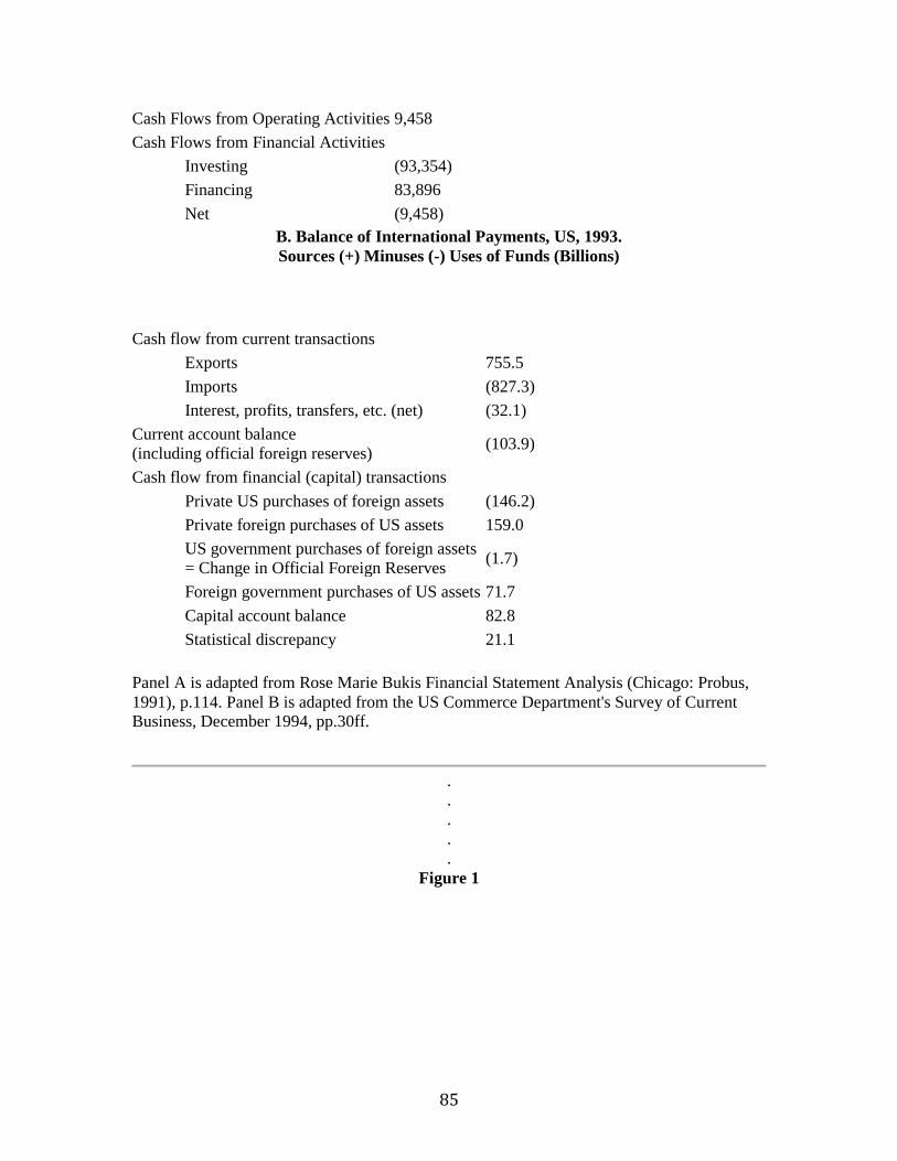
85

Cash Flows from Operating Activities 9,458

Cash Flows from Financial Activities

Investing (93,354)

Financing 83,896

Net (9,458)

B. Balance of International Payments, US, 1993.

Sources (+) Minuses (-) Uses of Funds (Billions)

Cash flow from current transactions

Exports 755.5

Imports (827.3)

Interest, profits, transfers, etc. (net) (32.1)

Current account balance

(including official foreign reserves) (103.9)

Cash flow from financial (capital) transactions

Private US purchases of foreign assets (146.2)

Private foreign purchases of US assets 159.0

US government purchases of foreign assets

= Change in Official Foreign Reserves (1.7)

Foreign government purchases of US assets 71.7

Capital account balance 82.8

Statistical discrepancy 21.1

Panel A is adapted from Rose Marie Bukis Financial Statement Analysis (Chicago: Probus,

1991), p.114. Panel B is adapted from the US Commerce Department's Survey of Current Business, December 1994, pp.30ff.

.

.

.

.

.

Figure 1

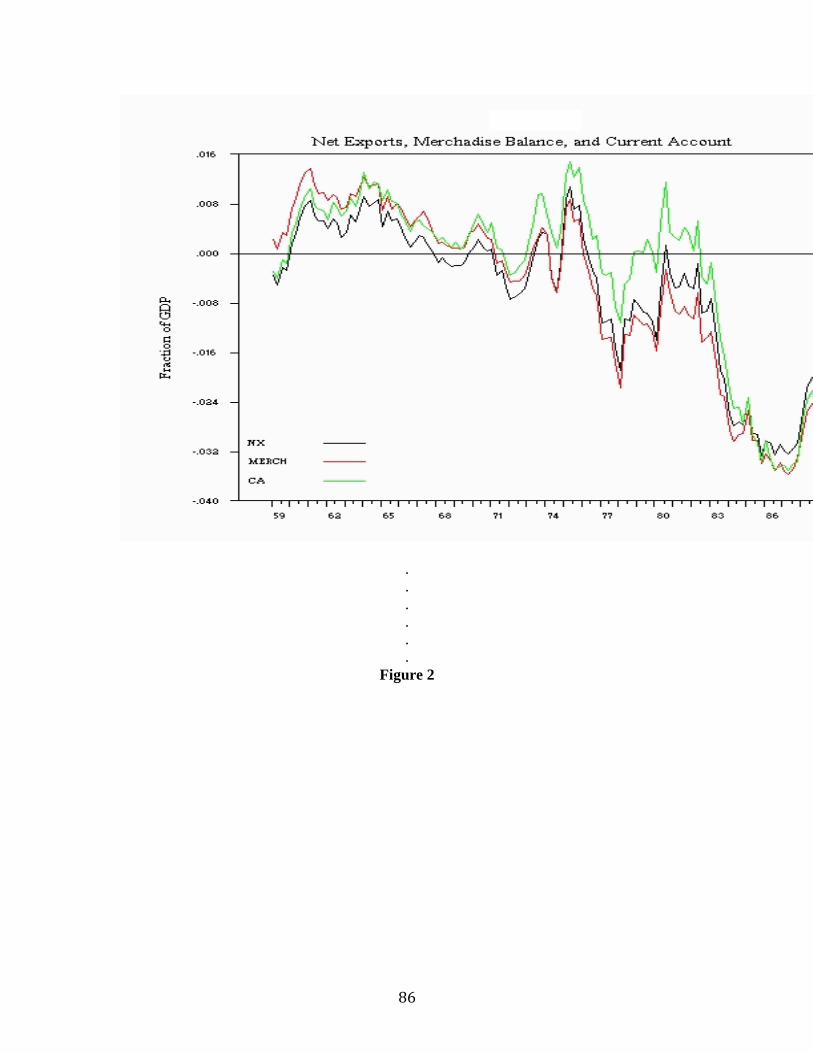
86

.

.

.

.

.

.

Figure 2

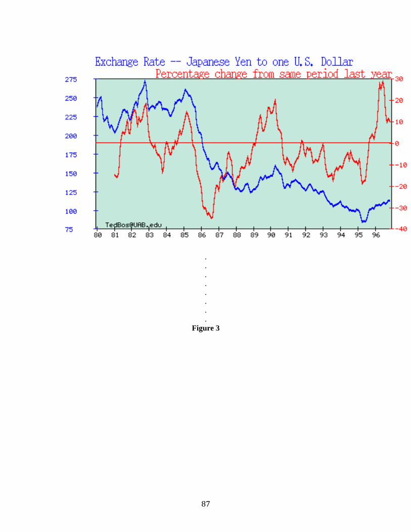
87

.

.

.

.

.

.

.

.

Figure 3

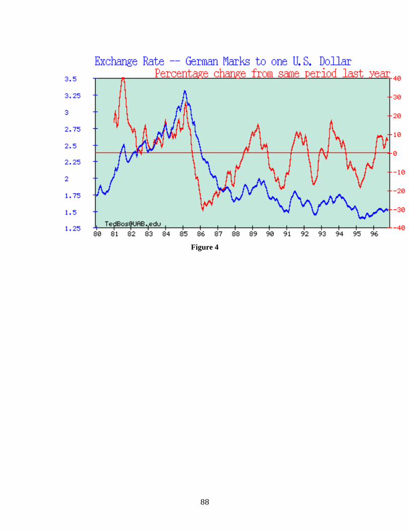
88

Figure 4

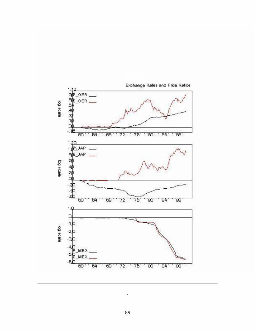
89

.

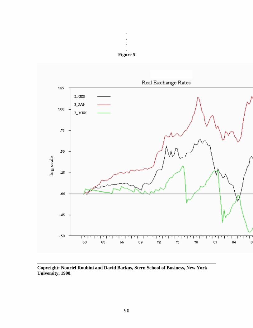
90

.

.

.

.

Figure 5

Copyright: Nouriel Roubini and David Backus, Stern School of Business, New York

University, 1998.

91

Chapter 4. Productivity and Growth

Introduction

Inputs and Outputs: The Production Function

Sources of Growth

The Productivity Slowdown Puzzle

The Mystery of the Vanishing Productivity Growth in the 1990s and Its Post-1995

Resurgence

Returns to Education

Technology

Some Puzzling Examples

Management Strategies: Cooperation and Competition

Policy Options

Summary

Further Reading

Further Web Links and Readings

Productivity and Growth

Perhaps the most striking facts in economics concern the large cross-country differences in

output and income per person. People in the US are, on average, 3 times richer than those in

Mexico, fifteen times richer than people in India, and (when I last looked) about fifteen

percent richer than the Japanese. These differences in levels are matched by large differences

in growth rates. As a start, consider the following data:

Per Capita GDP Average Growth Rate

Country 1960 1985

Argentina 3091 3486 0.5

China 716 2444 4.9

Germany 5217 10708 2.9

Japan 2239 9447 5.8

India 533 750 1.4

Korea 690 3056 6.0

Mexico 2157 3985 2.5

United States 7380 12532 2.1

USSR (RIP) 2951 6266 3.0

[The growth rates are for per capita GDP, expressed as an annual percentage. Data are from

Summers and Heston's Penn World Tables, which is as close as we can get to data that are

comparable across countries---you can imagine, for example, the difficulty of using "market

prices" to value output in China and the USSR. This data applies the same "world" prices to

output quantities in all countries.]

The differences in per capita GDP across countries are enormous, and the differences in

growth rates suggest that rankings of levels can change dramatically. Note, for example, that

Korea and India had comparable levels of income in 1960, while in 1985 Korea's per capita

GDP exceeded India's by a factor of 4. At this rate of growth, per capita GDP doubles every

92

12 years. Clearly there is something going on in Korea that India hasn't figured out yet. Or

consider Italy: In 1870 per capita income was 60 percent less in Italy than in Great Britain,

but after more than a century of growth one-half of one percent larger, Italy has now caught

up. This is the hoary old "power of compound interest" cliché, which shows that even clichés can contain basic truths.

Our objective today is to try to put this into some perspective (which is asking a lot for one

lecture). There are no simple answers, but for a subject this important I think it's useful just to

throw out some ideas. One of the things I find interesting about this subject is that many of the issues that arise when you think about countries also pertain to the performance of firms.

Inputs and Outputs: The Production Function

The central feature of any economy is that economic agents take factor inputs---labor, capital,

and raw materials---and convert them into useful products. Not quite alchemy, but useful

nonetheless. We call this relation between factor inputs and output a production function.

Thus we might write

Y = A F(K,N),

where Y is output (real GNP), K is the stock of physical capital (plant and equipment), and N

is labor (the number and hours of people working). The letter A measures what we will call

productivity. A higher value of A means that the same inputs lead to more output, as clear a

definition of productivity as I can think of. [Despite this, the word productivity is used in

many different ways. When you run across it in other contexts, your first order of business is

to find out exactly what it means.] For future reference, we'll refer to A sometimes as total

factor productivity, to distinguish it from, say, average labor productivity, Y/N.

As we'll see shortly, we owe a lot of the growth in the US economy (and other economies,

too) to increases in A. For now, let's think of things that might affect A. (i) Technological

progress can be thought of as increases in A: invention of the diesel engine, the transistor, the

microchip, penicillin, and so on. (ii) The skill level of the labor force is another thing that

might be incorporated in A. One of the big differences between rich and poor countries is that

the former have better educated and more highly skill workers. For this reason, we would not

expect NAFTA (the North American Free Trade Agreement with Mexico and Canada) to

result in American wages falling to the level of Mexican wages. (I'm afraid Ross Perot was

out to lunch on this one.) (iii) Oil prices. We've seen that an increase in the price of imported

oil may leave us with lower GNP, other things equal, since a greater fraction of gross output

goes to oil, less to capital and labor (hence less value-added). We can think of this as a

downward movement in A (and, in fact, that's what we see in the data). (iv) Weather. A

drought or extreme cold snap might lead to lower output for given inputs. Droughts aren't a

big deal in the US economy, since agriculture is a small part of the economy, but it gives you

the idea that lots of things might affect A. (v) The economic and legal environment might

also play a role in aggregate productivity. Most economists think that competitive markets

play an important role in allocating resources in an efficient manner, and this kind of thinking

is behind many of the changes in the former Soviet Union and Central Europe. Conversely, corruption and red tape are often given much of the credit for India's lethargic performance.

93

Sources of Growth

Productivity is the cornerstone of economic growth. We are richer than our grandparents and

than the average person in the third world primarily because we are more productive.

Productivity also affects our competitive position: the more productive we are the better we

are able to compete on world markets. In short, productivity is the source of the high standard

of living enjoyed by the developed economies relative to the third world or to the same

economies fifty or one hundred years ago.

This section is dedicated to defining and measuring productivity, and using a theoretical

framework to determine the sources of economic growth. The fundamental relation in productivity measurement is, again, the production function:

Y = A F(K,N).

This function says, as we've seen, that we get higher output for three reasons: because more

people are working (higher N), because they have more equipment to work with (higher K),

or because capital and labor are used more productively (higher A, a catchall category). What

I'd like to do is decompose growth in real output Y into components due to each of these

three elements -- an exercise that has come to be called growth accounting. If the production function has the form

Y = A K1/3N2/3,

this decomposition has a particularly simple expression. [Don't ask! The exponents mean that

one third of output is paid to capital in profits, depreciation, etc., and two-thirds to labor,

which is about what we see in the US and many other countries.] Then growth in aggregate output Y is

dY/Y = dA/A + 0.33 dK/K + 0.67 dN/N, (*)

where dX/X represent the percentage rate of change of variable X over the period considered (for example one year):

dX/X = (Xt - Xt-1)/Xt-1

In practice we know all the terms but A, which we compute as a residual. We generally do not measure A directly, which adds to its enigmatic character.

We can, with little change, use this to account for growth in output per worker, Y/N, which is

more directly tied to living standards than output. Given the structure of the production function, this can be written

Y/N = A (K/N)1/3 ,

and growth decomposes into

d(Y/N)/(Y/N)= dA/A + 0.33 d(K/N)/(K/N).

94

What this says is that output per worker can rise for two reasons: because total factor

productivity A is increasing and because the amount of capital per worker, K/N, is increasing.

We can get some idea of why the US economy grew over the last thirty years by examining

the components of (*). Growth of real output over the 1960 to 1985 period was 3.1 percent

per year. [This is higher than the number above, because we are talking about total output

here, not output per capita. There are also some minor differences in how the numbers were

constructed.] How much of this growth was attributable to increases in inputs? From the data

we find that the growth rates of labor and capital over the same period were 1.9 and 3.2

percent, resp. Applying the coefficients as indicated in (*), we find that this gives us about

1.1 (= 3.2 x .33) percent growth per year due to increases in the stock of capital and 1.3 (=

1.9 x .67) percent due to increases in the number of people working. What's left over, so that

the two sides of (*) balance, is about 0.7 percent growth in productivity A. To be honest, it's

not really this easy to separate the three components: many advances in technology show up

in either capital (new and more productive machines) or labor (better trained workers). But

this gives you some idea of how important productivity is in aggregate growth. Figure 1 and

figure 2 present the same data in a different way, as the annual values of (the logarithm of) A

and its rate of change. Note for future reference the spikes: there are large short-term movements in A associated with business cycles.

This emphasis on productivity is well placed, I think, but there are cases in which other

factors are more important. Following World War II both Germany and Japan suffered

massive losses to their capital stocks (think of Kuwait or Iraq following the Gulf War). In the

process of catching up with the rest of the world, they had very high rates of capital growth

that led to high rates of output growth. In the case of Japan, this process continued into the

1970s. To see this, let's do the numbers. From a different dataset (constructed by the OECD)

we have

U.S.

Japan

1970 1985 Growth 1970 1985 Growth

Real Output (Y) 2083 3103 2.66 620 1253 4.69

Capital (K) 8535 13039 2.83 1287 3967 7.50

Employment (N) 78.6 104.2 1.88 35.4 45.1 1.61

Employment is measured in millions of workers, real output and capital in billions of 1980

US dollars. Growth rates are average annual percentage rates.

Digression on growth rates. I've used two properties of logarithms to get these numbers. The

first is that, for any two numbers x and y

log(xy) = y log(x)

here log stands for the natural logarithm (sometimes denoted ln), which is what we'll always

use in this class (no unnatural logs allowed!). In words, the equation says that logarithms

change powers into multiplication. The second property is that the logarithm of 1+x, where x is small, is approximately x:

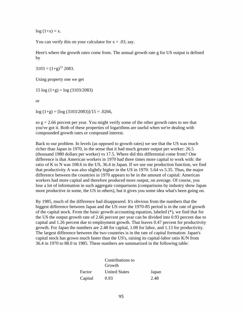
95

log (1+x) = x.

You can verify this on your calculator for x = .03, say.

Here's where the growth rates come from. The annual growth rate g for US output is defined by

3103 = (1+g)15 2083.

Using property one we get

15 log (1+g) = log (3103/2083)

or

log (1+g) = [log (3103/2083)]/15 = .0266,

so g = 2.66 percent per year. You might verify some of the other growth rates to see that

you've got it. Both of these properties of logarithms are useful when we're dealing with

compounded growth rates or compound interest.

Back to our problem. In levels (as opposed to growth rates) we see that the US was much

richer than Japan in 1970, in the sense that it had much greater output per worker: 26.5

(thousand 1980 dollars per worker) vs 17.5. Where did this differential come from? One

difference is that American workers in 1970 had three times more capital to work with: the

ratio of K to N was 108.6 in the US, 36.4 in Japan. If we use our production function, we find

that productivity A was also slightly higher in the US in 1970: 5.64 vs 5.35. Thus, the major

difference between the countries in 1970 appears to be in the amount of capital: American

workers had more capital and therefore produced more output, on average. Of course, you

lose a lot of information in such aggregate comparisons (comparisons by industry show Japan more productive in some, the US in others), but it gives you some idea what's been going on.

By 1985, much of the difference had disappeared. It's obvious from the numbers that the

biggest difference between Japan and the US over the 1970-85 period is in the rate of growth

of the capital stock. From the basic growth accounting equation, labeled (*), we find that for

the US the output growth rate of 2.66 percent per year can be divided into 0.93 percent due to

capital and 1.26 percent due to employment growth. That leaves 0.47 percent for productivity

growth. For Japan the numbers are 2.48 for capital, 1.08 for labor, and 1.13 for productivity.

The largest difference between the two countries is in the rate of capital formation: Japan's

capital stock has grown much faster than the US's, raising its capital-labor ratio K/N from

36.4 in 1970 to 88.0 in 1985. These numbers are summarized in the following table:

Contributions to

Growth

Factor United States Japan

Capital 0.93 2.48

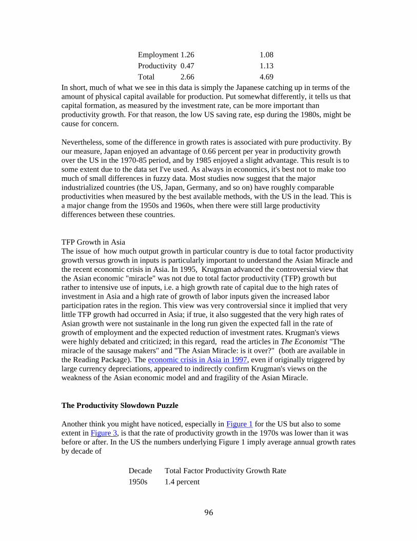
96

Employment 1.26 1.08

Productivity 0.47 1.13

Total 2.66 4.69

In short, much of what we see in this data is simply the Japanese catching up in terms of the

amount of physical capital available for production. Put somewhat differently, it tells us that

capital formation, as measured by the investment rate, can be more important than

productivity growth. For that reason, the low US saving rate, esp during the 1980s, might be

cause for concern.

Nevertheless, some of the difference in growth rates is associated with pure productivity. By

our measure, Japan enjoyed an advantage of 0.66 percent per year in productivity growth

over the US in the 1970-85 period, and by 1985 enjoyed a slight advantage. This result is to

some extent due to the data set I've used. As always in economics, it's best not to make too

much of small differences in fuzzy data. Most studies now suggest that the major

industrialized countries (the US, Japan, Germany, and so on) have roughly comparable

productivities when measured by the best available methods, with the US in the lead. This is

a major change from the 1950s and 1960s, when there were still large productivity

differences between these countries.

TFP Growth in Asia

The issue of how much output growth in particular country is due to total factor productivity

growth versus growth in inputs is particularly important to understand the Asian Miracle and

the recent economic crisis in Asia. In 1995, Krugman advanced the controversial view that

the Asian economic "miracle" was not due to total factor productivity (TFP) growth but

rather to intensive use of inputs, i.e. a high growth rate of capital due to the high rates of

investment in Asia and a high rate of growth of labor inputs given the increased labor

participation rates in the region. This view was very controversial since it implied that very

little TFP growth had occurred in Asia; if true, it also suggested that the very high rates of

Asian growth were not sustainanle in the long run given the expected fall in the rate of

growth of employment and the expected reduction of investment rates. Krugman's views

were highly debated and criticized; in this regard, read the articles in The Economist "The

miracle of the sausage makers" and "The Asian Miracle: is it over?" (both are available in

the Reading Package). The economic crisis in Asia in 1997, even if originally triggered by

large currency depreciations, appeared to indirectly confirm Krugman's views on the

weakness of the Asian economic model and and fragility of the Asian Miracle.

The Productivity Slowdown Puzzle

Another think you might have noticed, especially in Figure 1 for the US but also to some

extent in Figure 3, is that the rate of productivity growth in the 1970s was lower than it was

before or after. In the US the numbers underlying Figure 1 imply average annual growth rates

by decade of

Decade Total Factor Productivity Growth Rate

1950s 1.4 percent

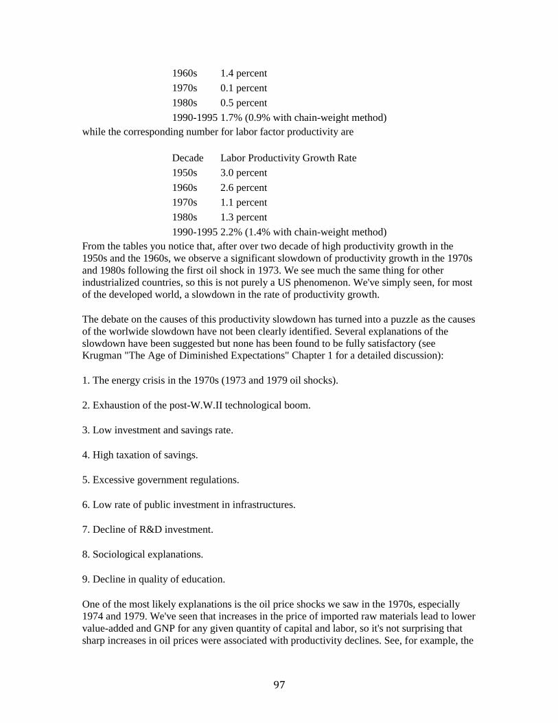
97

1960s 1.4 percent

1970s 0.1 percent

1980s 0.5 percent

1990-1995 1.7% (0.9% with chain-weight method)

while the corresponding number for labor factor productivity are

Decade Labor Productivity Growth Rate

1950s 3.0 percent

1960s 2.6 percent

1970s 1.1 percent

1980s 1.3 percent

1990-1995 2.2% (1.4% with chain-weight method)

From the tables you notice that, after over two decade of high productivity growth in the

1950s and the 1960s, we observe a significant slowdown of productivity growth in the 1970s

and 1980s following the first oil shock in 1973. We see much the same thing for other

industrialized countries, so this is not purely a US phenomenon. We've simply seen, for most

of the developed world, a slowdown in the rate of productivity growth.

The debate on the causes of this productivity slowdown has turned into a puzzle as the causes

of the worlwide slowdown have not been clearly identified. Several explanations of the

slowdown have been suggested but none has been found to be fully satisfactory (see Krugman "The Age of Diminished Expectations" Chapter 1 for a detailed discussion):

1. The energy crisis in the 1970s (1973 and 1979 oil shocks).

2. Exhaustion of the post-W.W.II technological boom.

3. Low investment and savings rate.

4. High taxation of savings.

5. Excessive government regulations.

6. Low rate of public investment in infrastructures.

7. Decline of R&D investment.

8. Sociological explanations.

9. Decline in quality of education.

One of the most likely explanations is the oil price shocks we saw in the 1970s, especially

1974 and 1979. We've seen that increases in the price of imported raw materials lead to lower

value-added and GNP for any given quantity of capital and labor, so it's not surprising that

sharp increases in oil prices were associated with productivity declines. See, for example, the

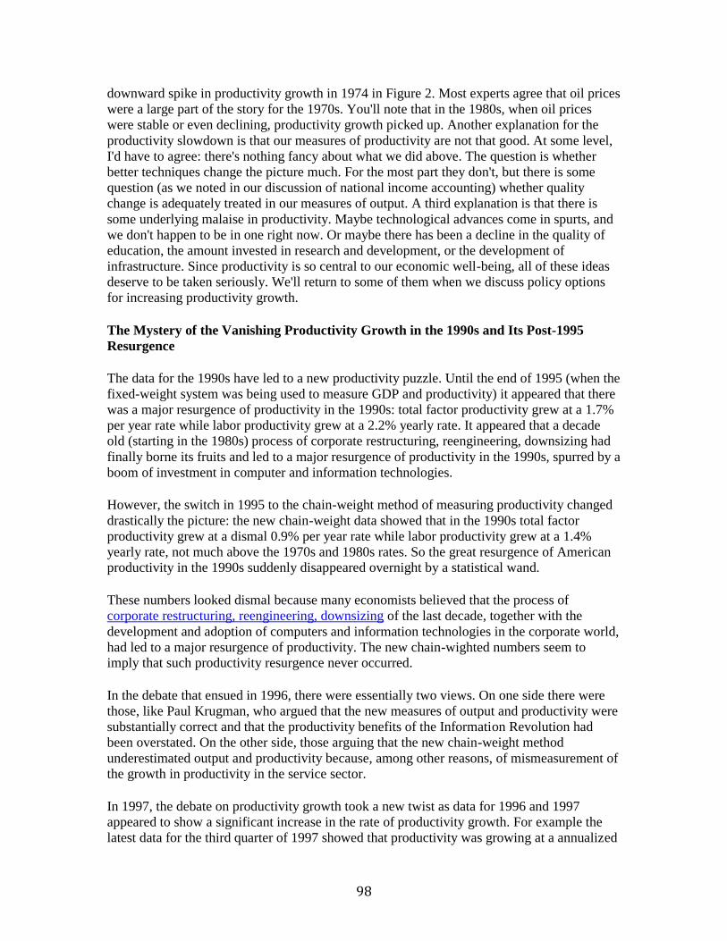
98

downward spike in productivity growth in 1974 in Figure 2. Most experts agree that oil prices

were a large part of the story for the 1970s. You'll note that in the 1980s, when oil prices

were stable or even declining, productivity growth picked up. Another explanation for the

productivity slowdown is that our measures of productivity are not that good. At some level,

I'd have to agree: there's nothing fancy about what we did above. The question is whether

better techniques change the picture much. For the most part they don't, but there is some

question (as we noted in our discussion of national income accounting) whether quality

change is adequately treated in our measures of output. A third explanation is that there is

some underlying malaise in productivity. Maybe technological advances come in spurts, and

we don't happen to be in one right now. Or maybe there has been a decline in the quality of

education, the amount invested in research and development, or the development of

infrastructure. Since productivity is so central to our economic well-being, all of these ideas

deserve to be taken seriously. We'll return to some of them when we discuss policy options

for increasing productivity growth.

The Mystery of the Vanishing Productivity Growth in the 1990s and Its Post-1995

Resurgence

The data for the 1990s have led to a new productivity puzzle. Until the end of 1995 (when the

fixed-weight system was being used to measure GDP and productivity) it appeared that there

was a major resurgence of productivity in the 1990s: total factor productivity grew at a 1.7%

per year rate while labor productivity grew at a 2.2% yearly rate. It appeared that a decade

old (starting in the 1980s) process of corporate restructuring, reengineering, downsizing had

finally borne its fruits and led to a major resurgence of productivity in the 1990s, spurred by a

boom of investment in computer and information technologies.

However, the switch in 1995 to the chain-weight method of measuring productivity changed

drastically the picture: the new chain-weight data showed that in the 1990s total factor

productivity grew at a dismal 0.9% per year rate while labor productivity grew at a 1.4%

yearly rate, not much above the 1970s and 1980s rates. So the great resurgence of American productivity in the 1990s suddenly disappeared overnight by a statistical wand.

These numbers looked dismal because many economists believed that the process of

corporate restructuring, reengineering, downsizing of the last decade, together with the

development and adoption of computers and information technologies in the corporate world,

had led to a major resurgence of productivity. The new chain-wighted numbers seem to imply that such productivity resurgence never occurred.

In the debate that ensued in 1996, there were essentially two views. On one side there were

those, like Paul Krugman, who argued that the new measures of output and productivity were

substantially correct and that the productivity benefits of the Information Revolution had

been overstated. On the other side, those arguing that the new chain-weight method

underestimated output and productivity because, among other reasons, of mismeasurement of the growth in productivity in the service sector.

In 1997, the debate on productivity growth took a new twist as data for 1996 and 1997

appeared to show a significant increase in the rate of productivity growth. For example the

latest data for the third quarter of 1997 showed that productivity was growing at a annualized

99

rate of 4.0% in the business sector and a whopping 9.3% in the manufacturing sector (see the

BLS Web Site for the latest productivity report). While the annualized growth rate data might

be distorted by a particular good quarter, the actual quarter-on-quarter annual rates of growth

showed similar large increases of productivity growth: the actual productivity growth

between the third quarter of 1996 and the third quarter of 1997 was 2.4% for the business

sector and 4.6% for the manufacturing sector, well above the dismal rates of 1.0% observed

in the early 1990s and close to the high rate of the 1960s. These new data led a number of

authors to argue that we had entered in a new era of sustained productivity growth; one heard

a lot of talk about a "New Economy" where a "New Paradigm" of high growth and low

inflation holds. The homepages on the New Economy on Productivity Growth in the 1990s

present an introduction to this recent debate. For a critique of the New Economy hypothesis, see two recent articles by Paul Krugman, one on Slate, and the other on Fortune magazine.

Returns to Education

Everyone has his or her own pet theory about what increases productivity and that's as it

should be. This is not something with one simple answer, it's a complex combination of many

factors. I want to mention a few, though, to give you a concrete idea what might underlie our

catch-all aggregate productivity measure. One factor that we've seen can be important is the

rate of investment: in Japan, for example, a higher rate of investment led to greater growth in

the stock of capital and, using the numbers from the previous section, an advantage relative

to the US of about 1.5 percent per year higher output growth [this is the contribution of K I'm

talking about: 1.5 = 2.48 - 0.93.]

Another factor is education, which you can think of as investment in people, or what

economists call "human capital." There is lots of evidence, at the levels of both countries and

individuals, that education is associated with productivity. As a rule, countries that invest the

100

most in education also tend to be the richest and have the highest rates of growth of per capita

output. Note the growth rate effect: not only are countries with more education richer, they also seem to grow faster.

Education has clear benefits to individuals, too, as your presence at Stern probably indicates.

This includes formal schooling, job training, and work experience. A huge number of studies

has established that each year of school tends to raise one's wage between 5 and 7 percent, on

average. The numbers vary depending on the quality of school, the type of education, and so

on, but there's little doubt that more highly educated workers are better paid and, unless firms are throwing their money away, more productive.

There is a clear connection between education and our catch-all productivity measure. Let us

say, to be specific, that educated workers are essentially like extra quantities of uneducated

workers. For example, suppose a "standard" worker with a high school diploma has a

productivity of one (this is just a benchmark). Then a worker with one year of college is

worth, from the studies cited above, about 1.06 standard workers. An increase in the average

education level of the workforce by one year then leads to an increase in the effective labor force, N, of 6 percent. From our production function,

Y = A K1/3 N2/3 ,

we see that this leads to about a 4 percent increase in output and measured productivity [1.04

= 1.062/3]. In short, education shows up directly in aggregate productivity, and its effects are large.

One current fear in the US is that the quality of education has deteriorated in the last twenty

years. This shows up in lower test scores and in frequent complaints by college teachers that

their students are not as well prepared for college courses as they used to be. This is not just a

problem of social policy. Companies in the US and elsewhere spend an enormous amount of

money on worker training. Viewed another way, the increase in private sector training

suggests that learning is no longer confined to schools or to the young. It's a continuing

process.

Technology

Another factor underlying productivity growth is invention and innovation narrowly defined-

--roughly speaking, the men and women in the white lab coats. One way to raise productivity

is to spend money on research and development, which many firms do in a big way. Bristol-

Myers-Squibb, for example, owes much of its recent success to the development of a new

drug for heart patients, a product of generous expenditures on scientific research. Corning has

grown with new developments of glass technology, like fiber optics. The US, on the whole, is

the world leader in pure science and thus, you would think, the leader in development of new

technologies. The trick here is to take basic scientific advances and convert them into

profitable ventures. By all reports the US is not as good at the second step as it is at the first,

while for the Japanese it's the reverse. This is overly simplistic, of course. The main point is

that it takes more than Einstein to generate aggregate productivity growth.

101

One of the troubling trends in the US in recent years has been a decline among US firms in

R&D expenditures, patent applications, and other technology indicators. If this trend continues, some fear adverse long term effects on US productivity growth.

Some Puzzling Examples

You get the idea, by looking at data and using common sense, that the way to grow faster is

to invest in physical capital, human capital, and "knowledge" or "technology." On the whole,

I'd say that's right as far as it goes. Nevertheless, there are some striking examples of cultures

that were advanced technologically but never translated that advantage into economic gain.

Two examples I want to mention here are the Arab world in the middle ages and China circa

1400. I'm not an expert on either case, but I think here even a little bit of knowledge is useful

(and hopefully not too dangerous). [See Joel Mokyr's The Lever of Riches (Oxford, 1991) if

you're interested in the details, it's a fascinating book.] More relevant, perhaps, is that issues

at the national level are replayed at the firm level.

China. In many aspects of technology China was much more advanced prior to 1400 than

Europe. Mokyr mentions: (i) Agriculture: rice cultivation, the iron plow, and so on made

Chinese agriculture much more productive than Europe's. (ii) Iron: the Chinese had blast

furnaces for casting iron in 200 BC, Europe not until late 1300s. (iii) Ship-building and

navigation: the great voyages of the European explorers were predated by the Chinese who,

inexplicably, prohibited foreign exploration just as the Europeans got moving. There are

many other examples (paper, porcelain, the cross-bow, gunpowder), too. On the whole, they suggest a culture with advanced technology in both pure and applied areas.

In short, China was technologically advanced in 1400, but this didn't lead to an industrial

revolution. It's not clear why, but a leading hypothesis is that the centralized system of

government was prone to malfunction with inadequate leaders. An ambitious leader could

encourage innovation and development, or throttle it completely. Regardless of the

explanation, it's clear that it takes more than technology to produce sustained growth in output and productivity. Science and technology alone won't do it.

The Arab World. Maybe some other time. The general idea is that they had better

understanding of math and some aspects of technology than the Europeans in the middle ages and before, yet didn't develop, as Europe did, into a successful industrial society.

I could name some other examples. Argentina was as rich as almost any country in the world

in 1890, but is far from it now. Japan, on the other hand, has grown dramatically from shortly

after the Meiji restoration (1868) to the present, truly a remarkable and, I think,

unprecedented achievement. In 1868 they were internationally isolated but still a highly

educated society, and thus in a good position to capitalize on Western technology once they

were exposed to it. Britain, on the other hand, developed more quickly than France in the

18th century, despite a substantial disadvantage in pure science. They were experts, however, in practical engineering (eg, the steam engine).

This lesson applies to firms, too: advanced technology often fails, for a variety of reasons, to

translate into business success. A striking case is IBM, who for years had the best pure and

applied research. The corporate culture, however, did not exploit these advantages as well as

102

they might have. One example is RISC based computing, the basis for the exploding work

station market. IBM invented this technology in the mid-1970s, but lagged far behind Sun

and other smaller companies in bringing it to market. Evidently technology alone isn't

enough. Another example is GM. Although technology is arguably more important in

manufacturing than in services (and in modern economies services are increasingly

important), the advances GM has made are the result more of management methods than

technology. GM's experiment in robotics is termed by Maryann Keller (Rude Awakening,

HarperCollins 1989, ch 10) as "an experiment that failed," and most observers agree. A

similar point is made by Womack, Jones, and Roos in The Machine that Changed the World

(HarperCollins, 1991). Their figure 4.11 (p 97) compares Ford's Atlanta assembly plant with

GM's Fairfax plant. They found that the GM plant, despite a higher degree of automation, had

substantially lower productivity than the Ford plant. They attributed the difference to design (the GM car had many more parts) and plant organization.

In short, good economic performance, for both countries and firms, appears to involve

features of the economic and social structure that are difficult to define, let alone measure.

We shouldn't be surprised, then, that strategies for raising productivity and growth cover almost every aspect of economic and corporate organization.

Management Strategies: Cooperation and Competition

One of the things you might guess is that firms must invest in new technologies to stay

competitive, perhaps by supporting large research laboratories. And that's probably right in

some cases. But some of the greatest innovations in management and productivity

enhancement concern, instead, changes in the ways in which people are organized. Consider

your typical acronym with a Q in it: SQC (statistical quality control), TQC (total quality

control), QFD (quality function deployment), etc. The basic ideas here concern not

technology in the narrow sense of scientific breakthroughs, but organizing management and

workers to operate more effectively as a team. These management issues are, in my opinion,

at least as important as the advances in technology narrowly defined.

One of the interesting trends in management philosophy has been toward a greater emphasis

on cooperation. The increased weight placed on group work at Stern is an example you may

have noticed. At some level the benefits of cooperation are obvious: you should have the

quarterback and the wide receiver running the same play. In modern management the

suggestion is that there must be active cooperation among the entire production team, from

assembly line workers on up to the CEO. Most of these methods require active participation

by the people on the line to work, since they are the closest to the process and thus know the

most it (hard as that is for senior management to believe). (The center, for example, might

know more about what the opposing lineman are doing than the quarterback.)

As an economist I find this emphasis on cooperation fascinating, because we tend to focus on

competition---in some ways, the antithesis of cooperation. Deming, for example, argues that

firms should have a small number of suppliers, because only then can they enforce quality

standards. The competitive approach, followed by US automobile companies for years, is to

use many suppliers, so that you can use competition among them to keep the price low. So

who's right? I think most people would agree that competition can be an effective tool. The

former Soviet Union, for example, would probably have been more productive if incentives

103

had led to greater competition among individuals and firms to supply goods and services.

And at IBM, competition between divisions, rather than enforced cooperation with the

mainframe division, might have spared them their poor performance in non-mainframe

businesses. But some management studies suggest that competition between workers in

similar jobs can actually lower productivity. Or that competition among students in a course

can reduce the value of their educational experience. The question is where you draw the

line. Should IBM be one firm or many? Should Citibank centralize its loan operations, or

have several competing divisions? Should computer manufacturers join "cooperative"

research programs or go it alone?

The question of where to draw the line between cooperation and competition is not one with

a simple answer, but it's one of the basic issues in business and economic policy. For

management it involves strategic decisions (enter a new business alone or with a joint

venture?), performance appraisal (should individual members of a team be rated and

rewarded differently, which might foster competition but discourage cooperation?), etc. For

policy it involves questions of anti-trust (treatment of joint ventures to allow more

cooperation), tariffs (should we protect ourselves from foreign competition?), and foreign

investment (should we restrict foreign purchases of hi-tech firms, a restraint of international competition?).

Economists, by and large, find that competition among firms has been useful. But maybe

there should be room for cooperation, too. The tension between these two forces is a

continuing theme in management, and I think you'll find that it reappears in your

management courses in other forms.

Policy Options

Growth and productivity are great buzz words in Washington and around the world these

days, partly because they're like motherhood (it's hard to be against them) and partly because

the experience of the 1970s and early 1990s suggests that continued growth isn't automatic.

But what do you do? Depending on your view of cooperation and competition, you might

argue that more or less government involvement is called for. The argument for less

government is that free market forces lead to efficient production and low prices for

consumers. In this sense, excessive government "interference" gets in the way of the

operation of the market system. But the history of successful nations generally includes

examples of active government involvement, esp in infrastructure and education, as well as

examples of relatively free markets. This is yet another example where simple answers don't

do justice to the evidence. You should be thinking, then, for each of these issues whether you

think changes in government policy would lead to better economic performance. I'll focus on

the US, but most of the same issues arise in other countries, too.

Saving and investment. The first item on most lists is that we could do more to encourage

investment, either directly through tax incentives (reduced disencentives?) or indirectly

through incentives to increase saving. Recall that saving and investment are connected

through the identity: S = I + CA. Generally CA is small relative to I and S, as we have seen,

so most investment is financed through domestic saving. We might guess, therefore, that

policies to raise saving will also raise investment. The question is how to do this. The 1989

Economic Report of the President suggested a cut in the capital gains tax, lower corporate tax

104

rates, higher limits on IRA contributions, and (this may be the big one) a smaller federal

government deficit. Missing from their proposal is something many economists think is the

largest distortion in the US tax code: the favorable tax treatment of housing. What seems to

happen in the US is that we invest a disproportionate amount in housing, rather than plant

and equipment. Since it's the latter that makes us more productive, we may have a lower

standard of living (but nice houses!) as a result. It's unlikely that preferential treatment of

housing will disappear in the US, but expanded tax-sheltered saving plans are a possibility. We will discuss more these issues in Chapter 5.

Education. Another method of boosting productivity is to invest in people, which has payoffs

to both the individuals and the economy as a whole. The evidence we've seen suggests that

this can have large returns. The question is how to go about it. I see this as primarily a management issue: how to deliver high quality education on a large scale.

Infrastructure. One of the most important things governments can do, it seems, is make sure

the economy has a good infrastructure, esp transportation and communication. Some of this

is done by the private sector, but in most countries at least part is the responsibility of the

government. Good roads, for example, make it possible for firms to centralize production and

exploit economies of large scale production. Communication equipment is vital in many

fields (think of finance: where would you be without up-to-the minute information).

Historically these have been US strengths, the question is whether we have allowed our

roads/airports to deteriorate in an effort to save money short term, or fallen behind in the

adoption of new communication technology (a fiber optic network). We may find that

investment in these things has large payoffs. The question is which ones.

Scientific research. The US has, over the last fifty years or more, been the world leader in

pure science (often, though, with imported talent). If you look at expenditures on what is

called research and development narrowly defined (the people in the white coats again), the

US spends as much as anyone (measured as a fraction of GDP). But unlike (say) Japan or

Germany, part of this money is spent on military applications, and only has civilian value by

accident. When we subtract the military, we spend somewhat less than these two countries.

We just got done arguing that basic science isn't enough, but that's not to say that it's not

useful. So one of the things we might ask ourselves is whether we should be doing more to encourage research, both publicly and privately funded.

Taxes. One of the things you often hear in the US is that high tax rates discourage good

economic behavior (saving, for example). That may be true, but the US is, on the whole, a

low-tax country. The success of Germany and Japan, where taxes are higher, on average,

suggest that taxes aren't our major problem. In fact, we might be better off with somewhat

higher taxes and better services (choose from the list above). What might be true, though, is

that the structure of the US tax system is inefficient, that we are discouraged from saving and

encouraged to put too much of our wealth in real estate. We might come back to this later in Chapter 5 (but let me warn you now that there is no consensus on this).

That's the A-list. A few other things have gotten attention in the US recently, and maybe

they're important. Health care, for example, has gotten to be such an important factor in

hiring by firms and job decisions by individuals that we have to do something about it (but

what?). It seems to me that almost anything would be an improvement. A second issue is the

105

torts system, which may discourage innovation by saddling firms with large and highly

uncertain liabilities in new product development. The question is how to balance the

incentives for innovation with the incentives to provide safe products. Third, there is some

concern that US anti-trust law, particularly the treble damages aspect, may discourage firms

from adopting joint projects. The evidence here, though, is that large projects are not

generally more effective than small ones, so this may be a red herring (despite the recent

wave of cooperation in computing, like that between Apple and IBM). Moreover, large

Japanese firms, when you look at them closely, show no particular desire to cooperate, so

that's not their secret.

What these policies tell you is that everything is a productivity issue. You don't have to get

them all right, but you must get enough of them right to continue to enjoy growth in

aggregate productivity and wages. Any country that doesn't faces the possibility of becoming

the next Argentina or, as a less extreme example, Great Britain. There are no simple answers, but the stakes are big enough to make the question worth thinking about.

Summary

1. Growth in output comes from increases in factor inputs and growth in productivity

(the letter A in our production function). A major reason why Japan has grown more

rapidly than the US over the last thirty years has been their larger rate of investment

in physical capital (I/Y).

2. Productivity is related to investment in education, research and development,

management techniques, and simple experience...

3. ...but there are a number of examples of societies that were technologically but not

economically advanced. Evidently technology is not enough, you also need a

social/political/cultural/legal environment that fosters its application.

4. Analogously, many productivity increases at the firm level reflect management and

organization of people more than advances in pure science.

5. A variety of national policies are likely to lead to higher productivity: education,

transportation and communication infrastructure, basic and applied research, and

clearly defined property rights.

Further Reading

For data on growth and productivity see the WEB sites listed in the home page on Macro

Data and Information. The most recent version of the Summers-Heston data used at the start

of the chapter is available over the Internet from the NBER's Web site.

There's been a lot of work on productivity at the level of both firms and countries. With

regard to the former, half the books in the business section of most bookstores include the

word quality. Andrea Gabor's The Man Who Discovered Quality is an interesting and highly

readable review of Deming's work. With regard to national productivity, Williamson's article

("Productivity and American leadership," Journal of Economic Literature, March 1991) is a

little difficult, but will give you a good idea of the range of economists' opinions on sources of growth both historically and around the world.

Further WEB Links and Readings

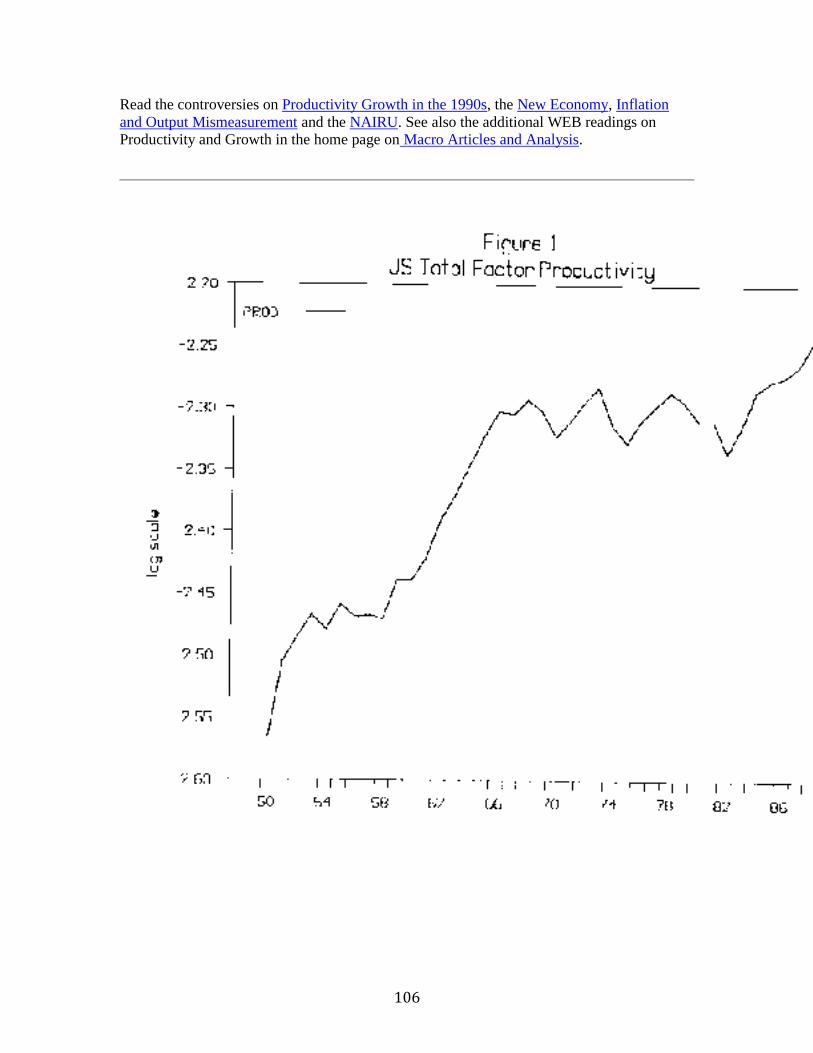
106

Read the controversies on Productivity Growth in the 1990s, the New Economy, Inflation

and Output Mismeasurement and the NAIRU. See also the additional WEB readings on Productivity and Growth in the home page on Macro Articles and Analysis.

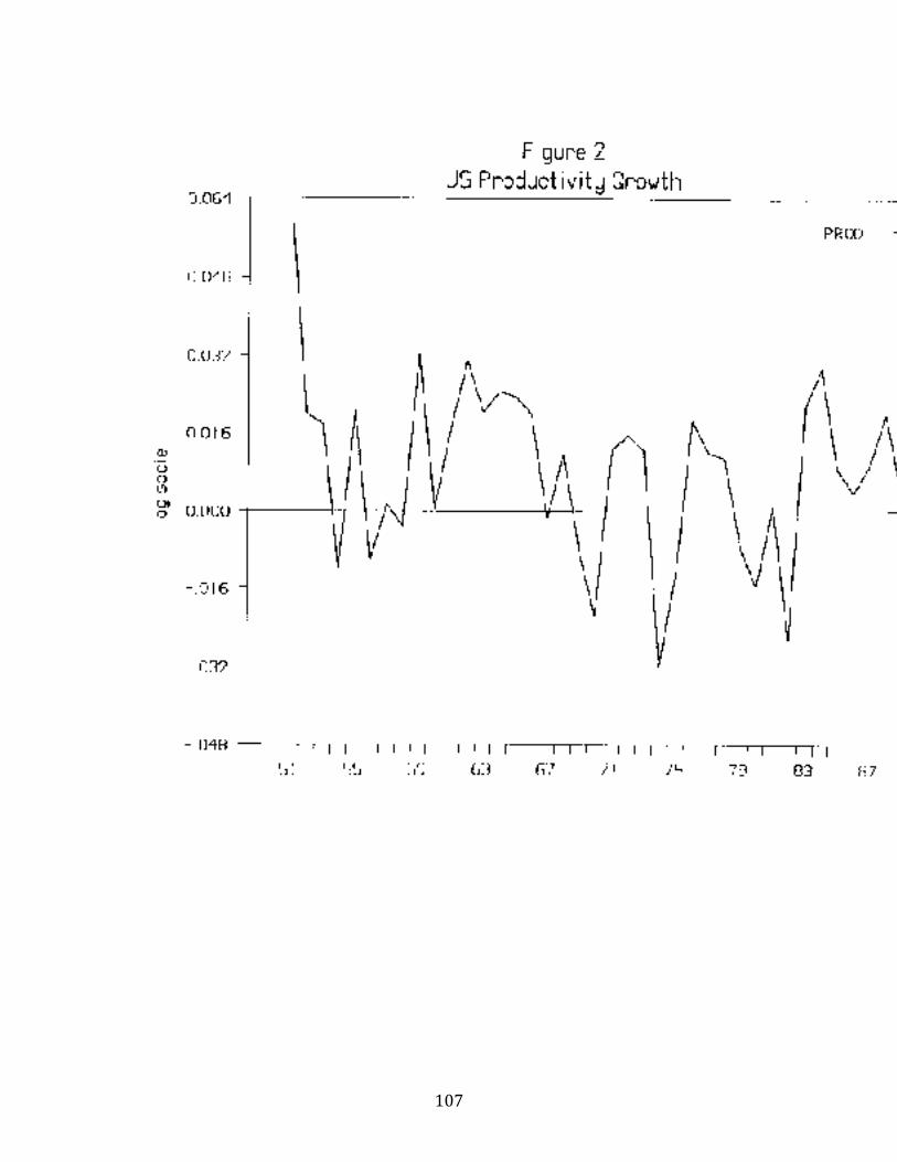
107

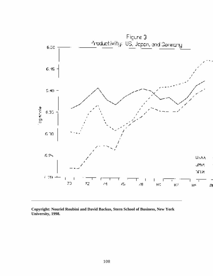
108

Copyright: Nouriel Roubini and David Backus, Stern School of Business, New York

University, 1998.

109

Chapter 5. Output and Real Interest Rates

On Theory in Macroeconomics

The Production Function Again

The Labor Market

The 1974-5 Oil Price Increase

Saving, Investment and the Rate of Interest

Short-Run Equilibrium and Long-Run Dynamics

Application: Are Low Real Interest Rates Good for the Economy?

Application: Voodoo Economics or Supply Side Economics

International Borrowing and Lending and the Current Account

Application: Is a Trade Deficit Bad ?

Application: Roots of the 1980s Trade Deficit

Application: Real Interest Rate in the 1990s

Application: Does Government Spending Raise Output

Summary

Further Web Links and Readings

We've seen, so far, that economies grow at different rates and experience short-term

fluctuations that we've dubbed business cycles. We'd like to go beyond that, though, and say

something about why we observe these things and what we might do to encourage better

macroeconomic performance. What we need is a theoretical framework for thinking about

these issues. Over the next few weeks we're going to examine two versions of a

macroeconomic theory, labeled Classical and Keynesian, that emphasize different aspects of

macroeconomic life. These models are often presented as competitors. I think you'll find

instead that they are complementary, and provide different perspectives on the aggregate

economy. Roughly speaking, the Classical theory is aimed at the long run (say, two years or

longer) and the Keynesian theory at the short run (less than two years), though the distinction

isn't that tight. You'll also find that the two theories share many common elements, so a lot of what we learn with the Classical theory applies to the Keynesian theory as well.

On Theory in Macroeconomics

We're going to dedicate the next few weeks to theory. You may have only a practical interest

in macroeconomics, so let me explain what I mean by theory and why I think you'll find it

useful. We could start by looking up "theory" in the dictionary. I did this and found

(Webster's no 2): "lacking verification or practical application". That's not quite what I have

in mind. I think of theory as a system for organizing and thinking about the world. One

analogy is a filing system for organizing facts and insights. Once you have such a system a

wide range of seemingly unrelated facts start to fall into place. Another analogy for theory is

simplification, like a mental shortcut or a memory device. Both of these aspects of theory are

crucial: organization and simplification. I think you'll find that a lot of different things come

together once you have an organized way of thinking about them. One further advantage of a

sound theoretical framework is that it may be able to deal with situations yet unseen.

By way of motivation, let me report the comment of a member of Stern's Board of Overseers,

the CEO of a large corporation. He said: "Theory is power." What he meant by this, I think,

is that people who understand how things work at a deep level will be able to influence and

110

control those who do not. It's a personal advantage in your business and career. It's certainly

been true of my career: my most marketable skills are my technical skills.

But back to our regularly scheduled programming. In this course I want to give you three

complementary organizing devices: a long run "Classical" theory, a short run "Keynesian"

theory, and an appreciation for accounting relations connecting seemingly different things.

As I said, these are not alternatives, they're complements. Intuition comes in many forms, and

these three aspects of economic life show up all the time. I think of them as the fundamentals

of macro, with them you can do anything. More advanced economics simply puts more flesh on the same bones.

You'll notice as we go along that the theory has many elements. Perhaps that's not surprising:

when you look at an entire national (or even world) economy, as we do when we look at

growth and business cycles, there are a lot of aspects to it. There's simply no way around that.

What we'll try to do, though, is distill the essential elements from the details, simplifying as much as possible. So here we go, starting with the Classical theory of the macroeconomy.

The Production Function Again

As we've seen, an economy takes factor inputs---labor, capital, and raw materials---and

transforms them into useful products. We refer to the mathematical relation that describes the

set of technological possibilities as the production function, expressed

Y = A F(K,N),

where Y is output (real GDP), K is the stock of physical capital (buildings and machines),

and N is labor (number and hours of people working). The letter A measures (total factor)

productivity. We've seen that A might be influenced by, among other things, education and

innovation, prices of imported raw materials (like oil), or even the weather (although this is

generally small potatoes in industrial economies like the US, Germany, or Japan).

In many applications, we'll simplify the production function further. Over short time periods

(a couple years, say) we can regard K as practically constant, since a year or two's worth of

investment is a small fraction of the total stock of capital. To get a rough idea, the capital

stock is about three times GDP and investment is, on average, about one-sixth of GDP, so a

year's investment is only about 6 percent of the capital stock. Plausible short-run fluctuations

in the rate of investment, therefore, have very little effect on K. Over longer time periods,

however, changes in K can be critical, as we saw last week for Japan and the US between

1970 and 1985.

In the short run, then, we can regard K as approximately constant and express production as

(approximately) a function of employment (which we know varies quite a lot in the short run) alone:

Y = A F(K,N),

111

where K denotes a constant value of K. This relation is an approximation since we are

ignoring the small changes in K: all of the short run movements in Y, then, are attributed to A and N.

Now how would you expect output Y to vary as we change N, with fixed values of K and A?

First, you would expect for a given level of productivity that more labor will lead to more

output. That is, F is an increasing function. Second, you might also expect that diminishing

returns to labor will set in as we use more and more of it. That is, the first unit of labor will

generate lots more output, the next unit slightly less additional output, etc. What we're talking

about is the slope of F, and the suggestion is that the curve will get flatter as we increase N;

see Figure 1. This is exactly the kind of thing you've seen in microeconomics under the rubric

diminishing marginal productivity. If you are comfortable with calculus, what we're saying is that the marginal product of labor,

MPN = dY/dN = A dF(K,N)/dN ,

is positive, but decreases as we increase N, for any given values of A and K. In the

expression above dY/dN is the derivative of Y with respect of N, or the change in Y deriving

from a small change in N. This derivative is positive and decreasing in N. The latter property is pictured in Figure 2.

All of this concerns the production function for fixed productivity A and capital stock K. If

we change either of these variables we shift this curve. Suppose, for example, that the US (or

any other) economy becomes more productive as a result of new product development that

increases A. This is clearly an upward shift (in fact, a "twist") of the curve in Figure 1.

Conversely, an increase in the price of imported oil results in a decline in A, and therefore a

downward shift.

Changes in the capital stock have a similar effect. As we've seen, the Japanese capital stock

has increased enormously over the postwar period. As a result, they can now produce much

more output with the same number of workers. We can represent this by an upward shift of

the curve in Figure 1. Similarly, the massive destruction of capital in Iraq and Kuwait during the Gulf War might be represented by downward shifts.

The essential similarity between changes in A and K is obvious in the particular production function we used last week. If

Y = A K1/3N2/3,

then changes in A and K are the same, except that the latter are attenuated by the exponent

.33. With somewhat more abstract math, we could (but won't) show the same thing more generally.

There's a conceptual issue here that will come up again and again, so it's best to be clear

about it at the start. Most of the relations we'll be dealing with concern more than two

variables. In this case the relation is the production function and it involves four variables: Y,

A, K, and N. What we've done is represent in two dimensions the changes in Y that result

from changes in N, for given values of the other variables, A and K. Changes in Y resulting

112

from changes in N are thus movements along the curve we drew in Figure 1. Changes in the

given variables A and K, on the other hand, appear as shifts of the curve. You want to make

sure you understand this distinction. (If you don't, this could be a long course.) What this

means is that whenever we graph something, we have to keep in mind what variables are

fixed behind the scenes, as it were. Changes in these variables will result in shifts of the curves.

The Labor Market

Once we have the production function, we see that to find out how much output is produced,

or "supplied," we need to know how many people are working (and how many hours they are

working, too). That is, we need to know N in the production function. In the classical theory

we assume that N is determined, naturally enough for an economics course, by supply and

demand. But what do these supply and demand functions look like? In theory, as you

probably recall from micro, there are both income and substitution effects, with the annoying

result that demand curves may slope up rather than down: people may want to buy more at

high prices. In practice I think this is highly unlikely, and I'll presume that demand curves

slope down and supply curves slope up. That's what we'll do right now for labor.

Labor demand. The demand for labor comes straight from the production function---or,

rather, its close cousin the marginal product of labor, or MPN curve. We noted that the MPN

declines as N increases. This showed up in the curvature of Figure 1 and the downward slope

of Figure 2. Now think what a firm will do to maximize profits [you should remember this

from micro]. For a marginal one-unit increase in labor input, the MPN tells us how much

extra output we get. The value of the additional output is P times MPN, where P is the dollar

price of each unit of output. The cost of the additional unit of labor input is W, the wage rate

measured in dollars. A profit-maximizing firm will increase N until the cost and benefit of an

additional unit of labor are equal at the margin: at lower levels of N the benefit exceeds the cost, at higher levels the reverse. Mathematically,

P x MPN = W,

or

MPN = W/P

That is, we can interpret the MPN curve as the (inverse) demand for labor: we replace the

variable MPN with W/P, since the two are equal if firms are maximizing profits. In fact this

is probably obvious after the fact: the labor demand schedule simply says that the higher is

W/P the fewer workers firms will hire. We will refer to W/P as the real wage, since it

measures the wage in units of goods. What this means, in essence, is that firms don't care

what wages are in dollars, they care about how the wage compares to the price of their

output. You may find it simpler to think of W/P as a single variable, even though we've represented it as two.

We've seen, then, that as we increase the real wage firms will demand less labor. But other

variables can influence how much labor firms demand, and implicitly we've been holding

them constant in Figure 2. [This is the distinction, again, between movements along the curve

113

and shifts of the curve.] What other variables might be relevant? Here are some that come to

mind. (i) Productivity A. If we increase A we increase the MPN at every level of N, hence

shift the labor demand curve up and to the right (whichever you prefer, they're the same in

practice). The assumption here, which is built into how I've expressed the production

function, is that higher productivity not only increases the amount of output a given amount

of labor produces, it also increases it at the margin: with higher A, an additional worker

generates more additional output. Hopefully that will seem sensible to you. (ii) An oil shock

is similar: if the price of imported oil rises, then A falls and the labor demand curve shifts

down/left. (iii) Taxes and fringe benefits. One of the lessons of this course is that the tax

system may have important influences on economic decisions. The demand for labor is an

example of this. Suppose for every dollar of wages a firm must pay in addition a fraction f in

taxes and fringe benefits. (The social security payroll tax is like this, as are some health

benefits.) Then the cost to the firm of an additional unit of labor is (1+f)W, rather than W.

The marginal condition for a profit-maximizing firm becomes

P x MPN = W(1+f),

or

MPN/ (1+f) = W/P.

In words, an increase in the payroll tax rate f is a downward (or leftward) shift (really, a twist) of the labor demand schedule.

For those who are comfortable with calculus, we can do all this a little more simply. A competitive firm chooses N to maximize

Profit = P Y - W N = P [A F(K,N)] - W N.

We get the answer by setting the derivative equal to zero:

d Profit / dN = P dYdN - W = P x MPN - W = 0.

As stated, the firm equates the marginal product of labor, MPN, with the real wage, W/P. For example, let

F(K,N) = K1/3N2/3.

Then the condition becomes

W/P = MPN = (2/3) A K1/3N-1/3.

If we solve this for N, we find that the demand for N declines with W/P:

N = [(2/3) A K1/3/(W/P)]3 .

It's also clear that a firm will hire more workers at a given wage if it has more capital K or higher productivity A.

114

As practice, we can add the fringe benefits we just looked at to this relation. You should be

able to see that the labor demand schedule becomes

N = {[(2/3) A K1/3]/[(W(1+f)/P)]}3 .

Suppose we consider an increase in fringe benefits equal to 2% of the wage (eg, change f

from 0.00 to 0.02). Then if W/P doesn't change, firms will demand, approximately, 6% less

labor (the power 3 multiplies the real wage). Alternatively, labor demand will stay the same

if the wage W falls by 2% (so that workers effectively pay for their own benefits) or prices P rise by 2% (firms pass fringe benefits on to consumers in higher prices).

Labor supply. The other side of the labor market is the people who are working. We're going

to assume that at higher real wages people want to work more. It could go the other way (at

higher wages people may find that they don't need to work as much to get the same income)

but we'll assume it doesn't on the old-fashioned economic grounds that demand curves should

slope down and supply curves slope up. The evidence, though, is that the labor supply curve

is probably pretty steep. We've seen substantial increases in average wages over the last forty

years, with little change in the number of hours worked per person. There's been a steady

increase, though, in the number of people working, as (esp) more woman have entered the

workforce. Once again the relevant price is the real wage W/P, since workers care not how

many dollars they get but what those dollars will buy. That's why workers ask for cost-of-

living adjustments in inflationary times.

Thus we can express the supply of labor as an upward sloping, and probably pretty steep, line

in Figure 2 (draw it in if you like). Like the labor demand curve, the labor supply curve

depends on a number of additional factors that we have ignored so far. Changes in any of

these factors will result in shifts of the curve. Some that come to mind are: (i) Demographics.

The number of people of working age, etc. There has been a marked tendency, for example,

for the fraction of women in the labor force to increase over the postwar period in the US,

which would show up as a rightward shift of the curve. Immigration and population growth

have had qualitatively similar effects. (ii) Taxes again. We presume that people are interested

in their after-tax income. If NS graphs the quantity of labor supplied at an after-tax real wage

of (1-t)W/P for a tax rate t, then the labor supply curve (if we graph it with the pretax wage on the vertical axis) is related to the pretax wage by

W/P = NS/(1-t).

Then an increase in the marginal tax rate induces an upward shift in the labor supply curve.

The closer this curve is to vertical, the less difference this makes.

Equilibrium. That gives us both sides of the labor market, which we combine in Figure 3. If

we ignore the extra factors for the moment, we will assume (and remember, this is a theory of

the medium to long term) that the real wage moves to equate supply and demand. Suppose

the real wage is lower than this. Then firms demand more workers than they can get at that

wage, and we would expect them to start bidding up wages. Eventually this process will lead

to an equilibrium in which supply and demand for labor are equal. That gives us an

equilibrium real wage (W/P)* and an equilibrium level of employment N*. You get this

115

answer mechanically by simply taking the intersection of the two curves. But you lose

something, I think, if you don't also tell yourself the story about how you get there.

If we combine the labor market with the production function, we have a complete theory of

the quantity of output produced or supplied to the goods market. The labor market tells us

how many people are working, in equilibrium. And once we know how many people are

working, the production function tells us how much output is produced.

This equilibrium is changed if one of the underlying variables (the "curve shifters") changes.

Here are some examples. (i) Increase income tax rate t. This is an upward shift in labor

supply (workers require a higher before-tax real wage to compensate for the tax), which

raises the after-tax real wage, lowers employment. The effect on employment will be small,

though, if the labor supply curve is steep, which it seems to be. The biggest disincentives to

work appear to be at the low end of the income distribution, since poor people who decide to

work not only pay taxes, they may also be giving up welfare and health insurance. At the

margin, the cost of working can be very high. Social security does the same thing to old

people. (ii) The destruction of capital in Kuwait. This is a downward shift of both the

production function and the labor demand curve. You'd expect it to lower wages and

employment, since with less capital workers are less productive. It will also lower output, for

two reasons: because fewer people are working and because each worker is less productive (the downward shift of the production function).

Application: The 1974-5 Oil Price Increase

In this application we examine the effect on the US economy of the sharp rise in prices of

(primarily) imported oil. But first, let me describe how we might use the theory to attack

issues in general. The reason we've developed this theory, of course, is that we hope it can

help us to understand specific economic issues. In using it this way, I suggest a four-step

approach:

1. Write down your initial reaction.

2. In the context of the theory, which curves are likely to shift?

3. Note the consequences of the shifts envisioned in Step 2. [Translation: let the curves

do their work.]

4. Compare these consequences with your initial reaction. If the two differ, is there an

important aspect of the situation that the theory leaves out? Or do you now find your

initial reaction incomplete?

That is, you want to use the theory as a tool for organizing your thoughts, not be a slave to it.

The situation. In 1974-5 we observed: real energy prices in the US rose 70 percent,

productivity A fell 5.7 percent, real wages fell 9 percent, and profits output, and employment

all fell. Can we make sense of this?

Using the 4-step procedure, you might guess, first, that this would be "bad" for the US

economy, but it would be nice to be more specific than this. In Step 2, I would argue that this

is captured by a downward shift in the production function (high oil prices are associated

with low productivity, A). The decline in A also shifts the labor demand curve downward.

116

The consequences are: lower output, lower real wage, and lower employment. All of this fits

the situation pretty well, I think. [For details, not recommended for students, see Tatom,

Carnegie-Rochester Conference Series on Public Policy, Volume 28, or Section 3.3 of Abel

and Bernanke's Macroeconomics.)

Saving, Investment, and the Rate of Interest

We turn next to the "demand" for goods: who buys them. The supply of goods is determined,

as we've just seen, by the number of people working and the production function. If we know

the demand for goods we can put the two together. The question is what "price" is relevant

for this market: if supply and demand aren't equal, what adjusts to establish equilibrium? Our

two models take different views of this. In the classical theory the appropriate price is the real

rate of interest, denoted by r.

Let me try to give you some intuition for why the real interest rate clears the "goods" market. We noted a couple weeks ago that purchases of goods can be decomposed into

GNP = Y + i NFA = C + I + G + CA,

or, in a minor variation,

S = Sp + Sg = I + CA.

or

Sp = I + Def + CA.

where

Sp= Y+ i NFA-T-C = private saving,

Def = G-T = - Sg = the government deficit = - government savings

and T is taxes collected by the government net of transfer payments and interest on the public

debt. In this sense, the goods markets and capital markets are two sides of the same coin. A

decision to consume more goods is also a decision to save less, which takes money out of the

overall pool of financial capital. Both identities tell us, at least implicitly, where the goods

go: to consumers, firms, government, or abroad. One nice thing about the second identity,

though, is that its components have a natural interpretation as sources and uses of funds

flowing through capital markets. Accordingly, it's natural to think of an interest rate

equilibrating supply and demand in this market.

Our job, then, is to explain how much consumers save and how much firms invest. For the

time being, we will ignore the rest of the world by setting CA= 0 and the government policies

by setting G-T = 0 . These two simplifications allow us to focus on saving and investment. We'll consider both government deficits and foreign capital markets shortly.

117

Saving. A typical household has some assets, earns income, and expects to earn income in the

future. This gives them some purchasing power that they can exercise now or later. Saving is

essentially a decision to consume later, rather than now. What factors do you think would

effect how much people save? (i) Current income. High current income can be spent now

(consumption C) or later (saving S = Y-T-C). The relevant concept of income is after taxes,

Y-T. (ii) Future income. If you know you have a lot of income coming in the near future, you

might choose to consume more now and hence save less. (iii) Taxes and transfers, present

and future, act much the same way. The consumer cares about the net, Y-T. Thus higher

current taxes might lower consumption and saving. Higher expected future taxes might raise

saving (you save to prepare for the future tax payments). (iv) Wealth. If you have a lot of assets, you might decide to consume more and save less than someone who doesn't.

(v) The real interest rate. I've saved one of the most important variables for last. If interest

rates rise, you might decide to save more, since the return to saving is higher. You might also

decide to save less, since a smaller amount of saving can produce the same future pool of

wealth at a higher interest rate. This is another one of those things that can, in theory, go

either way. The evidence seems to indicate that saving increases with the rate of interest, but whether by a little or a lot remains a matter of debate.

One of the key aspects of this relation is that we're talking about the real interest rate, r. The

return on financial assets as reported in, say, the newspaper is measured in dollars. Thus, the

January 17, 1991, twelve-month tbill rate was 6.2 percent, meaning 1 dollar put into tbills on

1/17/91 gets you 1.062 dollars a year later (on January 16, 1992, actually). We call this the

nominal or money rate of interest, since it tells you how much money you get later for a

dollar now. Label this rate of interest i The problem for a saver is that dollars probably won't

buy as much next year as they do now, so the real return is less by the rate of inflation over

the next year. As we've seen before, if we expect the rate of inflation to be pe then the real rate is (approximately)

r = i - pe .

If i = 6.2 percent and pi = 4.1 percent (a rough guess) then the real rate would be 2.1 percent, which doesn't sound nearly as good as 6.2 percent.

(vi) Taxes on interest. There's always a more complicated tax angle, and here's one that might

be important. Since we have taxes on interest earnings (I'm thinking broadly of returns on

investments, be they interest payments, dividends, or capital gains) the after-tax rate may be

quite different from the real rate r. As a rule, we might expect taxes like this to lower saving

since they lower the after-tax return. That's one of the reasons there's been discussion in Washington about indexing taxation of interest and capital gains to inflation.

We summarize our discussion of saving by relating saving to the real rate of interest in a

diagram; see Figure 4. The other factors, then, lead to shifts in the curve. We'll postpone their

discussion until we have specific applications, but you might ask yourself how changes in

taxes, wealth, and expected future income would shift this curve.

Investment. The other component of our identity is investment: for the most part, purchases

of new plant and equipment by firms. [What I have in mind with the qualifier "for the most

118

part" is that investment in the national income accounts includes the change in inventories. In

the short run inventory investment is highly variable, but over longer periods it's small

potatoes relative to investment in physical capital, what we call "fixed investment." For that

reason, I'm going to ignore inventory investment for now.] Among the factors that influence

firms' decisions of how much to invest are: (i) Productivity of future capital. If productivity

of capital is high, the return from investment will be high. Thus an innovation that raises

future productivity will lead to more investment, other things equal. (ii) The real interest rate.

We generally expect that at low rates of interest firms will want to invest more. Suppose

firms finance investment through borrowing. Then the investment raises profits if the return

is greater than the interest payments (technically, if the project has positive net present

value). At high rates of interest fewer projects will be profitable, hence there will be less

investment. (iii) Corporate taxes lower the after-tax return from investment projects, and thus reduce the amount of investment at any given rate of interest.

The negative relation between investment and the real interest rate is pictured in Figure 4. Once more, changes in other variables result in shifts of this curve.

Short-Run Equilibrium and Long-Run Dynamics

When we combine the saving and investment schedules, we get equilibrium in the

goods/capital market and determine the real rate of interest. The effect on the economy as a

whole depends on whether we have in mind the short term, in which we treat the capital stock

K as a constant, or the long term, in which we follow through on the effects of changes in K

on the economy. We'll do both, depending on the application.

Short-run equilibrium. Given the tax environment and peoples' expectations of future

income, profitability, etc, the real interest rate adjusts (in this theory) to reconcile saving and

investment. To make things simple, let us ignore for the moment the foreign sector (set CA =

0) and start from a balanced government budget: G=T. See Figure 5. Suppose, for example

that the interest rate is such that saving is greater than investment. That means that there is

more capital flowing into financial markets than firms are using. As a result, this drives down

the cost of funds, r. Eventually we reach equilibrium with S=I. Thus the real rate of interest is

determined by a combination of consumers' willingness to postpone consumption and save, and by firms' desire to invest in new capital goods.

We can easily add government to this story and ask what happens when the government

changes its policy. For each of these, you should try to tell yourself a story about how the

change in policy leads to a change in the equilibrium of the economy. Eg: (i) Add

government, G-T. Starting from G-T=0, what is the effect now of an increase in G? The

interest rate rises and investment falls. We call the latter crowding out: the government has,

to some extent, squeezed private investors out of the capital market. How much depends on

the slope of the saving schedule. Story: government spends more money, finances it with

debt (since T doesn't change, this has to happen). Increased government borrowing (demand

for funds) results in higher rates of return. At higher rates of return, there is more private

saving. But this increase is less than the increase in government borrowing (negative public

savings), so total national savings are lower and private investment is lower in the new

equilibrium (the S curve has shifted leftward to the curve S'). How much lower depends on

the slope of S (which tells us how much additional private savings results from the higher

119

rates). Although it's not explicit in the diagram, we can also say what happens to

consumption: since Y and T do not change and private savings rise, consumption C must fall. [Recall: Y-T = C + S.]

(ii) I hope to avoid this, but just in case here's what's involved if we examine changes in tax

revenue T. The resulting increase in public savings Sg shifts the S curve to the right by dT.

But what about private savings Sp ? With smaller Y-T what happens to consumption? If

consumption falls then private savings falls by less than the increase in taxes and the S curve

shifts to the right on net. The result is that interest rates fall (there is less competition from

the government for funds in financial markets) and investment rises. I know this is

complicated, but this is the kind of thing that's involved in the current debate over the budget

deficit.

Long-run dynamics. Such changes in government policy (as well as other changes in the

economic environment) change the rate of investment I in new capital goods. Over longer

time periods this will lead to changes in the amount of capital, which filters through the entire

economy. By way of example, consider the increase in G outlined above. We've seen that

immediate effect is to drive up the interest rate and lower the rate of investment. Over several

years, this will result in less physical capital (K) for firms. That is, relative to the economy

with lower G, the production function is lower (shift it down, see Figure 6). The decline in K

also shifts downward the demand for labor. The reason, as we saw above, is that with less

capital to aid them, workers are less productive at the margin. Thus the marginal product of

labor, which is also the demand for labor, shifts down. The result in labor markets is lower

wages and slightly less employment (remember, the labor supply schedule is steep). That

means output is lower for two reasons: there are fewer people working and (most important) each person is less productive.

In short, there are important long-term effects on the economy of changes in government

policy. Allocating resources to government means less for everything else, including fixed

capital. We're ignoring, of course, government investments in infrastructure, R&D, and so on,

which may raise output by increasing A. To the extent that such things are relevant, we need

to combine the increase in G with simultaneous increases in A.

Application: Are Low Real Interest Rates Good for the Economy ?

A misleading view of real interest rates is that high real interest rates are bad because they

choke off investment while low real interest rate are good as they stimulate investment. This

view is fallacious since economic theory suggests that real interest rates will be high in boom

times while they will be low during recessions. To see why high real interest rate may be a

sign of a booming economy, note that the economy is a good place to invest during a boom.

Booms can be seen as periods where the profitability of capital is high and firms want to

invest a lot. The theory imbedded in our S/I diagram is that booms are associated with high

demand for funds by firms represented by a rightward shift of the I schedule. Booms are also

associate with an increase in private savings (as income is higher in a boom both savings and

consumption increase) represented by a rightward shift of the S curve. Since investment

demand is more cyclical than income and savings (it increases more than income and savings

in booms), a boom period will be characterized by a rightward shift of the I curve that is

larger than the rightward shift of the S curve. This is represented graphically in Figure 7. That

120

leads, in the logic of the theory, to higher real interest rates, higher saving, higher investment

in booms, all of which we see in the data for a typical boom.

Conversely, in a recession, there is low demand for funds by firms represented by a leftward

shift of the I schedule. In a recession we also have falling private savings (as income is lower

in a recession savings decrease) represented by a leftward shift of the S curve. Since

investment demand is more cyclical than income and savings (it decreases more than income

during a recession), a recession period will be characterized by a leftward shift of the I curve

that is larger than the leftward shift of the S curve. This is shown graphically in Figure 8.

Therefore, in a recession we will observe lower real interest rates lower savings and lower investment , all of which we see in the data for a typical recession.

For a more detailed discussion of the points above read the article in The Economist "How

Low Low Can They Go?" (included in the Reading package).

Application: Voodoo Economics

We have seen that taxes are among the variables that influence the decisions made by

consumers/workers and firms. In the late seventies, the label "Supply Side Economics" was

applied to the argument that lower tax rates would improve private sector incentives, leading

to higher employment, productivity, and output in the US economy. George Bush, in the days

when he was an opponent of Ronald Reagan in the 1980 primaries, referred to an extreme

version of this theory espoused by Reagan as "voodoo economics." In this version a cut in tax

rates was predicted to result in an increase in tax revenue, and thus not increase the

government deficit. We're going to run through the arguments for such incentive effects, and

try to evaluate the policy.

Taxes enter many decisions, but the two most important are probably that they discourage

work, since they lower the after-tax return from work, and they discourage saving and

investment, since they lower after-tax returns. (A third, which we will not explore here, is

that taxes distort investment decisions by taxing different types of capital unequally.

Housing, for example, gets a free ride.) We know that the countries that invest the most

(measured as the ratio I/Y) also grow the fastest, on average, so maybe this is important (or

maybe the causality goes the other way, with the US investing less because it has fewer good

opportunities). Whatever the case, let's examine the effect of taxes on wage and capital income.

A lower tax rate on wage income can be viewed, as we have seen, as a downward shift of the

labor supply curve: any quantity of labor supply is associated with a lower before-tax real

wage since taxes are lower. We would predict this to lead to a fall in the pretax real wage (what about after-tax?) and a rise in employment and output.

Now turn to saving. We would expect lower taxes on interest and capital gains, as well as

tax-sheltered saving plans like IRAs and 401(k) plans, to make saving more attractive and

lead to a rightward shift in the saving schedule [graph this]. In equilibrium, this will lower

real rates of interest as more saving flows into capital markets, and raise investment. Over

time this investment leads to higher capital, more productive labor, and higher output and

wages. (This is the long-run dynamics we just talked about.)

121

That was the argument. While most economists would agree with the theoretical idea that

lower taxes increase labor supply and savings, the crucial empirical question is whether the

effects of cuts in tax rates on labor supply and savings are mall or larger. Most empirical

evidence from a very large set of studies suggests that that the effect on labor supply is

probably small, except on relatively poor workers whose marginal tax rate can be quite high

(when they work, they may lose welfare and medical benefits, so the "opportunity cost" of

working can be high). This may be an important aspect of social policy, but it probably does

not have a large effect in the aggregate. In the graph, this would show up as a fairly steep

labor supply curve, so that a shift up has little effect on employment.

The effect on saving, though, is thought by some to be substantial but there is wide

disagreement on this issue as well. There is some question how responsive saving is to tax

incentives, but a number of economists, including Martin Feldstein of Harvard, think the

effect is important. Some argue that the saving rate S/Y in the US is smaller than in most

other major economies, perhaps because US tax law is less friendly to saving than other

countries'. One of the important policy questions is whether we should amend the tax system

to make saving more attractive.

So why "voodoo" economics? There is some question about the magnitude of these effects,

and the theory was way oversold at the time. Many "supply siders" argued that the incentive

effects were so large that a reduction in tax rates would actually raise tax revenue, since the

tax base would grow so much. There's no sign that this happened, and indeed most

economists were pretty skeptical of this prediction at the time. Quite to the contrary, the

budget deficits exploded in the 1980s after tax rates were cut by Reagan in 1981. The

response of private savings and labor supply to the Reagan tax cuts was minimal so that, on net, revenues did not increase and the budget deficit became very large.

For a more detailed analysis of voodoo economics, see the home page on the controversy on Supply Side economics.

International Borrowing and Lending

We showed (in Chapter 3) that the current account CA measures, as well as trade in products

and services, changes in the net asset position of the US vis a vis the rest of the world. If CA

is negative, the US is borrowing abroad. This is simply the kind of connection between items

on the income statement and items on the balance sheet that always arises. Thus our

enormous trade deficit in the 1980s has resulted in our running down our net foreign asset

position, possibly to the point where we now owe more abroad than we own in foreign assets

(in short, become a debtor country). We'll discuss this in greater detail later in the course. If

we assume, for simplicity, that the change in the foreign official reserves of the country is

zero, we can write the connection between trade in goods and assets as CA+ KA = 0, where

KA (the capital account of the balance of payments) is net new foreign borrowing (net means

net of foreign lending, which we treat as negative borrowing) or the net capital flows from

abroad. Thus, if we are running a trade deficit we can think of the rest of world as an

additional source of funds for the government and firms to borrow from. We also know that

in a open economy:

CA = S - I

122

So how, is the current account determined ? Suppose that the country we are considering is

small and open to international capital markets. This means that the country can borrow or

lend in international capital markets at the exogenously given world rate of interest (say r).

Then, suppose that at the given world interest rate, domestic savings are below domestic

investment (this is represented in figure 9). Unlike the case of a closed economy where S= I,

in an open economy where the country can borrow and/or lend, S can differ from I since S = I

+ CA. So, if domestic savings are below domestic investment, the country will run a current account deficit equal to S-I.

Application: Is a Trade Deficit Bad?

We've seen, since the start of the course, that there are two interpretations of a trade deficit

and the current account: it represents an excess of imports over exports, and it also represents

net foreign investment in the US (equivalently, net borrowing by the US from foreign

sources). Both are "right," in the sense that they reflect accounting connections that must

always hold. But do we get a better understanding by thinking about exports and imports, or

by thinking about foreign investments, or do we need both?

We won't provide a complete answer at this point, but you'll note that our approach so far has

been to view the trade balance from the perspective of capital markets. What's missing is any

mention of how our goods compete, and at what price and exchange rate, in markets for

goods. To the extent you think prices and exchange rates matter, and I think they do

somewhat, this theory is deficient. My judgment is that this is an extra feature to be put in,

but that the classical theory works moderately well without it. Krugman (Age of Diminished

Expectations, p 46) says in this regard: "Think of the US trade balance as an automobile. The

exchange rate is not that car's engine---it is more like the drive shaft, with desired capital

flows [KA] providing the motive power. In other words, changes in the exchange rate play a

crucial role in translating changes in desired capital flows into changes in the trade balance,

but the root cause lies elsewhere." That's not an argument, really, but it's clear he agrees with the gist of what I've said. I'll return to this later in the course.

There are at least some features of the data that make a lot of sense, I think, from this "capital

markets" perspective. One of them is that countries tend to run trade deficits during booms,

surpluses during recessions. Why is that? The idea is simply that the economy is a good place

to invest during a boom, by foreigners as well as domestic residents. The theory imbedded in

our S/I diagram is that booms are associated with high demand for funds by firms represented

by a rightward shift of the I schedule and an increase in private savings (as income is higher

in a boom savings increase) represented by a rightward shift of the S curve. Since investment

demand is more cyclical than income, consumption and savings (it increases more than

income in booms), a boom period will be characterized by a rightward shift of the I curve that

is larger than the rightward shift of the S curve. This is represented graphically in Figure 10.

That leads, in the logic of the theory, higher saving, higher investment and a current account

deficit (higher foreign borrowing) in booms, all of which we see in the data for a typical boom.

Conversely, in a recession, there is low demand for funds by firms represented by a leftward

shift of the I schedule. In a recession we also have falling private savings (as income is lower

in a recession savings decrease) represented by a leftward shift of the S curve. Since

123

investment demand is more cyclical than income, consumption and savings (it decreases

more than income during a recession), a recession period will be characterized by a leftward

shift of the I curve that is larger than the leftward shift of the S curve. This is represented

graphically in Figure 11. Therefore, in a recession we will observe lower savings, lower

investment and a current account surplus, all of which we see in the data for a typical recession.

I think we can understand this without mention of real exchange rates. I find this similar to

what happens with firms: the firms that are borrowing the most are those that are expanding

the fastest, and thus have productive uses for the borrowed capital (and can persuade investors of this).

A clear example of this is Mexico during the 1980s. If you recall the history, Mexico was

booming in 1980, busted in 1982, then rebounded in the late 1980s. What happened to trade?

In 1980-81, there was a large deficit, as investors poured money into Mexico. During the bust

of 1983-87 there was a small surplus, as Mexico repaid some of its loans. Then as the

economy has improved, triggered partly by anticipation of NAFTA, capital returned, reflected in a current account deficit on the order of 10 percent of GDP by 1994.

In short, trade deficits typically indicate that the country is doing well and is a good place to invest. In that sense a deficit is not a bad thing.

More, in general, running a current account deficit may be a good or a bad thing depending

on what is the cause of the deficit. The discussion in Chapter 1 suggested that there is not

anything inherently good or bad about a current account deficit. Like and individual or a firm

that borrows funds, a country may be borrowing funds from the rest of the world for good or

bad reasons. So a current account deficit and the ensuing accumulation of foreign debt may

be good, sustainable and lead to higher long-run growth or may be eventually unsustainable and lead to a currency and debt crisis depending on what drives the current account deficit.

For a more detailed discussion of the determinants of the current account read the articles in

The Economist "In Defence of Deficits" and "Global Capital Flows: Too Little, Not Too

Much" (included in the Reading package) and the discussion about current account deficits in Chapter 1.

Application: Roots of the 1980s Trade Deficit

There's a popular suggestion that one of the causes of the massive trade deficit in the US in

the 1980s was the fiscal deficit---after all, they're both deficits, maybe that makes them

related. Even more suggestive, they're connected by the identity: Sp= I + Def + CA. So can

we say that government spending was the source of the trade deficit?

A quick look at Table 1 tells us that this explanation is partially correct: in the 1980s we had

large budget deficits and large current account deficits even if the correlation between budget

deficits and current account deficits is not perfect. Moreover, in the 1990s the improvement

in the U.S. budget deficit has not been associated with an improvement of the current account

of the same magnitude. We'll review both of these in greater depth later in the course. Note

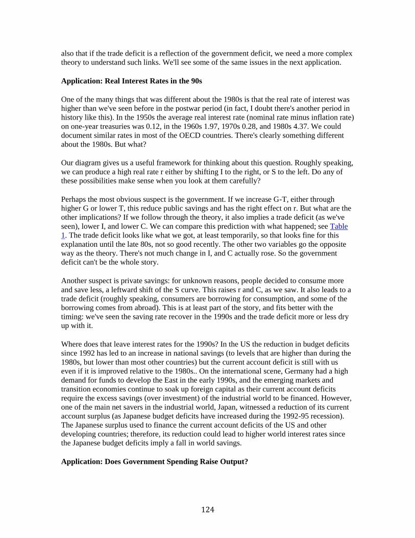
124

also that if the trade deficit is a reflection of the government deficit, we need a more complex

theory to understand such links. We'll see some of the same issues in the next application.

Application: Real Interest Rates in the 90s

One of the many things that was different about the 1980s is that the real rate of interest was

higher than we've seen before in the postwar period (in fact, I doubt there's another period in

history like this). In the 1950s the average real interest rate (nominal rate minus inflation rate)

on one-year treasuries was 0.12, in the 1960s 1.97, 1970s 0.28, and 1980s 4.37. We could

document similar rates in most of the OECD countries. There's clearly something different

about the 1980s. But what?

Our diagram gives us a useful framework for thinking about this question. Roughly speaking,

we can produce a high real rate r either by shifting I to the right, or S to the left. Do any of these possibilities make sense when you look at them carefully?

Perhaps the most obvious suspect is the government. If we increase G-T, either through

higher G or lower T, this reduce public savings and has the right effect on r. But what are the

other implications? If we follow through the theory, it also implies a trade deficit (as we've

seen), lower I, and lower C. We can compare this prediction with what happened; see Table

1. The trade deficit looks like what we got, at least temporarily, so that looks fine for this

explanation until the late 80s, not so good recently. The other two variables go the opposite

way as the theory. There's not much change in I, and C actually rose. So the government deficit can't be the whole story.

Another suspect is private savings: for unknown reasons, people decided to consume more

and save less, a leftward shift of the S curve. This raises r and C, as we saw. It also leads to a

trade deficit (roughly speaking, consumers are borrowing for consumption, and some of the

borrowing comes from abroad). This is at least part of the story, and fits better with the

timing: we've seen the saving rate recover in the 1990s and the trade deficit more or less dry up with it.

Where does that leave interest rates for the 1990s? In the US the reduction in budget deficits

since 1992 has led to an increase in national savings (to levels that are higher than during the

1980s, but lower than most other countries) but the current account deficit is still with us

even if it is improved relative to the 1980s.. On the international scene, Germany had a high

demand for funds to develop the East in the early 1990s, and the emerging markets and

transition economies continue to soak up foreign capital as their current account deficits

require the excess savings (over investment) of the industrial world to be financed. However,

one of the main net savers in the industrial world, Japan, witnessed a reduction of its current

account surplus (as Japanese budget deficits have increased during the 1992-95 recession).

The Japanese surplus used to finance the current account deficits of the US and other

developing countries; therefore, its reduction could lead to higher world interest rates since the Japanese budget deficits imply a fall in world savings.

Application: Does Government Spending Raise Output?

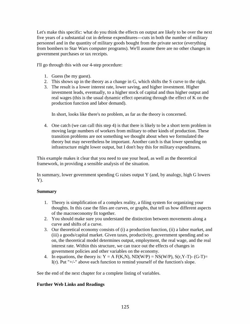
125

Let's make this specific: what do you think the effects on output are likely to be over the next

five years of a substantial cut in defense expenditures---cuts in both the number of military

personnel and in the quantity of military goods bought from the private sector (everything

from bombers to Star Wars computer programs). We'll assume there are no other changes in

government purchases or tax receipts.

I'll go through this with our 4-step procedure:

1. Guess (be my guest).

2. This shows up in the theory as a change in G, which shifts the S curve to the right.

3. The result is a lower interest rate, lower saving, and higher investment. Higher

investment leads, eventually, to a higher stock of capital and thus higher output and

real wages (this is the usual dynamic effect operating through the effect of K on the

production function and labor demand).

In short, looks like there's no problem, as far as the theory is concerned.

4. One catch (we can call this step 4) is that there is likely to be a short term problem in

moving large numbers of workers from military to other kinds of production. These

transition problems are not something we thought about when we formulated the

theory but may nevertheless be important. Another catch is that lower spending on infrastructure might lower output, but I don't buy this for military expenditures.

This example makes it clear that you need to use your head, as well as the theoretical

framework, in providing a sensible analysis of the situation.

In summary, lower government spending G raises output Y (and, by analogy, high G lowers

Y).

Summary

1. Theory is simplification of a complex reality, a filing system for organizing your

thoughts. In this case the files are curves, or graphs, that tell us how different aspects

of the macroeconomy fit together.

2. You should make sure you understand the distinction between movements along a

curve and shifts of a curve.

3. Our theoretical economy consists of (i) a production function, (ii) a labor market, and

(iii) a goods/capital market. Given taxes, productivity, government spending and so

on, the theoretical model determines output, employment, the real wage, and the real

interest rate. Within this structure, we can trace out the effects of changes in

government policies and other variables on the economy.

4. In equations, the theory is: Y = A F(K,N), ND(W/P) = NS(W/P), S(r,Y-T)- (G-T)= I(r). Put "+/-" above each function to remind yourself of the function's slope.

See the end of the next chapter for a complete listing of variables.

Further Web Links and Readings

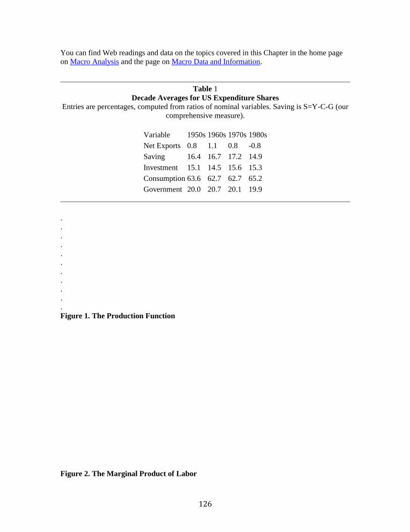
126

You can find Web readings and data on the topics covered in this Chapter in the home page

on Macro Analysis and the page on Macro Data and Information.

Table 1

Decade Averages for US Expenditure Shares Entries are percentages, computed from ratios of nominal variables. Saving is S=Y-C-G (our

comprehensive measure).

Variable 1950s 1960s 1970s 1980s

Net Exports 0.8 1.1 0.8 -0.8

Saving 16.4 16.7 17.2 14.9

Investment 15.1 14.5 15.6 15.3

Consumption 63.6 62.7 62.7 65.2

Government 20.0 20.7 20.1 19.9

.

.

.

.

.

.

.

.

.

.

.

Figure 1. The Production Function

Figure 2. The Marginal Product of Labor

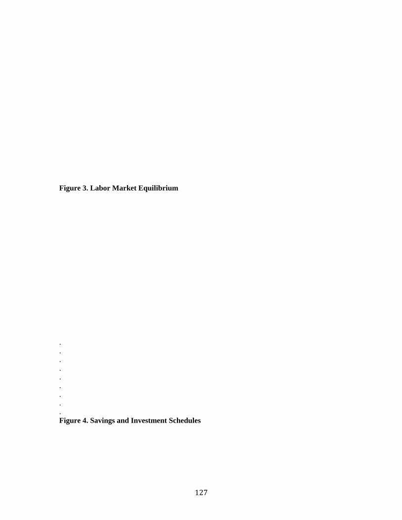
127

Figure 3. Labor Market Equilibrium

.

.

.

.

.

.

.

.

.

Figure 4. Savings and Investment Schedules

128

Figure 5. Short-Run Equilibrium (Effect of An Increase in G)

129

.

.

.

Figure 6. Long-Run Dynamics

130

Figure 7. High Real Interest Rates During an Economic Boom

131

Figure 8. Low Real Interest Rates during of a Recession

132

Figure 9. Determination of the Current Account

133

.

.

.

.

.

.

.

.

.

.

.

Figure 10. The Current Account Deficit in a Boom

134

Figure 11. The Current Account Surplus in a Recession

135

Copyright: Nouriel Roubini and David Backus, Stern School of Business, New York

University, 1998.

136

Chapter 6. Money and Inflation

Over the last few weeks we've seen how aggregate production possibilities (summarized in

the production function, the demand for labor, and the return on investment), consumers'

preferences (summarized by their willingness to work and save), and government policies

(spending and taxes) combine to influence the values of output, employment, wages, and the

rate of interest. All of these variables were "real": the relevant wage rate was the ratio of the

wage measured in dollars to the price of goods measured in dollars and the relevant interest

rate measured the rate of return adjusted for changes in the purchasing power of money. The

theory, thus far, has had nothing to say about "nominal" or "money" prices P, wages W, and

interest i.

Today we're going to look at the determination of nominal variables, specifically the price

level, its rate of change the inflation rate, and the nominal interest rate. The idea is that

inflation is associated with high rates of money growth. This theory, you'll see shortly,

exhibits a strong separation between real and nominal variables, since we have already

described how real variables are determined with no mention of the price level or inflation

rate. This is a hallmark of Classical theory. We'll see shortly that the Keynesian theory does

not have this feature, and economists differ about whether it is an embarrassment, a strength, or both.

The Quantity Theory of Money

Open Market Operations

Interest Rates and Inflation

Evidence

Application: Friedman's Money Growth Rule

Application: Big Inflations

Summary

Further Reading

Further Web Links and Readings Variable Definitions

The Quantity Theory of Money

We're going to start here with some pure reasoning that goes back a few hundred years. Like

a lot of good theory, it's based on an analogy. As a start, you should ask yourself what the

effect of a two-for-one stock split would be on the price of a stock. Suppose it's now selling

for 100, then you'd probably expect it to sell for 50 after a split, unless the split is an indicator

of some new information about the firm. As a first approximation we'll assume not. The point

is that the value of the firm's stock shouldn't depend on anything as arbitrary as the number of

shares outstanding: its value is more fundamental than that.

Now suppose we do the same thing with money. This is unrealistically simple (remember,

we're doing theory now!) but suppose the government were to replace every dollar with two

new dollars, marked so we can tell the difference between old and new dollars. Then you'd

expect, I think, that prices in terms of new dollars would be twice as high. In short, changes

in the money supply executed in this way will be associated with proportionate changes in prices, with no effect on output or employment.

137

Of course the world is more complicated than this, and monetary policy consists of more than

just currency exchanges, but some of the same reasoning applies more generally (or may

apply, we'll look at some data shortly). The so-called quantity theory of money is the result of

two ideas: that money is not fundamental (pieces of paper don't change the effectiveness of

GM's manufacturing processes or marketing strategies), and that its usefulness is in executing

transactions. Let's start with the latter. Suppose we think of Y as all the transactions in the

economy and PY is the dollar value of all these transactions (sales revenue). Then we need M dollars of money to make all these transactions each period, or

M = P Y.

Note that this equation has the stock-split property: if we double M then we double PY. We

can make this more specific by associating transactions Y with real GDP, PY with nominal

GDP, and P with the GDP deflator.

A slight generalization is that money can be used several times each period for transactions,

as it goes from one person to another. That is,

M V = P Y,

where V is the velocity of money, the number of times each period a unit of money is in a

transaction. The assumption of the quantity theory, which dates back at least three hundred

years (a long time in economics), is that velocity is approximately constant. This equation

maintains the stock-split property, that increases in M are associated with proportionate increases in PY.

In principle the increase in PY could be in P, Y, or both. Later we'll consider a theory in

which Y changes are possible (the Keynesian theory). But for now let's say that Y is not

affected by M. This is the assumption that fundamentals like Y are not influenced by M, just

as a firm's value is not influenced by a stock split. The theory behind this in our case is that Y

has been determined by the production function and the labor market. That leaves only one

thing to adjust when M changes: the price level P. In short, changes in the stock of money lead, in this theory, to proportionate changes in prices.

The same theory can be reinterpreted in terms of the inflation rate, the rate of growth of the

price level. To see this, we need to covert the quantity theory relation to growth rates. We take the quantity equation at two different dates and divide, getting

(Mt /Mt-1) (Vt /Vt-1) = (Pt /Pt-1) (Yt /Yt-1 ).

For reasons similar to our growth accounting relations in Chapter 4, this leads to (approximately)

(Mt -Mt-1)/Mt-1 + (Vt -Vt-1)/Vt-1 = (Pt -Pt-1 )/Pt-1 + (Yt -Yt-1)/Yt-1

or:

m + v = p + y

138

where lower case characters represent the rate of growth of upper case variables (i.e, m is the

rate of growth of money M).

If velocity is constant we get, approximately, the growth rate of money equals the growth rate of prices (inflation) plus the growth rate of output

(Mt -Mt-1)/Mt-1 = (Pt -Pt-1)/Pt-1 + (Yt -Yt-1)/Yt-1

or:

m = p + y

If money growth does not influence output, then higher money growth leads to higher

inflation. Period. This prediction is overly strong, as we'll see, but the simplicity has some

value of its own, including making it easy to remember. As Milton Friedman put it: "Inflation

is always and everywhere a monetary phenomena." It's only after you think about that

sentence for a while that you realize it's not as informative as it first sounds.

Open Market Operations

We'll go into this in greater depth later on, but for now let me give a quick overview of how

governments get money into the system. One way, as we've seen, is to print money to finance

government deficits. If we measure the deficit in dollars (rather than the base-year prices we

generally use in the National Income and Product Accounts) this is something like:

Pt (Gt-Tt) = dMt = Mt - Mt-1

which says each dollar of deficit is financed by printing dM new dollar bills. Literally, the

government pays its bills with currency. This is how Yugoslavia, for example, got such a

high inflation rate: the costs of fighting the war were paid for, in large part, with cash, which by now is nearly worthless.

The other way the government gets currency into the economy is by changing the

composition of its balance sheet. The government's balance sheet might be represented, in

highly streamlined form, as (approximate numbers for 1992, billions of dollars):

Government Debt 3,000

Bonds 2,850

Currency 150

The government also has some assets, but let's ignore these for the moment. The government

thus has a "capital structure,'' to use some finance jargon, of about 97 percent interest-bearing

debt and 3 percent currency, which pays no interest.

Now suppose the government (generally the central bank) wants to increase the quantity of

currency in the economy by 10 billion dollars. It does this by buying 10 billion of bonds from

someone in the private sector, and paying for them in cash. This changes the balance sheet

139

accordingly. This is referred to as an open market purchase of government securities, for

obvious reasons, and is the method of choice in most developed countries. The institutional

details sometimes looks quite different (the US, for example, has a highly developed "money''

market for short term securities, and we never actually see cash changing hands), but this is still basically what is going on underneath it all.

Interest Rates and Inflation

We've seen that the real rate of interest is the difference between expected inflation and the

nominal rate of interest that we see quoted in the paper, or in letters,

it = rt + pte.

The question is what our theory tells us about the relation to be between inflation and

nominal interest rates. The theory that fits in with our stock-split analogy (fundamentals do

not change, and r is a fundamental) is that the real interest rate r is determined by investment

and saving without regard for money and inflation. That's apparently what we assumed in our

presentation of this aspect of the Classical theory, since there was no mention of money when

we determined the real interest rate and output. For a given real interest rate, what happens to

the nominal interest rate if inflation rises? Clearly the nominal interest rate rises by the same

amount. Thus an increase in inflation (really, expected inflation since it's the future that matters) leads to higher nominal interest rates.

Evidence

Quick review. Real output Y and the real interest rate r are determined by the real side of the

economy: the production function, the labor market, and the capital market. The money stock

governs the price level and the rate of inflation. In conjunction with the real side of our

theoretical economy, the quantity theory states that higher money growth is associated with

higher inflation and nominal interest rates. This complete separation between real variables

and inflation is overly strong, esp in the short run, but it illustrates what I think are the

important long-run effects. But don't take my word for it, let's look at some data.

Here's how the theory does in practice. The first prediction can be expressed two ways:

velocity is approximately constant or (this follows from the quantity equation) the price level mimics the money stock adjusted for output growth. In logarithms,

log Pt = log Mt - log Yt + log Vt.

By assumption V is constant, so if M is growing faster than Y we should see a comparable

rise in the price level. Do we? I've graphed these variables in Figure 1, with M defined as the

broad money stock, M2 (which includes, as we've noted, time and saving deposits as well as

checking accounts). (Y here is real GDP and P is the implicit GDP deflator.) I think you'll

agree that the relation is pretty good---maybe as good as you'll ever see in economics (we

have aspirations, but this isn't physics). To a first approximation, it seems that the assumption

of constant velocity isn't too bad. Most of the increase in the price level over the past thirty

years has been associated with a comparable increase in the broad stock of money. There are,

140

however, some wiggles in velocity over the short term (up to three years, say) that we may

want to look more closely at.

How well does this work in the short run? You can see in Figure 1 that there are some

"wiggles" that reflect fluctuations in velocity. What does that do to our prediction? If we

graph annual growth rates we know (recall our GDP graphs) that these short-run movements

will show up more clearly. In terms of the theory, the prediction is

(Pt -Pt-1)/Pt-1 = (Mt -Mt-1)/Mt-1 - (Yt -Yt-1 )/Yt-1

or:

p = m - y

since velocity is assumed to be constant. These variables are graphed in Figure 2, where we

see that the connection between money growth and inflation is much looser for these short-

run movements. In this sense, the theory is a much better prediction of long-run tendencies than short-run fluctuations.

Our second prediction concerns interest rates. In the theory we saw that the real interest rate

was determined by saving and investment schedules. In principle these curves, and hence the

real rate of interest, can move around over time---for example, as government deficits vary.

The nominal interest rate will move around for a second reason: because expected rates of

inflation vary. With the exception of the Korean War, inflation was less than four percent

until the late 60s. It rose during the Vietnam War, peaked above 10 percent in 1975, declined

slightly, and peaked again at about ten percent in 1980. The question for the moment is

whether this pattern is reflected in interest rates. In Figure 3 I've graphed the one-year

treasury rate and the rate of inflation (computed from the GDP deflator). Here, too, the

relation isn't bad: we tend to see high rates of interest in those periods when inflation is

highest, and vice versa. As a rough approximation, at least, nominal interest rates reflect rates

of inflation. There are still, though, some significant short-run deviations. Note in particular

that real rates, measured as the difference between the two curves, were higher in the late 1980s than elsewhere in the entire postwar period.

Thus the classical quantity theory seems to provide a reasonably good guide to long-run

trends in inflation and interest rates. In the short-run, though, something more complicated

seems to be going on. That's our objective for the Keynesian theory to come: to get a better

understanding of these short-term fluctuations.

Application: Friedman's Money Growth Rule

The quantity theory was the basis (or a big part of it) for one of the sharpest policy debates in

the postwar period. Then, as now, there were many businessmen, economists, and

government officials who thought that monetary policy should be chosen to micro-manage or

fine tune the economy: to help smooth out the recurrent ups and downs that we've labeled the

business cycle. Milton Friedman, who made a career out of playing devil's advocate,

advocated precisely the opposite: that the Federal Reserve should follow a policy consistent

with (we'll leave the operational aspects for later) a constant rate of money growth of about 4

141

percent a year. Given output growth of about three percent, on average, that would be

expected to lead to average inflation of about 1 percent a year.

Over the years Friedman provided many arguments for constant money growth rates. Here

are a few of them (stated as hypotheses to think about, not self-evident truths):

This policy should have good long-run properties (low inflation).

It might be better than actual policy over the last forty years, since it would probably

eliminate some of the big mistakes (like the high inflation rates of the 1970s).

Discretionary short-run policy management leads, in practice, to shortsightedness and

bad long-run policy decisions. Eg, suppose the Fed continually increases the money

stock to avoid recessions. The result is higher inflation, not demonstrably better

output performance.

Monetary policy is a string, you can pull on it but you can't push. In other words, you can use it to start a recession, but not to stop one.

The main counterargument is that you may be able to do better than this: why tie your hands

behind your back?

Friedman's points are a combination of theory, fact, and pessimism regarding government,

little of which is inarguable. But I think all of these issues are important. It's still an open

question how well (or poorly) such a policy would do, but it's had an effect on actual policy. I

think that after the experience of the 1970s, when policy repeatedly failed to eliminate either

inflation or business cycles, policymakers are less ambitious now about managing the

economy in the short-term. Greenspan, for example, does not adhere to a rigid money growth

rate rule, but he uses monetary growth rates as guides to the long-run inflation content of his

policies. At the same time, he is willing to make large policy changes in response to special

conditions, something clearly opposed by Friedman. In the wake of the 1987 stock market

crash Greenspan, in conjunction with other central bankers, engineered a sharp increase in

funds and a sharp drop in interest rates to cushion the fall. There was some worry at the time

that this would eventually lead to higher inflation, and inflation did rise somewhat over the

next 3-4 years, but I think most observers view it as an astute move that may have prevented financial and economic disaster.

There's also some discussion recently about whether monetary policy should be more

expansionary. The argument in favor is that this might help us get out of a recession when we

are stuck in one; we'll see how next week. Friedman's counterargument might be that (i) it

won't do it ("string") and (ii) it will lead to inflation over the longer run. The Fed currently

has members with both views, plus the entire spectrum in between. And since you never

know what would have happened if you had followed some other policy, there's lots of room for differences of opinion.

My feeling is that, like much of what Friedman says, there's a useful point here but he's

pushed it too far. I'd guess that a constant growth rate rule, for average growth rates over two

to five years, would be a pretty good long-run policy. That leaves room for short term

deviations, without letting them get out of hand: so when the economy is headed towards a

recession, the Fed will expand the money supply and reduce interest rates; while it will do the

reverse if the economy is growing too fast and there are signals of inflationary pressures in

142

the economy. This would probably eliminate most of the excesses of the last thirty years. As

an economist at the Bank of Canada put it: "Our goal is to avoid disasters, like the inflation of the 1970s. Anything else is a bonus."

Application: Big Inflations

In the 1980s, Argentina, Bolivia, Brazil, and Israel have experienced very large inflation

rates, all over one hundred percent a year and some over a thousand. We can confidently

expect several more cases of large inflation over the next decade.

But why? If the relation between money growth and inflation is so clear, why don't these

countries simply print less money? If only it were so easy! The real problem most of these

countries had was a large fiscal deficit. Let's think how that influences monetary policy. If a

government is running a deficit, then it must issue iou's of some sort to pay for it. Roughly,

speaking, it may issue money (dollar bills or their local equivalent) or interest-bearing debt (treasury bills and notes) denoted with the variable B. Mathematically we can express this as

Pt (Gt - Tt) = dMt + dBt,

or, in real terms:

Gt - Tt = dMt / Pt + dBt / Pt

where the two terms on the right are issues of new money (dM) and new interest-bearing debt

(dB), respectively. This is an example of a government budget constraint: it tells us that what

the government doesn't pay for with tax revenues, it must finance by issuing debt of some

sort.

So why do these countries increase the money supply? The problem, typically, is that a

political impasse makes it nearly impossible to reduce the budget deficit. Given the

government's budget constraint, it must then issue debt. Now for US debt there is apparently

no shortage of ready buyers, but the same can't be said for Argentina or Russia. If they can't

issue debt and they can't reduce the deficit, the only alternative left is to print money: in

short, when they can't pay their bills any other way, they pay them with money, which is easy

enough to print. The effect of this, of course, is that these countries experience extremely high rates of inflation.

Note that whenever a central bank prints "fresh money" it can obtain goods and services in

exchange for these new pieces of paper. The amount of goods and services that the

government obtains by printing money in a given period is called "seignorage". In real terms, this quantity of goods and service is given by the following expression:

Seignoraget = dMt / Pt = New bills printed during the period / Price level during the period.

The monetary aggregate that the central banks control directly is the "monetary base",

consisting of currency in the hands of the public and reserves of the commercial banks

deposited in the central bank. Thus, when we refer to a central bank as "printing more money", we mean increasing the monetary base.

143

Note that since the government, by printing money, acquires real goods and services,

seignorage is is effectively a tax imposed by the government on private agents. Such a

seignorage tax is also called the inflation tax. The reason is the following. From the definition

of seignorage:

Seignoraget = dMt / Pt = (dMt / Mt ) (Mt/Pt)

Since the rate of growth of money (dM/M=m) is equal to inflation (p) (assuming, for

simplicity, that the rate of growth of output 'y' is zero), we get:

Seignoraget = pt (Mt/Pt)

In other terms the inflation tax is equal to the inflation rate times the real money balances

held by private agents. This makes sense: the inflation tax must be equal the tax rate on the

asset that is taxed times the tax base. In the case of the inflation tax, the tax base are the real

money balances while the tax rate at which they are taxed is the inflation rate. In other terms,

if I hold for one period an amount of real balances equal to Mt/Pt, the real value of such

balances (their purchasing power in terms of goods) will be reduced by an amount equal to pt

(Mt /Pt) after one period. The reduction in the real value of my monetary balances caused by

inflation is exactly the inflation tax, the amount of real resources that the government extracts from me by printing new money and generating inflation.

To understand the relation between money creation, budget deficits and seignorage see, for

example, the data for Brazil in Figure 4, Figure 5 and Figure 6. Through 1993 it appeared that

Brazil was committing the cardinal sin of inflation stabilization: they are trying to reduce the

inflation rate by controlling money, but without solving their underlying budget problems.

Experience indicates that this approach is bound to fail.

The thing I like about this analysis is that it gives a strange twist to Friedman's quote:

inflation might be a monetary phenomenon, but the money is a reflection of bad fiscal policy,

not monetary policy. We might say instead: "Inflation is always and everywhere a fiscal

phenomenon."

To understand better why inflation is a fiscal phenomenon, note again that a government

with a budget deficit can finance it either by printing money (that leads to seignorage or the inflation tax) or by issuing public debt:

(G-T) = dM/P + dB/P = p (M/P) + dB/P

Note also that countries such as Argentina, Bolivia, Brazil and Israel had very high inflation

rates in the 1980s. Now, if inflation was purely a monetary phenomenon caused in the first

place by an exogenous excessive rate of growth of money, these countries could have

reduced inflation quite fast by printing less money and reducing the growth rate of the money

supply. Instead, all these countries had a really hard time in reducing their inflation rates. So,

if inflation was due to an exogenous high growth rate of money, why didn't these countries

print less money ? The main problem is that these countries had large structural budget

deficits and printed money to finance it. In this sense, the excessive growth rate of money

144

that led to seignorage and caused inflation was not exogenous but rather endogenous and

caused itself by the need of these governments to finance their budget deficits.

Note, however, that these countries could have in principle avoided the high inflation if they

had cut their budget deficits (thus reducing the need for seignorage revenues) and/or if they

had financed their budget deficits by issuing bonds rather than by printing money. This leads

to the further question: why weren't the deficits reduced and/or why weren't the deficits financed by issuing bonds?

Budget deficits are often very hard to reduce for political and structural reasons: cutting

deficits implies reducing government spending and/or increasing taxes and both policies are

politically unpopular. Also, in countries with inefficient tax collection systems and where

there is a lot of tax evasion, it is hard in the short-run to reform the tax system so as to

increase (non-seignorage) revenues. Conversely, increasing seignorage revenues is much

easier as it implies printing new money, an executive action rather than a legislative action as

in the case of traditional taxes. Of course, seignorage is as much of a tax as regular taxes but

it is politically more hidden (at least at low levels of inflation) as the effect of higher money growth leads to higher inflation only slowly over time.

For what concerns the possibility of (non-inflationary) bond financing rather than

(inflationary) monetary financing of the deficits, there are several obstacles to such a policy

option in many developing countries. First, bond markets are not very well developed (and in

some cases altogether absent) in many countries. Second, citizens are concerned about

buying nominal long-term bonds issued by the domestic government because an unexpected

increase in inflation by the government would lead to a fall in the real value of these bonds

(that is equal to a wealth tax on the public holdings of such bonds). Third, bonds indexed to

inflation and/or short-term bonds that pay returns close to current market rates are still

subject to default risk if the government decide to renege on its obligations. Fourth, the

ability to borrow abroad and/or issue bonds denominated in foreign currency in international

capital markets may also be limited by the default risk of the country. Fifth, even when some

bond borrowing may be available either domestically or abroad, governments may not be

willing to issue such bonds. In fact, bond financing is more expensive than monetary

financing (seignorage) since governments do not pay interest on their monetary liabilities

while they have to pay interest (high ones if inflation is high) on their borrowing. Sixth,

borrowing by issuing debt means that the stock of debt goes up every year by the amount of

the the flow of debt financing: Bt+1 = Bt + dBt. This growth of debt may be very costly and

not be sustainable in the long-run. In fact, if the public debt grows a lot (relative to GDP), at

some point private agents might become unwilling to buy new debt (or even roll-over old

debt that comes to maturity) as high debt increases the probability that the government might

at some point default on its debt obligations. So, if such a panic occurs and the private sector

refuses to buy new debt and/or renew the old one, a government with a structural budget

deficit will eventually be forced to start printing money and thus create inflation. Therefore,

in face of a structural deficit, trying to reduce inflation today by issuing bonds rather than

printing money will just lead to higher debt in the future that will eventually force the

government to monetize the deficit (when the debt constraint is hit) and thus will cause

inflation in the future. Again, inflation is a fiscal phenomenon and there is no escape from it

if the underlying deficit problem is not solved: attempts to reduce current inflation by issuing

145

bonds only implies that future inflation will be higher when the ability to issue debt is

exhausted and the government is forced to switch to a monetary financing of the deficit.

Therefore, while the near proximate cause of high inflation is always monetary as inflation

is associated with high rates of growth of money, the true structural cause of persistent high

inflation is a fiscal deficit that is not eliminated with cuts in spending and/or increases in

(non-seignorage) taxes.

Finally, note that for someone operating an international business, the thing to remember is

that "big inflations'' are relatively common. So what do you do if you're hit with one? You'll

probably find that the most important thing you can do is streamline your cash management.

If you can reduce the payment terms from (say) 60 days to 30 days, you increase your "real''

revenue substantially. You may also find that big inflations leads to policy changes, like price

controls, that make your life more complicated. Finally, you may find that your financial

statements, and incentive programs based on them, are highly misleading, since they measure

performance in terms of the local currency, whose value is changing rapidly. For a US

subsidiary, high inflation triggers a change in the rules for translating financial entries into

dollars for tax and reporting purposes (hyperinflation is defined, for this purpose, as 100

percent over 3 years).

Summary

1. The Classical theory exhibits complete separation between real variables and

inflation. There is, by construction, no effect of money growth on real output or the

real rate of interest.

2. In the Classical theory, inflation is driven by money growth (the quantity theory) and

nominal interest rates by inflation (the Fisher relation).

3. In the data, the theory's predictions look better for long-run trends than for short-run

fluctuations.

4. Extremely high rates of inflation are generally associated with high rates of money

growth, often the result of financing large fiscal deficits by printing money. In this sense, there's no simple distinction between monetary and fiscal policy.

Further Reading

Rukstad's "Colgate-Palmolive in Mexico" (Harvard Case 9-389-105, reprinted in Michael

Rukstad, Corporate Decision Making, Dryden, 1992) is a terrific example of a US subsidiary

operating in a high inflation environment (Mexico in the mid-1980s). Choi and Mueller's

International Accounting (Prentice-Hall, 1992) contains nice reviews, with examples, of

accounting issues related to currency translation (ch 4) and high inflation (ch 5) (which we'll

see shortly are closely related).

Further Web Links and Readings

For more Web readings on this chapter's topics look at the home pages on Macro Analysis

and Macro Data sources and the controversies on NAIRU and the New Economy.

Variable Definitions

146

A = (total factor) productivity

Def = G - T = government deficit

G = government purchases of goods and services

i = rate of interest in dollars ("nominal")

I = investment (purchases of new capital goods)

K = stock of physical capital (number of machines, factories, etc)

M = stock of money (number of dollars outstanding)

MPN = marginal product of labor

N = employment (ND = labor demand, NS = labor supply)

NX = net exports = exports - imports

NFA = net foreign assets = foreign assets - foreign liabilities

i x NFA = net income payments from abroad

CA = NX + i x NFA = current account

P = price of goods in dollars (aka price level)

pe = expected inflation rate

r = "real" rate of interest = i - pe

S = Y-C-G = national savings

T = taxes net of transfer payments and other government cashflow not included in G

V = velocity = PY/M

W = wage rate in dollars

W/P = "real" wage rate

Y = "real" GDP = output = income

Y* = "real" GNP = GDP + i x NFA

147

148

149

150

151

152

Copyright: Nouriel Roubini and David Backus, Stern School of Business, New York

University, 1998.

153

Chapter 7. Foreign Exchange Rates

We turn now to a more detailed look at exchange rates, with the simple message that real

exchange rates are highly variable. Examples include Mexico in 1981-82, when the peso

collapsed, the real appreciation of US$ in the 1980s and the Japanese autos in early 1993,

when the yen rose sharply.

Classical Theory of Exchange Rates

Fixed Exchange Rate Regimes: Mexico 1982

Exchange Rates in the Short Run

Application: US - Japanese Auto Makers Competition and the Dollar in the 1980s

Application: Toyota, 1991-93

Summary

Further Reading Further Web Links and Readings

Classical Theory of Exchange Rates

The Classical theory of exchange rates is basically the quantity theory of money and the

theory of purchasing power parity, or PPP, which we looked at in Chapter 3 of these lectures.

The first ingredient is the quantity theory, which tells us that prices of goods reflect stocks of

money:

P = MV/Y

Pf = Mf Vf /Yf .

With V's fixed (the premise of the quantity theory) and ignoring Y's (just to make things

easier), we see that price increases are caused by increases in money M. We saw in Chapter 6 that this is a reasonable approximation over periods of several years or more.

The second ingredient of our theory is PPP, which I'll review quickly. Let us say that the

price of US goods, measured in dollars, is P, and the price of foreign goods, measured in

foreign currency units, is Pf (f for foreign), and the spot exchange rate, measured as the dollar

price of one unit of foreign currency, is S. Then the dollar price of foreign goods is SP. The

logic behind PPP is that prices of comparable goods should not be different in two locations, so we should see (at least approximately)

P = S Pf .

or

S = P / Pf (1)

A minor variant of this is

RER = S Pf /P = 1;

154

ie, the real exchange rate is constant if the PPP holds. Equation (1) in growth rates is

(St - St-1)/St-1 = (Pt -Pt-1)/Pt-1 - (Pft - Pf

t-1)/Pft-1 ,

so that the rate of depreciation of the currency is equal to the difference between the two countries inflation rates. We'll look at this relation in the data shortly.

Putting the two ingredients together, we get

S = (M/Mf ) (V/Vf ) (Yf /Y). (2)

Roughly speaking, we see that our currency weakens (S rises) if we issue more money than the other country (M rises more than Mf).

There's no question that both ingredients are poor descriptions of reality over short time

periods of time. What may surprise you is that they do considerably better over longer

periods. Figure 1 illustrates the first ingredient, the relation between exchange rate changes

and differences in inflation rates. The figure reports average annual growth rates for several

countries for the period 1970-90. The theory says they should be the same, and in fact they're

pretty close: countries with high inflation rates also experienced the greatest depreciation of

their currencies. In Figure 2 we turn to the relation between depreciation and money growth.

Applying our old trick with logarithms to (2), we see that changes in the exchange rate are approximately equal to differences in money growth rates:

(St - St-1)/St-1 = (Mt - Mt-1)/Mt-1 - (Mft - Mf

t-1)/Mft-1 .

The approximation is based on two things: that velocities are constant, and that differences in

output growth across countries are small (so we don't miss much by ignoring them, even

though in principle they should be there). We see in Figure 2 that this is pretty good, too, for

averages over the same twenty-year period.

Fixed Exchange Rate Regimes: Mexico 1982

The story behind PPP is that exchange rates should eventually lead to comparable prices of

goods in different countries. If goods are more expensive in Germany than the US, a fall in

the value of the DM will bring them back into line. The evidence is that this tendency asserts

itself eventually.

When the exchange rate is fixed by government decree, as it is in many countries around the

world, this mechanism operates a little differently. We're going to look at the collapse of the

Mexican peso in 1982 as an example of what can happen. The short story is that the peso

collapsed in 1982. Between early 1977 and early 1980, the peso traded in the neighborhood

of 23 pesos per dollar, a level enforced by the Banco de Mexico, the Mexican central bank.

We'll return shortly to how they did this. Through January of 1982, the rate crept up, hitting

26.6 the end of the month. On February 5, President Lopez-Portillo announced that the

central bank would defend the peso "like a dog," presumably to assure financial markets that

the government would not let the peso collapse. On February 19 this effort was abandoned,

and the peso immediately fell 29 percent against the dollar, reaching 45 pesos to the dollar by

155

the end of the month. The peso continued to fall throughout the decade, and now trades at

about 3000 to the dollar. The complete history of the peso for this period is illustrated in Figure 3.

So what happened?

Fundamentals. There are several dimensions to this question, but the most obvious one is that

Mexico's fixed exchange rate was inconsistent with its other policies. You can see in Figure 4

that while Mexico attempted to fix its currency, its monetary policy led to much more rapid

growth in its stock of money than in the US. This is illustrated by the "dash-dot" line in the

figure, denoting the ratio of the money stock in Mexico to that in the US. As a result, prices

in Mexico rose more rapidly than those in the US, with Mexico averaging between 20 and 30

percent inflation between 1979 and 1981. The dashed line in Figure 4 depicts the sharp rise in

the ratio of Mexican prices to American. By the end of 1981, prices had risen substantially

more in Mexico than the US, leading many Mexicans to shift their spending and investments

outside the country. By February 1982, the discrepancy in prices proved to be indefensible,

and the peso imploded. In short, the enormous departure from PPP was too much for the

system to withstand, so the exchange rate collapsed. You can see in the figure that the decline

in the peso brought prices back into line with PPP (for a while).

Fixing the Exchange Rate. Another dimension to our question is the central bank's behavior.

You might think that the central bank can simply announce an exchange rate, but a little

thought will tell you it's not so easy. To take a slightly frivolous example, I could claim that

my apartment is worth 2 million dollars, but if no one is willing to buy it for that price it's not

clear that the statement means anything. For related reasons, the central bank must back up its claim to fix the exchange rate.

In the simplest version of a fixed exchange rate, the central bank supports the price by buying

and selling as much foreign currency as people want at the set price. If people want dollars,

the bank supplies dollars, if they want pesos, the bank supplies pesos. As with monetary

policy, the central bank does this by changing the composition of its balance sheet. The

Banco de Mexico might have had a balance sheet something like this in late 1981:

Assets

Liabilities

FX Reserves 5 Monetary Base 100

Other 115 Bonds 20

We could do this in any units we like, but let's say the units are billions of US dollars. The

numbers (which I made up) reflect the fact that there is not much of a government bond

market in Mexico---it's primarily a captive market of banks, who are required to hold

government securities. The 5 under "FX Reserves" is holdings of dollar-denominated assets

(largely US government securities). If people want to buy, say, 2 billion more US dollars, this

would show up as a decline of 2 billion in FX reserves and a corresponding decline in the monetary base (Mexican currency), as people trade in their pesos for dollars.

156

The Banco had some trouble backing up the exchange rate policy in February 1982, when a

run on the peso depleted almost half of its reserves (see Figure 5). If they ran out of reserves,

of course, they would be unable to deliver on their pledge to meet market demand at the

current price. They compromised by letting the peso fall, which relieved some of the pressure

for a time. In August of 1982, renewed pressure on the peso lowered reserves further. This

time the bank outlawed many fx transactions, thereby taking the exchange rate out of the

hands of the market. As the jargon would have it, the peso was no longer "convertible" into

foreign currency without explicit permission from the central bank. In that sense, the official

price was like the 2m claim for my apartment: virtually meaningless, since you could not

generally buy or sell at that price. Those with permission were able to buy dollars cheaply,

while others paid a much higher prices in the parallel or black market. These exchange

controls caused serious problems for both Mexican business and foreign businesses operating

in Mexico, since without foreign currency they could not import foreign goods. And since

foreign investors could not be assured of repatriating their earnings, many avoided investing

in the first place. Many Mexicans, in fact, got their own assets out of the country ahead of

time, sparked by their fear (subsequently borne out) that currency controls would make it impossible to do later.

To summarize: el Banco tried to set the exchange rate at a level that was wildly inconsistent

with its fundamental PPP value. When this didn't work, they let the peso fall and limited fx transactions.

Lessons. This series of events is (perhaps surprisingly) relatively common, and suggests some

lessons for businesses operating in foreign countries.

1. Fixed exchange rates aren't fixed forever. They simply substitute infrequent large

movements for more frequent smaller movements. If you get caught, they can kill you.

Anyone holding pesos on February 19, 1982, lost 29 percent of their dollar-equivalent value in a day, and more after that.

2. Operate in hard currencies when you can. One strategy for dealing with such risk is to do

business in dollars, or some other hard currency. US banks, for example, denominated their

loans in dollars, so the collapse in the peso did not hurt them on its own. But the collapse of

the economy that went with the fall in the peso did hurt them, with the result that most loans

were repaid only in part. Mexicans, too, tried to switch to dollars, but government restrictions made this difficult to do on a large scale.

3. Enter after the fall. A colleague of George Soros's said once that the best opportunities

come when situations change from "disaster" to "bad". Anyone entering the Mexican market

in 1982 or 1983 had, at least, the advantage of buying low. With Spring break coming up, you might use the corollary: the cheapest vacations are right after the currency collapses.

Exchange Rates in the Short Run

Although the theory of PPP works moderately well for long periods of time (decades?), it is a

relatively poor description of shorter term movements. An example of such evidence, similar

to that for Mexico, is Figure 6, where we see real exchange rates for the US vs Germany,

157

Japan, and Mexico. In the theory of PPP [equation (1)] this should be constant. In the data, it

is not.

For Germany we see that the exchange rate is flat until the early 1970s, as a result of the

Bretton Woods fixed exchange rate system in place at the time and the small differences in

inflation between Germany and the US in the 1960s. But with the collapse of the Bretton

Woods system, the DM rose and prices of German goods rose with them. The log scale of the

figure tells us that German goods rose about 40 percent relative to American goods between

the beginning of 1971 and the end of 1973. The 1973-93 period is remarkable for enormous

fluctuations in both directions, with a sharp fall in the DM in 1980 and a sharp rise in 1985 as highlights.

The graph for Japan tells us that Japanese goods have gotten progressively more expensive

than US goods over the last thirty years, although again there have been significant ups and

downs along the way (and note that the scale is larger than that for Germany). One issue that

comes to mind is the Japanese trade surplus. Although this has some connection with the

exchange rate, the graph tells us that the rising surplus has occurred while prices of Japanese

goods have risen, on average, when most people think the connection should go the other

way. The Clinton Administration, for example, talked up the yen in 1993 and again in early

1995 in the hope that it would bring the Japanese surplus down and reduce the US trade deficit.

Mexico exhibits a boom/bust pattern common among developing countries, with gradual

rises in the real exchange rate reversed periodically by sudden collapses in the peso---note the sharp drop in 1976, as well as the collapse in 1982 that we've already examined.

Academics love to quibble about these things (and, to be fair, our quibbling is useful for

separating useful statistics from misleading ones), and some of them have suggested that the

problem may be that the goods in the CPI's are not comparable. You'll recall that the basis of

the theory is arbitrage: if a good is cheaper in one place than another, people will buy more of

it and drive its price up until the difference disappears. In fact, we see just that with gold:

there is very little difference between the prices of gold in the US, Japan, or Germany. The

same is true for some agricultural commodities, but barriers to trade that inhibit arbitrage

allow higher prices of sugar in the US and rice in Japan. In general. prices even of

comparable goods vary widely internationally. In short, the theory of PPP is a poor theory for

the short run. We see enormous fluctuations in real exchange rates, meaning that prices of

goods vary widely across countries. Anyone who has visited Japan in the recent past can vouch for that.

What are the reasons for the breakdown of the PPP in the short-run ? There are a number of reasons for the failure of PPP:

1. The CPI of different countries are not comparable since they include very different goods.

2. The CPI includes many goods that are not traded (such as services); the PPP will not hold

for these goods. For example, a haircut in Bombay might be cheaper than in New York but few New Yorkers would fly to Bombay just to get an haircut.

158

3. PPP (or the Law of One Price, LOP) holds better for homogenous commodities that are

traded internationally (gold, oil, agricultural commodities, raw materials). In these well developed commodity markets, the goods arbitrage implied by the PPP holds very fast.

4. Even for homogenous goods, the PPP might hold very well: by and large, prices even of

comparable goods vary widely internationally. The Economist (see the article "McCurrencies:

where is the beef?" also available in the Reading package) runs a feature on the prices of Big

Macs around the world that makes the same point. The Big Mac is a good example, because

McDonald's makes sure that the product is the same everywhere. Yet we see that its price is

not the same. [In this reading, the last column, labeled over/under valuation, is the percent

deviation of the German real exchange rate from one, with the sign reversed. Thus the +37

for Germany means that Big Macs are 37 percent more expensive in Germany than the US.]

5. If firms can "price discriminate" between domestic and foreign markets, PPP (or Law of

One Price) will not hold for homogenous goods. The price of German (Japanese) cars is very

different in the US relative to Germany (Japan). Price discrimination is feasible only under some conditions.

6. Finaly, if goods are not homogenous (Japanese cars are not the same cars as US cars), the

US price in dollars of Japanese cars does not have to be equal to the price in dollars of US

cars. Moreover, changes in the nominal exchange rates will affect the relative price of

Japanese versus US cars in complex ways that we discuss in the next section.

US - Japanese Auto Makers Competition and the Dollar in the 1980s

We will discuss the role of exchange rate in the competition between US and Japanese car

makers in the 1980s. To undestand the importance of exchange rate note that the dollar had a

dramatic appreciation between 1980 and 1985 and a major depreciation from 1985 to 1989. Specifically:

Exchange Rates:

1980:

SY/$ = Yen/Dollars = 200

S$/Y = Dollars/Yen = 0.005

1984:

SY/$ = Yen/Dollars = 250

S$/Y = Dollars/Yen = 0.004

1989:

SY/$ = Yen/Dollars = 139

159

S$/Y = Dollars/Yen = 0.0072

The data above show that the $ appreciated relative to the Yen by 20% between 1980 and 1984; and depreciated relative to the Yen by 44% between 1984 and 1989.

Let us consider now the effects of exchange rate on the pricing policies of domestic (US) and foreign (Japanese) car makers.

Consider the competition in the car industry in 1980. Let us suppose that the prices of American and Japanese cars in 1980s were:

Price of a U.S. car in the U.S. in Dollars (P$): $10,000.

Price of a Japanese car in Japan in Yen (PyJ): 2 million Yen

These numbers are not exact but are used here for the sake of the excercize.

Since the price of a good is equal to the cost of production times the gross profit margin (mark-up rate, m)

2m Yen = (1 + profit margin) x (production cost) = (1+ m) x C =

= ( 1+ 0.2) x 1.66

where

m = 0.2 (= 2/1.66 -1) = 20%

C = 1.66m Yen (production costs, mostly wages)

The price of a Japanese car exported to the U.S. in Dollars (P$J), given the exchange rate of

1980 was then:

P$J = PyJ x S$/Y = Py

J / SY/$

$ 10,000 = 2m Yen x 0.005 = 2m Yen / 200

Suppose that the dollar appreciates by 20%, as it did between 1980 and 1984. Japanese

exporters have now two options:

1. Since the dollar has appreciated, they can maintain their Yen prices (2m Yen) and sell the car at a much lower price in the U.S. in this case:

P$J = Py

J x S$/Y = PyJ / SY/$

$ 8,000 = 2m Yen x 0.004 = 2m Yen / 250

160

In this case, the appreciation of the dollar reduces the competitiveness of US cars since now

you can import the Japanese cars at a much lower price (20% lower). This loss of

competitiveness is the typical effect of a domestic currency appreciation: imported goods

become cheaper than domestic goods and the trade balance will worsen as we buy more foreign goods.

So, in this case a 20% appreciation makes foreign good 20% cheaper in the US: there is a full pass-through of the exchange rate to the domestic (US) price of imported goods.

From the Japanese point of view, selling cars in the US at $8,000 (with the exchange rate at

250) means that they receive in Yen a revenue of 2m Yen so that their profit margins remain

the same as before (m = 20%). While their profit margin are not increasing, the benefit of

reducing the $ price of cars in the US is that Japanese cars become cheaper, their demand is

higher and the market share of the Japanese in the US market becomes larger.

So, in this case profit margins are constant but market shares are larger for the Japanese car

makers.

Note that this is a case where the PPP does not hold since the price of US cars ($10,000) is

different from the price of Japanese cars ($8,000). Such a failure of PPP is not surprising

since the two goods, American and Japanese cars, are not homogenous so that the consumers

do not consider the two goods as being perfectly substitutable in demand. If the two goods

were homogenous (as in the case of raw materials, oil, gold, agricultural goods) then we would expect that the PPP would hold for them.

2. The second option for the Japanese following the appreciation of the dollar would have

been to maintain the $ dollar price of the cars sold in the US at $10,000 in spite of the

appreciation of the $. This option implied that the Japanese cars would not become cheaper

than US cars and therefore the Japanese would not gain market shares in the US; however the

benefit of the strategy was that by selling at $ 10,000, the profit margin of the Japanese car

makers would increase a lot. In fact in this case the revenue in Yen of the sale of a car in the

US would be:

PyJUS = P$

J / S$/Y = P$J x SY/$

2.5m Yen = $10,000 / 0.004 = $ 10,000 x 250

Since Japanese cars sold in Japan would still be priced at 2m Yen (PyJ)while Japanese cars

sold in the US would have a value in Yen equal to 2.5m Yen (PyJUS), the Japanese would

have much larger profit margins on their US sales. Such a profit margin is equal to the Yen revenue of a US sale divided by the cost of production (C):

Profit margin on the sale of a Japanese car in the US:

2.5/1.66 -1 = 0.51 (51 %)

Profit margin on the sale of a Japanese car in Japan:

161

2.0/1.66 - 1 = 0.2 (20 %)

Note that this second strategy implied that the Law of One Price would not hold since the

price of a Japanese car in the US ($10,000 = 2.5m Yen) would be much larger than the price

of a Japanese car in Japan (2.0m Yen). So, for the second scheme to work it is necessary that

the conditions for price discrimination would be satisfied (exclusive dealership, national

warranty policy). Otherwise, it would have been optimal for someone to buy Japanese cars in Japan and sell them for less than $10,000 in the US.

The above is a case where the Law of One Price does not hold (since the price of the same

good is different in two different markets); this can happen only if you can price discriminate across different markets.

So, while in the first option following a $ appreciation (reduce your $ price to $8,000) profit

margins are constant but market shares are larger for the Japanese car makers, in the second

option (maintain your $ price at $10,000) market shares would remain constant (as Japanese

cars do not become cheaper in the US) but the profit margins from car exports to the US become very large.

Of course a third option that is in between the first two is possible as well: cut somewhat the

$ price of Japanese cars in the US below $10,000 but not by the full 20% $ appreciation. In

this middle case, profit margin would increase somewhat (but not as much as in option 2) and market share will increase as well (but not as much as in option 1).

In the 1980-1984, Japanese car makers followed mostly the second option (that significantly

increased their profit margins). In fact, the quotas on Japanese car exports to the US

introduced in 1981 (VER = Voluntary Export Restrictions) implied that the first strategy was

not optimal since the quotas did not allow Japanese car makers to increase their market share

in the US. Actually, given the presence of numerical quotas on the number of cars to be

exported to the US, Japanese car makers moved to upgrade the quality of their car exports to the US.(sell higher value added, higher price, higher quality cars).

Response to the devaluation of the Dollar between 1984 and 1989.

While US car makers lost competitiveness in the 1980-84 period of $ appreciation, they

regained it in the 1985-1989 period in which the dollar depreciated by 44% (the Yen/$ rate went from 250 to 139).

What were the possible strategies to be followed by Japanese car makers given the $

depreciation ? Suppose that in 1985, the $ price of Japanese cars was still $10,000 as

Japanese car makers followed option 2 in the 1980-84 period; suppose also that US cars in

the US were also sold at $ 10,000. Again, Japanese had 2 options following the $ depreciation:

1. Increase the $ price in the US by the full amount of the $ depreciation so as to maintain good profit margins on car sales in the US. In this case:

P$J = Py

J x S$/Y = PyJ / SY/$

162

$ 14,400 = 2m Yen x 0.0072 = 2m Yen / 139

In this case the profit margin on US car sales falls from 50% back to 20% (2.0/1.66 - 1= 0.2 versus the previous 2.5/1.66 -1 = 0.51).

The disadvantage of this option is that raising $ prices is helpful in maintaining profit

margins in face of a 44% dollar depreciation but it would lead to an erosion of the Japanese

market share in the US as Japanese cars become 44% more expensive than US cars ($14,400

> $10, 000).

Note also that this first option would allow US car makers to increase the price of US cars by

some amount since the large increase in the $ price of Japanese cars gives US a great

competitive advantage. If Japanese cars are sold at $14,400 in the US, US car maker could

for example increase their price from $10,000 to $12,000. While this increase in US car

prices would imply that the US would not gain as large a market share as they would if they

maintained their $ price at $10,000, this increase would fatten the profit margins of US car

makers.

2. The second option for the Japanese would have been to maintain the $ price of their cars in

the US at $10,000 in spite of the 44% Yen appreciation. This choice would have allowed

them to maintain their market share in the US (as their prices would not go up) but at the cost of a huge reduction of their profit margins. In fact this strategy would imply that:

Revenue in Yen of a car sale in US =

1.39 m Yen = $10,000 x 139 = $ 10,000 / 0.0072

Since the cost of production of a car was 1.66m, this second option implied a huge loss on Japanese car sales to the US.

Now, things were not as bad for the Japanese in this second scenario as major growth in labor

productivity in the production of cars in the 1980s led to a reduction of unit labor costs in the

production of cars. Also, the upgrading of the Japanese car exports in the early 1980s put Japanese cars in a different quality niche relative to the US cars.

Still, in spite of productivity growth, cost reductions and upgrading, the strategy of

maintaining constant the dollar price of Japanese cars in the US in spite of a 44% Yen

appreciation was not feasible.

So, a third strategy was the following: increase the $ price of Japanese cars in the US but not

by the full (44%) amount of the Yen appreciation; increasing prices by less than 44% meant

that the Japanese would lose some market share but not as much as they would have if they increased their prices by the full 44%.

The advantage of increasing prices by some amount was that some market share would be

lost but the profit margins would not be squeezed to zero. For example, increasing the $ prices by 30% rather than 44% implied that the Yen revenues from US export sales would be:

163

Revenue in Yen of a car sale in US =

1.8m Yen = $13,000 x 139 = $ 13,000 / 0.0072

If the Japanese cost of production of a car was still 1.66m, this strategy would imply a profit margin of:

m = 0.084 = 1.8/1.66 -1 (8.4%)

Since actually, production costs in Japan fell somewhat during the 1980s, a profit margin of

8% could be maintained even with a 20% increase in the $ price of Japanese cars in the US

(instead of a 30% increase); conversely, with falling production costs (say from 1.66m to

1.5m), a 30% price increase in the US would have led to a profit margin of 20% (0.2 =

1.8/1.5 -1).

So the strategy of the Japanese was the following:

- Increase $ price in the US by as little as possible.

- Reduce production costs through productivity growth (costs cutting) as much as possible.

- Cut the profit margins but minimize the effects on such margins through an optimal mix of

price increases and cost reductions. Note that, since in strong $ years of the early 1980s, the

profit margins were very large (above 50%), the Japanese had a large buffer of margins to

squeeze, i.e. they could afford not to increase their dollar price by too much because in the

early 1980s (when the $ was strong) they had chosen not to decrease their $ price and they

had therefore significantly fattened their profit margins on US sales.

- Note also that, as the Japanese increased their $ prices in the 1985-89 period, US car makers

increased their $ prices as well. They did not have to do so: they could have kept their prices

constant or increased them very little as a way of gaining market shares at the expense of

Japan. However, increasing their prices in sinc with the increase in the price of Japanese cars

allowed the Big Three to increase their profit margins. However, this pricing policy of the

Big Three helped the Japanese to maintain market shares in spite of the increase in the $ price of their exports to US.

Whether the US car makers made a mistake in the late 1980s or not is open to debate.

According to one view, they should have maintained the increase in their prices to a

minimum so as to gain market shares over the Japanese even if such strategies implied not

increasing by a lot the profit margins in the short-run. According to another view, they did

the right thing in raising their dollar prices and boosting short-run profits even if such strategy implied giving up the possibility of increasing their market shares.

This case study also reveal the complex reasons why the PPP might fail amd why the relative

price of commodities (the real exchange rate) might be significantly affectedby the movements of the nominal exchange rate.

Application: Toyota, 1991-93

164

As discussed in theprevious section, whether we can explain them or not, these variations in

international prices are a critical factor in international business. When your home currency

rises, citizens may view this as a sign of national strength, but businesses know that their

costs have just gone up relative to their foreign competition. The car industry in the 1990s is

again a good example. Between April of 1990 and July of 1993, the yen "rose" from 158 yen

per dollar to 106, a thirty percent rise in three years. Since Japanese wages didn't fall relative

to those in the US, this meant that Japanese exporters, like Toyota, faced a comparable

increase in their costs. In the North American market, this gave the Big Three a big

competitive advantage, a replay of the situation of the late 1980s.

In early 1993, with the yen strengthening, Toyota had two options in pricing its products for

the US market. One option was to stay firm on dollar prices, which meant that the margin on

US sales would fall (in dollars, hold prices constant while costs rise). The obvious problem

with this option is that it squeezes current operating income. The second option was to raise

prices, to maintain the yen value of US car sales. The problem with this one is that US

carmakers, whose costs hadn't changed, could then fight with lower prices and gain market

share. In the end, Toyota and the other Japanese carmakers had little choice. The Big Three

threatened to file anti-dumping suits, which you'll remember from your micro course, and

forced them to raise their prices, although the price increases were generally smaller than the

rise in the yen. Lest this message be missed by consumers, American manufacturers spread the word about high Japanese car prices with extensive price-based advertising.

If you look a little deeper, you see that Japanese exporters had other strategies they could

follow, given enough lead time. One of these is to shift production out of Japan, either by

outsourcing components to developing countries in Asia (which they have been doing

steadily over the last few years) or by increasing production at North American "transplants."

US plants of Japanese companies, for example, are reported to be running at capacity, and are

used not only for the US market but for exports to Europe. But there's a limit to this. US

plants are not currently able to produce complete cars, with engines in particular imported from Japan. Establishing such a capability would take several years, not to mention the cost.

A deeper analysis of how companies manage foreign exchange risk must wait for other

courses, but you can see here that it's an issue that cuts across the complete range of business

disciplines (market strategy, financial risk management, manufacturing location, the choice of functional currency for accounting purposes and performance evaluation, and so on).

Summary

1. In the long run, exchange rates generally reflect prices and monetary policies.

2. In the short run, though, the only certainty is that exchange rates are uncertain.

3. Adapting to currency movements is one of the central issues facing an international business, even a small one.

Further Reading

On the 1982 adventures of the peso, I recommend "Acme de Mexico: Why Manana Came

Early," by Stern's own Ingo Walter, Case C15 from the Salomon Center. "Colgate-Palmolive

in Mexico" (Harvard Case 9-389-105, reprinted in Michael Rukstad, Corporate Decision

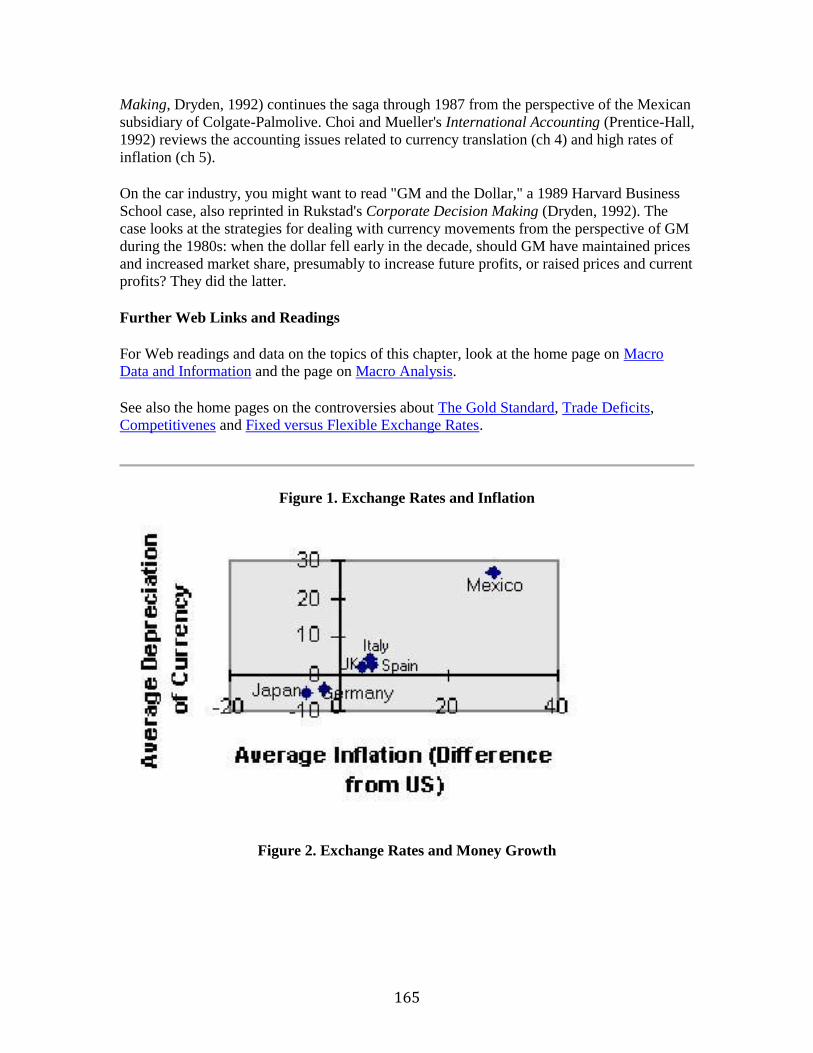
165

Making, Dryden, 1992) continues the saga through 1987 from the perspective of the Mexican

subsidiary of Colgate-Palmolive. Choi and Mueller's International Accounting (Prentice-Hall,

1992) reviews the accounting issues related to currency translation (ch 4) and high rates of

inflation (ch 5).

On the car industry, you might want to read "GM and the Dollar," a 1989 Harvard Business

School case, also reprinted in Rukstad's Corporate Decision Making (Dryden, 1992). The

case looks at the strategies for dealing with currency movements from the perspective of GM

during the 1980s: when the dollar fell early in the decade, should GM have maintained prices

and increased market share, presumably to increase future profits, or raised prices and current profits? They did the latter.

Further Web Links and Readings

For Web readings and data on the topics of this chapter, look at the home page on Macro Data and Information and the page on Macro Analysis.

See also the home pages on the controversies about The Gold Standard, Trade Deficits, Competitivenes and Fixed versus Flexible Exchange Rates.

Figure 1. Exchange Rates and Inflation

Figure 2. Exchange Rates and Money Growth

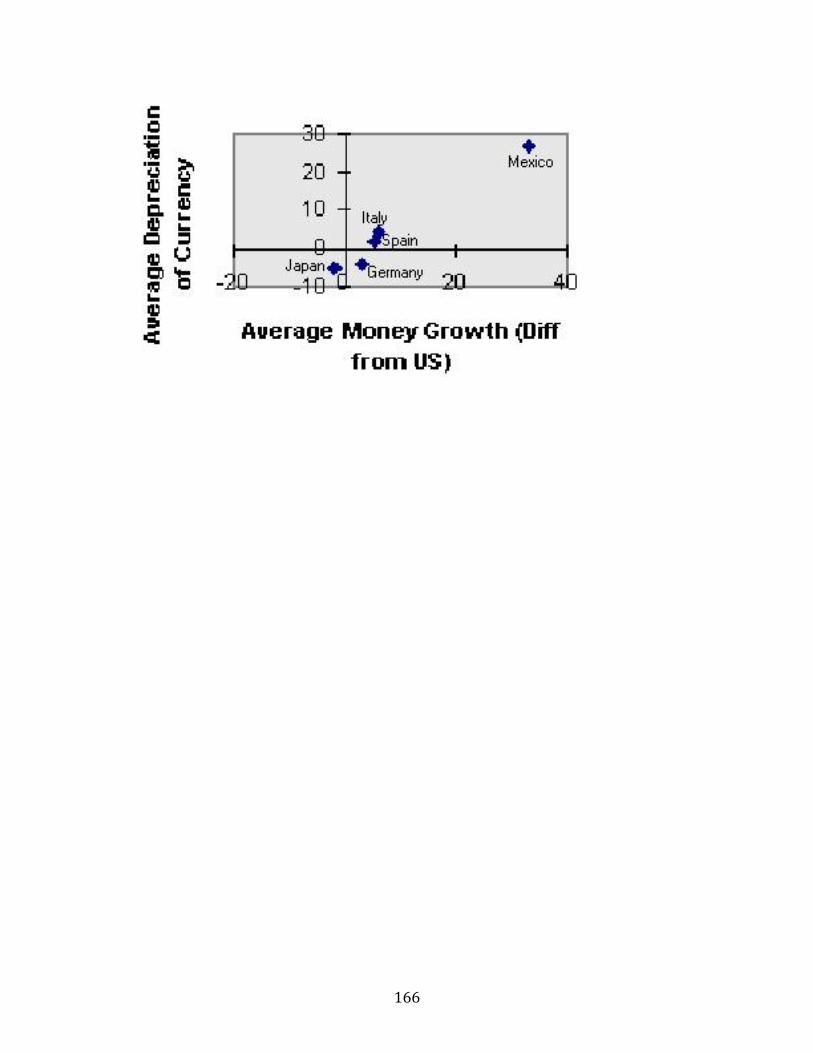
166

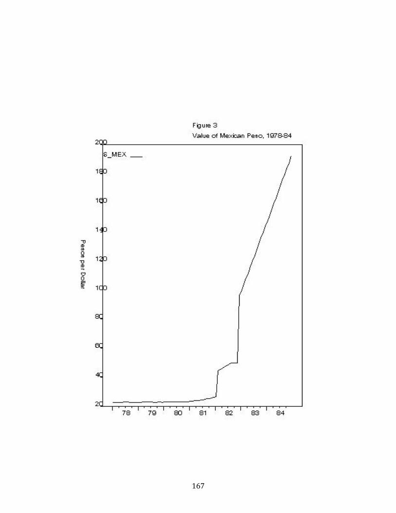
167

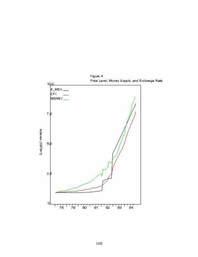
168

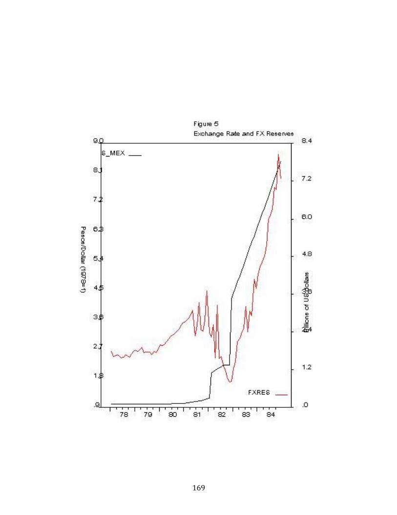
169

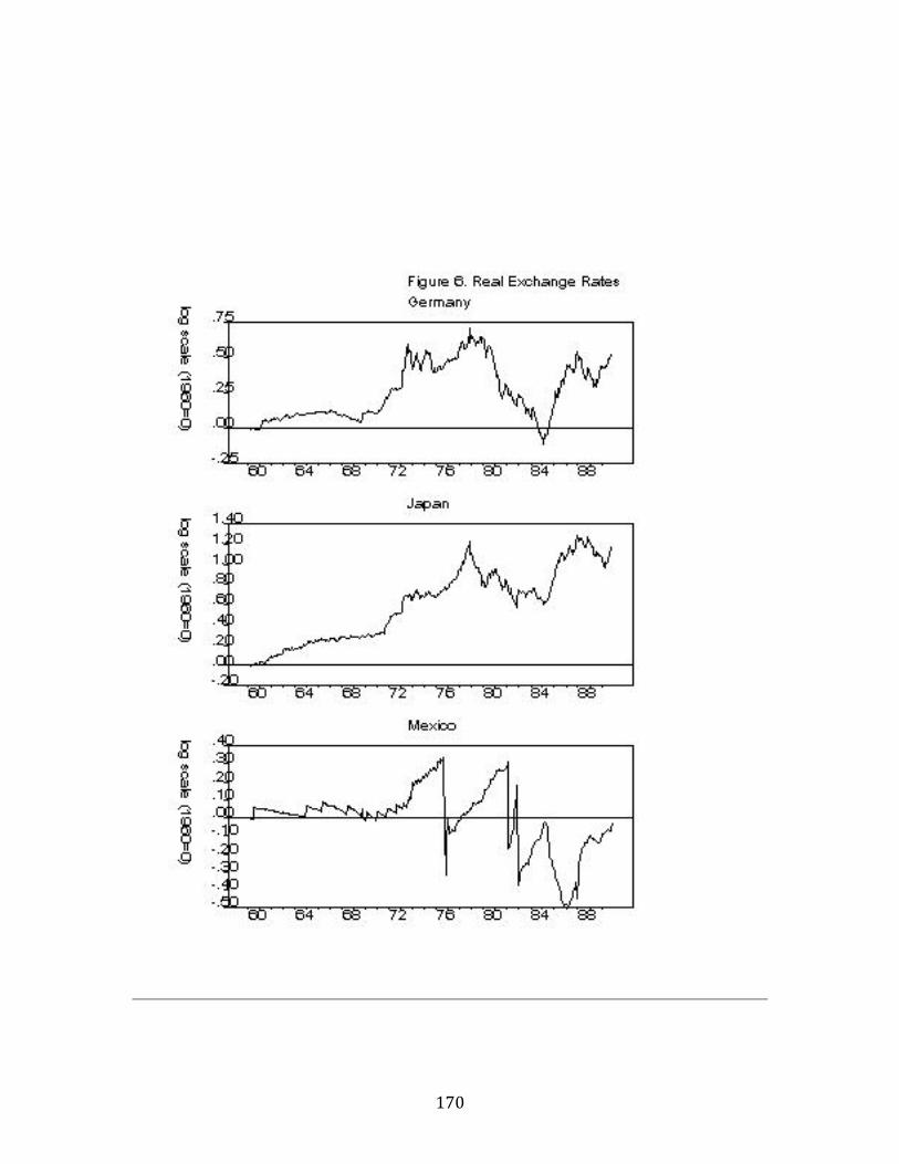
170

171

Copyright: Nouriel Roubini and David Backus, Stern School of Business, New York

University, 1997.

Chapter 8. Money, Interest Rates and Exchange Rates. The Collapse of Fixed Exchange

Rate Regimes. The Asian Currency Crisis of 1997.

Money Supply and the Determination of the Interest Rate

The Foreign Exchange Rate Market

The Effects of Open Market Operations Under Flexible and Fixed Exchange Rate

Regimes

The Joint Determination of the Interest Rate and Exchange Rate in the Money and

Exchange Rate Markets under Flexible Exchange Rates

Effect of Economic Shocks on the Exchange Rate Under Fixed Exchange Rate Regimes

Sterilized and Non-Sterilized Foreign Exchange Rate Intervention

Case Study of Fixed Exchange Rate Collapse: Mexico 1982

Why Countries Fix the Exchange Rate and Why Fixed Exchange Rates Collapse

The Asian Currency Crisis of 1997: An Empirical Analysis

Further Readings

In this chapter we will study a number of questions regarding the relation between monetary

policy, interest rates and exchange rates and how currency crises occur. How does monetary

policy affect interest rates? Why does a monetary expansion lead to lower interest rates?

What is the effect of monetary policy on exchange rates? Why do some countries try to fix

the level of their exchange rate while others let the value of their currency to be freely

determined in the foreign exchange market? How does monetary policy differ in a regime of

fixed and flexible exchange rates? After presenting the theory of currency crisis, we will analyze in detail the causes of the Asian currency crisis of 1997.

Money Supply and the Determination of the Interest Rate.

We consider first the equilibrium in the money market. The portfolio choice of individuals is

to decide how much to invest in various financial assets. Suppose, for simplicity, that an

investor has to decide how much to invest of her assets into money (cash balances that have a

zero interest rate return) and how much to invest into interest bearing assets (short term

Treasury bills).

Money (cash) balances have the disadvantage of not offering any nominal return (zero

interest rate); they have the advantage that you can use them to do transactions (buy/sell

goods). Short term bonds have the advantage that they earn interest; however, they have the

disadvantage that they cannot be used to make transactions (you need money to buy goods

and services). So, an investor will decide to allocate its portfolio between money and bonds considering the benefits and costs of both instruments.

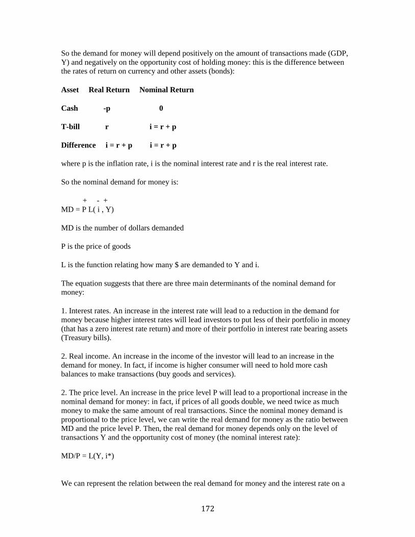
172

So the demand for money will depend positively on the amount of transactions made (GDP,

Y) and negatively on the opportunity cost of holding money: this is the difference between the rates of return on currency and other assets (bonds):

Asset Real Return Nominal Return

Cash -p 0

T-bill r i = r + p

Difference i = r + p i = r + p

where p is the inflation rate, i is the nominal interest rate and r is the real interest rate.

So the nominal demand for money is:

+ - +

MD = P L( i , Y)

MD is the number of dollars demanded

P is the price of goods

L is the function relating how many $ are demanded to Y and i.

The equation suggests that there are three main determinants of the nominal demand for money:

1. Interest rates. An increase in the interest rate will lead to a reduction in the demand for

money because higher interest rates will lead investors to put less of their portfolio in money

(that has a zero interest rate return) and more of their portfolio in interest rate bearing assets (Treasury bills).

2. Real income. An increase in the income of the investor will lead to an increase in the

demand for money. In fact, if income is higher consumer will need to hold more cash balances to make transactions (buy goods and services).

2. The price level. An increase in the price level P will lead to a proportional increase in the

nominal demand for money: in fact, if prices of all goods double, we need twice as much

money to make the same amount of real transactions. Since the nominal money demand is

proportional to the price level, we can write the real demand for money as the ratio between

MD and the price level P. Then, the real demand for money depends only on the level of transactions Y and the opportunity cost of money (the nominal interest rate):

MD/P = L(Y, i*)

We can represent the relation between the real demand for money and the interest rate on a

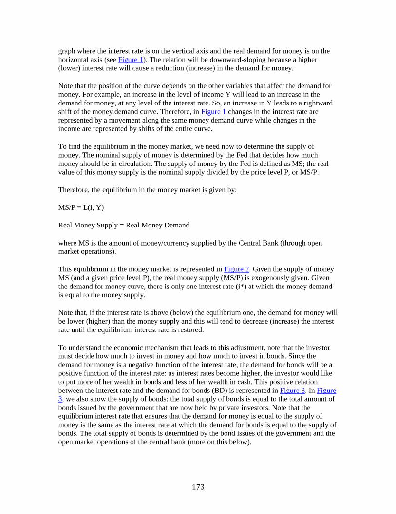
173

graph where the interest rate is on the vertical axis and the real demand for money is on the

horizontal axis (see Figure 1). The relation will be downward-sloping because a higher (lower) interest rate will cause a reduction (increase) in the demand for money.

Note that the position of the curve depends on the other variables that affect the demand for

money. For example, an increase in the level of income Y will lead to an increase in the

demand for money, at any level of the interest rate. So, an increase in Y leads to a rightward

shift of the money demand curve. Therefore, in Figure 1 changes in the interest rate are

represented by a movement along the same money demand curve while changes in the income are represented by shifts of the entire curve.

To find the equilibrium in the money market, we need now to determine the supply of

money. The nominal supply of money is determined by the Fed that decides how much

money should be in circulation. The supply of money by the Fed is defined as MS; the real value of this money supply is the nominal supply divided by the price level P, or MS/P.

Therefore, the equilibrium in the money market is given by:

MS/P = L(i, Y)

Real Money Supply = Real Money Demand

where MS is the amount of money/currency supplied by the Central Bank (through open market operations).

This equilibrium in the money market is represented in Figure 2. Given the supply of money

MS (and a given price level P), the real money supply (MS/P) is exogenously given. Given

the demand for money curve, there is only one interest rate (i*) at which the money demand is equal to the money supply.

Note that, if the interest rate is above (below) the equilibrium one, the demand for money will

be lower (higher) than the money supply and this will tend to decrease (increase) the interest rate until the equilibrium interest rate is restored.

To understand the economic mechanism that leads to this adjustment, note that the investor

must decide how much to invest in money and how much to invest in bonds. Since the

demand for money is a negative function of the interest rate, the demand for bonds will be a

positive function of the interest rate: as interest rates become higher, the investor would like

to put more of her wealth in bonds and less of her wealth in cash. This positive relation

between the interest rate and the demand for bonds (BD) is represented in Figure 3. In Figure

3, we also show the supply of bonds: the total supply of bonds is equal to the total amount of

bonds issued by the government that are now held by private investors. Note that the

equilibrium interest rate that ensures that the demand for money is equal to the supply of

money is the same as the interest rate at which the demand for bonds is equal to the supply of

bonds. The total supply of bonds is determined by the bond issues of the government and the open market operations of the central bank (more on this below).

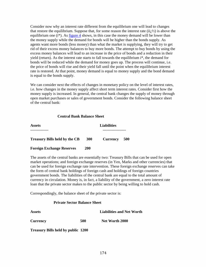
174

Consider now why an interest rate different from the equilibrium one will lead to changes

that restore the equilibrium. Suppose that, for some reason the interest rate (i�) is above the

equilibrium one (i*). As figure 4 shows, in this case the money demand will be lower than

the money supply while the demand for bonds will be higher than the bonds supply. As

agents want more bonds (less money) than what the market is supplying, they will try to get

rid of their excess money balances to buy more bonds. The attempt to buy bonds by using the

excess money balances will lead to an increase in the price of bonds and a reduction in their

yield (return). As the interest rate starts to fall towards the equilibrium i*, the demand for

bonds will be reduced while the demand for money goes up. The process will continue, i.e.

the price of bonds will rise and their yield fall until the point when the equilibrium interest

rate is restored. At that point, money demand is equal to money supply and the bond demand is equal to the bonds supply.

We can consider next the effects of changes in monetary policy on the level of interest rates,

i.e. how changes in the money supply affect short term interest rates. Consider first how the

money supply is increased. In general, the central bank changes the supply of money through

open market purchases or sales of government bonds. Consider the following balance sheet of the central bank:

Central Bank Balance Sheet

Assets Liabilities

-------------- ------------------

Treasury Bills held by the CB 300 Currency 500

Foreign Exchange Reserves 200

The assets of the central banks are essentially two: Treasury Bills that can be used for open

market operations; and foreign exchange reserves (in Yen, Marks and other currencies) that

can be used for foreign exchange rate intervention. These foreign exchange reserves can take

the form of central bank holdings of foreign cash and holdings of foreign countries

government bonds. The liabilities of the central bank are equal to the total amount of

currency in circulation. Money is, in fact, a liability of the government, a zero interest rate loan that the private sector makes to the public sector by being willing to hold cash.

Correspondingly, the balance sheet of the private sector is:

Private Sector Balance Sheet

Assets Liabilities and Net Worth

Currency 500 Net Worth 2000

Treasury Bills held by public 1200

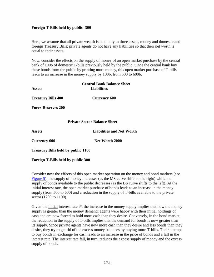
175

Foreign T-Bills held by public 300

Here, we assume that all private wealth is held only in three assets, money and domestic and

foreign Treasury Bills; private agents do not have any liabilities so that their net worth is equal to their assets.

Now, consider the effects on the supply of money of an open market purchase by the central

bank of 100b of domestic T-bills previously held by the public. Since the central bank buy

these bonds from the public by printing more money, this open market purchase of T-bills leads to an increase in the money supply by 100b, from 500 to 600b:

Central Bank Balance Sheet

Assets Liabilities

Treasury Bills 400 Currency 600

Forex Reserves 200

Private Sector Balance Sheet

Assets Liabilities and Net Worth

Currency 600 Net Worth 2000

Treasury Bills held by public 1100

Foreign T-Bills held by public 300

Consider now the effects of this open market operation on the money and bond markets (see

Figure 5): the supply of money increases (as the MS curve shifts to the right) while the

supply of bonds available to the public decreases (as the BS curve shifts to the left). At the

initial interest rate, the open market purchase of bonds leads to an increase in the money

supply (from 500 to 600) and a reduction in the supply of T-bills available to the private sector (1200 to 1100).

Given the initial interest rate i*, the increase in the money supply implies that now the money

supply is greater than the money demand: agents were happy with their initial holdings of

cash and are now forced to hold more cash than they desire. Conversely, in the bond market,

the reduction in the supply of T-bills implies that the demand for bonds is now greater than

its supply. Since private agents have now more cash than they desire and less bonds than they

desire, they try to get rid of the excess money balances by buying more T-bills. Their attempt

to buy bonds in exchange for cash leads to an increase in the price of bonds and a fall in the

interest rate. The interest rate fall, in turn, reduces the excess supply of money and the excess supply of bonds.

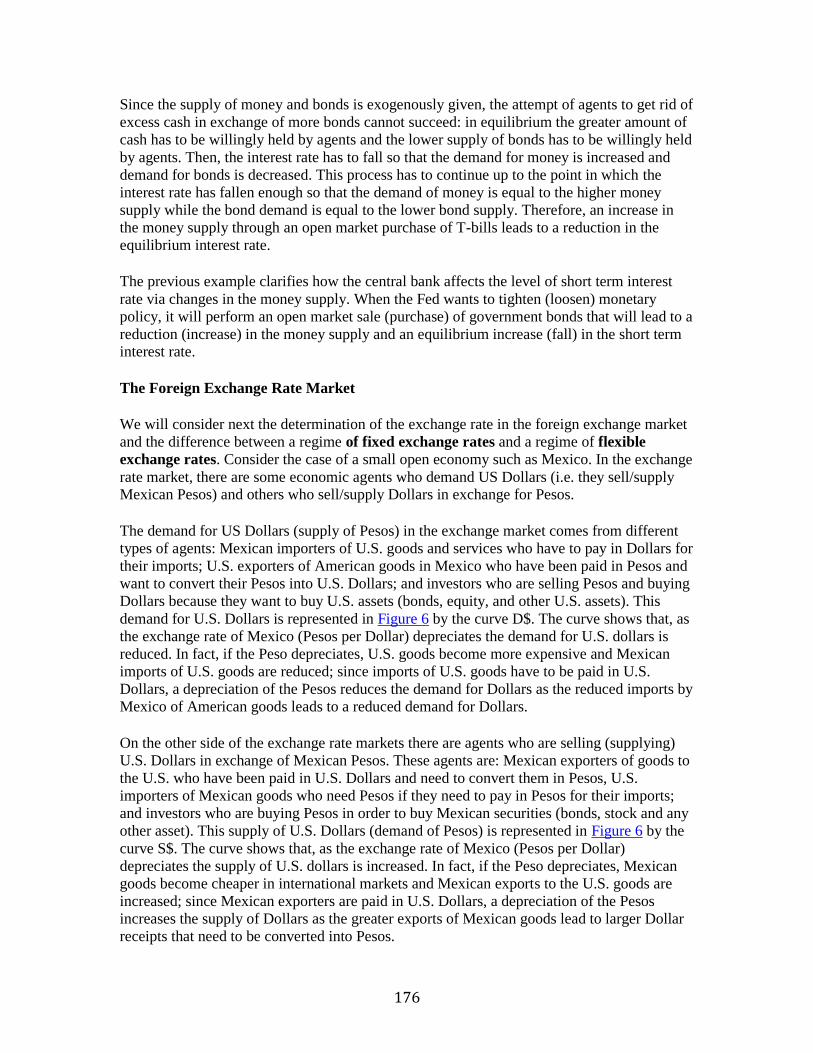
176

Since the supply of money and bonds is exogenously given, the attempt of agents to get rid of

excess cash in exchange of more bonds cannot succeed: in equilibrium the greater amount of

cash has to be willingly held by agents and the lower supply of bonds has to be willingly held

by agents. Then, the interest rate has to fall so that the demand for money is increased and

demand for bonds is decreased. This process has to continue up to the point in which the

interest rate has fallen enough so that the demand of money is equal to the higher money

supply while the bond demand is equal to the lower bond supply. Therefore, an increase in

the money supply through an open market purchase of T-bills leads to a reduction in the

equilibrium interest rate.

The previous example clarifies how the central bank affects the level of short term interest

rate via changes in the money supply. When the Fed wants to tighten (loosen) monetary

policy, it will perform an open market sale (purchase) of government bonds that will lead to a

reduction (increase) in the money supply and an equilibrium increase (fall) in the short term interest rate.

The Foreign Exchange Rate Market

We will consider next the determination of the exchange rate in the foreign exchange market

and the difference between a regime of fixed exchange rates and a regime of flexible

exchange rates. Consider the case of a small open economy such as Mexico. In the exchange

rate market, there are some economic agents who demand US Dollars (i.e. they sell/supply Mexican Pesos) and others who sell/supply Dollars in exchange for Pesos.

The demand for US Dollars (supply of Pesos) in the exchange market comes from different

types of agents: Mexican importers of U.S. goods and services who have to pay in Dollars for

their imports; U.S. exporters of American goods in Mexico who have been paid in Pesos and

want to convert their Pesos into U.S. Dollars; and investors who are selling Pesos and buying

Dollars because they want to buy U.S. assets (bonds, equity, and other U.S. assets). This

demand for U.S. Dollars is represented in Figure 6 by the curve D$. The curve shows that, as

the exchange rate of Mexico (Pesos per Dollar) depreciates the demand for U.S. dollars is

reduced. In fact, if the Peso depreciates, U.S. goods become more expensive and Mexican

imports of U.S. goods are reduced; since imports of U.S. goods have to be paid in U.S.

Dollars, a depreciation of the Pesos reduces the demand for Dollars as the reduced imports by

Mexico of American goods leads to a reduced demand for Dollars.

On the other side of the exchange rate markets there are agents who are selling (supplying)

U.S. Dollars in exchange of Mexican Pesos. These agents are: Mexican exporters of goods to

the U.S. who have been paid in U.S. Dollars and need to convert them in Pesos, U.S.

importers of Mexican goods who need Pesos if they need to pay in Pesos for their imports;

and investors who are buying Pesos in order to buy Mexican securities (bonds, stock and any

other asset). This supply of U.S. Dollars (demand of Pesos) is represented in Figure 6 by the

curve S$. The curve shows that, as the exchange rate of Mexico (Pesos per Dollar)

depreciates the supply of U.S. dollars is increased. In fact, if the Peso depreciates, Mexican

goods become cheaper in international markets and Mexican exports to the U.S. goods are

increased; since Mexican exporters are paid in U.S. Dollars, a depreciation of the Pesos

increases the supply of Dollars as the greater exports of Mexican goods lead to larger Dollar

receipts that need to be converted into Pesos.

177

Consider now the equilibrium in the exchange rate market: there is going to be an exchange

rate S (Pesos per Dollar) at which the demand for Dollars (supply of Pesos) is equal to the

supply of Dollars (demand for Pesos): this equilibrium exchange rate is S* in Figure 6.

Figure 7 shows that, if the initial Peso/Dollar exchange rate is depreciated relative to its

equilibrium value (i.e. S' > S*), the supply of Dollars will be greater than the demand for

Dollars (as Mexican exports are higher and their imports lower) and this will tend to

appreciate the Peso relative to the $. In the figure S will fall, meaning that the Peso will

appreciate until the equilibrium exchange rate S* is restored. The reverse will happen if the

initial S is below (appreciated relative to) the equilibrium one.

When a country has a regime of "flexible exchange rates", it will allow the demand and

supply of foreign currency in the exchange rate market to determine the equilibrium value of

the exchange rate. So the exchange rate is market determined and its value changes at every

moment in time depending on the demand and supply of currency in the market.

Some countries, instead, do not allow the market to determine the value of their currency.

Instead they "peg" the value of the foreign exchange rate to a fixed parity, a certain amount

of Pesos per Dollar. In this case, we say that a country has a regime of "fixed exchange

rates". In order to maintain a fixed exchange rate, a country cannot just announce a fixed

parity: it must also commit to defend that parity by being willing to buy (sell) foreign

reserves whenever the market demand for foreign currency is greater (smaller) than the supply of foreign currency.

To understand how fixed and flexible exchange rate regimes work suppose that, initially, the

exchange rate is equal to a value S* such that the demand and supply of foreign currency are

equal (see Figure 8). But, then, some shock occurs that leads to an increase in the demand for

foreign currency: for example, a boom in income in the domestic economy leads to an increase in imports that have to be paid in foreign currency.

Such a shock is represented in Figure 8 by a rightward shift in the demand for foreign

currency. If a country has a regime of flexible exchange rates, it will allow the increase in the

demand of foreign currency to cause a depreciation of the domestic currency: the equilibrium

exchange rate depreciates from S* to the new equilibrium value S'. Conversely, suppose that

the country has a regime of fixed exchange rates: in this case the country is committed to

defend the parity S*: it will not allow the currency to depreciate to S'.

How can a country avoid such a depreciation of its currency? Note that at the initial fixed

exchange rate S*, after the shock has occurred the market demand for foreign exchange is

greater than the market supply (D$' >S$). Therefore, in order to prevent a depreciation of the

domestic currency, the central bank of the country has to provide to the market an amount of

foreign exchange reserves equal to the difference between the market demand and the market

supply of Dollars. In other terms, the central bank has to sell foreign exchange reserves that it

was holding among its assets in order to prevent the currency depreciation.

In technical terms, the central bank intervenes in the foreign exchange rate market by selling

foreign currency. Therefore, a country can defend a fixed exchange rate parity that differs

from the equilibrium exchange rate (that would hold under flexible rates) only as long as it

has a sufficient amount of foreign exchange reserves to satisfy the market excess demand for

178

the foreign currency. If the country runs out of foreign exchange reserves, the fixed parity

becomes unsustainable and the central bank will be forced to give up the defense of the currency: the exchange rate will depreciate to its flexible rate value S'.

Note also that foreign exchange rate intervention affects the money supply of the country

under consideration. In fact, when the central bank intervenes to defend its parity, it is selling

foreign exchange currency to investors in the market; in exchange of its sale of foreign

currency the central bank receives domestic currency that is therefore taken out of

circulation: investors pay with domestic currency their purchase of foreign currency from the

central bank. In this sense, foreign exchange intervention taking the form of a sale of foreign

reserves has an effect on the money supply that is identical to an open market sale of

government securities; in both cases, the money supply is reduced. To see the effects of

foreign exchange intervention on the money supply, consider the following example.

Suppose the central bank intervenes in the foreign exchange rate market by selling 50b worth

of foreign reserves. Before, the intervention, the balance sheet of the private sector and central bank were:

Private Sector Balance Sheet

Assets Liabilities and Net Worth

Currency 600 Net Worth 2000

Treasury Bills held by public 1100

Foreign assets held by public 300

Central Bank Balance Sheet

Assets Liabilities

Treasury Bills 400 Currency 600

Forex Reserves 200

After the 50b sale of foreign exchange represented by the forex intervention:

Private Sector Balance Sheet

Assets Liabilities and Net Worth

Currency 550 Net Worth 2000

Treasury Bills held by public 1100

Foreign assets held by public 350

179

Central Bank Balance Sheet

Assets Liabilities

Treasury Bills 400 Currency 550

Forex Reserves 150

Therefore, foreign exchange rate intervention taking the form of a sale of foreign reserves

leads to a reduction in the money supply. Conversely, foreign exchange rate intervention

taking the form of a purchase of foreign reserves leads to an increase in the money supply.

The Effects of Open Market Operations Under Flexible and Fixed Exchange Rate

Regimes

We discussed above in the section on the money market equilibrium how open market

purchases and sales of domestic government bonds affect the money supply and the interest

rate of an economy. Open market operations are the standard way in which a central bank

controls the money supply and interest rates. We should consider now the effects of such

open market operations when the economy is open. We will show that open market operations have very different effects under flexible and fixed exchange rate regimes.

Consider first the effect of an open market purchase of government bonds under flexible

exchange rates. Under flexible rates, the central bank does not intervene to defend its

currency when market pressures lead to its weakening. Therefore, an open market purchase

of domestic bonds will lead to an increase of the money supply. In turn, this increase in the

money supply will cause a reduction of the domestic interest rate (see Figure 5 above). What

will be the effect of this monetary expansion on the exchange rate? The exchange rate will

depreciate: in fact, as interest rate at home are now lower than before, investors will want to

reduce their holding of domestic bonds and increase their holding of foreign bonds that are

now relatively more attractive in terms of their return. Therefore, domestic investors will try

to sell domestic bonds, buy foreign currency and buy foreign bonds. The attempt to sell

domestic currency in order to buy foreign bonds will, in turn, cause a depreciation of the domestic currency.

The effects of the open market purchase of bonds (say 50b) on the money supply under

flexible exchange rate will be identical to the one obtained in a closed economy: the money

supply will increase and interest rates will fall. As an example, before the open market purchase, the central bank balance sheet was:

Central Bank Balance Sheet

Assets Liabilities

Treasury Bills held by the CB 300 Currency 500

180

Foreign Exchange Reserves 200

After the open market operation:

Central Bank Balance Sheet

Assets Liabilities

Treasury Bills held by the CB 350 Currency 550

Foreign Exchange Reserves 200

The increase in the money supply and reduction in the interest rate will lead to a depreciation

of the domestic currency but since the central bank does not defend the current parity under

flexible exchange rates, no foreign reserve intervention will occur and foreign reserves will remain the same as before: then, the exchange rate will depreciate.

Consider next the effects of the same open market purchase of domestic bonds under fixed

exchange rates. We will show that, under a regime of fixed exchange rates, any attempt by

the central bank to increase the money supply via an open market operation is not going to be

successful: the central bank is not going to be able to change the money supply. The reason is

that, if the exchange rate is fixed, the equilibrium level of the money supply is determined

endogenously and cannot be affected by exogenous central bank open market operations. Let

us see why. We know from Chapter 3 that, under conditions of perfect capital mobility, the

uncovered interest rate parity condition holds, i.e. the domestic interest rate is equal to the foreign interest rate plus the expected depreciation of the domestic currency or:

i= i* + dS/S

Now, under fixed exchange rate, the exchange is not allowed to change: therefore the

expected depreciation of the domestic currency (dS/S) must be, by definition, equal to zero.

This also means that, under fixed exchange rate, the nominal interest rate of a small open

economy must always be equal to the world interest rate (i=i*): if it was lower, no one would

hold domestic bonds. Now consider how this equality of domestic and world interest rates

affects the equilibrium in the domestic money market. Assume that, in the short-run

framework here considered, the domestic output (Y) is constant and the domestic price level

(P) is constant. The equilibrium in the money market implies that real money demand must

be equal to real money supply:

M/P = L (Y, i) = L(Y, i*)

or:

M = P L(Y, i*)

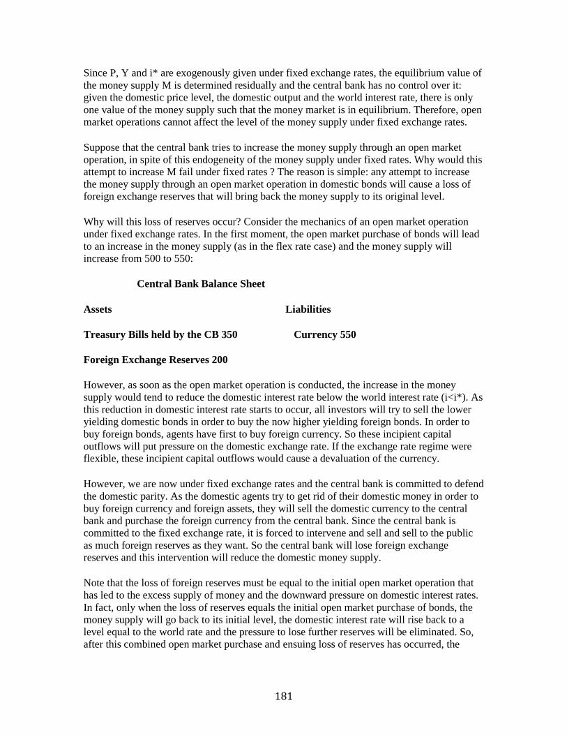
181

Since P, Y and i* are exogenously given under fixed exchange rates, the equilibrium value of

the money supply M is determined residually and the central bank has no control over it:

given the domestic price level, the domestic output and the world interest rate, there is only

one value of the money supply such that the money market is in equilibrium. Therefore, open market operations cannot affect the level of the money supply under fixed exchange rates.

Suppose that the central bank tries to increase the money supply through an open market

operation, in spite of this endogeneity of the money supply under fixed rates. Why would this

attempt to increase M fail under fixed rates ? The reason is simple: any attempt to increase

the money supply through an open market operation in domestic bonds will cause a loss of foreign exchange reserves that will bring back the money supply to its original level.

Why will this loss of reserves occur? Consider the mechanics of an open market operation

under fixed exchange rates. In the first moment, the open market purchase of bonds will lead

to an increase in the money supply (as in the flex rate case) and the money supply will increase from 500 to 550:

Central Bank Balance Sheet

Assets Liabilities

Treasury Bills held by the CB 350 Currency 550

Foreign Exchange Reserves 200

However, as soon as the open market operation is conducted, the increase in the money

supply would tend to reduce the domestic interest rate below the world interest rate (i<i*). As

this reduction in domestic interest rate starts to occur, all investors will try to sell the lower

yielding domestic bonds in order to buy the now higher yielding foreign bonds. In order to

buy foreign bonds, agents have first to buy foreign currency. So these incipient capital

outflows will put pressure on the domestic exchange rate. If the exchange rate regime were flexible, these incipient capital outflows would cause a devaluation of the currency.

However, we are now under fixed exchange rates and the central bank is committed to defend

the domestic parity. As the domestic agents try to get rid of their domestic money in order to

buy foreign currency and foreign assets, they will sell the domestic currency to the central

bank and purchase the foreign currency from the central bank. Since the central bank is

committed to the fixed exchange rate, it is forced to intervene and sell and sell to the public

as much foreign reserves as they want. So the central bank will lose foreign exchange

reserves and this intervention will reduce the domestic money supply.

Note that the loss of foreign reserves must be equal to the initial open market operation that

has led to the excess supply of money and the downward pressure on domestic interest rates.

In fact, only when the loss of reserves equals the initial open market purchase of bonds, the

money supply will go back to its initial level, the domestic interest rate will rise back to a

level equal to the world rate and the pressure to lose further reserves will be eliminated. So,

after this combined open market purchase and ensuing loss of reserves has occurred, the

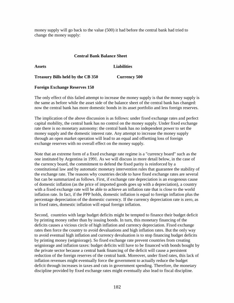
182

money supply will go back to the value (500) it had before the central bank had tried to

change the money supply:

Central Bank Balance Sheet

Assets Liabilities

Treasury Bills held by the CB 350 Currency 500

Foreign Exchange Reserves 150

The only effect of this failed attempt to increase the money supply is that the money supply is

the same as before while the asset side of the balance sheet of the central bank has changed: now the central bank has more domestic bonds in its asset portfolio and less foreign reserves.

The implication of the above discussion is as follows: under fixed exchange rates and perfect

capital mobility, the central bank has no control on the money supply. Under fixed exchange

rate there is no monetary autonomy: the central bank has no independent power to set the

money supply and the domestic interest rate. Any attempt to increase the money supply

through an open market operation will lead to an equal and offsetting loss of foreign

exchange reserves with no overall effect on the money supply.

Note that an extreme form of a fixed exchange rate regime is a "currency board" such as the

one instituted by Argentina in 1991. As we will discuss in more detail below, in the case of

the currency board, the commitment to defend the fixed parity is reinforced by a

constitutional law and by automatic monetary intervention rules that guarantee the stability of

the exchange rate. The reasons why countries decide to have fixed exchange rates are several

but can be summarized as follows. First, if exchange rate depreciation is an exogenous cause

of domestic inflation (as the price of imported goods goes up with a depreciation), a country

with a fixed exchange rate will be able to achieve an inflation rate that is close to the world

inflation rate. In fact, if the PPP holds, domestic inflation is equal to foreign inflation plus the

percentage depreciation of the domestic currency. If the currency depreciation rate is zero, as

in fixed rates, domestic inflation will equal foreign inflation.

Second, countries with large budget deficits might be tempted to finance their budget deficit

by printing money rather than by issuing bonds. In turn, this monetary financing of the

deficits causes a vicious circle of high inflation and currency depreciation. Fixed exchange

rates then force the country to avoid devaluations and high inflation rates. But the only way

to avoid eventual high inflation and currency devaluation is to stop financing budget deficits

by printing money (seigniorage). So fixed exchange rate prevent countries from creating

seigniorage and inflation taxes: budget deficits will have to be financed with bonds bought by

the private sector because a central bank financing of the deficit will cause a persistent

reduction of the foreign reserves of the central bank. Moreover, under fixed rates, this lack of

inflation revenues might eventually force the government to actually reduce the budget

deficit through increases in taxes and cuts in government spending. Therefore, the monetary

discipline provided by fixed exchange rates might eventually also lead to fiscal discipline.

183

The Joint Determination of the Interest Rate and Exchange Rate in the Money and

Exchange Rate Markets under Flexible Exchange Rates.

Let us consider now in more detail the equilibrium in the money market and in the foreign

exchange market under flexible exchange rates. In the money market, the equilibrium condition is the equality between real money supply and real money demand:

MS/P = L(Y, i) (1)

Equation (1) is represented graphically in Figure 2.

The equilibrium in the exchange rate market is given by the uncovered interest rate parity condition discussed in Chapter 3:

i = i* + {[Et(St+1)/ St]-1} (2)

Equation (2) implies that the return on domestic bonds must be equal to the total return on

holding foreign bonds; in turn, the latter is the sum of the return on foreign bonds plus the

expected percentage rate of depreciation (appreciation) of the domestic currency. For

example, if the foreign interest rate is 5% and investors expect a 2% depreciation of the

domestic currency, the total return to holding foreign bonds will be 7%, equal to the sum of

5% plus the 2% exchange rate capital gain deriving from holding a more appreciated

currency. We can represent the right hand side of equation (2) in Figure 9 where the

horizontal axis is the overall return on foreign assets and the vertical axis is current level of

the exchange rate (St). The curve is downward sloping for the following reason. Take today's

expectation of tomorrow's exchange rate Et(St+1) as given, say equal to 1. Then, if today�s

exchange rate is also equal to 1, the total return on the foreign asset is equal to i*, say 5%.

Suppose now that the expected future exchange rate remains equal to 1 while today's spot

exchange rate is now more appreciated than before, say equal to 0.95; then, the expected

depreciation of the domestic currency is equal to 5.2% ((1-0.95)/0.95) and the overall return

on the foreign asset is 10.2% (=5% + 5.2%). If the current spot exchange rate is 0.9 and the

expected future spot is still 1, the expected depreciation is equal to 11% ((1-0.9)/0.9) and the

overall return on the foreign assets is now equal to 16% (=5%+11%). In general the relation

between the overall return on the foreign asset and the current exchange rate is negative (as in

Figure 9) because, for a given expected future exchange rate, a more appreciated current spot

exchange rate (a smaller S) implies a larger expected depreciation and therefore a larger return on the foreign asset.

Equation (2) also tells us that if we know the value of the domestic and foreign interest rates

and the value of the expected future exchange rate, we can derive the equilibrium current

period spot exchange rate. To find this equilibrium exchange rate we have to put together

equation (1) (represented by Figure 2) that determines the domestic interest rate with

equation (2) that is presented in Figure 9. The combination of these two equilibria is

presented in Figure 10. The bottom part of Figure 10 presents the determination on the

nominal interest rate in the money market (this is Figure 2 rotated to the right in Figure 10):

given the exogenous real money supply, the real money demand curve determines the domestic interest rate at which money demand is equal to money supply.

184

Once we have found the equilibrium domestic interest rate, we can use equation (2)

represented in the top part of Figure 10 to find the equilibrium spot exchange rate. The

equilibrium spot rate S* is the value of today's exchange rate at which the return on domestic

assets is equal to the overall return on foreign assets. Given equation (2), once we know i, i*

and the expected future spot exchange rate (Et(St+1)), there is only one value of St such that

the return on domestic assets is equal to the return on foreign assets. For example, suppose

that, given the money supply and money demand, the equilibrium domestic interest rate is

10.2%. Then the value of St at which the return on domestic assets (10.2%) is equal to the

overall return on foreign assets is equal to 0.95. This equilibrium value of St is obtained by

finding the value of S at which the downward sloping curve i*+{[Et(St+1)/ St]-1} meets the vertical line representing the equilibrium domestic interest rate, as shown in Figure 10.

We can then discuss the effects on the exchange rate of a change in domestic monetary

policy. Suppose that, as shown in Figure 11, the domestic money supply is increased (via an

open market operation) form MS1 to MS2. Then, the equilibrium in the money market

requires a fall in the equilibrium domestic interest rate from the original i1 (=10.2%) to i2 (say

8.0% now). The Figure 11 shows that this monetary policy shock should cause a depreciation

of the domestic currency from the original S1 (the original 0.95) to S2 (in this case equal to

0.97). In fact, at the original (pre-shock) level of the exchange, the fall in the domestic

interest rate lead initially to a lower return on domestic asset relative to foreign assets. The

ensuing capital outflow causes the depreciation of the domestic currency. In summary, a

monetary expansion that leads to a reduction in domestic interest rates causes a depreciation of the domestic currency.

We can consider next the effects on the exchange rate of a number of other economic shocks.

Suppose that, for some reason, there is a shock that leads investors to expect that the

domestic exchange rate will depreciate in the future. To simplify things, assume that, before

this shock, agents were not expecting any depreciation of the exchange rate in the future, i.e.

Et(St+1)= St, and that both the actual and expected exchange rates were equal to 1. However,

after the shock occurs we have Et(St+1)=1.07>St=1 so that investors are now expecting a 7%

depreciation of the domestic currency. The effects of this change in expectations are

presented in Figure 12. The shock to expectations shifts to the right the curve representing the

overall return to foreign bonds: in fact, for any given current exchange rate, the change in

expectations increases the total return to foreign assets. Before the shock we had Et(St+1)= St;

therefore, the domestic interest rate was equal to the foreign interest rate (i=i*), say 5% as in

the Figure. The figure shows that the change in expectations about the future exchange rate

from 1 to 1.07 leads to an immediate depreciation of the current domestic exchange rate at

time t, from 1 to 1.07, i.e. the change in expectations leads to an immediate depreciation of

the domestic currency. The reason why a change in expectations about future exchange rates

leads to an immediate depreciation of the domestic currency is clear: when the change in

expectations occurs, given the initial exchange rate St still equal to 1, the expected return on

foreign assets goes up from 5% to 12% (=5% plus the expected depreciation of 7%). As

foreign assets are now expected to have a higher return than domestic assets (who are earning

only 5%), agents dump the domestic asset and currency in order to buy the higher yielding

foreign assets. This capital outflow leads to an instantaneous depreciation of the domestic

currency by 7%. Only when the current exchange rate falls from 1 to 1.07, the equilibrium in

the exchange rate market is restored. In fact, in the new equilibrium we have Et(St+1)= St= 1.07 and i=i*=5%.

185

The above example shows the importance of expectations for the determination of exchange

rates. Changes in expectations can have very rapid effect on the level of exchange rates.

Moreover, these changes in expectations may be the result not only of new information about

the fundamental future value of the domestic exchange rate. They can also be a result of pure

speculative factors: a change in the market mood or investors' beliefs about the future value

of a currency that is not based on true fundamental variables (such as change in current and

future economic conditions and interest rates). Exchange rates can then move for pure

speculative reasons: as in the example above, if the market starts to expect a future

devaluation of the domestic currency for whatever reason (rational or not), such a change in expectations will lead immediately to a self-fulfilling depreciation of the domestic currency.

Changes in other variables can also affect the domestic exchange rate. For example, an

increase at time t in the foreign interest rate i* has an effect on the domestic exchange rate

that is identical to that of a change in expectations described above. Initially, the increase in

the foreign interest rate leads to an increase in the expected return on foreign assets above the

return on domestic assets (a shift to the right of the curve representing the expected return on

foreign assets). This, in turn leads domestic investors to dump domestic assets and currency;

this capital outflow causes an immediate depreciation of the domestic currency. In the new

equilibrium the domestic currency depreciates by a percentage amount equal to the increase

in the foreign interest rate, i.e. if the foreign exchange interest rate goes from 5% to 8%, the

domestic currency depreciates by 3%. This effect of a higher foreign interest rate is

represented graphically in Figure 13.

Effect of Economic Shocks on the Exchange Rate Under Fixed Exchange Rate Regimes

As discussed above, under a regime of flexible exchange rates economic shocks such as a

change in foreign interest rates or an exogenous change in expectations about future

exchange rates lead to a devaluation of the domestic currency. What will be the effect of such shocks in a regime of fixed exchange rates?

In the discussion above on fixed exchange rates we argued that, in a regime of fixed

exchange rates, the central bank has no autonomous power to arbitrarily change the level of

the money supply. That, however, does not mean that the domestic money supply is always

constant under fixed rates. In fact, shocks to the variables that determine the demand for

money (i.e. shocks to the domestic price level, the domestic output and the world interest

rate) will, in equilibrium, force a change in the level of the money supply. The equilibrium in

the money market under fixed rates is given by:

M = P L(Y, i*)

For example, suppose that starting from an initial equilibrium, the foreign interest rate goes

up. The domestic interest rate will also increase and this will lead to a reduction of money

demand. To restore the equilibrium the money supply must also fall. How will this reduction

of the money supply be achieved? When the foreign interest rate goes up, the domestic

interest rate is initially unchanged: so agents try to sell domestic bonds and buy foreign

currency in order to buy the higher yielding foreign bonds. In order to prevent the currency

186

depreciation that this capital outflow would cause under flex rates, the central bank

intervenes and sells foreign currency. In turn, this intervention reduces the money supply and

leads to an increase in the domestic interest rate up to the new higher world interest rate. At

that point, the loss of reserves stops, the money supply is lower than before (as the forex

intervention took domestic liquidity out of circulation) and the domestic interest rate has risen to the level of the world interest rates.

Alternatively, the central bank could achieve the same reduction in the equilibrium level of

the money supply necessary to restore the equilibrium in the money market via an open

market sale of domestic government bonds rather than the above sale of foreign reserves.

Both actions lead to the same required result: the money supply is reduced and the domestic

interest rate goes up to the level of the world rate. In this example, open market operations

are effective in changing the money supply but this does not mean that the monetary

authority had any autonomous power to change the money supply. Quite to the contrary, the

initial increase in the world interest rate forces the central bank to engineer an equilibrium

reduction in the domestic money supply: this reduction can be achieved either through a loss

of foreign reserves or alternatively, if the central bank wants to avoid the reserve loss,

through a required open market operation that takes liquidity out of the market and pushes

the domestic interest rate up to the new world interest rate level. In this example, open market

operations do affect the money supply under fixed rates but not because the central bank has

an autonomous power to change the money supply: the central bank has to passively

intervene to adjust the money supply to the level required by higher world interest rate.

The effects of the increase in the foreign interest rate under fixed rates are presented

graphically in Figure 14. Initially, the increase in the foreign interest rate (say from 5% to

8%) leads to an increase in the total expected return on foreign assets, a shift to the right of

the curve representing foreign returns. Under flexible exchange rates, this change would lead

to a 3% depreciation of the domestic currency from 1 to 1.03. Under fixed rates, this

depreciation has to be prevented and the only way to do that is to have an increase in the

domestic interest rate from 5% to 8% to match the higher world interest rate. This increase in

the domestic interest rate is obtained by an endogenous reduction in the domestic money

supply from MS1 to MS2. How will this contraction in the money supply occur? Either the

central bank intervenes to defend the currency when the foreign interest rate goes up and this

intervention leads to a fall in the money supply; or, equivalently, the central bank performs

an open market sale of government bonds that reduces the liquidity in the economy. Both

actions have the effect of reducing the domestic money supply and increase the domestic interest rate to the higher world interest rate.

Another shock that might occur in a regime of fixed exchange rates is a change in

expectations that leads to an expected future depreciation of a fixed exchange rate. How

should monetary authorities that are trying to defend a fixed parity react to a change in

investors' sentiments about the credibility of the country commitment to fixed exchange

rates? To understand this case, one must first note that, under fixed exchange rates, the

exchange rate parity is constant. So, in normal times when the commitment to a fixed parity

is credible the future exchange rate is expected to remain equal to the current fixed parity as agents believe that the parity will not be changed.

187

However, being in a regime of fixed exchange rates does not mean that the fixed parity will

never be changed. For example, if the central bank runs out of reserves to defend the

currency, a devaluation might occur at some point. This means that a fixed parity may not be

fully credible in the sense that there is a positive probability that the future exchange rate will

be different from the current one if a devaluation occurs. In other terms, in spite of the

current fixity of the exchange rate, changes in the expectations about the future value of the

exchange rate might occur even in a regime of fixed exchange rates (that is not fully

credible). Such changes in expectations may be due to good reasons such as changes in

fundamental variables (high domestic inflation, large budget deficits, political risks and so

on) or might, at times, also be caused by "irrational" changes in the investors' sentiments.

Self-fulfilling changes in expectations may lead investors to believe that a fixed parity will

collapse and this will lead them to a speculative attack on a currency that has a fixed parity,

even if there has been no change in the underlying fundamental determinants of exchange

rates.

Then, the question to be addressed is the following: suppose that market investors start to

believe that a future devaluation of the fixed parity might occur, i.e. their expectation

becomes that the future exchange rate will be above the current fixed parity. Given this

change in expectations, what can a central bank do to prevent the devaluation of the exchange

rate from occurring? The answer to this question is simple: the central bank has to allow the

domestic interest rate to rise above the world interest rate to make sure that the capital

outflows induced by the expected depreciation of the domestic currency fail to materialize.

To see how an expected depreciation of the domestic currency must lead to higher interest rates in a regime of fixed rate consider Figure 15.

Suppose that, for whatever reason, there is a shock that leads investors to expect that the

domestic exchange rate will depreciate in the future. Assume that, before this shock, the fixed

rate regime was fully credible and agents were not expecting any depreciation of the

exchange rate in the future, i.e. Et(St+1)= St. For example, assume that both actual and

expected exchange rates were equal to 1. Since Et(St+1)= St, the domestic interest rate is

initially equal to the foreign interest rate (i=i*), say 5%. Now suppose that after the shock

occurs, market investors start to believe that a 7% future devaluation of the domestic

currency might occur; now we have Et(St+1)=1.07>St=1 as the fixed exchange rate parity is

not fully credible. The effect of this change in expectations is presented in Figure 15. The

shock to expectations shifts to the right the curve representing the overall return on foreign

bonds: for any given current exchange rate, the change in expectations increases the expected

return on foreign assets from 5 to 12% (5% plus the 7% expected devaluation). As discussed

in a previous section, if the economy was in a regime of flexible exchange rates, the change

in expectations about the future exchange rate from 1 to 1.07 would lead to an immediate

depreciation of the current domestic exchange rate at time t, from 1 to 1.07. In a regime of

fixed exchange rates, instead, such a devaluation of the currency must be prevented. As

Figure 15 shows, the only way to maintain the original exchange rate parity of 1 is to have an

increase in the domestic interest rate from 5% to 12%. In fact, given the shock to

expectations, domestic residents will not try to dump the domestic assets and currency in

favor of the foreign assets only as long as the domestic assets provide a return equal to the

expected return on foreign assets. Since the expected devaluation has increased the expected

return on foreign assets from 5% to 12% the domestic interest rate has to go up from 5% to 12%.

188

As the figure shows, the increase in the domestic interest rate is achieved through an

endogenous reduction in the domestic money supply from MS1 to MS2. As in the case

discussed before of an increase in the foreign interest rate, the reduction in the domestic

money supply can be achieved in two equivalent ways. Either the central bank intervenes to

defend the currency at the time when the change in expectations occurs and this intervention

leads to a fall in the money supply; or, equivalently, the central bank performs an open

market sale of government bonds that reduces the liquidity in the economy. Both actions

have the effect of reducing the domestic money supply and increase the domestic interest

rate. In the new equilibrium, the domestic interest rate has gone up from 5% to 12% while the

foreign interest rate i* is still equal to 5%. However, since investors expect a 7% depreciation

of the domestic currency, the expected total return to foreign assets is 12% and this is the

reason why the domestic interest rate must be now equal to 12% to make sure that a devaluation does not occur.

Sterilized and Non-Sterilized Foreign Exchange Rate Intervention

Suppose now that the defense of the domestic currency occurs, as it is usually the case,

through foreign exchange intervention: the central bank sells foreign reserves to the public

and this leads to a reduction in the money supply and an increase in domestic interest rates. Before the intervention the central bank balance sheet was:

Central Bank Balance Sheet

Assets Liabilities

Treasury Bills held by the CB 300 Currency 500

Foreign Exchange Reserves 200

After the open market operation the money supply falls from 500 to 450: Central Bank Balance Sheet

Assets Liabilities

Treasury Bills held by the CB 300 Currency 450

Foreign Exchange Reserves 150

This example of foreign exchange intervention is formally called "non-sterilized

intervention" since the central bank allows the intervention to affect the equilibrium level of the money supply in the domestic economy.

There is however another type of forex intervention that takes the name of "sterilized

intervention". To understand this type of intervention, suppose that you intervene in the

foreign exchange market; such intervention, if it is not sterilized, would lead to a reduction in

the money supply and an increase in domestic interest rates (as in Figures 14 and 15). Now

suppose that, after you intervene, you want to sterilize, i.e. you want to eliminate the effects

of your intervention on your money supply and interest rates. You might want to do that for a

189

number of reasons: for example high interest rate might lead the economy into a recession.

Then, how do you sterilize your intervention? The answer is that, after you intervene in the

forex market, you bring back the money supply to its previous level via an open market

purchase of domestic bonds. If you do that the central bank balance sheet becomes:

Central Bank Balance Sheet

Assets Liabilities

Treasury Bills held by the CB 350 Currency 500

Foreign Exchange Reserves 150

so that the money supply goes back to the level it had before the original forex intervention.

Central banks often attempt to sterilize the effects of their intervention in the forex market to

prevent changes in the domestic money supply and interest rates coming from such forex

interventions. However, such sterilization policies have the negative consequences: in fact, in

times when the domestic currency is subject to devaluation pressures, sterilized interventions

do not allow the intervention to increase the domestic interest rate. Therefore, sterilized

interventions do not eliminate the original cause for a pressure on the exchange rate. When

your currency is subject to devaluation pressures and you are trying to maintain fixed

exchange rates, the only way to defend the currency is to perform non-sterilized

interventions that reduce the money supply and increase interest rates so that the incentive to

dump domestic assets is eliminated. If your interventions are sterilized, you do not allow the

intervention to affect your money supply and interest rates. Therefore, such sterilized

interventions lead to further losses of foreign reserves as the original cause of the initial

pressure on the exchange rate (higher expected returns on foreign assets relative to domestic

assets) is not eliminated through higher domestic interest rates. So, if the market is telling

you that your money supply should be equal to 450 and your interest rates equal to 12%, your

attempt to keep the money supply at 500 will lead to further losses of forex reserves. In fact,

after the sterilized intervention described above, the foreign exchange rate reserves will further fall from 150 to 100 to push down the money supply to its equilibrium value of 450:

Central Bank Balance Sheet

Assets Liabilities

Treasury Bills held by the CB 350 Currency 450

Foreign Exchange Reserves 100

This means that the only way to avoid persistent and continuous losses of foreign reserves is

to allow the forex interventions to affect the money supply and interest rates, i.e. you should

perform non-sterilized interventions. This also means that, if sterilized interventions continue

(in spite of exogenous pressures on your exchange rates), these policies will lead to a

continuous fall of forex reserves and the eventual loss of all of them. However, when that

occurs, you do not have any more reserves to defend your currency and the fixed exchange

rate collapses. In other terms, a speculative attack on your currency leads to a loss of forex

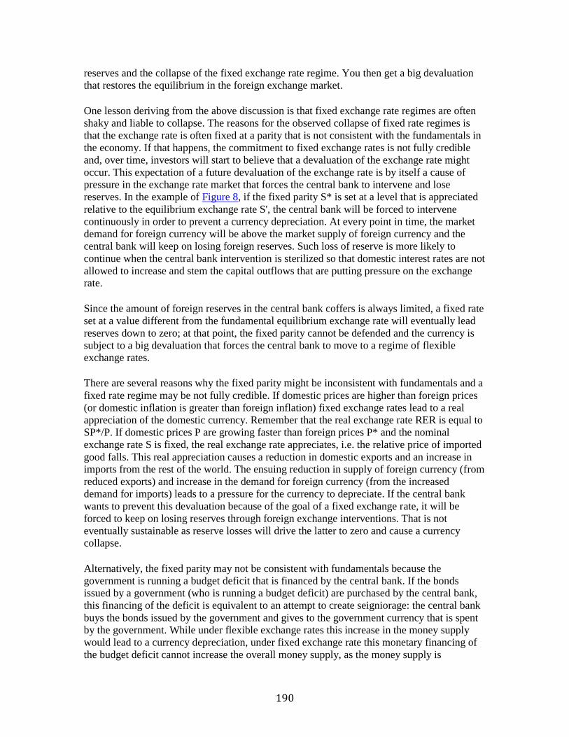
190

reserves and the collapse of the fixed exchange rate regime. You then get a big devaluation

that restores the equilibrium in the foreign exchange market.

One lesson deriving from the above discussion is that fixed exchange rate regimes are often

shaky and liable to collapse. The reasons for the observed collapse of fixed rate regimes is

that the exchange rate is often fixed at a parity that is not consistent with the fundamentals in

the economy. If that happens, the commitment to fixed exchange rates is not fully credible

and, over time, investors will start to believe that a devaluation of the exchange rate might

occur. This expectation of a future devaluation of the exchange rate is by itself a cause of

pressure in the exchange rate market that forces the central bank to intervene and lose

reserves. In the example of Figure 8, if the fixed parity S* is set at a level that is appreciated

relative to the equilibrium exchange rate S', the central bank will be forced to intervene

continuously in order to prevent a currency depreciation. At every point in time, the market

demand for foreign currency will be above the market supply of foreign currency and the

central bank will keep on losing foreign reserves. Such loss of reserve is more likely to

continue when the central bank intervention is sterilized so that domestic interest rates are not

allowed to increase and stem the capital outflows that are putting pressure on the exchange rate.

Since the amount of foreign reserves in the central bank coffers is always limited, a fixed rate

set at a value different from the fundamental equilibrium exchange rate will eventually lead

reserves down to zero; at that point, the fixed parity cannot be defended and the currency is

subject to a big devaluation that forces the central bank to move to a regime of flexible

exchange rates.

There are several reasons why the fixed parity might be inconsistent with fundamentals and a

fixed rate regime may be not fully credible. If domestic prices are higher than foreign prices

(or domestic inflation is greater than foreign inflation) fixed exchange rates lead to a real

appreciation of the domestic currency. Remember that the real exchange rate RER is equal to

SP*/P. If domestic prices P are growing faster than foreign prices P* and the nominal

exchange rate S is fixed, the real exchange rate appreciates, i.e. the relative price of imported

good falls. This real appreciation causes a reduction in domestic exports and an increase in

imports from the rest of the world. The ensuing reduction in supply of foreign currency (from

reduced exports) and increase in the demand for foreign currency (from the increased

demand for imports) leads to a pressure for the currency to depreciate. If the central bank

wants to prevent this devaluation because of the goal of a fixed exchange rate, it will be

forced to keep on losing reserves through foreign exchange interventions. That is not

eventually sustainable as reserve losses will drive the latter to zero and cause a currency collapse.

Alternatively, the fixed parity may not be consistent with fundamentals because the

government is running a budget deficit that is financed by the central bank. If the bonds

issued by a government (who is running a budget deficit) are purchased by the central bank,

this financing of the deficit is equivalent to an attempt to create seigniorage: the central bank

buys the bonds issued by the government and gives to the government currency that is spent

by the government. While under flexible exchange rates this increase in the money supply

would lead to a currency depreciation, under fixed exchange rate this monetary financing of

the budget deficit cannot increase the overall money supply, as the money supply is

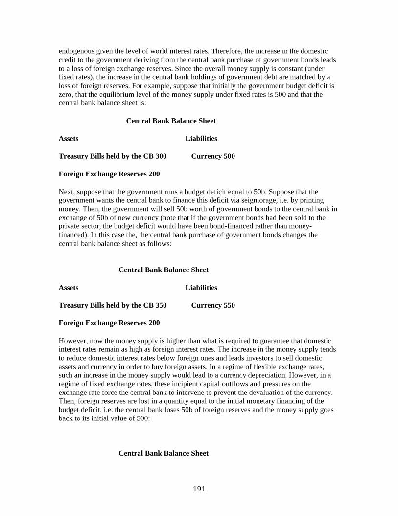
191

endogenous given the level of world interest rates. Therefore, the increase in the domestic

credit to the government deriving from the central bank purchase of government bonds leads

to a loss of foreign exchange reserves. Since the overall money supply is constant (under

fixed rates), the increase in the central bank holdings of government debt are matched by a

loss of foreign reserves. For example, suppose that initially the government budget deficit is

zero, that the equilibrium level of the money supply under fixed rates is 500 and that the central bank balance sheet is:

Central Bank Balance Sheet

Assets Liabilities

Treasury Bills held by the CB 300 Currency 500

Foreign Exchange Reserves 200

Next, suppose that the government runs a budget deficit equal to 50b. Suppose that the

government wants the central bank to finance this deficit via seigniorage, i.e. by printing

money. Then, the government will sell 50b worth of government bonds to the central bank in

exchange of 50b of new currency (note that if the government bonds had been sold to the

private sector, the budget deficit would have been bond-financed rather than money-

financed). In this case the, the central bank purchase of government bonds changes the

central bank balance sheet as follows:

Central Bank Balance Sheet

Assets Liabilities

Treasury Bills held by the CB 350 Currency 550

Foreign Exchange Reserves 200

However, now the money supply is higher than what is required to guarantee that domestic

interest rates remain as high as foreign interest rates. The increase in the money supply tends

to reduce domestic interest rates below foreign ones and leads investors to sell domestic

assets and currency in order to buy foreign assets. In a regime of flexible exchange rates,

such an increase in the money supply would lead to a currency depreciation. However, in a

regime of fixed exchange rates, these incipient capital outflows and pressures on the

exchange rate force the central bank to intervene to prevent the devaluation of the currency.

Then, foreign reserves are lost in a quantity equal to the initial monetary financing of the

budget deficit, i.e. the central bank loses 50b of foreign reserves and the money supply goes

back to its initial value of 500:

Central Bank Balance Sheet

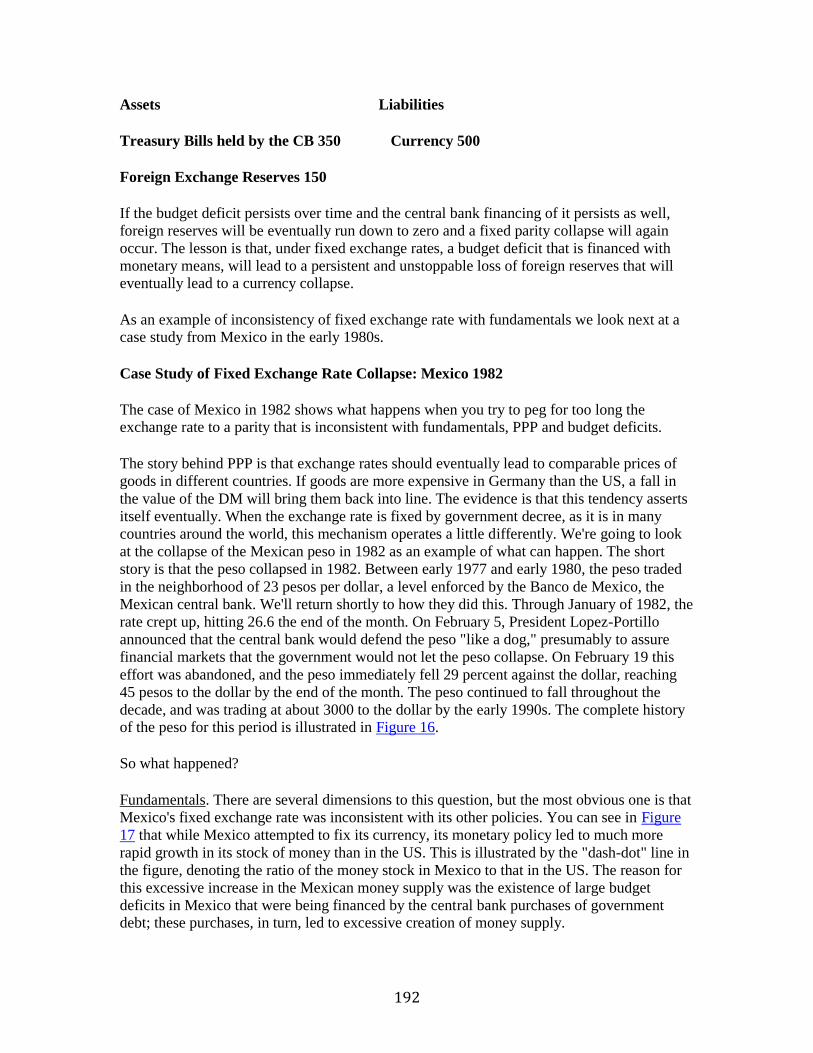
192

Assets Liabilities

Treasury Bills held by the CB 350 Currency 500

Foreign Exchange Reserves 150

If the budget deficit persists over time and the central bank financing of it persists as well,

foreign reserves will be eventually run down to zero and a fixed parity collapse will again

occur. The lesson is that, under fixed exchange rates, a budget deficit that is financed with

monetary means, will lead to a persistent and unstoppable loss of foreign reserves that will eventually lead to a currency collapse.

As an example of inconsistency of fixed exchange rate with fundamentals we look next at a

case study from Mexico in the early 1980s.

Case Study of Fixed Exchange Rate Collapse: Mexico 1982

The case of Mexico in 1982 shows what happens when you try to peg for too long the exchange rate to a parity that is inconsistent with fundamentals, PPP and budget deficits.

The story behind PPP is that exchange rates should eventually lead to comparable prices of

goods in different countries. If goods are more expensive in Germany than the US, a fall in

the value of the DM will bring them back into line. The evidence is that this tendency asserts

itself eventually. When the exchange rate is fixed by government decree, as it is in many

countries around the world, this mechanism operates a little differently. We're going to look

at the collapse of the Mexican peso in 1982 as an example of what can happen. The short

story is that the peso collapsed in 1982. Between early 1977 and early 1980, the peso traded

in the neighborhood of 23 pesos per dollar, a level enforced by the Banco de Mexico, the

Mexican central bank. We'll return shortly to how they did this. Through January of 1982, the

rate crept up, hitting 26.6 the end of the month. On February 5, President Lopez-Portillo

announced that the central bank would defend the peso "like a dog," presumably to assure

financial markets that the government would not let the peso collapse. On February 19 this

effort was abandoned, and the peso immediately fell 29 percent against the dollar, reaching

45 pesos to the dollar by the end of the month. The peso continued to fall throughout the

decade, and was trading at about 3000 to the dollar by the early 1990s. The complete history of the peso for this period is illustrated in Figure 16.

So what happened?

Fundamentals. There are several dimensions to this question, but the most obvious one is that

Mexico's fixed exchange rate was inconsistent with its other policies. You can see in Figure

17 that while Mexico attempted to fix its currency, its monetary policy led to much more

rapid growth in its stock of money than in the US. This is illustrated by the "dash-dot" line in

the figure, denoting the ratio of the money stock in Mexico to that in the US. The reason for

this excessive increase in the Mexican money supply was the existence of large budget

deficits in Mexico that were being financed by the central bank purchases of government debt; these purchases, in turn, led to excessive creation of money supply.

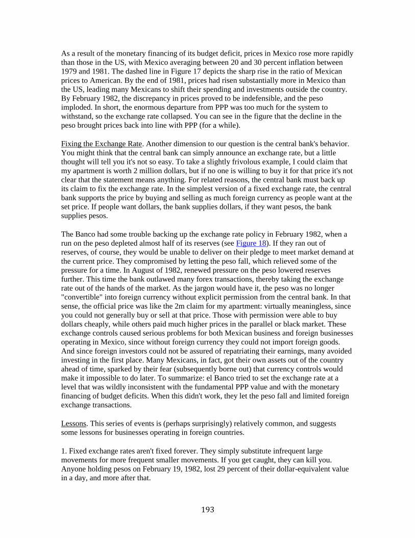
193

As a result of the monetary financing of its budget deficit, prices in Mexico rose more rapidly

than those in the US, with Mexico averaging between 20 and 30 percent inflation between

1979 and 1981. The dashed line in Figure 17 depicts the sharp rise in the ratio of Mexican

prices to American. By the end of 1981, prices had risen substantially more in Mexico than

the US, leading many Mexicans to shift their spending and investments outside the country.

By February 1982, the discrepancy in prices proved to be indefensible, and the peso

imploded. In short, the enormous departure from PPP was too much for the system to

withstand, so the exchange rate collapsed. You can see in the figure that the decline in the

peso brought prices back into line with PPP (for a while).

Fixing the Exchange Rate. Another dimension to our question is the central bank's behavior.

You might think that the central bank can simply announce an exchange rate, but a little

thought will tell you it's not so easy. To take a slightly frivolous example, I could claim that

my apartment is worth 2 million dollars, but if no one is willing to buy it for that price it's not

clear that the statement means anything. For related reasons, the central bank must back up

its claim to fix the exchange rate. In the simplest version of a fixed exchange rate, the central

bank supports the price by buying and selling as much foreign currency as people want at the

set price. If people want dollars, the bank supplies dollars, if they want pesos, the bank supplies pesos.

The Banco had some trouble backing up the exchange rate policy in February 1982, when a

run on the peso depleted almost half of its reserves (see Figure 18). If they ran out of

reserves, of course, they would be unable to deliver on their pledge to meet market demand at

the current price. They compromised by letting the peso fall, which relieved some of the

pressure for a time. In August of 1982, renewed pressure on the peso lowered reserves

further. This time the bank outlawed many forex transactions, thereby taking the exchange

rate out of the hands of the market. As the jargon would have it, the peso was no longer

"convertible" into foreign currency without explicit permission from the central bank. In that

sense, the official price was like the 2m claim for my apartment: virtually meaningless, since

you could not generally buy or sell at that price. Those with permission were able to buy

dollars cheaply, while others paid much higher prices in the parallel or black market. These

exchange controls caused serious problems for both Mexican business and foreign businesses

operating in Mexico, since without foreign currency they could not import foreign goods.

And since foreign investors could not be assured of repatriating their earnings, many avoided

investing in the first place. Many Mexicans, in fact, got their own assets out of the country

ahead of time, sparked by their fear (subsequently borne out) that currency controls would

make it impossible to do later. To summarize: el Banco tried to set the exchange rate at a

level that was wildly inconsistent with the fundamental PPP value and with the monetary

financing of budget deficits. When this didn't work, they let the peso fall and limited foreign

exchange transactions.

Lessons. This series of events is (perhaps surprisingly) relatively common, and suggests some lessons for businesses operating in foreign countries.

1. Fixed exchange rates aren't fixed forever. They simply substitute infrequent large

movements for more frequent smaller movements. If you get caught, they can kill you.

Anyone holding pesos on February 19, 1982, lost 29 percent of their dollar-equivalent value in a day, and more after that.

194

2. Operate in hard currencies when you can. One strategy for dealing with such risk is to do

business in dollars, or some other hard currency. US banks, for example, denominated their

loans in dollars, so the collapse in the peso did not hurt them on its own. But the collapse of

the economy that went with the fall in the peso did hurt them, with the result that most loans

were repaid only in part. Mexicans, too, tried to switch to dollars, but government restrictions made this difficult to do on a large scale.

3. Enter after the fall. A colleague of George Soros's said once that the best opportunities

come when situations change from "disaster" to "bad". Anyone entering the Mexican market in late 1982 or 1983 had, at least, the advantage of buying low.

Why Countries Fix the Exchange Rate and Why Fixed Exchange Rates Collapse

We observed before that it is often quite hard to permanently fix exchange rates and that

fixed exchange rate regime often collapse with a big devaluation. So why do countries like to fix their exchange rates? There are many reasons:

1. Under flexible exchange rates, the exchange rate might be affected by speculative factors

that have little to do with fundamentals. These speculative factors might lead to excessive

exchange rate volatility, misalignments of the nominal and real exchange rate from their

equilibrium level and negative effects of production, trade and investment. High exchange

rate volatility might increase the risk of assets and investment in a country and also reduce real trade in goods.

2. Flexible exchange rate leads to "beggar thy neighbour" policies where countries try to gain

competitive advantage for their exports through policies of devaluation of the domestic

currency. This is a source of conflict among countries since devaluation exchange rate policies may be a substitute for protectionist trade policies.

3. Flexible exchange rates may be a cause of high inflation (p) and fixed exchange rates

allow a country to converge very fast to low levels of international inflation. This is very important. Suppose that the PPP holds either in the short-run or the long-run. Then:

P = S Pf

In growth rates, the domestic inflation rate (p) is equal to the foreign inflation rate (pf)plus the rate of exchange rate depreciation (dS/S)

p = dS/S +pf 100% = 97% + 3%

Suppose that world inflation is low (3%) while our small open economy is stuck in a high

inflation equilibrium where inflation is 100%, and therefore the rate of depreciation is 97%

per year (100% - 3%). In this small economy all prices, wages and nominal variables are

growing at 100% per year, nominal interest rates are high (say 105 = 100% inflation plus 5%

real rate) and the economy is stuck in this high inflation bad equilibrium. In this economy,

wages are effectively indexed to inflation (either formally or informally) and all costs/price are growing at a nominal 100% rate.

195

Suppose that now we decide to fix the exchange rate to its current level. Then,

instantaneously, the rate of currency depreciation goes to zero. In a true PPP world the inflation goes instantaneously down to the world level:

P = S Pf

p = dS/S +pf 3% = 0%+ 3% = 3%

Since, with a fixed exchange rate S the price of imported good is now growing only at 3%

per year, the cost of imported good and inputs in production also falls to 3% right away. With

imported goods prices growing at 3% domestic firms cannot afford any more to increase

prices at 100% per year since no one would buy the domestic goods and everyone would

switch to the cheaper foreign goods. As prices of goods start to grow at 3% only, nominal

wage growth will also fall right away to 3% since workers have now no reason to ask for a

100% increase in their nominal wages: a 3% increase will maintain their real wage constant

over time. So in this ideal world, fixing the exchange rate is a miraculous and instantaneous

cure for inflation. This cure occurs at zero cost since nothing should happen on the real side

of the economy when the exchange rate is pegged. In particular, the real exchange rate is not

affected since in the old equilibrium the 97% depreciation was necessary to cover the 97%

inflation differential while now the inflation differential is zero so that no devaluation is needed to maintain a competitive nominal and real exchange rate:

RER = S Pf / P

Rate of % change or RER = dS/S +pf -p = 0 = 97 + 3 - 100

= 0 = 0 + 3 - 3

So, the big advantage of fixed exchange rates is that is a quick way to gain credibility in your

attempt to reduce inflation from very high levels to very low levels in a country that is otherwise stuck historically in a bad high inflation equilibrium.

So, what is the problem with the above strategy of using the exchange rate as a nominal

anchor for inflation expectations ?

While fixing the exchange rate is a fast way to disinflate an economy starting with high

inflation, pegging the exchange rate will not reduce the inflation rate instantaneously to the

world level. Inflation will fall a lot and very fast but maybe not right away to the 3% world

level. Suppose inflation falls from 100% to 8% in a very short period of time but then

remains at the 8% for a while. The reason why inflation will not fall all the way to 3% are many:

1. PPP does not hold exactly in the short run since domestic and foreign goods are not

perfectly substitutable. So domestic firms will reduce their price inflation down from 100%

to a much lower level but may not push it down to the world level. So some inflation above 3% will remain on domestic goods.

196

2. Since many wages are set in multi-year contract that are renewed only over time, the wage

inflation might not fall right away to 3%. Many wage contracts were based on the old

expected inflation (100%) and the adjustment of wages will occur slowly. Also, in countries

where there is formal indexation of nominal wages, wage inflation is based on past (higher)

inflation rather than current (lower) inflation; so this inertia in the wage setting in the

economy means that wage inflation will remain above 3% for a while and therefore costs of production (and prices) will increase more than 3% for a while.

So, assume that inflation falls from 100% down to 8% when you fix your exchange rate.

Then, the differential between domestic and foreign inflation is 5% (8% - 3%). Since now the

exchange rate is fixed, even a small differential of inflation rates implies that domestic prices

are growing faster than foreign imported good prices and therefore the real exchange rate is appreciating by 5% per year:

Rate of % change or RER = dS/S +pf - p = -5% = 0 + 3 - 8%

This appreciation of the real exchange rate implies a loss of competitiveness of the domestic

economy: domestic country exports become more expensive relative to imported goods; this

leads to a reduction in exports and an increase in imports that worsen the trade balance and the current account.

Now, while a 5% real appreciation seems pretty small, the point to notice is that is builds

over time. 5% real appreciation per year means that the real appreciation is going to be 10%

in 2 years, 15% in 3 years, 20% in 4 year and so on. So, an initial small real appreciation

becomes very large when the exchange rate is strictly fixed while the domestic inflation has

not converged to the world rate. Such a real appreciation will eventually cause very large

trade deficits. Example: Mexico had a quasi fixed exchange rate relative to the dollar

between 1990 and 1994. Since inflation in Mexico was about 5% above the US one, over

those five years this implied a real appreciation of the Mexican Peso of about 25% relative to

the parity of 1990. As a consequence, the current account that was close to balance in 1990 went to a 28 billion $ deficit by the end of 1994.

So, the problem of anti-inflation stabilization policies that use the fixed exchange rate as the

policy tool to fight inflation is that fixed rates lead to a real exchange rate appreciation and to a significant worsening of the current account.

One way to avoid the real appreciation of the currency in the transition to fix rates is to make

sure that once inflation is down to 8% and there is a 5% inflation differential, the central bank

allows the currency to depreciate at a 5% rate; i.e. instead of having strictly fixed rates, you

follow a policy of crawling peg where the rate of crawl (currency depreciation) per year is

limited to the remaining inflation differential (5%). Such a crawling peg exchange rate rule

prevents an inflation differential from causing a real appreciation that is bad for the trade balance.

Countries that do not like the idea of following a crawling peg and who stick instead to

tightly fixed rates argue that a crawling peg accommodates the inflation differential between

home and the world and does not allow a full convergence of domestic inflation to the world

level. So, it is argued that it is better to stick with completely fixed exchange rates to break as

197

fast as possible the back of inflation and push faster to the world level. The problem with

such a tough inflation and exchange rate policy is that, if there are in the economy structural

factors that lead to a persistent wage and price inertia, the inflation rate will not fully

converge to the world level and the lingering differential will cause a significant and progressively larger real appreciation and trade worsening.

So while a crawling peg prevents domestic inflation from fully converging to the world rate,

it also prevents the real exchange rate from appreciating. A variant of the crawling peg would

be to have a rate of crawl lower than the inflation differential (say 3% rather than the 5%

inflation differential): the advantage of variant is that since the rate of crawl does not fully

accommodate the inflation differential, domestic firms and workers will be pressed over time

to reduce their price and wage inflation; on the other side, a rate of crawl of 3% will lead to

some real appreciation and worsening of the trade balance but the real appreciation would not

be as large as in the case of a totally fixed nominal exchange rate. Mexico and many

European countries in the European Monetary System, however, kept their exchange rates tightly fixed and ended up with a huge real appreciation.

Now, if a fixed exchange rate leads over time to real appreciation and a worsening current

account deficit, the fixity of the exchange rate becomes less and less sustainable (and less and

less credible) over time. After a year of real appreciation, the current account deficit can be

easily financed through foreign borrowing (capital inflows). Such inflows are eagerly flowing

into the country in the early stages of the exchange rate stabilization since domestic rates are

higher than world ones and there is no risk of depreciation since s id fixed. So, you get

actually huge capital inflows that keep your currency strong. But over the years, as the real

appreciation becomes worse and the current account keeps on worsening you need more and

more foreign capital inflows to finance your current account deficit. In late stages of the

drama, investors start to realize that your fixed rate is not sustainable and start to believe that

a devaluation might occur. This expected depreciation leads to an increase in the expected

return on foreign assets and, for given domestic interest rates, leads to capital outflows. Then

the domestic foreign reserves of the central bank start to fall as it intervenes in the exchange

rate market to defend its currency from depreciating. If the foreign exchange intervention is

not sterilized, higher domestic interest rate are helpful to stabilize the exchange rate for a

while. If the FX intervention is sterilized , the pressure on the exchange rate remains and the

central bank keep on hemorrhaging its foreign reserves. As the doomsday approaches, the

expected depreciation becomes more likely and its probability of occurring higher. Then the

loss of reserves occurs at an even faster rate as capital outflows are occurring while the

current account is worse and worse. When you finally have lost most of your foreign

reserves, the exchange rate collapses and you move to flexible exchange rate. The speculative attack on your currency leads to a sharp and large devaluation of the exchange rate.

An example of the story just described is the case of the Mexican Peso in the 1990s that is

discussed in detail in the Mexican case study. The attempt to peg the parity of the Peso in the early 1990s eventually led to a dramatic collapse of the Mexican currency in December 1994.

The Asian Currency Crisis of 1997 (See the paper by Roubini, Corsetti and Pesenti on the Causes of the Asian Crisis for a more detailed analysis of the issues discussed in this section)

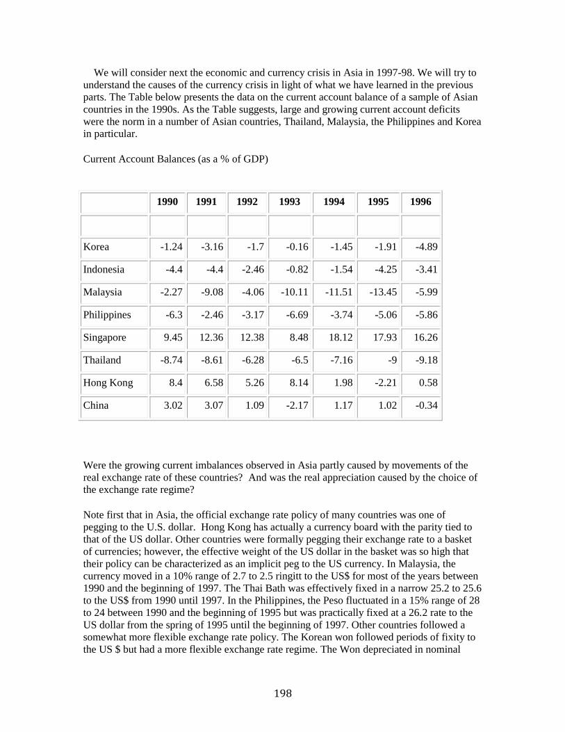
198

We will consider next the economic and currency crisis in Asia in 1997-98. We will try to

understand the causes of the currency crisis in light of what we have learned in the previous

parts. The Table below presents the data on the current account balance of a sample of Asian

countries in the 1990s. As the Table suggests, large and growing current account deficits

were the norm in a number of Asian countries, Thailand, Malaysia, the Philippines and Korea in particular.

Current Account Balances (as a % of GDP)

1990 1991 1992 1993 1994 1995 1996

Korea -1.24 -3.16 -1.7 -0.16 -1.45 -1.91 -4.89

Indonesia -4.4 -4.4 -2.46 -0.82 -1.54 -4.25 -3.41

Malaysia -2.27 -9.08 -4.06 -10.11 -11.51 -13.45 -5.99

Philippines -6.3 -2.46 -3.17 -6.69 -3.74 -5.06 -5.86

Singapore 9.45 12.36 12.38 8.48 18.12 17.93 16.26

Thailand -8.74 -8.61 -6.28 -6.5 -7.16 -9 -9.18

Hong Kong 8.4 6.58 5.26 8.14 1.98 -2.21 0.58

China 3.02 3.07 1.09 -2.17 1.17 1.02 -0.34

Were the growing current imbalances observed in Asia partly caused by movements of the

real exchange rate of these countries? And was the real appreciation caused by the choice of the exchange rate regime?

Note first that in Asia, the official exchange rate policy of many countries was one of

pegging to the U.S. dollar. Hong Kong has actually a currency board with the parity tied to

that of the US dollar. Other countries were formally pegging their exchange rate to a basket

of currencies; however, the effective weight of the US dollar in the basket was so high that

their policy can be characterized as an implicit peg to the US currency. In Malaysia, the

currency moved in a 10% range of 2.7 to 2.5 ringitt to the US$ for most of the years between

1990 and the beginning of 1997. The Thai Bath was effectively fixed in a narrow 25.2 to 25.6

to the US$ from 1990 until 1997. In the Philippines, the Peso fluctuated in a 15% range of 28

to 24 between 1990 and the beginning of 1995 but was practically fixed at a 26.2 rate to the

US dollar from the spring of 1995 until the beginning of 1997. Other countries followed a

somewhat more flexible exchange rate policy. The Korean won followed periods of fixity to

the US $ but had a more flexible exchange rate regime. The Won depreciated in nominal

199

terms from 1990 until the beginning of 1993 (from 700 to almost 800 won per dollar); next, it

traded in a very narrow range of 800 to 770 won/$ between the beginning of 1993 and the

middle of 1996. Then, it started to depreciate by about 10% reaching a rate of 884 at the end

of 1996. The Indonesian policy can be described as a policy of explicit real exchange rate

targeting with the nominal rate falling from 1900 rupieh to the US $ in 1990 to 2400 by the

beginning of 1997. Taiwan also followed a policy of real exchange rate targeting allowing its

currency to fall from a rate of 24 New Taiwan dollars per US$ in 1990 to a rate of 27.8 by the

end of 1996. In Singapore, the currency actually appreciated in nominal terms throughout the

1990s going from a rate of 1.7 in 1990 to a rate of 1.4 by the end of 1996. Finally, in China

where inflation was in the double digits in the early 1990s, the currency was allowed to

modestly depreciate between 1990 and 1993 but was drastically devalued by almost 50% in

1994; since then, the currency remained stable with a slight drift towards a nominal appreciation.

While such policy of pegging the exchange rate ensured in many Asian countries ensured the

stability of the nominal exchange rate relative to the US currency, it also had the consequence

that change in the nominal and real value of the dollar relative to the Japanese Yen and the

European currencies had the consequence of affecting the real exchange rate of the Asian

currencies pegged to the US dollar. Specifically, the dollar was on a downward nominal trend

relative to the yen and mark between 1991 and 1995 reaching a low of 80 yen per dollar in

the spring of 1995. During that period, the Asian currencies pegged to the U.S. experienced a

real depreciation of their currencies, as they were depreciating relative to the Japanese and

European currencies. However, after the spring of 1995, the dollar started to rapidly

appreciated relative to most world currencies (the yen/dollar rate went from 80 in the spring

to 1995 to over 125 in the summer of 1997, a 56% appreciation). As a consequence, the

Asian currencies that were tied in nominal terms to the dollar also experienced a very rapid

real appreciation.

Note also that a real exchange rate appreciation (from large capital inflows or any other

reason) may cause a loss of competitiveness and a structural worsening of the trade balance

which makes the current account deficit less sustainable. Thus, the current account deficit

may be less sustainable when accompanied by a real exchange rate appreciation that leads to

a misaligned currency value. In the case of Asia, the real appreciation might have been the

consequence of the choice of the exchange rate regime, essentially a fixed peg to the U.S.

dollar. The consequence of such a peg was that they led to large capital inflows attracted by

favorable interest rate differentials and the expectation of low exchange rate risk given the

policy of stable currency value. Such inflows prevented currency depreciations even if

domestic inflation was higher than world inflation and at times led to nominal currency

appreciation; this, in turn led to a real appreciation that was partly the cause of the large and

growing current account imbalances.

As discussed above, a real appreciation of the currency may occur when the exchange rate is

pegged and used as a nominal anchor for monetary policy (as it has been in most Asian

countries) if the initial domestic inflation rate is above the world one and it does not converge

rapidly to the world inflation rate. Therefore, the problem of anti-inflation stabilization

policies that use the fixed exchange rate as the policy tool to fight inflation is that fixed rates

lead to a real exchange rate appreciation and to a significant worsening of the current

account. While the Asian countries had not experienced the large inflation rates of some

200

Latin countries, their inflation rates were usually above those of the OECD group; therefore a

policy of pegged parities might have contributed to the real appreciation observed in the 1990s.

If we look at the data on the real exchange rate of the Asian countries, we see the following.

Taking 1990 as the base year, we observe that by the spring of 1997 the real exchange rate

had appreciated by 19% in Malaysia, 23% in the Philippines, 12% in Thailand, 8% in

Indonesia, 18% in Singapore, 30% in Hong Kong. In Korea, the currency had depreciated in

real terms by 14% while in Taiwan there was a 10% real depreciation. Find data on China

(real depreciation). This suggests that, with the exception of Korea, all the currencies that

crashed in 1997 had experienced a significant amount of real appreciation. Note also that in

several countries, a large part of the real appreciation occurred after 1995 in the period in which the dollar (to which these currencies were pegged) was becoming stronger.

It is important to note that the degree of real exchange rate appreciation seems to be

correlated with the choice of the exchange rate regime: countries with a more fixed exchange

rate regime experienced a much larger real appreciation. Conversely, countries such as

Korea, Taiwan and China that followed a more flexible exchange rate regime experience a

real depreciation. Note that Indonesia, that followed a regime closer to real exchange rate

targeting, the degree of real appreciation was smaller than that of countries such as Thailand,

Malaysia, Hong Kong and the Philippines that followed more closely regimes of fixed exchange rates.

The data also suggest that the degree of overvaluation was correlated with worsening of the

current account: countries with more overvalued currencies were generally experiencing a

larger worsening of the current account; while countries such as China and Taiwan that had

experienced a real depreciation had current account surpluses. The exception was Korea that

had large and increasing current account deficits while its currency had depreciated in real terms in the 1990s.

By early 1997, it was clear that several regional currencies were seriously overvalued and

that such overvaluation was a factor in the worsening of the current account of many

countries in the region. Real depreciations appeared to be necessary to adjust the current account position of the deficit countries.

It is important to not that in the 1990s there were several other factors that affected the

competitive positions of the Asian currencies. First of all, the 50% nominal of the Chinese

currency in 1994 led to a sharp real depreciation of the renminbi; the ensuing large and

growing trade surpluses of China led to a significant loss of competitiveness in the rest of

Asia. During the 1990s China, with wage level at a fraction of those in the rest of the region,

started to produce and compete in many manufacturing sectors that had been the source of

export growth for the East Asian countries. Second, after 1995 the rapid appreciation of the

dollar led to a significant real appreciation of the Asian currencies that were pegged to it.

Third, in 1995-96 there was a slump in the world demand for semi-conductors, one of

important export products in the region. This led to a significant reduction in export growth

by the region in 1996. Fourth, the continued economic weakness of Japan, that remained in a

state of economic stagnation throughout the 1990s dampened the demand for regional

exports, as over 30% of the Asian exports were going to the region.

201

Therefore, while the degree of real appreciation of the Asian currencies in the 1990s was not

as large as the one observed in previous episodes of currency collapse (such as Mexico in

1994), the combination of the factors discussed above made the competitive position of most

Asian countries quite fragile by the beginning of 1997.

In order to understand the currency crisis in 1997 and its spread from one country to the

other, it is important to note that the measures of the real exchange rate presented above do

not fully measure the competitiveness loss suffered by regional currencies whose currency

had not yet depreciated once some countries in the region had started to devalue. Take for

example the case of the Korean won. As many countries in the region compete in similar

products in world and regional markets (US, Europe and Japan), when the currencies of

Thailand, Malaysia, Indonesia and the Philippines started to depreciate over the summer

while the Korean won remained relatively stable until October, this implied a significant loss

of competitiveness for the Korean exporters. Specifically, if we take the end of 1996 as the

base period, by the end of September 1997, the Thai Baht had depreciated relative to the US$

by 42%, the Indonesian Rupiah by 37%, the Malaysian Ringitt by 26%, the Philippines Peso

by 28%. The Korean won, instead, by the end of September had depreciated only by 8%

(relative to December 1996). This implied that by the end of September, the won had

appreciated in nominal (and real) terms by 34%, 29%, 20% and 18%, relative to the

currencies of Thailand, Indonesia, the Philippines and Malaysia respectively. If we look at

the official figures for the real exchange rate of the won we do not observe the drastic loss of

competitiveness of the won between July and the end of September as such data are based on

aggregate trade-weighted (with 1990 base) data. While the official real exchange rate of the

won is stable over that period, Korea actually suffered a dramatic loss of competitiveness

during the summer months because the large devaluations of its regional trade competitors implied an effective real appreciation of the won and loss of competitive position

This effect of the depreciation of some regional currency on the "effective" real exchange

rate and competitiveness of the other countries in the regions is a crucial element to

understand why the currency contagion was importantly determined by fundamental factors.

As one after the other, the currencies of countries that were competing in the same world

market came under attack and started to depreciate, the equilibrium fundamental value of

other currencies that had not depreciated yet started to become lower and the pressure on

such currencies to depreciate to regain some of the competitiveness loss became even higher.

This game of competitive devaluations is the fundamental factor that explains why the currency contagion and the domino effects were driven by fundamental factors.

Throughout the crisis a number of factors exacerbated the fundamentals that were feeding the currency crisis.

First, the currency depreciation worsened the real burden of external debt faced by governments, financial institutions and firms that had heavily borrowed in foreign currency.

Second, the financial problems faced by firms and financial institutions were repeatedly

discovered to be far worse than originally announced generating significant uncertainty about

the depth and breadth of the financial problems faced by firms and banks; then, the currency

depreciation engineered by such uncertainty would ex-post worsen such financial conditions

and validate further weakenings of the currencies.

202

Third, the fundamental domino effect described above where the currency devaluation in one

country implied a worsening of the real appreciation of countries that had not depreciated yet

transmitted speculative pressures to one currency after the other: in July and August, the fall

of the baht spread to the ringitt, rupiah and the peso; by September, the contagion had spread

to Singapore and Taiwan. Once the later two currencies fell, the speculative pressure spread

within days to Hong Kong. By October, with six major currencies in the region having

devalued by an average 40%, the Korean won could not maintain a parity that was now out of

line with fundamentals. In turn, the sharp collapse of the won in November and December

led to a significant real appreciation in the other regional currencies that was not sustainable

given the shaky financial conditions of the countries; this is why such currencies continued to

fall in November and December on the heels of the won crisis with each depreciation round

feeding a spiral of the next series of depreciations. The persistent fall of the currencies of

Thailand, Indonesia and the Philippines even after large bail-out packages had been arranged

in the fall was certainly affected, among other factors, by the collapse of the won in November and December.

Fourth, significant political uncertainty led to serious policy uncertainty throughout the crisis.

The government weakness, cabinet reshufflings and eventual government collapse in

Thailand; the inflammatory statements by Malaysian PM against "rogue speculators"; the

elections in Indonesia, political tensions and continued bad news about the health of the

Indonesian president Suharto who has no apparent successor; the presidential elections and

contradictory policy signals sent by then candidate (and eventually President elect) Kim Dae

Jung; the threat of labor unrest in the region were all factors that added to the seriousness of the crisis.

Fifth, the economic problems of Japan, the leading regional economic exacerbated the crisis

in a number of ways: 1) In 1996 it appeared that an economic recovery was returning in

Japan after five years of zero growth but the increase in the consumption tax in April 1997

spinned Japan in another economic recession: second and third quarter economic activity

declined. 2) The economic weakness in Japan kept monetary policy loose, interest rate very

low and induced a continued depreciation of the yen relative to the US $ that exacerbated in

the first part of 1997 the real appreciation faced by the other regional currency; the crisis

finally exploded in the summer when the dollar was going through what seemed an

unstoppable rise and the yen continued its decline. 3) Japanese banks, already in a fragile

conditions after the burst of the 1980s asset bubble and weakened by a stagnant economy in

the 1990s had heavily lent to other Asian economies. Therefore, the currency shock in Asia,

the ensuing worsening of the financial conditions of Asian banks and firms and the ongoing

bankruptcy of an increasing number of them implied a worsening of the financial conditions

of Japanese banks and securities firm. Compared to the Mexican crisis of 1994-95 when the

US, the major regional economic power was in a strong cyclical upswing, the weakness of Japan in 1997 exacerbated poor economic fundamentals in the region.

Sixth, the first reaction of the monetary authorities to the speculative pressures on the

currencies was to try to avoid a monetary contraction and a significant increase in domestic

interest rates. When the first pressures started in the spring, the reaction in Thailand and other

countries was to perform sterilized interventions and, once such interventions turned out to be

ineffective given their sterilized nature, several countries introduced capital controls to

prevent capital outflows. The basic stance of monetary policy in the region remained quite

203

loose well into the crisis; it is only when the fall of the currencies accelerated in the fall that a

serious monetary tightening started to be implemented. For example, Malaysia waited until

early December when the ringitt had already fallen by over 40% to officially changed its

monetary stance and renounce its policy of low interest rates.

The reasons why governments delayed a monetary tightening and increase in interest rate that

could have slowed down capital outflow and the currency fall were several. First, an interest

rate increase would have led to a slowdown in economic activity that could turn recessionary.

Second, given the fragility of the banking system and of the corporate sector, a monetary

tightening would have led to a credit squeeze, corporate and banking bankruptcies and further

negative effects on the level of economic activity. On the other side, a relatively loose

monetary policy aimed at preventing further financial problems for firms and banks turned to

worsen things because it led to a continuous spiral of currency depreciation that dramatically

increased the real burden of the large foreign debt liabilities. At the end, when currencies

kept on falling, monetary authorities were forced to tighten monetary and credit conditions.

Paradoxically, such late tightening made things even worse because it came after the

depreciations had already sharply increased the real external liabilities of the borrowers and it

therefore led to a credit squeeze that increased the amount of non-performing loans,

exacerbated the financial problems of banks and firms and was a source of a sharp deflationary effect on the level of real economic activity.

In order to understand the magnitude an depth of the financial crisis in 1997, it is very

important to notice that the amounts of speculative capital inflows in Asia in the early 1990s

was much larger than the already large figures presented above about the size of the net

capital inflows. In fact, the estimates presented above of "other debt-creating net capital

inflows" (portfolio assets, bonds, equity and bank borrowings) give a misleading and

underestimated picture of the actual amount of speculative short-term capital inflows that

occurred in the 1990s. When one looks at the data, one observes that gross inflows of short-

term capital were significantly larger than the net inflows as there were large amounts of

gross short-term capital outflows as well. To give an example, consider Korea in 1996 that is

typical of the other countries' trends. In 1996, the current account deficit was $23b. As shown

in Chapter 3, net FDI inflows were negative to the tune of $2.1b. As foreign reserves

increased by 1.4b, net capital inflows were by definition equal to $24.4b. However, the gross

amount of capital inflows was much larger than $24.4b and actually equal to $41.3b; the difference between the two is the amount of gross financial capital outflows.

This is important because while, on a net basis, the increase in the external debt of the Asian

countries was equal to the current account deficit (minus the non-debt creating net FDI

inflows), the increase in the gross external liabilities of these countries was significantly

larger in the 1990s as large short-term capital inflows were also accompanied by very large

capital outflows. This increase in gross external liabilities became a serious issue in 1997

because, once the currency crisis started, large gross capital outflows exacerbated the crisis in two ways.

First, as the currencies were falling, non-residents were repatriating the capital inflows by

dumping domestic bonds, equities and other financial assets; on the other side, resident who

had accumulated large stocks of financial capital abroad via the large capital outflows of the

1990s were unwilling to repatriate such foreign currency outflows as their domestic

204

currencies were falling. Therefore, the degree of currency depreciation was magnified by the

existence of a previous large stock of non-resident owned gross domestic assets that had been accumulated over the decade via large gross capital inflows.

Second, a large fraction of the gross capital inflows and outflows were in the banking sector.

For example, in 1996 in Korea, of the $23.3b "other investment capital inflows", $12.3 went

to the banking sector while of the $11.8b "other investment capital outflows", $9.5b were

made by the banking system. This is consistent with the BIS data presented above that show

a much larger increase in liabilities towards BIS reporting banks (gross capital inflows) than

the increase in assets towards BIS reporting banks (gross capital outflows). This process of

large gross intermediation of capital inflows and outflows through the banking system

implied that the domestic Asian bank were increasing their foreign short-term liabilities

towards BIS banks much faster than their foreign assets. For example in Korea, at the end

1993 the liabilities of the domestic banks towards BIS banks were equal to $34.6b while their

foreign assets (towards BIS banks) were equal to 13.7b, for a net liability position of 20.8b.

But, between the end of 1993 and the second quarter of 1997, the gross liabilities went up to

$90.6b, a whopping increase of $56b in only three years and six months; the gross assets

went up to only to $33.5b, an increase of $19.8b. As a consequence, the net liability position

of the Korean banking system went from $20.8b at the end of 1993 to $57.0b by 1997:2, an

increase of $36.2b. Note that similarly large increases in gross external liabilities of the

banking and non-banking system are observed, controlling for country scale, in the other

countries in the region where a currency crisis occurred, especially Thailand, Malaysia, Philippines and Indonesia.

The increase in the gross liabilities of the banking system in the 1990s was an independent

cause of the worsening of the crisis and currency depreciation in 1997. For example, in

Korea, once the real burden of the heavy gross borrowing by banks and non-banks was

worsened by the depreciation of the currency and some financial institutions started to go

bankrupt, a financial panic ensued. Since it was not clear which banks were solvent and

which were not, foreign banks that had heavily lent to Korean banks started to refused to roll-

over the loans that would have been automatically renewed in normal times. The foreign

banks unwillingness to roll-over normal lines of credit in face of high risks of bankruptcy

made the prospect of loans default more likely and led to a situation of financial panic where

the currency collapsed in a week in December by over 40%; the currency collapse in turn

made the default more likely. The situation calmed down only around Christmas when, faced

with the prospect of a default induced by a self-fulfilling unwillingness to roll-over short-

term debts, the American, European and Japanese banks jointly agreed to negotiate an

orderly renewal of such short-term loans and the major creditor countries decided to anticipate a fraction of the bail-out package approved by the IMF in early December.

A similar cycle of currency crisis leading to a debt crisis was experienced by Indonesia: the

continuous depreciation of the domestic currency increased the real burden of the large gross

borrowing by banks and firms. As a consequence, financial panic emerged in Indonesia in early January 1998.

Summary of the Analysis

205

In summary, our analysis of the causes of the Asian crisis in suggests the following

conclusions.

First, several Asian currencies had appreciated in real terms in the 1990s and large and

growing current account imbalances had emerged in the countries that faced a speculative

attack in 1997. The overvaluation was due in part to the widespread choice of fixed exchange

rate regimes in the region and the related large capital inflows in the1990s. By early 1997, it

was clear that several regional currencies were seriously overvalued and that such

overvaluation was a factor in the worsening of the current account of many countries in the

region. Real depreciations appeared to be increasing needed to adjust the current account position of the deficit countries.

Second, the current account imbalances and related growth of foreign debt was also driven by

an investment boom (as well a consumption boom). Such investment boom was excessive and often in the wrong sectors (non-traded goods, real estate, speculative assets build-up).

Third, because of a moral hazard problem created by government promises of a bailout,

banks borrowed too much from abroad and lent too much for investment projects that were

too risky; moreover, the interest rate at which domestic banks could borrow abroad and lend

at home was too low (relative to the riskiness of the projects being financed) so that domestic

firms invested too much in projects that were marginal if not outright not profitable. Once

these investment projects turned out not to be profitable, the firms (and the banks that lent

them large sum) found themselves with a huge amount of foreign debt (mostly in foreign

currencies) that could not be repaid. The exchange rate crisis that ensued exacerbated the

problem as the currency depreciation dramatically increased real burden in domestic currencies of the debt that was denominated in foreign currencies.

Fourth, a significant fraction of the borrowing and lending was not going to finance new

investment projects (that would have increased the stock of capital); instead, the loans were

financing speculative demand of existing assets in fixed supply (land, existing real estates,

the outstanding stock of equity). Evidence on this is provided by the movements of asset

prices (especially stock markets, land values and real estate prices) that were increasing

faster than warranted by economic fundamentals. The asset price bubble (in stock markets,

land and real estate prices) was fed by the excessive borrowing by banks in international

capital markets; therefore, part of the accumulation of foreign liabilities went to the financing

of the speculative asset bubble. When this bubble burst in 1997, the firms, banks and

investors that had borrowed these funds were left with a large stock of foreign debt that

could not be easily repaid. Again, the collapse of the currencies worsened this debt problem

by increasing the real burden of the foreign liabilities.

Fifth, in order to understand the currency crisis in 1997 and its contagion from one country to

the other, it is important to notice that the depreciation of some regional currency

appreciated the "effective" real exchange rate and worsened the competitiveness of the other

countries in the region that had not depreciated yet. As one after the other, the currencies of

countries that were competing in the same world market came under attack and started to

depreciate, the equilibrium fundamental value of other currencies that had not depreciated yet

started to become lower and the pressure on such currencies to depreciate to regain some of

the competitiveness loss became even higher. This game of competitive devaluations is an

206

important factor that explains why the currency contagion and the domino effects were

driven by fundamental factors rather than irrational contagion.

In summary, fixed exchange rates regimes, capital inflows and moral hazard jointly led to

real appreciation, an investment boom in wrong sectors, an asset price bubble and large

current account deficits that led to the accumulation of a large stock of short-term foreign

liabilities. Such deficits were financed mostly through banking system intermediation (given

the lack of developed securities markets in the region): banks borrowed abroad in foreign

currency and their borrowings were mostly short-term; these large currency positions were

mostly unhedged as firms and banks expected the fixed rate to be maintained and/or to be

bailed-out if things went wrong. Once the firms' investment projects turned out not to be very

profitable, the firms and the banks found themselves with a huge amount of currency-

denominated foreign debt that could not be repaid. The exchange rate crisis that followed

made things only worse as the currency depreciation increased the real burden of the foreign-

currency denominated debt. Weak and not very credible governments that were not

committed to structural reform exacerbated the policy uncertainty and the financial panic that

followed.

Further Readings See the Asian Crisis homepage and the paper by Roubini, Corsetti and Pesenti on the Causes

of the Crisis (the file is in PDF format; you need the Adobe Acrobat Reader to read this file).

207

Chapter 9. The IS/LM Model

Note: The Figures for this Chapter are currently missing. They will be posted soon.

Keynesian versus Classical Theory: Why Money May Affect the Level of Output

Saving and Investment Once More (The IS Curve)

Money and the Rate of Interest (the LM Curve)

Demand-Side Equilibrium

Application: The 1981-2 Recession

The Role of Animal Spirits

Application: Bolivian Stabilization

Application: Is Saving Good for the Economy?

Application: Who Should Make Monetary Policy?

Summary

We've spent a few lectures going through the Classical theory (Chapters 5, 6, 7), which I think captures

many of the important features of the macroeconomy very well: the effects of productivity changes on

output, real wages, and employment; the relations among saving, investment, government spending, and

real interest rates; and the connections between money growth, inflation, and exchange rates. These are all

things that we observe in macroeconomic life. But there are also a few aspects of the macroeconomy that

don't mesh easily with this theoretical setup. To some extent that's unavoidable: theory is simplification,

and that means you lose some of the complexity of the real world when you boil it down to a small number

of graphs or equations. I think the benefits far exceed the costs, in the sense that the theory gave us a fairly

simple and unified way of thinking about a broad range of issues.

The Keynesian theory takes many of the elements used in the Classical theory, but adds to them the

premise that prices do not clear markets in the short run. Instead, prices have a life of their own, with the

price level or its rate of change subject to considerable inertia (think of a runaway truck, if you like

metaphors). This sounds plausible on the face of it, and we've often argued that (say) adjustments in the

labor market might take some time. What makes this theory interesting, however, is not that the premise is

plausible, but that this one modification changes some of the theory's short-run predictions in dramatic

ways.

Perhaps the most important change concerns the effect of higher money growth on interest rates. In the

Classical theory, you'll recall, higher money growth leads to higher inflation and thus, other things equal,

higher nominal rates of interest. But if you read the newspaper, you get the clear idea that higher money

growth lowers interest rates. Over the last six months of 1991, for example, the Fed loosened monetary

policy (higher money growth) in order to lower interest rates and combat the recession. I think it's pretty

unlikely that Greenspan and his colleagues got this wrong (although we may be facing inflation some time

down the road). Think of yourself driving a car with the gas pedal reversed: you'd have to have an IQ below

room temperature not to figure this out pretty quick. So if Greenspan is not mistaken, the Classical model

must be getting the direction wrong. As I said before, the data seem to indicate that the long-run effect of

money growth on interest rates is just as the Classical theory predicts, but the data also suggest that the

short-run effect is the opposite. Figure 1 gives you some idea of the typical dynamic response of interest

rates to money growth. What we need, then, is some way of thinking about this short-run effect.

For this reason and others, we're going to spend some time looking at a second theory, which we label

Keynesian. The Keynesian and Classical theories are often presented as competitors. I'd say that's exactly

wrong. They choose different simplifications of a complex reality. Which is better depends on the issues

you want to think about. Roughly speaking, the Classical theory is better for long-run properties and the

Keynesian theory is better for the short run. (To be honest, this is really too simple: the Classical theory

does a better job on the effects of oil price shocks even in the short run, for example.) Of course, what we

really need is a combination of the two theories. If we had another term we could do this, but I think you'd

208

find that this is a lot of effort and that we can guess many of the properties of this hybrid model without

making such a large investment of our time.

So on to the Keynesian theory. This theory was developed by the British economist and man about town

John Maynard Keynes in the middle of the 1930s, when it seemed as if the economies of the Western

World were stuck in an endless Depression (a term that means recession, only worse).

We've seen in the postwar period that growth rates of real output go up and down, but that the downs never

last very long (check the data from the first chapter). Well the Depression seemed to go on a long time, and

Keynes thought a different theory was called for. We'll look at a characterization of his theory due to John

Hicks, another British economist and one of the first Nobel prize winners in economics. (Keynes died

before the prize was established.) This version is referred to as the IS/LM model, since it is based on the IS

and LM curves. We'll see what those are momentarily.

The starting point, as we've noted, is to give prices a life of their own. Quantities are then determined by the

"demand" for output (who buys it), rather than "supply" (who makes it), as it is in the Classical theory. The

difficulty in getting, say, monetary policy to affect output in the Classical theory is that output is

determined by the supply side: the production function, the labor market, and the stock of capital. What

Keynes did, essentially, was to erase these parts of the model and proceed without them. You can imagine

that this leads to some strange possibilities (can we get more output without more inputs?), but Keynes

thought it might not be a bad idea in the short run, despite its long run anomalies. His famous comment to

classical critics was that it's the short run that matters: "In the long run we're all dead.".The plan, then, is to

develop the "demand" side of our model.

Keynesian versus Classical Theory: Why Money May

Affect the Level of Output

As seen in Chapter 6, according to the Classical Theory, monetary policy has no effects on the level of real

economic variables (such as output, consumption, savings, investment and the real interest rate). In the

Classical Theory it is assumed that all prices and (nominal) wages are perfectly flexible both in the short-

run and the long-run. Then:

1. An increase in the level of the money supply M will increase proportionally the price level P (and the

level of the exchange rate S in an open economy) with no real effects.

2. An increase in the rate of growth of the money supply will increase proportionally the rate of inflation ,

the nominal interest rate (and the rate of currency depreciation) and will have no real effect on Y, C, I, r.

The basic idea of the Keynesian Theory (IS/LM model) is that prices (and nominal wages) are not flexible

in the short-run: they do not clear markets in the short-run. In other terms, there is inertia in the setting of

prices (especially when the economy is operating below full capacity /full employment). The rationale of

assuming that prices are sticky is that firms and businesses do not change the prices of the goods they sell

on a continuous basis: for example, the New York Times has been selling for 60 cents for a number of

years in spite of changes in demand, supply and costs of production. Similarly, producers and sellers of

many goods change the price at which the goods are sold only infrequently. This simple modification of the

assumption about price flexibility changes dramatically the implications of the effects of monetary policy:

monetary policy will have real effects on output in the short-run. We will see in this chapter why.

An important issue related to this non-neutrality of money is the behavior of central banks and monetary

policy. During recessions, the Fed expands the level and/or growth rate of the money supply to reduce

interest rates and stimulate economic activity. What is the logic of such a policy ? If the world was working

according to the Classical Theory in the short-run, such Fed policy would have no real effects and will only

209

increase inflation. Figure 1 shows the effects of an increase in the rate of growth of money in the Classical

model. An increase in the rate of growth of money leads to an immediate proportional increase in the

inflation rate, in the nominal interest rate with no effects on the real interest rate and the level of output.

Money is neutral both in the short-run and the long-run.

However, empirical evidence shows that an increase in the rate of growth of the money supply has very

different effects in the short-run from those predicted by the Classical Theory. The response in reality is

more similar to that shown in Figure 2: higher money growth reduces the nominal and real interest rate in

the short run and leads to an increase in the rate of inflation only slowly over time. The reduction in the real

interest rate, in turn, leads to a short-run increase in investment, consumption and the level of output. To

understand why monetary policy has effects similar to those shown in Figure 2, we have to look at the

Keynesian Theory where prices adjust slowly (with inertia) in the short-run.

So to summarize the differences between Classical Theory and Keynesian Theory:

1. In the Classical Theory, quantities (output) are determined by the "Supply" of output (who makes it) that

depends on technology (the production function) and the equilibrium in the labor market. "Aggregate

Demand" affects only the price level: so monetary policy affects only prices. The left part of Figure 3

presents a graphical representation of the classical theory. Given the equilibrium in the labor market, the

level of output (aggregate supply) is given and is independent of the price level; this is represented by the

vertical curve AS in the right side of Figure 3. On the same graph we present the aggregate demand for

goods (AD) that is a negative function of the price level; in fact, a reduction of the price level increases real

income and leads to an increase in demand. The position of the AD curve depends on the other

determinants of aggregate demand: an increase in government spending G or a reduction in taxes T lead to

a shift to the right (an increase) of the aggregate demand function. Similarly, an increase in the money

supply, increases the real money balances (M/P), reduces the interest rate and leads to an increase in

investment and consumption, two major components of aggregate demand. The figure shows that, in the

classical theory, any increase in aggregate demand induced by an increase in the money supply does not

affect the level of output: it only leads to an increase in the price level from P to P'.

2. In the Keynesian Theory, it is assumed that the economy is not operating at full employment. Since some

machines and workers are unemployed, the supply of output can be increased without an increase in the

price level. This is represented by an horizontal aggregate supply function AS, as in Figure 4: at the given

price level that is fixed (sticky) in the short-run, the supply of output is fully elastic. In this Keynesian

model, quantities (output) are determined by the "Demand" for output (who buys it), i.e. by the aggregate

demand for goods AD. Since prices are sticky (in the short-run) an increase in aggregate demand

(generated by an increase in money M or government spending G) will not affect the price level in the short

run. Instead, it will lead to an increase in the level of output from Y to Y'. This is shown in the right hand

side of Figure 4.

Where is the increase in output coming from in the Keynesian Theory. The Keynesian theory with fixed

prices is mute on this point: as long as there are unemployed resources and production is below capacity, it

is assumed that firms are willing to increase output when demand goes up without increasing prices. Figure

5 shows a variant of the Keynesian model that gives some consideration to the supply decisions of firms

and explains why they might be willing to increase production when demand goes up. In this Neo-

Keynesian variant, nominal wages (W) rather than goods prices are sticky in the short run. If the nominal

wage is too high, given the level of goods prices, we get unemployment as the demand for labor is below

the supply of labor at the initial real wage (W/P1). The employment level N1 is then determined by the

demand for labor and output is equal to Y1. An increase in the price level from P1 to P2 reduces the real

wage to (W/P2), increases the demand for labor to N2 and increases the supply of output to Y2. So the

aggregate supply AS is a positive function of the price level as opposed to the vertical AS curve of the

classical theory and the horizontal AS curve of the fixed-price keynesian theory. In this Neo-Keynesian

variant, an increase in the money supply leads to an increase in aggregate demand (shown in the bottom

panel of Figure 5). This increase in demand leads to an increase in the price level; this, in turn, reduces the

real wage (W/P), increases the demand for labor and leads to an increase in the supply of output. As shown

210

in the bottom part of Figure 5, an increase in aggregate demand leads both to an increase in the level of

output and an increase in the price level. So, money is non-neutral in the sense that it affects real output but

an increase in M also leads to price inflation.

In general the Keynesian Theory is more valuable for short-run analysis ("In the long-run we're all dead")

while the Classical Theory is more valuable for long-run analysis where prices and wages adjust. We will

now describe in more detail the Keynesian Theory.

Saving and Investment Once More (The IS Curve)

You'll recall that one of the components of the Classical model is a relation between saving and investment:

S= Sp(r,Y-T) - (G-T) = Sp +Sg = I(r) + CA

where Sp is saving by households (private savings), I is new investment in physical capital, and G-T is the

government deficit (negative public savings). As before, let's start by omitting the foreign sector (CA=0),

so that the equilibrium condition is

Sp(r,Y-T) - (G-T) = Sp +Sg = I(r).

In the earlier theory Y was given by technological factors and the equilibrium in the labor market; here we

want to allow Y to change in response to changes in monetary and fiscal policy, as well as other factors.

What we need is not a new relation, but a different graphical representation of the same saving and

investment relation, which we'll call the IS curve.

The IS curve summarizes equilibrium in what we'll now call the goods market. It's what we called the

financial market earlier, but goods make a better story in the present context, as you'll see. Recall that this

equation can be thought of as supply and demand for goods, obvious when we express it as aggregate

supply equal to aggregate demand (that is the sum of C, I and G):

Ys = Yd = C + I + G

or as supply and demand for funds in capital markets, as when we write

Sp - (G-T) = I

where Sp is equal to Y-C-T. The two equations represent the same information in different ways. Now what

we want, to get an analysis of the effects of monetary and fiscal policy on output and interest rates, is a

graph with r and Y on the axes. This is a more complex curve than we've seen before, but it makes what

follows easier, since we can put the entire theory in one diagram.

Here's what we do. In our former diagram in Chapter 5 we equated Sp-(G-T) with I for given values of Y,

G, T and other variables that affect the positions of the S and I curves. This gives us, as illustrated in Figure

6, a single equilibrium point, labeled A in the diagram where r= r'; this point is for a particular value of Y,

say Y = 1000. We can draw this point in the diagram to the right that relates r to Y, also labeled A.

This same experiment can be done for other values of Y, for example Y = 1500. For this value of Y the

saving curve shifts to the right as higher income leads to higher private savings, and we have the

equilibrium condition at point B at which r is lower and equal to r''. If we plot B on the second diagram we

have a point that is southeast of A. If we continue this for all possible values of Y, we trace out a downward

sloping line in the second diagram. This line gives us all the combinations of r and Y that are consistent

with equilibrium in the goods and financial markets. The curve is downward sloping because, given the

211

initial point A where S=I, an increase in income leads to an increase in savings and causes an excess supply

of savings in the financial market. Then, in order to restore the equilibrium in the financial market, we need

a fall in the interest rate: this fall reduces savings, increases the investment rate and leads savings to

become again equal to investment.

There is an alternative explanation of the downward slope of the IS curve, based on the fact that this curve

represents also the equilibrium between aggregate supply of goods and aggregate demand. Aggregate

demand is made of three components:

G = exogenous value

C = c0+ b (Y-T) - a r

I = i0- d r

Here we assume that government spending G is exogenously chosen by the government.

Private consumption C depends on three factors. First, there is some exogenous (autonomous) level of

private consumption (defined by c0) even at zero levels of disposable income. Second, consumption

depends on disposable income (Y-T) according to the parameter "b" that represents the marginal

propensity to consume: i.e.if b=0.8, when income goes up by a dollar, consumption goes up by 80 cents.

Third, consumption is a negative function of the interest rate r; as interest rates go up, consumers will save

a larger fraction of their income and consume a smaller fraction of their income.

Private investment I depends on two factors: first, there is some exogenous (autonomous) level of private

investment (defined by i0) that does not depend on the level of interest rates. Second, investment is a

negative function of the interest rate: as the interest rate becomes higher, firms (who borrow to buy capital

goods) are less likely to invest in new capital goods. The parameter "d" represents the sensitivity of

investment to changes in the interest rate.

Now let us see why the IS curve represents the equilibrium in the goods market. Suppose that the initial

point A in Figure 7 is one where, given the initial income Y' and interest rate r', aggregate demand is equal

to aggregate supply. Then, suppose that we maintain the same initial interest rate r' and increase

income/output from Y' to Y''; in terms of the Figure we move from the point A to the point X. This increase

in output Y will lead to an excess supply of goods: in fact an increase in output of one dollar by definition

increases the supply of goods by one dollar but increases the demand for goods only by "b", the marginal

propensity to consume income (say 80 cents if b=0.8). So, point X must be a point of disequilibrium in the

goods market: aggregate supply is above aggregate demand (Ys > Yd) at X. Then, we need to do something

to restore the equilibrium in the goods market. A fall in the interest rate will do that since a fall in r to the

level r'' leads to an increase in investment demand and an increase in consumption demand. So as we move

from point X to point B, we restore the equilibrium in the goods market: at B demand for goods will be

equal to to the higher supply of goods Y'. So to summarize: starting from an equilibrium, an increase in Y

leads to an excess supply of goods; then, a fall in interest rate is required to stimulate aggregate demand (C

and I) and restore the equilibrium in the goods market. Note that points above the IS curve represent points

where aggregate supply is above aggregate demand (Ys > Yd) and savings are greater than investment

(S>I); while points below the IS curve are points where (Ys < Yd) and (S<I). Obviously, points along the IS

curve represent combination of values of Y and r such that aggregate demand is equal to aggregate supply

(Ys = Yd) and savings are equal to investment (S=I).

Formally, the IS curve is derived as follows. Equate aggregate supply and aggregate demand:

Y = C + I + G = [c0+ b (Y-T) - a r] +[ i0- d r] + G

212

Then solve for Y as a function of r to get:

Y = [(c0+ i0 + G - bT)/(1-b)] - (a + d)/(1-b) r

Since the slope coefficient -(a+d)/(1-b) is negative, the equation above represents a negative relation

between Y and r, i.e. the IS curve.

As with all our curves, there are some changes that are incorporated in movements along the curve and

others that involve shifts of the curve. The latter are those that are held fixed during our derivation of the IS

curve and include changes in G , T and the autonomous components of consumption and investment (i.e.

changes in c 0and i0). We'll consider these in turn.

The effect of an increase in government spending G. Let's see how a change in the exogenous

government spending G leads to a shift to the right of the entire IS curve: intuitively, a higher G will spur

the economy and shift the IS curve out. Lets us start at point A' in the left side Figure 8 where S=I and

aggregate demand is equal to aggregate supply at the initial level of income Y' and r' and the initial G'; the

same point A' is represented by the IS' curve in the right side of Figure 8. What happens when we increase

G from G' to G''? In the left hand diagram the I(r) curve remains the same while the the national supply of

savings is reduced as public savings fall with the increase in G. This reduction in national savings leads, for

the initial income Y', to a higher rate of interest r''. That means that the point A' shifts to A'', which is above

A'. So, in the right side of Figure 8, the original point A' is not anymore an equilibrium point as G is higher;

the new equilibrium in the goods/capital market is at point A'' that is on a different new IS curve. This will

be true for all points on the IS curve for exactly the same reason: they all shift up. In fact, for any level of

initial income Y, a higher G leads to lower savings and higher interest rates. So the IS' curve shifts up or,

what amounts to the same thing, shifts to the right to the new IS'' curve in the right side of Figure 8.

The shift in the IS curve to IS'' following an increase in G can also be seen in Figure 9. Given the initial G',

the point E in the old IS' curve represents a point where aggregate supply is equal to aggregate demand.

When G increases to G'', given the initial Y' and r', we get an increase in aggregate demand with no change

in aggregate supply (as Y is fixed at point E). So point E is now a point of excess demand for goods since

G is higher than before. In order to restore the equilibrium in the goods market, we can do two things. We

can either move from point E to point E' where the interest rate is higher and equal to r'': the higher interest

rate r'' reduces aggregate demand and restores the equilibrium between demand and supply at the initial

output level Y'; so point E' is a point on the new IS curve. Alternatively, if r remains constant at the initial

level r', the excess demand at point E is eliminated via an increase in output from Y' to Y''; this is

represented by a movement from E to E'' where E'' is a point on the new IS'' curve (that corresponds to the

higher G'').

The effect of an increase in taxes T. You might guess that this shifts the IS curve to the left or down and

you'd be right as shown in Figure 10, but it's a little more complicated than the first example. Suppose we

start from an initial equilibrium point A' represented both in the left and right hand sides of Figure 10: at

point A', given the initial G' and T', demand for goods is equal to supply for goods and S=I. An increase in

taxes T (from T' to T'') has the following effects. First, it leads to an increase in public savings (a reduction

in the budget deficit) that causes a shift to the right of the curve S representing total national savings. This

is the movement of the curve from A' to B in the left side of Figure 10. However, the increase in taxes

reduces disposable income (Y-T) and causes a reduction in private savings; this is the shift of the savings

curve from B to A'' in the left side of Figure 10. On net, the increase in taxes leads to a increase in national

savings for the same reasons explained in Chapter 5; an increase in taxes by one dollar increases public

savings by one dollar but reduces private savings only by the marginal propensity to save out of income.

Such marginal propensity to save is (1-b)<1, i.e. one minus the marginal propensity to consume. For

example if b=0.8, the marginal propensity to save is (1-b)=0.2; so a fall in disposable income of one dollar

(because of higher taxes) reduces private savings by 20 cents. Since private savings fall less than the

increase in public savings, total savings go up as shown by the move of the savings function S from the

point A' to the point A''. At A'' the higher savings cause a reduction in the interest rate and an increase in

national investment. The right hand side of Figure 10 shows this change in taxes as a shift of the IS curve.

213

The initial point A' on the old IS curve is not an equilibrium as higher T means higher savings while

investment is still unchanged. Therefore a fall in the interest rate from r' to r'' is required to increase

investment and restore the equilibrium in the capital market. At point A'' in the right hand side of Figure 10,

we get this new equilibrium on a new IS curve denoted as IS''. This shift will be true for all points on the IS

curve for exactly the same reason: they all shift down. In fact, for any level of the initial income Y, a higher

T leads to higher savings and lower interest rates. So the IS curve shifts down or, what amounts to the same

thing, shifts to the left to the new IS'' curve in the right side of Figure 10.

The shift in the IS' curve to IS'' following an increase in T can also be seen in Figure 11. Given the initial T,

the point E in the old IS curve represents a point where aggregate supply is equal to aggregate demand.

When T increases to T'', given the initial Y' and r', we get an fall in aggregate demand (as lower disposable

income leads to lower private consumption) with no change in aggregate supply (as Y is fixed at point E).

So point E is now a point of excess supply for goods since T is higher than before and consumption C is

lower. In order to restore the equilibrium in the goods market, we can do two things. We can either move

from point E to point E' where the interest rate is lower and equal to r'': the lower interest rate r'' increases

aggregate demand (C and I) and restores the equilibrium between demand and supply at the initial output

level Y'; so point E' is a point on the new IS curve. Alternatively, if r remains constant at the initial level r',

the excess supply of goods at point E is eliminated via an reduction in output from Y' to Y''; this is

represented by a movement from E to E'' where E'' is a point on the new IS curve (that corresponds to the

higher T). Note that a fall in Y reduces supply more than demand (as the marginal propensity to consume

"b" is less than unity); so, it helps to reduce the excess supply of goods.

Money and the Rate of Interest (the LM Curve)

The second element of our theory is the money market. As seen in Chapter 8, the equilibrium in the money

market is

M/P = L(i, Y) = L (r, Y)

where M is the amount of currency supplied to the public by the Fed (previously called MS in Chapter 6).

Note that, in the Keynesian theory the price level is fixed so that we can assume that there is no difference

between the nominal and the real interest rate (i.e. r and i are equal). As we discussed in Chapter 8, the Fed

affects the level of interest rates by choosing the amount of currency via open market operations. As in

Chapter 8, the equilibrium in the money market is shown in the top panel of Figure 12; r (or i) is

determined at the point where the real money supply M/P is equal to the real money demand L.

We can now express this equilibrium in the money market as a new relation between the real interest rate r

and real output Y, given values of M and P; we will call this relation the LM curve. We derive this relation

in much the same way we did for the IS curve. Start with supply and demand for money for a given initial

value of Y. We can graph this, as done in the bottom panel of Figure 12, in a diagram with r on the vertical

axis and the quantity of real money supplied or demanded on the horizontal axis. Real money supply is

fixed since M and P are given (that is, outside the theory). Real money demand L is a downward sloping

line. The equilibrium, labeled A, can be drawn as a point in the right hand diagram (also labeled A) as a

combination of the initial Y' and the initial equilibrium r'.

Now try a different, higher value of Y, Y'' greater than the initial Y'. This results in greater demand for

money (more transactions) and a shift up of the L curve: at any level of the interest rate the demand for

money is higher since income is higher. This increase in money demand leads to a higher rate of interest r'',

labeled point B in both sides of the diagram. Thus higher output is associated with a higher interest rate

along the equilibrium curve for the money market, labeled the LM curve. So the LM curve represents the

combination of values of Y and r such that the real demand for money is equal to the real supply of money

(L=M/P).

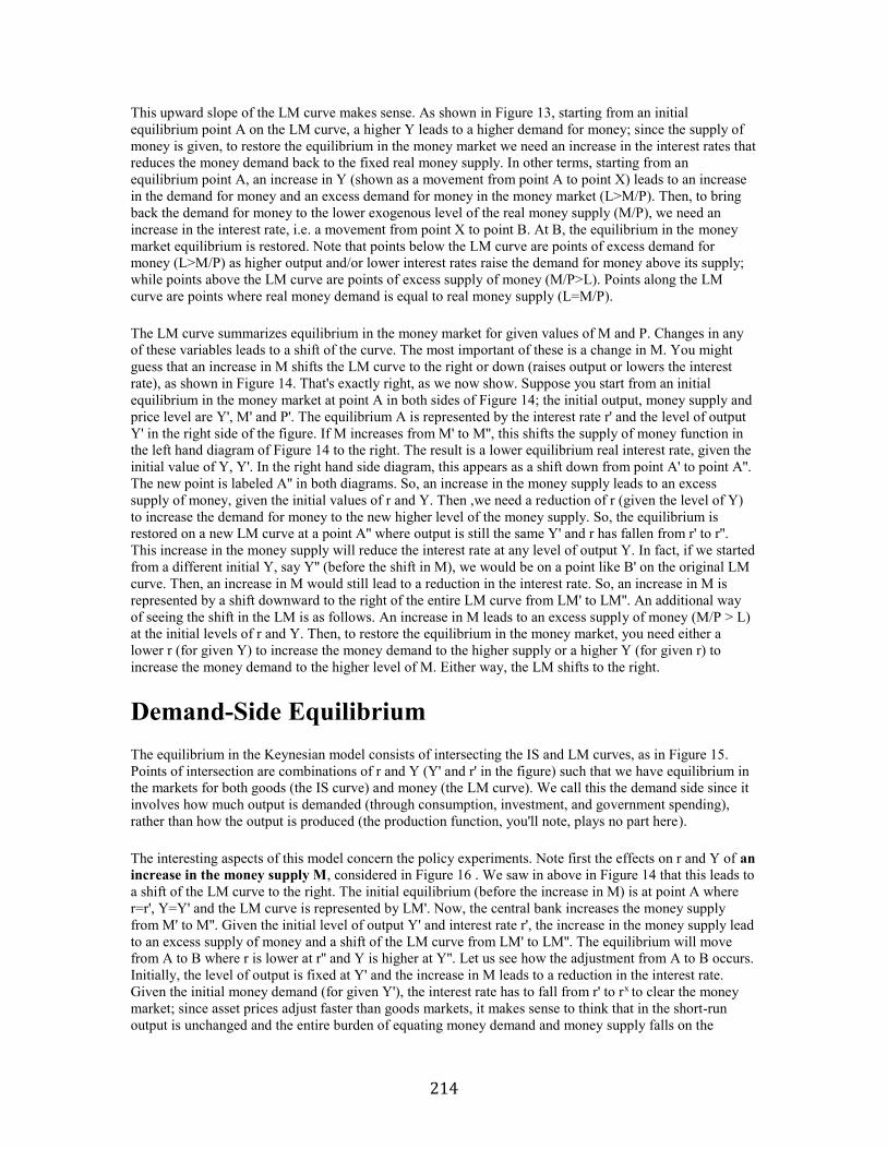
214

This upward slope of the LM curve makes sense. As shown in Figure 13, starting from an initial

equilibrium point A on the LM curve, a higher Y leads to a higher demand for money; since the supply of

money is given, to restore the equilibrium in the money market we need an increase in the interest rates that

reduces the money demand back to the fixed real money supply. In other terms, starting from an

equilibrium point A, an increase in Y (shown as a movement from point A to point X) leads to an increase

in the demand for money and an excess demand for money in the money market (L>M/P). Then, to bring

back the demand for money to the lower exogenous level of the real money supply (M/P), we need an

increase in the interest rate, i.e. a movement from point X to point B. At B, the equilibrium in the money

market equilibrium is restored. Note that points below the LM curve are points of excess demand for

money (L>M/P) as higher output and/or lower interest rates raise the demand for money above its supply;

while points above the LM curve are points of excess supply of money (M/P>L). Points along the LM

curve are points where real money demand is equal to real money supply (L=M/P).

The LM curve summarizes equilibrium in the money market for given values of M and P. Changes in any

of these variables leads to a shift of the curve. The most important of these is a change in M. You might

guess that an increase in M shifts the LM curve to the right or down (raises output or lowers the interest

rate), as shown in Figure 14. That's exactly right, as we now show. Suppose you start from an initial

equilibrium in the money market at point A in both sides of Figure 14; the initial output, money supply and

price level are Y', M' and P'. The equilibrium A is represented by the interest rate r' and the level of output

Y' in the right side of the figure. If M increases from M' to M'', this shifts the supply of money function in

the left hand diagram of Figure 14 to the right. The result is a lower equilibrium real interest rate, given the

initial value of Y, Y'. In the right hand side diagram, this appears as a shift down from point A' to point A''.

The new point is labeled A'' in both diagrams. So, an increase in the money supply leads to an excess

supply of money, given the initial values of r and Y. Then ,we need a reduction of r (given the level of Y)

to increase the demand for money to the new higher level of the money supply. So, the equilibrium is

restored on a new LM curve at a point A'' where output is still the same Y' and r has fallen from r' to r''.

This increase in the money supply will reduce the interest rate at any level of output Y. In fact, if we started

from a different initial Y, say Y'' (before the shift in M), we would be on a point like B' on the original LM

curve. Then, an increase in M would still lead to a reduction in the interest rate. So, an increase in M is

represented by a shift downward to the right of the entire LM curve from LM' to LM''. An additional way

of seeing the shift in the LM is as follows. An increase in M leads to an excess supply of money (M/P > L)

at the initial levels of r and Y. Then, to restore the equilibrium in the money market, you need either a

lower r (for given Y) to increase the money demand to the higher supply or a higher Y (for given r) to

increase the money demand to the higher level of M. Either way, the LM shifts to the right.

Demand-Side Equilibrium

The equilibrium in the Keynesian model consists of intersecting the IS and LM curves, as in Figure 15.

Points of intersection are combinations of r and Y (Y' and r' in the figure) such that we have equilibrium in

the markets for both goods (the IS curve) and money (the LM curve). We call this the demand side since it

involves how much output is demanded (through consumption, investment, and government spending),

rather than how the output is produced (the production function, you'll note, plays no part here).

The interesting aspects of this model concern the policy experiments. Note first the effects on r and Y of an

increase in the money supply M, considered in Figure 16 . We saw in above in Figure 14 that this leads to

a shift of the LM curve to the right. The initial equilibrium (before the increase in M) is at point A where

r=r', Y=Y' and the LM curve is represented by LM'. Now, the central bank increases the money supply

from M' to M''. Given the initial level of output Y' and interest rate r', the increase in the money supply lead

to an excess supply of money and a shift of the LM curve from LM' to LM''. The equilibrium will move

from A to B where r is lower at r'' and Y is higher at Y''. Let us see how the adjustment from A to B occurs.

Initially, the level of output is fixed at Y' and the increase in M leads to a reduction in the interest rate.

Given the initial money demand (for given Y'), the interest rate has to fall from r' to rx to clear the money

market; since asset prices adjust faster than goods markets, it makes sense to think that in the short-run

output is unchanged and the entire burden of equating money demand and money supply falls on the

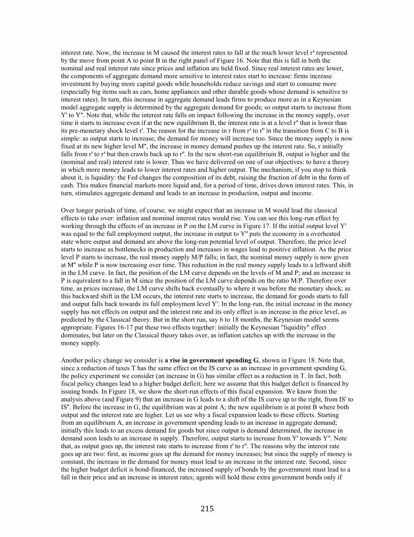
215

interest rate. Now, the increase in M caused the interest rates to fall at the much lower level rx represented

by the move from point A to point B in the right panel of Figure 16. Note that this is fall in both the

nominal and real interest rate since prices and inflation are held fixed. Since real interest rates are lower,

the components of aggregate demand more sensitive to interest rates start to increase: firms increase

investment by buying more capital goods while households reduce savings and start to consume more

(especially big items such as cars, home appliances and other durable goods whose demand is sensitive to

interest rates). In turn, this increase in aggregate demand leads firms to produce more as in a Keynesian

model aggregate supply is determined by the aggregate demand for goods; so output starts to increase from

Y' to Y''. Note that, while the interest rate falls on impact following the increase in the money supply, over

time it starts to increase even if at the new equilibrium B, the interest rate is at a level r'' that is lower than

its pre-monetary shock level r'. The reason for the increase in r from rx to r'' in the transition from C to B is

simple: as output starts to increase, the demand for money will increase too. Since the money supply is now

fixed at its new higher level M'', the increase in money demand pushes up the interest rate. So, r initially

falls from r' to rx but then crawls back up to r''. In the new short-run equilibrium B, output is higher and the

(nominal and real) interest rate is lower. Thus we have delivered on one of our objectives: to have a theory

in which more money leads to lower interest rates and higher output. The mechanism, if you stop to think

about it, is liquidity: the Fed changes the composition of its debt, raising the fraction of debt in the form of

cash. This makes financial markets more liquid and, for a period of time, drives down interest rates. This, in

turn, stimulates aggregate demand and leads to an increase in production, output and income.

Over longer periods of time, of course, we might expect that an increase in M would lead the classical

effects to take over: inflation and nominal interest rates would rise. You can see this long-run effect by

working through the effects of an increase in P on the LM curve in Figure 17. If the initial output level Y'

was equal to the full employment output, the increase in output to Y'' puts the economy in a overheated

state where output and demand are above the long-run potential level of output. Therefore, the price level

starts to increase as bottlenecks in production and increases in wages lead to positive inflation. As the price

level P starts to increase, the real money supply M/P falls; in fact, the nominal money supply is now given

at M'' while P is now increasing over time. This reduction in the real money supply leads to a leftward shift

in the LM curve. In fact, the position of the LM curve depends on the levels of M and P; and an increase in

P is equivalent to a fall in M since the position of the LM curve depends on the ratio M/P. Therefore over

time, as prices increase, the LM curve shifts back eventually to where it was before the monetary shock; as

this backward shift in the LM occurs, the interest rate starts to increase, the demand for goods starts to fall

and output falls back towards its full employment level Y'. In the long-run, the initial increase in the money

supply has not effects on output and the interest rate and its only effect is an increase in the price level, as

predicted by the Classical theory. But in the short run, say 6 to 18 months, the Keynesian model seems

appropriate. Figures 16-17 put these two effects together: initially the Keynesian "liquidity" effect

dominates, but later on the Classical theory takes over, as inflation catches up with the increase in the

money supply.

Another policy change we consider is a rise in government spending G, shown in Figure 18. Note that,

since a reduction of taxes T has the same effect on the IS curve as an increase in government spending G,

the policy experiment we consider (an increase in G) has similar effect as a reduction in T. In fact, both

fiscal policy changes lead to a higher budget deficit; here we assume that this budget deficit is financed by

issuing bonds. In Figure 18, we show the short-run effects of this fiscal expansion. We know from the

analysis above (and Figure 9) that an increase in G leads to a shift of the IS curve up to the right, from IS' to

IS''. Before the increase in G, the equilibrium was at point A; the new equilibrium is at point B where both

output and the interest rate are higher. Let us see why a fiscal expansion leads to these effects. Starting

from an equilibrium A, an increase in government spending leads to an increase in aggregate demand;

initially this leads to an excess demand for goods but since output is demand determined, the increase in

demand soon leads to an increase in supply. Therefore, output starts to increase from Y' towards Y''. Note

that, as output goes up, the interest rate starts to increase from r' to r''. The reasons why the interest rate

goes up are two: first, as income goes up the demand for money increases; but since the supply of money is

constant, the increase in the demand for money must lead to an increase in the interest rate. Second, since

the higher budget deficit is bond-financed, the increased supply of bonds by the government must lead to a

fall in their price and an increase in interest rates; agents will hold these extra government bonds only if

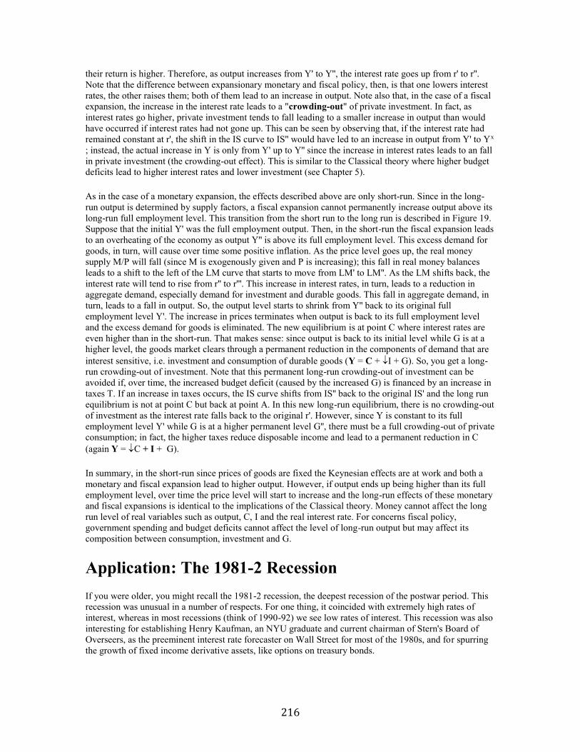
216

their return is higher. Therefore, as output increases from Y' to Y'', the interest rate goes up from r' to r''.

Note that the difference between expansionary monetary and fiscal policy, then, is that one lowers interest

rates, the other raises them; both of them lead to an increase in output. Note also that, in the case of a fiscal

expansion, the increase in the interest rate leads to a "crowding-out" of private investment. In fact, as

interest rates go higher, private investment tends to fall leading to a smaller increase in output than would

have occurred if interest rates had not gone up. This can be seen by observing that, if the interest rate had

remained constant at r', the shift in the IS curve to IS'' would have led to an increase in output from Y' to Yx

; instead, the actual increase in Y is only from Y' up to Y'' since the increase in interest rates leads to an fall

in private investment (the crowding-out effect). This is similar to the Classical theory where higher budget

deficits lead to higher interest rates and lower investment (see Chapter 5).

As in the case of a monetary expansion, the effects described above are only short-run. Since in the long-

run output is determined by supply factors, a fiscal expansion cannot permanently increase output above its

long-run full employment level. This transition from the short run to the long run is described in Figure 19.

Suppose that the initial Y' was the full employment output. Then, in the short-run the fiscal expansion leads

to an overheating of the economy as output Y'' is above its full employment level. This excess demand for

goods, in turn, will cause over time some positive inflation. As the price level goes up, the real money

supply M/P will fall (since M is exogenously given and P is increasing); this fall in real money balances

leads to a shift to the left of the LM curve that starts to move from LM' to LM''. As the LM shifts back, the

interest rate will tend to rise from r'' to r'''. This increase in interest rates, in turn, leads to a reduction in

aggregate demand, especially demand for investment and durable goods. This fall in aggregate demand, in

turn, leads to a fall in output. So, the output level starts to shrink from Y'' back to its original full

employment level Y'. The increase in prices terminates when output is back to its full employment level

and the excess demand for goods is eliminated. The new equilibrium is at point C where interest rates are

even higher than in the short-run. That makes sense: since output is back to its initial level while G is at a

higher level, the goods market clears through a permanent reduction in the components of demand that are

interest sensitive, i.e. investment and consumption of durable goods (Y = C + I + G). So, you get a long-

run crowding-out of investment. Note that this permanent long-run crowding-out of investment can be

avoided if, over time, the increased budget deficit (caused by the increased G) is financed by an increase in

taxes T. If an increase in taxes occurs, the IS curve shifts from IS'' back to the original IS' and the long run

equilibrium is not at point C but back at point A. In this new long-run equilibrium, there is no crowding-out

of investment as the interest rate falls back to the original r'. However, since Y is constant to its full

employment level Y' while G is at a higher permanent level G'', there must be a full crowding-out of private

consumption; in fact, the higher taxes reduce disposable income and lead to a permanent reduction in C

(again Y = C + I + G).

In summary, in the short-run since prices of goods are fixed the Keynesian effects are at work and both a

monetary and fiscal expansion lead to higher output. However, if output ends up being higher than its full

employment level, over time the price level will start to increase and the long-run effects of these monetary

and fiscal expansions is identical to the implications of the Classical theory. Money cannot affect the long

run level of real variables such as output, C, I and the real interest rate. For concerns fiscal policy,

government spending and budget deficits cannot affect the level of long-run output but may affect its

composition between consumption, investment and G.

Application: The 1981-2 Recession

If you were older, you might recall the 1981-2 recession, the deepest recession of the postwar period. This

recession was unusual in a number of respects. For one thing, it coincided with extremely high rates of

interest, whereas in most recessions (think of 1990-92) we see low rates of interest. This recession was also

interesting for establishing Henry Kaufman, an NYU graduate and current chairman of Stern's Board of

Overseers, as the preeminent interest rate forecaster on Wall Street for most of the 1980s, and for spurring

the growth of fixed income derivative assets, like options on treasury bonds.

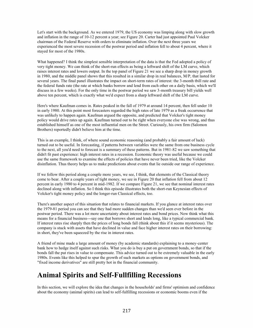
217

Let's start with the background. As we entered 1979, the US economy was limping along with slow growth

and inflation in the range of 10-12 percent a year; see Figure 20. Carter had just appointed Paul Volcker

chairman of the Federal Reserve with orders to eliminate inflation. Over the next three years we

experienced the most severe recession of the postwar period and inflation fell to about 4 percent, where it

stayed for most of the 1980s.

What happened? I think the simplest sensible interpretation of the data is that the Fed adopted a policy of

very tight money. We can think of the short-run effects as being a leftward shift of the LM curve, which

raises interest rates and lowers output. In the top panel of Figure 21 we see a sharp drop in money growth

in 1980, and the middle panel shows that this resulted in a similar drop in real balances, M/P, that lasted for

several years. The final panel illustrates the impact on short-term rates of interest: the 3-month tbill rate and

the federal funds rate (the rate at which banks borrow and lend from each other on a daily basis, which we'll

discuss in a few weeks). For the only time in the postwar period we saw 3-month treasury bill yields well

above ten percent, which is exactly what we'd expect from a sharp leftward shift of the LM curve.

Here's where Kaufman comes in. Rates peaked in the fall of 1979 at around 14 percent, then fell under 10

in early 1980. At this point most forecasters regarded the high rates of late 1979 as a freak occurrence that

was unlikely to happen again. Kaufman argued the opposite, and predicted that Volcker's tight money

policy would drive rates up again. Kaufman turned out to be right when everyone else was wrong, and thus

established himself as one of the most influential men on the Street. Curiously, his own firm (Salomon

Brothers) reportedly didn't believe him at the time.

This is an example, I think, of where sound economic reasoning (and probably a fair amount of luck)

turned out to be useful. In forecasting, if patterns between variables were the same from one business cycle

to the next, all you'd need to forecast is a summary of these patterns. But in 1981-82 we saw something that

didn't fit past experience: high interest rates in a recession. Economic theory was useful because we could

use the same framework to examine the effects of policies that have never been tried, like the Volcker

disinflation. Thus theory helps us to make predictions about events that lie outside our range of experience.

If we follow this period along a couple more years, we see, I think, that elements of the Classical theory

come to bear. After a couple years of tight money, we see in Figure 20 that inflation fell from about 12

percent in early 1980 to 4 percent in mid-1982. If we compare Figure 21, we see that nominal interest rates

declined along with inflation. So I think this episode illustrates both the short-run Keynesian effects of

Volcker's tight money policy and the longer-run Classical effects, too.

There's another aspect of this situation that relates to financial markets. If you glance at interest rates over

the 1979-81 period you can see that they had more sudden changes than we'd seen ever before in the

postwar period. There was a lot more uncertainty about interest rates and bond prices. Now think what this

means for a financial business---say one that borrows short and lends long, like a typical commercial bank.

If interest rates rise sharply then the prices of long bonds fall (think about this if it seems mysterious). The

company is stuck with assets that have declined in value and face higher interest rates on their borrowing:

in short, they've been squeezed by the rise in interest rates.

A friend of mine made a large amount of money (by academic standards) explaining to a money-center

bank how to hedge itself against such risks. What you do is buy a put on government bonds, so that if the

bonds fall the put rises in value to compensate. This advice turned out to be extremely valuable in the early

1980s. Events like this helped to spur the growth of such markets as options on government bonds, and

"fixed income derivatives" are still pretty hot in the financial community.

Animal Spirits and Self-Fullfilling Recessions

In this section, we will explore the idea that changes in the households' and firms' optimism and confidence

about the economy (animal spirits) can lead to self-fulfilling recessions or economic booms even if the

218

fundamental determinants of income and interest rates have not changes. Suppose that suddenly households

and firms become more pessimistic about the future of the economy. This change is the market mood or

confidence may occur even if there has been no change in the current fundamentals. For example,

households may start to cut consumption even if the the level of their disposable income is unchanged and

the level of interest rate is unchanged. This reduction in consumption (in spite of the constancy of the

determinants of consumption, disposable income and interest rates) may occur if there is an event that

makes households more pessimistic about their future income. For example, when Iraq invaded Kuwait in

the summer of 1990, the U.S. economy started to go into a recession. Why ? Part of the story is that

households were nervous about the future effects of the invasion on the economy and started to cut their

consumption spending in spite of the fact that their current incomes and interest rates were unchanged. This

exogenous reduction in consumption led to a fall in aggregate demand; in turn, this fall in aggregate

demand led to a fall in production that resulted in the recession of 1991-1992. In other terms, an exogenous

change in consumer confidence about the future of the economy led to a self-fullfilling recession.

Households started to consume less because they were worried about their future income; according to the

conventional lore, in 1990-91 people were staying at home and following the Kuwait crisis on CNN rather

than going out and spending their incomes. In turn, this initial concern about future incomes led to a fall in

consumption that caused the recession that was being feared in the first place. Similar changes in optimism,

investors's mood (otherwise called by Keynes "animal spirits") and consumer confidence may lead to

changes in the firms' investment demand even if fundamental determinants of investment (such as real

interest rates) have not changed. Firms may suddenly become concerned about the future of the economy

and this change in firms' animal spirits may or may not be related to actual changes in the current state of

the economy. If this change in firms' sentiment occurs, they may start to cut their investment (their

purchases of plant and equipment). This fall in investment demand, in turn, leads to a fall in aggregate

demand and a self-fullfilling fall in output. I.e. a recession may end up occurring just because consumers

and firms start to believe that a recession might be occurring in the future.

How can we formalize the idea of self-fullfilling changes in output due to animal spirits in the context of

out IS/LM model? You remember that when we derived above the consumption and investment demand

functions we said that these functions depend on fundamental variables such as Y-T and r for consumption

and r for investment. However, we also argued that there are some components of consumption and

investment that are exogenous and we called such autonomous components c0 and i0; these autonomous

components of aggregate demand are those that are affected by animal spirits as they lead to changes in C

or I even if there are no changes in fundamentals (Y-T or r). Formally, the consumption and investment

functions are:

C = c0+ b (Y-T) - a r

I = i0- d r

Lets us then consider the effects on the IS curve of exogenous changes in the autonomous components of

consumption and investment. A reduction in either c0 or i0 represents a reduction in some exogenous

component of aggregate demand. Therefore, if initially the economy was in equilibrium, such exogenous

fall in demand is exactly equivalent to other types of exogenous reductions in aggregate demand, such as an

exogenous fall in government spending G. We know from the previous analysis that a fall in government

spending leads to a shift of the IS curve down to the left. Therefore, an exogenous change in the

autonomous components of consumption or investment (due to animal spirits) will also be represented by

an exogenous shift downward to the left of the IS curve. This case of a recession caused by animal spirits is

then described in Figure 22. Before the change in the investors' and consumers' mood, the equilibrium is at

point A where output is at Y' and the interest rate is at r'. Then, an increase in agents' pessimism about the

economy leads to a fall in exogenous demand even if the fundamentals Y and r are still unchanged; in turn,

this leads to a shift to the left of the IS curve from IS' to IS''. This fall in aggregate demand then leads to a

fall in output/income as firms start to cut production in response to the fall in demand. The ensuing fall in

income further reduces aggregate demand and exacerbates the initial fall in output. The economy starts to

contract and output falls from Y' to Y''. As output falls, the interest rate falls as well: the lower investment

219

demand reduces the demand for loans and borrowing pushing down the interest rate. Also, the fall in output

reduces the demand for money and leads, for given supply of money, to a fall in the interest rate. Over time

the economy moves from point A to point B and the economy falls into a recession.

This is in part the story of the 1990-1991 recession. Of course, these changes in animal spirits were not the

sole cause of that recession as monetary policy and external shocks played also an important role.

However, the discussion above suggests that animal spirits can play a role in the observed business cycles

in the economy. An exogenous increase in optimism (higher consumer and firms' confidence) can lead an

economy out of a recession; conversely, an exogenous fall in consumer and investors confidence can lead

to a self-fullfilling contraction in economic activity. A recession may occur just because many people start

to believe that it may be occurring!

Application: Bolivian Stabilization

Bolivia in the mid-1980s suffered from rates of inflation in excess of 1000 percent per year. On the advice

of Jeffrey Sachs of Harvard, they adopted one of the cleanest examples of an orthodox stabilization: fiscal

budget balance, slower money growth, and market-oriented policies. What we saw was a dramatic fall in

the inflation rate, as you might predict from the Classical theory. We also saw a substantial decline in

output, as the Keynesian theory predicts for the short run. This suggests that the kinds of price inertia we're

talking about are also present at very high rates of inflation (which should tell you why it's so hard to get rid

of inflation once you get it). Sachs remarked on the latter: "When I came, Bolivia was a poor country with

very high inflation. Now Bolivia is simply a poor country."

Application: Is Saving Good for the Economy?

There's an old joke that if you ask twelve economists a question, you get thirteen answers: one from each,

plus two from Keynes. Saving is a good example of this. We saw in the Classical theory that saving was

good for the economy: a high saving rate translated into higher investment, growth in the stock of capital,

and increases in output and wages. This prediction was backed up by data: countries that save the most also

tend to invest the most and grow the fastest.

The Keynesian story is just the opposite. A higher saving rate (the ratio of S to Y) is also a lower

consumption rate, since saving and consumption sum to after-tax income. In terms of the IS/LM diagram,

we can think of an increase in the saving rate as a leftward shift in the IS curve, which (in the theory)

reduces output. The story is that if individuals decide to consume less, this hurts firms, who are trying to

sell, and leads them to lay people off. This is a demand side story in the sense that we are talking about who

demands, or buys, goods, rather than how they are produced. I think the story has some merit.

So who is right? Like our analysis of monetary policy, I think it's a little of both: the Keynesian theory fits

the short term, but over periods longer than a couple years saving clearly raises output (ie, the Classical

theory is the best guide). For example, the short-run effect of a reduction in budget deficits (via a cut in

spending G or an increase in taxes T) may be recessionary according to the Keynesian model; however,

over time, the cut in the budget deficit lead to a fall in real interest rates, less crowding-out and an increase

in private investment. Over time, this increase in investment leads to a larger capital stock and an increase

in potential and actual output. So, while the short run effects of a fiscal contraction may be recessionary,

the long-run effects are likely to be expansionary. This tradeoff between short and long term objectives is

one of the tough issues facing policymakers. On the whole, I tend to worry that short term thinking has led

to policy with poor long term consequences. Businessmen face some of the same problems: when bonuses

are tied to annual performance, there may be little gain to adopting policies with long term benefits.

(Keller, in Rude Awakening, makes this point over and over about the corporate culture at GM.)

Application: Who Should Make Monetary Policy?

220

The Volcker disinflation of 1979-1982, and countless other examples, makes it clear that the short run and

long run effects of monetary policy are much different. In the short run, monetary expansion lowers interest

rates by increasing the level of liquidity in financial markets. In the long run, faster money growth raises

inflation and thus raises nominal interest rates, with no effect on the real rate. Experience suggests that if

the central bank is too closely connected to the government, short run considerations will dominate with

possible adverse consequences in the longer term (unnecessarily high inflation). As a result, many countries

give the central bank some autonomy, much as we do for the judiciary. Eg, US Supreme Court Justices are

appointed for life, and members of the Board of Governors of the Federal Reserve System are appointed for

14 year terms (we'll discuss the Federal Reserve System in more detail later on). This gives elected officials

control, in the longer term, over monetary policy, but insulates monetary policy from day-to-day politics.

Over the last decade or so, there has been increasing pressure in Congress to make the Fed more

"accountable." Articles in the Wall Street Journal and elsewhere note that monetary policy is made by

people who have not been elected, suggesting that perhaps they should be.

Should the Fed be more accountable to Congress? The evidence seems to be that in those countries with

more independent central banks, inflation has been lower and unemployment hasn't been much different. In

this sense, independence may be a good idea. That's generally the recommendation to high inflation

countries: deny the fiscal authority access to the printing presses by making the central bank independent.

The low inflation rates of Germany are surely the result of an extremely independent Bundesbank, which

doesn't seem to have affected them adversely in other respects. German output growth, for example, has

been as good as any European country in the postwar period. It's strange, then, that Congress would then

argue that Fed independence is bad for the US. It's hard, too, to resist a further cheap shot at Congress:

would you rather put monetary policy in the hands of the Greenspan and Co., or the people who brought

you the S&L fiasco?

Summary

1. The central idea of the Keynesian theory is that prices, or inflation rates, have a great deal of

inertia: they do not respond immediately to changes in economic conditions or policy. That allows

monetary policy to influence the real rate of interest and output in the short run.

2. The IS curve summarizes equilibrium in the goods market. It's downward sloping in the diagram.

Increases in G shift it to the right/up. [Write down the equation and draw the graph.]

3. The LM curve summarizes equilibrium in the market for money. It's upward sloping in the

diagram. Increases in M shift it to the right and down. [Write down the equation and draw the

graph.]

4. Equilibrium in the IS/LM model is represented by the intersection of the IS and LM curves.

Increases in G raise Y and r. Increases in M raise Y but lower r.

5. The 1981-2 recession illustrates the impact of monetary policy in the short run, and how elements

of both the Keynesian and Classical theories show up in applications.

6. Stabilizations of hyperinflations suggest that "price inertia" may be relevant there, too.

7. Finally, autonomy of the central bank may improve its performance by insulating it from short

term political pressures.

Copyright: Nouriel Roubini and David Backus, Stern School of Business,

New York University, 1998.

221

Copyright: Nouriel Roubini, Stern School of Business, New York University, 1998.