notes6

1mross/work/coursewk/watres/notes/notes6.bigovh

SECTION VI:

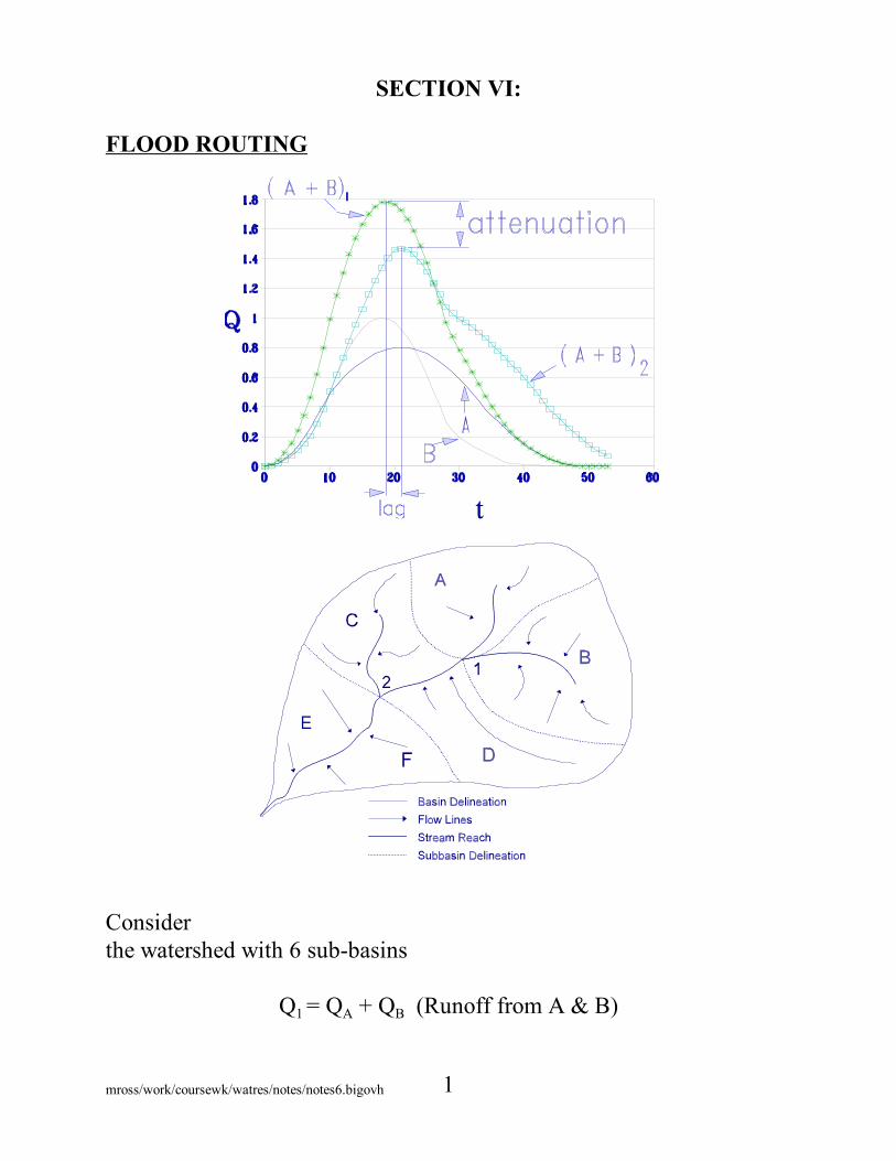
FLOOD ROUTING

Considerthe watershed with 6 sub-basins

Q1 = QA + QB (Runoff from A & B)


Q2 = (QA + QB)2 + QC+ QD(Routed runoff from Q1) + (Direct runoff from C & D)

What causes attenuation? 1) Storage and 2) Friction

What causes flow lag? 1) Flood wave travel time (celerity)- f(length, depth, friction, slope)

Consider a short reach or reservoir (pond)

Continuity Eq.

Qin - Qout = S/ t


See Appendix Figure 4.2 Bedient

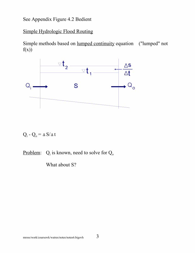
Simple Hydrologic Flood Routing

Simple methods based on lumped continuity equation ("lumped" notf(x))

Qi - Qo = S/ t

Problem: Qi is known, need to solve for Qo

What about S?


To solve the flood routing problem a relationship between S and Q isneeded. Either:

(See handout, USGS rating curve)

2) Q = f(S) or S = f(Q) directly - Less common than (1)

3) Solve for Q(y) from momentum equation(e.g., Q = kym, kinematic ), S(A), A = cross-sectional area


RESERVOIR ROUTING - simplest hydrologic method - sometimescalled "Pond Routing"

"Linear" Reservoir Qo = kS

k = [1/time] = routing coefficient =f (channel geometry)

Qo = outflow linearly related to storage

then Qin - Qout = S/ t

(Homework #’s 4.1, 3, 4, 5, 7)


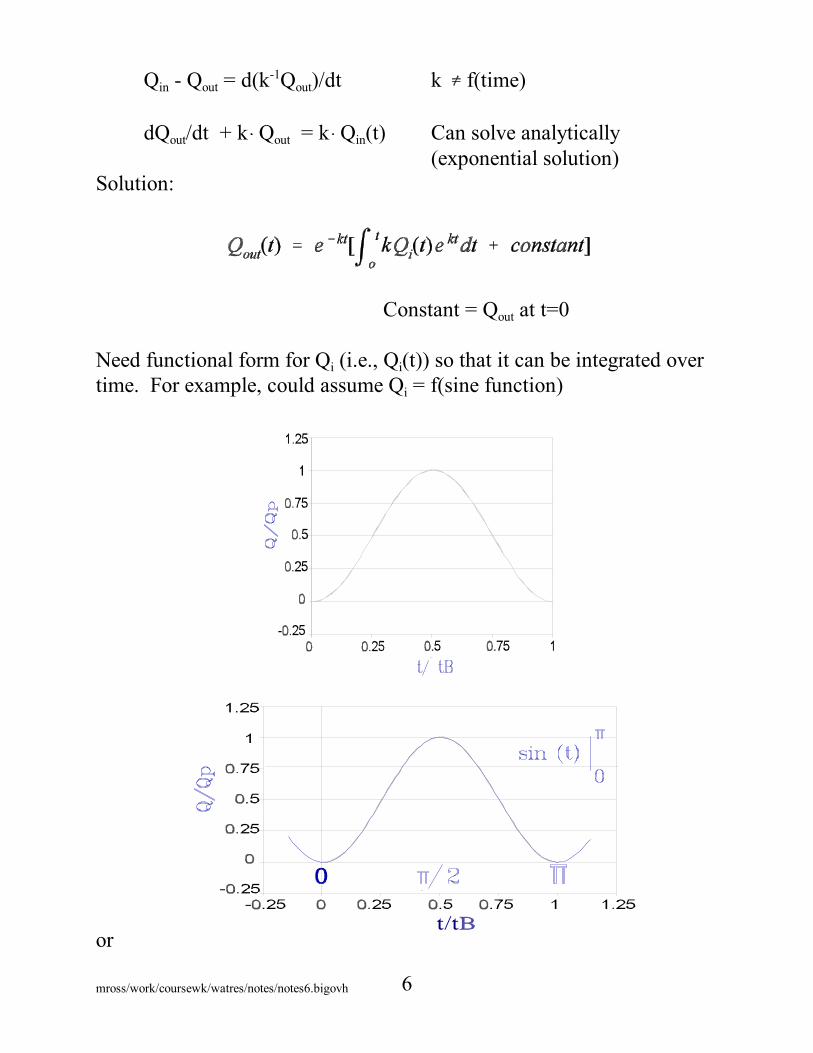
Qin - Qout = d(k-1Qout)/dt k f(time)

dQout/dt + k Qout = k Qin(t) Can solve analytically(exponential solution)

Solution:

Constant = Qout at t=0

Need functional form for Qi (i.e., Qi(t)) so that it can be integrated overtime. For example, could assume Qi = f(sine function)

or


could use numerical (discrete step) methods

Finite Difference Method of Continuity Equation

Qin + Qo = ds/dt

Subscript 1 implies beginning of a time step

Known: Qi1, Qi2, Qo1, S1

Subscript 2 implies end of a time step

Unknown: Qo2, S2


Modified Puls Method (Finite Difference Continuity Eq.)

- also called Storage Indication Method (book)

- collect knowns and unknowns on opposite sides of the equation

To solve: use a relationship between S and Q from rating curve (stage-discharge relation), weir equation, uniform flow assumption, or otherinformation.

Can construct a table or graph of Qo = f(S + ( t/2) Qo)

Book has good example (p. 256 - 260)


Consider a river reach shown

Consider uniform flow


Manning's Equation for uniform flow Seq1 = Sbed

A = cross-sectional areaL = length of channel reachand S = L A = reach storage

Then:

R = Hydraulic radius = Area/ Wetted perimeter

For rectangular channel (y = depth, b = bottom width),

Area = y bWP = 2y + bRh = yb/(2y + b) y/2 for b = 2y

Qo = Constant y2/3 S


Muskingum Method For Flood Routing

S = prism storage + wedge storage = KQo + Kx (Qi - Qo)

Two Parameters K, xx is not distance

Can substitute into continuity


Can solve analytically as before

if x = 0, linear reservoir

In general, 0 x 0.5 note x is higher for more regular("improved") channelsx is lower for more natural channel

e.g., natural irregular channels x ~ 0.15concrete lined, trapezoidal channel 0.3 x 0.4

if x = 0.5, pure translation


Muskingum Eq.

Finite differences applied to continuity Equation

For a linear reservoir x = 0Must have storage and flow data to evaluate parametersPlot graph shown for trial values of x, keep trying with different x, untilloop narrows (approximates a line)

Slope = K , S = K [ x Qi + (1 - x ) Qo]



When storage is a maximum dS/dt = 0 = Qi - Qo, substitute S = K [ Qo + Kx(Qi - Qo)]


If we had these at the same time, we could solve

Use two slope values and solve for x


In the real river reach the parameters are a function of the flow, Q.

For this case need parameter estimation for several flow rates (i.e., variable parameter, K(flow), x(flow), Muskingum Method).

Probably better to just go to full St. Venant (dynamic) equations.

Another method is

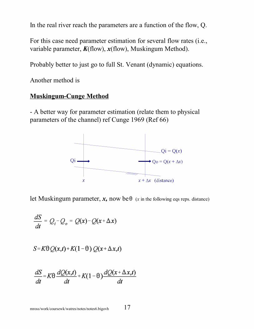
Muskingum-Cunge Method

- A better way for parameter estimation (relate them to physicalparameters of the channel) ref Cunge 1969 (Ref 66)

let Muskingum parameter, x, now be (x in the following eqs reps. distance)


Taylor Series

Remember:

and

Substitute for Q(x + x, t) and dQ(x + x, t)/dt in continuity equation (neglect d3Q/dt dx2 term):

Use continuity equation of the form:

Define:

(Muskingum-Cunge)


Solve for:

LHS

Combine d2Q/dx2 terms:


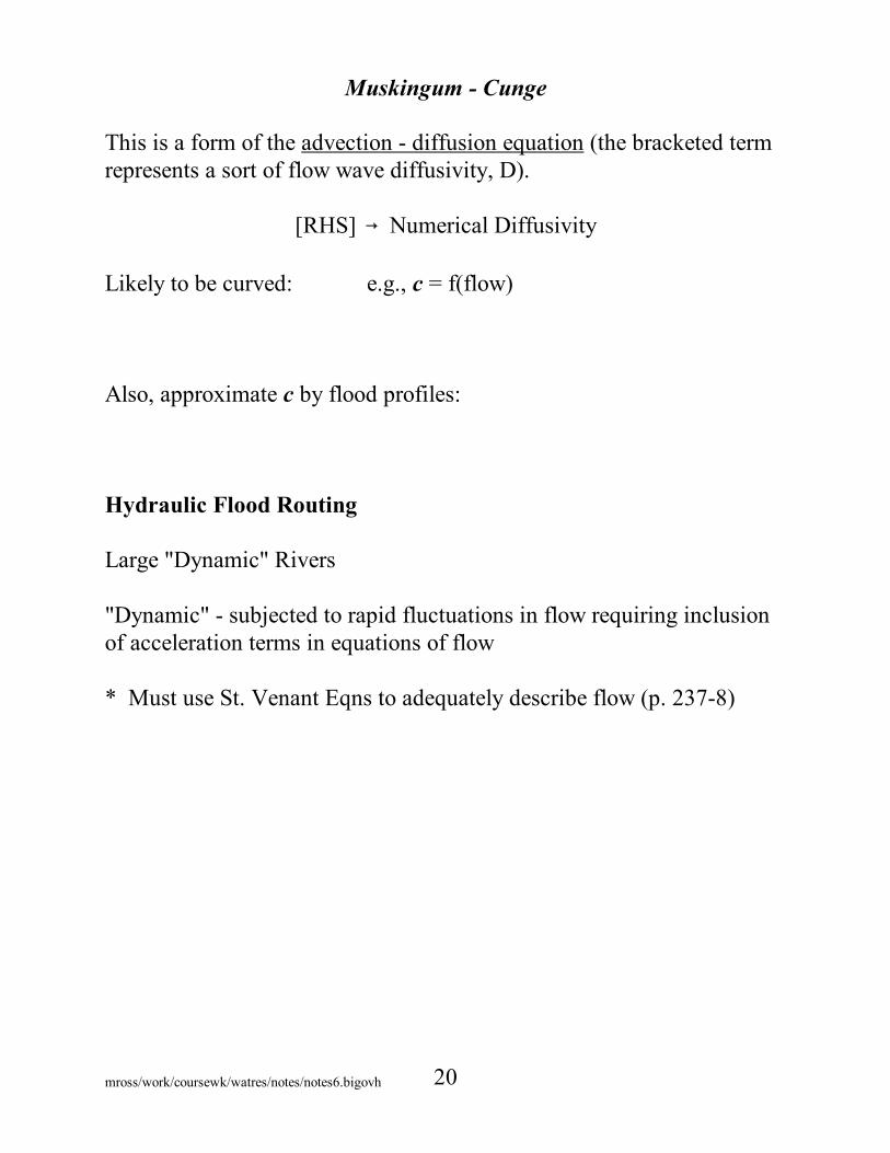
Muskingum - Cunge

This is a form of the advection - diffusion equation (the bracketed termrepresents a sort of flow wave diffusivity, D).

[RHS] Numerical Diffusivity

Likely to be curved: e.g., c = f(flow)

Also, approximate c by flood profiles:

Hydraulic Flood Routing

Large "Dynamic" Rivers

"Dynamic" - subjected to rapid fluctuations in flow requiring inclusionof acceleration terms in equations of flow

* Must use St. Venant Eqns to adequately describe flow (p. 237-8)

Documents

notes6