Embed Size (px)
Citation preview

NOTES ON TIMESERIES ANALYSISARIMA MODELS
AND SIGNALEXTRACTION
Regina Kaiser and Agustín Maravall
Banco de España
Banco de España — Servicio de EstudiosDocumento de Trabajo n.º 0012
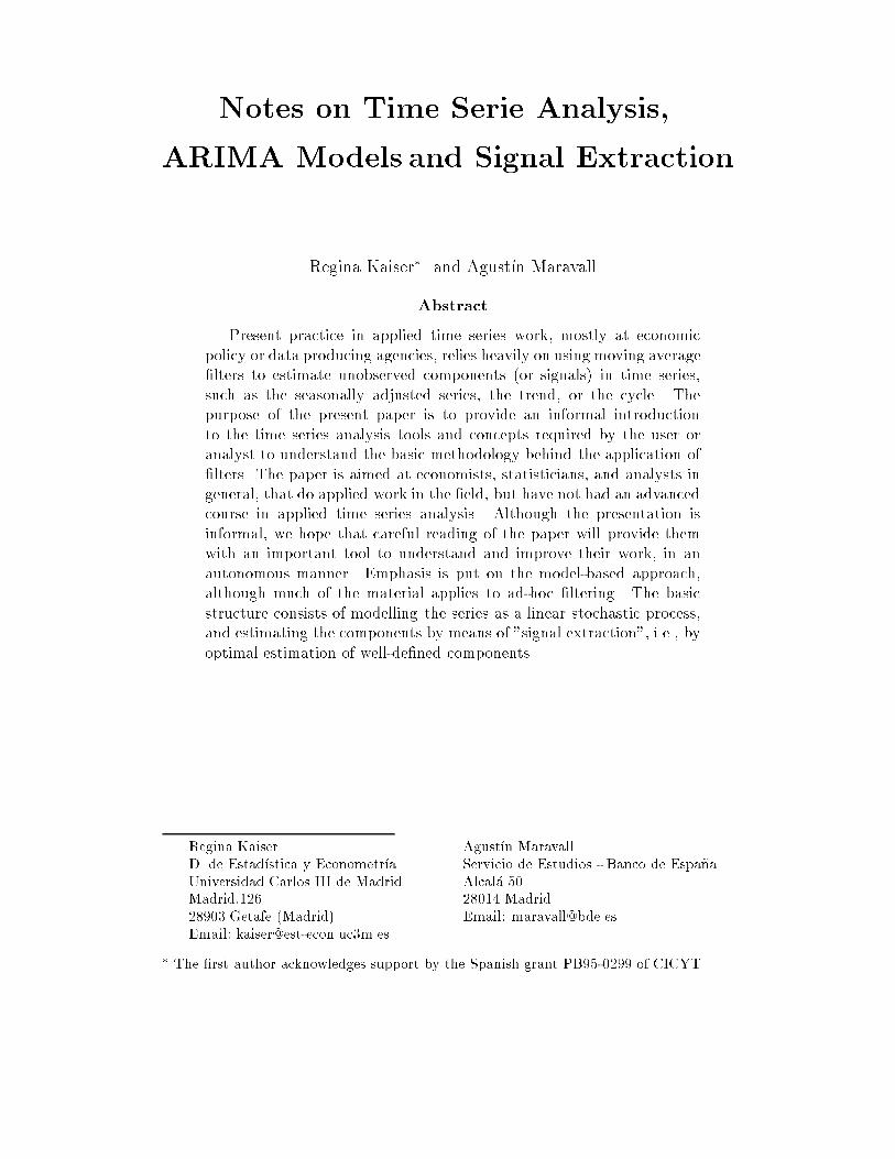
Notes on Time Serie Analysis,
ARIMA Models and Signal Extraction.
Regina Kaiser� and Agust��n Maravall
Abstract
Present practice in applied time series work, mostly at economic
policy or data producing agencies, relies heavily on using moving average
�lters to estimate unobserved components (or signals) in time series,
such as the seasonally adjusted series, the trend, or the cycle. The
purpose of the present paper is to provide an informal introduction
to the time series analysis tools and concepts required by the user or
analyst to understand the basic methodology behind the application of
�lters. The paper is aimed at economists, statisticians, and analysts in
general, that do applied work in the �eld, but have not had an advanced
course in applied time series analysis. Although the presentation is
informal, we hope that careful reading of the paper will provide them
with an important tool to understand and improve their work, in an
autonomous manner. Emphasis is put on the model-based approach,
although much of the material applies to ad-hoc �ltering. The basic
structure consists of modelling the series as a linear stochastic process,
and estimating the components by means of "signal extraction", i.e., by
optimal estimation of well-de�ned components.
Regina Kaiser
D. de Estad��stica y Econometr��a
Universidad Carlos III de Madrid
Madrid,126
28903 Getafe (Madrid)
Email: [email protected]
Agust��n Maravall
Servicio de Estudios - Banco de Espa~na
Alcal�a 50
28014 Madrid
Email: [email protected]
� The �rst author acknowledges support by the Spanish grant PB95-0299 of CICYT
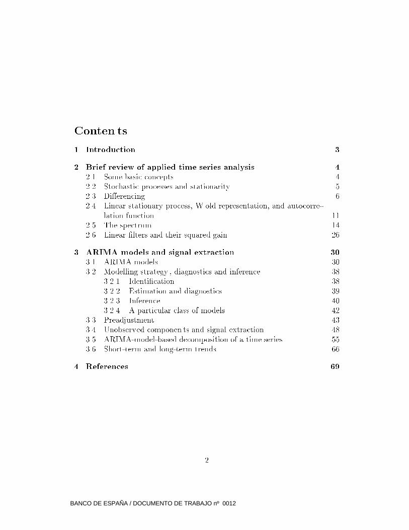
Conten ts
1 Introduction 3
2 Brief review of applied time series analysis 4
2.1 Some basic concepts . . . . . . . . . . . . . . . . . . . . . . . . 4
2.2 Stochastic processes and stationarity . . . . . . . . . . . . . . . 5
2.3 Di�erencing . . . . . . . . . . . . . . . . . . . . . . . . . . . . . 6
2.4 Linear stationary process, W old representation, and autocorre-
lation function . . . . . . . . . . . . . . . . . . . . . . . . . . . . 11
2.5 The spectrum . . . . . . . . . . . . . . . . . . . . . . . . . . . . 14
2.6 Linear �lters and their squared gain . . . . . . . . . . . . . . . . 26
3 ARIMA models and signal extraction 30
3.1 ARIMA models . . . . . . . . . . . . . . . . . . . . . . . . . . . 30
3.2 Modelling strategy , diagnostics and inference . . . . . . . . . . . 38
3.2.1 Identi�cation . . . . . . . . . . . . . . . . . . . . . . . . 38
3.2.2 Estimation and diagnostics . . . . . . . . . . . . . . . . . 39
3.2.3 Inference . . . . . . . . . . . . . . . . . . . . . . . . . . . 40
3.2.4 A particular class of models . . . . . . . . . . . . . . . . 42
3.3 Preadjustment . . . . . . . . . . . . . . . . . . . . . . . . . . . . 43
3.4 Unobserved componen ts and signal extraction . . . . . . . . . . 48
3.5 ARIMA-model-based decomposition of a time series . . . . . . . 55
3.6 Short-term and long-term trends . . . . . . . . . . . . . . . . . 66
4 References 69
2
BANCO DE ESPAÑA / DOCUMENTO DE TRABAJO nº 0012
1 Introduction
Present practice in applied time series w ork, mostly at economic policy or data
producing agencies, relies heavily on using mo ving average �lters to estimate
unobserved componen ts (or signals) in time series. Within the "ad-hoc" �lter-
design approach, well known examples are the X11 �lter for seasonal adjust-
men t, and the Hodrick-Prescott �lter (HP) �lter to estimate business cycles;
see Shiskin et al (1967), and Hodrick and Prescott (1980). Within the "model-
based" approach, whereby the �lters are derived from statistical models, w ell
known examples are the �lters pro vided by programs STAMP and SEA TS;
see Koopman et al. (1996), and Gomez and Maravall (1996). (The program
X12ARIMA can be seen as a move from ad-hoc �ltering towards a partially
model-based approac h; see Findley et al., 1998). The purpose of the present
paper is to provide an informal in troduction to the time series analysis tools
and concepts required by the user or analyst to understand the basic method-
ology behind the application of �lters. The paper is aimed at economists,
statisticians, and analysts in general, that do applied work in the �eld, but
have not had an advanced course in applied time series analysis. Although the
presentation is informal, w e hope that careful reading of the paper will provide
them with an importan t tool to understand and impro ve their work, in an au-
tonomous manner. Emphasis is put on the model-based approach, although
much of the material applies to the ad-hoc �ltering case (in fact, most ad-hoc
�lters can be seen -at least to a close approximation- as particular cases of the
model-based approac h.) The basic structure consists of modelling the series as
a linear stochastic process, and estimating the component by means of "signal
extraction", i.e., by optimal estimation of w ell-de�ned componen ts.
A previous word of caution should be said. The standard �ltering procedure
to estimate business cycles ma y require some prior corrections to the series,
given that otherwise the results can be strongly distorted. An importan t ex-
ample is outlier correction, as w ell as the correction for special e�ects that
can have man y di�erent causes (trading day, easter, or holiday e�ect, legal
changes, modi�cations in the statistical measuremen t procedure, etc.). This
\preadjustemen t" of the series shall be brie y described in Section 3.3, where
references for its methodology and its application in practice will be pro vided,
that also cover the case in which observations are missing. For the rest of the
book, we shall assume that the series either has already been preadjusted, or
that no preadjustmen t is needed.
Further, although the discussion and the approach are also valid for other
frequencies of observation, in order to simplify, we shall concentrate on quar-
terly series.
3
BANCO DE ESPAÑA / DOCUMENTO DE TRABAJO nº 0012
2 Brief review of applied time series analysis
2.1 Some basic concepts
The very basic intuition behind the concept of cyclical or seasonal variation
leads to the idea of decomposing a series in to \unobserved componen ts", mostly
de�ned by the frequency of the associated variation. If xt denotes the observed
series, the simplest form ulation could be
xt =Xj
xjt + ut (2.1)
where the variables xjt denote the unobserved componen ts, and ut a residual
e�ect (often referred to as the \irregular componen t"). In the early days, the
componen ts were often speci�ed to follow deterministic models that could be
estimated b y simple regression. W e shall follow the convention: a Deterministic
Model denotes a model that yields forecasts with zero error when the model
parameters are known. Stochastic Models will pro vide forecasts with non-
zero random errors ev en when the parameters are kno wn. For example, a
deterministic trend component (pt) could be speci�ed as the linear trend
pt = a+ bt; (2.2)
and the seasonal component (st) could be modelled with dummy variables, as
in
st =Xj
cjdjt; (2.3)
where djt = 1 when t corresponds to the jth period of the year, anddjt = 0 oth-
erwise. An equivalent formulation can be expressed in terms of deterministic
sine-cosine functions.
Gradual realization that seasonality evolves in time (an ob vious example
is the weather, one of the basic causes of seasonality) lead to changes in the
estimation procedure. It was found that linear �lters could reproduce the
mo ving features of a trend or a seasonal componen t. A Linear Filter will
simply denote a linear com bination of the seriesxt, as in
yt = c�k1xt�k1 + : : :+ c�1xt�1 + c0xt + c1xt+1 + : : :+ ck2xt+k2 ; (2.4)
and, in so far as yt is then some sort of mo ving average of successive stretches of
xt, we shall also use the expression Mo ving Average (MA) �lter. The w eights
cj could be found in such a way as to capture the relevant variation associated
with the particular component of interest. Thus a �lter for the trend would
capture the variation associated with the long-term mo vement of the series,
and a �lter for a seasonal component would capture variation of a seasonal
4
BANCO DE ESPAÑA / DOCUMENTO DE TRABAJO nº 0012
nature. A �lter designed in this way, with an \a priori" choice of the weights,
is an \ad-hoc" �xed �lter, in the sense that it is independent of the particular
series to which it is being applied. Both, the HP and the X11 �lters can be
seen as "ad-hoc" �xed MA �lters (although, strictly speaking, the coe�cien ts
as we shall see later, will not be constant.)
Over time, however, application of \ad-hoc" �ltering has evidenced some
serious limitations. An importan t one is the fact that, due to its �xed char-
acter, spurious results can be obtained, and for some series the componen t
may be overestimated, while for other series, it ma y be underestimated. To
overcome this limitation, and in the con text of seasonal adjustmen t, an alter-
native approach was suggested (around 1980) whereby the �lter adapted to the
particular structure of the series, as captured by its ARIMA model. The ap-
proach, known as the ARIMA-model-based (AMB) approach, consists of two
steps. First, an ARIMA model is obtained for the observed series. Second,
signal extraction techniques are used to estimate the componen ts with �lters
that are, in some w ell-de�ned way, optimal.
2.2 Stochastic processes and stationarit y
The following summary is an informal review, aimed at providing some basic
tools for the posterior analysis, as well as some in tuition for their usefulness.
More complete treatmen ts of time series analysis are provided in many text-
books; some helpful references are Bo x and Jenkins (1970), Brockwell and
Davis (1987), Granger and Newbold (1986), Harv ey (1993), and Mills (1990).
The starting point is the concept of a Stochastic Process. For our pur-
poses, a stochastic process is a real-valued random variable zt, that follows a
distribution ft(zt), where t denotes an integer that indexes the period. The
T-dimensional v ariable (zt1; zt2; : : : ; ztT ) will have a joint distribution that de-
pends on (t1; t2; : : : ; tT ). A Time Series [zt1; zt2; : : : ; ztT ] will denote a particular
realization of the stochastic process. Thus, for each distribution ft, there is
only one observation available. Not m uch can be learned from this, and more
structure and more assumptions need to be added. T o simplify notation, w e
shall consider the joint distribution of (z1; z2; : : : ; zt), for which a time series is
available when t � T .
From an applied perspectiv e, the two most importan t added assumptions
are
Assumption A: The process is stationary;
Assumption B: The joint distribution of (z1; z2; : : : ; zt) is a multivariate nor-
mal distribution.
5
BANCO DE ESPAÑA / DOCUMENTO DE TRABAJO nº 0012

Assumption A implies the follo wing basic condition. For any value of t,
f(z1; z2; : : : ; zt) = f(z1+k; z2+k; : : : ; zt+k); (2.5)
where k is a integer; that is, the joint distribution remains unc hanged if all
time periods are mo ved a constant number of periods. In particular, letting
t = 1, for the marginal distribution it has to be that
ft(zt) = f(zt)
for every t, and hence the marginal distribution remains constan t. This implies
Ezt = �z ; V zt = Vz (2.6)
where E and V denote the expectation and the variance operators, and�z and
Vz are constants that do not depend on t.
In practice, thus, stationarity implies a constan t mean lev el and bounded
deviations from it. It is a v ery strong requiremen t and few actual economic
series will satisfy it. Its usefulness comes from the fact that relativ ely sim-
ple transformations of the nonstationary series will render it stationary. For
quarterly economic series, it is usually the case that constant variance can be
achieved through the log/level transformation com bined with proper outlier
correction, and constant mean can be ac hieved by di�erencing.
The log transformation is \grosso modo" appropriate when the amplitude
of the series oscillations increases with the level of the series. As for outliers,
several possible types should be considered, the most popular ones being the
additive outlier (i.e., a single spike), the level shift (i.e., a step variable), and
the transitory change (i.e., an e�ect that gradually disappears). Formal test-
ing for the log/level transformation and for outliers are a vailable, as well as
easy-to-apply automatic procedures for doing it (see, for example, G�omez and
Mara vall, 2000a). In Section 3.3 we shall come back to this issue; we center
our attention now on achieving stationarity in mean.
2.3 Di�erencing
Denote by B the backward operator, such that
Bjzt = zt�j (j = 0; 1; 2; : : :);
and let xt denote a quarterly observed series. W e shall use the operators:
� Regular di�erence: r = 1 �B.
� Seasonal di�erence: r4 = 1�B4.
� Annual aggregation: S = 1 +B +B2 +B
3.
6
BANCO DE ESPAÑA / DOCUMENTO DE TRABAJO nº 0012
Thus rxt = xt� xt�1, r4xt = xt � xt�4, and Sxt = xt+ xt�1 + xt�2+ xt�3.
It is imme diately seen that the 3 operators satisfy the identity
r4 = rS (2.7)
If xt is a deterministic linear trend, as in xt = a+ bt, then
rxt = b; (2.8)
r2xt = 0; (2.9)
where r2xt = r(rxt). In general, it can easily be seen that rd will reduce
a polynomial of degree d to a constan t. Obviously, r4xt will also cancel a
constant (or reduce the linear trend to a constant); but it will also cancel
other deterministic periodic functions, suc h as for example, one that repeats
itself every 4 quarters. To �nd the set of functions that are cancelled with
the transformations r4xt, we have to �nd the solution of the homogenous
di�erence equation
r4xt = (1�B4)xt = xt � xt�4 = 0; (2.10)
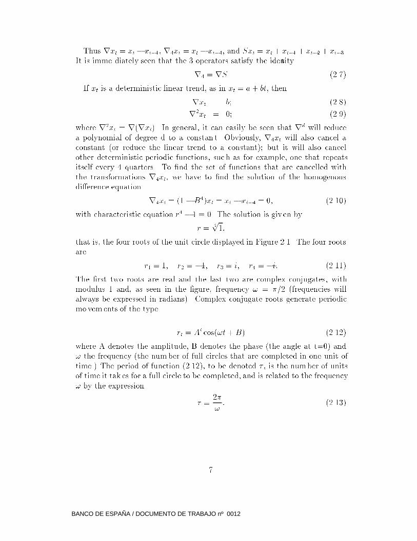
with characteristic equation r4 � 1 = 0. The solution is given by
r =4p1;
that is, the four roots of the unit circle displayed in Figure 2.1. The four roots
are
r1 = 1; r2 = �1; r3 = i; r4 = �i: (2.11)
The �rst two roots are real and the last two are complex conjugates, with
modulus 1 and, as seen in the �gure, frequency ! = �=2 (frequencies will
always be expressed in radians). Complex conjugate roots generate periodic
mo vements of the type
rt = At cos(!t+ B) (2.12)
where A denotes the amplitude, B denotes the phase (the angle at t=0) and
! the frequency (the number of full circles that are completed in one unit of
time.) The period of function (2.12), to be denoted � , is the number of units
of time it tak es for a full circle to be completed, and is related to the frequency
! by the expression
� =2�
!: (2.13)
7
BANCO DE ESPAÑA / DOCUMENTO DE TRABAJO nº 0012
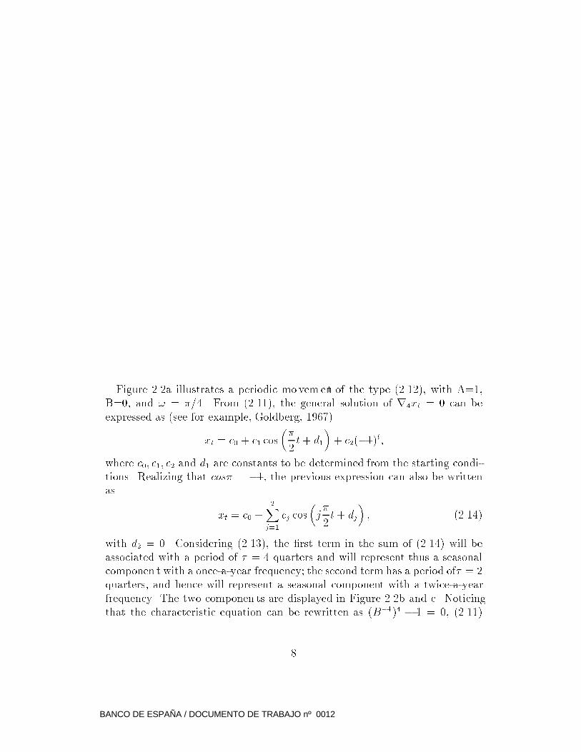
Figure 2.2a illustrates a periodic mo vement of the type (2.12), with A=1,
B=0, and ! = �=4. From (2.11), the general solution of r4xt = 0 can be
expressed as (see for example, Goldberg, 1967)
xt = c0 + c1 cos
��
2t+ d1
�+ c2(�1)t;
where c0; c1; c2 and d1 are constants to be determined from the starting condi-
tions. Realizing that cos� = �1, the previous expression can also be written
as
xt = c0 +2X
j=1
cj cos
�j�
2t+ dj
�; (2.14)
with d2 = 0. Considering (2.13), the �rst term in the sum of (2.14) will be
associated with a period of � = 4 quarters and will represent thus a seasonal
componen t with a once-a-year frequency; the second term has a period of� = 2
quarters, and hence will represent a seasonal component with a twice-a-year
frequency. The two componen ts are displayed in Figure 2.2b and c. Noticing
that the characteristic equation can be rewritten as (B�1)4 � 1 = 0, (2.11)
8
BANCO DE ESPAÑA / DOCUMENTO DE TRABAJO nº 0012
implies the factorization
r4 = (1 �B)(1 +B)(1 +B2):
The factor (1-B) is associated with the constant and the zero frequency, the
factor (1+B) with the t wice-a-year seasonality with frequency! = �, and the
factor (1+B2) with the once-a-year seasonality with frequency ! = �=2. The
product of these last two factors yields the annual aggregation operator S, in
agreemen t with expression (2.7). Hence the transformation Sxt will remo ve
seasonal nonstationarity in xt.
For the most-often-found case in whic h stationarity is achieved through the
di�erencing rr4, the factorization
rr4 = r2S
directly shows that the solution to
rr4xt = 0
will be of the type:
xt = a+ bt+2X
j=1
cj
�cos(j
�
2t) + dj
�; (2.15)
with d2 = 0. Thus the di�erencing will remo ve the same cosine (seasonal)
functions as before, plus the local linear trend (a+bt). For the caser2r4, the
factorization r3S shows that the cancelled trend will now be a second order
polynomial in t, the rest remaining unc hanged. For quarterly series, higher
order di�erencing is never encountered in practice.
A �nal and importan t remark:
� Let D denote, in general, the complete di�erencing applied to the series
xt so as to achieve stationarity. When specifying the ARIMA model for
xt, we shall not be stating that Dxt = 0 (as, for example, in (2.9), ) but
that
Dxt = zt;
where zt is a zero-mean, stationary stoc hastic process with relatively
small variance. Thus every period the solution of Dxt = 0 will be per-
turbed by the stochastic input zt (see Box and Jenkins, 1970, Appendix
A.4.1). In terms of expression (2.15), what this perturbation implies is
that the a,b,c and d coe�cien ts will not be constant but will instead
depend on time. This gradual ev olution of the coe�cien ts provides the
model with an adaptive behavior that will be associated with the \mo v-
ing"features of the trend and seasonal componen ts.
9
BANCO DE ESPAÑA / DOCUMENTO DE TRABAJO nº 0012
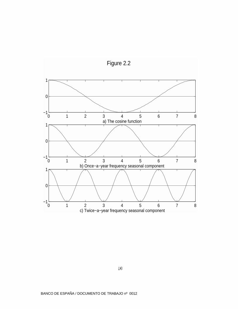
0 1 2 3 4 5 6 7 8−1
0
1
a) The cosine function
0 1 2 3 4 5 6 7 8−1
0
1
b) Once−a−year frequency seasonal component
Figure 2.2
0 1 2 3 4 5 6 7 8−1
0
1
c) Twice−a−year frequency seasonal component
10
BANCO DE ESPAÑA / DOCUMENTO DE TRABAJO nº 0012
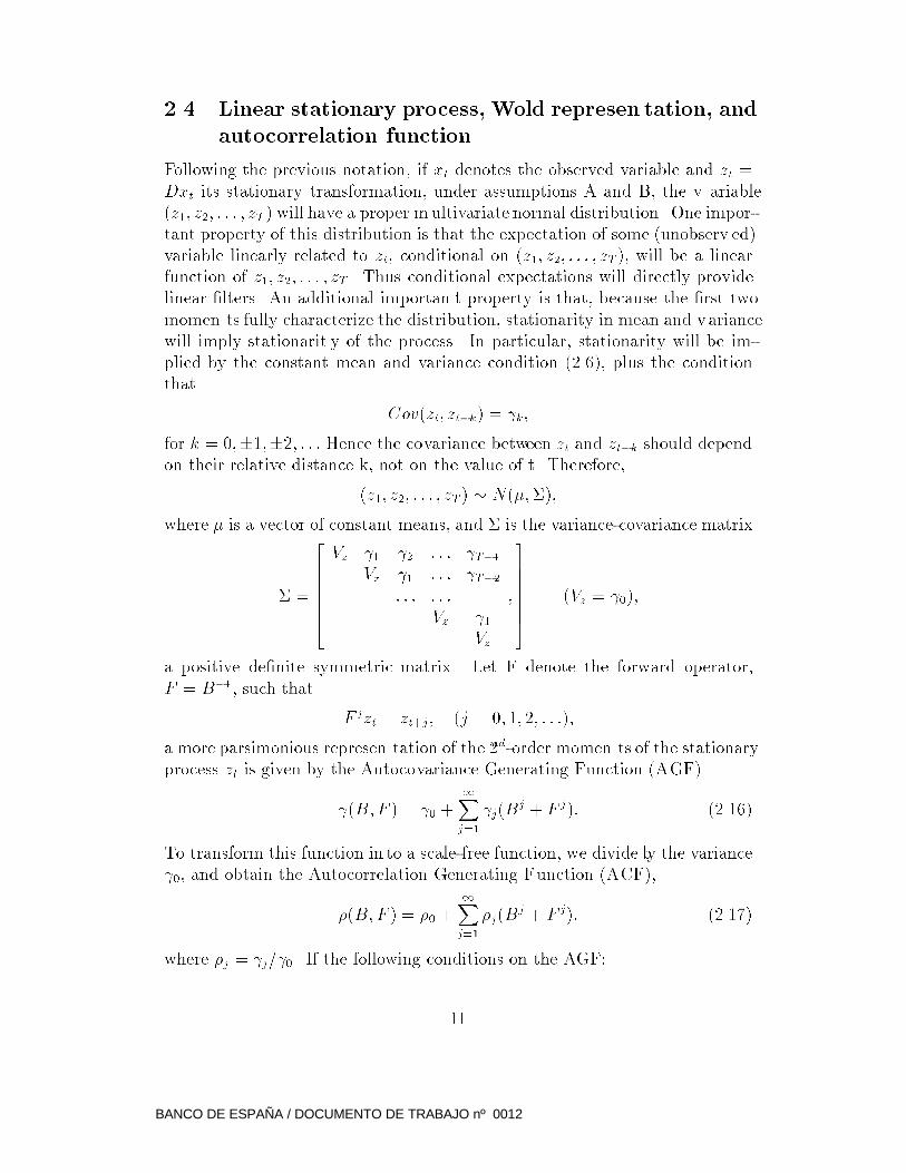
2.4 Linear stationary process, Wold represen tation, and
autocorrelation function
Following the previous notation, if xt denotes the observed variable and zt =
Dxt its stationary transformation, under assumptions A and B, the v ariable
(z1; z2; : : : ; zT ) will have a proper multivariate normal distribution. One impor-
tant property of this distribution is that the expectation of some (unobserv ed)
variable linearly related to zt, conditional on (z1; z2; : : : ; zT ), will be a linear
function of z1; z2; : : : ; zT . Thus conditional expectations will directly provide
linear �lters. An additional importan t property is that, because the �rst two
momen ts fully characterize the distribution, stationarity in mean and variance
will imply stationarit y of the process. In particular, stationarity will be im-
plied by the constant mean and variance condition (2.6), plus the condition
that
Cov(zt; zt�k) = k;
for k = 0;�1;�2; : : : Hence the covariance between zt and zt�k should depend
on their relative distance k, not on the value of t. Therefore,
(z1; z2; : : : ; zT ) � N(�;�);
where � is a vector of constant means, and � is the variance-covariance matrix
� =
26666664
Vz 1 2 : : : T�1
Vz 1 : : : T�2
: : : : : :
Vz 1
Vz
;
37777775
(Vz = 0);
a positive de�nite symmetric matrix. Let F denote the forward operator,
F = B�1, such that
Fjzt = zt+j; (j = 0; 1; 2; : : :);
a more parsimonious represen tation of the 2nd-order momen ts of the stationary
process zt is given by the Autocovariance Generating Function (AGF)
(B;F ) = 0 +1Xj=1
j(Bj + F
j): (2.16)
To transform this function in to a scale-free function, we divide by the variance
0, and obtain the Autocorrelation Generating Function (ACF),
�(B;F ) = �0 +1Xj=1
�j(Bj + F
j): (2.17)
where �j = j= 0. If the following conditions on the AGF:
11
BANCO DE ESPAÑA / DOCUMENTO DE TRABAJO nº 0012
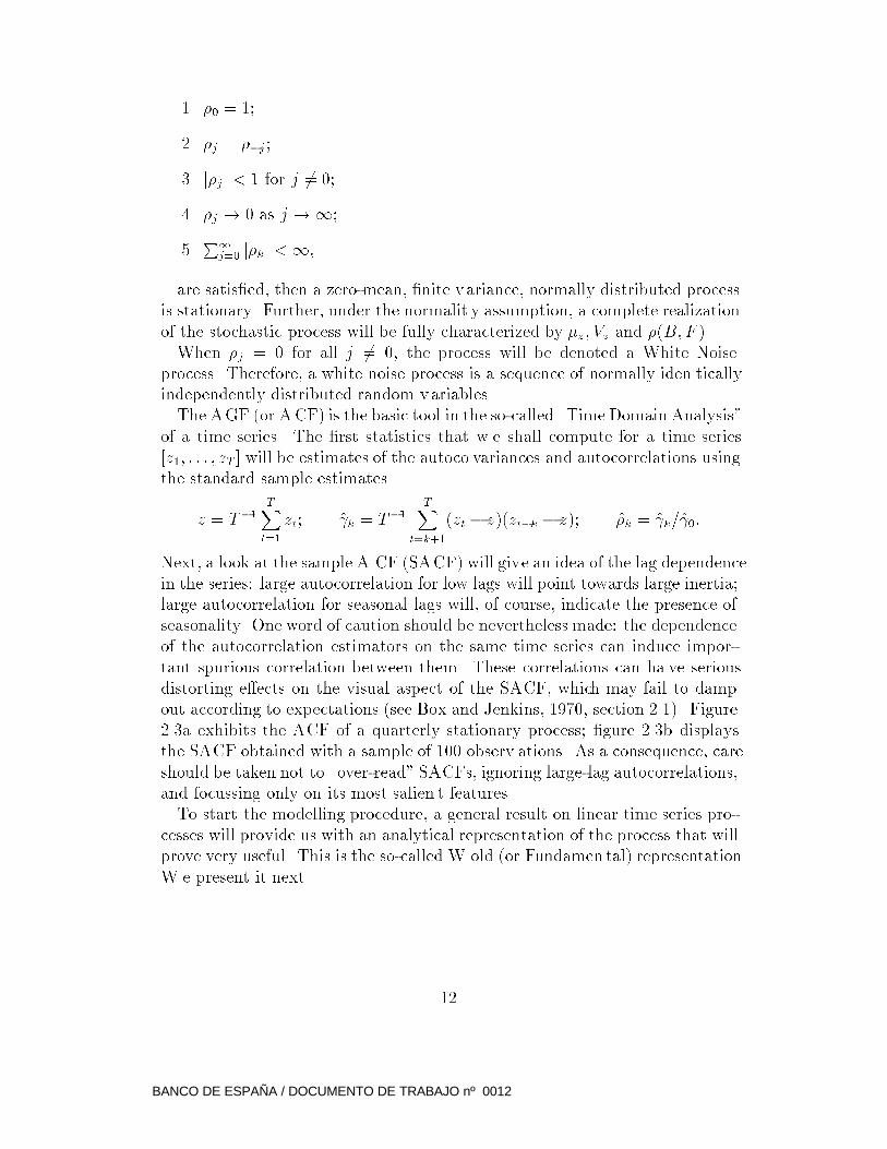
1. �0 = 1;
2. �j = ��j ;
3. j�jj < 1 for j 6= 0;
4. �j ! 0 as j !1;
5.P
1
j=0 j�kj <1,
are satis�ed, then a zero-mean, �nite variance, normally distributed process
is stationary. Further, under the normalit y assumption, a complete realization
of the stochastic process will be fully characterized by �z; Vz and �(B;F ).
When �j = 0 for all j 6= 0, the process will be denoted a White Noise
process. Therefore, a white noise process is a sequence of normally iden tically
independently distributed random variables.
The AGF (or ACF) is the basic tool in the so-called \Time Domain Analysis"
of a time series. The �rst statistics that w e shall compute for a time series
[z1; : : : ; zT ] will be estimates of the autoco variances and autocorrelations using
the standard sample estimates
�z = T�1
TXt=1
zt; k = T�1
TXt=k+1
(zt � �z)(zt�k � �z); �k = k= 0:
Next, a look at the sample A CF (SACF) will give an idea of the lag dependence
in the series: large autocorrelation for low lags will point towards large inertia;
large autocorrelation for seasonal lags will, of course, indicate the presence of
seasonality. One word of caution should be nevertheless made: the dependence
of the autocorrelation estimators on the same time series can induce impor-
tant spurious correlation between them. These correlations can ha ve serious
distorting e�ects on the visual aspect of the SACF, which may fail to damp
out according to expectations (see Box and Jenkins, 1970, section 2.1). Figure
2.3a exhibits the ACF of a quarterly stationary process; �gure 2.3b displays
the SACF obtained with a sample of 100 observ ations. As a consequence, care
should be taken not to \over-read" SACFs, ignoring large-lag autocorrelations,
and focussing only on its most salien t features.
To start the modelling procedure, a general result on linear time series pro-
cesses will provide us with an analytical representation of the process that will
prove very useful. This is the so-called W old (or Fundamen tal) representation.
W e present it next.
12
BANCO DE ESPAÑA / DOCUMENTO DE TRABAJO nº 0012
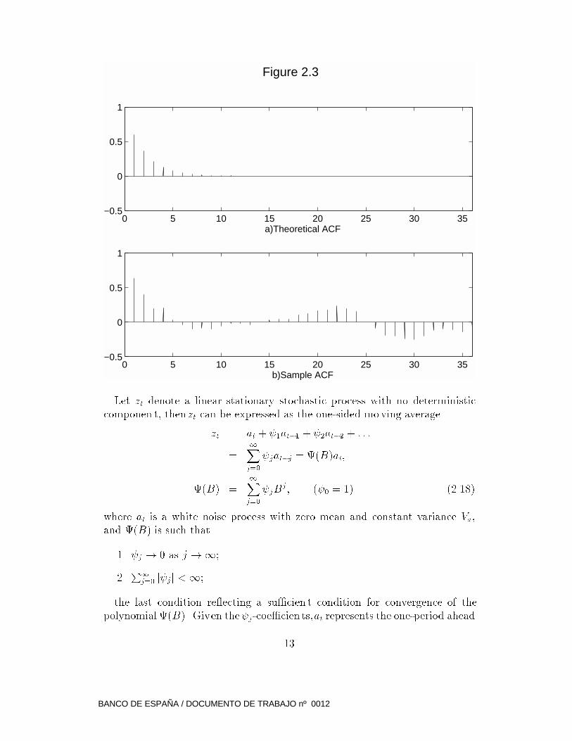
0 5 10 15 20 25 30 35−0.5
0
0.5
1
a)Theoretical ACF
Figure 2.3
0 5 10 15 20 25 30 35−0.5
0
0.5
1
b)Sample ACF
Let zt denote a linear stationary stochastic process with no deterministic
componen t, thenzt can be expressed as the one-sided mo ving average
zt = at + 1at�1 + 2at�2 + : : : =
=1Xj=0
jat�j = (B)at;
(B) =1Xj=0
jBj; ( 0 = 1) (2.18)
where at is a white noise process with zero mean and constant variance Va,
and (B) is such that
1. j ! 0 as j !1;
2.P
1
j=0 j jj <1;
the last condition re ecting a su�cien t condition for convergence of the
polynomial (B). Given the j-coe�cien ts,at represents the one-period ahead
13
BANCO DE ESPAÑA / DOCUMENTO DE TRABAJO nº 0012
forecast error of zt, that is
at = zt � ztjt�1;
where ztjt�1 is the forecast of zt made at period t-1. Since at represents what
is new in zt, that is, what is not contained in its past [zt�1; zt�2; zt�3; : : :], it
will be referred to as the Innovation of the process. The representation of ztin terms of its inno vations, given by (2.18), is unique, and is usually referred
to as the W old representation.
A useful result is the following: If (B;F ) represents the AGF of the process
zt, then
(B;F ) = (B)(F )Va: (2.19)
In particular, for the variance,
Vz = (1 + 21 +
22 + : : :)Va: (2.20)
2.5 The spectrum
The spectrum is the basic tool in the so-called \F requency Domain Approach"
to time series analysis. It represen ts an alternative way to look and interpret
the information con tained in the second-order momen ts of the series. The
frequency approach is particularly convenient for analyzing unobserved com-
ponents, such as trends, cycles, or seasonality. Our aim is not to present a
complete and rigorous description, but to pro vide some in tuition and basic
understanding, that will permit us to use it properly for our purposes. (Tw o
good references for a general presentation are Jenkins and W atts, 1968, and
Grenander and Rosenblatt, 1957.)
Consider, �rst, a time series (i.e., a partial realization of a stoc hastic process)
given by z1; z2; : : : ; zT . To simplify the discussion, assume the process has zero
mean and that T is even, so that we can write T=2q. In the same w ay that,
as is well known, the T values of zt can be exactly duplicated ("explained") by
a polynomial of order (T-1), they can also be exactly reproduced as the sum
of T/2 cosine functions of the type (2.12); this result provides in fact the basis
of Fourier analysis.
Figure 2.4a shows, for example, the quarterly time series of 10 observations
generated by the �ve cosine functions of �gure 2.4b. To construct this set of
functions, we start by de�ning the Fundamental Frequency ! = 2�=T (i.e.,
the frequency of one full circle completed in T periods) and its m ultiples (or
Harmonics)
!j = (2�=T )j; j = 1; 2; : : : ; q:
14
BANCO DE ESPAÑA / DOCUMENTO DE TRABAJO nº 0012
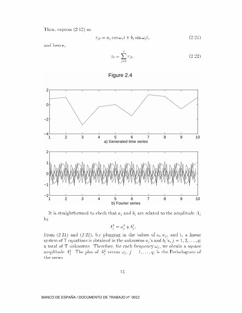
Then, express (2.12) as
rjt = aj cos!jt+ bj sin!jt; (2.21)
and hence,
zt =qX
j=1
rjt: (2.22)
1 2 3 4 5 6 7 8 9 10−4
−2
0
2
a) Generated time series
Figure 2.4
1 2 3 4 5 6 7 8 9 10−2
−1
0
1
2
b) Fourier series
It is straightforward to check that aj and bj are related to the amplitude Aj
by
A2j = a
2j + b
2j :
From (2.21) and (2.22), b y plugging in the values of zt; wj, and t, a linear
system of T equations is obtained in the unknowns aj's and bj's, j = 1; 2; : : : ; q;
a total of T unknowns. Therefore, for each frequency !j , we obtain a square
amplitude A2j . The plot of A2
j versus !j , j = 1; : : : ; q, is the Periodogram of
the series.
15
BANCO DE ESPAÑA / DOCUMENTO DE TRABAJO nº 0012
As a consequence, we obtain a set of periodic functions with di�erent fre-
quencies and amplitudes. W e can group the functions in intervals of frequency
by summing the squared amplitudes of the functions that fall in the same
interval. In this way we obtain an histogram of frequencies that shows the
contribution of each interval of frequency to the series variation; an example
is shown in Figure 2.5a. In the same w ay that a density function is the model
counterpart of the usual histogram, the spectrumwill be the model coun terpart
of the frequency histogram (properly standardized).
0 0.5 1 1.5 2 2.5 30
0.5
1
1.5
2
2.5
3
a) Histogram of frequencies
Figure 2.5
0 0.5 1 1.5 2 2.5 30
0.5
1
1.5
2
2.5
3
b) Power spectrum
W e can now let the interval �!j go to zero, and the frequency histogram
will become a continuous function, which is denoted the Sample Spectrum.
The area over the di�erential d! represents the contribution of the frequencies
in d! to the variation of the time series. An importan t result links the sample
spectrum with the SA CF (see Box and Jenkins, 1970, Appendix A.2.1). If
16
BANCO DE ESPAÑA / DOCUMENTO DE TRABAJO nº 0012
H(!) denotes the sample spectrum, then it is proportional to
H(!) / 0 + 2
T�1Xt=1
j cos!t
!; (2.23)
where j denotes the lag-j autocovariance estimator.
The model equiv alent of (2.23) provides precisely the de�nition of power
spectrum. Consider the A GF of the stationary processzt, given by
(B;F ) = 0 +1Xj=1
j(Bj + F
j); (2.24)
where B is a complex n umber of unit modulus, which can be expressed as
ei!. Replacing B and F by their complex represen tation, (2.24) becomes the
function
g(!) = 0 +1Xj=1
j(e�i!j + e
i!j);
or, using the identity
[e�i!j + ei!j = 2 cos(j!)];
and dividing by 2�, one obtains
g1(!) =1
2�
24 0 + 2
1Xj=1
j cos(j!)
35 : (2.25)
The move from (2.24) to (2.25) is the so-called Fourier cosine transform of the
AGF (B;F ), and is denoted the Power Spectrum. Replacing the A GF by
the ACF (i.e., dividing by the variance 0), we obtain the Spectral Density
Function
g�
1(!) =1
2�
241 + 2
1Xj=1
�j cos(j!)
35 : (2.26)
It is easily seen that g1(!) -or g�
1(!)- are periodic functions, and hence the
range of frequencies can be restricted to (��; �), or (0, 2�). Moreo ver, given
that the cosine function is symmetric around zero, w e only need to consider the
range (0, �). It is worth men tioning that the sample spectrum (2.23), divided
by 2�, is also the Fourier transform of the sample autoco variance function.
From (2.25), knowing the AGF of a process, the power spectrum is trivially
obtained. Alternatively, knowledge of the power spectrum permits us to deriv e
the AGF by means of the in verse Fourier transform, giv en by
k =
Z �
��
g(!) cos(!k)d!:
17
BANCO DE ESPAÑA / DOCUMENTO DE TRABAJO nº 0012
Thus, for k=0,
0 =Z �
��
g(!)d!; (2.27)
which shows that the integral of the power spectrum is the variance of the
process. Therefore, the area under the spectrum for the in terval d! is the
contribution to the variance of the series that corresponds to the range of
frequencies d! (as in Figure 2.5b). Roughly, the power spectrum can be seen
as a decomposition of the variance by frequency.
For the rest of the monograph, in order to simplify the notation, po wer spec-
tra will be expressed in units of 2�, and, because of the symmetry condition,
only the range ! 2 [0; �] will be considered. W e shall refer to this function
simply as the Spectrum.
As an example, consider a process zt, the output of the 2nd-order homogenous
di�erence-equation (deterministic) model
zt + :81zt�2 = 0 (2.28)
The characteristic equation, r2 + :81 = 0 yields the pair of complex conjugate
numbers r = �:9i, situated in the imaginary axis, they will be associated th us
with the frequency ! = �=2 (see Figure 2.1). The process follows therefore the
deterministic function
zt = :9 cos
��
2t+ �
�; (2.29)
where we can set � = ��=2. The function (2.29) does not depend on ! and the
mo vements of zt are all associated with the single frequency ! = �=2. This
explains the isolated spike for that frequency in Figure 2.6a. To transform
the previous model in to a stochastic process, we perturb every period the
equilibrium (2.28) with a white noise (0,1) v ariableat, so that it is replaced
by the stochastic model
zt + :81zt�2 = at; or (1 + :81B2)zt = at: (2.30)
From (2.30), the W old representation (2.18) is imm ediately obtained as
zt =at
1 + :81B2;
with
(B) = 1=(1 + :81B2):
Using (2.19), the AGF of zt can be obtained through
(B;F ) =Va
(1 + :81B2)(1 + :81F 2)=
18
BANCO DE ESPAÑA / DOCUMENTO DE TRABAJO nº 0012
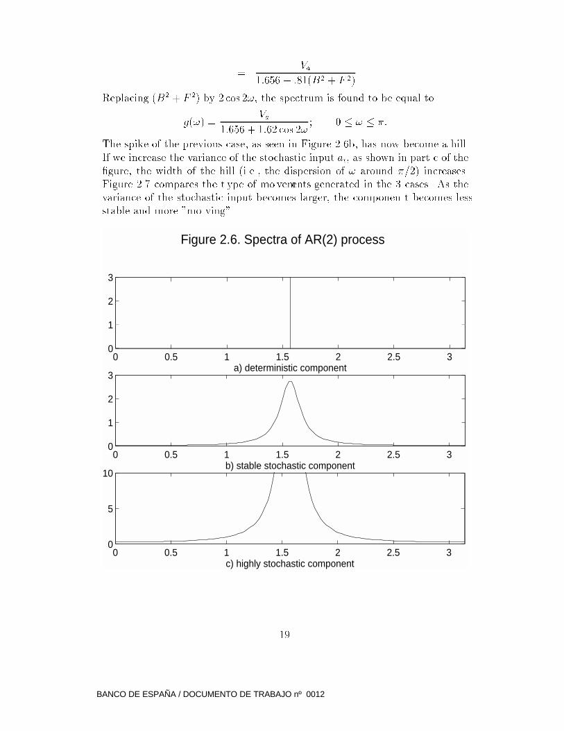
=Va
1:656 + :81(B2 + F 2)
Replacing (B2 + F2) by 2 cos 2!, the spectrum is found to be equal to
g(!) =Va
1:656 + 1:62 cos 2!; 0 � ! � �:
The spike of the previous case, as seen in Figure 2.6b, has now become a hill.
If we increase the variance of the stochastic input at, as shown in part c of the
�gure, the width of the hill (i.e., the dispersion of ! around �=2) increases.
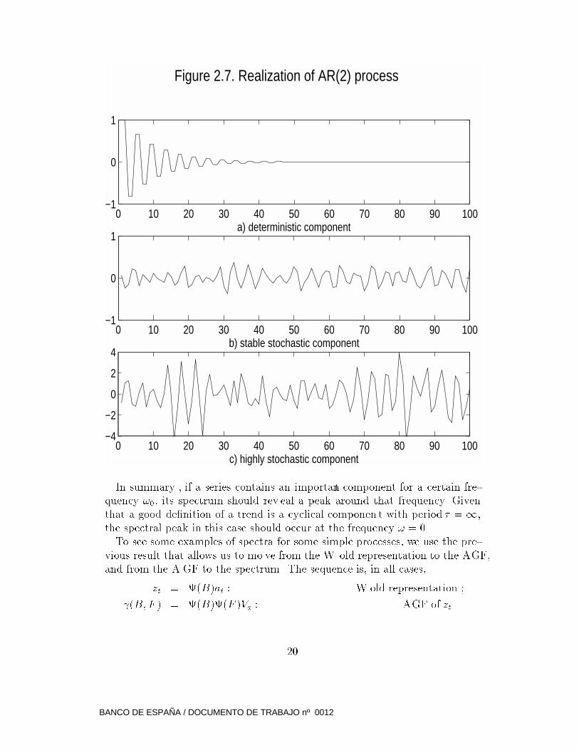
Figure 2.7 compares the t ype of mo vements generated in the 3 cases. As the
variance of the stochastic input becomes larger, the componen t becomes less
stable and more "mo ving".
0 0.5 1 1.5 2 2.5 30
1
2
3
a) deterministic component
0 0.5 1 1.5 2 2.5 30
1
2
3
b) stable stochastic component
Figure 2.6. Spectra of AR(2) process
0 0.5 1 1.5 2 2.5 30
5
10
c) highly stochastic component
19
BANCO DE ESPAÑA / DOCUMENTO DE TRABAJO nº 0012
0 10 20 30 40 50 60 70 80 90 100−1
0
1
a) deterministic component
0 10 20 30 40 50 60 70 80 90 100−1
0
1
b) stable stochastic component
Figure 2.7. Realization of AR(2) process
0 10 20 30 40 50 60 70 80 90 100−4
−2
0
2
4
c) highly stochastic component
In summary , if a series contains an important component for a certain fre-
quency !0, its spectrum should rev eal a peak around that frequency. Given
that a good de�nition of a trend is a cyclical componen t with period � =1,
the spectral peak in this case should occur at the frequency ! = 0.
To see some examples of spectra for some simple processes, we use the pre-
vious result that allows us to mo ve from the W old representation to the AGF,
and from the A GF to the spectrum. The sequence is, in all cases,
zt = (B)at : W old representation ;
(B;F ) = (B)(F )Va : AGF of zt
20
BANCO DE ESPAÑA / DOCUMENTO DE TRABAJO nº 0012
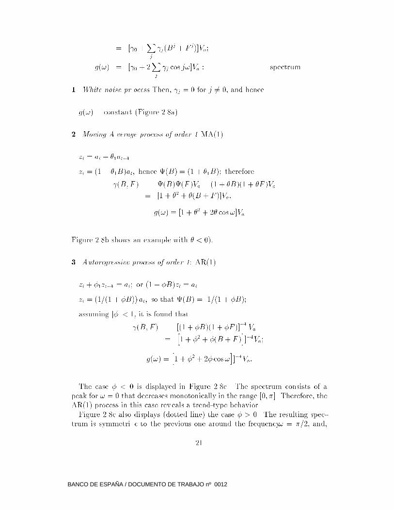
= [ 0 +Xj
j(Bj + F
j)]Va;
g(!) = [ 0 + 2Xj
j cos j!]Va : spectrum.
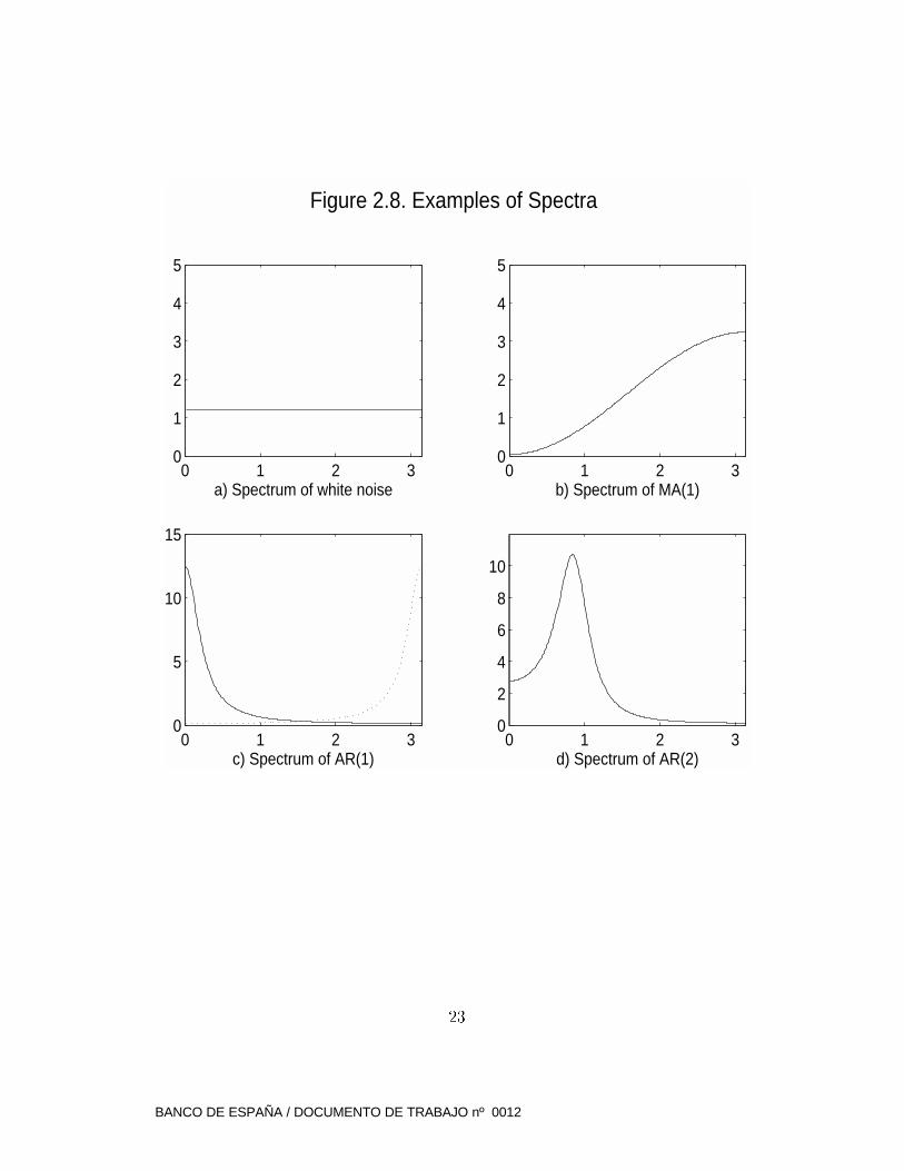
1. White noise pr ocess. Then, j = 0 for j 6= 0, and hence
g(!) = constant (Figure 2.8a).
2. Moving A verage process of order 1: MA(1)
zt = at + �1at�1
zt = (1 + �1B)at; hence (B) = (1 + �1B); therefore
(B;F ) = (B)(F )Va = (1 + �B)(1 + �F )Va =
= [1 + �2 + �(B + F )]Va;
g(!) = [1 + �2 + 2� cos!]Va
Figure 2.8b shows an example with � < 0):
3. Autoregressive process of order 1: AR(1)
zt + �1zt�1 = at; or (1 + �B)zt = at
zt = (1=(1 + �B)) at; so that (B) = 1=(1 + �B);
assuming j�j < 1, it is found that
(B;F ) = [(1 + �B)(1 + �F )]�1Va =
=h1 + �
2 + �(B + F )i]�1Va;
g(!) =h1 + �
2 + 2� cos!i]�1Va:
The case � < 0 is displayed in Figure 2.8c. The spectrum consists of a
peak for ! = 0 that decreases monotonically in the range [0; �]. Therefore, the
AR(1) process in this case reveals a trend-type behavior.
Figure 2.8c also displays (dotted line) the case � > 0. The resulting spec-
trum is symmetri c to the previous one around the frequency! = �=2, and,
21
BANCO DE ESPAÑA / DOCUMENTO DE TRABAJO nº 0012
consequently, displays a peak for ! = �. The period associated with that peak
is, according to (2.13), always 2. Therefore the AR(1) in this case rev eals a
cyclical behavior with period � = 2. If the data is monthly, this behavior cor-
responds to the six-times-a-y ear seasonal frequency; for a quarterly time series,
to the twice-a-year seasonal frequency; for annual data, it would represent a
two-year cycle e�ect.
4. Autoregressive process of order 2: AR(2)
zt + �1zt�1 + �2zt�2 = at (2.31)
or:
(1 + �1B + �2B2)zt = at (2.32)
Concentrating, as we did earlier, on the homogenous part of (2.31), the c har-
acteristic equation associated with that part is precisely the polynomial in B,
with B = r�1. Thus we can �nd the dominant behavior of zt from the solution
of r2 + �1r + �2 = 0. Two cases can happen:
(a) The two roots are real;
(b) The two roots are complex conjugates.
22
BANCO DE ESPAÑA / DOCUMENTO DE TRABAJO nº 0012
0 1 2 30
1
2
3
4
5
a) Spectrum of white noise0 1 2 3
0
1
2
3
4
5
b) Spectrum of MA(1)
0 1 2 30
5
10
15
c) Spectrum of AR(1)
Figure 2.8. Examples of Spectra
0 1 2 30
2
4
6
8
10
d) Spectrum of AR(2)
23
BANCO DE ESPAÑA / DOCUMENTO DE TRABAJO nº 0012
In case (a), if r1 and r2 are the two roots (we assume jr1j and jr2j are < 1),
the polynomial can be factorized as (1 � r1B)(1 � r2B), and each factor will
produce the e�ect of an AR(1) process. Th us, if both r1 and r2 are > 0, the
spectrum will displa y a peak for! = 0; if one is > 0 and the other < 0, the
spectrum will ha ve peaks for ! = 0 and ! = �; if both roots are < 0, the
spectrum will ha ve a peak for! = �.
In case (b), the complex conjugate roots will generate a cosine-t ype (cyclical)
behavior. The modulus m and the frequency ! can be obtained from the model
(2.31) through
m =q�2; ! = arccos
�1
2m
!; (2.33)
and the spectrum will displa y a peak for the frequency!, as in Figure 2.8d.
In general, a useful way to look at the structure of an autoregressive process
of order p, AR(p), a speci�cation very popular in econometrics, is to factorize
the full AR polynomial. Real roots will imply spectral peaks of the t ype 2.8c,
while complex conjugate roots will produce peaks of the type 2.8d.
The range of cyclical frequencies
As already men tioned, the periodic and symmetric character of the spectrum
permits us to consider only the range of frequencies [0; �]. When ! = 0, the
period � !1, and the frequency is associated with a trend. When ! = �=2,
the period equals 4 quarters and the frequency is associated with the �rst
seasonal harmonic (the once-a-y ear frequency). For a frequency in the range
[0 + �1; �=2 � �2], with �1; �2 > 0 and �1 < �=2 � �2, the associated period
will be longer than a year, and bounded. Economic cycles should thus have a
spectrum concen trated in this range. Broadly, we shall refer to this range as
the \range of cyclical frequencies".
Frequencies in the range [�=2; �] are associated with periods between 4 and
2 quarters. Therefore, they imply v ery short-term mo vements (with the cy-
cle completed in less than a y ear) and are of no interest for business-cycle
analysis. Given that ! = � is a seasonal frequency (the twice-a-year seasonal
harmonic), the open in terval of frequencies (�=2; �), excluding the two seasonal
frequencies, will be referred to as the \range of intraseasonal frequencies".
The determination of �1 and �2 in order to specify the precise range of cycli-
cal frequencies is fundamen tally subjective, and depends on the purpose of
the analysis. For quarterly data and business-cycle analysis in the context of
short-term economic policy, obviously a cycle of period 100000 years should be
included in the trend, not in the business cycle. The same consideration w ould
apply to a 10000 years cycle. As the period decreases (and �1 becomes bigger),
we eventually approach frequencies that can be of interest for business-cycle
24
BANCO DE ESPAÑA / DOCUMENTO DE TRABAJO nº 0012
analysis. For example, if the longest cycle that should be considered is a 10
year cycle (40 quarters), from (2.13), �1 should be set as :05�.
At the other extreme of the range, very small values of �2 can produce cycles
with, for example, a period of 1.2 y ears, too short to be of cyclical interest. If
the minim um period for a cycle is set as 1.5 y ears, then�2 should be set equal
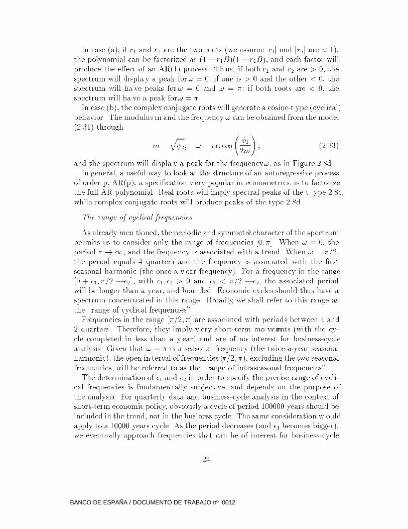
to :167�, and the range of cyclical frequencies would be [:05�; :33�]. Figure 2.9
shows how, from the decision on what is the relevant interval for the periods
in a cyclical componen t, the range of cyclical frequencies is easily determined
(in the �gure, the interval for the period goes from 2 to 12 y ears).
Figure 2.9. Cyclical period and frequency
0 0.5 1 1.5 2 2.5 frequency0
20
40
60
80
100
period
range of cyclical frequencies
Extension to nonstationary unit roots
In the AR(1) model, w e can let� approach the value � = �1. In the limit
we obtain
(1 �B)zt = at; or rzt = at;
the popular random-w alk model. Proceeding as in case 3. abo ve, one obtains
g(!) =1
2(1 � cos!)Va:
For ! = 0, g(!)!1, and hence the integral (2.27) does not converge, which
is in agreemen t with the well-known result that the variance of a random w alk
is unbounded. The nonstationarity induced by the root � = �1 in the AR
25
BANCO DE ESPAÑA / DOCUMENTO DE TRABAJO nº 0012
polynomial (1 + �B), a unit root associated with the zero frequency, induces
a point of in�nite in the spectrum of the process for that frequency. This
result is general: a unit AR root, associated with a particular frequency !0,
will produce an 1 in the spectrum for that particular frequency.
An importan t example is when the polynomialS = 1+B+B2+B3 is present
in the AR polynomial of the series. Giv en that S factorizes into (1+B)(1+B2),
its roots are -1, and �i, associated with the frequencies � and �=2, respectively
(as seen in Section 2.3). The Fourier transform of S, giv en by
S� = 4(1 + cos !)(1 + cos 2!);
displays zeros for ! = � (�rst factor), and ! = �=2 (second factor). Because
S� will appear in the denominator of the spectrum, its zeros will induce poin ts
of 1. Therefore, a model with an AR polynomial including S will ha ve a
spectrum with points of 1 for the frequencies ! = �=2, and ! = �, i.e., the
seasonal frequencies.
It follows that, in the usual case of a seasonal quarterly series, for which a
rr4 or a r2r4 di�erencing has been used as the stationary transformation,
the spectrum of the series w ould present points of1 for the frequencies ! = 0,
! = �=2, and ! = �. Figure 2.10a exhibits what could be the spectrum of a
standard, relatively simple quarterly series.
One �nal point. Given that a spectrumwith poin ts of1 has a nonconvergent
integral, and that no standardization can provide a proper spectral density,
the term spectrum is usually replaced b y Pseudo-spectrum (see, for example,
Hatanaka and Suzuki, 1967, and Harvey, 1989). For our purposes, however,
the points of 1 pose no serious problem, and the pseudo-spectrum can be
used in much the same way as the stationary spectrum (this will become clear
throughout the discussion). In particular, if, for the nonstationary series, we
use the nonconvergent representation (2.18), compute the function (B;F )
through (2.19) and, in the line of Hatanaka and Suzuki, refer to this function
as the \pseudo-AGF", the pseudo-spectrum is the F ourier transform of the
pseudo-AGF. Bearing in mind that, when referring to nonstationary series,
the term \pseudo-spectrum" w ould be more appropriate, in order to a void
excess notation, we shall simply use the term spectrum in all cases.
2.6 Linear �lters and their squared gain
Back to the linear �lter (2.4) of Section 2.1, the �lter can be rewritten as
yt = C(B;F )xt; (2.34)
26
BANCO DE ESPAÑA / DOCUMENTO DE TRABAJO nº 0012
where
C(B;F ) =k1Xj=1
c�jBj + c0 +
k2Xj=1
cjFj:
If k1 = k2 and cj = c�j for all j values, the �lter becomes cen tered and
symmetri c, and we can express it as
C(B;F ) = c0 +kX
j=1
cj(Bj + F
j): (2.35)
Using the same F ourier transform as with expression (2.24), that is, replac-
ing (Bj + Fj) by (2 cos j!), the frequency domain represen tation of the �lter
becomes
C�(!) = c0 + 2
kXj=1
cj cos(|!): (2.36)
If k1 6= k2 or cj 6= c�j , the uncentered or asymmetric �lter does not accept an
expression of the type (2.36). Additional terms in volving imaginary numbers
that do not cancel out will be present. This feature will induce a Phase e�ect in
the output, in the sense that there will be a systematic distortion in the timing
of events between input and output (for example, in the dating of turning
points, of peaks and throughs, etc.). For our purposes, this is a disturbing
feature and hence we shall concentrate attention on centered and symmetric
�lters.
Being C(B,F) symmetric and xt stationary, (2.34) directly yields
AGF (y) = [C(B;F )]2ACF (x);
so that, applying the Fourier transform, w e obtain
gy(!) = [G(!)]2gx(!) (2.37)
where gx(!) and gy(!) are the spectra of the input and output series xt and
yt and we represent by G(!) the Fourier Transform of C(B;F ). The function
G(!) will be denoted the Gain of the �lter. From the relationship (2.37),
the squared gain determines what is the con tribution of the variance of the
input in explaining the variance of the output for each di�erent frequency. If
G(!) = 1, the full variation of x for that frequency is passed to y; if G(!) = 0,
the variation of x for that frequency is fully ignored in the computation of y.
When in terest centers in the componen ts of a series, where the componen ts
are fundamen tally characterized by their frequency properties, the squared
gain function becomes a fundamen tal tool, since it tells us which frequencies
will contribute to the component and which frequencies will not enter it. As an
example, consider a quarterly series with spectrum that of Figure 2.10a. The
peaks for ! = 0; �=2, and � imply that the series con tains a trend componen t
27
BANCO DE ESPAÑA / DOCUMENTO DE TRABAJO nº 0012
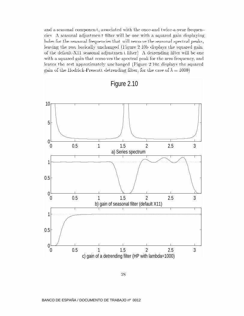
and a seasonal componen t, associated with the once-and twice-a-year frequen-
cies. A seasonal adjustmen t �lter will be one with a squared gain displaying
holes for the seasonal frequencies that will remo ve the seasonal spectral peaks,
leaving the rest basically unchanged (Figure 2.10b displays the squared gain
of the default-X11 seasonal adjustmen t �lter). A detrending �lter will be one
with a squared gain that remo ves the spectral peak for the zero frequency, and
leaves the rest approximately unc hanged (Figure 2.10c displays the squared
gain of the Hodrick-Prescott detrending �lter, for the case of � = 1000).
0 0.5 1 1.5 2 2.5 30
5
10
a) Series spectrum
0 0.5 1 1.5 2 2.5 30
0.5
1
b) gain of seasonal filter (default X11)
Figure 2.10
0 0.5 1 1.5 2 2.5 30
0.5
1
c) gain of a detrending filter (HP with lambda=1000)
28
BANCO DE ESPAÑA / DOCUMENTO DE TRABAJO nº 0012

One �nal importan t clari�cation should be made. W e said that, in order to
avoid phase e�ects, symmetric and cen tered �lters would be considered. Let
one such �lter be
yt = ckxt�k + : : :+ c1xt�1 + c0xt + c1xt+1 + : : :+ ckxt+k: (2.38)
Assume a long series and let T denote the last observ ed period. WhenT � t+k,
the �lter can be applied to obtain yt with no problem. Ho wever, whenT < t+k,
observations at the end of the series, needed to compute yt, are not available
yet, and hence the �lter cannot be applied. As a consequence, the series ytcannot be obtained for recent enough periods, because unknown future ob-
servations of xt are needed. The fact that interest typically centers on recent
periods has lead �lter designers to modify the w eights of the �lters when trun-
cation is needed because a lack of future observations (see, for example, the
analysis in Burridge and W allis, 1984, in the context of the seasonal adjust-
men t �lter X11.) Application of these truncated �lters yields a preliminary
measure of yt, because new observations will imply c hanges in the weights, until
T � t+ k and the �nal (or historical) value of yt can be obtained. One mod-
i�cation that has become popular is to replace needed future values, not yet
observed, by their optimal forecasts, often computed with an ARIMA model
for the series xt. Given that the forecasts are linear functions of present and
past values of xt, the preliminary value of yt obtained with the forecasts will
be a truncated �lter applied to the observed series. Naturally, preliminary
(truncated) �lters will not be centered, nor symmetric . (In particular, the
measurement of yt obtained when the last observed period is t, i.e., when T=t,
the so-called \concurrent" estimator, will be a purely one-sided �lter). Besides
its natural appeal, replacing unknown future values with optimal forecasts has
the convenient features of minimi zing (within the limitations of the structure
of the particular series at hand,) both, the phase e�ect, and the size of the
total revision the preliminary estimator will undergo un til it becomes �nal. To
this importan t issue of preliminary estimation and revisions w e shall return in
the following sections.
29
BANCO DE ESPAÑA / DOCUMENTO DE TRABAJO nº 0012
3 ARIMA models and signal extraction
3.1 ARIMA models
Back to the Wold representation (2.18) of a stationary process, zt = (B)at,
the representation is of no help from the poin t of view of �tting a model
because, in general, the polynomial (B) will contain an in�nite number of
parameters. Therefore w e use a rational approximation of the t ype
(B) _=�(B)
�(B);
where �(B) and �(B) are �nite polynomials in B of order q and p, respectiv ely.
Then we can write
zt =�(B)
�(B)at; or
�(B)zt = �(B)at: (3.1)
The model
(1 + �1B + : : :+ �pBp)zt = (1 + �1B + : : :+ �qB
q)at (3.2)
is the Autoregressive Moving-Average process of orders p and q; in brief, the
ARMA(p,q) model. F or further reference, the Inverse Model of (3.1) is the one
that results from in terchanging the AR and MA polynomials. Thus
�(B)yt = �(B)bt;
with bt white noise, is an inverse model of (3.1). Equation (3.2) can be seen as a
non-homogeneous di�erence equation with forcing function �(B)at, an MA(q)
process. Therefore, if both sides of (3.2) are m ultiplied byzt�k, with k > q,
and expectations are taken, the right hand side of the equation vanishes, and
the left hand side becomes:
k + �1 k�1 + : : :+ �p k�p = 0; (3.3)
or
�(B) k = 0; (3.4)
where B operates on the subindex k. The Eventual Autocorrelation Function
(that is, k as a function of k, for k > q) is the solution of the homogeneous
di�erence equation (3.3), with characteristic equation
rp + �1r
p�1 + : : :+ �p = 0: (3.5)
30
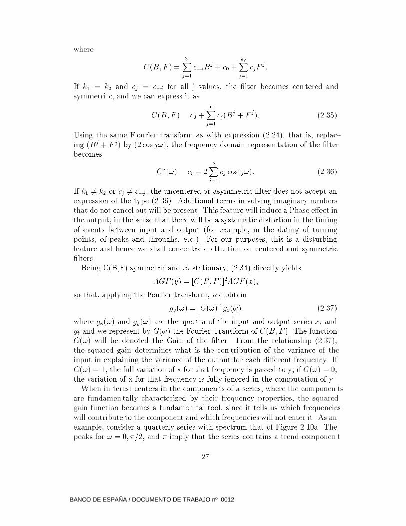
BANCO DE ESPAÑA / DOCUMENTO DE TRABAJO nº 0012
If r1; : : : ; rp are the roots of (3.5) the solution of (3.3) can be written as
k =pX
i=1
rki ;
and will converge to zero as k !1 when jrij < 1; i = 1; : : : ; p. Comparison of
(3.5) with (3.3) shows that r1; : : : ; rp are the inverses of the roots B1; : : : ; Bp
of the polynomial
�(B) = 0
that is, ri = B�1i . Convergence of k implies, th us, that the roots (in B) of the
polynomial �(B) are all larger than 1 in modulus. This condition can also be
stated as follows: the roots of the polynomial �(B) have to lie outside the unit
circle (of Figure 2.1a). When this happen, w e shall say that the polynomial
�(B) is stable. From the identity
�(B)�1 =1
(1� r1B) : : : (1 � rpB);
it is seen that stability of �(B) implies, in turn, con vergence of its inverse
�(B)�1.
From (2.19), considering that (B) = �(B)=�(B), the AGF of zt is given by
(B;F ) =�(B)
�(B)
�(F )
�(F )Va: (3.6)
and it is straightforward to see that stability of �(B) will imply that the
stationarity conditions of Section 2.4 are satis�ed. The AGF is symmetric
and convergent, and the eventual autocorrelation function is the solution of a
di�erence equation, and hence, in general, a mixture of damped polynomials in
time and periodic functions. The Fourier transform of (3.6) yields the spectrum
of zt, equal to
gz(!) = Va�(e�i!)�(ei!)
�(e�i!)�(ei!); (3.7)
and the integral of gz(!) over 0 � ! � 2� is equal to 2�V ar(zt).
A useful result is the following. If two stationary stochastic processes are
related through
yt = C(B)xt;
then the AGF of yt, y(B;F ), is equal to
y(B;F ) = C(B)C(F ) x(B;F );
where x(B;F ) is the AGF of xt. Finally, a function that will prove helpful
is the Crosscovariance Generating Function (CGF) between two series,xt and
31
BANCO DE ESPAÑA / DOCUMENTO DE TRABAJO nº 0012
yt, with W old representation
xt = �(B)at
yt = �(B)at:
Letting j = E(xtyt�j) denote the lag-j crosscovariance between xt and yt,
j = 0;�1;�2; : : : ; the CGF is given by
CGF (B;F ) =1X�1
jBj = �(B)�(F )�2a:
If, in equation (3.2), the subindex t is replaced by t+k (k a positive integer),
and expectations are taken at time t, the forecast of zt+k made at time t,
namely zt+kjt, is obtained. Viewed as a function of k (the horizon) and for a
�xed origin t, zt+kjt is denoted the Forecast Function. (It will be discussed in
more detail in subsection 3.2.3). Giv en thatEtat+k = 0 for k > 0, it is found
that, for k > q, the forecast function satis�es the equation
zt+kjt + �1zt+k�1jt + : : :+ �pzt+k�pjt = 0;
where zt+jjt = zt+j when j � 0. Therefore, the Eventual Forecast Function is
the solution of
�(B)zt+kjt = 0; (3.8)
with B operating on k. Comparing (3.4) and (3.8), the link bet ween autocor-
relation for lag k (and longer) and k-period-ahead forecast becomes apparen t,
the forecast being simply an extrapolation of correlation: what w e can fore-
cast is the correlation we have detected. For a zero-mean stationary process
the forecast function will converge to zero, following, in general, a mixture of
damped exponen tials and cosine functions.
In summary , stationarity of an ARMA model, which requires the roots (in
B) of the autoregressive polynomial �(B) to be larger than 1 in modulus,
implies the following model properties: a) its A GF converges; b) its forecast
function converges; and c) the polynomial �(B)�1 converges, so that zt accepts
the convergent (in�nite) MA represen tation
zt = �(B)�1�(B)at = (B)at; (3.9)
which is precisely the W old representation. To see some examples, for the
AR(1) model
zt + �zt�1 = at;
the root of 1 + �B = 0 is B1 = �1=�. Thus stationarity of zt implies that
jB1j = j1
�j > 1;
32
BANCO DE ESPAÑA / DOCUMENTO DE TRABAJO nº 0012
or j�j < 1.
For the AR(2) model
zt + �1zt�1 + �2zt�2 = at;
stationarity implies that the two roots,B1 and B2 be larger than one in mod-
ulus. This requires the coe�cien ts�1 and �2 to lie inside the triangular region
of Figure 3.1. The parabola inside the triangle separates the region associ-
ated with complex roots from the one with real roots (Bo x and Jenkins, 1970,
Section 3.2).
If zt is the di�erenced series, for which stationarity can be assumed, that is
zt = Dxt; D = rd; d = 0; 1; 2; : : : ;
then the original nonstationary series xt follows the Autoregressive Integrated
Mo ving-Average process of orders p,d, and q, or ARIMA(p,d,q) model, given
by
�(B)Dxt = �(B)at; (3.10)
p and q refer to the orders of the AR and MA polynomials, respectively, and
d refers to the number of regular di�erences (i.e., the number of unit roots at
the zero frequency). W e shall often use abbreviated notation, namely
AR(p): autoregressive process of order p;
MA(q): mo ving-average process of order q;
ARI(p,d): autoregressive process of order p applied to the dth di�erence of
the series;
IMA(d,q): mo ving-average process of order q applied to thedth di�erence of
the series.
Further, a series will be denoted I(d) when it requires d regular di�erences
in order to become stationary.
33
BANCO DE ESPAÑA / DOCUMENTO DE TRABAJO nº 0012

34
BANCO DE ESPAÑA / DOCUMENTO DE TRABAJO nº 0012
As in the stationary case, taking conditional expectations at time t in both
sides of equation (3.10) with t replaced by t+k, where k is a positive integer,
it is obtained that
�(B)Dxt+kjt = �(B)at+kjt;
where
xt+jjt = E(xt+j j xt; xt�1; : : :)is the forecast of xt+j obtained at time t when j > 0, and is the observation
xt+j when j � 0; further, at+jjt = E(at+j j xt; xt�1; : : :) is equal to 0 when
j > 0, and is equal to at+j when j � 0. As a consequence, the eventual
forecast function (xt+kjt as a function of k, for k > q) will be the solution of
the homogenous di�erence equation
�(B)Dxt+kjt = 0;
with B operating on k. The roots of D all have unit modulus; if D = rd,
then the eventual forecast function will include a deterministic polynomial in
t of the type (a+ btd�1). If D also includes seasonal di�erencing r4, then the
eventual forecast function will also contain the non-convergent deterministic
cosine-type function (2.14), associated with the once and twice-a-year seasonal
frequencies, ! = �=2 and ! = �.
As an example, the forecast function of the model
(1� :7B)rr4xt = (1 + �1B)(1 + �4B4)at;
will consists of �ve starting values xt+jjt; j = 1; : : : ; 5; implied b y the MA part
with q=5, after whic h the function will be the solution of the homogenous
equation associated with the AR part. Factorizing the AR polynomial as
(1 � :7B)(1�B)2(1 +B)(1 +B2);
the roots of the characteristic equation are given by
r1 = :7; r2 = r3 = 1; r4 = �1; r5 = i; r6 = �i:From Section 2.3, the ev entual forecast function can be expressed as
xt+kjt = c(t)1 (:7)k + c
(t)2 + c
(t)3 k + c
(t)4 (�1)k + c
(t)5 cos
��
2k + c
(t)6
�;
where the last two terms re ect the seasonal harmonics (the root r4 = �1 canalso be written as c
(t)4 cos �k). The constants c1; : : : ; c6 are determined from
the starting conditions of the forecast function, and hence will depend on t,
the origin of the forecast. This feature gives the ARIMA model its adaptive
(or \mo ving") properties. Notice that, in the nonstationary case, the forecast
function (with �xed origin t and increasing horizon k) will not converge.
Concerning the MA polynomial �(B), a similar condition of stability will
35
BANCO DE ESPAÑA / DOCUMENTO DE TRABAJO nº 0012
be imposed, namely , the rootsB1; : : : ; Bq of the equation �(B) = 0 have to
be larger than 1 in modulus. This condition is referred to as the In vertibility
condition for the process and, unless otherwise speci�ed, we shall assume that
the model for the observ ed serieszt is invertible. This assumption implies that
�(B)�1 converges, so that the model (3.1) can be in verted and expressed as
at = �(B)�1�(B)zt = �(B)zt; (3.11)
which shows that the series accepts a convergent (in�nite) AR expression, and
hence can be approximated b y a �nite AR. Expression (3.11) also shows that,
when the process is invertible, the innovations can be recovered from the ztseries.
Some frequency domain implications of nonstationarit y and noninvertibility
are worth pointing out. Assume that the MA polynomial �(B) has a unit root
jB1j = 1 -perhaps a complex conjugate pair- associated with the frequency !1.
Then, �(e�i!1) = 0, and the spectrum of zt, given by (3.7), will have a zero
for the frequency !1. Analogously, if jB1j = 1 is a root of the AR polynomial
�(B), with associated frequency !1, then, �(e�i!1) = 0, and g(!1)!1
. It follows that
� a unit MA root causes a zero in the spectrum;
� a unit AR root causes a point of 1 in the spectrum;
� an invertible model will ha ve strictly positive spectrum,g(!) > 0;
� a stationary model has a bounded spectrum, g(!) <1:
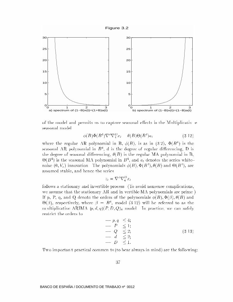
To illustrate the spectral implications of unit roots, Figure 3.2a presen ts the
spectrum of the model
(1 �B)xt = (1 +B)at:
Since the spectrum is proportional to (1+cos!)=(1�cos!), the unit AR root
B = 1 for the zero frequency mak es the vertical axis an asymptote. The unit
MA root B = �1 for ! = � creates a zero for this frequency. The spectrum of
the inverse model
(1 +B)xt = (1 �B)atis displayed in Figure 3.2b. The unit AR root for ! = � implies that the line
! = � is an asymptote, and the unit MA root for ! = 0 implies a spectral zero
at the origin.
For quarterly data with seasonality, the di�erencing D is likely to contain
the seasonal di�erence r4. A popular speci�cation that increases parsimon y
36
BANCO DE ESPAÑA / DOCUMENTO DE TRABAJO nº 0012
0 1 2 30
5
10
15
20
25
30
a) spectrum of (1−B)x(t)=(1+B)a(t)
Figure 3.2
0 1 2 30
5
10
15
20
25
30
b) spectrum of (1−B)x(t)=(1−B)a(t)
of the model and permits us to capture seasonal e�ects is the Multiplicativ e
seasonal model
�(B)�(B4)rdrD4 xt = �(B)�(B4)at (3.12)
where the regular AR polynomial in B, �(B), is as in (3.2), �(B4) is the
seasonal AR polynomial in B4, d is the degree of regular di�erencing, D is
the degree of seasonal di�erencing, �(B) is the regular MA polynomial in B,
�(B4) is the seasonal MA polynomial in B4, and at denotes the series white-
noise (0; Va) innovation. The polynomials �(B);�(B4); �(B) and �(B4), are
assumed stable, and hence the series
zt = rdrD4 xt
follows a stationary and invertible process. (To avoid nonsense complications,
we assume that the stationary AR and in vertible MA polynomials are prime.)
If p, P, q, and Q denote the orders of the polynomials �(B);�(�); �(B) and
�(�), respectively, where � = B4, model (3.12) will be referred to as the
multiplicative ARIMA (p; d; q)(P;D;Q)4 model. In practice, we can safely
restrict the orders to
� p; q � 4;
� P � 1;
� Q � 2;
� d � 2;
� D � 1:
(3.13)
Two importan t practical commen ts (to bear always in mind) are the following:
37
BANCO DE ESPAÑA / DOCUMENTO DE TRABAJO nº 0012
1. Parsimon y (i.e., few parameters) should be a crucial propert y of ARIMA
models used in practice.
2. ARIMAmodels are a useful tool for relatively short-term analysis. Their
exibility and adaptive behavior contribute to their good short-term fore-
casting. Long-term extrapolation of this exibility may imply, however,
unstable long-term inference (see Mara vall, 1999). As a general rule,
short-term analysis fa vors di�erencing, while long-term one fa vors more
deterministic trends, that imply less di�erences.
3.2 Modelling strategy, diagnostics and inference
The so-called Box-Jenkins approach to building ARIMA models consists of the
following iterative scheme that con tains 4 stages:
3.2.1 Identi�cation
Two features of the series have to be addressed,
� the degree of regular and seasonal di�erencing;
� the orders of the stationary AR and invertible MA polynomials.
Di�erencing of the series can emplo y some of the unit root tests a vailable for
possibly seasonal data (see, for example, Hylleberg et al, 1990). Devised to test
deterministic seasonals v ersus seasonal di�erencing, these test are of little use
for our purpose. In our experience, stochastic modelling remo ves in practice the
need for the dilemm a: deterministic speci�cation v ersus di�erencing. Consider,
for example, the two models:
(a) xt = � + at,
(b) rxt = (1� :99B)at:
For a quarterly series, and realistic series length, it is impossible that the
sample information can distinguish bet ween the two speci�cations. Conse-
quently, the choice is arbitrary. Besides the variance of at, Model (a) con tains
one parameter that needs to be estimated, while Model (b) con tains none (al-
though, in this case the �rst observation is lost by di�erencing). Model (a)
o�ers, thus, no estimation advantage. If short-term forecasting is the main
objective, however, Model (b) will display some advantage because it allows
for more exibilit y, given that it could be rewritten as xt = �(t) + at, where
�(t) is a very slowly adapting mean.
A similar consideration applies to seasonal v ariations. The model
38
BANCO DE ESPAÑA / DOCUMENTO DE TRABAJO nº 0012
(c) xt = �+P3
j=1 �jdjt + at;
where djt denotes a quarterly seasonal dummy variable, is in practice indis-
tinguishable from the direct speci�cation
(d) r4xt = (1 � :95B4)at:
The deterministic speci�cation has no w 4 parameters; the stoc hastic one has
none, but 4 starting values are lost at the beginning.. The latter can also be
expressed as
xt = �(t) +
3Xj=1
�(t)j djt + at;
where �(t); �(t) denote slowly adapting coe�cien ts. Within our short-term
perspective, there is no reason thus to main tain the deterministic-stoc hastic di-
chotomy, and deterministic features can be seen as extremely stable stoc hastic
ones.
Besides the lack of power of unit roots tests to distinguish between models
(a) and (b), or (c) and (d), the process of building ARIMA models typically
implies estimation of man y speci�cations (if combined with outlier detection
and correction, the number may be indeed very large) and the true size of the
tests is therefore unknown. In practice, a more e�cien t and reliable proce-
dure for determining AR unit roots is to use estimation results based on the
superconsistency of parameter estimates associated with unit roots, ha ving de-
termined \a priori" how close to one a root has to be in order to be considered
a unit root (see Tiao and Tsay, 1983, 1989, and G�omez and Mara vall, 2000a).
Once the proper di�erencing has been established, it remains to determine
the orders of the stationary AR and invertibleMA polynomials. Here, the basic
criterion used to be to try to match the SACF of zt with the theoretical ACF
of a particular ARMA process. In recent years, the e�ciency and reliability of
automatic iden ti�cation procedures, based mostly on information criteria, has
strongly decreased the importance of the \ten tative identi�cation" stage (see
Fischer and Planas, 1999, and G�omez and Mara vall, 2000a).
3.2.2 Estimation and diagnostics
When q 6= 0, the ARIMA residuals are highly nonlinear functions of the model
parameters, and hence n umerical maximiz ation of the likelihood function, or
of some function of the residual sum of squares, can be computationally non-
trivial. Within the restrictions in the size of the model giv en by (3.13), how-
ever, maximi zation is typically well behaved. A standard estimation proce-
dure would cast the model in a state-space format, and use the Kalman �lter
39
BANCO DE ESPAÑA / DOCUMENTO DE TRABAJO nº 0012
to compute the lik elihood through the Prediction Error Decomposition. The
likelihood is then maximized with some nonlinear procedure. Usually, the
Va parameter, as w ell as a possible constant mean, are concen trated out of
the likelihood. When the series is nonstationary , several solutions have been
proposed to overcome the problem of de�ning a proper lik elihood. Relevant
references are Bell and Hillme r (1991), Brockwell and Davis (1987), De Jong
(1991), G�omez and Mara vall (1994), Kohn and Ansley (1986), and Morf, Sidh u
and Kailath (1974). Several of these references deal, in fact, with more general
models than the straigh tforward ARIMA one.
Man y diagnostics are available for ARIMA models. A crucial one, of course,
is the out-of-sample forecast performance. Some test for in-sample model
stability are also of interest. Then, there is a large set of test based on the
model residuals, assumed to be niid. This implies testing for Normality, for
autocorrelation, for homoscedasticit y, etc. Besides the ones proposed by Box
and Jenkins (1970), additional references can be Newbold (1983), Gourieroux
and Monfort (1990), Harv ey (1989), and Hendry (1995).
3.2.3 Inference
If the diagnostics are failed, in the light of the results obtained, the model
speci�cation should be changed. When the model passes all diagnostics, w e
ma y then proceed to inference. W e shall look in particular at an application
in forecasting, unquestionably the main use of ARIMA models.
Let (3.10) denote, in compact notation, the ARIMA model identi�ed for the
series xt, and, as in Section 3.1, denote by xt+jjt the forecast of xt+j made at
period t (in Box-Jenkins notation, xt+jjt = xt(j).) Under our assumptions, the
optimal forecast of xt+j, in a Minim um Mean Square Error (MMSE) sense,
is the expectation of xt+k conditional on the observed time series x1; : : : ; xt(equal also, to the projection of xt+k onto the observed time series); that is,
xt+jjt = E(xt+k j x1; : : : ; xt):This conditional expectation can be obtained with the Kalman �lter, or with
the Box-Jenkins procedure (for large enough t). Recall that, for known pa-
rameters,
at = xt � xtjt�1;
that is, the innovations of the process are the sequence of one-period-ahead
forecast errors.
The forecast function at time t is xt+kjt as a function of k (k a positive
integer). In Section 3.1 we saw that for an ARIMA (p,d,q) model, the forecast
function consists of q starting conditions, after which it is given by the solution
40
BANCO DE ESPAÑA / DOCUMENTO DE TRABAJO nº 0012
of the homogenous AR di�erence equation
��(B)xt+kjt = 0; (3.14)
where B operates on k, and ��(B) denotes the full AR convolution ��(B) =
�(B)D, and includes thus the unit roots.
A useful way to look at forecasts is directly based on the pure MA represen-
tation (B), even in the nonstationary case of a nonconvergent (B). Assume
the model parameter are kno wn and write
xt+k = at+k + 1at+k�1 + : : :+ k�1at+1 + kat + k+1at�1 + : : : : (3.15)
Given that, for k > 0, Etat+k = 0 and Etat�k = at�k, taking conditional
expectations in (3.15) yields
xt+kjt = Etxt+k =1Xj=0
k+jat�j; (3.16)
so that the forecast is a linear combination of past and present innovations.
Substracting (3.16) from (3.15), the k-periods-ahead forecast error is given by
the model
et+kjt = xt+k � xt+kjt
= at+k + 1at+k�1 + : : :+ k�1at+1; (3.17)
an MA(k-1) process of \future" inno vations. From expression (3.17), the join t,
marginal, and conditional distributions of forecast errors can be easily deriv ed,
and in particular the standard error of the k-period ahead forecast, equal to
SE(k) = (1 + 21 + : : :+
2k�1)
1=2�a: (3.18)
Unless the series is relatively short, this standard error, estimated by using
ML estimators of the parameters, will pro vide a good approximation. Figure
3.3 displays the last 3 years of observations and the next 2 years of ARIMA
forecasts for a quarterly series. The forecast function is dominated b y a linear
trend plus seasonal oscillations; the width of the con�dence interval increases
with the horizon.
41
BANCO DE ESPAÑA / DOCUMENTO DE TRABAJO nº 0012
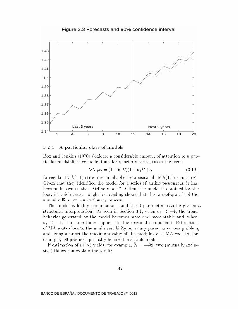
Figure 3.3 Forecasts and 90% confidence interval
2 4 6 8 10 12 14 16 18 201.34
1.35
1.36
1.37
1.38
1.39
1.4
1.41
1.42
1.43
Last 3 years Next 2 years
3.2.4 A particular class of models
Box and Jenkins (1970) dedicate a considerable amoun t of attention to a par-
ticular multiplicative model that, for quarterly series, tak es the form
rr4xt = (1 + �1B)(1 + �4B4)at (3.19)
(a regular IMA(1,1) structure m ultiplied by a seasonal IMA(1,1) structure).
Given that they identi�ed the model for a series of airline passengers, it has
become known as the \Airline model". Often, the model is obtained for the
logs, in which case a rough �rst reading shows that the rate-of-growth of the
annual di�erence is a stationary process.
The model is highly parsimonious, and the 3 parameters can be giv en a
structural interpretation. As seen in Section 3.1, when �1 ! �1, the trend
behavior generated by the model becomes more and more stable and, when
�4 ! �1, the same thing happens to the seasonal componen t. Estimation
of MA roots close to the nonin vertibility boundary poses no serious problem,
and �xing a priori the maximum value of the modulus of a MA root to, for
example, .99 produces perfectly beha ved invertible models.
If estimation of (3.19) yields, for example, �4 = �:99, two (mutually exclu-sive) things can explain the result:
42
BANCO DE ESPAÑA / DOCUMENTO DE TRABAJO nº 0012
1) seasonality is practically deterministic;
2) there is no seasonality, and the model is o verdi�erenced.
Determining whic h of the two is the correct explanation is rather simple b y
testing for the signi�cance of seasonal dummy variables. When the model has
no seasonality, the seasonal �lter r4zt = (1� :99B4)bt would have hardly any
e�ect on the input series. A similar reasoning holds for �1 and the possible
presence of a deterministic trend. Further, a purely white-noise series �ltered
with model (3.19) with �1 = �4 = �:99 would, very approximately, reproduce
the series. Thus the Airline model also encompasses simpler structures with no
trend or no seasonality. Adding the empirical fact that it pro vides reasonably
good �ts to man y actual macroeconomic series (see, for example, Fisc her and
Planas, 1999, or Mara vall, 2000), it is an excellent model for illustration, for
benchmark comparison, and for pre-testing.
3.3 Preadjustment
We have introduced the ARIMA model as a practical way of dealing with
mo ving features of series. Still, before considering a series appropriate for
ARIMA modelling, several prior corrections or adjustments may be needed.
W e shall classify them in to 3 groups.
1. OUTLIERS
The series ma y be subject to abrupt changes, that cannot be explained
by the underlying normalit y of the ARIMA model. Three main types of
outlier e�ects are often distinguished: a) additive outlier, which a�ects
an isolated observation, b) level shift, which implies a step c hange in the
mean lev el of the series, and c) transitory change, similar to an additiv e
outlier whose e�ect damps out o ver a few periods. Chen and Liu (1993)
suggested an approach to automatic outlier detection and correction that
has lead to reliable and e�cien t procedures (see G�omez and Mara vall,
2000a).
2. CALEND AR EFFECT
By this term w e refer to the e�ect of calendar dates, such as the number
of working days in a period, the location of Easter e�ect, or holidays.
These e�ects are typically incorporated into the model through regression
variables (see, for example, Hillme r, Bell and Tiao, 1983, and Harv ey,
1989).
43
BANCO DE ESPAÑA / DOCUMENTO DE TRABAJO nº 0012
3. INTERVENTION V ARIABLES
Often special, unusual events a�ect the evolution of the series and can-
not be accounted for by the ARIMA model. There is thus a need to
\intervene" the series in order to correct for the e�ect of special events.
Examples can be strik es, devaluations, change of the base index or of the
way a series is constructed, natural disasters, political events, importan t
tax changes, or new regulations, to men tion a few. These special e�ects
are entered in the model as regression variables (often called, following
Box and Tiao, 1975, intervention variables).
The full model for the observ ed series can thus be written as
yt = w0
t� + C0
t� +kX
j=1
�j�j(B)It(tj) + xt (3.20)
where � = (�1; : : : ; �n)0, is a vector of regression coe�cients,w0
t = (w1t; : : : ; wnt)
denotes n regression or intervention variables, C 0
t denotes the matrix with
columns the calendar e�ect variables (trading day, Easter e�ect, Leap year ef-
fect, holidays), and � the vector of associated coe�cien ts,It(tj) is an indicator
variable for the possible presence of an outlier at period tj, �j(B) captures
the transmission of the j-th outlier e�ect (for additiv e outliers,�j(B) = 1, for
level shifts, �j(B) = 1=r, for transitory changes, �j(B) = 1=(1 � �B), with
0 < � < 1;) and �j denotes the coe�cien t of the outlier in the multiple regres-
sion model with k outliers. Finally ,xt follows the general (possibly m ultiplica-
tive) ARIMA model (3.12). As mentioned earlier, there are several procedures
for estimation of models of this t ype, and easily available programs that en-
force the procedures (examples are the programs REGARIMA, see Findley
et al, 1998, and TRAMO, see G� omez and Mara vall, 1996).Noticing that
intervention variables, outliers, and calendar e�ects are regression variables,
the full model can be expressed as a regression-ARIMA model. Estimation
typically proceeds by iterating as follows: conditional on the regression pa-
rameters (�; �; �), exact maximum likelihood estimation of the ARIMA model
is performed; then, conditional on the ARIMA model, GLS estimators of the
regression parameters are obtained (both steps can be done with the Kalman
�lter).
Bearing in mind that preadjustment should be a \must" in applied time
series work, for the rest of this book, we shall assume that the series do not
require preadjustment, or have already been subject to one. The series can be
directly seen, then, as the outcome of an ARIMA process.
Figures 3.4 and 3.5 illustrate preadjustmen t in quarterly (simulated) series.
The observed original series is displayed in Figure 3.4a. After remo val (through
regression) of the outliers automatically iden ti�ed in the series (2 additive
44
BANCO DE ESPAÑA / DOCUMENTO DE TRABAJO nº 0012
outliers, 1 level shift, and 1 transitory change) whose e�ect is displayed in
Figure 3.5a, of the trading-day e�ect (captured, in this case, with a variable
that counts the number of working days) shown in Figure 3.5b, of the Easter
e�ect, exhibited in Figure 3.5c, and of an intervention variable associated with
the introduction of a regulation that a�ects the seasonal e�ect for the last two
quarters of each year, the remaining series is displa yed in Figure 3.4b. This
is the preadjusted series, also referred to as the \linearized series", given that
it can be assumed the output of a linear stoc hastic process (modelled in the
ARIMA format).
In the �nal decomposition of the observ ed series, that we shall be discussing
in the following sections, the di�erent regresion e�ects (outliers, calendar ef-
fects, and intervention variables) can be associated with di�erent componen ts.
Thus, typically, calendar e�ects will be associated with the seasonal compo-
nent, additive and transitory outliers will be assigned to the irregular com-
ponent, and level shifts to the trend-cycle componen t. Care should be taken,
however, when a separate business-cycle componen t is being estimated, be-
cause it ma y require a di�erent allocation of the deterministic e�ects. For
example, when ann ual data is being used, a transitory change that takes 5
or 6 periods to become negligeable should probably be included in the cycle,
not in the irregular. Likewise, the correction produced by two level shifts of
opposite sign and similar magnitude possibly should be assigned to the cycle,
not to the long-term trend.
45
BANCO DE ESPAÑA / DOCUMENTO DE TRABAJO nº 0012
0 10 20 30 40 50 60 70 800.11
0.12
0.13
0.14
0.15
a) observed series
Figure 3.4. Preadjustment
0 10 20 30 40 50 60 70 800.11
0.12
0.13
0.14
0.15
b) preadjusted (linearized) series
46
BANCO DE ESPAÑA / DOCUMENTO DE TRABAJO nº 0012
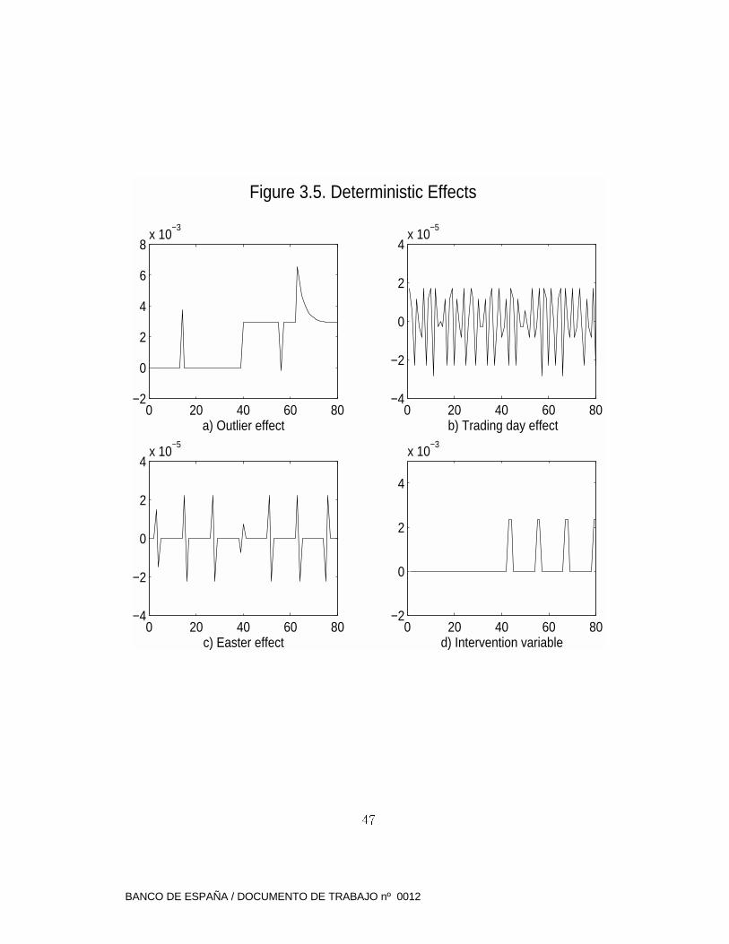
0 20 40 60 80−2
0
2
4
6
8x 10
−3
a) Outlier effect0 20 40 60 80
−4
−2
0
2
4x 10
−5
b) Trading day effect
0 20 40 60 80−4
−2
0
2
4x 10
−5
c) Easter effect
Figure 3.5. Deterministic Effects
0 20 40 60 80−2
0
2
4
x 10−3
d) Intervention variable
47
BANCO DE ESPAÑA / DOCUMENTO DE TRABAJO nº 0012
3.4 Unobserved components and signal extraction
Assume w e are interested in some unobserv ed componen t buried in the ob-
served series. Examples can be the seasonally adjusted (SA) series, some un-
derlying short-term trend, or perhaps some cycle. W e refer to the componen t
of interest as the Signal, and assume it can be extracted from xt in an additive
manner, as in
xt = st + nt; (3.21)
where nt denoted the non-signal componen t of the series. (If the signal is the
SA series, nt would be the seasonal componen t; if the signal is the short-term
trend, an additional noise or transitory component may also be included in nt).
The decomposition can also be m ultiplicative, as inxt = stnt. Taking logs,
however, the additive structure is recovered. For the rest of the discussion we
shall consider the additive decomposition. (A more complete presen tation can
be found in Planas, 1997).
W e further assume that both componen ts are linear stochastic processes, say
�s(B)st = �s(B)ast (3.22)
�n(B)nt = �n(B)ant: (3.23)
The AR polynomials �s(B) and �n(B) also include possible unit roots; in
fact, in the vast majorit y of applications, at least one of the componen ts will
be nonstationary. This is because the very concept of a trend or a seasonal
componen t imply a mean that c hanges with time, and hence a nonstationary
behavior that can be remo ved by di�erencing.
Concerning expressions (3.22) and (3.23), the following assumptions will be
made:
(A.1) The variables ast and ant are mutually independent white-noise pro-
cesses, with zero mean, and v ariancesVs and Vn, respectively.
(A.2) The polynomials �s(B) and �n(B) are prime.
(A.3) The polynomials �s(B) and �n(B) share no unit root in common.
The �rst assumption is based on the belief that what causes, for example,
seasonality (weather, time of y ear) is not much related to what may drive
a long-term trend (tec hnology, investmen t), and similarly for other compo-
nents. Given that di�erent componen ts are associated with di�erent spectral
peaks, assumption A.2 seems perfectly sensible. Assumption A.3 is not strictly
needed, but in practice it is hardly restrictive and simpli�es considerably no-
tation. The assumption states a su�cien t condition for invertibility of thextseries.
48
BANCO DE ESPAÑA / DOCUMENTO DE TRABAJO nº 0012
Because aggregation of ARIMA models also yields an ARIMA model, the
series xt will follow an ARIMA model, which we write as
�(B)xt = �(B)at; (3.24)
where at is a white noise variable, �(B) is invertible, and �(B) is given by
�(B) = �s(B)�n(B): (3.25)
The following identity is implied b y (3.22)-(3.24):
�(B)at = �n(B)�s(B)ast + �s(B)�n(B)ant;
which shows the relatively complicated relationship between the series innova-
tions and the innovations in the componen ts (see Mara vall, 1995)
Having observed a time series XT = [x1; : : : ; xT ] our aim is: 1) to obtain
Minim um Mean Square Error (MMSE) estimators of ^st (and nt), as well as
forecasts; 2) to obtain the full distribution of these estimators, from whic h
diagnostics can be derived; 3) to obtain standard errors for the estimators
and forecasts; and 4) to analyze some importan t features, such as revisions in
preliminary estimators, both in terms of size and speed of con vergence to the
historical estimators.
1. Known models
For the stationary case, the full distribution of (st;XT ) is known. Under
some additional assumptions (see, for example, Bell and Hillmer, 1991, and
G�omez and Mara vall, 1993) an appropriate conditional distribution can also
be derived for the nonstationary case. The joint distribution is multivariate
normal, so that the conditional expectation of the unobserved st, given XT , is
a linear combination of the elements in XT . This conditional expectation also
provides the MMSE estimator, st, which can thus be expressed as the linear
�lter
st = E(st j x1; : : : ; xT ) = �1x1 + �2x2 + : : :+ �TxT :
The above conditional expectation can be computed with the Kalman �lter (see
Harvey, 1989) or with the Wiener-Kolmogorov (WK) �lter (see Bo x, Hillme r
and Tiao, 1978). The equivalence of both �lters, also when the series is nonsta-
tionary, is shown in G�omez (1999). Both �lters are e�cien t; while the Kalman
�lter has a more exible format to expand the models, the WK �lter is more
useful for analysis and interpretation. It will be the one used in the discussion.
W e start by considering the case of an in�nite realization (x�1; : : : x1). (In
practice, this means that w e start with historical estimation for the cen tral
years of a long-enough series.) As shown in Whittle (1963), the WK �lter that
yields the MMSE of st when model (3.24) is stationary is giv en by the ratio of
49
BANCO DE ESPAÑA / DOCUMENTO DE TRABAJO nº 0012
the AGF of st and xt, namely
st =
"AGF (st)
AGF (xt)
#xt =
266664Vs�s(B)�s(F )
�s(B)�s(F )
Va�(B)�(F )
�(B)�(F )
377775xt: (3.26)
Notice that an importan t feature of the WK �lter (enforced in this w ay) is
that it only requires the speci�cation of the model for the signal, once the
model for the observ ed series has been identi�ed. Contrary to other model-
based approaches enforced with the Kalman �lter, suc h as the Structural Time
Series Model (STSM) approach of Harvey (1989), with the WK �lter there is
no need to specify the componen ts that aggregate into the non-signal nt. In
view of (3.25), the �lter simpli�es in to
st =
"ks�s(B)�n(B)
�(B)
�s(F )�n(F )
�(F )
#xt: (3.27)
where ks = Vs=Va. Direct inspection of (3.27) shows that the �lter is the AGF
of the stationary model
�(B)zt = �s(B)�n(B)bt; (3.28)
where bt is white noise with variance (Vs=Va). The �lter is thus convergent in
B and F, centered at t, and symmetric .
In order to analyze the properties of the estimated signal, w e shall be in-
terested in its spectrum. If gs(!); gn(!) and g(!) denote the spectrum of the
signal, the non-signal componen t, and the observed series, respectively, orthog-
onality of st and nt imply
g(!) = gs(!) + gn(!);
where the two componen ts spectra are nonnegative, andg(!) is strictly positive
(due to the invertibility condition on the observed series).
The gain of the WK �lter, given by the expression in brackets in (3.26), is
the Fourier transform of the ratio of t wo AGFs, so that
G(!) = gs(!)=g(!):
Thus, according to (3.26), the spectrum of the MMSE estimator st, denoted
gs(!) is given by
gs(!) =
"gs(!)
g(!)
#2g(!) =
=
"gs(!)
g(!)
#gs(!) =
50
BANCO DE ESPAÑA / DOCUMENTO DE TRABAJO nº 0012
= G(!)gs(!): (3.29)
Given that G(!) � 1, it follows that
gs(!) � gs(!);
and hence the MMSE estimator will underestimate the variance of the theo-
retical componen t.
The �lter is well de�ned everywhere when the �-polynomials con tain unit
roots, and, in fact, extends, in a straightforward manner, to the nonstation-
ary case (see Bell, 1984, and Mara vall, 1988). As for the distribution of the
estimator st, for the general nonstationary case, assume the polynomial �s(B)
can be factorized as
�s(B) = 's(B)Ds;
whereDs contains all unit roots, and 's(B) is a stable polynomial. Multiplying
(3.27) by Ds, and replacing Dsxt by
[�(B)='s(B)�n(B)]at;
it is obtained that
Dsst =
"ks�s(B)
's(B)
�s(F )�n(F )
�(F )
#at; (3.30)
which provides the model that generates the stationary transformation of the
estimator st. It is seen that MMSE estimation preserves the di�erencing of
the theoretical componen t, but has an e�ect on the stationary structure of
the model. The part in B of the model generating the estimator is iden tical
to that of the componen t; the model for the estimator, ho wever, contains a
part in F (that gradually converges towards zero), re ecting the contribution
of innovations posterior to t to the historical estimator for period t. Theo-
retical component, given by (3.22), and MMSE estimator will have the same
stationary transformation, but the A GF and spectra will di�er. Further, it is
straightforward to see that the AGF of the historical estimation error,
et = st � st;
is equal to the AGF of the stationary ARMA model
�(B)zt = �s(B)�n(B)bt; (3.31)
where bt is white noise with variance (VsVn)=Va (see Pierce,1979). Stationarity
of (3.31) implies that componen t and estimator are coin tegrated.
As was men tioned in Section 2.6, for a �nite realization of thext process,
it will happen that, for periods close enough to both ends of the series, it will
not be possible to apply the complete two-sided �lter. Denote by�(B;F ) the
51
BANCO DE ESPAÑA / DOCUMENTO DE TRABAJO nº 0012
�lter in brackets in expression (3.27), namely
�(B;F ) = ks�s(B)�n(B)
�(B)
�s(F )�n(F )
�(F ); (3.32)
and assume it can be safely truncated after L periods, so that w e can write
the historical estimator as
st = �0xt +LXj=1
�j(xt�j + xt+j): (3.33)
Let the time series a vailable be (x1; : : : ; xT ) and, to avoid problems with �rst
observations, let T > L. Assume w e wish to estimatest for t � T and
(T � t) > L, that is for relatively recent periods. According to (3.33), we need
L � (T � t) observations at the end of the �lter that are not available yet,
namely, xT+1; xT+2; : : : ; xT+L�(T�t) . Replacing these future values with the
ARIMA forecasts computed at time T, we obtain the preliminary estimator.
Rewriting (3.33) as
st = �Lxt�L + : : :+ �0xt + : : :+ �(T�t)xT +
+ �(T�t+1)xT+1 + �(T�t+2)xT+2 +
+ : : :+ �Lxt+L; (3.34)
and taking conditional expectations at time T, the preliminary estimator of
the signal for time t, when observ ations end at time T, denoted stjT , is given
by
stjT = �Lxt�L + : : :+ �0xt + : : :+ �(T�t)xT +
+ �(T�t+1)xT+1jT + �(T�t+2)xT+2jT +
+ : : :+ �Lxt+LjT (3.35)
where xt1jt2 denotes the forecasts of xt1 obtained at period t2. Thus, in compact
form, the preliminary estimator can be expressed as
stjT = �(B;F )xetjT (3.36)
where �(B;F ) is the WK-�lter, and xetjT is the "extended" series, such that
xetjT = xt for t � T
xetjT = xtjT for t > T:
The Revision the preliminary estimator will undergo un til it becomes the his-
torical one is the di�erence (st � stjT ) or, substracting (3.35) from (3.34),
rtjT =t+L�TXj=1
�T�t+j eT+jjT ; (3.37)
that is, the revision is a linear combination of the forecast errors. Large re-
52
BANCO DE ESPAÑA / DOCUMENTO DE TRABAJO nº 0012
visions are unquestionably an undesirable feature of a preliminary estimator,
and expression (3.37) shows the close relationship between forecast error and
revision: the better we can forecast the observed series, the smaller the revision
in the preliminary estimator of the signal will be.
Direct application of (3.35), when t is close to the end of the series, ma y re-
quire for models close to nonin vertibility (for which �(B)�1 converges slowly)
a very large number of forecasts (perhaps more than 100) in order to com-
plete the �lter. The Burman-Wilson algorithm (Burman, 1980), permits us
to capture, in a very e�cient way, the e�ect of the in�nite forecast function
with just a small number of forecasts; for the vast majorit y of quarterly series,
10 forecasts are indeed enough. A similar procedure can be applied to the
�rst periods of the sample to impro ve starting values for the signal estimator:
one can extend the series at the beginning with backcasts (see Box and Jenk-
ins, 1970), and apply the WK �lter to the extended series, using a symmetric
Burman-Wilson algorithm.
By com bining (3.24) with (3.27), an expression is obtained that relates the
�nal estimator st to the innovations at in the observed series, to be represented
by
st = �s(B;F )at; (3.38)
where �s(B;F ) can be obtained from the identity
�s(B)�(F )�s(B;F ) = ks�s(B)�s(F )�n(F ); (3.39)
and can be seen to be convergent in F. From (3.38), w e can write
st = ��
s (B)at + �+s (F )at+1: (3.40)
When t denotes the last observ ed period, the �rst term in (3.40) con tains the
e�ect of the starting conditions and of the present and past innovations. The
second term captures the e�ect of future inno vations (posterior to t). From
(3.40), the concurrent estimator is seen to be equal to
stjt = Etst = Etst = ��
s (B)at;
so that the revision
rt = st � stjt
is the (convergent) moving average
rt = �+s (F )at+1: (3.41)
a zero-mean stationary process. Thus historical and preliminary estimators
will also be cointegrated. From expression (3.41) it is possible to compute the
relative size of the full revision, as well as the speed at which it vanishes.
The distinction between preliminary estimation and forecasting of a signal
53
BANCO DE ESPAÑA / DOCUMENTO DE TRABAJO nº 0012
is, analytically, inexistent. If we wish to estimate st for t > T (i.e., to forecast
st), expression (3.36) remains unc hanged, except that now forecasts will start
operating "earlier". For example, if the �nal estimator is giv en by (3.34) and
the concurrent estimator b y
stjt = �Lxt�L + : : :+ �2xt�2 + �1xt�1 + �0xt +LX
j=1
�jxt+jjt;
the one-and two-period-ahead forecasts, stjt�1 = Et�1st and stjt�2 = Et�2st,
will be given by
stjt�1 = �Lxt�L + : : :+ �2xt�2 + �1xt�1 +LXj=0
�j xt+jjt�1;
stjt = �Lxt�L + : : :+ �2xt�2 +LX
j=�1
�jxt+jjt�2; (�1 = ��1);
and likewise for other horizons. The discussion on revisions in preliminary
estimators applies equally to forecasts. A deriv ation of the estimation errors
associated with the di�erent types of estimators can be found in Mara vall and
Planas (1998).
2. Unknown models
The previous discussion has assumed kno wn models for the unobserv ed com-
ponents st and nt. Given that observations are only available on their sum xt,
quite a bit of "a priori" information on the componen ts has to be introduced
in order to identify and estimate them. Tw o approaches to the problem ha ve
been followed. One, the so-called "Structural Time Series Model" (STSM)
approach, directly speci�es models for the componen ts (and ignores the model
for the observed series). A trend componen t,pt, will typically follow a model
of the type
rdpt = �p(B)apt; (3.42)
where d=1,2, and �(B) is of order � 2; a seasonal componen t,st
Sst = �s(B)ast; (3.43)
with �s(B) also a relatively low order polynomial in B. Irregular componen ts
are often assumed white noise or perhaps some highly transitory ARMAmodel.
A limitation of the STSM approac h that has often been pointed out is that
the "a priori" structure imposed on the series ma y not be appropriate for the
particular series at hand. This limitation is o vercome in the so-called ARIMA
Model Based (AMB) approach, where the starting point is the identi�cation
of an ARIMA model for the observed series, a relatively well-known problem,
54
BANCO DE ESPAÑA / DOCUMENTO DE TRABAJO nº 0012
and, from that o verall model, the appropriate models for the componen ts are
derived (there is indeed a close relationship between the STSM and AMB ap-
proaches, see Mara vall, 1985. The models for the componen ts will be such
that their aggregate yields the aggregate model iden ti�ed for the observations.
The models obtained for the trend and seasonal componen ts are also of the
type (3.42) and (3.43) and the decomposition ma y also yield a white noise or
a transitory ARMA irregular component. In the applications, we shall use
the program SEATS ("Signal Extraction in ARIMA Time Series"; G� omez and
Mara vall, 1996). The program originated from the w ork on AMB decompo-
sition of Burman (1980) and Hillmer and Tiao (1982), done in the con text
of seasonal adjustmen t, and proceeded along the lines of Mara vall (1995) and
G�omez and Mara vall (2000b).
Although, as we have presented it, the method can be applied to any signal,
it has been developed in the context of the basic "trend-cycle + seasonal com-
ponent + irregular componen t" decomposition. A summary of this application
will prove of help.
3.5 ARIMA-model-based decomposition of a time se-
ries
For the type of quarterly series considered in this work ,we brie y summarize
the AMB decomposition method.The method starts by identifying an ARIMA
model for the observ ed series. To simplify, assume this model is giv en by an
expression of the type:
rr4xt = �(B)at; at � niid(0; Va); (3.44)
where we assume that the model is in vertible. Next, componen ts are de-
rived, such that they conform to the basic features of a trend, a seasonal,
and an irregular componen t, and that they aggregate into the observed model
(3.44). Considering that rr4 factorizes into r2S, obviously r2 represents
the AR �p(B) polynomial for the trend componen t, andS represents the AR
�s(B) polynomial for the seasonal componen t. The series is seen to contain
nonstationary trend (or trend-cycle) and seasonal components, and it can be
decomposed in to
xt = pt + st + ut; (3.45)
where pt, st, and ut denote the trend-cycle, seasonal, and irregular componen ts,
respectively, the latter being a stationary process. When q (the order of �(B))
� 5, the following models for the componen ts are obtained
r2pt = �p(B)apt; apt � niid(0; Vp)
Sst = �s(B)ast; ast � niid(0; Vs) (3.46)
55
BANCO DE ESPAÑA / DOCUMENTO DE TRABAJO nº 0012
ut � niid(0; Vu)
where apt; ast and ut are mutually uncorrelated white noise variables. W e refer
to (3.46) as the (unobserved componen t) "structural model" associated with
the reduced form model (3.44). Applying the operator rr4 to both sides of
(3.45), the identity
�(B)at = S�p(B)apt +r2�s(B)ast +rr4ut (3.47)
is obtained. If the l.h.s. of (3.47) is an MA(5) process, setting the order of
�p(B), qp, equal to 2, and that of �s(B), qs, equal to 3, all terms of the sum in
the r.h.s. of (3.47) are also MA(5)'s. Th us we assume, in general,qp = 2; qs = 3
and equating the AGF of both sides of (3.47), a system of 6 equations is
obtained (one equation for each nonzero covariance). The unknowns in the
system are the 2 parameters in �p(B), the 3 parameters in �s(B), plus the
variances Vp; Vs, and Vu; a total of 8 unknowns. There are not enough equations
to identify the parameters, and hence there is, as a consequence, an in�nite
number of solutions to (3.47). For a more detailed discussion, see Mara vall
and Pierce(1987).
Denote a solution that implies componen ts as in (3.46) with nonnegative
spectra an admissible decomposition. The structural model will not be iden-
ti�ed, in general, because an in�nite number of admissible decompositions are
possible. The AMB method solv es this underidenti�cation problem by maxi-
mizing the variance of the noiseVu, which implies inducing a zero in the spectra
of pt and st in (3.46). The spectral zero translates into a unit root in �p(B)
and in �s(B), so that the two components pt and st become nonin vertible.
This particular solution to the identi�cation problem is referred to as the
"canonical" decomposition (see Bo x, Hillmer and Tiao, 1978, and Pierce,
1978); from all in�nite solutions of the t ype (3.46), the canonical one max-
imizes the stabilit y of the trend-cycle and seasonal componen ts that are com-
patible with the model (3.44) for the observ ed series. Further, the trend-cycle
and seasonal componen ts for any other admissible decomposition can be ex-
pressed as the canonical ones perturbated by orthogonal white noise. Also, if
the model accepts an admissible decomposition, then it accepts the canonical
one (see Hillmer and Tiao, 1982). Notice that, since it should be a decreasing
function of ! in the interval (0; �), the spectrum of pt should display the zero
at the frequency �. Thus the trend-cycle MA polynomial can be factorized as
�p(B) = (1 + �B)(1 +B);
where the root B=-1 re ects the spectral zero at � (see Section 2.5). The zero
in the spectrum of st may occur at ! = 0 or at a frequency roughly halfway
between the two seasonal frequencies ! = �=2 and ! = �.
One simple example ma y clarify the canonical property. Assume an unob-
56
BANCO DE ESPAÑA / DOCUMENTO DE TRABAJO nº 0012
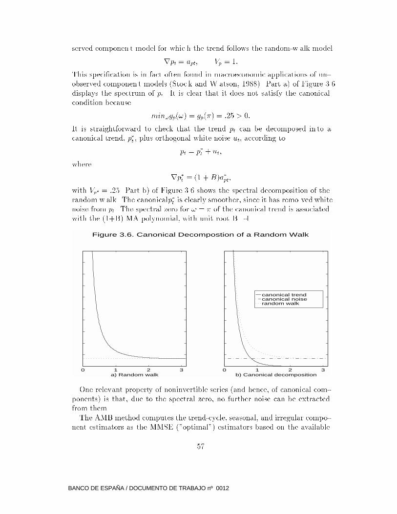
served componen t model for whic h the trend follows the random-w alk model
rpt = apt; Vp = 1:
This speci�cation is in fact often found in macroeconomic applications of un-
observed componen t models (Stoc k and W atson, 1988). Part a) of Figure 3.6
displays the spectrum of pt. It is clear that it does not satisfy the canonical
condition because
min!gp(!) = gp(�) = :25 > 0:
It is straightforward to check that the trend pt can be decomposed in to a
canonical trend, p�t , plus orthogonal white noise ut, according to
pt = p�
t + ut;
where
rp�t = (1 +B)a�pt;
with Vp� = :25. Part b) of Figure 3.6 shows the spectral decomposition of the
random w alk. The canonicalp�t is clearly smoother, since it has remo ved white
noise from pt. The spectral zero for ! = � of the canonical trend is associated
with the (1+B) MA polynomial, with unit root B=-1.
0 1 2 3a) Random walk
canonical trendcanonical noiserandom walk
Figure 3.6. Canonical Decompostion of a Random Walk
0 1 2 3b) Canonical decomposition
One relevant property of noninvertible series (and hence, of canonical com-
ponents) is that, due to the spectral zero, no further noise can be extracted
from them.
The AMB method computes the trend-cycle, seasonal, and irregular compo-
nent estimators as the MMSE ("optimal") estimators based on the available
57
BANCO DE ESPAÑA / DOCUMENTO DE TRABAJO nº 0012
series Xt = [x1; : : : ; xT ], as described in the previous section . Under our
assumptions, these estimators are also conditional expectations of the t ype
E(componen t j [observed series]); and they are obtained using the WK �lter.
For a series extending from t = �1 to t = 1, that follows model (3.44),
assume w e are interested in estimating a componen t, which we refer to as the
"signal" (the signal will be pt, then st, and �nally ut). Applying result (3.28)
to the model (3.46), the WK �lter for historical estimation of the trend-cycle
componen t is equal to the AGF of the model
�(B)zt = [�p(B)S]bt; bt � niid(0; Vp=Va); (3.48)
for the seasonal component it is given by the AGF of
�(B)zt = [�s(B)r2]bt; bt � niid(0; Vs=Va); (3.49)
and for the irregular componen t, by the AGF of
�(B)zt = rr4bt; bt � niid(0; Vu=Va): (3.50)
Notice that this last model is the "in verse" model of (3.44), which is assumed
known. Also invertibility of (3.44) guarantees stationarity of the models in
(3.48)-(3.50), and hence the three WK �lters will con verge in B and in F.
For a �nite realization, as already men tioned, the optimal estimator of the
signal is equal to the WK �lter applied to the a vailable series extended with
optimal forecasts and bac kcasts, obtained with (3.44). This is done with the
Burman-Wilson algorithm referred to in the previous section.
The following �gures illustrate the procedure. Figure 3.7 shows the spectrum
of a particular case of model (3.44) and its spectral decomposition in to trend,
seasonal, and irregular componen ts. The trend captures the peak around! =
0, and the seasonal componen t the peaks around the seasonal frequencies.
Figure 3.8 displays the WK �lters to obtain the historical estimates of the SA
series, trend, seasonal and irregular componen ts. From �gures 3.8a and b, it is
seen, for example, that the concurren t estimator of the SA series requires man y
more periods to con verge to the historical one than that of the trend. Figure 3.9
shows the squared gains of the WK �lter (see Section 2.6), that is, whic h part
of the series variation is passed to, or cut-o� from, eac h component. As seen
in 3.9c, to estimate the irregular componen t only the frequencies of no interest
for the trend or seasonal component will be employed. Figure 3.10a exhibits
a time series of 100 observations generated with the model of Figure 3.7a,
and �gures 3.10b,c and d the estimates ntj100; ptj100 and stj100(t = 1; : : : ; 100)
of the trend, seasonal, and irregular componen ts. Figure 3.11 presents the
standard errors of the estimates of Figure 3.10, mo ving from concurrent to
�nal estimator. The trend estimator con verges in a year, while the SA series
takes about 3 years for convergence. Finally, Figure 3.12 presents the forecast
function of the original series, trend and seasonal componen ts, as well as the
58
BANCO DE ESPAÑA / DOCUMENTO DE TRABAJO nº 0012

associated 90% probability intervals.
0 1 2 30
0.5
1
1.5
2
a) spectrum series0 1 2 3
0
0.5
1
1.5
2
b) spectrum trend
0 1 2 30
0.5
1
1.5
2
c) spectrum seasonal
Figure 3.7. Spectral AMB Decomposition
0 1 2 30
0.5
1
1.5
2
d) spectrum irregular
59
BANCO DE ESPAÑA / DOCUMENTO DE TRABAJO nº 0012
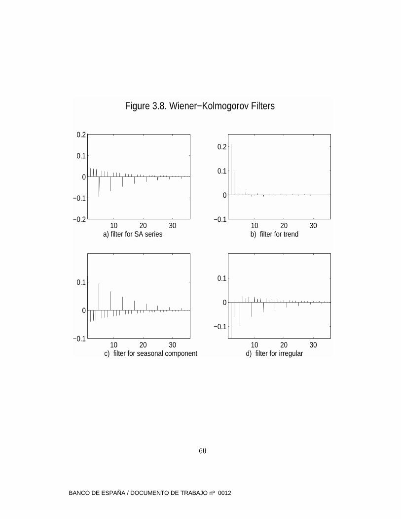
10 20 30−0.2
−0.1
0
0.1
0.2
a) filter for SA series10 20 30
−0.1
0
0.1
0.2
b) filter for trend
10 20 30−0.1
0
0.1
c) filter for seasonal component
Figure 3.8. Wiener−Kolmogorov Filters
10 20 30
−0.1
0
0.1
d) filter for irregular
60
BANCO DE ESPAÑA / DOCUMENTO DE TRABAJO nº 0012
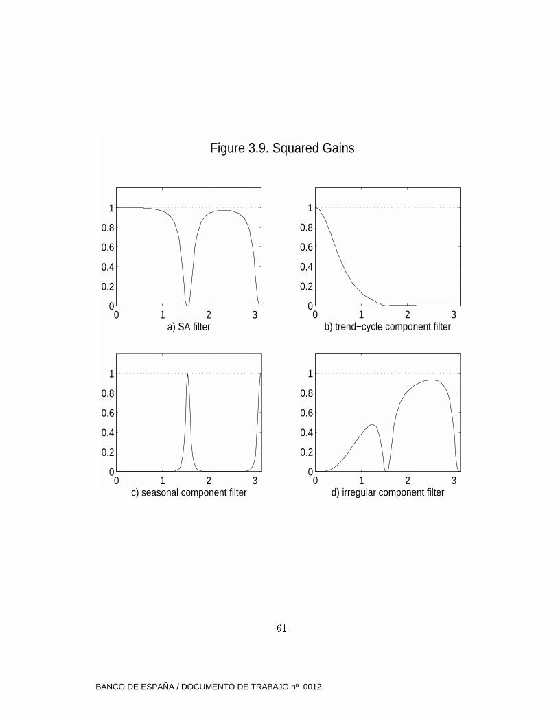
0 1 2 30
0.2
0.4
0.6
0.8
1
d) irregular component filter0 1 2 3
0
0.2
0.4
0.6
0.8
1
c) seasonal component filter
0 1 2 30
0.2
0.4
0.6
0.8
1
b) trend−cycle component filter
Figure 3.9. Squared Gains
0 1 2 30
0.2
0.4
0.6
0.8
1
a) SA filter
61
BANCO DE ESPAÑA / DOCUMENTO DE TRABAJO nº 0012
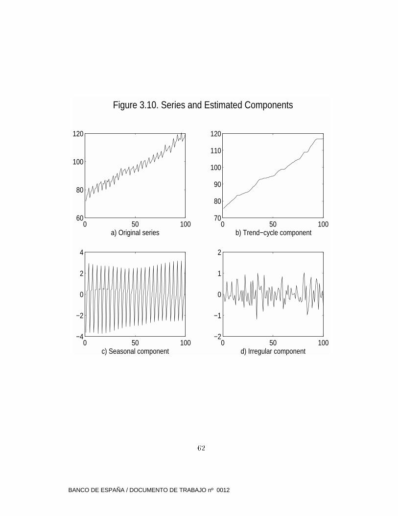
0 50 10070
80
90
100
110
120
b) Trend−cycle component0 50 100
60
80
100
120
a) Original series
0 50 100−4
−2
0
2
4
c) Seasonal component
Figure 3.10. Series and Estimated Components
0 50 100−2
−1
0
1
2
d) Irregular component
62
BANCO DE ESPAÑA / DOCUMENTO DE TRABAJO nº 0012
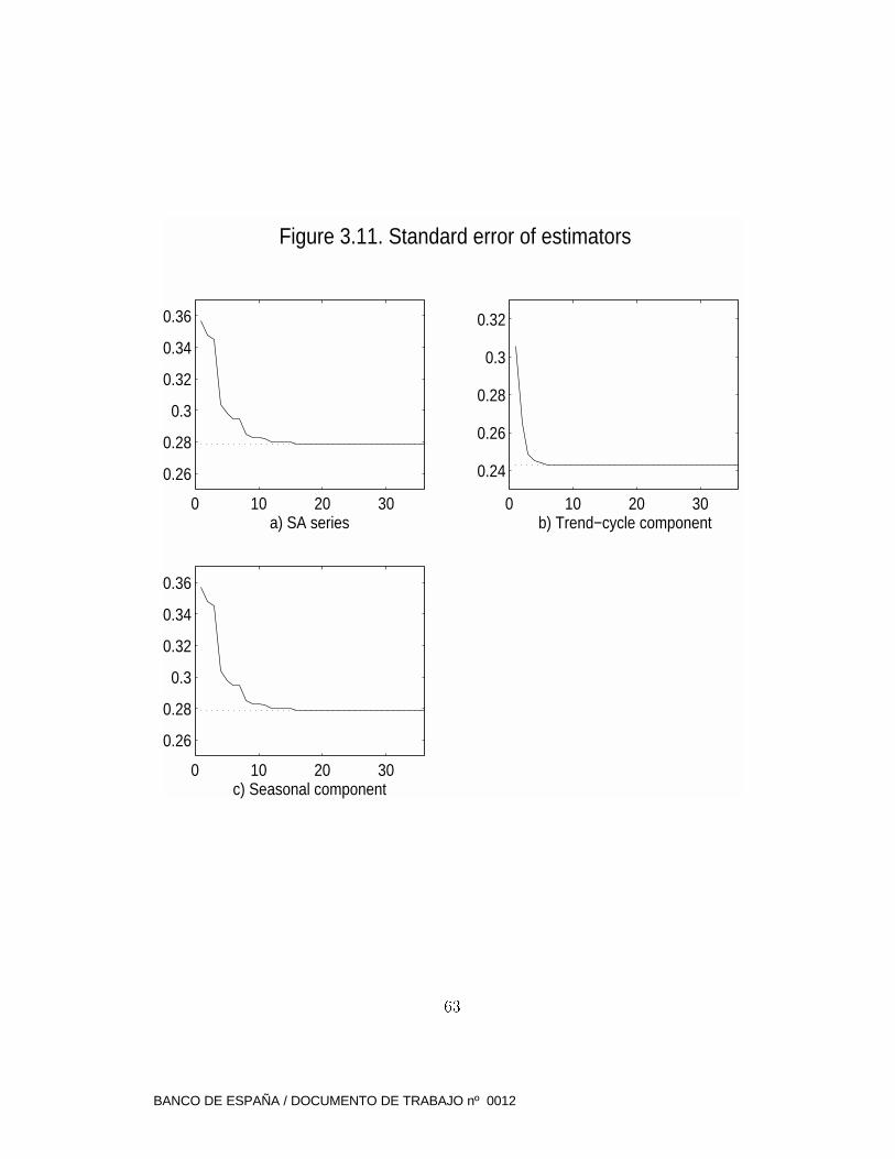
0 10 20 30
0.26
0.28
0.3
0.32
0.34
0.36
a) SA series0 10 20 30
0.24
0.26
0.28
0.3
0.32
b) Trend−cycle component
Figure 3.11. Standard error of estimators
0 10 20 30
0.26
0.28
0.3
0.32
0.34
0.36
c) Seasonal component
63
BANCO DE ESPAÑA / DOCUMENTO DE TRABAJO nº 0012
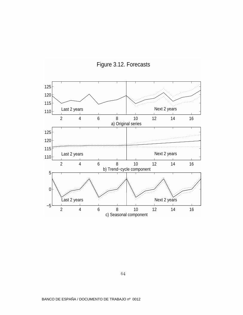
2 4 6 8 10 12 14 16
110
115
120
125
a) Original series
Last 2 years Next 2 years
2 4 6 8 10 12 14 16
110
115
120
125
b) Trend−cycle component
Last 2 years Next 2 years
Figure 3.12. Forecasts
2 4 6 8 10 12 14 16−5
0
5
c) Seasonal component
Last 2 years Next 2 years
64
BANCO DE ESPAÑA / DOCUMENTO DE TRABAJO nº 0012
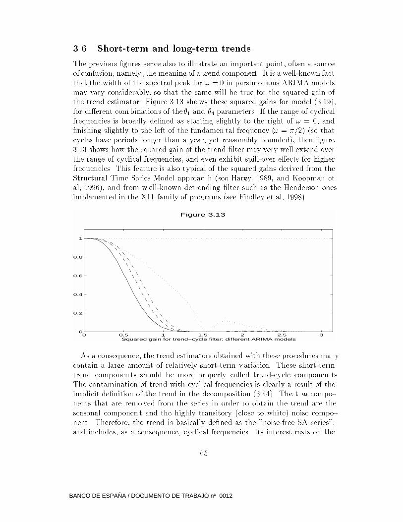
3.6 Short-term and long-term trends
The previous �gures serve also to illustrate an important point, often a source
of confusion, namely, the meaning of a trend component. It is a well-known fact
that the width of the spectral peak for ! = 0 in parsimonious ARIMA models
may vary considerably, so that the same will be true for the squared gain of
the trend estimator. Figure 3.13 shows these squared gains for model (3.19),
for di�erent combinations of the�1 and �4 parameters. If the range of cyclical
frequencies is broadly de�ned as starting slightly to the right of ! = 0, and
�nishing slightly to the left of the fundamen tal frequency (! = �=2) (so that
cycles have periods longer than a year, yet reasonably bounded), then �gure
3.13 shows how the squared gain of the trend �lter may very well extend over
the range of cyclical frequencies, and even exhibit spill-over e�ects for higher
frequencies. This feature is also typical of the squared gains derived from the
Structural Time Series Model approac h (see Harvey, 1989, and Koopman et
al, 1996), and from w ell-known detrending �lter such as the Henderson ones
implemented in the X11 family of programs (see Findley et al, 1998).
Figure 3.13
0 0.5 1 1.5 2 2.5 30
0.2
0.4
0.6
0.8
1
Squared gain for trend−cycle filter: different ARIMA models
As a consequence, the trend estimators obtained with these procedures ma y
contain a large amount of relatively short-term variation. These short-term
trend componen ts should be more properly called trend-cycle componen ts.
The contamination of trend with cyclical frequencies is clearly a result of the
implicit de�nition of the trend in the decomposition (3.44). The t wo compo-
nents that are remo ved from the series in order to obtain the trend are the
seasonal componen t and the highly transitory (close to white) noise compo-
nent. Therefore, the trend is basically de�ned as the "noise-free SA series",
and includes, as a consequence, cyclical frequencies. Its interest rests on the
65
BANCO DE ESPAÑA / DOCUMENTO DE TRABAJO nº 0012

belief that noise, unrelated to the past and to the future, is more disturbing
than helpful in short-term monitoring of the series. (In fact, SA series and
trend-cycle componen ts for short-term indicators are both pro vided at several
data-producing agencies; see Eurostat, 1999, and Bank of Spain, 1999.) A
discussion of short-term trends is con tained in Mara vall (1993).
Another importan t area where trends are used is business-cycle analysis.
Here, the trend is also de�ned as the detrended and SA series, but the concept
of detrending is rather di�erent. The aim is to remo ve a long-term trend that
does not include mo vements with periods shorter than a certain number of
years (roughly, the cutting point is set within the range 8 to 10 years). Having
de�ned the band in the frequency range associated with cyclical oscillations
(for example, those with period bet ween 2 and 10 years), the issue is to de-
sign a "band-pass" �lter that permits only the passage of frequencies within
that band. Linear �lters can only do this job in an approximate manner be-
cause the �rst derivative with respect to ! of their squared gain function is
everywhere well de�ned, and cannot take the form of an exact rectangle, with
base the frequency band pass, and height one. The Butterworth family of
�lters were designed to approximate this band-pass features. One of the mem-
bers of the family is v ery well-known in economics, where it is usually called
the Hodrick-Prescott (HP) �lter (see Hodric k and Prescott, 1980, or Prescott,
1986). Despite the fact that business cycle estimation is basic to the conduct of
macroeconomic policy and to monitoring of the economy, man y decades of ef-
fort have shown that formal modelling of economic cycles is a frustrating issue.
As a consequence, applied work and research at economic-policy related insti-
tutions has relied (and still relies) heavily on "ad-hoc" band-pass �lters and, in
particular, in the HP one. One can sa y that HP �ltering of X11-SA series has
become the presen t paradigm for business-cycle estimation in applied w ork.
Figure 3.14 represents, for the example of the previous section, the short-term
trend (or trend-cycle componen t) obtained with the AMB approac h, and the
long-term trend obtained with the HP-X11 �lter. P art a) compares the two
squared gains, and part b) the two estimated trends. The short-term c haracter
of the AMB trend and the long-term c haracter of the X11-HP trend are clearly
discernible.
If business-cycle analysts complain that series detrended with short-term
trends, of the type obtained in the AMB approach, contain very little cycli-
cal information, ad-hoc �xed �lters to estimate long-term trends are criticized
because the trends they yield could be spurious. As seen in Kaiser and Mar-
avall (2000), however, the two types of trends are not in contradiction and
can be instead quite complemen tary. When properly used, their mixture can
incorporate the desirable features of the ad-hoc design, with a sensible and
complete model-based structure, that fully respects the features of the series
66
BANCO DE ESPAÑA / DOCUMENTO DE TRABAJO nº 0012
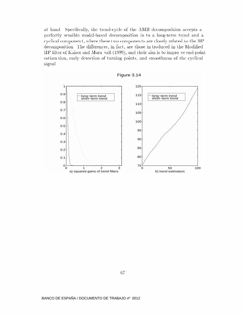
at hand. Speci�cally, the trend-cycle of the AMB decomposition accepts a
perfectly sensible model-based decomposition in to a long-term trend and a
cyclical componen t, where these two componen ts are closely related to the HP
decomposition. The di�erences, in fact, are those in troduced in the Modi�ed
HP �lter of Kaiser and Mara vall (1999), and their aim is to impro ve end-point
estiam tion, early detection of turning points, and smoothness of the cyclical
signal.
long−term trend short−term trend
0 1 2 30
0.1
0.2
0.3
0.4
0.5
0.6
0.7
0.8
0.9
1
a) squared gains of trend filters
long−term trend short−term trend
Figure 3.14
0 50 10075
80
85
90
95
100
105
110
115
120
b) trend estimators
67
BANCO DE ESPAÑA / DOCUMENTO DE TRABAJO nº 0012
4 References
Banco de Espa~na (1999), Bolet��n Econ�omico, mon thly bulletin, Madrid:
Banco de Espa~na.
Bell, W.R. (1984), \Signal Extraction for Nonstationary Time Series", An-
nals of Statistics 12, 646-664.
Bell, W.R. and Hillmer, S.C. (1991), \Initializing the Kalman Filter
for Nonstationary Time Series Models", Journal of Time Series A nalysis12,283-300.
Box, G.E.P. and Jenkins, G.M. (1970), Time Series A nalysis: Forecasting
and Control, San Francisco: Holden-Day.
Box, G.E.P., Hillmer, S.C. and Tiao, G.C. (1978), \Analysis and Mod-
eling of Seasonal Time Series", in Zellner, A. (ed.), Seasonal Analysis of Eco-nomic Time Series, Washington, D.C.: U.S. Dept. of Commerce- Bureau of
the Census, 309-334.
Box, G.E.P. and Tia o, G.C.(1975), \ Intervention Analysis with Appli-
cations to Economic and En viromen tal Problems",Journal of the AmericanStatistical Association 70, 71-79.
Brockwell,P. and D avis, R.(1987), Time Series: The ory ans Metho ds,
Berlin: Springer-Verlag.
Burman, J.P. (1980), \Seasonal Adjustment by Signal Extraction", Journal
of the Royal Statistical Society A 143, 321-337.
Burridge, P. and W allis, K.F.(1984), \Unobserved Componen t Models
for Seasonal Adjustmen t Filters",Journal of Business and Economic Statistics
2, 350-359.
Chen, C. and Liu, L.M. (1993), \Joint Estimation of Model P arameters and
Outlier E�ects in Time Series", Journal of the American Statistical Association88, 284-297.
De Jong, P. (1991), \The Difusse Kalman Filter", Annals of Statistics 19,
1073-1083.
EUROSTAT(1999), Monthly Panor ama of European Business, Luxembourg:
O�cial Publications of the European Communities.
Findley, D.F., Monsell, B.C., Bell, W.R., Otto, M.C. and Chen,
B.C. (1998), \ New Capabilities and Methods of the X12 ARIMA Seasonal
Adjustmen t Program" (with discussion),Journal of Business and EconomicStatistics, 16, 127-177.
68
BANCO DE ESPAÑA / DOCUMENTO DE TRABAJO nº 0012
Fischer, B. and Planas, C. (1998) \Large Scale Fitting of ARIMA Mod-
els and Stylized Facts of Economic Time Series" Eurostat Working Paper
9/1998/A/8. To appear inThe Journal of O�cial Statistics.
Goldberg, S. (1967), Introduction to Di�erence Equations, New York: J.
Wiley and Sons.
G�omez, V. (1999), \Three Equivalent Methods for Filtering Nonstationary
Time Series". Journal of Business and Economic Statistics 17, 109-116.
G�omez, V. and Mara vall, A. (2000a), \Automatic Modelling Methods
for Univariate Series", W orking Paper 9808, Research Departmen t, Bank of
Spain. To appear as Ch.7 in Pe~na D., Tiao G.C. and Tsa y, R.S. (eds.) A
Course in Advanced Time Series A nalysis, New York: J. Wiley and Sons.
G�omez, V. and Mara vall, A. (2000b), \Seasonal Adjustmen t and Signal
Extraction in Economic Time Series". Working Paper 9809, Research Depart-
men t, Bank of Spain. To appear as Ch.8 in Pe~na D., Tiao G.C. and Tsa y, R.S.
(eds.) A Course in Advanced Time Series A nalysis, New York: J. Wiley and
Sons.
G�omez, V. and Mara vall, A.(1996), \Programs TRAMO and SEATS;
Instructions for the User" (with some updates). W orking Paper 9628, Research
Departmen t, Banco de Espa~na.
G�omez, V. and Mara vall, A.(1994), \Estimation, Prediction and In-
terpolation for Nonstationary Series with the Kalman �lter", Journal of theAmerican Statistical Association89, 611-624.
G�omez, V. and Mara vall, A.(1993), \Initializing the Kalman �lter with
Incompletely Speci�ed Initial Conditions" in Chen, R. (ed.) ApproximateKalman Filter (Series on Appr oximation and De composition), London: W orld
Scienti�c Publ. Co. 39-62.
Gourieroux, C. and Monf ort, A.(1990), S�eries Temporelles et Mo d�elesDynamiques, Paris: Economica.
Granger, C.W.J. and Newbold, P. (1986) Forecasting Economic Time
Series, New York: Academic Press.
Grenander, U. and R osenblatt, M. (1957), Statistical Analysis of Sta-tionary Time Series, New York: John Wiley .
Harvey, A.C. (1993), Time Series Mo dels, Deddington: Philip Allan.
Harvey, A.C. (1989), Forecasting Structural Time Series and the KalmanFilter, Cambridge: Cam bridge University Press.
69
BANCO DE ESPAÑA / DOCUMENTO DE TRABAJO nº 0012

Hatanaka, M. and Suzuki, M. (1967), \ A Theory of the Pseudospec-
trum and its Application to Nonstationary Dynamic Econometric Models",
in Shubik, M. (ed.), Essays in Mathematical Economics in Honor of Oskar
Mor genstern, Princeton, N.J.: Princeton Univ ersity Press.
Hendry, D.F. (1995), Dynamic Ec onometrics, Oxford: Oxford Univ ersity
Press.
Hillmer, S.C. and Tia o, G.C.(1982), \An ARIMA-Model Based Ap-
proach to Seasonal Adjustmen t",Journal of the American Statistical Associ-
ation 77, 63-70.
Hillmer, S.C., Bell, W.R. and Tiao, G.C. (1983), \Modelling Consid-
erations in the Seasonal Adjustmen t of Economic Time Series", in Zellner,
A. (ed.), Applied Time Series A nalysis of Economic Data, Washington, D.C.:
U.S. Departmen t of Commerce-Bureau of the Census, 74-100.
Hodrick, R. and Prescott, E.C. (1980), \Post-war U.S. Business Cycles:
An Empirical In vestigation", mimeo, Carnegie-Mellon University, Pittsburgh,
P.A.
Jenkins, G.M. and Watts, D.G. (1968), Spectral Analysis and its Appli-cations, San Francisco: Holden Day.
Kaiser, R. and Mara vall, A (2000), Me asuring Business Cycles in Eco-
nomic Time Series, Lectures Notes in Statistics. Springer Verlag NY. Forth-
coming.
Kaiser, R. and Mara vall, A(1999), \Estimation of the Bussines Cycle:
a Modi�ed Hodric k-Prescott �lter",Spanish Economic R eview1, 175-206.
Kohn, R. and Ansley, C.F (1986), \Estimation, Prediction, and In ter-
polation for ARIMA Models with Missing Data", Journal of the American
Statistical Association 81, 751-761.
Koopman, S.J., Harvey, A.C., Doornik, J.A. and Shephard, N.
(1996), Stamp: Structural Time Series A nalyser, Mo deller and Predictor,Lon-
don: Chapman and Hall.
Mara vall, A.(2000), \An application of TRAMO and SEATS", Working
Paper 9914, Research Departmen t, Bank of Spain. To appear in Seasonal
Adjustment Procedures. Experiences and Perspectives, Rome, ISTAT.
Mara vall, A.(1999), \Short-Term Analysis of Macroeconomic Time Series".
in A. Gerard-V aret and A Kirman (eds.),Economics: Beyond the Milennium,
Oxford: Oxford Univ ersity Press.
Mara vall, A.(1995), \Unobserved Componen ts in Economic Time Series",
in Pesaran, H. and Wic kens ,M. (eds.),The Handbook of Applied Econometrics,
vol. 1, Oxford: Basil Blac kwell.
70
BANCO DE ESPAÑA / DOCUMENTO DE TRABAJO nº 0012
Mara vall, A.(1993), \Stochastic Linear Trends: Models and Estimators",
Journal of Econometrics 56, 5-37.
Mara vall, A.(1988), \A Note on Minim umMean Squared Error Estimation
of Signals with Unit Roots", Journal of Economic Dynamics and Contr ol12,589-593.
Mara vall, A.(1985), "On Structural Time Series Models and the Charac-
terization of Componen ts",Journal of Business and Economic Statistics 3, 4,
350-355. Reprinted in Harvey, A.C. (ed.),Time Series, Cheltenham: Edw ard
Elgar Publ., 1994.
Mara vall, A. and Pier ce, D.A.(1987), "A Prototypical Seasonal Ad-
justmen t Model", Journal of Time Series A nalysis 8, 177-193. Reprinted in
Hylleberg, S. (ed.), Mo delling Seasonality, Oxford Univ ersity Press, 1992.
Mara vall, A. and Planas, C.(1999), \Estimation Error and the Spec-
i�cation of Unobserved Componen t Models", Journal of Econometrics, 92,325-353.
Mills, T.C. (1990), Time Series T echniques for Economists, Cambridge:Cambridge University Press.
Morf, M., Sidhu, G.S. and Kailath, T. (1974), \Some New Algorithms
for Recursive Estimation on Constan t, Linear, Discrete-Time Systems",IEEETransactions on Automatic Contr ol, AC 19, 315-323.
Newbold, P. (1983), \Model Chec king in Time Series Analysis", in A. Zellner
(ed.) Applied Time Series A nalysis of Economic Data, Washington, D.C.: U.S.
Departmen t of Commerce-Bureau of the Census, 133-143.
Pierce, D.A. (1979), \Signal Extraction Error in Nonstationary Time Se-
ries", Annals of Statistics 7, 1303-1320.
Pierce, D.A. (1978), \Seasonal Adjustmen t when Both Deterministic and
Stochastic Seasonality are Present", in Zellner, A. (ed.), Seasonal Analysis of
Economic Time Series, Washington, D.C.: U.S. Dept. of Commerce-Bureau
of the Census, 242-269.
Planas, C. (1997), Applied Time Series A nalysis. Mo delling, Forecasting,
Unobserved Components, and the Wiener-Kolmo gorov Filter: Luxembourg Of-
�ce for O�cial Publications of the European Communities.
Prescott, E. (1986), \Theory ahead of Business CycleMeasuremen t",Carnegie-Rochester Conference Series on Public Policy 25, 11-66.
Shiskin, J., Young, A.H. and Musgrave, J.C. (1967), \The X11 Variant
of the Census Method II Seasonal Adjustmen t Program", Technical Paper, 15,
W ashington, D.C.: Bureau of the Census.
71
BANCO DE ESPAÑA / DOCUMENTO DE TRABAJO nº 0012
Stock, J.H. and W atson, M.W.(1988), \ Variable Trends in Economic
Time Series", Journal of Economic Perspectives 2, 147-174.
Tiao, G.C. and Tsa y, R.S.(1989), \Model Speci�cation in Multiv ariate
Time Series", Journal of the Royal Statistical Society B, 51, 132-141.
Tiao, G.C. and Tsa y, R.S.(1983), \Consistency Properties of Least Squares
Estimates of Autoregressive Parameters in ARMA Models", The Annals of
Statistics 11, 856-871.
Whittle, P. (1963), Prediction and Regulation by Linear Least-Squares Meth-
ods, London: English Universities Press.
72
BANCO DE ESPAÑA / DOCUMENTO DE TRABAJO nº 0012