NOTES ON THE MODULI SPACE OF STABLE

QUOTIENTS

Dragos Oprea1

1Partially supported by NSF grants DMS-1001486, DMS 1150675 and the Sloan Foundation.

2

Outline

These notes are based on lectures given at CRM Barcelona for the course “Compactifying Moduli

Spaces” in May 2013.

We consider here compactifications of the space of maps from curves to Grassmannians

and to related geometries. We focus on sheaf theoretic compactifications via Quot scheme-type

constructions. An underlying theme is the geometric description of such compactifications, as

well as the comparison of the intersection theoretic invariants arising from these.

We divided the notes into four parts, roughly summarized as follows:

• Section 1. We study the space of morphisms from a fixed domain curve to Grassmannians

G(r, n). Two classical compactifications are available: one via stable maps and another via

Grothendieck’s Quot scheme. The two compactifications cannot be compared in general:

their boundaries are different. Nonetheless, both spaces are virtually smooth and carry com-

patible virtual fundamental classes. As a result, we can define counting invariants of mor-

phisms from fixed curves into G(r, n). The exact expressions are given by Vafa-Intriligator

type formulas, which we discuss.

• Section 2. In Gromov-Witten theory, the domain curve is however required to vary in moduli

thus acquiring nodes. While the moduli space of stable maps remains virtually smooth, the

Quot compactification does not. To remedy this problem, a moduli space Qg,m(G(r, n), d)

of stable quotients of the trivial sheaf was introduced in [MOP], via a modification of the

Quot scheme over nodal curves.

The following properties of Qg,m(G(r, n), d) hold true:

(i) the moduli space is proper over the moduli of curves Mg,m;

(ii) the moduli space carries a 2-term perfect obstruction theory and a virtual fundamental

class[Qg,m(G(r, n), d)

]vir;

(iii) the stable quotient invariants, obtained by integrating tautological classes against the

virtual fundamental cycle, coincide with the Gromov-Witten invariants of G(r, n).

• Section 3. By item (iii) above, stable quotients provide an alternative framework for calcu-

lations in Gromov-Witten theory. The advantage over stable maps is that stable quotients

yield a more economical compactification; the ensuing localization calculations have fewer

terms. In this third section, we compare the stable quotient and stable map invariants

arising from

(i) local geometries;

(ii) hypersurface geometries, cf. [CZ].

1.1. Stable maps 3

• Section 4. Finally, we present extensions of the main construction to more general geome-

tries. As in [T], [CFKi2], [CFKi3], [CFKM] we discuss the following topics:

(i) ε-stable quotients, and wall-crossing formulas;

(ii) stable quotients to certain GIT quotients, as well as the comparison between stable

map and stable quotient invariants in this setting.

The purpose of these notes is expository. We owe a great debt to the original references,

which we often followed closely. We indicated a more extensive bibliography throughout the text

rather than in this short introduction. While we tried to present here several different aspects

related to stable quotients, there are several notable omissions, for which we apologize. In particu-

lar, we do not say anything about applications of stable quotients to the study of the tautological

ring. We refer the interested reader to [P2], [PP], [J] for these important developments.

Section 1. Morphism spaces and Quot schemes over a fixed curve

The Grassmannian G(r, n) parametrizes r-dimensional subspaces of Cn. This is the prototypical

example of a moduli space, whose intersection theory, known as Schubert calculus, is useful for

many enumerative problems. In order to develop a “quantum” version of Schubert calculus, we

consider morphisms from curves into G(r, n).

To set the stage, fix C a smooth projective curve of genus g over the complex numbers. The

moduli space Mord(C,G(r, n)) of degree d holomorphic maps

f : C → G(r, n)

is generally not compact, but two different methods of compactifying it are known:

(i) via stable maps;

(ii) via Grothendieck’s Quot schemes.

1.1 Stable maps

We describe first compactification (i),

Mord(C,G(r, n)) →MC(G(r, n), d). (1.1)

Specifically,

MC(G(r, n), d) = Mg,0(C ×G(r, n), (1, d))

is the moduli space of genus g stable maps of degree (1, d) to the target C × G(r, n). A general

member of the compactification is a morphism

h : D → C ×G(r, n)

where

4

(a) D is a connected, reduced, projective, nodal curve of arithmetic genus g;

(b) h is a morphism of degree (1, d);

(c) h is stable in the sense that every genus 0 irreducible component of D over which h is

constant contains at least 3 nodes.

Such morphisms h can be understood as follows. The domain D is obtained from C by attaching

trees of rational curves. Explicitly, there exists a distinguished main component C0 of D such

that

C0∼= C → D,

while the remaining components of D are trees of rational curves T1, . . . , Tk attached at distinct

points

x1, . . . , xk ∈ C0

in such a fashion that

D = C0 ∪ T1 ∪ . . . ∪ Tk.

The restriction of h to C0,

h|C0= h0 : C0

∼= C → C ×G(r, n)

is an isomorphism onto the first factor C (which after reparametrization we may assume to the

identity), and on the second factor G(r, n) is a given by a degree d0 morphism

f0 : C → G(r, n).

The restriction of h to Tj

h|Tj = hj : Tj → C ×G(r, n)

is the constant map equal to f0(xj) on the first factor C, and gives a morphism of degree dj > 0

into the Grassmannian G(r, n), subject to the stability condition (c). We clearly must have

d0 +

k∑j=1

dj = d.

Note that the domain D of such morphisms varies in the compactification, but the stabilization

of D is always the smooth curve C.

Inclusion (1.1) is obtained in the absence of the trees T1, . . . , Tk. Indeed, to each morphism

f : C → G(r, n) we associate its graph

hf = (1, f) : C → C ×G(r, n)

which is a stable map of degree (1, d). With the above notation, the boundary

MC(G(r, n), d) \Mord(C,G(r, n))

1.2. Quot schemes 5

can be canonically stratified. Up to isomorphisms, each stratum is covered by the product

Mord0(C,G(r, n))× (Ck \∆)×M0,1(G(r, n), d1)× . . .×M0,1(G(r, n), dk),

of a morphism space of lower degree, and Kontsevich moduli spaces of genus 0 stable maps to

Grassmannians corresponding to the trees T1, . . . , Tk. Furthermore, Ck \ ∆ denotes the set of

k-distinct points on C.

1.2 Quot schemes

Compactification (ii) is given by Grothendieck’s Quot scheme, and predates the stable morphism

space we just described. The starting point of the construction (ii) is the universal short exact

sequence over the Grassmannian

0→ E → Cn ⊗OG(r,n) → F → 0.

Any morphism f : C → G(r, n) yields by pullback an exact sequence

0→ S → Cn ⊗OC → Q→ 0

where

S = f?E, Q = f?F

such that Q has degree d and rank n − r. Furthermore, both S and Q are locally free over C.

The Quot compactification

Mord(C,G(r, n)) → QC(G(r, n), d)

is obtained by allowing the quotient Q to develop torsion. Specifically, we are parametrizing short

exact sequences

0→ S → Cn ⊗OC → Q→ 0

where Q is a coherent sheaf of degree d and rank n− r over C.

Concretely, over the smooth curve C, we can write

Q = Qlf ⊕ T

where Qlf is locally free of degree d0 ≤ d, corresponding to a morphism of degree d0 to the

Grassmannian

f0 : C → G(r, n).

The torsion sheaf has support

supp T = Σ

for a divisor Σ of degree d− d0 on the curve C. Thus the boundary of the compactification can

be stratified in such a fashion that each stratum maps to the product

Mord0(C,G(r, n))× Symd−d0(C).

6

1.3 Comparison

Unless the rank is 1, the two compactifications

MC(G(r, n), d) and QC(G(r, n), d)

cannot be compared; their boundaries are different. This is made precise in [PR] where it is shown

that in general there is no morphism between the two compactifications extending the identity

on the common open set of morphisms with smooth domains (for r 6= 1).

A comparison is however possible in rank r = 1. In this case, there is a contraction morphism

c :MC(G(1, n), d)→ QC(G(1, n), d)

constructed as follows. For any stable map

h : D → C ×G(1, n)

of degree (1, d), we can associate an exact sequence

0→ S → Cn ⊗OC → Q→ 0

yielding a point of the Quot scheme. As above, writing f0 for the restriction of h to the main com-

ponent C, and letting x1, . . . , xk be the attaching points of the degree d1, . . . , dk trees T1, . . . , Tk,

the subbundle S is a twisted pullback of the universal subbundle on the Grassmannian:

S = f?0E ⊗OC(−Σ)

where

Σ = d1x1 + . . .+ dkxk.

Clearly,

S ⊂ Cn ⊗OC

and the quotient Q takes the form

Q = f?0F ⊕OΣ.

Thus, over the boundary of MC(G(1, n), d), the contraction morphism c replaces the rational

trees T1, . . . , Tk of the domain by torsion sheaves on the main component C supported at the

attaching points.

Remark 1. In higher rank, the comparison between stable maps and stable quotients holds true

in a restricted setting. Indeed, let us write

MC(G(r, n), d) →MC(G(r, n), d)

for the subscheme consisting of balanced morphisms

h : D → C ×G(r, n).

1.3. Comparison 7

These are morphisms such that the pullback

S = h?pr?E

of the tautological subbundle on the Grassmannian splits in the most democratic way over each

(component of the) rational tail Ti of the domain D:

S|Ti = OTi(−ai)⊕`i ⊕OTi(−ai − 1)⊕(r−`i)

where ai ≥ 0 and 0 < `i ≤ r. We define a contraction morphism

c :MC(G(r, n), d) → QC(G(r, n), d)

by associating to each balanced morphism a quotient on C. Let

p : D → C0∼= C

be the morphism contracting the rational tails. For simplicity, let us assume that each Ti is

irreducible. Then, we set

S = p?(S ⊗ L),

where L → D is a line bundle with

L|C = OC(−∑i

aixi), degL|Ti = ai.

This choice of twisting ensures that S ⊗ L splits as

O⊕`iTi⊕OTi(−1)⊕(r−`i)

on each rational tail Ti, so it has no higher cohomology on Ti. The pushforward sheaf

S → C

is then a vector bundle. Its degree is found via the exact sequence

0→ S ⊗ L → S ⊗ L|C0⊕i (S ⊗ L)|Ti → ⊕i(S ⊗ L)xi → 0,

where xi are the attaching points of the tails Ti. We obtain

0→ S → S ⊗ L|C0⊕i H0(Ti, S ⊗ L)⊗ Cxi → ⊕i(S ⊗ L)xi → 0,

which immediately gives

deg S = −d.

From the exact sequence above, it is also clear that the inclusion S → Cn⊗OD yields an inclusion

S → Cn ⊗OC .

8

The association S 7→ S defines the morphism c. The case r = 1 already discussed is a special

case of this construction.

The reader may find useful an alternate way to think of the vector bundle S, cf. [PR]. Write

S0 for the restriction of the subbundle S to C0∼= C. Then

S → S0

is obtained from the following construction carried out near each node at a time:

- pick a local parameter z on C0 near each of the attaching points xi;

- pick local sections s1, . . . , s`i , s`i+1, . . . , sr of S0 = S|C0 near the node xi compatible with

the splitting

S|Ti = OTi(−ai)⊕`i ⊕OTi(−ai − 1)⊕(r−`i).

Then S → S0 is locally generated near xi by

zais1, . . . , zais`i , z

ai+1s`i+1, . . . , zai+1sr.

In any case, we will not use this description below.

1.4 Smoothness

In genus 0, the moduli space of morphisms, and its two compactifications are smooth (stacks).

However, in higher genus, both the stable map and the stable quotient compactifications may be

badly behaved: several irreducible components may exist, and their dimensions may be incorrect.

These phenomena are present when the degree is small.

Example 1. When C = P1 and r = 1, the Quot scheme QP1(G(1, n), d) is the projectivized space

of n homogeneous degree d polynomials in C[x, y],

QP1(G(1, n), d) ' Pn(d+1)−1.

Example 2. In general, when r = 1 and C has arbitrary genus, QC(G(1, n), d) parametrizes exact

sequences

0→ L→ OC ⊗ Cn → Q→ 0

where L is a line bundle of degree −d. Equivalently, dualizing, points in the space are degree d

line bundles L∨ on C together with n sections, not all zero:

OC ⊗ Cn∨ → L∨.

Let Jacd(C) be the Picard variety of degree d line bundles on C, and let

π : Jacd(C)× C → Jacd(C)

1.4. Smoothness 9

be the projection. For d sufficiently large, d ≥ 2g − 1, the push forward π?P of the Poincare line

bundle

P → Jacd(C)× C

is locally free, and its fiber over [L∨] ∈ Jacd(C) is the space H0(C,L∨) of sections of L∨. In this

case,

QC(G(1, n), d)

is smooth, and is identified with the projective bundle

P((π?P)⊕n)→ Jacd(C).

When the degree is small d < 2g − 1, this description fails, and the Quot scheme almost

always has the incorrect dimension. This example can also be used to illustrate that the morphism

space may not be dense in the compactification. For instance, the space of degree 1 morphisms

Mor1(C,P1) is empty for g 6= 0, but its compactifications are not.

Exercise 1. (cf. [St])

(i) Show that for any sheaf Q→ P1 of rank n− r and degree d, there is a short exact sequence

0→ H0(Q(−1))⊗OP1(−1)→ H0(Q)⊗OP1 → Q→ 0.

Hint: The starting point is the resolution of the diagonal ∆ → P1 × P1:

0→ OP1(−1) OP1(−1)→ OP1×P1 → O∆ → 0.

(ii) Pick identifications

H0(Q(−1)) ∼= Cd, H0(Q) ∼= Cn−r+d.

Show that a GLd×GLn−r+d bundle over QP1(G(r, n), d) can be realized as an open subset

of

Hom(Cd,Cn−r+d)⊗H0(P1,OP1(1))⊕Hom(Cn,Cn−r+d).

(iii) Show that the Quot scheme QP1(G(r, n), d) is always irreducible, smooth and calculate its

dimension.

1.4.1 Tangent-obstructions

The tangent space to the Quot scheme at a short exact sequence

0→ S → Cn ⊗OC → Q→ 0

is standardly given by

TQC(G(r, n), d) = Ext0(S,Q).

Obstructions to deformations take values in the group

Ext1(S,Q).

10

By the Riemann-Roch theorem, the expected dimension of QC(G(r, n), d) is given by

e = ext0(S,Q)− ext1(S,Q) = nd− r(n− r)(g − 1).

The expression e above is a lower bound for the dimension of the Quot scheme, with equality

only when singularities are lci.

Exercise 2. (cf. [BDW]) Show that if the degree d is large enough compared to r, n and g, the

Quot scheme is irreducible, of the expected dimension, with lci singularities.

(i) Induct on the rank r. Prove that the locus where S is a stable vector bundle is irreducible of

the correct dimension. It suffices to show that the complement has strictly smaller dimen-

sion.

(ii) Otherwise, pick a destabilizing sequence

0→ A→ S∨ → B → 0

with A stable, and B in a smaller rank Quot scheme, and count moduli.

1.4.2 Virtual fundamental classes

For arbitrary degrees, the Quot scheme may be reducible and not of the expected dimension.

However, its intersection theory can still be pursued by pairing cohomology products against a

virtual fundamental class of the expected dimension, which the Quot scheme always possesses.

This is a technical aspect which we now explain using the language of [BF].

To this end, we endow QC(G(r, n), d) with a two-term perfect obstruction theory. Key to the

construction is the cotangent complex of the Quot scheme LQ, or rather its truncation τ≥−1LQat degree −1. Explicitly, for any embedding

Q → Y

of the Quot scheme into a smooth ambient space Y , with I denoting the ideal sheaf, the relevant

truncation is quasi-isomorphic in the derived category to

τ≥−1LQ = [I/I2 → ΩY |Q].

Assume now that there exists a two term complex of vector bundles and a morphism

φ : [E−1 → E0]→ τ≥−1LQ

resolving the truncation of the cotangent complex LQ of the Quot scheme in the derived category,

in such a fashion that the induced morphisms in cohomology satisfy:

(i) h0(φ) is an isomorphism and

(ii) h−1(φ) is surjective.

1.4. Smoothness 11

These conditions then guarantee the existence of a virtual fundamental class [QC(G(r, n), d)]vir

of the expected dimension

rk E0 − rk E−1.

We refer the reader to [BF], [LT] for details regarding the construction of virtual fundamental

classes. Here we just content to say that (upon picking the resolution φ to be a map of complexes

as we certainly do below) the crux of the matter is obtaining a cone C inside the vector bundle

E1 = E∨−1, whose intersection with the zero section yields the virtual fundamental class

[QC ]vir = 0!E1

[C].

Remark 2. The above definition also makes sense relatively over a base. We will occasionally

make use of the relative concept as well (i.e. relative 2-term perfect obstruction theories).

Example 3. The prototypical example of a two-term perfect obstruction theory arises from zero

loci of sections of vector bundles. Roughly speaking, in some sense, the general case pieces together

various local pictures modeled on this situation. Concretely, assume that

V → Y

is a rank r vector bundle over a smooth manifold Y of dimension n, and s is a section of V . We

let

X = Zero(s) ⊂ Y.

If s is transverse to the zero section, then X has dimension n− r. However, this will not be the

case for arbitrary sections s. Even for nontransverse sections, the zero locus X will nonetheless

carry a virtual fundamental class [X]vir of the right dimension n − r, essentially given by the

Euler class.

To this end, note first that we have placed ourselves in the general setting described above.

Indeed, the truncation of the cotangent complex of X can be explicitly written down:

τ≥−1LX = [I/I2 → ΩY |X ],

with I denoting the ideal sheaf of X in Y . The resolution of the cotangent complex

φ : [V ∨|X → ΩY |X ]→ [I/I2 → ΩY |X ]

is obtained from the natural map V ∨ → I/I2 given by differentiating s. The normal cone

CX/Y = SpecOX

⊕d≥0

Id/Id+1

is naturally embedded in the vector bundle

V |X = SpecOX

⊕d≥0

Symd(V ∨/IV ∨)

.

12

Intersecting the cone CX/Y with the zero section of V yields the virtual fundamental class

[X]vir = 0!V [CX/Y ],

which has dimension n− r. It is known that the pushforward of the class [X]vir to Y is given by

the Euler class of V :

i?[X]vir = e(V ) ∩ [Y ].

This example also shows that the virtual fundamental class does depend on the choice of

the two-term resolution of the truncated cotangent complex. Indeed, for any other vector bundle

W → Y , we may view s as a section

s⊕ 0 ∈ H0(Y, V ⊕W )

with the same zero locus X → Y . However, the virtual fundamental class now corresponds to

the Euler class e(V ⊕W ).

Theorem 1. [MO], [CFKa] The Quot scheme QC(G(r, n), d) has a two-term perfect obstruction

theory and a virtual fundamental class

[QC(G(r, n), d)]vir

in the Chow group of the expected dimension e.

Proof. Write π for the projection map

π : QC(G(r, n), d)× C → QC(G(r, n), d),

and let

0→ S → Cn ⊗O → Q→ 0

be the universal sequence of the Quot scheme overQC(G(r, n), d)×C. The deformation-obstruction

theory of the Quot scheme is standardly given by

RHomπ(S,Q) = Rπ?Hom(S,Q). (1.2)

The equality (1.2) uses the fact that the subsheaf S is locally free. Alternatively, the reduced

Atiyah class yields a morphism in the derived category

RHomπ(S,Q)∨ → LQC(G(r,n),d)

to the cotangent complex of the Quot scheme [G].

We must show that Rπ?Hom(S,Q) can be resolved by a two step complex of vector bundles.

Indeed, let D ⊂ C be an effective divisor. Then, we have an exact sequence

0→ Hom(S,Q)→ Hom(S,Q)(D)→ Hom(S,Q)(D)|D → 0,

1.4. Smoothness 13

where by abuse of notation, the restriction of the last sheaf is over

QC(G(r, n), d)×D ⊂ QC(G(r, n), d)× C.

For sufficiently positive D, we have that

R1π?(Hom(S,Q)(D)) = 0.

Therefore,

π?(Hom(S,Q)(D))

is locally free. Since D is a collection of points, it follows that

R1π?(Hom(S,Q)(D)|D) = 0,

and that

π?(Hom(S,Q)(D)|D)

is locally free. Therefore,

Rπ?Hom(S,Q)

is represented by the two term complex of vector bundles

π?(Hom(S,Q)(D))→ π?(Hom(S,Q)(D)|D),

completing the proof.

Remark 3. It is possible to rework the above proof in a more explicit, yet equivalent language,

cf. [CFKi1], [CFKM]. Let BunC(r, d) be the moduli stack of rank r vector bundles of degree d

over the curve C. There is a natural map

µ : QC(G(r, n), d)→ BunC(r, d)

given by sending

(0→ S → Cn ⊗OC → Q→ 0) 7→ S∨.

It is known that BunC(r, d) is a smooth Artin stack of dimension r2(g − 1). The image of µ,

denoted

BunC(r, d) → BunC(r, d),

is a closed and open substack. We claim that there exists a smooth stack

Y → BunC(r, d)

and a vector bundle V → Y with a canonical section τ , such that

QC(G(r, n), d) = Zero(τ) → Y .

The virtual fundamental class of QC(G(r, n), d) is the Euler class of the bundle V → Y .

14

Indeed, let D be a sufficiently ample divisor over C so that for each bundle U in the image

of µ, we have

H1(U(D)) = 0.

The choice of D is possible from the exact sequence for S = U∨. Then, we have a short exact

sequence

0→ U → U(D)→ U(D)|D → 0.

We let

Y → BunC(r, d)

denote the total space of the bundle whose fiber over U is the space of sections

H0(U(D))⊕n.

A point of Y consists of a tuple (U, s1, . . . , sn) where the n sections yield a map

Cn ⊗OC → U(D).

Over Y , we consider the vector bundle V whose fiber over (U, s1, . . . , sn) is the vector space

H0(U(D)|D)⊕n.

The vector bundle V comes equipped with a natural section τ which sends

(U, s1, . . . , sn) 7→ (s1|D, . . . , sn|D).

The zero locus of τ consists of tuples such that the sections s1, . . . , sn of U(D) vanish on D. Thus

s1, . . . , sn must be sections of U , yielding a morphism

Cn ⊗OC → U.

There is an open substack Y where these sections generate the bundle U generically. Dualizing,

we obtain a short exact sequence in QC(G(r, n), d)

0→ S = U∨ → Cn ⊗OC → Q→ 0.

This proves that over Y , we have

Zero(τ) = QC(G(r, n), d).

It is not hard to check that the canonical resolution of the cotangent complex of QC(G(r, n), d)

given via the zero locus of τ and the resolution given in the proof of Theorem 1 coincide in the

derived category. The two constructions of the virtual class of QC(G(r, n), d) agree.

Exercise 3. Fill in the details of the above constructions of the virtual fundamental class.

1.5. Intersections 15

1.5 Intersections

In this section, we consider the virtual intersection theory of Quot schemes using the virtual

fundamental class we just constructed. This has been studied by several authors using the typical

toolkit of Gromov-Witten theory, either via degenerations of the domain curve [ST], [Ber], or via

equivariant localization [MO].

Explicitly, we will evaluate products in the Chern classes of the universal subsheaf against

the virtual fundamental class. There are two types of classes we can integrate:

(i) the a-classes

ak = ck(S∨p )

are the Chern classes of the restriction Sp of the subsheaf S to

QC(G(r, n), d)× p → QC(G(r, n), d)× C,

for p ∈ C;

(ii) the f -classes are expressed as pushforwards

fk = π?ck(S∨).

Exercise 4. (cf. [St], [O2]) Show that the cohomology of QP1(G(r, n), d) is generated by the a and

f -classes.

Hint: Recall the description of the Quot scheme in Exercise 1, or alternatively, use the

following method of Ellingsrud-Stromme [ES], [Bea]: express the class of the diagonal

∆ ⊂ QP1(G(r, n), d)×QP1(G(r, n), d)

as the Euler class of a natural vector bundle. Read off the cohomology generators from the Kunneth

decomposition of ∆ in the cohomology of the product QP1(G(r, n), d)×QP1(G(r, n), d).

Exercise 5. (i) Calculate the topological Euler characteristic of the Quot scheme QC(G(r, n), d)

using a suitable torus action. Encode the answer into a generating series∑d

χ(QC(G(r, n), d)) qd.

Hint: You may want to use the fact that for any scheme X with a C?-action

χ(X) = χ(XC?).

For a suitable torus action, the fixed loci can be expressed in terms of symmetric products of

the curve C. You may want to encode the answer into a generating series over the degree,

and then extract the correct coefficient.

16

(ii) (cf. [St]) Calculate the (generating series of) Hodge polynomials of the scheme QP1(G(r, n), d)

using a suitable torus action.

The intersection theory of a-classes is well understood. Top intersections are given in closed

form by the Vafa-Intriligator formula. To explain the results, consider the symmetric function in

r variables

J(x1, . . . , xr) = nr · x−11 · · ·x−1

r

∏1≤i<j≤r

(xi − xj)−2.

Let

u = (−1)(g−1)(r2)+d(r−1).

For any polynomial P (x1, . . . , xr) in r variables, we define the transformed polynomial

P (x1, . . . , xr) = u · P (σ1(x1, . . . xr), . . . , σr(x1, . . . , xr)),

where σ1, . . . , σr are the elementary symmetric functions in the variables x1, . . . , xr. Geomet-

rically, when evaluated at a-classes, this transformation corresponds to expressing the Chern

classes of the tautological subbundle in terms of the Chern roots. We have the following

Theorem 2. [Ber], [ST], [MO]. Let P (a1, . . . , ar) be a polynomial of weighted degree equal to the

expected dimension e of the Quot scheme. Then∫[QC(G(r,n),d)]vir

P (a1, . . . , ar) =∑

(λ1,...,λr)

(P · Jg−1

)(λ1, . . . , λr).

The sum is taken over all(nr

)tuples (λ1, . . . , λr) of distinct n-roots of 1.

Furthermore, in the large-degree regime so that the Quot scheme is irreducible of the correct

dimension, cf. Exercise 2, the intersection numbers are enumerative. To this end, consider a top

monomial

P (a1, . . . , ar) = aα11 · . . . aαrr

which we evaluate over the Quot scheme QC(G(r, n), d). For each appearance of an ai-class in

the monomial above, consider a general Schubert subvariety

S → G(r, n)

representing the Chern class ci(E∨). Then, we have the following

Theorem 3. [Ber] When QC(G(r, n), d) is irreducible of the expected dimension, the above inter-

section counts the number of degree d maps from the curve C to G(r, n) sending fixed distinct

points of C to different Schubert subvarieties of the Grassmannian in general position.

The intersection numbers appearing in Theorem 2 were written down in [I]. Mathematical

proofs have relied either on degenerations of the Quot scheme to genus zero, or on equivariant

localization.

1.5. Intersections 17

Exercise 6. Prove the Vafa-Intriligator formula for degree d = 0 using the Atiyah-Bott equivariant

localization formula with respect to a suitable torus action. (See Section 3 for a discussion of

equivariant localization.)

Exercise 7. (i) Using the Vafa-Intriligator formula calcualte the degree of the Plucker embed-

ding

G(2, n)→ P(Λ2Cn).

(ii) Using the Vafa-Intriligator formula, show that the number of lines in Pn intersecting 2(n−1)

codimension 2 linear subspaces equals the Catalan number

1

n

(2n− 2

n− 1

).

By contrast, intersections involving f -classes may not be enumerative, and explicit formulas

for them have not been explored much. Nonetheless, it would be interesting to extend the Vafa-

Intriligator formula to include all intersections of a and f classes. In general, for formal variables

y2, . . . , yr, it can be seen that we can write the intersection numbers in the form∫[QC(G(r,n),d)]vir

P (a1, . . . , ar) exp(y2f2 + . . .+ yrfr) =∑

(λ1,...,λr)

(DP · Jg−1

)(λ1, . . . , λr)

for an operator D on the space of polynomials, but its expression remains unknown. Note however

that in [MO], the operator D is determined up to first order.

Remark 4. We may ask for generalizations of the Vafa-Intriligator formula, when the curve C is

replaced by a smooth projective surface S. While the virtual fundamental class is not known to

exist for arbitrary S, nonetheless, D. Schultheis showed that

Proposition 1. [S] When S is a smooth projective simply connected surface with geometric genus

pg(S) = 0, the Quot scheme of quotients of the rank n trivial sheaf over S admits a canonical

virtual fundamental class of the expected dimension.

He furthermore calculated the resulting virtual invariants in several examples corresponding to

subsheaves of ranks 1 and 2, of degree c1 = 0, coming from the Grassmannians

G(1, 3), G(2, 8),

in the case when the virtual dimension of the Quot scheme is 0. In the general case, a Vafa-

Intriligator formula in closed form remains unknown.

Section 2. Stable quotients

In this section, we vary the curve C in moduli, in order to obtain compactifications of the space

of morphisms to G(r, n) from domain curves with at worst nodal singularities.

18

The analogue of the compactification (i) of the previous section is the moduli space of stable

maps to G(r, n)

Mg(G(r, n), d).

This compactification has traditionally been used in Gromov-Witten theory. It admits a two-term

perfect obstruction theory, and hence a virtual fundamental class. Compactification (ii) needs to

be modified in order to carry a virtual fundamental class and to be able to define invariants. The

end result is a compact moduli space of stable quotients

Qg(G(r, n), d)

which we describe below following [MOP].

2.1 Definition of stable quotients and examples

In order to arrive at the correct definition, let us make the following remarks:

(i) since we are allowing nodal domains, we need to be able to glue quotients over irreducible

components. This is easiest to achieve when we have evaluation maps at the nodes. Thus,

the quotient Q needs to be locally free at the nodes;

(ii) under normalization, the nodes become marked points. Thus, it becomes necessary to con-

sider marked domain curves. The quotient Q needs to be locally free at the markings as

well;

(iii) more importantly, having evaluation maps at the markings makes it possible to pull-back

cohomology classes from G(r, n), which we may then integrate over the moduli space;

(iv) since we are searching for a virtually smooth compactification, we re-examine the proof of

Theorem 1 in the context of nodal curves. The proof carries through, as the subbundle S

is locally free thanks to (i) and (ii).

These remarks naturally lead to the following:

Definition 1. [MOP] A quasi-stable quotient (C, p1, . . . , pm, q) is the datum of

(i) a connected, projective, reduced, nodal curve C of arithmetic genus g;

(ii) distinct markings p1, . . . , pm contained in the smooth locus of C;

(iii) a short exact sequence over C,

0→ S → Cn ⊗OCq→ Q→ 0

such that

(iv) Q is locally free at the nodes of C and at the marking p1, . . . , pm.

2.1. Definition of stable quotients and examples 19

In order to obtain a proper moduli space of finite type, we need to impose a stability

condition that will limit the number of rational components of the domain. In Gromov-Witten

theory, the stability of a map f is equivalent to the ampleness of the line bundle

ωC(p1 + . . .+ pm)⊗ f?O(1)⊗3.

For stable quotients, the role of the pullback in ampleness is different:

Definition 2. [MOP] A quasi-stable quotient is stable if the Q-line bundle

ωC(p1 + . . .+ pm)⊗ (∧rS∨)⊗ε (2.3)

is ample on C for every strictly positive ε ∈ Q.

Note that the determinant of S is well-defined since S is locally free.

Quotient stability implies 2g − 2 + m ≥ 0, as well as the semistability of the underlying

curve. Indeed, stability refers to genus 0 components P1 ∼= P ⊂ C which must satisfy:

(a) each genus 0 component P contains at least 2 nodes or markings;

(b) over each genus 0 component P with exactly 2 nodes or markings, S∨ must have positive

degree.

In other words, we do not allow terminal unmarked rational components in the domain (these are

permitted for stable maps in positive degrees). Instead, unlike stable maps, we allow for torsion

in the quotient.

We need to introduce the notion of automorphism of a stable quotient. An isomorphism of

stable quotients

φ : (C, p1, . . . , pm, q)→ (C ′, p′1, . . . , p′m, q

′)

is an isomorphism of curves

φ : C∼→ C ′

preserving the natural structures:

(i) φ(pi) = p′i for 1 ≤ i ≤ m;

(ii) the subsheaves S and φ?S′ are equal inside Cn ⊗OC .

An automorphism of a stable quotient is a self-isomorphism.

Exercise 8. (cf. [MOP]) Let (C, p1, . . . , pm, q) be a stable quotient. Show that its group of auto-

morphisms Aut(q) is finite. Is the converse true?

The definition of stable quotients in families is straightforward. A family over B consists in

a proper flat family of curves C → B with m disjoint sections

p1, . . . , pm : B → C

20

together with a B-flat family of quotients

0→ S → Cn ⊗OC → Q→ 0

whose restriction over each fiber is a stable quotient.

With these definitions understood, we obtain a proper moduli space of stable quotients.

Theorem 4. [MOP] The moduli space of stable quotients Qg,m(G(r, n), d) parameterizing the data

(C, p1, . . . , pm, 0→ S → Cn ⊗OCq→ Q→ 0),

with rank(S) = r and deg(S) = −d, is a separated and proper Deligne-Mumford stack of finite

type over C.

The construction of the moduli space as a quotient stack is standard and will be reviewed

in some detail in the next subsection following [MOP]. For now, let us just discuss first examples

and properties of the moduli space.

Remark 5. First, as already remarked in the paragraphs motivating the definition, any quotient

is locally free at the markings. As in Gromov-Witten theory, this gives rise to evaluation maps

at each marking

evi : Qg,m(G(r, n), d)→ G(r, n).

Remark 6. Furthermore, also as in Gromov-Witten theory, there are gluing maps

Qg1,m1+1(G(r, n), d1)×G(r,n) Qg2,m2+1(G(r, n), d2)→ Qg,m(G(r, n), d)

whenever

g = g1 + g2, m = m1 +m2, d = d1 + d2.

These yield quotients over nodal domains.

Remark 7. Over the moduli space there is a universal curve

π : U → Qg,m(G(r, n), d)

with m sections and a universal quotient

0→ SU → Cn ⊗OU → QU → 0.

By contrast to Gromov-Witten theory, the universal curve is not isomorphic toQg,m+1(G(r, n), d).

In general, there does not even exist a forgetful map of the form

Qg,m+1(G(r, n), d)→ Qg,m(G(r, n), d).

Indeed, we have seen in Section 1 that there is no canonical way to contract the quotient sequence

over rational tails which may become unstable by forgetting markings.

2.1. Definition of stable quotients and examples 21

Remark 8. The moduli space comes equipped with a natural stabilization map of the underlying

domain curve

Qg,m(G(r, n), d)→Mg,m.

In the absence of markings, the open locus

Qg,0(G(r, n), d) ⊂ Qg,0(G(r, n), d)

corresponding to nonsingular domains C, is simply the universal Quot scheme over the moduli

space Mg of nonsingular curves. This description fails in the presence of markings or over singular

curves, since the torsion of the quotient is not allowed to be concentrated at markings or nodes.

When this happens in the limit, the marking or node is replaced by rational components (via

blowups). Thus, the preimage of a nodal curve C under the natural stabilization morphism

consists of quotients over different models of C.

Example 4. When d = 0, we have that

Qg,m(G(r, n), 0) = Mg,m ×G(r, n).

Indeed, in this case, the bundles S and Q must be trivial, thus corresponding to a constant map

to G(r, n), and stability of the quotient implies that the underlying pointed curve is stable.

Example 5. We consider next an example in genus 1. We claim

Q1,0(G(1, n), 1) = M1,1 × Pn−1.

Indeed, given a 1-pointed stable genus 1 curve (E, p) and an element ξ ∈ Pn−1, the associated

stable quotient is

0→ OE(−p) ιξ→ Cn ⊗OE → Q→ 0

where ιξ is the composition of the canonical inclusion

0→ OE(−p)→ OE

with the line in Cn determined by ξ.

Exercise 9. (cf. [MOP]) Analogously, show that the moduli space of stable maps is

M1,0(Pn−1, 1) = M1,1 × I,

where I ⊂ Pn−1 ×G(2, n) is the incidence variety of points and lines in Pn−1.

Example 6. The moduli spaces of stable quotients of degree d > 0 to the point G(1, 1), namely

Qg,m(G(1, 1), d),

are well-defined, and yield an interesting connection with the Hassett moduli spaces of weighted

stable curves studied in [H], [LM].

22

We recall the definition of the Hassett space here. Consider a collection of rational numbers

a = (a1, . . . , am) ∈ (0, 1]m

which serve as weights for the markings.

Definition 3. [H] Let (C, p1, . . . , pm) be a reduced, connected, projective, nodal curve with possibly

non distinct smooth markings. The curve is said to be a-stable if

(i) the Q-line bundle ωC(a1p1 + . . .+ ampm) is ample;

(ii) the markings pi1 , . . . , pik are allowed to coincide if and only if

ai1 + . . .+ aik ≤ 1.

The moduli space of genus g, m-pointed a-stable curves is a proper smooth Deligne-Mumford

stack Mg,a, introduced and studied in [H].

Note that for

a1 = a2 = . . . = am = 1

we recover the definition of stable curves in Mg,m. However, relevant to our situation is the

collection of m+ d weights

a = (1, . . . , 1, ε, . . . , ε)

where m of the weights equal 1, while d of the weights equal ε ≤ 1d . The resulting moduli space is

independent of ε, and is denoted for emphasis Mg,m|d. It parametrizes nodal curves with markings

p1 . . . , pm ∪ p1, . . . , pd ∈ C

satisfying the conditions

(i) the points pi are distinct and smooth;

(ii) each marking pj is a smooth point distinct from any of the points pi.

The conditions allow the points pj and pk to coincide. Stability is given by the ampleness of

ωC(

m∑i=1

pi + ε

d∑j=1

pj)

(which in fact holds for every strictly positive ε ∈ Q). This means that

(iii) each genus 0 component of C carries at least 3 markings and nodes, out of which at least

2 are either markings of type pi or nodes.

The moduli space Qg,m(G(1, 1), d) parameterizes exact sequences

0→ S → OC → Q→ 0,

2.1. Definition of stable quotients and examples 23

where S is an ideal sheaf over C. Given a weighted stable curve

(C, p1, . . . , pm, p1, . . . , pd) ∈Mg,m|d ,

we can form a stable quotient

0→ OC(−d∑j=1

pj)→ OC → Q→ 0.

In this fashion, we obtain a morphism

φ : Mg,m|d → Qg,m(G(1, 1), d).

Matching the stability conditions, we see that the map φ induces an isomorphism of coarse moduli

spaces

Mg,m|d/Sd∼→ Qg,m(G(1, 1), d)

where the symmetric group Sd acts by permuting the markings of type pj .

Example 7. In genus 0, the topology of the moduli space Q0,2(G(1, 1), d) can be understood as

follows. The domain curve is a chain of rational components joined at nodes

C = R1 ∪R2 . . . ∪Rk

where the terminal components R1 and Rk carry the markings p1 and p2. This induces a strat-

ification by topological type, which allows for the calculation of the Poincare polynomial. The

computation was carried out in [MOP].

Exercise 10. (cf. [MOP]) Show that for d > 1 the Poincare polynomial of Q0,2(G(1, 1), d) equals

p(t) = (1 + t2)d−1.

Example 8. Similarly, in genus 1, we have

Q1,0(G(1, 1), d) ∼= M1,0|d/Sd.

In this case, there is an open stratum, corresponding smooth domain curves, and boundary strata

∆k(d1, . . . , dk) corresponding to domains which are necklaces of k rational curves

E = R1 ∪R2 ∪ . . . ∪Rk

of various positive degrees d1 + . . . + dk = d. The calculation of the Poincare polynomial was

carried out by Y. Cooper.

Exercise 11. (cf. [C])

(i) Show that the virtual Poincare polynomial of the open stratum equals

t2 + . . .+ t2d.

24

(ii) Show that for each choice of degrees d1, . . . , dk, the virtual Poincare poynomial of the bound-

ary stratum ∆k(d1, . . . , dk) is t2(d−k).

(iii) Show that Q1,0(G(1, 1), d) has no odd cohomology. Find the Poincare polynomial.

Example 9. We will show that the genus 1 unmarked stable quotients to projective space yield

a smooth moduli space Q1,0(G(1, n), d), cf. Remark 10. A general study of the geometry and

topology of Q1,0(G(1, n), d) was carried out in [C]. The following properties were established,

among others:

(i) Q1,0(G(1, n), d) has no odd cohomology;

(ii) the Picard rank of Q1,0(G(1, n), d) equals 2;

(iii) the coarse moduli scheme Q1,0(G(1, n), d) is projective, and its nef cone of divisors is found;

(iv) the canonical class of the moduli space Q1,0(G(1, n), d) is computed. The moduli space is

Fano iff n(d− 1)(d+ 2) < 20;

(v) Q1,0(G(1, n), d) is unirational.

Exercise 12. (cf. [C]) Use a suitable C?-action to prove that Q1,0(G(1, n), d) has no odd coho-

mology.

Hint: for a generic action, the fixed loci are, up to products and automorphisms,

Q0,2(G(1, 1), d) and Q1,0(G(1, 1), d)

which carry no odd cohomology.

Note that the cohomology of the moduli space of stable maps has also been considered in

recent years. For instance, it was proved in [O2] that for genus 0 stable maps to partial flag

varieties, the cohomology is generated by tautological classes. In particular, the odd cohomology

vanishes. The interplay between the stable map and the sheaf theoretic compactifications is

crucial for the argument. Furthermore, an explicit presentation of the cohomology ring for maps

to Pn is given in [MM], and expressions for the Betti numbers are found in [GeP]. The Picard

group is determined for maps to projective spaces in [P1], and for maps to flag varieties in [O1].

Exercise 13. Calculate the Picard group of the moduli space of genus 0 marked stable quotients

Q0,m(G(r, n), d).

2.2 Construction of the moduli space

Let g, m and d satisfy

2g − 2 +m+ εd > 0

for all ε > 0. Following [MOP], we will construct the moduli space Qg,m(G(r, n), d) as a quotient

stack. We follow the standard approach:

2.2. Construction of the moduli space 25

(i) we first rigidify the moduli problem by adding extra structure (e.g. the choice of a basis for

the space of sections of a natural line bundle);

(ii) next we quotient out the choices made in (i) by the natural action of a group.

To begin, fix a stable degree d quotient (C, p1, . . . , pm, q) where

0→ S → Cn ⊗OCq→ Q→ 0.

By assumption, the line bundle

Lε = ωC(p1 + . . .+ pm)⊗ (ΛrS∨)ε

is ample for all ε > 0. The genus 0 components of C must contain at least 2 nodes or markings

with strict inequality for components of degree 0. As a consequence, ampleness of Lε for ε = 1d

is enough to ensure the stability of a degree d quotient. We will fix ε = 1d throughout.

Exercise 14. (cf. [MOP]) There exists a sufficiently large and divisible integer f such that the

line bundle Lf is very ample with no higher cohomology

H1(C,Lf ) = 0.

By the vanishing of the higher cohomology, the dimension

h0(C,Lf ) = 1− g + (2g − 1 +m)f (2.4)

is independent of the choice of stable quotient. Let V be a vector space of dimension (2.4). Given

an identification

H0(C,Lf ) ∼= V,

the line bundle Lf gives an embedding

i : C → P(V),

which is well-defined up to the action of the group PGL(V). Let Hilb denote the Hilbert scheme

of curves in P(V) of genus g and degree

(2g − 1 +m)f,

equal to the degree of Lf . Each stable quotient gives rise to a point in

H = Hilb× P(V)m,

where the last factors record the locations of the markings p1, . . . , pm.

Points of H correspond to tuples (C, p1, . . . , pm). A quasi-projective subscheme H′ ⊂ H is

defined by requiring

(i) the points p1, . . . , pm are contained in C,

26

(ii) the curve (C, p1, . . . , pm) is semi-stable.

We denote the universal curve over H′ by

π : C′ → H′.

Next, we construct the π-relative Quot scheme

Quotπ(G(r, n), d)→ H′

parametrizing rank n− r degree d quotients

0→ S → Cn ⊗OC → Q→ 0

on the fibers of π. A locally closed subscheme

Q′ ⊂ Quotπ(G(r, n), d)

is further singled out by requiring

(iii) the quotient Q is locally free at the nodes and markings of C and nontrivial over the

components of C with 2 special points,

(iv) the restriction of OP(V)(1) to C agrees with the line bundle

(ω(∑

pi

))f⊗ (ΛrS∨)fε.

The action of PGL(V) extends to both schemes H′ and Q′. A PGL(V)-orbit in Q′ corre-

sponds to a stable quotient up to isomorphism. The moduli space Qg,m(G(r, n), d) is the stack

quotient

Qg,m(G(r, n), d) = [Q′/PGL(V)] .

By stability, each orbit has finite stabilizers. The quotient stack thus constructed is therefore

Deligne-Mumford.

Exercise 15. (cf. [CZ]) Formulate a suitable definition of stable quotients to a product of Grass-

mannians

G(r1, n1)× . . .G(r`, n`),

and carry out the construction of the corresponding moduli space of stable quotients

Qg,m(G(r1, n1)× . . .G(r`, n`), (d1, . . . , d`)).

2.3. Obstruction theory 27

2.3 Obstruction theory

In this section we establish the existence of the virtual fundamental class of the moduli space of

stable quotients, necessary to define intersection theoretic invariants.

Theorem 5. [MOP] The moduli space Qg,m(G(r, n), d) admits a two-term perfect obstruction

theory, and a virtual fundamental class.

Proof. This is a relative version of the proof of Theorem 1. To this end, observe the natural

forgetful morphism to the Artin stack of semistable marked curves

ν : Qg,m(G(r, n), d)→Mg,m.

The fibers of the morphism ν are open subsets of Quot schemes over semistable curves, which do

admit perfect obstruction theories as proved in Theorem 1. This shows that ν admits a relative

two-term perfect obstruction theory. Via the Appendix of [GrP], it follows that Qg,m(G(r, n), d)

carries an absolute two-term perfect obstruction theory.

Alternatively, one may argue along the fibers of the morphism

µ : Qg,m(G(r, n), d)→ Bung,m(r, d),

where

Bung,m(r, d)→Mg,m

is the smooth Artin stack of vector bundles over semistable curves. As in Section 1, it can be

seen that µ has a relative two-term perfect obstruction theory. In fact, as in Remark 3, we may

exhibit Qg,m(G(r, n), d) as the zero locus of a section of a vector bundle

V → Y

over a smooth ambient stack Y → Bung,m(r, d).

Example 10. By contrast with stable maps, the moduli space Q1,0(Pn−1, 1) of genus 1 stable

quotients to G(1, n) ∼= Pn−1, without markings, is smooth, and virtual fundamental classes are

not necessary to define invariants. Smoothness follows from the vanishing of the obstruction space

Ext1(S,Q) = 0

over any genus 1 domain curve E. The vanishing is clear for smooth curves E. When

E = R1 ∪R2 ∪ . . . ∪Rk

is a necklace of rational curves, we argue using the exact sequence

0→ Hom(S,Q)→k⊕i=1

Hom(S,Q)|Ri → T → 0

for a torsion sheaf T supported at the nodes.

28

2.4 Invariants

We already remarked that, just as in the case of stable maps, the moduli space of stable quotients

comes equipped with evaluation maps

evi : Qg,m(G(r, n), d)→ G(r, n)

at each one of the m markings. In addition, using the universal curve

π : U → Qg,m(G(r, n), d)

and its m sections s1, . . . , sm, we define the cotangent classes

ψi = s?i c1(ωπ).

These structures lead to a system of descendant invariants. Indeed, fix classes

γ1, . . . , γm ∈ H?(G(r, n))

and nonnegative integers a1, . . . , am ≥ 0. We set

〈τa1γ1, . . . , τamγm〉Q =

∫[Qg,m(G(r,n),d)]vir

m∏i=1

ψaii · ev?i γi.

The invariants without cotangent insertions are said to be primary.

Note that the same definitions are valid for the moduli space of stable maps Mg,m(G(r, n), d)

yielding the system of descendant Gromov-Witten invariants

〈τa1γ1, . . . , τamγm〉M =

∫[Mg,m(G(r,n),d)]vir

m∏i=1

ψaii · ev?i γi.

As a consequence of the matching results in the next subsection, we have the following

Corollary 1. [MOP] The stable map and stable quotient descendant invariants coincide

〈τa1γ1, . . . , τamγm〉M = 〈τa1

γ1, . . . , τamγm〉Q.

2.5 Virtually smooth morphisms and comparison of invariants

We argue that when r = 1, the virtual fundamental classes for stable maps and stable quotients

are matched under the contraction morphism

c : Mg,m(G(1, n), d)→ Qg,m(G(1, n), d).

This generalizes the contraction morphism of Section 1 defined for fixed domain curve.

Theorem 6. [MOP] We have

c?[Mg,m(G(1, n), d)]vir = [Qg,m(G(1, n), d)]vir.

2.5. Virtually smooth morphisms and comparison of invariants 29

In arbitrary rank r, the comparison of the virtual classes holds after composition with the

Plucker embedding

ι : G(r, n)→ P(ΛkCn) := P

via the diagram

Mg,m(G(r, n), d)ιM // Mg,m(P, d)

c

Qg,m(G(r, n), d)

ιQ // Qg,m(P, d).

In this case, we have

(c ιM )?[Mg,m(G(r, n), d)]vir = (ιQ)?[Qg,m(G(r, n), d)]vir.

The proof of Theorem 6 given in [MOP] relies on the virtual localization theorem of Graber-

Pandharipande [GrP], and is valid in arbitrary rank. A different proof of the theorem is outlined

below for r = 1, following Manolache [Ma1].

We begin with the following piece of terminology:

Definition 4. [Ma1] Let f : X → Y be a morphism of Deligne-Mumford stacks. Assume that Xand Y admit two-term perfect obstruction theories with resolutions

EX → LX , EY → LY ,

and that f admits a relative two-term perfect obstruction theory with resolution

EX/Y → LX/Y .

We say that f is virtually smooth, provided there is a diagram of distinguished triangles

f?EY //

EX //

EX/Y //

f?EY [1]

f?LY // LX // LX/Y // f?LY [1]

For instance, if f : X → Y admits a relative perfect obstruction theory and Y is smooth of

expected dimension, then f is virtually smooth, cf. Appendix of [GrP].

In this general setting, Manolache showed:

Theorem 7. [Ma1] Assume that f : X → Y is a virtually smooth, proper, surjective morphism of

stacks of the same virtual dimension

vir. dim. X = vir. dim. Y.

If Y is connected, then there exists an integer n such that

f?[X ]vir = n[Y]vir.

30

In particular, the pushforward of the virtual class of X is supported on the various irreducible

components of the virtual class of Y, and the component multiplicities agree.

Relevant to our context, it suffices therefore to prove that:

Theorem 8. [Ma1] The contraction morphism c : Mg,m(G(1, n), d)→ Qg,m(G(1, n), d) is virtually

smooth.

Since the two stacks are connected, of the same virtual dimension, and the virtual classes

agree over a common open subset, the Theorem yields the result

c?[Mg,m(G(1, n), d)]vir = [Qg,m(G(1, n), d)]vir.

The key to proving Theorem 8 is the exercise below, whose proof we leave to the reader.

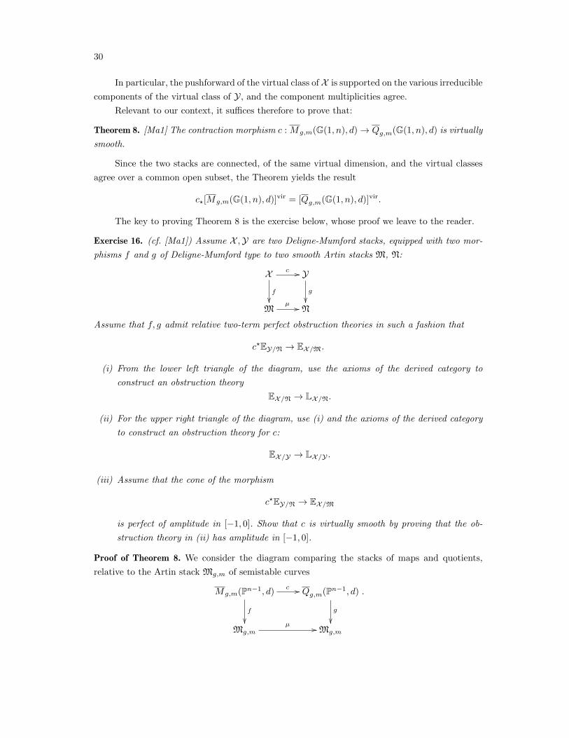
Exercise 16. (cf. [Ma1]) Assume X ,Y are two Deligne-Mumford stacks, equipped with two mor-

phisms f and g of Deligne-Mumford type to two smooth Artin stacks M, N:

X c //

f

Yg

M

µ // N

Assume that f, g admit relative two-term perfect obstruction theories in such a fashion that

c?EY/N → EX/M.

(i) From the lower left triangle of the diagram, use the axioms of the derived category to

construct an obstruction theory

EX/N → LX/N.

(ii) For the upper right triangle of the diagram, use (i) and the axioms of the derived category

to construct an obstruction theory for c:

EX/Y → LX/Y .

(iii) Assume that the cone of the morphism

c?EY/N → EX/M

is perfect of amplitude in [−1, 0]. Show that c is virtually smooth by proving that the ob-

struction theory in (ii) has amplitude in [−1, 0].

Proof of Theorem 8. We consider the diagram comparing the stacks of maps and quotients,

relative to the Artin stack Mg,m of semistable curves

Mg,m(Pn−1, d)c //

f

Qg,m(Pn−1, d)

g

Mg,m

µ //Mg,m

.

2.5. Virtually smooth morphisms and comparison of invariants 31

The morphism µ contracts the unmarked rational tails: these are disallowed for stable quotients

by stability. The relative obstruction theory of stable maps

f : Mg,m(Pn−1, d)→Mg,m

is known to be given by the complex

Ef = (Rp?(ev?TPn−1))∨

where the universal structures over the universal curve C are summarized by the diagram below

C

p

ev // Pn−1

Mg,m(Pn−1, d)

.

Similarly, the relative obstruction theory of stable quotients along the fibers of the forgetful

morphism

g : Qg,m(Pn−1, d)→Mg,m

is given by the complex

Eg = (Rπ?Hom(SU , QU ))∨,

obtained by pushforward of universal structures from the universal curve

π : U → Qg,m(Pn−1, d).

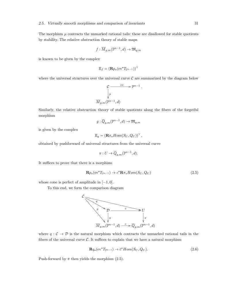
It suffices to prove that there is a morphism

Rp?(ev?TPn−1)→ c?Rπ?Hom(SU , QU ) (2.5)

whose cone is perfect of amplitude in [−1, 0].

To this end, we form the comparison diagram

Cq

&&MMMMM

MMMMMM

M

p

:::

::::

::::

::::

::

++XXXXXXXXX

XXXXXXXXXX

XXXXXXXXXX

X

D

π

c // U

π

Mg,m(Pn−1, d)

c // Qg,m(Pn−1, d)

where q : C → D is the natural morphism which contracts the unmarked rational tails in the

fibers of the universal curve C. It suffices to explain that we have a natural morphism

Rq?(ev?TPn−1)→ c?Hom(SU , QU ). (2.6)

Push-forward by π then yields the morphism (2.5).

32

We now explain how to construct (2.6). Recall that for a fixed stable map

f : C → Pn−1,

the contraction morphism

q : C → D

collapses the degree d1, . . . , dk rational tails T1, . . . , Tk of the domain C, and replaces the maps

over them by quotients with torsion over points x1, . . . , xk ∈ D. Here, we write

C = D ∪ T1 ∪ . . . ∪ Tk.

(The notation differs slightly from that of Section 1.) The resulting stable quotient over D

0→ S → Cn ⊗OD → Q→ 0

is obtained via

S = (f |D)?OPn−1(−1)⊗OD(−

k∑i=1

dixi).

As a consequence of this description, it is not hard to see that over D we have natural morphism

q?(ev?OPn−1(1))→ S∨.

This observation allows us to compare two natural exact sequences. The first sequence is obtained

over C by pullback of the Euler sequence of Pn−1:

0→ OC → ev?OPn−1(1)⊗ Cn → ev?TPn−1 → 0.

The second sequence is obtained by pullback to D from the universal stable quotient over U :

0→ OD → c?S∨U ⊗ Cn → c?Hom(SU , QU )→ 0.

Since

q?(ev?OPn−1(1))→ c?S∨U ,

comparing the two exact sequences via the pushforward by q yields the morphism claimed in

(2.6):

Rq?(ev?TPn−1)→ c?Hom(SU , QU ).

It suffices to explain that the cone of morphism (2.5) is perfect with amplitude in [−1, 0].

The amplitude is certainly contained in [−1, 1]. Furthermore, there are no terms in degree 1. This

is because the natural map

H1(C, f?TPn−1)→ H1(D,Hom(S,Q))

is surjective. Indeed, from the normalization sequence over C we obtain

0→ f?TPn−1 → (f |D)?TPn−1 ⊕k⊕i=1

(f |Ti)?TPn−1 → T → 0

2.5. Virtually smooth morphisms and comparison of invariants 33

where T is supported over the nodes x1, . . . , xk. Similarly, from the description of the quotient

S over D, we have

0→ (f |D)?TPn−1 → Hom(S,Q)→ T ′ → 0

where T ′ is torsion over D. Passing to cohomology in the first exact sequence, we find a surjection

H1(C, f?TPn−1)→ H1(D, (f |D)?TPn−1)→ .0

The second exact sequence yields the surjection

H1(D, (f |D)?TPn−1)→ H1(D,Hom(S,Q))→ 0.

The composition must be surjective as well, completing the proof of the claim.

Remark 9. Manolache’s argument also extends to higher rank, cf. [Ma2]. The details are however

more involved. We have seen in Section 1 that there is a comparison morphism

c : Mg,m(G(r, n), d) → Qg,m(G(r, n), d)

whose domain is the locus of balanced stable maps (stable maps for which the pullback of the

tautological bundle of G(r, n) to each rational tail is as balanced as possibly allowed). Unfortu-

nately, the morphism c does not extend to the entire moduli space of stable maps. To remedy

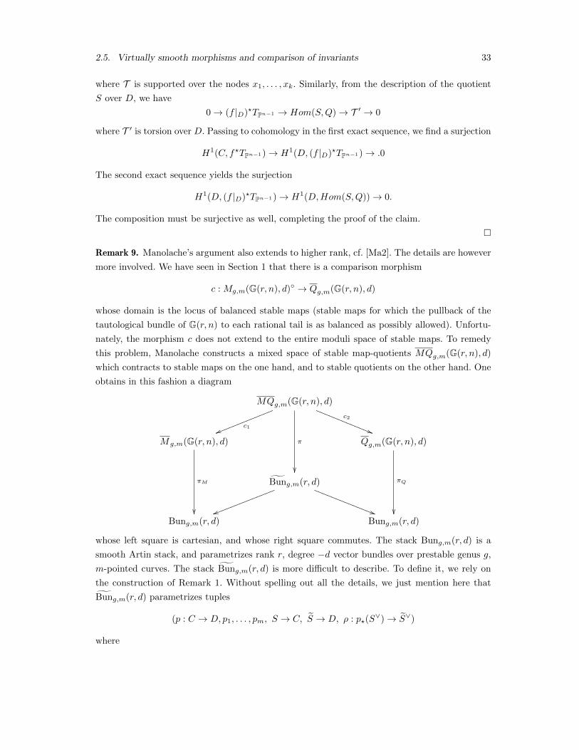
this problem, Manolache constructs a mixed space of stable map-quotients MQg,m(G(r, n), d)

which contracts to stable maps on the one hand, and to stable quotients on the other hand. One

obtains in this fashion a diagram

MQg,m(G(r, n), d)

c1uullllll

llllll

lc2

))RRRRR

RRRRRR

RR

π

Mg,m(G(r, n), d)

πM

Qg,m(G(r, n), d)

πQ

Bung,m(r, d)

uulllllll

llllll

l

))RRRRR

RRRRRR

RRR

Bung,m(r, d) Bung,m(r, d)

whose left square is cartesian, and whose right square commutes. The stack Bung,m(r, d) is a

smooth Artin stack, and parametrizes rank r, degree −d vector bundles over prestable genus g,

m-pointed curves. The stack Bung,m(r, d) is more difficult to describe. To define it, we rely on

the construction of Remark 1. Without spelling out all the details, we just mention here that

Bung,m(r, d) parametrizes tuples

(p : C → D, p1, . . . , pm, S → C, S → D, ρ : p?(S∨)→ S∨)

where

34

(i) C and D are connected, reduced, nodal, projective curves of arithmetic genus g, and p

is the morphism contracting the rational tails Ti of the domain C to points xi in D. (A

rational tail is a genus 0 tree not containing any marked points.)

(ii) p1, . . . , pm are smooth distinct points of C (which by definition cannot lie not on the

contracted tails Ti);

(iii) S is a vector bundle over C of degree −d, and S is a vector bundle over D of degree −d;

(iv) the morphism ρ is an isomorphism away from the contracted tails;

(v) ωC(p1 + . . .+ pm)⊗ (ΛrS∨)ε is ample for all ε > 2 rational;

(vi) if we denote by τ the cokernel of ρ : p?(S∨) → S∨, then for each rational tail Ti of the

domain C sitting over xi ∈ D, we have

lengthxi(τ) = deg(S∨|Ti).

The stack just described may not be irreducible, so to define Bung,m(r, d) we need to single out

the correct component (which contains contains those S’s which are balanced over the rational

tails). The construction of MQg,m(G(r, n), d) is quite similar, but we will not review it here. In

order to think about this space, the reader can refer to the cartesian left square of the diagram

above.

Using the left square, one endows the moduli space of stable map-quotients with a rel-

ative perfect obstruction theory EMQ over Bung,m(r, d), and thus with a virtual fundamental

class. Furthermore, there are comparison maps to the obstruction theories of maps and quotients

relatively to Bung,m(r, d):

c?1EM/Bun → EMQ/Bun

c?2EQ/Bun → EMQ/Bun

.

Now, it can be shown that c1 is virtually smooth. This holds in the general setup of any cartesian

square; the result is discussed in Section 5 of [K]. Crucially, Manolache proves that c2 is virtually

smooth as well. As result, we obtain

(c1)?[MQg,m(G(r, n), d)]vir = [Mg,m(G(r, n), d)]vir

(c2)?[MQg,m(G(r, n), d)]vir = [Qg,m(G(r, n), d)]vir.

The equality of invariants follows from here.

Section 3: Stable quotient invariants

In this section, we present concrete calculations of stable quotient invariants. We focus on two

types of geomeries:

3.0. Equivariant localization 35

(i) local geometries;

(ii) hypersurface geometries.

Specifically, we present a sample computation for the local fourfold OP2(−1) ⊕ OP2(−2) → P2.

Then, we explain more general results due to Cooper and Zinger, cf. [CZ].

3.0 Equivariant localization

For both geometries (i) and (ii), the invariants are calculated via equivariant localization. For the

concrete genus 0 examples we present in this section, the usual Atiyah-Bott localization suffices,

but for calculations in arbitrary genus, we require the full strength of the Graber-Pandharipande

virtual localization theorem [GrP] whose statement we recall.

Assume that Q is a moduli space equipped with the action of a torus T. Assume furthermore

that there exists a two-term torus-equivariant perfect obstruction theory

φ : [E−1 → E0]→ τ≥−1LQ.

Each one of the torus fixed loci

ji : Qi → Q

also comes equipped with a natural two-term perfect obstruction theory obtained from taking

the invariant part of the obstruction theory of Q restricted to Qi:

φi : [E inv−1 → E inv

0 ]→ τ≥−1LQi .

This yields a virtual fundamental class [Qi]vir. In a similar fashion, the moving part of the

obstruction theory yields the virtual co-normal bundle of Qi in Q:

[Emov−1 → E mov

0 ].

Dualizing, the equivariant Euler class of the virtual normal bundle is defined as

e(Nviri ) =

e((E∨0 ) mov)

e((E∨−1) mov).

The equivariant Euler class above is an invertible element in the localized equivariant cohomology

of Qi (obtained by inverting the torus characters). Crucially for our calculations, we can express

the virtual class of Q in equivariant cohomology in terms of virtual classes of fixed loci

[Q]vir =∑i

(ji)?

(1

e(Nviri )∩ [Qi]

vir

).

Consequently, for any equivariant lift of a cohomology class α, the above formula yields∫[Q]vir

α =∑i

∫[Qi]vir

j?i α

e(Nviri )

.

36

In the particular case when

Q = Zero(s)

for an equivariant section s of an equivariant vector bundle V → Y over a smooth projective

variety Y with a torus action, it is not hard to see that the virtual localization formula follows

from the usual Atiyah-Bott localization over the fixed loci Yi of Y :

[Y ] =∑i

(ji)?

(1

e(NYi/Y )∩ [Yi]

)

after intersecting with the Euler class e(V ).

Torus fixed quotients

We apply the (virtual) localization theorem to the moduli space of stable quotients. To this end,

we consider the action of the one dimensional torus T on Cn with distinct weights

w1, . . . ,wn.

This induces an action on stable quotients

0→ S → Cn ⊗OC → Q→ 0

using the torus action on the middle term.

For our purposes, it will be sufficient to describe the T-fixed loci only over the moduli space

Qg,m(G(1, n), d). These are indexed by connected decorated graphs (Γ, ν, γ, s, ε, δ, µ) where

(i) Γ = (V,E) such that V is the vertex set and E is the edge set (no self-edges are allowed);

(ii) ν : V → G(1, n)T is an assignment of a T-fixed point ν(v) to each element v ∈ V ;

(iii) γ : V → Z≥0 is a genus assignment;

(iv) for each v ∈ V , s(v) is a non-negative integer measuring the torsion of the quotient on

components;

(v) ε is an assignment to each e ∈ E of a T-invariant curve ε(e) of G(1, n) together with a

covering number δ(e) ≥ 1;

(vi) µ is a distribution of the markings to the vertices V .

subject to the compatibilities:

(a) the invariant curve ε(e) of G(1, n) joins the T-invariant points ν(v) and ν(w), where v and

w are the vertices of the edge e;

3.1. Local geometries 37

(b) we have ∑v∈V

γ(v) + h1(Γ) = g

and ∑v∈V

s(v) +∑e∈E

δ(e) = d

The T-fixed locus corresponding to a decorated graph as above is, up to a finite map, the

product of Hassett spaces indexed by the vertices in V :∏v∈V

Mγ(v), val(v)|s(v).

The valency of a vertex v counts all incident edges and markings. A description of the invariant

stable quotients is as follows. For each vertex v of the graph, pick a curve Cv in the Hassett

moduli space with markings

p1, . . . , pval(v), p1, . . . , ps(v).

For each edge e, pick a rational curve Ce. The domain C of the stable quotient is obtained by

gluing the curves Cv and Ce via the graph incidences E ⊂ V × V , and distributing the markings

on the domain via the assignment µ. The short exact sequence on C is constructed by gluing the

following quotients over the components.

(i) On the component Cv, the stable quotient is given by the exact sequence

0→ OCv (−p1 − . . .− ps(v))i→ Cn ⊗OCv → Q→ 0.

The injection i is the composition subsheaf

OCv (−p1 − . . .− ps(v)) → C⊗OCv → Cn ⊗OCv

where the second map is determined by the invariant line ν(v) in Cn.

(ii) For each edge e, consider the degree δe covering of the T-invariant curve ε(e) ∼= P1 in

G(1, n):

fe : Ce → ε(e)

ramified only over the two torus fixed points ν(v) and ν(w) of the curve ε(e). The stable

quotient is obtained pulling back the tautological sequence of G(1, n) to Ce.

3.1 Local geometries

Our first calculations concern stable quotient invariants of local geometries. We focus here on the

Calabi-Yau case. Thus, we let

π : V → G(r, n)

38

be the total space of a bundle over the Grassmannian with

detV = OG(r,n)(−n),

so that the canonical bundle of V is trivial. For instance, we may take

V = OG(r,n)(−a1)⊕ . . .⊕OG(r,n)(−ak)

where

a1 + . . .+ ak = n, ai > 0.

The canonical bundle of the Grassmannian is a special case.

To motivate the definition of the local invariants, fix a smooth curve C and assume further-

more that

(i) for any nonconstant morphism h : C → G(r, n), the pullback bundle h?V has no nonzero

global sections.

Consider a morphism f : C → V to the total space of V . By assumption (i), f is determined by

the composition

h : C → G(r, n), h = π f

hence the space of maps of fixed degree to V and G(r, n) coincide. However, the obstruction

theories of the moduli spaces differ by a nontrivial vector bundle with fibers

W = H1(C, h?V )

whose dimension is constant by assumption (i). Indeed, the tangent-obstruction spaces for the

two moduli spaces are

Hi(C, f?TV ) and Hi(C, h?TG(r,n)), 0 ≤ i ≤ 1,

respectively. From the exact sequence

0→ h?V → f?TV → h?TG(r,n) → 0

we see that

0→ H0(C, f?TV )→ H0(C, h?TG(r,n))→ H1(C, h?V )→ H1(f?TV )→ H1(h?TG(r,n))→ 0.

Therefore, the corresponding virtual classes of maps to V and G(r, n) differ by the Euler class of

W:

[Mor(C, V )]vir = e(W) ∩ [Mor(C,G(r, n))]vir.

For the special case

V = OG(r,n)(−a1)⊕ . . .⊕OG(r,n)(−ak),

3.1. Local geometries 39

the bundle W has fibers

H1(C, h?O(−a1))⊕ . . .⊕H1(C, h?O(−ak)).

Since h?O(−1) = detS, this motivates the following definition of the virtual class of the stable

quotient invariants to the bundle V :

[Qg,m(V, d)]vir = e(R1π? ((detSU )a1 ⊕ . . .⊕ (detSU )ak)) ∩ [Qg,m(G(r, n), d)]vir,

where as before

0→ SU → Cn ⊗OU → QU → 0

is the universal sequence of Qg,m(G(r, n), d) over the universal curve U .

Example 11. For example consider the conifold, the total space of

OP1(−1)⊕OP1(−1)→ P1.

Just as in Gromov-Witten theory, we define the conifold invariants

Ng,d =

∫[Qg,0(P1,d)]vir

e(R1π∗(SU )⊕R1π∗(SU ))

for g ≥ 1. In genus 0, we need to modify the definition slightly because the moduli space

Q0,0(P1, d) is not defined. Adding two markings is necessary for the stability condition to be

non-vacuous. We set

N0,d =1

d2

∫[Q0,2(P1,d)]vir

e(R1π∗(SU )⊕R1π∗(SU )) · ev?1H · ev?2H.

The ensuing series in degree 1

F (t) = 1 +∑g≥1

Ng,1t2g

agrees with the calculation of Gromov-Witten invariants over the moduli space of maps.

Proposition 2. [MOP] The local invariants Ng,d are determined by the following two equations

Ng,d = d2g−3Ng,1,

F (t) =

(t/2

sin(t/2)

)2

.

Example 12. There are other Calabi-Yau geometries to consider. Here, we present the case of the

local fourfold

Y = O(−1)⊕O(−2)→ P2,

which was not included in [MOP]. This computation may be skipped on a first reading, but

we refer to [Z2] and [CFKi3] for more general results. For dimension reasons, invariants can be

40

defined only in genus 0 and 1. We let P and H denote the point and hyperplane class on P2. The

invariants

N0,d(P,H) =

∫Q0,2(P2,d)

e(R1π?SU ⊕R1π?S2U ) · ev?1P · ev?2H (3.7)

N1,d =

∫Q1,0(P2,d)

e(R1π?SU ⊕R1π?S2U ) (3.8)

agree with the Gromov-Witten theory calculation of Klemm-Pandharipande [KP].

Proposition 3. We have

N0,d(P,H) =(−1)d

2d

(2d

d

),

N1,d =(−4)d

24d.

Proof. The integral (3.7) is computed by equivariant localization using different choices of equiv-

ariant lifts. In the situation at hand, the full strength of the virtual localization theorem is not

necessary, since we are working over a smooth stack.

We let the one dimensional torus T act on P2 with weights 0,w1,w2, and fixed points

P0, P1, P2.

(Note that the markings of the domain of the quotient are similarly denoted by small cap p’s,

but for the fixed points over P2 we use capital letters. We hope that this notation will not cause

confusion below.) For simplicity of notation, we let

w = w1 − w2.

In the integrand, the torus T naturally acts on

SU → C3 ⊗OU .

We endow the bundle S2U with the natural action twisted by a trivial line bundle with weight

−w1 − w2. This twist is inspired from calculations in Gromov-Witten theory.

Our choice of equivariant weights forces the following constraints on the localization graphs

that give nonvanishing contributions:

(i) there is no node of the domain mapping to P0 – such a node would yield a weight zero

summand in H1(SU ). Similarly, the second marking cannot map to P0;

(ii) no edge joining P1 and P2 can appear in a localization graph – such an edge would produce

a zero weight summand in H1(S2U ).

For instance, to explain (ii), consider a T-invariant stable quotient with domain curve C. Let

Cv and Ce denote the components of domain, and let ni denote the nodes. We have an exact

sequence

0→ S →⊕v

S|Cv ⊕⊕e

S|Ce →⊕i

Sni → 0.

3.1. Local geometries 41

In cohomology we obtain a surjection

H1(C, S2)→⊕v

H1(Cv, S2Cv )⊕

⊕e

H1(Ce, S2|Ce)→ 0.

Consider an edge e joining P1 and P2. One verifies directly that

H1(Ce, S2|Ce)

has a piece of trivial weight, thanks to the twist by the trivial bundle with nontrivial weight

considered above. For instance, using the standard affine cover of P1 with two coordinate charts,

the piece of trivial weight corresponds to the Cech cocycle

1

xdyd.

By the exact sequence in cohomology, H1(C, S2) must also have a summand of trivial weight.

The argument in case (i) is simpler, since H1(C, S) receives a trivial contribution from the fiber

Sn over a node n lying over P0.

First, we compute the integral (3.7) by lifting the point class appearing in the expression

ev?1P to the equivariant point P1. A moment’s thought using conditions (i) and (ii) shows that

only one fixed locus has a non-zero contribution: it corresponds to a graph with one vertex lying

over P1. The fixed locus is

M0,2|d/Sd.

A curve (C, p1, p2, p1, . . . , pd) in the moduli space M0,2|d yields invariant quotient

0→ S → C3 ⊗OC → Q→ 0

where

S = OC(−p1 − . . .− pd)

injects into the copy of C3 ⊗OC corresponding to P1.

For calculations over the fixed locus M0,2|d, we consider the divisor Di,j where the markings

pi and pj coincide, and set

∆i = D1,i + . . .+Di−1,i,

with the convention ∆1 = 0. We also need the cotangent classes

ψ1, . . . , ψd

at the last d markings. That is,

ψi = c1(Li)

where the fiber of Li over the pointed curve

(C, p1, p2, p1, . . . , pd)

is T ?piC.

The fixed locus contributions over M0,2|d come from the following expressions:

42

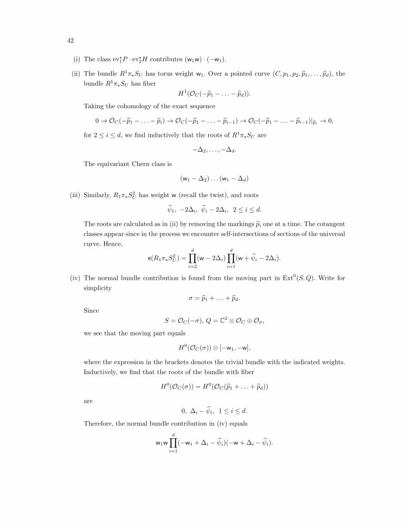
(i) The class ev?1P · ev?2H contributes (w1w) · (−w1).

(ii) The bundle R1π?SU has torus weight w1. Over a pointed curve (C, p1, p2, p1, . . . , pd), the

bundle R1π?SU has fiber

H1(OC(−p1 − . . .− pd)).

Taking the cohomology of the exact sequence

0→ OC(−p1 − . . .− pi)→ OC(−p1 − . . .− pi−1)→ OC(−p1 − . . .− pi−1)|pi → 0,

for 2 ≤ i ≤ d, we find inductively that the roots of R1π?SU are

−∆2, . . . ,−∆d.

The equivariant Chern class is

(w1 −∆2) . . . (w1 −∆d)

(iii) Similarly, R1π?S2U has weight w (recall the twist), and roots

ψ1, −2∆i, ψi − 2∆i, 2 ≤ i ≤ d.

The roots are calculated as in (ii) by removing the markings pi one at a time. The cotangent

classes appear since in the process we encounter self-intersections of sections of the universal

curve. Hence,

e(R1π?S2U ) =

d∏i=2

(w − 2∆i)

d∏i=1

(w + ψi − 2∆i).

(iv) The normal bundle contribution is found from the moving part in Ext0(S,Q). Write for

simplicity

σ = p1 + . . .+ pd.

Since

S = OC(−σ), Q = C2 ⊗OC ⊕Oσ,

we see that the moving part equals

H0(OC(σ))⊗ [−w1,−w],

where the expression in the brackets denotes the trivial bundle with the indicated weights.

Inductively, we find that the roots of the bundle with fiber

H0(OC(σ)) = H0(OC(p1 + . . .+ pd))

are

0, ∆i − ψi, 1 ≤ i ≤ d.

Therefore, the normal bundle contribution in (iv) equals

w1wd∏i=1

(−w1 + ∆i − ψi)(−w + ∆i − ψi).

3.1. Local geometries 43

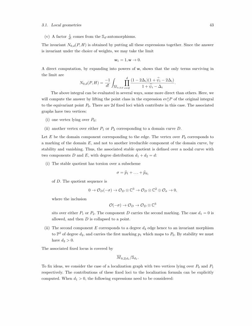
(v) A factor 1d! comes from the Sd-automorphisms.

The invariant N0,d(P,H) is obtained by putting all these expressions together. Since the answer

is invariant under the choice of weights, we may take the limit

w1 = 1,w→ 0.

A direct computation, by expanding into powers of w, shows that the only terms surviving in

the limit are

N0,d(P,H) =−1

d!

∫M0,2|d

d∏i=2

(1− 2∆i)(1 + ψi − 2∆i)

1 + ψi −∆i

.

The above integral can be evaluated in several ways, some more direct than others. Here, we

will compute the answer by lifting the point class in the expression ev?1P of the original integral

to the equivariant point P0. There are 2d fixed loci which contribute in this case. The associated

graphs have two vertices:

(i) one vertex lying over P0;

(ii) another vertex over either P1 or P2 corresponding to a domain curve D.

Let E be the domain component corresponding to the edge. The vertex over P0 corresponds to

a marking of the domain E, and not to another irreducible component of the domain curve, by

stability and vanishing. Thus, the associated stable quotient is defined over a nodal curve with

two components D and E, with degree distribution d1 + d2 = d:

(i) The stable quotient has torsion over a subscheme

σ = p1 + . . .+ pd1

of D. The quotient sequence is

0→ OD(−σ)→ OD ⊗ C3 → OD ⊗ C2 ⊕Oσ → 0,

where the inclusion

O(−σ)→ OD → OD ⊗ C3

sits over either P1 or P2. The component D carries the second marking. The case d1 = 0 is

allowed, and then D is collapsed to a point.

(ii) The second component E corresponds to a degree d2 edge hence to an invariant morphism

to P2 of degree d2, and carries the first marking p1 which maps to P0. By stability we must

have d2 > 0.

The associated fixed locus is covered by

M0,2|d1/Sd1

.

To fix ideas, we consider the case of a localization graph with two vertices lying over P0 and P1

respectively. The contributions of these fixed loci to the localization formula can be explicitly

computed. When d1 > 0, the following expressions need to be considered:

44

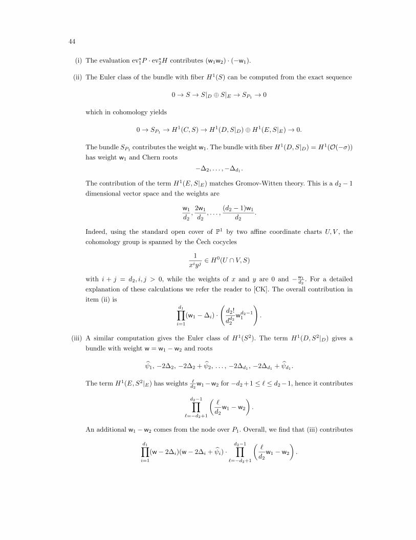
(i) The evaluation ev?1P · ev?2H contributes (w1w2) · (−w1).

(ii) The Euler class of the bundle with fiber H1(S) can be computed from the exact sequence

0→ S → S|D ⊕ S|E → SP1 → 0

which in cohomology yields

0→ SP1 → H1(C, S)→ H1(D,S|D)⊕H1(E,S|E)→ 0.

The bundle SP1contributes the weight w1. The bundle with fiberH1(D,S|D) = H1(O(−σ))

has weight w1 and Chern roots

−∆2, . . . ,−∆d1 .

The contribution of the term H1(E,S|E) matches Gromov-Witten theory. This is a d2 − 1

dimensional vector space and the weights are

w1

d2,

2w1

d2, . . . ,

(d2 − 1)w1

d2.

Indeed, using the standard open cover of P1 by two affine coordinate charts U, V , the

cohomology group is spanned by the Cech cocycles

1

xiyj∈ H0(U ∩ V, S)

with i + j = d2, i, j > 0, while the weights of x and y are 0 and −w1

d2. For a detailed

explanation of these calculations we refer the reader to [CK]. The overall contribution in

item (ii) isd1∏i=1

(w1 −∆i) ·

(d2!

dd22

wd2−11

).

(iii) A similar computation gives the Euler class of H1(S2). The term H1(D,S2|D) gives a

bundle with weight w = w1 − w2 and roots

ψ1, −2∆2, −2∆2 + ψ2, . . . , −2∆d1, −2∆d1

+ ψd1.

The term H1(E,S2|E) has weights `d2w1−w2 for −d2 +1 ≤ ` ≤ d2−1, hence it contributes

d2−1∏`=−d2+1

(`

d2w1 − w2

).

An additional w1 −w2 comes from the node over P1. Overall, we find that (iii) contributes

d1∏i=1

(w − 2∆i)(w − 2∆i + ψi) ·d2−1∏

`=−d2+1

(`

d2w1 − w2

).

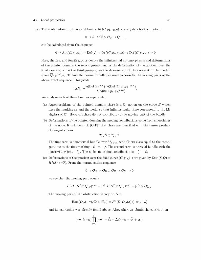
3.1. Local geometries 45

(iv) The contribution of the normal bundle to (C, p1, p2, q) where q denotes the quotient

0→ S → C3 ⊗OC → Q→ 0

can be calculated from the sequence

0→ Aut(C, p1, p2)→ Def (q)→ Def (C, p1, p2, q)→ Def (C, p1, p2)→ 0.

Here, the first and fourth groups denote the infinitesimal automorphisms and deformations

of the pointed domain, the second group denotes the deformation of the quotient over the

fixed domain, while the third group gives the deformation of the quotient in the moduli

space Q0,2(P2, d). To find the normal bundle, we need to consider the moving parts of the

above exact sequence. This yields

e(N) =e(Def (q)mov) · e(Def (C, p1, p2)mov)

e(Aut(C, p1, p2)mov).

We analyze each of these bundles separately.

(a) Automorphisms of the pointed domain: there is a C? action on the curve E which

fixes the marking p1 and the node, so that infinitesimally these correspond to the Lie

algebra of C?. However, these do not contribute to the moving part of the bundle.

(b) Deformations of the pointed domain: the moving contributions come from smoothings

of the node. It is known (cf. [GrP]) that these are identified with the tensor product

of tangent spaces

TP1D ⊗ TP1

E.

The first term is a nontrivial bundle over M0,2|d1with Chern class equal to the cotan-

gent line at the first marking −ψ1 = −ψ. The second term is a trivial bundle with the

nontrivial weight −w1

d2. The node smoothing contribution is −w1

d2− ψ.

(c) Deformations of the quotient over the fixed curve (C, p1, p2) are given by Ext0(S,Q) =

H0(S∨ ⊗Q). From the normalization sequence

0→ OC → OD ⊕OE → OP1→ 0

we see that the moving part equals

H0(D,S∨ ⊗Q|D)mov +H0(E,S∨ ⊗Q|E)mov − (S∨ ⊗Q)P1.

The moving part of the obstruction theory on D is

Hom(OD(−σ),C2 ⊗OD) = H0(D,OD(σ))[−w1,−w]

and its expression was already found above. Altogether, we obtain the contribution

(−w1)(−w)

d1∏i=1

(−w1 − ψi + ∆i)(−w − ψi + ∆i).

46

Over the curve E, the quotient comes from a degree d2 map f : E → P2, so that

S∨ ⊗Q|E = f?TP2.

We need to calculate

H0(E, f?TP2)mov − (f?TP2)P1.

Such expressions are well-known from Gromov-Witten theory, but for completeness

let us go through their derivation briefly. We make use of the Euler sequence

0→ O → C3 ⊗O(1)→ TP2 → 0.

Then, the expression to calculate becomes

(H0(f?O(1))⊗ C3)mov − (f?TP2)P1.

The weights on H0(f?O(1)) are

−`w1

d2, 0 ≤ ` ≤ d2,

while the weights on C3 are 0,w1,w2. We find that the total contribution from E is

−

(d2!2

d2d22

w2d21

)·d2∏`=0

(`

d2w1 − w2

)× 1

(−w1) · (−w).

Altogether, the contribution of (iv) becomes:

e(N) =

(w1

d2+ ψ

)·d1∏i=1

(−w1 − ψi + ∆i)(−w − ψi + ∆i)

(d2!2

d2d22

w2d21

)·d2∏`=0

(`

d2w1 − w2

).

(v) The factor 1d1!d2

accounts for automorphisms.

We collect all the terms (i)-(v) together. In the limit

w→ 0, w1 = 1

the only terms surviving are

(−1)d2

2d1!

(2d2

d2

)∫M0,2|d1

d1∏i=2

(1− 2∆i)(1− 2∆i + ψi)

1−∆i + ψi

=(−1)d2+1

2

(2d2

d2

)N0,d1

(P,H).

The case of the vertex lying over P2 is identical.

The formulas for the normal bundle are slightly different for the two fixed loci with d1 =

0, d2 = d. Redoing the above computation, we obtain that the combined contribution of the fixed

loci is

(−1)d−1 dd−1

d!

[w2

w1 − w2

d−1∏`=1

(`

d+

w2

w1

)+

w1

w2 − w1

d−1∏`=1

(`

d+

w1

w2

)].

3.1. Local geometries 47

In the limit w→ 0, w1 = 1, the above expression equals

(−1)d(

2d

d

)( d∑`=1

1

d+ `

).

Putting everything together, we obtain that

N0,d(P,H) =∑

d1+d2=d

d1>0, d2>0

(−1)d2+1

(2d2

d2

)N0,d1(P,H) + (−1)d

(2d

d

)( d∑`=1

1

d+ `

).

The following Lemma shows inductively that

N0,d(P,H) =(−1)d

2d

(2d

d

).

Lemma 1. For all d > 0, we have

∑d1+d2=d

d1>0,d2≥0

1

2d1

(2d1

d1

)(2d2

d2

)=

(2d

d

)( d∑`=1

1

d+ `

).

Proof. Since (2d

d

)= (−4)d

(− 1

2

d

)it suffices to show that

∑d1+d2=d

d1>0,d2≥0

1

2d1

(− 1

2

d1

)(− 1

2

d2

)=

(− 1

2

d

)( d∑`=1

1

d+ `

).

We consider three generating functions

f(z) =

∞∑d=0

(− 1

2

d

)zd, g(z) =

∞∑d=1

1

2d

(− 1

2

d

)zd

and finally

h(z) =

∞∑d=1

(− 1

2

d

)( d∑`=1

1

d+ `

)zd.

We claim that

h(z) = f(z)g(z),

thus establishing the lemma by matching the coefficient of zd on both sides. From the binomial

theorem, we compute

f(z) =1√

1 + z.

The series g(z) is obtained by integrating f(z)−12z hence

g(z) =

∫1

2z

(1√

1 + z− 1

)dz = − ln

(√1 + z + 1

2

).

48

The calculation of h(z) is slightly more involved. We note

h(z) =∑d

(− 1

2

d

)( d∑`=1

∫ 1

0

td+`−1 dt

)zd

=∑d

(− 1

2

d

)(∫ 1

0

td − t2d

1− tdt

)zd

=

∫ 1

0

(1 + zt)−12 − (1 + zt2)−

12

1− tdt

= − 1√1 + z

ln

(1 + zt+

√(1 + z)(1 + zt2)

(√

1 + z +√

1 + zt)2

)t=1

t=0

= − 1√1 + z

ln

(√1 + z + 1

2

)= f(z)g(z).

This completes the proof of Proposition 3 in genus 0. We leave the simpler genus 1 calculation

to the reader.

Exercise 17. Calculate the genus 0 and genus 1 primary invariants of the local 5-fold

O(−1)⊕O(−1)⊕O(−1)→ P2.

The answer in Gromov-Witten theory is given in [PZ], Lemma 3.1.

Exercise 18. (cf. [T]) Show that the genus 1 degree 1 stable quotient invariant of the local geometry

OP2(−3)→ P2 equals ∫Q1,0(P2,1)

e(H1(S3)) =3

4,

using the description of the moduli space Q1,0(P2, 1) = M1,1 × P2. The answer differs from

Gromov-Witten theory.

Example 13. For the Calabi-Yau local geometry

X = O(−a1)⊕ . . .⊕O(−ak)→ Pn, a1 + . . .+ ak = n+ 1, ai > 0,

the obstruction bundle

V → Q0,2(Pn, d)

has fiber

H1(Sa1)⊕ . . .⊕H1(Sak).

The local invariants of X are constructed via the Euler class of V. The case of 1-point genus 0

invariants was considered by Cooper and Zinger. The resulting formulas, as stated in [CZ], take

the explicit form (over the two pointed moduli space):∫Q0,2(Pn,d)

e(V) · ψn−1−i1 · ev?1H

k+i = (−1)d(n+1)+k coefficient of xn−k−i in I(x)

for all 0 ≤ i ≤ n− k, where

I(x) =

∏kj=1(ajx+ 1) · · · (ajx+ (ajd− 1))

(x+ 1)n+1 · · · (x+ d)n+1.

3.2. Hypersurface geometries 49

3.2 Hypersurface geometries

Let X ⊂ Pn be a projective variety. The stack of stable quotients to X

Qg,m(X, d) ⊂ Qg,m(Pn, d)

can be defined as the stack of quotients to Pn vanishing on X. Precisely, given a stable quotient

to Pn,

(C, p1, . . . , pm, 0→ S → Cn+1 ⊗OCq→ Q→ 0),

we obtain by dualizing n+ 1 sections s0, . . . , sn of S∨

Cn+1 ⊗OC → S∨.

We require that for every homogeneous degree k equation F of X, we have

F (s0, . . . , sn) = 0 ∈ H0(C, S−k).

The resulting moduli space Qg,m(X, d) thus depends on the projective embedding of X.

Example 14. Consider the moduli space Q1,0(Xn+1 ⊂ Pn, d) of stable quotients associated to the

Calabi-Yau hypersurface of degree n+ 1:

Xn+1 ⊂ Pn.

We remarked already in Example 10 that Q1,0(Pn, d) is nonsingular of expected dimension (n+

1)d. As before, let SU be the universal subsheaf on the universal curve

π : U → Q1,0(Pn, d).

The pushforward sheaf

π∗

(S−(n+1)U

)→ Q1,0(Pn, d)

is locally free of rank (n + 1)d, and the higher cohomology vanishes. This is clear over smooth

genus 1 domains, while the case of necklaces of rational curves has to be treated separately. The

defining equation

F = 0

of Xn+1 ⊂ Pn yields a canonical section of the bundle

π∗

(S−(n+1)U

)→ Q1,0(Pn, d)

given by

(C, 0→ S → Cn+1 ⊗OC → Q→ 0) 7→ F (s0, . . . , sn).

The section cuts out the moduli space of quotients to the hypersurface Xn+1. Thus, genus 1

stable quotient invariants of Xn+1 ⊂ Pn can be defined by the integral

〈〉Xn+1

1,d =

∫Q1,0(Pn,d)

e(π∗

(S−(n+1)U

)). (3.9)

50

Thus, elliptic stable quotient invariants are given by construction by the Euler class of a tauto-

logical bundle. In Gromov-Witten theory, substantial work is required to express the invariants

in this form, see [Z1].

Exercise 19. Evaluate the degree 2 stable quotients of the smooth plane cubic∫Q1,0(P2,2)

e(H0(S−3))

by equivariant localization. With an appropriate choice of weights, there are only 6 fixed loci to

consider.

Remark 10. If X ⊂ Pn is nonsingular complete intersection, the moduli space of quotients to X

admits a virtual fundamental class in all genera. This will follow on general grounds from the

discussion of GIT geometries in the last section, but it can also be seen directly, cf. [MOP].

Example 15. In Gromov-Witten theory, the J-function of Pn encodes 1-point genus 0 descendant

invariants. Specifically, we set

JPn(q, h) =∑d

qd(ev1)?

([M0,1(Pn, d)]

h(h− ψ1)

)∈ H?(Pn)[[q, h−1]].

The relevance of the J-function to Gromov-Witten theory comes from at least two sources:

(i) for varieties whose cohomology is generated by divisor classes, such as Pn, all descendant

genus zero multiple point invariants can be reconstructed from the descendant genus zero

1-point invariants [LP], [BK];

(ii) a second motivation is given by quantum cohomology and quantum differential equations:

the differential equations that J satisfies yield relations in quantum cohomology.

Fortunately, it is not very hard to calculate the J function explicitly, via the localization theorem

applied to a space of graphs of stable maps [Gi]. The answer takes the form

JPn(q, h) =∑d

qd · 1

(H + h)n+1(H + 2h)n+1 · · · (H + dh)n+1.

Consider now a degree ` complete intersection X ⊂ Pn. The calculation of the J-function is

feasible in this case as well. First, to describe the moduli space of maps to X, consider the rank

d`+ 1 bundle

V` = π?(ev?O(`))→M0,1(Pn, d),

where π and ev denote the projection from the universal curve overM0,1(Pn, d) and the evaluation

morphism. The defining equation F = 0 of X yields a section of the bundle

V` →M0,1(Pn, d)

cutting out the moduli space of maps to X. This shows that

i?[M0,1(X, d)]vir = e(V`) ∩ [M0,1(Pn, d)].

3.2. Hypersurface geometries 51

We define the cohomology valued function

JMX (q, h) =

∑d

qd(ev1)?

([M0,1(X, d)]vir

h(h− ψ1)

)∈ H?(Pn)[[q, h−1]].

In the above, we are using the evaluation map to the target Pn, not to the complete intersection

X. If γi is a basis for the cohomology of Pn, and γi is the dual basis, then

JMX (q, h) =

∑d

∞∑k=0

qdh−k−2

(∫[M0,1(X,d)]vir

ψk1 ev?1 γi

)· γi.

This expression does not generalize to stable quotients since the moduli space of quotients

is undefined when (g,m) = (0, 1). We need to have at least 2 markings for the quotient stability

condition to be meaningful. Fortunately, we may express the J-function via the moduli spaces of

maps with two markings. Indeed, by the string equation in Gromov-Witten theory, we have

JMX (q, h) =

∑d

∞∑k=−1

qdh−k−2

(∫M0,2(Pn,d)

e(V`) · ψk+11 ev?1γ

i

)· γi

which can be rewritten in the compact form

JMX (q, h) =

∑d

qd(ev1)?

(e(V`) ∩ [M0,2(Pn, d)]

h− ψ1

).

To write down the explicit expression of the J-function of X, first define the cohomology

valued I-function

IX(q, h) =∑d

qd · (`H)(`H + h)(`H + 2h) · · · (`H + `d · h)

(H + h)n+1(H + 2h)n+1 · · · (H + dh)n+1∈ H?(Pn)[[q, h−1]].

The quantum Lefschetz hyperplane section theorem [Gi] connects the functions I and J :

(i) when ` ≤ n− 1, i.e. for Fano hypersurfaces of index at least 2, we have

JMX (q, h) = IX(q, h);

(ii) when ` = n, i.e. for Fano hypersurfaces of index 1, we have

JMX (q, h) = exp

(−`!qh

)IX(q, h);

(iii) when ` = n + 1, i.e. in the Calabi-Yau case, the relationship between J and I involves a

mirror change of coordinates, which determines the invariants recursively.

Example 16. Similarly, we can define the J-function for stable quotient invariants of a hypersur-

face X of degree ` in terms of the Euler class of the tautological pushforward bundle

VQ` = π?(S

−`U )→ Q0,2(Pn, d).

52

We then define the stable quotient analogue of the J-function as the cohomology valued function

JQX(h, q) = 1 +

∑d6=0

qd(ev1)?

(e(VQ

` ) ∩ [Q0,2(Pn, d)]

h− ψ1

)∈ H?(Pn)[[q, h−1]].

The quantum hyperplane theorem for stable quotients was established by Cooper and Zinger:

Theorem 9. [CZ]

(i) In the Fano case ` ≤ n, we have

JQX(q, h) = IX(q, h).

(ii) In the Calabi-Yau case ` = n+ 1, we have

JQX(q, h) =

IX(q, h)

h(q)

where

h(q) =

∞∑d=0

qd(d(n+ 1))!

(d!)n+1.

Hence, in the Fano case, the stable quotient invariants take almost the same form as for

stable maps. In fact, the formulas are exactly matched for Fano geometries of index at least

2. The J function is simpler for quotients than for maps to Calabi-Yau hypersurfaces, and it

is more directly related to the I-function. Rephrasing, it is the stable map and stable quotient

J-functions of Calabi-Yau hypersufaces that differ by a mirror transform. The simpler form of

the answer suggests that stable quotients may be the curve counting theory most directly related

to the B-side of mirror symmetry.

The method of proof of Theorem 9 follows the roadmap provided by Givental’s calculation

in Gromov-Witten theory [Gi]. We refer the reader to [CK] or [HKKPTVZZ] for an overview of

the method. While the precise details of the argument are beyond the scope of this presentation,

the main points are:

(i) first, one establishes a stronger equality involving the equivariant versions of I and J ;

(ii) the equivariant correspondence is proven first for Fano geometries of index at least 2. To

this end, [CZ] relies on a uniqueness result for power series which was also used in Gromov-

Witten theory. The central notions studied here are C-recursivity and self-polynomiality.

Without introducing the relevant definitions, we only mention that both I and J satisfy

these properties. For I, this can be checked directly from the explicit expression. For J , the

two properties are consequences of the localization theorem applied to suitable integrals on

the moduli space of stable quotients. Since the low order terms in I and J agree for Fanos

of index at least 2, the match between I and J is achieved in this case.

4.0. Variation of stability 53

(iii) The main difference between stable quotients and stable maps becomes manifest for Calabi-

Yau geometries. Relating I and J is a consequence of a recursion involving twisted Hodge

integrals on certain moduli spaces of weighted pointed stable curves. Surprisingly, the re-

cursion needed in the Calabi-Yau case is identical to the one arising in Fano geometries. In

some sense, the Fano geometries determine the Calabi-Yau answer as well.

Finally, the formulas of [CZ] apply more generally to the J-function of complete intersections

in projective space and products of projective spaces. The two point and three point J-functions

are moreover discussed in [Z2]. The next section will present results which cover even more general

situations.

Section 4: Wall-crossing and other geometries

4.0 Variation of stability

In this subsection, we introduce a variant of stable quotients which depends on a positive pa-

rameter ε > 0. The idea of ε-stable quotients originates from Hassett’s weighted pointed curves

reviewed in Section 2, and the work of Mustata-Mustata [MM] in rank 1. In arbitrary rank, ε-

stable quotients were introduced by Toda in [T], who studied the resulting wall-crossing formulas

as the stability parameter varies. We give an account of Toda’s results.

To begin, fix a rational parameter ε > 0. Then,

Definition 5. [T] An ε-stable quotient (C, p1, . . . , pm, q) consists in

(i) a connected, projective, reduced, nodal curve (C, p1, . . . , pm) with m markings;

(ii) the markings are smooth disjoint points of the domain;

(iii) a short exact sequence over C,

0→ S → Cn ⊗OC → Q→ 0

where S has rank r and degree −d, such that

(iv) Q is locally free at the nodes and markings, and furthermore, for any p ∈ C, the torsion Tsheaf of Q satisfies

lengthp(T ) ≤ 1

ε;

(v) the line bundle

ωC(p1 + . . .+ pm)⊗ (ΛrS∨)ε

is ample.

Note that ampleness is only required for a fixed value of ε in condition (v).

Similarly to usual stable quotients, we can construct a moduli space of ε-stable quotients:

54

Theorem 10. [T] There exists a separated proper Deligne-Mumford stack of ε-stable quotients

Qε

g,m(G(r, n), d)

which admits a two-term perfect obstruction theory and a virtual fundamental class.

Exercise 20. (cf. [T]) Let C ∼= P1 ⊂ Pn be a line, and let p, q ∈ C be two distinct points.

Multiplication by the n+ 1 linear terms x0, . . . , xn yields an injective map

0→ OC(−1)→ Cn+1 ⊗OC .

Consider furthermore a natural inclusion

0→ OC(−p− q − 1)→ Cn+1 ⊗OC

with quotient Q. Show that the above quotient is stable for ε = 1, but does not come from a stable

quotient or a stable map.

Example 17. To understand how the moduli spaces change as stability varies, we may consider

two different cases. First, when

ε ≤ 1

d,

condition (iv) about the length of the torsion sheaf is vacuous. Similarly, by the interpretation of

stability in terms of the number of markings on rational components, it follows that any stable

quotient is automatically ε-stable and conversely. Therefore,

Qε

g,m(G(r, n), d) = Qg,m(G(r, n), d), for ε ≤ 1

d.

Similarly, when ε > 2, condition (iv) simply says that Q is locally free, hence it must come from

a map

f : C → G(r, n).

Condition (v) means that each collapsed component must have least 3 markings or nodes. Hence

Qε

g,m(G(r, n), d) = Mg,m(G(r, n), d), for ε > 2.

The following result explains how the different moduli spaces of ε-stable quotients interpolate

between stable quotients and stable maps:

Proposition 4. [T] There are finitely many values

0 = ε0 < ε1 < . . . < εk < εk+1 =∞

such that for all ε ∈ (εi−1, εi] we have

Qε

g,m(G(r, n), d) = Qεig,m(G(r, n), d).

4.0. Variation of stability 55

Exercise 21. (cf. [T]) Prove the above Proposition. In fact, show that when (g,m) 6= (0, 0), we

may take

εi =1

d− i+ 1, 1 ≤ i ≤ d.

The case (g,m) = (0, 0) needs to be considered separately.

Furthermore, in rank r = 1, the natural contraction morphism

c : Mg,m(G(1, n), d)→ Qg,m(G(1, n), d)

can be factored as composition of contraction maps

cε,ε′ : Qε

g,m(G(1, n), d)→ Qε′

g,m(G(1, n), d),

for 0 < ε′ < ε in such a fashion that

(cε,ε′)?[Qε

g,m(G(1, n), d)]vir = [Qε′

g,m(G(1, n), d)]vir.

As a consequence, the stable quotient invariants are also matched:

Theorem 11. [T] The ε-stable quotient invariants of G(1, n) are independent of the choice of

parameter ε > 0. The same result holds for G(r, n), using the Plucker embedding.

Example 18. To understand the contraction morphisms cε,ε′ consider the case (g,m) 6= (0, 0), (1, 0)

and a wall-crossing corresponding to successive stability parameters

εi+1 =1

d− i, εi =

1

d− i+ 1, 1 ≤ i ≤ d− 1.

By requirements (iv) and (v) of the definition, all εi+1-stable quotients satisfy

(i) the torsion sheaf of Q must have length less or equal to d− i at each point p ∈ C,

(ii) each genus 0 component P must have either:

– at least 3 special points (markings or nodes), or else

– 2 special points, and the degree of S∨ over P must be positive, or else

– 1 special point, and the degree of S∨ over P must be bigger or equal than d− i+ 1.

These quotients are automatically εi-stable, unless S∨ has degree exactly d− i+ 1 on a genus 0

component P containing exactly one special point. Under the contraction morphism

ci : Qεi+1

g,m (G(1, n), d)→ Qεig,m(G(1, n), d),

such a component must then be collapsed to a point over which the quotient Q acquires torsion

of length d− i+ 1.

Finally, we can explicitly describe the ε-stable quotients to the point G(1, 1). We leave this

description as an exercise:

56

Exercise 22. (cf. [T])

(i) Consider the following collection of m+d weights, with m weights equal to 1, and d weights

equal ε:

a = (1, . . . , 1, ε, . . . , ε).

Show that the moduli space of ε-stable quotients is related to the Hassett moduli space of

a-stable curves as follows

Mg,a/Sd → Qε

g,m(G(1, 1), d).

(ii) In particular, when (g,m) = 0, when d = 2d′ + 1 ≥ 3 is odd, show that for ε = 1d′ , we have

Qε

0,0(G(1, 1), d) ∼= Pd//SL2.

Thus, all other nonempty moduli spaces Qε

0,0(G(1, 1), d) are obtained as sequences of weighted

blowups of Pd//SL2. What happens for d even?

4.1 Quasimaps to GIT quotients

In this subsection, we will greatly enlarge the class of targets for which stable quotient invariants

may be defined by including quite general examples of GIT quotients. The correct definition is

due to Ciocan-Fontanine, Kim and Maulik in [CFKM], whose presentation we follow; see also

[CFKi1] for the important special case of toric varieties.

To begin, consider the linear action of a reductive algebraic group G on an affine variety

W → V ∼= An.

We fix a character θ of G, defining a G-equivariant line bundle over W :

Lθ = W × Cθ →W.

In this setup, we can form three different quotients

(i) the affine quotient

W/aff G = Spec(A(W )G);

(ii) the GIT quotient

W//θG = Proj

⊕m≥0

H0(W,Lmθ )G

;

(iii) the stack quotient [W/G].

The inclusion

A(W )G →⊕m

H0(W,Lmθ )G

4.1. Quasimaps to GIT quotients 57

yields a natural projective morphism

W//θG→W/aff G,

with Lθ giving a relative polarization. When the affine quotient is a point, the GIT quotient

W//θG is projective.

We furthermore make the following two assumptions on the set of stable points of W :

(i) W s = W ss 6= ∅ is smooth;

(ii) G acts freely on W s.

As a consequence, we obtain

W//θG = [W s/G] → [W/G].

Example 19. The following examples are pertinent to the above setup, cf. [CFKM]:

(i) Let W = V = Hom(Cr,Cn) and G = GLr, with character given by θ = det. In this case,

we have

W//θG = G(r, n), W/aff G = pt.

More generally, we consider

1 ≤ k1 < k2 < . . . < k`+1 = n

a collection of integers, and let the group

G = GLk1× . . .×GLk`

act on the vector space

W = V = Hom(Ck1 ,Ck2)⊕ . . .⊕Hom(Ck` ,Ck`+1)

via

(g1, . . . , g`)(A1, . . . , A`) = (g−12 A1 g1, . . . , A` g`).

The quotient is the partial flag variety

W//θG = F(k1, . . . , k`, n)

parametrizing flags

W1 ⊂W2 ⊂ . . . ⊂W` ⊂ Cn, dimWi = ki.

(ii) Let W = V = Cn, G = Tr. In this case we get toric varieties. Concretely, consider dual

lattices N = M∨, and a complete nonsingular fan

Σ ⊂ N ⊗ R

58

generated by a set of one dimensional integral rays Σ(1). There is a natural surjection

(C?)Σ(1) → C? ⊗N

whose kernel is denoted by G. The group G → (C?)Σ(1) then acts on CΣ(1), and the unstable

points are

Z(Σ) = (zρ)ρ∈Σ(1) :∏ρ6⊂σ

zρ = 0 for all maximal dimensional faces σ of Σ.

Then,

W s = CΣ(1) \ Z(Σ),

and the quotient is the toric variety associated to Σ,

W//θG = XΣ.

We note for further use that the equations zρ = 0 in CΣ(1) cut out divisors Dρ in XΣ,

for ρ ∈ Σ(1). These divisors are easily seen to be subject to the following relations in the

Picard group of XΣ: ∑ρ

〈ρ,m〉Dρ = 0 for all m ∈M.

(iii) If X ⊂ Pn−1 is a complete intersection, then we may take W = CX, the cone of X in affine

Cn, and let G = C? act on Cn with the usual weights. Then

X = W//θG.

(iv) (cf. [CFKi2]) Let (W,G, θ) be a GIT datum as above, with W smooth. Consider E a finite

dimensional representation of G, giving rise to a bundle

E = W s ×G E →W//θG.

A global G-invariant section s of the trivial bundle W ×E →W then descends to a section

s of the bundle E →W//θG. Assume that s is regular, and that its zero locus X = Zero(s)

is smooth of the expected dimension. Then, X can be represented as a quotient

X = Zero(s)//θG

satisfying the above requirements.

In the context of (ii), smooth complete intersections in toric varieties can be generated in

this fashion. Flag manifolds of type B,C,D are also obtained this way via (i), by taking

W//θG to be a flag manifold of type A.

(v) Examples (i)-(iv) are not the only ones. For instance, local targets

E ×GW →W//θG

over projective GIT quotients W//θG can be considered, at least when W × E → W has

no G-invariant holomorphic sections.

4.1. Quasimaps to GIT quotients 59

To arrive at the definition of a stable quotient, or a stable quasimap in the language of

[CFKM], we start with the observation that any morphism

f : (C, p1, . . . , pm)→W//θG

naturally yields a morphism to the stack quotient

f : C → [W/G].

As such, f determines a principal G-bundle P → C together with a G-equivariant morphism

f : P →W.

Such an equivariant morphism f induces a section

sf : C → P ×GW

of the fiber bundle

P ×GW → C.

Finally, the character θ induces a bundle

Lθ → P×GW

which yields by pullback a line bundle

s?fLθ ∼= P ×G Cθ → C.

Motivated by these considerations, we have the following:

Definition 6. [CFKM] A stable quasimap to W//θG consists in

(i) a connected, projective, reduced, nodal curve (C, p1, . . . , pm) of arithmetic genus g, with

distinct markings which are smooth points of the domain;

(ii) a principal G-bundle P → C, and a section s of the fiber bundle P ×GW → C such that:

(iii) there are finitely many basepoints y ∈ C, that is points that map to the unstable locus of

W :

s(y) ∈ Py ×G (W \W s) ∼= W \W s.

The basepoints are neither nodes nor markings;

(iv) the line bundle

ωC(p1 + . . .+ pm)⊗ s?Lεθ

is ample for all ε > 0 rational.

The following theorem extends some of the main results about stable quotients to stable

quasimaps.

60

Theorem 12. [CFKM]

(i) There is a separated Deligne Mumford stack parametrizing stable quasimaps of fixed degree,

endowed with a natural proper morphism to the affine quotient W/aff G.

(ii) The moduli space of quasimaps has a two-term perfect obstruction theory when W has at

worst lci singularities.

In particular, pertinent to example (iii), when X is a complete intersection in Pn, there is

a well-defined virtual fundamental class for the moduli space of stable quotients to X. Other

examples include

- smooth toric varieties, smooth complete intersections in toric varieties, flag varieties of type

A,B,C,D, quiver varieties, and others.

As a result, we can define quasimap invariants for the targets for which Theorem 12 applies. We

will denote the corresponding invariants as

〈τa1γ1, . . . , τamγm〉Qg,m,β =

∫[Qg,m(W//θ G,β)]vir

m∏i=1

ψaii · ev?i γi.

The integrals are well-defined when the target W//θG is projective so that the moduli spaces

are proper. The resulting invariants do depend on the pair of stacks [W/G] and [W s/G]. This is

weaker than claiming invariance on the GIT quotient alone.

Remark 11. We can extend the above definition to quasiprojective targets X = W//θG endowed

with an action of a torus T, i.e. an action of T on W commuting with the action of G. In addition

to the hypotheses of Theorem 12, we assume that

(i) the action of T on the affine quotient W/aff G has proper fixed sets.

This is satisfied for many examples of interest.

Assumption (i) implies that the torus fixed loci of the moduli space of quasimaps are proper.

The quasimap invariants are then defined by formally applying the virtual localization theorem

of Graber and Pandharipande [GrP], via a sum of integrals over the fixed loci. The answer may

depend on the torus weights. As a result, the quasimap invariants take values in the localized

equivariant cohomology of the point.

Example 20. Following [CFKi1], let us spell out the details of the definition of quasimaps to the

projective smooth toric variety XΣ associated to a complete nonsingular fan

Σ ⊂ N ⊗ R,

where N = M∨ is the dual of a lattice M . We fix a polarization OXΣ(1) = ⊗ρO(Dρ)

αρ , for

integers αρ, where Dρ is the divisor in XΣ corresponding to the ray ρ ∈ Σ(1).

In this case, we parametrize

4.2. Quasimap invariants of semi-positive GIT targets 61

(i) connected, projective, reduced, nodal curves (C, p1, . . . , pm) of arithmetic genus g with

distinct m smooth markings,

(ii) line bundles of fixed degrees dρ together with sections (Lρ, uρ) over C, one for each ray ρ

of Σ(1),

(iii) a collection of trivializations

φm :⊗ρ

L〈ρ,m〉ρ → OC for m ∈M

compatible in the sense that

φm1⊗ φm2

= φm1+m2.

The data is required to satisfy a nondegeneracy condition

(iv) there are finitely many basepoints which are neither markings nor nodes,

and the typical quotient stability regarding the ampleness of the bundle

ωC(p1 + . . .+ pm)⊗

⊗ρ∈Σ(1)

Lαρρ

ε

for all rational ε > 0. By definition, a basepoint y ∈ C of the quasimap has the property that

for all maximal faces σ of Σ, there exists a ray ρ 6⊂ σ such that uρ(y) = 0.

The line bundles Lρ correspond to the divisors Dρ for ρ ∈ Σ(1), while the trivializations reflect

the relations in the Picard group∑ρ

〈ρ,m〉Dρ = 0 for all m ∈M.

Exercise 23. (cf. [CFKM]) How would you define ε-stable quasimaps to a projective GIT -quotient

W//θG as above, so that to ensure the existence of a proper moduli space with a two-term perfect

obstruction theory?

4.2 Quasimap invariants of semi-positive GIT targets

The last aspect of these notes concerns comparison between stable quotient and stable map

invariants for semipositive GIT quotients. We review here general conjectures and results recently

obtained by Ciocan-Fontanine and Kim, referring the reader to [CFKi1], [CFKi2], [CFKi3] for

more precise statements and proofs. These results provide vast generalizations of the calculations

discussed in the previous sections.

Throughout this subsection, we consider GIT quotients which permit the definition of

quasimap invariants via Theorem 12:

62

(i) W s = W ss 6= ∅ is smooth, G acts freely on W s, W has lci singularities.

Such quotients are allowed to be quasi-projective provided they satisfy the requirements of Re-

mark 11:

(ii) there is a torus action on W commuting with the action of G, such that the torus fixed

sets on W/aff G are proper.

As usual, whenever we use quasi-projective targets, the cohomology insertions are taken in the

torus-equivariant cohomology. We will make this convention throughout (and we will occasionally

reiterate it). Some readers may want to think about the projective quotients only for which (ii)

is not needed. Equivalently, the torus may be taken to be trivial in the projective case.

In addition, we will restrict to the following case from now on:

(iii) A triple (W,G, θ) yielding a quotient

X = W//θG

is semipositive provided that for all θ-effective classes β (i.e. classes which can be represented

by quasimaps to W//θG) we have

−β ·KW ≥ 0.

(In the projective case, these give quotients X = W//θG with nef anticanonical class.)

With these assumptions, we next introduce the relevant generating series of quasimap in-

variants. To this end, we fix (torus equivariant) cohomology classes tj ∈ H2?(X), and form the

formal power series

t(ψ) = t0 + t1ψ + t2ψ2 + . . . .

We define the descendat genus g quasimap potential of X to be

FQg (t) =

∑β,m

qβ

m!〈t(ψ1), . . . , t(ψm)〉Qg,m,β .

The sum is indexed by all pairs (β,m) for which stability is not vacuous, allowing for the definition

of the moduli space. The potential is defined over a suitable Novikov ring which for simplicity

we denote C[[q]] below, but we will be less precise regarding this aspect. Similarly, one can define

the genus g descendant Gromov-Witten potential

FMg (t) =

∑β,m

qβ

m!〈t(ψ1), . . . , t(ψm)〉Mg,m,β .

The main conjecture relating stable quasimap theory to Gromov-Witten theory then takes

the form:

4.2. Quasimap invariants of semi-positive GIT targets 63

Conjecture 1. [CFKi3] For any semipostive triple (W,G, θ) as above there exist power series

I0(q) ∈ C[[q]], I1(q) ∈ H2?(X)[[q]],

with I0 invertible, such that the quasimap and Gromov-Witten potentials are related by

FQg (t) = I0(q)2−2g · FM

g

(t + I1(q)

I0(q)

).

In fact, the conjecture in [CFKi3] applies to ε quasimap invariants, but we will not pursue

this level of generality here.

The power series I0(q) and I1(q) are explicit and are related to genus zero 2-point and

3-point quasimap invariants. To define them, we fix γi and γi two homogeneous dual bases for

the (localized torus equivariant) cohomology of X. We then define

I1(q)

I0(q)=∑i

γi∑β 6=0

〈γi, 1〉Q0,2,β · qβ

as a series in two point genus 0 quasimap invariants. Furthermore, I0 is built out of three point

genus 0 invariants1

I0(q)= 1 +

∑β 6=0

〈γi, γi, 1〉Q0,3,β · qβ .

It can be checked that the comparison results between stable map and stable quotient invariants

discussed for the geometries of Sections 2 and 3 are compatible with the transformation formula

of Conjecture 1.

Remark 12. (i) In the smooth projective Fano case, we have the simplification I0(q) = 1 for

dimension reasons, so the conjecture takes the form

FQg (t) = FM

g (t + I1(q)) .

(ii) For smooth projective Fano geometries of index two or higher, we obtain moreover I1(q) = 0,

so the conjecture becomes

FQg (t) = FM

g (t).

This would generalize the matching between stable quotient and Gromov-Witten invariants

explained throughout these notes in various contexts.

(iii) Finally, in the smooth quasi-projective toric case, we can find I0 and I1 explicitly. Indeed,

we read off I0 and I1 from the expansion of the small I-function

I(q, h) = I0(q) · 1 + I1(q) · 1

h+O

(1

h2

).

The expression for I is explicit. Using the notation of the previous subsection, I is the

hypergeometric series

I(q, h) = 1 +∑β 6=0

qβ∏

ρ∈Σ(1)

∏0j=−∞(c1(O(Dρ)) + jh)∏dρj=−∞(c1(O(Dρ)) + jh)

∈ H?(XΣ)[[q, h−1]].

64

(For quasi-projective targets, localized equivariant cohomology is used, for the action of

the torus T = (C?)Σ(1) on XΣ.) From here, one can see directly that for smooth projective

Fano toric varieties, we have

I0(q) = 1, I1(q) = 0;

see Chapter 11 of [CK] for details.

Conjecture 1 was established by Ciocan-Fontanine and Kim for several general geometries

of interest, cf. [CFKi3]:

Theorem 13. (i) In genus 0, the conjecture holds for semipositive quotients endowed with an

action of a torus with isolated fixed points;

(ii) in arbitrary genus, the conjecture holds for semipositive quasi-projective toric manifolds;

(iii) by considering twisted invariants, the conjecture is true in genus 0 for compact Calabi-Yau

complete intersections in toric or flag varieties. In arbitrary genus, Conjecture 1 holds for

the local CY geometry given by the total space of the canonical bundle of partial type A flag

varieties.

In particular, for smooth projective Fano toric varieties, (ii) confirms that the quasimap

and Gromov-Witten invariants agree in all genera

FQg (t) = FM

g (t) ,

as expected.

Bibliography

[Bea] A. Beauville, Sur la cohomologie de certains espaces de modules de fibres vectoriels, Ge-

ometry and Analysis, 37 – 40, Oxford University Press (1995).

[BF] K. Behrend, B. Fantechi, The intrinsic normal cone, Invent. Math. 128 (1997), 45 – 88.

[Ber] A. Bertram, Towards a Schubert calculus for maps from a Riemann surface to a Grass-

mannian, Internat. J. Math 5 (1994), 811 – 825.

[BDW] A. Bertram, G. Daskalopoulos and R. Wentworth, Gromov Invariants for holomorphic

maps from Riemann surfaces to Grassmannians, J. Amer. Math. Soc. 9 (1996), 529 – 571.

[BK] A. Bertram, H. Kley, New recursions for genus-zero Gromov-Witten invariants, Topology

44 (2005), 1 – 24.

[CFKa] I. Ciocan-Fontanine, M. Kapranov, Virtual fundamental classes via dg-manifolds, Geom.

Topol. 13 (2009), 1779 – 1804.

[CFKi1] I. Ciocan-Fontanine, B. Kim, Moduli stacks of stable toric quasimaps, Adv. Math. 225

(2010), 3022 – 3051.

[CFKi2] I. Ciocan-Fontanine, B. Kim, Wall-crossing in genus zero quasimap theory and mirror

maps, Algebr. Geom. 1 (2014), 400 – 448.

[CFKi3] I. Ciocan-Fontanine, B. Kim, Higher genus quasimap wallcrossings for semi-positive

targets, arXiv:1308:6377.

[CFKM] I. Ciocan-Fontanine, B. Kim, D. Maulik, Stable quasimaps to GIT quotients, J. Geom.

Phys. 75 (2014), 17 – 47.

[C] Y. Cooper, The geometry of stable quotients in genus 1, Math Ann. 361 (2015), 943 – 979.

[CZ] Y. Cooper, A. Zinger, Mirror symmetry for stable quotient invariants, Michigan Math. J.

63 (2014), 571 – 621.

[CK] D. Cox, S. Katz, Mirror symmetry and algebraic geometry, Mathematical Surveys and

Monographs 68, Amer. Math. Soc. 1999.

65

66 Bibliography

[ES] G. Ellingsrud, S. Stromme, Towards the Chow ring of the Hilbert scheme of P2, J. Reine

Angew. Math. 441 (1993), 33 – 44.

[G] D. Gillam, Deformations of quotients on a product, arXiv:1103.5482.

[Gi] A. Givental, Equivariant Gromov-Witten invariants, Inter. Math. Research Lett. 13 (1996),

613 – 663.

[GeP] E. Getzler, R. Pandharipande, The Betti numbers of M0,n(r, d), J. Algebraic Geom. 15

(2006), 709 – 732.

[GrP] T. Graber, R. Pandharipande, Localization of virtual classes, Invent. Math. 135 (1999),

487 – 518.

[H] B. Hassett, Moduli spaces of weighted pointed stable curves, Adv. Math. 173 (2003), 316 –

352.

[HM] J. Harris, I. Morrison, Moduli of curves, Springer-Verlag, New York, 1998.

[HKKPTVZZ] K. Hori, S. Katz, A. Klemm, R. Pandharipande, R. Thomas, C. Vafa, R. Vakil,

E. Zaslow, Mirror Symmetry, Clay Math. Inst. 2003.

[I] K. Intriligator, Fusion Residues, Modern Phys. Lett. A 6 (1991), 3543 – 3556.

[J] F. Janda, Tautological relations in moduli spaces of weighted pointed curves,

arXiv:1306.6580.

[K] K. Costello, Higher genus Gromov-Witten invariants as genus zero invariants of symmetric

products, Ann. of Math. 164 (2006), 561 – 601.

[KP] A. Klemm, R. Pandharipande, Enumerative geometry of Calabi-Yau 4-folds, Comm. Math.

Phys. 281 (2008), 621 – 653.

[LM] A. Losev, Y Manin, New moduli spaces of pointed curves and pencils of flat connections,

Michigan Math. J. 48 (2000), 443 – 472.

[LP] Y.P. Lee, R. Pandharipande, A reconstruction theorem in quantum cohomology and quantum

K-theory, Amer. J. Math. 126 (2004), 1367 – 1379.

[LT] J. Li, G. Tian, Virtual moduli cycles and Gromov-Witten invariants of algebraic varieties,

J. Amer. Math. Soc. 11 (1998), 119 – 174.

[Ma1] C. Manolache, Virtual push-forwards, Geom. Topol. 16 (2012), 2003 – 2036.

[Ma2] C. Manolache, Stable maps and stable quotients, Compos. Math. 150 (2014), 1457 – 1481.

[MO] A. Marian, D. Oprea, Virtual intersections on the Quot scheme and Vafa-Intriligator for-

mulas, Duke Math. Journal 136 (2007), 81 – 113.

Bibliography 67

[MOP] A. Marian, D. Oprea, R. Pandharipande, The moduli space of stable quotients, Geom.

Topol. 15 (2011), 1651 – 1706.

[MM] A. Mustata, A. Mustata, Intermediate moduli spaces of stable maps, Invent. Math 167

(2007), 47 – 90.

[O1] D. Oprea, Divisors on the moduli spaces of stable maps to flag varieties and reconstruction,

J. Reine Angew. Math. 586 (2005), 169 – 205.

[O2] D. Oprea, The tautological rings of the moduli spaces of stable maps to flag varieties, J.

Algebraic Geom. 15 (2006), 623 – 655.

[P1] R. Pandharipande, Intersection of Q-divisors on Kontsevich’s Moduli Space M0,n(Pr, d) and

enumerative geometry, Trans. Amer. Math. Soc. 351 (1999), 1481 – 1505.

[P2] R. Pandharipande, The kappa ring of the moduli space of curves of compact type, Acta

Math. 208 (2012), 335 – 388.

[PP] R. Pandharipande, A. Pixton, Relations in the tautological ring of the moduli space of

curves, arXiv:1301.4561.

[PZ] R. Pandharipande, A. Zinger, Enumerative geometry of Calabi-Yau 5-folds, New Develop-

ments in Algebraic Geometry, Integrable Systems and Mirror Symmetry, Advanced Studies

in Pure and Applied Mathematics 59 (2010), 239 – 288.

[PR] M. Popa, M. Roth, Stable maps and Quot schemes, Invent. Math. 152 (2003), 625 – 663.

[S] D. Schultheis, Virtual invariants of Quot schemes over del Pezzo surfaces, Ph. D. Thesis,

University of California, San Diego, 2012.

[ST] B. Siebert, G. Tian, On quantum cohomology rings of Fano manifolds and a formula of

Vafa and Intriligator, Asian J. Math. 1 (1997), 679 – 695.

[St] S. Stromme, On parametrized rational curves in Grassmann varieties, Space curves (Rocca

di Papa, 1985), 251 – 272, Lecture Notes in Math 1266, Berlin – New York, 1987.

[T] Y. Toda, Moduli spaces of stable quotients and wall-crossing phenomena, Compos. Math. 147

(2011), 1479 – 1518.

[Z1] A. Zinger, The reduced genus 1 Gromov-Witten invariants of Calabi-Yau hypersurfaces, J.

Amer. Math. Soc. 22 (2009), 691 – 737.

[Z2] A. Zinger, Double and triple Givental’s J-functions for stable quotients invariants, Pacific

J. Math. 272 (2014), 439 – 507.