Embed Size (px)
Citation preview
Notes on the Atiyah-Singer Index Theorem
Liviu I. NicolaescuNotes for a topics in topology course, University of Notre Dame, Spring 2004, Spring 2013.
Last revision: November 15, 2013


i
The Atiyah-Singer Index Theorem
This is arguably one of the deepest and most beautiful results in modern geometry, and in myview is a must know for any geometer/topologist. It has to do with elliptic partial differential opera-tors on a compact manifold, namely those operatorsP with the property that dim kerP,dim cokerP <∞. In general these integers are very difficult to compute without some very precise informationabout P . Remarkably, their difference, called the index of P , is a “soft” quantity in the sense thatits determination can be carried out relying only on topological tools. You should compare this withthe following elementary situation.
Suppose we are given a linear operator A : Cm → Cn. From this information alone we cannotcompute the dimension of its kernel or of its cokernel. We can however compute their differencewhich, according to the rank-nullity theorem for n×mmatrices must be dim kerA−dim cokerA =m− n.
Michael Atiyah and Isadore Singer have shown in the 1960s that the index of an elliptic operatoris determined by certain cohomology classes on the background manifold. These cohomologyclasses are in turn topological invariants of the vector bundles on which the differential operatoracts and the homotopy class of the principal symbol of the operator. Moreover, they proved thatin order to understand the index problem for an arbitrary elliptic operator it suffices to understandthe index problem for a very special class of first order elliptic operators, namely the Dirac typeelliptic operators. Amazingly, most elliptic operators which are relevant in geometry are of Diractype. The index theorem for these operators contains as special cases a few celebrated results: theGauss-Bonnet theorem, the Hirzebruch signature theorem, the Riemann-Roch-Hirzebruch theorem.
In this course we will be concerned only with the index problem for the Dirac type ellipticoperators. We will adopt an analytic approach to the index problem based on the heat equation on amanifold and Ezra Getzler’s rescaling trick.
+ Prerequisites: Working knowledge of smooth manifolds, and algebraic topology (especiallycohomology). Some familiarity with basic notions of functional analysis: Hilbert spaces, boundedlinear operators, L2-spaces.
+ Syllabus: Part I. Foundations: connections on vector bundles and the Chern-Weil construction,calculus on Riemann manifolds, partial differential operators on manifolds, Dirac operators, [21].
Part II. The statement and some basic applications of the index theorem, [27].
Part III. The proof of the index theorem, [27].
+ About the class There will be a few homeworks containing routine exercises which involvethe basic notions introduced during the course. We will introduce a fairly large number of newobjects and ideas and solving these exercises is the only way to gain something form this class andappreciate the rich flavor hidden inside this theorem.
ii
Notations and conventions
• K = R,C.
• For every finite dimensional K-vector space V we denote by AutK(V ) the Lie group of K-linearautomorphisms of V .
•We will orient the manifolds with boundary using the outer normal first convention.
• We will denote by glr(K) o(n), so(n), u(n) the Lie algebras of the Lie groups GLr(K) and
respectively U(n), O(n), SO(n).
Contents
Introduction i
Notations and conventions ii
Chapter 1. Geometric Preliminaries 1
§1.1. Vector bundles and connections 11.1.1. Smooth vector bundles 11.1.2. Principal bundles 101.1.3. Connections on vector bundles 12
§1.2. Chern-Weil theory 211.2.1. Connections on principal G-bundles 211.2.2. The Chern-Weil construction 221.2.3. Chern classes 261.2.4. Pontryagin classes 291.2.5. The Euler class 34
§1.3. Calculus on Riemann manifolds 36
§1.4. Exercises for Chapter 1 42
Chapter 2. Elliptic partial differential operators 45
§2.1. Definition and basic constructions 452.1.1. Partial differential operators 452.1.2. Analytic properties of elliptic operators 552.1.3. Fredholm index 582.1.4. Hodge theory 63
§2.2. Dirac operators 672.2.1. Clifford algebras and their representations 672.2.2. Spin and Spinc 762.2.3. Geometric Dirac operators 84
§2.3. Exercises for Chapter 2 90
Chapter 3. The Atiyah-Singer Index Theorem: Statement and Examples 93
iii

iv Contents
§3.1. The statement of the index theorem 93
§3.2. Fundamental examples 943.2.1. The Gauss-Bonnet theorem 943.2.2. The signature theorem 993.2.3. The Hodge-Dolbeault operators and the Riemann-Roch-Hirzebruch formula 1033.2.4. The spin Dirac operators 1193.2.5. The spinc Dirac operators 130
§3.3. Exercises for Chapter 3 136
Chapter 4. The heat kernel proof of the index theorem 139
§4.1. A rough outline of the strategy 1394.1.1. The heat equation approach: a baby model 1394.1.2. What really goes into the proof 141
§4.2. The heat kernel 1424.2.1. Spectral theory of symmetric elliptic operators 1424.2.2. The heat kernel 1464.2.3. The McKean-Singer formula 153
§4.3. The proof of the Index Theorem 1544.3.1. Approximating the heat kernel 1544.3.2. The Getzler approximation process 1584.3.3. Mehler formula 1654.3.4. Putting all the moving parts together 166
Bibliography 167
Index 169
Chapter 1
Geometric Preliminaries
1.1. Vector bundles and connections
1.1.1. Smooth vector bundles. The notion of smooth K-vector bundle of rank r formalizes theintuitive idea of a smooth family of r-dimensional K-vector spaces.
Definition 1.1.1. A smooth K-vector bundle of rank r over a smooth manifold B is a quadruple(E,B, π, V ) with the following properties.
(a) E,B are smooth manifolds and V is a r-dimensional K-vector space.
(b) π : E → B is a surjective submersion. We set Eb := π−1(b) and we will call it the fiber (of thebundle) over b.
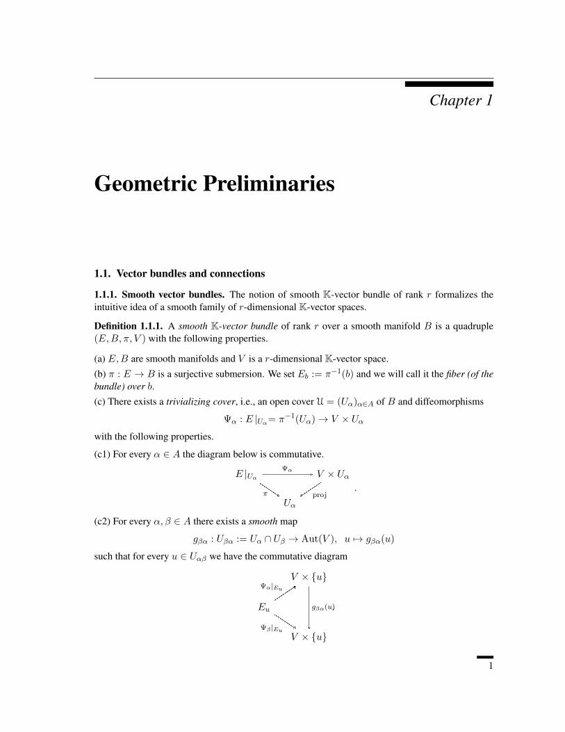
(c) There exists a trivializing cover, i.e., an open cover U = (Uα)α∈A of B and diffeomorphisms
Ψα : E |Uα= π−1(Uα)→ V × Uαwith the following properties.
(c1) For every α ∈ A the diagram below is commutative.
E |Uα V × Uα
Uα
''')
π
wΨα
[[[ proj
.
(c2) For every α, β ∈ A there exists a smooth map
gβα : Uβα := Uα ∩ Uβ → Aut(V ), u 7→ gβα(u)
such that for every u ∈ Uαβ we have the commutative diagram
V × u
Eu
V × uu
gβα(u)[[[]
Ψα|Eu
''')
Ψβ |Eu
.
1

2 Liviu I. Nicolaescu
B is called the base, E is called total space, V is called the model (standard) fiber and π is calledthe canonical (or natural) projection. A K-line bundle is a rank 1 K-vector bundle.
Remark 1.1.2. The condition (c) in the above definition implies that each fiber Eb has a naturalstructure of K-vector space. Moreover, each map Ψα induces an isomorphism of vector spaces
Ψα |Eb→ V × b.ut
Here is some terminology we will use frequently. Often instead of (E, π,B, V ) we will writeE
π→ B or simply E. The inverses of Ψ−1α are called local trivializations of the bundle (over Uα).
The map gβα is called the gluing map from the α-trivialization to the β-trivialization. The collectiongβα : Uαβ → Aut(V ); Uαβ 6= ∅
is called a (Aut(V ))-gluing cocycle (subordinated to U) since it satisfies the cocycle condition
gγα(u) = gγβ(u) · gβα(u), ∀u ∈ Uαβγ := Uα ∩ Uβ ∩ Uγ , (1.1.1)
where ”·” denotes the multiplication in the Lie group Aut(V ). Note that (1.1.1) implies that
gαα(u) ≡ 1V , gβα(u) = gαβ(u)−1, ∀u ∈ Uαβ. (1.1.2)
Example 1.1.3. (a) A vector space can be regarded as a vector bundle over a point.
(b) For every smooth manifold M and every finite dimensional K-vector space we denote by VM
the trivial vector bundleV ×M →M, (v,m) 7→ m.
(c) The tangent bundle TM of a smooth manifold is a smooth vector bundle.
(d) If E π→ B is a smooth vector bundle and U → B is an open set then E |Uπ→ U is the vector
bundleπ−1(U)
π→ U.
(e) Recall that CP1 is the space of all one-dimensional subspaces of C2. Equivalently, CP1 is thequotient of C2 \ 0 modulo the equivalence relation
p ∼ p′ ⇐⇒ ∃λ ∈ C∗ : p′ = λp.
For every p = (z0, z1) ∈ C2 \ 0 we denote by [p] = [z0, z1] its ∼-equivalence class which weview as the line containing the origin and the point (z0, z1). We have a nice open cover U0, U1 ofCP1 defined by
Ui := [z0, z1]; zi 6= 0.The setU0 consists of the lines transversal to the vertical axis, whileU1 consists of the lines transver-sal to the horizontal axis. The slope m0 = z1/z0 of the line through (z0, z1) is a local coordinatedover U0 and the slope m1 = z0/z1 is a local coordinate over U1. On the overlap we have
m1 = 1/m0.
LetE = (x, y; [z0, z1]) ∈ C2 × CP1;
y
x=z1
z0, i.e. yz0 − xz1 = 0
The natural projection C2×CP1 → CP1 induces a surjection π : E → CP1. Observe that for every[p] ∈ CP1 the fiber π−1(p) can be naturally identified with the line through p. We can thus regard

Notes on the Atiyah-Singer index Theorem 3
E as a family of 1-dimensional vector spaces. We want to show that π actually defines a structureof a smooth complex line bundle over CP1. Set
Ei := π−1(Ui) =
(x, y; [z0, z1]) ∈ E; zi 6= 0.
We construct a map
Ψ0 : E0 → C× U0, E0 3 (x, y; [z0, z1]) 7→ (x, [z0, z1])
andΨ1 : E1 → C× U1, E1 3 (x, y; [z0, z1]y) 7→ (y, [z0, z1])
Observe that Ψ0 is bijective with inverse Ψ−10 : C× U0 → E0 is given by
C× U0 3 (t; [z0, z1]) 7→ (t,z1
z0t; [z0, z1]) = (t,m0t; [z0, z1]).
The compositionΨ1 Ψ−1
0 : C× U01 → C× U01
is given byC× U01 3 (s; [p]) 7→ (g10([p])s, [p]),
whereU01 3 [p] = [z0, z1] 7→ g10([p]) = z1/z0 = m0([p]) ∈ C∗ = GL1(C).
The complex line bundle constructed above is called the tautological line bundle. ut
Given a smooth manifold B, a vector space V , an open cover U = (Uα)α∈A of B, and a gluingcocycle subordinated to U
gβα : Uαβ → Aut(V )
we can construct a smooth vector bundle as follows. Consider the disjoint union
X =∐α∈A
V Uα .
Denote by E the quotient space of X modulo the equivalence relation
V Uα 3 (vα, uα) ∼ (vβ, uβ) ∈ V Uβ⇐⇒ uα = uβ = u ∈ Uαβ, vβ = gβα(u)vα.
Since we glue open sets of smooth manifolds via diffeomorphisms we deduce that E is naturally asmooth manifold. Moreover, the natural projections πα : V Uα → Uα are compatible with the aboveequivalence relation and define a smooth map
π : E → B.
The natural maps Φα : V Uα → E |Uα are diffeomorphisms and their inverses Ψα = Φ−1α satisfy
all the conditions in Definition 1.1.1. We will denote the vector bundle obtained in this fashion by(U, g••, V ) or by (B,U, g••, V ).
Definition 1.1.4. Suppose (E, πE , B, V ) and (F, πF , B,W ) are smooth K-vector bundles over Bof ranks p and respectively q. Assume Uα,Ψαα is a trivializing cover for πE and Vβ,Φββ is atrivializing cover for πF . A vector bundle morphism from E
πE−→ B to F πF−→ B is a smooth mapT : E → F satisfying the following conditions.
4 Liviu I. Nicolaescu
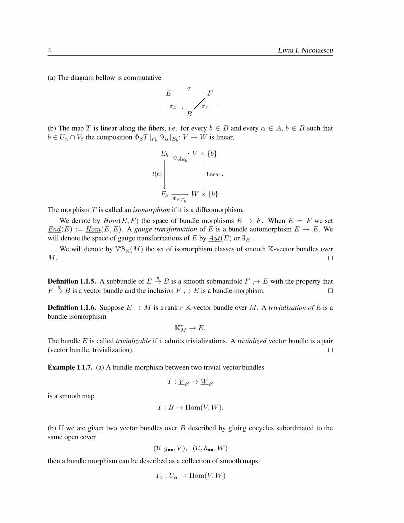
(a) The diagram bellow is commutative.
E F
B
wT
[[]πE
πF.
(b) The map T is linear along the fibers, i.e. for every b ∈ B and every α ∈ A, b ∈ B such thatb ∈ Uα ∩ Vβ the composition ΦβT |Fb Ψα |Eb : V →W is linear,
Eb V × b
Fb W × bu
T|Eb
wΨα|Eb
u
linear
wΦβ|Fb
.
The morphism T is called an isomorphism if it is a diffeomorphism.
We denote by Hom(E,F ) the space of bundle morphisms E → F . When E = F we setEnd(E) := Hom(E,E). A gauge transformation of E is a bundle automorphism E → E. Wewill denote the space of gauge transformations of E by Aut(E) or GE .
We will denote by VBK(M) the set of isomorphism classes of smooth K-vector bundles overM . ut
Definition 1.1.5. A subbundle of E π→ B is a smooth submanifold F → E with the property thatF
π→ B is a vector bundle and the inclusion F → E is a bundle morphism. ut
Definition 1.1.6. Suppose E → M is a rank r K-vector bundle over M . A trivialization of E is abundle isomorphism
KrM → E.
The bundle E is called trivializable if it admits trivializations. A trivialized vector bundle is a pair(vector bundle, trivialization). ut
Example 1.1.7. (a) A bundle morphism between two trivial vector bundles
T : V B →WB
is a smooth map
T : B → Hom(V,W ).
(b) If we are given two vector bundles over B described by gluing cocycles subordinated to thesame open cover
(U, g••, V ), (U, h••,W )
then a bundle morphism can be described as a collection of smooth maps
Tα : Uα → Hom(V,W )
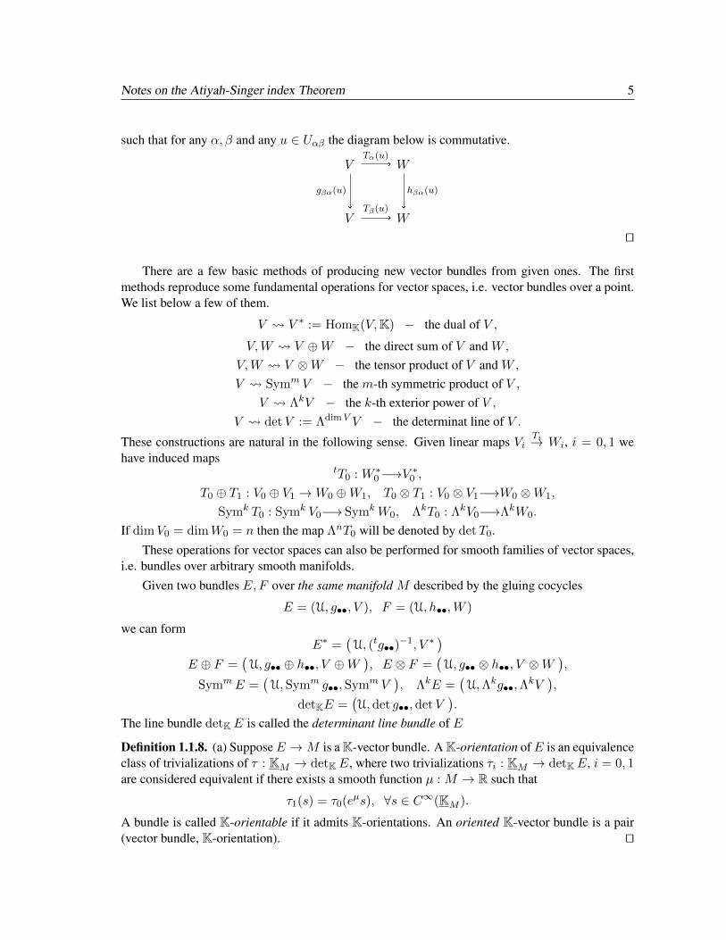
Notes on the Atiyah-Singer index Theorem 5
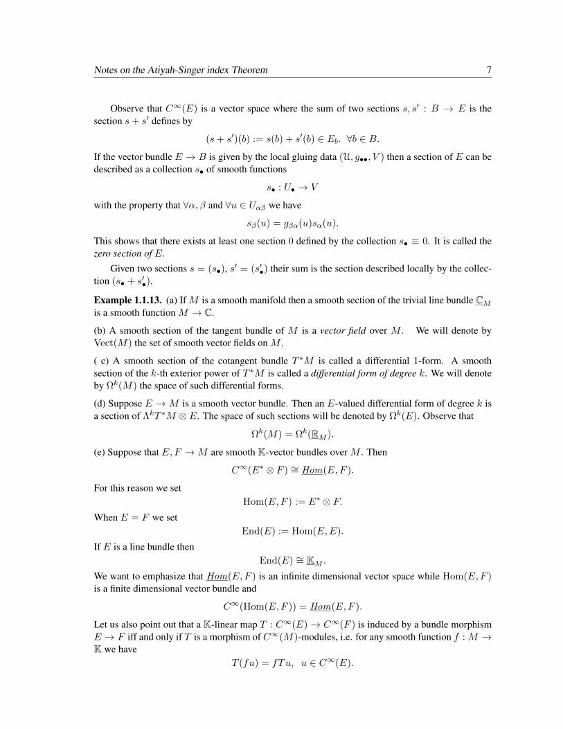
such that for any α, β and any u ∈ Uαβ the diagram below is commutative.
V W
V W
wTα(u)
ugβα(u)
uhβα(u)
wTβ(u)
ut
There are a few basic methods of producing new vector bundles from given ones. The firstmethods reproduce some fundamental operations for vector spaces, i.e. vector bundles over a point.We list below a few of them.
V V ∗ := HomK(V,K) − the dual of V ,
V,W V ⊕W − the direct sum of V and W,
V,W V ⊗W − the tensor product of V and W,
V Symm V − the m-th symmetric product of V ,V ΛkV − the k-th exterior power of V ,
V detV := ΛdimV V − the determinat line of V .
These constructions are natural in the following sense. Given linear maps ViTi→ Wi, i = 0, 1 we
have induced mapstT0 : W ∗0−→V ∗0 ,
T0 ⊕ T1 : V0 ⊕ V1 →W0 ⊕W1, T0 ⊗ T1 : V0 ⊗ V1−→W0 ⊗W1,
Symk T0 : Symk V0−→ SymkW0, ΛkT0 : ΛkV0−→ΛkW0.
If dimV0 = dimW0 = n then the map ΛnT0 will be denoted by detT0.
These operations for vector spaces can also be performed for smooth families of vector spaces,i.e. bundles over arbitrary smooth manifolds.
Given two bundles E,F over the same manifold M described by the gluing cocycles
E = (U, g••, V ), F = (U, h••,W )
we can formE∗ =
(U, (tg••)
−1, V ∗)
E ⊕ F =(U, g•• ⊕ h••, V ⊕W
), E ⊗ F =
(U, g•• ⊗ h••, V ⊗W
),
SymmE =(U, Symm g••, Symm V
), ΛkE =
(U,Λkg••,Λ
kV),
detKE =(U,det g••,detV
).
The line bundle detKE is called the determinant line bundle of E
Definition 1.1.8. (a) SupposeE →M is a K-vector bundle. A K-orientation ofE is an equivalenceclass of trivializations of τ : KM → detKE, where two trivializations τi : KM → detKE, i = 0, 1are considered equivalent if there exists a smooth function µ : M → R such that
τ1(s) = τ0(eµs), ∀s ∈ C∞(KM ).
A bundle is called K-orientable if it admits K-orientations. An oriented K-vector bundle is a pair(vector bundle, K-orientation). ut
6 Liviu I. Nicolaescu
Example 1.1.9. (a) A smooth manifold M is orientable if its tangent bundle TM is R-orientable.ut
When K = R and when no confusion is possible we will use the simpler terminology of orien-tation rather than R-orientation.
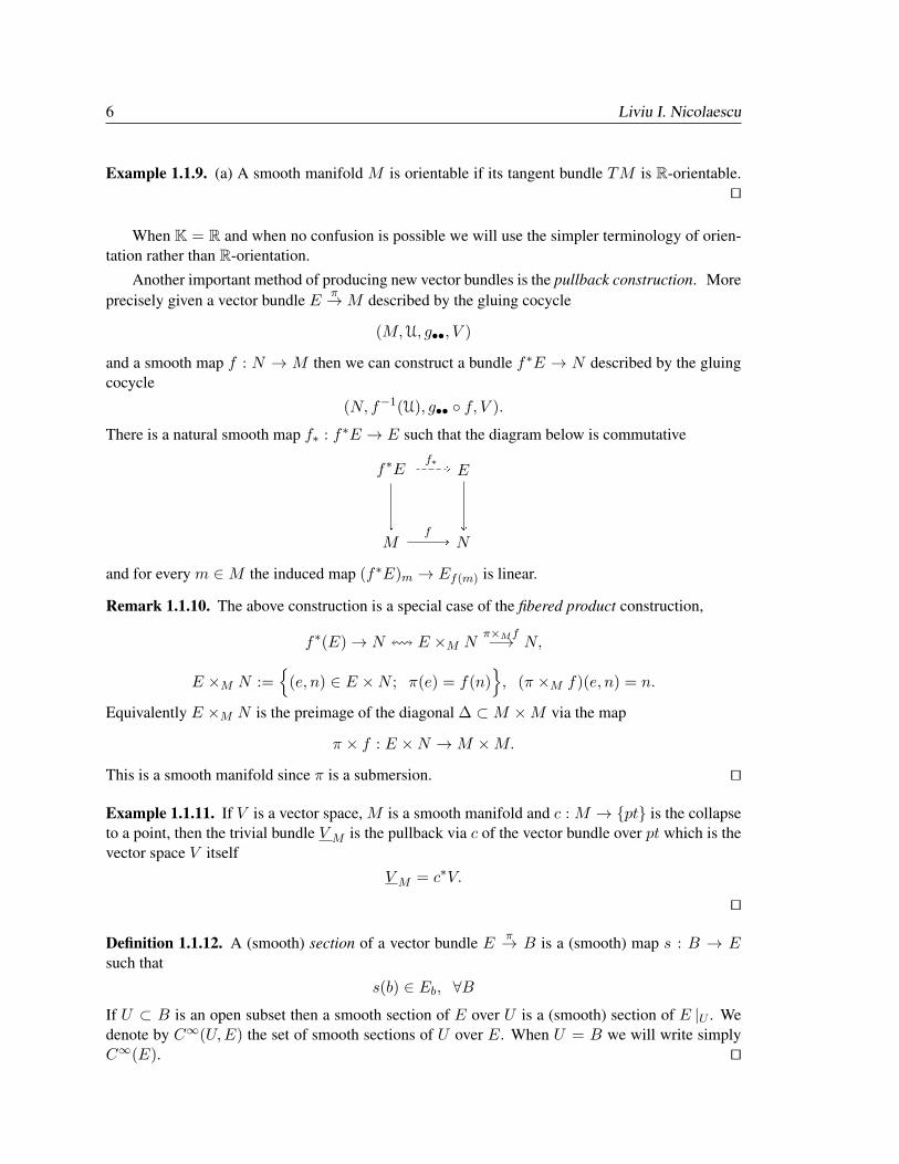
Another important method of producing new vector bundles is the pullback construction. Moreprecisely given a vector bundle E π→M described by the gluing cocycle
(M,U, g••, V )
and a smooth map f : N → M then we can construct a bundle f∗E → N described by the gluingcocycle
(N, f−1(U), g•• f, V ).
There is a natural smooth map f∗ : f∗E → E such that the diagram below is commutative
f∗E E
M N
wf∗
u uw
f
and for every m ∈M the induced map (f∗E)m → Ef(m) is linear.
Remark 1.1.10. The above construction is a special case of the fibered product construction,
f∗(E)→ N! E ×M Nπ×Mf−→ N,
E ×M N :=
(e, n) ∈ E ×N ; π(e) = f(n), (π ×M f)(e, n) = n.
Equivalently E ×M N is the preimage of the diagonal ∆ ⊂M ×M via the map
π × f : E ×N →M ×M.
This is a smooth manifold since π is a submersion. ut
Example 1.1.11. If V is a vector space, M is a smooth manifold and c : M → pt is the collapseto a point, then the trivial bundle VM is the pullback via c of the vector bundle over pt which is thevector space V itself
VM = c∗V.
ut
Definition 1.1.12. A (smooth) section of a vector bundle E π→ B is a (smooth) map s : B → Esuch that
s(b) ∈ Eb, ∀B
If U ⊂ B is an open subset then a smooth section of E over U is a (smooth) section of E |U . Wedenote by C∞(U,E) the set of smooth sections of U over E. When U = B we will write simplyC∞(E). ut
Notes on the Atiyah-Singer index Theorem 7
Observe that C∞(E) is a vector space where the sum of two sections s, s′ : B → E is thesection s+ s′ defines by
(s+ s′)(b) := s(b) + s′(b) ∈ Eb. ∀b ∈ B.
If the vector bundle E → B is given by the local gluing data (U, g••, V ) then a section of E can bedescribed as a collection s• of smooth functions
s• : U• → V
with the property that ∀α, β and ∀u ∈ Uαβ we have
sβ(u) = gβα(u)sα(u).
This shows that there exists at least one section 0 defined by the collection s• ≡ 0. It is called thezero section of E.
Given two sections s = (s•), s′ = (s′•) their sum is the section described locally by the collec-tion (s• + s′•).
Example 1.1.13. (a) If M is a smooth manifold then a smooth section of the trivial line bundle CMis a smooth function M → C.
(b) A smooth section of the tangent bundle of M is a vector field over M . We will denote byVect(M) the set of smooth vector fields on M .
( c) A smooth section of the cotangent bundle T ∗M is called a differential 1-form. A smoothsection of the k-th exterior power of T ∗M is called a differential form of degree k. We will denoteby Ωk(M) the space of such differential forms.
(d) Suppose E → M is a smooth vector bundle. Then an E-valued differential form of degree k isa section of ΛkT ∗M ⊗ E. The space of such sections will be denoted by Ωk(E). Observe that
Ωk(M) = Ωk(RM ).
(e) Suppose that E,F →M are smooth K-vector bundles over M . Then
C∞(E∗ ⊗ F ) ∼= Hom(E,F ).
For this reason we setHom(E,F ) := E∗ ⊗ F.
When E = F we setEnd(E) := Hom(E,E).
If E is a line bundle thenEnd(E) ∼= KM .
We want to emphasize that Hom(E,F ) is an infinite dimensional vector space while Hom(E,F )is a finite dimensional vector bundle and
C∞(Hom(E,F )) = Hom(E,F ).
Let us also point out that a K-linear map T : C∞(E)→ C∞(F ) is induced by a bundle morphismE → F iff and only if T is a morphism of C∞(M)-modules, i.e. for any smooth function f : M →K we have
T (fu) = fTu, u ∈ C∞(E).
8 Liviu I. Nicolaescu
(e) Suppose thatE →M is a real vector bundle. A metric onE is then a section h of Sym2E∗ withthe property that for every m ∈ M the symmetric bilinear form hm ∈ Sym2E∗ is an Euclideanmetric on the fiber Em. A Riemann metric on a manifold M is a metric on the tangent bundle TM .A metric on E induces metrics on all the bundles E∗, E⊗k, Symk E, ΛkE.
Observe that if h is a metric on E and F is a sub-bundle of E then h induces a metric on F . Inparticular, the tautological line bundle L → CP1 is by definition a subbundle of the trivial vectorbundle C2
CP1 and as such it is equipped with a natural metric.
(f) Suppose thatE →M is a complex vector of rank r described by the gluing cocycle (U, g••,Cr).Then the conjugate ofE is the complex vector bundle E described by the gluing cocycle (U, g••,Cr)where for any matrix g ∈ GLr(C) we have denoted by g its complex conjugate. Note that thereexists a canonical isomorphism of real vector bundles
C : E → E
called the conjugation.
A section u of E∗ defines for every m ∈ M a R-linear map um : Em → C which is complexconjugate linear i.e.
um(λe) = λum(e), ∀e ∈ Em, λ ∈ C.A hermitian metric on H is a section h of E∗ ⊗C E
∗ satisfying for every m ∈ M the followingproperties.
hm defines a R-bilinear map E×E → C which is complex linear in the first variable and conjugatelinear in the second variable.
hm(e1, e2) = h(e2, e1), ∀e1, e2 ∈ Em.
hm(e, e) > 0, ∀e ∈ Em \ 0.If E is a vector bundle equipped with a metric h (riemannian or hermitian), then we denote byEnd−h (E) the real subbundle of End(E) whose sections are the endomorphisms T : E → Esatisfying
h(Tu, v) = −h(u, Tv), ∀u, v ∈ C∞(E).
(g) A K-vector bundle is K-orientable iff detKE admits a nowhere vanishing section. Indeed sincedetKE ∼= (KM )∗ ⊗ detKE ∼= Hom(KM , E) a section of E can be identified with a bundlemorphism KM → E. This is an isomorphism since the section is nowhere vanishing.
(h) Every complex vector bundle E → M is R-orientable. To construct it we need to produce anowhere vanishing section of detRE. Suppose E is described by the gluing cocycle (U, g••,Cr).Using the inclusion
i : GLr(C) → GL2r(R)
we get mapsg•• = i g•• : U•• → GL2r(R)
satisfyingw•• := det g•• = | det g••|2 > 0.
Letf•• := logw•• ⇐⇒ w•• = exp(f••).
Notes on the Atiyah-Singer index Theorem 9
Since w•• defines a gluing cocycle for detRE and in particular
wγα(u) = wγβ(u)wβα(u).
We deducefγα(u) = fγβ(u) + fβα(u), ∀α, β, γ, ∀u ∈ Uαβγ .
Consider now a partition of unity (θα) subordinated to U, supp θα ⊂ Uα. Define
fα : Uα → R, fα(u) =∑Uβ3u
θβ(u)fβα(u) =∑β
θβ(u)fβα(u)
Observe first that fα is smooth. Using the equalities
fγα − fγβ = fγα + fβγ = fβα
we deduce1
fα − fβ =∑γ
θγ(fγα − fγβ) =∑γ
θγfβα =(∑
γ
θγ
)fβα = fβα.
Equivalently−fβ = fβα − fα =⇒ e−fβ = wβαe
−fα = (det gβα)e−fα .
This shows that the collection sα = e−fα is a nowhere vanishing section of detRE.
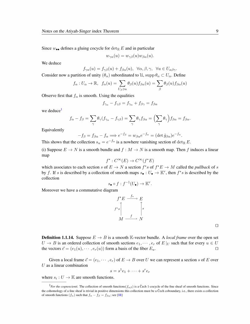
(i) Suppose E → N is a smooth bundle and f : M → N is a smooth map. Then f induces a linearmap
f∗ : C∞(E)→ C∞(f∗E)
which associates to each section s of E → N a section f∗s of f∗E → M called the pullback of sby f . If s is described by a collection of smooth maps s• : U• → Kr, then f∗s is described by thecollection
s• f : f−1(U•)→ Kr.
Moreover we have a commutative diagram
f∗E E
M N
wf∗
u
f∗s
wf
u
s
ut
Definition 1.1.14. Suppose E → B is a smooth K-vector bundle. A local frame over the open setU → B is an ordered collection of smooth sections e1, · · · , er of E |U such that for every u ∈ Uthe vectors ~e = (e1(u), · · · , er(u)) form a basis of the fiber Eu. ut
Given a local frame ~e = (e1, · · · , er) of E → B over U we can represent a section s of E overU as a linear combination
s = s1e1 + · · ·+ srer
where si : U → K are smooth functions.
1For the cognoscienti. The collection of smooth functions(fαβ) is a Cech 1-cocycle of the fine sheaf of smooth functions. Sincethe cohomology of a fine sheaf is trivial in positive dimensions this collection must be a Cech coboundary, i.e., there exists a collectionof smooth functions (fα) such that fα − fβ = fβα; see [11]
10 Liviu I. Nicolaescu
1.1.2. Principal bundles. Fix a Lie group G. For simplicity, we will assume that it is a matrix Liegroup2, i.e. it is a closed subgroup of some GLn(K). A principal G-bundle over a smooth manifoldB is a triple (P, π,B) satisfying the following conditions.
Pπ→ B
is a surjective submersion. We set Pb := π−1b
There is a right free actionP ×G→ P, (p, g) 7→ pg
such that for every p ∈ P the G-orbit containing p coincides with the fiber of π containing p.
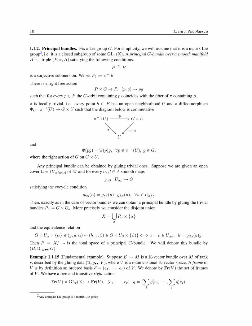
π is locally trivial, i.e. every point b ∈ B has an open neighborhood U and a diffeomorphismΨU : π−1(U)→ G× U such that the diagram below is commutative
π−1(U) G× U
U
wΨ
[[[]π
proj
andΨ(pg) = Ψ(p)g, ∀p ∈ π−1(U), g ∈ G,
where the right action of G on G× U .
Any principal bundle can be obtained by gluing trivial ones. Suppose we are given an opencover U = (Uα)α∈A of M and for every α, β ∈ A smooth maps
gαβ : Uαβ → G
satisfying the cocycle condition
gγα(u) = gγβ(u) · gβα(u), ∀u ∈ UαβγThen, exactly as in the case of vector bundles we can obtain a principal bundle by gluing the trivialbundles Pα = G× Uα. More precisely we consider the disjoint union
X =⋃α
Pα × α
and the equivalence relation
G× Uα × α 3 (g, u, α) ∼ (h, v, β) ∈ G× Uβ × β) ⇐⇒ u = v ∈ Uαβ, h = gβα(u)g.
Then P = X/ ∼ is the total space of a principal G-bundle. We will denote this bundle by(B,U, g••, G).
Example 1.1.15 (Fundamental example). Suppose E → M is a K-vector bundle over M of rankr, described by the gluing data (U, g••, V ), where V is a r-dimensional K-vector space. A frame ofV is by definition an ordered basis ~e = (e1, · · · , er) of V . We denote by Fr(V ) the set of framesof V . We have a free and transitive right action
Fr(V )×GLr(K)→ Fr(V ), (e1, · · · , er) · g = (∑i
gi1ei, · · · ,∑i
girei),
2Any compact Lie group is a matrix Lie group
Notes on the Atiyah-Singer index Theorem 11
∀g = [gij ]1≤i,j≤r ∈ GLr(K), (e1, · · · , er) ∈ Fr(V ).
In particular, the set of frames is naturally a smooth manifold diffeomorphic to GLr(K). Note that aframe ~e of V associates to every vector v ∈ V a vector v(~e) ∈ Kr, the coordinates of v with respectto the frame ~e. For every g ∈ GLr(K) we have
v(~e · g) = g−1v(~e).
If we let GLr(K) act on the right on Kr,
Kr ×GLr(K) 3 (u, g) 7→ u · g = g−1u ∈ Kr
then we see that the coordinate map induced by v ∈ V ,
v : Fr(V )→ Kr, ~e→ v(~e)
is G-equivariant.
An isomorphism Ψ : V → Kr induces a diffeomorphism~Φ : GLr(K)→ Fr (V ), g 7→ ~Φ(g) = Ψ−1(~δ) · g,
where ~δ denotes the canonical frame of Kr. Observe that~Φ(g · h) = ~Φ(g) · h.
To the bundleE we associate the principal bundle Fr (E) given by the gluing cocycle (U, g••,GLr(K)).The fiber of this bundle over m ∈ Uα can be identified with the space Fr(Em) of frames in the fiberEm via the map ~Φ and the local trivialization
Ψα : Em → Kr. ut
To any principal bundle P = (B,U, g••, G) and representation ρ : G → AutK(V ) of G on afinite dimensional K-vector space V we can associate a vector bundle E = (B,U, ρ(g••), V ). Wewill denote it by P ×ρ V . Equivalently, P ×ρ V is the quotient of P × V via the left G-action
g(p, v) = (pg−1, ρ(g)v).
A vector bundle E on a smooth manifold M is said to have (G, ρ)-structure if E ∼= P ×ρ V forsome principal G-bundle P .
We denote by g = T1G the Lie algebra of G. We have an adjoint representation
Ad : G→ End g, Ad(g)X = gXg−1 =d
dt|t=0 g exp(tX)g−1, ∀g ∈ G.
The associated vector bundle P ×Ad g is denoted by Ad(P ).
For any representation ρ : G→ Aut(V ) we denote by ρ∗ the differential of ρ at 1
ρ∗ : g→ EndV.
Observe that for every X ∈ g we have
ρ∗(Ad(g)X) = ρ∗(gXg−1) = ρ(g)(ρ∗X)ρ(g)−1. (1.1.3)
If we set Endρ V := ρ∗(g) ⊂ EndV we have an induced action
Adρ : G→ Endρ(V ), Adρ(g)T := ρ(g)Tρ(g)−1, ∀T ∈ EndV, g ∈ G.If E = P ×ρ V then we set
Endρ(V ) := P ×Adρ Endρ(V ).
This bundle can be viewed as the bundle of infinitesimal symmetries of E.

12 Liviu I. Nicolaescu
Example 1.1.16. (a) Suppose G is a Lie subgroup of GLm(K). It has a tautological representation
τ : G → GLm(K) = Aut(Km).
A rank m K-vector bundle E → M is said to have G-structure if it has a (G, τ)-structure. Thismeans that E can be described by a gluing cocycle (U, g••,Km) with the property that the matricesg•• belong to the subgroup G.
For example, SO(m),O(m) ⊂ GLm(R) and we can speak of SO(m) and O(m) structures on areal vector bundle of rank m. Similarly we can speak of U(m) and SU(m) structures on a complexvector bundle of rank m.
A hermitian metric on a rank r complex vector bundle defines a U(r)-structure on E and in thiscase
AdP = Endρ(E) = End−h (E). ut
1.1.3. Connections on vector bundles. Roughly speaking, a connection on a smooth vector bundleis a ”coherent procedure” of differentiating the smooth sections.
Definition 1.1.17. Suppose E →M is a K-vector bundle. A smooth connection on E is a K-linearoperator
∇ : C∞(E)→ C∞(T ∗M ⊗ E)
satisfying the product rule
∇(fs) = s⊗ df + f∇s, ∀f ∈ C∞(M), s ∈ C∞(E).
We say that ∇s is the covariant derivative of s with respect to ∇. We will denote by AE the spaceof smooth connections on E. ut
Remark 1.1.18. (a) For every section s ofE the covariant derivative∇s is a section of T ∗M⊗E ∼=Hom(TM,E). i.e.
∇s ∈ Hom(TM,E).
As such, ∇s associates to each vector field X on M a section of E which we denote by ∇Xs. Wesay that∇Xs is the derivative of s in along the vector field X with respect to the connection∇. Theproduct rule can be rewritten
∇X(fs) = (LXf)s+ f∇s, ∀X ∈ Vect(M), f ∈ C∞(M), s ∈ C∞(M),
where LXf denotes the Lie derivative of f along the vector field X .
(b) Suppose E,F → M are vector bundles and Ψ : E → F is a bundle isomorphism. If ∇ is aconnection of E then Ψ∇Ψ−1 is a connection on F .
(c) Suppose∇0 and ∇1 are two connections on E. Set
A := ∇1 −∇0 : C∞(E)→ C∞(T ∗M × E).
Observe that for every f ∈ C∞(M) and every s ∈ C∞(E) we have
A(fs) = fA(s)
so that
A ∈ Hom(E, T ∗M ⊗ E) ∼= C∞(E∗ ⊗ T ∗M ⊗ E) ∼= C∞(T ∗M ⊗ E∗ ⊗ E)
∼= C∞(TM,End(E)
)= Ω1(End(E)).
Notes on the Atiyah-Singer index Theorem 13
In other words, the difference between two connections is a EndE-valued 1-form. Conversely, if
A ∈ Ω1(EndE) ∼= Hom(TM ⊗ E,E)
then for every connection ∇ on E the sum ∇+A is a gain a connection on E. This shows that thespace AE , if nonempty, is an affine space modelled by the vector space Ω1(EndE). ut
Example 1.1.19. (a) Consider the trivial bundle RM . The sections of RM are smooth functionsM → R. The differential
d : C∞(M)→ Ω1(M), f 7→ df
is a connection on RM called the trivial connection.
Observe that End(RM ) ∼= RM so that any other connection on M has the form
∇ = d+ a, a ∈ Ω1(RM ) = Ω1(M).
(b) Consider similarly the trivial bundle KrM . Its smooth sections are r-uples of smooth functions
s =
s1
...sr
: M → Kr.
Kr is equipped with a trivial connection∇0 defined by
∇0
s1
...sr
=
ds1
...dsr
.Any other connection on Kr has the form
∇ = ∇0 +A, A ∈ Ω1(EndKr).
More concretely, A is an r × r matrix [Aab ]1≤a,b≤r, where each entry Aab is a K-valued 1-form. Ifwe choose local coordinates (x1, · · · , xn) on M then we can describe Aij locally as
Aab =∑k
Aakbdxk.
We have
∇s =
ds1
...dsr
+
∑
bA1bsb
...
...∑bA
rbsb
.(c) Suppose E → B is a K-vector bundle of rank r and ~e = (e1, · · · , er) is a local frame of E overthe open set U . Suppose ∇ is a connection on E. Then for every 1 ≤ b ≤ r we get section ∇eb ofT ∗M ⊗ E over U and thus decompositions
∇eb =∑a
Aabea, Aab ∈ Ω1(U), ∀1 ≤ a, b ≤ r. (1.1.4)
Given a section s =∑b sbeb of E over U we have
∇s =∑b
dsbeb +∑b
sb∑a
Aabea =∑a
(dsa +
∑b
Aabsb)ea.
14 Liviu I. Nicolaescu
This shows that the action of ∇ on any section over U is completely determined by the action of ∇on the local frame, i.e by the matrix (Aab ). We can regard this as a 1-form whose entries are r × rmatrices. This is known as the connection 1-form associated to ∇ by the local frame ~e. We willdenote it by A(~e). We can rewrite (1.1.4) as
∇(~e) = ~e ·A(~e).
Suppose ~f = (f1, · · · , fr) is another local frames of E over U related to ~e by the equalities
fa =∑b
ebgba, (1.1.5)
where U 3 u 7→ g(u) = (gba(u))1≤a,b≤r ∈ GLr(K) is a smooth map. We can rewrite (1.1.5) as
~f = ~e · g.
Then A(~f) is related to A(~e) by the equality
A(~f) = g−1A(~e)g + g−1dg. (1.1.6)
Indeed
~f ·A(~f) = ∇(~f) = ∇(~eg) = (∇(~e))g + ~edg = (~eA(~e))g + ~fg−1dg = ~f(g−1A(~e)g + g−1dg).
Suppose now that E is given by the gluing cocycle (U, g••, ,Kr). Then the canonical basis of Kr
induces via the natural isomorphism KrUα → E |Uα a local frame ~e(α) of E |Uα . We set
Aα = A(~e(α)).
Observe that Aα is a 1-form with coefficients in glr(K) = End(Kr), the Lie algebra GLr(K). On
the overlap Uαβ we have the equality ~e(α) = ~e(β)gβα so that on these overlaps the glr(K)-valued
1-forms Aα satisfy the transition formulæ
Aα = g−1βαAβgβα + g−1
βαdgβα ⇐⇒ Aβ = gβαAαg−1βα − (dgβα)g−1
βα . (1.1.7)
ut
Proposition 1.1.20. Suppose E is a rank r vector bundle over M described by the gluing cocycle(U, g••,Kr). Then a collection of 1-forms
Aα ∈ Ω1(Uα)⊗ glr(K).
satisfying the gluing conditions (1.1.7) determine a connection on E. ut
Proposition 1.1.21. Suppose E → M is a smooth vector bundle. Then there exist connections onE, i.e. AE 6= ∅.
Proof. Suppose that E is described by the gluing cocycle (U, g••,Kr), r = rank(E).
Denote by Ψα : KrUα → E |Uα the local trivialization over Uα and by ∇α the trivial connection
on KrUα Set
∇α := Ψα∇αΨ−1α .

Notes on the Atiyah-Singer index Theorem 15
Then (see Remark 1.1.18(b)) ∇α is a connection onE |Uα . Fix a partition of unity (θα) subordinatedto (Uα). Observe that for every α, and every s ∈ C∞(E), θαs is a section of E with support in Uα.In particular ∇α(θαs) is a section of T ∗M ⊗ E with support in Uα. Set
∇s =∑α,β
θβ∇α(θαs)
If f ∈ C∞(M) then
∇(fs) =∑α,β
θβ∇α(θαfs) =∑β
θβ
(∑α
df ⊗ (θαs) + f∇α(θαs))
= df ⊗ s∑α,β
θαθβ + f∇s = df ⊗ s(∑
αθα︸ ︷︷ ︸
=1
)(∑βθβ︸ ︷︷ ︸
=1
)+ f∇s = df ⊗ s+ f∇s.
Hence∇ is a connection on E. ut
Definition 1.1.22. Suppose Ei → M , i = 0, 1 are two smooth vector bundles over M . Supposealso ∇i is a connection on Ei, i = 0, 1. A morphism (E0,∇0) → (E1,∇1) is a bundle morphismT : E0 → E1 such that for every X ∈ Vect(M) the diagram below is commutative.
C∞(E0) C∞(E1)
C∞(E0) C∞(E1)
wT
u∇0X
u∇1X
wT
An isomorphism of vector bundles with connections is defined in the obvious way. We denote byVBc
K(M) the collection of isomorphism classes of K-vector bundles with connections over M . ut
Observe that we have a forgetful map
VBc(M)→ VB(M), (E,∇) 7→ E.
The tensorial operations ⊕, ∗, ⊗, S and Λ∗ on VB(M) have lifts to the richer category of vectorbundles with connections. We explain this construction in detail. Suppose (Ei,∇i) ∈ VBc(M),i = 0, 1.
•We obtain a connection∇ = ∇0 ⊕∇1 on E0 ⊕ E1 via the equality
∇(s0 ⊕ s1) = (∇0s0 ⊕∇1s1), ∀s0 ∈ C∞(E0), s1 ∈ C∞(E1).
• The connection∇0 induces a connection ∇0 on E∗0 defined by the equality
LX〈u, v〉 = 〈∇0Xu, v〉+ 〈u,∇Xv〉, ∀X ∈ Vect(M), u ∈ C∞(E∗0), v ∈ C∞(E0),
where 〈•, •〉 ∈ Hom(E∗0 ⊗ E0,KM ) denotes the natural bilinear pairing between a bundle and itsdual.
Suppose ~e = (e1, . . . , er) is a local frame of E and A(~e) is the connection 1-form associated to∇,
∇~e = ~e ·A(~e)
Denote by t~e = (e1, . . . , cer) the dual local frame of E∗0 defined by
〈ea, eb〉 = δab .
16 Liviu I. Nicolaescu
We deduce that 〈∇0ea, eb〉 = −〈ea,∇0eb〉 = −Aab so that
∇0ea = −∑b
Aabeb.
We can rewrite this∇0t~e = t~e ·
(−tA(~e)
)that is
A(t~e) = −tA(~e).
•We get a connection∇0 ⊗∇1 on E0 ⊗ E1 via the equality
(∇0 ⊗∇1)(s0 ⊗ s1) = (∇s0)⊗ s1 + s1 ⊗ (∇1s1).
•We get a connection on ΛkE0 via the equality
∇0X(s1∧· · ·∧sk) = (∇Xs1)∧s2∧· · ·∧sk+s1∧ (∇0
Xs2)∧· · ·∧sk+ · · ·+s1∧s2∧· · ·∧ (∇0Xsk)
∀s1, · · · , sk ∈ C∞(M), X ∈ Vect(M).
• If E is a complex vector bundle, then any connection ∇ on E induces a connection ∇ on theconjugate bundle E defined via the conjugation operator C : E → E
∇ = C∇C−1.
SupposeE → N is a vector bundle over the smooth manifoldN , f : M → N is a smooth map,and ∇ is a connection on E. Then ∇ induces a connection f∗∇ on f∗ defined as follows. If E isdefined by the gluing cocycle (U, g••,Kr) and∇ is defined by the collection A• ∈ Ω1(•)⊗ gl
r(K),
then f∇ is defined by the collection f∗A• ∈ Ω1(f−1(U•))⊗ glr(K). It is the unique connection on
f∗E which makes commutative the following diagram.
C∞(E) C∞(f∗E)
C∞(T ∗N ⊗ E) C∞(T ∗M ⊗ f∗E)
wf∗
u∇
uf∗∇
wf∗
Definition 1.1.23. Suppose∇ is a connection on the vector bundle E →M .
(a) A section s ∈ C∞(E) is called (∇)-covariant constant or parallel if
∇s = 0.
(b) A section s ∈ C∞(E) is said to be parallel along the smooth path γ : [0, 1]→M if the pullbacksection γ∗s of γ∗E → [0, 1] is parallel with respect to the connection f∗∇. ut
Example 1.1.24. Suppose γ : [0, 1] → M is a smooth path whose image lies entirely in a singlecoordinate chart U of M . Denote the local coordinates by (x1, . . . , xn) so we can represent γ as an-uple of functions (x1(t), · · · , xn(t)). Suppose E → M is a rank r vector bundle over M whichcan be trivialized over U . If∇ is a connection on E then with respect to some trivialization of E |Ucan be described as
∇ = d+A = d+∑i
dxi ⊗Ai, Ai : U → glr(K).
Notes on the Atiyah-Singer index Theorem 17
The tangent vector γ along γ can be described in the local coordinates as
γ =∑i
xi∂i.
A section s is the parallel along γ if ∇γs = 0. More precisely, if we regard s as a smooth functions : U → Kr, then we can rewrite this condition as
0 =d
dγs+
∑i
dxi(γ)Ais = (∑i
xi∂i)s+∑i
xiAis,
ds
dt+∑i
xiAis = 0. (1.1.8)
Thus a section which is parallel over a path γ(0) satisfies a first order linear differential equation.The existence theory for such equations shows that given any initial condition s0 ∈ Eγ(0) thereexists a unique parallel section [0, 1] 3 t 7→ S(t; s0) ∈ Eγ(t). We get a linear map
Eγ(0) 3 s0 → S(t; s0) |t=1∈ Eγ(1).
This is called the parallel transport along γ (with respect to the connection∇). ut
SupposeE is a real vector bundle, g is a metric onE. A connection∇ onE is called compatiblewith the metric g (or a metric connection) if g is a section ofE∗⊗E∗ covariant constant with respectto the connection on E∗⊗E∗ induced by∇. More explicitly, this means that for every sections u, vof E and every vector field X on M we have
LXg(u, v) = g(∇Xu, v) + g(u,∇Xv).
Observe that if ∇0,∇1 are two connections compatible with g and A = ∇1 − ∇0, then the aboveequality show that the endomorphism AX = ∇1 −∇0
X of E satisfies
g(AXu, v) + g(u,AXv) = 0, ∀u, v ∈ C∞(E).
In other words A ∈ Ω1(End−g (E)), where we recall that End−g (E) denotes the real vector vectorbundle whose sections are skew-hermitian endomorphisms of E; see Example 1.1.13 (f). One candefine in a similar fashion the connections on a complex vector bundle compatible with a hermitianmetric h.
Proposition 1.1.25. Suppose h is a metric (Riemannian or Hermitian) on the vector bundleE. Thenthere exists connections compatible with h. Moreover the space AE,h of connections compatiblewith h is an affine space modelled on the vector space Ω1(End−h (E)). ut
The proof follows by imitating the arguments in Remark 1.1.18 and Proposition 1.1.21.
Suppose that∇ is a connection on a vector bundle E →M . For any vector fields X,Y over Mwe get three linear operators
∇X ,∇Y ,∇[X,Y ] : C∞(E)→ C∞(E),
where [X,Y ] ∈ Vect(M) is the Lie bracket of X and Y . Form the linear operator
F∇(X,Y ) : C∞(E)→ C∞(E),
F∇(X,Y ) = ∇X∇Y −∇Y∇X −∇[X,Y ] = [∇X ,∇Y ]−∇[X,Y ].
18 Liviu I. Nicolaescu
Observe two things. First,F∇(X,Y ) = −F∇(Y,X).
Second, if f ∈ C∞(M) and s ∈ C∞(E) then
F∇(X,Y )(fs) = fF∇(X,Y )s = F∇(fX, Y )s = F∇(X, fY )s
so that for every X,Y ∈ Vect(M) the operator F∇(X,Y ) is an endomorphism of E and thecorrespondence
Vect(M)×Vect(M)→ End(E), (X,Y ) 7→ F∇(X,Y )
is C∞(M)-bilinear and skew-symmetric. In other words F∇(•, •) is a 2-form with coefficients inEndE, i.e., a section of Ω2(EndE).
Definition 1.1.26. The EndE-valued 2-form F∇(•, •) constructed above is called the curvature ofthe connection∇. ut
Example 1.1.27. (a) Consider the trivial vector bundle E = KrU , where U is an open subset in Rn.
Denote by (x1, · · · , xn) the Euclidean coordinates on U . Denote by d the trivial connection on E.Any connection∇ on E has the form
∇ = d+A = d+∑i
dxiAi, Ai : U → glr(K).
Set ∂i := ∂∂xi
,∇i = ∇∂i . Then for every s : U → Kr we have
F∇(∂i, ∂j)s = [∇i,∇j ]s = ∇i(∇js)−∇j(∇is)
= ∇i(∂js+Ajs)−∇j(∂is+Ais) = (∂i +Ai)(∂js+Ajs)− (∂j +Aj)(∂is+Ais)
=(∂iAj − ∂jAi + [Ai, Aj ]
)s.
Hence ∑i<j
F (∂i, ∂j)dxi ∧ dxj =
(∂iAj − ∂jAi + [Ai, Aj ]
)dxi ∧ dxj .
We can write this formally as
F∇ = dA+A ∧A = −∑i
dxid(Ai) +(∑
i
dxiAi)∧(∑j
dxjAj).
Observe that if r = 1, so that E is the trivial line bundle KU then we can identify gl1(K) ∼= K so
the components Ai are scalars. In particular [Ai, Aj ] = 0 so that in this case
F∇ = dA.
(b) If E is a vector bundle described by a gluing cocycle (U, g••,Kr) and ∇ is a connection de-scribed by the collection of 1-forms Aα ∈ Ω1(Uα)⊗ gl
r(K) satisfying (1.1.7) then the curvature of
∇ is represented by the collection of 2-forms
Fα = dAα +Aα ∧Aαsatisfying the compatibility conditions
Fβ = gβαFαg−1βα on Uαβ. (1.1.9)
Notes on the Atiyah-Singer index Theorem 19
(c) If ∇ is a connection on a complex line bundle L → M then its curvature F∇ can be identifiedwith a complex valued 2-form. If moreover, ∇ is compatible with a hermitian metric then iF∇ is areal valued 2-form. ut
We define an operation
∧ : Ωk(EndE)× Ω`(EndE)→ Ωk+`(EndE),
by setting(ωk ⊗ S) ∧ (η` ⊗ T ) = (ωk ∧ η`)⊗ (ST )
for any Ωk ∈ Ωk(M), η` ∈ Ω`(M), S, T ∈ End(E).
Using a connection∇ on E we can produce an exterior derivative
d∇ : Ωk(EndE)→ Ωk+1(EndE)
defined byd∇(ωk ⊗ S) = (dωk)⊗ S + (−1)k(ω ⊗ 1E) ∧∇EndES,
We have the following result.
Proposition 1.1.28. Suppose ∇′,∇ are two connections on the vector bundle E → M . Theirdifference B = ∇1 −∇0 is an EndE-valued 1-form. Then
F∇′ = F∇ + d∇B +B ∧B.
Proof. The result is local so we can assume E is the trivial bundle over an open subset M → Rn.Let r = rankE. We can write
∇ = d+A, ∇′ = d+A′, A,A′ ∈ Ω1(M)⊗ glr(K).
Then B = A′ −A,
F ′ = F∇′ = dA′ +A′ ∧A′, F = F∇ = dA+A ∧A
and thus
F ′ − F = d(A′ −A) + (A′ ∧A′)− (A ∧A) = d(A′ −A) + (A+B) ∧ (A+ Γ)−B ∧B
= dB +B ∧A+A ∧B +B ∧B.
In local coordinates d∇ we have (see Exercise 1.4.6)
d∇(∑i
dxi ⊗Bi) = −∑i
dxi ∧
∑j
dxj ⊗∇jBi
= −
∑i
dxi ∧
∑j
dxj ⊗ (∂jBi + [Aj , Bi])
=∑i<j
dxi ∧ dxj ⊗ (∂iBj − ∂jBi)−∑i,j
dxi ∧ dxj ⊗ (AjBi −BiAj)
20 Liviu I. Nicolaescu
= dB +
∑j
dxj ⊗Aj
∧(∑i
dxi ⊗Bi
)+
(∑i
dxi ⊗Bi
)∧
∑j
dxj ⊗Aj
= dB +A ∧B +B ∧A.
ut
Notes on the Atiyah-Singer index Theorem 21
1.2. Chern-Weil theory
1.2.1. Connections on principal G-bundles. In the sequel we will work exclusively with matrixLie groups, i.e. closed subgroups of some GLr(K).
Fix a (matrix) Lie groupG and a principalG-bundle P = (M,U, g••) over the smooth manifoldM . Denote by g = T1G the Lie algebra of G. A connection on P is a collection
A = Aα ∈ Ω1(Uα)⊗ g
satisfying the following conditions
Aβ(u) = gβα(u)Aα(u)g−1βα(u)− d(gβα)gβα(u)−1, ∀u ∈ Uαβ. (1.2.1)
We denote by AP the space of connections on P .
Proposition 1.2.1. AP is an affine space modelled on Ω1(AdP ).
Proof. We will show that given two connections (A1α), (A0
α) their differenceCα = A1α−Aα0 defines
a global section of Λ1T ∗M ⊗AdP , i.e. on the overlaps Uβα we have the equality
Cβ = Ad(gβα)Cα = gβαCαg−1βα .
This follows immediately by taking the difference of the transition equalities (1.2.1) for A1• and A0
•.ut
To formulate our next result let us introduce an operation
[−,−] : Ωk(Uα)⊗ g× Ω`(Uα)⊗ g→ Ωk+`(Uα)⊗ g,
[ωk ⊗X, η` ⊗ Y ] := (ωk ∧ η`)⊗ [X,Y ],
where [X,Y ]-denotes the Lie bracket in g, or in the case of a matrix Lie group, [X,Y ] = XY −Y Xis the commutator of the matrices X,Y . Let us point out that if A,B ∈ Ω1(Uα)⊗ g, then
[A,B] = A ∧B +B ∧A.
We defineFα := dAα +
1
2[Aα, Aα] = dAα +Aα ∧Aα ∈ Ω2(Uα)⊗ g.
For a proof of the following result we refer to [21, Chap.8].
Proposition 1.2.2. (a) The collection Fα defines a global section F (A) of Λ2T ∗M ⊗AdP , i.e. onthe overlaps Uαβ it satisfies the compatibility conditions,
Fβ = gβαFαg−1βα = Ad(gβα)Fα.
(b) (The Bianchi Identity)dFα + [Aα, Fα] = 0, ∀α.
ut
The 2-form F (A) ∈ Ω2(AdP ) is called the curvature of A.
Consider now a representation ρ : G → Aut(V ) and the vector bundle E = P ×ρ V . Denoteby ρ∗ the differential of ρ at 1 ∈ G
ρ∗ : g→ EndV.
22 Liviu I. Nicolaescu
We recall that Endρ(V ) = ρ∗g and EndρE = P ×Adρ Endρ(V ). The identity (1.1.3) shows thatany connection (Aα) on P defines a connection ∇ = (ρ∗Aα) on E. We say that this connection iscompatible with the (G, ρ)-structure. Observe that
F∇ |Uα= ρ∗Fα.
In particular F∇ ∈ Ω2(EndρE).
Example 1.2.3. Suppose E → M is a complex vector bundle of rank r. A hermitian metric h onE defines a U(r)-structure. A connection ∇ is compatible with this structure if and only if it iscompatible with the metric. In this case EndρE is the subbundle End−h E of EndE and we have
F (∇) ∈ Ω2(End−h E).
ut
1.2.2. The Chern-Weil construction. Suppose P → M is a principal G-bundle over M definedby the gluing cocycle (U, g••). To formulate the Chern-Weil construction we need to introduce firstthe concept of Ad-invariant polynomials on g. .
The adjoint representation Ad : G→ GL(g) induces an adjoint representation
Adk : G→ GL(Symk g∗C), gC := g⊗R C.
We denote by Ik(g) the Adk-invariant elements of Symk g∗. Equivalently, they are k-multilinearmaps
P : g× · · · × g︸ ︷︷ ︸k
→ C,
such thatP (Xϕ(1), . . . , Xϕ(k)) = P (gX1g
−1, . . . , gXkg−1) = P (X1, . . . , Xk),
for any X1, . . . , Xk ∈ g, g ∈ G and any permutation ϕ of 1, . . . , k.If in the above equality we take g = exp(tY ), Y ∈ g and then we differentiate with respect to t
at t = 0 we obtain
P ([Y,X1], X2, . . . , Xk) + · · ·+ P (X1, . . . , Xk−1, [Y,Xk]) = 0, ∀Y,X1, . . . , Xk ∈ g. (1.2.2)
For P ∈ Ik(g) and X ∈ g we set
P (X) := P (X, . . . ,X︸ ︷︷ ︸k
).
We have the polarization formula
P (X1, . . . , Xk) =1
k!
∂k
∂t1 · · · ∂tkP (t1X1 + · · ·+ tkXk).
More generally, given P ∈ Ik(g) and (not necessarily commutative) C-algebra R we define R-multilinear map
P : R⊗ g× · · · × R⊗ g︸ ︷︷ ︸k
→ R
byP (r1 ⊗X1, . . . , rk ⊗Xk) = r1 · · · rkP (X1, . . . , Xk).
Notes on the Atiyah-Singer index Theorem 23
Let us emphasize that when R is not commutative the above function is not symmetric in its vari-ables. For example if r1r2 = −r2r1 then
P (r1X1, r2X2, . . . ) = −P (r2X2, r1X1, . . . ).
It will be so if R is commutative. For applications to geometry R will be the algebra Ω•(M) ofcomplex valued differential forms on a smooth manifold M . When restricted to the commutativesubalgebra
Ωeven(M) =⊕k≥0
Ω2k(M)⊗ C.
we do get a symmetric function.
Let us point out a useful identity. If P ∈ Ik(g), U is an open subset of Rn,
Fi = ωi ⊗Xi ∈ Ωdi(U)⊗ g, A = ω ⊗X ∈ Ωd(U)⊗ g
then
P (F1, · · · , Fi−1, [A,Fi], Fi+1 . . . , Fk) = (−1)d(d1+···+di−1)ωω1 · · ·ωkP (X1, . . . , [X,Xi], . . . , Xk).
In particular, if F1, · · · , Fk−1 have even degree we deduce that for every i = 1, · · · , k we have
P (F1, · · · , Fi−1, [A,Fi], Fi+1, . . . , Fk) = ωω1 · · ·ωkP (X1, . . . , [X,Xi], . . . , Xk)
Summing over i and using the Ad-invariance of P we deducek∑i=1
P (F1, . . . , Fi−1, [A,Fi], Fi+1, . . . , Fk) = 0, (1.2.3)
∀F1, . . . , Fk−1 ∈ Ωeven(U)⊗ g, Fk, A ∈ Ω∗(U)⊗ g.
Theorem 1.2.4 (Chern-Weil). Suppose A = (A•) is a connection on the principal G-bundle(M,U, g••), with curvature F (A) = (F•), and P ∈ Ik(g). Then the following hold.
(a) The collection of 2k-forms P (Fα) ∈ Ω2k(Uα) defines a global 2k-form P (F (A)) on M , i.e.
P (Fα) = P (Fβ) on Uαβ.
(b) The form P (F (A)) is closeddP (F (A)) = 0.
(c) For any two connections A0, A1 ∈ AP the closed forms P (F (A0)) and P (F (A1) are cohomol-ogous, i.e their difference is an exact form.
Proof. (a) On the overlap Uαβ we have
P (Fβ) = P (Ad(gβα)Fα) = P (Fα)
due to the Ad-invariance of P .
(b) Observe first that the Bianchi indentity implies that dFα = −[Aα, Fα]. From the product for-mula we deduce
dP (Fα) = dP (Fα, . . . , Fα︸ ︷︷ ︸k
) = P (dFα, Fα, . . . , Fα) + · · ·+ P (Fα, . . . , Fα, dFα)
= −P ([Aα, Fα], Fα, . . . , Fα)− · · · − P (Fα, . . . , Fα, [Aα, Fα])(1.2.3)
= 0.
24 Liviu I. Nicolaescu
(c) Consider two connections A1, A0 ∈ AP . We need to find a (2k − 1) form η such tha
P (F (A1))− P (F (A0) = dη.
Let C := A1 − A0 ∈ Ω1(AdP ). We get a path of connections t 7→ At = A0 + tC which starts atA0 and ends at A1. Set F t := F (At) and
P (t) = P (FAt).
We want to show that P (1) − P (0) is exact. We will prove a more precise result. Define the localtransgression forms
TαP (A1, A0) := k
∫ 1
0P (F tα, . . . , F
tα, Cα)dt
The Ad-invariance of P implies that
TαP (A1, A0) = TβP (A1, A0), on Uαβ
so that these forms define a global form T (A1, A0) ∈ Ω2k−1(M) called the transgression formfrom A0 to A1. We will prove that
P (1)− P (0) = dTP (A1, A0).
We work locally on Uα we have
P (1)− P (0) =
∫ 1
0
d
dtP (F tα, . . . , F
tα)dt
(F tα = ddtF
tα)
=
∫ 1
0
(P (F tα, F
tα, . . . , F
tα) + · · ·+ P (F tα, . . . , F
tα, F
tα))dt
= k
∫ 1
0P (F tα, . . . , cF
tα, F
tα)dt.
We have
F tα = dAtα +1
2[Atα, A
tα] = F 0
α + t(dCα + [A0α, Cα]) +
t2
2[Cα, Cα]
so thatF tα = dCα + [A0
α, Cα] + t[Cα, Cα] = dCα + [Atα, Cα].
HenceP (F tα, · · · , F tα, F tα) = P (F tα, · · · , F tα, dCα + [Atα, Cα]).
To finish the proof of the theorem it suffices to show that
dP (F tα, . . . , Ftα, Cα) = P (F tα, . . . , F
tα, dCα + [Atα, Cα]).
Indeed, we have
dP (F tα, . . . , Ftα, Cα) = P (dF tα, . . . , F
tα, Cα) + · · ·+ P (F tα, . . . , dF
tα, Cα)
+P (F tα, . . . , Ftα, dCα)
(dF tα = −[Atα, Ftα])
= −P ([Atα, Ftα], . . . , F tα, Cα, )− · · · − P (F tα, . . . , [A
tα, F
tα], Cα) + P (F tα, . . . , F
tα, dCα)
= P (F tα, . . . , Ftα, dCα + [Atα, Cα])
−(P (F tα, . . . , F
tα, [A
tα, Cα]) + P ([Atα, F
tα], . . . , F tα, Cα) + · · ·+ P (F tα, . . . , [A
tα, F
tα], Cα)
)
Notes on the Atiyah-Singer index Theorem 25
= P (F tα, . . . , Ftα, dCα + [Atα, Cα])
since the term in parentheses vanishes3 due to (1.2.3). ut
We set
C[g∗]G =⊕k≥0
Ik(g), C[[g∗]]G =∏k≥0
Ik(g).
C[g∗]G is the ring of Ad-invariant polynomials and C[[g∗]]G is the ring of Ad-invariant formalpower series. We have
C[g∗]G ⊂ C[[g∗]]G
Suppose A is a connection on the principal G-bundle P → M . Then for every f =∑
k≥0 fk ∈C[[g∗]]G we get an element
f(F (A)) =∑k≥0
fk(F (A))
Observe that fk(F (A)) ∈ Ω2k(M). In particular f2k(A) = 0 for 2k > dimM so that in the abovesum only finitely many terms are non-zero. We obtain a well defined correspondence
C[[g∗]]G ×AP → Ωeven(M), (f,A) 7→ f(F (A)).
This is known as the Chern-Weil correspondence. The image of the Chern-Weil correspondence isa subspace of Z∗(M), the vector space of closed forms onM . We have also constructed a canonicalmap
T : C[[g∗]]G ×AP ×AP → Ωodd(M), (f,A0, A1) 7→ Tf(A1, A0)
such that
f(F (A1)− f(F (A0)) = dTf(A1, A0).
We will refer to it as the Chern-Weil transgression.
The Chern construction is natural in the following sense. Suppose P = (M,U, g••, G) is aprincipal G-bundle over M and f : N →M is a smooth map. Then we get a pullback bundle f∗Pover N described by the gluing data (N, f−1(U), f∗(g••), G. For any connection A = (A•) on Pwe get a connection f∗A = (f∗A•) on f∗P such that
F (f∗A) = f∗F (A).
Then for every element h ∈ C[[g∗]]G we have
h(f∗F (A)) = f∗h(F (A)).
3The order in which we wrote the terms, F t, . . . , F t, C instead of C,F t, . . . , F t is very important in view of the asymmetricdefinition of
P : R⊗ g× · · · × R⊗ g→ R.
26 Liviu I. Nicolaescu
1.2.3. Chern classes. We consider now the special case G = U(n). The Lie algebra of U(n), de-noted by u(n) is the space of skew-hermitian matrices. Observe that we have a natural identification
u(1) ∼= iR.
The group U(n) acts on u(n) by conjugation
U(n)× u(n) 3 (g,X) 7→ gXg−1 ∈ u(n).
It is a basic fact of linear algebra that for every skew-hermitian endomorphism of Cn can be diago-nalized, or in other words, every skew-hermitian matrix is conjugate to a diagonal one. The spaceof diagonal skew-hermitian matrices forms a commutative Lie subalgebra of u(n) known as theCartan subalgebra of u(n). We will denote it by Cartan(u(n)).
Cartan(u(n)) =
Diag(iλ1, . . . , iλn); (λ1, . . . , λn) ∈ Rn.
The group WU(n)4 of permutations of n objects acts on Cartan(u(n) in the obvious way, and two
diagonal matrices are conjugate if and only if we can obtain one from the other by a permutationof its entries. Thus an Ad-invariant polynomial on u(n) is determined by its restriction to theCartan algebra. Thus we can regard every Ad-invariant polynomial as a polynomial function P =P (λ1, · · · , λn). This polynomial is also invariant under the permutation of its variables and thuscan de described as a polynomial in the elementary symmetric quantities
ck =∑
i1<···<ik
xi1 · · ·xik , xj =i
2π(iλj) = −λj
2π.
The factor i2π appears due to historical and geometric reasons. The variables xj are also known as
the Chern roots. More elegantly, if we set
D = D(~λ) = Diag(iλ1, . . . , iλn) ∈ u(n)
then
det(
1 +it
2πD)
= 1 + c1t+ c2t2 + · · ·+ cnt
n.
Instead of the elementary sums we can consider the momenta
sr =∑i
xri .
The elementary sums can be expressed in terms of the momenta via the Newton relation
s1 = c1, s2 = c21 − 2c2, s3 = c2
1 − 3c1c2 + 3c3,r∑j=1
(−1)jsr−jcj = 0. (1.2.4)
Using again the matrix D we have ∑r≥0
srr!tr = tr exp(
it
2πD).
Motivated by these examples we introduce the Chern polynomial
c ∈ C[u(n)∗]U(n), c(X) = det(1Cn +
i
2πX), ∀X ∈ u(n).
4We use the notation WU(n) because this group is in this case the symmetric group is isomorphic to the Weyl group of U(n).

Notes on the Atiyah-Singer index Theorem 27
Now define the Chern character
ch ∈ C[[u(n)]]U(n), ch(X) = tr exp( i
2πX).
Using (1.2.4)
ch = n+ c1 +1
2!
(c2
1 − 2c2
)+
1
3!
(c2
1 − 3c1c2 + 3c3
)+ · · · . (1.2.5)
Example 1.2.5. Suppose
F =
[iF 1
1 F 12
F 21 iF 2
2
]∈ u(2)⇐⇒ F 2
1 = −F 12 .
Thenc1(F ) = −1
2(F 1
1 + F 22 ), c2(F ) = − 1
4π2(F 1
2 ∧ F 12 − F 1
1 ∧ F 22 ).
ut
Our construction of the Chern polynomial is a special case of the following general procedureof constructing symmetric elements in C[[λ1, . . . , λn]]. Consider a formal power series
f = a0 + a1x+ a2x2 + · · · ∈ C[[x]], a0 = 1.
Then if we set ~x = (x1, · · · , xn) the function
Gf (~x) = f(x1) · · · f(xn) ∈ C[[x1, . . . , xn]]
is a symmetric power series in ~x with leading coefficient 1. Observe that if D = Diag(i~λ) then
f(i
2πD) = Diag
(f(x1), . . . , f(xn)
)=⇒ f(~x) = det f
( i
2πD).
We thus get an element Gf ∈ C[[u(n)]]U(n) defined by
Gf (X) = det f( i
2πX).
It is called the f -genus or the genus associated to f . When f(x) = 1 + x we obtain the Chernpolynomial.
Of particular relevance in geometry is the Todd genus, i.e. the genus associated to the function5
td (x) :=x
1− e−x= 1 +
1
2x+
1
12x2 + · · · = 1 +
1
2x+
∞∑k=1
B2k
(2k)!x2k.
The coefficients Bk are known as the Bernoulli numbers. Here are a few of them
B2 =1
6, B4 = − 1
30, B6 =
1
42,
B8 = − 1
30, B10 =
5
66, B12 = − 691
2730.
We settd := Gtd.
Consider now a rank n complex vector bundle E → M equipped with a hermitian metric h. Wedenote by AE,h the affine space of connections on E compatible with the metric h and by Ph(E)
5Warning. The literature is not consistent on the definition of the Todd function. We chose to work with Hirzebruch’s definitionin [13]. This agrees with the definition in [2, 17], but it differs from the definitions in [4, 27] where td (x) is defined as x
ex−1.
28 Liviu I. Nicolaescu
the principal bundle of h-orthonormal frames. Then the space of connections AE,h can be naturallyidentified with the space of connections on Ph(E).
For every ∇ ∈ AE,h we can regard the curvature F (∇) as a n × n matrix with entries evendegree forms on M . We get a non-homogeneous even degree form
c(∇) = c(F (∇)) = det(1E +
i
2πF (∇)
)∈ Ωeven(M).
According to the Chern-Weil theorem this form is closed and its cohomology class is independentof the metric6 h and the connection A. It is thus a topological invariant of E. We denote it by c(E)and we will call it the total Chern class ofE . It has a decomposition into homogeneous components
c(E) = 1 + c1(E) + · · ·+ cn(E), ck(E) ∈ H2k(M,R).
We will refer to ck(E) as the k-th Chern class. More generally for any f = 1 +a1x+ · · · ∈ C[[x]]we define Gf (E) to be the cohomology class carried by the form
Gf (∇) = det f(F (∇)).
In particular, td (E) is the cohomology class carried by the closed form
td (∇) := det
(i
2πF (∇)
exp( i2πF (∇)− 1E
)(see [13, I.§1])
= 1 +1
2c1 +
1
12(c2
1 + c2) +1
24c1c2 + · · · .
Similarly we define the Chern character of E as the cohomology class ch(E) carried by the form
ch(∇) = tr exp(i
2πF (∇)
)= rankE + c1(E) +
1
2
(c1(E)2 − 2c2(E)
)+
1
3!
(c1(E)2 − 3c1(E)c2(E) + 3c3(E)
)+ · · ·
Due to the naturality of the Chern-Weil construction we deduce that for every smooth map
f : M → N
and every complex vector bundle E → N we have
c(f∗E) = f∗c(E). (1.2.6)
Example 1.2.6. Denote by LPn the tautological line bundle over CPn. The natural inclusions
ik : Ck → Ck+1, (z1, . . . , zk) 7→ (z1, . . . , zk, 0)
induce inclusions ik : CPk−1 → CPk and tautological isomorphisms
LPk−1∼= i∗kLPk .
We deduce thatc1(LPn) |CP1= c1(LP1).
We know thatH2(CPn,C) ∼= R and by Poincare duality we can identifyH2(CPn,C) with the dualofH2(CPn,C). This is a one-dimensional space with a canonical basis, namely the homology class
6See Exercise 1.4.13.
Notes on the Atiyah-Singer index Theorem 29
carried by the oriented submanifold CP1 → CPn. Thus, H2(CPn,C) carries a canonical basisusually denoted by H defined by
〈H, [CP1]〉 = 1.
We can writec1(LPn) = xH
wherex = 〈c1(LPn), [CP1]〉 =
∫CP1
c1(LP1).
As shown in Exercise 1.4.8 the last integral in −1 so that
c1(LPn) = −H. (1.2.7)
ut
For a proof of the following result we refer to [21, Chap.8].
Proposition 1.2.7. Suppose (Ei, hi), i = 0, 1 are two hermitian vector bundles, ∇i ∈ AEi,hi andf = 1 + a1x+ a2x
2 + · · · ∈ C[[x]].. We denote by ∇0 ⊕∇1 and ∇0 ⊗∇1 the induced hermitianconnections on E0 ⊕ E1 and E0 ⊗ E1 respectively. Then
Gf (∇0 ⊕∇1) = Gf (∇0) ∧Gf (∇1), ch(∇0 ⊕∇1) = ch(∇0) + ch(∇1),
ch(∇0 ⊗∇1) = ch(∇0) ∧ ch(∇1).
In particular, we have
c(E0 ⊕ E1) = c(E0)c(E1), ch(E0 ⊕ E1) = ch(E0) + ch(E1), (1.2.8)
ch(E0 ⊗ E1) = ch(E0) ch(E1). (1.2.9)
Remark 1.2.8. The identities (1.2.6), (1.2.7), (1.2.8) uniquely determine the Chern classes, [13,I§4]. ut
Example 1.2.9. Suppose L → M is a hermitian line bundle. For any hermitian connection ∇ wehave
c(∇) = 1 +i
2πF (∇), ch(∇) =
∑k≥0
1
k!
( i
2πF (∇)
)k= ec1(∇).
ut
1.2.4. Pontryagin classes. We now consider the case G = O(n). We will have to separate thecases n = 2k and n = 2k + 1, but we will discuss in detail only the n-even case. The Lie algebraof O(n) is the space o(n) of skew-symmetric n × n matrices. From now on we assume n := 2k.We will denote by J the 2× 2 matrix
J :=
[0 −11 0
].
The Cartan subalgebra of o(n) is the subspace Cartan(o(n)) consisting of skew-symmetric ma-trices which have the quasi-diagonal form
Θ(λ1, . . . , λn) = λ1J ⊕ · · · ⊕ λkJ, λi ∈ R.Every skew-symmetric matrix is conjugate with some element in the Cartan algebra. This ele-ment is in general non-unique. Observe that for every permutation ϕ : 1, 2, · · · , k and every

30 Liviu I. Nicolaescu
ε1, . . . , εk ∈ ±1 the matrix Θ(λ1, . . . , λk) is conjugate to Θ(ε1λϕ(1), · · · , εkλϕ(k)). In moremodern terms, consider the Weyl group
WO(2k) = Sk ×±1k
An element (ϕ,~ε) ∈ WO(2k) acts on o(n) as above, and two elements in the Cartan algebra areconjugate if and only if they belong to the same orbit of this group action. Thus, any Ad-invariantfunction on o(n) is determined by its restriction to the Cartan subalgebra, which is a WO(2k)-invariant function in the variables λi. In particular, an Ad-invariant polynomial on o(n) can beviewed as a symmetric polynomial in the variables λ2
1, · · · , λ2k, or equivalently, as a polynomial in
the variables
pj =∑
i1<···<ij
x2i1 · · ·x
2ij , 1 ≤ ij ≤ k, xi = − λi
2π.
Observe that for every Θ(~λ) ∈ Cartan(o(n)) we have
det(1− 1
2πΘ)
=k∏i=1
det(1 + xjJ) =k∏i=1
(1 + x2j ) =
k∑j=0
pj .
There is a more convenient way of reformulation this fact. This requires a brief algebraic digression.
Lemma 1.2.10. Let F denote one of the fields R or C. Consider the ring R = F[[z1 . . . , zN ]] offormal power series in N -variables. Denote by M0 = M0(z1, . . . , zN ) the ideal R generated byz, . . . , zN . Then for any f ∈M0 there exists a unique g ∈M0 such that
(1 + g)2 = 1 + f. (1.2.10)
Proof. An element h ∈M0 decomposes as
h =∑k≥1
[h]k,
where [h]k denotes the degree k homogeneous part of h. Given
f =∑k≥1
[f ]k
the equality (1 + f) = (1 + g)2 = 1 + 2g + g2, translates to the recurrence relations
2[g]1 = [f ]1, 2[g]2 + [g]21 = [f ]2, 2[g]n +n−1∑k=1
[g]k[g]n−k = [f ]n, ∀n > 1.
These have a unique solution. ut
For any f ∈ M0 we define (1 + f)12 ∈ F[[z1, . . . , zN ]] to be the formal power series 1 + g,
where g ∈M0 is the unique solution of (??).
Thus
(1 + f)12 = 1 +
1
2[f ]1 +
(1
2[f ]2 −
1
4[f1]2
)+ · · · .
If Z is an n× n matrix, then
det(1 + Z) = 1 + f, f ∈M0(z11, . . . , z1n),
Notes on the Atiyah-Singer index Theorem 31
and thus there exists a canonical square root
det12 (1 + Z) ∈ 1 + M0(z11, . . . , znn) ∈ C[[z11, . . . , znn]].
Observe that if Z is a n× n matrix, then the direct sum Z ⊕ Z is a (2n)× (2n)-matrix and
det(1 + Z ⊕ Z) =
(det(1 + Z)
)2
.
From the uniqueness of the square root construction we deduce
det12 (1 + Z ⊕ Z) = det(1 + Z). (1.2.11)
Observe that given f, g ∈ F[[z1, . . . , zN ]] and a commutative F-algebra A we cannot speak ofthe value of f or g at (a1, . . . , an) ∈ AN . However, we declare that
f(a1, . . . , aN ) = g(a1, . . . , aN )
for some (a1, . . . , aN ) ∈ AN if
[f ]k(a1, . . . , aN ) = [g]k(a1, . . . , aN ), ∀k ∈ Z≥0,
where [f ]k (respectively [g]k) denotes the degree k homogeneous part of f (respectively g).
We have the following useful result.
Proposition 1.2.11 (Analytic Continuation Principle). Let F denote one of the fields R or C. Sup-pose that P,Q ∈ F[[X1, . . . , XN ]] are such that
P (t1, . . . , tN ) = Q(t1, . . . , tN ), ∀t1, . . . , tN ∈ R ⊂ F.
Then for any commutative F-algebra A, and any a1, . . . , an ∈ A, we have
P (a1, . . . , aN ) = Q(a1, . . . , aN ).
Proof. Clearly it suffices to prove the statement in the special case when P and Q are polynomials.Also note that when F = R the statement folllows from the obvious fact that two polynomialsP,Q ∈ R[x1, . . . , xN ] are equal (as formal quantities) if and only if
P (t1, . . . , tN ) = Q(t1, . . . , tN ), ∀t1, . . . , tN ∈ R.
Thus, the only nontrivial case is when F = R.
Set F = P − Q. The polynomial D defines a holomorphic function F : CN → C such thatF |RN ≡ 0. If we set zk = xk + iyk and we notice that F satisfies the Cauchy-Riemann equations
∂F
∂xk(~z) = −i ∂F
∂yk, ∀k = 1, . . . , N, ∀~z ∈ CN .
Since F ≡ 0 on RN we deduce ∂F∂xk
= 0 on Rn, for any k. From the Cauchy-Riemann equationswe deduce that
∂F
∂zk= 0, ∀k, on RN .
Applying the same argument to the derivatives ∂F∂zk
, and iteratively to higher and higher derivatives∂αF∂zα we deduce that ∂
αF∂zα vanishes on RN for any multi-index α ∈ ZN≥0. This implies that the poly-
nomials P and Q have identical coefficients so that P = Q as elements of the ring C[X1, . . . , XN ].ut
32 Liviu I. Nicolaescu
We will use this result in a special case when A is the commutative algebra
A =⊕K≥0
Λ2kV ⊗ C,
where V is a finite dimensional real vector space. We denote by Xn(A) the space of skew-symmetric n× n matrices with entries in A. Suppose that P,Q : Xn(A)→ A are two polynomialfunctions
P (S) = P (sij , 1 ≤ i < j ≤ n), Q(S) = Q(sij , 1 ≤ i < j ≤ n), sij ∈ A.
The analytic continuation principle shows that if
P (sij , 1 ≤ i < j ≤ n) = P (sij , 1 ≤ i < j ≤ n), ∀sij ∈ R,
thenP (S) = Q(S), ∀S ∈Xn(A).
For any X ∈ o(n) we have(1 +X)† = (1−X),
so that1−X2 = (1 +X)(1 +X)†
and we deducedet(1 +X
)= det
12
(1−X2
)= det
12
(1 + (iX)2
). (1.2.12)
If ±λj , j = 1, . . . , k, are the eigenvalues of iX , then we deduce
det12
(1 + (iX)2
)= 1 +
k∑j=1
λ2j +
∑1≤i<j≤k
λ2iλ
2j + · · · .
We define
p ∈ C[o(n)∗]O(n), p(X) = det(1 +
1
2πX)
= det12
(1 +
( i
2πX)2 )
.
Let us point out an important fact. Note that we have a canonical inclusion
o(n) → u(n).
Given X ∈ o(n) we get Xc ∈ u(n). More concretely, Xc is the same matrix as X , but viewed as acomplex matrix. If ±xj , j = 1, . . . , k, are the eigenvalues of i
2πXc, then
p`(X) =∑
1≤i1<···<i`≤kx2i1 · · ·x
2i`,
2k∑`=1
c`(Xc) = c(Xc) = det
(1 +
i
2πXc)
=k∏j=1
(1− x2j ) =
k∑`=1
(−1)`p`(X).
By identifying the homogeneous components we deduce
c2j−1(Xc) = 0, p`(X) = (−1)`c2`(Xc). (1.2.13)
We can generate many more examples of Ad-invariant functions on o(n) as follows. Let
f(x) = 1 + a1x2 + a2x
4 + · · · ∈ C[[x2]], a0 = 1,
Notes on the Atiyah-Singer index Theorem 33
be an even power series. Then
f(x1) · · · f(xk) ∈ C[[x21, . . . , x
2k]],
is WO(2k)-invariant.
Note that if X ∈ o(2k) and ±λj , j = 1, . . . , k, are the eigenvalues of iX , then
det f(iX) =k∏j=1
f(λj)f(−λj) =k∏j=1
f(λj)2,
and thus
det12 f(iX) =
k∏j=1
f(λj). (1.2.14)
Define
Gf ∈ C[[o(n)∗]]O(n), Gf (X) := det1/2f( i
2πX).
Of particular interests are the functions7
L(x) =x
tanhx= 1 +
∞∑k=1
22kB2k
(2k)!x2k = 1 +
1
3x2 − 1
45x4 + · · ·
and
A(x) =x/2
sinh(x/2)= 1 +
∞∑k=1
22k−1 − 1
22k−1(2k)!B2kx
2k = 1− 1
24x2 +
7
27 · 32 · 5x4 + · · · .
Then, we set L := GL, A := GA and we get
L(~x) = L(x21) · · ·L(x2
k) = 1 +1
3p1 +
1
45(7p2 − p2
1) + · · ·
and
A(~x) = A(x21) · · · A(x2
k) = 1− p1
24+
1
27 · 32 · 5(7p2
1 − 4p2) + · · ·
Suppose E → M is a real vector bundle equipped with a metric. Any connection compatible withthis metric can be viewed as a connection on the principal bundle of orthonormal frames of E.Observe that the metric on E induces a hermitian metric on the complexification Ec := E ⊗ Cand any metric connection∇ on E induces a hermitian connection∇c on Ec. Denote by F (∇) thecurvature of∇.
p(∇) = 1 + p1(∇) + p2(∇) + · · · = det(1− 1
2πF (∇)
)= det
12
(1 +
( i
2πF (∇)
)2 ).
From the unique continuation principle and the equality (1.2.12) we deduce
p(∇) = det1/2(1− 1
4π2F (∇c) ∧ F (∇c)
)= 1− tr
1
8π2F (∇c) ∧ F (∇c) + · · · .
Observe that, as matrices with entries 2-forms, we have F (∇) = F (∇c). The closed forms
pj(∇) ∈ Ω4j(M)
7In many places L(x) is defined as x/2tanh x/2
. We chose to stick to Hirzebruch’s original definition, [13].
34 Liviu I. Nicolaescu
are called the Pontryagin forms associated to∇. Note for example that
p1(∇) = − 1
8π2tr(F (∇) ∧ F (∇)
).
The cohomology classes determined by these forms are independent of the metric and the metriccompatible connection ∇ and therefore they are topological invariants of E. They are called thePontryagin classes of E and they are denoted by pj(E). The identity (1.2.13) shows that
pj(E) = (−1)jc2j(E ⊗ C).
Similarly, the L-genus and the A-genus of E are the cohomology classes L(E) and A(E) carriedby the closed forms
L(∇) = det1/2
(i
2πF (∇)
tanh(
i2πF (∇)
) ) = 1 +1
3p1(∇) + · · · ,
A(∇) = det1/2
(i
4πF (∇)
sinh(
i4πF (∇)
)) = 1− 1
24p1(∇) + · · · .
1.2.5. The Euler class. Consider now the group SO(2k). It is the index two subgroup of O(2k)consisting of orthogonal matrices with determinant 1. It is convenient to think of these matrices asorthogonal transformations of R2k preserving the canonical orientation
Ω := e1 ∧ e2 ∧ · · · ∧ e2k,
where e1, · · · , e2k is the canonical orthonormal basis of R2k. We deduce that its Lie algebra so(2k)coincides with the Lie algebra o(2k). Any matrix X ∈ so(2k) will be SO(2k)-conjugate to amatrix in the Cartan algebra Cartan(o(2k)). However, two matrices in the Cartan algebra whichare O(2k)-conjugate need not be SO(2k)-conjugate. For example, the matrix J ∈ o(2) is notSO(2)-conjugate to −J . To describe this phenomenon in more detail consider the group
WSO(2k) =
(ϕ,~ε) ∈WO(2k); ε1 · · · εk = 1
Two matrices in the Cartan algebra Cartan(o(2k)) are SO(2k)-conjugate if and only if they be-long to the same orbit of the Weyl group WSO(2k). We deduce that the polynomial functions ono(2k) which are invariant under the conjugations action of the smaller group SO(2k) can be identi-fied with the polynomial functions on the Cartan algebra invariant under the action of the subgroupWSO(2k) of WO(2k). It is therefore natural to expect that there are more functions invariant underWSO(2k) than function invariant under WO(2k).
This is indeed the case. We will describe one WSO(2k)-invariant function which is not WO(2k)-invaraint. For a complete description of the ring of WSO(2k)-invariant polynomials we refer to [21,Chap. 8]. Given
Θ(~λ) = λ1J ⊕ · · · ⊕ λkJ, λi ∈ so(2k)
we set
e(Θ) :=n∏i=1
xi, xi := − λi2π.
Clearly the polynomial function Θ 7→ e(Θ) is WSO(2k)-invariant and thus it is the restriction of aninvariant polynomial
e ∈ C[so(2k)∗]SO(2k).
Notes on the Atiyah-Singer index Theorem 35
We would like to give a description of e(X) for any X ∈ so(2k). This will require the concept ofpfaffian.
First of all, let us observe that the volume form Ω depends only on the orientation of R2k andnot on the choice of orthonormal basis e1, . . . , e2k compatible with the fixed orientation. To anyskew-symmetric matrix X ∈ so(2k) we associate
ωX ∈ Λ2(R2k)∗, ωX(u, v) := g(Xu, v),
where g(−,−) denotes the standard Euclidean metric on R2k. For example,
ωΘ(~λ)
=k∑j=1
λje2j−1 ∧ e2j = λ1e1 ∧ e2 + · · ·+ λke2k−1 ∧ e2k.
The 2k-form 1k!ω
kX will be a scalar multiple of Ω, and we define the pfaffian to be exactly this scalar
Pfaff(X) · Ω =1
k!ωkX .
From its definition we deduce that the pffafian is invariant under SO(2k)-conjugation.8 Moreover
Pfaff(
Θ(~λ))
= λ1 · · ·λk. (1.2.15)
More generally, if we express X as a 2k × 2k-matrix X = (xij), where
xij = g(ei, Xej) = −g(Xei, ej) = −ωX(ei, ej)
thenωX = −
∑i<j
xijei ∧ ej
and we conclude after a simple computation that
Pfaff(X) =(−1)k
2k · k!
∑σ∈S2k
ε(σ)xσ(1)σ(2) · · ·xσ(2k−1)σ(2k),
where Sn denotes the symmetric group on n-elements and ε(σ) denotes the signature of a permuta-tion σ ∈ Sn. Hence
e(X) = Pfaff(− 1
2πX).
Suppose E → M is an oriented rank 2k real vector bundle. Fix a metric g on E. Then anyconnection ∇ on E compatible with g induces a connection on the principal SO(2k)-bundle oforthonormal frames of E compatible with the orientation of E. The Euler form determined by∇ isthe closed 2k-form
e(∇) = Pfaff(− 1
2πF (∇)
).
The cohomology class it determines is independent of the metric g and the connection A. It is atopological invariant of E called the Euler class of E and it is denoted by e(E).
8The only time we relied on an orthonormal basis in its description was in the definition of Ω which as pointed out, is independentof the choice of an oriented orthonormal basis.
36 Liviu I. Nicolaescu
1.3. Calculus on Riemann manifolds
Definition 1.3.1. A Riemann manifold is a pair (M, g) where M is a smooth manifold and g is ametric on the tangent bundle TM . g is called a Riemann metric on M .
If we choose local coordinates (x1, . . . , xn) near a point p0 ∈ M then the vectors ∂i = ∂∂xi
define a local frame of TM and the metric g is described near p0 by the symmetric form
gij(x) = gx(∂i, ∂j), 1 ≤ i, j ≤ n.
The metric g induces metrics in the cotangent bundle and in all the tensor bundles
TrsM = TM⊗r ⊗ (T ∗M)⊗s.
In particular it induces metrics in the exterior bundles ΛkT ∗M . When no confusion is possible wewill continue to denote these induced metrics by g or (•, •). For every section u of TrsM we set
|u|g =√g(u, u) : M → R.
Fix a Riemann metric g on M . An orientation on M , that is a nowhere vanishing section of ω ∈C∞(detTM) canonically defines a volume form on M , i.e a nowhere vanishing form on M of topdegree. This form, denoted by dVg is uniquely determined by the following conditions.
dVg(ω) > 0 |dVg|g ≡ 1 on M.
In local coordinates we have
dVg =√
det(gij)dx1 ∧ · · · ∧ dxn.
For every vector field X on M we denote by LX the Lie derivative of a tensor field on M . Inparticular LXdVg is a n-form on M and thus it is a multiple of dVg
LX(dVg) = λ(X)dVg.
Definition 1.3.2. The scalar λ(X) is called the divergence of X with respect to the metric g. It isdenoted by divg X . ut
Example 1.3.3. Suppose M is the vector space Rn equipped with the natural Euclidean metric g0.The associated volume form is
dV0 = dx1 ∧ · · · ∧ dxn.Given a vector field X =
∑iX
i∂i on Rn we have
LX(dV0) = (LXdx1) ∧ dx2 ∧ · · · ∧ dxn + · · ·+ dx1 ∧ dx2 ∧ · · · ∧ (LXdx
n).
Using Cartan formulaLX = diX + iXd
where iX denotes the contraction by X we deduce LXdxj = d(iXdxj) = dXj . This shows that
LX(dV0) =
(∑i
∂iXi
)dV0 =⇒ divg0 X =
∑i
∂iXi.
ut
Notes on the Atiyah-Singer index Theorem 37
Proposition 1.3.4 (Divergence Formula). Suppose (M, g) is an oriented Riemann manifold. Thenfor every compactly supported smooth functions u, v : M → R we have∫
M(LXu)vdVg =
∫Mu(−LX − divgX)vdVg.
Proof We have
LX(uvdVg) = (LXu)vdV g + u(LXv)dVH + uv divg(x)dVg.
Using Cartan formula LX = iXd + diX again and observing that d(uvdVg) = 0 since the formuvdVg is top dimensional we deduce
d(iX(uvdVg)
)= (LXu)vdVg + u(LX + divg(X))vdVg.
Integrating over M (which is possible since all the above objects have compact support we deduce∫Md(iX(uvdVg)
)=
∫M
(LXu)vdVg +
∫Mu(LX + divg(X))vdVg.
Stokes formula now implies that the integral in the left hand side is zero since the integrand is theexact differential of a compactly supported form.
ut
The metric g is a section of T ∗M ⊗ T ∗M ∼= Hom(TM, T ∗M) and thus we can regard it as abundle morphism
TM → T ∗M.
This is an isomorphism called the metric duality. Thus, the metric associates to every vector field Xa 1-form X† called the metric dual of X . More concretely, X† is the 1-form uniquely determinedby the equality
X†(Y ) = g(X,Y ), ∀Y ∈ Vect(M).
In local coordinates, if X =∑
iXi∂i then
X† =∑i
∑j
gijXj
dxi.
Conversely, to any 1-form αwe can associate by metric duality a vector field onM which we denoteby α†. It is the vector field uniquely determined by the equality
α(X) = g(α†, X), ∀X ∈ Vect(X).
In local coordinates, if α =∑
i αidxi and if gij denotes the inverse of the matrix gij then
α† =∑i
∑j
gijαj
∂i.
In particular, the gradient of a function f : M → R is the vector field dual to df
gradg f = (df)†.
In local coordinates we havegradg f =
∑i
(∑j
gij∂jf)∂i.
38 Liviu I. Nicolaescu
Definition 1.3.5. The scalar Laplacian on an oriented Riemann manifold is the operator
∆M : C∞(M)→ C∞(M), f 7→ ∆Mf = −div(grad f).
ut
A Riemann metric together with an orientation define a more sophisticated type of duality.
Definition 1.3.6. Suppose (M, g) is an oriented Riemann manifold of dimension n. The Hodge∗-operator is the linear operator
∗ = ∗g : Ω•(M)→ Ωn−•(M)
uniquely determined by the requirement
ω ∧ ∗η = g(ω, η)dVg, ∀ω, η ∈ Ω•(M).
ut
Example 1.3.7. Consider the Euclidean space Rn equipped with the natural metric and orientationdefined by the n-form dV0 = dx1 ∧ · · · ∧ dxn. Then
∗dx1 = dx1 ∧ · · · ∧ dxn, ∗dx1 ∧ dx2 = dx3 ∧ · · · ∧ dxn,
∗(dx1 ∧ · · · ∧ dxi) = dxi+1 ∧ · · · ∧ dxn.ut
The Hodge ∗-operator has a quasi-involutive behavior. More precisely,
∗ (∗α) = (−1)k(n−k)α, ∀α ∈ Ωk(M). (1.3.1)
Using the Hodge ∗-operator we can define δ : Ω•(M)→ Ω•−1(M) by
δω = ∗d ∗ ω.
Proposition 1.3.8. For any compactly supported forms ω ∈ Ωk−1(M) and η ∈ Ωk(M) we have∫M
(dω, η)dVg = ε(n, k)
∫M
(ω, δη)dVg,
where ε(n, k) = (−1)nk+n+1. ut
For a proof we refer to [21].
Remark 1.3.9. Observe that if n is even, then ε(n, k) = −1, ∀k. ut
We have the following fundamental result. Its proof can be found in any modern book ofriemannian geometry, e.g. [7, 21].
Theorem 1.3.10. Suppose (M, g) is a Riemann manifold. Then there exists a unique metric con-nection∇ on TM satisfying the symmetry condition
∇XY −∇YX = [X,Y ], ∀X,Y ∈ Vect(M). ut
Notes on the Atiyah-Singer index Theorem 39
We include here an explicit description of the Levi-Civita connection.
g(∇XY,Z) =1
2
LXg(Y,Z)− LZg(X,Y ) + LY g(Z,X)
−g(X, [Y,Z]) + g(Z, [X,Y ]) + g(Y, [Z,X]).
(1.3.2)
If we choose local coordinates (x1, · · · , xn) and we set ∇i = ∇∂i then the Levi-Civita connectionis completely determined by the Christoffel symbols Γkij defined by
∇i∂j =∑k
Γkij∂k.
The symmetry of the condition translates into the equalities
Γkij = Γkji, ∀i, j, k.Using (1.3.2) for X = ∂i, Y = ∂j , Z = ∂k we deduce that∑
`
g`kΓ`ij =
1
2∂igjk − ∂kgij + ∂jgki.
If we denote by (gij) the inverse matrix of gij so that∑j
gijgjk = δik
then we deduceΓmij =
1
2
∑k
gmk(∂igjk − ∂kgij + ∂jgki
). (1.3.3)
The Riemann curvature (or tensor) of a Riemann manifold is the curvature of the Levi-Civitaconnection. It is a section R ∈ Ω2(EndTM). For every X,Y we get an endomorphism ofR(X,Y ) of TM . In local coordinates we have
R(∂i, ∂j)∂k =∑`
R`kij∂`.
We setRmkij =
∑`
gm`R`kij = g(∂m, R(∂i, ∂j)∂k)
The Riemann tensor enjoys several symmetry properties.
Rijk` = −Rjik`, Rijk` = Rk`ij , (1.3.4a)
Rijk` +Rik`j +Ri`jk = 0, (1.3.4b)
(∇iR)jmk` + (∇`R)jmik + (∇kR)jm`i = 0. (1.3.4c)The identity (1.3.4b) is called the first Bianchi identity while the (1.3.4c) is called the second Bianchiidentity.
Using the Riemann tensor we can produce new tensors which contain partial information aboutthe curvature. Given two linearly independent tangent vectors X,Y ∈ TpM we can define thesectional curvature at p along the 2-plane spanned by X,Y to be the scalar
Kp(X,Y ) =(R(X,Y )Y,X)
|X ∧ Y |,
40 Liviu I. Nicolaescu
where |X ∧ Y | is the Gramm determinant
|X ∧ Y | :=∣∣∣∣ (X,X) (X,Y )
(Y,X) (Y, Y )
∣∣∣∣ .This determinant is the square of the area of the parallelogram spanned by X and Y .
The Ricci curvature is a symmetric tensor Ric ∈ C∞(T ∗M) defined by
Ric(X,Y ) = trZ 7→ R(Z,X)Y )
)
In local coordinatesRic =
∑ij
Ricij dxidxj , Ricij =
∑k
Rkjki
The scalar curvature is the trace of the Ricci curvature
s =∑i
gij Ricij .
A vector field on a Riemann manifold is said to be parallel along a smooth path if it is parallelalong that path with respect to the Levi-Civita connection. Suppose γ : [0, 1] → M is a smoothpath. If the tangent vector γ is parallel along γ then we say that γ is a geodesic. Formally this meansthat
∇γ γ = 0.
Using local coordinates (x1, . . . , xn) in which γ is described by a smooth function
t 7→ (x1(t), . . . , xn(t))
we deduce from (1.1.8) that the functions xi(t) satisfy the second order, nonlinear system of differ-ential equations
d2xi
dt2+∑j,k
Γijkxj xk = 0, 1 ≤ i ≤ n. (1.3.5)
Observe that if γ(t) is a geodesic then so is the rescaled path t 7→ γ(ct), where c is a real constant.Existence results for ordinary differential equations show that given a point p ∈ M , a vector X ∈TpM , there exists a geodesic γ : (−ε, ε) → M such that γ(0) = p and γ(0). Moreover anytwo such geodesics must coincide on their common interval of existence. We denote this uniquegeodesic by
t 7→ expp(tX).
expp(tX) is the point on the manifold M reached after t-seconds by the geodesic which starts atp and has initial velocity X . Observe that for every real constant c and any sufficiently small t wehave
expp(t · (cX)) = expp((ct) ·X).
We have the following result.
Theorem 1.3.11. For every p ∈M , there exists r = r(p) > 0 with the following properties.
(a) For any tangent vector X ∈ TpM of length |X|gp < r the geodesics t 7→ expp(tX) exists forall |t| ≤ 1. Denote by Br(p) ⊂ TpM the open ball of radius r.
(b) The mapexpp : Br(p)→M, X 7→ expp(X)

Notes on the Atiyah-Singer index Theorem 41
is a diffeomorphism onto an open neighborhood of p ∈M . We denote this open neighborhood of pby Br(p). ut
For a proof we refer to [21]. Exercise 1.4.15 probably explains the importance of this specialchoice of local coordinates.
The map X 7→ expp(X) defined in a neighborhood of 0 ∈ TpM is called the exponential mapof (M, g) at p. The neighborhood Br(p) is called the geodesic ball of radius r centered at p.If we fix an orthonormal frame of TpM we obtain Euclidean coordinates xi on TpM and via theexponential map coordinates on Bp(r). The coordinates obtained in this fashion are called normalcoordinates near p. We will continue to denote them by (xi). In these coordinates, the Christofellsymbols vanish at p.
42 Liviu I. Nicolaescu
1.4. Exercises for Chapter 1
Exercise 1.4.1. Two vector bundles over the same manifold B described by gluing cocycles gαβ :Uαβ → Aut(V ) and hαβ : Uαβ → Aut(V ) subordinated to the same open cover U are isomorphicif and only if they are cohomologous, i.e. there exist smooth maps
Tα : Uα → Aut(V )
such that for every α, β and every u ∈ Uαβ the diagram below is commutative.
V V
V V
wTα(u)
ugβα(u)
uhβα(u)
wTβ(u)
⇐⇒ Tβ(u) · gβα(u) = hβα(u) · Tα(u).
ut
Exercise 1.4.2. Recall that a refinement of an open cover U = (Ui)i∈I is an open cover U′ =(U ′α)α∈A such that there exists a map ϕ : A→ I with the property
Uα ⊂ Uϕ(α), ∀α ∈ A.
We write this U′ ≺ϕ U. Given a gluing cocycle gij subordinated to U then its restriction to U′ is thegluing cocycle g |•• defined by.
g |αβ= gϕ(α)ϕ(β) |UαβProve that the bundles (g••,U,W ) and (g′••,U
′,W ) are isomorphic if and only if there exist anopen cover V ≺ U,U′ such that the restrictions of g and h to V are cohomologous. ut
ut
Exercise 1.4.3. Prove that for every vector bundle E → B the space of smooth sections C∞(E) isinfinite dimensional. ut
Exercise 1.4.4. (a) Show that a metric on a real vector bundleE →M of rankm defines a canonicalO(m) structure on E, and conversely, a O(m)-structure on E defines a metric on E.
(b) Suppose that E → M is a rank r K-vector bundle. Prove that a trivialization of detE definesa canonical SLr(K)-structure on E, and conversely, every SLr(K)-structure defines a trivializationof detE. ut
Exercise 1.4.5. Prove Proposition 1.1.20. ut
Exercise 1.4.6. Suppose ∇0 and ∇1 are connections on the vector bundles E0, E1 → M . Theyinduce a connection∇ on E1⊗E∗0 ∼= Hom(E0, E1). Prove that for every X ∈ Vect(M) and everybundle morphism T : E0 → E1 the covariant derivative of T along X is the bundle morphism∇XT defined by
(∇XT )s = ∇1X(Ts)− T (∇0
Xs), ∀s ∈ C∞(E0).
In particular if E0 = E1 and∇0 = ∇1 then we have
∇XT = [∇0X , T ],

Notes on the Atiyah-Singer index Theorem 43
where [A,B] = AB −BA for any linear operators A and B. ut
Exercise 1.4.7. Let∇ be a connection on the vector bundle E →M . Then the operator
d∇ : Ω•(EndE)→ Ω•+1(EndE)
satisfies(d∇)2u = F∇ ∧ u, ∀u ∈ Ωk(EndE),
and the Bianchi identityd∇F∇ = 0.
ut
Exercise 1.4.8. (a) Construct a connection on the tautological line bundle over CP1 compatiblewith the natural hermitian metric.
(b) The curvature of the hermitian connection A you constructed in part (a) is a purely imaginary2-form F (A) on CP1. Show that∫
CP1
c1(A) =i
2π
∫CP1
F (A) = −1.
(c) Prove that the tautological line bundle over CP1 cannot be trivialized. ut
Exercise 1.4.9. Prove Proposition 1.1.25. ut
Exercise 1.4.10. Suppose g is a metric on a vector bundleE →M and∇ is a connection compatiblewith g. Prove that F∇ ∈ Ω2(End−h E).
ut
Exercise 1.4.11. Suppose g : Rn → GLr(K) is a smooth map. Prove that
dg−1 = −g−1 · dg · g,
i.e. for every smooth path (−1, 1) 3 t→ γ(t) ∈ Rn if we set gt = g(γ(t)) we have
d
dtg−1t = −g−1
t ·dgtdt· g−1t .
ut
Exercise 1.4.12. Suppose E → M is a rank two hermitian complex vector bundle and A1, A0 aretwo hermitian connections on E. Assume A0 is flat, i.e. F (A0) = 0. Describe the transgressionTc2(A1, A0) in terms of C = A1 −A0. The correspondence
Ω1(End−h E) 3 C 7→ Tc2(A0 + C,A0)
is known as the Chern-Simons functional9. ut
Exercise 1.4.13. Prove that the Chern classes are independent of the hermitian metric used in theirdefinition. ut
9Yes, the same Simons as in the Simons Foundation.
44 Liviu I. Nicolaescu
Exercise 1.4.14. Suppose (M, g) is a Riemann manifold and∇ denotes the Levi-Civita connectionon M . Prove that for every Ω ∈ Ωk(M) and every X0, X1, . . . , Xk ∈ Vect(M) we have
dω(X0, . . . , ωk) =
k∑i=0
(∇Xiω)(X0, . . . , Xi, . . . , Xk)
where a hat indicates a missing entry. ut
Exercise 1.4.15. Suppose (x1, . . . ,xn) are normal coordinates near a point p on a Riemann mani-fold. Denote by gij the coefficients of the Riemann metric in this coordinate system
g =∑i,j
gijdxidxj ,
and by Γijk the Christoffel symbols in this coordinate system. Set r2 := (x1)2 + · · · + (xn)2,ei = ∂
∂xi .
(a) Prove that near p we have the Taylor expansion
gij(x) = δij +1
3
∑k,`
Rkij`xkx` +O(r3).
(b) If near pwe write the volume form dVg as ρ(x)dx1∧· · ·∧dxn then we have the Taylor expansion
ρ(x) = 1− 1
6
∑i,j
Ricij xixj +O(r3).
ut
Exercise 1.4.16. Suppose E → M is a complex vector bundle of rank r. Viewed as a real vectorbundle it has rank 2r and it is equipped with a natural orientation. Show that
cr(E) = e(E).
ut
Chapter 2
Elliptic partial differentialoperators
2.1. Definition and basic constructions
2.1.1. Partial differential operators. Suppose E,F are smooth complex vector bundles over thesame smooth manifoldM of dimension n. We denote by OP(E,F ) the space of C-linear operators
L : C∞(E)→ C∞(F ).
For every f ∈ C∞(M) and any L ∈ OP(E,F ) define ad(f)L ∈ OP(E,F ) by
ad(f)Ps = [L, f ]s = L(fs)− fL(s).
Observe that if Q ∈ OP(E,F ), P ∈ OP(F,G) and f ∈ C∞(M) we have
ad(f)(PQ) = (ad(f)P )Q+ P (ad(f)Q). (2.1.1)
We define inductively
PDO(0)(E,F ) =L ∈ OP(E,F ); ad(f)L = 0, ∀f ∈ C∞(M)
,
PDO(m)(E,F ) :=L ∈ OP(E,F ); ad(f)L ∈ PDO(m−1)(E,F ), ∀f ∈ C∞(M)
,
PDO(E,F ) =⋃m≥0
PDO(m)(E,F ).
When E = F we set PDO(E) = PDO(E,E).
Definition 2.1.1. The elements of PDO(E,F ) are called partial differential operators (p.d.o.’s)(from E to F ). A partial operator L ∈ PDO(E,F ) is said to have order m if it belongs toPDO(m) \PDO(m−1). We denote by PDOm the set of p.d.o.’s of order m. ut
We need to justify the above definition. We will do this via some basic examples.
45
46 Liviu I. Nicolaescu
Example 2.1.2. (a) Observe that L ∈ PDO(0)(E,F ) if and only if
L(fs) = fL(s), ∀f ∈ C∞(M), s ∈ C∞(E)
so that L : E → F is a bundle morphism. Thus
PDO(0)(E,F ) = Hom(E,F ).
(b) Assume E = F = CM , M = Rn. Then ∂i ∈ PDO(1)(CM ), ∀i = 1, . . . , n. Indeed,
ad(f)∂i(u) = ∂i(fu)− f(∂iu) = (∂if)u,
so thatad(f)∂i = (∂if) ∈ PDO(0) .
Observe that OP(C) is an algebra and (2.1.1) implies that for any f ∈ C∞(M) the map
ad(f) : OP(C)→ OP(C)
is a derivation, i.e., it satisfies the product rule. This implies inductively that
PDO(j) ·PDO(k) ⊂ PDO(j+k),
i.e., the space PDO(C) is a filtered algebra. In particular, for every multi-index ~α = (α1, . . . , αn) ∈(Z≥0)n the operator
∂~α = ∂α11 · · · ∂
αnn
is a p.d.o. of order |~α| = α1 + · · ·+ αn.
(c) Suppose ∇ is a connection on the vector bundle E. Then ∇ ∈ PDO(1)(E, T ∗M ⊗ E). Indeedgiven f ∈ C∞(M) and s ∈ C∞(E) we have
ad(f)∇(s) = ∇(fs)− f(∇s) = df ⊗ s
so thatad(f)∇ = df⊗ ∈ Hom(E, T ∗M ⊗ E) = PDO0(E, T ∗M ⊗ E).
Similarly, we can show that for every vector field X on M we have
∇X ∈ PDO1(E).
(d) Consider the exterior derivative d : Ωk(M)→ Ωk+1(M) viewed as an operator
d ∈ OP(ΛkT ∗M ⊗ C,Λk+1T ∗M ⊗ C).
Then d ∈ PDO1(ΛkT ∗M ⊗C,Λk+1T ∗M ⊗C). Indeed, given f ∈ C∞(M) and ω ∈ Ωk(M) wehave
ad(f)dω = d(fω)− fdω = df ∧ ω + fdω − fdω = df ∧ ωso that
ad(f)d = df∧ ∈ Hom(ΛkT ∗M,Λk+1T ∗M).
ut
Lemma 2.1.3. The p.d.o.’s are local, i.e., given L ∈ PDO(m)(E,F ) and u ∈ C∞(E) we have
suppLu ⊂ suppu.

Notes on the Atiyah-Singer index Theorem 47
Proof. We argue inductively. The result is true for m = 0. In general, for any open set U ⊃ suppuwe choose a smooth function f such that such that f ≡ 1 on suppu and f ≡ 0 outside U . Then
u = fu.
ThenLu = L(fu) = [L, f ]u+ fLu
so thatsuppLu ⊂ U, ∀U ⊃ suppu.
ut
Remark 2.1.4. One can show that an operator L ∈ OP(E,F ) is local if and only if it is a p.d.o.,[23, 24]. ut
Using partitions of unity and the local nature of the p.d.o.’s we deduce that in order to understandthe structure of these objects it suffices to understand the special case when M itself is a coordinatepatch and the bundles E and F are trivial.
Suppose L ∈ PDOm(E,F ). Then for every f1, . . . , fm ∈ C∞(M) we have
ad(f1) ad(f2) · · ·ad(fm)L ∈ Hom(E,F ).
We denote this operator by ad(f1, · · · , fm). Using the Jacobi identity for the commutators wededuce
ad(f) ad(g)L = [[L, g], f ] = [[L, f ], g] + [L, [g, f ]]︸ ︷︷ ︸=0
= ad(g) ad(f)L.
This shows that ad(f1, . . . , fm)L is symmetric and C-multi-linear in the variables f1, . . . , fm. Thusad(f1, . . . , fm)L is uniquely determined by
ad(f)mL = ad( f, . . . , f︸ ︷︷ ︸m
)L.
via the polarization identity
ad(f1, · · · , fm)L =1
m!
∂m
∂t1 · · · ∂tmad(t1f1 + · · ·+ tmfm)mL.
Fix a point p0 ∈M and denote by Ip0 the ideal of C∞(M) consisting of functions vanishing at p0.From the identity
ad(fg)P = Pfg − fgP = [P, f ]g + fPg − fgP= (ad(f)P )g + f(ad(g)P ), ∀P ∈ OP(E,F )
we deduce that if f1 = gh, g, h ∈ Ip0 , then
ad(f1, . . . , fm)L = ad(gh) ad(f2, . . . , fm)L︸ ︷︷ ︸:=P
= (ad(g)P )h+ g(ad(h)P ).
On the other hand ad(h)P is a zeroth order p.d.o. so that (ad(g)P )h = had(g)P . We conclude
ad(f1, . . . , fm)L = had(g)P + g ad(h)P.
Both ad(g)P and ad(h)P are bundle morphisms and for every section s of E we have(ad(f1, . . . , fm)L
)s(p0) = h(p0)
(ad(g)P
)s(p0) + g(p0)
(ad(h)P
)s(p0) = 0.
48 Liviu I. Nicolaescu
Hence ad(f1, . . . , fm)L |p0= 0 when one of the fi belongs to I2p0
. This shows that we have asymmetric, m-linear map
σ(L) = σp0(L) :(Ip0/I
2p0
)m → Hom(Ep0 , Fp0),(Ip0/I
2p0
)m 3 (ξ1, . . . , ξn) 7→ σ(P )(ξ1, · · · , ξn) 7→ 1
m!ad(f1, . . . , fm)L |p0
fi ∈ Ip0 , fi ≡ ξi mod I2p0.
This function is uniquely determined by
σ(L)(ξ) := σ(L)( ξ, . . . , ξ︸ ︷︷ ︸m
)
To obtain a more explicit description of σ(L) we need to use the following classical result whoseproof is left as an exercise.
Lemma 2.1.5 (Hadamard Lemma).
f ∈ I2p0⇐⇒ f(p0) = 0, df(p0) = 0,
so that we have a natural isomorphism of vector spaces
T ∗p0M ⊗ C ∼= Ip0/I
2p0.
ut
Thus we have a linear map
σ(L) = σp0(L) : Symm T ∗p0M ⊗ C→ Hom(Ep0 , Fp0).
It is called the symbol of the p.d.o. L at p0.
Observe that if L0 ∈ OP(E0, E1), L1 ∈ OP(E1, E2) and f ∈ C∞(M), then an iteratedapplication of (2.1.1) yields the identity
ad(f)m(L1L0) =
m∑j=0
(m
j
)(ad(f)jL1)(ad(f)m−j(L0).
This shows that if L0 ∈ PDOm0(E0, E1), L1 ∈ PDOm1(E1, E2) then
ad(f)m0+m1(L1L0) =
(m0 +m1
m0
)ad(f)m1(L1) ad(f)m0(L0)
=(m0 +m1)!
m0!m1!ad(f)m1(L1) ad(f)m0(L0)
and in particular, for every p ∈M and every ξ ∈ T ∗pM we have
σp(L1L0) = σp(L1)(ξ)σp(L0)(ξ). (2.1.2)
The symbols of a p.d.o. L ∈ PDOm(E,F ) can be put together to form a global geometric object
σ(L) ∈ Hom(
Symm(T ∗M),Hom(E,F )) ∼= Hom
(Symm(T ∗M)⊗ E,F
)∼= PDO0
(Symm(T ∗M)⊗ E,F
).
It is time to look at some simple examples.
Notes on the Atiyah-Singer index Theorem 49
Example 2.1.6. (a) Assume M = Rn, E = F = CM . Suppose for simplicity that p0 = 0. Letξ = (ξ1, ξ2, · · · , ξn) ∈ T ∗0M and f ∈ C∞(M such that f(0) = 0 and df(0) = ξ·, i.e.,
ξi = ∂if(0), ∀i = 1, . . . , n.
Thenad(f)∂i = (∂if)
so thatσ0(∂i) = (∂if)(0) = ξi.
Using (2.1.2) we deduceσ0(∂α)(ξ) = ξα = ξα1
1 · · · ξαnn .
(b) Suppose ∇ is a connection on the vector bundle E. Then for every p ∈M and every ξ ∈ T ∗pMwe have
σp(∇)(ξ) : Ep → T ∗pM ⊗ E, s 7→ ξ ⊗ s.We write this briefly as
σ(∇(ξ) = ξ ⊗ .Indeed, as we have seen in Example 2.1.2 (c) we have
ad(f)∇ = df⊗
Now replace df with ξ. Similarly
σp(d) = ξ∧ : ΛkT ∗pM → Λk+1.T ∗pM.
Proposition 2.1.7. For any complex vector bundleE →M , and any positive integerm, there existsa p.d.o. of order k, Lm ∈ PDOm(E,Symm T ∗M ⊗ E) so that its symbol, viewed as a bundlemorphism Symm T ∗M ⊗ E → Symm T ∗M ⊗ E, is the identity morphism.
Proof. Fix a connection∇E on the complex vector bundleE →M and a connection∇M on T ∗M .We obtain connections∇(k) on T ∗M⊗k ⊗ E and then a differential operator
Pm ∈ PDO(m)(E, T ∗M⊗m ⊗ E)
defined as the composition of first order operators
C∞(E)∇E−→ C∞(T ∗M ⊗ E)
∇(1)
−→ · · · ∇(m−1)
−→ C∞(T ∗M⊗m ⊗ E).
For any x ∈M and any ξ ∈ T ∗xM we have
σx(Pm)(ξ) = σx(∇(m−1)
)(ξ) · · ·σx
(∇(1)
)(ξ) · σx
(∇E
)(ξ) = (ξ⊗) · · · (ξ⊗) · (ξ⊗)︸ ︷︷ ︸
m
.
Denote by Sm the natural bundle morphism (symmetrization)
Sm : T ∗M⊗m → Symm T ∗M.
It induces a bundle morphism
Sm(E) : T ∗M⊗m ⊗ E → Symm T ∗M ⊗ E.
Now defineLm = Sm(E) Pm.
50 Liviu I. Nicolaescu
The above discussions shows that the symbol of Lm, viewed as a bundle morphism Symm T ∗M ⊗E → Symm T ∗M ⊗ E is the identity morphism. ut
Corollary 2.1.8. Suppose E,F are complex vector bundles and S ∈ Hom(Symm T ∗M ⊗ E,F ).Then there exists P ∈ PDOm(E,F ) such that
σ(P ) = S.
Proof. Consider the operator Lm ∈ PDOm(E,Symm T ∗M ⊗ E) and set
P = S Lm.ut
Corollary 2.1.9. Suppose E,F are complex vector bundles and L ∈ PDO1(E,F ). Then for anyconnection∇ on E, there exists a bundle morphism T = T (∇) : E → F such that
L = σ(L) ∇+ T (∇),
where σ(L) ∇ is the p.d.o. defined as the composition
C∞(E)∇−→ C∞(T ∗M ⊗ E)
σ(L)−→ C∞(E).
Proof. Observe that the operators L, σ(L) ∇ ∈ PDO1(E,F ) have the same symbol so that
L− σ(L) ∇ ∈ PDO0(E,F ) = Hom(E,F ).
Now set T (∇) = L− σ(L) ∇. ut
Arguing in a similar fashion using Corollary 2.1.1 we deduce the following structural result.
Corollary 2.1.10. Any p.d.o. is a sum of basic operators, where a basic operator is an iteratedcomposition of bundle morphisms with first order p.d.o.-s defined by connections. ut
Finally we need to introduce the concept of formal adjoint of a p.d.o. For simplicity, we willdiscuss this concept in a more restricted geometric context. More precisely, we will assume that allour manifolds are oriented, equipped with Riemann metrics, and that all the bundles are equippedwith hermitian metrics.
Let (M, g) be an oriented Riemann manifold. We denote by dVg the induced Riemannianvolume form. Assume E, F are complex vector bundles over M equipped with hermitian metrics〈−,−〉E and 〈−,−〉F . We will denote by C∞0 (E) the space of compactly supported sections of E.
Definition 2.1.11. A formal adjoint for the p.d.o. L ∈ PDO(E,F ) is a p.d.o. L∗ ∈ PDO(F,E)such that ∫
M〈Lu, v〉FdVg =
∫M〈u, L∗v〉EdVg, ∀u ∈ C∞0 (E), v ∈ C∞0 (F ).
ut
The following result list some immediate consequences of the definition. Its proof is left as anexercise.
Notes on the Atiyah-Singer index Theorem 51
Proposition 2.1.12. (a) A p.d.o. L ∈ PDO(E,F ) has at most one formal adjoint. When it existswe have the equality
L = (L∗)∗.
(b) If L0, L1 ∈ PDO(E,F ) have formal adjoints then their sum has a formal adjoint and
(L0 + L1)∗ = L∗0 + L∗1.
(c) If L0 ∈ PDO(E0, E1) and L1 ∈ PDO(E1, E2) have formal adjoints, then their compositionhas a formal adjoint and
(L1L0)∗ = L∗0L∗1.
(d) Every zeroth order p.d.o. has a formal adjoint. ut
Here are a few fundamental examples.
Example 2.1.13. (a) Suppose E ∼= F ∼= CM are equipped with the canonical hermitian metric. Forevery vector field X on M the Lie derivative LX : C∞(M)→ C∞(M) is a first order p.d.o. Fromthe divergence formula we deduce that for every u, v ∈ C∞0 (CM ) we have∫
M(LXu) · vdVg =
∫Mu · (−LX − divg(X))vdVg
so thatL∗X = −LX − divg(X).
(b) Proposition 1.3.8 can be interpreted as stating that the formal adjoint of
d : Ωk−1(M)→ Ωk(M)
is (n = dimM )d∗ = (−1)nk+n+1 ∗ d ∗ .
(c) Suppose E → M is a hermitian vector bundle and ∇ is a hermitian connection on E. Then forevery vector field X on M we obtain a p.d.o. ∇X ∈ PDO(E). Given u, v ∈ C∞0 (E) we have
LX〈u, v〉E = 〈∇Xu, v〉E + 〈u,∇Xv〉
Integrating over M and using the divergence formula again we deduce∫M
(〈∇Xu, v〉E + 〈u,∇Xv〉
)dVg =
∫M
1 · (LX〈u, v〉E)dVg = −∫M
divg(X)〈u, v〉dVg
so that∇∗X = −∇X − divg(X).
(d) The above connection ∇, viewed as a p.d.o. has a formal adjoint ∇∗ ∈ PDO(T ∗M ⊗ E,E).We describe it in a local coordinate patch U where∇ has the form
∇ =∑i
dxi ⊗ (∇∂i +Ai), Ai ∈ End(E |U ).
Then∇∗ =
∑i
(∇∂i +Ai)∗(dxi⊗)∗
52 Liviu I. Nicolaescu
The adjoint of dxi⊗ : C∞(E)→ C∞(T ∗M ⊗ E) is the contraction (dxi)† : C∞(T ∗M ⊗ E)→C∞(E) by the vector field (dxi)†, the metric dual of dxi, which is
(dxi)† =∑j
gij∂j .
ut
Corollary 2.1.14. Every p.d.o. has a formal adjoint.
Proof. Using Corollary 2.1.10 and the computations in Example 2.1.13 (d) we deduce that thatevery p.d.o. is a product of operators that have formal adjoints.
ut
Proposition 2.1.15. Suppose L ∈ PDOm(E,F ). Then for every p ∈ M and every ξ ∈ T ∗pM wehave
σp(ξ)(L∗) = (−1)mσp(ξ)(L)∗.
Proof. Observe that for every smooth function f : M → R we have
ad(f)L∗ = (L∗f − fL∗) = (fL− Lf)∗ = −(ad(f)L)∗
so thatad(f1, . . . , fm)L∗ = (−1)m(ad(f1, . . . , fm)L)∗.
ut
Definition 2.1.16. A p.d.o. L ∈ PDO(E) is called formally self-adjoint or symmetric if
L = L∗.
ut
There is a very simple way of constructing symmetric operators. Given L ∈ PDO(E,F ) theoperators
L∗L ∈ PDO(E), LL∗ ∈ PDO(F )
are symmetric.
When ∇ is a hermitian connection on E then we can form a symmetric second order p.d.o.∇∗∇ ∈ PDO2(E). It is usually known as the covariant Laplacian. Observe that
σp(∇∗∇)(ξ) = −σp(∇)(ξ)∗σp(∇)(ξ) = −|ξ|2g1E ,
where |ξ|g denotes the length of ξ ∈ T ∗pM with respect to the Riemann metric g on M .
Definition 2.1.17. (a) A generalized Laplacian on the hermitian bundle E over the oriented Rie-mann manifold (M, g) is a symmetric second order p.d.o. L ∈ PDO2(E) such that
σp(L)(ξ) = −|ξ|2g1E , ∀p ∈M, ξ ∈ T ∗pM.
(b) A first order p.d.o. D ∈ PDO1(E,F ) is called a Dirac type operator if the operators D∗Dand DD∗ are generalized Laplacians. ut

Notes on the Atiyah-Singer index Theorem 53
Example 2.1.18. Suppose (M, g) is an oriented Riemann manifold. Consider the Hodge-DeRhamoperator
d+ d∗ : Ω•(M)→ Ω•(M)
It is a symmetric operator and
σ(d+ d∗)(ξ) = σ(d)(ξ)− σ(d)(ξ)∗.
The symbol of d is σ(d)(ξ) = e(ξ) = ξ∧ : Λ•T ∗M → Λ•T ∗M , and its adjoint is i(ξ) = −ξ† thecontraction by the tangent vector ξ† metric dual to the covector ξ. We have a Cartan formula
e(ξ)i(ξ) + i(ξ)e(ξ) = |ξ|2 · 1 (2.1.3)
and using the identities e(ξ)2 = i(ξ)2 = 0 we deduce(e(ξ) + i(ξ)
)2= e(ξ)i(ξ) + i(ξ)e(ξ) = |ξ|2 · 1
so thatσ(d+ d∗)(ξ)2 = −|ξ|2 · 1.
Hence the Hodge-DeRham operator is a Dirac type operator.
ut
Definition 2.1.19. An operator L ∈ PDO(E,F ) is called elliptic if for all p ∈ M and all ξ ∈T ∗pM \ 0 the operator
σp(L)(ξ) : Ep → Fp
is a linear isomorphism.
Example 2.1.20. (a) If L is elliptic iff L∗ is also elliptic. If L0, L1 are elliptic then so is theircomposition L1L0 (when it makes sense). If L,K ∈ PDO(E,F ) and the order of K is strictlysmaller than the order of L then
σ(L) = σ(L+K)
so that L is elliptic iff L+K is elliptic.
(b) Any generalized Laplacian is an elliptic operator.
(c) Any Dirac type operator is elliptic. In particular, the Hodge-DeRham operator is elliptic. ut
The next proposition shows that the generalized Laplacians are zeroth order perturbations ofcovariant Laplacians.
Proposition 2.1.21. ([4, Sec. 2.1], [10, Sec. 4.1.2]) Suppose L is a generalized Laplacian on E.Then there exists a unique hermitian connection ∇ on E and a unique selfadjoint endomorphism R
of E such thatL = ∇∗∇+ R (2.1.4)
We will refer to this presentation of a generalized Laplacian as the Weitzenbock presentation of L.
Proof. Choose an arbitrary hermitian connection∇ on E. Then L0 = ∇∗∇ is a generalized Lapla-cian so that L− L0 is a first order operator which can be represented as
L− L0 = A ∇+B
54 Liviu I. Nicolaescu
whereA : C∞(T ∗M ⊗ E)→ C∞(E)
is a bundle morphism and B is an endomorphism of E. We will regard A as an End (E)-valued1-form on M , i.e.,
A ∈ C∞(T ∗M ⊗ E∗ ⊗ E︸ ︷︷ ︸
∼=End(E)
).
HenceL = ∇∗∇+A ∇+B. (2.1.5)
The connection∇ induces a connection on End(E) which we continue to denote with∇
∇ : C∞(End (E))→ Ω1(End (E)).
We define the divergence of A bydivg(A) := −∇∗A.
If (ei) is a local synchronous frame at x0 and, if A =∑
iAiei, then, at x0, we have
divg(A) =∑i
∇iAi.
Note that since (L− L0) =∑
iAi∇i +B is formally selfadjoint we deduce
A∗i = −Ai, divg(A) = B −B∗. (2.1.6)
We seek a hermitian connection ∇ = ∇ + C , C ∈ Ω1(End (E)) and an endomorphism R of Esuch that
∇∗∇+ R = ∇∗∇+A ∇+B.
We set Ci := ei C so that we have the local description
∇ =∑i
ei ⊗ (∇i + Ci), C∗i = −Ci, ∀i.
We deduce that, at x0
∇∗∇ = −∑i
(∇i + Ci)(∇i + Ci)
(〈Ci〉2 := CiC∗i = −C2
i )
= −∑i
∇2i −
∑i
∇iCi − 2∑i
Ci∇i +∑i
〈Ci〉2
(〈C〉2 =∑
i〈Ci〉2)
= ∇∗∇− 2C ∇ − divg(C) + 〈C〉2 = ∇∗∇+A ∇+B − R.
We deduce immediately that
C = −1
2A, R = B − 1
2divg(A)− 〈C〉2 (2.1.6)
=1
2(B +B∗)− 1
4〈A〉2. (2.1.7)
This completes the existence part of the proposition. The uniqueness follows from (2.1.7). ut
The connection ∇ produced in the above proposition is called the Weitzenbock connection de-termined by L while R is called the Weitzenbock remainder.

Notes on the Atiyah-Singer index Theorem 55
2.1.2. Analytic properties of elliptic operators. We would like to describe some features of el-liptic partial differential equations. We begin by introducing an appropriate functional framework.
Suppose E → M is a hermitian vector bundle over the connected oriented Riemann manifold(M, g). The volume form dVg induces a (regular) Borel measure on M which we continue todenote by dVg. A (possibly discontinuous) section u : M → E is called measurable if for anyBorel set B ⊂ E the preimage u−1(B) is a Borel subset of M . We denote by Γmeas(E) the spaceof measurable sections of E and “ .=” the almost everywhere (a.e.) equality of measurable sections.
Let 1 ≤ p <∞. A measurable section u : M → E is called p-integrable if∫M|u|pdVg <∞.
We denote by Lp(E) the vector space of .=-classes of p-integrable spaces. It is a Banach space withrespect to the norm
‖u‖p = ‖u‖p,E =
(∫M|u|pdVg
)1/p
.
We want to emphasize that this norm depends on the metric on M and in the noncompact case itis possible that different metrics induce non-equivalent norms. When p = 2 this is a Hilbert spacewith respect to the inner product
(u, v) = (u, v)L2(E) =
∫M〈u, v〉EdVg.
A measurable section u → E is called locally p-integrable if for any compactly supported smoothfunction ϕ : M → C the section ϕu is p-integrable. We denote by Lploc(E) the vector space of.=-equivalence classes of locally p-integrable functions.
Suppose E,F → M are two hermitian vector bundles over the same connected, oriented Rie-mann manifold (M, g).
Definition 2.1.22. (a) Let L ∈ PDO(E,F ), u ∈ L1loc(E) and v ∈ L1
loc(F ). We say that u is aweak solution of
Lu = v
or that Lu = v weakly if for any ϕ ∈ C∞0 (F ) we have∫M〈u, L∗ϕ〉EdVg =
∫M〈v, ϕ〉FdVg.
(b) Suppose ∇ is a Hermitian connection on E. A locally integrable section u ∈ L1(E) is said tobe weakly differentiable (with respect to ∇) if there exists v ∈ L1
loc(T∗M ⊗ E) such that ∇u = v
weakly, i.e., ∫M〈u,∇∗ϕ〉dVg =
∫M〈v, ϕ〉dVg, ∀ϕ ∈ C∞0 (T ∗M ⊗ E).
ut
Suppose E → M is a hermitian bundle equipped with a hermitian connection ∇. The Levi-Civita connection∇M induces connections in each of the bundles T ∗M⊗j , and using the connection∇ onE we obtain connections in each of the bundles T ∗M⊗j⊗E which for simplicity we continueto denote by∇. These are partial differential operators
C∞(T ∗M⊗j ⊗ E)→ C∞(T ∗M⊗(j+1) ⊗ E).
56 Liviu I. Nicolaescu
For any positive integer j we denote by∇j the p.d.o.
∇j : C∞(E)→ C∞(T ∗M⊗j ⊗ E)
defined as the composition
C∞(E)∇−→ C∞(T ∗M ⊗ E)
∇−→ · · · ∇−→ C∞(T ∗M⊗(j−1) ⊗ E)∇−→ C∞(T ∗M⊗j ⊗ E).
For every non-negative integer k and every p ∈ [1,∞) we denote by Lk,p(E) the subspace ofLp(E) consisting of sections u which are k-times weakly differentiable with respect to ∇ and theirdifferentials ∇ju ∈ Γmeas(T
∗M⊗j ⊗ E), j = 1, . . . , k, are p-integrable. This space is a Banachspace with respect to the norm
‖u‖k,p =
(k∑j=0
∫M|∇ju|pdVg
)1/p
.
For p > 1 they are reflexive. When p = 2 they are Hilbert spaces with respect to the obviousinner product. These Banach spaces are generically called the Sobolev spaces of section. We wantto emphasize that the norms ‖ − ‖k,p depend on the metric g on M , the metric h on E and thehermitian connection∇ on E. To indicate this dependence we will sometime write Lp(E, g, h,∇).The situation is much better in the compact case. For a proof of the following result we refer to [3,Chap.2].
Proposition 2.1.23. (a) Suppose M is a compact, oriented manifold without boundary, and E →M . For i = 0, 1 denote by gi a Riemann metric on M , hi a hermitian metric on E and ∇i aconnection on E compatible with hi. Then for every k ∈ Z≥0 and every p ∈ [1,∞) we have anequality
Lk,p(E, g0, h0,∇0) = Lk,p(E, g1, h1,∇1)
Moreover the two norms are equivalent, i.e., ∃C > 0 such that
1
C‖u‖k,p;g0,h0,∇0 ≤ ‖u‖k,p;g1,h1,∇1 ≤ C‖u‖k,p;g0,h0,∇0 , ∀u ∈ Lk,p(E).
(b) The space C∞(E) is dense in any Sobolev space Lk,p(E). ut
In the remainder of this section we will assume that the manifold M is compact, oriented with-out boundary. We set n := dimM . In particular, the dependence of the Sobolev norms on theadditional data will not be indicated in the notation.
The conformal weight of the Sobolev space Lk,p(E) is the real number
wn(k, p) =n
p− k.
Observe that if we regard a section u as a dimensionless quantity, then the volume form dVg ismeasured in metersn, ∇ku is measured in meters−k, and thus(∫
M|∇ku|pdVg
)1/p
is measured in meterswn(k,p).
Notes on the Atiyah-Singer index Theorem 57
Denote by Ck(E) the vector space of k-times differentiable functions with continuous differ-entials. It is a Banach space with respect to the norm
‖u‖k = supx∈M
k∑j=0
|∇ju(x)|
The conformal weight of Ck is wn(k) = −k. We have the following fundamental result whoseproof can be found in [3, Chap.2].
Theorem 2.1.24 (Sobolev Embedding). Suppose E → M is a hermitian vector bundle equippedwith a Hermitian connection, and (M, g) is a compact, oriented Riemann manifold without bound-ary.
(a) Let k,m ∈ Z≥0, p, q ∈ [1,∞). If
k ≥ m and wn(k, p) ≤ wn(m, q)⇐⇒ k ≥ m andn
p− k ≤ n
q−m, (2.1.8)
then Lk,p(E) ⊂ Lm,q(E) and the natural inclusion is continuous, i.e.
∃C > 0 : ‖u‖m,q ≤ C‖u‖k,p, ∀u ∈ Lk,p(E).
(b) Let k,m ∈ Z≥0, p ∈ [1,∞). If
wn(k, p) ≤ −m⇐⇒ n
p− k ≤ −m, (2.1.9)
then Lk,p(E) ⊂ Cm(E) and the natural inclusion is continuous.
(c) If in (2.1.8) and in (2.1.9) we have strict inequalities, then the corresponding inclusions arecompact operators, i.e., they map bounded sets to pre-compact subsets.
We will frequently use the following special case of the Sobolev theorem.
Corollary 2.1.25. Let E →M be as in Theorem 2.1.24.
(a) If ‖u‖Lm,2(E) <∞ and m > k+ n2 then there exists a k-times differentiable section u of E such
that u .= u.
(b) If m > k then any sequence of sections of E bounded in the Lm,2-norm contains a subsequenceconvergent in the Lk,2-norm.
We can now state the central results of the theory of elliptic p.d.e.’s. For a proof we refer to [21,Chap. 10].
Theorem 2.1.26 (The Fundamental Theorem of Elliptic P.D.O.s). Suppose E,F →M are hermit-ian vector bundles over the closed, oriented Riemann manifold M and L ∈ PDOm(E,F ) is anelliptic operator.
(a) (A priori estimate) Let k ∈ Z≥0, 1 < p < ∞. There exists a constant C > 0 such that for allu ∈ Lk+m,p(E) we have
‖u‖k+m,p ≤ C(‖Lu‖k,p + ‖u‖0,p
).
(b) (Regularity) Let k ∈ Z≥0, 1, p < ∞. Suppose u ∈ Lp(E), v ∈ Lk,p(F ) and Lu = v weakly.Then u ∈ Lk+m,p(E).
58 Liviu I. Nicolaescu
Corollary 2.1.27 (Weyl Lemma). Let E and L as above and 1 < p < ∞. If u ∈ Lp(E), v ∈C∞(F ) and Lu = v weakly then u ∈ C∞(E). In particular if u ∈ Lp(E) and Lu = 0 weakly thenu ∈ C∞(E).
Proof.v ∈ C∞(F ) =⇒ v ∈
⋂k≥0
Lk,p(F ) =⇒ u ∈⋂k≥0
Lk+m,p(E).
The Sobolev embedding theorem implies that⋂k≥0
Lk+m,p(E) = C∞(E).
ut
2.1.3. Fredholm index. Suppose E,F ∈ M are hermitian vector bundles over a closed, orientedRiemann manifold (M, g) and L ∈ PDOm(E,F ) is an elliptic operator of order m. Let
kerL :=u ∈ C∞(E); Lu = 0
.
Weyl Lemma shows that a measurable section of E belongs to kerL if and only if it is p-integrablefor some p > 1 and Lu = 0 weakly.
Proposition 2.1.28. kerL is a finite dimensional vector space.
Proof. We first prove that kerL is a closed subspace of L2(E), i.e.,
ui → u ∈ L2(E), ui ∈ kerE, ∀n =⇒ u ∈ kerE.
Indeed
(ui, L∗ϕ)L2(F ) =
∫M〈ui, L∗ϕ〉dVg = 0, ∀ϕ ∈ C∞0 (F ).
Letting i→∞ we deduce ∫M〈u, L∗ϕ〉dVg = 0 ∀ϕ ∈ C∞0 (F ).
so that u ∈ kerE.
We will now show that any ball in kerE which is closed with respect to the L2-norm mustbe compact in the topology of this norm. The desired conclusion will then follow from a classicalresult of F. Riesz, [6, Ch. VI] according to which a Banach space is finite dimensional if and only ifit is locally compact.
Suppose ui is a L2-bounded sequence in kerL. From the a priori inequality we deduce
‖ui‖m,2 ≤ C‖u0‖0,2we deduce that (ui) is also bounded in the Lm,2-norm as well. Since the inclusion Lm,2 → L2 iscompact we deduce that the sequence (ui) has a subsequence convergent in the L2-norm. ut
Observe that L defines a bounded linear operator
L : Lm,2(E)→ L2(F )
and we denote by R(L) its range.

Notes on the Atiyah-Singer index Theorem 59
Theorem 2.1.29 (Fredholm alternative). The range of L is a closed subspace of L2(F ). Moreprecisely
R(L) = (kerL∗)⊥, R(L∗) = (kerL)⊥.
Proof. The proof is based on the following important fact.
Lemma 2.1.30 (Poincare Inequality). There exists C > 0 such that for all u ∈ Lm,2(E)∩ (kerL)⊥
we have‖u‖m,2 ≤ C‖Lu‖0,2.
Proof. We argue by contradiction. Suppose that for every k > 0 there exists
uk ∈ Lm,2(E) ∩ (kerL)⊥ : ‖uk‖0,2 = 1, ‖uk‖m,2 ≥ k‖Luk‖0,2From the elliptic estimate we deduce that there exists C > 0 such that
‖uk‖m,2 ≤ C(‖Luk‖0,2 + ‖uk‖0,2) = C(‖Luk‖0,2 + 1). (2.1.10)
Hencek‖Luk‖0,2 ≤ C(‖Luk‖0,2 + 1).
so that‖Luk‖0,2 → 0, as k →∞.
Using this information in (2.1.10) we deduce that ‖uk‖m,2 = O(1). Since the inclusion Lm,2 → L2
is compact we deduce that a subsequence of uk which we continue to denote by uk convergesstrongly inL2 to some u∞. Since ‖uk‖0,2 = 1 and uk ∈ (kerL)⊥ we deduce
‖u∞‖0,2 = 1, u∞ ∈ (kerL)⊥. (2.1.11)
Set vk := Luk. We know that Luk = vk weakly so that∫M〈uk, L∗ϕ〉dVg =
∫M〈vk, ϕ〉DVg, ∀ϕ ∈ C∞0 (F ).
We let k →∞ in the above equality and use the fact that ukL2
−→ u∞, vkL2
−→ 0 to conclude that∫M〈u∞, L∗ϕ〉dVg = 0, ∀ϕ ∈ C∞0 (F ).
Hence Lu∞ = 0 weakly so that u∞ ∈ kerL. This contradicts (2.1.11) and concludes the proof ofthe Poincare inequality. ut
Now we can finish the proof of the Fredholm alternative. Suppose we have a sequence uk ∈Lm,2(E) such that vk = Luk converges in L2 to some v∞. We have to show that there existsu∞ ∈ Lm,2(E) such that Lu∞ = v∞. We decompose
uk = [uk] + u⊥k , [uk] ∈ kerL, u⊥k ∈ (kerL)⊥.
Clearly vk = Lu⊥k and from the Poincare inequality we deduce that
‖u⊥k ‖m,2 ≤ C‖vk‖0,2.
60 Liviu I. Nicolaescu
Since the sequence (vk) converges in L2 it must be bounded in this space so we conclude that
‖u⊥k ‖m,2 = O(1).
Using again the fact that the inclusion Lm,2 → L2 is compact we deduce that a subsequence of u⊥kconverges in L2 to some u∞. Since Lu⊥k = vk weakly we deduce∫
M〈u⊥k , L∗ϕ〉dVg =
∫M〈vk, ϕ〉DVg, ∀ϕ ∈ C∞0 (F ).
If we let k →∞ we deduceLu∞ = v∞ weakly.
This proves that the range of L is closed. We still have to prove the equality
R(L) = (kerL∗)⊥
Observe that if v ∈ R(L), there exists u ∈ Lm,2(E) such that Lu = v weakly. In particular, ifw ∈ kerL∗, then w ∈ C∞(F ) and
Lu = v =⇒ 0 =
∫M〈u, L∗w〉dVg =
∫M〈v, w〉dVg =⇒ v ∈ (kerL∗) ⊥ .
Hence R(L) ⊂ (kerL∗)⊥.
Suppose conversely that v ∈ (kerL∗)⊥, but v 6∈ R(L). Since R(L) is closed, the Hahn-Banachtheorem implies the existence of w ∈ L2(F ) such that
〈w, v〉 6= 0, w ∈ R(L)⊥.
Hence〈w, (L∗)∗u〉 = 0, ∀u ∈ Lm,2(E).
In particular〈w, (L∗)∗u〉 = 0, ∀u ∈ C∞(E)
so that L∗w = 0 weakly, i.e., w ∈ kerL∗. We have reached a contradiction since 〈v, w′〉 = 0 for allw′ ∈ kerL∗. This concludes the proof of the Fredholm alternative.
ut
Definition 2.1.31. The Fredholm index of an elliptic operator L between K-vector bundles over aclosed oriented manifold is the integer
indK L := dim kerK L− dimK kerL∗ = dimK kerL− dimK cokerL. ut
Fix two smooth complex vector bundles E,F → M over the smooth, compact oriented Rie-mann manifold (M, g). We denote by Ellm(E,F ) the space of elliptic p.d.o.’s of order m L :C∞(E)→ C∞(F ). Observe that
L ∈ Ellm(E,F )⇐⇒ L∗ ∈ Ellm(F,E).
Thus, any L ∈ Ellm(E,F ) defines two bounded linear operators
L : Lm,2(E)→ L2(F ), L∗ : Lm,2(F )→ L2(F ). (2.1.12)
We define the norm of an operator L ∈ Ellm(E,F ) to be the quantity
‖L‖Ell := sup‖Lu‖L2(F ); ‖u‖Lm,2(E) = 1
+ sup
‖Lv‖L2(E); ‖v‖Lm,2(F ) = 1
.
In other words ‖L‖Ell is the sum of the norms of the two bounded operators in (2.1.12).
Notes on the Atiyah-Singer index Theorem 61
Theorem 2.1.32 (Continuos dependence of the index). Suppose that we have a continuous path
[0, 1] 3 t 7→ Lt ∈ Ellm(E,F ),
where Ellm(E,F ) is equipped with the topology of the norm ‖ − ‖Ell. Then
indLt = indL0, ∀t ∈ [0, 1].
Proof. It suffices to show that for any t0 ∈ [0, 1] there exists r > 0, such that
indLt = indLt0 , ∀|t− t0| < r. (2.1.13)
For notational simplify we assume that t0 = 0. Consider the Hilbert spaces
H0 = Lk,2(E)⊕ kerL∗0, H1 = L2(F )⊕ kerL0,
and the bounded linear operators At : H0 →H1 given by the block decomposition
At
[uv0
]=
[Lt 1kerL∗0
PkerL0 0
]·[uv0
], ∀u ∈ Lm,2(E), v0 ∈ kerL∗0,
where PkerL0 : L2(E)→ L2(E) denotes the orthogonal projection onto kerL0.
Lemma 2.1.33. The operator A0 is invertible.
Proof. 1. A0 is injective. Indeed, if u⊕ v0 ∈ ker A0 we deduce
L0u+ v0 = 0, PkerL0u = 0.
From the Fredholm alternative theorem we deduce that L0u ⊥ kerL∗0 and the equality L0u+v0 = 0implies L0u = 0 and v0 = 0. We deduce u ∈ kerL0 so that
u = PkerL0u = 0.
This proves the injectivity of A0.
2. A0 is surjective. Let v ⊕ u0 ∈ L2(F )⊕ kerL0. Decompose v as an orthogonal sum
v = v0 ⊕ v⊥, v0 ∈ kerL∗0, v⊥ ∈ (kerL∗0)⊥ = R(L0).
We can find u⊥in(kerL0)⊥ ∩ Lm,2(E) such that Lu⊥ = v⊥. Now define
u = u⊥ + u0,
and observe that A0(u⊕ v0) = v ⊕ u0. ut
Since Lt depends continuously on t we deduce that At is a continuous family of boundedoperators H0 → H1. The operator A0 is invertible so that there exists r0 > 0 such that At isinvertible for any |t| < r0.
Lemma 2.1.34. For any |t| < t0 we have
indL0 ≤ indLt. (2.1.14)

62 Liviu I. Nicolaescu
Proof. To prove (2.1.14) we will show that for any |t| < r0 there exists an injective map
kerL∗t ⊕ kerL0 → kerLt ⊕ kerL∗0,
so thatdim kerL∗t + dim kerL0 ≤ dim kerLt + dim kerL∗0.
We can then conclude that
indL0 = dim kerL0 − dim kerL∗0 ≤ dim kerLt − dim kerL∗t = indLt.
Let |t| < r0. Decompose
Lm,2(E) = (kerLt)⊥ ⊕ kerLt, L2(F ) = (kerL∗t )
⊥ ⊕ kerL∗t ,
so thatH0 = (kerLt)
⊥ ⊕ kerLt ⊕ kerL∗0︸ ︷︷ ︸=:Ut
, H1 = (kerL∗t )⊥ ⊕ kerL∗t ⊕ kerL0︸ ︷︷ ︸
=:Vt
.
We have to construct an injective linear map
Vt → Ut.
We regard At as a bounded operator (kerLt)⊥ ⊕ Ut → (kerL∗t ) ⊕ Vt and as such it has a block
decomposition
At =
[S AB C
].
Above S is a bounded operator
(kerLt)⊥ ∩ Lm,2(E)→ (kerLt)
∗ = R(Lt) ⊂ L2(F ).
More precisely, S is the restriction ofLt to (kerLt)⊥∩Lm,2(E). This shows that that S is invertible.
For any v ∈ Vt we can find a unique pair φ⊕ u ∈ (kerLt)⊥ ⊕ Ut such that[
S AB C
]·[φu
]=
[0v
].
We can regard φ and u as linear functions of v, φ = φ(v), u = u(v). These are clearly injectivemaps because the invertibility of At implies that φ(0) = 0, u(0) = 0. Thus, the linear map
Vt 3 v 7→ u(v) ∈ Utis injective. ut
Using the family of operators
Bt =
[L∗t 1kerL0
PkerL∗00
]:Lm,2(F )⊕
kerL0
→L2(E)⊕
kerL∗0
we deduce exactly as above that there exists r∗0 > 0 such that
indL∗0 ≤ indL∗t , ∀|t| < r∗0.
Since indL∗t = − indLt we deduce that
indL0 ≥ indLt, ∀|t| ≤ r∗0.Hence
indL0 = indLt, ]∀|t| < min(r0, r∗0).
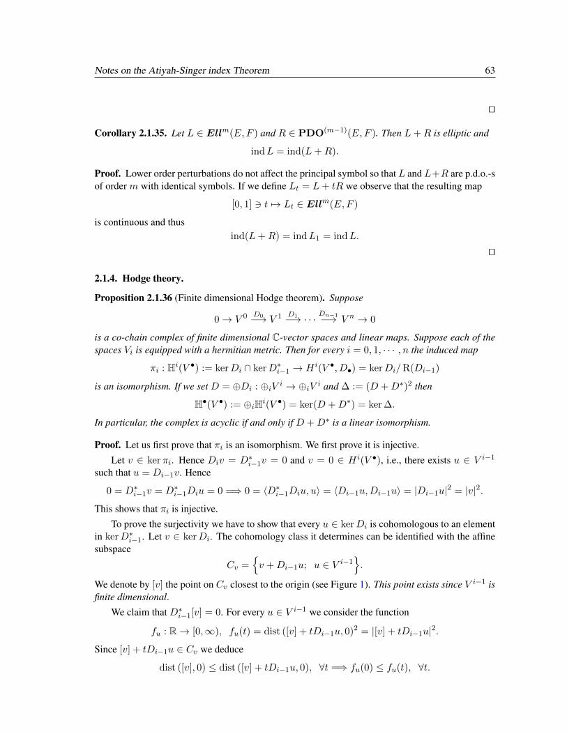
Notes on the Atiyah-Singer index Theorem 63
ut
Corollary 2.1.35. Let L ∈ Ellm(E,F ) and R ∈ PDO(m−1)(E,F ). Then L+R is elliptic and
indL = ind(L+R).
Proof. Lower order perturbations do not affect the principal symbol so that L and L+R are p.d.o.-sof order m with identical symbols. If we define Lt = L+ tR we observe that the resulting map
[0, 1] 3 t 7→ Lt ∈ Ellm(E,F )
is continuous and thusind(L+R) = indL1 = indL.
ut
2.1.4. Hodge theory.
Proposition 2.1.36 (Finite dimensional Hodge theorem). Suppose
0→ V 0 D0−→ V 1 D1−→ · · · Dn−1−→ V n → 0
is a co-chain complex of finite dimensional C-vector spaces and linear maps. Suppose each of thespaces Vi is equipped with a hermitian metric. Then for every i = 0, 1, · · · , n the induced map
πi : Hi(V •) := kerDi ∩ kerD∗i−1 → H i(V •, D•) = kerDi/R(Di−1)
is an isomorphism. If we set D = ⊕Di : ⊕iV i → ⊕iV i and ∆ := (D +D∗)2 then
H•(V •) := ⊕iHi(V •) = ker(D +D∗) = ker ∆.
In particular, the complex is acyclic if and only if D +D∗ is a linear isomorphism.
Proof. Let us first prove that πi is an isomorphism. We first prove it is injective.
Let v ∈ kerπi. Hence Div = D∗i−1v = 0 and v = 0 ∈ H i(V •), i.e., there exists u ∈ V i−1
such that u = Di−1v. Hence
0 = D∗i−1v = D∗i−1Diu = 0 =⇒ 0 = 〈D∗i−1Diu, u〉 = 〈Di−1u,Di−1u〉 = |Di−1u|2 = |v|2.
This shows that πi is injective.
To prove the surjectivity we have to show that every u ∈ kerDi is cohomologous to an elementin kerD∗i−1. Let v ∈ kerDi. The cohomology class it determines can be identified with the affinesubspace
Cv =v +Di−1u; u ∈ V i−1
.
We denote by [v] the point on Cv closest to the origin (see Figure 1). This point exists since V i−1 isfinite dimensional.
We claim that D∗i−1[v] = 0. For every u ∈ V i−1 we consider the function
fu : R→ [0,∞), fu(t) = dist ([v] + tDi−1u, 0)2 = |[v] + tDi−1u|2.
Since [v] + tDi−1u ∈ Cv we deduce
dist ([v], 0) ≤ dist ([v] + tDi−1u, 0), ∀t =⇒ fu(0) ≤ fu(t), ∀t.

64 Liviu I. Nicolaescu
O
v
vC
[v]
Figure 1. Finding the harmonic representative of a cocycle.
Hence f ′u(0) = 0, i.e.
0 =d
dt|t=0 〈[v] + tDi−1u, [v] + tDi−1u = 2 Re〈[v], Di−1u〉.
Hence0 = Re〈[v], Di−1u〉 = Re〈D∗i−1[v], u〉, ∀u ∈ V i−1.
If in the above equality we take u = D∗i−1[v] we conclude D∗i−1[v] = 0 which shows that πi is asurjection.
The equalityH•(V •) = ker(D +D∗)
is simply a reformulation of the fact that πi is an isomorphism.
If we let D = D +D∗, then ∆ = D2 and thus ker D ⊂ ker ∆. Conversely, if u ∈ ker ∆ then
0 = 〈∆u, u〉 = 〈D2u, u〉 = |Du|2
so that ker D ⊂ ker ∆. ut
Definition 2.1.37. Suppose E0, E1, . . . , EN are hermitian vector bundles over the Riemann mani-fold (M, g) and Di ∈ PDO1(Ei, Ei+1) are first order p.d.o. such that
DiDi−1 = 0, ∀i.
Then the cochain complex
0→ C∞(E0)D0−→ C∞(E1)→ · · · → C∞(EN )→ 0 (2.1.15)
is called elliptic if for any p ∈M and any ξ ∈ T ∗pM \ 0 the complex of finite dimensional spaces
0→ E0p
σp(D0)(ξ)−→ E1p → · · · → ENp → 0 (2.1.16)
is acyclic.
We setE = ⊕kEk, D = ⊕kDk : C∞(E)→ C∞(E),
D = D +D∗, ∆ = D2. ut
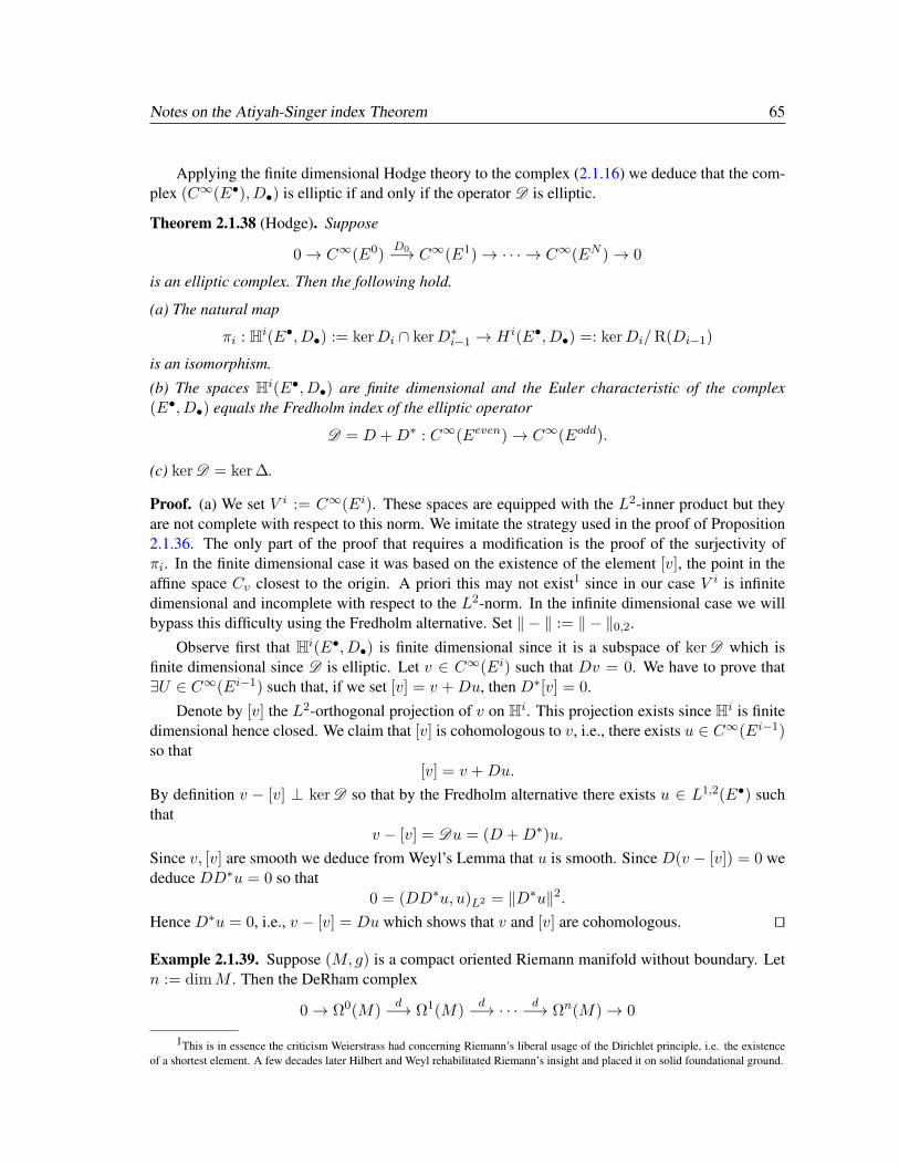
Notes on the Atiyah-Singer index Theorem 65
Applying the finite dimensional Hodge theory to the complex (2.1.16) we deduce that the com-plex (C∞(E•), D•) is elliptic if and only if the operator D is elliptic.
Theorem 2.1.38 (Hodge). Suppose
0→ C∞(E0)D0−→ C∞(E1)→ · · · → C∞(EN )→ 0
is an elliptic complex. Then the following hold.
(a) The natural map
πi : Hi(E•, D•) := kerDi ∩ kerD∗i−1 → H i(E•, D•) =: kerDi/R(Di−1)
is an isomorphism.
(b) The spaces Hi(E•, D•) are finite dimensional and the Euler characteristic of the complex(E•, D•) equals the Fredholm index of the elliptic operator
D = D +D∗ : C∞(Eeven)→ C∞(Eodd).
(c) ker D = ker ∆.
Proof. (a) We set V i := C∞(Ei). These spaces are equipped with the L2-inner product but theyare not complete with respect to this norm. We imitate the strategy used in the proof of Proposition2.1.36. The only part of the proof that requires a modification is the proof of the surjectivity ofπi. In the finite dimensional case it was based on the existence of the element [v], the point in theaffine space Cv closest to the origin. A priori this may not exist1 since in our case V i is infinitedimensional and incomplete with respect to the L2-norm. In the infinite dimensional case we willbypass this difficulty using the Fredholm alternative. Set ‖ − ‖ := ‖ − ‖0,2.
Observe first that Hi(E•, D•) is finite dimensional since it is a subspace of ker D which isfinite dimensional since D is elliptic. Let v ∈ C∞(Ei) such that Dv = 0. We have to prove that∃U ∈ C∞(Ei−1) such that, if we set [v] = v +Du, then D∗[v] = 0.
Denote by [v] the L2-orthogonal projection of v on Hi. This projection exists since Hi is finitedimensional hence closed. We claim that [v] is cohomologous to v, i.e., there exists u ∈ C∞(Ei−1)so that
[v] = v +Du.
By definition v − [v] ⊥ ker D so that by the Fredholm alternative there exists u ∈ L1,2(E•) suchthat
v − [v] = Du = (D +D∗)u.
Since v, [v] are smooth we deduce from Weyl’s Lemma that u is smooth. Since D(v − [v]) = 0 wededuce DD∗u = 0 so that
0 = (DD∗u, u)L2 = ‖D∗u‖2.Hence D∗u = 0, i.e., v − [v] = Du which shows that v and [v] are cohomologous. ut
Example 2.1.39. Suppose (M, g) is a compact oriented Riemann manifold without boundary. Letn := dimM . Then the DeRham complex
0→ Ω0(M)d−→ Ω1(M)
d−→ · · · d−→ Ωn(M)→ 0
1This is in essence the criticism Weierstrass had concerning Riemann’s liberal usage of the Dirichlet principle, i.e. the existenceof a shortest element. A few decades later Hilbert and Weyl rehabilitated Riemann’s insight and placed it on solid foundational ground.
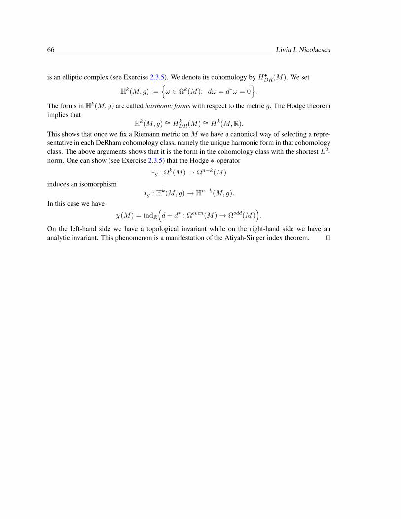
66 Liviu I. Nicolaescu
is an elliptic complex (see Exercise 2.3.5). We denote its cohomology by H•DR(M). We set
Hk(M, g) :=ω ∈ Ωk(M); dω = d∗ω = 0
.
The forms in Hk(M, g) are called harmonic forms with respect to the metric g. The Hodge theoremimplies that
Hk(M, g) ∼= HkDR(M) ∼= Hk(M,R).
This shows that once we fix a Riemann metric on M we have a canonical way of selecting a repre-sentative in each DeRham cohomology class, namely the unique harmonic form in that cohomologyclass. The above arguments shows that it is the form in the cohomology class with the shortest L2-norm. One can show (see Exercise 2.3.5) that the Hodge ∗-operator
∗g : Ωk(M)→ Ωn−k(M)
induces an isomorphism∗g : Hk(M, g)→ Hn−k(M, g).
In this case we have
χ(M) = indR
(d+ d∗ : Ωeven(M)→ Ωodd(M)
).
On the left-hand side we have a topological invariant while on the right-hand side we have ananalytic invariant. This phenomenon is a manifestation of the Atiyah-Singer index theorem. ut
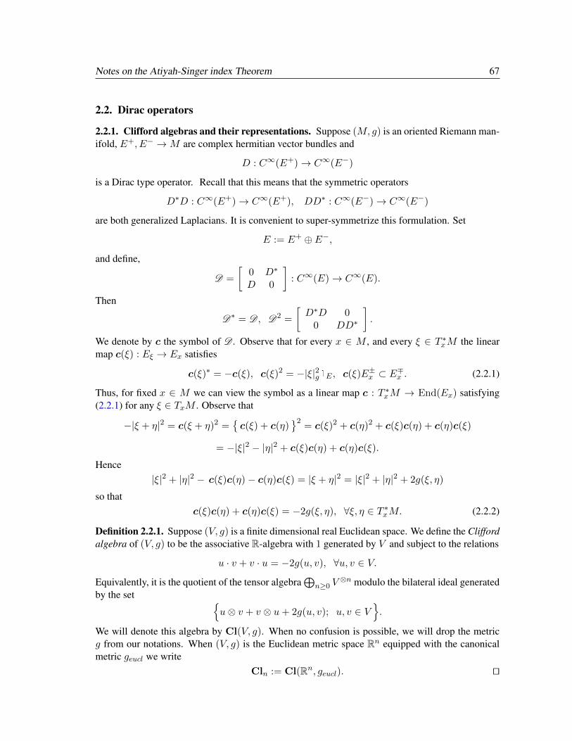
Notes on the Atiyah-Singer index Theorem 67
2.2. Dirac operators
2.2.1. Clifford algebras and their representations. Suppose (M, g) is an oriented Riemann man-ifold, E+, E− →M are complex hermitian vector bundles and
D : C∞(E+)→ C∞(E−)
is a Dirac type operator. Recall that this means that the symmetric operators
D∗D : C∞(E+)→ C∞(E+), DD∗ : C∞(E−)→ C∞(E−)
are both generalized Laplacians. It is convenient to super-symmetrize this formulation. Set
E := E+ ⊕ E−,
and define,
D =
[0 D∗
D 0
]: C∞(E)→ C∞(E).
Then
D∗ = D , D2 =
[D∗D 0
0 DD∗
].
We denote by c the symbol of D . Observe that for every x ∈ M , and every ξ ∈ T ∗xM the linearmap c(ξ) : Eξ → Ex satisfies
c(ξ)∗ = −c(ξ), c(ξ)2 = −|ξ|2g1E , c(ξ)E±x ⊂ E∓x . (2.2.1)
Thus, for fixed x ∈ M we can view the symbol as a linear map c : T ∗xM → End(Ex) satisfying(2.2.1) for any ξ ∈ TxM . Observe that
−|ξ + η|2 = c(ξ + η)2 =c(ξ) + c(η)
2= c(ξ)2 + c(η)2 + c(ξ)c(η) + c(η)c(ξ)
= −|ξ|2 − |η|2 + c(ξ)c(η) + c(η)c(ξ).
Hence|ξ|2 + |η|2 − c(ξ)c(η)− c(η)c(ξ) = |ξ + η|2 = |ξ|2 + |η|2 + 2g(ξ, η)
so thatc(ξ)c(η) + c(η)c(ξ) = −2g(ξ, η), ∀ξ, η ∈ T ∗xM. (2.2.2)
Definition 2.2.1. Suppose (V, g) is a finite dimensional real Euclidean space. We define the Cliffordalgebra of (V, g) to be the associative R-algebra with 1 generated by V and subject to the relations
u · v + v · u = −2g(u, v), ∀u, v ∈ V.
Equivalently, it is the quotient of the tensor algebra⊕
n≥0 V⊗n modulo the bilateral ideal generated
by the set u⊗ v + v ⊗ u+ 2g(u, v); u, v ∈ V
.
We will denote this algebra by Cl(V, g). When no confusion is possible, we will drop the metricg from our notations. When (V, g) is the Euclidean metric space Rn equipped with the canonicalmetric geucl we write
Cln := Cl(Rn, geucl). ut
68 Liviu I. Nicolaescu
We see that the symbol of the Dirac type operator D defines a representation of the Cliffordalgebra Cl(T ∗xM, g) on the complex Hermitian vector space Ex. We are thus forced to investigatethe representations of Clifford algebras. We need to introduce a bit of terminology.
For any elements a, b in an associative algebra A we define their anti-commutator by
a, b := ab+ ba.
A super-space (or s-space) is a vector space E equipped with a Z/2-grading, i.e., a direct sumdecomposition E = E+ ⊕ E−. The elements in E± are called even/odd.
If E = E+ ⊕ E− is a s-space and T ∈ End(E), then we say that T is even (resp. odd) if itpreserves (reap. reverses) parity, i.e.,
TE± ⊂ E± (resp. TE± ⊂ E∓).
The even endomorphisms have the diagonal form[A 00 B
]and the odd endomorphisms have the anti-diagonal form[
0 CD 0
].
We see that every endomorphism T decomposes in homogeneous components
T = Teven + Todd.
The supertrace (or s-trace) of an even endomorphism T of E is defined by
str(T ) = tr(T |E+)− tr(T |E−).
in general we setstrT := strTeven.
The grading of E is the operator
γ = γE = 1E+ ⊕−1E−[1E+ 0
0 −1E−
].
ThenstrT = tr(γT ).
A linear operator T : E0 → E1 between two s-spaces is even iff T (E±0 ) ⊂ E±1 and odd iffT (E±0 ) ⊂ E∓1 .
A super-algebra over the field K is an associative K-algebra A equipped with a Z/2-grading,i.e., a direct sum decomposition
A = A + ⊕A −
such thatA + ·A + ⊂ A +, A + ·A − ⊂ A −, A − ·A − ⊂ A +.
The elements of A ± are called even/odd, while the elements in A +∪A − are called homogeneous.For a ∈ A ± we set
sign(a) := ±1.
We see that if E is a K-vector s-space, then EndK(E) is a s-algebra. We will use the notationEndK(E) to indicate the presence of a s-structure.
Notes on the Atiyah-Singer index Theorem 69
The supercommutator on a s-algebra is the bilinear map
[−,−]s : A ×A → A
uniquely determined by the requirements
• [a±, b+]s = [a±, b+] = a±b+ − b+a±,
• [a+, b±]s = [a+, b±] = a+b± − b±a+,
• [a−, b−]s = a−, b− = a−b− + b−a−,
∀a±, b± ∈ A ± . Two elements a, b are said to super-commute if [a, b]s = 0.
If A ,B are two s-algebras, then their s-tensor product A ⊗B is defined by(A ⊗B
)+=(A + ⊗B+
)⊕(A − ⊗B−
),(
A ⊗B)−
=(A + ⊗B−
)⊕(A − ⊗B+
),
and the product is defined by
(a1 ⊗ b1) · (a1 ⊗ b2) = sign(a2) sign(b1)(a1a2)⊗ (b1b2),
for every homogeneous elements a1, a2 ∈ A , b1, b2 ∈ B.
If A = EndK(E), then str(
[S, T ]s)
= 0, so that the supertrace is uniquely determined by theinduced linear map
str : EndK(E)/[
EndK(E), EndK(E)]s→ K.
A s-module over the s-algebra A = A + ⊕A − is a K-super-space E = E+ ⊕E− together with amorphism of s-K-algebras
A → EndK(E+ ⊕ E−).
Proposition 2.2.2. Suppose that (V, g) is an n-dimensional real Euclidean vector space. ThenCl(V, g) is a s-algebra and
dimR Cl(V, g) = 2n.
Proof. Consider the isometryε : V → V, ε(v) = −v.
It induces a morphism of algebras
ε :⊕k≥0
V ⊗k →⊕k≥0
V ⊗k,
ε(v1 ⊗ · · · ⊗ vk) = ε(v1)⊗ · · · ⊗ ε(vk) = (−1)kv1 ⊗ · · · ⊗ vk.Clearly
ε(u⊗ v + v ⊗ u) = u⊗ v + v ⊗ u.Since ε is an isometry we deduce that ε induces a morphism of algebras
ε : Cl(V, g)→ Cl(V, g)
satisfying ε2 = 1. DefineCl±(V, g) := ker(±1− ε).
The decomposition Cl(V, g) = Cl+(V, g)⊕Cl−(V, g) defines a structure of s-algebra on Cl(V, g).
Now choose an orthonormal basis e1, . . . , en of V . Then in Cl(V, g) we have the equalities,
e2i = −1, eiej = −ejei, ∀i 6= j.

70 Liviu I. Nicolaescu
For every ordered multi-index I = (i1 < · · · < ik) we set
eI := ei1 . . . eik , |I| = k.
We deduce that the collection eI spans Cl(V, g) so that
dimR Cl(V, g) ≤ 2n.
To prove the reverse inequality, we define for every v ∈ V the endomorphism c(v) of Λ•V by theequality
c(v)ω =(e(v)− i(v†)
)ω,
where e(v) denotes the exterior multiplication by v and iv† denotes the contraction with the metricdual v† ∈ V ∗ of v. The Cartan formula implies
c(v)2 = −|v|2
so that we have a morphism of algebras
Cl(V, g)→ End(Λ•V ).
In particular we get a linear map
σ : Cl(V, g)→ Λ•V, Cl(V, g) 3 x 7→ c(x)1 ∈ Λ•V.
Observe thatσ(ei1 · · · eik) = c(ei1) · · · c(eik)1 = ei1 ∧ · · · ∧ eik .
Since the collection ei1 ∧ · · · ∧ eik forms a basis of Λ•V we deduce that σ is onto so that
dimR Cl(V, g) ≥ dimR Λ•V = 2n.
In particular σ is a vector space isomorphism. ut
Definition 2.2.3. The vector space isomorphism σ : Cl(V, g)→ Λ•V is called the symbol map. ut
Observe that the symbol map is an isomorphism of super-spaces. An orientation on V deter-mines a canonical element Ω on detV , the unique positively oriented element of length 1. In termsof an oriented orthonormal basis (e1, . . . , en) we have
Ω = e1 ∧ · · · ∧ en.
Using the symbol map we get an element
Γ := σ−1(Ω) = e1 · · · enwhich satisfies the identities
eiΓ = (−1)n−1Γei, Γ2 = (−1)n(n+1)/2. (2.2.3)
We would like to investigate the structure of the Z/2-graded complex Cl(V )-modules, or Cliffordmodules.
A Clifford s-module is a pair (E, c), where E is a s-space and c is an even morphism of Z/2-graded algebras
ρ : Cl(V )→ End(E).
The operationCl(V )× E → E, (x, e) 7→ c(x)e
Notes on the Atiyah-Singer index Theorem 71
is called the Clifford multiplication by x. Observe that for any v ∈ V we have
c(v)E± = E∓.
A morphism of Clifford s-modules, or Clifford morphism, between the Clifford s-modulesE0, E1 is a linear map T : E0 → E1 which supercommutes with the Clifford action. In otherwords, this means that
[T, c(x)]s = 0, ∀x ∈ Cl(V ).
We denote by HomCl(V )(E0, E1) the space of Clifford morphisms and by EndCl(V )(E) the s-algebra of Clifford endomorphisms of the Clifford module E.
Since we will be interested only in complex representations of Cl(V, g) we will study only thestructure of the complexified Clifford algebra
Cl(V, g) := Cl(V, g)⊗R C.
Set Vc := V ⊗R C. The metric g on V extends by complex linearity to a C- bilinear map
gc : Vc × Vc → C
Proposition 2.2.4. Assume that n = dimR V = 2m. There exists Z/2-graded Cl(V )-module SVsuch that the induced morphism of s-algebras
Cl(V )→ End(SV ),
is an isomorphism. This module is unique up to a Clifford isomorphism. Moreover, if we writeSV = S+
V ⊕ S−V , thendimC S+
V = dimC S−V = 2m−1.
Proof. Existence. Fix a complex structure on V , i.e., a skew-symmetric linear map J : V → Vsuch that J2 = −1. We can find an orthonormal basis e1, f1, . . . , em, fm of V such that
Jei = fi, Jfi = −ei, ∀i = 1, . . . ,m.
The operator J extends to the complexification Vc and since J2 = −1 we deduce that the eigen-values of J on Vc are ±i. Denote by V 1,0 the i-eigenspace of J and by V 0,1 the −i-eigenspace sothat
Vc = V 1,0 ⊕ V 0,1.
Note that Vc is equipped with an involution
w = v ⊗ z 7→ w = v ⊗ zand V 1,0 = V 0,1. Set
εj =1√2
(ej − ifj) ∈ V 1,0, εj =1√2
(ej + ifj) ∈ V 0,1.
The collection (εj) is a C-basis of V 1,0. Note that
gc(εi, εj) = gc(εj , εi) = δij , gc(εi, εj) = gc(εi, εj) = 0,
ej =1√2
(εj + εj), fi =i√2
(εj − εj). (2.2.4)
DefineSV := Λ•V 1,0. (2.2.5)
72 Liviu I. Nicolaescu
We want to produce a representation of Cl(V ) on SV , that is, a C-linear map
c : Vc → EndC(SV )
such thatc(v)2 = −gc(v, v), ∀v ∈ Vc.
Since Vc = V 1,0 ⊕ V 0,1 it suffices to describe how the elements in V 1,0 and the elements of V 0,1
act on Sn.
For every w ∈ V 1,0 we setc(w) :=
√2e(w),
where e(w) denotes the exterior multiplication by w on Λ•V 1,0. For every w ∈ V 1,0 we havew = V 0,1 and define the contraction
i(w) = w : Λ•V 1,0 → Λ•−1V 1,0
byw (w1 ∧ · · · ∧ wk) = gc(w, w1)w2 ∧ · · · ∧ wk − gc(w, w2)w1 ∧ w3 ∧ · · · ∧ wk
+ · · ·+ (−1)k−1gc(w, wk)w1 ∧ · · · ∧ wk−1.
Now setc(w) := −
√2w .
For any w0, w1 ∈ V 1,0 we have the equalities2
c(w)2 = c(w)2 = 0, c(w0 + w1)2 = c(w0)c(w1) + c(w1)c(w0), (2.2.6a)
gc(w0 + w1, w0 + w1) = 2gc(w0, w1), (2.2.6b)c(w0)c(w1) + c(w1)c(w0) = −2gc(w0, w1). (2.2.6c)
Hence the map c : Vc → EndC(Λ•V 1,0) extends to a morphism of algebras
c : Cl(V )→ EndC(Λ•V 1,0).
The space Λ•V 1,0 is Z/2-graded
Λ•V 1,0 = ΛevenV 1,0 ⊕ ΛoddV 1,0
and clearly c maps even/odd elements of Cl(V ) to even/odd elements of EndC(Λ•V 1,0). Note thatfor any 1 ≤ i1 < · · · < ik ≤ m we have
c(εi1εi2 · · · εik)1 = 2k/2εi1 ∧ εi2 ∧ · · · ∧ εik ,c(εi1εi2 · · · εik)ε1 ∧ · · · ∧ εm = 0, c(εi1 εi2 · · · εik)1 = 0,
c(εi1 εi2 · · · εik)ε1 ∧ · · · ∧ εm = (−1)k+∑ks=1(is−s)2
k2 εj1 ∧ · · · ∧ εjm−k ,
wherej1 < · · · < jm−k, 1, . . . ,m = i1, . . . , im ∪ j1, . . . , jm−k.
This prove that for any u ∈ ClC(V ) \ 0 we have
c(u)(1 + ε1 ∧ · · · ∧ εn) 6= 0.
Hence the map c : Cl(V )→ EndC(Λ•V 1,0) is injective. Now observe that
dimC EndC(Λ•V 1,0) =(dimC Λ•V 1,0)2 = (2dimC V
1,0)2 = 22m = 2n = dimCCl(V ),
2 Only (2.2.6c) is nontrivial. Because the two sides of (2.2.6c) are C-bilinear in (w0, w1) it suffices to verify it only in the specialcase w0 = εj , w1 = εk for some j, k.

Notes on the Atiyah-Singer index Theorem 73
which shows that c is an isomorphism.
The uniqueness of the module SV follows from Schur’s Lemma, [16, Chap. XVII, Prop. 1.1].ut
Definition 2.2.5. Assume dimV is even. The complex Clifford s-module SV constructed in Propo-sition 2.2.4 is called the space of complex spinors. The corresponding representation
c : Cl(V )→ End(SV )
is called the complex spinorial representation. ut
We have shown that, if we forget the grading, the Clifford algebra Cl2m is isomorphic to analgebra of matrices, End(S2m) and the representations of such an algebra are well understood. Letus describe a simple procedure of constructing Z/2-graded complex representations of Cl2m.
SupposeW = W+⊕W− is a complex s-space. Denote by SV ⊗W the s-vector space S2m⊗Wequipped with the Z/2-grading
(SV ⊗W )+ = S+V ⊗W
+ ⊕ S−V ⊗W−, (SV ⊗W )− = S+
V ⊗W− ⊕ S−V ⊗W
+.
We define the complex spinorial representation twisted by W to be
cW : Cl(V )→ EndC(SV ⊗W ),
cW (x)(ψ ⊗ w) = (c(x)ψ)⊗ w, ∀ψ ∈ SV , w ∈W.Observe that each w ∈W defines a morphism of Cl(V )-modules
TW (w) : SV → SV ⊗W, ψ 7→ ψ ⊗ wand thus we get a linear map
TW : W → HomCl(V )(SV ,SV ⊗W ).
Similarly every linear map Φ : W →W defines a morphism of Cl(V )-modules
SΦ : SV ⊗W → SV ⊗W, ψ ⊗ w 7→ ψ ⊗ Φ(w).
We obtain in this fashion a linear map
S : EndC(W )→ EndCl(V )(SV ⊗W, SV ⊗W ),
cW ⊗S : Cl(V )⊗EndC(W )→ EndC(SV ⊗W ).
The representation theory of algebras (see [16, Chap. XVII] or [33, Chap. 14]) imply that thesemaps are isomorphisms. We gather all the above observations in the following result.
Proposition 2.2.6. Suppose E is a Z/2-graded Cl(V )-module, dimR V = 2m. Then E is isomor-phic as a Z/2-graded Cl(V )-modules with the complex spinorial module twisted by the s-space
W = HomCl(SV , E).
Moreover, we have an isomorphism of s-algebras
Cl(V )⊗EndC(W )→ EndC(E). (2.2.7)
Via this isomorphism, we can identify EndC(W ) with the subalgebra of EndC(E) consisting ofendomorphism T : E → E commuting with the Clifford action. In other words
EndC(W ) ∼= EndCl(V )(E), Cl(V )⊗EndCl(V )(E) ∼= EndC(E). (2.2.8)
74 Liviu I. Nicolaescu
ut
The s-space HomCl(SV , E) is called the twisting space of the Clifford module E and will bedenoted by E/S. We deduce from the above result that given a Clifford module E we can identifya Clifford endomorphism L : E → E with a linear map L/S on the twisting space E/S, i.e.
EndCl(V )(E) ∼= EndC(E/S), L 7→ L/S.
Definition 2.2.7. The relative supertrace of an endomorphism L ∈ EndCl(V )(E) of a Z/2-gradedcomplex Cl2m-module E is the scalar strE/S L defined as the supertrace of the linear operator L/S,
strE/S L := strL/S. ut
Suppose that E is a Z/2-graded Cl(V )-module so that we can represent it as a twist of SV withan s-space W . We would like to relate the relative supertrace
strE/S : EndC(W )→ C.
to the absolute supertracestrE : EndC(E)→ C.
Suppose F : E → E is a linear map. By choosing a basis of W we can represent it as a matrixwith coefficients in Cl(V ). Equivalently, we can regard F as an element of Cl(V )⊗End(W ) =
End(SV )⊗End(W ) and we can write
F =∑`
u` ⊗ F`, u` ∈ End(SV ), F` ∈ End(W ).
We would like to compute str(F : E → E). By linearity we have
str(F ) =∑`
str(u` ⊗ F`).
Choose orthonormal bases w±i in W± and orthonormal bases ψ±j in S±V . Define a metric on Cl(V )
by declaring the basis (eI) orthonormal. Then⟨(u` ⊗ F`)(ψ±i ⊗ w
±j ), ψ±i ⊗ w
±j
⟩=⟨u`ψ
±i , ψ
±i 〉〈F`w
±j , w
±j
⟩.
It follows from this equality that
str(u` ⊗ F` ) = str(u` : SV → SV
)· str(F` : W →W ).
Thus we need to compute the supertrace of the action of an element in the Clifford algebra on thecomplex spinorial space. This supertrace is uniquely determined by the induced linear map
Cl(V )/[Cl(V ),Cl(V )]s = End(SV )/[End(SV ), End(SV )]s → C.
It turns out that the space Cl(V )/[Cl(V ),Cl(V )]s is quite small.
Choose an orthonormal basis (ei) of V . Fix 1 ≤ r ≤ n = dimV . Observe that for everymulti-index I = (1 ≤ i1 < · · · < ik−1 ≤ n), ij 6= r, we have
[er, ereI ]s = e2reI − (−1)kereIer = 2e2
reI = −2eI ⇐⇒ eI =[er,−
1
2ereI
]s
Notes on the Atiyah-Singer index Theorem 75
This shows that any monomial eI , |I| < dimV is a s-commutator. Hence the only monomial eIthat could have nontrivial s-trace must be Γ = e1 · · · e2m.
To compute the s-trace of Γ as a linear map on SV we choose a complex structure J on V andan orthonormal basis e1, f1, . . . , em, fm such that
fi = Jei, ei = −Jfi.
Consider as before
εj =1√2
(ej − ifj) ∈ V 1,0, εj =1√2
(ej + ifj) ∈ V 0,1.
Then,
ei =1√2
(εi + εi), fi =i√2
(εi − εi),
c(ej) = e(εj)− εj , c(fj) = i(e(εj) + εj
),
and
Γ =
m∏j=1
c(ej)c(fj) = imm∏j=1
(e(εj)− εj
)(e(εj) + i(εj)
)= im
m∏s=1
(e(εj)εj −(εj )e(εj)
).
For a multi-index J = j1 < · · · < jk we set
εJ = εj1 ∧ · · · ∧ εjk ∈ ΛkV 1,0
and we have
e(εj)(εj )εJ =
εJ if j ∈ J0 if j 6∈ J , (εj )e(εj)εJ =
εJ if j 6∈ J0 if j ∈ J.
Putting these two facts together we deduce(e(εj)(εj )− (εj )e(εj)
)εJ =
εJ if j ∈ J−εJ if j 6∈ J.
HenceΓεJ = im(−1)m−|J |︸ ︷︷ ︸
:=〈εJ |Γ|εJ 〉
εJ ,
and thus
str Γ =∑J
(−1)|J |〈εJ |Γ|εJ〉 =∑J
(−1)|J |im(−1)m−|J | = (−i)m∑J
1 = (−2i)m.
Let us summarize what we have proved so far.
Assume V is oriented. The orientation and the metric g determine a canonical section of detV ,the volume form Ωg. For every ω ∈ Λ•V ⊗C we denote by [ω]k ∈ ΛkV ⊗C its degree k component.We then define 〈ω〉 ∈ C by the equality
[ω]n = 〈ω〉Ωg.
We have thus established the following result.

76 Liviu I. Nicolaescu
Proposition 2.2.8. Assume that V is an oriented Euclidean space of dimension dimV = 2m. Ifu ∈ Cl(V ), W is a s-space and F ∈ End(W ), then
str(u⊗ F : SV ⊗W → SV ⊗W
)= (−2i)m
⟨σ(u)
⟩strF.
In the above equality, both sides depend on a choice of an orientation on V . ut
If in the above equality we choose u = Γ, we observe that 〈σ(Γ)〉 = 1, and we deduce thefollowing useful consequence.
Corollary 2.2.9. Suppose (V, g) is oriented and dimR V = 2m. Then for any Clifford module Eand any endomorphism of Clifford modules L : E → E we have
strE/S L =im
2mstrE
(ΓL),
where in the right-hand-side of the above equality we regard ΓL : E → E as a morphism ofC-vector spaces. ut
Remark 2.2.10. Let us say a few words about the odd dimensional case. If V is an odd dimensionalvector space and U := R⊕ V , then we have a natural isomorphism of algebras
Cl(V )→ Cleven(U), Cleven(V )⊕Clodd(V ) 3 x0 ⊕ x1 7→ x0 + e0x1,
where e0 denotes the canonical basic vector of the summand R of U . We can then prove that wehave an isomorphism of algebras
Cl(V ) ∼= End(S+U )⊕ EndC(S−U ).
For more details we refer to [17]. ut
2.2.2. Spin and Spinc. Suppose that (V, g) is a finite dimensional Euclidean space. Recall thatwe have a vector space isomorphism
σ : Cl(V )→ Λ•V
called the symbol map. Its inverse is called the quantization map and it is denote by q. Set
spin(V ) := q(Λ2V ) ⊂ Cl(V ).
If e1, . . . , en is an orthonormal basis of V , then eiej ; 1 ≤ i < j ≤ n is a basis of spin(V ).Observe that
[eiej , ek] = eiejek − ekeiek = ei(−2δjk − ekej)− ekeiek= −2δjkei − (−2δik − ekei)ej − ekeiek = −2δjkei + 2δikej .
Hence[ω, v] ∈ V, ∀ω ∈ spin(V ), v ∈ V.
Using the identity[eiej , ejek] = [eiek, ek]e` + ej [eiej , e`]
we deduce[eiej , eke`] ∈ spin(V ), ∀i < j, k < `,
which shows that spin(V ) is a Lie algebra with respect to the commutator in Cl(V ).
Notes on the Atiyah-Singer index Theorem 77
The Jacobi identity shows that we have a morphism of Lie algebras
τ : spin(V )→ End(V ), τ(η)v = [η, v]. (2.2.9)
Observe thatg(τ(eiej)ek, e`) = −g(ek, τ(eiej)e`)
so that τ(η) is skew symmetric ∀η ∈ spin(V ), i.e., τ(η) ∈ so(V ). Note that
τ(eiej) = 2Xij ,
where for i < j we denoted by Xij the operator V → V defined by
Xijei = ej , Xijej = −ei, Xijek = 0, ∀k 6= i, j.
This implies that τ is injective. On the other hand
dimR spin(V ) = dimR Λ2V = dimR so(V ),
so that τ is an isomorphism.
To every A ∈ so(V ) we associate ωA ∈ Λ2V
ωA =∑i<j
g(Aei, ej)ei ∧ ej .
Observe thatA =
∑i<j
g(Aei, ej)Xij .
Indeed ∑i<j
g(Aei, ej)Xijek =∑i<k
g(Aei, ek)Xikek +∑j>k
g(Aek, ej)Xkjek
= −∑i<k
g(Aei, ek)ei +∑j>k
g(Aek, ej) =∑i
g(ei, Aek)ei = Aek.
Hence
τ−1(A) =∑i<j
g(Aei, ej)τ−1(Xij) =
1
2
∑i<j
g(Aei, ej)eiej =1
2q(ωA). (2.2.10)
Definition 2.2.11. For any euclidean space (V, g) we denote by Spin(V, g) the group
Spin(V, g) :=u ∈ Cleven(V ); u = v1 · · · v2k, vi ∈ V, |vi|g = 1
.
In particular, we setSpin(n) := Spin(Rn). ut
Observe that for any u ∈ Spin(V, g) we have
uV u−1 ⊂ V,
so that we have a natural map
ρ : Spin(V, g)→ Aut(V ), ρ(u)v = uvu−1.
For any u, v ∈ V , |u|g = 1 we have
−uvu−1 = uvu = u(−2g(u, v)− uv
)= v − 2g(u, v)u ∈ V.

78 Liviu I. Nicolaescu
Hence the map V → V , v 7→ −uvu−1 is described by the orthogonal reflection Ru in the hyper-plane through the origin orthogonal to u. In particular, it is an orthogonal transformation of V withdeterminant −1. Thus if u = u1 · · ·u2k the ρu is the product of an even number of reflections
ρ(u) = Ru1 · · ·Ru2k
so that we have a well defined morphism
ρ : Spin(V, g)→ SO(V, g).
Lemma 2.2.12. The morphism ρ is surjective and
ker ρ ∼= ±1 ⊂ Spin(V ).
Proof. The surjectivity follows from the classical fact that any orthogonal transformation is a prod-uct of reflections. If η ∈ ker ρ then
ηv = vη, ∀v ∈ V
from which we conclude that u lies in the center of Cl(V ).
Choose an orthonormal basis e1, . . . , en of V so we can write
η =∑I
ηIeI , uI ∈ R,
and the sum is carried over all even dimensional ordered multi-indices I . Since η commutes withek, the multi-indices I such that ηI 6= 0 cannot contain k. Since this happens for all k the abovesum should contain only the empty multiindex for which e∅ = 1. Hence η must be a scalar, η ∈ R.
To show that |η| = 1 we consider the representation
c : Cl(V )→ End(Λ•V ).
The metric on V induces a metric on Λ•V and thus for every u ∈ Cl(V ) the linear map
c(u) : Λ•V → Λ•V
has a well defined norm ‖c(u)‖. Moreover
‖c(u1u2)‖ ≤ ‖c(u1)‖ · ‖c(u2)‖.
Observe that if v ∈ V is a vector of length one, then ‖c(v)‖ = 1. We deduce that ‖c(u)‖ ≤ 1 forall u ∈ Spin(V ). In particular η, η−1 ∈ Spin(V ) ∩ R and we deduce
|η| = ‖c(η)‖ ≤ 1, |η−1| = ‖c(η−1)‖ ≤ 1.
Hence |η| = 1. This completes the proof. ut
We have produced a 2 : 1 group morphism
ρ : Spin(V, g)→ SO(V, g).
We want to prove that Spin(V, g) with the topology induced as a subset of Cl(V, g) equipped withthe above norm is a topological group and the above map is a topological covering map. We beginwith a few simple observations.
Let v, w ∈ V , v ⊥ w, |v| = |w| = 1. Then
(vw)2 = −1,

Notes on the Atiyah-Singer index Theorem 79
and thusexp(tvw) = cos t+ (sin t)vw ∈ Cl(V, g).
Note that exp(tvw) ∈ Spin(V, g), ∀t ∈ R. Indeed, we have
cos t+ (sin t)uw =(
(sin t/2)u− (cos t/2)w)(
(sin t/2)u+ (cos t/2)w), (2.2.11)
and ∣∣ (sin t/2)u− (cos t/2)w∣∣ =
∣∣ (sin t/2)u+ (cos t/2)w∣∣ = 1.
We denote by Xvw the skew-symmetric endomorphism of V defined by
Xvwu =
w, u = v,
−v, u− w,0, u ⊥ v, w
Lemma 2.2.13. For any v, w ∈ V such that v ⊥ w, |v| = |w| = 1 we have
ρ(
exp(tvw))u = exp(tvw)u exp(−tvw) = exp(2tXvw)u
Proof. If u ⊥ v, w, then u commutes with exp(tvw) so that
ρ(
exp(tvw))u = exp(tvw)u exp(−tvw) = u = exp(2tXvw)u.
Next,ρ(
exp(tvw))v =
(cos t+ (sin t)vw
)v(
cos t− (sin t)vw)
=(
(cos t)v − (sin t)w)(
cos t− (sin t)vw)
= (cos 2t)v + (sin 2t)w = exp(2tXvw)v.
Similarlyρ(
exp(tvw))w = −(sin 2t)v + (cos 2t)w = exp(2tXvw)w.
ut
Proposition 2.2.14. Let (V, g) be an Euclidean space of dimension n. Set
m :=⌊n
2
⌋.
Then for any u ∈ Spin(V, g) we can find an orthonormal system of vectors
v1, w1, . . . , vm, wm ∈ V
and real numbers t1, . . . , tm such that
u = exp(t1v1w1) · · · exp(tmvmwm) = exp(t1u1v1 + . . .+ tmvmwm).
Proof. Let T = ρ(u) ∈ SO(V, g). We can then find A ∈ so(V, g) and t ∈ R such that
T = exp(2tA).
The spectral theory of skew-symmetric matrices shows that we can find an orthonormal systemv1, w1, . . . , vm, wm and real numbers λ1, . . . , λm such that
A =∑j
λjXvjwj .

80 Liviu I. Nicolaescu
Note that the matrices Xv1w1 , . . . , Xvmwm pairwise commute to that
exp(2tA) =
m∏j=1
exp(2tλjXvjwj ).
We set
u′ :=m∏j=1
exp(tλjvjwj),
and we deduce from Lemma 2.2.13 that
ρ(u′) = exp(2tA) = ρ(u).
Hence u′ = ±u. If u′ = u the claim is proved with tj = tλj . Othervise we observe that
u = −u′ = exp(
(tλ1 + π)v1w1
) m∏j=2
exp(2tλjXvjwj ).
ut
We have the following corollary of the above proof
Corollary 2.2.15. For any A ∈ so(V, g) we have
ρ(
exp τ−1(A))
= exp(A). ut
Corollary 2.2.16. Spin(V, g) is a compact subset of Cl(V, g).
Proof. Using Lemma 2.2.13 and the equality (2.2.11) we deduce that any u can be written non-uniquely as a product
u = u1u2 · · ·u2m,
where all the factors uj live of the unit sphere of (V, g). If uν is a sequence of elements in Spin(V, g)
uν = uν1uν2 · · ·uν2m,
then upon extracting a subsequence, we can assume that uνj → u∞j as ν →∞. Clearly
uν → u∞ = u∞1 u∞2 · · ·u∞2m ∈ Spin(V, g).
ut
Clearly the group Spin(V, g) with the topology induced by the norm topology on Cl(V, g)is a topological group as a subgroup of the topological group Cl(V, g)∗ of invertible elements ofCl(V, g).
Proposition 2.2.17. The morphism ρ : Spin(V, g) → SO(V, g) is a continuous group morphismand the resulting map is a topological covering map.
Proof. We have to show that if (uν) is a sequence in Spin(V, g) that converges to u∞ ∈ Spin(V, g),then ρuν → ρu∞ .
First let us write uν as a product
uν = uν1uν2 · · ·uν2m, m =
⌊n2
⌋, n = dimV, |uνj | = 1.
Notes on the Atiyah-Singer index Theorem 81
Let T ∈ SO(V, g) be a limit point of the sequence ρ(uν). We can find a subsequence (uµ) of (uν)such that
limµ→∞
uµj = u∞j , ∀j = 1, . . . , 2m,
and
T = limµ→∞
ρ(uµ) = limµ→∞
2m∏j=1
Ruµj =2m∏j=1
Ru∞j = ρ(u∞).
Hence, the only limit point of ρ(uν) is ρ(u∞).
Let us now prove that the map ρ : Spin(V, g)→ SO(V, g) is a covering map.
SetO :=
u ∈ Spin(V, g); ‖1− c(u)‖ < 1
.
Observe that O ∩ −O = ∅. Indeed, if u ∈ O ∩ (−O), then u,−u ∈ O and
2 = ‖1− (−1)‖ ≤ ‖1− c(u)‖+ ‖c(u)− (−1)‖ = ‖1− c(u)‖+ ‖c(−u)− 1‖ < 2.
SetO := ρ(O) = ρ(O ∪ −O).
By construction
SO(V, g) \ O = ρ(Spin(V, g) \
(O ∪ −O
) ),
and we deduce that SO(V, g) \ O is compact as image of a compact set. Hence O is an openneighborhood of 1 ∈ SO(V, g).
The same argument shows that the restriction of ρ to O is an open map and thus it induces ahomeomorphism O→ O.
More generally, if u ∈ Spin(V, g), u := ρ(u), then
ρ−1(uO)
= uO ∪ −uO
and the resulting map ρ : uO→ uO is a homeomorphism. ut
Corollary 2.2.18. The group Spin(V, g) is a natural Lie group structure such that
ρ : Spin(v, g)→ SO(V, g)
is a smooth group morphism. The tangent space T1Spin(V, g) is naturally identified with spin(V, g),and under this identification, the differential ρ∗ of ρ at 1 ∈ Spin(V, g) coincides with the map τ of(2.2.9).
Proof. Since the map ρ : Spin(V, g) → SO(V, g) is a 2 : 1 covering map, we can use it to lift thesmooth structure on SO(V, g) to a smooth structure on Spin(V, g). By construction, ρ is a smoothmap between these smooth structure. The fact that the group operations on Spin(V, g) are smooth,follows from the fax that ρ is a local diffeomorphism. Finally, the equality ρ∗ = τ follows fromCorollary 2.2.15. ut
Proposition 2.2.19. The group Spin(V, g) is connected if dimV > 1 and simply connected ifdimV > 2.
82 Liviu I. Nicolaescu
Proof. Suppose dimV ≥ 2. We know that every element u ∈ Spin(V, g) can be written as aproduct
u = exp(t1u1w1) · · · exp(tkukwk), |ui| = |wi| = 1, ui ⊥ wi, ti ∈ R,and thus x lies in the same path component of Spin(V, g) as 1.
Suppose dimV ≥ 3. Consider first the case dimV = 3. Fix an orthonormal basis e1, e2, e3
and setf1 = e2e3, f2 = e3e1, f3 = e1e2.
Thenf2i = −1, fifj = −fjfi, i 6= j,
f1f2 = f3, f2f3 = f1, f3f1 = f2.
We deduce thatCleven3
∼= H = the division ring of quaternions.We want to prove that Spin(3) can be identified with the group of quaternions of norm 1. Supposethat
q = a+ x, x = bf1 + cf2 + df3 6= 0, a2 + b2 + c2 + d2 = 1.
Then we can writeq = cos θ + sin θy, y =
1
|x|x.
and thusq = exp(θy), θy ∈ spin(V ).
Hence every quaternion of norm 1 can be written as the exponential of an element in spin(V ). Wecan now see that every z ∈ spin(V ) can be written as a product
z = uv, u, v ∈ V, u, v ∈ V \ 0, u ⊥ v.
More precisely, if z = af1 + bf2 + cf3, then we choose u, v such that u ⊥ v and
u× v = ae1 + be2 + ce3 ∈ V,
where × denotes the cross product. Hence every unit quaternion can be written as an exponentialexp(uv) where u, v are two nonzero orthogonal vectors in V . As we have seen before any suchelement belongs to Spin(3). Hence Spin(3) contains the group of unit quaternions.
Conversely, every element in Spin(3) can be written as a product of exponentials exp(tuv)as above, i.e., as a product of unit quaternions. Hence Spin(3) is contained in the group of unitquaternions.
This proves our claim and shows that Spin(3) is simply connected. From the 2 : 1 nontrivialcover Spin(3)→ SO(3) we deduce that SO(3) ∼= RP3 and π1(SO(3)) ∼= Z/2.
Using the homotopy long exact sequence of the fibration SO(n) → SO(n + 1) Sn, n ≥ 3we obtain the exact sequence
0 = π2(Sn)→ π1(SO(n))→ π1(SO(n+ 1))→ π1(Sn) = 0.
We deduce inductively that
π1(SO(n)) ∼= π1(SO(3)) ∼= Z/2, ∀n ≥ 3.
This implies that the covering Spin(n) → SO(n) is the universal covering of SO(n), and inparticular Spin(n) is simply connected. ut
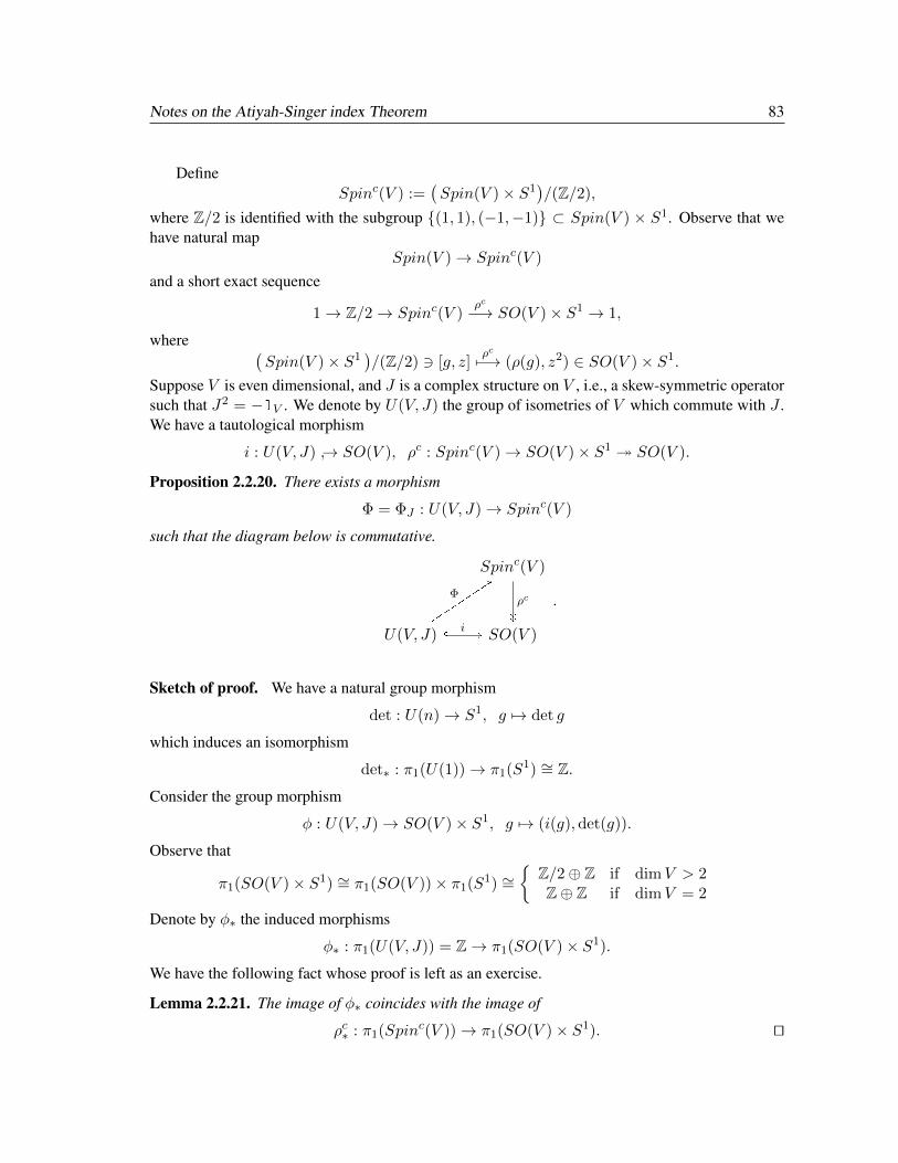
Notes on the Atiyah-Singer index Theorem 83
DefineSpinc(V ) :=
(Spin(V )× S1
)/(Z/2),
where Z/2 is identified with the subgroup (1, 1), (−1,−1) ⊂ Spin(V ) × S1. Observe that wehave natural map
Spin(V )→ Spinc(V )
and a short exact sequence
1→ Z/2→ Spinc(V )ρc−→ SO(V )× S1 → 1,
where (Spin(V )× S1
)/(Z/2) 3 [g, z]
ρc7−→ (ρ(g), z2) ∈ SO(V )× S1.
Suppose V is even dimensional, and J is a complex structure on V , i.e., a skew-symmetric operatorsuch that J2 = −1V . We denote by U(V, J) the group of isometries of V which commute with J .We have a tautological morphism
i : U(V, J) → SO(V ), ρc : Spinc(V )→ SO(V )× S1 SO(V ).
Proposition 2.2.20. There exists a morphism
Φ = ΦJ : U(V, J)→ Spinc(V )
such that the diagram below is commutative.
Spinc(V )
U(V, J) SO(V )uuρc
\\\\\]Φ
y wi
.
Sketch of proof. We have a natural group morphism
det : U(n)→ S1, g 7→ det g
which induces an isomorphism
det∗ : π1(U(1))→ π1(S1) ∼= Z.
Consider the group morphism
φ : U(V, J)→ SO(V )× S1, g 7→ (i(g),det(g)).
Observe that
π1(SO(V )× S1) ∼= π1(SO(V ))× π1(S1) ∼=
Z/2⊕ Z if dimV > 2Z⊕ Z if dimV = 2
Denote by φ∗ the induced morphisms
φ∗ : π1(U(V, J)) = Z→ π1(SO(V )× S1).
We have the following fact whose proof is left as an exercise.
Lemma 2.2.21. The image of φ∗ coincides with the image of
ρc∗ : π1(Spinc(V ))→ π1(SO(V )× S1). ut
84 Liviu I. Nicolaescu
The above lemma implies that φ admits a unique lift Φ : U(V, J) → Spinc(V ) such thatΦ(1) = [1,1]. This is the morphism with the required properties.
ut
2.2.3. Geometric Dirac operators. Suppose that (M, g) is an oriented, n-dimensional Riemannmanifold. We denote by Cl(M) the bundle over M whose fiber over x ∈M is the Clifford algebraCl(T ∗xM, g).
To construct it, we first produce the principal SO(n)-bundle PM of oriented, orthonormalframes of T ∗M . Then observe that there is a canonical morphism
ρ : SO(n)→ Aut(Cln) = the group of automorphism of the Clifford algebra Cln.
ThenCl(M) = PM ×ρ Cln .
We will refer to Cl(M) as the Clifford bundle of (M, g). Note that we have a Clifford multiplication
· : Cl(M)⊕Cl(M)→ Cl(M),
and a canonical inclusionT ∗M → Cl(M).
The symbol mapCl(V )→ Λ•V
induces an isomorphism of vector bundles
σ : Cl(M)→ Λ•T ∗M.
Definition 2.2.22. Let (M, g) be an oriented Riemann manifold.
(a) An s-bundle over M is a vector bundle E →M together with a direct sum decomposition
E = E+ ⊕ E−.
The grading of the s-bundle E is the endomorphism γ = 1E+ ⊕ (−1E−).
(b) A Clifford bundle (or Cl(M)-module) is a hermitian s-bundle together with a morphism
c : Cl(M)→ End(E)
which on each fiber is a morphism of s-algebras and for every x ∈ M , α ∈ T ∗xM ⊂ Cl(M)x theendomorphism
c(α) : Ex → Ex
is (odd) and skew-symmetric. We will refer to c(−) as the Clifford multiplication.
(c) A Dirac bundle over M is a pair (E,∇E), where E = E+⊕E− is a Clifford bundle and∇E isa hermitian connection on E which preserves the Z/2 grading and it is compatible with the Cliffordmultiplication, i.e., ∀X ∈ Vect(M), ∀α ∈ Ω1(M), ∀u ∈ C∞(E) we have
∇EX(c(α)u) = c(∇gXα)u+ c(α)∇EXu,
where∇g denotes the Levi-Civita connection on T ∗M . ut
Notes on the Atiyah-Singer index Theorem 85
Suppose (E,∇E) is a Dirac bundle. Then F∇ ∈ Ω2(EndE). Using the isomorphism ofcomplex vector bundles
EndC(E) ∼= Cl(M)⊗EndCl(M)(E).
we view the curvature of∇E as a section of
F∇ ∈ Ω2(Cl(M)⊗EndCl(M)(E)
).
On the other hand, the curvature R of the Levi-Civita connection is a section
R ∈ Ω2(so(TM)
),
where so(TM) denotes the space of skew-symmetric endomorphisms of TM . Thus, for anyX,Y ∈ Vect(M) the endomorphismR(X,Y ) of TM is skew-symmetric. We denote byR(X,Y )†
the dual, skew-symmetric endomorphism of T ∗M .
We have a map
δ : so(TM)†−→ so(T ∗M)
τ−1
−→ Cl(M),
where † : TM → T ∗M denotes the metric duality isomorphism. Via this isomorphism we canidentify the curvature R with a section
c(R) ∈ Ω2(Cl(M)
)⊂ Ω2
(Cl(M)⊗EndCl(M)(E)
).
If we choose a local orthonormal frame (ei) of TM and we denote by (ei) the dual coframe, then
R =∑i<j
R(ei, ej)ei ∧ ej , R(ei, ej) ∈ Γ
(so(TM)
),
and the equality (2.2.10) implies that
c(R)(ei, ej) =1
2
∑k<`
g(R(ei, ej)ek, el
)c(ek)c(e`)
=1
4
∑k,`
g(R(ei, ej)ek, e`
)c(ek)c(e`).
(2.2.12)
We setFE/S := F − c(R) ∈ Ω2
(Cl(M)⊗EndCl(M)(E)
).
We will refer to FE/S as the twisting curvature of the Dirac bundle (E,∇E).
Proposition 2.2.23.FE/S ∈ Ω2
(EndCl(M)(E)
).
Proof. We have to show that ∀X,Y ∈ Vect(M), ∀α ∈ Ω1(M) we have
FE/S(X,Y )c(α) = c(α)FE/S(X,Y ),
i.e., [FE/S(X,Y ), c(α)
]= 0
so that FE/S(X,Y ) is a morphism of Cl(M)-modules. We have
F∇(X,Y ) = [∇EX ,∇EY ]−∇E[X,Y ],
and [∇EZ , c(α)
]= c(∇gZα), ∀Z ∈ Vect(M).
86 Liviu I. Nicolaescu
Hence [∇E[X,Y ], c(α)
]= c(∇g[X,Y ]α),[
[∇EX ,∇EY ], c(α)]
=[
[∇EX , c(α)],∇EY]
+[∇EX , [∇EY , c(α)]
]= [c(∇gXα),∇EY ] + [∇EX , c(∇gY α)] = c
([∇gX ,∇
gY ]α
).
We deduce [F∇(X,Y ), c(α)
]= c(R(X,Y )†α
).
On the other hand, we have the following equality in Cl(M).
R(X,Y )†α = τ([τ−1R(X,Y )†, α])
=⇒ (c(R(X,Y )†α) = [c(R), c(α)] ∈ End(E)
Hence we have [F∇(X,Y ), c(α)
]=[c(R), c(α)
]⇐⇒ [FE/S, c(α)] = 0.
ut
Let us now explain the process of twisting of a Dirac bundle which allows us to produce newDirac bundles out of old ones.
Suppose (E,∇E) is a Dirac bundle andW = W+⊕W− is a hermitian s-bundle equipped with ahermitian connection∇W compatible with the Z/2-grading. The Z/2-graded tensor productE⊗Wis bundle of Clifford modules in a tautological way. Moreover∇E and∇W induce a connection onE⊗W defined by
∇E⊗W = ∇E ⊗ 1W + 1E ⊗∇W .A simple computation shows that ∇E⊗W is compatible with the Clifford multiplication. Hence(E⊗W,∇E⊗W ) is a Dirac bundle. We say that it was obtained from the Dirac bundle (E,∇E) bytwisting with (W,∇W ) we will denote it by (E,∇E)⊗(W,∇W ).
Observe that End(E ⊗W ) ∼= End(E) ⊗ End(W ) and with respect to this isomorphism wehave
FE⊗W = FE ⊗ 1W + 1E ⊗ FW .In particular
F (E⊗W )/S = FE/S + FW . (2.2.13)
Definition 2.2.24. Suppose (E,∇E) is a Dirac bundle. The geometric Dirac operator associatedto (E,∇) is the first order p.d.o. DE : C∞(E)→ C∞(E) defined by the compostion
C∞(E)∇E−→ C∞(T ∗M ⊗ E)
c(−)−→ C∞(E),
where c(−) denotes the Clifford multiplication of a section on E with a 1-form. ut
From the definition it follows that
σ(DE) = c(−).
Observe that the connection∇E preserves the grading, while the multiplication by a 1-form is odd,and thus maps even/odd sections of E to odd/even sections. Hence
DEC∞(E±) ⊂ C∞(E∓)
Notes on the Atiyah-Singer index Theorem 87
In other words, DE is an odd operator with respect to the Z/2-grading
C∞(E) = C∞(E+)⊕ C∞(E−).
In particular, it has the block decomposition
DE =
[0 DE−
DE+ 0
].
Traditionally DE+ is denoted by DE .
Proposition 2.2.25. DE is symmetric, i.e.,
D∗E = DE .
Proof. This is a local statement so we will work in local coordinates. Choose a local orthonormalframe ei of TM and denote by ei its dual coframe. Then
DE =∑i
c(ei)∇Eei .
Hence
D∗E =∑i
(c(ei)∇Eei)∗ =
∑i
(∇Eei)∗c(ei)∗ =
∑i
(−∇Eei − divg(ei))(−c(ei))
=∑i
divg(ei)c(ei) +∑i
∇Eeic(ei) = DE +∑i
divg(ei)c(ei) +∑i
c(∇geiei)︸ ︷︷ ︸
T
.
T = D∗E −DE is a zero order operator so it suffices to understand its action on a fiber of E over anarbitrary point x0 of M . If we assume the local frame ei is synchronous at x0, i.e.,
∇geiej = 0 at x0,
then∇geie
i = 0, divg ei = 0 =⇒ T = 0.
ut
Since the symbol of DE is given by the Clifford multiplication we deduce that D2E is a generalized
Laplacian. We deduce that DE is indeed a Dirac type operator since D∗EDE = DED∗E = D2E is a
generalized Laplacian. It can be described in the block form
DE =
[0 D∗E
DE 0
].
Proposition 2.2.26 (Weitzenbock Formula). Suppose (E,∇) is a Dirac bundle over the orientedRiemann manifold M , and FE/S ∈ EndCl(M)(E) is the twisting curvature. Then
D2E = (∇E)∗∇E +
s(g)
4+ c(FE/S),
where s(g) is the scalar curvature of the metric g, c(FE/S) is the endomorphism of E definedlocally by
c(FE/S) =∑i<j
FE/S(ei, ej)c(ei)c(ej),
where (ei) is a local orthonormal frame of TM and (ei) is the dual coframe.

88 Liviu I. Nicolaescu
Proof. The result is local. Assume the local orthonormal frame is synchronous at a point x ∈ M .We set∇i := ∇ei , we denote by ei the contraction by ei so we have
(∇E)∗∇E =(∑
i
ei ⊗∇Ei)∗∑
j
ej ⊗∇Ej =(∑
i
(−∇Ei − divh(ei)
)ei
)∑j
ej ⊗∇Ej
(ei ej = δji )
= −∑i
(∇Ei )2 −∑i
divg(ei)∇Ei = −∑i
(∇Ei )2 at x0.
On the other hand we have
D2E =
∑i,j
c(ei)∇Ei c(ej)∇Ej =∑i,j
c(ei)c(ej)∇Ei ∇Ej +∑i,j
c(∇Ei ej)∇Ej .
= −∑i
(∇Ei )2 +∑i 6=j
c(ei)c(ej)∇Ei ∇Ej +∑i,j
c(∇Ei ej)∇Ej
= −∑i
(∇Ei )2 +∑i<j
c(ei)c(ej)[∇Ei ,∇Ej ] +∑i,j
c(∇Ei ej)∇Ej
(at x0 we have divg ei = 0, [ei, ej ] = 0)
= (∇E)∗∇E +∑i<j
c(ei)c(ej)F (ei, ej) = (∇E)∗∇E + c(FE/S) +∑i<j
c(R)(ei, ej)c(ei)c(ej)︸ ︷︷ ︸:=T
.
On the other hand we have (see (2.2.12))
T =∑i<j
c(R)(ei, ej)c(ei)c(ej) =1
4
∑i<j
(∑k,`
g(R(ei, ej)ek, e`)︸ ︷︷ ︸−Rijk`
c(ek)c(e`))c(ei)c(ej)
(Rijk` = −Rjik` = Rk`ij)
= −1
8
∑i,j,k,`
Rk`ijc(ek)c(e`)c(ei)c(ej) = −1
8
∑i 6=j,k 6=`
Rijk`c(ei)c(ej)c(ek)c(e`)
Observe that c(ei)c(ej) anticommutes with c(ek)c(e`) if the two sets i, j and j, k have exactlyone element in common. Such pairs of anticommuting monomials do not contribute anything to theabove sum due to the symmetry Rijk` = Rk`ij of the Riemann tensor. We can thus split the abovesum into two parts
T = −1
4
∑i 6=j
Rijij(c(ei)c(ej) )2 − 1
8
∑i,j,k,` distinct
Rijk`c(ei)c(ej)c(ek)c(e`)
(Rijk` +Ri`jk +Rik`j = 0, c(ej)c(ek)c(e`) = c(e`)c(ej)c(ek) = c(ek)c(e`)c(ej))
=1
4
∑i,j
Rijij =s(g)
4.
ut

Notes on the Atiyah-Singer index Theorem 89
Example 2.2.27. Let E = ΛT ∗M . E is a Cl(M)-module with Clifford multiplication by α ∈Ω1(M) described by
c(α)ω = α ∧ ω − i(α†)ω, ∀ω ∈ Ω1(M),
where i(α†) denotes the contraction by the vector field g-dual to α. Clearly c(α) is a skew-symmetric endomorphism of Λ•T ∗M . The Levi-Civita connection induces a connection ∇g onΛ•T ∗M which is compatible with the above Clifford multiplication. This shows that (ΛT ∗M,∇g)is a Dirac bundle. The Dirac operator determined by this Dirac bundle is none other than the Hodge-Dolbeault operator. For a proof we refer to [21, Prop. 11.2.1]. ut

90 Liviu I. Nicolaescu
2.3. Exercises for Chapter 2
Exercise 2.3.1. Prove Hadamard Lemma. ut
Exercise 2.3.2. Suppose M = Rn. Prove that any L ∈ PDO(m)(CM ) has the form
L =∑|~α|≤m
a~α(x)∂~α, a~α ∈ C∞(M).
Exercise 2.3.3. Prove Proposition 2.1.12. ut
Exercise 2.3.4. Prove Cartan’s formula (2.1.3).
ut
Exercise 2.3.5. Suppose (M, g) is a compact oriented Riemann manifold without boundary. Letn := dimM .
(a) Prove that the DeRham complex
0→ Ω0(M)d−→ Ω1(M)
d−→ · · · d−→ Ωn(M)→ 0
is an elliptic complex.
(b) Let Hk(M, g) :=ω ∈ Ωk(M); dω = d∗ω = 0
. Hodge theorem implies that
Hk(M, g) ∼= HkDR(M).
Prove that the Hodge ∗-operator ∗g : Ωk(M)→ Ωn−k(M) induces an isomorphism
∗g : Hk(M, g)→ Hn−k(M, g).
(c)(Hodge decomposition) Prove that we have an L2-orthogonal decomposition
Ωk(M) = Hk(M, g) + dΩk−1(M) + d∗Ωk+1(M).
(d) The Levi-Civita connection on TM induces a connection ∇ on Λ•T ∗M . Prove that the Lapla-cian
∆ = (d+ d∗)2 : Ω•(M)→ Ω•(M)
and the covariant Laplacian∇∗∇ : Ω•(M)→ Ω•(M)
differ by a zero order term, i.e., an endomorphism of Λ•T ∗M . ut
Exercise 2.3.6. Let H be a complex Hilbert space. A bounded operator L : H → H is calledFredholm if both L and L∗ have closed ranges and dim kerL + dim kerL∗ < ∞. In this case theFredholm index of L is
indL = dim kerL− dim kerL∗.
(a) Prove that L is Fredholm if and only if L admits a parametrix, i.e., a bounded linear operator Ssuch that SL− 1 and LS − 1 are compact.
(b) [0, 1] 3 t 7→ Lt is a continuous family of Fredholm operators then indLt is independent of t.
(c) Show that if L : H → H is Fredholm and K : H → H is compact then L+K is Fredholm and
ind(L+K) = indL.
Notes on the Atiyah-Singer index Theorem 91
(d) Suppose L0, L1 : H → H are Fredholm. Construct a continuous family of Fredholm operatorsAt : H ⊕H → H ⊕H such that A0 = L0 ⊕ L1, A1 = −1⊕ L1L0. Conclude that
indL0L1 = indL0 + indL1.
Hint: For this exercise you need to know Fredholm-Riesz Theorem, [6, Chap. VI]. If K : H → His a compact operator then 1 +K is Fredholm and ind(1 +K) = 0.
Exercise 2.3.7. Suppose that (M, g) is a compact oriented Riemann manifold of dimension m,E,F → M are complex Hermitian vector bundles and L ∈ PDOk(E,F ) is an elliptic p.d.o.of order k. Suppose that we have sequences un ∈ Lk,2(E) and fn ∈ L2(F ) with the followingproperties.
• Lun = fn, ∀n.
• There exist u ∈ L2(E) and f ∈ L2(F ) such that
limn→∞
(‖un − u‖L2(E) + ‖fn − f‖L2(F )
)= 0.
Prove that u ∈ Lk,2(E), Lu = f and
limn→∞
‖un − u‖Lk,2(E) = 0. ut
Exercise 2.3.8. Prove Corollary 2.2.9. ut
Exercise 2.3.9. Prove Lemma 2.2.21. ut

Chapter 3
The Atiyah-Singer IndexTheorem: Statement andExamples
3.1. The statement of the index theorem
Suppose (M, g), is a compact, oriented, Riemann manifold without boundary, dimM = 2m, m ∈Z>0. We denote by ∇g the Levi-Civita connection on TM , and by R = Rg ∈ Ω2(Endg−(TM)) itscurvature, i.e., the Riemann tensor. We form the A-genus form
A(M, g) = det1/2
(i
4πRg
sinh(
i4πRg
) ) ∈ Ω•(M).
This is a closed form whose cohomology class is independent of g and we denote by A(M).
Suppose (E,∇E) is a Dirac bundle and D : C∞(E+) → C∞(E−) is the associated Diracoperator. We denote by FE/S ∈ EndCl(M)(E) the twisting curvature of E. Recall that we have anatural relative s-trace (see Definition 2.2.7)
strE/S : EndCl(M)(E)→ CM .
This induces a map
strE/S : Ω•(EndCl(M)(E))→ Ω•(M)⊗ C,
uniquely determined by
strE/S(ω ⊗ T ) = ω strE/S T, ∀ω ∈ Ω•(M), ∀T ∈ EndCl(M)(E).
We set
chE/S(E) := strE/S exp( i
2πFE/S
)∈ Ω•(M).
We will see a bit later that this is a closed form whose cohomology class depends only on thetopology of E.
93
94 Liviu I. Nicolaescu
If we twist E by a s-bundle (W,∇W ), then according to (2.2.13) we have
FE⊗W/S = FE/S ⊗ 1W + 1E ⊗ FW .
where the curvature FW of W has the direct sum decomposition
FW = FW+ ⊕ FW− .
We deducech(E⊗W )/S(E⊗W ) = chE/S(E/S)
(ch(FW
+)− ch(FW
−)). (3.1.1)
We can now formulate the main result of these lectures, the celebrated Atiyah-Singer index theorem.
Theorem 3.1.1 (Atiyah-Singer).
indDE = dim kerDE − dim kerD∗E =
∫M
A(M, g) chE/S(E/S).
We will spend the remainder of this chapter elucidating the significance of the integrand in theAtiyah-Singer index theorem. Observe that the integrand on the right-hand side is a form of evendegree so that the index of a geometric Dirac operator on an odd dimensional manifold must bezero. Therefore, in the sequel we will concentrate exclusively on even dimensional manifolds.
The theorem is true in a much more general context of elliptic operators but the formulationrequires a rather long detour in topological K-theory. For the curious reader we refer to the mag-nificent papers [1, 2].
3.2. Fundamental examples
3.2.1. The Gauss-Bonnet theorem. Suppose (M, g) is a compact, oriented Riemann even dimen-sional manifold without boundary. Set 2m := dimM , E := Λ•T ∗M ⊗ C and we denote by ∇Ethe connection on E induced by the Levi-Civita connection. As explained in Example 2.2.27, thebundle E is a Clifford bundle, and (E,∇g) is a Dirac bundle with associated Dirac operator
DE = d+ d∗ : Ω•(M)→ Ω•(M).
The bundle E has an obvious Z/2-grading
E± = Λeven/oddT ∗M
and DE is odd with respect to this grading, i.e.,
DEC∞(E±) ⊂ C∞(E∓).
As usual, we denote by D the restriction of DE to C∞(E+). The Hodge theorem shows that theindex of
DE : C∞(E+)→ C∞(E−)
is precisely the Euler characteristic of M . The Atiyah-Singer index formula shows that
χ(M) =
∫M
A(M, g) chE/S(E/S).
Let us analyze the integrand in the right-hand-side of the above equality. We first need to understandthe twisting curvature FE/S
FE/S = FE − c(R) ∈ Ω2(
EndCl(M)(E)).
Notes on the Atiyah-Singer index Theorem 95
Fix x ∈M and choose a local orthonormal frame ei of TM near x. Set Vx := T ∗xM . We denote byei the dual coframe. We assume additionally that (ei) is synchronous at x. Set
Rijk` := g(ei, Rg(ek, e`)ej
)= −g
(Rg(ek, e`)ei, ej).
This shows thatRg(ek, e`)ej =
∑i
Rijk`ei. (3.2.1)
For every i < j the curvature FE of ∇E induces a skew-symmetric endomorphism
FEx (ei, ej) ∈ End(Ex).
We want to describe this endomorphism in terms of the componentsRijk`. For every ordered multi-index I = (i1 < · · · < iα) we set
eI := ei1 ∧ · · · ∧ eiα .The collection
eI ; I
defines a local orthonormal frame of E near x and thus we only need to
understandFEx (ek, e`)e
I(x).
Setting∇i = ∇ei we have
FE(ek, e`)eI =
([∇Ek ,∇E` ]−∇E[ek,e`]
)eI
Since (ei) is synchronous at x we deduce that, at x,
∇E[ek,e`]eI = 0.
We deduce that at x we have
FE(ek, e`)eI = (FE(ek, e`)e
i1) ∧ · · · ∧ eiα + · · ·+ ei1 ∧ · · · ∧ (FE(ek, e`)eiα).
Let us observe thatFE(ek, e`)e
a =∑i
Riak`ei. (3.2.2)
Indeed, we haveF e(ek, e`)e
a = 〈F e(ek, e`)ea, ej〉ej .From the equality
0 = [∂ek , ∂e` ]〈ea, ej〉,
we deduce that, at x,
0 = 〈[∇k,∇`]ea, ej〉+ 〈ea, [∇k,∇`]ej〉 = 〈F e(ek, e`)ea, ej〉+ 〈ea, R(ek, e`)ej〉.Hence, at x we have
〈F e(ek, e`)ea, ej〉 = −〈ea, R(ek, e`)ej〉(3.2.1)
= −⟨ea,∑i
Rijk`ei
⟩=∑i
Rijk`δai = −Rajk` = Rjak`.
This proves (3.2.2).
We denote by εi ∈ End(Ex) the exterior multiplication by ei and by ιj ∈ End(Ex) the con-traction by ej . We can then rewrite (3.2.2) as
FE(ek, e`)ea =
(∑i,j
Rijk`εiιj
)ea.
96 Liviu I. Nicolaescu
Moreover
εiιjeI = (εiιje
i1) ∧ ei2 ∧ · · · ∧ eiα + · · ·+ ei1 ∧ · · · eiα−1 ∧ (εiιjeiα),
and we deduceFE(ek, e`)e
I =(∑i,j
Rijk`εiιj
)eI . (3.2.3)
For every j = 1, 2, · · · , 2m we set
βj := εj + ιj , ci = εi − ιi = c(ei).
Observe thatβi, βj = −ci, cj = 2δij ,
ci, βj = (εi − ιi)(εj + ιj) + (εj + ιj)(εi − ιi) = 0.
This shows that βi ∈ End(E) s-commute with the Clifford action, ∀i, so that
βi ∈ EndClC(Vx)(Ex), ∀i.
Now observe that
2εi = ci + βi, −2ιj = cj − βj εiιj = −1
4(ci + βi)(cj − βj)
Using this in (3.2.3) we deduce
FE(ek, e`)eI = −1
4
∑i,j
Rijk`(ci + βi)(cj − βj)eI . (3.2.4)
The sum in the right-hand-side can be further simplified. We have∑i,j
Rijk`(ci + βi)(cj − βj) =∑i,j
Rijk`(cicj − βiβj + βicj − ciβj
).
Using the symmetry Rijk` = −Rjik` and the s-commutativity ci, βj = 0 we deduce
FE(ek, e`)eI = −1
4
∑i,j
Rijk`(cicj − βiβj)eI
=1
4
(∑i,j
g(Rg(ek, e`)ei, ej)cicj)
︸ ︷︷ ︸c(R)(ek,e`)
eI − 1
4
(∑i,j
g(Rg(ek, e`)ei, ej)βiβj
)eI . (3.2.5)
This implies
FE/S(ek, e`) =1
4
∑i,j
Rijk`βiβj = −1
4
∑i,j
g(Rg(ek, e`)ei, ej)βiβj . (3.2.6)
We now turn to the investigation of the s-trace
strE/S : EndCl(Vx)(Ex)→ C.
For every skew-symmetric endomorphism R of Vx = T ∗xM we define βR ∈ EndClC(Vx)(Ex) by
βR = − i
8π
∑i,j
g(Rei, ej)βiβj .
Notes on the Atiyah-Singer index Theorem 97
Lemma 3.2.1. Let R : T ∗xM → T ∗xM be a skew-symmetric endomorphism. Then
strE/S expβR =Pfaff(− 1
2πR)
det12 A( i
2πR),
where we recall that A(x) denotes the even function
A(x) =x/2
sinh(x/2).
Proof. The morphism βR is independent of the orthonormal basis (ei) of Vx. Chose an orientedorthonormal frame
ei, f i; 1 ≤ i ≤ m with respect to which R is quasi-diagonal
Rei = λifi, Rf i = −λif i. (3.2.7)
Set xj := −λj2π . Using (1.2.14) and (1.2.15) we deduce
Pfaff(− 12πR)
det12 A( i
2πR)=
m∏j=1
xj
A(xj). (3.2.8)
On the other hand, spectral decomposition (3.2.7) implies that
βR = − i
4π
m∑i=1
λi β(ei)β(f i)︸ ︷︷ ︸=:Bi
.
Observe that [Bi, Bj ] = 0 for all i 6= j so that
exp(βR) =m∏i=1
exp( −iλi
4πBi
).
Now observe that
B2i = β(ei)β(f i)β(ei)β(f i) = −β(ei)2β(f i)2 = −1
so thatexp(zBi) = cos z + (sin z)Bi,
and
exp(βR) =
m∏j=1
(cos
iλj4π
+Bj sin−iλj4π
).
Using the identitiescos(iz) = cosh z, sinh z = i sin(−iz)
we deduce
exp(βR) =m∏j=1
(cosh
(λj4π
)− iBj sinh
(λj4π
)).
Let
Γ :=m∏j=1
c(ej)c(f j)︸ ︷︷ ︸=:Cj
.
98 Liviu I. Nicolaescu
Using Corollary 2.2.9 we deduce
strE/S expβR =im
2mstrE(Γ exp(βR)).
Now observe that
Γ exp(βR) =m∏j=1
Cj
(cosh
(λj4π
)− iBj sinh
(λj4π
)).
Set
Tj :=i
2Cj
(cosh
(λj4π
)− iBj sinh
(λj4π
))=
i
2cosh
( λj4π
)Cj +
1
2sinh
( λj4π
)CjBj ,
Vj := spanC(ej , f j), Ej := Λ•Vj .
Observe that 1, ej , f j , ej ∧ f j is an orthonormal basis of Ej and we have
Bj1 = ej ∧ f j = Cj1, Bjej ∧ f j = −1 = Cje
j ∧ f j (3.2.9a)
Bjej = −f j = −Cjej , Bjf
j = −ej = −Cjf j (3.2.9b)
CjBj = −1Eevenj+ 1Eoddj
. (3.2.9c)
Hence Ej is an invariant subspace of Cj , Bj and
strEj CjBj = −4, strEj Cj = 0, strEj Tj = −2 sinh( λj
4π
)= 2 sinh
(−λj
4π
)(xj := −λj
2π )
= xjsinh(
xj2 )
xj2
=xj
A(xj).
Additonally, observe that for j 6= k we have
Bjek = ej ∧ f j ∧ fk, Bjf
k = ej ∧ f j ∧ fk. (3.2.10)
Using the isomorphism of s-vector spaces
E ∼=⊗
jEj
we deduce
strEim
2mΓ expβR =
∏j
strEj Tj =∏j
xjsinh(
xj2 )
xj2
=xj
A(xj)
The conclusion now follows from (3.2.8). ut
From (3.2.6), Lemma 3.2.1 and the analytic continuation principle (Proposition 1.2.11) we de-duce
strE/S(
exp( i
2πFE/S
))=
Pfaff(− 12πRg)
det12 A( i
2πRg)=
e(M, g)
A(M, g),
where e (M, g) denotes the Euler form determined by the Levi-Civita connection on TM . Usingthis in the index theorem we obtain the following result.
Notes on the Atiyah-Singer index Theorem 99
Theorem 3.2.2 (Gauss-Bonnet-Chern). For every compact oriented, even dimensional Riemannmanifold (M, g) we have
χ(M) =
∫M
e(M, g) =
∫M
Pfaff(− 1
2πRg
).
3.2.2. The signature theorem. The bundle E := Λ•T ∗M ⊗ C is equipped with another Z/2-grading induced by the Hodge ∗-operator
∗ : Λ•T ∗M → Λ2m−•T ∗M.
Recall that for any α ∈ Ωp(M) we have (see (1.3.1))
∗(∗α) = (−1)p(2m−p)α = (−1)pα.
Defineµ(m, p) = p(p− 1) +m
γp = iµ(m,p)∗ : ΛpT ∗M ⊗ C→ Λ2m−pT ∗M ⊗ C, γ := ⊕pγp ∈ End(E).
Observe that
µ(m, p) + µ(m, 2m− p) = p(p− 1) + (2m− p)(2m− p− 1) + 2m
= 4m2 + 2m+ p(p− 1)− 2m(2p+ 1) + p(p+ 1) = 2p2 mod 4.
Since i2p2
= (−1)p we deduce γ2 = 1E and the ±1-eigenspaces of γ define a Z/2-grading on E.Moreover a simple computation left as an exercise shows that1
γ = imc(dVg) = imc(Γ), (3.2.11)
where for a local, oriented, orthonormal frame e1, . . . , e2m of T ∗M we have
Γ = e1 · · · e2m ∈ Cl(M).
We deducec(α)γ + γc(α) = 0, ∀α ∈ Ω1(M).
This shows that we can interpret E equipped with this new Z/2-grading as a new bundle Cliffordbundle. We will denote it by E = E+⊕E−. Since the bundle and the Clifford action has not changedit is clear that E is a Dirac bundle with associated geometric Dirac operator d+ d∗. This induces anelliptic operator
D = (d+ d∗) : C∞(E+)→ C∞(E−).
We would like to compute its index. Observe that
kerD =α ∈ Ω•(M)⊗ C; γα = α, dα = d∗α = 0
,
kerD∗ =α ∈ Ω•(M)⊗ C; γα = −α, dα = d∗α = 0
.
To compute indCD = dimC kerD−dimC kerD∗ we will use the Poincare-Hodge duality. Denoteby Hp(M, g) the space of complex valued g-harmonic (m+ p)-forms,
Hp(M, g) := ker(d+ d∗) ∩ Ωm+p(M)⊗ C ∼= Hm−p(M,C).
1This explains the weird choice of µ(m, p).
100 Liviu I. Nicolaescu
Then γ defines an isomorphism γ : H−p(M, g) → Hp(M, g). We get a decomposition into γ-invariant subspaces
ker(d+ d∗) =m⊕p=0
Kp, K0 = H0(M, g) ∼= Hm(M,C),
Kp = H−p(M, g)⊕Hp(M, g) ∼= Hm−p(M,C)⊕Hm+p(M,C).
We deduce
dimC kerD =∑p≥0
dim kerC(1Kp − γ), dimC kerD =∑p≥0
dimC ker(1Kp + γ).
For p > 0 we have another involution ε on Kp
εp = 1H−p ⊕−1Hp .
Note that γ |Kp anticommutes with εp. This implies that εp induces an isomorphism
εp : ker(1Kp − γ)→ ker(1Kp + γ)
so thatdimC kerD − dimC kerD∗ = dimC ker(1K0 − γ)− dimC ker(1K0 + γ).
Observe that K0 is the complexification of the real vector space of real valued g-harmonic m-formsand as such it its equipped with a R-linear involution, the conjugation. We will denote this operatorby C. We will compute
dimR ker(1K0 − γ)− dimR ker(1K0 + γ) = 2 indCD.
At this point we have to consider two cases.
1. m is odd. Observe that for every complex valued m-form α we have
γCα = im2 ∗ α = (−1)mim
2 ∗ α = −Cγα.This shows that C defines an isomorphism of real vector spaces
C : ker(1K0 − γ)→ ker(1K0 + γ)
which shows that in this caseindCD = 0.
2. m is even. Then γ |K0= im2∗ = ∗ and in particular γ commutes with the conjugation. Denote
by Hm(M, g) the space of real g-harmonic m-forms on M so that
K0 = Hm(M, g)⊗ C.
We deducedimC ker(1K0 ± γ) = dimR(1Hm(M,g) ± γ).
The vector space Hm(M, g) is equipped with a symmetric bilinear form
Hm(M, g)×Hm(M, g) 3 (u, v) 7→ Q(u, v) =
∫Mu ∧ v.
MoreoverQ(u, γv) = (u, v)L2 =⇒ I(u, v) = (u, γv)L2 .
Hence, using the L2-metric on Hm, we can represent Q by the symmetric operator γ = ∗. Thesignature of Q is thus the same as the difference between the dimension of the 1-eigenspace of γ
Notes on the Atiyah-Singer index Theorem 101
and the dimension of the −1-eigenspace of γ. The Poincare duality shows that Q is precisely theintersection form (over R) of the manifold M and the signature of Q is a topological invariant,namely the signature sign(M) of M . We conclude
indCD = sign(M)
To express the index as an integral quantity we need to find an explicit description of
strE/S( i
2πF E/S
).
Observe that F E/S = FE/S. The only difference between this situation and the Gauss-Bonnetsituation encountered earlier is in the choice of gradings.
Lemma 3.2.3. Using the same notations as in Lemma 3.2.1 we have
strE/S expβR = 2mdet
12L( i
4πRg)
det12 A( i
2πRg),
where we recall that L(x) = xtanhx .
Proof. Using Corollary 2.2.9 we deduce
strE/S expβR =im
2mstrE Γ expβR =
im
2mtrE γΓ expβR.
Using the equality (3.2.11) we deduce that imΓγ = 1E so that
strE/S expβR =1
2mtrE expβR.
To compute this trace we choose as in the proof of Lemma 3.2.1 an oriented, orthonormal basise1, f1, . . . , em, fm of Vx such that
Rej = λjfj , Rf j = −λf j .
We deduce again that
expβR =
m∏j=1
(cosh
( λj4π
)− iBj sinh
( λj4π
))Set again
Vj := spanC(ej , f j), Ej := Λ•Vj .
We deduce from (3.2.9a, 3.2.9b, 3.2.9c, 3.2.10)
trE expβR =
m∏j=1
trEj(
cosh( λj
4π
)− iBj sinh
( λj4π
)).
Since trEj Bj = 0 we deduce
strE/S expβR =1
2m
m∏j=1
cosh(λj
4π
)dimEj = 2mdet
12 cosh
( i
4πR).
At this point we observe the following elementary identity
L(x/2)
A(x)= 2 coshx/2.
102 Liviu I. Nicolaescu
Hence
strE/S expβR = 2mdet
12L( i
4πRg)
det12 A( i
2πRg).
ut
Observe that we have
2m[det
12L( i
4πRg
)]m
=
[det
12L( i
2πRg
)]m
,
where for any power series f = f(X1, . . . , XN ) we denote by [f ]k its homogeneous part of degreem. Putting together the facts obtained so far and invoking the unique continuation principle weobtain the following important result.
Theorem 3.2.4 (Hirzebruch signature theorem). Suppose (M, g) is a compact, oriented Riemannmanifold without boundary such that dimM = 4k. Then
sign(M) = 22k
∫M
[det
12L( i
4πRg
)]2k
=
∫M
L(M).
In particular when dimM = 4 we obtain
sign(M) =1
3
∫Mp1(M) = − 1
24π2
∫M
tr(Rg ∧Rg),
where Rg ∈ Ω2(EndTM) denotes the Riemann curvature tensor, and p1(M) denotes the firstPontryagin class of the tangent bundle of M .
Example 3.2.5. We would like to discuss an amusing consequence of the signature theorem. ThePoincare duality shows that the Betti numbers of a compact, connected, oriented n-dimensionalmanifold M satisfy the symmetry conditions
bk(M) = bn−k(M).
If we form the Poincare polynomial of M
PM (t) = 1 + b1(M)t+ · · ·+ bn−1(M)tn−1 + tn
then we see that the coefficients of this polynomial are symmetrically distributed. It is more conve-nient to consider the polynomial
QM (t) = t−n/2 + b1(M)t−n/2+1 + · · ·+ tn/2.
The Poincare duality then shows that
QM (1/t) = QM (t).
For exampleQS4 = t−2 + t2, QCP2 = t−2 + 1 + t2, QS2m = t−m + tm.
Observe thatQCP2 −QS4 = 1.
We can ask if for every m > 0 we can find an oriented manifold X of dimension 2m such that
QX −QS2m = 1. (3.2.12)
Notes on the Atiyah-Singer index Theorem 103
Let us point out that if m = 2k + 1 so that n = 4k + 2, then the intersection form on the middlecohomology groupH2k+1(X,R) is skew-symmetric, and non-degenerate according to the Poincareduality. In particular the middle Betti number b2k+1(X) must be even so that
1 6= b2k+1(X) + b2k(X)(t+ t−1) + · · ·+ b1(X)(t2k + t−2k) = QX −QS4k+2 .
Thus the ”equation” (3.2.12) does not have a solution when m is odd. We can refine our questionand ask if it has a solution for every even m. For the smallest possible choice of m the answer ispositive andX = CP2 is such a solution. We want to show that form = 6 we cannot find a solutioneither, but for different other reasons.
Suppose X is a 12-dimensional manifold ”solving” the equation (3.2.12). This means
QX = t−6 + 1 + t6 ⇐⇒ bk(X) =
0 if k 6= 0, 6, 121 if k = 0, 6, 12.
In particular, Hk(X,R) for k 6= 0, 6, 12. From the signature theorem we deduce
sign(X) =
∫X
L12(X)
where L12 denotes the degree 12 part of the L-genus. We have (see [13])
L12(X) =2 · 31
33 · 5 · 7(p3(X)− 13p2(X)p1(X) + 2p3
1(X)).
The Pontryagin classes p1(X) ∈ H4(X,R) and p2(X) ∈ H8(X,R) vanish so that
sign(X) =2 · 31
33 · 5 · 7
∫Xp3(X).
On the other hand2 ∫Xp3(X) ∈ Z
and we deduce that the signature of X must be divisible by 62. On the other hand, the signatureof X is the signature of the intersection form on the one-dimensional space H6(X,R) so that thissignature can only be ±1. We reached a contradiction!
For more examples of this nature we refer to J. P. Serre, “Travaux de Hirzebruch sur la topologiedes varietes”, Seminaire Bourbaki 1953/54, n 88. ut
3.2.3. The Hodge-Dolbeault operators and the Riemann-Roch-Hirzebruch formula. SupposeM is a connected manifold. An almost complex structure on M is a an endomorphism J : TM →TM such that
J2 = −1.An almost complex manifold is a manifold equipped with an almost complex structure. The exis-tence of an almost complex structure imposes restrictions on the manifold.
Proposition 3.2.6. Suppose (M,J) is an almost complex manifold. Then n = dimR is evenn = 2m and the tangent bundle TM admits a GL(m,C)-structure. More precisely, if we denote byρ the canonical inclusion
GLm(C) → GL2m(R),
2For a proof of this fact we refer to [20, 22].
104 Liviu I. Nicolaescu
then there exists a principal GLm(C)-bundle P →M such that
TM ∼= P ×ρ R2m. ut
From Example 1.1.13(h) and the above proposition we deduce that an almost complex manifoldis orientable. There is a canonical way of choosing an orientation of TM . To describe it we need toindicate a basis of detTxM at some point x ∈M . We do this by choosing a basis e1, f1, . . . , em, fmof TxM adapted to J , i.e.,
Jek = fk, Jfk = −ek, ∀k = 1, . . . ,m. (3.2.13)
Then the canonical orientation is determined by e1∧f1∧· · ·∧em∧fm ∈ detTxM . One can checkeasily that if e1, f1, · · · em, fm is another basis adapted to J then we can find a positive scalar c suchthat
e1 ∧ f1 ∧ · · · ∧ em ∧ fm = c(e1 ∧ f1 ∧ · · · ∧ em ∧ fm
),
so that this orientation is independent of the choice of adapted basis. We will refer to this as thecomplex orientation.
Example 3.2.7. Any complex manifold, i.e., a manifold which is described by charts with holo-morphic transition maps, carries a natural almost complex structure. An almost complex structureproduced in this fashion is called integrable. ut
If (M,J) is an almost complex manifold, we define a structure on C∞(M,C)-module onVect(M) by setting
(u+ iv) ·X = uX + vJX, ∀u, v ∈ C∞(M,R), X ∈ Vect(M).
The complexified tangent bundle TM c = TM ⊗ C admits a decomposition
TM c = TM1,0 ⊕ TM0,1, TM1,0 = ker(i− J), TM0,1 = ker(−i− J).
In particular we have natural projections
P 1,0 : TM c → TM1,0, P 0,1 : TM c → TM0,1,
described explicitly as
X1,0 := P 1,0X =1
2(X − iJ), X0,1 := P 0,1X =
1
2(X + iJX), ∀X ∈ C∞(TM c).
The restriction of P 1,0 to TM ⊂ TM c induces an isomorphism of complex vector bundles
P 1,0 : (TM, J)→ TM1,0.
By duality we get an operator J† : T ∗M → T ∗M satisfying (J†)2 = −1. The complexifiedcotangent bundle T ∗M c := T ∗M ⊗ C admits a decomposition
T ∗M c = T ∗M1,0 ⊕ T ∗M0,1, T ∗M1,0 = ker(i− J†), T ∗M0,1 = ker(−i− J†).In particular, for every k we have a decomposition
ΛkT ∗M c =⊕p+q=k
ΛpT ∗M1,0 ⊕ ΛqT ∗M0,1︸ ︷︷ ︸:=Λp,qT ∗M
.
We setΩp,q(M) := C∞(Λp,qT ∗M).

Notes on the Atiyah-Singer index Theorem 105
The elements of Ωp,q(M) are called (p, q)-forms on M . The bundle
detCTM0,1 = Λ0,mTM ∼= Λm,0T ∗M, 2m = dimRM
is called the canonical line bundle of the almost complex manifold M and it is denoted by KM . Itis a complex line bundle and its sections are (m, 0)-forms on M .
For any α ∈ Ωp,q(M) ⊂ Ωk(M)⊗ C, k = p+ q, we have
dα ∈⊕
p′+q′=k+1
Ωp′,q′(M).
In particular dα will have a component in Ωp+1,q(M) which we denote by ∂α and a component inΩp,q+1(M) which we denote by ∂.
For a proof of the following result we refer to [15, IX,§2].
Proposition 3.2.8 (Nirenberg-Newlander). Suppose (M,J) is an almost complex manifold. Thenthe following conditions are equivalent.
(a) The almost complex structure is integrable.
(b) For every p, q and every α ∈ Ωp,q we have
dα = ∂α+ ∂α. ut
An almost Hermitian structure on M is a pair (g, J), where g is a Riemann metric and J isan almost complex structure such that J∗ = −J , i.e., J is an orthogonal endomorphisms. To anyalmost Hermitian (g, J) structure we can associate a 2-form
ω ∈ Ω2(M), ω(X,Y ) = g(JX, Y ), ∀X,Y ∈ Vect(M).
The metric g defines a Hermitian metric h : Vect(M)×Vect(M)→ C∞(M,C) on TM by setting
h(X,Y ) := g(X,Y )− iω(X,Y ) ∈ C∞(M,C), ∀X,Y ∈ Vect(M).
One can check that
h(aX, bY ) = ab · h(X,Y ) ∀a, b ∈ C∞(M,C), X, Y ∈ Vect(M). (3.2.14)
We can run the above arguments in reverse and deduce the following fact.
Proposition 3.2.9. Suppose (M, g) is an almost complex manifold. Suppose ω ∈ Ω2(M) is a2-form adapted to J i.e.
ω(X, JX) > 0, ω(X,JY ) = ω(Y, JX), ∀X,Y ∈ Vect(M) \ 0.
Then g(X,Y ) := ω(X, JY ) defines an almost Hermitian structure on (M,J) with associated 2-form ω. ut
Using the isomorphism of complex vector bundles P 1,0 : (TM, J) → TM1,0 we obtain aHermitian metric on TM1,0 such that the above isomorphism is actually an isometry.

106 Liviu I. Nicolaescu
Example 3.2.10 (The standard almost Hermitian structure.). Consider the Euclidean vector spaceR2m = Rm ⊕ Rm equipped with the almost complex structure
J =
[0 −1Rm
1Rm 0
].
Denote by e1, . . . , em the canonical basis of the first summand Rm in Rm ⊕ Rm and set fk = Jek.The basis e1, f1, . . . , ek, fk is orthonormal and we denote by e1, f1, . . . , ek, fk the dual basis of(R2m)∗. We regard ej , f j as functions of R2m. The Euclidean metric has the description
g =∑k
(ek ⊗ ek + fk ⊗ fk)
The associated 2-form satisfies
ω(ei, fj) = δij , ω(ei, ej) = ω(fi, fj) = 0
so thatω = e1 ∧ f1 + · · ·+ ek ∧ fk.
We setεk :=
1√2
(ek + ifk), εk =1√2
(ek − ifk).
Then the associated hermitian metric h has the form
h = 2∑k
εk ⊗ εk =∑k
(ek ⊗ ek + fk ⊗ fk)− i∑k
ek ∧ fk.
We deduceg = Reh, ω = − Imh = i
∑k
εk ∧ εk. ut
Definition 3.2.11. (a) An almost Hermitian structure (g, J) on M is called almost Kahler if theassociated 2-form is closed .
(b) An almost Kahler structure (g, J) is called Kahler if the almost complex structure is integrable.ut
We have the following sequence of implications
Kahler =⇒ almost Kahler =⇒ almost Hermitian =⇒ almost complex.
Suppose M is a complex manifold with induced almost complex structure J : TM → TM . Thecomplexified tangent bundle TM c = TM ⊗ C is equipped with an involution
TM c → TM c, v 7−→ v
which is R-linear and maps TM1,0 to TM0,1. We have the following result whose proof is left asan exercise.
Proposition 3.2.12. The complex manifold M admits a Kahler structure if and only if it admits apositive, closed, (1, 1)-form, i.e., a closed form ω ∈ Ω1,1(M) such that
−iω(v, v) > 0, ∀v ∈ TxM1,0 \ 0, x ∈M.
In this case the Riemann metric on TM is defined by
g(X,Y ) = −2iω(X1,0, Y 0,1) = ω(X, iY ), ∀X,Y ∈ Vect(M)
Notes on the Atiyah-Singer index Theorem 107
and the hermitian metric h on (TM, J) satisfies
Reh = g, Imh = −ω. ut
For a proof of the following result we refer to [15, IX§4].
Proposition 3.2.13. Suppose (M, g, J) is an almost Kahler manifold. Denote by∇g the Levi-Civitaconnection on TM . Then (M, g, J) is Kahler if and only if∇gJ = 0, i.e.
∇gX(JY ) = J(∇gXY ), ∀X,Y ∈ Vect(M). ut
Example 3.2.14. (a) (The standard (Euclidean) Kahler metric) The vector space Cn equippedwith the natural complex structure and hermitian metric h is a Kahler manifold. If we denote byzk = xk + iyk the natural complex coordinates, and we set
ek :=∂
∂xk, fk :=
∂
∂yk,
then we haveek = dxk, fk = dyk, εk =
1√2dzk, εk =
1√2dzk
so thath =
∑k
dzk ⊗ dzk, ω =i
2
∑k
dzk ∧ dzk.
We set∂zk = P 1,0∂xk =
1
2(∂xk − i∂yk), P 1,0∂yk = i∂zk ,
∂zk = P 0,1∂xk =1
2(∂xk + i∂yk).
Then∂ =
∑k
dzk ∧ ∂zk , ∂ =∑k
zk ∧ ∂zk .
(b) Suppose Σ is a compact oriented Riemann surface equipped with a Riemann metric onM . Thenthe Hodge ∗-operator induces an operator
∗ : T ∗Σ→ T ∗Σ, ∗2 = −1.
By duality this induces an almost complex structure on Σ. We obtain in this fashion an almostHermitian structure (g, ∗) on Σ. The associated 2-form is the volume form dVg which must beclosed since its differential is zero due to dimensional constraints. We deduce that this structure isalmost Kahler. Dimensional constraints imply
d = ∂ + ∂
so that by Proposition 3.2.8 this structure is also Kahler.
(c)(The Fubini-Study metric) Consider the projective space CPn. Recall that this is defined as aquotient of Cn+1 \ 0 with respect to the natural action of C∗. Set Z = (z0, . . . , zn), and
|Z|2 =n∑k=0
|zk|2, ω :=i
2π∂∂ log |Z|2 = Ω1,1(Cn+1 \ 0).
For every holomorphic function f defined on an open set U ⊂ Cn+1 \ 0 we have
log |f |2|Z|2 = log |f |2 + log |Z|2 = log(ff) + log |Z|2.
108 Liviu I. Nicolaescu
and a simple computation shows that
∂∂ log(ff) = 0.
In particular, this shows that for zk 6= 0 if we set
~ζk = (z0/zk, . . . , zk−1/zk, zk+1/zk, . . . , zn/zk)
we have
ω0 =i
2π∂∂ log(1 + |~ζk|2).
The vector ~ζk defines local coordinates on the region
Uk =
[z0, . . . , zn] ∈ CPn; zk 6= 0.
The above equality shows that on the overlap Uj ∩ Uk we have
i
2π∂∂ log(1 + |~ζk|2) =
i
2π∂∂ log(1 + |~ζj |2)
so that the collection of forms i2π∂∂ log(1 + |~ζk|2) defines a global (1, 1)-form on CPn. This is
called the Fubini-Study form. We will denote it by ΩFS
Observe that ΩFS is closed and it is invariant with respect to the action of U(n+ 1) on CPn. Ifwe write generically ~ζ = (ζ1, . . . , ζn) and
ΩFS =i
2π∂∂ log
(1 +
∑j
|ζj |2)
we deduce that
ΩFS =i
2π(1 + |~ζ|2)2
((1 + |~ζ|2)
∑j
dζj ∧ dζj −(∑
j
ζjdζj)∧(∑
k
ζkdζk) )
(3.2.15)
Observe that at the point P0 ∈ CPn with coordinates ~ζ = (1, 0, . . . , 0) we have
ΩP0 := ΩFS |TP0CPn=
i
4π
(dζ1 ∧ dζ1 + 2
∑k>1
dζk ∧ dζk).
In particular, arguing as in (a) we deduce that for every X,Y ∈ TP0CPn \ 0
ΩFS(X, iX) > 0, ΩFS(X, iY ) = ΩFS(Y, iX).
Using Proposition 3.2.9 we deduce that ΩFS defines an almost Kahler structure on CPn. Sincethe underlying almost complex structure is integrable we deduce that this structure is Kahler. It isknown as the Fubini-Study structure.
(d) Any complex submanifold M of a Kahler manifold X has a natural Kahler structure inducedfrom the structure on X . In particular, any complex submanifold of CPn has a natural Kahlerstructure induced by the Fubini-Study theorem. Chow’s Theorem (see [12, Chap.I,§3]) implies thatevery complex submanifold of CPn is algebraic, i.e., it can be described as the vanishing locusof a finite collection of homogeneous polynomials. Thus the projective algebraic manifolds admitKahler structures. ut
Notes on the Atiyah-Singer index Theorem 109
Definition 3.2.15. A rank r holomorphic vector bundle π : W → M over a complex manifold Ma complex vector bundle described by a trivializing cover (Uα) together with local trivializations
Ψα : W |Uα→ CrUαsuch that the transition maps
gβα : Uαβ → GLr(C) ⊂ Cr2
are holomorphic. ut
The total space of a holomorphic vector bundle W → M is equipped with a holomorphicstructure. Two holomorphic bundles over the same complex manifold are isomorphic if there existsa biholomorphic bundle isomorphism between them.
If U ⊂ M is an open set, then a section s : U → W of W over U is called holomorphic if it isholomorphic as a map between the complex manifolds U and W . We denote by OW (U) the spaceof holomorphic sections of W over U .
Example 3.2.16. (a) If M is a complex manifold then the trivial line bundle CM admits a trivialholomorphic structure. A holomorphic line bundle isomorphic to the trivial line bundle is calledholomorphically trivial. We want warn the reader that there exist complex line bundles which canbe trivialized topologically but cannot be trivialized holomorphically .
(b) If M is a complex manifold then the bundles Λp,qT ∗M are equipped with natural holomorphicstructures.
(c) A holomorphic line bundle over a complex manifold is uniquely determined by an open cover(Uα) and a holomorphic gluing cocycle gβα : Uαβ → C∗. We deduce that the tautological linebundle over CPn is equipped with a natural holomorphic structure.
(d) All the tensorial operations on bundles transform holomorphic vector bundles to holomorphicvector bundles. Similarly, the pullback of a holomorphic vector bundle via a holomorphic map is aholomorphic vector bundle.
We denote by Pic (M) the collection of isomorphism classes of holomorphic line bundles overthe complex manifold M . The tensor product induces a group structure on Pic (M) with identityelement CM and inverse L−1 := L∗. This group is known as the Picard group of M . ut
Definition 3.2.17. Suppose M is a complex manifold and W → M is a complex vector bundle.We set
Ωp,q(W ) := C∞(Λp,qT ∗M ⊗C W ). ut
Definition 3.2.18. Suppose that W → M is a complex vector bundle over the almost complexmanifold M . A CR-operator (Cauchy-Riemann) on E is a first order p.d.o.
L : C∞(W )→ C∞(T ∗M0,1M ⊗W ),
such that for any smooth function f : M → C and any smooth section u of W we have
L(fu) = (∂f)⊗ u+ f(Lu). ut
Proposition 3.2.19. Suppose W → M is a rank r holomorphic vector bundle over a complexmanifold M . Then W is equipped with a canonical CR (Cauchy-Riemann) operator ∂W uniquely
110 Liviu I. Nicolaescu
determined by the following requirement: for any open set U ⊂ M and any holomorphic sectionu ∈ OW (U) we have ∂Wu = 0.
Proof. Existence. Suppose that the bundle W has the gluing description
W = (U••, g••,GLr(C))
where the maps g•• : U•• → GLr(C) ⊂ Cr2are holomorphic. Then a smooth section u of E is
defined by a collection of smooth maps uα : Uα → Cr satisfying the gluing conditions
uβ(x) = gβα(x) · uα(x), ∀α, β, x ∈ Uαβ.
Definevα = ∂uα.
Observe that on the overlap Uαβ we have
vβ = ∂uβ = ∂(gβαuα) = (∂gβα)uα + gβα∂uα.
Since gβα is holomorphic we deduce ∂gβα = 0 and thus
vβ = gβα∂uα = gβαvα.
Hence the collection (vα) defines a global section v of T ∗M0,1 ⊗W and we set
∂Wu := v.
Observe that u is holomorphic if and only the function uα : Uα → Cr are holomorphic. Clearly,in this case ∂Wu = 0 since ∂uα = 0. This definition implies immediately that u 7→ ∂Wu is a CRoperator.
Uniqueness. Conversely, suppose that ∂W and ∂′W are two CR-operators. Consider the holomor-phic gluing cocycle gβα : Uαβ → GLr(C). This signifies that we have biholomorphically identi-fied W |Uα with the trivial holomorphic vector bundle CrUα . Thus, WUα has a holomorphic framee1, . . . , er corresponding to the tautological holomorphic frame of CrUα . Any smooth section u ofW over Uα as the form
u =n∑j=1
ujej , uj :∈ C∞(Uα,C).
Since ∂Wej = ∂′Wej = 0, ∀j, we deduce
∂Wu =∑j
(∂uj)⊗ ej = ∂′Wu.
ut
On a complex manifold the bundles Λp,qT ∗M are holomorphic vector bundles. Iterating theconstruction in Proposition 3.2.19 we obtain for every p ∈ Z≥0 a sequence of first order p.d.o.-s
0→ Ωp,0(W )∂W−→ Ωp,1(W )→ · · · → Ωp,q(W )
∂W−→ Ωp,q+1(W )→ · · · . (3.2.16)
More precisely the operator ∂W : Ωp,q(E)→ Ωp,q+1(E) is defined as the composition
C∞(Λp,qT ∗M ⊗W )∂W−→ C∞(T ∗M0,1 ⊗ Λp,qT ∗M ⊗W )
∧−→ C∞(Λp,q+1T ∗M ⊗W ).
Notes on the Atiyah-Singer index Theorem 111
From the definition of ∂W it follows that ∂2W = 0 so that (3.2.16) is a cochain complex. It is known
as the p-th Dolbeault complex of W . We will denote it by Ωp,•(W ), ∂W ) the cohomology groupsof this complex are denoted by
Hp,q
∂(W ) =
ker(∂W : Ωp,q(W )→ Ωp,q+1(W )
)Range
(∂W : Ωp,q−1(W )→ Ωp,q(E)
) .Observe that ∂W is a first order p.d.o, and for every x ∈M and every ξ ∈ T ∗M we have
σW (ξ) := σ(∂W )(ξ) = ξ0,1∧ : Λp,qT ∗xM ⊗Wx → Λp,q+1T ∗xM ⊗W,
where ξ0,1 denotes the T ∗xM0,1 component of ξ with respect to the canonical decomposition
T ∗xMc ∼= T ∗xM
1,0 ⊕ T ∗xM0,1.
Lemma 3.2.20. The p-th Dolbeault complex is an elliptic complex, i.e., for every x ∈M and everyξ ∈ T ∗xM \ 0 the symbol complex
0→ Λp,0T ∗xM ⊗WσW (ξ)−→ Λp,1T ∗xM ⊗W → · · · → Λp,qT ∗xM ⊗W
σW (ξ)−→ Λp,qT ∗xM ⊗W → · · ·
is acyclic. ut
The proof is left as an exercise. Using the above lemma and the general Hodge Theorem 2.1.38we deduce the following result.
Theorem 3.2.21 (Hodge). Suppose that M is a compact complex manifold and W → M is aholomorphic vector bundle. Then the cohomology groups of the p-th Dolbeault complex are finitedimensional. Moreover, for any hermitian metric h on TM and any hermitian metric hW on W wehave
Hp,q
∂(W ) ∼=
α ∈ Ωp,q(W ); ∂Wα = ∂∗Wα = 0
,
where ∂∗W denotes the formal adjoint of ∂W with respect to h and hE . ut
We set
hp,q(W ) := dimCHp,q
∂(W )
We will refer to these numbers as the holomorphic Betti numbers of W . These numbers are invari-ants of the holomorphic structure on W . If we vary the holomorphic structure while keeping thetopological structure on E fixed these numbers could change. When W = CM we set
hp,q(M) := hp,q(CM )
and we will refer to these as the holomorphic Betti numbers of M . We define the holomorphicPoincare polynomials
HpW (t) =
∑q
hp,qtq, HW (s, t) =∑p
HpW (t)sp =
∑p,q
hp,q(W )sptq.
When W = CM we write HM instead of HCM .
112 Liviu I. Nicolaescu
Remark 3.2.22. To put things in some perspective we need to to invoke some sheaf-theoretic con-cepts. For more details we refer to [12, 32]. Let W → M be a holomorphic vector bundle. Forany q ∈ Z≥0 and any open subset U ⊂ M we denote by E 0,q
W (U) the space of smooth sections ofΛ0,qT ∗M ⊗W over U . The correspondence U → E 0,q
W (U) is a pre sheaf of complex vector spacesover M , and so is the correspondence U 7→ OW (U). Observe that
OW (U) = ker(∂W : E 0,0
W (U)→ E 0,1W (U)
).
We obtain a sequence of presheaves and morphisms of presheaves
0→ OW (−) → E 0,0W (−)
∂W−→ E 0,1W (−)
∂W−→ · · · .
A version of Poincare lemma shows that this defines an exact sequence of sheaves. The abovesequence is called the Dolbeault resolution of the (pre)sheaf OW , and the cohomology H0,•(W ) ofthe 0-th Dolbeault complex can be identified with the cohomology of the sheaf OW . ut
To relate the Dolbeault complex with geometric Dirac operators we need to discuss anotherimportant concept.
Definition 3.2.23. Suppose W → M is a complex vector bundle over the complex manifold M .Then for every connection∇ on W we define ∂∇ as the composition
∂∇ : C∞(W )∇−→ C∞(T ∗M c ⊗W )−→C∞(T ∗M0,1 ⊗W ).
We will refer to ∂∇ as the CR operator defined by the connection∇. ut
Proposition 3.2.24 (Chern). Suppose W → M is a holomorphic vector bundle over the complexmanifold M . Then for every hermitian metric h on W there exists a unique hermitian connection∇h on W satisfying
∂∇h = ∂W .
The connection∇h is known as the Chern connection determined by h.
Proof. For every vector field X ∈ C∞(TM c) we denote by X its conjugate, by X1,0 and X0,1 its(1, 0) and respectively (0, 1)-components. Suppose X ∈ C∞(TM c), u, v ∈ C∞(W ). Then forevery hermitian connection∇ on W we have
LXh(u, v) = h(∇Xu, v) + h(u,∇Xv)
since h(−,−) is conjugate linear in the second variable. In particular
LX1,0h(u, v) = h(∇X1,0u, v) + h(u,∇X0,1v).
We deduce that∂h(u, v) = h((∇− ∂∇)u, v) + h(u, ∂∇v).
Henceh(∇u, v) = ∂h(u, v) + h(∂∇u, v)− h(u, ∂∇v).
This shows that∇ is completely determined by the associated CR operator, and thus establishes theuniqueness claim. To prove the existence we use the last equality as a guide and define
h(u,∇hv) := ∂h(u, v) + h(∂Wu, v)− h(u, ∂W v). (3.2.17)
One can show that this defines indeed a hermitian connection on W . ut
Notes on the Atiyah-Singer index Theorem 113
Example 3.2.25. (a) Suppose M is a complex manifold and h is a Hermitian metric on TM . Themetric h induces hermitian metrics on all the holomorphic bundles Λp,qT ∗M . If the Levi-Civita iscompatible with the complex structure on TM , i.e., if M is Kahler then the Levi-Civita connectioninduces hermitian connections on all these holomorphic bundles. Moreover, these induced connec-tions are exactly the Chern connections determined by the corresponding metrics and holomorphicstructures.
(b) Suppose W →M is a holomorphic vector bundle and (ea) is a local holomorphic frame of W .We set
hab := h(ea, eb).
If (zj) is local holomorphic coordinate system, using (3.2.17) we deduce
h(∇hzjea, eb
)=∂hab∂zj
.
If we write∇hzjea =
∑c
Γcjaec
then we deduce ∑c
Γcjahcb =∂hab∂zj
so in matrix notation we can write
h · Γj =∂h
∂zj⇐⇒ Γj = h−1 ∂h
∂zj. (3.2.18)
The connection 1-form with respect to this frame is then
Γ =∑j
Γjdzj = h−1∂h.
The curvature is then given by
F = dΓ + Γ ∧ Γ = d(h−1∂h) + h−1∂h ∧ h−1∂h.
Using the identity
d(h−1∂h) = ∂(h−1∂h) + ∂(h−1∂h) = −h−1∂h ∧ h−1∂h+ ∂Γ = −Γ ∧ Γ + ∂Γ
we deduceF = ∂Γ = −h−1∂h ∧ h−1∂h+ h−1∂∂h ∈ Ω1,1(End(W )). (3.2.19)
ut
SupposeM is a compact Kahler manifold with underlying Riemann metric g . We denote by∇gthe hermitian connections induced by the Levi-Civita connection on Λ•,•T ∗M . Let W → M be aholomorphic vector bundle equipped with a hermitian metric. We denote by∇W the correspondingChern connection.
As explained in §2.2.1, the hermitian vector bundle Λ0,•T ∗M is a bundle of Clifford modulesin a natural way, where the Clifford multiplication is given by
c(α) =√
2(α0,1 ∧ −α1,0
), ∀α ∈ Ω1(M)⊗ C,
whereα1,0 β = g†c(α
1,0, β), ∀β ∈ Ω1(M)⊗ C,
114 Liviu I. Nicolaescu
and g†c denotes the extension by complex bilinearity of the Riemann metric g† on T ∗M to a sym-metric bilinear form on T ∗M ⊗ C.
Let us point out, that for every x ∈ M the Cl(T ∗xM)-module Λ0,•T ∗xM is isomorphic to thedual of the complex spinor module ST ∗xM . In particular, this shows that the Clifford multiplicationby a real 1-form is skew-hermitian. Tautologically, this Clifford multiplication is compatible withthe Levi-Civita connection. We conclude that (Λ0,•, c,∇g) is a Dirac bundle.
Proposition 3.2.26. The geometric Dirac operator D determined by the Dirac bundle (Λ0,•, c,∇g)is equal to √
2(∂ + ∂∗) : Ω0,•(M)→ Ω0,•(M).
Proof. Fix a point p0 ∈ M . Since M is Kahler we can choose normal coordinates xk, yk near p0
such that
xk(p0) = yk(p0) = 0, J∂xk = ∂yk , ∀k.
Set
ek = ∂xk , fk = ∂yk , ek = dxk, fk = dyk, zk = xk + iyk.
εk =1√2dzk, εk =
1√2dzk.
εk =1√2
(ek − ifk) =
√2∂zk , εk =
√2∂zk
Then
D =√
2∑k
(εk ∧∇gεk − ε
k ∇gεk).
∂ =∑k
dzk ∧ ∂zk =∑k
εk ∧ ∂εk .
We denote by o(1) any bundle morphisms T such that T (p0) = 0. Since (xk, yk) are normalcoordinates at p0 we deduce the following identities
divg(ek) = divg(fk) = o(1), ∇gεk = ∂εk + o(1), ∇gεk = ∂εk + o(1)
so that
(∇gεk)∗ = ∂∗εk + o(1) = −∂εk + o(1) = −∇gεk + o(1) =⇒ ∂∗εk = −∇gεk + o(1).
Using the equalities
∇eifj = ∇fjei = 0 at p0, ∀i, j,
we deduce
(εk ∧ ∂εk)∗ = (∂εk)∗((εk∧)∗ =(−∇gεk + o(1)
)(εk
)= −εk ∇gεk + o(1).
This implies that
D =√
2(∂ + ∂∗) + o(1).
The proposition now follows from the fact that the point p0 was chosen arbitrarily. ut
Notes on the Atiyah-Singer index Theorem 115
We can twist this Dirac bundle with any other complex Hermitian vector bundle W equippedwith hermitian connection A and we deduce that the corresponding geometric Dirac operator is
DW =√
2(∂A + ∂∗A) : Ω0,•(W )→ Ω0,•(W ).
In particular, if we tensor with Λp,0T ∗M ⊗W , where Λp,0T ∗M is equipped with the Levi-Civitaconnection and W is equipped with the Chern connection we deduce that the geometric Diracoperator associated to the Dirac bundle Λp,•T ∗M ⊗W is
DW,p =√
2(∂W + ∂∗W ).
In particular, we deduce that
ind DW,p =∑q≥0
(−1)qhp,q(E) =: χp(W ).
When W is the trivial line bundle we set
χp(W ) =: χp(M)∑q≥0
(−1)qhp,q(M).
Theorem 3.2.27 (Riemann-Roch-Hirzebruch). Suppose (M, g) is a Kahler manifold, dimRM =2m, and W →M is a holomorphic vector bundle equipped with a hermitian metric. Then
χ0(W ) =
∫M
td(M) · ch(W ),
where td(M) denotes the Todd genus of TM1,0 and ch(W ) denotes the Chern character of E.
Proof. It suffices to consider the case when W is the holomorphically trivial line bundle. Thegeneral case follows from this one by invoking (3.1.1). We have to show that
χ0(M) =∑q≥0
(−1)qh0,q(M) =
∫M
td(M).
Consider the Dirac bundle (E,∇) = (Λ0,•T ∗M,∇g). We denote by R the Riemann curvaturetensor and by F E the curvature of∇.
Fix a point p0 ∈M , normal coordinates (xk, yk) at p0 and define as before
ek = ∂xk , , fk = ∂yk , ek = dxk, fk = dyk, zk = xk + iyk, 1 ≤ k ≤ m.We set ei+m := fi. The twisting curvature of∇ is
F E/S = F E(X,Y )− c(R) ∈ Ω2(End(E)),
where according to (2.2.12) we have
c(R)(X,Y ) =1
4
∑1≤k,`≤2m
g(R(X,Y )ek, e`
)c(ek)c(e`), ∀X,Y ∈ Vect(M). (3.2.20)
We need to better understand the nature of these quantities. We begin with the curvature F E. Set asbefore
εk =1√2
(ek − ifk), εk =1√2
(ek + ifk), εk =1√2dzk, εk =
1√2dzk. (3.2.21)
For every ordered multi-index I = (i1, . . . , ik) we set
εI = εi1 ∧ · · · ∧ εik .
116 Liviu I. Nicolaescu
For every X,Y ∈ Vect(M) and u : M → C we set
F E(uX, Y ) = F E(X,uY ) = uF E(X,Y ) ∈ End(E).
Then
F E =∑k<`
F E(εk, ε`)εk ∧ ε` +
∑k<`
F E(εk, ε`)εk ∧ ε` +
∑k,`
F E(εk, ε`)εk ∧ ε`.
The identity (3.2.19) implies that F E ∈ Ω1,1(EndE) so that the first two terms above vanish. Hence
F E =∑k,`
F E(εk, ε`)εk ∧ ε`.
The curvatureF E is induced from the Riemann curvature tensor and if for simplicity we setF E(−) =F E(εk, ε`) then
F e(−)εi = R(−)εi =∑j
gc(R(−)εi, εj)εj =(∑s,j
gc(R(−)εs, εj) · e(εj) · i(εs))εi
In general we have
F e(−)εI =(∑s,j
gc(R(−)εs, εj) · e(εj) · i(εs))εI .
For simplicity set
Rk ¯ := g(R(−)εk, ε`), Ck` := c(εk)c(ε`), Ck¯
:= c(εk)c(ε`), etc.
Since c(εk) =√
2e(εk), c(ε`) = −√
2i(ε`)
F E = −1
2
∑k,`
Rk ¯C¯k =
1
2
∑k
Rkk +1
2
∑k 6=`
Rk ¯Ck¯.
To describe the term c(R) let us observe that the expression in the right-hand-side of (3.2.20)is independent of the dual pair of bases (ei), (ei) of TM ⊗ C and T ∗M ⊗ C. We would like toexpress everything in terms of the bases
(εj , εk), (εj , εk).A few cancellations take place. Recall that for every X ∈ Vect(X) we have
X1,0 =1
2(1− iJ)X, X0,1 =
1
2(1 + iJ)X
so thatX = X1,0 +X0,1, JX1,0 = iX1,0, JX0,1 = −iX0,1,
gc(X1,0, Y 1,0) = gc(X
0,1, Y 0,1) = 0, gc(X1,0, Y 0,1) + gc(X
0,1, Y 1,0) = 2g(X,Y ).
Since the Levi-Civita connection is compatible with J we have
R(−)J = JR(−), (R(−)X)1,0 = R(−)X1,0, (R(−)X)0,1 = R(−)X0,1.
Writing for simplicity R instead of R(X,Y ) and using the equalities
Rk ¯ = −R¯k, ∀k, `, Ck¯
= −C ¯k, ∀k 6= `
we deducec(R)(X,Y ) =
1
4
∑1≤k,`≤m
(Rk`Ck` +Rk ¯Ck
¯) =
1
2
∑k 6=`
Rk ¯Ck¯.

Notes on the Atiyah-Singer index Theorem 117
Hence
F E/S =1
2
∑k
Rkk.
The quantity∑
k Rkk is precisely the curvature of detT ∗M0,1 ∼= detTM1,0 ∼= K−1M . Using the
decompositionTM ⊗ C ∼= TM1,0 ⊕ TM0,1
and the compatibility of the Levi-Civita connection with the complex structure we deduce a decom-position of the Riemann tensor
R = R1,0 ⊕R0,1,
and we have
F E/S =1
2trR1,0.
RecallA (x) =
x
ex/2 − e−x/2, td (x) =
x
1− e−x= ex/2A (x).
We deduce ∏k
td (xk) = exp(1
2
∑k
xk
)∏k
A (x)
so that
td(M) = td( i
2πR1,0
)= exp
(1
2tr
i
2πR1,0
)A (M) = A (M) · ch(E/S). (3.2.22)
The general case when we twist the Hodge-Dolbeault operator with a holomorphic complex bundlefollows from (3.1.1). This concludes the proof of the Riemann-Roch-Hirzebruch theorem. ut
Example 3.2.28. Suppose that Σ is a Riemann surface of genus g(Σ) equipped with a Riemann met-ric h. As explained in Example 3.2.14(b) this induces a Kahler structure on Σ. Given a holomorphicline bundle L→ Σ equipped with a Hermitian metric we obtain a Hodge-Dolbeault operator
∂L : Ω0,0(Σ)→ Ω0,1(Σ).
Then
ind ∂L =
∫Σ
td(Σ) · ch(L).
We have
td(Σ) = 1 +1
2c1(Σ) + · · · , ch(L) = 1 + c1(L) + · · ·
so that the degree 2 part of td(Σ) · ch(L) is 12c1(Σ) + c1(L). Hence
ind ∂L =1
2
∫Σc1(Σ) +
∫Σc1(L).
Observe that c1(Σ) = e(Σ) so the Gauss-Bonnet theorem implies
1
2
∫Σc1(Σ) = 1− g(Σ).
The integer∫
Σ c1(L) is called the degree of L and it is denoted by degL. We obtain the classicalRiemann-Roch formula
h0,0(L)− h0,1(L) = 1− g(Σ) + degL. ut
118 Liviu I. Nicolaescu
Example 3.2.29. Suppose (M,h) is a Kahler surface (complex dimension 2) and L → M is aholomorphic line bundle. Then
χhol(L) = h0,0(L)− h0,1(L) + h0,2(L) =
∫M
td(M) · ch(L).
Writing for simplicity ck := ck(M) we have
td(M) = 1 +c1
2+
1
12(c2
1 + c2) + · · · , ch(L) = 1 + c1(L) +1
2c1(L)2 + · · · ,
so that the degree 4 part of td(M) · ch(L) is1
12(c2
1 + c2) +1
2c1c1(L) +
1
2c1(L)2.
Let us now describe a convention frequently used in algebraic geometry, namely that in computa-tions involving characteristic classes we will replace c1(E) with E for any complex line bundle E.Now observe that
c1(M) = c1(det(TM)1,0), det(TM)1,0 ∼= (det(T ∗M)1,0)∗ ∼= K∗M .
Thus, c1(M) = −c1(KM ) and instead of c1(M) we will write −KM . Also, we will write theintegration
∫M as a Kronecker pairing 〈−, [M ]〉. We deduce
χhol(L) =1
12
⟨K2M + c2, [M ]
⟩− 1
2
⟨KM · L, [M ]
⟩+
1
2
⟨L2, [M ]
⟩.
Now observe that c2(M) = e(M) so the Gauss-Bonnet theorem implies
〈c2(M), [M ]〉 = χtop(M).
We deduceχhol(L) =
1
12χtop(M) +
1
12〈K2
M , [M ]〉+1
2〈L(L−KM ), [M ]〉. (3.2.23)
This can be further simplified using Hirzebruch signature theorem. Observe that
p1(M) = −c2(TM ⊗ C).
On the other hand,1 + c1(TM ⊗ C) + c2(TM ⊗ C) = c(TM ⊗ C)
= c(TM1,0)c(TM0,1) = c(TM1,0) · c(
(TM1,0)∗)
=(
1 + c1(M) + c2(M))(
1− c1(M) + c2(M))
= 1−K2M + 2c2(M).
Hencep1(M) = K2
M − 2c2(M),
so that〈K2
M , [M ]〉 = 2〈c2(M), [M ]〉+ 〈p1(M), [M ]〉.The Hirzebruch signature theorem implies
〈p1(M), [M ]〉 = 3 sign(M),
while by Gauss-Bonnet we have
〈c2(M), [M ]〉 = χtop(M).
Hence〈K2
M , [M ]〉 = 2χtop(M) + 3 sign(M).
Notes on the Atiyah-Singer index Theorem 119
Using this information in (3.2.23) we deduce
χhol(L) =1
4
(χtop(M) + sign(M)
)+
1
2〈L(L−KM ), [M ]〉. (3.2.24)
If in the above equality we choose L to be the trivial line bundle we obtain the Noether theorem
h0,0(M)− h0,1(M) + h0,2(M) =1
4
(χtop(M) + sign(M)
). (3.2.25)
ut
3.2.4. The spin Dirac operators. We would like to present what is arguably the most importantexample of geometric Dirac operator. This operator generates in a certain sense all the other ex-amples of geometric Dirac operators. This will require a topological detour in the world of spinstructures. We will use the basic facts about the spin group proved in §2.2.2.
Suppose (M, g) is a compact connected, oriented Riemann manifold of (real) dimension n. Thetangent bundle TM can be described by a SO(n) gluing cocycle(
Uα, gαβ : Uαβ → SO(n)).
We regard this cocycle as defining the principal bundle of oriented orthonormal frames of TM .Consider the double cover
ρ : Spin(n)→ SO(n), ker ρ = ±1.
The manifold M is called spinnable if the principal bundle of oriented orthonormal frames of TMcan be given a Spin(n)-structure, i.e. there exists a gluing cocycle(
Uα, gαβ : Uαβ → Spin(n))
such that the diagram below is commutative
Spin(n)
Uαβ SO(n)u
ρ
gαβ
wgαβ
.
A lift as above is called a spin structure. Spin structures may not exist due to the possible presenceof global topological obstructions. To understand their nature we try a naive approach.
Assume that the open cover U = (Uα) is good, i.e. all the overlaps Uαβ···γ are contractible.Such covers can be constructed easily by choosing Uα to be geodesically convex. Since Uαβ iscontractible, each of the maps gαβ admits lifts to Spin(n). Pick one such lift gαβ for everyUαβ 6= ∅.Assume gβα = g−1
αβ . We have to check whether such a random choice does indeed produce aSpin(n)-cycle, i.e.
εαβγ := gαβ gβγ gγα = 1.
All we can say at this moment isεαβγ ∈ ker ρ = ±1.
Let us observe that εαβγ itself satisfies a cocycle condition
εβγδ · εβδα · εβαγ · εγαδ.

120 Liviu I. Nicolaescu
= gβγ gγδ gδβ · gβδ︸ ︷︷ ︸=1
gδα gαβ · gβα︸ ︷︷ ︸=1
gαγ gγβ · gγαgαδ gδγ
= gβγ gγδ · gδα · gαγ︸ ︷︷ ︸=εγδα
gγβ · gγαgαδ gδγ
(use the fact that εγδα ∈ ker ρ is in the center of Spin(n))
= εγδα · gβγ gγβ︸ ︷︷ ︸=1
· gγαgαδ gδγ = gγαgαδ gδγ · εγδα
= gγα · gαδ · gδγ · gγδ︸ ︷︷ ︸=1
· gδα · gαγ = 1.
If we identify ±1 with the group (Z/2,+) we see that a choice of lifts gαβ : Uαβ → Spin(n)produces a collection εαβγ ∈ Z/2, one element for each triplet (α, β, γ) such that Uαβγ 6= ∅satisfying the cocycle condition
εβγδ + εαγδ + εαβδ + εαβγ = 0, ∀Uαβγδ 6= ∅. (3.2.26)
Let us rephrase this in a more intuitive way using basic facts of Cech cohomology. For moreinformation on this important concept we refer to [5, 13, 29].
First, let associate to the cover U a simplicial complex N(U) called the nerve of the cover. Forevery q ≥ 0 the q-simplices of N(U) correspond to the collections
Uα0 , · · · , Uαq ⊂ U such thatq⋂
k=0
Uαk 6= ∅.
We denote by Nq(U) the collection of q-simplices of the nerve. We denote by Cq(U) the free Z-module generated by the collection σ ∈ Nq(U). We set
Cq(U,Z/2) := Hom(Cq(U),Z/2).
The collection εαβγ can be viewed a function
ε : N2(U)→ Z/2, σ = [α, β, γ] 7→ ε(σ) := εαβγ
We extend it by linearity to a morphism
ε ∈ Hom(C2(U),Z/2) = C2(U,Z/2).
We have a boundary operator
∂ : Cq(U)→ Cq−1(U), ∂[α0, α1, · · · , αq] =
q∑k=0
(−1)k[α0, · · · , αk, · · · , αq],
where a hat indicates a missing entry. This operator satisfies
∂2 = 0.
Using this operator we define a coboundary operator
δ : Cq(U,Z/2)→ Cq+1(U,Z/2),
(δη)(σ) := η(∂σ), ∀η ∈ Cq(U,Z/2), σ ∈ Cq+1(U,Z/2).
This operator satisfiesδ2 = 0.

Notes on the Atiyah-Singer index Theorem 121
The cocycle condition (3.2.26) can be rewritten as
δε = 0.
We denote by Hq(U,Z/2) the cohomology groups of the cochain complex(C•(U,Z/2), δ
). They
are known as the Cech cohomology groups of the cover U. Given two lifts
gαβ, gαβ : Uαβ → Spin(n)
of gαβ : Uαβ → SO(n) we set
καβ := gαβ · g−1αβ ∈ ker(Spin(n)→ SO(n)) ∼= Z/2.
We regard καβ as an element κ ∈ C1(U,Z/2). If we denote by ε the cocycle corresponding to g••and by ε the cocycle corresponding to g•• we deduce
εαβγ − εαβγ = κβγ − καγ + καβ, ∀[α, β, γ] ∈ N2(U).
We can rewrite the last equality asε− ε = δκ.
Thus the cocycles ε and ε are Cech cohomologous and thus determine a cohomology class
w2(U) ∈ H2(U,Z/2).
This is called the second Stiefel-Whitney class of the cover U.
A theorem of Leray ([5, Thm.15.8]) shows that for every good cover U of M there exists anatural isomorphism
IU : Hq(U,Z/2)→ Hq(M,Z/2),
where the group in the right-hand-side denotes the singular cohomology with Z/2-coefficients.Additionally, one can show that the image of w2(U) in H2(M,Z/2) via IU is independent of thegood cover. We thus obtain a cohomology class w2(M) ∈ H2(M,Z/2) called the second Stiefel-Whitney class of M .
If the manifold M is spinnable, and g•• : U•• → Spin(n) is a gluing cocycle covering g•• thenthe associated cocycle εαβγ is trivial and therefore w2(M) = 0. Conversely, if w2(M) = 0 thenone can show (see [17, II§2]) M is spinnable. Two spin structures described by lifts gαβ and hαβare called isomorphic if there exists a collection of continuous maps
εα : Uα → ker(Spin(n)→ SO(n)
)such that for every x ∈ Uαβ we have a commutative diagram
Spin(n) Spin(n)
Spin(n) Spin(n)u
gαβ(x)
wεβ(x)
uhαβ(x)
wεα(x)
⇐⇒ εα(x)gαβ(x) = hαβ(x)εβ(x).
We denote by Spin(M) the set of isomorphisms classes of spin structures on M . A spin manifoldis a manifold M together with a choice of λ ∈ Spin(M).
Observe that given a spin-structure λ defined by the lift g•• and a cohomology class c ∈H1(M,Z/2) described by the Cech cocycle ε•• we can produce a new spin structure c · λ definedby the lift
g•• := ε•• · g••.
122 Liviu I. Nicolaescu
The isomorphism class of g•• depends only on the isomorphism class of g•• and the cohomologyclass of ε••. In other words, we have produced a map
H1(M,Z/2)× Spin(M)→ Spin(M), (c, λ) 7→ c · λ
which satisfies the obvious relation
(c1 + c2) · λ = c1 · (c2 · λ).
In other words, we have produced a left action of H1(M,Z/2) on Spin(n), and one can check (see[17, II§2]) that this action is free and transitive. We say that Spin(M) is a H1(M,Z/2)-torsor. Inparticular there exists a non-canonical bijection
H1(M,Z/2)→ Spin(M).
Let us summarize the results established so far.
Proposition 3.2.30. Suppose M is a compact, oriented, connected smooth manifold. Then Mis spinnable iff w2(M) = 0. If this is the case then there exists a free and transitive action ofH1(M,Z/2) on Spin(M).
Example 3.2.31. So far we have produced arguments that spin structures might not exist. Let usdescribe a few instances when spin structures do exists. SupposeM is a smooth, compact, oriented,connected manifold. The universal coefficients theorem implies
Hq(M,Z/2) ∼= Hom(Hq(M,Z),Z/2)⊕ Ext(Hq−1(B,Z),Z/2)
∼= Hq(M,Z)⊗ Z/2⊕ Tor(Hq+1(M,Z),Z/2).
We deduce that if b2(M) = b1(M) = 0 and H2(M,Z) and H1(M,Z) have no 2-torsion thanH2(M,Z/2) = 0 and thus M is spinnable. In particular it admits a unique spin structure. Forexample, the lens spaces L(p, q) with p odd satisfy these conditions.
If the tangent bundle of M is trivializable, then any trivialization of M defines a spin structureon M . It is known that the tangent bundle of a compact, connected oriented 3-manifold is trivial-izable and thus such manifolds are spinnable. Similarly, a compact Lie group admits a canonicalspin-structure induced by the natural trivialization.
There are subtler conditions which imply w2(M) = 0. We list without proof a few of them.
SupposeM is a compact, simply connected 4-manifold without boundary. ThenM is spinnableiff the intersection form QM of M is even, i.e.,
QM (c, c) = 0 mod 2, ∀c ∈ H2(M,Z)/Torsion.
Equivalently, if we represent the intersection form of M as a unimodular symmetric matrix IM ,then the intersection form is even iff all the diagonal elements of IM are even. For example theintersection form of M = S2 × S2 with respect to the canonical basis
c1 = [S2 × ∗], c2 = [∗ × S2]
is given by the matrix [0 11 0
].
Thus the intersection form is even. The manifold S2×S2 is spinnable and in fact it admits a uniquespin structure.
Notes on the Atiyah-Singer index Theorem 123
The complex projective plane CP2 is simply connected, b2(M) = 1 and the intersection formis given by the 1× 1 matrix [1]. This shows that CP2 is not spinnable.
Recall that we have a canonical morphism
i2 : H•(M,Z)→ H•(M,Z/2)
which sits in a long exact sequence
· · · → Hq−1(M,Z/2)β−→ Hq(M,Z)
2×−→ Hq(M,Z)i2−→ Hq(M,Z/2)→ · · · ,
where β is the Bockstein morphism. One can prove (see [17, Example D.6]) that if M is an almostcomplex manifold then
c1(M) = w2(M) mod 2⇐⇒ i2(c1) = w2. (3.2.27)
In particular if H1(M,Z) has no 2-torsion then H1(M,Z/2) = 0, β = 0 and thus i2(c1) = 0 iffthere exists x ∈ H2(M,Z) such that
2x = c1(M).
Using this fact one can prove (see [13, §22]) that any smooth complex hypersurface in CPn+1
defined by a degree d homogeneous complex polynomial is spinnable iff d+n is even. In particulara quartic in CP3 (degree 4 hypersurfaces) are spinnable. These quartics are also known as K3hypersurfaces. The degree 5 hypersurfaces in CP4 (also known as Calabi-Yau hypersurfaces) arealso spinnable. ut
Suppose (M, g) is a smooth, compact,connected, oriented Riemann manifold without bound-ary, and λ is a spin structure on M . Assume dimRM = 2m. Denote by π : P → M theprincipal SO(2m)-bundle of oriented orthonormal frames of TM . The spin structure λ producesa Spin(2m)-principal bundle π : Pλ → M and the natural morphism ρ : Spin(2m) → SO(2m)
induces a smooth map ρ : Pλ → P such that the diagram below is commutative
Pλ P
M
wρ
[[[]
π uπ
and for every x ∈M the restriction ρ : π−1(x)→ π−1(x) is 2 : 1.
Fix a metric identification R2m ∼= Cm and set S2m = Λ•Cm. We obtain an isomorphism ofs-algebras
Φ : Cl(R2m)⊗ C→ End(S2m
),
such that for any v ∈ R2m the endomorphism Φ(v) of S2m is skew-adjoint. We denote by ϕ :Spin(2m) ⊂ Cl2m → Aut(S2m) the induced complex spinor representation.
Lemma 3.2.32. For any g ∈ Spin(2m) the operator ϕ(g) : S2m → S2m is unitary.
Proof. For any v ∈ R2m, |v| = 1, the endomorphism Φ(v) of S2m is skew-hermitian. If v,w ∈R2m are orthogonal unit vectors then Φ(vw) is also skew-hermitian. Indeed
Φ(vw)∗ =(
Φ(v)Φ(w))∗
= Φ(w)∗Φ(v)∗ = Φ(w)Φ(v) = −Φ(v)Φ(w),
where at the las step we used the fact that v + w = 0 since v ⊥ w. It follows that Φ(etvw)
is a unitary operator. The claim in the lemma follows from Proposition 2.2.14 which states that

124 Liviu I. Nicolaescu
any element g ∈ Spin(2m) is a product of elements of the form etvw with v,w orthogonal unitvectors. ut
We can form the associated vector bundle
Sλ := Pλ ×ϕ S2m.
We say that Sλ is the complex spinor bundle associated to the spin structure λ. Note that it isequipped with a natural Z/2-grading
Sλ = S+λ ⊕ S−λ .
The metric on S2m induces a hermitian metric on Sλ.
Proposition 3.2.33. Any Spin(2m)-invariant hermitian metric on S2m induces on Sλ a naturalstructure of Dirac bundle whose twisting curvature is trivial.
Proof. We need to produce a hermitian connection on Sλ and a Clifford multiplication on Sλ whichis compatible with both the metric and the connection.
Fix a good cover U = (U•) of M and a gluing cocycle
g•• : U•• → SO(2m)
describing (TM, g). The spin structure λ picks a lift
g•• : U•• → Spin(2m)
of g••. The Levi-Civita connection on TM is described by a collection of 1-forms
A• ∈ Ω1(U•)⊗ so(2m)
satisfying the transition rules
Aβ = gβαAαg−1βα − dgβα · g
−1βα = Ad(gβα)Aα − dgβα · g−1
βα .
The representation ρ : Spin(2m)→ SO(2m) induces an isomorphism of Lie algebras
ρ∗ : spin(2m)→ so(2m)
described explicitly in (2.2.9). Set
Aα := ρ−1∗ (Aα) ∈ Ω1(Uα)⊗ spin(2m).
Then the collection (A•) satisfies the transition rules
Aβ = Ad(gβα)Aα − dgβα · g−1βα . (3.2.28)
The derivative of ϕ at 1 ∈ Spin(2m) induces a morphism of Lie algebras
ϕ∗ : spin(2m)→ u(S2m) = skew-hermitian endomorphisms of S2m
and we setB• := ϕ∗(A•).
The transition rules (3.2.28) imply that the collection B• defines a connection ∇g on Sλ compatiblewith the hermitian metric and the Z/2-grading.
To produce a Clifford multiplication we first describe TM as a subbundle
c : TM → End(Sλ)
Notes on the Atiyah-Singer index Theorem 125
such that for every
c(X)2 = −|X|2g · 1Sλ , c(X)∗ = −c(X), ∀X ∈ Vect(M). (3.2.29)
Observe that the spinor representation ϕ induces a representation on End(S2m)
ϕ[ : Spin(2m)→ Aut(End(S2m)),
ϕ[(g)T = ϕ(g)Tϕ(g)−1, ∀g ∈ Spin(2m), T ∈ End(S2m).
Observe thatϕ[(±1) = 1
so this representation factors through a representation of SO(2m), i.e. there exists
[ϕ[] : SO(2m)→ Aut(
End(S2m))
such that the diagram below is commutative
Spin(2m) Aut(End(S2m))
SO(2m)u
ρ
wϕ[
BBBBBBC
[ϕ[].
We have and inclusionc : R2m → Cl2m
ϕ−→ End(S2m).
and we know that any vector space isomorphism Cl2m → Cl2m induced by an orthogonal changesof basis in R2m leaves the subspace R2m → Cl2m invariant. Identifying Cl2m⊗C with End(S2m)via ϕ and denoting by AutV (U) the group of vector space isomorphisms
T : U → U such that T (V ) ⊂ V
we deduce the above diagram can be refined to a commutative diagram
Spin(2m) AutR2m
(End(S2m)
)
SO(2m) Aut(R2m)u
ρ
wϕ[
BBBBBBBC
[ϕ[]
wi
u
j .
Now observe thatEnd(Sλ) ∼= Pλ ×ϕ[ End(S2m)
and since R2m is a ϕ[-invariant subspace of End(S2m) we deduce from the above diagram that wecan view
TM ∼= Pλ ×iρ R2m
as a subbundle of End(S2m). We denote by c : TM → End(S2m) the inclusion. Since allthe above constructions are invariant under the various symmetry groups we deduce that c satisfiestautologically the conditions (3.2.29). In particular, the Clifford multiplication c : TM → End(Sλ)
must also be ∇g-covariant constant because the above discussion shows the inclusion
c : TM → End(S2m)
126 Liviu I. Nicolaescu
is a Spin(2m)-invariant element of the Spin(2m)-module Hom(R2m,End(S2m)
). Thus, the
resulting bundle map c : TM → End(Sλ) is a covariant constant section of the bundle
Hom(TM,End(Sλ)
).
Now define a Clifford multiplication c : T ∗M → End(Sλ) using the metric duality isomorphism
T ∗M†−→ TM . Finally, let us prove that the twisting curvature of ∇g is trivial.
Fix an oriented local orthonormal frame (ei) of TM and denote by (ei) the dual coframe. LetR be the curvature of the Levi-Civita connection on TM . For every X,Y ∈ Vect(M) we identifyR(X,Y ) ∈ so(TM) with the section of Λ2TM
ωR =∑i<j
g(R(X,Y )ei, ej
)ei ∧ ej .
Then, using (2.2.10) we deduce
ρ−1∗ R(X,Y ) =
1
2
∑i<j
g(R(X,Y )ei, ej
)eiej =
1
4
∑i,j
g(R(X,Y )ei, ej
)eiej .
The curvature R of ∇g is described by
R(X,Y ) = ϕ∗(ρ−1∗ R(X,Y )
)=
1
4
∑i,j
g(R(X,Y )ei, ej
)c(ei)c(ej)
=1
4
∑i,j
g(R(X,Y )ei, ej
)c(ei)c(ej) = c(R).
(3.2.30)
This shows that F Sλ/S = 0. ut
We denote byDλ : C∞(S+
λ )→ C∞(S−λ )
the geometric Dirac operator determined by the above Dirac bundle. We will refer to it as the spinDirac operator associated to a Riemannian spin manifold (M, g, λ). Using the above propositionwe deduce from the index theorem the following result.
Theorem 3.2.34 (Atiyah-Singer).
indCDλ =
∫M
A(M). ut
Suppose M is a spinnable 4-manifold. Then for every spin structure λ ∈ Spin(M) we have
indCDλ = − 1
24
∫Mp1(M).
Using the Hirzebruch signature theorem we deduce
indCDλ = −1
8sign(M).
Corollary 3.2.35. The signature of any smooth spinnable 4-dimensional manifold is divisible by8. ut
Notes on the Atiyah-Singer index Theorem 127
One can prove this divisibility result by relying on more elementary elementary results. Moreprecisely, a smooth 4-manifold is spinnable if and only if its intersection form is even, and one canshow that the signature of any even, unimodular symmetric bilinear form over Z is divisible by 8;see e.g. [29].
Theorem 3.2.34 will allow us to prove a stronger result concerning the symmetric, even uni-modular bilinear forms which are intersection forms of some smooth spinnable 4-manifolds. Wewill need the following fact.
Proposition 3.2.36. If M is a smooth, connected, spinnable 4-manifold and λ ∈ Spin(M), then
indCDλ ∈ 2Z.
Proof. The proof relies on a concrete description on Spin(4) and S4. Consider again the divisionring of quaternions
H = R + Ri + Rj + Rk.
It is equipped with an involution
H 3 q = a+ bi + cj + dk 7→ q = a− bi− cj − dk
such thatq · q = |q|2 = a2 + b2 + c2 + d2.
Recall that we have identified Spin(3) with the group of unit quaternions. We want to prove that
Spin(4) ∼= Spin(3)× Spin(3) ∼= SU(2)× SU(2).
LetG =
~q = (q1, q2) ∈ H×H; |q1| = |q2| = 1
∼= Spin(3)× Spin(3).
We have a natural representation
ρ : G→ AutR(H), ρ(q1, q2)h = q1hq2, ∀(q1, q2) ∈ G, h ∈ H.
Observe that|q1hq2| = |h|
so that ρ(q1, q2) is an isometry of H. Since G is connected we deduce that we have a morphisms
τ : G→ SO(H) ∼= SO(4).
One can check that ker ρ = ±1 and we deduce that ρ is a nontrivial double cover of SO(4) andthus
G ∼= Spin(4).
We regard H2 as a right H-module and thus we can identify EndH(H2) with the space of 2 × 2-quaternion matrices. The map
Φ : R4 = H→ EndH(H2), H 3 q 7→ Φ(q) =
[0 −qq 0
]∈ EndH(H2),
satisfies the identityΦ(q)2 = −|q|21,
128 Liviu I. Nicolaescu
and thus induces a morphism of s-algebras Φ : Cl4 → EndH(H2). One can check (see [17, I§4])that the above morphism is an isomorphism. Then Spin(4) can be identified with the diagonalsubgroup (see Exercise 3.3.12)
Spin(4) ∼=
Diag(q1, q2) ∈ EndH(H2); |q1| = |q2| = 1.
The induced complex spinor representation is then the tautological one (see Exercise 3.3.12)
ϕ : Spin(4) → EndH(H2)→ AutR(H2).
More precisely
ϕ(q1, q2)
[h1
h2
]=
[q1h1
q2h2
].
MoreoverS+
4 = H⊕ 0, S−4 = 0⊕H.For every x ∈ H we denote by Lx : EndR(H2) (resp. Rx ∈ EndR(H2)) the left (resp. right)multiplication by x. Observe that R2
i = −1 so that Ri induces a complex structure on H and
ϕ(q1, q2) Ri = Ri ϕ(q1, q2), ∀(q1, q2) ∈ G.
In other words the linear maps ϕ(q1, q2) are complex linear with respect to the complex structureinduced by Ri. Similarly we have
ϕ(q1, q2) Rj = Rj ϕ(q1, q2), ∀(q1, q2) ∈ G.
This shows that S±4 has a canonical structure of right H-module, the complex structure is inducedfrom the inclusion C → H and that the R-linear endomorphisms ϕ(q1, q2) are morphisms of rightH-modules. Equivalently, this means that S±4 has a Spin(4)-invariant structure of right H-module.
If (M, g, λ) is a spin 4-manifold, then S±λ have natural structures of right H-modules. Theseare covariant constant with respect to ∇g and moreover, from the description
Cl4 ∼= EndH(H2)
we deduce[c(α), Ri] = [c(α), Rj ] = [c(α), Rk] = 0, ∀α ∈ Ω1(M).
This implies that kerDλ and kerD∗λ are right H-modules and in particular
indCD = 2 indHD ∈ 2Z.
ut
Corollary 3.2.37 (Rokhlin). If M is a compact, oriented, simply connected smooth 4-manifoldwithout boundary and even intersection form then
sign(M) ∈ 16Z. ut
Remark 3.2.38. Three decades after Rokhlin proved this result, M. Freedman has shown that thereexists a compact, oriented, simply connected topological 4-manifold M without boundary whoseintersection form is even and
sign(M) = 8.
Rohlin’s result shows that such a manifold cannot admit any smooth structure!!! ut
Notes on the Atiyah-Singer index Theorem 129
Remark 3.2.39 (The Rockhlin invariant). A compact 3-manifold M is called a homology 3-sphereif
Hk(M,Z) ∼= Hk(S3,Z), ∀k ≥ 0.
The Rockhlin invariant of a homology 3-sphere is a Z/2-valued homemorphism invariant ofM . Webriefly outline its definition referring for details to [28].
Any oriented homology 3-sphere is the (oriented) boundary of a 4-manifold M whose intersec-tion form
QM : H2(M,Z)/Tors×H2(M,Z)/Tors→ Z,is even, i.e.,
QM (c, c) ∈ 2Z), ∀c ∈ H2(M,Z)/Tors.
The signature form QM being both unimodular and even it follows from [29] that its signature isdivisible by 8. We set
µ(M) =1
8signQM mod 2. (3.2.31)
If M is the oriented boundary of another oriented 4-manifold M ′ with even intersection form, thenwe can form the closed manifold
X = M ∪M −M ′.Then the intersection form of X is the direct sum of the intersection forms of M and M ′ and thus itis even. Rokhlin’s theorem then implies that
signQM − signQM ′ = QX ≡ 0 mod 16.
Hence1
8signQM ≡
1
8signQM ′ mod 2
This shows that the quantity µ(M) defined in (3.2.31) is an invariant of M .
The Rockhlin invariant has many interesting properties, but we will its only two.
Observe that if M0,M1 are two oriented integral homology spheres then so is their connectedsum M0#M1. Moreover
µ(M0#M1) = µ(M0) + µ(M1).
Two oriented homology 3-spheres M0,M1 are said to be homology cobordant and we write thisM0 ∼h M1, if there exists an oriented 4-manifold with boundary M with the following properties.
• ∂MM1 ∪ −M0.
• The inclusions M0 → M and M1 →M induce isomorphisms in homology.
The homology cobordism relation if an equivalence relation on the set of oriented homology3-spheres and
M0 ∼h M1 ⇒ µ(M0) = µ(M1).
The homology cobordism relation is compatible with the operation of connected sum, i.e.,
M0 ∼h M1, N0 ∼h N1 ⇒M0#N0 ∼h M1#N1.
The set of homology cobordism classes of oriented homology 3-spheres becomes an Abelian groupwith respect to the operation of connected sum. The identity element is played by the 3-sphere S3.This group is denoted by Θ3
Z. We see that µ is a group morphism
µ : Θ3Z → Z/2.
130 Liviu I. Nicolaescu
A theorem of Galewski-Stern [9] and Matumoto[19] shows that the following statements are equiv-alent.
(a) Any compact topological manifold of dimension M is triagulable.
(b) There exists an element of order two in Θ3Z which does not lie in the kernel of the Rokhlin
morphism.
Recently, C. Manolescu [18] has shown that all the elements of order 2 of Θ3Z lie in the kernel of µ,
so that, there exist high dimensional topological manifolds that cannot be triangulated. ut
3.2.5. The spinc Dirac operators. Suppose (M, g) is a compact connected, oriented Riemannmanifold of (real) dimension n. The tangent bundle TM can be described by a SO(n) gluingcocycle (
Uα, gαβ : Uαβ → SO(n)).
We regard this cocycle as defining the principal bundle of oriented orthonormal frames of TM .
Identify Z/2 with the multiplicative group ±1. Recall that Spinc(n) is the Lie group
Spinc(n) ∼=(Spin(n)× S1
)/Z/2
where Z/2 acts diagonally on Spin(n)× S1
t · (g, s) = (tg, ts), ∀g ∈ Spin(n), s ∈ S1, t ∈ Z/2.
Consider the group morphismρc : Spinc(n)→ SO(n).
A spinc structure on M is a gluing cocycle
g•• : U•• → Spinc(n)
such thatρc(gαβ) = gαβ, ∀α, β,
i.e., the diagram below is commutative
Spinc(n)
Uαβ SO(n).u
ρc
gαβ
wgαβ
Spin structures may not exist due to possible presence of global topological obstructions. To under-stand their nature we follow the same approach used in the description of spin structures. Assumethat U is a good open cover, i.e., all the overlaps are contractible Over each Uαβ we choose arbitrar-ily
gαβ = [gαβ, zαβ = exp(πiθαβ)] ∈ Spinc(n),
gαβ : Uαβ : Uαβ → Spin(n), θαβ ∈ C∞(Uαβ,R), ρ(gαβ) = gαβ.
Assumegαβ = g−1
βα , gαα ≡ 1, θαβ = −θβα.
Notes on the Atiyah-Singer index Theorem 131
Denote byK the kernel of ρ : Spin(n)→ SO(n) and byKc the kernel of ρc : Spinc(n)→ SO(n)
Kc = (Z/2× S1)/Z/2 ∼= S1.
Observe that Kc lies in the center of Spinc(n). We hope that
gγα = gγβ gβα ⇐⇒ 1 ≡ gαγ gγβ gβα.
If choose the lifts gαβ carelessly all we could say is
ρc(gαγ gγβ gβα) ≡ 1.
We setεγβα = gαγ gγβ gβα, cγβα = zαγzγβzβα ∈ S1.
Since ρc(gαγ gγβ gβα) ≡ 1 we deduce
εγβα ∈ K ⊂ S1.
For g•• to be a gluing cocycle we need
cγβα = εγβα ∈ Z/2 = exp(πiZ) ⊂ S1.
In particular we deducec2γβα ≡ 1⇐⇒ z2
γα = z2γβz2βα,
i.e., (z2••) is a S1-gluing cocycle for some complex line bundle L→M . We set
Θγβα = 2(θγβ + θβα + θαγ
).
The equality c2γβα ≡ 1 implies
Θγβα ∈ Z.Note also that the image of 1
2Θγβα in 12Z/Z ∼= Z/2 coincides with εγβα.
As in the previous subsection we denote by Nq(U) the collection of q-simplices of the nerveof the open cover U. We denote by Cq(U) the free Z- module generated by the collection σ ∈Nq(U). For every Abelian group G we set
Cq(U, G) := Hom(Cq(U), G).
Thenεγβα ∈ C2(U,Z/2), Θγβα ∈ C2(U,Z).
We deduce as before that the above Cech cochains are in fact Cech cocycles. The cohomology classof the cocycle (εγβα) is the second Stieffel-Whitney class w2(M) ∈ H2(M,Z/2) of the manifoldM , while the cohomology class of the cocycle (Θγβα) is the first Chern class c1(L) ∈ H2(M,Z)of the complex line bundle L→M defined by the gluing cocycle z2
•• (see [12, Chap.1] for a proofof this general fact). Thus, the existence of a spinc structure implies the existence of an integralcohomology class c ∈ H2(M,Z) such that
c mod 2 = w2(M) ∈ H2(M,Z/2).
Arguing in reverse one can prove the following result (see Exercise 3.3.13).
Proposition 3.2.40. The manifold (M, g) admits spinc structures if and only if w2(M) is the mod2 reduction of an integral cohomology class. ut
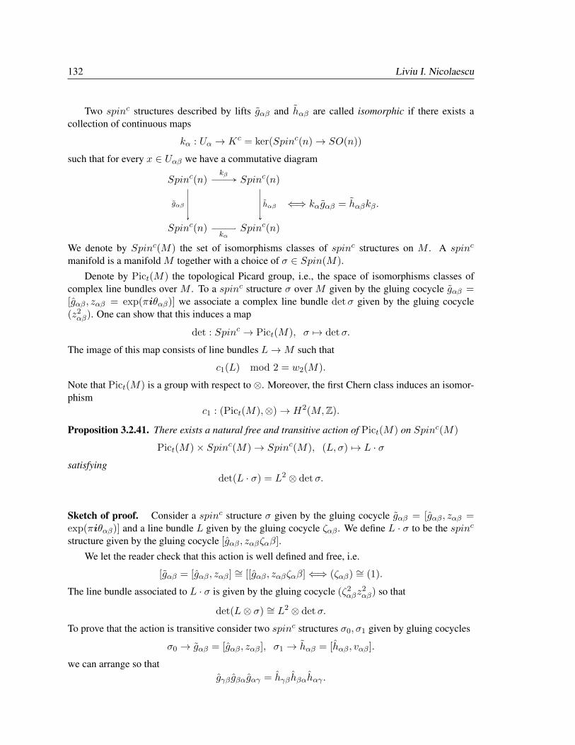
132 Liviu I. Nicolaescu
Two spinc structures described by lifts gαβ and hαβ are called isomorphic if there exists acollection of continuous maps
kα : Uα → Kc = ker(Spinc(n)→ SO(n))
such that for every x ∈ Uαβ we have a commutative diagram
Spinc(n) Spinc(n)
Spinc(n) Spinc(n)u
gαβ
wkβ
uhαβ
wkα
⇐⇒ kαgαβ = hαβkβ.
We denote by Spinc(M) the set of isomorphisms classes of spinc structures on M . A spinc
manifold is a manifold M together with a choice of σ ∈ Spin(M).
Denote by Pict(M) the topological Picard group, i.e., the space of isomorphisms classes ofcomplex line bundles over M . To a spinc structure σ over M given by the gluing cocycle gαβ =[gαβ, zαβ = exp(πiθαβ)] we associate a complex line bundle detσ given by the gluing cocycle(z2αβ). One can show that this induces a map
det : Spinc → Pict(M), σ 7→ detσ.
The image of this map consists of line bundles L→M such that
c1(L) mod 2 = w2(M).
Note that Pict(M) is a group with respect to ⊗. Moreover, the first Chern class induces an isomor-phism
c1 : (Pict(M),⊗)→ H2(M,Z).
Proposition 3.2.41. There exists a natural free and transitive action of Pict(M) on Spinc(M)
Pict(M)× Spinc(M)→ Spinc(M), (L, σ) 7→ L · σ
satisfyingdet(L · σ) = L2 ⊗ detσ.
Sketch of proof. Consider a spinc structure σ given by the gluing cocycle gαβ = [gαβ, zαβ =exp(πiθαβ)] and a line bundle L given by the gluing cocycle ζαβ . We define L · σ to be the spinc
structure given by the gluing cocycle [gαβ, zαβζαβ].
We let the reader check that this action is well defined and free, i.e.
[gαβ = [gαβ, zαβ] ∼= [[gαβ, zαβζαβ]⇐⇒ (ζαβ) ∼= (1).
The line bundle associated to L · σ is given by the gluing cocycle (ζ2αβz
2αβ) so that
det(L⊗ σ) ∼= L2 ⊗ detσ.
To prove that the action is transitive consider two spinc structures σ0, σ1 given by gluing cocycles
σ0 → gαβ = [gαβ, zαβ], σ1 → hαβ = [hαβ, vαβ].
we can arrange so thatgγβ gβαgαγ = hγβhβαhαγ .
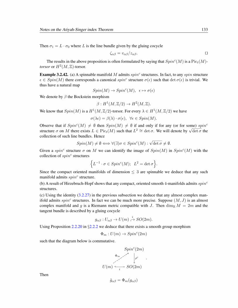
Notes on the Atiyah-Singer index Theorem 133
Then σ1 = L · σ0 where L is the line bundle given by the gluing cocycle
ζαβ = vαβ/zαβ. ut
The results in the above proposition is often formulated by saying that Spinc(M) is a Pict(M)-torsor or H2(M,Z)-torsor.
Example 3.2.42. (a) A spinnable manifoldM admits spinc structures. In fact, to any spin structureε ∈ Spin(M) there corresponds a canonical spinc structure σ(ε) such that detσ(ε) is trivial. Wethus have a natural map
Spin(M)→ Spinc(M), ε 7→ σ(ε)
We denote by β the Bockstein morphism
β : H1(M,Z/2)→ H2(M,Z).
We know that Spin(M) is a H1(M,Z/2)-torsor. For every λ ∈ H1(M,Z/2) we have
σ(λε) = β(λ) · σ(ε), ∀ε ∈ Spin(M).
Observe that if Spinc(M) 6= ∅ then Spin(M) 6= ∅ if and only if for any (or for some) spinc
structure σ on M there exists L ∈ Pict(M) such that L2 ∼= detσ. We will denote by√
detσ thecollection of such line bundles. Hence
Spin(M) 6= ∅ ⇐⇒ ∀(∃)σ ∈ Spinc(M) :√
detσ 6= ∅.Given a spinc structure σ on M we can identify the image of Spin(M) in Spinc(M) with thecollection of spinc structures
L−1 · σ ∈ Spinc(M); L2 = detσ.
Since the compact oriented manifolds of dimension ≤ 3 are spinnable we deduce that any suchmanifold admits spinc structure.
(b) A result of Hirzebruch-Hopf shows that any compact, oriented smooth 4-manifolds admits spinc
structures.
(c) Using the identity (3.2.27) in the previous subsection we deduce that any almost complex man-ifold admits spinc structures. In fact we can be much more precise. Suppose (M,J) is an almostcomplex manifold and g is a Riemann metric compatible with J . Then dimRM = 2m and thetangent bundle is described by a gluing cocycle
gαβ : Uαβ → U(m)i→ SO(2m).
Using Proposition 2.2.20 in §2.2.2 we deduce that there exists a smooth group morphism
Φm : U(m)→ Spinc(2m)
such that the diagram below is commutative.
Spinc(2m)
U(m) SO(2m)uρc
\\\\]Φm
y wi
.
Thengαβ = Φm(gαβ)

134 Liviu I. Nicolaescu
defines a spinc structure onM called the spinc structure associated to an almost complex structure.We will denote it by σC. Observe that we have a commutative diagram
Spinc(2m)
U(m) S1uu
Φm
wdet
,
where we recall that the vertical arrow is given by [g, z] 7→ z2. This shows that the line bundleassociated to σC is given by the gluing cocycle det gαβ . It is therefore isomorphic to
detC(TM, J) ∼= K−1M .
HencedetσC ∼= K−1
M .
We deduce that an almost complex manifold is spinnable iff√KM 6= ∅ and we can bijectively
identify the spin structures with the square roots of the canonical line bundle. ut
Suppose (M, g) is a compact oriented Riemann manifold of even dimension dimRM = 2m.Assume the tangent bundle is defined by a gluing cocycle
g•• : U•• → SO(2m)
Fix a spinc-structure σ ∈ Spinc(M) described by a gluing cocycle
g•• = [g••, z••] : U•• → Spinc(2m).
We denote by Pσ the principal Spinc(2m) bundle determined by this cocycle so that
TM ∼= Pσ ×ρc R2m.
The group Spinc(2m) can be naturally viewed as a subgroup in Cl2m⊗C ⊂ EndC(S2m) and assuch we have representations
ϕc± : Spinc(2m)→ AutC(S±2m), ϕc ∼= ϕc+ ⊕ ϕc−.
DefineSσ := Pσ ×ϕc S2m.
As in the previous section we see that Sσ has a natural structure of Cl(T ∗M)-module. Moreover, ifwe fix a Spinc(2m)-invariant metric on S2m then the induced Clifford multiplication
c : T ∗M → EndC(Sσ)
is odd and skew-symmetric with respect to the induced metric on Sσ.
Suppose that the Levi-Civita connection on TM is described by a collection
Aα ∈ Ω1(Uα)⊗ so(2m), Aβ = gβαAαg−1βα − dgβα · g
−1βα .
We denote by ρ∗ : spin(2m) → so(2m) the differential of ρ : Spin(2m) → SO(2m) describedexplicitly in (2.2.9) and set
Aα := ρ−1∗ (Aα) ∈ Ω1(Uα)⊗ spin(2m).
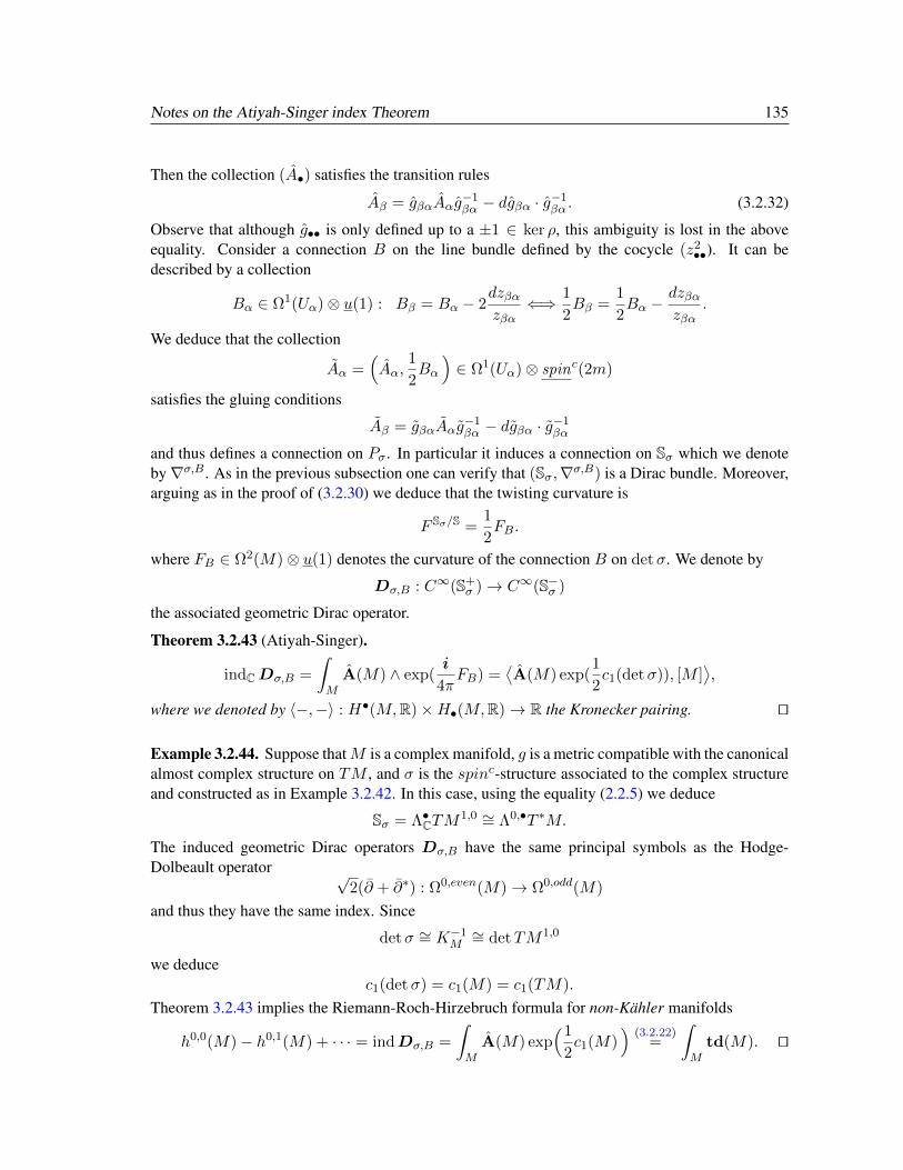
Notes on the Atiyah-Singer index Theorem 135
Then the collection (A•) satisfies the transition rules
Aβ = gβαAαg−1βα − dgβα · g
−1βα . (3.2.32)
Observe that although g•• is only defined up to a ±1 ∈ ker ρ, this ambiguity is lost in the aboveequality. Consider a connection B on the line bundle defined by the cocycle (z2
••). It can bedescribed by a collection
Bα ∈ Ω1(Uα)⊗ u(1) : Bβ = Bα − 2dzβαzβα
⇐⇒ 1
2Bβ =
1
2Bα −
dzβαzβα
.
We deduce that the collection
Aα =(Aα,
1
2Bα
)∈ Ω1(Uα)⊗ spinc(2m)
satisfies the gluing conditions
Aβ = gβαAαg−1βα − dgβα · g
−1βα
and thus defines a connection on Pσ. In particular it induces a connection on Sσ which we denoteby∇σ,B . As in the previous subsection one can verify that (Sσ,∇σ,B) is a Dirac bundle. Moreover,arguing as in the proof of (3.2.30) we deduce that the twisting curvature is
F Sσ/S =1
2FB.
where FB ∈ Ω2(M)⊗ u(1) denotes the curvature of the connection B on detσ. We denote by
Dσ,B : C∞(S+σ )→ C∞(S−σ )
the associated geometric Dirac operator.
Theorem 3.2.43 (Atiyah-Singer).
indCDσ,B =
∫M
A(M) ∧ exp(i
4πFB) =
⟨A(M) exp(
1
2c1(detσ)), [M ]
⟩,
where we denoted by 〈−,−〉 : H•(M,R)×H•(M,R)→ R the Kronecker pairing. ut
Example 3.2.44. Suppose thatM is a complex manifold, g is a metric compatible with the canonicalalmost complex structure on TM , and σ is the spinc-structure associated to the complex structureand constructed as in Example 3.2.42. In this case, using the equality (2.2.5) we deduce
Sσ = Λ•CTM1,0 ∼= Λ0,•T ∗M.
The induced geometric Dirac operators Dσ,B have the same principal symbols as the Hodge-Dolbeault operator √
2(∂ + ∂∗) : Ω0,even(M)→ Ω0,odd(M)
and thus they have the same index. Since
detσ ∼= K−1M∼= detTM1,0
we deducec1(detσ) = c1(M) = c1(TM).
Theorem 3.2.43 implies the Riemann-Roch-Hirzebruch formula for non-Kahler manifolds
h0,0(M)− h0,1(M) + · · · = indDσ,B =
∫M
A(M) exp(1
2c1(M)
)(3.2.22)
=
∫M
td(M). ut
136 Liviu I. Nicolaescu
3.3. Exercises for Chapter 3
Exercise 3.3.1. Prove (3.1.1). ut
Exercise 3.3.2. Prove (3.2.11). ut
Exercise 3.3.3. Prove Proposition 3.2.6. ut
Exercise 3.3.4. Prove the identity (3.2.14). ut
Exercise 3.3.5. Prove the identity (3.2.15). ut
Exercise 3.3.6. Prove Proposition 3.2.12. ut
Exercise 3.3.7. Prove Lemma 3.2.20.
ut
Exercise 3.3.8. Suppose that Σ is a compact, oriented Riemann surface, L → Σ is a complex linebundle equipped with a hermitian metric h and a connection ∇ compatible with h. Denote by F∇the curvature of∇ so that F∇ ∈ Ω2(Σ)⊗ C. Prove that
i
2π
∫ΣF∇ ∈ Z.
This integer is independent of the connection, it is called the degree of L, and it is denoted by degL.ut
Exercise 3.3.9. Suppose that Σ is a compact Riemann surface (compact oriented surface equippedwith a complex structure.) Assume that p1, . . . , pk is a collection of distinct points on Σ and
D =k∑j=1
njδpj , nj ∈ Z,
is a divisor supported at these points. Pick disjoint coordinates neighborhoods Uj of pj and aholomorphic coordinate zj on Uj such that zj(pj) = 0. Define
fj : U∗j := Uj \ pj → C, fj(zj) = znjj .
SetU0 = Σ \ p1, . . . , pk, A = 0, 1, . . . , k,
and denote by f0 the function f0 : U0 → C, f0 ≡ 1. For any α, β ∈ A such that Uα ∩ Uβ 6= ∅define the holomorphic function
gβα : Uα ∩ Uβ → C∗ = GL1(C), gβα =fβfα.
The collection (gβα) is a gluing cocycle for a holomorphic bundle L(D)→ Σ. Prove that
degL(D) = degD :=
k∑j=1
nj ,

Notes on the Atiyah-Singer index Theorem 137
where degL(D) is the integer defined in Exercise 3.3.8. ut
Exercise 3.3.10. Suppose that Σ is a compact Riemann surface, L → Σ is a holomorphic linebundle equipped with a Hermitian metric h. Fix a nontrivial holomorphic section u : Σ→ L.
(a) Suppose that p ∈ Σ is a zero of u, u(p) = 0. We can find a coordinate neighborhood U of pequipped with a coordinate z such that
(1) z(p) = 0
(2) There exists a holomorphic isomorphism Ψ : LU → CU , where LU denotes the restrictionof L to U and CU denotes the trivial line bundle C× U → U . We can then identify Ψ uwith a holomorphic function f : U → C.
Show that the quantity1
2πilimε0
∫|z|=ε
df
f
is an integer independent of all the choice of local coordinate z satisfying (i) and the local holomor-phic trivialization Ψ. We denote by deg(u, p) this integer.
(b) Show thatdegL =
∑u(p)=0
deg(u, p). (3.3.1)
(c) Show that the conclusion of Exercise 3.3.9 follows from (3.3.1).
(d) Show that if a holomorphic line bundle L→ Σ satisfies degL ≤ 0, then it admits no nontrivialholomorphic sections. ut
Exercise 3.3.11. Suppose that (M, g) is an oriented Riemann manifold of dimension n = 2m andE → M is a Clifford bundle. Prove E admits a connection compatible with both the metric on Eand the Clifford multiplication.
Hint: Assume first that M is spinnable. Reduce the general case to this case using partitions ofunity. ut
Exercise 3.3.12. (a) Show that we have an isomorphism of Z/2-graded algebras
Cl4 ∼= EndH(H2).
(b) Equip H2 with the complex structure defined by Ri so as a complex vector space we haveH2 ∼= C4. Prove that
Cl4⊗C ∼= EndC(H2).
(c) Show that Spin(4) ⊂ Cl4 can be identified via the isomorphism Cl4 ∼= EndH(H2) with thediagonal subgroup
Diag(q1, q2); |q1| = |q2| = 1.
ut
Exercise 3.3.13. Prove Proposition 3.2.40 ut


Chapter 4
The heat kernel proof ofthe index theorem
4.1. A rough outline of the strategy
To understand the main idea behind the heat equation approach to the index theorem we describe itin a simple finite dimensional situation.
4.1.1. The heat equation approach: a baby model. Suppose that U± are two finite dimensionalcomplex Hermitian vector spaces and
D : U+ → U−
is a complex linear operator. Then the equalities
R(D) = (kerD∗)⊥, R(D∗) = (kerD)⊥
imply that D induces an isomorphism D : R(D∗)→ R(D) and thus
indD = dim kerD − dim kerD∗ = dimU+ − dimU−.
Let us present a rather complicate alternate proof of this equality which has the advantage that itextends to infinite dimensions.
Set U := U+ ⊕U− and denote by D the operator
D =
[0 D∗
D 0
]: U → U . (4.1.1)
This is a symmetric a operator and observe that
D2 =
[D∗D 0
0 DD∗
].
The operator D2 is nonnegative so that
spec(D2) ⊂ [0,∞).
139
140 Liviu I. Nicolaescu
Moreover for any µ ≥ 0 we have
ker(µ−D2) = ker(√µ−D)⊕ ker(
õ+ D).
On the other hand, D2 commutes with the grading
γ =
[1U+ 0
0 −1U−
]: U → U
so that for any eigenvalue λ of D2 the corresponding eigenspace Eλ = ker(λ − D2) admits anorthogonal direct sum decompostion
Eλ = E+λ ⊕ E
−λ , E±λ := Eλ ∩U±.
Here is the key observation behind the heat equation approach to the index formula.
Lemma 4.1.1. For any nonzero eigenvalue λ of D we have
dimE+λ = dimE−λ .
More precisely, the restriction of D to E+λ defines a linear isomorphism
D : E+λ → E−λ .
Proof. Observe that D commutes with D2 so that Eλ is D-invariant,
DEλ ⊂ Eλ.Since λ 6= 0 we deduce that the restriction of D to Eλ is injective so that the map D : Eλ → Eλis a linear isomorphism. From the description (4.1.1) of D we deduce that the above isomorphisminduces two isomorphisms
D : E+λ → E−λ , D∗ : E−λ → E+
λ .
ut
From the equalitiesU± =
⊕λ∈spec(D2)
E±λ
we deduce that for any t ≥ 0 we have
str e−tD2
=∑
λ∈spec(D2)
e−tλ(dimE+
λ − dimE−λ ).
For t > 0 Lemma 4.1.1 implies that
str e−tD2
= dimE+0 − dimE−0 = dim kerD∗D − dim kerDD∗
= dim kerD − dim kerD∗ = indD.
ThusindD = lim
t0str e−tD
2= str1U = dimU+ − dimU−.
In the infinite dimensional case, when D is a geometric Dirac operator on a Riemann manifold(M, g), we can express str e−tD
2, t > 0, as an integral over M ,
str e−tD2
=
∫MρtdVg, ρt ∈ C∞(M),

Notes on the Atiyah-Singer index Theorem 141
and moreover, we can describe quite explicitly the limit ρ0 = limt0 ρt thus arriving at an equalityof the type
indD = limt0
str e−tD2
=
∫Mρ0dVg.
4.1.2. What really goes into the proof. Suppose that D : C∞(E+) → C∞(E−) is a Dirac typeoperator acting between two Hermitian vector bundles on the compact, oriented Riemann manifold(M, g), dimM = n. As usual we denote by D the operator
D =
[0 D∗
D 0
]: C∞(E)→ C∞(E), E = E+ ⊕ E−.
We already observe the first obstacle, namely the spectral properties of D . Fortunately, we have thefollowing result.
Fact 1. The spectrum of D2 is a discrete subset of [0,∞), and there exists a Hilbert orthonormalbasis of L2(E) consisting of eigen-sections of D2. Moreover, for any λ ∈ spec(D) the eigenspaceEλ = ker(λ−D) is finite dimensional, it is contained in C∞(E) and decomposes as an orthogonaldirect sum
Hλ = H+λ ⊕H−λ , H±λ := Hλ ∩ C∞(E±). ut
We havespec D2 =
λ ∈ [0,∞; ±
√λ ∈ spec D
.
and one can show easily that for any λ ∈ spec(D2) we have
H±λ = ker(λ−∆±),
while for λ ∈ spec(D2), λ 6= 0 the operator D induces an isomorphism
D : H+λ →H−λ .
Denote by Pλ the orthogonal projection onto Hλ. For L > 0 set
UL =⊕λ≤L
Hλ
and denote by PL the orthogonal projection onto UL,
PL =∑λ≤L
Pλ.
Denote by π0, π1 : M ×M →M , the natural projections given by
π0(p0,p1) = p0, π1(p0,p1) = p1.
For complex vector bundles E0, E1 →M we define a vector bundle E0E1 →M ×M by setting
E0 E1 := π∗0E0 ⊗ π∗1E1.
For any section Ψ ∈ C∞(E) we denote by Ψ∗ ∈ C∞(E∗) the section corresponding to Ψ viathe conjugate linear isomorphism E → E∗. Two sections Ψ0,Ψ1 ∈ C∞(E) define a sectionΨ0 Ψ∗1 ∈ C∞(E E∗) given by
Ψ0 Ψ∗1(p0,p1) = Ψ0(p0)⊗Ψ∗1(p1) ∈(E E∗
)(p0,p1)
= Ep0⊗ E∗p1
∼= Hom(Ep1, Ep0
).
For each λ ∈ spec(D2) fix an orthonormal basis
142 Liviu I. Nicolaescu
4.2. The heat kernel
4.2.1. Spectral theory of symmetric elliptic operators. To fix things, suppose that (M, g) is acompact oriented Riemann manifold of dimension n, E →M is a complex vector bundle equippedwith a Hermitian metric h a connection ∇ compatible with the metric h. In the sequel, all theSobolev norms will be defined in terms of these data.
Finally, let as assume that D : C∞(E) → C∞(E) is a symmetric elliptic operator of order `.For every r ∈ R the operator Dr := D − r is also a symmetric elliptic operator of order `. It is alsosymmetric if r ∈ R. Hence
ker(
Dr : L`,2(E)→ L2(E))⊂ C∞(E),
and for this reason we will use the simpler notation
ker Dr := ker(
Dr : L`,2(E)→ L2(E)).
Theorem 2.1.29 implies that dim ker Dr <∞, ∀r ∈ C.
Definition 4.2.1. An eigenvalue of D is a complex number λ such that
ker(
D − λ)6= 0.
The spectrum of D , denoted by spec(D), is the collection of eigenvalues of D . ut
The above discussion implies immediately the following result.
Proposition 4.2.2. The spectrum of D is contained in the real axis. Moreover, for any λ ∈ spec(D)we have
ker(D − λ) ⊂ C∞(E), dim ker(D − λ) <∞. ut
Observe thatλ 6= λ′ ⇒ ker(D − λ) ⊥ ker(D − λ′),
andspec(D) = r + spec(Dr). (4.2.1)
We have the following fundamental result.
Theorem 4.2.3 (Spectral Theorem). (a) The spectrum of D is a discrete nonempty subset of R.
(b) For any λ ∈ spec(D) we denote by Pλ the orthogonal projection onto ker(D − λ). Then forany u ∈ L2(E) we have
u =∑
λ∈spec(D)
Pλu, ‖u‖2L2 =∑
λ∈spec(D)
‖Pλu‖2L2 .
(c)u ∈ L`,2(E)⇐⇒
∑λ∈spec(D)
λ2‖Pλu‖2L2 ,
and if u ∈ L`,2(E), thenDu =
∑λ∈spec(D)
λPλu.
Notes on the Atiyah-Singer index Theorem 143
Proof. We will cary the proof in several stages.
Lemma 4.2.4. R \ spec(D) 6= ∅, i.e., there exists r ∈ R such that ker Dr = 0.
Proof. We argue by contradiction. Suppose that ker Dr 6= 0 for any r ∈ R. Since Dr is ellipticwe deduce that ker Dr ⊂ C∞(E). Hence we can find a sequence (uν)ν>0 of smooth sections of Esuch that
‖un‖L2 = 1, Duν =1
νuν , ∀ν > 0.
Since uν ⊥ ker D , ∀ν > 0, we deduce that there exists a constant C > 0 such that
‖uν‖L`,2 ≤ C‖Duν‖L2 =C
ν.
Hence uν → 0 in L`,2(E) as ν →∞. This contradicts the requirement
‖uν‖L2 = 1, ∀ν > 0.
ut
Fix r ∈ R such that ker(Dr) = 0. In view of (4.2.1) we lose no generality if we assume r = 0,i.e., D = Dr. We deduce from Theorem 2.1.29 that the induced continuous operator
D : L`,2(E)→ L2(E)
is invertible with bounded inverse
D−1L2(E)→ L`,2(E).
Denote by A the composition of D−1 with the canonical inclusion i : L`,2(E) → L2(E),
A : L2(E)D−1
−→ L1,2Ei→ L2(E).
The bounded operator A is the composition of a bounded operator with a compact operator, andthus it is compact.
Lemma 4.2.5. The operator A is selfadjoint, i.e., for any u, v ∈ L2(E) we have
(Au, v)L2 = (u,Av)L2 .
Proof. Let u, v ∈ L2(E). We can find u, v ∈ L`,2(E) such that
D u = u, D v = v.
Then Au = u , Av = v, and we deduce
(Au, v)L2 = (u,D v)L2 = (D u, v)L2 = (u,Av)L2 .
ut
Thus A is a compact, selfadjoint operator
A : L2(E)→ L2(E), kerA = 0.
Denote by spece(A) the collection of eigenvalues of A, spece(A) ⊂ R\0. For every µ ∈ spece(A)we denote by Qµ the orthogonal projection onto ker(A− µ).
144 Liviu I. Nicolaescu
Invoking the spectral theorem for compact selfadjoint operators [6, Thm. 6.11] deduce thatspece(A) is a bounded countable subset of the real axis which has a single accumulation point, 0.Moreover, for any u ∈ L2(E) we have
u =∑
µ∈spece(A)
Qµu, ‖u‖2L2 =∑
µ∈spece(A)
‖Qµu‖2L2 , (4.2.2a)
Au =∑
µ∈spece(A)
µQµu. (4.2.2b)
For each µ ∈ spece(Ar) and Ψ ∈ ker(A− µ) we have
AΨ = µΨ
so that Ψ ∈ R(A) ⊂ L`,2(E). We deduce
Ψ = DAΨ = µDΨ = µDΨ⇐⇒ DΨ = λ(µ)Ψ, λ(µ) =1
µ.
Conversely, if λ ∈ spec(D), Ψ ∈ ker(D − λ), then
DΨ = λ−Ψ, AΨ =1
λ︸︷︷︸=:µ(λ)
Ψ.
This proves that
µ ∈ spece(A)⇐⇒ λ(µ) ∈ spec(D), ker(A− µ) = ker(
D − λ(µ)).
This implies (a) and (b) of the Spectral Theorem.
To prove (c) observe first that, by construction, L`,2(E) = R(A). Thus we can find
v =∑
µ∈spece(A)
vµ ∈ L2(E), vµ ∈ ker(A− µ)
such thatu = Av =
∑µ
µvµ.
Note thatuλ := Pλu = µvµ, µ = µ(λ).
Now observe that ∑µ
‖vµ‖2L2 <∞⇒∑
λ∈spec(D)
1
µ(λ)2‖uλ‖2L2 <∞
so that ∑λ∈spec(D)
λ2‖uλ‖2L2 <∞. (4.2.3)
Conversely, if (4.2.3) holds, than
u = A
∑µ∈spece(A)
1
µ(λ)uλ
︸ ︷︷ ︸
∈L2(E)
∈ R(A) = L`,2(E).
Notes on the Atiyah-Singer index Theorem 145
Finally, ifu =
∑λ∈spec(D)
uλ ∈ L`,2(E), uλ = Pλu,
then ∑µ∈spece(A)
Qµu = u = ADu(4.2.2b)
=∑
µ∈spece(A)
µQµDu,
and we deduce Qµu = µQµDu, i.e.,
QµDu =1
µQµu and PλDu = λuλ.
HenceDu =
∑λ∈spec(D)
PλDu =∑
λ∈spec(D)
λuλ.
ut
Corollary 4.2.6. Let u ∈ L2(E),
u =∑
λ∈spec(D)
uλ, uλ = Pλu.
Thenu ∈ C∞(E)⇐⇒
∑λ∈spec(D)
λ2k‖uλ‖2L2 <∞, ∀k ∈ Zk>0.
Proof. We have
u ∈ C∞(E)⇐⇒ Dku ∈ L2(E), ∀k ∈ Z>0 ⇐⇒∑
λ∈spec(D)
λ2k‖uλ‖2L2 <∞, ∀k ∈ Z>0.
ut
Suppose now that the bundle E is Z/2-graded, E = E+ ⊕ E−, and D is a supper symmetricDirac operator, i.e., it has the form
D =
[0 D∗
D 0
]where D : C∞(E+)→ C∞(E−) is a first order elliptic operator. Observe that
D2 =
[D∗D 0
0 DD∗
].
Set∆+ = D∗D, ∆− = DD∗.
For any λ ∈ R and any µ ≥ 0 we set
Vλ = ker(λ−D),
V ±µ := ker(µ−∆±) ⊂ C∞(E±), N±µ = dim ker(µ−∆±),
V µ = V +µ ⊕H−µ ⊂ C∞(E).
Observe that V 0 = ker D2 = ker D , and V µ = ker(µ−D2). In general for any µ > 0 we have anatural inclusion
V√µ ⊕ V−√µ ⊂ V µ.
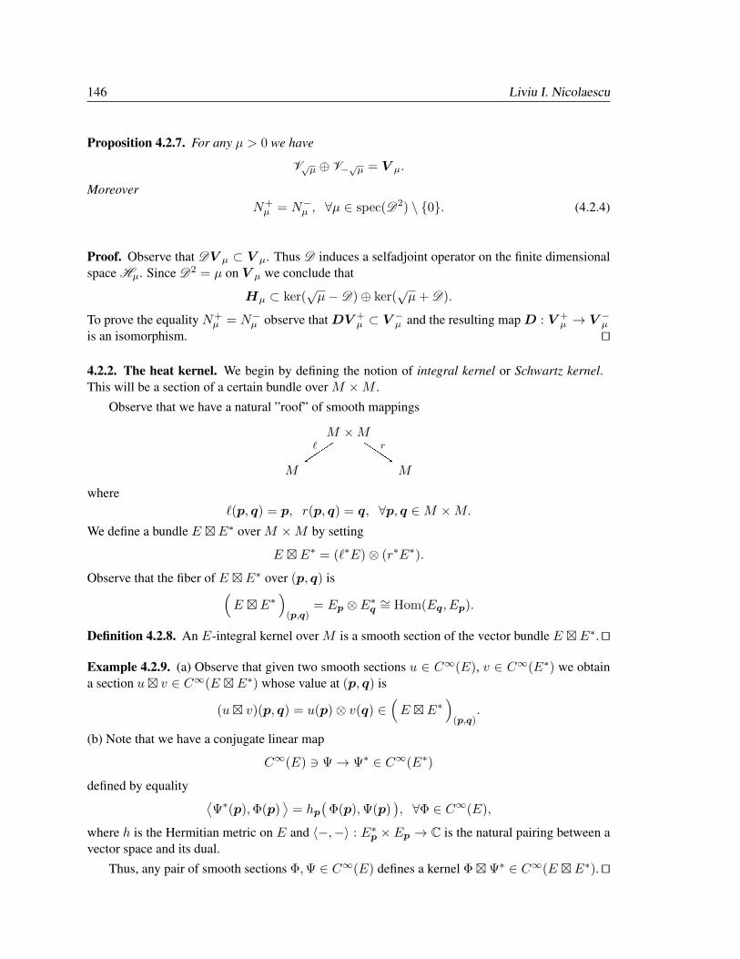
146 Liviu I. Nicolaescu
Proposition 4.2.7. For any µ > 0 we have
V√µ ⊕ V−√µ = V µ.
MoreoverN+µ = N−µ , ∀µ ∈ spec(D2) \ 0. (4.2.4)
Proof. Observe that DV µ ⊂ V µ. Thus D induces a selfadjoint operator on the finite dimensionalspace Hµ. Since D2 = µ on V µ we conclude that
Hµ ⊂ ker(√µ−D)⊕ ker(
õ+ D).
To prove the equality N+µ = N−µ observe that DV +
µ ⊂ V −µ and the resulting map D : V +µ → V −µ
is an isomorphism. ut
4.2.2. The heat kernel. We begin by defining the notion of integral kernel or Schwartz kernel.This will be a section of a certain bundle over M ×M .
Observe that we have a natural ”roof” of smooth mappings
M ×M
M M
[[[
`''')r
where`(p, q) = p, r(p, q) = q, ∀p, q ∈M ×M.
We define a bundle E E∗ over M ×M by setting
E E∗ = (`∗E)⊗ (r∗E∗).
Observe that the fiber of E E∗ over (p, q) is(E E∗
)(p,q)
= Ep ⊗ E∗q ∼= Hom(Eq, Ep).
Definition 4.2.8. An E-integral kernel over M is a smooth section of the vector bundle E E∗.ut
Example 4.2.9. (a) Observe that given two smooth sections u ∈ C∞(E), v ∈ C∞(E∗) we obtaina section u v ∈ C∞(E E∗) whose value at (p, q) is
(u v)(p, q) = u(p)⊗ v(q) ∈(E E∗
)(p,q)
.
(b) Note that we have a conjugate linear map
C∞(E) 3 Ψ→ Ψ∗ ∈ C∞(E∗)
defined by equality ⟨Ψ∗(p),Φ(p)
⟩= hp
(Φ(p),Ψ(p)
), ∀Φ ∈ C∞(E),
where h is the Hermitian metric on E and 〈−,−〉 : E∗p × Ep → C is the natural pairing between avector space and its dual.
Thus, any pair of smooth sections Φ,Ψ ∈ C∞(E) defines a kernel ΦΨ∗ ∈ C∞(E E∗).ut
Notes on the Atiyah-Singer index Theorem 147
Observe that if K ∈ C∞(E E∗) is an integral kernel and u ∈ C∞(E), then for any (p, q) ∈M ×M we obtain a linear operator K(p, q) : Eq → Ep, and a vector
K(p, q)u(q) ∈ Ep.
In particular, we obtain a smooth map
M 3 q 7→ K(p, q)u(q) ∈ Ep
which we can integrate to obtain another vector in Ep,∫MK(p, q)u(q)dVg(q) ∈ Ep.
The correspondence
M 3 p 7→∫MK(p, q)u(q)dVg(q) ∈ Ep
is then a smooth section of E. We have thus produced a linear map
IK : C∞(E)→ C∞(E), IKu(p) =
∫MK(p, q)u(q)dVg(q).
The operator IK is called the smoothing operator determined by the integral kernel K.
Observe that IK extends as a linear operator
IK : L2(E)→ C∞(E).
because the integral ∫MK(p, q)u(q)dVg(q)
can be differentiated in the p-variable as many times as we wish for any u ∈ L2(E).
Example 4.2.10. Let λ ∈ spec(D). Set
mλ := dim Vλ = dim ker(D − λ)
and denote by Pλ the orthogonal projection onto Vλ. Fix an orthonormal basis Ψ1, . . . ,Ψmλ ofker(D − λ) and define
Eλ :=
mλ∑j=1
Ψj Ψ∗j ∈ C∞(E E∗). (4.2.5)
Observe that for any u ∈ C∞(E) we have
IEλu =∑j
Ψj(p)
∫Mh(u(q),Ψj(q)
)dVg(q),
∑j
(u,Ψj
)L2Ψj = Pλu. ut
To proceed further we define a family of norms on C∞(E). More precisely, for u ∈ C∞(E)and k > 0 we set
‖u‖2k = ‖u‖2L2 + ‖Dku‖2L2 .
For uniformity we set‖u‖0 := ‖u‖L2 .
The elliptic estimates for D imply that for any k ≥ 0, there exists Ck ≥ 1 such that1
Ck‖u‖Lk,2 ≤ ‖u‖k ≤ Ck‖u‖Lk,2 .
148 Liviu I. Nicolaescu
The above equality shows that the closure of C∞(E) in the norm ‖ − ‖k is the Sobolev spaceLk,2(E).
From the Sobolev inequalities we deduce that if m > k + n2 , then there exists C = C(m, k)
such that ∥∥u∥∥Ck≤ C
∥∥u∥∥m, ∀u ∈ C∞(E). (4.2.6)
For any compact interval I ⊂ [0,∞] we set
EI :=∑|λ|∈I
Eλ ∈ C∞(E E∗)
The smoothing operator associated to this integral kernel is the orthogonal projection PI onto thespace
HI :=⊕|λ|∈I
Vλ =∑λ∈I
V λ2 .
When I = c we setHc = Hc = V−c ⊕ Vc = V c2 .
Observe thatPI =
⊕|λ|∈I
Pλ, d(I) := dim HI =∑|λ|∈I
mλ.
Moreover, ifΨj , j = 1, . . . , d(I)
is an orthonormal basis of HI , then
EI =
d(I)∑j=1
Ψj Ψ∗j . (4.2.7)
Proposition 4.2.11. (a) Set r := rank (E). There exists a constant C0 > 0 such that
d(I) ≤ C20r volg(M)(1 + b2`0), `0 = bn/2c+ 1, ∀I = [a, b] ⊂ [0,∞). (4.2.8)
(b) For any k ≥ 0 there exists a constant Zk > 0 such that for any compact interval I = [a, b] ⊂[0,∞) we have
‖EI‖Ck ≤ Zk(1 + bpk
), pk = 2
(bn/2c+ 1 + k
). (4.2.9)
Proof. We adopt the strategy in the proof of [14, Thm. 17.5.3]. For u ∈ L2(E) we set uI := PIu.For any positive integer ` and u ∈ C∞ we have
‖uI‖2` = ‖ uI‖2 + ‖DmuI‖2 ≤ (1 + b2`)‖u‖2. (4.2.10)
For any any nonnegative integer k we set
`k :=⌊n
2
⌋+ k + 1,
so that L`k,2(E) → Ck(E). In particular, we deduce that there exists a constant Z0 > 0 such that
‖uI‖C0 ≤ Z0
(1 + b2`0
) 12 ‖u‖L2 , ∀u ∈ L2(E). (4.2.11)
Notes on the Atiyah-Singer index Theorem 149
Fix p0 ∈M , and e ∈ Ep0a unit length vector. We set
Vp0,ε(q) =
d(I)∑j=1
h(e,Ψj(p0)
)Ψj(q) ∈ C∞(E).
From the equalityuI(p0) =
∑j
(u,Ψj)L2Ψj(p0), u ∈ L2∞(E)
we deduceh(uI(p0), e ) =
(u, Vp0,e
)L2 .
Hence for any u ∈ L2(E) we have(u, Vp0,e
)L2 = h
(uI(p0), e ) ≤ ‖uI‖C0 ≤ Z0
(1 + b`0
) 12 ‖u‖L2 .
This implies that
‖Vp0,e‖ ≤ Z0
(1 + b2`0
) 12 .
Observe that since sections (Ψj) form an orthonormal basis of HI we have
‖Vp0,e‖2 =
d(I)∑j=1
∣∣h( e,Ψj(p0)) ∣∣2 ∫
M|Ψj(q)|2dVg(q) =
d(I)∑j=1
∣∣h( e,Ψj(p0)) ∣∣2.
Let e1, . . . , er be an orthonormal frame of Ep0, r = rank (E). We deduce
r∑k=1
‖Vp0,ek‖2 =
r∑k=1
d(I)∑j=1
∣∣h( ek,Ψj(p0)) ∣∣2
=
d(I)∑j=1
r∑k=1
∣∣h( ek,Ψj(p0))∣∣2 =
d(I)∑j=1
∣∣Ψj(p0)∣∣2
Henced(I)∑j=1
∣∣Ψj(p0)∣∣2 ≤ Z2
0r(
1 + b2`0).
Integrating the above inequality we deduce (4.2.8).
Next observe that, for any Ψ ∈HI we have
‖Ψ‖`k ≤√
1 + b2`k‖Ψ‖.
Hence, there exists C = Ck > 0, independent of I , such that
‖Ψ‖Ck ≤ Ck√
1 + b2`k‖Ψ‖, ∀Ψ ∈HI .
From the equality (4.2.7) we deduce that
‖EI‖Ck ≤d(I)∑j=1
‖Ψj‖2Ck ≤ Ckd(I)(1 + b2`k) ≤ Z20rCk volg(M)
(1 + b2`0
)(1 + b2`k)
≤ Zk(
1 + b2(`0+`k)).
150 Liviu I. Nicolaescu
We have reached the desired conclusion since
pk = 2(`0 + `k).
ut
For any continuous and bounded function f : R→ R we have a bounded linear operator
f(D) : L2(E)→ L2(E), f(D)u =∑
λ∈spec(D)
f(λ)Pλu.
The series ∑λ∈spec(D)
f(λ)Pλu
converges in L2(E) because∑λ
|f(λ)|2‖Pλu‖2 ≤(
supt∈R|f(t)|2
)‖u‖2.
Proposition 4.2.12. Suppose that f : R→ R is a continuous function with fast decay at∞, i.e.,
lim|λ|→∞
|λ|kf(λ) = 0, ∀k > 0.
Then f(D) is the smoothing operator determined by the integral kernel
Kf =∑
λ∈spec(D)
f(λ)Eλ.
Proof. For any ν ∈ Z≥0 we set
Kf,ν =∑
|λ|∈[ν,ν+1]
f(λ)Eλ,
where for simplicity we set Eλ = 0 if λ 6∈ spec(D). This is an integral kernel. Let us show that∑ν≥0
Kf,ν
converges in Ck(E × E∗) for any positive integer k. Set
dν := dim H[ν,ν+1], fν := sup|t|∈[ν,ν+1]
|f(t)|
Observe that‖Kf,ν‖Ck ≤
(sup
|t|∈[ν,ν+1]|f(t)|
) ∑|λ|∈[ν,ν+1|
‖Eλ‖Ck
(4.2.9)
≤ Zkfνdν(
1 + ν)pk (4.2.8)
≤ Z ′kfν(
1 + ν)2`0+pk .
Since f is fast decaying we deduce that∞∑ν=0
fν(
1 + ν)2`0+pk <∞.
ut
Notes on the Atiyah-Singer index Theorem 151
The function ft(λ) = e−tλ2
is fast decaying for any t > 0. Thus, for t > 0 the operator
ft(D) = e−tD2
is smoothing. We denote by Kt the integral kernel of this operator.
Definition 4.2.13. The collection of integral kernels (Kt)t>0 is called the heat kernel associated tothe Dirac operator D . ut
Denote by π the natural projection R>0×M ×M →M ×M . The collection (Kt)t>0 definesa section K of the pullback
E E∗ := π∗(E E∗
).
Proposition 4.2.14. (a) The heat kernel defines a smooth section of the bundle
E E∗ → R>0 ×M ×M.
(b) For any q ∈M , fixed, we have
∂tKt(p, q) + D2pKt(p, q) = 0, (4.2.12)
where Dp indicates that the operator D acts only on the variable p.
(c) If u ∈ C∞(E) andut := e−tD
2u = IKtu,
thenlimt0‖ut − u‖C0 = 0.
Proof. For any positive integer N we set
Kt,N (p, q) =∑|λ|≤N
e−tλ2Eλ(p, q).
This is a smooth function for any N and the proof of Proposition 4.2.12 shows that for any k > 0Kt,N converges to Kt as N → ∞ in the Ck-topology, uniformly for t on the compacts of R>0.Moreover (
∂t + D2p
)Kt,N = 0,
becauseD2
pEλ = λ2Eλ.
The integral kernels D2pKt,N converge in any Ck-topology to the smooth integral kernel associated
to the fast decaying function λ 7→ λ2e−tλ2. It does so uniformly for t on compacts of R>0. This
proves that Kt is C1 and∂tKt = −D2Kt.
Iterating this procedure we deduce that Kt is smooth in all variables and
∂kt Kt = (−1)kD2kp Kt.
To prove (c), let u ∈ C∞(E). Then
u =∑
λ∈spec(D)
uλ, uλ = Pλu.
152 Liviu I. Nicolaescu
For any positive integer m we have
‖u‖2m = ‖Dmu‖2 =∑λ
|λ|2m‖uλ‖2 <∞.
Observe thatut =
∑λ∈spec(D)
e−tλ2uλ
and‖ut − u‖2m =
∑λ∈spec(D)
(e−tλ
2 − 1)2|λ|2m‖uλ‖2.
Aplying the dominated convergence theorem to the functions
ϕt : spec(D)→ R, ϕt(λ) =(e−tλ
2 − 1)2|λ|2m‖uλ‖2,
where spec(D) is equipped with the canonical discrete measure, we deduce
limt0‖ut − u‖2m = 0, ∀m.
We obtain the desired conclusion by invoking the Morrey-Sobolev embedding theorem. ut
Theorem 4.2.15. The heat kernel is the unique smooth section (Kt)t>0 of
E E∗ → R>0 ×M ×M
satisfying the following properties.
(a) The integral kernel Kt(p, q) satisfies the heat equation (4.3.4) for any q fixed.
(b) If u ∈ C∞(E) we have
limt0‖IKtu− u‖C0 = 0.
Proof. The proof is based on the following uniqueness result.
Lemma 4.2.16. Denote by E the pullback of the bundle E → M over the cylinder [0,∞) ×M .For any u0 ∈ C∞(E) the initial value problem
(∂t + D2)u(t,p) = 0, u(0,p) = u0(p), ∀p ∈M (4.2.13)
admits a unique solution u which is a continuous section of E on [0,∞) × M and smooth on(0,∞)×M .
Proof. Denote by ut the restriction of u to t ×M . It suffices to show that if u0 = 0 then ut = 0,∀t > 0. We have
d
dt‖ut‖2 = (u′t, ut)L2 + (ut, u
′t)L2 = −(D2ut, ut)L2 − (ut,D
2)L2 = −2‖Dut‖2 ≤ 0.
Hence0 ≤ ‖ut‖ ≤ ‖u0‖ = 0, ∀t > 0.
ut
Notes on the Atiyah-Singer index Theorem 153
The above Lemma and the results proven so far show that the unique solution of the inial valueproblem (4.2.13) is
ut = e−tD2u0.
Suppose now that we have a family of integral kernels (Kt)t>0 satisfying the conditions (a), (b) inthe theorem. For any u ∈ C∞(E) and t > 0 set
ut = IKtu.
For ε > 0, the sections vt = ut+ε satisfy the initial value problem
(∂t + D2)vt = 0, vt=0 = uε.
Hence vt = e−t2D2
uε, i.e.,IKt+εu0 = e−tD
2uε.
If we let ε 0 we deduce
IKtu0 = e−tD2u0 = IKtu0, ∀u0 ∈ C∞(E).
This implies Kt = Kt, ∀t > 0. ut
4.2.3. The McKean-Singer formula. Recall that
D2 = ∆+ ⊕∆−, ∆+ = D∗D, ∆− = DD∗.
For any µ ∈ V µ = ker(µ−D2) we choose an orthonormal basis
Ψ±1,µ, . . . ,Ψ±N±µ∈ C∞(E±) ⊂ C∞(E)
of V ±µ = ker(µ−∆±). The collectionΨ±j,µ; µ ∈ spec(D2), 1 ≤ j ≤ N±µ
is an orthonormal basis of L2(E). We have
e−tD2
=∑
µ∈spec(D2
e−tµ(PV +
µ+ PV −µ
)where U denotes the orthogonal projection onto a closed subspace U ⊂ L2(E).
The Schwartz kernel of PV ±µis
K±µ (p, q) =
N±µ∑j=1
Ψ±j,µ(p)Ψ±j,µ(q)∗.
From the equalityV +µ ⊕ V −µ = V−√µ ⊕ V√µ
we deduceK+µ (p, q) +K−µ (p, q) = E−√µ(p, q) + E√µ(p, q)
andKt(p, q) =
∑µ∈spec(D2)
e−tµ(K+µ (p, q) +K−µ (p, q)
)︸ ︷︷ ︸=:Kµ(p,q)
∈ Hom(Eq, Ep
).
Observe that Kµ(p,p) ∈ End(Ep) and
strKµ(p,p) = trK+µ (p,p)− trK−µ (p,p)
154 Liviu I. Nicolaescu
=
N+µ∑
j=1
|Ψ+j,µ(p)|2 −
N−µ∑j=1
|Ψ−j,µ(p)|2.
Hence
str Kt(p,p) =∑
µ∈spec(D2)
e−tµ
N+µ∑
j=1
|Ψ+j,µ(p)|2 −
N−µ∑j=1
|Ψ−j,µ(p)|2 ,
so that∫M
str Kt(p,p)dVg(p) =∑
µ∈spec(D2)
e−tµ
N+µ∑
j=1
∫M|Ψ+
j,µ(p)|2dVg(p)−N−µ∑j=1
∫M|Ψ−j,µ(p)|2dVg(p)
=
∑µ∈spec(D2)
e−tµ(N+µ −N−µ )
(4.2.4)= N+
0 −N−0 .
We have thus proved the following important result.
Theorem 4.2.17 (McKean-Singer). If D : C∞(E+)→ C∞(E−) is a Dirac type operator,
D =
[0 D∗
D 0
]and Kt is the integral kernel of e−tD
2, t > 0, then
indD = N+0 −N
−0 =
∫M
str Kt(p,p)dVg(p), ∀t > 0. ut
4.3. The proof of the Index Theorem
We will use the McKean-Singer formula to give a proof of the index theorem. We will achieve thisin two conceptually different steps. First we will produce a more approximation for the heat kernel.We then show that if D is a geometric Dirac operator then the super trace of the approximation canbe understood quite explicitly.
4.3.1. Approximating the heat kernel. The approximation of the heat kernel we are able to pro-duce takes the form of an asymptotic expansion.
Definition 4.3.1. Let f be a function defined on the positive semiaxis (0,∞) and valued in a Banachspace X . A formal series
∞∑k=0
ak(t), ak : (0,∞)→ X,
is called an asymptotic expansion for f near t = 0 and we indicate this by
f(t) ∼∞∑k=0
ak(t),
if for each positive integer N there exists `N > 0 such that, for any ` ≥ `N there exists a constantC = C(`,N) and τ(`,N) > 0 such that∥∥∥∥∥f(t)−
∑k=0
ak(t)
∥∥∥∥∥ ≤ C(`,N)tN , ∀0 ≤ t ≤ τ(`,N). ut

Notes on the Atiyah-Singer index Theorem 155
We have the following important result.
Theorem 4.3.2. Suppose that (M, g) is a compact oriented Riemann manifold, E = E+ ⊕ E− →M is a Hermitian Z/2-graded vector bundle and D : C∞(E) → C∞(E) is a supersymmetricformally selfadjoint Dirac operator. Denote by Kt the heat kernel of D and by
dist : M ×M → [0,∞)
the geodesic distance function on M determined by the Riemann metric g. For any t > 0 define
ht : M ×M → R, ht(p, q) =1
(4πt)n2
exp
(−dist(p, q)2
4t
).
Then the following hold.
(a) There exists an asymptotic expansion for Kt of the form
Kt(p, q) ∼ ht(p, q)(
Θ0(p, q) + tΘ1(p, q) + t2Θ2(p, q) + · · ·),
where Θj ∈ C∞(E E∗), ∀j = 0, 1, 2, . . . .
(b) The expansion in valid in the Banach space Cr(E E∗) for any integer r ≥ 0. It maydifferentiated formally with respect to t,p, q to obtain asymptotic expansions for the cor-responding derivatives of the heat kernel Kt.
(c) The jets of the sections Θj along the diagonal are described by universal algebraic expres-sions involving the metrics, the connection coefficients and their derivatives. MoreoverΘ0(p,p) = 1Ep .
To prove the theorem we need a simple criterion for recognizing an asymptotic expansion of thehet kernel when we see one. This is based on the concept of approximate heat kernel.
Definition 4.3.3. Let m be a positive integer. An approximate heat kernel of order m for D is atime dependent section K ′t(p, q) of E E∗, t > 0 which is C1 in t and C2 in p, q and satisfyingthe following conditions.
(a) For any u ∈ C∞(E) we have
limt0‖IK′t
u− u‖C0 = 0.
(b) (∂t + D2
p
)K ′t(p, q) = tmrt(p, q), ∀t > 0, p, q ∈M,
where rt is a Cm-section of E E∗ which depends continuously on t for t ≥ 0. ut
Proposition 4.3.4. Suppose that we have a sequence of sections Θj ∈ C∞(EE∗), j = 0, 1, 2, . . . ,such that for any positive integer m there exists Jm > 0 with the property that for any J ≥ Jm theintegral kernel
KJt (p, q) = ht(p, q)
J∑j=0
tjΘj(p, q).
is an approximate heat kernel of order m. Then the formal series
ht(p, q)∞∑j=0
tjΘj(p, q)
is an asymptotic expansion for the heat kernel in the sense of (a),(b) of Theorem 4.3.2. ut

156 Liviu I. Nicolaescu
To keep the flow of arguments uninterrupted we defer the proof of this proposition.
Proof of Theorem 4.3.2. We follow the approach in [27, Chap.7]. As we know D2 has the blockform
D2 =
[∆+ 00 ∆−
]where ∆± : C∞(E±) → C∞(E±) is a formally selfadjoint generalized Laplacian. Hence thereexists metric connections ∇± on E± and Hermitian bundle endomorphisms R± : E± → E± suchthat
∆± = (∇±)∗∇± + R±.
Set ∇ = ∇+ ⊕ ∇−, R = R+ ⊕ R− so that ∇ is a metric connection on E compatible with theZ/2-grading and R is an even, Hermitian endomorphism of E. By construction
D2 = ∇∗∇+ R.
Let ∆g : C∞(M)→ C∞(M) denote the scalar Laplacian defined by the metric g. For any smoothfunction f : M → R we denote by grad f ∈ Vect(M) the gradient of f with respect to the metricg, i.e., the metric dual of df .
The symbol of D defines a Clifford multiplication on E
c : T ∗M → End(E), c(df) = [D , f ], ∀f ∈ C∞(M).
A simple computation shows that
[D2, f ]u = −2∇grad fu+ (∆gf)u, ∀u ∈ C∞(E), f ∈ C∞(M). (4.3.1)
Using Proposition 4.3.4 we seek sections Θj ∈ C∞(E E∗), j = 0, 1, 2, . . . , such that for anym > 0 the integral kernel
KJt (p, q) = ht(p, q)
J∑j=0
tjΘj(p, q)
is an approximate heat kernel of orderm for all J sufficiently large. Note that it suffices to constructΘj for p close to q because for (p, q) outside a neighborhood of the diagonal the function ht(p, q)goes to zero faster than any power of t as t→ 0.
Let us fix the point q and normal coordinates x1, . . . , xn with q as origin. We set
r2 =n∑i=1
(xi)2
so that r(x) = dist(x, 0). Observe that r∂r is the radial vector field and
grad r2 = 2r∂r, ∆gr2 = 2n− r∂r log |g|, |g| := det(gij).
With q fixed ht(p, q) becomes a function of t and r
ht =1
(4πt)n2
e−r2
4t .
Some elementary computations show that
gradht = −ht2tr∂r, (4.3.2a)
(∂t + ∆g)ht =ht4tr∂r log |g|. (4.3.2b)
Notes on the Atiyah-Singer index Theorem 157
Using (4.3.1), (4.3.2a) and (4.3.2b) we deduce that for any t-dependent smooth section v of E (orE ⊗ Eq) we have
1
ht
(∂t + D2
)(htv) = (∂t + D2)v +
r
4t(∂r log |g|)v +
1
t∇r∂rv. (4.3.3)
If we let H denote the conjugate heat operator
H :=1
ht
(∂t + D2
)ht (4.3.4)
then we can rewrite the last equality as
H = (∂t + D2) +1
t∇r∂r +
r
4t(∂r log |g|). (4.3.5)
In particular, if v = tju, u independent of t, then
H(tjv) = tj−1(∇r∂ru+ j +
r
4∂r log |g|
)u+ tjD2u. (4.3.6)
Now writeu ∼ u0 + tu1 + t2u2 + · · · ,
where uj are independent of t and attempt to solve the equation
(∂t + D2)(htu) = 0⇐⇒ Hu = 0,
by equating to zero the coefficients of powers of t that arise from the equality (4.3.6). We obtain thefollowing system of equations for j = 0, 1, 2, . . .
∇r∂ruj +
(j +
r∂r|g|4|g|
)uj = −D2uj−1. (4.3.7)
The equations (4.3.7) are just ordinary differential equations along the geodesic emanating from q
and once can solve them recursively. To do this we introduce an integrating factor |g|14 and rewrite
the equations as
∇∂r(rj |g|
14uj
)=
0, j = 0,
−rj−1|g|14 D2uj−1, j ≥ 1.
(4.3.8)
For j = 0 this shows that uj is uniquely determined by its initial value uj(0) which we fix asu0(0) = 1Eq . For j ≥ 1 the equation determines uj in terms of of uj−1 up to the addition of a termof the form Cjr
−j |g|−14 . The requirement of smoothness at q forces Cj = 0 so we conclude that all
the uj are uniquely determined by the single initial condition u0(0) = 1Eq .
Define Θj(p, q) to be the section of E E∗ over a neighborhood U of the diagonal which isrepresented in normal coordinates near q by the sections uj constructed above. Fix another smalleropen neighborhood of the diagonal V ⊂ U and a smooth function ϕ : M ×M → [0,∞) such that
ϕ(p, q) =
1, (p, q) ∈ V ,
0, (p, q∈(M ×M) \U .
Set
KJt (p, q) := ϕ(p, q)ht(p, q)
J∑j=0
tjΘj(p, q).
158 Liviu I. Nicolaescu
Since Θ0(p,p) = 1Ep we deduce that
limt0‖IKJ
tu− u‖C0 = 0, ∀u ∈ C∞(E).
Moreover, the construction of the u′j-s shows that
(∂t + D2p)KJ
t (p, q) = tJht(p, q)eJt (p, q), t > 0,
where et ∈ C∞(EE∗) depends continuously on t down to t = 0. For J > m + n2 the function
tJht(p, q) tends to zero in the Cm-topology as t→ 0. Thus, for any J > m+ n2 the integral kernel
KJt is an approximate heat kernel of order m. Invoking Proposition 4.3.4 we deduce that the formal
series
ϕ(p, q)ht(p, q)
∞∑j=0
tjΘj(p, q),
is an asymptotic expansion of the hear kernel, i.e., satisfies the conditions (a), (b) of Theorem 4.3.2.The claim (c) of the theorem follows inductively from the differential equations (4.3.8). ut
Theorem 4.3.2 has the following immediate consequence.
Corollary 4.3.5. (a) If n = dimM is odd then indD = 0.
(b) If d ImM = n = 2m is even then
indD =1
(4π)n2
∫M
str Θn2(q, q)dVg(q). ut
Thus the name of the game is determining the index density, i.e., the function
M 3 q 7→ str Θn2(q, q) ∈ R.
This is the goal of the next two subsections.
4.3.2. The Getzler approximation process. To determine the index density we will make an ad-ditional assumption. More precisely we require that D be a geometric Dirac operator. In otherwords, we require that E is equipped with an odd, skew-hermitian multiplication
c : T ∗M → End(E)
and a herminitan connection ∇ compatible with both the Z/2-grading of E and the Clifford mul-tiplication. This means that for any u ∈ C∞(E), any α ∈ C∞(T ∗M) and any vector fieldX ∈ Vect(M) we have
∇X(c(α)u
)= c(∇gXα)u+ c(α)∇Xu,
where∇g denotes the Levi-Civita connection. The operator D has the form
D = c ∇ : C∞(E)∇−→ C∞(T ∗M ⊗ E)
c−→ C∞(E),
and satisfies the Weitzenbock formula
D2 = ∇∗∇+s(g)
4+ c(FE/S),
where s(g) is the scalar curvature of g,
FE/S := F − c(R) ∈ Ω2(Cl(M)⊗EndCl(M)(E)
),
Notes on the Atiyah-Singer index Theorem 159
c(R)(ei, ej) =1
4
∑k,`
g(R(ei, ej)ek, e`
)c(ek)c(e`) ∈∈ Ω2(End(E)),
c(FE/S) =∑i<j
F e/S(ei, ej)c(ei)c(ej),
and (e1, . . . , en) is an oriented orthonormal basis of a tangent space TpM .
Fix a point q0 ∈ M , an oriented orthonormal basis e1, . . . , en of Tq0M . This basis determines
normal coordinates (x1, . . . , xn) defined on an open geodesic ballBR(q0). Using these coordinateswe identiftBR(q0) with the open ballBR(0) ⊂ Tq0
M and Tq0M with the Euclidean space Rn. Set
E0 := Eq0.
Using the ∇-parallel transport along geodesics starting at q0 we can produce a trivialization of Eover BR(q0). The functions
BR(q0) 3 p 7→ Θj(p, q0) ∈ Hom(Eq0, Ep),
can be viewed as functions
Tq0M ⊃ BR(0) 3 x 7→ Θj(x) ∈ End(E0). (4.3.9)
As such, they have Taylor expansions
Θj(x) =∑α
xαΘj,α, Θj,α ∈ End(E0).
where for any multitindex α ∈ Zn≥0 we set
xα := (x1)α1 · · · (xn)αn , |α| = |α1|+ · · ·+ |αn|.
The fiber E0 is a Z/2-graded Cl(T ∗q0M)-module and thus it has the form
E0∼= Sn⊗W
where Sn = S+n ⊕ S−n is the space of complex spinors associated to the Clifford algebra Cl(T ∗q0
M).Denote by e1, . . . , en the dual basis of T ∗q0
M . This oriented, orthonormal basis e1, . . . , en identifiesCl(T ∗q0
M) with Cln.
For every order multi-index I = (1 ≤ i1 < · · · < k ≤ N) we set |I| := k and
e∧I := ei1 ∧ · · · ∧ eik , cI := c(ei1) · · · c(eik).
From Proposition 2.2.6 we deduce that any operator T ∈ End(E0) decomposes as a sum
T =∑I
cI ⊗ TI , TI = End(W ) ∼= EndCln(E0).
We say that T has order ≤ k, ordT ≤ k, if TI = 0, for |I| > k. If ordT ≤ k we set
[T ]k =∑
|I|=ordT
e∧I ⊗ TI ∈ ΛT ∗q0M⊗End(W ) = ΛRn⊗End(W ) =: Sn(W ).
We say that ordT = k if ordT ≤ k and [T ]k 6= 0. We set
[T ] := [T ]ordT ∈ Sn(W ),
and we will refer to [T ] as the Getzler symbol of T .
160 Liviu I. Nicolaescu
Note that if T1, T2 ∈ End(E0), ordT1 ≤ k1, ordT2 ≤ k2, then ord(T1T2) ≤ k1 + k2 and
[T1T2]k1+k2 = [T1]k1 [T2]k2 .
Note that ordT ≤ n, ∀T ∈ End(E0). From Proposition 2.2.8 we deduce that
ordT < n⇒ strT = 0.
Moreover, when ordT = n = 2m, then
strT = (−2i)m strT1,2,...,n =: str[T ]n.
We can rewrite the last facts in a compact form
strT = str[T ]n, ∀T ∈ End(E0). (4.3.10)
Define the order of a monomial xα to be −|α|,ordxα := −|α|
Denote by C[[x]] the ring of formal power series in the variable (x1, . . . , xn) with complex coeffi-cients, and by R(E0) the noncommutative ring of smooth maps BR(0)→ End(E0). If T is a mapin R(E0) is a smooth map with Taylor expansion at 0 given by
T (x) ∼∑α
xαTα ∈ C[[x]]⊗ End(E0).
then we say that ordT (x) ≤ k if
ordTα − |α| = ordTα + ordxα ≤ k, ∀α.If ordT ≤ k we set
[T (x)]k :=∑
ordTα−|α|≤k
xα[Tα] ∈ C[[x]]⊗Sn(W ).
The ring C[[x]]⊗Sn(W ) can be identified with the ring Sn(W )[[x]] of formal power series in thevariable x = (x1, . . . , xn) with coefficients in the (noncomutative) ring Sn(W ). We will use thenotation
Sn(W,x) := C[[x]]⊗Sn(W ).
Hence[T (x)]k ∈ Sn(W,x).
We say that ordT (x) = k if ordT (x) ≤ k and [T (x)]k 6= 0. We set
[T (x)] = [T (x)]ordT ,
and we will refer to [T (x)] as the Getzler symbol. Note that for any smooth map T ∈ R(E0) wehave ordT (x) ≤ n and
strT (0) =(str[T (x)]n
)x=0
= str[T0]n.
We want to extend the above concept of order and symbol to differential operators. Let R(E0)[∂] bethe ring of partial differential operators with coefficients in R(E0), acting on R(E0). A differentialoperator P ∈ R(E0)[∂] can be put in the canonical form
P =∑α
Pα∂α, Pα ∈ R(E0)
where all but finitely many Pα’s are zero, and for any multi-index α we set
∂α := ∂α11 · · · ∂
αnn , ∂i := ∂xi .
Notes on the Atiyah-Singer index Theorem 161
The product of two such operators can be put in canonical form by iteratively employing the com-mutation relations
∂i T = (∂iT ) ∂0 + T∂i, ∀T ∈ R(E0), i = 1, . . . , n.
GivenP =
∑α
Pα∂α ∈ R(E0)[∂]
we say that ordP ≤ k ifordPα + |α| ≤ k.
Denote by Sn(W,x)[∂] the ring of formal partial differential operators with coefficients in Sn(W,x).If
P =∑α
Pα∂α ∈ R(E0)[∂],
and ordP ≤ k, then we set
[P ]k =∑α
[Pα]k−|α|∂α ∈ Sn(W,x)[∂].
The operator P is said to have order k if ordP ≤ k and [P ]k 6= 0. In this case we set
[P ] = [P ]k = [P ]ordP
and we say that [P ] is the Getzler symbol of P . Note that
ord ∂α = |α| [∂α] = ∂α.
Moreover if P,Q ∈ R(E0)[∂], ordP ≤ k, ordQ ≤ `, then
ordPQ ≤ k + `, [PQ]k+` = [P ]k[Q]`. (4.3.11)
Using the above trivialization of E over BR(q0), we can regard∇ as a connection on the trivialbundle E0BR(0)
and as such it has the form
∇ = ∇0 +A, A ∈ Ω1(BR(0))⊗ End(E0),
where∇0 denotes the trivial connection. Set∇i = ∇∂i and Ai = ∂i A ∈ R(E0) so that
∇i = ∂i +Ai ∈ R(E0)[∂].
We have the following elementary but miraculous consequence of the fact that∇ is compatible withthe Clifford multiplication, [4, Lemma 4.15].
Lemma 4.3.6. We have
Ai =1
4
∑j,k<`
Rk`ijxjckc` +
∑k<`
fik`(x)ckc` + gi(x),
where R is the Riemann curvature of g
Rijk` = gq0(ei, R(ek, e`)ej),
fik` ∈ C∞(BR(0)), ord fik` ≤ −2,
andgi : BR(0)→ End(W )
is a smooth function such that gi(x) = O(|x|) as x→ 0 so that ord gi ≤ −1. ut
162 Liviu I. Nicolaescu
Using Lemma 4.3.6 we deduce that ord∇i ≤ 1 and we observe that the Getzler symbol of ∇iis
[∇i]1 = ∂i + [Ai]1 = ∂i +1
4
∑j
∑k<`
Rk`ijxjek ∧ e`. (4.3.12)
We setRij :=
∑k<`
Rk`ijek ∧ e` ∈ Λ2Rn, ∀i, j
so that we can rephrase (4.3.12) as
[∇i]1 = ∂i + [Ai]1 = ∂i +1
4
∑j
xjRijxj . (4.3.13)
Observe that
D =n∑i=1
ci∇i.
Since ord ci ≤ 1 and ∇icj = 0 at 0, we deduce from (4.3.11) that ord D ≤ 2 and
[D ]2 =∑i
ei∂i +1
4
∑i
∑j,k<`
Rk`ijxjei ∧ ek ∧ e` ∈ Sn(W,x)[∂].
In particular, we deduce that ord D2 ≤ 4. In fact, we can do a lot better.
Proposition 4.3.7. ord D2 = 2 and
[D ]2 = −∑i
[∇i]2 = −∑i
∂i +1
4
∑j
xjRij
2
+ FE/S ∈ Sn(W,x)[∂]. (4.3.14)
Proof. From the Weitzenboock formula we deduce
D2 = ∇∗∇+s(g)
4+ c(FE/S
)= ∇∗∇+
s(g)
4+∑i<j
FE/S(ei, ej)c(ei)c(ej).
SinceFE/S(ei, ej) ∈ EndCln(E0) = End(W ),
we deduce that
ord c(FE/S
)= 2, [c
(FE/S
)] =
∑i<j
FE/S(ei, ej)ei ∧ ej = FE/S.
Note that ord s(g) ≤ 0. On the other hand,
∇∗∇ = −∑i,j,k
gjk(∇j∇k − Γijk∇i),
where Γijk are the Christoffel symbols of g in the coordinates x. Since x are normal coordinates, wededuce Γijk(0) = 0 so that ord Γijk ≤ −1 and thus
ord Γijk∇i ≤ 0.
Notes on the Atiyah-Singer index Theorem 163
We have ord gjk ≤ 0 and [gjk]0 = gjk(0) = δjk. Hence ∇∗∇ has order 2 and using (4.3.13) wededuce
[∇∗∇]2 = −∑i
[∇2i ]2 = −
∑i
[∇i]2 = −∑i
∂i +1
4
∑j
xjRij
2
.
ut
The functions Θj(x) defined in (4.3.9) belong to the noncommutative ring R(E0) and satisfy thedifferential equations (4.3.7)
∇r∂rΘj +
(j +
r∂r|g|4|g|
)Θj = −D2Θj−1, and Θ0(0) = 1E0 (4.3.15)
Observe thatr∂r =
∑i
xi∂i
so thatord r∂r ≤ 0, [r∂r]0 = [r∂r] = r∂r =
∑i
xi∂i.
Observe that[∇r∂r] =
∑i
[xi∂i] + [∑i,j
Rijxixj ] = r∂r
since Rij = −Rji. Since ∂r|g| = 0 at 0 we deduce that
ordr∂r|g|4|g|
< 0⇒[r∂r|g|4|g|
]0
= 0,
and we conclude that
[Θ0] = 1E0 , r∂r[Θj ] + j[Θj ] = −[D2][Θj−1], ∀j = 1, 2, . . . . (4.3.16)
This implies inductively thatord Θj ≤ 2j.
Consider the ring R(E0)[[t−1, t] which consists of formal series of the form
St(x) =∑j∈Z
tjSj(x), Sj(x) ∈ R(E0),
such that Sj = 0 for j 0. We say that ordSt(x) ≤ k if
−2j + ordSj ≤ k, ∀j.
We set[St(x)]k :=
∑j
tj [Sj(x)]k+2j ∈ Sn(W,x)[[t−1, t].
We say that St(x) has order k if ordSt(x) ≤ k and [St(x)]k 6= 0. In this case we define the Getzlersymbol of St(x) to be
[St(x)] = [St(x)]k.
Note thatord tj = −2j, [tj ] = tj .
164 Liviu I. Nicolaescu
The series
ht(x) =1
(4πt)n2
exp(−r
2
4t
)1E0 =
1
(4πt)n2
∑k≥0
1
4kk!t−kr2k
1E0 ,
can be viewed both as an element in R(E0)[[t−1, t] and as an element in Sn(W,x)[[t−1, t]. Asan element in R(E0)[[t−1, t] satisfies ordht(x) = n. Moreover we have the following equality inSn(W,x)[[t−1, t]
[ht(x)] = ht(x).
Consider the ring R(E0)[t−1, t] of Laurent polynomials with coefficients in the ring R(E0). Formthe ring
R(E0)[t−1, t][∂t, ∂x]
of partial differential operators with coefficients in R(E0)[t−1, t].
P =∑k
∑α
Pα,k,t(x)∂kt ∂α, Pα,k,t(x) ∈ R(R0)[t−1, t] ⊂ R(R0)[[t−1, t].
We setordP := max
k,α
(ordPα,k,t(x) + 2k + |α|
),
and we define th Getzler symbol of P to be
[P ] =∑
2k+|α|=ordP−ordPk,α,t
[Pα,k,t(x)]∂tk∂α ∈ Sn(W,x)[[t−1, t][∂t, ∂x].
If P,Q are two such operators, then ordPQ ≤ ordP + ordQ and
[PQ] = [P ][Q].
We want to remark thatord ∂t = 2, [∂t] = ∂t.
Note that
∂t + D2 ∈ R(E0)[t−1, t][∂t, ∂x], H =1
ht(∂t + D2)ht ∈ R(E0)[t−1, t][∂t, ∂x].
Recalling the equality (4.3.5)
H = ∂t + D2 +1
t∇r∂r +
r
4t(∂r log |g|)
we deduce that ordH ≤ 2 and
[H] = [H]2 = ∂t + [D2] +
[1
t∇r∂r
]2
= ∂t + [D2] +r
t∂r.
If set
[Θt(x)] =
n2∑j=0
tj [Θj(x)] ∈ Sn(W,x)[t] ⊂ Sn(W,x)[[t−1, t],
then we can rewrite the equalities (4.3.16) in the compact form
[H][Θ(x)] = 0.
Given that H = 1ht
(∂t + D2)ht we can further rewrite the last equality as a differential equation inSn(W,x)[[t−1, t],
(∂t + [D2])(ht[Θt(x)]
)= 0.

Notes on the Atiyah-Singer index Theorem 165
If we set
Kt(x) := ht(x)
n2∑j=0
tj [Θj(x)] ∈ Sn(W,x)[[t−1, t]
and invoke (4.3.14), then we see that Kt(x) satisfies the differential equation(∂t −
∑i
(∂i +
1
4
∑j
xjRij
)2+ FE/S
)Kt(x) = 0. (4.3.17)
4.3.3. Mehler formula. Suppose we are given the following data.
• A finite dimensional commutative C-algebra A .
• A finite dimensional complex vector space W .
• An n× n skew-symmetric matrix R with coefficients in A .
• An element F ∈ End(W )⊗A .
Denote by R the ring of smooth function BR(0) → End(W ) ⊗ A . Form the differentialoperator
S : R → R, S = −∑i
(∂i +
1
4
∑j
Rijxj)2
︸ ︷︷ ︸=S0
+F.
Observe that S0 commutes with H .
Proposition 4.3.8. For any A0 ∈ End(W ) ⊗ A there exists a unique formal solution pt(x) =pt(x,R, F,A0) ∈ R of the the heat equation
(∂t + Sx)pt(x) = 0 (4.3.18)
which has the form
pt(x) = ht(x)∞∑k=0
tkΦk(x)︸ ︷︷ ︸=:Φt(x)
, Φ0(0) = A0. (4.3.19)
Proof. Observe that the equation
(∂t + Sx)(ht(x)Φt(x)
)= 0⇐⇒
(∂t
1
tr∂r + Sx
)Φt(x) = 0
⇐⇒ r∂rΦ0 = 0, (r∂r + k)Φk = −SxΦk−1 = 0, ∀k > 0.
We see that Φ0 is the constant function a0 while the second equation reads
∂r(rkΦk) = −rk−1SxΦk−1
which determines Φk ∈ R uniquely. ut
For any symmetric n× n matrix A with coefficients in A we set⟨x|A|x
⟩:=∑i,j
aijxixj .
166 Liviu I. Nicolaescu
Proposition 4.3.9 (Mehler formula).
pt(x,R, F,A0) =1
(4πt)n2
det12
(tR/2
sinh tR/2
)exp(− 1
4t
⟨x|(tR/2) coth(tR/2)|x
⟩)exp(−tF )A0.
ut
4.3.4. Putting all the moving parts together.
Bibliography
[1] M. F. Atiyah, I. M. Singer: The index of elliptic operators:I, Ann. of Math., 87(1968), 484-530.
[2] M. F. Atiyah, I. M. Singer: The index of elliptic operators:III, Ann. of Math., 87(1968), 531-604.
[3] T. Aubin: Some Nonlinear Problems in Riemannian Geometry, Springer Monographs in Mathematics,Springer Verlag 1998.
[4] N. Berline, E.Getzler, M. Vergne: Heat Kernels and Dirac Operators, Springer Verlag, 2004.
[5] R.Bott, L.Tu: Differential Forms in Algebraic Topology, Springer-Verlag, 1982.
[6] H. Brezis: Functional Analysis, Sobolev Spaces and Partial Differential Equations, Springer Verlag, 2011.
[7] I. Chavel: : Riemannian Geometry: A Modern Introduction, Cambridge Tracts in Mathematics, vol. 108,Cambridge University Press, 1993.
[8] N. Dunford, J. Schwartz: Linear operators. Part II: Spectral Theory. Self Adjoint Operators in Hilbert Space,Wiley Classic Library, John Wiley, 1988.
[9] D. Galewski, R. Stern: Classification of simplicial triangulations of topological manifolds, Ann. Math.,111(1980), 1-34.
[10] P.B. Gilkey: Invariance Theory, the Heat Equation, and the Atiyah-Singer Index Theorem, 2nd Edition, CRCPress, 1995. The first edition is available freely athttp://www.emis.de/monographs/gilkey/
[11] R. Godement: Topologie Algebrique et Theorie des faisceaux, Hermann 1958.
[12] P. Griffiths, J. Harris: Principles of Algebraic Geometry, John Wiley& Sons, 1978.
[13] F. Hirzebruch: Topological Methods in Algebraic Geometry, Springer Verlag, New York, 1966.
[14] L. Hormander: The Analysis of Partial Differential Operators. III, Springer Verlag, 1985.
[15] S. Kobayashi, K. Nomizu: Foundations Of Differential Geometry, Interscience Publishers, New York, 1963.
[16] S. Lang: Algebra, Addison Wesley, 1993.
[17] H. B. Lawson, M.-L. Michelson: Spin Geometry, Princeton University Press, 1989.
[18] C. Manolescu: Pin(2)-equivariant Seiberg-Witten Floer homology and the Triangulation Conjecture, arXiv:1303.2354
[19] T. Matumoto: Triangulations of Manifolds, Algebraic and geometric topology (Stanford 1976), Part 2, 3-6,Proc. Symp. Pure Math., 32(1978).
[20] J. Milnor, J.D. Stasheff: Characteristic Classes, Ann. Math. Studies 74, Princeton University Press, Princeton,1974.
[21] L.I. Nicolaescu: Lectures on the Geometry of Manifolds, 2nd Edition World Sci. Pub. Co. 2007.
[22] L.I. Nicolaescu: Topics in Topology. Fall 2008, http://www3.nd.edu/˜lnicolae/MS.pdf
167
168 Liviu I. Nicolaescu
[23] J. Peetre: Une caracterisation abstraite des operateurs differentiels, Math. Scand. 7(1959), 211-218.
[24] J. Peetre: Rectification l’article ”Une caracterisation abstraite des operateurs differentiels”, Math. Scand.8(1960), 116–120.
[25] M. Reed, B. Simon: Methods of Modern Mathematical Physics I. Functional Analysis, Academic Press,1980.
[26] F. Riesz, B. Sz.-Nagy: Functional Analysis, Dover Publications, 1990.
[27] J. Roe: Elliptic operators, topology and asymptotic methods, 2nd Edition, Pitman Research Notes in MathSeries vol. 395, Logman 1998.
[28] N. Saveliev: Invariants fot Homology 2-Spheres, Encyclopædia of Math. Sci., vol.140, Springer Verlag, 2002.
[29] J.P. Serre: Faisceaux algebriques coherents, Ann. of Math., 61(1955), 197-278.
[30] J.P. Serre: A Course in Arithmetic, Graduate Texts in Mathematics, vol. 7, Springer Verlag, 1996.
[31] B. Simon: Trace Ideals and Their Applications. 2nd Edition, Math. Surveys and Monographs, vol. 120, Amer.Math. Soc., 2005.
[32] C. Voisin: Hodge Theory and Complex Algebraic Geometry, I, Cambridge Stud. in Adv. Math., vol. 76,Cambridge University Press, 2002.
[33] B. L. van der Waerden: Algebra, Springer Verlag, 2003.
Index
E/S, 74FE/S, 85Hp,q
∂(W ), 111
KM , 105Lk,p(E), 56Spin(V ), 77Spin(n), 77Spinc, 83, 130AE , 12Cl(M)-module, see also Clifford bundleEll, 60End−h (E), 8, 17End−h E, 12Λk , 5Ωk(E), 7Ωk(M), 7Ωp,q(W ), 109ΩFS , 108PDO, 45PDOm, 45PDO(m), 45Pic(M), 109Symm, 5Vect(M), 7‖L‖Ell, 60Z∗(M), 25Br(p), 40∂W , 110χp(W ), 115degL, 117det, 5.=, 55OE , 109GE , 4HM , 111HW , 111A(M), 93glr
, ii, 14o(n), ii
so(n), iispin(V ), 76u(n), iick(E), 28hp,q(W ), 111spinc structure, 130(p,q)-forms, 105G-structure, see also vector bundle
asymptotic expansion, 154
Banach space, 55reflexive, 56
Betti numbersholomorphic, 111
Bianchi identities, 39Bockstein morphism, 123bundle
complex spinor, 124
Calabi-Yau hypersurfaces, 123canonical line bundle, 105Cartan formula, 36, 53Cartan subalgebra, 26, 29Chern
character, 27classes, 28polynomial, 26roots, 26total class, 28
Chern connection, 112Chern-Simons, 43Chern-Weil
correspondence, 25transgression, 25
Clifford algebra, 67symbol map, 70
Clifford bundle, 84, 94Clifford endomorphism, 71Clifford module, 70
169
170 Liviu I. Nicolaescu
twisting space, 74Clifford multiplication, 71, 84cocycle condition, 2complex orientation, 104connection, see also vector bundleconnection 1-form, 14covariant derivative, 12cover
Cech cohomology of, 121good, 119nerve of, 120
CR operator, 112CR-operator, 109
differential form, 7E-valued, 7
Dirac bundle, 84twisting, 86
Dirac operator, 52, 67, 93geometric, 86spin, 126
Dolbeault complex, 111
elliptic complex, 64Euler
class, 35form, 35
exponential map, 41
frame, 10Fredholm
index, 60, 90operator, 90
Fubini-Study form, 108
gauge transformations, 4genus, 27
A, 34, 93, 97, 101L, 34, 101Todd, 27, 115
geodesic, 40geodesic ball, 41Getzler symbol, 159–161gluing cocyle, 2grading, see also s-space
Hadamard Lemma, 48, 90harmonic forms, 66heat kernel, 151Hilbert space, 55Hodge ∗-operator, 38, 99, 107
index density, 158integral kernel, 146invariant polynomials, 22
K3 surfaces, 123
Laplacian, 38covariant, 52generalized, 52
Lie bracket, 17line bundle, 2
degree, 117determinant, 5tautological, 3
manifoldspinc, 132almost complex, 103complex, 104spin, 121spinnable, 119
metric duality, 37
normal coordinates, 41
p.d.o., 45Dirac type, 52, 67elliptic, 53, 57
regularity, 57a priori estimate, 57
formal adjoint, 50formally self-adjoint, 52Hodge-DeRham, 53order, 45symbol, 48, 63symmetric, 52
parallel transport, 17partial differential operator, see also p.d.o.pfaffian, 35Picard group, 109Poincare duality, 101, 102Poincare polynomial, 102
holomorphic, 111Poincare inequality, 59polarization formula, 22Pontryagin
classes, 34forms, 34
principal bundle, 10, 119, 130pullback, see also vector bundle
quantization map, 76
Ricci curvature, 40Riemann
curvature, 39manifold, 36metric, 8, 36tensor, 39
Rokhlin invariant, 129
s-algebra, 68, 84even elements, 68odd elements, 68s-commutator, 69, 75
s-bundle, 84grading, 84
s-space, 68grading, 68
s-trace, 68
Notes on the Atiyah-Singer index Theorem 171
relative, 74, 93scalar curvature, 40, 87Schwartz kernel, 146section, see also vector bundlesectional curvature, 39smoothing operator, 147Sobolev spaces, 56spectrum, 142spin
manifold, 121structure, 119
spinorial representation, 73twisted, 73
Stiefel-Whitney class, 121structure
almost complex, 103integrable, 104
almost Hermitian, 105almost Kahler, 106Fubini-Study, 108Kahler, 106
supertrace, 68relative, 74
theoremAtiyah-Singer index, 66, 94, 126, 135Chern-Weil, 23Chow, 108continuous dependence of the index, 61Fredholm alternative, 59Gauss-Bonnet-Chern, 99Hahn-Banach, 60Hirzebruch signature, 102, 118, 126Hodge, 65, 111McKean-Singer, 154Nirenberg-Newlander, 105Noether, 119Riemann-Roch-Hirzebruch, 115Rokhlin, 128Sobolev embedding, 57spectral, 142
torsor, 122, 133transgression, 24twisting, 86twisting curvature, 85, 115, 124
vector bundle, 1G-structure, 11base, 2canonical projection, 2canonical orientation, 8connection, 12
compatible with metric, 17curvature, 18trivial, 13
fiber, 1hermitian metric, 8holomorphic, 109holomorphic section, 109local frame, 9metric, 8
morphism, 3orientable, 5orientation, 5oriented, 5parallel, 16pullback, 6rank, 2section, 6p-integrable, 55covariant constant, 16measurable, 55pullback of, 9weakly differentiable, 55
standard fiber, 2total space, 2trivial, 2trivializable, 4trivialization, 4trivialized, 4
vector field, 7
weak solution, 55Weitzenbock
remainder, 54connection, 54formula, 87presentation, 53
Weylgroup, 30lemma, 58


![COMPACTNESS RESULTS FOR THE QUILTED ATIYAH-FLOER …One relationship between these two Floer cohomology theories was outlined by Atiyah in [2]. To describe this relationship, we continue](https://img.pdfslide.us/doc/110x75/5f704cad91ec096b666e1780/compactness-results-for-the-quilted-atiyah-floer-one-relationship-between-these.jpg)


![THE ALGEBRAIC ATIYAH-HIRZEBRUCH SPECTRAL ...arXiv:1601.02185v1 [math.AT] 10 Jan 2016 THE ALGEBRAIC ATIYAH-HIRZEBRUCH SPECTRAL SEQUENCE OF REAL PROJECTIVE SPECTRA GUOZHEN WANG AND ZHOULI](https://img.pdfslide.us/doc/110x75/60dbc394dae3e9400a11d895/the-algebraic-atiyah-hirzebruch-spectral-arxiv160102185v1-mathat-10-jan.jpg)
![REAL EMBEDDINGS AND THE ATIYAH-PATODI-SINGER INDEX THEOREM …€¦ · the Atiyah-Patodi-Singer index theorem for Dirac operators on manifolds with boundary [APS1]. Introduction](https://img.pdfslide.us/doc/110x75/5f0d06fb7e708231d43850e0/real-embeddings-and-the-atiyah-patodi-singer-index-theorem-the-atiyah-patodi-singer.jpg)


![Krzysztof Cichy NIC, DESY Zeuthen, Germany Adam … · • The famous Atiyah-Singer index theorem [M. Atiyah, I.M. Singer, Ann. Math. 93, 139 (1971) 168] relates the topological charge](https://img.pdfslide.us/doc/110x75/5b095b877f8b9a51508d323f/krzysztof-cichy-nic-desy-zeuthen-germany-adam-the-famous-atiyah-singer-index.jpg)