Notes on Quantum Optics - Jake Xuereb

Notes on Quantum Optics

Jake Xuereb

February 1, 2021

1

Notes on Quantum Optics Jake Xuereb

Hello reader! These are some notes I wrote on the material covered in PHY3227 - Quantum Optics,taught by Prof. Andre Xuereb at the University of Malta in Semester 1 of 2020-2021. I am writing thesenotes ahead of attempting the assignment for this unit and will be trying to cement my understandingof a number of concepts. They will be by no means a proper introduction to this subject.

Contents1 Mathematical Preliminaries 2

1.1 Some Probability Theory . . . . . . . . . . . . . . . . . . . . . . . . . . . . . . . . . . . . . 21.2 Some results of Symplectic Geometry & Lie Algebra . . . . . . . . . . . . . . . . . . . . . . 8

2 Quantum Mechanics with Continuous-Variables 102.1 Quantisation & Bosonic Field Operators . . . . . . . . . . . . . . . . . . . . . . . . . . . . . 102.2 A Zoo of States in Phase Space . . . . . . . . . . . . . . . . . . . . . . . . . . . . . . . . . 152.3 Charateristic Functions for Phase Space . . . . . . . . . . . . . . . . . . . . . . . . . . . . . 202.4 The Covariance Matrix Representation . . . . . . . . . . . . . . . . . . . . . . . . . . . . . . 25

1 Mathematical Preliminaries

1.1 Some Probability Theory

The use of statistics within physics and more so Quantum Mechanics is not something new. Indeed, densitymatrices emerge in this vain even within spaces of discrete variables but within the context of quantummechanics with continuous variables, this mathematical language becomes even more prevalent.Later on in these notes I will introduce the Glauber - Sudarshan Representation of states, which allows usto represent a density matrix in terms of the over-complete coherent basis as

ρ =

∫P (α)|α〉〈α| d2α.

Now, I’ll talk about the physics later, but, this P (α) is a quasiprobability distribution1 over a continuousHilbert space so let’s talk about it as a mathematical object for a bit and introduce some ideas which willbecome very useful later on.

Classical Probability Distributions A probability distribution is a function from a sample space to thespace of probabilities associated with the variables at hand. In our case we have a complex probabilitydistribution

P : H → C1This pertains to a more generic class of functions known as generalised distributions including tempered and Schwartz

distributions.

2

https://www.um.edu.mt/courses/studyunit/PHY3227

andre.xuereb.info


obeying the following three criteria known as the Kolmogorov Axioms.

1. Positivity P (x) > 0 ∀x ∈ H

2. Unit Measure∫P (x) dx = 1

3. Additivity P (A ∪B) = P (A) + P (B) : A ∩B = ∅

For quasiprobability distributions we see a violation of the 1st and 3rd Criteria in a way which is complimen-tary, in that we can have negative distributions which give can result in negative contributions to a sumwithin some intersection for example, reminiscent of wave interference.

Cementing this and moving towards cases we will interact with frequently, let’s consider Gaussian dis-tributions. These are in general, functions of which are an exponential of a quadratic polynomial suchthat

f(x) =1

σ√

2πe−

12(x−µσ )

2

.

Here, we have µ the expectation value, σ the standard deviation or the square root of the variance andthe normalisation factor 1√

2πgiven by the Gaussian integral which will be introduced in the coming lines.

This is a probability density function for a Gaussian or Normal distribution so to nd out the value ofsome random variable or continuous operator which follows such a distribution one would multiply by thisdensity and integrate over the sample space.

〈x〉 =

∫x|f(x)|2dx

In quantum speak, recognise this as nothing other than nding the expectation value of the position ofsome state with wavefunction |ψ〉 = f(x)

〈x〉 =

∫x|f(x)|2dx =

∫x 〈ψ|ψ〉 dx =

∫〈ψ|x |ψ〉 dx

and similarly the standard deviation can be expressed in terms of the variance as

σx ≡√

∆x ≡√〈x2〉 − 〈x〉2 =

√〈ψ|x2 |ψ〉 − 〈ψ|x |ψ〉2.

3


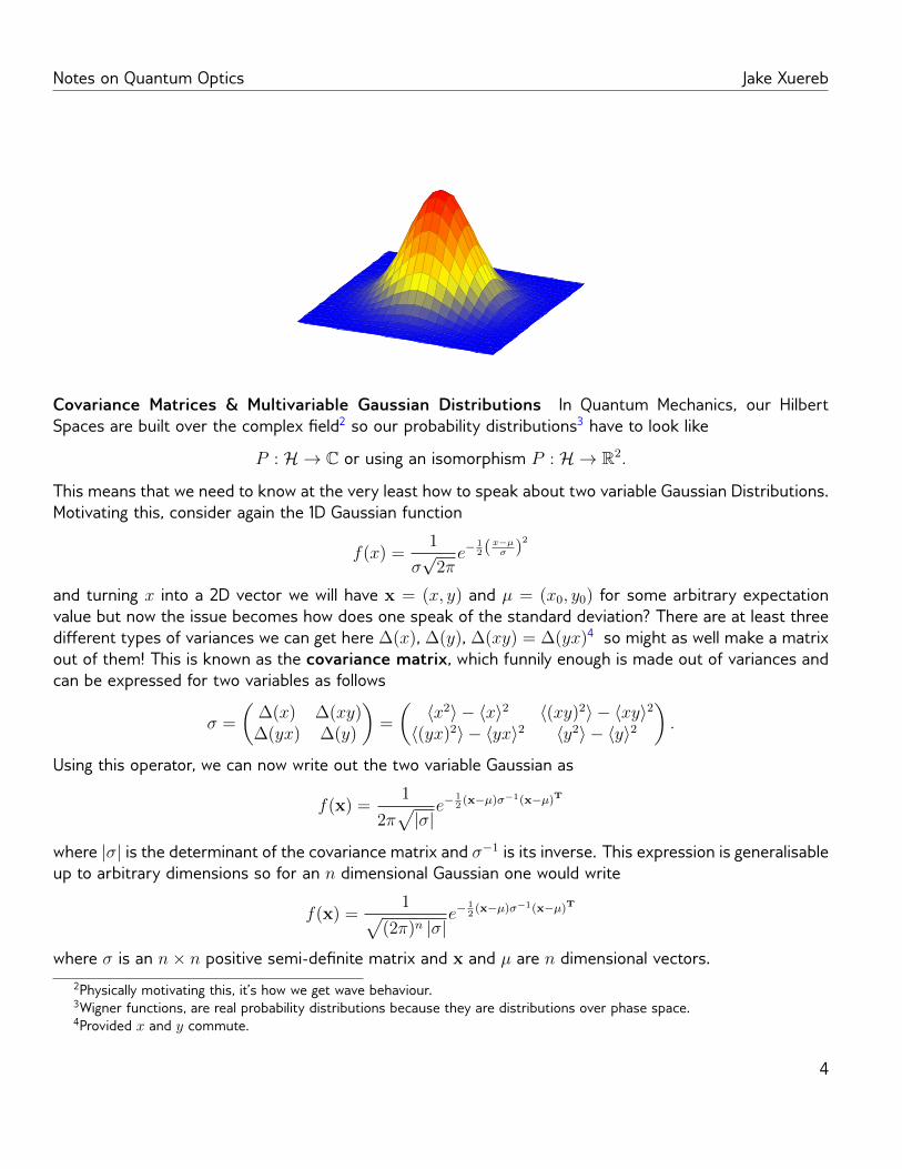
Covariance Matrices & Multivariable Gaussian Distributions In Quantum Mechanics, our HilbertSpaces are built over the complex eld2 so our probability distributions3 have to look like

P : H → C or using an isomorphism P : H → R2.

This means that we need to know at the very least how to speak about two variable Gaussian Distributions.Motivating this, consider again the 1D Gaussian function

f(x) =1

σ√

2πe−

12(x−µσ )

2

and turning x into a 2D vector we will have x = (x, y) and µ = (x0, y0) for some arbitrary expectationvalue but now the issue becomes how does one speak of the standard deviation? There are at least threedierent types of variances we can get here ∆(x), ∆(y), ∆(xy) = ∆(yx)4 so might as well make a matrixout of them! This is known as the covariance matrix, which funnily enough is made out of variances andcan be expressed for two variables as follows

σ =

(∆(x) ∆(xy)∆(yx) ∆(y)

)=

(〈x2〉 − 〈x〉2 〈(xy)2〉 − 〈xy〉2〈(yx)2〉 − 〈yx〉2 〈y2〉 − 〈y〉2

).

Using this operator, we can now write out the two variable Gaussian as

f(x) =1

2π√|σ|e−

12(x−µ)σ−1(x−µ)T

where |σ| is the determinant of the covariance matrix and σ−1 is its inverse. This expression is generalisableup to arbitrary dimensions so for an n dimensional Gaussian one would write

f(x) =1√

(2π)n |σ|e−

12(x−µ)σ−1(x−µ)T

where σ is an n× n positive semi-denite matrix and x and µ are n dimensional vectors.2Physically motivating this, it’s how we get wave behaviour.3Wigner functions, are real probability distributions because they are distributions over phase space.4Provided x and y commute.

4


The Gaussian Integral and Normalisation Consider the arbitrary Gaussian function g(x) = e−x2 . How

would one go about evaluating its integral over (−∞,∞)? Well, it’s possible to show this directly by methodsof analysis5 but there’s trick one can do to make this integral pliable using polar coordinates!Consider the integral ∫ ∞

−∞e−x

2

dx

the issue here is evidently the evaluation at the bounds but consider that this is just a positive number solet’s take its square root.

=

√∫ ∞−∞

e−x2 dx

√∫ ∞−∞

e−x2 dx

At this stage, x is just a dummy variable so let’s change one of them to y, giving two single variableGaussians

=

√∫ ∞−∞

e−y2 dx

√∫ ∞−∞

e−x2 dx =

√∫ ∞−∞

∫ ∞−∞

e−(x2+y2) dxdy

where I’ve used linearity of the integral operator and the distributivity of the square root over multiplication.Making use of polar coordinate we now are able to change the domain over which we are integrating fromx ∈ (−∞,∞) to r ∈ (0,∞), θ ∈ (0, 2π). This gives√∫ 2π

0

∫ ∞0

e−r2r drdθ

which is clearly a separable integral√∫ 2π

0

dθ

√∫ ∞0

e−r2r dr =√

2π

√∫ ∞0

e−r2r dr.

Focusing on the unevaluated integral let’s make a substitution of z = −r2 giving

√2π

√∫ 0

−∞e−zr

(−1

2r

)dz =

√2π

√[−ez

2

]0−∞

=√

2π

√[−e−r2

2

]∞0

=

√2π

(1

2

)and nally ∫ ∞

−∞e−x

2

dx =√π.

5https://math.stackexchange.com/questions/2703724/gaussian-integral-using-single-integration

5

https://math.stackexchange.com/questions/2703724/gaussian-integral-using-single-integration


Now that we known what the area under a Gaussian function is we can normalise it to make it a probabilitydistribution so consider the following Gaussian function with expectation value µ and variance σ2

f(x) = e−12(x−µσ )

and let’s compare it with a Gaussian function with z = x−µ√2σ

, that is

f(x) = e−12(x−µσ ) = e−z

2

.

The integral of e−z2 is clearly∫∞−∞ e

−z2dz =√π, as has been shown, so making use of z = x−µ√

2σwe have

by substitution ∫ ∞−∞

e−12(x−µσ )

(1

σ√

2

)dx =

∫ ∞−∞

e−z2

dz =√π

allowing us to write (1

σ√

2π

)∫ ∞−∞

e−12(x−µσ )dx = 1

deriving the normalisation factor.6

Moments The probability density is not the only way of describing a probability distribution. The mo-ments of a distribution are the expectation values of the distribution for dierent powers of x. So the n-thmoment would look like this

µn = 〈xn〉 =

∫ ∞−∞

xnf(x) dx.

These give information about the shape of the distribution and historically get their name from momentsof inertia in mechanics where the rst moment of a mass distribution is the center of mass and the secondmoment is the moment of inertia. Central moments are also used where the moment is shifted by theexpectation value

∫∞−∞(x− µ1)

nf(x) dx. Most notably, the variance is the second central moment∫ ∞−∞

(x− µ1)2f(x) dx

=

∫ ∞−∞

x2f(x)− 2xµ1f(x)− µ21f(x) dx

= 〈x2〉 − 2〈x〉2 + 〈x〉2

= 〈x2〉 − 〈x〉2 = ∆x.

These two moments are enough to uniquely determine Gaussian distributions7 and this fact will allow usto at times do away completely with probability densities and speak only of covariance matrices, but moreon this in pages to come.

6This proves∫∞−∞ e−

z2

a dz =√aπ as was asked in the appendix of the assignment.

7As it turns out, most well-known probability distributions may be described in such a way. Read more here.

6

https://math.stackexchange.com/questions/1377158/gaussian-distribution-determined-by-first-two-moments


For completeness, it is good to note the existence of moment-generating functions which are functionswhose n-th derivative will correspond to the n-th moment of some distribution and as such they arealternate way of speaking about a distribution. The radius of convergence of a moment-generating functiondetermines how many moments one needs to accurately speak of some distribution. This being said, themoment-generating function does not exist. When it does, it is the characteristic function, which alwaysexists.

Characteristic Functions The Characteristic function can be thought of as the Fourier Transform of theprobability density. To motivate this physically, consider that if I have a Gaussian distribution over position,then I will attain its characteristic function which will be a Gaussian function over momentum. It is evenmore remarkable that the derivatives of the characteristic function, give us the moments of the probabilitydistribution readily. That is, it is a moment-generating function. For these reasons it is ubiquitous to study.

ϕ(p) =

∫ ∞−∞

eipxf(x) dx = 〈eipx〉

Note that it is also expressible as a form of expectation value.

Operator Averages & Characteristics Functions for Operators The expectation value of an operatorwith respect to some distribution, which itself is an operator, can be expressed in terms of the traceoperation in the following way in terms of say the Fock basis, which I’ll introduce soon.

〈O〉 =∑i

ρi 〈i|O |i〉

=∑i,j

ρi 〈i|O|j〉〈j| |i〉

=∑i,j

ρi 〈j|i〉〈i|O |j〉

=∑i,j

〈j| ρi|i〉〈i|O |j〉

〈O〉 = tr(ρO)

This is sometimes referred to as an operator average. Making use of this expression and the idea that thecharacteristic function can be written in terms of a type of expectation value we are in position to promotethe characteristic function to operators over some distribution

ϕ(ξ) = 〈eixTΩξ〉 = tr(ρD(ξ))

where I have dened the Weyl Operator D(ξ) ≡ eixTΩξ and made use of a symplectic form8 which I will

introduce now.8One can see this as making sure the product of x and ξ respects the commutation relations.

7


1.2 Some results of Symplectic Geometry & Lie Algebra

Symplectic Forms & Transforms Quantum Mechanics in its phase space formulation, as we are dis-cussing within this note set, makes use of the idea of canonical quantisation where Poisson brackets arepromoted to commutators

f, g → [f ,g].

Now, Poisson brackets are symplectic invariants which is to say that they are artifacts of a larger structure,the same can be said of the commutator. These are both objects which satisfy the Jacobi Identity and formLie Algebras but I will bite my tongue and not speak further on this topic. A symplectic form is a bilinearform with the quality that

ω(x, y) = −ω(y, x)

by denition both the Poisson bracket and the commutator make use of symplectic forms. Being a bilinearform this also denes another type of inner/scalar product in this space which leads to invariants. Inparticular, with operators we may make use of the symplectic matrix dened as follows

Ω =n⊕i=1

(0 1−1 0

)= In ⊗ ω

So for a Hilbert Space H⊗n =⊗N

i=1H corresponding to N Bosonic modes which each have have a pair ofannihilation and creation operators, we can form vectors b ≡ (a1, a

†1, a2, a

†2 . . . , an, a

†n) which allow us to

write the Bosonic Commutation relations governing this space as

[bi,bj] = Ωi,j : i, j ∈ [2N ].

This also allows us to dene Symplectic Transformations in the following way

SΩST = Ω =⇒ S ∈ Sp(2n,F)

where S can be called a symplectic matrix/transform/operator and is an element of the symplectic groupover the eld F of size 2n, Sp(2n,F). The symplectic matrix is clearly itself a symplectic transform.

Williamson’s Theorem An operator M is said to be positive-denite operator if and only if all of itseigenvalues are positive. Take my word for it, symplectic matrices are able to diagonalise positive-denitematrices.

Theorem: Let M be a real positive-denite symmetric real 2n× 2n matrix.

There exists S ∈ Sp(2n,F) such that:

STMS =

[ν 00 ν

]with ν being a diagonal matrix of rank n. ν = diag(ν1, . . . , νn) is known as the symplectic spectrum ofM and involves the symplect eigenvalues of M which are invariant up to reordering under symplectictransformation. As such and making use of the fact that Ω = ΩT = Ω−1 ∈ Sp(2n,F) we can nd thesymplectic spectrum directly as follows

ν = Eig+(iΩM).

8


Baker-Campbell-Haussdorf Formula In a non-commutative algebra, it is not easy to nd an operatorZ which satises the following relationship given X and Y

eXeY = eZ.

The Baker-Campbell-Hausdor formula is the solution to this question giving us the following series

Z = X + Y + +Z +1

12[X, [X,Y]]− 1

12[Y, [X,Y]] . . .

which in some sense gives us an idea of how non-commutative this algebra is. In Quantum Mechanics, asa result of the canonical bosonic commutation relations our operators form part of the Heisenberg group,which has a commutativity that reduces this formula in the following way

eXeY = eX+Y+12[X,Y].

9


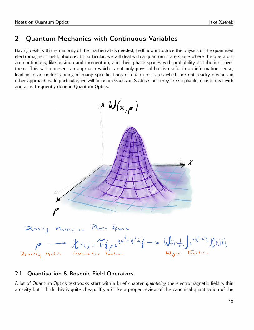
2 Quantum Mechanics with Continuous-VariablesHaving dealt with the majority of the mathematics needed, I will now introduce the physics of the quantisedelectromagnetic eld, photons. In particular, we will deal with a quantum state space where the operatorsare continuous, like position and momentum, and their phase spaces with probability distributions overthem. This will represent an approach which is not only physical but is useful in an information sense,leading to an understanding of many specications of quantum states which are not readily obvious inother approaches. In particular, we will focus on Gaussian States since they are so pliable, nice to deal withand as is frequently done in Quantum Optics.

2.1 Quantisation & Bosonic Field Operators

A lot of Quantum Optics textbooks start with a brief chapter quantising the electromagnetic eld withina cavity but I think this is quite cheap. If you’d like a proper review of the canonical quantisation of the

10


electromagnetic eld I recommend David Tong’s Notes on QFT. I will instead motivate the annihilation andcreation operators in a way which is more instructive via the harmonic oscillator and quantum harmonicoscillator which will serve as more than enough eld theory for us to move on to quantum optics withGaussian States.

The Harmonic Oscillator Sidney Coleman once remarked that ”The career of a young theoretical physicistconsists of treating the harmonic oscillator in ever-increasing levels of abstraction.”. Harmonic Oscillators havethe following equation of motion9

x+ ω20x = 0

where x is the coordinate of the oscillator and ω0 is the natural resonance frequency. This gives a Lagrangianof form

L =β

2x2 − 1

2αx2 ,

then applying the Euler-Lagrange equation gives

dLdx− d

dt

dLdx

= 0

x+1

αβx = 0 ,

which is correct for any α and β such that 1/αβ = ω20 .

Following the usual procedure to nd the Hamiltonian, we get

H =1

2αx2 +

1

2βp2

where the momentum p is dened as p ≡ ∂L∂q

= βx. Hamilton’s equations of motion are

p = −∂H∂q

=−xα

and q =∂H

∂p=p

β

or combined as a matrix equation

d

dt

[xp

]=

(0 1/β−1/α 0

)[xp

].

If we dene x ≡ Ax and y ≡ Bp with the constraint that A/B =√β/α, then our Hamilton equations of

motion becomed

dt

[xy

]= ω0

(0 1−1 0

)[xy

].

9Reference was made to https://physics.stackexchange.com/questions/432823/how-to-derive-annihilation-and-creation-operators

11

https://www.damtp.cam.ac.uk/user/tong/qft/qft.pdf

https://physics.stackexchange.com/questions/432823/how-to-derive-annihilation-and-creation-operators

https://physics.stackexchange.com/questions/432823/how-to-derive-annihilation-and-creation-operators


This is a set of rst order coupled dierential equations for x and y. To uncouple the equations, we solvefor the eigenvectors and eigenvalues of the matrix. They are

a ≡ x+ iy =

[1i

]with eigenvalue iω

and

a∗ ≡ x− iy =

[1−i

]with eigenvalue − iω .

Note that we have just found the eigenvalues of a symplectic matrix. These already look like the annihilationand creation operators, but let’s make this relationship more explicit.

The Quantum Harmonic Oscillator Consider again the Hamiltonian

H =p2

2m+mω2x2

2

with Poisson bracket x, p = 1 and promote this to a commutator [X, P ] = i~, respecting the uncertaintyrelations, where P = p√

mand X =

√mωx =

√k giving

H = P 2 + X2

where now, inspired by the expressions which diagonalised the classical hamiltonian one writes

H =

(X + iP

)√

2

(X − iP

)√

2+i

2

√k

m[P , X]

H =

(X + iP

)√

2

(X − iP

)√

2+

~ω2

and so denition of a hermitian conjugate follows

a ≡

(X − iP

)√

2~ωa† ≡

(X + iP

)√

2~ω

resulting in the Bosonic Commutation Relation [a, a†] = 1 and giving the diagonalised Hamiltonian as

H = ~ω(a†a+

1

2

).

These operators are known as the annihilation and creation operators respectively and the eigenspectrumof their product, the number operator, describes the energy levels of this quantum harmonic oscillator.

12


A State Space for the Quantised Electromagnetic Field The modes of the electromagnetic eld canbe written out in terms of our new friends the annihilation and creation operators. Making use of theCoulomb Gauge one arrives to the vector potential

A(r, t) =∑k

(~

2ωkε0

) 12 [akuk(r)e−iωkt + a†kuk

∗(r)eiωkt]

which is related to the magnetic and electric eld in the following ways

B = ∇×A E =−∂A

∂t.

The Hamiltonian of the electromagnetic eld is expressed as

H =1

2

∫ε0E

2 +1

µ0

B2dr

and expressing this Hamiltonian in terms of the gauge potential leads to

H =∑k

~ωk(ak†ak +

1

2

)where we recover the Hamiltonian of the quantum harmonic oscillator, indeed we have k of them eachrepresenting a mode of the electromagnetic eld. Using the Hamiltonian, one can derive an eigenbasis forthis space and we will do this shortly. Before this a mathematical look at this space shows a complex innerproduct space, a Hilbert Space, of innite dimension since the Hamiltonian oers a continuous spectrum.

If we have multiple such systems, say two photons, then we take the tensor product of the underlyingspaces to speak of them together. This means that for an n-dimensional quantum system we have h

H =n⊗i=1

Hi

13


where each of the composite spaces, is an innite dimensional Hilbert space in its own right, armed with itsown pair of creation and annihilation operators which observe the canonical Bosonic commutation relation

[ai, a†j] = δij.

This space is also armed with a non-trivial symplectic form (stemming from the promotion of the Poissonbrackets to commutators).Making use of the earlier denitions of the annihilation and creation operators we can express the quadra-ture phase operators, or position and momentum10 of each of these quantum harmonic oscillators in thefollowing way reversing the earlier derivation of these operators and setting dimensionless constants to 1.

xi =ai + a†i√

2pi =

ai + a†ii√

2

So as to speak of the quadratures of the whole space, the vector of operators R = (x1, p1, x2, p2, . . . , xn, pn)is introduced allowing us to write the canonical commutation relation observed by this space

[Rk,Rl] = iΩ

where Ω is the symplectic matrix introduced prior. And that’s . . . all the maths you need to live here.

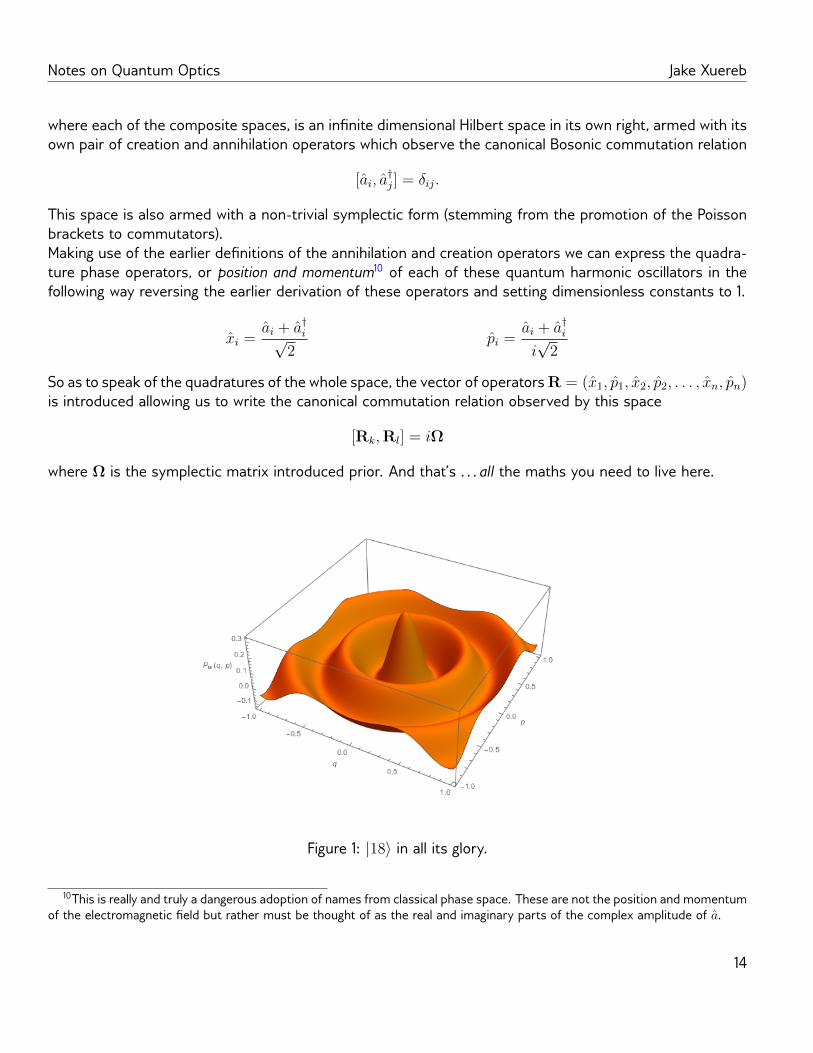
Figure 1: |18〉 in all its glory.

10This is really and truly a dangerous adoption of names from classical phase space. These are not the position and momentumof the electromagnetic eld but rather must be thought of as the real and imaginary parts of the complex amplitude of a.

14


2.2 A Zoo of States in Phase Space

Fock States By the Spectral Theorem we know that the eigenvectors of H provide a basis for the space.Clearly the eigenvectors of the number operator N = a†a are the eigenvectors of H and so provide a basisfor the Hilbert space of a mode. These states will satisfy the following relations with the number, creationand annihilation operators.

n |n〉 = a†a |n〉 = n |n〉 a |n〉 =√n |n− 1〉 a† |n〉 =

√n+ 1 |n+ 1〉 .

Since they form a basis in Hilbert Space, they are orthogonal and satisfy completeness

〈n|m〉 = δn,m

∞∑n=0

|n〉〈n| = 1.

For emphasis, say I have a 2D quantum state living in H = H1 ⊗H2, the basis states of this space wouldlook like |n〉1 ⊗ |m〉2. Physically, these states correspond directly to the energy levels of this quantumharmonic oscillator which is modeling our mode and conceptually are said to represent the number ofphotons occupying a mode, although I have my own philosophical qualms with this. We’ll examine themathematical form of these states in just a bit when we talk about characteristic functions.

Later we will compare the uncertainties in the quadratures of dierent states. Let’s nd the uncertaintyrelations for position and momentum for Fock states. Some things to note here are that ∆x = ∆p and

that the Heisenberg Uncertainty relation is observed for ~ = 1.

15


Displacement & Coherent States The complex form of the Weyl operator which was introduced earlieris the displacement operator. Conceptually, it is able to translate or displace states within the optical phasespace whilst mathematically it allows us to generate the eigenstates of the annihilation operator, known asthe coherent states.

D(α) ≡ eαa†−α∗a : α ∈ C

Making use of the Baker-Campbell-Haussdorf Formula, the Displacement operator can be written alterna-tively as follows

D(α) = e−−|α|2

2 eαa†e−α

∗a.

The Displacement operator lives up to its name aecting the creation and annihilation operators in thefollowing way

D†(α)aD(α) = a+ α D†(α)a†D(α) = a† + α∗.

Its most notable characteristic is that it generates coherent states from the vacuum state. The coherentstates are eigenstates of the annihilation operator.

|α〉 = D(α) |0〉 a |α〉 = α |α〉 .

Using all of this information we can now derive the uncertainty relations for coherent states. Evidently,

16


these states have an uncertainty which is the minimum possible and are in this vain as close to classicalas we can get within quantum optics. Another way to understand this is that these states are translatedvacuum states. The states being the spectrum of an operator of this space, the annihilation operator, forma basis form this space and thus satisfy completeness to the point that they form an overcomplete basis.

1 =1

2π

∫|α〉〈α| d2α

An inner product of a Fock state and a coherent state can be shown to observe

〈n|α〉 =αn

(n!)12

〈0|α〉 where 〈0|α〉 = 〈0| D(α) |0〉 = e−|α|2

2

〈n|α〉 =αn

(n!)12

e−|α|2

2

allowing us to write a direct relationship between the Fock basis and the Coherent basis as follows

|α〉 =∑n

|n〉〈n| |α〉 =∑n

|n〉〈n|α〉 =∑n

|n〉 αn

(n!)12

e−|α|2

2 .

The inner product between two coherent states can also be written explicitly using the Displacementoperator as

〈β|α〉 = 〈0| D†(β)D(α) |0〉 = e−12(|α|2+|β|2)+αβ∗

giving| 〈β|α〉 |2 = e−|α−β|

2

showing that the states become approximately orthogonal in the limit |α − β| >> 1 and explaining theovercompleteness of the basis.

Oh and nally and because I don’t want to mess up my gure placement, the displacement operator is aUnitary operator

D†(α) = D−1(α) = D(−α)

and using the Baker-Campbell-Haussdorf Formula we can write products of Displacement operators in thefollowing way

D(α)D(β) = e12(β∗α−α∗β)D(α + β).

17


Phase Space Just as in classical mechanics the notion of a phase space arises to encapsulate all thepossible states a system can occupy we can do this in quantum optics too. In particular, we are able tovisualise the uncertainty associated with an expectation value of some state. The Fock states and Coherentstates both clearly form circles in phase space as they have ∆x = ∆p. Soon we will see that squeezedstates form ellipses and that we can visualise and describe density matrices completely as distributionsover phase space using characteristic functions. This picture also allows us to clearly see the eect of the

displacement operator as the phase plot of a coherent state is clearly a displaced version of the phase plotof the vacuum state, as is evidenced by their uncertainty relations.

Squeezing in Phase Space Inspired by this picture, we could try to construct a minimum uncertaintystate, a state with the same uncertainty as a coherent state, but one where the quadratures do nothave equal uncertainty. Such states are known as squeezed states and are a general class of minimumuncertainty states which the coherent states can thought to be a specic class of squeezed states.

18


The Squeezing operator is dened as follows

S(ε) = e12ε∗a2− 1

2εa†

2

: ε = rei2φ

and transforms the annihilation and creation operators in the following way

S†(aa†

)S =

(a cosh r − a†ei2φ sinh ra† cosh r − ae−i2φ sinh r

).

It is a unitary operator satisfying the following relations

S†(ε) = S−1(ε) = S(−ε).

The eect of the squeezing operator on the two quadratures can be seen to be a rotation by e−iφ so

deningx′ + ip′ = (x+ ip) e−iφ

19


one is able to calculate11 the expectation values for the rotated quadratures as ∆x′ = 1√2e−r and ∆p′ = 1√

2er

allowing us to recover the minimum uncertainty relation

∆x′∆p′ =1

2.

Not that in this case ∆x′ 6= ∆p′. In fact we have the position quadrature being attenuated and themomentum quadrature being amplied (the example in the gure is reversed) giving us an ellipse in phasespace, a squeezed circle.

2.3 Charateristic Functions for Phase Space

We have seen that coherent states are quantum states which constitute a minimum uncertainty basis forquantum states of bosonic continuous variable quantum systems and that they form nice circles of radius12

in phase space, but these are not general states which we meet normally. Indeed, states can be formedas statistical ensembles of other states. Our prior education in quantum mechanics has armed us with atool known as density matrices for just a scenario but in a continuous variable system we can’t some overouter products we have to integrate

ρ =

∫P (α)|α〉〈α| d2α.

This P (α) is an unwieldy and tough density function to deal with directly. In such a case, it proves helpfulto take a page out of statistics and take a look at the characteristic function of this distribution and fromit attain the density function indirectly, since these quantities are related by a Fourier Transform.

The Characteristic function is expressed in terms of the Weyl Operator as

χ(ξ) = tr(ρD(ξ)) = tr(ρeixTΩξ)

where we have a function over ξ ∈ R2N . Let’s make this more explicit for a single mode state with phase

quadratures xT = (x, p) where Ω =

(0 1−1 0

)and we can take ξ =

(αβ

): α, β ∈ R.

ixTΩξ = i (βx− αp)

expanding in terms of annihilation and creation operators

=1√2

(−αa+ iβa+ αa† + iβa†

)where if we dene η = α+iβ√

2we get

ixTΩξ = ηa† − η∗a.which is what you’ll nd in Walls & Milburn. As such, the characteristic function can be written as

χ(η) = tr(ρeηa†−η∗a).

11These calculations are given in reasonable depth on pg.65 of Quantum Optics by Scully & Zubairy.

20


Now, looking at this characteristic function we see that we can have three dierent operator orderingssymmetric, normal and anti-normal ordering

χS(η) = tr(ρeηa†−η∗a) χN(η) = tr(ρeηa

†e−ηa

∗) χA(η) = tr(ρe−η

∗aeηa†)

giving three dierent density functions through an inverse Fourier transform.

W (α) =1

π2

∫eη∗α−ηα∗χS(η) d2η P (α) =

1

π2

∫eη∗α−ηα∗χN(η) d2η Q(α) =

1

π2

∫eη∗α−ηα∗χA(η) d2η

Respectively known as, the Wigner Function, the Glauber Sudarshan P-Function and the Husimi Q-Function.For this note set we’ll focus on Wigner functions.// Let’s do some examples!

The Wigner Function for a Coherent State The thing to keep in mind here is that since the char-acteristic function and the fourier transform term run over the same domain in the integral they mustbe evaluated together. Aside from this, complex numbers are split into their real and imaginary parts forevaluation of the integral and a standard integral is used.

21


Having found this expression we now take a look at what such a Wigner function looks like with the exampleof |5 + 3i〉 which gives

W (α) =2

πe−2|α−(5+3i)|2 =

2

πe−2((αr−5)

2+(αi−3)2)

This is clearly a Gaussian function and a proper probability distribution, giving even more credence to theidea that coherent states are as classical as we can get in continuous variable quantum mechanics.

Wigner Function for an ensemble of two coherent states We have the state ρ = 1N

(|α0〉〈α0|+ | − α0〉〈−α0|).Let’s normalise it, nd its Wigner function and plot it for an example coherent state ensemble withα = 5 + 3i. For normalisation, recall that density matrices have trace equal to 1 and observe the fol-lowing properties for operators

tr(A + B) = tr(A) + tr(B) tr(cA) = tr(A) + ctr(A)

allowing one to write

tr(ρ) = 1

tr(ρ) =1

N(tr|α0〉〈α0|+ tr| − α0〉〈−α0|) = 1

and since |±α0〉 is a pure state we have

(1 + 1) = N

and so

ρ =1

2(|α0〉〈α0|+ | − α0〉〈−α0|) .

22


Before considering the Wigner function as a whole, let’s consider the form of the characteristic function soas to be able to t it into the Wigner function in a way which is suitable. The Wigner function can be cal-culated now in the following way. So taking the example of ρ = 1

2(|5 + 3i〉〈5 + 3i|+ | − 5− 3i〉〈−5− 3i|)

we haveW (α) =

1

π

(e−2((αr−5)

2+(αi−3)2) + e−2((αr+5)2+(αi+3)2))

giving the following plot.

23


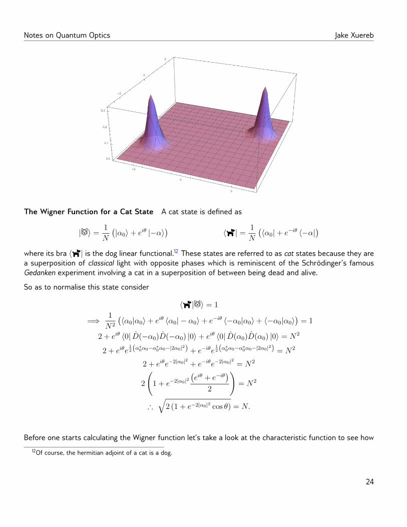
The Wigner Function for a Cat State A cat state is dened as

| 〉 =1

N

(|α0〉+ eiθ |−α〉

)〈| = 1

N

(〈α0|+ e−iθ 〈−α|

)where its bra 〈| is the dog linear functional.12 These states are referred to as cat states because they area superposition of classical light with opposite phases which is reminiscent of the Schrodinger’s famousGedanken experiment involving a cat in a superposition of between being dead and alive.

So as to normalise this state consider

〈| 〉 = 1

=⇒ 1

N2

(〈α0|α0〉+ eiθ 〈α0| − α0〉+ e−iθ 〈−α0|α0〉+ 〈−α0|α0〉

)= 1

2 + eiθ 〈0| D(−α0)D(−α0) |0〉+ eiθ 〈0| D(α0)D(α0) |0〉 = N2

2 + eiθe12(α∗0α0−α∗0α0−|2α0|2) + e−iθe

12(α∗0α0−α∗0α0−|2α0|2) = N2

2 + eiθe−2|α0|2 + e−iθe−2|α0|2 = N2

2

(1 + e−2|α0|2

(eiθ + e−iθ

)2

)= N2

∴√

2 (1 + e−2|α0|2 cos θ) = N.

Before one starts calculating the Wigner function let’s take a look at the characteristic function to see how12Of course, the hermitian adjoint of a cat is a dog.

24


to include it in the calculation. The density matrix for a cat state can be written as

ρ| 〉

=1

2 (1 + e−2|α0|2 cos θ)

(|α0〉〈α0|+ eiθ| − α0〉〈α0|+ e−iθ|α0〉〈−α0|+ | − α0〉〈−α0|

)Calculating the Wigner function we proceed as follows

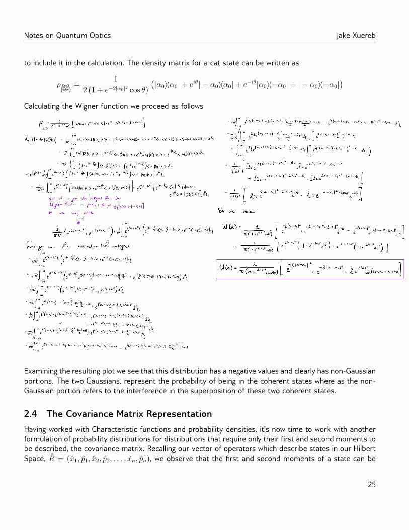
Examining the resulting plot we see that this distribution has a negative values and clearly has non-Gaussianportions. The two Gaussians, represent the probability of being in the coherent states where as the non-Gaussian portion refers to the interference in the superposition of these two coherent states.

2.4 The Covariance Matrix Representation

Having worked with Characteristic functions and probability densities, it’s now time to work with anotherformulation of probability distributions for distributions that require only their rst and second moments tobe described, the covariance matrix. Recalling our vector of operators which describe states in our HilbertSpace, R = (x1, p1, x2, p2, . . . , xn, pn), we observe that the rst and second moments of a state can be

25


Figure 2: The Wigner Function for a Cat State

given as a function of the expectation values of the vector of quadrature operators as

dj = 〈Rj〉ρ σij =1

2〈RiRj − RjRj〉ρ + 〈Ri〉ρ〈Rj〉ρ

respectively. As such for j = 1 we may write the covariance matrix as

σ(x, p) =

(〈x2〉 − 〈x〉2 1

2〈x, p〉 − 〈x〉〈p〉

12〈p, x〉 − 〈p〉〈x〉〈p2〉 − 〈p〉2

)which is real, symmetric and positive denite.

Now recalling what we learned in the rst section, covariance matrices can be used to formulate multivari-able probability densities and as such, we can write Gaussian Wigner Functions in terms of a covariancematrix in the following way

W (R) =1

π√|σ|e−(R−d)

T σ−1(R−d)

where d is the vector of rst moments.

For a coherent state we have d =√

2

[<(α0)=(α0)

]and σ = I clearly allowing one to recover

W (α) =2

πe−2|α−α0|2 .

Robertson-Schrodinger Uncertainty Relation

Entanglement with Gaussian States

The Lyapunov Equation

26

Documents

Notes on Quantum Optics - Jake Xuereb