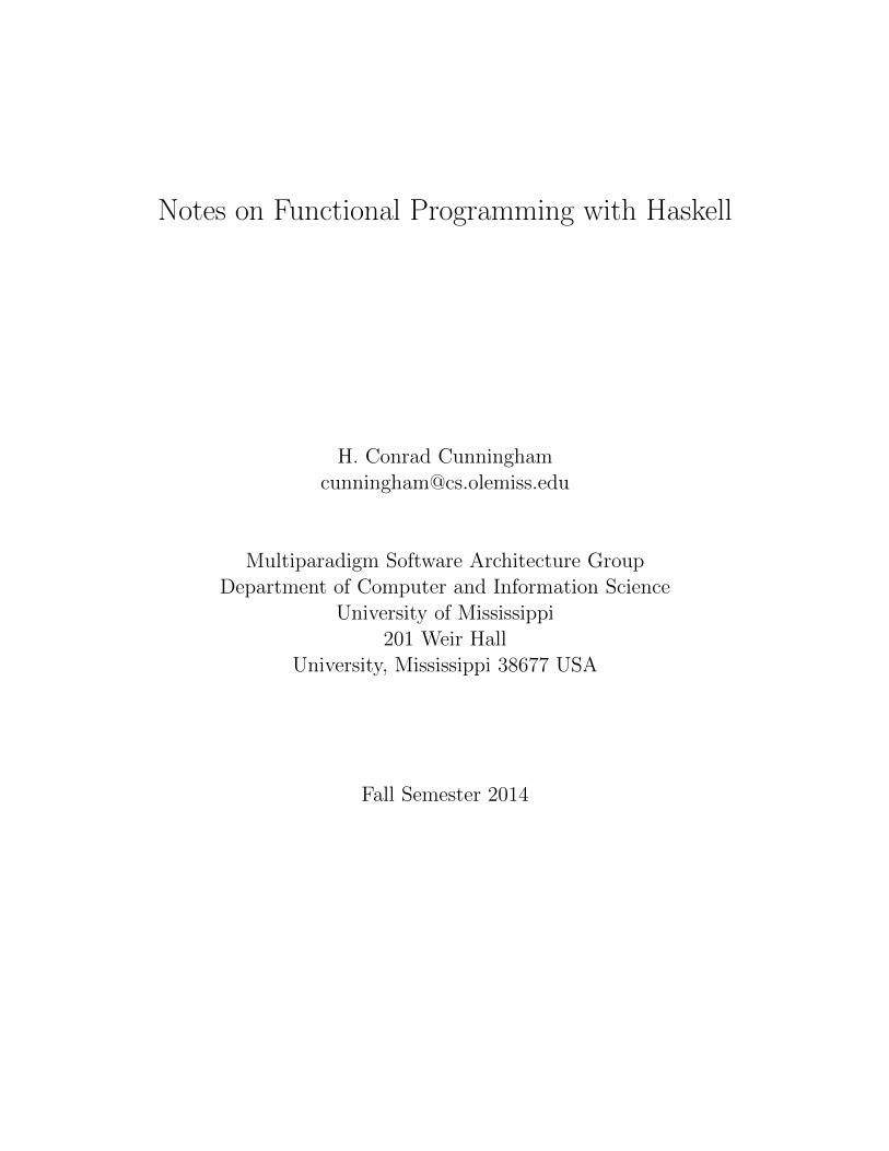
Notes on Functional Programming with Haskell

H. Conrad Cunninghamcunningham@cs.olemiss.edu

Multiparadigm Software Architecture GroupDepartment of Computer and Information Science

University of Mississippi201 Weir Hall

University, Mississippi 38677 USA

Fall Semester 2014

Copyright c© 1994, 1995, 1997, 2003, 2007, 2010, 2014 by H. Conrad Cunningham

Permission to copy and use this document for educational or research purposes ofa non-commercial nature is hereby granted provided that this copyright notice isretained on all copies. All other rights are reserved by the author.

H. Conrad Cunningham, D.Sc.Professor and ChairDepartment of Computer and Information ScienceUniversity of Mississippi201 Weir HallUniversity, Mississippi 38677USA

cunningham@cs.olemiss.edu

PREFACE TO 1995 EDITION

I wrote this set of lecture notes for use in the course Functional Programming (CSCI555) that I teach in the Department of Computer and Information Science at the Uni-versity of Mississippi. The course is open to advanced undergraduates and beginninggraduate students.

The first version of these notes were written as a part of my preparation for the fallsemester 1993 offering of the course. This version reflects some restructuring andrevision done for the fall 1994 offering of the course—or after completion of the class.For these classes, I used the following resources:

Textbook – Richard Bird and Philip Wadler. Introduction to Functional Program-ming, Prentice Hall International, 1988 [2].

These notes more or less cover the material from chapters 1 through 6 plusselected material from chapters 7 through 9.

Software – Gofer interpreter version 2.30 (2.28 in 1993) written by Mark P. Jones,available via anonymous FTP from directory pub/haskell/gofer at the Inter-net site nebula.cs.yale.edu.

Gofer is an interpreter for a dialect of the “lazy” functional programming lan-guage Haskell. This interpreter was available on both MS-DOS-based PC-compatibles, 486-based systems executing FreeBSD (“UNIX”), and other UNIXsystems.

Manual – Mark P. Jones. An Introduction to Gofer (Version 2.20), tutorial manualdistributed as a part of the Gofer system [15].

In addition to the Bird and Wadler textbook and the Gofer manual, I used thefollowing sources in the preparation of these lecture notes:

• Paul Hudak and Joseph H. Fasel. “A Gentle Introduction to Haskell”, ACMSIGPLAN NOTICES, Vol. 27, No. 5, May 1992 [12].

• Paul Hudak, Simon Peyton Jones, and Philip Wadler. “Report on the Pro-gramming Language Haskell: A Non-strict, Purely Functional Language”, ACMSIGPLAN NOTICES, Vol. 27, No. 5, May 1992 [13].

• E. P. Wentworth. Introduction to Functional Programming using RUFL, De-partment of Computer Science, Rhodes University, Grahamstown, South Africa,August 1990 [22].

This is a good tutorial and manual for the Rhodes University Functional Lan-guage (RUFL), a Haskell-like language developed by Wentworth. I used RUFLfor two previous offerings of my functional programming course, but switched to

iii

Gofer for the fall semester 1993 offering. My use this source was indirect—viamy handwritten lecture notes for the previous versions of the class.

• Paul Hudak. “Conception, Evolution, and Application of Functional Program-ming Languages”, ACM Computing Surveys , Vol. 21, No. 3, pages 359–411,September 1989 [11].

• Rob Hoogerwoord. The Design of Functional Programs: A Calculational Ap-proach, Doctoral Dissertation, Eindhoven Technical University, Eindhoven, TheNetherlands, 1989 [10].

• A. J. T. Davie An Introduction to Functional Programming Systems UsingHaskell, Cambridge University Press, 1992 [7].

• Anthony J. Field and Peter G. Harrison. Functional Programming, AddisonWesley, 1988 [8].

This book uses the “eager” functional language Hope.

• J. Hughes. “Why Functional Programming Matters,” The Computer Journal,Vol. 32, No. 2, pages 98–107, 1989 [14].

Although the Bird and Wadler textbook is excellent, I decided to supplement thebook with these notes for several reasons:

• I wanted to use Gofer/Haskell language concepts, terminology, and exampleprograms in my class presentations and homework exercises. Although closeto Haskell, the language in Bird and Wadler differs from Gofer and Haskellsomewhat in both syntax and semantics.

• Unlike the stated audience of the Bird and Wadler textbook, my students usu-ally have several years of experience in programming using traditional languageslike Pascal, C, or Fortran. This is both an advantage and a disadvantage. Onthe one hand, they have programming experience and programming languagefamiliarity on which I can build. On the other hand, they have an imperativemindset that sometimes is resistant to the declarative programming approach.I tried to take both into account as I drafted these notes.

• Because of a change in the language used from RUFL to Gofer, I needed torewrite my lecture notes in 1993 anyway. Thus I decided to invest a bit moreeffort and make them available in this form. (I expected about 25% more effort,but it probably took about 100% more effort. :-)

• The publisher of the Bird and Wadler textbook told me a few weeks before my1993 class began that the book would not be available until halfway throughthe semester. Fortunately, the books arrived much earlier than predicted. Inthe future, I hope that these notes will give me a “backup” should the book notbe available when I need it.

iv

Overall, I was reasonably satisfied with the 1993 draft of the notes. However, I didnot achieve all that I wanted. Unfortunately, other obligations did not allow meto substantially address these issues in the current revision. I hope to address thefollowing shortcomings in any future revision of the notes.

• I originally wanted the notes to introduce formal program proof and synthesisconcepts earlier and in a more integrated way than these notes currently do.But I did not have sufficient time to reorganize the course and develop the newmaterials needed. Also the desire to give nontrivial programming exercises ledme to focus on the language concepts and features and informal programmingtechniques during the first half of the course.

• Gofer/Haskell is a relatively large language with many features. In 1993 I spentmore time covering the language features than I initially planned to do. In the1994 class I reordered a few of the topics, but still spent more time on languagefeatures. For future classes I need to rethink the choice and ordering of thelanguage features presented. Perhaps a few of the language features should beomitted in an introductory course.

• Still yet there are a few important features that I did not cover. In particular, Idid not discuss the more sophisticated features of the type system in any detail(e.g., type classes, instances, and overloading).

• I did not cover all the material that I have in covered in one or both of theprevious versions of the course (e.g., cyclic structures, abstract data types, theeight queens problem, and applications of trees).

1997 Note: The 1997 revision is limited to the correction of a few errors. The springsemester 1997 class is using the new Hugs interpreter rather than Gofer and the text-book Haskell: The Craft of Functional Programming by Simon Thompson (Addison-Wesley, 1996).

2014 Note: The 2014 revision seeks primarily to update these Notes to use Haskell2010 and the Haskell Platform (i.e., GHC and GHCi). The focus is on chapters3, 5, 6, 7, 8, and 10, which are being used in teaching a Haskell-based functionalprogramming module in CSci 450 (Organization of Programming Languages).

v

Acknowledgements

I thank the many students in the CSCI 555 classes who helped me find many typo-graphical and presentation errors in the working drafts of these notes. I also thankthose individuals at other institutions who have examined these notes and suggestedimprovements.

I thank Diana Cunningham, my wife, for being patient with all the late nights ofwork that writing these notes required.

The preparation of this document was supported by the National Science Foundationunder Grant CCR-9210342 and by the Department of Computer and InformationScience at the University of Mississippi.

vi

Contents

1 INTRODUCTION 1

1.1 Course Overview . . . . . . . . . . . . . . . . . . . . . . . . . . . . . 1

1.2 Excerpts from Backus’ 1977 Turing Award Address . . . . . . . . . . 2

1.3 Programming Language Paradigms . . . . . . . . . . . . . . . . . . . 5

1.4 Reasons for Studying Functional Programming . . . . . . . . . . . . . 6

1.5 Objections Raised Against Functional Programming . . . . . . . . . . 11

2 FUNCTIONS AND THEIR DEFINITIONS 13

2.1 Mathematical Concepts and Terminology . . . . . . . . . . . . . . . . 13

2.2 Function Definitions . . . . . . . . . . . . . . . . . . . . . . . . . . . 15

2.3 Mathematical Induction over Natural Numbers . . . . . . . . . . . . 15

3 FIRST LOOK AT HASKELL 17

4 USING THE INTERPRETER 23

5 HASKELL BASICS 25

5.1 Built-in Types . . . . . . . . . . . . . . . . . . . . . . . . . . . . . . . 25

5.2 Programming with List Patterns . . . . . . . . . . . . . . . . . . . . . 30

5.2.1 Summation of a list (sumlist) . . . . . . . . . . . . . . . . . . 30

5.2.2 Length of a list (length’) . . . . . . . . . . . . . . . . . . . . 32

5.2.3 Removing adjacent duplicates (remdups) . . . . . . . . . . . . 32

5.2.4 More example patterns . . . . . . . . . . . . . . . . . . . . . . 34

5.3 Infix Operations . . . . . . . . . . . . . . . . . . . . . . . . . . . . . . 35

5.4 Recursive Programming Styles . . . . . . . . . . . . . . . . . . . . . . 36

5.4.1 Appending lists (++) . . . . . . . . . . . . . . . . . . . . . . . 36

5.4.2 Reversing a list (rev) . . . . . . . . . . . . . . . . . . . . . . . 37

5.4.3 Recursion Terminology . . . . . . . . . . . . . . . . . . . . . . 38

5.4.4 Tail recursive reverse (reverse’) . . . . . . . . . . . . . . . . 39

vii

5.4.5 Local definitions (let and where) . . . . . . . . . . . . . . . . 40

5.4.6 Fibonacci numbers . . . . . . . . . . . . . . . . . . . . . . . . 41

5.5 More List Operations . . . . . . . . . . . . . . . . . . . . . . . . . . . 43

5.5.1 Element selection (!!) . . . . . . . . . . . . . . . . . . . . . . 43

5.5.2 List-breaking operations (take and drop) . . . . . . . . . . . . 43

5.5.3 List-combining operations (zip) . . . . . . . . . . . . . . . . . 44

5.6 Rational Arithmetic Package . . . . . . . . . . . . . . . . . . . . . . . 44

5.7 Exercises . . . . . . . . . . . . . . . . . . . . . . . . . . . . . . . . . . 48

6 HIGHER-ORDER FUNCTIONS 55

6.1 Maps . . . . . . . . . . . . . . . . . . . . . . . . . . . . . . . . . . . . 55

6.2 Filters . . . . . . . . . . . . . . . . . . . . . . . . . . . . . . . . . . . 57

6.3 Folds . . . . . . . . . . . . . . . . . . . . . . . . . . . . . . . . . . . . 58

6.4 Strictness . . . . . . . . . . . . . . . . . . . . . . . . . . . . . . . . . 61

6.5 Currying and Partial Application . . . . . . . . . . . . . . . . . . . . 62

6.6 Operator Sections . . . . . . . . . . . . . . . . . . . . . . . . . . . . . 64

6.7 Combinators . . . . . . . . . . . . . . . . . . . . . . . . . . . . . . . . 65

6.8 Functional Composition . . . . . . . . . . . . . . . . . . . . . . . . . 66

6.9 Lambda Expressions . . . . . . . . . . . . . . . . . . . . . . . . . . . 69

6.10 List-Breaking Operations . . . . . . . . . . . . . . . . . . . . . . . . . 69

6.11 List-Combining Operations . . . . . . . . . . . . . . . . . . . . . . . . 70

6.12 Rational Arithmetic Revisited . . . . . . . . . . . . . . . . . . . . . . 72

6.13 Cosequential Processing . . . . . . . . . . . . . . . . . . . . . . . . . 73

6.14 Exercises . . . . . . . . . . . . . . . . . . . . . . . . . . . . . . . . . . 76

7 MORE LIST NOTATION 79

7.1 Sequences . . . . . . . . . . . . . . . . . . . . . . . . . . . . . . . . . 79

7.2 List Comprehensions . . . . . . . . . . . . . . . . . . . . . . . . . . . 80

7.2.1 Example: Strings of spaces . . . . . . . . . . . . . . . . . . . . 81

7.2.2 Example: Prime number test . . . . . . . . . . . . . . . . . . 81

viii

7.2.3 Example: Squares of primes . . . . . . . . . . . . . . . . . . . 82

7.2.4 Example: Doubling positive elements . . . . . . . . . . . . . . 82

7.2.5 Example: Concatenate a list of lists of lists . . . . . . . . . . . 82

7.2.6 Example: First occurrence in a list . . . . . . . . . . . . . . . 83

7.3 Exercises . . . . . . . . . . . . . . . . . . . . . . . . . . . . . . . . . . 84

8 MORE ON DATA TYPES 85

8.1 User-Defined Types . . . . . . . . . . . . . . . . . . . . . . . . . . . . 85

8.2 Recursive Data Types . . . . . . . . . . . . . . . . . . . . . . . . . . 87

8.3 Exercises . . . . . . . . . . . . . . . . . . . . . . . . . . . . . . . . . . 90

9 INPUT/OUTPUT 103

10 PROBLEM SOLVING 105

10.1 Polya’s Insights . . . . . . . . . . . . . . . . . . . . . . . . . . . . . . 105

10.2 Problem-Solving Strategies . . . . . . . . . . . . . . . . . . . . . . . . 106

11 HASKELL “LAWS” 109

11.1 Stating and Proving Laws . . . . . . . . . . . . . . . . . . . . . . . . 109

11.2 Associativity of ++ . . . . . . . . . . . . . . . . . . . . . . . . . . . . 111

11.3 Identity Element for ++ . . . . . . . . . . . . . . . . . . . . . . . . . . 113

11.4 Relating length and ++ . . . . . . . . . . . . . . . . . . . . . . . . . 114

11.5 Relating take and drop . . . . . . . . . . . . . . . . . . . . . . . . . 115

11.6 Equivalence of Functions . . . . . . . . . . . . . . . . . . . . . . . . . 116

11.7 Exercises . . . . . . . . . . . . . . . . . . . . . . . . . . . . . . . . . . 119

12 PROGRAM SYNTHESIS 123

12.1 Fast Fibonacci Function . . . . . . . . . . . . . . . . . . . . . . . . . 123

12.2 Sequence of Fibonacci Numbers . . . . . . . . . . . . . . . . . . . . . 126

12.3 Synthesis of drop from take . . . . . . . . . . . . . . . . . . . . . . . 130

12.4 Tail Recursion Theorem . . . . . . . . . . . . . . . . . . . . . . . . . 132

ix

12.5 Finding Better Tail Recursive Algorithms . . . . . . . . . . . . . . . . 136

12.6 Text Processing Example . . . . . . . . . . . . . . . . . . . . . . . . . 139

12.6.1 Line processing . . . . . . . . . . . . . . . . . . . . . . . . . . 139

12.6.2 Word processing . . . . . . . . . . . . . . . . . . . . . . . . . 143

12.6.3 Paragraph processing . . . . . . . . . . . . . . . . . . . . . . . 144

12.6.4 Other text processing functions . . . . . . . . . . . . . . . . . 145

12.7 Exercises . . . . . . . . . . . . . . . . . . . . . . . . . . . . . . . . . . 147

13 MODELS OF REDUCTION 149

13.1 Efficiency . . . . . . . . . . . . . . . . . . . . . . . . . . . . . . . . . 149

13.2 Reduction . . . . . . . . . . . . . . . . . . . . . . . . . . . . . . . . . 150

13.3 Head Normal Form . . . . . . . . . . . . . . . . . . . . . . . . . . . . 160

13.4 Pattern Matching . . . . . . . . . . . . . . . . . . . . . . . . . . . . . 162

13.5 Reduction Order and Space . . . . . . . . . . . . . . . . . . . . . . . 164

13.6 Choosing a Fold . . . . . . . . . . . . . . . . . . . . . . . . . . . . . . 169

14 DIVIDE AND CONQUER ALGORITHMS 171

14.1 Overview . . . . . . . . . . . . . . . . . . . . . . . . . . . . . . . . . . 171

14.2 Divide and Conquer Fibonacci . . . . . . . . . . . . . . . . . . . . . . 173

14.3 Divide and Conquer Folding . . . . . . . . . . . . . . . . . . . . . . . 173

14.4 Minimum and Maximum of a List . . . . . . . . . . . . . . . . . . . . 175

15 INFINITE DATA STRUCTURES 177

15.1 Infinite Lists . . . . . . . . . . . . . . . . . . . . . . . . . . . . . . . . 177

15.2 Iterate . . . . . . . . . . . . . . . . . . . . . . . . . . . . . . . . . . . 178

15.3 Prime Numbers: Sieve of Eratosthenes . . . . . . . . . . . . . . . . . 179

x

1 INTRODUCTION

1.1 Course Overview

This is a course on functional programming.

As a course on programming, it emphasizes the analysis and solution of problems, thedevelopment of correct and efficient algorithms and data structures that embody thesolutions, and the expression of the algorithms and data structures in a form suitablefor processing by a computer. The focus is more on the human thought processesthan on the computer execution processes.

As a course on functional programming, it approaches programming as the construc-tion of definitions for (mathematical) functions and data structures. Functional pro-grams consist of expressions that use these definitions. The execution of a functionalprogram entails the evaluation of the expressions making up the program. Thusthe course’s focus is on problem solving techniques, algorithms, data structures, andprogramming notations appropriate for the functional approach.

This is not a course on functional programming languages. In particular, the coursedoes not undertake an in-depth study of the techniques for implementing functionallanguages on computers. The focus is on the concepts for programming, not on theinternal details of the technological artifact that executes the programs.

Of course, we want to be able to execute our functional programs on a computer and,moreover, to execute them efficiently. Thus we must become familiar with some con-crete programming language and use an implementation of that language to executeour programs. To be able to analyze program efficiency, we must also become familiarwith the basic techniques that are used to evaluate expressions. To be specific, thisclass will use a functional programming environment called GHC (Glasgow HaskellCompiler). GHC is distributed in a “batteries included” bundle called the the HaskellPlatform . (That is, it bundles GHC with commonly used libraries and tools.) Thelanguage accepted by GHC is the “lazy” functional programming language Haskell2010. A program processed by GHC evaluates expressions according to an executionmodel called graph reduction.

Being “practical” is not an overriding concern of this course. Although functionallanguages are increasing in importance, their use has not yet spread much beyondthe academic and industrial research laboratories. While a student may take a courseon C++ programming and then go out into industry and find a job in which theC++ knowledge and skills can be directly applied, this is not likely to occur with acourse on functional programming.

However, the fact that functional languages are not broadly used does not mean thatthis course is impractical. A few industrial applications are being developed usingvarious functional languages. Many of the techniques of functional programming

1

can also be applied in more traditional programming and scripting languages. Moreimportantly, any time programmers learn new approaches to problem solving andprogramming, they become better programmers. A course on functional programmingprovides a novel, interesting, and, probably at times, frustrating opportunity to learnmore about the nature of the programming task. Enjoy the semester!

1.2 Excerpts from Backus’ 1977 Turing Award Address

This subsection contains excerpts from computing pioneer John Backus’ 1977 ACMTuring Award Lecture published as article “Can Programming Be Liberated fromthe von Neumann Style? A Functional Style and Its Algebra of Programs [1]” (Com-munications of the ACM, Vol. 21, No. 8, pages 613–41, August 1978). Althoughfunctional languages like Lisp go back to the late 1950’s, Backus’s address did muchto stimulate research community’s interest in functional programming languages andfunctional programming.

——

Programming languages appear to be in trouble. Each successive language incorpo-rates, with little cleaning up, all the features of its predecessors plus a few more.Some languages have manuals exceeding 500 pages; others cram a complex descrip-tion into shorter manuals by using dense formalisms. . . . Each new language claimsnew and fashionable features, such as strong typing or structured control statements,but the plain fact is that few languages make programming sufficiently cheaper ormore reliable to justify the cost of producing and learning to use them.

Since large increases in size bring only small increases in power, smaller, more elegantlanguages such as Pascal continue to be popular. But there is a desperate need for apowerful methodology to help us think about programs, and no conventional languageeven begins to meet that need. In fact, conventional languages create unnecessaryconfusion in the way we think about programs. . . .

In order to understand the problems of conventional programming languages, wemust first examine their intellectual parent, the von Neumann computer. What is avon Neumann computer? When von Neumann and others conceived of it . . . [in the1940’s], it was an elegant, practical, and unifying idea that simplified a number ofengineering and programming problems that existed then. Although the conditionsthat produced its architecture have changed radically, we nevertheless still identifythe notion of “computer” with this . . . concept.

In its simplest form a von Neumann computer has three parts: a central process-ing unit (or CPU), a store, and a connecting tube that can transmit a single wordbetween the CPU and the store (and send an address to the store). I propose tocall this tube the von Neumann bottleneck. The task of a program is to change the

2

contents of the store in some major way; when one considers that this task mustbe accomplished entirely by pumping single words back and forth through the vonNeumann bottleneck, the reason for its name becomes clear.

Ironically, a large part of the traffic in the bottleneck is not useful data but merelynames of data, as well as operations and data used only to compute such names.Before a word can be sent through the tube its address must be in the CPU; henceit must either be sent through the tube from the store or be generated by some CPUoperation. If the address is sent form the store, then its address must either havebeen sent from the store or generated in the CPU, and so on. If, on the other hand,the address is generated in the CPU, it must either be generated by a fixed rule (e.g.,“add 1 to the program counter”) or by an instruction that was sent through the tube,in which case its address must have been sent, and so on.

Surely there must be a less primitive way of making big changes in the store than bypushing vast numbers of words back and forth through the von Neumann bottleneck.Not only is this tube a literal bottleneck for the data traffic of a problem, but, moreimportantly, it is an intellectual bottleneck that has kept us tied to word-at-a-timethinking instead of encouraging us to think in terms of the larger conceptual units ofthe task at hand. . . .

Conventional programming languages are basically high level, complex versions of thevon Neumann computer. Our . . . old belief that there is only one kind of computeris the basis our our belief that there is only one kind of programming language, theconventional—von Neumann—language. The differences between Fortran and Algol68, although considerable, are less significant than the fact that both are based on theprogramming style of the von Neumann computer. Although I refer to conventionallanguages as “von Neumann languages” to take note of their origin and style, I donot, of course, blame the great mathematician for their complexity. In fact, somemight say that I bear some responsibility for that problem. [Note: Backus was oneof the designers of Fortran and of Algol-60.]

Von Neumann programming languages use variables to imitate the computer’s storagecells; control statements elaborate its jump and test instructions; and assignmentstatements imitate its fetching, storing, and arithmetic. The assignment statementis the von Neumann bottleneck of programming languages and keeps us thinking inword-at-at-time terms in much the same way the computer’s bottleneck does.

Consider a typical program; at its center are a number of assignment statementscontaining some subscripted variables. Each assignment statement produces a one-word result. The program must cause these statements to be executed many times,while altering subscript values, in order to make the desired overall change in thestore, since it must be done one word at a time. The programmer is thus concernedwith the flow of words through the assignment bottleneck as he designs the nest ofcontrol statements to cause the necessary repetitions.

3

Moreover, the assignment statement splits programming into two worlds. The firstworld comprises the right sides of assignment statements. This is an orderly world ofexpressions, a world that has useful algebraic properties (except that those propertiesare often destroyed by side effects). It is the world in which most useful computationtakes place.

The second world of conventional programming languages is the world of statements.The primary statement in that world is the assignment statement itself. All the otherstatements in the language exist in order to make it possible to perform a computationthat must be based on this primitive construct: the assignment statement.

This world of statements is a disorderly one, with few useful mathematical properties.Structured programming can be seen as a modest effort to introduce some order intothis chaotic world, but it accomplishes little in attacking the fundamental problemscreated by the word-at-a-time von Neumann style of programming, with its primitiveuse of loops, subscripts, and branching flow of control.

Our fixation on von Neumann languages has continued the primacy of the von Neu-mann computer, and our dependency on it has made non-von Neumann languagesuneconomical and has limited their development. The absence of full scale, effectiveprogramming styles founded on non-von Neumann principles has deprived designersof an intellectual foundation for new computer architectures. . . .

——

Note: In his Turing Award Address, Backus went on to describe FP, his proposalfor a functional programming language. He argued that languages like FP wouldallow programmers to break out of the von Neumann bottleneck and find new waysof thinking about programming. Although languages like Lisp had been in existencesince the late 1950’s, the widespread attention given to Backus’ address and paperstimulated new interest in functional programming to develop by researchers aroundthe world.

Aside: Above Backus states that “the world of statements is a disorderly one, withfew mathematical properties”. Even in 1977 this was a bit overstated since Dijkstra’swork on the weakest precondition calculus and other work on axiomatic semanticshad already appeared. However, because of the referential transparency (discussedlater) property of purely functional languages, reasoning can often be done in anequational manner within the context of the language itself. In contrast, the wp-calculus and other axiomatic semantic approaches must project the problem fromthe world of programming language statements into the world of predicate calculus,which is much more orderly.

4

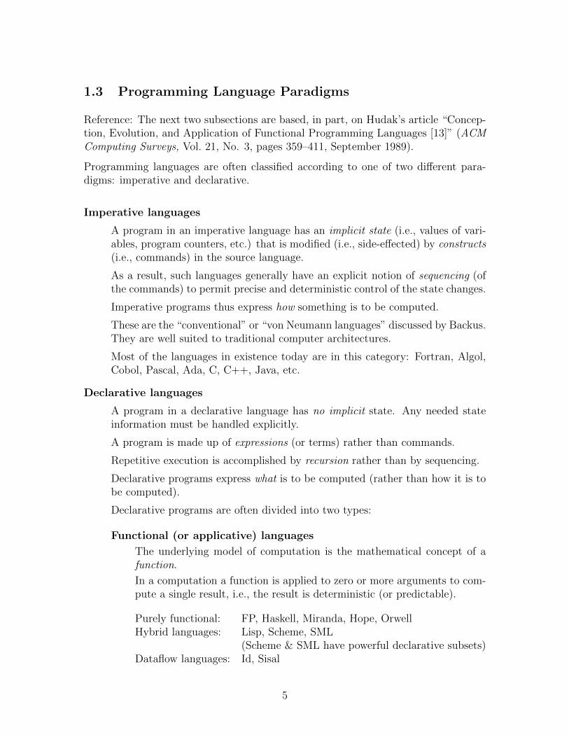
1.3 Programming Language Paradigms

Reference: The next two subsections are based, in part, on Hudak’s article “Concep-tion, Evolution, and Application of Functional Programming Languages [13]” (ACMComputing Surveys, Vol. 21, No. 3, pages 359–411, September 1989).

Programming languages are often classified according to one of two different para-digms: imperative and declarative.

Imperative languages

A program in an imperative language has an implicit state (i.e., values of vari-ables, program counters, etc.) that is modified (i.e., side-effected) by constructs(i.e., commands) in the source language.

As a result, such languages generally have an explicit notion of sequencing (ofthe commands) to permit precise and deterministic control of the state changes.

Imperative programs thus express how something is to be computed.

These are the “conventional” or “von Neumann languages” discussed by Backus.They are well suited to traditional computer architectures.

Most of the languages in existence today are in this category: Fortran, Algol,Cobol, Pascal, Ada, C, C++, Java, etc.

Declarative languages

A program in a declarative language has no implicit state. Any needed stateinformation must be handled explicitly.

A program is made up of expressions (or terms) rather than commands.

Repetitive execution is accomplished by recursion rather than by sequencing.

Declarative programs express what is to be computed (rather than how it is tobe computed).

Declarative programs are often divided into two types:

Functional (or applicative) languages

The underlying model of computation is the mathematical concept of afunction.

In a computation a function is applied to zero or more arguments to com-pute a single result, i.e., the result is deterministic (or predictable).

Purely functional: FP, Haskell, Miranda, Hope, OrwellHybrid languages: Lisp, Scheme, SML

(Scheme & SML have powerful declarative subsets)Dataflow languages: Id, Sisal

5

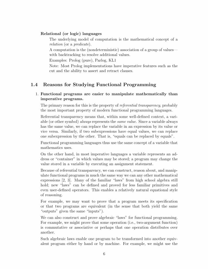
Relational (or logic) languages

The underlying model of computation is the mathematical concept of arelation (or a predicate).

A computation is the (nondeterministic) association of a group of values—with backtracking to resolve additional values.

Examples: Prolog (pure), Parlog, KL1

Note: Most Prolog implementations have imperative features such as thecut and the ability to assert and retract clauses.

1.4 Reasons for Studying Functional Programming

1. Functional programs are easier to manipulate mathematically thanimperative programs.

The primary reason for this is the property of referential transparency, probablythe most important property of modern functional programming languages.

Referential transparency means that, within some well-defined context, a vari-able (or other symbol) always represents the same value. Since a variable alwayshas the same value, we can replace the variable in an expression by its value orvice versa. Similarly, if two subexpressions have equal values, we can replaceone subexpression by the other. That is, “equals can be replaced by equals”.

Functional programming languages thus use the same concept of a variable thatmathematics uses.

On the other hand, in most imperative languages a variable represents an ad-dress or “container” in which values may be stored; a program may change thevalue stored in a variable by executing an assignment statement.

Because of referential transparency, we can construct, reason about, and manip-ulate functional programs in much the same way we can any other mathematicalexpressions [2, 3]. Many of the familiar “laws” from high school algebra stillhold; new “laws” can be defined and proved for less familiar primitives andeven user-defined operators. This enables a relatively natural equational styleof reasoning.

For example, we may want to prove that a program meets its specificationor that two programs are equivalent (in the sense that both yield the same“outputs” given the same “inputs”).

We can also construct and prove algebraic “laws” for functional programming.For example, we might prove that some operation (i.e., two-argument function)is commutative or associative or perhaps that one operation distributes overanother.

Such algebraic laws enable one program to be transformed into another equiv-alent program either by hand or by machine. For example, we might use the

6

laws to transform one program into an equivalent program that can be executedmore efficiently.

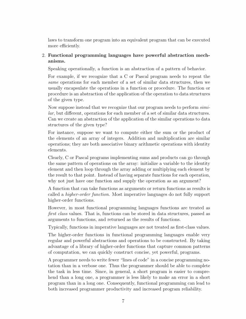
2. Functional programming languages have powerful abstraction mech-anisms.

Speaking operationally, a function is an abstraction of a pattern of behavior.

For example, if we recognize that a C or Pascal program needs to repeat thesame operations for each member of a set of similar data structures, then weusually encapsulate the operations in a function or procedure. The function orprocedure is an abstraction of the application of the operation to data structuresof the given type.

Now suppose instead that we recognize that our program needs to perform simi-lar, but different, operations for each member of a set of similar data structures.Can we create an abstraction of the application of the similar operations to datastructures of the given type?

For instance, suppose we want to compute either the sum or the product ofthe elements of an array of integers. Addition and multiplication are similaroperations; they are both associative binary arithmetic operations with identityelements.

Clearly, C or Pascal programs implementing sums and products can go throughthe same pattern of operations on the array: initialize a variable to the identityelement and then loop through the array adding or multiplying each element bythe result to that point. Instead of having separate functions for each operation,why not just have one function and supply the operation as an argument?

A function that can take functions as arguments or return functions as results iscalled a higher-order function. Most imperative languages do not fully supporthigher-order functions.

However, in most functional programming languages functions are treated asfirst class values. That is, functions can be stored in data structures, passed asarguments to functions, and returned as the results of functions.

Typically, functions in imperative languages are not treated as first-class values.

The higher-order functions in functional programming languages enable veryregular and powerful abstractions and operations to be constructed. By takingadvantage of a library of higher-order functions that capture common patternsof computation, we can quickly construct concise, yet powerful, programs.

A programmer needs to write fewer “lines of code” in a concise programming no-tation than in a verbose one. Thus the programmer should be able to completethe task in less time. Since, in general, a short program is easier to compre-hend than a long one, a programmer is less likely to make an error in a shortprogram than in a long one. Consequently, functional programming can lead toboth increased programmer productivity and increased program reliability.

7

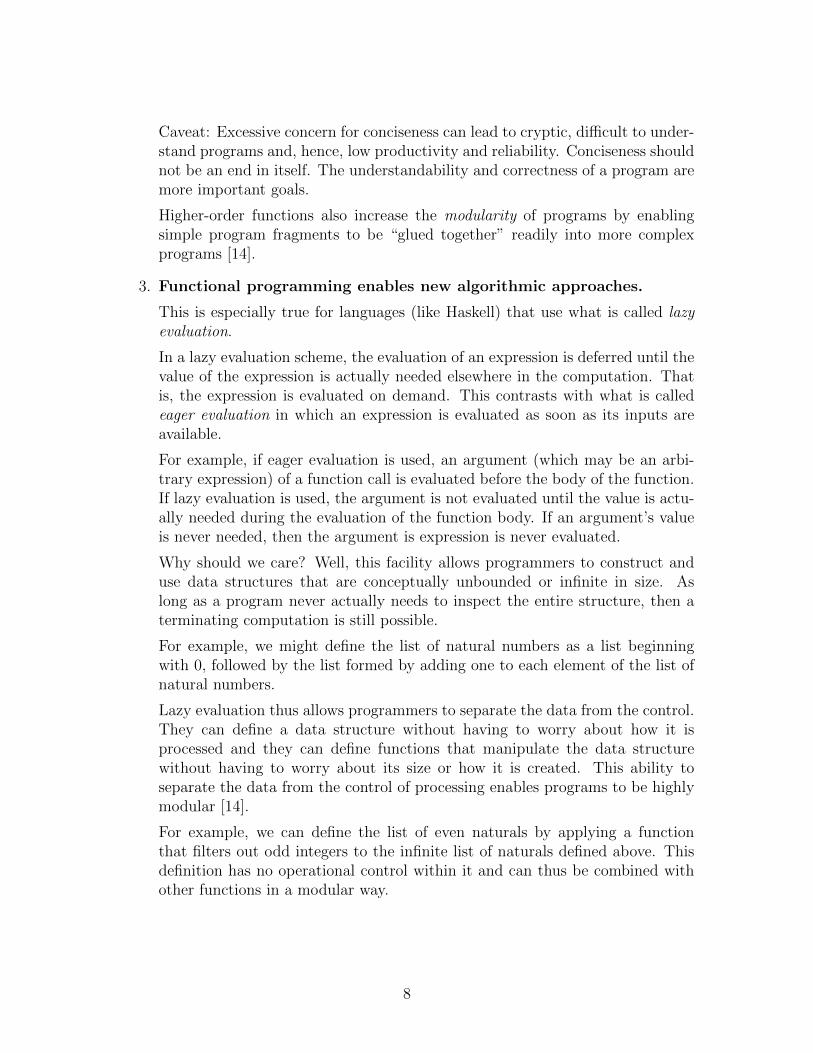
Caveat: Excessive concern for conciseness can lead to cryptic, difficult to under-stand programs and, hence, low productivity and reliability. Conciseness shouldnot be an end in itself. The understandability and correctness of a program aremore important goals.

Higher-order functions also increase the modularity of programs by enablingsimple program fragments to be “glued together” readily into more complexprograms [14].

3. Functional programming enables new algorithmic approaches.

This is especially true for languages (like Haskell) that use what is called lazyevaluation.

In a lazy evaluation scheme, the evaluation of an expression is deferred until thevalue of the expression is actually needed elsewhere in the computation. Thatis, the expression is evaluated on demand. This contrasts with what is calledeager evaluation in which an expression is evaluated as soon as its inputs areavailable.

For example, if eager evaluation is used, an argument (which may be an arbi-trary expression) of a function call is evaluated before the body of the function.If lazy evaluation is used, the argument is not evaluated until the value is actu-ally needed during the evaluation of the function body. If an argument’s valueis never needed, then the argument is expression is never evaluated.

Why should we care? Well, this facility allows programmers to construct anduse data structures that are conceptually unbounded or infinite in size. Aslong as a program never actually needs to inspect the entire structure, then aterminating computation is still possible.

For example, we might define the list of natural numbers as a list beginningwith 0, followed by the list formed by adding one to each element of the list ofnatural numbers.

Lazy evaluation thus allows programmers to separate the data from the control.They can define a data structure without having to worry about how it isprocessed and they can define functions that manipulate the data structurewithout having to worry about its size or how it is created. This ability toseparate the data from the control of processing enables programs to be highlymodular [14].

For example, we can define the list of even naturals by applying a functionthat filters out odd integers to the infinite list of naturals defined above. Thisdefinition has no operational control within it and can thus be combined withother functions in a modular way.

8

4. Functional programming enables new approaches to program devel-opment.

As we discussed above, it is generally easier to reason about functional programsthan imperative programs. It is possible to prove algebraic “laws” of functionalprograms that give the relationships among various operators in the language.We can use these laws to transform one program to another equivalent one.

These mathematical properties also open up new ways to write programs.

Suppose we want a program to break up a string of text characters into lines.Section 4.3 of the Bird and Wadler textbook [2] and Section 12.6 of these notesshows a novel way to construct this program.

First, Bird and Wadler construct a program to do the opposite of what wewant—to combine lines into a string of text. This function is very easy towrite.

Next, taking advantage of the fact that this function is the inverse of the desiredfunction, they use the “laws” to manipulate this simple program to find itsinverse. The result is the program we want!

5. Functional programming languages encourage (massively) parallel ex-ecution.

To exploit a parallel processor, it must be possible to decompose a programinto components that can be executed in parallel, assign these components toprocessors, coordinate their execution by communicating data as needed amongthe processors, and reassemble the results of the computation.

Compared to traditional imperative programming languages, it is quite easyto execute components of a functional program in parallel [19]. Because ofthe referential transparency property and the lack of sequencing, there are notime dependencies in the evaluation of expressions; the final value is the sameregardless of which expression is evaluated first. The nesting of expressionswithin other expressions defines the data communication that must occur duringexecution.

Thus executing a functional program in parallel does not require the availabilityof a highly sophisticated compiler for the language.

However, a more sophisticated compiler can take advantage of the algebraiclaws of the language to transform a program to an equivalent program that canmore efficiently be executed in parallel.

In addition, frequently used operations in the functional programming librarycan be be optimized for highly efficient parallel execution.

Of course, compilers can also be used to decompose traditional imperative lan-guages for parallel execution. But it is not easy to find all the potential par-allelism. A “smart” compiler must be used to identify unnecessary sequencingand find a safe way to remove it.

9

In addition to the traditional imperative programming languages, imperativelanguages have also been developed especially for execution on a parallel com-puter. These languages shift some of the work of decomposition, coordination,and communication to the programmer.

A potential advantage of functional languages over parallel imperative languagesis that the functional programmer does not, in general, need to be concernedwith the specification and control of the parallelism.

In fact, functional languages probably have the problem of too much potentialparallelism. It is easy to figure out what can be executed in parallel, but it issometimes difficult to determine what components should actually be executedin parallel and how to allocate them to the available processors. Functionallanguages may be better suited to the massively parallel processors of the futurethan most present day parallel machines.

6. Functional programming is important in some application areas ofcomputer science.

The artificial intelligence (AI) research community has used languages such asLisp and Scheme since the 1960’s. Some AI applications have been commercial-ized during the past two decades.

Also a number of the specification, modeling, and rapid-prototyping languagesthat are appearing in the software engineering community have features thatare similar to functional languages.

7. Functional programming is related to computing science theory.

The study of functional programming and functional programming languagesprovides a good opportunity to learn concepts related to programming languagesemantics, type systems, complexity theory, and other issues of importance inthe theory of computing science.

8. Functional programming is an interesting and mind-expanding activ-ity for students of computer science!?

Functional programming requires the student to develop a different perspectiveon programming.

10

1.5 Objections Raised Against Functional Programming

1. Functional programming languages are inefficient toys!

This was definitely true in the early days of functional programming. Functionallanguages tended to execute slowly, require large amounts of memory, and havelimited capabilities.

However, research on implementation techniques has resulted in more efficientand powerful implementations today.

Although functional language implementations will probably continue to in-crease in efficiency, they likely will never become as efficient as the implemen-tations of imperative “von Neumann” languages are on traditional “von Neu-mann” architectures.

However, new computer architectures may allow functional programs to ex-ecute competitively with the imperative languages on today’s architectures.For example, computers based on the dataflow and graph reduction models ofcomputation are more suited to execute functional languages than imperativelanguages.

Also the ready availability of parallel computers may make functional languagesmore competitive because they more readily support parallelism than traditionalimperative languages.

Moreover, processor time and memory usage just aren’t as important concernsas they once were. Both fast processors and large memories have become rel-atively inexpensive and readily available. Now it is common to dedicate oneor more processors and several megabytes of memory to individual users ofworkstations and personal computers.

As a result, the community can now afford to dedicate considerable computerresources to improving programmer productivity and program reliability; theseare issues that functional programming may address better than imperativelanguages.

2. Functional programming languages are not (and cannot be) used inthe real world!

It is still true that functional programming languages are not used very widelyin industry. But, as we have argued above, the functional style is becoming moreimportant—especially as commercial AI applications have begun to appear.

If new architectures like the dataflow machines emerge into the marketplace,functional programming languages will become more important.

Although the functional programming community has solved many of the dif-ficulties in implementation and use of functional languages, more research isneeded on several issues of importance to the real world: on facilities for in-put/output, nondeterministic, realtime, parallel, and database programming.

11

More research is also needed in the development of algorithms for the functionalparadigm. The functional programming community has developed functionalversions of many algorithms that are as efficient, in terms of big-O complexity,as the imperative versions. But there are a few algorithms for which efficientfunctional versions have not yet been found.

3. Functional programming is awkward and unnatural!

Maybe. It might be the case that functional programming somehow runscounter to the way that normal human minds work—that only mental deviantscan ever become effective functional programmers. Of course, some peoplemight say that about programming and programmers in general.

However, it seems more likely that the awkwardness arises from the lack ofeducation and experience. If we spend many years studying and doing pro-gramming in the imperative style, then any significantly different approach willseem unnatural.

Let’s give the functional approach a fair chance.

12

2 FUNCTIONS AND THEIR DEFINITIONS

2.1 Mathematical Concepts and Terminology

In mathematics, a function is a mapping from a set A into a set B such that eachelement of A is mapped into a unique element of B. The set A (on which f is defined)is called the domain of f . The set of all elements of B mapped to elements of A byf is called the range (or codomain) of f , and is denoted by f(A).

If f is a function from A into B, then we write:

f : A→ B

We also write the equation f(a) = b to mean that the value (or result) from applyingfunction f to an element a ∈ A is an element b ∈ B.

A function f : A → B is one-to-one (or injective) if and only if distinct elements ofA are mapped to distinct elements of B. That is, f(a) = f(a′) if and only if a = a′.

A function f : A → B is onto (or surjective) if and only if, for every element b ∈ B,there is some element a ∈ A such that f(a) = b.

A function f : A→ B is a one-to-one correspondence (or bijection) if and only if f isone-to-one and onto.

Given functions f : A→ B and g : B → C, the composition of f and g, written g ◦ f ,is a function from A into C such that

(g ◦ f)(a) = g(f(a)).

A function f−1 : B → A is an inverse of f : A → B if and only if, for every a ∈ A,f−1(f(a)) = a.

An inverse exists for any one-to-one function.

If function f : A → B is a one-to-one correspondence, then there exists an inversefunction f−1 : B → A such that, for every a ∈ A, f−1(f(a)) = a and that, for everyb ∈ B, f(f−1(b)) = b. Hence, functions that are one-to-one correspondences are alsosaid to be invertible.

If a function f : A → B and A ⊆ A′, then we say that f is a partial function fromA′ to B and a total function from A to B. That is, there are some elements of A′ onwhich f may be undefined.

13

A function ⊕ : (A × A) → A is called a binary operation on A. We usually writebinary operations in infix form: a⊕a′. (In computing science, we often call a function⊕ : (A×B)→ C a binary operation as well.)

Let ⊕ be a binary operation on some set A and x, y, and z be elements of A.

• Operation ⊕ is associative if and only if (x⊕ y)⊕ z = x⊕ (y ⊕ z) for any x, y,and z.

• Operation ⊕ is commutative (also called symmetric) if and only if x⊕y = y⊕xfor any x and y.

• An element e of set A is a left identity of ⊕ if and only if e⊕ x = x for any x, aright identity if and only if x⊕ e = x, and an identity if and only if it is both aleft and a right identity. An identity of an operation is sometimes called a unitof the operation.

• An element z of set A is a left zero of ⊕ if and only if z ⊕ x = z for any x, aright zero if and only if x ⊕ z = z, and a zero if and only if it is both a rightand a left zero.

• If e is the identity of ⊕ and x⊕ y = e for some x and y, then x is a left inverseof y and y is a right inverse of x. Elements x and y are inverses of each otherif x⊕ y = e = y ⊕ x.

• If ⊕ is an associative operation, then ⊕ and A are said to form a semigroup.

• A semigroup that also has an identity element is called a monoid.

• If every element of a monoid has an inverse then the monoid is called a group.

• If a monoid or group is also commutative, then it is said to be Abelian.

14

2.2 Function Definitions

Note: Mathematicians usually refer to the positive integers as the natural numbers.Computing scientists usually include 0 in the set of natural numbers.

Consider the factorial function fact. This function can be defined in several ways.For any natural number, we might define fact with the equation

fact(n) = 1× 2× 3× · · · × n

or, more formally, using the product operator as

fact(n) =i=n∏i=1

i

or, in the notation that the instructor prefers, as

fact(n) = (Π i : 1 ≤ i ≤ n : i).

We note that fact(0) = 1, the identity element of the multiplication operation.

We can also define the factorial function with a recursive definition (or recurrencerelation) as follows:

fact ′(n) =

{1, if n = 0n× fact ′(n− 1), if n ≥ 1

It is, of course, easy to see that the recurrence relation definition is equivalent to theprevious definitions. But how can we prove it?

To prove that the above definitions of the factorial function are equivalent, we canuse mathematical induction over the natural numbers.

2.3 Mathematical Induction over Natural Numbers

To prove a proposition P (n) holds for any natural number n, one must show twothings:

Base case n = 0. That P (0) holds.

Inductive case n = m+1. That, if P (m) holds for some natural number m, thenP (m+1) also holds. (The P (m) assumption is called the induction hypothesis.)

15

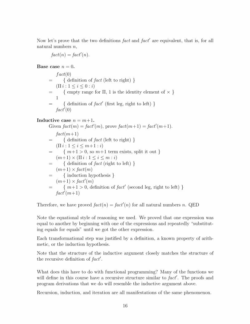
Now let’s prove that the two definitions fact and fact ′ are equivalent, that is, for allnatural numbers n,

fact(n) = fact ′(n).

Base case n = 0.

fact(0)= { definition of fact (left to right) }

(Π i : 1 ≤ i ≤ 0 : i)= { empty range for Π, 1 is the identity element of × }

1= { definition of fact ′ (first leg, right to left) }

fact ′(0)

Inductive case n = m+1.Given fact(m) = fact ′(m), prove fact(m+1) = fact ′(m+1).

fact(m+1)= { definition of fact (left to right) }

(Π i : 1 ≤ i ≤ m+1 : i)= { m+1 > 0, so m+1 term exists, split it out }

(m+1)× (Π i : 1 ≤ i ≤ m : i)= { definition of fact (right to left) }

(m+1)× fact(m)= { induction hypothesis }

(m+1)× fact ′(m)= { m+1 > 0, definition of fact ′ (second leg, right to left) }

fact ′(m+1)

Therefore, we have proved fact(n) = fact ′(n) for all natural numbers n. QED

Note the equational style of reasoning we used. We proved that one expression wasequal to another by beginning with one of the expressions and repeatedly “substitut-ing equals for equals” until we got the other expression.

Each transformational step was justified by a definition, a known property of arith-metic, or the induction hypothesis.

Note that the structure of the inductive argument closely matches the structure ofthe recursive definition of fact ′.

What does this have to do with functional programming? Many of the functions wewill define in this course have a recursive structure similar to fact ′. The proofs andprogram derivations that we do will resemble the inductive argument above.

Recursion, induction, and iteration are all manifestations of the same phenomenon.

16

3 FIRST LOOK AT HASKELL

Now let’s look at our first function definition in the Haskell language, a programto implement the factorial function for natural numbers. (For the purposes of thiscourse, remember that the natural numbers consist of 0 and the positive integers.)

In Section 2.2, we saw two definitions, fact and fact ′, that are equivalent for all naturalnumber arguments. We defined fact using the product operator as follows:

fact(n) =i=n∏i=1

i .

(We note that fact(0) = 1, which is the identity element of the multiplication opera-tion.)

We also defined the factorial function with a recursive definition (or recurrence rela-tion) as follows:

fact ′(n) =

{1, if n = 0n× fact ′(n− 1), if n ≥ 1

Since the domain of fact ′ is the set of natural numbers, a set over which induction isdefined, we can easily see that this recursive definition is well defined. For n = 0, thebase case, the value is simply 1. For n ≥ 1, the value of fact ′(n) is recursively definedin terms of fact ′(n − 1); the argument of the recursive application decreases towardthe base case.

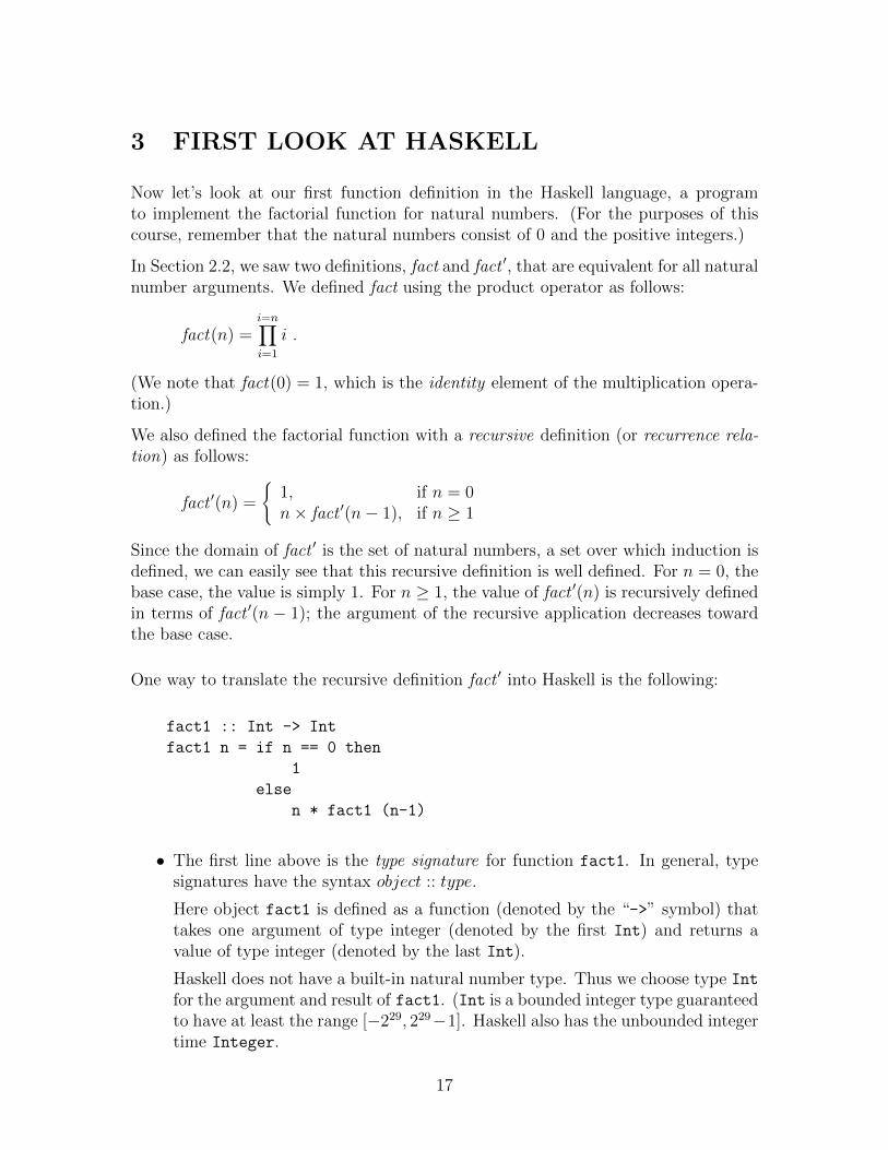
One way to translate the recursive definition fact ′ into Haskell is the following:

fact1 :: Int -> Int

fact1 n = if n == 0 then

1

else

n * fact1 (n-1)

• The first line above is the type signature for function fact1. In general, typesignatures have the syntax object :: type.

Here object fact1 is defined as a function (denoted by the “->” symbol) thattakes one argument of type integer (denoted by the first Int) and returns avalue of type integer (denoted by the last Int).

Haskell does not have a built-in natural number type. Thus we choose type Int

for the argument and result of fact1. (Int is a bounded integer type guaranteedto have at least the range [−229, 229−1]. Haskell also has the unbounded integertime Integer.

17

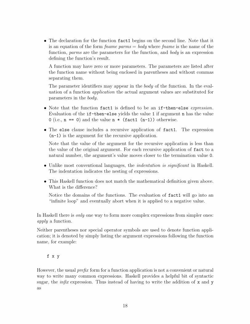
• The declaration for the function fact1 begins on the second line. Note that itis an equation of the form fname parms = body where fname is the name of thefunction, parms are the parameters for the function, and body is an expressiondefining the function’s result.

A function may have zero or more parameters. The parameters are listed afterthe function name without being enclosed in parentheses and without commasseparating them.

The parameter identifiers may appear in the body of the function. In the eval-uation of a function application the actual argument values are substituted forparameters in the body.

• Note that the function fact1 is defined to be an if-then-else expression.Evaluation of the if-then-else yields the value 1 if argument n has the value0 (i.e., n == 0) and the value n * (fact1 (n-1)) otherwise.

• The else clause includes a recursive application of fact1. The expression(n-1) is the argument for the recursive application.

Note that the value of the argument for the recursive application is less thanthe value of the original argument. For each recursive application of fact to anatural number, the argument’s value moves closer to the termination value 0.

• Unlike most conventional languages, the indentation is significant in Haskell.The indentation indicates the nesting of expressions.

• This Haskell function does not match the mathematical definition given above.What is the difference?

Notice the domains of the functions. The evaluation of fact1 will go into an“infinite loop” and eventually abort when it is applied to a negative value.

In Haskell there is only one way to form more complex expressions from simpler ones:apply a function.

Neither parentheses nor special operator symbols are used to denote function appli-cation; it is denoted by simply listing the argument expressions following the functionname, for example:

f x y

However, the usual prefix form for a function application is not a convenient or naturalway to write many common expressions. Haskell provides a helpful bit of syntacticsugar, the infix expression. Thus instead of having to write the addition of x and y

as

18

add x y

we can write it as

x + y

as we have since elementary school.

Function application (i.e., juxtaposition of function names and argument expressions)has higher precedence than other operators. Thus the expression f x + y is the sameas (f x) + y.

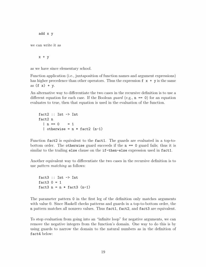
An alternative way to differentiate the two cases in the recursive definition is to use adifferent equation for each case. If the Boolean guard (e.g., n == 0) for an equationevaluates to true, then that equation is used in the evaluation of the function.

fact2 :: Int -> Int

fact2 n

| n == 0 = 1

| otherwise = n * fact2 (n-1)

Function fact2 is equivalent to the fact1. The guards are evaluated in a top-to-bottom order. The otherwise guard succeeds if the n == 0 guard fails; thus it issimilar to the trailing else clause on the if-then-else expression used in fact1.

Another equivalent way to differentiate the two cases in the recursive definition is touse pattern matching as follows:

fact3 :: Int -> Int

fact3 0 = 1

fact3 n = n * fact3 (n-1)

The parameter pattern 0 in the first leg of the definition only matches argumentswith value 0. Since Haskell checks patterns and guards in a top-to-bottom order, then pattern matches all nonzero values. Thus fact1, fact2, and fact3 are equivalent.

To stop evaluation from going into an “infinite loop” for negative arguments, we canremove the negative integers from the function’s domain. One way to do this is byusing guards to narrow the domain to the natural numbers as in the definition offact4 below:

19

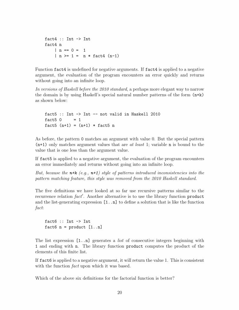
fact4 :: Int -> Int

fact4 n

| n == 0 = 1

| n >= 1 = n * fact4 (n-1)

Function fact4 is undefined for negative arguments. If fact4 is applied to a negativeargument, the evaluation of the program encounters an error quickly and returnswithout going into an infinite loop.

In versions of Haskell before the 2010 standard, a perhaps more elegant way to narrowthe domain is by using Haskell’s special natural number patterns of the form (n+k)

as shown below:

fact5 :: Int -> Int -- not valid in Haskell 2010

fact5 0 = 1

fact5 (n+1) = (n+1) * fact5 n

As before, the pattern 0 matches an argument with value 0. But the special pattern(n+1) only matches argument values that are at least 1; variable n is bound to thevalue that is one less than the argument value.

If fact5 is applied to a negative argument, the evaluation of the program encountersan error immediately and returns without going into an infinite loop.

But, because the n+k (e.g., n+1) style of patterns introduced inconsistencies into thepattern matching feature, this style was removed from the 2010 Haskell standard.

The five definitions we have looked at so far use recursive patterns similar to therecurrence relation fact ′. Another alternative is to use the library function product

and the list-generating expression [1..n] to define a solution that is like the functionfact:

fact6 :: Int -> Int

fact6 n = product [1..n]

The list expression [1..n] generates a list of consecutive integers beginning with1 and ending with n. The library function product computes the product of theelements of this finite list.

If fact6 is applied to a negative argument, it will return the value 1. This is consistentwith the function fact upon which it was based.

Which of the above six definitions for the factorial function is better?

20

Most people in the functional programming community would consider fact5 andfact6 as being better than the others. The choice between them depends uponwhether one wants to trap the application to negative numbers as an error or toreturn the value 1.

21

22

4 USING THE INTERPRETER

This section from the Gofer/Hugs Notes was obsolete. The course now uses theGlasgow Haskell Compiler (GHC) and its interactive interface GHCi. The authorremoved the text but left the section as a placeholder for a future revision.

23

24

5 HASKELL BASICS

5.1 Built-in Types

The type system is an important part of Haskell; the compiler or interpreter usesthe type information to detect errors in expressions and function definitions. To eachexpression Haskell assigns a type that describes the kind of value represented by theexpression.

Haskell has both built-in types and facilities for defining new types. In the followingwe discuss the built-in types. Note that a Haskell type name begins with a capitalletter.

Integers: Int and Integer

The Int data type is usually the integer data type supported directly by the hostprocessor (e.g., 32- or 64-bits on most current processors), but it is guaranteed tohave the range of at least a 30-bit, two’s complement integer. The type Integer isan unbounded precision integer type. Haskell supports the usual integer literals (i.e.,constants) and operations.

Floating point numbers: Float and Double

The Float and Double data types are the single and double precision floating pointnumbers on the host processor. Haskell floating point literals must include a decimalpoint; they may be signed or in scientific notation: 3.14159, 2.0, -2.0, 1.0e4,5.0e-2, -5.0e-2.

Booleans: Bool

Boolean literals are True and False (note capitals). Haskell supports Boolean oper-ations such as && (and), || (or), and not.

Characters: Char

Haskell uses Unicode for its character data type. Haskell supports character literalsenclosed in single quotes—including both the graphic characters (e.g., ’a’, ’0’, and’Z’) and special codes entered following the escape character backslash “\” (e.g.,’\n’ for newline, ’\t’ for horizontal tab, and ’\\’ for backslash itself).

25

In addition, a backslash character \ followed by a number generates the correspondingUnicode character code. If the first character following the backslash is o, then thenumber is in octal representation; if followed by x, then in hexadecimal notation; andotherwise in decimal notation.

For example, the exclamation point character can be represented in any of the fol-lowing ways: ’!’, ’\33’, ’\o41’, ’\x21’

Functions: t1 -> t2

If t1 and t2 are types then t1 -> t2 is the type of a function that takes an argumentof type t1 and returns a result of type t2. Function and variable names begin withlowercase letters optionally followed by a sequences of characters each of which is aletter, a digit, an apostrophe (′ ) (sometimes pronounced “prime”), or an underscore( ).

Haskell functions are first-class objects. They can be arguments or results of otherfunctions or be components of data structures. Multi-argument functions are curried–that is, treated as if they take their arguments one at a time.

For example, consider the integer addition operation (+). In mathematics, we nor-mally consider addition as an operation that takes a pair of integers and yields aninteger result, which would have the type signature

(+) :: (Int,Int) -> Int

In Haskell, we give the addition operation the type

(+) :: Int -> (Int -> Int)

or just

(+) :: Int -> Int -> Int

since -> binds from the right.

Thus (+) is a one argument function that takes some Int argument and returns afunction of type Int -> Int. Hence, the expression ((+) 5) denotes a function thattakes one argument and returns that argument plus 5.

We sometimes speak of this (+) operation as being partially applied (i.e., to oneargument instead of two).

This process of replacing a structured argument by a sequence of simpler ones is calledcurrying , named after American logician Haskell B. Curry who first described it.

26

The Haskell library, called the standard prelude, contains a wide range of predefinedfunctions including the usual arithmetic, relational, and Boolean operations. Someof these operations are predefined as infix operations.

Lists: [t]

The primary built-in data structure in Haskell is the list, a sequence of values. Allthe elements in a list must have the same type. Thus we declare lists with notationsuch as [t] to denote a list of zero or more elements of type t.

A list is is hierarchical data structure. It is either empty or it is a pair consisting ofa head element and a tail that is itself a list of elements.

Empty square brackets ([]), pronounced “nil”, represent the empty list.

A colon (:), pronounced “cons”, represents the list constructor operation between ahead element on the left and a tail list on the right.

For example, [], 2:[], and 3:(2:[]) denote lists.

Haskell adds a bit of syntactic sugar to make expressing lists easier. The cons op-erations binds from the right. Thus 5:(3:(2:[])) can be written 5:3:2:[]. As afurther convenience, a list can be written as a comma-separated sequence enclosed inbrackets, e.g., 5:3:2:[] as [5,3,2].

Haskell supports two list selector functions, head and tail, such that:

head (h:t) =⇒ h, where h is the head element of list,tail (h:t) =⇒ t, where t is the tail list.

Aside: Instead of head, Lisp uses car and other languages use hd, first, etc. Insteadof tail, Lisp uses cdr and other languages use tl, rest, etc.

The Prelude supports a number of other useful functions on lists. For example,length takes a list and returns its length.

Note that lists are defined inductively. That is, they are defined in terms of a baseelement [] and the list constructor operation cons (:). As you would expect, a form ofmathematical induction can be used to prove that list-manipulating functions satisfyvarious properties. We will discuss in Section 11.1.

Strings: String

In Haskell, a string is treated as a list of characters.. Thus the data type String isdefined with a type synonym as follows:

type String = [Char]

27

In addition to the standard list syntax, a String literal can be given by a sequenceof characters enclosed in double quotes. For example, "oxford" is shorthand for[’o’,’x’,’f’,’o’,’r’,’d’].

Strings can contain any graphic character or any special character given as escapecode sequence (using backslash). The special escape code \& is used to separate anycharacter sequences that are otherwise ambiguous.

Example: "Hello\nworld!\n" is a string that has two newline characters embedded.

Example: "\12\&3" represents the list [’\12’,’3’].

Because strings are represented as lists, all of the Prelude functions for manipulatinglists also apply to strings.

head "oxford" =⇒ ’o’

tail "oxford" =⇒ "xford"

Consider a function to compute the length of a string:

len :: String -> Int

len s = if s == [] then 0 else 1 + len (tail s)

Simulation (this is not necessarily the series of steps actually taken during executionof the Haskell program):

len "five"

=⇒ 1 + len (tail "five")

=⇒ 1 + len "ive"

=⇒ 1 + (1 + len (tail "ive"))

=⇒ 1 + (1 + len "ve")

=⇒ 1 + (1 + (1 + len (tail "ve")))

=⇒ 1 + (1 + (1 + len "e"))

=⇒ 1 + (1 + (1 + (1 + len (tail "e"))))

=⇒ 1 + (1 + (1 + (1 + len "")))

=⇒ 1 + (1 + (1 + (1 + 0)))

=⇒ 1 + (1 + (1 + 1))

=⇒ 1 + (1 + 2)

=⇒ 1 + 3

=⇒ 4

Note that the argument string for the recursive application of len is simpler (i.e.,shorter) than the original argument. Thus len will eventually be applied to a []

argument and, hence, len’s evaluation will terminate.

The above definition of len only works for strings. How can we make it work for alist of integers or other elements?

28

For an arbitrary type a, we want len to take objects of type [a] and return an Int

value. Thus its type signature could be:

len :: [a] -> Int

If a is a variable name (i.e., it begins with a lowercase letter) that does not alreadyhave a value, then the type expression a used as above is a type variable; it canrepresent an arbitrary type. All occurrences of a type variable appearing in a typesignature must, of course, represent the same type.

An object whose type includes one or more type variables can be thought of havingmany different types and is thus described as having a polymorphic type. (Literally,its type has “many shapes”.)

Polymorphism and first-class functions are powerful abstraction mechanisms: theyallow irrelevant detail to be hidden.

Examples of polymorphism include:

head :: [a] -> a

tail :: [a] -> [a]

(:) :: a -> [a] -> [a]

Tuples: (t1,t2,· · ·,tn)

If t1, t2, · · ·, tn are types, where n is finite and n ≥ 2, then (t1,t2,· · ·,tn) is atype consisting of n-tuples where the various components have the type given for thatposition.

Unlike lists, the elements in a tuple may have different types. Also unlike lists, thenumber of elements in a tuple is fixed. The tuple is analogous to the record in Pascalor structure in C.

Examples:

(1,[2],3) :: (Int, [Int], Int)

((’a’,False),(3,4)) :: ((Char, Bool), (Int, Int))

type Complex = (Float,Float)

makeComplex :: Float -> Float -> Complex

makeComplex r i = (r,i)

29

5.2 Programming with List Patterns

In the factorial examples we used integer and natural number patterns to break outvarious cases of a function definition into separate equations. Lists and other datatypes may also be used in patterns.

Pattern matching helps enable the form of the algorithm match the form of the datastructure.

This is considered elegant. It is also pragmatic. The structure of the data oftensuggests the algorithm that is needed for a task.

In general, lists have two cases that need to be handled: the empty list and thenonempty list. Breaking a definition for a list-processing function into these twocases is usually a good place to begin.

5.2.1 Summation of a list (sumlist)

Consider a function sumlist to sum all the elements in a list of integers. That is, ifthe list is v1, v2, v3, · · · , vn, then the sum of the list is the value resulting from insertingthe addition operator between consecutive elements of the list: v1 + v2 + v3 + · · ·+ vn.

Since addition is an associative operation (that is, (x + y) + z = x + (y + z) for anyintegers x, y, and z), the above additions can be computed in any order.

What is the sum of an empty list?

Since there are no numbers to add, then, intuitively, zero seems to be the propervalue for the sum.

In general, if some binary operation is inserted between the elements of a list, then theresult for an empty list is the identity element for the operation. Since 0+x = x = x+0for all integers x, zero is the identity element for addition.

Now, how can we compute the sum of a nonempty list?

Since a nonempty list has at least one element, we can remove one element and addit to the sum of the rest of the list. Note that the “rest of the list” is a simpler (i.e.,shorter) list than the original list. This suggests a recursive definition.

The fact that Haskell defines lists recursively as a cons of a head element with a taillist suggests that we structure the algorithm around the structure of the beginning ofthe list.

30

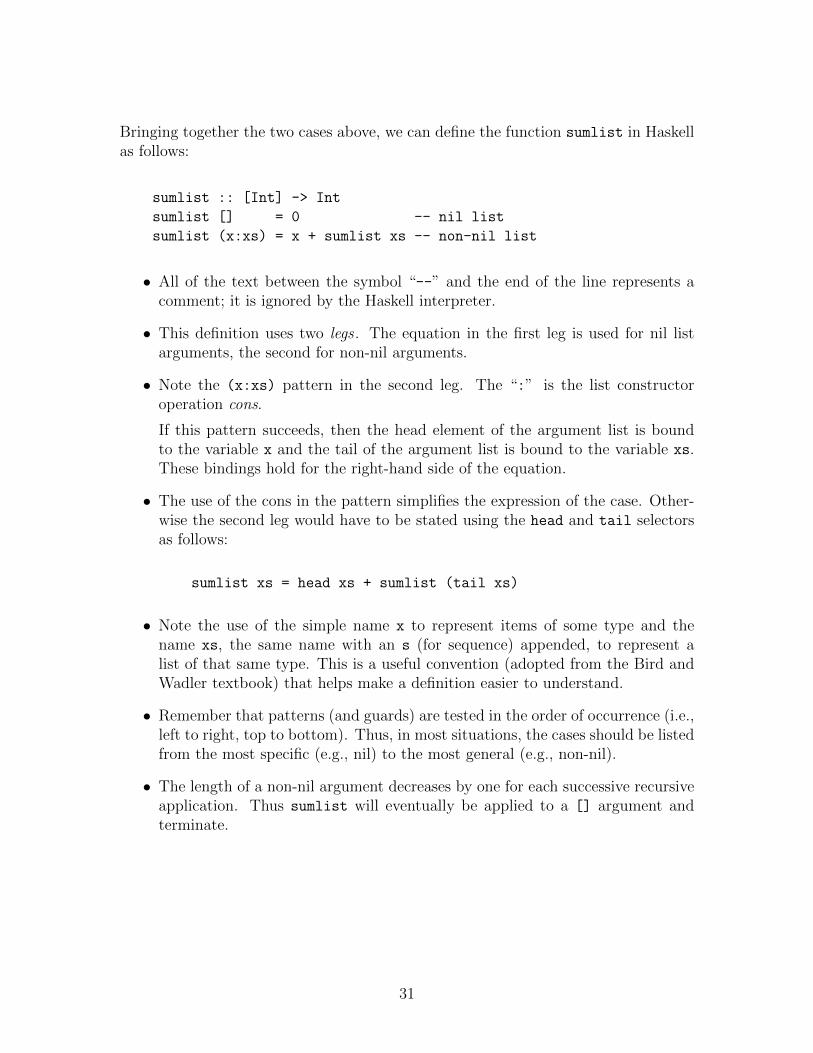
Bringing together the two cases above, we can define the function sumlist in Haskellas follows:

sumlist :: [Int] -> Int

sumlist [] = 0 -- nil list

sumlist (x:xs) = x + sumlist xs -- non-nil list

• All of the text between the symbol “--” and the end of the line represents acomment; it is ignored by the Haskell interpreter.

• This definition uses two legs . The equation in the first leg is used for nil listarguments, the second for non-nil arguments.

• Note the (x:xs) pattern in the second leg. The “:” is the list constructoroperation cons.

If this pattern succeeds, then the head element of the argument list is boundto the variable x and the tail of the argument list is bound to the variable xs.These bindings hold for the right-hand side of the equation.

• The use of the cons in the pattern simplifies the expression of the case. Other-wise the second leg would have to be stated using the head and tail selectorsas follows:

sumlist xs = head xs + sumlist (tail xs)

• Note the use of the simple name x to represent items of some type and thename xs, the same name with an s (for sequence) appended, to represent alist of that same type. This is a useful convention (adopted from the Bird andWadler textbook) that helps make a definition easier to understand.

• Remember that patterns (and guards) are tested in the order of occurrence (i.e.,left to right, top to bottom). Thus, in most situations, the cases should be listedfrom the most specific (e.g., nil) to the most general (e.g., non-nil).

• The length of a non-nil argument decreases by one for each successive recursiveapplication. Thus sumlist will eventually be applied to a [] argument andterminate.

31

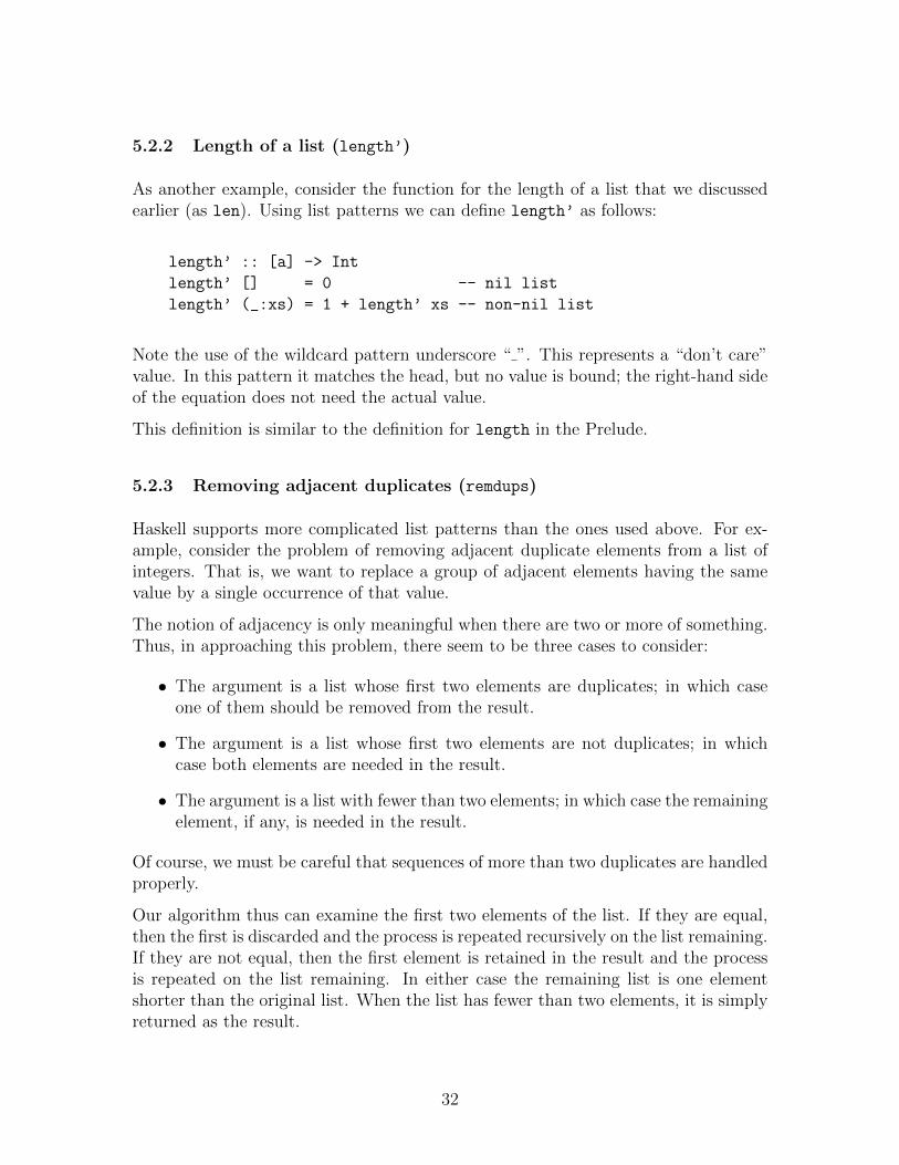
5.2.2 Length of a list (length’)

As another example, consider the function for the length of a list that we discussedearlier (as len). Using list patterns we can define length’ as follows:

length’ :: [a] -> Int

length’ [] = 0 -- nil list

length’ (_:xs) = 1 + length’ xs -- non-nil list

Note the use of the wildcard pattern underscore “ ”. This represents a “don’t care”value. In this pattern it matches the head, but no value is bound; the right-hand sideof the equation does not need the actual value.

This definition is similar to the definition for length in the Prelude.

5.2.3 Removing adjacent duplicates (remdups)

Haskell supports more complicated list patterns than the ones used above. For ex-ample, consider the problem of removing adjacent duplicate elements from a list ofintegers. That is, we want to replace a group of adjacent elements having the samevalue by a single occurrence of that value.

The notion of adjacency is only meaningful when there are two or more of something.Thus, in approaching this problem, there seem to be three cases to consider:

• The argument is a list whose first two elements are duplicates; in which caseone of them should be removed from the result.

• The argument is a list whose first two elements are not duplicates; in whichcase both elements are needed in the result.

• The argument is a list with fewer than two elements; in which case the remainingelement, if any, is needed in the result.

Of course, we must be careful that sequences of more than two duplicates are handledproperly.

Our algorithm thus can examine the first two elements of the list. If they are equal,then the first is discarded and the process is repeated recursively on the list remaining.If they are not equal, then the first element is retained in the result and the processis repeated on the list remaining. In either case the remaining list is one elementshorter than the original list. When the list has fewer than two elements, it is simplyreturned as the result.

32

In Haskell, we can define function remdups as follows:

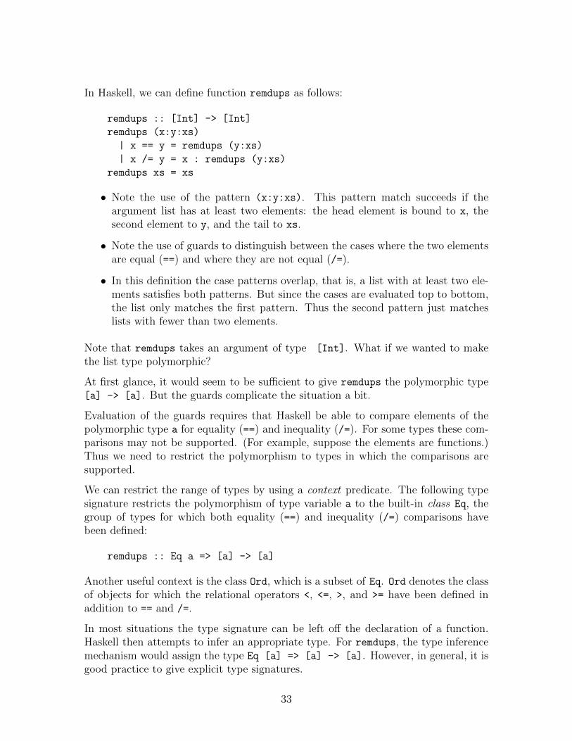
remdups :: [Int] -> [Int]

remdups (x:y:xs)

| x == y = remdups (y:xs)

| x /= y = x : remdups (y:xs)

remdups xs = xs

• Note the use of the pattern (x:y:xs). This pattern match succeeds if theargument list has at least two elements: the head element is bound to x, thesecond element to y, and the tail to xs.

• Note the use of guards to distinguish between the cases where the two elementsare equal (==) and where they are not equal (/=).

• In this definition the case patterns overlap, that is, a list with at least two ele-ments satisfies both patterns. But since the cases are evaluated top to bottom,the list only matches the first pattern. Thus the second pattern just matcheslists with fewer than two elements.

Note that remdups takes an argument of type [Int]. What if we wanted to makethe list type polymorphic?

At first glance, it would seem to be sufficient to give remdups the polymorphic type[a] -> [a]. But the guards complicate the situation a bit.

Evaluation of the guards requires that Haskell be able to compare elements of thepolymorphic type a for equality (==) and inequality (/=). For some types these com-parisons may not be supported. (For example, suppose the elements are functions.)Thus we need to restrict the polymorphism to types in which the comparisons aresupported.

We can restrict the range of types by using a context predicate. The following typesignature restricts the polymorphism of type variable a to the built-in class Eq, thegroup of types for which both equality (==) and inequality (/=) comparisons havebeen defined:

remdups :: Eq a => [a] -> [a]

Another useful context is the class Ord, which is a subset of Eq. Ord denotes the classof objects for which the relational operators <, <=, >, and >= have been defined inaddition to == and /=.

In most situations the type signature can be left off the declaration of a function.Haskell then attempts to infer an appropriate type. For remdups, the type inferencemechanism would assign the type Eq [a] => [a] -> [a]. However, in general, it isgood practice to give explicit type signatures.

33

5.2.4 More example patterns

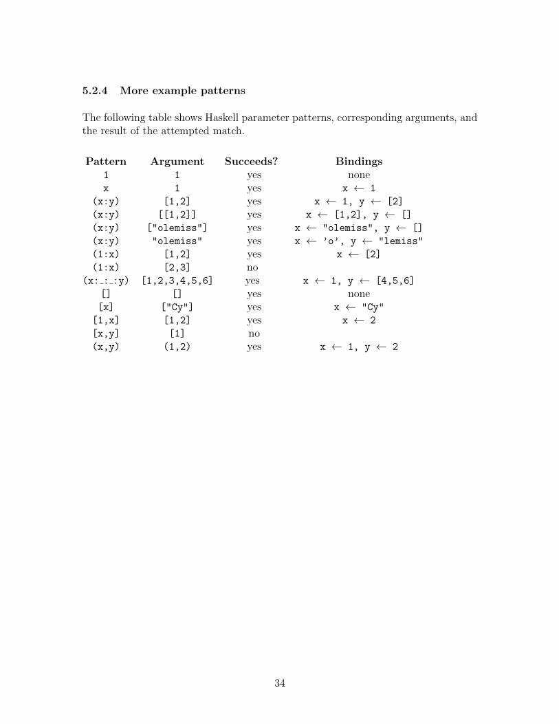
The following table shows Haskell parameter patterns, corresponding arguments, andthe result of the attempted match.

Pattern Argument Succeeds? Bindings1 1 yes nonex 1 yes x ← 1

(x:y) [1,2] yes x ← 1, y ← [2]

(x:y) [[1,2]] yes x ← [1,2], y ← []

(x:y) ["olemiss"] yes x ← "olemiss", y ← []

(x:y) "olemiss" yes x ← ’o’, y ← "lemiss"

(1:x) [1,2] yes x ← [2]

(1:x) [2,3] no(x: : :y) [1,2,3,4,5,6] yes x ← 1, y ← [4,5,6]

[] [] yes none[x] ["Cy"] yes x ← "Cy"

[1,x] [1,2] yes x ← 2

[x,y] [1] no(x,y) (1,2) yes x ← 1, y ← 2

34

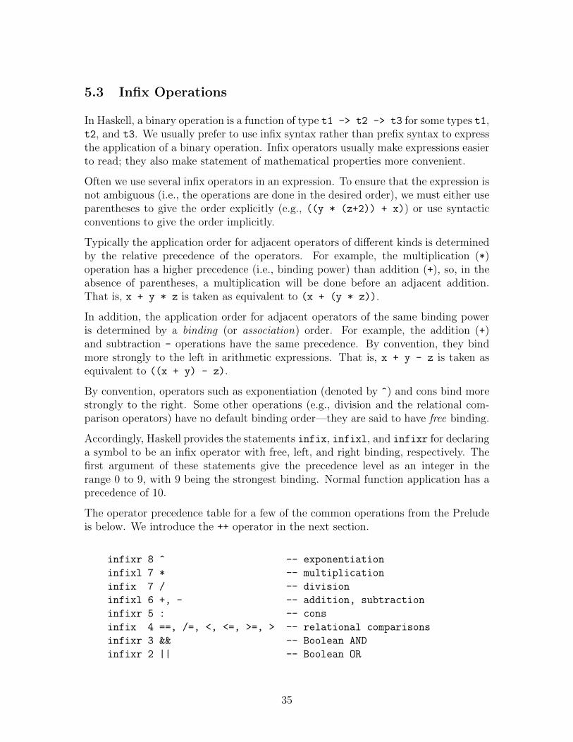
5.3 Infix Operations

In Haskell, a binary operation is a function of type t1 -> t2 -> t3 for some types t1,t2, and t3. We usually prefer to use infix syntax rather than prefix syntax to expressthe application of a binary operation. Infix operators usually make expressions easierto read; they also make statement of mathematical properties more convenient.

Often we use several infix operators in an expression. To ensure that the expression isnot ambiguous (i.e., the operations are done in the desired order), we must either useparentheses to give the order explicitly (e.g., ((y * (z+2)) + x)) or use syntacticconventions to give the order implicitly.

Typically the application order for adjacent operators of different kinds is determinedby the relative precedence of the operators. For example, the multiplication (*)operation has a higher precedence (i.e., binding power) than addition (+), so, in theabsence of parentheses, a multiplication will be done before an adjacent addition.That is, x + y * z is taken as equivalent to (x + (y * z)).

In addition, the application order for adjacent operators of the same binding poweris determined by a binding (or association) order. For example, the addition (+)and subtraction - operations have the same precedence. By convention, they bindmore strongly to the left in arithmetic expressions. That is, x + y - z is taken asequivalent to ((x + y) - z).

By convention, operators such as exponentiation (denoted by ^) and cons bind morestrongly to the right. Some other operations (e.g., division and the relational com-parison operators) have no default binding order—they are said to have free binding.

Accordingly, Haskell provides the statements infix, infixl, and infixr for declaringa symbol to be an infix operator with free, left, and right binding, respectively. Thefirst argument of these statements give the precedence level as an integer in therange 0 to 9, with 9 being the strongest binding. Normal function application has aprecedence of 10.

The operator precedence table for a few of the common operations from the Preludeis below. We introduce the ++ operator in the next section.

infixr 8 ^ -- exponentiation

infixl 7 * -- multiplication

infix 7 / -- division

infixl 6 +, - -- addition, subtraction

infixr 5 : -- cons

infix 4 ==, /=, <, <=, >=, > -- relational comparisons

infixr 3 && -- Boolean AND

infixr 2 || -- Boolean OR

35

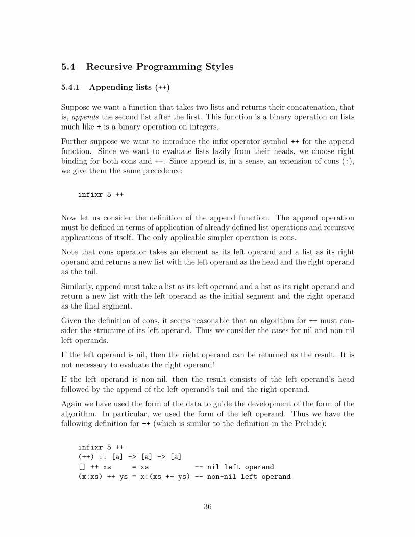
5.4 Recursive Programming Styles

5.4.1 Appending lists (++)

Suppose we want a function that takes two lists and returns their concatenation, thatis, appends the second list after the first. This function is a binary operation on listsmuch like + is a binary operation on integers.

Further suppose we want to introduce the infix operator symbol ++ for the appendfunction. Since we want to evaluate lists lazily from their heads, we choose rightbinding for both cons and ++. Since append is, in a sense, an extension of cons (:),we give them the same precedence:

infixr 5 ++

Now let us consider the definition of the append function. The append operationmust be defined in terms of application of already defined list operations and recursiveapplications of itself. The only applicable simpler operation is cons.

Note that cons operator takes an element as its left operand and a list as its rightoperand and returns a new list with the left operand as the head and the right operandas the tail.

Similarly, append must take a list as its left operand and a list as its right operand andreturn a new list with the left operand as the initial segment and the right operandas the final segment.

Given the definition of cons, it seems reasonable that an algorithm for ++ must con-sider the structure of its left operand. Thus we consider the cases for nil and non-nilleft operands.

If the left operand is nil, then the right operand can be returned as the result. It isnot necessary to evaluate the right operand!

If the left operand is non-nil, then the result consists of the left operand’s headfollowed by the append of the left operand’s tail and the right operand.

Again we have used the form of the data to guide the development of the form of thealgorithm. In particular, we used the form of the left operand. Thus we have thefollowing definition for ++ (which is similar to the definition in the Prelude):

infixr 5 ++

(++) :: [a] -> [a] -> [a]

[] ++ xs = xs -- nil left operand

(x:xs) ++ ys = x:(xs ++ ys) -- non-nil left operand

36

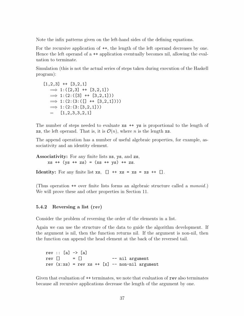
Note the infix patterns given on the left-hand sides of the defining equations.

For the recursive application of ++, the length of the left operand decreases by one.Hence the left operand of a ++ application eventually becomes nil, allowing the eval-uation to terminate.

Simulation (this is not the actual series of steps taken during execution of the Haskellprogram):

[1,2,3] ++ [3,2,1]

=⇒ 1:([2,3] ++ [3,2,1])

=⇒ 1:(2:([3] ++ [3,2,1]))

=⇒ 1:(2:(3:([] ++ [3,2,1])))

=⇒ 1:(2:(3:[3,2,1]))

= [1,2,3,3,2,1]

The number of steps needed to evaluate xs ++ ys is proportional to the length ofxs, the left operand. That is, it is O(n), where n is the length xs.

The append operation has a number of useful algebraic properties, for example, as-sociativity and an identity element.

Associativity: For any finite lists xs, ys, and zs,xs ++ (ys ++ zs) = (xs ++ ys) ++ zs.

Identity: For any finite list xs, [] ++ xs = xs = xs ++ [].

(Thus operation ++ over finite lists forms an algebraic structure called a monoid .)We will prove these and other properties in Section 11.

5.4.2 Reversing a list (rev)

Consider the problem of reversing the order of the elements in a list.

Again we can use the structure of the data to guide the algorithm development. Ifthe argument is nil, then the function returns nil. If the argument is non-nil, thenthe function can append the head element at the back of the reversed tail.

rev :: [a] -> [a]

rev [] = [] -- nil argument

rev (x:xs) = rev xs ++ [x] -- non-nil argument

Given that evaluation of ++ terminates, we note that evaluation of rev also terminatesbecause all recursive applications decrease the length of the argument by one.

37

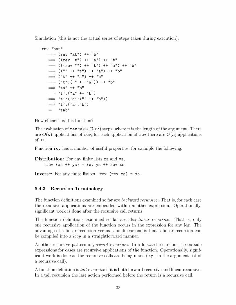
Simulation (this is not the actual series of steps taken during execution):

rev "bat"

=⇒ (rev "at") ++ "b"

=⇒ ((rev "t") ++ "a") ++ "b"

=⇒ (((rev "") ++ "t") ++ "a") ++ "b"

=⇒ (("" ++ "t") ++ "a") ++ "b"

=⇒ ("t" ++ "a") ++ "b"

=⇒ (’t’:("" ++ "a")) ++ "b"

=⇒ "ta" ++ "b"

=⇒ ’t’:("a" ++ "b")

=⇒ ’t’:(’a’:("" ++ "b"))

=⇒ ’t’:(’a’:"b")

= "tab"

How efficient is this function?

The evaluation of rev takesO(n2) steps, where n is the length of the argument. Thereare O(n) applications of rev; for each application of rev there are O(n) applicationsof ++.

Function rev has a number of useful properties, for example the following:

Distribution: For any finite lists xs and ys,rev (xs ++ ys) = rev ys ++ rev xs.

Inverse: For any finite list xs, rev (rev xs) = xs.

5.4.3 Recursion Terminology

The function definitions examined so far are backward recursive. That is, for each casethe recursive applications are embedded within another expression. Operationally,significant work is done after the recursive call returns.

The function definitions examined so far are also linear recursive. That is, onlyone recursive application of the function occurs in the expression for any leg. Theadvantage of a linear recursion versus a nonlinear one is that a linear recursion canbe compiled into a loop in a straightforward manner.

Another recursive pattern is forward recursion. In a forward recursion, the outsideexpressions for cases are recursive applications of the function. Operationally, signif-icant work is done as the recursive calls are being made (e.g., in the argument list ofa recursive call).

A function definition is tail recursive if it is both forward recursive and linear recursive.In a tail recursion the last action performed before the return is a recursive call.

38

Tail recursive definitions are easy to compile into efficient loops. There is no need tosave the state of the unevaluated expressions for the higher level calls; the result ofa recursive call can be returned directly as the caller’s result. This process is calledtail call optimization, tail call elimination), or sometimes proper tail calls.

5.4.4 Tail recursive reverse (reverse’)

Now let’s look at the problem of reversing a list again to see whether we can devisea “more efficient” tail recursive solution.

The common technique for converting a backward linear recursive definition like rev

into a tail recursive definition is to use an accumulating parameter (also called an ac-cumulator) to build up the desired result incrementally. A possible definition follows:

rev’ [] ys = ys

rev’ (x:xs) ys = rev’ xs (x:ys)

In this definition parameter ys is the accumulating parameter. The head of the firstargument becomes the new head of the accumulating parameter for the tail recursivecall. The tail of the first argument becomes the new first argument for the tailrecursive call.

We know that rev’ terminates because, for each recursive application, the length ofthe first argument decreases toward the base case of [].

We note that rev xs is equivalent to rev’ xs []. We will prove this in Section 11.6.

To define a single-argument replacement for rev, we can embed the definition of rev’as an auxiliary function within the definition of a new function reverse’. (This issimilar to function reverse in the Prelude.)

reverse’ :: [a] -> [a]

reverse’ xs = rev xs []

where rev [] ys = ys

rev (x:xs) ys = rev xs (x:ys)

The where clause introduces the local definition rev’ that is only known within theright-hand side of the defining equation for the function reverse’.

How efficient is this function?

The evaluation of reverse’ takes O(n) steps, where n is the length of the argu-ment. There is one application of rev’ for each element; rev’ requires a single consoperation in the accumulating parameter.

39

Where did the increase in efficiency come from? Each application of rev applies ++,a linear time (i.e., O(n) ) function. In rev’, we replaced the applications of ++ byapplications of cons, a constant time (i.e., O(1) ) function.

In addition, a compiler or interpreter that does tail call optimization can translatethis tail recursive call into a loop on the host machine.

5.4.5 Local definitions (let and where)

The let expression is useful whenever a nested set of definitions is required. It hasthe following syntax:

let local definitions in expression

A let may be used anywhere that an expression my appear in a Haskell program.

For example, consider a function f that takes a list of integers and returns a list oftheir squares incremented by one:

f :: [Int] -> [Int]

f [] = []

f xs = let square a = a * a

one = 1

(y:ys) = xs

in (square y + one) : f ys

• square represents a function of one variable.

• one represents a constant, that is, a function of zero variables.

• (y:ys) represents a pattern match binding against argument xs of f.

• Reference to y or ys when argument xs of f is nil results in an error.

• Local definitions square, one, y, and ys all come into scope simultaneously;their scope is the expression following the in keyword.

• Local definitions may access identifiers in outer scopes (e.g., xs in definition of(y:ys)) and have definitions nested within themselves.

• Local definitions may be recursive and call each other.

The let clause introduces symbols in a bottom-up manner: it introduces symbolsbefore they are used.

40

The where clause is similar semantically, but it introduces symbols in a top-downmanner: the symbols are used and then defined in a where that follows.

The where clause is more versatile than the let. It allows the scope of local definitionsto span over several guarded equations while a let’s scope is restricted to the right-hand side of one equation.

For example, consider the definition:

g :: Int -> Int

g n | (n ‘mod‘ 3) == x = x

| (n ‘mod‘ 3) == y = y

| (n ‘mod‘ 3) == z = z

where x = 0

y = 1

z = 2

• The scope of this where clause is over all three guards and their respective right-hand sides. (Note that the where begins in the same column as the = ratherthan to the right as in rev’.)

• Note the use of the modulo function mod as an infix operator. The backquotes(‘) around a function name denotes the infix use of the function.

5.4.6 Fibonacci numbers

The first two elements of the (second-order) Fibonacci sequence are 0 and 1; eachsuccessive element is the sum of the previous two elements. Element n of this sequencecan be computed by the following Haskell function:

fib :: Int -> Int

fib 0 = 0

fib 1 = 1

fib n | n > 1 = fib (n-2) + fib (n-1)

This function definition uses the n > 1 guard on the third pattern to match naturalnumbers at least 2.

An equivalent, but more efficient, definition uses forward recursion with two additionalparameters to avoid recomputing Fibonacci numbers:

fib’ :: Int -> Int

fib’ n = fib’’ n 0 1

where fib’’ 0 p q = p

fib’’ n p q | n > 0 = fib’’ (n-1) q (p+q)

41

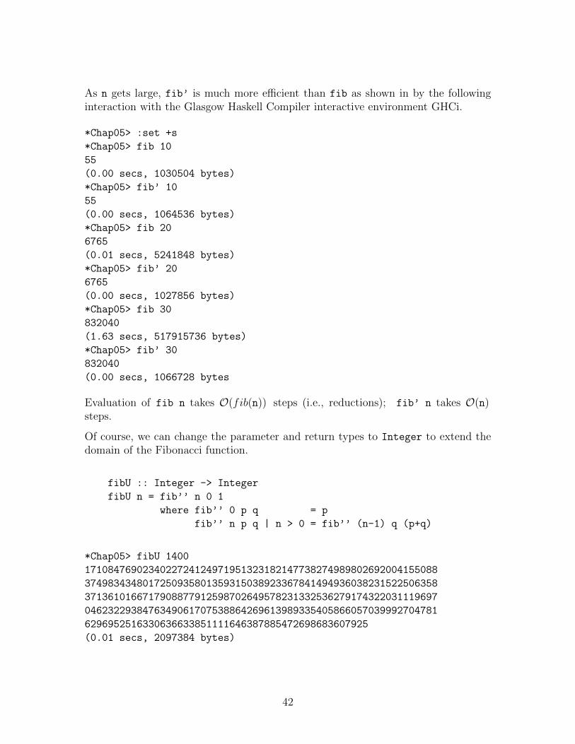
As n gets large, fib’ is much more efficient than fib as shown in by the followinginteraction with the Glasgow Haskell Compiler interactive environment GHCi.

*Chap05> :set +s

*Chap05> fib 10

55

(0.00 secs, 1030504 bytes)

*Chap05> fib’ 10

55

(0.00 secs, 1064536 bytes)

*Chap05> fib 20

6765

(0.01 secs, 5241848 bytes)

*Chap05> fib’ 20

6765

(0.00 secs, 1027856 bytes)

*Chap05> fib 30

832040

(1.63 secs, 517915736 bytes)

*Chap05> fib’ 30

832040

(0.00 secs, 1066728 bytes

Evaluation of fib n takes O(fib(n)) steps (i.e., reductions); fib’ n takes O(n)steps.

Of course, we can change the parameter and return types to Integer to extend thedomain of the Fibonacci function.

fibU :: Integer -> Integer

fibU n = fib’’ n 0 1

where fib’’ 0 p q = p

fib’’ n p q | n > 0 = fib’’ (n-1) q (p+q)

*Chap05> fibU 1400

1710847690234022724124971951323182147738274989802692004155088

3749834348017250935801359315038923367841494936038231522506358

3713610166717908877912598702649578231332536279174322031119697

0462322938476349061707538864269613989335405866057039992704781

6296952516330636633851111646387885472698683607925

(0.01 secs, 2097384 bytes)

42

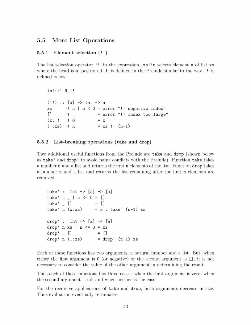
5.5 More List Operations

5.5.1 Element selection (!!)

The list selection operator !! in the expression xs!!n selects element n of list xs

where the head is in position 0. It is defined in the Prelude similar to the way !! isdefined below:

infixl 9 !!

(!!) :: [a] -> Int -> a

xs !! n | n < 0 = error "!! negative index"

[] !! _ = error "!! index too large"

(x:_) !! 0 = x

(_:xs) !! n = xs !! (n-1)

5.5.2 List-breaking operations (take and drop)

Two additional useful functions from the Prelude are take and drop (shown belowas take’ and drop’ to avoid name conflicts with the Prelude). Function take takesa number n and a list and returns the first n elements of the list. Function drop takesa number n and a list and returns the list remaining after the first n elements areremoved.

take’ :: Int -> [a] -> [a]

take’ n _ | n <= 0 = []

take’ _ [] = []

take’ n (x:xs) = x : take’ (n-1) xs

drop’ :: Int -> [a] -> [a]

drop’ n xs | n <= 0 = xs

drop’ _ [] = []

drop’ n (_:xs) = drop’ (n-1) xs

Each of these functions has two arguments, a natural number and a list. But, wheneither the first argument is 0 (or negative) or the second argument is [], it is notnecessary to consider the value of the other argument in determining the result.

Thus each of these functions has three cases: when the first argument is zero, whenthe second argument is nil, and when neither is the case.

For the recursive applications of take and drop, both arguments decrease in size.Thus evaluation eventually terminates.

43

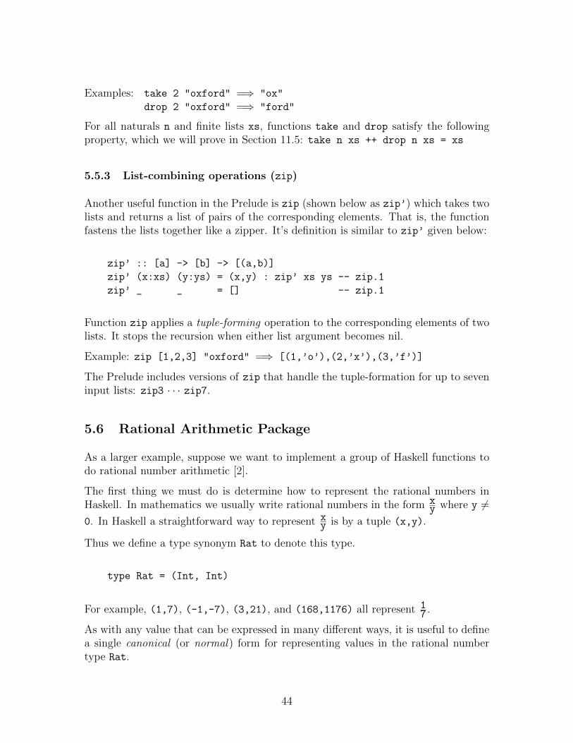
Examples: take 2 "oxford" =⇒ "ox"

drop 2 "oxford" =⇒ "ford"

For all naturals n and finite lists xs, functions take and drop satisfy the followingproperty, which we will prove in Section 11.5: take n xs ++ drop n xs = xs

5.5.3 List-combining operations (zip)

Another useful function in the Prelude is zip (shown below as zip’) which takes twolists and returns a list of pairs of the corresponding elements. That is, the functionfastens the lists together like a zipper. It’s definition is similar to zip’ given below:

zip’ :: [a] -> [b] -> [(a,b)]

zip’ (x:xs) (y:ys) = (x,y) : zip’ xs ys -- zip.1

zip’ _ _ = [] -- zip.1

Function zip applies a tuple-forming operation to the corresponding elements of twolists. It stops the recursion when either list argument becomes nil.

Example: zip [1,2,3] "oxford" =⇒ [(1,’o’),(2,’x’),(3,’f’)]

The Prelude includes versions of zip that handle the tuple-formation for up to seveninput lists: zip3 · · · zip7.

5.6 Rational Arithmetic Package

As a larger example, suppose we want to implement a group of Haskell functions todo rational number arithmetic [2].

The first thing we must do is determine how to represent the rational numbers inHaskell. In mathematics we usually write rational numbers in the form x

y where y 6=0. In Haskell a straightforward way to represent x

y is by a tuple (x,y).

Thus we define a type synonym Rat to denote this type.

type Rat = (Int, Int)

For example, (1,7), (-1,-7), (3,21), and (168,1176) all represent 17 .

As with any value that can be expressed in many different ways, it is useful to definea single canonical (or normal) form for representing values in the rational numbertype Rat.

44

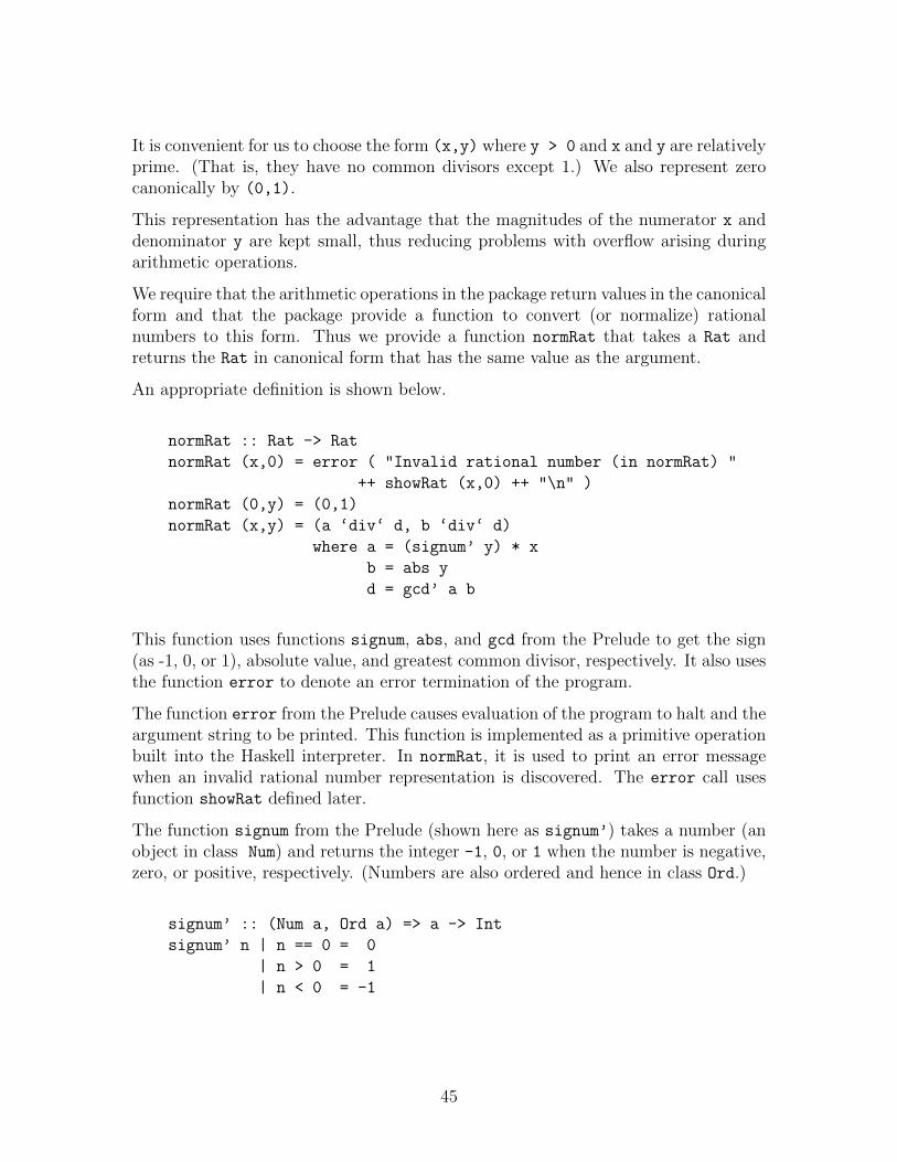
It is convenient for us to choose the form (x,y) where y > 0 and x and y are relativelyprime. (That is, they have no common divisors except 1.) We also represent zerocanonically by (0,1).

This representation has the advantage that the magnitudes of the numerator x anddenominator y are kept small, thus reducing problems with overflow arising duringarithmetic operations.

We require that the arithmetic operations in the package return values in the canonicalform and that the package provide a function to convert (or normalize) rationalnumbers to this form. Thus we provide a function normRat that takes a Rat andreturns the Rat in canonical form that has the same value as the argument.

An appropriate definition is shown below.

normRat :: Rat -> Rat

normRat (x,0) = error ( "Invalid rational number (in normRat) "

++ showRat (x,0) ++ "\n" )

normRat (0,y) = (0,1)

normRat (x,y) = (a ‘div‘ d, b ‘div‘ d)

where a = (signum’ y) * x

b = abs y

d = gcd’ a b

This function uses functions signum, abs, and gcd from the Prelude to get the sign(as -1, 0, or 1), absolute value, and greatest common divisor, respectively. It also usesthe function error to denote an error termination of the program.

The function error from the Prelude causes evaluation of the program to halt and theargument string to be printed. This function is implemented as a primitive operationbuilt into the Haskell interpreter. In normRat, it is used to print an error messagewhen an invalid rational number representation is discovered. The error call usesfunction showRat defined later.

The function signum from the Prelude (shown here as signum’) takes a number (anobject in class Num) and returns the integer -1, 0, or 1 when the number is negative,zero, or positive, respectively. (Numbers are also ordered and hence in class Ord.)

signum’ :: (Num a, Ord a) => a -> Int

signum’ n | n == 0 = 0

| n > 0 = 1

| n < 0 = -1

45

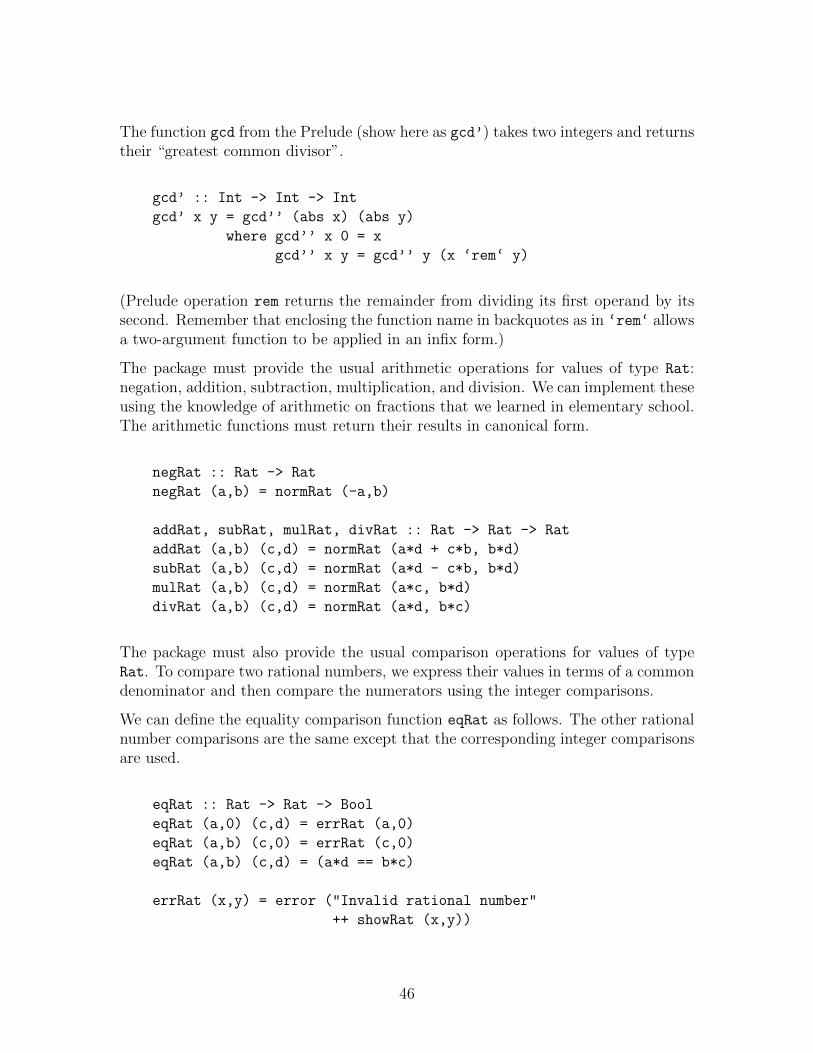
The function gcd from the Prelude (show here as gcd’) takes two integers and returnstheir “greatest common divisor”.

gcd’ :: Int -> Int -> Int

gcd’ x y = gcd’’ (abs x) (abs y)

where gcd’’ x 0 = x

gcd’’ x y = gcd’’ y (x ‘rem‘ y)

(Prelude operation rem returns the remainder from dividing its first operand by itssecond. Remember that enclosing the function name in backquotes as in ‘rem‘ allowsa two-argument function to be applied in an infix form.)

The package must provide the usual arithmetic operations for values of type Rat:negation, addition, subtraction, multiplication, and division. We can implement theseusing the knowledge of arithmetic on fractions that we learned in elementary school.The arithmetic functions must return their results in canonical form.

negRat :: Rat -> Rat

negRat (a,b) = normRat (-a,b)

addRat, subRat, mulRat, divRat :: Rat -> Rat -> Rat

addRat (a,b) (c,d) = normRat (a*d + c*b, b*d)

subRat (a,b) (c,d) = normRat (a*d - c*b, b*d)

mulRat (a,b) (c,d) = normRat (a*c, b*d)

divRat (a,b) (c,d) = normRat (a*d, b*c)

The package must also provide the usual comparison operations for values of typeRat. To compare two rational numbers, we express their values in terms of a commondenominator and then compare the numerators using the integer comparisons.

We can define the equality comparison function eqRat as follows. The other rationalnumber comparisons are the same except that the corresponding integer comparisonsare used.

eqRat :: Rat -> Rat -> Bool

eqRat (a,0) (c,d) = errRat (a,0)

eqRat (a,b) (c,0) = errRat (c,0)

eqRat (a,b) (c,d) = (a*d == b*c)

errRat (x,y) = error ("Invalid rational number"

++ showRat (x,y))

46

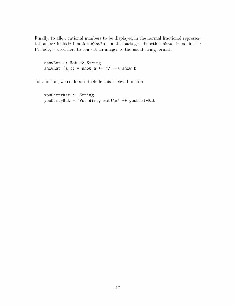
Finally, to allow rational numbers to be displayed in the normal fractional represen-tation, we include function showRat in the package. Function show, found in thePrelude, is used here to convert an integer to the usual string format.

showRat :: Rat -> String

showRat (a,b) = show a ++ "/" ++ show b

Just for fun, we could also include this useless function:

youDirtyRat :: String

youDirtyRat = "You dirty rat!\n" ++ youDirtyRat

47

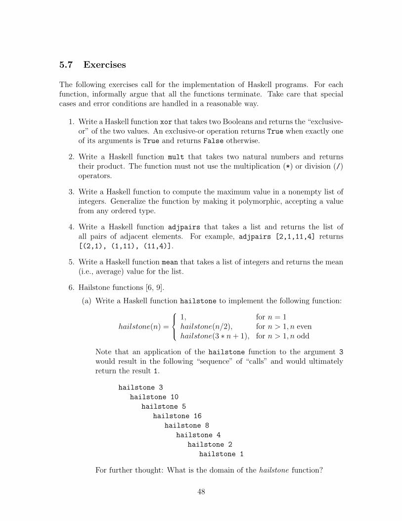
5.7 Exercises

The following exercises call for the implementation of Haskell programs. For eachfunction, informally argue that all the functions terminate. Take care that specialcases and error conditions are handled in a reasonable way.

1. Write a Haskell function xor that takes two Booleans and returns the “exclusive-or” of the two values. An exclusive-or operation returns True when exactly oneof its arguments is True and returns False otherwise.

2. Write a Haskell function mult that takes two natural numbers and returnstheir product. The function must not use the multiplication (*) or division (/)operators.

3. Write a Haskell function to compute the maximum value in a nonempty list ofintegers. Generalize the function by making it polymorphic, accepting a valuefrom any ordered type.

4. Write a Haskell function adjpairs that takes a list and returns the list ofall pairs of adjacent elements. For example, adjpairs [2,1,11,4] returns[(2,1), (1,11), (11,4)].

5. Write a Haskell function mean that takes a list of integers and returns the mean(i.e., average) value for the list.

6. Hailstone functions [6, 9].

(a) Write a Haskell function hailstone to implement the following function:

hailstone(n) =

1, for n = 1hailstone(n/2), for n > 1, n evenhailstone(3 ∗ n+ 1), for n > 1, n odd

Note that an application of the hailstone function to the argument 3

would result in the following “sequence” of “calls” and would ultimatelyreturn the result 1.

hailstone 3

hailstone 10

hailstone 5

hailstone 16

hailstone 8

hailstone 4

hailstone 2

hailstone 1

For further thought: What is the domain of the hailstone function?

48

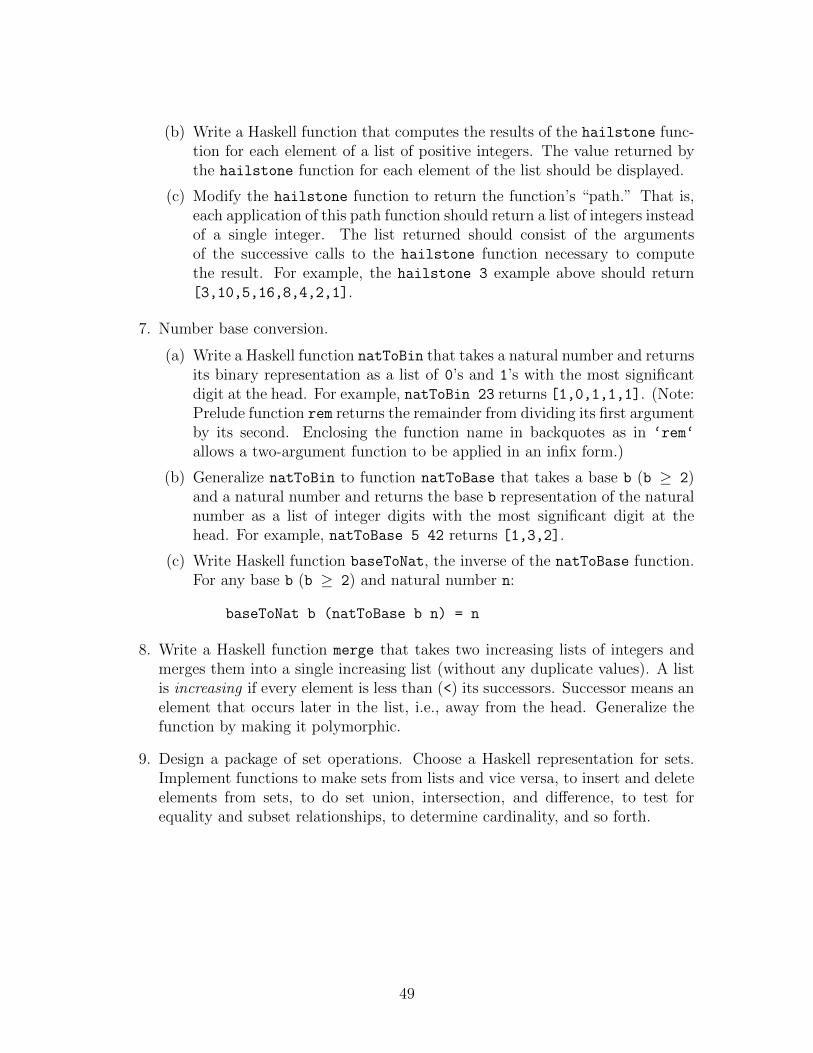
(b) Write a Haskell function that computes the results of the hailstone func-tion for each element of a list of positive integers. The value returned bythe hailstone function for each element of the list should be displayed.

(c) Modify the hailstone function to return the function’s “path.” That is,each application of this path function should return a list of integers insteadof a single integer. The list returned should consist of the argumentsof the successive calls to the hailstone function necessary to computethe result. For example, the hailstone 3 example above should return[3,10,5,16,8,4,2,1].

7. Number base conversion.

(a) Write a Haskell function natToBin that takes a natural number and returnsits binary representation as a list of 0’s and 1’s with the most significantdigit at the head. For example, natToBin 23 returns [1,0,1,1,1]. (Note:Prelude function rem returns the remainder from dividing its first argumentby its second. Enclosing the function name in backquotes as in ‘rem‘

allows a two-argument function to be applied in an infix form.)

(b) Generalize natToBin to function natToBase that takes a base b (b ≥ 2)and a natural number and returns the base b representation of the naturalnumber as a list of integer digits with the most significant digit at thehead. For example, natToBase 5 42 returns [1,3,2].

(c) Write Haskell function baseToNat, the inverse of the natToBase function.For any base b (b ≥ 2) and natural number n:

baseToNat b (natToBase b n) = n

8. Write a Haskell function merge that takes two increasing lists of integers andmerges them into a single increasing list (without any duplicate values). A listis increasing if every element is less than (<) its successors. Successor means anelement that occurs later in the list, i.e., away from the head. Generalize thefunction by making it polymorphic.

9. Design a package of set operations. Choose a Haskell representation for sets.Implement functions to make sets from lists and vice versa, to insert and deleteelements from sets, to do set union, intersection, and difference, to test forequality and subset relationships, to determine cardinality, and so forth.

49

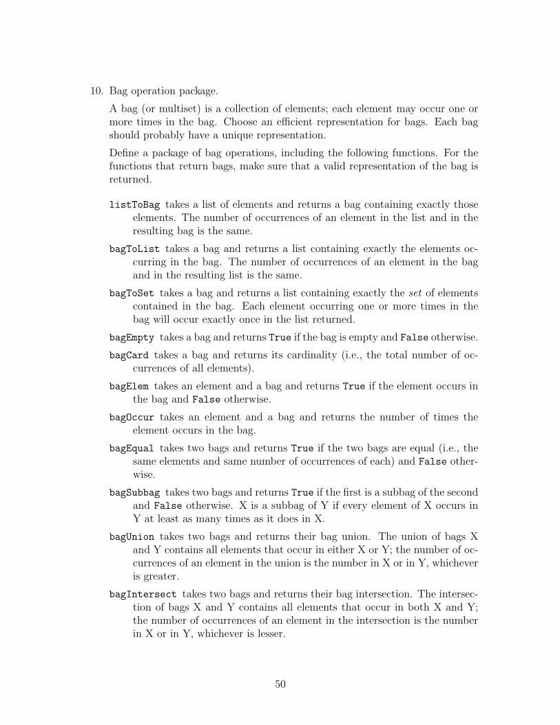
10. Bag operation package.

A bag (or multiset) is a collection of elements; each element may occur one ormore times in the bag. Choose an efficient representation for bags. Each bagshould probably have a unique representation.

Define a package of bag operations, including the following functions. For thefunctions that return bags, make sure that a valid representation of the bag isreturned.

listToBag takes a list of elements and returns a bag containing exactly thoseelements. The number of occurrences of an element in the list and in theresulting bag is the same.

bagToList takes a bag and returns a list containing exactly the elements oc-curring in the bag. The number of occurrences of an element in the bagand in the resulting list is the same.

bagToSet takes a bag and returns a list containing exactly the set of elementscontained in the bag. Each element occurring one or more times in thebag will occur exactly once in the list returned.

bagEmpty takes a bag and returns True if the bag is empty and False otherwise.

bagCard takes a bag and returns its cardinality (i.e., the total number of oc-currences of all elements).

bagElem takes an element and a bag and returns True if the element occurs inthe bag and False otherwise.

bagOccur takes an element and a bag and returns the number of times theelement occurs in the bag.

bagEqual takes two bags and returns True if the two bags are equal (i.e., thesame elements and same number of occurrences of each) and False other-wise.

bagSubbag takes two bags and returns True if the first is a subbag of the secondand False otherwise. X is a subbag of Y if every element of X occurs inY at least as many times as it does in X.

bagUnion takes two bags and returns their bag union. The union of bags Xand Y contains all elements that occur in either X or Y; the number of oc-currences of an element in the union is the number in X or in Y, whicheveris greater.

bagIntersect takes two bags and returns their bag intersection. The intersec-tion of bags X and Y contains all elements that occur in both X and Y;the number of occurrences of an element in the intersection is the numberin X or in Y, whichever is lesser.

50

bagSum takes two bags and returns their bag sum. The sum of bags X and Ycontains all elements that occur in X or Y; the number of occurrences ofan element is the sum of the number of occurrences in X and Y.

bagDiff takes two bags and returns the bag difference, first argument minusthe second. The difference of bags X and Y contains all elements of X thatoccur in Y fewer times; the number of occurrences of an element in thedifference is the number of occurrences in X minus the number in Y.

bagInsert takes an element and a bag and returns the bag with the elementinserted. Bag insertion either adds a single occurrence of a new elementto the bag or increases the number of occurrences of an existing elementby one.

bagDelete takes an element and a bag and returns the bag with the elementdeleted. Bag deletion either removes a single occurrence of the elementfrom the bag or decreases the number of occurrences of the element byone.

11. Unbounded precision arithmetic package for natural numbers (i.e., nonnegativeintegers).

(a) Define a type synonym BigNat to represent these unbounded precisionnatural numbers as lists of Int. Let each element of the list denote adecimal digit of the “big natural” number represented, with the least sig-nificant digit at the head of the list and the remaining digits given in orderof increasing significance. For example, the integer value 22345678901 isrepresented as [1,0,9,8,7,6,5,4,3,2,2]. Use the following “canonical”representation: the value 0 is represented by the list [0] and positivenumbers by a list without “leading” 0 digits (i.e., 126 is [6,2,1] not[6,2,1,0,0]). You may use the nil list [ ] to denote an error value.

Define a package of basic arithmetic operations, including the followingfunctions. Make sure that BigNat values returned by these functions arein canonical form.

intToBig takes a nonnegative Int and returns the BigNat with the samevalue.

strToBig takes a String containing the value of the number in the “usual”format (i.e., decimal digits, left to right in order of decreasing signifi-cance with zero or more leading spaces, but with no spaces or punctu-ation embedded within the number) and returns the BigNat with thesame value.

bigToStr takes a BigNat and returns a String containing the value of thenumber in the “usual” format (i.e., left to right in order of decreasingsignificance with no spaces or punctuation).

51

bigComp takes two BigNats and returns the Int value -1 if the value ofthe first is less than the value of the second, the value 0 if they areequal, and the value 1 if the first is greater than the second.

bigAdd takes two BigNats and returns their sum as a BigNat.

bigSub takes two BigNats and returns their difference as a BigNat, firstargument minus the second.

bigMult takes two BigNats and returns their product as a BigNat.

(b) Use the package to generate a table of factorials for the naturals 0 through25. Print the values from the table in two right-justified columns, with thenumber on the left and its factorial on the right. (Allow about 30 columnsfor 25!.)

(c) Use the package to generate a table of Fibonacci numbers for the naturals0 through 50.

(d) Generalize the package to handle signed integers. Add the following newfunction:

bigNeg returns the negation of its BigNat argument.

(e) Add the following functions to the package:

bigDiv takes two BigNats and returns, as a BigNat, the quotient fromdividing the first argument by the second.

bigRem takes two BigNats and returns, as a BigNat, the remainder fromdividing the first argument by the second.

12. Define the following set of text-justification functions. You may want to usePrelude functions like take, drop, and length.

spaces’ n returns a string of length n containing only space characters (i.e.,the character ’ ’).

left’ n xs returns a string of length n in which the string xs begins at thehead (i.e., left end). Examples: left’ 3 "ab" yields "ab "; left’ 3

"abcd" yields "abc".

right’ n xs returns a string of length n in which the string xs ends at thetail (i.e., right end). Examples: right’ 3 "bc" yields " bc"; right’ 3

"abcd" yields "bcd".

center’ n xs returns a string of length n in which the string xs is approxi-mately centered. Example: center’ 4 "bc" yields " bc ".

52

13. Consider simple mathematical expressions consisting of integer constants, vari-able names, parentheses, and the binary operators +, -, *, and /. For thepurposes of this exercise, an expression is a string that satisfies the following(extended) BNF grammar and lexical conventions :

expression ::= term { addOp term }term ::= factor { mulOp factor }factor ::= number

| identifier| ( expression )

• The characters in an input string are examined left to right to form “lex-ical tokens”. The tokens of the expression “language” consist of addOps,mulOps, identifiers, numbers, and left and right parentheses.

• An expression may contain space characters at any position except withina lexical token.

• An addOp token is either a “+” or a “-”; a mulOp token is either a “*” ora “/”.

• An identifier is a string of one or more contiguous characters such thatthe leftmost character is a letter and the remaining characters are ei-ther letters, digits, or underscore characters. Examples: “Hi1”, “lo23 1”,“this is 2 long ”

• A number is a string of one or more contiguous characters such that all(including the leftmost) are digits. Examples: “1”, “23456711”

• All identifier and number tokens extend as far to the right as possible. Forexample, consider the string “ A123 12B3+2 ) ”. (Note the space andright parenthesis characters). This string consists of the six tokens “A123”,“12”, “B3”, “+”, “2”, and “)”.

Define a Haskell function valid that takes a String and returns True if thestring is an expression as described above and returns False otherwise.

Hint: If you need to return more than one value from a function, you can do soby returning a tuple of those values. This tuple can be decomposed by Preludefunctions such as fst and snd.

Hint: Use of the where or let features can simplify many functions. Youmay find Prelude functions such as span, isSpace, isDigit, isAlpha, andisAlphanum useful.

Hint: You may want to consider organizing your program as a simple recursivedescent recognizer for the expression language.

53

14. Extend the mathematical expression recognizer of the previous exercise to eval-uate integer expressions with the given syntax. The four binary operations havetheir usual meanings.

Define a function eval e st that evaluates expression e using symbol tablest. If the expression e is syntactically valid, eval returns a pair (True,val)

where val is the value of e. If e is not valid, eval returns (False,0).

The symbol table consists of a list of pairs, in which the first component of apair is the variable name (a string) and the second is the variable’s value (aninteger).

Example: eval "(2+x) * y" [("y",3),("a",10),("x",8)] yields (True,30).

54

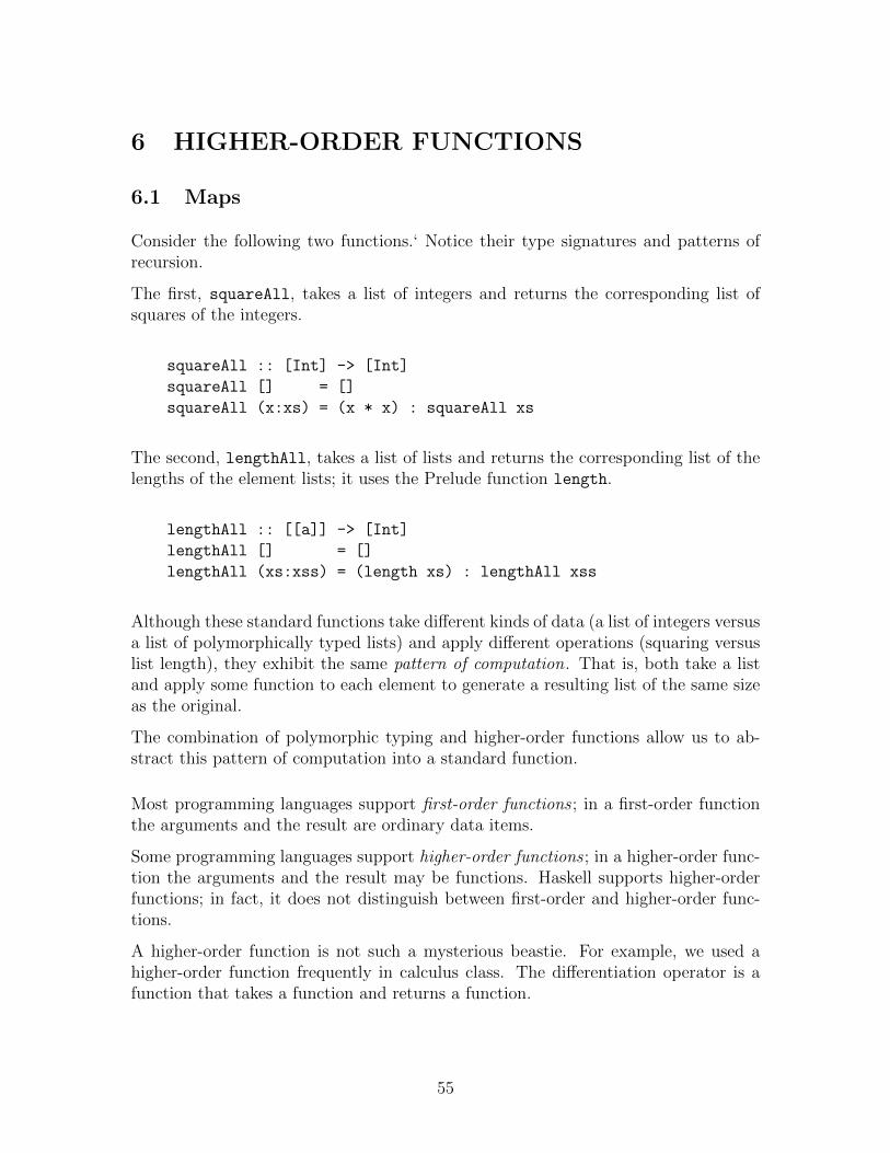
6 HIGHER-ORDER FUNCTIONS

6.1 Maps

Consider the following two functions.‘ Notice their type signatures and patterns ofrecursion.

The first, squareAll, takes a list of integers and returns the corresponding list ofsquares of the integers.

squareAll :: [Int] -> [Int]

squareAll [] = []

squareAll (x:xs) = (x * x) : squareAll xs

The second, lengthAll, takes a list of lists and returns the corresponding list of thelengths of the element lists; it uses the Prelude function length.

lengthAll :: [[a]] -> [Int]

lengthAll [] = []

lengthAll (xs:xss) = (length xs) : lengthAll xss

Although these standard functions take different kinds of data (a list of integers versusa list of polymorphically typed lists) and apply different operations (squaring versuslist length), they exhibit the same pattern of computation. That is, both take a listand apply some function to each element to generate a resulting list of the same sizeas the original.

The combination of polymorphic typing and higher-order functions allow us to ab-stract this pattern of computation into a standard function.

Most programming languages support first-order functions ; in a first-order functionthe arguments and the result are ordinary data items.

Some programming languages support higher-order functions ; in a higher-order func-tion the arguments and the result may be functions. Haskell supports higher-orderfunctions; in fact, it does not distinguish between first-order and higher-order func-tions.

A higher-order function is not such a mysterious beastie. For example, we used ahigher-order function frequently in calculus class. The differentiation operator is afunction that takes a function and returns a function.

55

Haskell abstracts the pattern of computation common to squareAll and lengthAll

as the very useful function map found in the Prelude (shown as map’ below to avoida name conflict):

map’ :: (a -> b) -> [a] -> [b] -- map

map’ f [] = []

map’ f (x:xs) = f x : map’ f xs

Function map takes a function f of type a -> b and a list of type [a], applies thefunction to each element of the list, and produces a list of type [b].

Thus we can redefine squareAll and lengthAll as follows:

squareAll2 :: [Int] -> [Int]

squareAll2 xs = map’ sq xs

where sq x = x * x

lengthAll2 :: [[a]] -> [Int]

lengthAll2 xss = map’ length xss

Above we defined Prelude function map as a recursive function that transforms theelements of a list one by one. However, it is often more useful to think of map in oneof two ways:

1. as a powerful list operator that transforms every element of the list. We cancombine map with other powerful operators to quickly construct powerful listprocessing programs.

We can consider map as operating on every element of the list simultaneously.In fact, an implementation could use separate processors to transform eachelement: this is essentially the map operation in Google’s mapReduce distributed“big data” processing framework.

2. as a operator node in a dataflow network. A stream of data objects flows intothe map node. The map node transforms each object by applying the argumentfunction. Then the data flows out to the next node of the network. The lazyevaluation of the Haskell functions enables such an implementation.

56

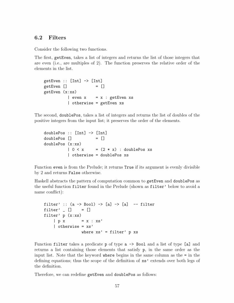
6.2 Filters

Consider the following two functions.

The first, getEven, takes a list of integers and returns the list of those integers thatare even (i.e., are multiples of 2). The function preserves the relative order of theelements in the list.

getEven :: [Int] -> [Int]

getEven [] = []

getEven (x:xs)

| even x = x : getEven xs

| otherwise = getEven xs

The second, doublePos, takes a list of integers and returns the list of doubles of thepositive integers from the input list; it preserves the order of the elements.

doublePos :: [Int] -> [Int]

doublePos [] = []

doublePos (x:xs)

| 0 < x = (2 * x) : doublePos xs

| otherwise = doublePos xs

Function even is from the Prelude; it returns True if its argument is evenly divisibleby 2 and returns False otherwise.

Haskell abstracts the pattern of computation common to getEven and doublePos asthe useful function filter found in the Prelude (shown as filter’ below to avoid aname conflict):

filter’ :: (a -> Bool) -> [a] -> [a] -- filter

filter’ _ [] = []

filter’ p (x:xs)

| p x = x : xs’

| otherwise = xs’

where xs’ = filter’ p xs

Function filter takes a predicate p of type a -> Bool and a list of type [a] andreturns a list containing those elements that satisfy p, in the same order as theinput list. Note that the keyword where begins in the same column as the = in thedefining equations; thus the scope of the definition of xs’ extends over both legs ofthe definition.

Therefore, we can redefine getEven and doublePos as follows:

57

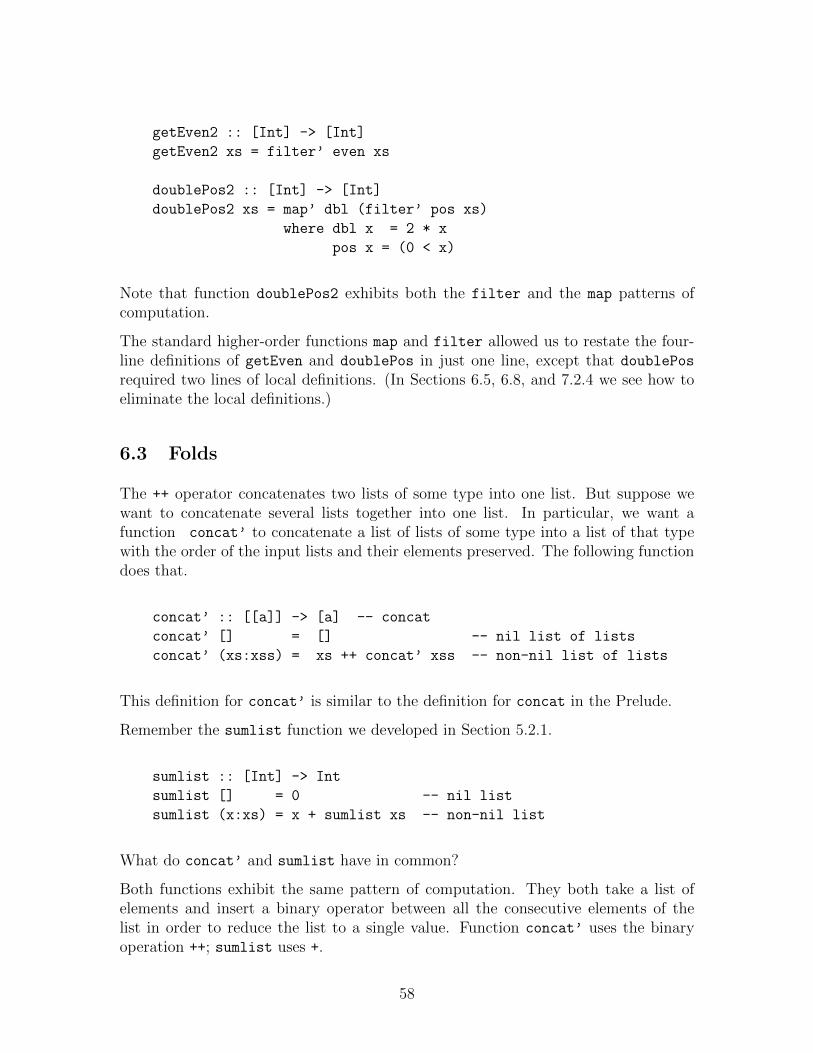
getEven2 :: [Int] -> [Int]

getEven2 xs = filter’ even xs

doublePos2 :: [Int] -> [Int]

doublePos2 xs = map’ dbl (filter’ pos xs)

where dbl x = 2 * x

pos x = (0 < x)

Note that function doublePos2 exhibits both the filter and the map patterns ofcomputation.

The standard higher-order functions map and filter allowed us to restate the four-line definitions of getEven and doublePos in just one line, except that doublePos

required two lines of local definitions. (In Sections 6.5, 6.8, and 7.2.4 we see how toeliminate the local definitions.)

6.3 Folds

The ++ operator concatenates two lists of some type into one list. But suppose wewant to concatenate several lists together into one list. In particular, we want afunction concat’ to concatenate a list of lists of some type into a list of that typewith the order of the input lists and their elements preserved. The following functiondoes that.

concat’ :: [[a]] -> [a] -- concat

concat’ [] = [] -- nil list of lists

concat’ (xs:xss) = xs ++ concat’ xss -- non-nil list of lists

This definition for concat’ is similar to the definition for concat in the Prelude.

Remember the sumlist function we developed in Section 5.2.1.

sumlist :: [Int] -> Int

sumlist [] = 0 -- nil list

sumlist (x:xs) = x + sumlist xs -- non-nil list

What do concat’ and sumlist have in common?

Both functions exhibit the same pattern of computation. They both take a list ofelements and insert a binary operator between all the consecutive elements of thelist in order to reduce the list to a single value. Function concat’ uses the binaryoperation ++; sumlist uses +.

58

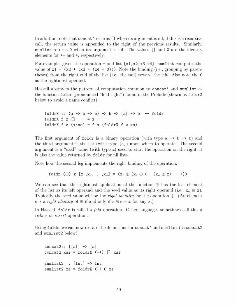
In addition, note that concat’ returns [] when its argument is nil; if this is a recursivecall, the return value is appended to the right of the previous results. Similarly,sumlist returns 0 when its argument is nil. The values [] and 0 are the identityelements for ++ and +, respectively.

For example, given the operation + and list [x1,x2,x3,x4], sumlist computes thevalue of x1 + (x2 + (x3 + (x4 + 0))). Note the binding (i.e., grouping by paren-theses) from the right end of the list (i.e., the tail) toward the left. Also note the 0

as the rightmost operand.

Haskell abstracts the pattern of computation common to concat’ and sumlist asthe function foldr (pronounced “fold right”) found in the Prelude (shown as foldrXbelow to avoid a name conflict).

foldrX :: (a -> b -> b) -> b -> [a] -> b -- foldr

foldrX f z [] = z

foldrX f z (x:xs) = f x (foldrX f z xs)

The first argument of foldr is a binary operation (with type a -> b -> b) andthe third argument is the list (with type [a]) upon which to operate. The secondargument is a “seed” value (with type a) used to start the operation on the right; itis also the value returned by foldr for nil lists.

Note how the second leg implements the right binding of the operation:

foldr (⊕) z [x1,x2,...,xn] = (x1 ⊕ (x2 ⊕ (· · · (xn ⊕ z) · · · )))

We can see that the rightmost application of the function ⊕ has the last elementof the list as its left operand and the seed value as its right operand (i.e., xn ⊕ z).Typically the seed value will be the right identity for the operation ⊕. (An elemente is a right identity of ⊕ if and only if x⊕ e = x for any x.)

In Haskell, foldr is called a fold operation. Other languages sometimes call this areduce or insert operation.

Using foldr, we can now restate the definitions for concat’ and sumlist (as concat2and sumlist2 below):

concat2:: [[a]] -> [a]

concat2 xss = foldrX (++) [] xss

sumlist2 :: [Int] -> Int

sumlist2 xs = foldrX (+) 0 xs

59

As further examples, consider the folding of the Boolean operators && (“and”) and ||

(“or”) over lists of Boolean values as Prelude functions and and or (shown as and’

and or’ below to avoid name conflicts):

and’, or’ :: [Bool] -> Bool -- and, or

and’ xs = foldrX (&&) True xs

or’ xs = foldrX (||) False xs

Although their definitions look different, and’ and or’ are actually identical to func-tions and and or in the Prelude.

As noted above, function foldr binds (i.e., groups by parentheses) the operation fromthe right toward the left. An alternative fold operation is one that binds from theleft toward the right. The foldl (pronounced “fold left”) function implements thiscomputational pattern. It uses the seed value to start the operation at the head ofthe list. Typically, the seed value will be the left identity of the operation.

The definition of foldl from the Prelude is similar to foldlX shown below:

foldlX :: (a -> b -> a) -> a -> [b] -> a -- foldl

foldlX f z [] = z

foldlX f z (x:xs) = foldlX f (f z x) xs

Note how the second leg of foldlX implements the left binding of the operation. Inthe recursive call of foldlX the “seed value” argument is used as an accumulatingparameter.

foldl (⊕) z [x1,x2,...,xn] = (· · · ((z ⊕ x1) ⊕ x2) ⊕ · · · xn)

Also note how the types of foldr and foldl differ.

If ⊕ is an associative binary operation of type t -> t -> t with identity element z

(i.e., a monoid), then:

foldr (⊕) z xs = foldl (⊕) z xs

Bird and Wadler call this property the first duality theorem [2].

Since both + and ++ are associative operations with identity elements, sumlist’ andconcat’’ can be implemented with either foldr or foldl.

Which is better?

Depending upon the nature of the operation, an implementation using foldr may bemore efficient than foldl or vice versa. We defer a more complete discussion of theefficiency until we study evaluation strategies in Section 13.

60

As a rule of thumb, however, if the operation ⊕ is nonstrict (see Section 6.4) in eitherargument, then it is usually better to use foldr. That form takes better advantageof lazy evaluation.

If the operation ⊕ is strict (see Section 6.4) in both arguments, then it is often better(i.e., more efficient) to use the optimized version of foldl called foldl’. We’ll discussthis more in Section 13.6.

As examples of the use of function foldl’ (from module Data.List), consider thefollowing functions, which are similar to sum and product in the Prelude (shownbelow as sum’ and product’ to avoid name conflicts):

sum’, product’ :: Num a => [a] -> a

sum’ xs = foldl’ (+) 0 xs -- sum

product’ xs = foldl’ (*) 1 xs -- product

Note that these functions can operate on lists of elements from some type in classNum.

6.4 Strictness

Some expressions cannot be reduced to a simple value, for example, 1/0. The at-tempted evaluation of such expressions either return an error immediately or causethe interpreter to go into an “infinite loop”.

In our discussions of functions, it is often convenient to assign the symbol ⊥ (pro-nounced “bottom”) as the value of expressions like 1/0. We use ⊥ is a polymorphicsymbol—as a value of every type.

The symbol⊥ is not in the Haskell syntax and the interpreter cannot actually generatethe value ⊥. It is merely a name for the value of an expression in situations wherethe expression cannot really be evaluated. It’s use is somewhat analogous to use ofsymbols such as ∞ in mathematics.

Although we cannot actually produce the value ⊥, we can, conceptually at least,apply any function to ⊥.

If f ⊥ = ⊥, then we say that the function is strict ; otherwise, it is nonstrict (some-times called lenient).

That is, a strict argument of a function must be evaluated before the final result canbe computed. A nonstrict argument of a function may not need to be evaluated tocompute the final result.

Assume that lazy evaluation is being used and consider the function two that takesan argument of any type and returns the integer value two.

61

two :: a -> Int

two x = 2

The function two is nonstrict. The argument expression is not evaluated to computethe final result. Hence, two ⊥ = 2.

Strict examples: Function rev (discussed in Section 5.4.2) is strict in its one argument.The arithmetic operations (e.g., +) are strict in both arguments.

Nonstrict examples: Operation ++ is strict in its first argument, but nonstrict in itssecond argument. Boolean functions && and || from the Prelude are also strict intheir first arguments and nonstrict in their second arguments.

(&&), (||) :: Bool -> Bool -> Bool

False && x = False -- second argument not evaluated

True && x = x

False || x = x

True || x = True -- second argument not evaluated

6.5 Currying and Partial Application

Consider the following two functions:

add :: (Int,Int) -> Int

add (x,y) = x + y

add’ :: Int -> (Int -> Int)

add’ x y = x + y

These functions are closely related, but they are not identical.

For all integers x and y, add (x,y) = add’ x y. But functions add and add’ havedifferent types.

Function add takes a 2-tuple (Int,Int) and returns an Int. Function add’ takes anInt and returns a function of type Int -> Int.

What is the result of the application add 3? An error.

What is the result of the application add’ 3? The result is a function that “adds 3to its argument”.

62

What is the result of the application (add’ 3) 4? The result is the integer value3 + 4.

By convention, function application (denoted by the juxtaposition of a function andits argument) binds to the left. That is, add’ x y = ((add’ x) y).

Hence, the higher-order functions in Haskell allow us to replace any function that takesa tuple argument by an equivalent function that takes a sequence of simple argumentscorresponding to the components of the tuple. This process is called currying. It isnamed after American logician Haskell B. Curry, who first exploited the technique.

Function add’ above is similar to the function (+) from the Prelude (i.e., the additionoperator).

We sometimes speak of the function (+) as being partially applied in the expression((+) 3). In this expression, the first argument of the function is “frozen in” and theresulting function can be passed as an argument, returned as a result, or applied toanother argument.

Partially applied functions are very useful in conjunction with other higher-orderfunctions.

For example, consider the partial applications of the relational comparison operator(<) and multiplication operator (*) in the function doublePos3. This function,which is equivalent to the function doublePos discussed in Section 6.2, doubles thepositive integers in a list:

doublePos3 :: [Int] -> [Int]

doublePos3 xs = map’ ((*) 2) (filter’ ((<) 0) xs)

Related to the notion of currying is the property of extensionality . Two functions f

and g are extensionally equal if f x = g x for all x.

Thus instead of writing the definition of g as

f, g :: a -> a

f x = some expression

g x = f x

we can write the definition of g as simply:

g = f

63

6.6 Operator Sections

Expressions such as ((*) 2) and ((<) 0), used in the definition of doublePos3 in theprevious subsection, can be a bit confusing because we normally use these operatorsin infix form. (In particular, it is difficult to remember the ((<) 0) returns True forpositive integers.)

Also, it would be helpful to be able to use the division operator to express a functionthat halves (i.e., divides by two) its operand? The function ((/) 2) does not do it;it divides 2 by its operand.

We can use the function flip from the Prelude to state the halving operation. Func-tion flip takes a function and two additional arguments and applies the argumentfunction to the two arguments with their order reversed. (This is show below asflip’ to avoid a name conflict.)

flip’ :: (a -> b -> c) -> b -> a -> c -- flip

flip’ f x y = f y x

Thus we can express the halving operator with the expression (flip (/) 2).

Because expressions such as ((<) 0) and (flip (/) 2) are quite common in pro-grams, Haskell provides a special, more compact and less confusing, syntax.

For some infix operator ⊕ and arbitrary expression e, expressions of the form (e⊕)and (⊕e) represent ((⊕) e) and (flip (⊕) e), respectively. Expressions of thisform are called operator sections.

Examples:

(1+) is the successor function, which returns the value of its argument plus 1.

(0<) is a test for a positive integer.

(/2) is the halving function.

(1.0/) is the reciprocal function.

(:[]) is the function that returns the singleton list containing the argument.

Suppose we want to sum the cubes of list of integers. We can express the function inthe following way:

sumCubes :: [Int] -> Int

sumCubes xs = sum’ (map’ (^3) xs)

64

Above ^ is the exponentiation operator and sum is the list summation function definedin the Prelude as:

sum = foldl’ (+) 0 -- sum

6.7 Combinators

The function flip in the previous subsection is an example of a useful type of functioncalled a combinator.

A combinator is a function without any free variables. That is, on right side of adefining equation there are no variables or operator symbols that are not bound onthe left side of the equation.

For historical reasons, flip is sometimes called the C combinator.

There are several other useful combinators in the Prelude.

The combinator const (shown below as const’) is the constant function constructor;it is a two-argument function that returns its first argument. For historical reasons,this combinator is sometimes called the K combinator.

const’ :: a -> b -> a -- const in Prelude

const’ k x = k

Example: (const 1) takes any argument and returns the value 1.

What does sum (map (const 1) xs) do?

Function id (shown below as id’) is the identity function; it is a one-argumentfunction that returns its argument unmodified. For historical reasons, this functionis sometimes called the I combinator.

id’ :: a -> a -- id in Prelude

id’ x = x

Combinators fst and snd (shown below as fst’ and snd’) extract the first andsecond components, respectively, of 2-tuples.

fst’ :: (a,b) -> a -- fst in Prelude

fst’ (x,_) = x

snd’ :: (a,b) -> b -- snd in Prelude

snd’ (_,y) = y

65

Similarly, fst3, snd3, and thd3 extract the first, second, and third components,respectively, of 3-tuples.

An interesting example that uses a combinator is the function reverse as defined inthe Prelude (shown below as reverse’):

reverse’ :: [a] -> [a] -- reverse in Prelude

reverse’ = foldlX (flip’ (:)) []

Function flip (:) takes a list on the left and an element on the right. As thisoperation is folded through the list from the left it attaches each element as the newhead of the list.

6.8 Functional Composition

The functional composition operator allows several “smaller” functions to be com-bined to form “larger” functions. In Haskell this combinator is denoted by the period(.) symbol and is defined in the Prelude as follows:

infixr 9 .

(.) :: (b -> c) -> (a -> b) -> (a -> c)

(f . g) x = f (g x)

Composition’s default binding is from the right and its precedence is higher than allthe operators we have discussed so far except function application itself.

Functional composition is an associative binary operation with the identity functionid as its identity element:

f . (g . h) = (f . g) . h

id . f = f . id

An advantage of the use of functional composition is that some expressions can bewritten more concisely. For example, the function

doit x = f1 (f2 (f3 (f4 x)))

can be written more concisely as

doit = f1 . f2 . f3 . f4

66

This form defines function doit as being equal to the composition of the other func-tions. It leaves the parameters of doit as implicit; doit has the same parameters asthe composition.

If doit is defined as above, then we can use the function in expressions such as map

(doit) xs. Of course, if this is the only use of the doit function, we can eliminate itcompletely and use the composition directly, e.g., map (f1 . f2 . f3 . f4) xs.

As an example, consider the function count that takes two arguments, an integern and a list of lists, and returns the number of the lists from the second argumentthat are of length n. Note that all functions composed below are single-argumentfunctions: length, (filter (== n)), (map length).

count :: Int -> [[a]] -> Int

count n

| n >= 0 = length . filter’ (== n) . map’ length

| otherwise = const’ 0 -- discard 2nd arg, return 0

Thus composition is a powerful form of “glue” that can be used to “stick” simplerfunctions together to build more powerful functions [14].

Remember the function doublePos that we discussed in Sections 6.2 and 6.5.

doublePos3 xs = map’ ((*) 2) (filter’ ((<) 0) xs)

Using composition and operator sections we can restate its definition as follows:

doublePos4 :: [Int] -> [Int]

doublePos4 = map’ (2*) . filter’ (0<)

Consider a function last to return the last element in a non-nil list and a functioninit to return the initial segment of a non-nil list (i.e., everything except the lastelement). These could quickly and concisely be written as follows:

last’ = head . reverse’ -- last in Prelude

init’ = reverse’ . tail . reverse’ -- init in Prelude

67

However, since these definitions are not very efficient, the Prelude implements func-tions last and init in a more direct and efficient way similar to the following:

last2 :: [a] -> a -- last in Prelude

last2 [x] = x

last2 (_:xs) = last2 xs

init2 :: [a] -> [a] -- init in Prelude

init2 [x] = []

init2 (x:xs) = x : init2 xs

The definitions for Prelude functions any and all are similar to the definitions showbelow; they take a predicate and a list and apply the predicate to each element of thelist, returning True when any and all, respectively, of the individual tests evaluate toTrue.

any’, all’ :: (a -> Bool) -> [a] -> Bool

any’ p = or’ . map’ p -- any in Prelude

all’ p = and’ . map’ p -- all in Prelude

The functions elem and notElem test for an object being an element of a list and notan element, respectively. They are defined in the Prelude similarly to the following:

elem’, notElem’ :: Eq a => a -> [a] -> Bool

elem’ = any’ . (==) -- elem in Prelude

notElem’ = all’ . (/=) -- notElem in Prelude

These are a bit more difficult to understand since any, all, ==, and /= are two-argument functions. Note that expression elem x xs would be evaluated as follows:

elem’ x xs

=⇒ { expand elem’ }(any’ . (==)) x xs

=⇒ { expand composition }any’ ((==) x) xs

The composition operator binds the first argument with (==) to construct the firstargument to any’. The second argument of any’ is the second argument of elem’.

68

6.9 Lambda Expressions

Remember the function squareAll2 we examined in the section on maps (Section 6.1):

squareAll2 :: [Int] -> [Int]

squareAll2 xs = map’ sq xs

where sq x = x * x

We introduced the local function definition sq to denote the function to be passed tomap. It seems to be a waste of effort to introduce a new symbol for a simple functionthat is only used in one place in an expression. Would it not be better, somehow, tojust give the defining expression itself in the argument position?

Haskell provides a mechanism to do just that, an anonymous function definition. Forhistorical reasons, these nameless functions are called lambda expressions. They beginwith a backslash \ and have the syntax:

\ atomicPatterns -> expression

For example, the squaring function (sq) could be replaced by a lambda expression as(\x -> x * x). The pattern x represents the single argument for this anonymousfunction and the expression x * x is its result.

A lambda expression to average two numbers is (\x y -> (x+y)/2).

An interesting example that uses a lambda expression is the function length asdefined in the Prelude—similar to length’ below. (Note that this uses the optimizedfunction foldl’ from the Data.List module.)

length’ :: [a] -> Int -- length in Prelude

length’ = foldl’ (\n _ -> n+1) 0

The anonymous function (\n _ -> n+1) takes an integer “counter” and a polymor-phic value and returns the “counter” incremented by one. As this function is foldedthrough the list from the left, this function counts each element of the second argu-ment.

6.10 List-Breaking Operations

In Section 5.5.2 we looked at the list-breaking functions take and drop. The Preludealso includes several higher-order list-breaking functions that take two arguments, apredicate that determines where the list is to be broken and the list to be broken.

69

The Prelude includes the functions span, break, takeWhile, dropWhile, takeUntil,and dropUntil.

Here we look at Prelude functions takeWhile and dropWhile. As you would expect,function takeWhile “takes” elements from the beginning of the list “while” the ele-ments satisfy the predicate and dropWhile “drops” elements from the beginning ofthe list “while” the elements satisfy the predicate. The Prelude definitions are similarto the following:

takeWhile’:: (a -> Bool) -> [a] -> [a] -- takeWhile

takeWhile’ p [] = []

takeWhile’ p (x:xs)

| p x = x : takeWhile’ p xs

| otherwise = []

dropWhile’ :: (a -> Bool) -> [a] -> [a] -- dropWhile

dropWhile’ p [] = []

dropWhile’ p xs@(x:xs’)

| p x = dropWhile’ p xs’

| otherwise = xs

Note the use of the pattern xs@(x:xs’) . This pattern matches a non-nil list with x

and xs’ binding to the head and tail, respectively, as usual. Variable xs binds to theentire list.

As an example, suppose we want to remove the leading blanks from a string. We cando that with the expression dropWhile ((==) ’ ’).

As with take and drop, the above functions can also be related by a “law”. For allfinite lists xs and predicates p on the same type:

takeWhile p xs ++ dropWhile p xs = xs

6.11 List-Combining Operations

In Section 5.5.3 we also looked at the function zip, which takes two lists and returnsa list of pairs of the corresponding elements. Function zip applies an operation, inthis case tuple-construction, to the corresponding elements of two lists.

We can generalize this pattern of computation with the function zipWith in whichthe operation is an argument to the function.

zipWith’ :: (a->b->c) -> [a]->[b]->[c] -- zipWith

zipWith’ z (x:xs) (y:ys) = z x y : zipWith’ z xs ys

zipWith’ _ _ _ = []

70

Using a lambda expression to state the tuple-forming operation, the Prelude defineszip in terms of zipWith:

zip’ :: [a] -> [b] -> [(a,b)]

zip’ = zipWith’ (\x y -> (x,y))

Or can be written more simply as:

zip’ :: [a] -> [b] -> [(a,b)]

zip’ = zipWith’ (,)

The zipWith function also enables us to define operations such as the scalar productof two vectors in a concise way.

sp :: Num a => [a] -> [a] -> a

sp xs ys = sum’ (zipWith’ (*) xs ys)

The Prelude includes versions of zipWith that take up to seven input lists: zipWith3· · · zipWith7.

71

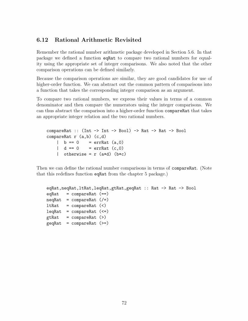
6.12 Rational Arithmetic Revisited

Remember the rational number arithmetic package developed in Section 5.6. In thatpackage we defined a function eqRat to compare two rational numbers for equal-ity using the appropriate set of integer comparisons. We also noted that the othercomparison operations can be defined similarly.

Because the comparison operations are similar, they are good candidates for use ofhigher-order function. We can abstract out the common pattern of comparisons intoa function that takes the corresponding integer comparison as an argument.

To compare two rational numbers, we express their values in terms of a commondenominator and then compare the numerators using the integer comparisons. Wecan thus abstract the comparison into a higher-order function compareRat that takesan appropriate integer relation and the two rational numbers.

compareRat :: (Int -> Int -> Bool) -> Rat -> Rat -> Bool

compareRat r (a,b) (c,d)

| b == 0 = errRat (a,0)

| d == 0 = errRat (c,0)

| otherwise = r (a*d) (b*c)

Then we can define the rational number comparisons in terms of compareRat. (Notethat this redefines function eqRat from the chapter 5 package.)

eqRat,neqRat,ltRat,leqRat,gtRat,geqRat :: Rat -> Rat -> Bool

eqRat = compareRat (==)

neqRat = compareRat (/=)

ltRat = compareRat (<)

leqRat = compareRat (<=)

gtRat = compareRat (>)

geqRat = compareRat (>=)

72

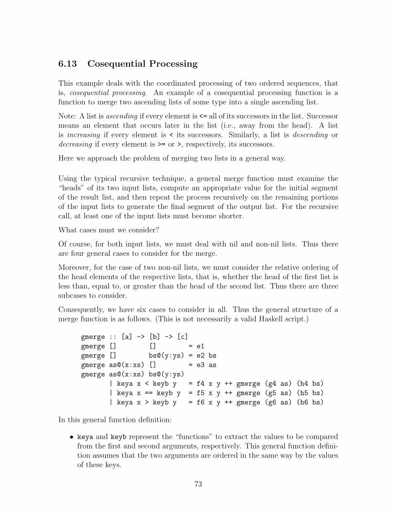
6.13 Cosequential Processing

This example deals with the coordinated processing of two ordered sequences, thatis, cosequential processing. An example of a cosequential processing function is afunction to merge two ascending lists of some type into a single ascending list.

Note: A list is ascending if every element is <= all of its successors in the list. Successormeans an element that occurs later in the list (i.e., away from the head). A listis increasing if every element is < its successors. Similarly, a list is descending ordecreasing if every element is >= or >, respectively, its successors.

Here we approach the problem of merging two lists in a general way.

Using the typical recursive technique, a general merge function must examine the“heads” of its two input lists, compute an appropriate value for the initial segmentof the result list, and then repeat the process recursively on the remaining portionsof the input lists to generate the final segment of the output list. For the recursivecall, at least one of the input lists must become shorter.

What cases must we consider?

Of course, for both input lists, we must deal with nil and non-nil lists. Thus thereare four general cases to consider for the merge.

Moreover, for the case of two non-nil lists, we must consider the relative ordering ofthe head elements of the respective lists, that is, whether the head of the first list isless than, equal to, or greater than the head of the second list. Thus there are threesubcases to consider.

Consequently, we have six cases to consider in all. Thus the general structure of amerge function is as follows. (This is not necessarily a valid Haskell script.)

gmerge :: [a] -> [b] -> [c]

gmerge [] [] = e1

gmerge [] bs@(y:ys) = e2 bs

gmerge as@(x:xs) [] = e3 as

gmerge as@(x:xs) bs@(y:ys)

| keya x < keyb y = f4 x y ++ gmerge (g4 as) (h4 bs)

| keya x == keyb y = f5 x y ++ gmerge (g5 as) (h5 bs)

| keya x > keyb y = f6 x y ++ gmerge (g6 as) (h6 bs)

In this general function definition:

• keya and keyb represent the “functions” to extract the values to be comparedfrom the first and second arguments, respectively. This general function defini-tion assumes that the two arguments are ordered in the same way by the valuesof these keys.

73

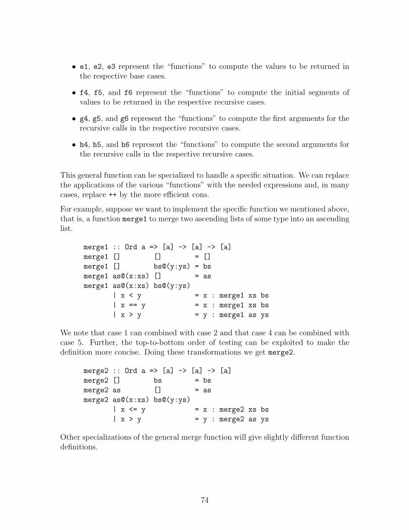
• e1, e2, e3 represent the “functions” to compute the values to be returned inthe respective base cases.

• f4, f5, and f6 represent the “functions” to compute the initial segments ofvalues to be returned in the respective recursive cases.

• g4, g5, and g6 represent the “functions” to compute the first arguments for therecursive calls in the respective recursive cases.

• h4, h5, and h6 represent the “functions” to compute the second arguments forthe recursive calls in the respective recursive cases.

This general function can be specialized to handle a specific situation. We can replacethe applications of the various “functions” with the needed expressions and, in manycases, replace ++ by the more efficient cons.

For example, suppose we want to implement the specific function we mentioned above,that is, a function merge1 to merge two ascending lists of some type into an ascendinglist.

merge1 :: Ord a => [a] -> [a] -> [a]

merge1 [] [] = []

merge1 [] bs@(y:ys) = bs

merge1 as@(x:xs) [] = as

merge1 as@(x:xs) bs@(y:ys)

| x < y = x : merge1 xs bs

| x == y = x : merge1 xs bs

| x > y = y : merge1 as ys

We note that case 1 can combined with case 2 and that case 4 can be combined withcase 5. Further, the top-to-bottom order of testing can be exploited to make thedefinition more concise. Doing these transformations we get merge2.

merge2 :: Ord a => [a] -> [a] -> [a]

merge2 [] bs = bs

merge2 as [] = as

merge2 as@(x:xs) bs@(y:ys)

| x <= y = x : merge2 xs bs

| x > y = y : merge2 as ys

Other specializations of the general merge function will give slightly different functiondefinitions.

74

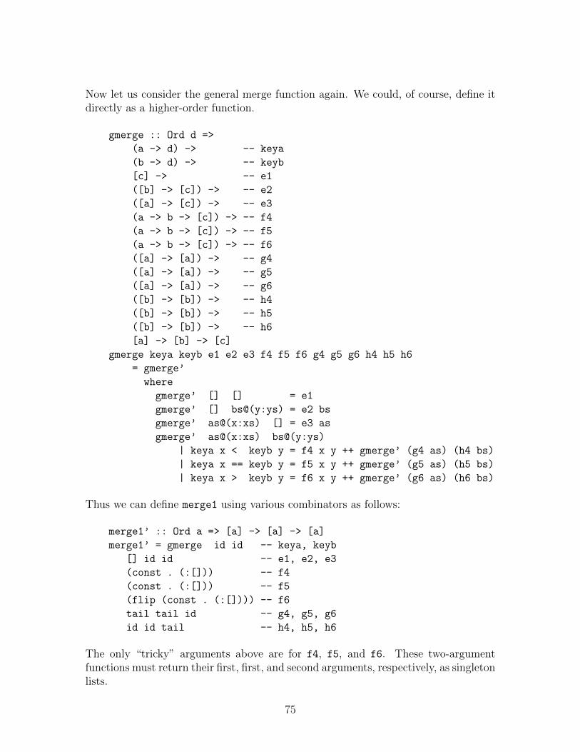
Now let us consider the general merge function again. We could, of course, define itdirectly as a higher-order function.

gmerge :: Ord d =>

(a -> d) -> -- keya

(b -> d) -> -- keyb

[c] -> -- e1

([b] -> [c]) -> -- e2

([a] -> [c]) -> -- e3

(a -> b -> [c]) -> -- f4

(a -> b -> [c]) -> -- f5

(a -> b -> [c]) -> -- f6

([a] -> [a]) -> -- g4

([a] -> [a]) -> -- g5

([a] -> [a]) -> -- g6

([b] -> [b]) -> -- h4

([b] -> [b]) -> -- h5

([b] -> [b]) -> -- h6

[a] -> [b] -> [c]

gmerge keya keyb e1 e2 e3 f4 f5 f6 g4 g5 g6 h4 h5 h6

= gmerge’

where

gmerge’ [] [] = e1

gmerge’ [] bs@(y:ys) = e2 bs

gmerge’ as@(x:xs) [] = e3 as

gmerge’ as@(x:xs) bs@(y:ys)

| keya x < keyb y = f4 x y ++ gmerge’ (g4 as) (h4 bs)

| keya x == keyb y = f5 x y ++ gmerge’ (g5 as) (h5 bs)

| keya x > keyb y = f6 x y ++ gmerge’ (g6 as) (h6 bs)

Thus we can define merge1 using various combinators as follows:

merge1’ :: Ord a => [a] -> [a] -> [a]

merge1’ = gmerge id id -- keya, keyb

[] id id -- e1, e2, e3

(const . (:[])) -- f4

(const . (:[])) -- f5

(flip (const . (:[]))) -- f6

tail tail id -- g4, g5, g6

id id tail -- h4, h5, h6

The only “tricky” arguments above are for f4, f5, and f6. These two-argumentfunctions must return their first, first, and second arguments, respectively, as singletonlists.

75

6.14 Exercises

1. Suppose you need a Haskell function times that takes a list of integers andreturns the product of the elements (e.g, times [2,3,4] returns 24). Writethe following versions as Haskell functions.

(a) A version that uses the Prelude function foldr.

(b) A version that uses backward recursion to compute the product. (Do notuse the list-folding Prelude functions such as foldr or product.)

(c) A version which uses forward recursion to compute the product. (Hint:use a tail-recursive auxiliary function with an accumulating parameter.)

2. For each of the following specifications, write a Haskell function that has thegiven arguments and result. Use the functions map, filter, and foldr asappropriate.

(a) Function numof takes a value and a list and returns the number of occur-rences of the value in the list.

(b) Function ellen takes a list of character strings and returns a list of thelengths of the corresponding strings.

(c) Function ssp takes a list of integers and returns the sum of the squares ofthe positive elements of the list.

3. Write a Haskell function map2 that takes a list of functions and a list of valuesand returns the list of results of applying each function in the first list to thecorresponding value in the second list.

4. Write a Haskell function fmap that takes a value and a list of functions andreturns the list of results from applying each function to the argument value.(For example, fmap 3 [((*) 2), ((+) 2)] yields [6,5].)

5. A list s is a prefix of a list t if there is some list u (perhaps nil) such that s ++

u == t. For example, the prefixes of string "abc" are "", "a", "ab", "abc".

A list s is a suffix of a list t if there is some list u (perhaps nil) such that u ++

s == t. For example, the suffixes of "abc" are "abc", "bc", "c", and "".

A list s is a segment of a list t if there are some (perhaps nil) lists u and v suchthat u ++ s ++ v == t. For example, the segments of string "abc" consist ofthe prefixes and the suffixes plus "b".

Write the following Haskell functions. You may use functions appearing earlyin the list to implement later ones.

(a) Write a function prefix such that prefix xs ys returns True if xs is aprefix of ys and returns False otherwise.

76

(b) Write a function suffixes such that suffixes xs returns the list of allsuffixes of list xs. (Hint: Generate them in the order given in the exampleof "abc" above.)

(c) Define a function indexes such that indexes xs ys returns a list of all thepositions at which list xs appears in list ys. Consider the first characterof ys as being at position 1. For example, indexes "ab" "abaabbab"

returns [1,4,7]. (Hint: Remember functions like map, filter, zip, andthe functions you just defined?)

(d) Define a function sublist such that sublist xs ys returns True if listxs appears as a segment of list ys and returns False otherwise.

6. Assume that the following Haskell type synonyms have been defined:

type Word = String -- word, characters left-to-right

type Line = [Word] -- line, words left-to-right

type Page = [Line] -- page, lines top-to-bottom

type Doc = [Page] -- document, pages front-to-back

Further assume that values of type Word do not contain any space characters.Implement the following Haskell text-handling functions:

(a) npages that takes a Doc and returns the number of Pages in the document.

(b) nlines that takes a Doc and returns the number of Lines in the document.

(c) nwords that takes a Doc and returns the number of Words in the document.

(d) nchars that takes a Doc and returns the number of Chars in the document(not including spaces of course).

(e) deblank that takes a Doc and returns the Doc with all blank lines removed.A blank line is a line that contains no words.

(f) linetext that takes a Line and returns the line as a String with the wordsappended together in left-to-right order separated by space characters andwith a newline character ’\n’ appended to the right end of the line. (Forexample, linetext ["Robert", "Khayat"] yields "Robert Khayat\n".)

(g) pagetext that takes a Page and returns the page as a String—applieslinetext to its component lines and appends the result in a top-to-bottomorder.

(h) doctext that takes a Doc and returns the document as a String—appliespagetext to its component lines and appends the result in a top-to-bottomorder.

(i) wordeq that takes a two Docs and returns True if the two documents areword equivalent and False otherwise. Two documents are word equivalentif they contain exactly the same words in exactly the same order regardlessof page and line structure. For example, [[["Robert"],["Khayat"]]] isword equivalent to [[["Robert","Khayat"]]].

77

78

7 MORE LIST NOTATION

7.1 Sequences

Haskell provides a compact notation for expressing arithmetic sequences.

An arithmetic sequence (or progression) is a sequence of elements from an enumer-ated type (i.e., a member of class Enum) such that consecutive elements have a fixeddifference. Int, Integer, Float, Double, and Char are all predefined members ofthis class.

• [m..n] produces the list of elements from m up to n in steps of one if m <= n;it produces the nil list otherwise.

Example: [1..5] =⇒ [1,2,3,4,5]

[5..1] =⇒ []

This feature is implemented with Prelude function enumFromTo applied as enumFromTom n.

• [m,m’..n] produces the list of elements from m in steps of m’-m. Note that ifm’ > m then the list is increasing up to n; if m’ < m then it is decreasing.

Example: [1,3..9] =⇒ [1,3,5,7,9]

[9,8..5] =⇒ [9,8,7,6,5]

[9,8..11] =⇒ []

This feature is implemented with Prelude function enumFromThenTo applied asenumFromThenTo m’ m n.

• [m..] and [m,m’..] produce potentially infinite lists beginning with m andhaving steps 1 and m’-m respectively.

These features are implemented with Prelude functions enumFrom applied asenumFrom m and enumFromThen applied as enumFromThen m m’.

Of course, we can provide our own functions for sequences. Consider the followingfunction to generate a geometric sequence.

A geometric sequence (or progression) is a sequence of elements from an ordered,numeric type (i.e., a member of both classes Ord and Num) such that consecutiveelements have a fixed ratio.

79

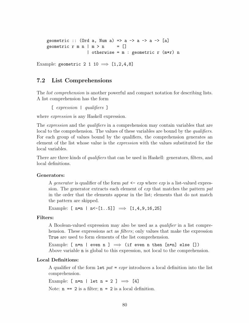
geometric :: (Ord a, Num a) => a -> a -> a -> [a]

geometric r m n | m > n = []

| otherwise = m : geometric r (m*r) n

Example: geometric 2 1 10 =⇒ [1,2,4,8]

7.2 List Comprehensions

The list comprehension is another powerful and compact notation for describing lists.A list comprehension has the form

[ expression | qualifiers ]

where expression is any Haskell expression.

The expression and the qualifiers in a comprehension may contain variables that arelocal to the comprehension. The values of these variables are bound by the qualifiers.For each group of values bound by the qualifiers, the comprehension generates anelement of the list whose value is the expression with the values substituted for thelocal variables.

There are three kinds of qualifiers that can be used in Haskell: generators, filters, andlocal definitions.

Generators:

A generator is qualifier of the form pat <- exp where exp is a list-valued expres-sion. The generator extracts each element of exp that matches the pattern patin the order that the elements appear in the list; elements that do not matchthe pattern are skipped.

Example: [ n*n | n<-[1..5]] =⇒ [1,4,9,16,25]

Filters:

A Boolean-valued expression may also be used as a qualifier in a list compre-hension. These expressions act as filters ; only values that make the expressionTrue are used to form elements of the list comprehension.

Example: [ n*n | even n ] =⇒ (if even n then [n*n] else [])

Above variable n is global to this expression, not local to the comprehension.

Local Definitions:

A qualifier of the form let pat = expr introduces a local definition into the listcomprehension.

Example: [ n*n | let n = 2 ] =⇒ [4]

Note: n == 2 is a filter; n = 2 is a local definition.

80

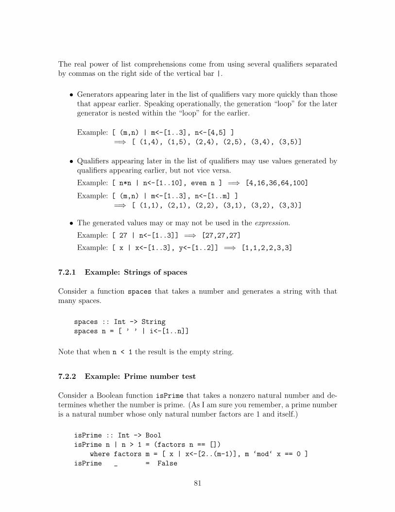
The real power of list comprehensions come from using several qualifiers separatedby commas on the right side of the vertical bar |.

• Generators appearing later in the list of qualifiers vary more quickly than thosethat appear earlier. Speaking operationally, the generation “loop” for the latergenerator is nested within the “loop” for the earlier.

Example: [ (m,n) | m<-[1..3], n<-[4,5] ]

=⇒ [ (1,4), (1,5), (2,4), (2,5), (3,4), (3,5)]

• Qualifiers appearing later in the list of qualifiers may use values generated byqualifiers appearing earlier, but not vice versa.

Example: [ n*n | n<-[1..10], even n ] =⇒ [4,16,36,64,100]

Example: [ (m,n) | m<-[1..3], n<-[1..m] ]

=⇒ [ (1,1), (2,1), (2,2), (3,1), (3,2), (3,3)]

• The generated values may or may not be used in the expression.

Example: [ 27 | n<-[1..3]] =⇒ [27,27,27]

Example: [ x | x<-[1..3], y<-[1..2]] =⇒ [1,1,2,2,3,3]

7.2.1 Example: Strings of spaces

Consider a function spaces that takes a number and generates a string with thatmany spaces.

spaces :: Int -> String

spaces n = [ ’ ’ | i<-[1..n]]

Note that when n < 1 the result is the empty string.

7.2.2 Example: Prime number test

Consider a Boolean function isPrime that takes a nonzero natural number and de-termines whether the number is prime. (As I am sure you remember, a prime numberis a natural number whose only natural number factors are 1 and itself.)

isPrime :: Int -> Bool

isPrime n | n > 1 = (factors n == [])

where factors m = [ x | x<-[2..(m-1)], m ‘mod‘ x == 0 ]

isPrime _ = False

81

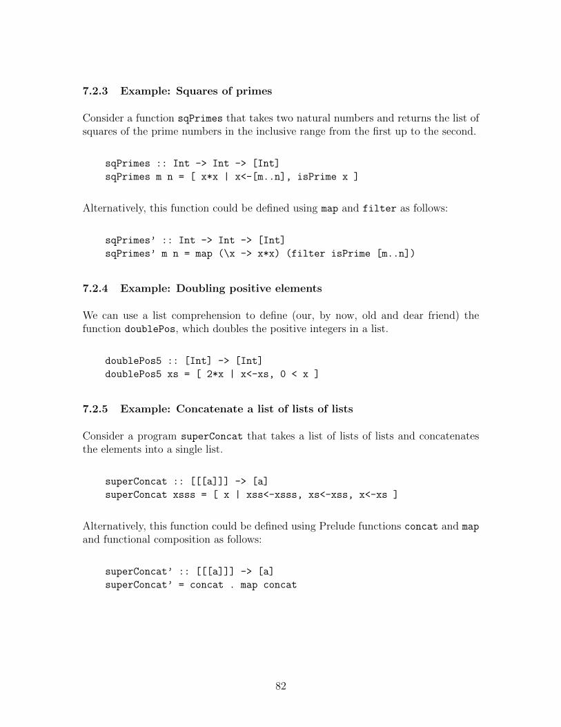
7.2.3 Example: Squares of primes

Consider a function sqPrimes that takes two natural numbers and returns the list ofsquares of the prime numbers in the inclusive range from the first up to the second.

sqPrimes :: Int -> Int -> [Int]

sqPrimes m n = [ x*x | x<-[m..n], isPrime x ]

Alternatively, this function could be defined using map and filter as follows:

sqPrimes’ :: Int -> Int -> [Int]

sqPrimes’ m n = map (\x -> x*x) (filter isPrime [m..n])

7.2.4 Example: Doubling positive elements

We can use a list comprehension to define (our, by now, old and dear friend) thefunction doublePos, which doubles the positive integers in a list.

doublePos5 :: [Int] -> [Int]

doublePos5 xs = [ 2*x | x<-xs, 0 < x ]

7.2.5 Example: Concatenate a list of lists of lists

Consider a program superConcat that takes a list of lists of lists and concatenatesthe elements into a single list.

superConcat :: [[[a]]] -> [a]

superConcat xsss = [ x | xss<-xsss, xs<-xss, x<-xs ]

Alternatively, this function could be defined using Prelude functions concat and map

and functional composition as follows:

superConcat’ :: [[[a]]] -> [a]

superConcat’ = concat . map concat

82

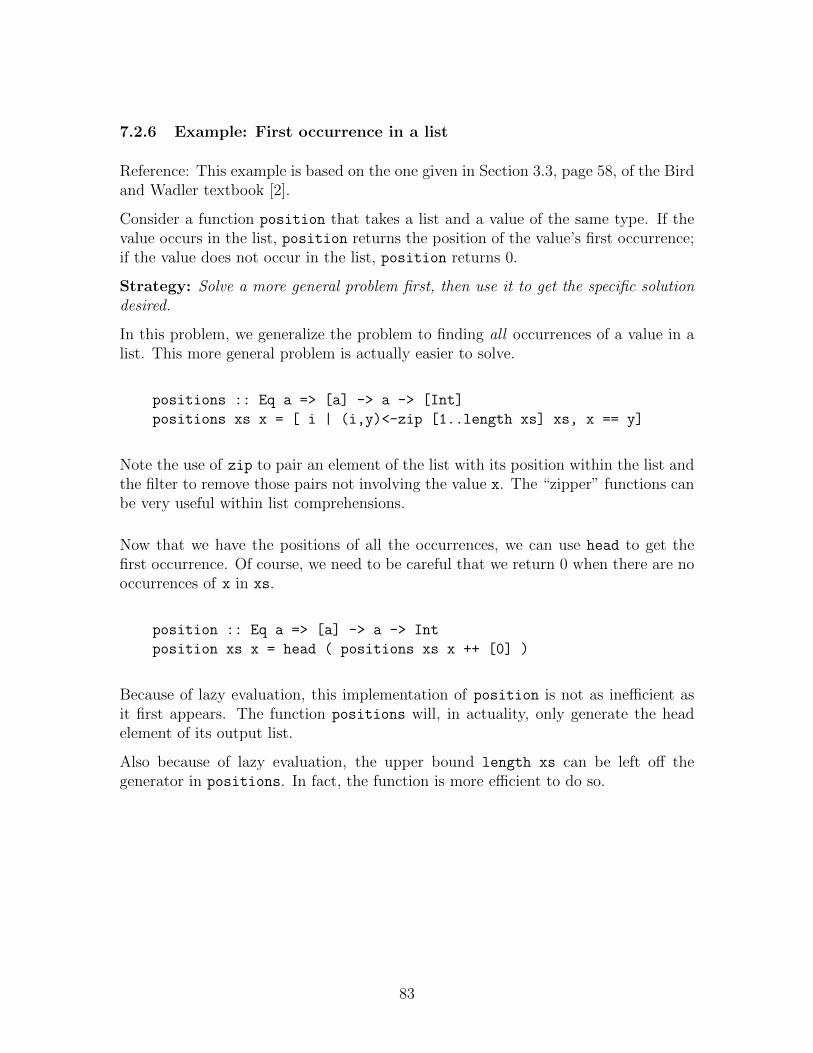
7.2.6 Example: First occurrence in a list

Reference: This example is based on the one given in Section 3.3, page 58, of the Birdand Wadler textbook [2].

Consider a function position that takes a list and a value of the same type. If thevalue occurs in the list, position returns the position of the value’s first occurrence;if the value does not occur in the list, position returns 0.

Strategy: Solve a more general problem first, then use it to get the specific solutiondesired.

In this problem, we generalize the problem to finding all occurrences of a value in alist. This more general problem is actually easier to solve.

positions :: Eq a => [a] -> a -> [Int]

positions xs x = [ i | (i,y)<-zip [1..length xs] xs, x == y]

Note the use of zip to pair an element of the list with its position within the list andthe filter to remove those pairs not involving the value x. The “zipper” functions canbe very useful within list comprehensions.

Now that we have the positions of all the occurrences, we can use head to get thefirst occurrence. Of course, we need to be careful that we return 0 when there are nooccurrences of x in xs.

position :: Eq a => [a] -> a -> Int

position xs x = head ( positions xs x ++ [0] )

Because of lazy evaluation, this implementation of position is not as inefficient asit first appears. The function positions will, in actuality, only generate the headelement of its output list.

Also because of lazy evaluation, the upper bound length xs can be left off thegenerator in positions. In fact, the function is more efficient to do so.

83

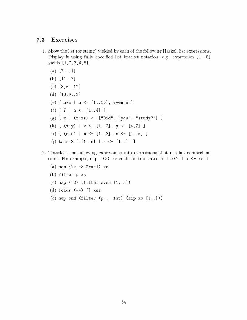
7.3 Exercises

1. Show the list (or string) yielded by each of the following Haskell list expressions.Display it using fully specified list bracket notation, e.g., expression [1..5]

yields [1,2,3,4,5].

(a) [7..11]

(b) [11..7]

(c) [3,6..12]

(d) [12,9..2]

(e) [ n*n | n <- [1..10], even n ]

(f) [ 7 | n <- [1..4] ]

(g) [ x | (x:xs) <- ["Did", "you", "study?"] ]

(h) [ (x,y) | x <- [1..3], y <- [4,7] ]

(i) [ (m,n) | m <- [1..3], n <- [1..m] ]

(j) take 3 [ [1..n] | n <- [1..] ]

2. Translate the following expressions into expressions that use list comprehen-sions. For example, map (*2) xs could be translated to [ x*2 | x <- xs ].

(a) map (\x -> 2*x-1) xs

(b) filter p xs

(c) map (^2) (filter even [1..5])

(d) foldr (++) [] xss

(e) map snd (filter (p . fst) (zip xs [1..]))

84

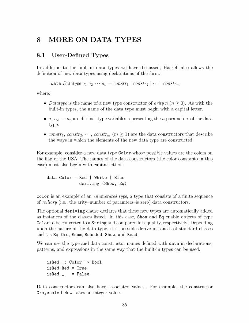
8 MORE ON DATA TYPES

8.1 User-Defined Types

In addition to the built-in data types we have discussed, Haskell also allows thedefinition of new data types using declarations of the form:

data Datatype a1 a2 · · · an = constr1 | constr2 | · · · | constrm

where:

• Datatype is the name of a new type constructor of arity n (n ≥ 0). As with thebuilt-in types, the name of the data type must begin with a capital letter.

• a1 a2 · · · an are distinct type variables representing the n parameters of the datatype.

• constr1, constr2, · · ·, constrm (m ≥ 1) are the data constructors that describethe ways in which the elements of the new data type are constructed.

For example, consider a new data type Color whose possible values are the colors onthe flag of the USA. The names of the data constructors (the color constants in thiscase) must also begin with capital letters.

data Color = Red | White | Blue

deriving (Show, Eq)

Color is an example of an enumerated type, a type that consists of a finite sequenceof nullary (i.e., the arity–number of paramters–is zero) data constructors.

The optional deriving clause declares that these new types are automatically addedas instances of the classes listed. In this case, Show and Eq enable objects of typeColor to be converted to a String and compared for equality, respectively. Dependingupon the nature of the data type, it is possible derive instances of standard classessuch as Eq, Ord, Enum, Bounded, Show, and Read.

We can use the type and data constructor names defined with data in declarations,patterns, and expressions in the same way that the built-in types can be used.

isRed :: Color -> Bool

isRed Red = True

isRed _ = False

Data constructors can also have associated values. For example, the constructorGrayscale below takes an integer value.

85

data Color’ = Red’ | Blue’ | Grayscale Int

deriving (Show, Eq)

Constructor Grayscale implicitly defines a constructor function with the typeInt -> Color’.

Consider a data type Point which has a type parameter. The following defines apolymorphic type; both of the values associated witha the constructor Pt must be oftype a. Constructor Pt implicitly defines a constructor function of type a -> a ->

Point a.

data Point a = Pt a a

deriving (Show, Eq)

A type like Point is often called a tuple type since it is essentially a Cartesian productof other types. Types like Color and Color’, which have multiple data constructors,are called (disjoint) union types.

As another example, consider a polymorphic set data type that represents a set as alist of values as follows. Note that the name Set is used both as the type constructorand a data constructor—in general, do not use a symbol in multiple ways.

data Set a = Set [a]

deriving (Show, Eq)

Now we can write a function makeSet to transform a list into a Set. This functionuses the funciton nub from the Data.List module to remove duplicates from a list.

makeSet :: Eq a => [a] -> Set a

makeSet xs = Set (nub xs)

As we have seen previously (Section 5.1), programmers can also define type synonyms.As in user-defined types, synonyms may have parameters. For example, the followingmight define a matrix of some polymorphic type as a list of lists of that type.

type Matrix a = [[a]]

We can also use special types to encode error conditions. For example, suppose wewant an integer division operation that returns an error message if there is an attemptto divide by 0 and returns the quotient otherwise. We can define and use a uniontype Result as follows:

86

data Result a = Ok a | Err String

deriving (Show, Eq)

divide :: Int -> Int -> Result Int

divide _ 0 = Err "Divide by zero"

divide x y = Ok (x ‘div‘ y)

Then we can use this operation in the definition of another function f that returnsthe maximum Int value maxBound when a division by 0 occurs.

f :: Int -> Int -> Int

f x y = return (divide x y)

where return (Ok z) = z

return (Err s) = maxBound

The auxiliary function return can be avoided by using the Haskell case expressionas follows:

f’ x y = case divide x y of

Ok z -> z

Err s -> maxBound

This case expression evaluates the expression divide x y, matches its result againstthe patterns of the alternatives, and returns the right-hand-side of the first matchingpattern.

8.2 Recursive Data Types

Types can also be recursive.

For example, consider the user-defined type BinTree, which defines a binary tree withvalues of a polymorphic type.

data BinTree a = Empty | Node (BinTree a) a (BinTree a)

deriving (Show, Eq)

This data type represents a binary tree with a value in each node. The tree is either“empty” (denoted by Empty) or it is a “node” (denoted by Node) that consists of avalue of type a and “left” and “right” subtrees. Each of the subtrees must themselvesbe objects of type BinTree.

Thus a binary tree is represented as a three-part “record” in which the left and rightsubtrees are represented as nested binary trees. There are no explicit “pointers”.

87

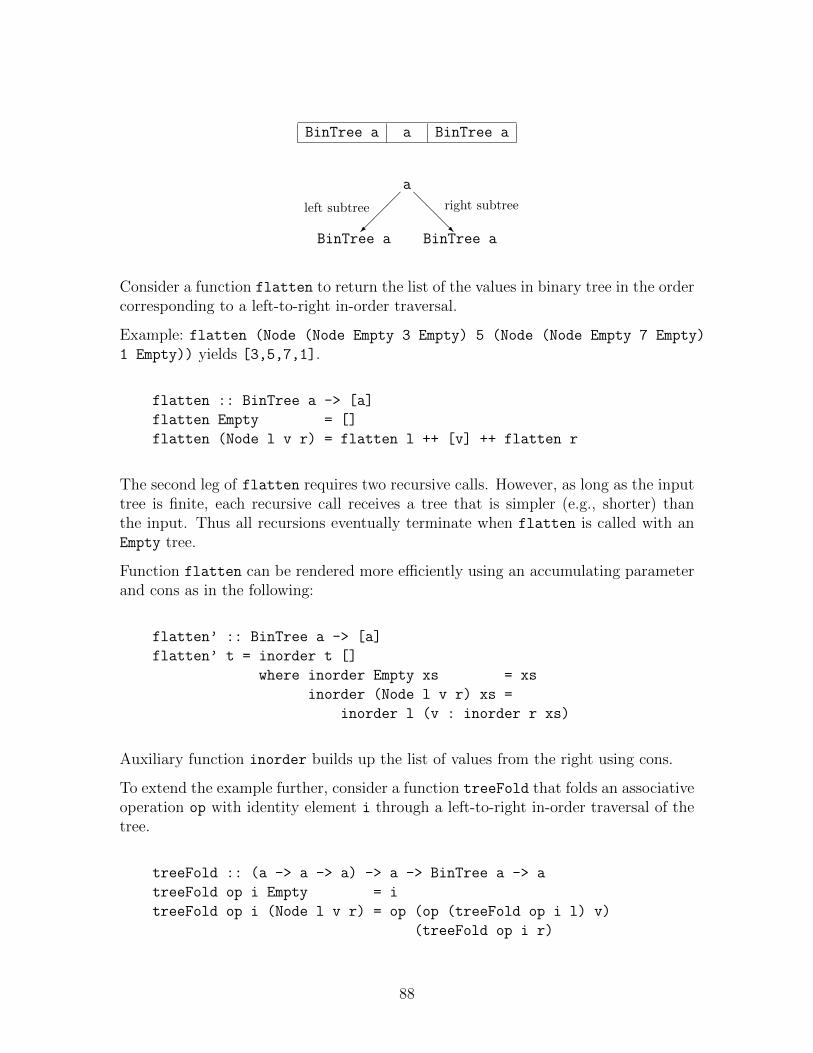
BinTree a a BinTree a

a�

��

left subtree

BinTree a

@@@R

right subtree

BinTree a

Consider a function flatten to return the list of the values in binary tree in the ordercorresponding to a left-to-right in-order traversal.

Example: flatten (Node (Node Empty 3 Empty) 5 (Node (Node Empty 7 Empty)

1 Empty)) yields [3,5,7,1].

flatten :: BinTree a -> [a]

flatten Empty = []

flatten (Node l v r) = flatten l ++ [v] ++ flatten r

The second leg of flatten requires two recursive calls. However, as long as the inputtree is finite, each recursive call receives a tree that is simpler (e.g., shorter) thanthe input. Thus all recursions eventually terminate when flatten is called with anEmpty tree.

Function flatten can be rendered more efficiently using an accumulating parameterand cons as in the following:

flatten’ :: BinTree a -> [a]

flatten’ t = inorder t []

where inorder Empty xs = xs

inorder (Node l v r) xs =

inorder l (v : inorder r xs)

Auxiliary function inorder builds up the list of values from the right using cons.

To extend the example further, consider a function treeFold that folds an associativeoperation op with identity element i through a left-to-right in-order traversal of thetree.

treeFold :: (a -> a -> a) -> a -> BinTree a -> a

treeFold op i Empty = i

treeFold op i (Node l v r) = op (op (treeFold op i l) v)

(treeFold op i r)

88

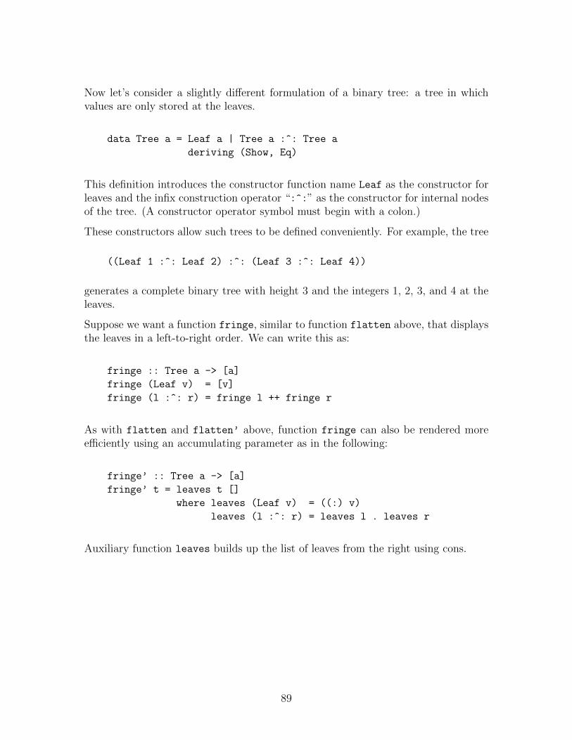
Now let’s consider a slightly different formulation of a binary tree: a tree in whichvalues are only stored at the leaves.

data Tree a = Leaf a | Tree a :^: Tree a

deriving (Show, Eq)

This definition introduces the constructor function name Leaf as the constructor forleaves and the infix construction operator “:^:” as the constructor for internal nodesof the tree. (A constructor operator symbol must begin with a colon.)

These constructors allow such trees to be defined conveniently. For example, the tree

((Leaf 1 :^: Leaf 2) :^: (Leaf 3 :^: Leaf 4))

generates a complete binary tree with height 3 and the integers 1, 2, 3, and 4 at theleaves.

Suppose we want a function fringe, similar to function flatten above, that displaysthe leaves in a left-to-right order. We can write this as:

fringe :: Tree a -> [a]

fringe (Leaf v) = [v]

fringe (l :^: r) = fringe l ++ fringe r

As with flatten and flatten’ above, function fringe can also be rendered moreefficiently using an accumulating parameter as in the following:

fringe’ :: Tree a -> [a]

fringe’ t = leaves t []

where leaves (Leaf v) = ((:) v)

leaves (l :^: r) = leaves l . leaves r

Auxiliary function leaves builds up the list of leaves from the right using cons.

89

8.3 Exercises

1. For trees of type Tree defined in Section 8.2, implement a tree-folding functionsimilar to treeFold.

2. For trees of type BinTree defined in Section 8.2, implement a version of treeFoldthat uses an accumulating parameter. (Hint: foldl.)

3. In a binary search tree all values in the left subtree of a node are less than thevalue at the node and all values in the right subtree are greater than the valueat the node. Given binary search trees of type BinTree defined in Section 8.2,implement the following Haskell functions:

makeTree that takes a list and returns a perfectly balanced (i.e., minimalheight) BinTree such that flatten (makeTree xs) = sort xs. Preludefunction sort returns its argument rearranged into ascending order.

insertTree that takes an element and a BinTree and returns the BinTree

with the element inserted at an appropriate position.

elemTree that takes an element and a BinTree and returns True if the elementis in the tree and False otherwise.

heightTree that takes a BinTree and returns its height. Assume that heightmeans the number of levels in the tree. (A tree consisting of exactly onenode has a height of 1.)

mirrorTree that takes a BinTree and returns its mirror image. That is, ittakes a tree and returns the tree with the left and right subtrees of everynode swapped.

mapTree that takes a function and a BinTree and returns the BinTree of thesame shape except each node’s value is computed by applying the functionto the corresponding value in the input tree.

showTree that takes a BinTree and displays the tree in a parenthesized, left-to-right, in-order traversal form. (That is, the traversal of a tree is enclosedin a pair of parentheses, with the traversal of the left subtree followed bythe traversal of the right subtree.)

Extend the package to support both insertion and deletion of elements. Keepthe tree balanced using a technique such the AVL balancing algorithm.

4. Implement the package of functions described in the previous exercise for thedata type Tree defined in Section 8.2.

90

5. Each node of a general (i.e., multiway) tree consists of a label and a list of (zeroor more) subtrees (each a general tree). We can define a general tree data typein Haskell as follows:

data Gtree a = Node a [Gtree a]

For example, tree (Node 0 [ ]) consists of a single node with label 0; a morecomplex tree, (Node 0 [ Node 1 [ ], Node 3 [ ], Node 7 [ ] ]), consistsof root node with three single-node subtrees.

Implement a “map” function for general trees, i.e., write Haskell function

mapGtree :: (a -> b) -> Gtree a -> Gtree b

that takes a function and a Gtree and returns the Gtree of the same shapesuch that each label is generated by applying the function to the correspondinglabel in the input tree.

6. We can introduce a new Haskell type for the natural numbers (i.e., nonnegativeintegers) with the statement

data Nat = Zero | Succ Nat

where the constructor Zero represents the value 0 and constructor Succ repre-sents the “successor function” from mathematics. Thus (Succ Zero) denotes 1,(Succ (Succ Zero)) denotes 2, and so forth. Implement the following Haskellfunctions.

intToNat that takes a nonnegative Int and returns the equivalent Nat, forexample, intToNat 2 returns (Succ (Succ Zero)).

natToInt that takes a Nat and returns the equivalent value of type Int, forexample, natToInt (Succ Zero) returns 1.

addNat that takes two Nats and returns their sum as a Nat. This functioncannot use integer addition.

mulNat that takes two Nats and returns their product as a Nat. This functioncannot use integer multiplication or addition.

compNat that takes two Nats and returns the value -1 if the first is less thanthe second, 0 if they are equal, and 1 if the first is greater than the second.This function cannot use the integer comparison operators.

91

7. Consider the following Haskell data type for representing sequences (i.e., lists):

data Seq a = Nil | Att (Seq a) a

Nil represents the empty sequence. Att xz y represents the sequence in whichlast element y is “attached” at the right end of the initial sequence xz.

Note that Att is similar to the ordinary “cons” for Haskell lists except that ele-ments are attached at the opposite end of the sequences. (Att (Att (Att Nil

1) 2) 3) represents the same sequence as the ordinary list (1:(2:(3:[]))).

Implement Haskell functions for the following operations on type Seq. The op-erations are analogous to the similarly named operations on the built-in Haskelllists.

lastSeq takes a nonempty Seq and returns its last (i.e., rightmost) element.

initialSeq takes a nonempty Seq and returns its initial sequence (i.e., se-quence remaining after the last element removed).

lenSeq takes a Seq and returns the number of elements that it contains.

headSeq takes a nonempty Seq and returns its head (i.e., leftmost) element.

tailSeq takes a nonempty Seq and returns the Seq remaining after the headelement is removed.

conSeq that takes an element and a Seq and returns a Seq with the argumentelement as its head and the Seq argument as its tail.

appSeq takes two arguments of type Seq and returns a Seq with the secondargument appended after the first.

revSeq takes a Seq and returns the Seq with the same elements in reverseorder.

mapSeq takes a function and a Seq and returns the Seq resulting from applyingthe function to each element of the sequence in turn.

filterSeq that takes a predicate and a Seq and returns the Seq containingonly those elements that satisfy the predicate.

listToSeq takes an ordinary Haskell list and returns the Seq with the samevalues in the same order (e.g., headSeq (listToSeq xs) = head xs fornonempty xs.)

seqToList takes a Seq and returns the ordinary Haskell list with the samevalues in the same order (e.g., head (seqToList xz) = headSeq xz fornonempty xz.)

92

8. Consider the following Haskell data type for representing sequences (i.e., lists):

data Seq a = Nil | Unit a | Cat (Seq a) (Seq a)

The constructor Nil represents the empty sequence; Unit represents a single-element sequence; and Cat represents the “concatenation” (i.e., append) of itstwo arguments, the second argument appended after the first.

Implement Haskell functions for the following operations on type Seq. The op-erations are analogous to the similarly named operations on the built-in Haskelllists. (Do not convert back and forth to lists.)

toSeq that takes a list and returns a corresponding Seq that is balanced.

fromSeq that takes a Seq and returns the corresponding list.

appSeq that takes two arguments of type Seq and returns a Seq with the secondargument appended after the first.

conSeq that takes an element and a Seq and returns a Seq with the argumentelement as its head and the Seq argument as its tail.

lenSeq that takes a Seq and returns the number of elements that it contains.

revSeq that takes a Seq and returns a Seq with the same elements in reverseorder.

headSeq that takes a nonempty Seq and returns its head (i.e., leftmost or front)element. (Be careful!)

tailSeq that takes a nonempty Seq and returns the Seq remaining after thehead is removed.

normSeq that takes a Seq and returns a Seq with unnecessary embedded Nilsremoved. (For example, normSeq (Cat (Cat Nil (Unit 1)) Nil) re-turns (Unit 1).)

eqSeq that takes two Seqs and returns True if the sequences of values areequal and returns False otherwise. Note that two Seq “trees” may bestructurally different yet represent the same sequence of values.

For example, (Cat Nil (Unit 1)) and (Cat (Unit 1) Nil) have thesame sequence of values (i.e., [1]). But (Cat (Unit 1) (Unit 2)) and(Cat (Unit 2) (Unit 1)) do not represent the same sequence of values(i.e., [1,2] and [2,1], respectively).

Also (Cat (Cat (Unit 1) (Unit 2)) (Unit 3)) has the same sequenceof values as (Cat (Cat (Unit 1) (Unit 2)) (Unit 3)) (i.e., [1,2,3]).

In general what are the advantages and disadvantages of representing lists thisway?

93

94

9 INPUT/OUTPUT

This section from the Gofer/Hugs Notes is obselete. It is left in until the HaskellNotes can be fully revised.

103

104

10 PROBLEM SOLVING

A bit of the instructor’s philosophy:

• Programming is the essence of computing science.

• Problem solving is the essence of programming.

10.1 Polya’s Insights

The mathematician George Polya (1887–1985), a Professor of Mathematics at Stan-ford University, said the following in the preface to his book Mathematical Discovery:On Understanding, Learning and Teaching Problem Solving [21].

Solving a problem means finding a way out of a difficulty, a way around anobstacle, attaining an aim which was not immediately attainable. Solvingproblems is the specific achievement of intelligence, and intelligence is thespecific gift of mankind: solving problems can be regarded as the mostcharacteristically human activity. . . .

Solving problems is a practical art, like swimming, or skiing, or playingthe piano: you learn it only by imitation and practice. . . . if you wish tolearn swimming you have to go into the water, and if you wish to becomea problem solver you have to solve problems.

If you wish to derive the most profit from your effort, look out for suchfeatures of a problem at hand as may be useful in handling the problemsto come. A solution that you have obtained by your own effort or onethat you have read or heard, but have followed with real interest andinsight, may become a pattern for you, a model that you can imitate withadvantage in solving similar problems. . . .

Our knowledge about any subject consists of information and know-how .If you have genuine bona fide experience of mathematical work on anylevel, elementary or advanced, there will be no doubt in your mind that,in mathematics, know-how is much more important than mere possessionof information. . . .

What is know-how in mathematics? The ability to solve problems—notmerely routine problems but problems requiring some degree of indepen-dence, judgment, originality, creativity. Therefore, the first and foremostduty . . . in teaching mathematics is to emphasize methodical work in prob-lem solving.

What Polya says for mathematics holds just as much for computing science.

105

In his book How to Solve It [20], Polya states four phases of problem solving. Thesesteps are important for programming as well.

1. Understand the problem.

2. Devise a plan.

3. Carry out the plan, checking each step.

4. Reexamine and reconsider the solution. (And, of course, reexamine the under-standing of the problem, the plan, and the way the plan was carried out.)

10.2 Problem-Solving Strategies

The Bird and Wadler textbook gives several examples of problem-solving strategiesthat are sometimes useful in functional programming (indeed all programming).

Solve a more general problem first. That is, solve a “harder” problem than thespecific problem at hand, then use the solution of the “harder” problem to getthe specific solution desired.

Sometimes a solution of the more general problem is actually easier to findbecause the problem is simpler to state or more symmetrical or less obscuredby special conditions. The general solution can often be used to solve otherrelated problems.

Often the solution of the more general problem can actually lead to a moreefficient solution of the specific problem.

Example: We have already seen one example of this technique: finding the firstoccurrence of an item in a list (page 58 of Bird/Wadler [2], page 83 of thesenotes).

First, we devised a program to find all occurrences in a list. Then we selectedthe first occurrence from the set of all occurrences. (Lazy evaluation of Haskellprograms means that this use of a more general solution differs very little inefficiency from a specialized version.)

Example: Another example from Bird/Wadler is the fast Fibonacci programon page 128. This program optimizes the efficiency of computing fib n bycomputing (fib n, fib (n+1)) instead. This is a harder problem, but itactually gives us more information to work with and, hence, provides moreopportunity for optimization.

106

Solve a simpler problem first. Then adapt or extend the solution to solve theoriginal problem.

Often the mass of details in a problem description makes seeing a solutiondifficult. In the previous technique we made the problem easier by finding amore general problem to solve. In this technique, we move in the other direction:we find a more specific problem that is similar and solve it.

At worst, by solving the simpler problem we should get a better understandingof the problem we really want to solve. The more familiar we are with a problem,the more information we have about it, and, hence, the more likely we will beable to solve it.

At best, by solving the simpler problem we will find a solution that can be easilyextended to build a solution to the original problem.

Example: Section 4.1 of Bird/Wadler gives an good example of the applicationof this technique. The problem is to convert a positive integer of up to six digitsto the English words for that number (e.g., 369027 becomes “three hundred andsixty-nine thousand and twenty-seven”).

To deal with the complexity of this problem, Bird and Wadler first simplifiesthe problem to converting a two-digit number to words. Once that is done, theyextend the solution to three digits, and then to six digits.

Reuse “off-the-shelf” solutions to standard subproblems. We have been do-ing this all during this semester, especially since we began began studying poly-morphism and higher-order functions.

The basic idea is to identify standard patterns of computation (e.g., standardprelude functions such as length, take, zip, map, filter, foldr) that willsolve some aspects of the problem and then combine these standard patternswith your own specialized functions to construct a solution to the problem.

Example: Section 4.2 of Bird/Wadler gives develops a package of functions to doarithmetic on variable length integers. The functions take advantage of severalof the standard prelude functions.

Solve a related problem. Then transform the solution of the related problem toget a solution to the original problem.

Perhaps we can find an entirely different problem formulation (i.e., stated indifferent terms) for which we can readily find a solution. Then that solutioncan be converted into a solution to the problem at hand.

For example, we may take some problem and recast it in terms of some math-ematical or logical framework, solve the corresponding problem in that frame-work, and then interpret the results for the original problem. The simplificationprovided by the framework may reveal solutions that are obscured in the details

107

of the problem. We can also take advantage of the theory and techniques thathave been found previously for the mathematical framework.

Example: The example given in Section 4.3 of the Bird and Wadler textbookis quite interesting. The problem is to develop a text processing package, inparticular a function to break a string of text up into a list of lines.

This is not trivial. However, the “inverse” problem is trivial. All that is neededto convert a list of lines to a string of text is to insert linefeed characters betweenthe lines.

The example proceeds by first solving the inverse problem (line-folding) andthen uses it to calculate what the line-breaking program must be.

Separate concerns. That is, partition the problem into logically separate problems,solve each problem separately, then combine the solutions to the subproblemsto construct a solution to the problem at hand.

As we have seen in the above strategies, when a problem is complex and difficultto attack directly, we search for simpler, but related, problems to solve, thenbuild a solution to the complex problem from the simpler problems.

Example: Section 4.5 of Bird/Wadler shows the development of a program toprint a calendar for any year. It approaches the problem by first separatingit into two independent subproblems: building a calendar and assembling apicture. After solving each of these simpler problems, the more complex problemcan be solved easily by combining the two solutions

Divide and conquer. This is a special case of the “solve a simpler problem first”strategy. In this technique, we must divide the problem into subproblems thatare the same as the original problem except that the size of the input is smaller.

This process of division continues recursively until we get a problem that canbe solved trivially, then we combined we reverse the process by combining thesolutions to subproblems to form solutions to larger problems.

Example: Section 6.4 of Bird/Wadler shows the development of divide andconquer programs for sorting and binary search.

There are, of course, other strategies that can be used to approach problem solving.

108

11 HASKELL “LAWS”

11.1 Stating and Proving Laws

In Section 1 we defined referential transparency to mean that, within some well-defined context, a variable (or other symbol) always represents the same value. Thisallows one expression to be replaced by an equivalent expression or, more informally,“equals to be replaced by equals” .

Referential transparency is probably the most important property of purely functionalprogramming languages like Haskell. It allows us to state and prove various “laws”or identities that hold for functions and to use these “laws”to transform programsinto equivalent ones.

We have already seen a number of these laws. Again consider the append operator(++) for finite lists .

infixr 5 ++

(++) :: [a] -> [a] -> [a]

[] ++ xs = xs -- append.1

(x:xs) ++ ys = x:(xs ++ ys) -- append.2

The append operator has two useful properties that we have already seen:

Associativity: For any finite lists xs, ys, and zs,xs ++ (ys ++ zs) = (xs ++ ys) ++ zs.

Identity: For any finite list xs, [] ++ xs = xs = xs ++ [].

Note: Thus append over a finite list forms a monoid.

How do we prove these properties?

The answer is, of course, induction. But we need a type of induction that allows usto prove theorems over the set of all finite lists. In fact, we have already been usingthis form of induction in the informal arguments that the list-processing functionsterminate.

Induction over the natural numbers is a special case of a more general form of induc-tion called structural induction. This type of induction is over the syntactic structureof recursively (inductively) defined objects. Such objects can be partially ordered bya complexity ordering from the most simple (minimal) to the more complex.

If we think about the usual axiomization of the natural numbers (i.e., Peano’s postu-lates), then we see that 0 is the only simple (minimal) object and that the successorfunction ((+) 1) is the only constructor.

109

In the case of finite lists, the only simple object is the nil list [] and the only con-structor is the cons operator.

To prove a proposition P(x) holds for any finite object x, one must prove the followingcases:

Base cases. That P(e) holds for each simple (minimal) object e.

Inductive cases. That, for all object constructors C, if P(x) holds for some arbitraryobject(s) x, then P(C(x)) also holds.

That is, we can assume P(x) holds, then prove that P(C(x)) holds. This showsthat the constructors preserve proposition P.

To prove a proposition P(xs) holds for any finite list xs, the above reduces to thefollowing cases:

Base case xs = []. That P([]) holds.

Inductive case xs = (a:as). That, if P(as) holds, then P(a:as) also holds.

One, often useful, strategy for discovering proofs of laws is the following:

• Determine whether induction is needed to prove the law. Some laws can beproved directly from the definitions and other previously proved laws.

• Carefully choose the induction variable (or variables).

• Identify the base and inductive cases.

• For each case, use simplification independently on each side of the equation.Often, it is best to start with the side that is the most complex.

Simplification means to substitute the right-hand side of a definition or theinduction hypothesis for some expression matching the left-hand side.

• Continue simplifying each expression as long as possible.

Often we can show that the two sides of an equation are the same or that simplemanipulations (perhaps using previously proved laws) will show that they arethe same.

• If necessary, identify subcases and prove each subcase independently.

A formal proof of a case should, in general, be shown as a calculation that transformsone side of the equation into the other by substitution of equals for equals. Thisformal proof can be constructed from the calculation suggested in the above strategy.

Now that we have the mathematical machinery we need, let’s prove that ++ is as-sociative for all finite lists. The following proofs assume that all arguments of thefunctions are defined.

110

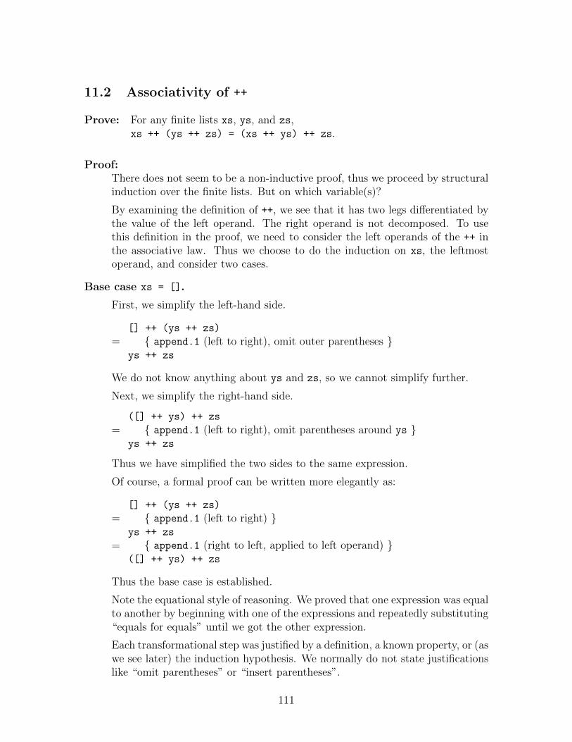
11.2 Associativity of ++

Prove: For any finite lists xs, ys, and zs,xs ++ (ys ++ zs) = (xs ++ ys) ++ zs.

Proof:There does not seem to be a non-inductive proof, thus we proceed by structuralinduction over the finite lists. But on which variable(s)?

By examining the definition of ++, we see that it has two legs differentiated bythe value of the left operand. The right operand is not decomposed. To usethis definition in the proof, we need to consider the left operands of the ++ inthe associative law. Thus we choose to do the induction on xs, the leftmostoperand, and consider two cases.

Base case xs = [].

First, we simplify the left-hand side.

[] ++ (ys ++ zs)

= { append.1 (left to right), omit outer parentheses }ys ++ zs

We do not know anything about ys and zs, so we cannot simplify further.

Next, we simplify the right-hand side.

([] ++ ys) ++ zs

= { append.1 (left to right), omit parentheses around ys }ys ++ zs

Thus we have simplified the two sides to the same expression.

Of course, a formal proof can be written more elegantly as:

[] ++ (ys ++ zs)

= { append.1 (left to right) }ys ++ zs

= { append.1 (right to left, applied to left operand) }([] ++ ys) ++ zs

Thus the base case is established.

Note the equational style of reasoning. We proved that one expression was equalto another by beginning with one of the expressions and repeatedly substituting“equals for equals” until we got the other expression.

Each transformational step was justified by a definition, a known property, or (aswe see later) the induction hypothesis. We normally do not state justificationslike “omit parentheses” or “insert parentheses”.

111

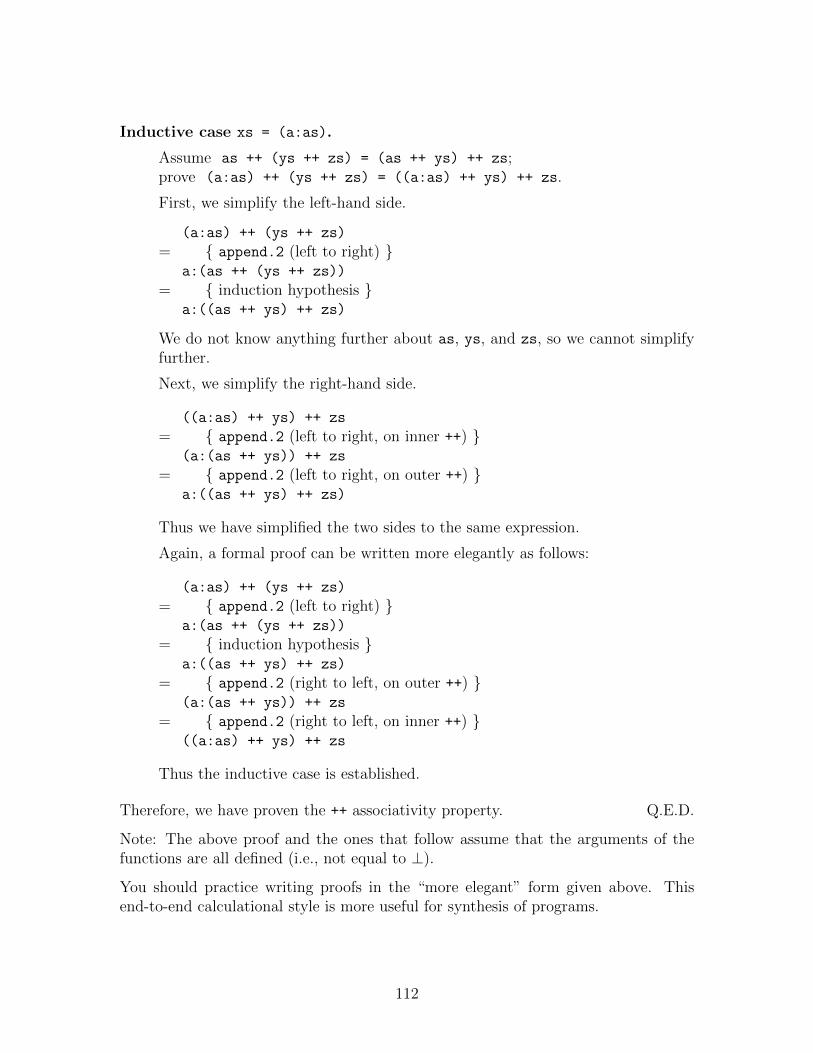
Inductive case xs = (a:as).

Assume as ++ (ys ++ zs) = (as ++ ys) ++ zs;prove (a:as) ++ (ys ++ zs) = ((a:as) ++ ys) ++ zs.

First, we simplify the left-hand side.

(a:as) ++ (ys ++ zs)

= { append.2 (left to right) }a:(as ++ (ys ++ zs))

= { induction hypothesis }a:((as ++ ys) ++ zs)

We do not know anything further about as, ys, and zs, so we cannot simplifyfurther.

Next, we simplify the right-hand side.

((a:as) ++ ys) ++ zs

= { append.2 (left to right, on inner ++) }(a:(as ++ ys)) ++ zs

= { append.2 (left to right, on outer ++) }a:((as ++ ys) ++ zs)

Thus we have simplified the two sides to the same expression.

Again, a formal proof can be written more elegantly as follows:

(a:as) ++ (ys ++ zs)

= { append.2 (left to right) }a:(as ++ (ys ++ zs))

= { induction hypothesis }a:((as ++ ys) ++ zs)

= { append.2 (right to left, on outer ++) }(a:(as ++ ys)) ++ zs

= { append.2 (right to left, on inner ++) }((a:as) ++ ys) ++ zs

Thus the inductive case is established.

Therefore, we have proven the ++ associativity property. Q.E.D.

Note: The above proof and the ones that follow assume that the arguments of thefunctions are all defined (i.e., not equal to ⊥).

You should practice writing proofs in the “more elegant” form given above. Thisend-to-end calculational style is more useful for synthesis of programs.

112

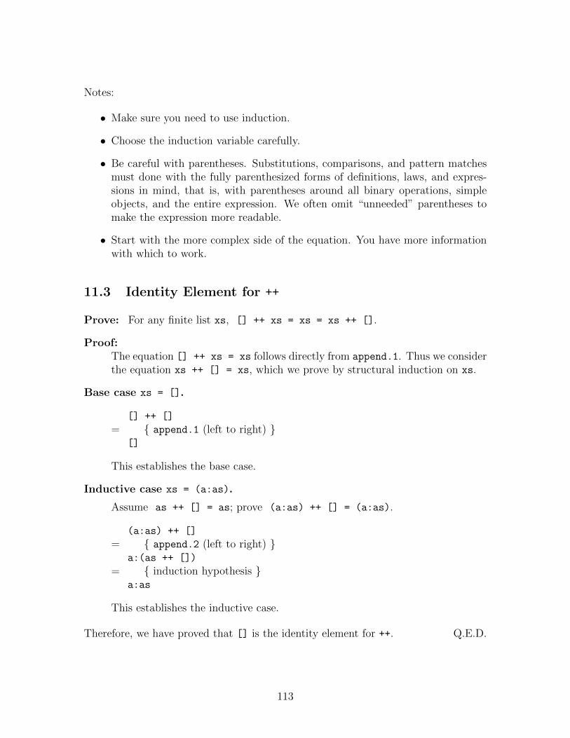
Notes:

• Make sure you need to use induction.

• Choose the induction variable carefully.

• Be careful with parentheses. Substitutions, comparisons, and pattern matchesmust done with the fully parenthesized forms of definitions, laws, and expres-sions in mind, that is, with parentheses around all binary operations, simpleobjects, and the entire expression. We often omit “unneeded” parentheses tomake the expression more readable.

• Start with the more complex side of the equation. You have more informationwith which to work.

11.3 Identity Element for ++

Prove: For any finite list xs, [] ++ xs = xs = xs ++ [].

Proof:The equation [] ++ xs = xs follows directly from append.1. Thus we considerthe equation xs ++ [] = xs, which we prove by structural induction on xs.

Base case xs = [].

[] ++ []

= { append.1 (left to right) }[]

This establishes the base case.

Inductive case xs = (a:as).

Assume as ++ [] = as; prove (a:as) ++ [] = (a:as).

(a:as) ++ []

= { append.2 (left to right) }a:(as ++ [])

= { induction hypothesis }a:as

This establishes the inductive case.

Therefore, we have proved that [] is the identity element for ++. Q.E.D.

113

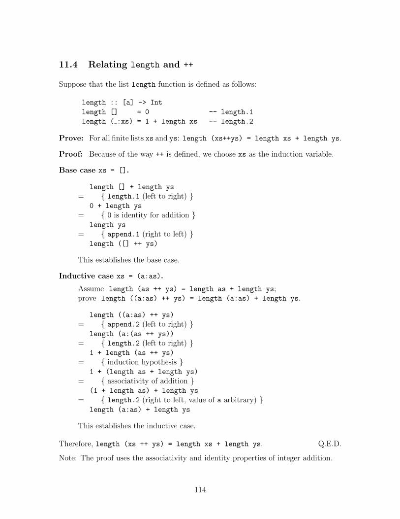
11.4 Relating length and ++

Suppose that the list length function is defined as follows:

length :: [a] -> Int

length [] = 0 -- length.1

length ( :xs) = 1 + length xs -- length.2

Prove: For all finite lists xs and ys: length (xs++ys) = length xs + length ys.

Proof: Because of the way ++ is defined, we choose xs as the induction variable.

Base case xs = [].

length [] + length ys

= { length.1 (left to right) }0 + length ys

= { 0 is identity for addition }length ys

= { append.1 (right to left) }length ([] ++ ys)

This establishes the base case.

Inductive case xs = (a:as).

Assume length (as ++ ys) = length as + length ys;prove length ((a:as) ++ ys) = length (a:as) + length ys.

length ((a:as) ++ ys)

= { append.2 (left to right) }length (a:(as ++ ys))

= { length.2 (left to right) }1 + length (as ++ ys)

= { induction hypothesis }1 + (length as + length ys)

= { associativity of addition }(1 + length as) + length ys

= { length.2 (right to left, value of a arbitrary) }length (a:as) + length ys

This establishes the inductive case.

Therefore, length (xs ++ ys) = length xs + length ys. Q.E.D.

Note: The proof uses the associativity and identity properties of integer addition.

114

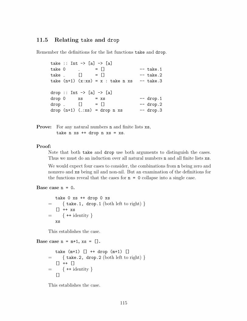
11.5 Relating take and drop

Remember the definitions for the list functions take and drop.

take :: Int -> [a] -> [a]

take 0 = [] -- take.1

take [] = [] -- take.2

take (n+1) (x:xs) = x : take n xs -- take.3

drop :: Int -> [a] -> [a]

drop 0 xs = xs -- drop.1

drop [] = [] -- drop.2

drop (n+1) ( :xs) = drop n xs -- drop.3

Prove: For any natural numbers n and finite lists xs,take n xs ++ drop n xs = xs.

Proof:Note that both take and drop use both arguments to distinguish the cases.Thus we must do an induction over all natural numbers n and all finite lists xs.

We would expect four cases to consider, the combinations from n being zero andnonzero and xs being nil and non-nil. But an examination of the definitions forthe functions reveal that the cases for n = 0 collapse into a single case.

Base case n = 0.

take 0 xs ++ drop 0 xs

= { take.1, drop.1 (both left to right) }[] ++ xs

= { ++ identity }xs

This establishes the case.

Base case n = m+1, xs = [].

take (m+1) [] ++ drop (m+1) []

= { take.2, drop.2 (both left to right) }[] ++ []

= { ++ identity }[]

This establishes the case.

115

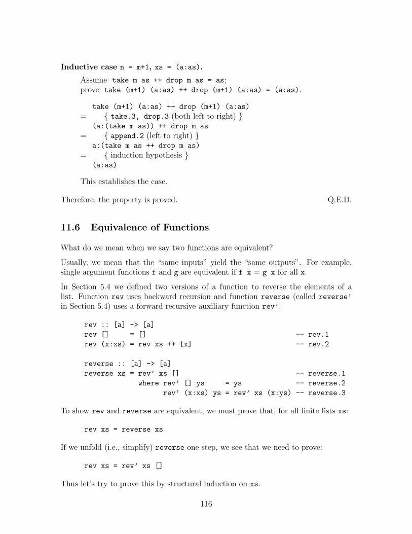
Inductive case n = m+1, xs = (a:as).

Assume take m as ++ drop m as = as;prove take (m+1) (a:as) ++ drop (m+1) (a:as) = (a:as).

take (m+1) (a:as) ++ drop (m+1) (a:as)

= { take.3, drop.3 (both left to right) }(a:(take m as)) ++ drop m as

= { append.2 (left to right) }a:(take m as ++ drop m as)

= { induction hypothesis }(a:as)

This establishes the case.

Therefore, the property is proved. Q.E.D.

11.6 Equivalence of Functions

What do we mean when we say two functions are equivalent?

Usually, we mean that the “same inputs” yield the “same outputs”. For example,single argument functions f and g are equivalent if f x = g x for all x.

In Section 5.4 we defined two versions of a function to reverse the elements of alist. Function rev uses backward recursion and function reverse (called reverse’

in Section 5.4) uses a forward recursive auxiliary function rev’.

rev :: [a] -> [a]

rev [] = [] -- rev.1

rev (x:xs) = rev xs ++ [x] -- rev.2

reverse :: [a] -> [a]

reverse xs = rev’ xs [] -- reverse.1

where rev’ [] ys = ys -- reverse.2

rev’ (x:xs) ys = rev’ xs (x:ys) -- reverse.3

To show rev and reverse are equivalent, we must prove that, for all finite lists xs:

rev xs = reverse xs

If we unfold (i.e., simplify) reverse one step, we see that we need to prove:

rev xs = rev’ xs []

Thus let’s try to prove this by structural induction on xs.

116

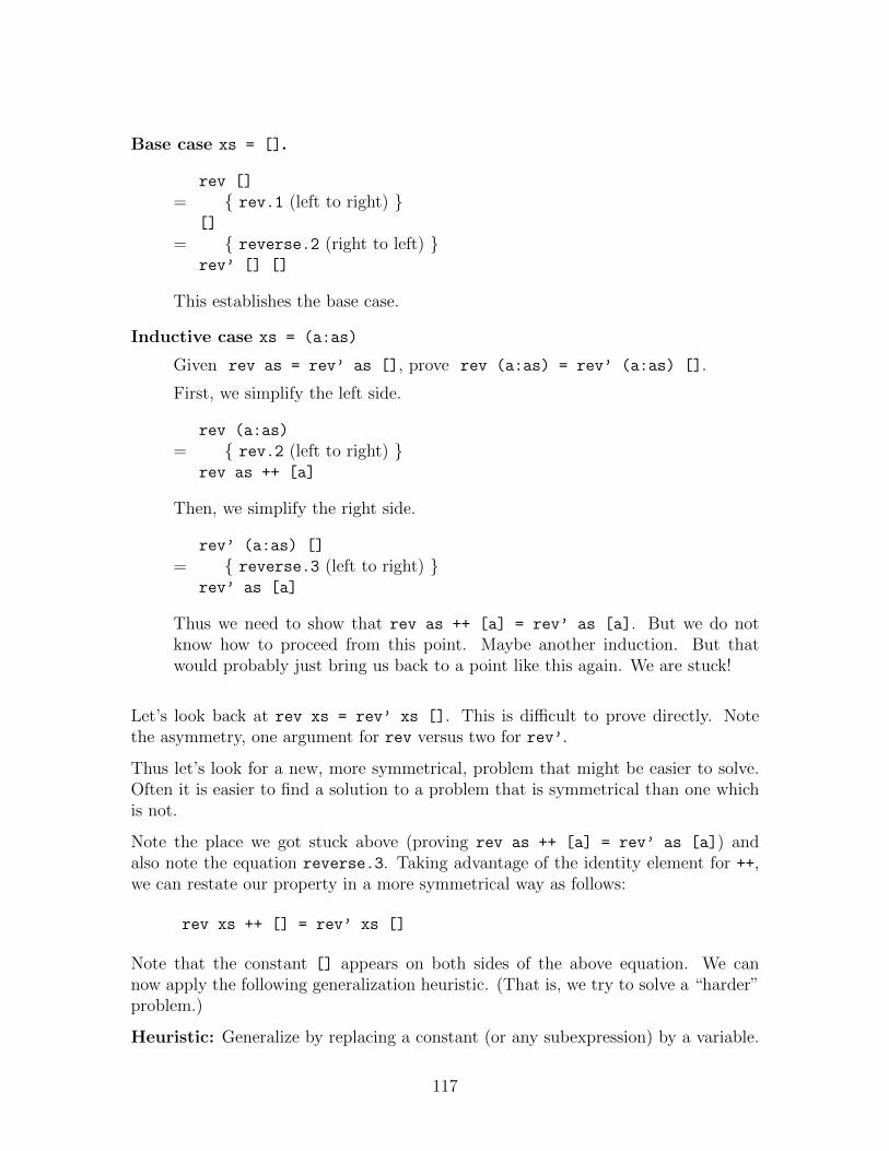
Base case xs = [].

rev []

= { rev.1 (left to right) }[]

= { reverse.2 (right to left) }rev’ [] []

This establishes the base case.

Inductive case xs = (a:as)

Given rev as = rev’ as [], prove rev (a:as) = rev’ (a:as) [].

First, we simplify the left side.

rev (a:as)

= { rev.2 (left to right) }rev as ++ [a]

Then, we simplify the right side.

rev’ (a:as) []

= { reverse.3 (left to right) }rev’ as [a]

Thus we need to show that rev as ++ [a] = rev’ as [a]. But we do notknow how to proceed from this point. Maybe another induction. But thatwould probably just bring us back to a point like this again. We are stuck!

Let’s look back at rev xs = rev’ xs []. This is difficult to prove directly. Notethe asymmetry, one argument for rev versus two for rev’.

Thus let’s look for a new, more symmetrical, problem that might be easier to solve.Often it is easier to find a solution to a problem that is symmetrical than one whichis not.

Note the place we got stuck above (proving rev as ++ [a] = rev’ as [a]) andalso note the equation reverse.3. Taking advantage of the identity element for ++,we can restate our property in a more symmetrical way as follows:

rev xs ++ [] = rev’ xs []

Note that the constant [] appears on both sides of the above equation. We cannow apply the following generalization heuristic. (That is, we try to solve a “harder”problem.)

Heuristic: Generalize by replacing a constant (or any subexpression) by a variable.

117

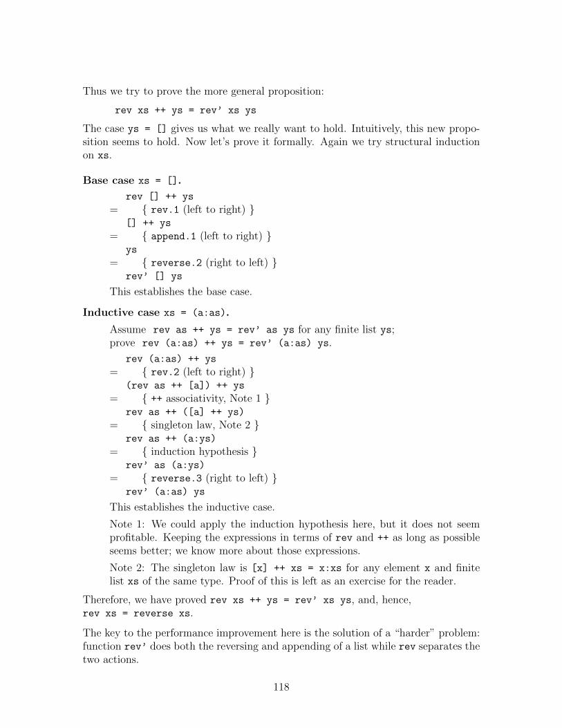
Thus we try to prove the more general proposition:

rev xs ++ ys = rev’ xs ys

The case ys = [] gives us what we really want to hold. Intuitively, this new propo-sition seems to hold. Now let’s prove it formally. Again we try structural inductionon xs.

Base case xs = [].

rev [] ++ ys

= { rev.1 (left to right) }[] ++ ys

= { append.1 (left to right) }ys

= { reverse.2 (right to left) }rev’ [] ys

This establishes the base case.

Inductive case xs = (a:as).

Assume rev as ++ ys = rev’ as ys for any finite list ys;prove rev (a:as) ++ ys = rev’ (a:as) ys.

rev (a:as) ++ ys

= { rev.2 (left to right) }(rev as ++ [a]) ++ ys

= { ++ associativity, Note 1 }rev as ++ ([a] ++ ys)

= { singleton law, Note 2 }rev as ++ (a:ys)

= { induction hypothesis }rev’ as (a:ys)

= { reverse.3 (right to left) }rev’ (a:as) ys

This establishes the inductive case.

Note 1: We could apply the induction hypothesis here, but it does not seemprofitable. Keeping the expressions in terms of rev and ++ as long as possibleseems better; we know more about those expressions.

Note 2: The singleton law is [x] ++ xs = x:xs for any element x and finitelist xs of the same type. Proof of this is left as an exercise for the reader.

Therefore, we have proved rev xs ++ ys = rev’ xs ys, and, hence,rev xs = reverse xs.

The key to the performance improvement here is the solution of a “harder” problem:function rev’ does both the reversing and appending of a list while rev separates thetwo actions.

118

11.7 Exercises

1. Prove for all x of some type and finite lists xs of the same type (singleton law):

[x] ++ xs = (x:xs)

2. Consider the definition for length given in Section 5.2.2 and the followingdefinition for len:

len :: Int -> [a] -> Int

len n [ ] = n -- len.1

len n ( :xs) = len (n+1) xs -- len.2

Prove for any finite list xs: len 0 xs = length xs.

3. Prove for all finite lists xs and ys of the same type:

reverse (xs ++ ys) = reverse ys ++ reverse xs

Hint: The function reverse (called reverse’ in Section 5.4) uses forward re-cursion. Backward recursive definitions are generally easier to use in inductiveproofs. In Section 5.4 we also defined a backward recursive function rev andproved that rev xs = reverse xs for all finite lists xs. Thus, you may find iteasier to substitute rev for reverse and instead prove:

rev (xs ++ ys) = rev ys ++ rev xs

4. Prove for all finite lists xs of some type: reverse (reverse xs) = xs

5. Prove for all natural numbers m and n and all finite lists xs:

drop n (drop m xs) = drop (m+n) xs

6. Consider the rational number package from Section 5.6. Prove for any BigRat

value r:

addRat r (0,1) = normRat r = addRat (0,1) r

7. Consider the two definitions for the Fibonacci function in Section 5.4.6. Provefor any natural number n:

fib n = fib’ n

Hint: First prove, for n ≥ 2:

fib’’ n p q = fib’’ (n-2) p q + fib’’ (n-1) p q

8. Prove that function id is the identity element of functional composition.

119

9. Prove that functional composition is associative.

10. Prove for all finite lists xs and ys of the same type and function f on that type:

map f (xs ++ ys) = map f xs ++ map f ys

11. Prove for all finite lists xs and ys of the same type and predicate p on thattype:

filter p (xs ++ ys) = filter p xs ++ filter p ys

12. Prove for all finite lists xs and ys of the same type and all predicates p on thattype:

all p (xs ++ ys) = (all p xs) && (all p ys)

Note: (&&) :: Bool -> Bool -> Bool

False && x = False -- second argument not evaluated

True && x = x

13. Prove for all finite lists xs of some type and predicates p and q on that type:

filter p (filter q xs) = filter q (filter p xs)

14. Prove for all finite lists xs and ys of the same type and for all functions f andvalues a of compatible types:

foldr f a (xs ++ ys) = foldr f (foldr f a ys) xs

15. Prove for all finite lists xs of some type and all functions f and g of conformingtypes:

map (f . g) xs = (map f . map g) xs

16. Prove for all finite lists of finite lists xss of some base type and function f onthat type:

map f (concat xss) = concat (map (map f) xss)

17. Prove for all finite lists xs of some type and functions f on that type:

map f xs = foldr ((:) . f) [] xs

18. Prove for all lists xs and predicates p on the same type:

takeWhile p xs ++ dropWhile p xs = xs

120

19. Prove that, if ⊕ is a associative binary operation of type t -> t with identityelement z (i.e., a monoid), then

foldr (⊕) z xs = foldl (⊕) z xs

20. Remember the Haskell type for the natural numbers given in an exercise inSection 5.6:

data Nat = Zero | Succ Nat

For the functions defined in that exercise, prove the following:

(a) Prove that intToNat and natToInt are inverses of each other.

(b) Prove that Zero is the (right and left) identity element for addNat.

(c) Prove for any Nats x and y: addNat (Succ x) y = addNat x (Succ y).

(d) Prove associativity of addition on Nats. That is, for any Nats x, y, and z,addNat x (addNat y z) = addNat (addNat x y) z.

(e) Prove commutativity of addition on Nats. That is, for any Nats x and y,addNat x y = addNat y x.

121

122

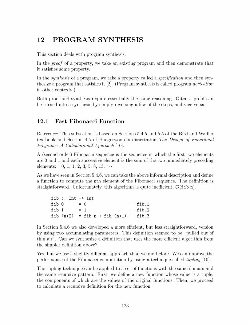
12 PROGRAM SYNTHESIS

This section deals with program synthesis.

In the proof of a property, we take an existing program and then demonstrate thatit satisfies some property.

In the synthesis of a program, we take a property called a specification and then syn-thesize a program that satisfies it [2]. (Program synthesis is called program derivationin other contexts.)

Both proof and synthesis require essentially the same reasoning. Often a proof canbe turned into a synthesis by simply reversing a few of the steps, and vice versa.

12.1 Fast Fibonacci Function

Reference: This subsection is based on Sections 5.4.5 and 5.5 of the Bird and Wadlertextbook and Section 4.5 of Hoogerwoord’s dissertation The Design of FunctionalPrograms: A Calculational Approach [10].

A (second-order) Fibonacci sequence is the sequence in which the first two elementsare 0 and 1 and each successive element is the sum of the two immediately precedingelements: 0, 1, 1, 2, 3, 5, 8, 13, · · ·

As we have seen in Section 5.4.6, we can take the above informal description and definea function to compute the nth element of the Fibonacci sequence. The definition isstraightforward. Unfortunately, this algorithm is quite inefficient, O(fib n).

fib :: Int -> Int

fib 0 = 0 -- fib.1

fib 1 = 1 -- fib.2

fib (n+2) = fib n + fib (n+1) -- fib.3

In Section 5.4.6 we also developed a more efficient, but less straightforward, versionby using two accumulating parameters. This definition seemed to be “pulled out ofthin air”. Can we synthesize a definition that uses the more efficient algorithm fromthe simpler definition above?

Yes, but we use a slightly different approach than we did before. We can improve theperformance of the Fibonacci computation by using a technique called tupling [10].

The tupling technique can be applied to a set of functions with the same domain andthe same recursive pattern. First, we define a new function whose value is a tuple,the components of which are the values of the original functions. Then, we proceedto calculate a recursive definition for the new function.

123

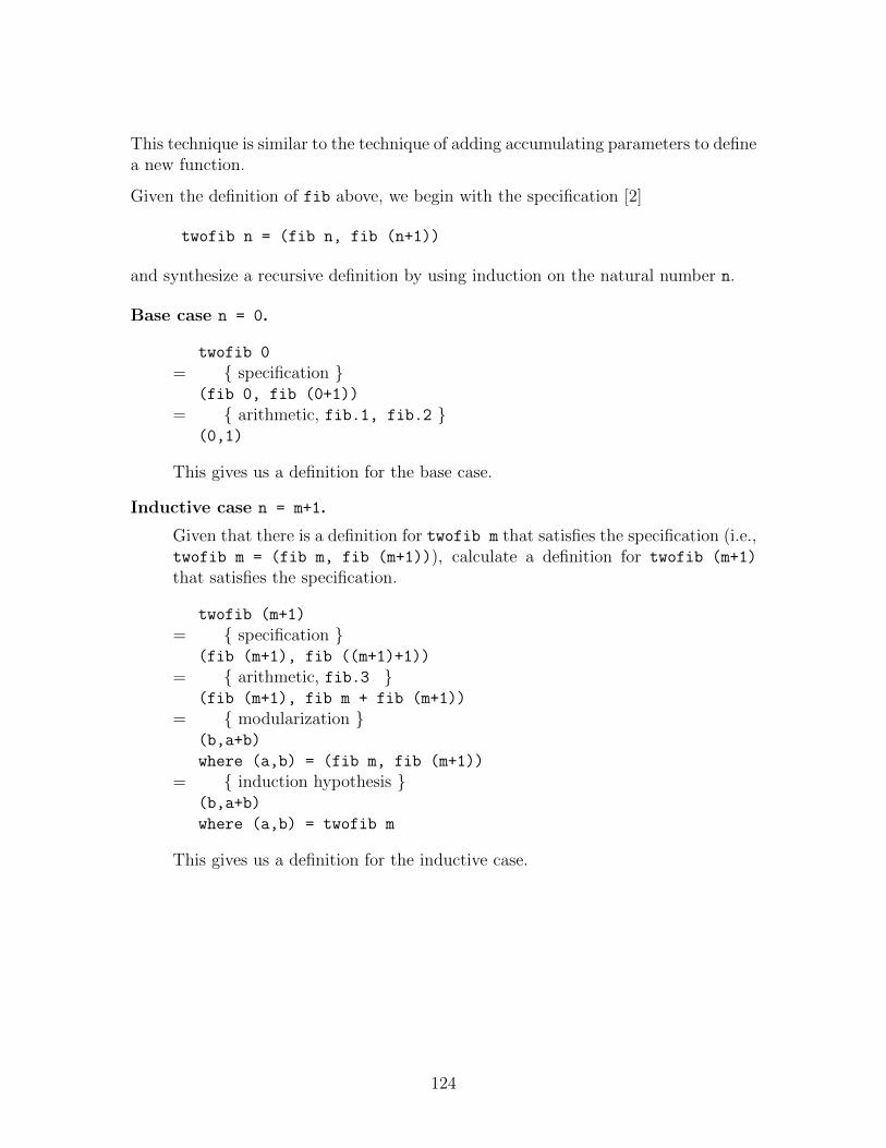
This technique is similar to the technique of adding accumulating parameters to definea new function.

Given the definition of fib above, we begin with the specification [2]

twofib n = (fib n, fib (n+1))

and synthesize a recursive definition by using induction on the natural number n.

Base case n = 0.

twofib 0

= { specification }(fib 0, fib (0+1))

= { arithmetic, fib.1, fib.2 }(0,1)

This gives us a definition for the base case.

Inductive case n = m+1.

Given that there is a definition for twofib m that satisfies the specification (i.e.,twofib m = (fib m, fib (m+1))), calculate a definition for twofib (m+1)

that satisfies the specification.

twofib (m+1)

= { specification }(fib (m+1), fib ((m+1)+1))

= { arithmetic, fib.3 }(fib (m+1), fib m + fib (m+1))

= { modularization }(b,a+b)

where (a,b) = (fib m, fib (m+1))

= { induction hypothesis }(b,a+b)

where (a,b) = twofib m

This gives us a definition for the inductive case.

124

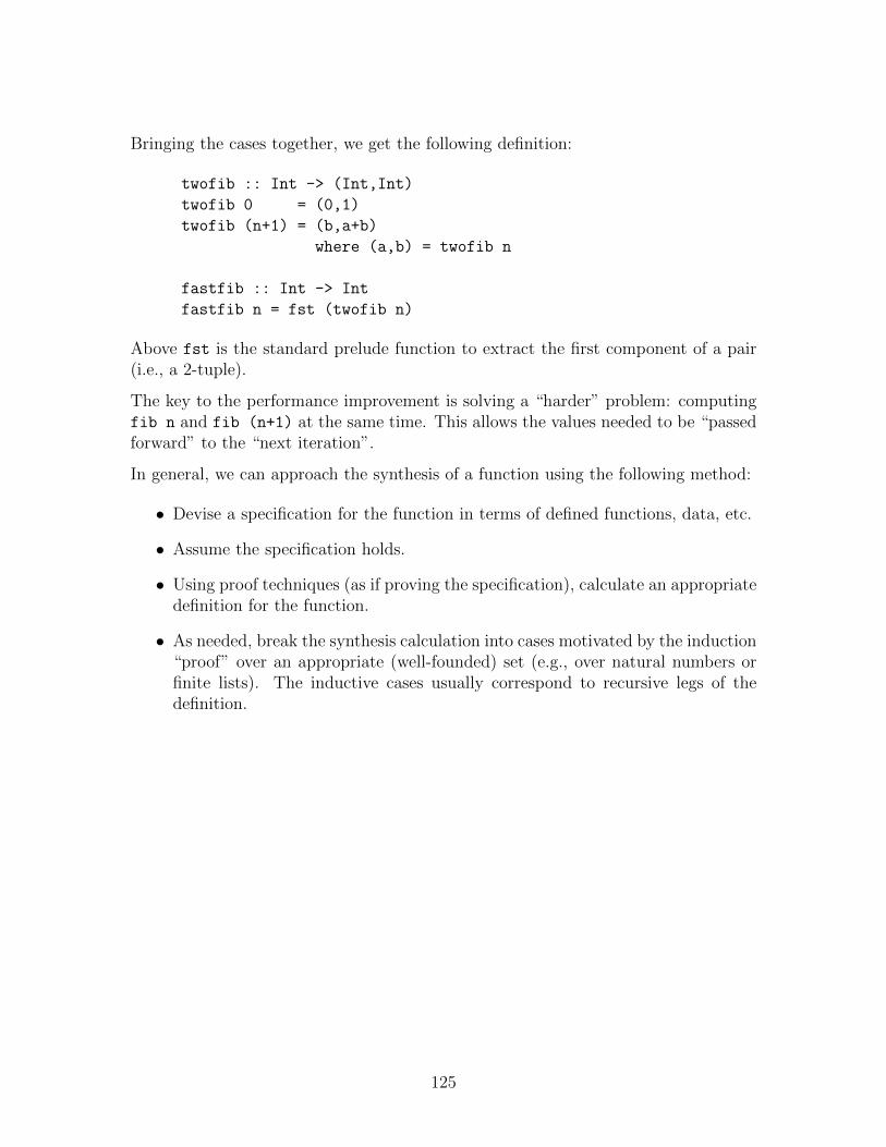
Bringing the cases together, we get the following definition:

twofib :: Int -> (Int,Int)

twofib 0 = (0,1)

twofib (n+1) = (b,a+b)

where (a,b) = twofib n

fastfib :: Int -> Int

fastfib n = fst (twofib n)

Above fst is the standard prelude function to extract the first component of a pair(i.e., a 2-tuple).

The key to the performance improvement is solving a “harder” problem: computingfib n and fib (n+1) at the same time. This allows the values needed to be “passedforward” to the “next iteration”.

In general, we can approach the synthesis of a function using the following method:

• Devise a specification for the function in terms of defined functions, data, etc.

• Assume the specification holds.

• Using proof techniques (as if proving the specification), calculate an appropriatedefinition for the function.

• As needed, break the synthesis calculation into cases motivated by the induction“proof” over an appropriate (well-founded) set (e.g., over natural numbers orfinite lists). The inductive cases usually correspond to recursive legs of thedefinition.

125

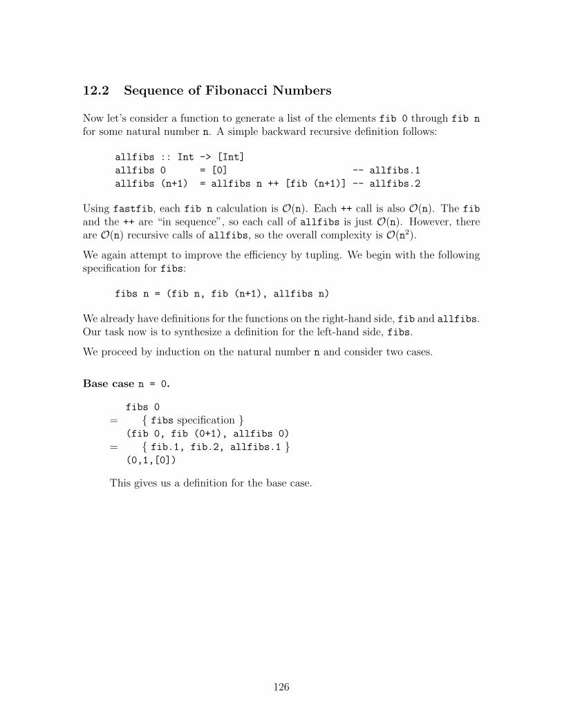
12.2 Sequence of Fibonacci Numbers

Now let’s consider a function to generate a list of the elements fib 0 through fib n

for some natural number n. A simple backward recursive definition follows:

allfibs :: Int -> [Int]

allfibs 0 = [0] -- allfibs.1

allfibs (n+1) = allfibs n ++ [fib (n+1)] -- allfibs.2

Using fastfib, each fib n calculation is O(n). Each ++ call is also O(n). The fib

and the ++ are “in sequence”, so each call of allfibs is just O(n). However, thereare O(n) recursive calls of allfibs, so the overall complexity is O(n2).

We again attempt to improve the efficiency by tupling. We begin with the followingspecification for fibs:

fibs n = (fib n, fib (n+1), allfibs n)

We already have definitions for the functions on the right-hand side, fib and allfibs.Our task now is to synthesize a definition for the left-hand side, fibs.

We proceed by induction on the natural number n and consider two cases.

Base case n = 0.

fibs 0

= { fibs specification }(fib 0, fib (0+1), allfibs 0)

= { fib.1, fib.2, allfibs.1 }(0,1,[0])

This gives us a definition for the base case.

126

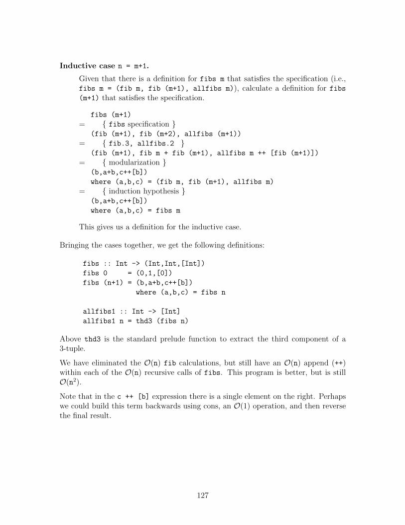
Inductive case n = m+1.

Given that there is a definition for fibs m that satisfies the specification (i.e.,fibs m = (fib m, fib (m+1), allfibs m)), calculate a definition for fibs

(m+1) that satisfies the specification.

fibs (m+1)

= { fibs specification }(fib (m+1), fib (m+2), allfibs (m+1))

= { fib.3, allfibs.2 }(fib (m+1), fib m + fib (m+1), allfibs m ++ [fib (m+1)])

= { modularization }(b,a+b,c++[b])

where (a,b,c) = (fib m, fib (m+1), allfibs m)

= { induction hypothesis }(b,a+b,c++[b])

where (a,b,c) = fibs m

This gives us a definition for the inductive case.

Bringing the cases together, we get the following definitions:

fibs :: Int -> (Int,Int,[Int])

fibs 0 = (0,1,[0])

fibs (n+1) = (b,a+b,c++[b])

where (a,b,c) = fibs n

allfibs1 :: Int -> [Int]

allfibs1 n = thd3 (fibs n)

Above thd3 is the standard prelude function to extract the third component of a3-tuple.

We have eliminated the O(n) fib calculations, but still have an O(n) append (++)within each of the O(n) recursive calls of fibs. This program is better, but is stillO(n2).

Note that in the c ++ [b] expression there is a single element on the right. Perhapswe could build this term backwards using cons, an O(1) operation, and then reversethe final result.

127

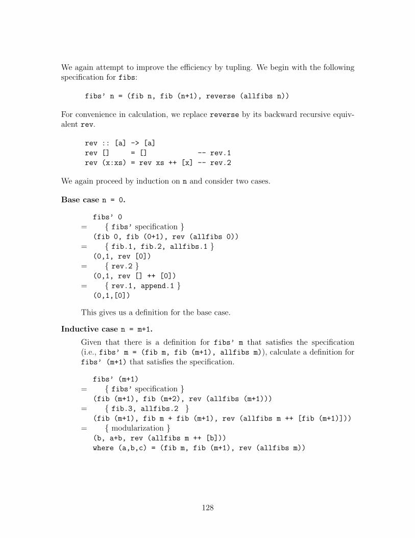
We again attempt to improve the efficiency by tupling. We begin with the followingspecification for fibs:

fibs’ n = (fib n, fib (n+1), reverse (allfibs n))

For convenience in calculation, we replace reverse by its backward recursive equiv-alent rev.

rev :: [a] -> [a]

rev [] = [] -- rev.1

rev (x:xs) = rev xs ++ [x] -- rev.2

We again proceed by induction on n and consider two cases.

Base case n = 0.

fibs’ 0

= { fibs’ specification }(fib 0, fib (0+1), rev (allfibs 0))

= { fib.1, fib.2, allfibs.1 }(0,1, rev [0])

= { rev.2 }(0,1, rev [] ++ [0])

= { rev.1, append.1 }(0,1,[0])

This gives us a definition for the base case.

Inductive case n = m+1.

Given that there is a definition for fibs’ m that satisfies the specification(i.e., fibs’ m = (fib m, fib (m+1), allfibs m)), calculate a definition forfibs’ (m+1) that satisfies the specification.

fibs’ (m+1)

= { fibs’ specification }(fib (m+1), fib (m+2), rev (allfibs (m+1)))

= { fib.3, allfibs.2 }(fib (m+1), fib m + fib (m+1), rev (allfibs m ++ [fib (m+1)]))

= { modularization }(b, a+b, rev (allfibs m ++ [b]))

where (a,b,c) = (fib m, fib (m+1), rev (allfibs m))

128

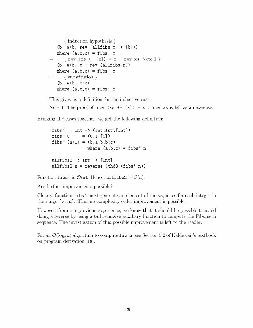
= { induction hypothesis }(b, a+b, rev (allfibs m ++ [b]))

where (a,b,c) = fibs’ m

= { rev (xs ++ [x]) = x : rev xs, Note 1 }(b, a+b, b : rev (allfibs m))

where (a,b,c) = fibs’ m

= { substitution }(b, a+b, b:c)

where (a,b,c) = fibs’ m

This gives us a definition for the inductive case.

Note 1: The proof of rev (xs ++ [x]) = x : rev xs is left as an exercise.

Bringing the cases together, we get the following definition:

fibs’ :: Int -> (Int,Int,[Int])

fibs’ 0 = (0,1,[0])

fibs’ (n+1) = (b,a+b,b:c)

where (a,b,c) = fibs’ n

allfibs2 :: Int -> [Int]

allfibs2 n = reverse (thd3 (fibs’ n))

Function fibs’ is O(n). Hence, allfibs2 is O(n).

Are further improvements possible?

Clearly, function fibs’ must generate an element of the sequence for each integer inthe range [0..n]. Thus no complexity order improvement is possible.

However, from our previous experience, we know that it should be possible to avoiddoing a reverse by using a tail recursive auxiliary function to compute the Fibonaccisequence. The investigation of this possible improvement is left to the reader.

For an O(log2 n) algorithm to compute fib n, see Section 5.2 of Kaldewaij’s textbookon program derivation [18].

129

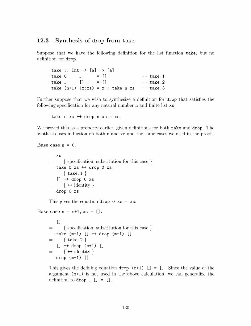
12.3 Synthesis of drop from take

Suppose that we have the following definition for the list function take, but nodefinition for drop.

take :: Int -> [a] -> [a]

take 0 = [] -- take.1

take [] = [] -- take.2

take (n+1) (x:xs) = x : take n xs -- take.3

Further suppose that we wish to synthesize a definition for drop that satisfies thefollowing specification for any natural number n and finite list xs.

take n xs ++ drop n xs = xs

We proved this as a property earlier, given definitions for both take and drop. Thesynthesis uses induction on both n and xs and the same cases we used in the proof.

Base case n = 0.

xs

= { specification, substitution for this case }take 0 xs ++ drop 0 xs

= { take.1 }[] ++ drop 0 xs

= { ++ identity }drop 0 xs

This gives the equation drop 0 xs = xs.

Base case n = m+1, xs = [].

[]

= { specification, substitution for this case }take (m+1) [] ++ drop (m+1) []

= { take.2 }[] ++ drop (m+1) []

= { ++ identity }drop (m+1) []

This gives the defining equation drop (m+1) [] = []. Since the value of theargument (m+1) is not used in the above calculation, we can generalize thedefinition to drop [] = [].

130

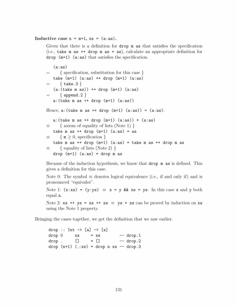
Inductive case n = m+1, xs = (a:as).

Given that there is a definition for drop m as that satisfies the specification(i.e., take m as ++ drop m as = as), calculate an appropriate definition fordrop (m+1) (a:as) that satisfies the specification.

(a:as)

= { specification, substitution for this case }take (m+1) (a:as) ++ drop (m+1) (a:as)

= { take.3 }(a:(take m as)) ++ drop (m+1) (a:as)

= { append.2 }a:(take m as ++ drop (m+1) (a:as))

Hence, a:(take m as ++ drop (m+1) (a:as)) = (a:as).

a:(take m as ++ drop (m+1) (a:as)) = (a:as)

≡ { axiom of equality of lists (Note 1) }take m as ++ drop (m+1) (a:as) = as

≡ { m ≥ 0, specification }take m as ++ drop (m+1) (a:as) = take m as ++ drop m as

≡ { equality of lists (Note 2) }drop (m+1) (a:as) = drop m as

Because of the induction hypothesis, we know that drop m as is defined. Thisgives a definition for this case.

Note 0: The symbol ≡ denotes logical equivalence (i.e., if and only if) and ispronounced “equivales”.

Note 1: (x:xs) = (y:ys) ≡ x = y && xs = ys. In this case x and y bothequal a.

Note 2: xs ++ ys = xs ++ zs ≡ ys = zs can be proved by induction on xs

using the Note 1 property.

Bringing the cases together, we get the definition that we saw earlier.

drop :: Int -> [a] -> [a]

drop 0 xs = xs -- drop.1

drop [] = [] -- drop.2

drop (n+1) ( :xs) = drop n xs -- drop.3

131

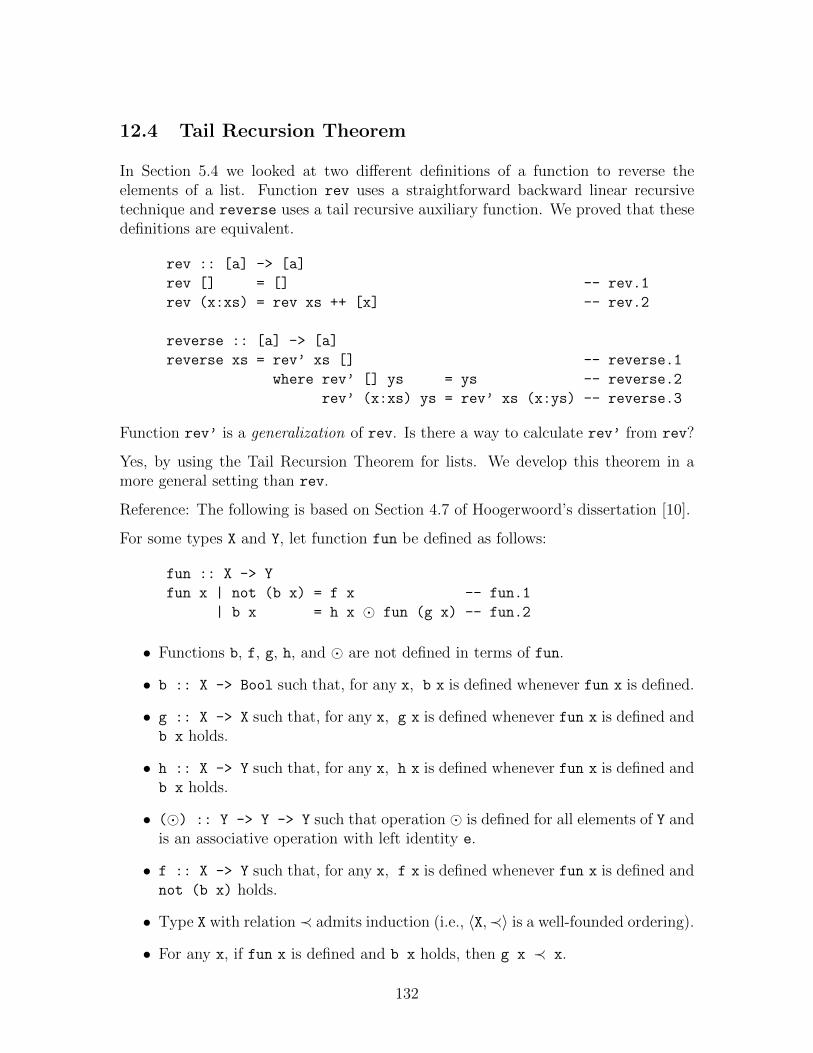
12.4 Tail Recursion Theorem

In Section 5.4 we looked at two different definitions of a function to reverse theelements of a list. Function rev uses a straightforward backward linear recursivetechnique and reverse uses a tail recursive auxiliary function. We proved that thesedefinitions are equivalent.

rev :: [a] -> [a]

rev [] = [] -- rev.1

rev (x:xs) = rev xs ++ [x] -- rev.2

reverse :: [a] -> [a]

reverse xs = rev’ xs [] -- reverse.1

where rev’ [] ys = ys -- reverse.2

rev’ (x:xs) ys = rev’ xs (x:ys) -- reverse.3

Function rev’ is a generalization of rev. Is there a way to calculate rev’ from rev?

Yes, by using the Tail Recursion Theorem for lists. We develop this theorem in amore general setting than rev.

Reference: The following is based on Section 4.7 of Hoogerwoord’s dissertation [10].

For some types X and Y, let function fun be defined as follows:

fun :: X -> Y

fun x | not (b x) = f x -- fun.1

| b x = h x � fun (g x) -- fun.2

• Functions b, f, g, h, and � are not defined in terms of fun.

• b :: X -> Bool such that, for any x, b x is defined whenever fun x is defined.

• g :: X -> X such that, for any x, g x is defined whenever fun x is defined andb x holds.

• h :: X -> Y such that, for any x, h x is defined whenever fun x is defined andb x holds.

• (�) :: Y -> Y -> Y such that operation � is defined for all elements of Y andis an associative operation with left identity e.

• f :: X -> Y such that, for any x, f x is defined whenever fun x is defined andnot (b x) holds.

• Type X with relation ≺ admits induction (i.e., 〈X,≺〉 is a well-founded ordering).

• For any x, if fun x is defined and b x holds, then g x ≺ x.

132

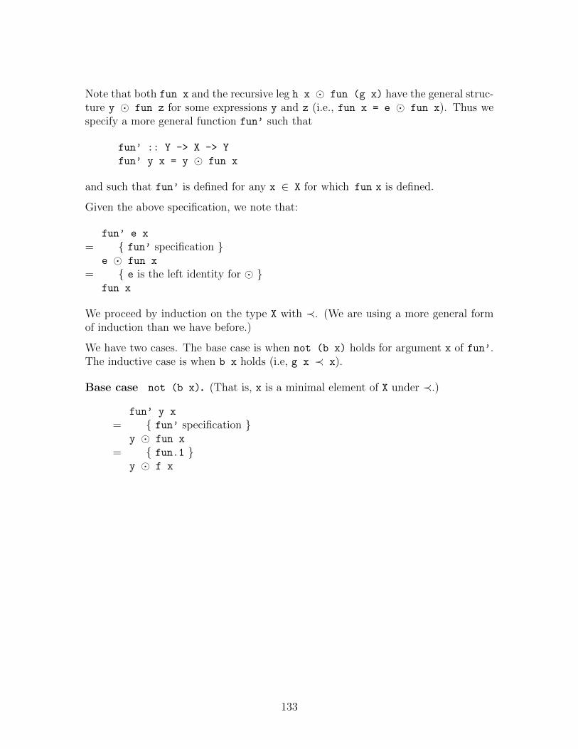
Note that both fun x and the recursive leg h x � fun (g x) have the general struc-ture y � fun z for some expressions y and z (i.e., fun x = e � fun x). Thus wespecify a more general function fun’ such that

fun’ :: Y -> X -> Y

fun’ y x = y � fun x

and such that fun’ is defined for any x ∈ X for which fun x is defined.

Given the above specification, we note that:

fun’ e x

= { fun’ specification }e � fun x

= { e is the left identity for � }fun x

We proceed by induction on the type X with ≺. (We are using a more general formof induction than we have before.)

We have two cases. The base case is when not (b x) holds for argument x of fun’.The inductive case is when b x holds (i.e, g x ≺ x).

Base case not (b x). (That is, x is a minimal element of X under ≺.)

fun’ y x

= { fun’ specification }y � fun x

= { fun.1 }y � f x

133

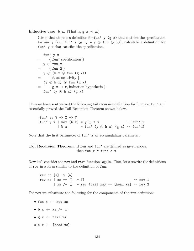
Inductive case b x. (That is, g x ≺ x.)

Given that there is a definition for fun’ y (g x) that satisfies the specificationfor any y (i.e., fun’ y (g x) = y � fun (g x)), calculate a definition forfun’ y x that satisfies the specification.

fun’ y x

= { fun’ specification }y � fun x

= { fun.2 }y � (h x � fun (g x))

= { � associativity }(y � h x) � fun (g x)

= { g x ≺ x, induction hypothesis }fun’ (y � h x) (g x)

Thus we have synthesized the following tail recursive definition for function fun’ andessentially proved the Tail Recursion Theorem shown below.

fun’ :: Y -> X -> Y

fun’ y x | not (b x) = y � f x -- fun’.1

| b x = fun’ (y � h x) (g x) -- fun’.2

Note that the first parameter of fun’ is an accumulating parameter.

Tail Recursion Theorem: If fun and fun’ are defined as given above,then fun x = fun’ e x.

Now let’s consider the rev and rev’ functions again. First, let’s rewrite the definitionsof rev in a form similar to the definition of fun.

rev :: [a] -> [a]

rev xs | xs == [] = [] -- rev.1

| xs /= [] = rev (tail xs) ++ [head xs] -- rev.2

For rev we substitute the following for the components of the fun definition:

• fun x ← rev xs

• b x ← xs /= []

• g x ← tail xs

• h x ← [head xs]

134

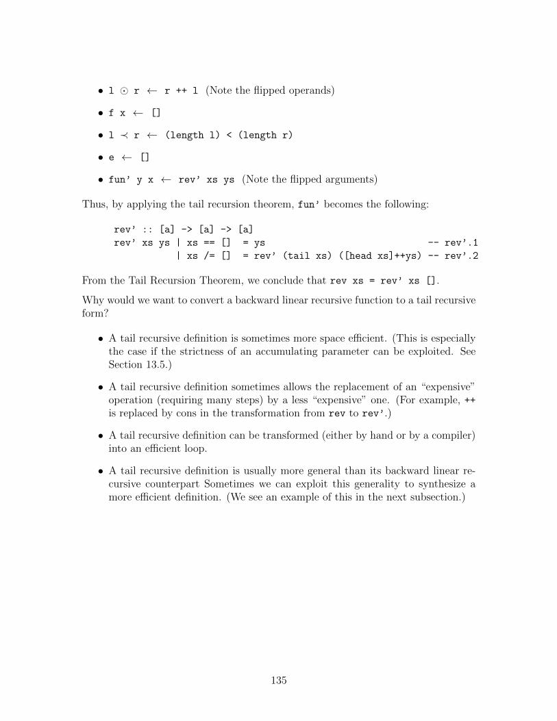
• l � r ← r ++ l (Note the flipped operands)

• f x ← []

• l ≺ r ← (length l) < (length r)

• e ← []

• fun’ y x ← rev’ xs ys (Note the flipped arguments)

Thus, by applying the tail recursion theorem, fun’ becomes the following:

rev’ :: [a] -> [a] -> [a]

rev’ xs ys | xs == [] = ys -- rev’.1

| xs /= [] = rev’ (tail xs) ([head xs]++ys) -- rev’.2

From the Tail Recursion Theorem, we conclude that rev xs = rev’ xs [].

Why would we want to convert a backward linear recursive function to a tail recursiveform?

• A tail recursive definition is sometimes more space efficient. (This is especiallythe case if the strictness of an accumulating parameter can be exploited. SeeSection 13.5.)

• A tail recursive definition sometimes allows the replacement of an “expensive”operation (requiring many steps) by a less “expensive” one. (For example, ++is replaced by cons in the transformation from rev to rev’.)

• A tail recursive definition can be transformed (either by hand or by a compiler)into an efficient loop.

• A tail recursive definition is usually more general than its backward linear re-cursive counterpart Sometimes we can exploit this generality to synthesize amore efficient definition. (We see an example of this in the next subsection.)

135

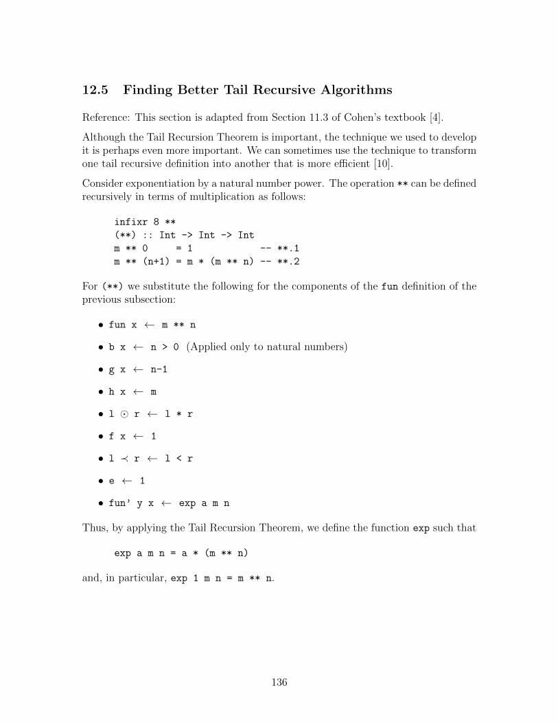
12.5 Finding Better Tail Recursive Algorithms

Reference: This section is adapted from Section 11.3 of Cohen’s textbook [4].

Although the Tail Recursion Theorem is important, the technique we used to developit is perhaps even more important. We can sometimes use the technique to transformone tail recursive definition into another that is more efficient [10].

Consider exponentiation by a natural number power. The operation ** can be definedrecursively in terms of multiplication as follows:

infixr 8 **

(**) :: Int -> Int -> Int

m ** 0 = 1 -- **.1

m ** (n+1) = m * (m ** n) -- **.2

For (**) we substitute the following for the components of the fun definition of theprevious subsection:

• fun x ← m ** n

• b x ← n > 0 (Applied only to natural numbers)

• g x ← n-1

• h x ← m

• l � r ← l * r

• f x ← 1

• l ≺ r ← l < r

• e ← 1

• fun’ y x ← exp a m n

Thus, by applying the Tail Recursion Theorem, we define the function exp such that

exp a m n = a * (m ** n)

and, in particular, exp 1 m n = m ** n.

136

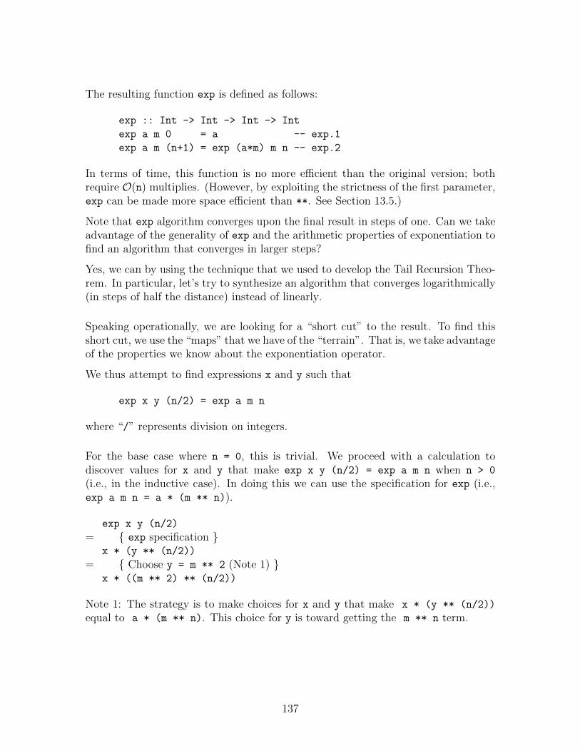
The resulting function exp is defined as follows:

exp :: Int -> Int -> Int -> Int

exp a m 0 = a -- exp.1

exp a m (n+1) = exp (a*m) m n -- exp.2

In terms of time, this function is no more efficient than the original version; bothrequire O(n) multiplies. (However, by exploiting the strictness of the first parameter,exp can be made more space efficient than **. See Section 13.5.)

Note that exp algorithm converges upon the final result in steps of one. Can we takeadvantage of the generality of exp and the arithmetic properties of exponentiation tofind an algorithm that converges in larger steps?

Yes, we can by using the technique that we used to develop the Tail Recursion Theo-rem. In particular, let’s try to synthesize an algorithm that converges logarithmically(in steps of half the distance) instead of linearly.

Speaking operationally, we are looking for a “short cut” to the result. To find thisshort cut, we use the “maps” that we have of the “terrain”. That is, we take advantageof the properties we know about the exponentiation operator.

We thus attempt to find expressions x and y such that

exp x y (n/2) = exp a m n

where “/” represents division on integers.

For the base case where n = 0, this is trivial. We proceed with a calculation todiscover values for x and y that make exp x y (n/2) = exp a m n when n > 0

(i.e., in the inductive case). In doing this we can use the specification for exp (i.e.,exp a m n = a * (m ** n)).

exp x y (n/2)

= { exp specification }x * (y ** (n/2))

= { Choose y = m ** 2 (Note 1) }x * ((m ** 2) ** (n/2))

Note 1: The strategy is to make choices for x and y that make x * (y ** (n/2))

equal to a * (m ** n). This choice for y is toward getting the m ** n term.

137

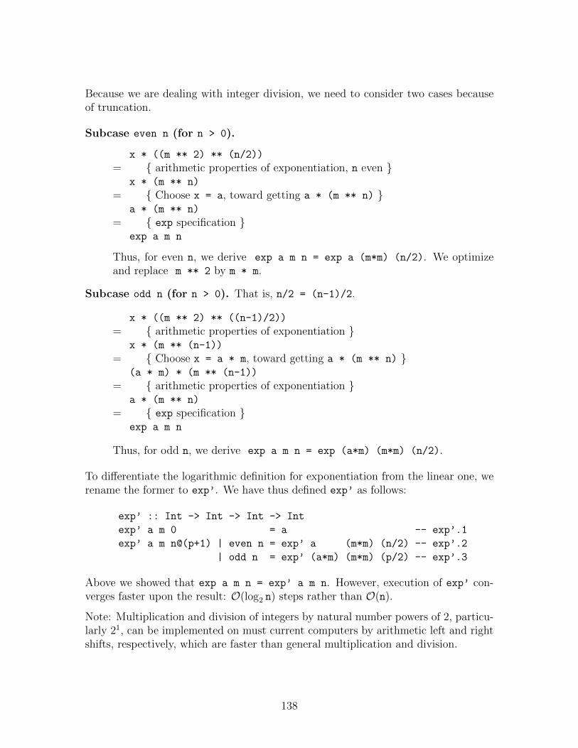
Because we are dealing with integer division, we need to consider two cases becauseof truncation.

Subcase even n (for n > 0).

x * ((m ** 2) ** (n/2))

= { arithmetic properties of exponentiation, n even }x * (m ** n)

= { Choose x = a, toward getting a * (m ** n) }a * (m ** n)

= { exp specification }exp a m n

Thus, for even n, we derive exp a m n = exp a (m*m) (n/2). We optimizeand replace m ** 2 by m * m.

Subcase odd n (for n > 0). That is, n/2 = (n-1)/2.

x * ((m ** 2) ** ((n-1)/2))

= { arithmetic properties of exponentiation }x * (m ** (n-1))

= { Choose x = a * m, toward getting a * (m ** n) }(a * m) * (m ** (n-1))

= { arithmetic properties of exponentiation }a * (m ** n)

= { exp specification }exp a m n

Thus, for odd n, we derive exp a m n = exp (a*m) (m*m) (n/2).

To differentiate the logarithmic definition for exponentiation from the linear one, werename the former to exp’. We have thus defined exp’ as follows:

exp’ :: Int -> Int -> Int -> Int

exp’ a m 0 = a -- exp’.1

exp’ a m n@(p+1) | even n = exp’ a (m*m) (n/2) -- exp’.2

| odd n = exp’ (a*m) (m*m) (p/2) -- exp’.3

Above we showed that exp a m n = exp’ a m n. However, execution of exp’ con-verges faster upon the result: O(log2 n) steps rather than O(n).

Note: Multiplication and division of integers by natural number powers of 2, particu-larly 21, can be implemented on must current computers by arithmetic left and rightshifts, respectively, which are faster than general multiplication and division.

138

12.6 Text Processing Example

Reference: In this section we develop a text processing package similar to the one inSection 4.3 of the Bird and Wadler textbook [2]. The text processing package in theHaskell standard prelude is slightly different in its treatment of newline characters.

A textual document can be viewed in many different ways. At the lowest level, wecan view it as just a character string and define a type synonym as follows:

type Text = String

However, for other purposes, we may want to consider the document as having morestructure, i.e., view it as a sequence of words, lines, paragraphs, pages, etc. Wesometimes want to convert the text from one view to another.

12.6.1 Line processing

Consider the problem of converting a Text document to the corresponding sequenceof lines. Suppose that in the Text document, the newline characters (’\n’) serve asseparators of lines, not themselves part of the lines. Since each line is a sequence ofcharacters, we define a type synonym Line as follows:

type Line = String

We want a function lines’ that will take a Text document and return the corre-sponding sequence of lines in the document. The function has the type signature:

lines’ :: Text -> [Line]

Example: lines’ "This has\nthree \nlines"

=⇒ ["This has", "three ", "lines"]

Writing function lines’ is not trivial. However, its inverse unlines’ is quite easy.Function unlines’ takes a list of Lines, inserts a newline character between each pairof adjacent lines, and returns the Text document resulting from the concatenation.

unlines’ :: [Line] -> Text

Let’s see if we can develop lines’ from unlines’.

The basic computational pattern for function unlines’ is a folding operation. Sincewe are dealing with the construction of a list and the list constructors are nonstrictin their right arguments, a foldr operation seems more appropriate than a foldl

operation. (See Section 13.6.)

139

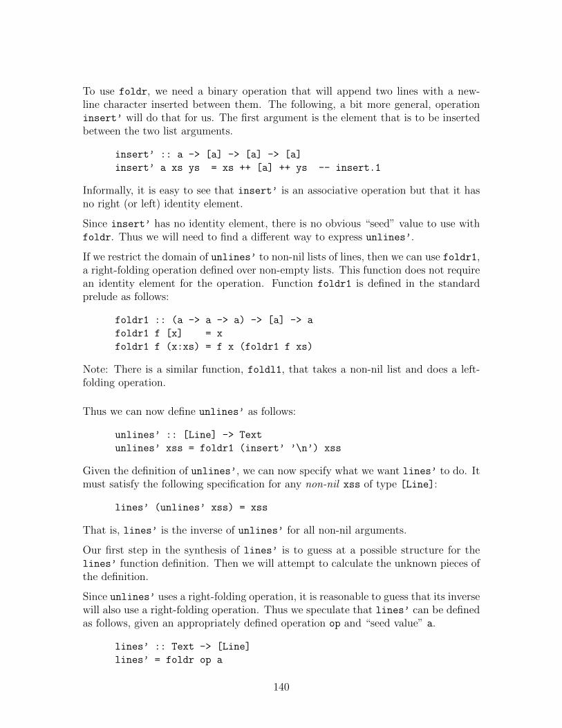
To use foldr, we need a binary operation that will append two lines with a new-line character inserted between them. The following, a bit more general, operationinsert’ will do that for us. The first argument is the element that is to be insertedbetween the two list arguments.

insert’ :: a -> [a] -> [a] -> [a]

insert’ a xs ys = xs ++ [a] ++ ys -- insert.1

Informally, it is easy to see that insert’ is an associative operation but that it hasno right (or left) identity element.

Since insert’ has no identity element, there is no obvious “seed” value to use withfoldr. Thus we will need to find a different way to express unlines’.

If we restrict the domain of unlines’ to non-nil lists of lines, then we can use foldr1,a right-folding operation defined over non-empty lists. This function does not requirean identity element for the operation. Function foldr1 is defined in the standardprelude as follows:

foldr1 :: (a -> a -> a) -> [a] -> a

foldr1 f [x] = x

foldr1 f (x:xs) = f x (foldr1 f xs)

Note: There is a similar function, foldl1, that takes a non-nil list and does a left-folding operation.

Thus we can now define unlines’ as follows:

unlines’ :: [Line] -> Text

unlines’ xss = foldr1 (insert’ ’\n’) xss

Given the definition of unlines’, we can now specify what we want lines’ to do. Itmust satisfy the following specification for any non-nil xss of type [Line]:

lines’ (unlines’ xss) = xss

That is, lines’ is the inverse of unlines’ for all non-nil arguments.

Our first step in the synthesis of lines’ is to guess at a possible structure for thelines’ function definition. Then we will attempt to calculate the unknown pieces ofthe definition.

Since unlines’ uses a right-folding operation, it is reasonable to guess that its inversewill also use a right-folding operation. Thus we speculate that lines’ can be definedas follows, given an appropriately defined operation op and “seed value” a.

lines’ :: Text -> [Line]

lines’ = foldr op a

140

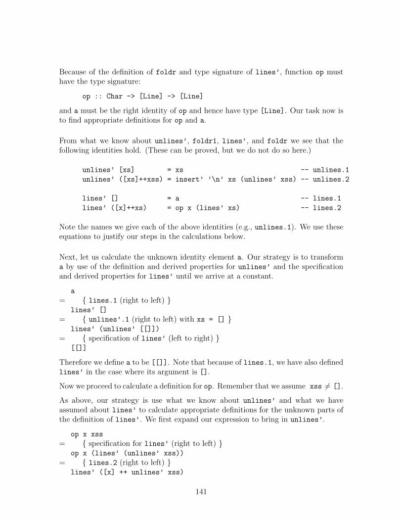
Because of the definition of foldr and type signature of lines’, function op musthave the type signature:

op :: Char -> [Line] -> [Line]

and a must be the right identity of op and hence have type [Line]. Our task now isto find appropriate definitions for op and a.

From what we know about unlines’, foldr1, lines’, and foldr we see that thefollowing identities hold. (These can be proved, but we do not do so here.)

unlines’ [xs] = xs -- unlines.1

unlines’ ([xs]++xss) = insert’ ’\n’ xs (unlines’ xss) -- unlines.2

lines’ [] = a -- lines.1

lines’ ([x]++xs) = op x (lines’ xs) -- lines.2

Note the names we give each of the above identities (e.g., unlines.1). We use theseequations to justify our steps in the calculations below.

Next, let us calculate the unknown identity element a. Our strategy is to transforma by use of the definition and derived properties for unlines’ and the specificationand derived properties for lines’ until we arrive at a constant.

a

= { lines.1 (right to left) }lines’ []

= { unlines’.1 (right to left) with xs = [] }lines’ (unlines’ [[]])

= { specification of lines’ (left to right) }[[]]

Therefore we define a to be [[]]. Note that because of lines.1, we have also definedlines’ in the case where its argument is [].

Now we proceed to calculate a definition for op. Remember that we assume xss 6= [].

As above, our strategy is use what we know about unlines’ and what we haveassumed about lines’ to calculate appropriate definitions for the unknown parts ofthe definition of lines’. We first expand our expression to bring in unlines’.

op x xss

= { specification for lines’ (right to left) }op x (lines’ (unlines’ xss))

= { lines.2 (right to left) }lines’ ([x] ++ unlines’ xss)

141

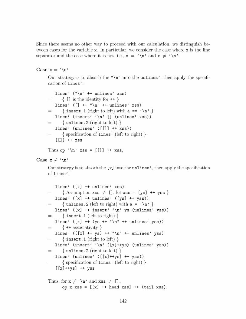
Since there seems no other way to proceed with our calculation, we distinguish be-tween cases for the variable x. In particular, we consider the case where x is the lineseparator and the case where it is not, i.e., x = ’\n’ and x 6= ’\n’.

Case x = ’\n’

Our strategy is to absorb the "\n" into the unlines’, then apply the specifi-cation of lines’.

lines’ ("\n" ++ unlines’ xss)

= { [] is the identity for ++ }lines’ ([] ++ "\n" ++ unlines’ xss)

= { insert.1 (right to left) with a == ’\n’ }lines’ (insert’ ’\n’ [] (unlines’ xss))

= { unlines.2 (right to left) }lines’ (unlines’ ([[]] ++ xss))

= { specification of lines’ (left to right) }[[]] ++ xss

Thus op ’\n’ xss = [[]] ++ xss,

Case x 6= ’\n’

Our strategy is to absorb the [x] into the unlines’, then apply the specificationof lines’.

lines’ ([x] ++ unlines’ xss)

= { Assumption xss 6= [], let xss = [ys] ++ yss }lines’ ([x] ++ unlines’ ([ys] ++ yss))

= { unlines.2 (left to right) with a = ’\n’ }lines’ ([x] ++ insert’ ’\n’ ys (unlines’ yss))

= { insert.1 (left to right) }lines’ ([x] ++ (ys ++ "\n" ++ unlines’ yss))

= { ++ associativity }lines’ (([x] ++ ys) ++ "\n" ++ unlines’ yss)

= { insert.1 (right to left) }lines’ (insert’ ’\n’ ([x]++ys) (unlines’ yss))

= { unlines.2 (right to left) }lines’ (unlines’ ([[x]++ys] ++ yss))

= { specification of lines’ (left to right) }[[x]++ys] ++ yss

Thus, for x 6= ’\n’ and xss 6= [],op x xss = [[x] ++ head xss] ++ (tail xss).

142

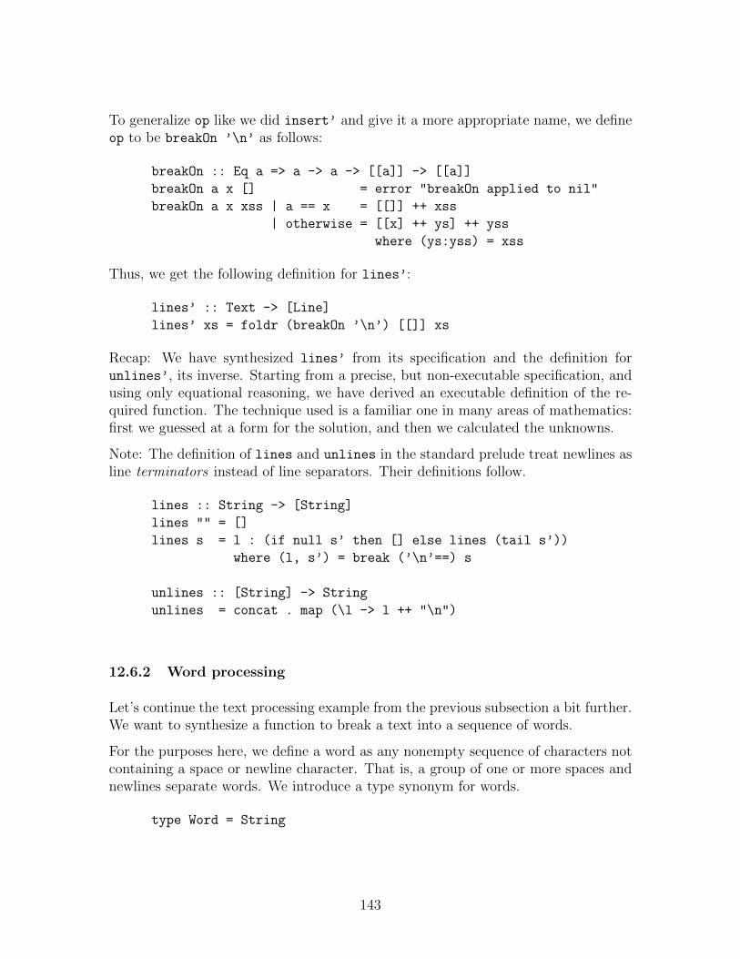
To generalize op like we did insert’ and give it a more appropriate name, we defineop to be breakOn ’\n’ as follows:

breakOn :: Eq a => a -> a -> [[a]] -> [[a]]

breakOn a x [] = error "breakOn applied to nil"

breakOn a x xss | a == x = [[]] ++ xss

| otherwise = [[x] ++ ys] ++ yss

where (ys:yss) = xss

Thus, we get the following definition for lines’:

lines’ :: Text -> [Line]

lines’ xs = foldr (breakOn ’\n’) [[]] xs

Recap: We have synthesized lines’ from its specification and the definition forunlines’, its inverse. Starting from a precise, but non-executable specification, andusing only equational reasoning, we have derived an executable definition of the re-quired function. The technique used is a familiar one in many areas of mathematics:first we guessed at a form for the solution, and then we calculated the unknowns.

Note: The definition of lines and unlines in the standard prelude treat newlines asline terminators instead of line separators. Their definitions follow.

lines :: String -> [String]

lines "" = []

lines s = l : (if null s’ then [] else lines (tail s’))

where (l, s’) = break (’\n’==) s

unlines :: [String] -> String

unlines = concat . map (\l -> l ++ "\n")

12.6.2 Word processing

Let’s continue the text processing example from the previous subsection a bit further.We want to synthesize a function to break a text into a sequence of words.

For the purposes here, we define a word as any nonempty sequence of characters notcontaining a space or newline character. That is, a group of one or more spaces andnewlines separate words. We introduce a type synonym for words.

type Word = String

143

We want a function words’ that breaks a line up into a sequence of words. Functionwords’ thus has the following type signature:

words’ :: Line -> [Word]

Example: words’ "Hi there" =⇒ ["Hi", "there"]

As in the synthesis of lines’, we proceed by defining the “inverse” function first,then we calculate the definition for words’.

All unwords’ needs to do is to insert a space character between adjacent elements ofthe sequence of words and return the concatenated result. Following the developmentin the previous subsection, we can thus define unwords’ as follows.

unwords’ :: [Word] -> Line

unwords’ xs = foldr1 (insert’ ’ ’) xs

Using calculations similar to those for lines’, we derive the inverse of unwords’ tobe the following function:

foldr (breakOn ’ ’) [[]]

However, this identifies zero-length words where there are adjacent spaces. We needto filter those out.

words’ :: Line -> [Word]

words’ = filter (/= []) . foldr (breakOn ’ ’) [[]]

Note that words’ (unwords’ xss) = xss for all xss of type [Word], but thatunwords’ (words’ xs) 6= xs for some xs of type Line. The latter is undefinedwhen words’ xs returns []. Where it is defined, adjacent spaces in xs are replacedby a single space in unwords’ (words’ xs).

Note: The functions words and unwords in the standard prelude differ in thatunwords [] = [], which is more complete.

12.6.3 Paragraph processing

Let’s continue the text processing example one step further and synthesize a functionto break a sequence of lines into paragraphs.

For the purposes here, we define a paragraph as any nonempty sequence of nonemptylines. That is, a group of one or more empty lines separate paragraphs. As above,we introduce an appropriate type synonym:

type Para = [Line]

144

We want a function paras’ that breaks a sequence of lines into a sequence of para-graphs:

paras’ :: [Line] -> [Para]

Example: paras’ ["Line 1.1","Line 1.2","","Line 2.1"]

=⇒ [["Line 1.1","Line 1.2"],["Line 2.1"]]

As in the synthesis of lines’ and words’, we can start with the inverse and calculatethe definition of paras’. The inverse function unparas’ takes a sequence of para-graphs and returns the corresponding sequence of lines with an empty line insertedbetween adjacent paragraphs.

unparas’ :: [Para] -> [Line]

unparas’ = foldr1 (insert’ [])

Using calculations similar to those for lines’ and words’, we can derive the followingdefinitions:

paras’ :: [Line] -> [Para]

paras’ = filter (/= []) . foldr (breakOn []) [[]]

The filter (/= []) operation removes all “empty paragraphs” corresponding totwo or more adjacent empty lines.

Note: There are no equivalents of paras’ and unparas’ in the standard prelude. Aswith unwords, unparas’ should be redefined so that unparas’ [] = [], which ismore complete.

12.6.4 Other text processing functions

Using the six functions in our text processing package, we can build other usefulfunctions.

Count the lines in a text.

countLines :: Text -> Int

countLines = length . lines’

145

Count the words in a text.

countWords :: Text -> Int

countWords = length . concat . (map words’) . lines’

An alternative using a list comprehension is:

countWords xs = length [ w | l <- lines’ xs, w <- words’ l]

Count the paragraphs in a text.

countParas :: Text -> Int

countParas = length . paras’ . lines’

Normalize text by removing redundant empty lines and spaces.

The following functions take advantage of the fact that paras’ and words’

discard empty paragraphs and words, respectively.

normalize :: Text -> Text

normalize = unparse . parse

parse :: Text -> [[[Word]]]

parse = (map (map words’)) . paras’ . lines’

unparse :: [[[Word]]] -> Text

unparse = unlines’ . unparas’ . map (map unwords’)

We can also state parse and unparse in terms of list comprehensions.

parse xs = [ [words’ l | l <- p] | p <- paras’ (lines’ xs) ]

unparse xssss =

unlines’ (unparas’ [ [unwords’ l | l<-p] | p<-xssss])

Section 4.3.5 of the Bird and Wadler textbook goes on to build functions to fill andleft-justify lines of text.

146

12.7 Exercises

1. The following function computes the integer base 2 logarithm of a positiveinteger:

lg :: Int -> Int

lg x | x == 1 = 0

| x > 1 = 1 + lg (x/2)

Using the tail recursion theorem, write a definition for lg that is tail recursive.

2. Synthesize the recursive definition for ++ from the following specification:

xs ++ ys = foldr (:) ys xs

3. Using tupling and function fact5 from Section 3, synthesize an efficient func-tion allfacts to generate a list off factorials for natural numbers 0 throughparameter n, inclusive.

4. Consider the following recursive definition for natural number multiplication:

mul :: Int -> Int -> Int

mul m 0 = 0

mul m (n+1) = m + mul m n

This is an O(n) algorithm for computing m * n. Synthesize an alternativeoperation that is O(log2 n). Doubling (i.e., n*2) and halving (i.e, n/2 withtruncation) operations may be used but not multiplication (*) in general.

5. Derive a “more general” version of the Tail Recursion Theorem for functions ofthe shape

func :: X -> Y

func x | not (b x) = f x -- func.1

| b x = h x � func (g x) ♦ d.x -- func.2

where functions b, f, g, and h are constrained as in the definition of fun in theTail Recursion Theorem. Be sure to identify the appropriate constraints on d,�, and ♦ including the necessary properties of � and ♦.

147

148

13 MODELS OF REDUCTION

Reference: This section is based in part on Sections 6.1–6.3 of the Bird and Wadlertextbook [2] and in part on Chapter 6 of Field and Harrison’s textbook [8].

13.1 Efficiency

We state efficiency (i.e., time complexity or space complexity) of programs in termsof the “Big-O” notation and asymptotic analysis.

For example, consider the list-reversing functions rev and reverse that we havelooked at several times. We stated that the number of steps required to evaluate rev

xs is, in the worst case, “on the order of” n2 where n denotes the length of list xs.We let the number of steps be our measure of time and write

Trev(xs) = O(n2)

to mean that the time to evaluate rev xs is bounded by some (mathematical) functionthat is proportional to the square of the length of list xs.

Similarly, we write

Treverse(xs) = O(n)

to mean that the time (i.e., number of steps) to evaluate reverse xs is bounded bysome function that is proportional to the length of xs.

Note: These expressions are not really equalities. We write the more precise expres-sion, (e.g., Treverse(xs)) on the left-hand side and the less precise expression O(n) onthe right-hand side.

For short lists, the performance of rev and reverse are similar. But as the list getslong, rev requires considerably more steps than reverse.

The Big-O analysis is an asymptotic analysis. That is, it estimates the order ofmagnitude of the evaluation time as the size of the input approaches infinity (getslarge). We often do worst case analyses of time. Such analyses are usually easier todo than average-case analyses.

149

13.2 Reduction

The terms reduction, simplification, and evaluation all denote the same process:rewriting an expression in a “simpler” equivalent form. That is, they involve twokinds of replacements:

• the replacement of a subterm that satisfies the left-hand side of an equation bythe right-hand side with appropriate substitution of arguments for parameters.(This is sometimes called β-reduction.)

• the replacement of a primitive application (e.g., + or *) by its value. (This issometimes called δ-reduction.)

The term redex refers to a subterm of an expression that can be reduced.

An expression is said to be in normal form if it cannot be further reduced.

Some expressions cannot be reduced to a value. For example, 1/0 cannot be reduced;an error message is usually generated if there is an attempt to evaluate (i.e., reduce)such an expression.

For convenience, we sometimes assign the value ⊥ (pronounced “bottom”) to sucherror cases to denote that their values are undefined. Remember that this valuecannot be manipulated within a computer.

Redexes can be selected for reduction in several ways. For instance, the redex can beselected based on its position within the expression:

leftmost redex first, the leftmost reducible subterm in the expression text is re-duced before any other subterms are reduced.

rightmost redex first, the rightmost reducible subterm in the expression text isreduced before any other subterms are reduced.

The redex can also be selected based on whether or not it is contained within anotherredex:

outermost redex first, a reducible subterm that is not contained within any otherreducible subterm is reduced before one that is contained within another.

innermost redex first, a reducible subterm that contains no other reducible sub-term is reduced before one that contains others.

150

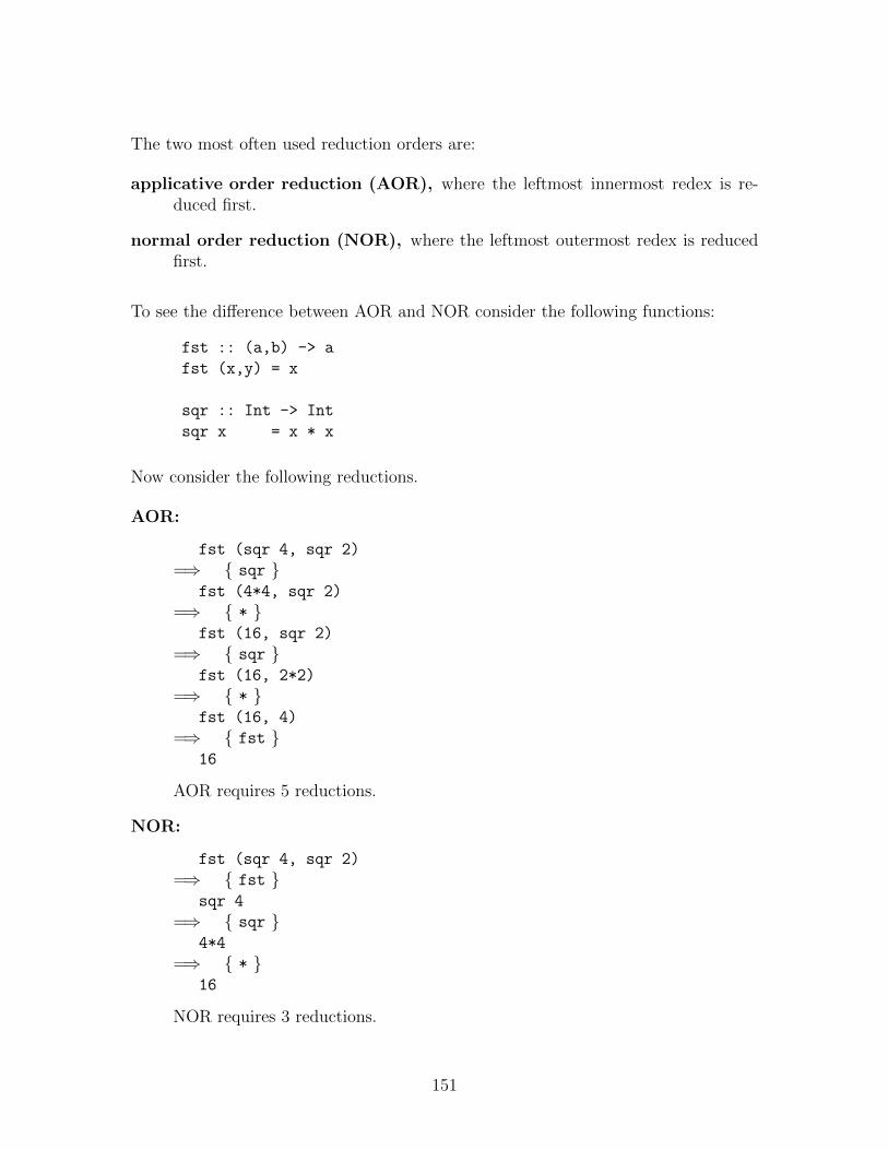
The two most often used reduction orders are:

applicative order reduction (AOR), where the leftmost innermost redex is re-duced first.

normal order reduction (NOR), where the leftmost outermost redex is reducedfirst.

To see the difference between AOR and NOR consider the following functions:

fst :: (a,b) -> a

fst (x,y) = x

sqr :: Int -> Int

sqr x = x * x

Now consider the following reductions.

AOR:

fst (sqr 4, sqr 2)

=⇒ { sqr }fst (4*4, sqr 2)

=⇒ { * }fst (16, sqr 2)

=⇒ { sqr }fst (16, 2*2)

=⇒ { * }fst (16, 4)

=⇒ { fst }16

AOR requires 5 reductions.

NOR:

fst (sqr 4, sqr 2)

=⇒ { fst }sqr 4

=⇒ { sqr }4*4

=⇒ { * }16

NOR requires 3 reductions.

151

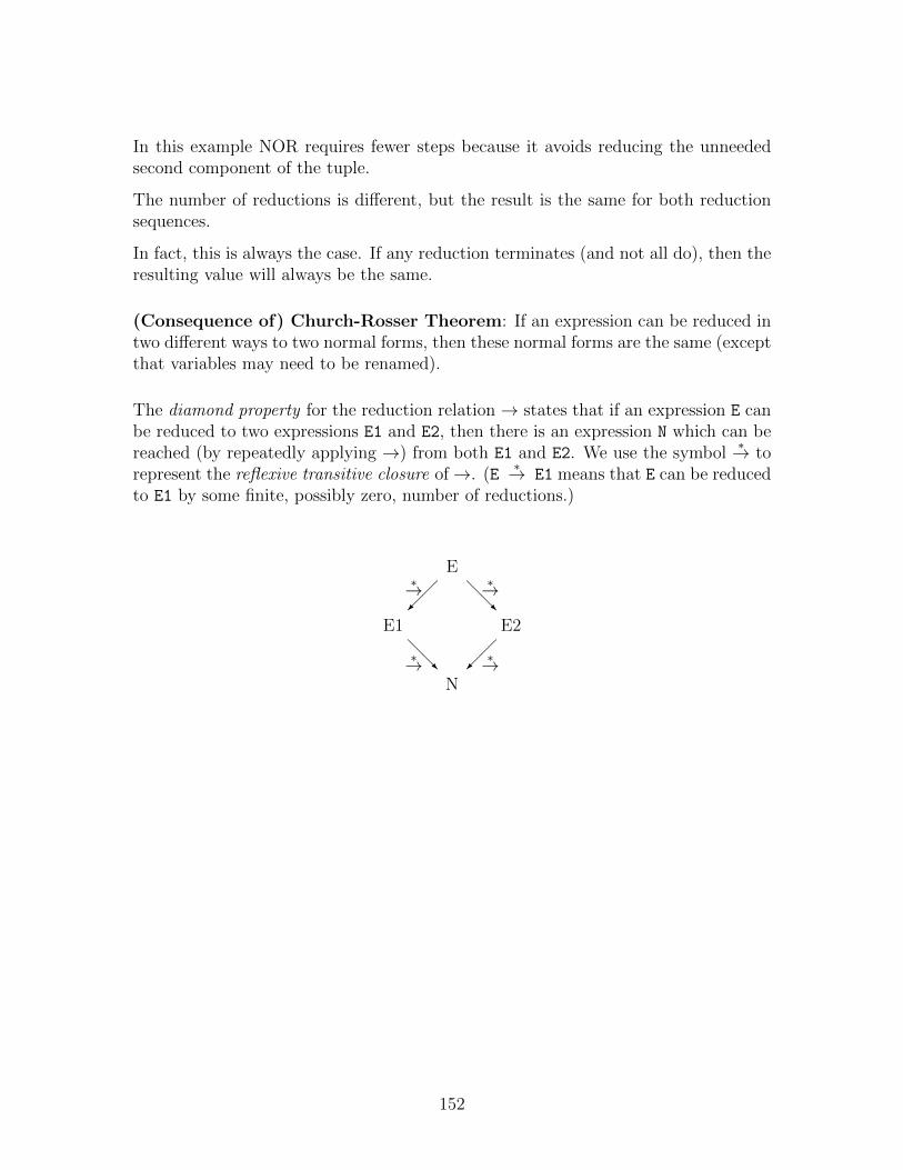
In this example NOR requires fewer steps because it avoids reducing the unneededsecond component of the tuple.

The number of reductions is different, but the result is the same for both reductionsequences.

In fact, this is always the case. If any reduction terminates (and not all do), then theresulting value will always be the same.

(Consequence of) Church-Rosser Theorem: If an expression can be reduced intwo different ways to two normal forms, then these normal forms are the same (exceptthat variables may need to be renamed).

The diamond property for the reduction relation→ states that if an expression E canbe reduced to two expressions E1 and E2, then there is an expression N which can bereached (by repeatedly applying →) from both E1 and E2. We use the symbol

∗→ torepresent the reflexive transitive closure of→. (E

∗→ E1 means that E can be reducedto E1 by some finite, possibly zero, number of reductions.)

E

��

∗→ @@R

∗→

E1 E2

@@R∗→

��∗→

N

152

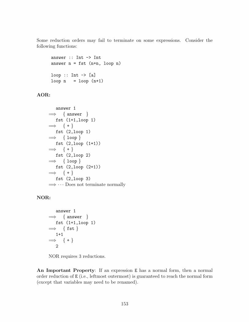
Some reduction orders may fail to terminate on some expressions. Consider thefollowing functions:

answer :: Int -> Int

answer n = fst (n+n, loop n)

loop :: Int -> [a]

loop n = loop (n+1)

AOR:

answer 1

=⇒ { answer }fst (1+1,loop 1)

=⇒ { + }fst (2,loop 1)

=⇒ { loop }fst (2,loop (1+1))

=⇒ { + }fst (2,loop 2)

=⇒ { loop }fst (2,loop (2+1))

=⇒ { + }fst (2,loop 3)

=⇒ · · · Does not terminate normally

NOR:

answer 1

=⇒ { answer }fst (1+1,loop 1)

=⇒ { fst }1+1

=⇒ { + }2

NOR requires 3 reductions.

An Important Property: If an expression E has a normal form, then a normalorder reduction of E (i.e., leftmost outermost) is guaranteed to reach the normal form(except that variables may need to be renamed).

153

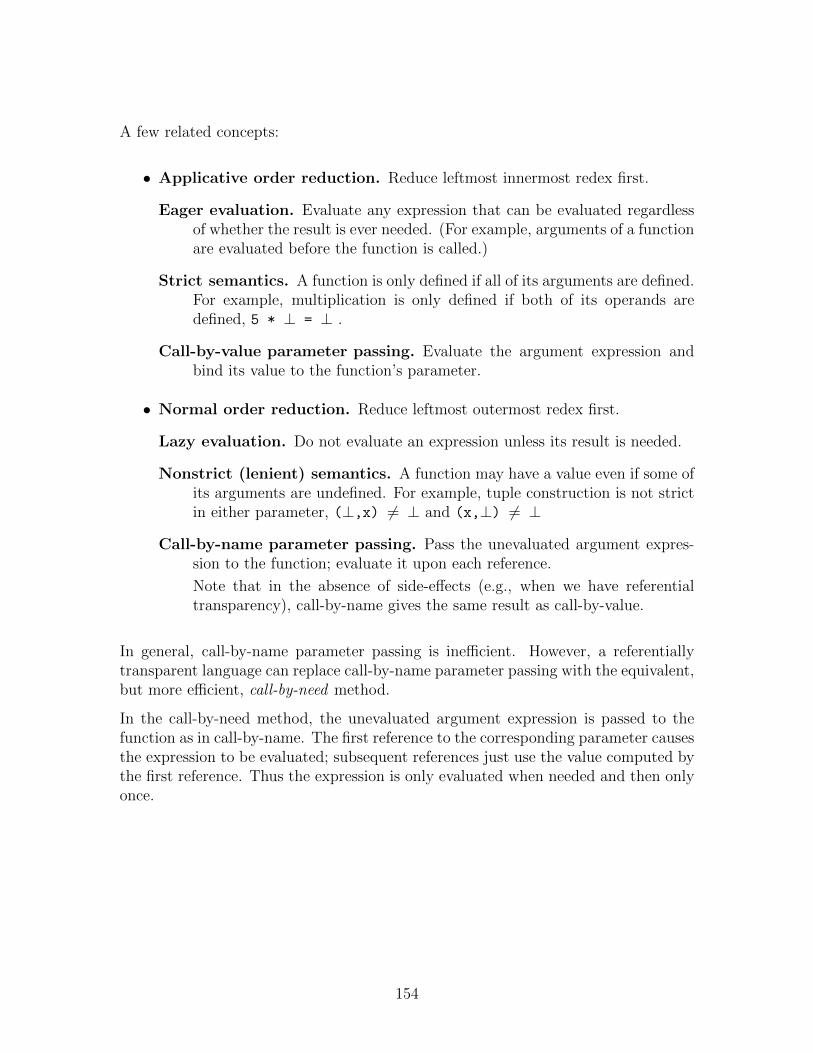
A few related concepts:

• Applicative order reduction. Reduce leftmost innermost redex first.

Eager evaluation. Evaluate any expression that can be evaluated regardlessof whether the result is ever needed. (For example, arguments of a functionare evaluated before the function is called.)

Strict semantics. A function is only defined if all of its arguments are defined.For example, multiplication is only defined if both of its operands aredefined, 5 * ⊥ = ⊥ .

Call-by-value parameter passing. Evaluate the argument expression andbind its value to the function’s parameter.

• Normal order reduction. Reduce leftmost outermost redex first.

Lazy evaluation. Do not evaluate an expression unless its result is needed.

Nonstrict (lenient) semantics. A function may have a value even if some ofits arguments are undefined. For example, tuple construction is not strictin either parameter, (⊥,x) 6= ⊥ and (x,⊥) 6= ⊥

Call-by-name parameter passing. Pass the unevaluated argument expres-sion to the function; evaluate it upon each reference.

Note that in the absence of side-effects (e.g., when we have referentialtransparency), call-by-name gives the same result as call-by-value.

In general, call-by-name parameter passing is inefficient. However, a referentiallytransparent language can replace call-by-name parameter passing with the equivalent,but more efficient, call-by-need method.

In the call-by-need method, the unevaluated argument expression is passed to thefunction as in call-by-name. The first reference to the corresponding parameter causesthe expression to be evaluated; subsequent references just use the value computed bythe first reference. Thus the expression is only evaluated when needed and then onlyonce.

154

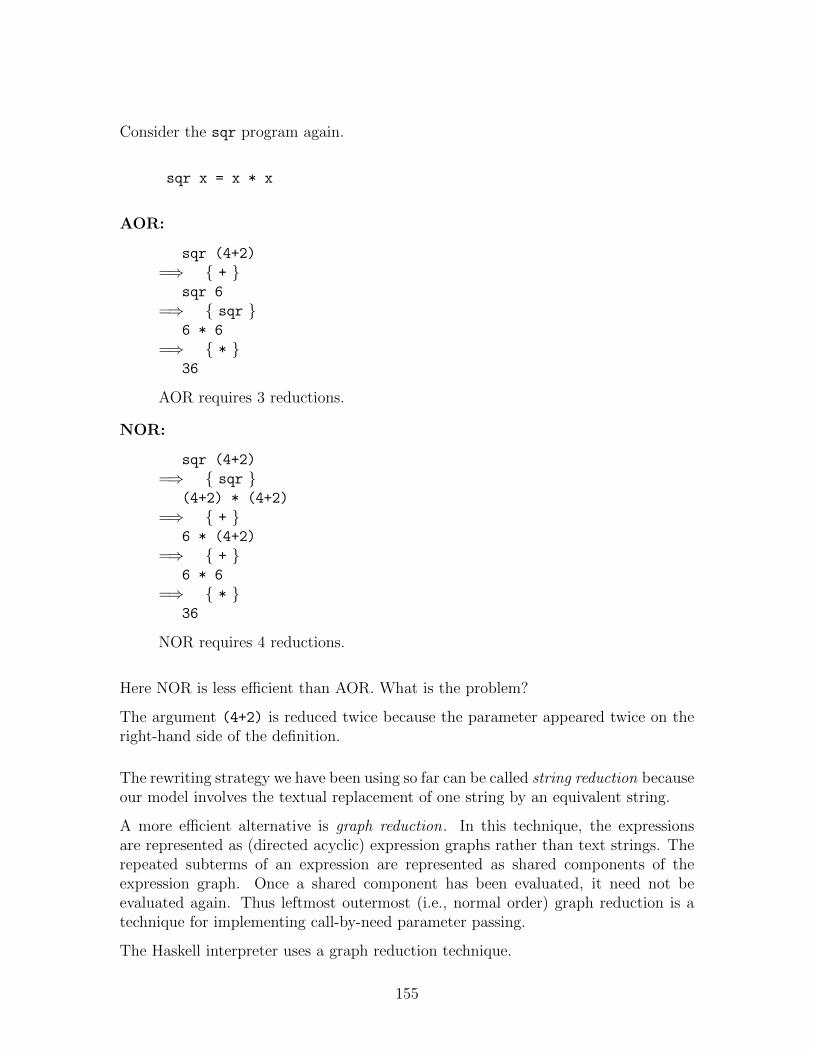
Consider the sqr program again.

sqr x = x * x

AOR:

sqr (4+2)

=⇒ { + }sqr 6

=⇒ { sqr }6 * 6

=⇒ { * }36

AOR requires 3 reductions.

NOR:

sqr (4+2)

=⇒ { sqr }(4+2) * (4+2)

=⇒ { + }6 * (4+2)

=⇒ { + }6 * 6

=⇒ { * }36

NOR requires 4 reductions.

Here NOR is less efficient than AOR. What is the problem?

The argument (4+2) is reduced twice because the parameter appeared twice on theright-hand side of the definition.

The rewriting strategy we have been using so far can be called string reduction becauseour model involves the textual replacement of one string by an equivalent string.

A more efficient alternative is graph reduction. In this technique, the expressionsare represented as (directed acyclic) expression graphs rather than text strings. Therepeated subterms of an expression are represented as shared components of theexpression graph. Once a shared component has been evaluated, it need not beevaluated again. Thus leftmost outermost (i.e., normal order) graph reduction is atechnique for implementing call-by-need parameter passing.

The Haskell interpreter uses a graph reduction technique.

155

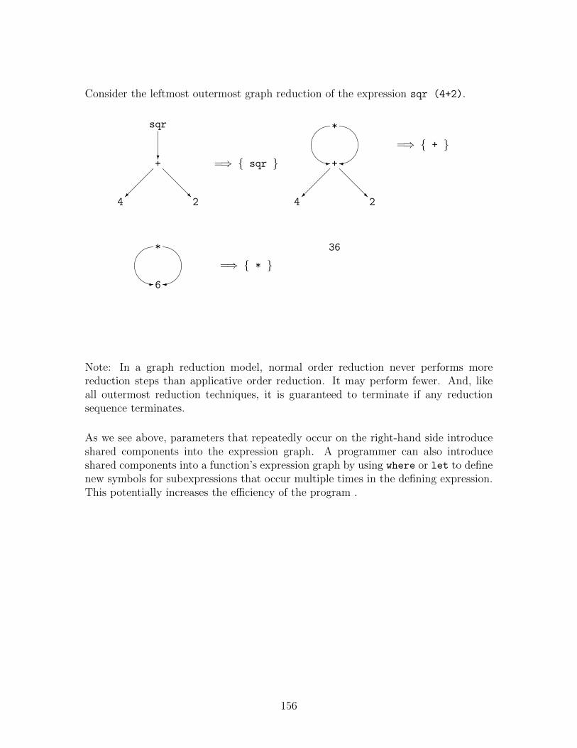
Consider the leftmost outermost graph reduction of the expression sqr (4+2).

sqr

?+

���

@@@R

4 2

=⇒ { sqr }

*'&

$%- �+

��

�

@@@R

4 2

=⇒ { + }

*'&

$%- �6

=⇒ { * }36

Note: In a graph reduction model, normal order reduction never performs morereduction steps than applicative order reduction. It may perform fewer. And, likeall outermost reduction techniques, it is guaranteed to terminate if any reductionsequence terminates.

As we see above, parameters that repeatedly occur on the right-hand side introduceshared components into the expression graph. A programmer can also introduceshared components into a function’s expression graph by using where or let to definenew symbols for subexpressions that occur multiple times in the defining expression.This potentially increases the efficiency of the program .

156

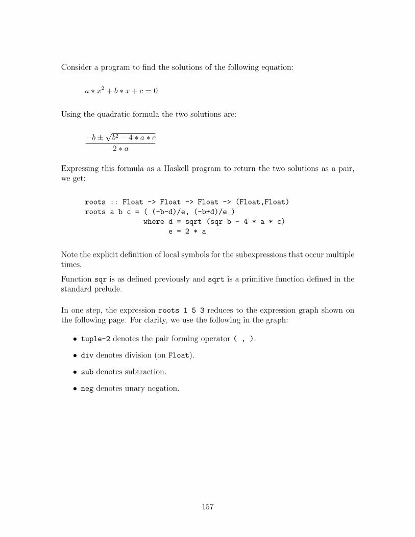
Consider a program to find the solutions of the following equation:

a ∗ x2 + b ∗ x+ c = 0

Using the quadratic formula the two solutions are:

−b±√b2 − 4 ∗ a ∗ c2 ∗ a

Expressing this formula as a Haskell program to return the two solutions as a pair,we get:

roots :: Float -> Float -> Float -> (Float,Float)

roots a b c = ( (-b-d)/e, (-b+d)/e )

where d = sqrt (sqr b - 4 * a * c)

e = 2 * a

Note the explicit definition of local symbols for the subexpressions that occur multipletimes.

Function sqr is as defined previously and sqrt is a primitive function defined in thestandard prelude.

In one step, the expression roots 1 5 3 reduces to the expression graph shown onthe following page. For clarity, we use the following in the graph:

• tuple-2 denotes the pair forming operator ( , ).

• div denotes division (on Float).

• sub denotes subtraction.

• neg denotes unary negation.

157

The application roots 1 5 3 reduces to the following expression graph:

(Drawing Not Currently Available)

158

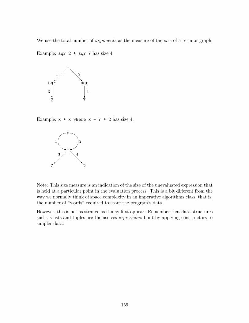
We use the total number of arguments as the measure of the size of a term or graph.

Example: sqr 2 + sqr 7 has size 4.

+�

��

1

sqr

@@@R

2

sqr

?3

2?4

7

Example: x * x where x = 7 + 2 has size 4.

*'&1

$%2- �+

���

3 @@@R

4

7 2

Note: This size measure is an indication of the size of the unevaluated expression thatis held at a particular point in the evaluation process. This is a bit different from theway we normally think of space complexity in an imperative algorithms class, that is,the number of “words” required to store the program’s data.

However, this is not as strange as it may first appear. Remember that data structuressuch as lists and tuples are themselves expressions built by applying constructors tosimpler data.

159

13.3 Head Normal Form

Sometimes we need to reduce a term but not all the way to normal form.

Consider the expression head (map sqr [1..7]) and a normal order reduction.

head (map sqr [1..7])

=⇒ { [1..7] }head (map sqr (1:[2..7]))

=⇒ { map.2 }head (sqr 1 : map sqr [2..7])

=⇒ { head }sqr 1

=⇒ { sqr }1 * 1

=⇒ { * }1

Note that the expression map sqr [1..7] was reduced but not all the way to normalform. However, any term that is reduced must be reduced to head normal form.

Definition: A term is in head normal form if:

• it is not a redex,

• it cannot become a redex by reducing any of its subterms.

If a term is in normal form, then it is in head normal form, but not vice versa.

Any term of form (e1:e2) is in head normal form, because regardless of how far e1

and e2 are reduced, no reduction rule applies to (e1:e2). The cons operator is theprimitive list constructor; it is not defined in terms of anything else.

However, a term of form (e1:e2) is only in normal form if both e1 and e2 are intheir normal forms.

Similarly, any term of the form (e1,e2) is in head normal form. The tuple constructoris a primitive operation; it is not defined in terms of anything else.

However, a term of the form (e1,e2) is in normal form only if both e1 and e2 are.

160

Whether a term needs to be reduced further than head normal form depends uponthe context.

Example: In the reduction of the expression head (map sqr [1..7]), the termmap sqr [1..7] only needed to be reduced to head normal form, that is, to theexpression sqr 1 : map sqr [2..7].

However, appendChan stdout (show (map sqr [1..7])) exit done would causereduction of map sqr [1..7] to normal form.

161

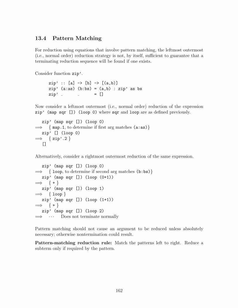
13.4 Pattern Matching

For reduction using equations that involve pattern matching, the leftmost outermost(i.e., normal order) reduction strategy is not, by itself, sufficient to guarantee that aterminating reduction sequence will be found if one exists.

Consider function zip’.

zip’ :: [a] -> [b] -> [(a,b)]

zip’ (a:as) (b:bs) = (a,b) : zip’ as bs

zip’ = []

Now consider a leftmost outermost (i.e., normal order) reduction of the expressionzip’ (map sqr []) (loop 0) where sqr and loop are as defined previously.

zip’ (map sqr []) (loop 0)

=⇒ { map.1, to determine if first arg matches (a:as)}zip’ [] (loop 0)

=⇒ { zip’.2 }[]

Alternatively, consider a rightmost outermost reduction of the same expression.

zip’ (map sqr []) (loop 0)

=⇒ { loop, to determine if second arg matches (b:bs)}zip’ (map sqr []) (loop (0+1))

=⇒ { + }zip’ (map sqr []) (loop 1)

=⇒ { loop }zip’ (map sqr []) (loop (1+1))

=⇒ { + }zip’ (map sqr []) (loop 2)

=⇒ · · · Does not terminate normally

Pattern matching should not cause an argument to be reduced unless absolutelynecessary; otherwise nontermination could result.

Pattern-matching reduction rule: Match the patterns left to right. Reduce asubterm only if required by the pattern.

162

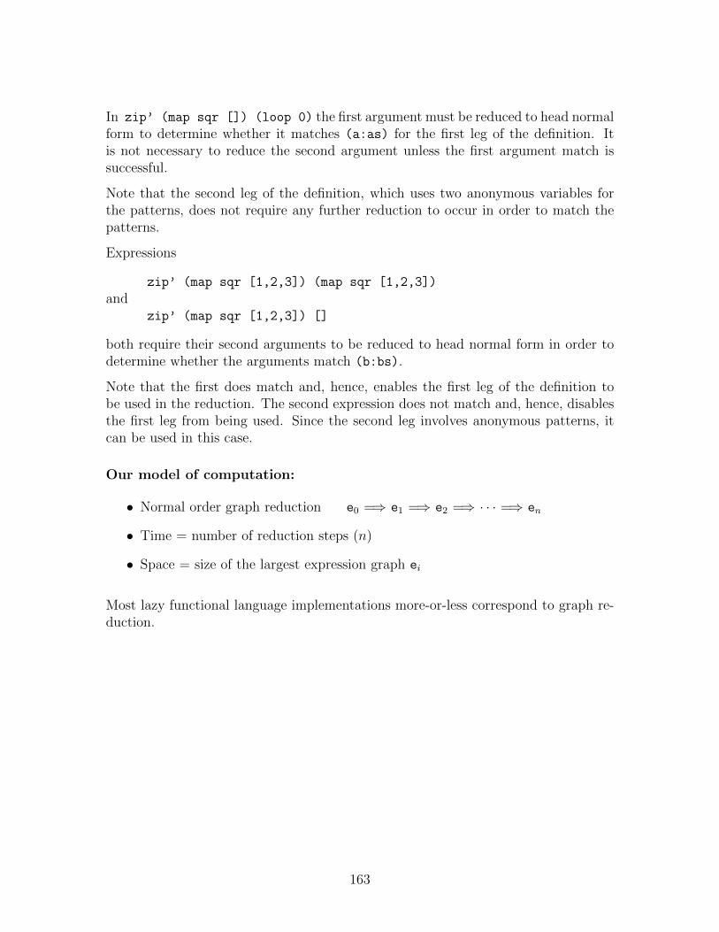
In zip’ (map sqr []) (loop 0) the first argument must be reduced to head normalform to determine whether it matches (a:as) for the first leg of the definition. Itis not necessary to reduce the second argument unless the first argument match issuccessful.

Note that the second leg of the definition, which uses two anonymous variables forthe patterns, does not require any further reduction to occur in order to match thepatterns.

Expressions

zip’ (map sqr [1,2,3]) (map sqr [1,2,3])

andzip’ (map sqr [1,2,3]) []

both require their second arguments to be reduced to head normal form in order todetermine whether the arguments match (b:bs).

Note that the first does match and, hence, enables the first leg of the definition tobe used in the reduction. The second expression does not match and, hence, disablesthe first leg from being used. Since the second leg involves anonymous patterns, itcan be used in this case.

Our model of computation:

• Normal order graph reduction e0 =⇒ e1 =⇒ e2 =⇒ · · · =⇒ en

• Time = number of reduction steps (n)

• Space = size of the largest expression graph ei

Most lazy functional language implementations more-or-less correspond to graph re-duction.

163

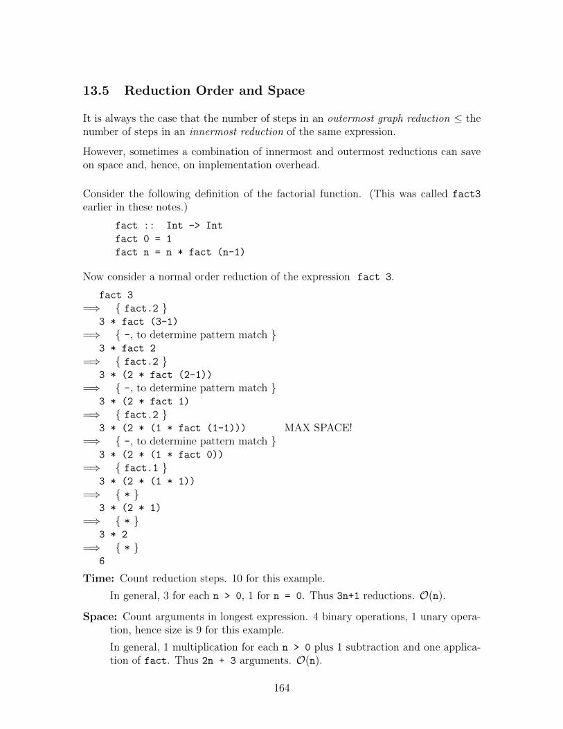
13.5 Reduction Order and Space

It is always the case that the number of steps in an outermost graph reduction ≤ thenumber of steps in an innermost reduction of the same expression.

However, sometimes a combination of innermost and outermost reductions can saveon space and, hence, on implementation overhead.

Consider the following definition of the factorial function. (This was called fact3

earlier in these notes.)

fact :: Int -> Int

fact 0 = 1

fact n = n * fact (n-1)

Now consider a normal order reduction of the expression fact 3.

fact 3

=⇒ { fact.2 }3 * fact (3-1)

=⇒ { -, to determine pattern match }3 * fact 2

=⇒ { fact.2 }3 * (2 * fact (2-1))

=⇒ { -, to determine pattern match }3 * (2 * fact 1)

=⇒ { fact.2 }3 * (2 * (1 * fact (1-1))) MAX SPACE!

=⇒ { -, to determine pattern match }3 * (2 * (1 * fact 0))

=⇒ { fact.1 }3 * (2 * (1 * 1))

=⇒ { * }3 * (2 * 1)

=⇒ { * }3 * 2

=⇒ { * }6

Time: Count reduction steps. 10 for this example.

In general, 3 for each n > 0, 1 for n = 0. Thus 3n+1 reductions. O(n).

Space: Count arguments in longest expression. 4 binary operations, 1 unary opera-tion, hence size is 9 for this example.

In general, 1 multiplication for each n > 0 plus 1 subtraction and one applica-tion of fact. Thus 2n + 3 arguments. O(n).

164

Note that function fact is strict in its argument. That is, evaluation of fact alwaysrequires the evaluation of its argument.

Since the value of the argument expression n-1 in the recursive call is eventuallyneeded (by the pattern match), there is no reason to delay evaluation of the expression.That is, the expression could be evaluated eagerly instead of lazily. Thus any workto save this expression for future evaluation would be avoided.

Delaying the computation of an expression incurs overhead in the implementation.The delayed expression and its calling environment (i.e., the values of variables) mustbe packaged so that evaluation can resume correctly when needed. This packaging—called a closure, suspension, or recipe—requires both space and time to be set up.

Furthermore, delayed expressions can aggravate the problem of space leaks .

The implementation of a lazy functional programming language typically allocatesspace for data dynamically from a memory heap. When the heap is exhausted, theimplementation searches through its structures to recover space that is no longer inuse. This process is usually called garbage collection.

However, sometimes it is very difficult for a garbage collector to determine whetheror not a particular data structure is still needed. The garbage collector thus retainssome unneeded data. These are called space leaks.

Aside: Picture bits of memory oozing out of the program, lost to the program forever.Most of these bits collect in the bit bucket under the computer and are automaticallyrecycled when the interpreter restarts. However, in the past a few of these bitsleaked out into the air, gradually polluting the atmosphere of functional programmingresearch centers. Although it has not be scientifically verified, anecdotal evidencesuggests that the bits leaked from functional programs, when exposed to open minds,metamorphose into a powerful intellectual stimulant. Many imperative programmershave observed that programmers who spend a few weeks in the vicinity of functionalprograms seem to develop a permanent distaste for imperative programs and a strangeenhancement of their mental capacities.

Aside continued: As environmental awareness has grown in the functional program-ming community, the implementors of functional languages have begun to developnew leak-avoiding designs for the language processors and garbage collectors. Nowthe amount of space leakage has been reduced considerably. Although it is still aproblem. Of course, in the meantime a large community of programmers have be-come addicted to the intellectual stimulation of functional programming. The numberof addicts in the USA is small, but growing. FP traffickers have found a number ofways to smuggle their illicit materials into the country. Some are brought in via theInternet from clandestine archives in Europe; a number of professors and studentsare believed to be cultivating a domestic supply. Some are smuggled from Europe

165

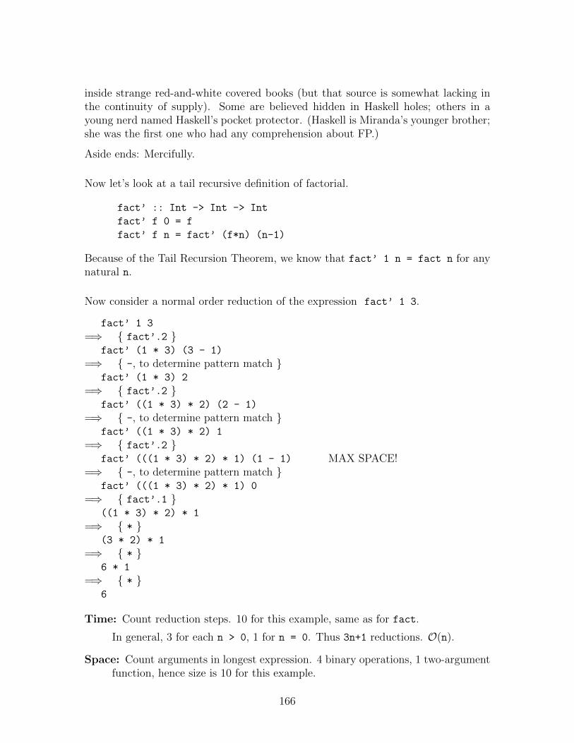
inside strange red-and-white covered books (but that source is somewhat lacking inthe continuity of supply). Some are believed hidden in Haskell holes; others in ayoung nerd named Haskell’s pocket protector. (Haskell is Miranda’s younger brother;she was the first one who had any comprehension about FP.)

Aside ends: Mercifully.

Now let’s look at a tail recursive definition of factorial.

fact’ :: Int -> Int -> Int

fact’ f 0 = f

fact’ f n = fact’ (f*n) (n-1)

Because of the Tail Recursion Theorem, we know that fact’ 1 n = fact n for anynatural n.

Now consider a normal order reduction of the expression fact’ 1 3.

fact’ 1 3

=⇒ { fact’.2 }fact’ (1 * 3) (3 - 1)

=⇒ { -, to determine pattern match }fact’ (1 * 3) 2

=⇒ { fact’.2 }fact’ ((1 * 3) * 2) (2 - 1)

=⇒ { -, to determine pattern match }fact’ ((1 * 3) * 2) 1

=⇒ { fact’.2 }fact’ (((1 * 3) * 2) * 1) (1 - 1) MAX SPACE!

=⇒ { -, to determine pattern match }fact’ (((1 * 3) * 2) * 1) 0

=⇒ { fact’.1 }((1 * 3) * 2) * 1

=⇒ { * }(3 * 2) * 1

=⇒ { * }6 * 1

=⇒ { * }6

Time: Count reduction steps. 10 for this example, same as for fact.

In general, 3 for each n > 0, 1 for n = 0. Thus 3n+1 reductions. O(n).

Space: Count arguments in longest expression. 4 binary operations, 1 two-argumentfunction, hence size is 10 for this example.

166

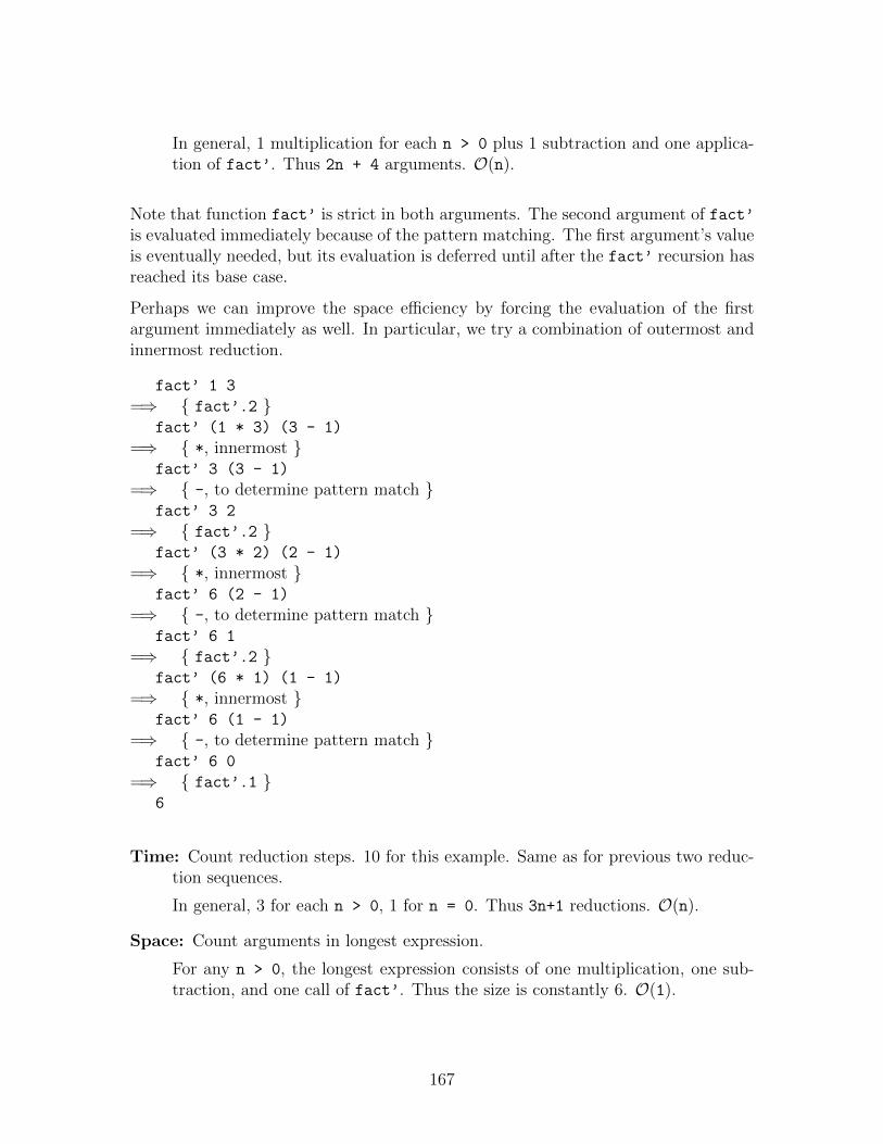
In general, 1 multiplication for each n > 0 plus 1 subtraction and one applica-tion of fact’. Thus 2n + 4 arguments. O(n).

Note that function fact’ is strict in both arguments. The second argument of fact’is evaluated immediately because of the pattern matching. The first argument’s valueis eventually needed, but its evaluation is deferred until after the fact’ recursion hasreached its base case.

Perhaps we can improve the space efficiency by forcing the evaluation of the firstargument immediately as well. In particular, we try a combination of outermost andinnermost reduction.

fact’ 1 3

=⇒ { fact’.2 }fact’ (1 * 3) (3 - 1)

=⇒ { *, innermost }fact’ 3 (3 - 1)

=⇒ { -, to determine pattern match }fact’ 3 2

=⇒ { fact’.2 }fact’ (3 * 2) (2 - 1)

=⇒ { *, innermost }fact’ 6 (2 - 1)

=⇒ { -, to determine pattern match }fact’ 6 1

=⇒ { fact’.2 }fact’ (6 * 1) (1 - 1)

=⇒ { *, innermost }fact’ 6 (1 - 1)

=⇒ { -, to determine pattern match }fact’ 6 0

=⇒ { fact’.1 }6

Time: Count reduction steps. 10 for this example. Same as for previous two reduc-tion sequences.

In general, 3 for each n > 0, 1 for n = 0. Thus 3n+1 reductions. O(n).

Space: Count arguments in longest expression.

For any n > 0, the longest expression consists of one multiplication, one sub-traction, and one call of fact’. Thus the size is constantly 6. O(1).

167

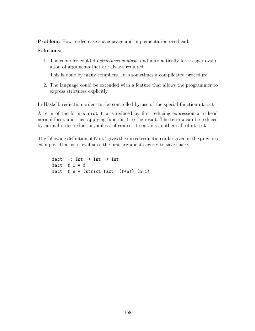
Problem: How to decrease space usage and implementation overhead.

Solutions:

1. The compiler could do strictness analysis and automatically force eager evalu-ation of arguments that are always required.

This is done by many compilers. It is sometimes a complicated procedure.

2. The language could be extended with a feature that allows the programmer toexpress strictness explicitly.

In Haskell, reduction order can be controlled by use of the special function strict.

A term of the form strict f e is reduced by first reducing expression e to headnormal form, and then applying function f to the result. The term e can be reducedby normal order reduction, unless, of course, it contains another call of strict.

The following definition of fact’ gives the mixed reduction order given in the previousexample. That is, it evaluates the first argument eagerly to save space.

fact’ :: Int -> Int -> Int

fact’ f 0 = f

fact’ f n = (strict fact’ (f*n)) (n-1)

168

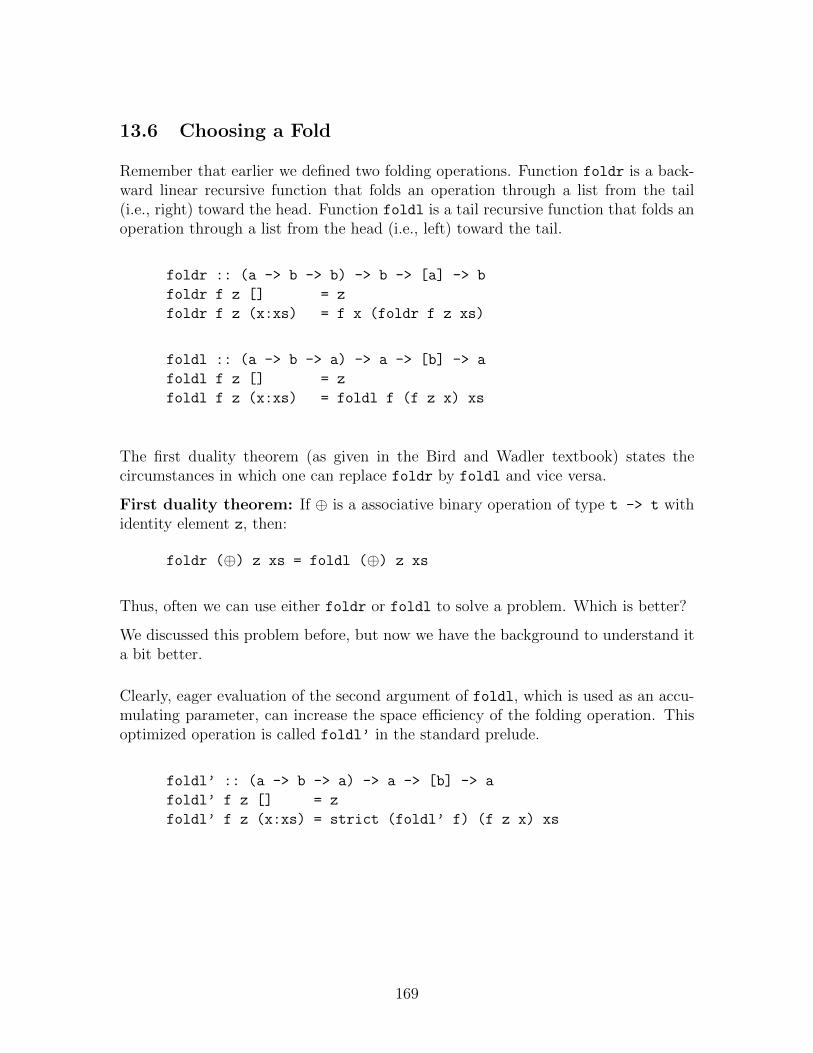
13.6 Choosing a Fold

Remember that earlier we defined two folding operations. Function foldr is a back-ward linear recursive function that folds an operation through a list from the tail(i.e., right) toward the head. Function foldl is a tail recursive function that folds anoperation through a list from the head (i.e., left) toward the tail.

foldr :: (a -> b -> b) -> b -> [a] -> b

foldr f z [] = z

foldr f z (x:xs) = f x (foldr f z xs)

foldl :: (a -> b -> a) -> a -> [b] -> a

foldl f z [] = z

foldl f z (x:xs) = foldl f (f z x) xs

The first duality theorem (as given in the Bird and Wadler textbook) states thecircumstances in which one can replace foldr by foldl and vice versa.

First duality theorem: If ⊕ is a associative binary operation of type t -> t withidentity element z, then:

foldr (⊕) z xs = foldl (⊕) z xs

Thus, often we can use either foldr or foldl to solve a problem. Which is better?

We discussed this problem before, but now we have the background to understand ita bit better.

Clearly, eager evaluation of the second argument of foldl, which is used as an accu-mulating parameter, can increase the space efficiency of the folding operation. Thisoptimized operation is called foldl’ in the standard prelude.

foldl’ :: (a -> b -> a) -> a -> [b] -> a

foldl’ f z [] = z

foldl’ f z (x:xs) = strict (foldl’ f) (f z x) xs

169

Suppose that op is strict in both arguments and can be computed in O(1) time andO(1) space. (For example, + and * have these characteristics.) If n = length xs,then both foldr op i xs and foldl op i xs can be computed in O(n) time andO(n) space.

However, foldl’ op i xs requires O(n) time and O(1) space. The reasoning forthis is similar to that given for fact’.

Thus, in general, foldl’ is the better choice for this case.

Alternatively, suppose that op is nonstrict in either argument . Then foldr is usuallymore efficient than foldl.

As an example, consider operation || (i.e., logical-or). The || operator is strict in thefirst argument, but not in the second. That is, True || x = True without having toevaluate x.

Let xs = [x1, x2, x3, · · ·, xn] such that

(∃ i : 1 ≤ i ≤ n :: xi = True ∧ (∀ j : 1 ≤ j < i :: xj = False))

Suppose xi is the minimum i satisfying the above existential.

foldr (||) False xs

=⇒ { many steps }x1 || (x2 || ( · · · || (xi || ( · · · || (xn || False) · · · )

Because of the nonstrict definition of ||, the above can stop after the xi term isprocessed. None of the list to the right of xi needs to be evaluated.

However, a version which uses foldl must process the entire list.

foldl (||) False xs

=⇒ { many steps }( · · · ( False || x1) || x2) || · · ·) || xi) || · · ·) || xn

In this example, foldr is clearly more efficient than foldl.

170

14 DIVIDE AND CONQUER ALGORITHMS

Reference: This section is based on section 6.4 of the Bird and Wadler textbook [2]and section 4.2 of Kelly’s book Functional Programming for Loosely-coupled Multi-processors [19].

14.1 Overview

General strategy:

1. Decompose problem P into subproblems, each like P but with a smaller inputargument.

2. Solve each subproblem, either directly or by recursively applying the strategy.

3. Assemble the solution to P by combining the solutions to its subproblems.

Advantages:

• Can lead to efficient solutions.

• Allows use of a “horizontal” parallelism. Similar problems can be solved simul-taneously.

Section 6.4 of the Bird and Wadler textbook discusses several important divide andconquer algorithms: mergesort, quicksort, multiplication, and binary search. In thesealgorithms the divide and conquer technique leads to more efficient algorithms.

For example, a simple sequential search is O(n) (where n denotes the length of theinput). Application of the divide and conquer strategy leads to the binary searchwhich is a more efficient O(log2 n) search.

171

As a general pattern of computation, the divide and conquer strategy can be statedwith the following higher order function.

divideAndConquer :: (a -> Bool) -- trivial

-> (a -> b) -- simplySolve

-> (a -> [a]) -- decompose

-> (a -> [b] -> b) -- combineSolutions

-> a -- problem

-> b

divideAndConquer trivial simplySolve decompose

combineSolutions problem

= solve problem

where solve p | trivial p = simplySolve p

| otherwise = combineSolutions p

(map solve (decompose p))

If the problem is trivially simple (i.e., trivial p), then it is solved directly usingsimplySolve.

If the problem is not trivially simple, then it is decomposed into a list of subproblemsusing decompose and each subproblem is solved separately using map solve. The listof solutions to the subproblems are then assembled into a solution for the problemusing combineSolutions. (Sometimes combineSolutions may require the originalproblem description in order to put the solutions back together properly. Hence theparameter p.)

Note that the solution of each subproblem is completely independent from the solutionof all the others. If all the subproblem solutions are needed by combineSolutions,then the language implementation could potentially solve the subproblems simulta-neously. The implementation could take advantage of the availability of multipleprocessors and actually evaluate the expressions in parallel. This is “horizontal”parallelism as described above.

Note: If combineSolutions does not require all the subproblem solutions, thenthe subproblems cannot be safely solved in parallel. If they were, the result ofcombineSolutions might be nondeterministic, that is, the result could be depen-dent upon the relative order in which the subproblem results are completed.

172

14.2 Divide and Conquer Fibonacci

Now let’s use the function divideAndConquer to define a few functions.

First, let’s define a Fibonacci function. (This is adapted from the function definedon pages 77-8 of Kelly [19]. This function is inefficient. It is given here to illustratethe technique.)

fib :: Int -> Int

fib n = divideAndConquer trivial simplySolve decompose

combineSolutions problem

where trivial 0 = True

trivial 1 = True

trivial (m+2) = False

simplySolve 0 = 0

simplySolve 1 = 1

decompose m = [m-1,m-2]

combineSolutions [x,y] = x + y

14.3 Divide and Conquer Folding

Next, let’s consider a folding function (similar to foldr and foldl) that uses thefunction divideAndConquer. (This is adapted from the function defined on pages79-80 of Kelly [19].)

fold :: (a -> a -> a) -> a -> [a] -> a

fold op i = divideAndConquer trivial simplySolve decompose

combineSolutions

where trivial xs = length xs <= 1

simplySolve [] = i

simplySolve [x] = x

decompose xs = [take m xs, drop m xs]

where m = length xs / 2

combineSolutions [x,y] = op x y

This function divides the input list into two almost equal parts, folds each part sepa-rately, and then applies the operation to the two partial results to get the combinedresult.

173

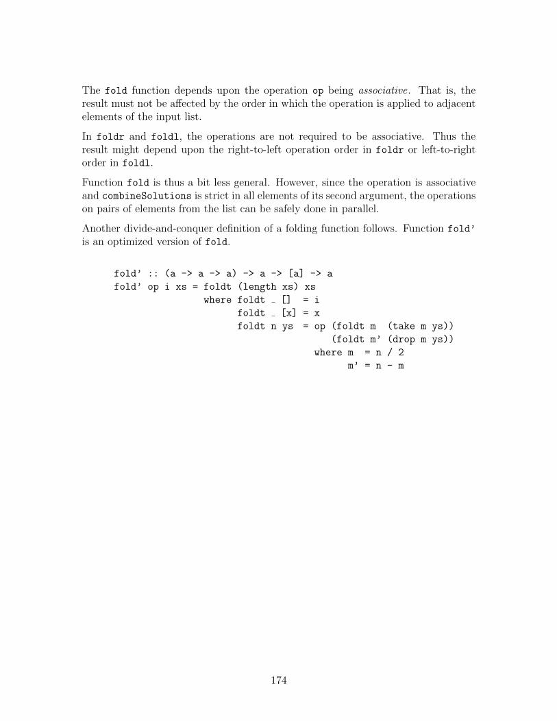
The fold function depends upon the operation op being associative. That is, theresult must not be affected by the order in which the operation is applied to adjacentelements of the input list.

In foldr and foldl, the operations are not required to be associative. Thus theresult might depend upon the right-to-left operation order in foldr or left-to-rightorder in foldl.

Function fold is thus a bit less general. However, since the operation is associativeand combineSolutions is strict in all elements of its second argument, the operationson pairs of elements from the list can be safely done in parallel.

Another divide-and-conquer definition of a folding function follows. Function fold’

is an optimized version of fold.

fold’ :: (a -> a -> a) -> a -> [a] -> a

fold’ op i xs = foldt (length xs) xs

where foldt [] = i

foldt [x] = x

foldt n ys = op (foldt m (take m ys))

(foldt m’ (drop m ys))

where m = n / 2

m’ = n - m

174

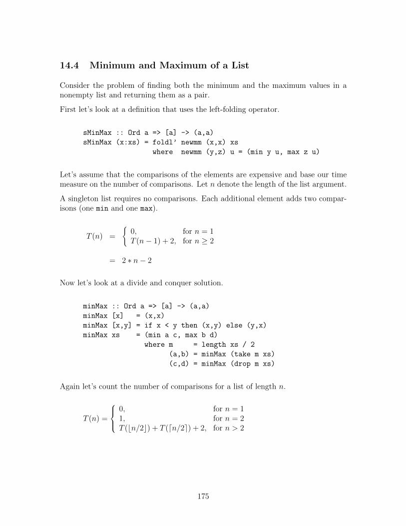
14.4 Minimum and Maximum of a List

Consider the problem of finding both the minimum and the maximum values in anonempty list and returning them as a pair.

First let’s look at a definition that uses the left-folding operator.

sMinMax :: Ord a => [a] -> (a,a)

sMinMax (x:xs) = foldl’ newmm (x,x) xs

where newmm (y,z) u = (min y u, max z u)

Let’s assume that the comparisons of the elements are expensive and base our timemeasure on the number of comparisons. Let n denote the length of the list argument.

A singleton list requires no comparisons. Each additional element adds two compar-isons (one min and one max).

T (n) =

{0, for n = 1T (n− 1) + 2, for n ≥ 2

= 2 ∗ n− 2

Now let’s look at a divide and conquer solution.

minMax :: Ord a => [a] -> (a,a)

minMax [x] = (x,x)

minMax [x,y] = if x < y then (x,y) else (y,x)

minMax xs = (min a c, max b d)

where m = length xs / 2

(a,b) = minMax (take m xs)

(c,d) = minMax (drop m xs)

Again let’s count the number of comparisons for a list of length n.

T (n) =

0, for n = 11, for n = 2T (bn/2c) + T (dn/2e) + 2, for n > 2

175

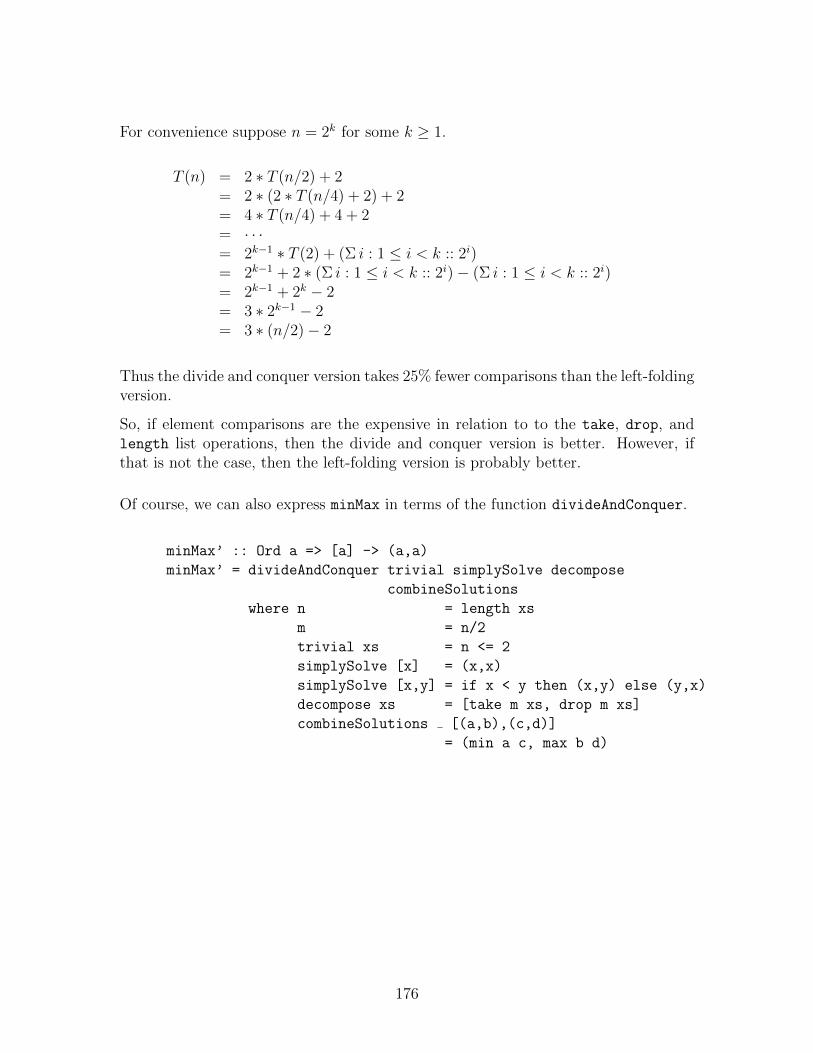
For convenience suppose n = 2k for some k ≥ 1.

T (n) = 2 ∗ T (n/2) + 2= 2 ∗ (2 ∗ T (n/4) + 2) + 2= 4 ∗ T (n/4) + 4 + 2= · · ·= 2k−1 ∗ T (2) + (Σ i : 1 ≤ i < k :: 2i)= 2k−1 + 2 ∗ (Σ i : 1 ≤ i < k :: 2i)− (Σ i : 1 ≤ i < k :: 2i)= 2k−1 + 2k − 2= 3 ∗ 2k−1 − 2= 3 ∗ (n/2)− 2

Thus the divide and conquer version takes 25% fewer comparisons than the left-foldingversion.

So, if element comparisons are the expensive in relation to to the take, drop, andlength list operations, then the divide and conquer version is better. However, ifthat is not the case, then the left-folding version is probably better.

Of course, we can also express minMax in terms of the function divideAndConquer.

minMax’ :: Ord a => [a] -> (a,a)

minMax’ = divideAndConquer trivial simplySolve decompose

combineSolutions

where n = length xs

m = n/2

trivial xs = n <= 2

simplySolve [x] = (x,x)

simplySolve [x,y] = if x < y then (x,y) else (y,x)

decompose xs = [take m xs, drop m xs]

combineSolutions [(a,b),(c,d)]

= (min a c, max b d)

176

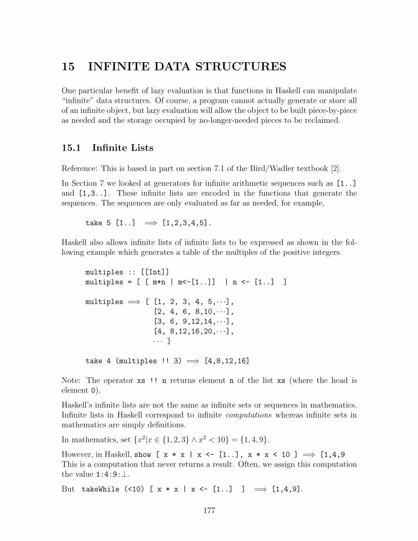
15 INFINITE DATA STRUCTURES

One particular benefit of lazy evaluation is that functions in Haskell can manipulate“infinite” data structures. Of course, a program cannot actually generate or store allof an infinite object, but lazy evaluation will allow the object to be built piece-by-pieceas needed and the storage occupied by no-longer-needed pieces to be reclaimed.

15.1 Infinite Lists

Reference: This is based in part on section 7.1 of the Bird/Wadler textbook [2].

In Section 7 we looked at generators for infinite arithmetic sequences such as [1..]

and [1,3..]. These infinite lists are encoded in the functions that generate thesequences. The sequences are only evaluated as far as needed, for example,

take 5 [1..] =⇒ [1,2,3,4,5].

Haskell also allows infinite lists of infinite lists to be expressed as shown in the fol-lowing example which generates a table of the multiples of the positive integers.

multiples :: [[Int]]

multiples = [ [ m*n | m<-[1..]] | n <- [1..] ]

multiples =⇒ [ [1, 2, 3, 4, 5,· · ·],[2, 4, 6, 8,10,· · ·],[3, 6, 9,12,14,· · ·],[4, 8,12,16,20,· · ·],· · · ]

take 4 (multiples !! 3) =⇒ [4,8,12,16]

Note: The operator xs !! n returns element n of the list xs (where the head iselement 0).

Haskell’s infinite lists are not the same as infinite sets or sequences in mathematics.Infinite lists in Haskell correspond to infinite computations whereas infinite sets inmathematics are simply definitions.

In mathematics, set {x2|x ∈ {1, 2, 3} ∧ x2 < 10} = {1, 4, 9}.

However, in Haskell, show [ x * x | x <- [1..], x * x < 10 ] =⇒ [1,4,9

This is a computation that never returns a result. Often, we assign this computationthe value 1:4:9:⊥.

But takeWhile (<10) [ x * x | x <- [1..] ] =⇒ [1,4,9].

177

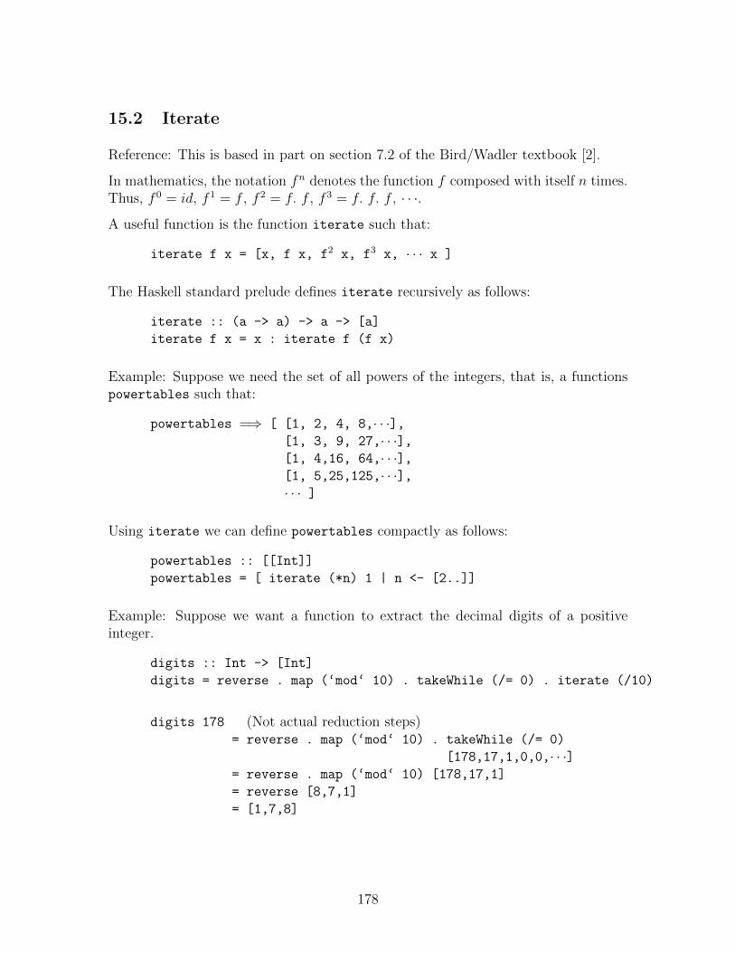
15.2 Iterate

Reference: This is based in part on section 7.2 of the Bird/Wadler textbook [2].

In mathematics, the notation fn denotes the function f composed with itself n times.Thus, f 0 = id, f 1 = f , f 2 = f. f , f 3 = f. f. f , · · ·.

A useful function is the function iterate such that:

iterate f x = [x, f x, f2 x, f3 x, · · · x ]

The Haskell standard prelude defines iterate recursively as follows:

iterate :: (a -> a) -> a -> [a]

iterate f x = x : iterate f (f x)

Example: Suppose we need the set of all powers of the integers, that is, a functionspowertables such that:

powertables =⇒ [ [1, 2, 4, 8,· · ·],[1, 3, 9, 27,· · ·],[1, 4,16, 64,· · ·],[1, 5,25,125,· · ·],· · · ]

Using iterate we can define powertables compactly as follows:

powertables :: [[Int]]

powertables = [ iterate (*n) 1 | n <- [2..]]

Example: Suppose we want a function to extract the decimal digits of a positiveinteger.

digits :: Int -> [Int]

digits = reverse . map (‘mod‘ 10) . takeWhile (/= 0) . iterate (/10)

digits 178 (Not actual reduction steps)= reverse . map (‘mod‘ 10) . takeWhile (/= 0)

[178,17,1,0,0,· · ·]= reverse . map (‘mod‘ 10) [178,17,1]

= reverse [8,7,1]

= [1,7,8]

178

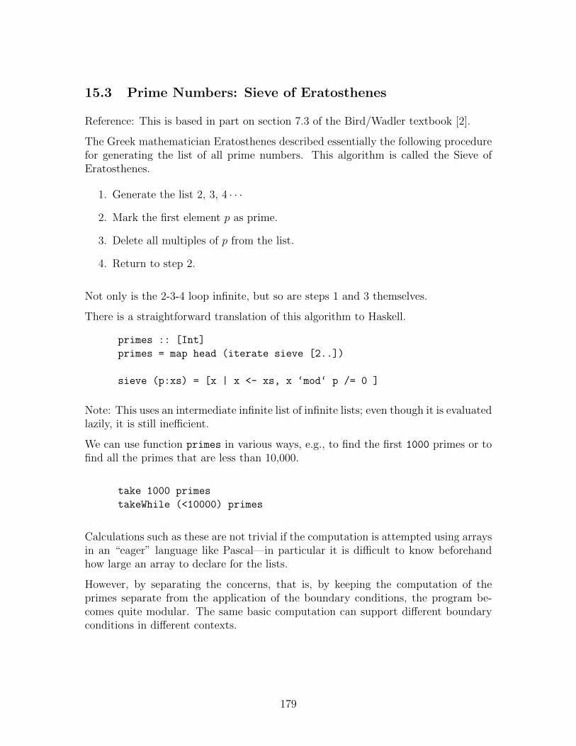
15.3 Prime Numbers: Sieve of Eratosthenes

Reference: This is based in part on section 7.3 of the Bird/Wadler textbook [2].

The Greek mathematician Eratosthenes described essentially the following procedurefor generating the list of all prime numbers. This algorithm is called the Sieve ofEratosthenes.

1. Generate the list 2, 3, 4 · · ·

2. Mark the first element p as prime.

3. Delete all multiples of p from the list.

4. Return to step 2.

Not only is the 2-3-4 loop infinite, but so are steps 1 and 3 themselves.

There is a straightforward translation of this algorithm to Haskell.

primes :: [Int]

primes = map head (iterate sieve [2..])

sieve (p:xs) = [x | x <- xs, x ‘mod‘ p /= 0 ]

Note: This uses an intermediate infinite list of infinite lists; even though it is evaluatedlazily, it is still inefficient.

We can use function primes in various ways, e.g., to find the first 1000 primes or tofind all the primes that are less than 10,000.

take 1000 primes

takeWhile (<10000) primes

Calculations such as these are not trivial if the computation is attempted using arraysin an “eager” language like Pascal—in particular it is difficult to know beforehandhow large an array to declare for the lists.

However, by separating the concerns, that is, by keeping the computation of theprimes separate from the application of the boundary conditions, the program be-comes quite modular. The same basic computation can support different boundaryconditions in different contexts.

179

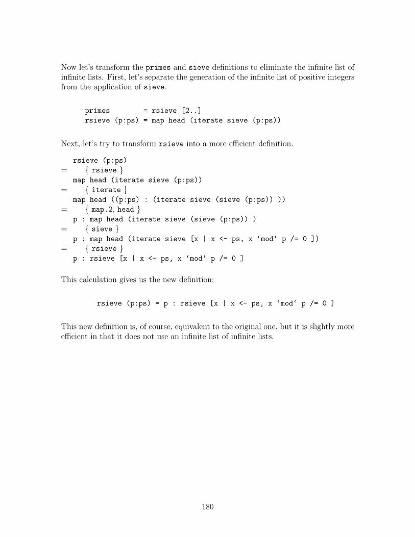
Now let’s transform the primes and sieve definitions to eliminate the infinite list ofinfinite lists. First, let’s separate the generation of the infinite list of positive integersfrom the application of sieve.

primes = rsieve [2..]

rsieve (p:ps) = map head (iterate sieve (p:ps))

Next, let’s try to transform rsieve into a more efficient definition.

rsieve (p:ps)

= { rsieve }map head (iterate sieve (p:ps))

= { iterate }map head ((p:ps) : (iterate sieve (sieve (p:ps)) ))

= { map.2, head }p : map head (iterate sieve (sieve (p:ps)) )

= { sieve }p : map head (iterate sieve [x | x <- ps, x ‘mod‘ p /= 0 ])

= { rsieve }p : rsieve [x | x <- ps, x ‘mod‘ p /= 0 ]

This calculation gives us the new definition:

rsieve (p:ps) = p : rsieve [x | x <- ps, x ‘mod‘ p /= 0 ]

This new definition is, of course, equivalent to the original one, but it is slightly moreefficient in that it does not use an infinite list of infinite lists.

180

.

References

[1] J. Backus. Can programming languages be liberated from the von Neumannstyle? A functional style and its algebra of programs. Communications of theACM, 21(8):613–641, August 1978.

[2] R. Bird and P. Wadler. Introduction to Functional Programming. Prentice HallInternational, New York, 1988.

[3] R. S. Bird. Algebraic identities for program calculation. The Computer Journal,32(2):122–126, 1989.

[4] E. Cohen. Programming in the 1990’s: An Introduction to the Calculation ofPrograms. Springer-Verlag, New York, 1990.

[5] H. C. Cunningham. Notes on functional programming with Gofer. TechnicalReport UMCIS-1995-01, University of Mississippi, Department of Computer andInformation Science, June 1995.

[6] A. Cuoco. Investigations in Algebra. MIT Press, 1990.

[7] A. J. T. Davie. An Introduction to Functional Programming Systems UsingHaskell. Cambridge University Press, 1992.

[8] A. J. Field and P. G. Harrison. Functional Programming. Addison Wesley,Reading, Massachusetts, 1988.

[9] B. Hayes. On the ups and downs of hailstone numbers. Scientific American,250(1):10–16, January 1984.

[10] R. Hoogerwoord. The Design of Functional Programs: A Calculational Approach.PhD thesis, Eindhoven Technical University, Eindhoven, The Netherlands, 1989.

[11] P. Hudak. Conception, evolution, and application of functional programminglanguages. ACM Computing Surveys, 21(3):359–411, September 1989.

[12] P. Hudak and J. H. Fasel. A gentle introduction to Haskell. ACM SIGPLANNOTICES, 27(5), May 1992.

[13] P. Hudak, S. Peyton Jones, and P. Wadler. Report on the programming languageHaskell: A non-strict, purely functional language. ACM SIGPLAN NOTICES,27(5), May 1992.

[14] J. Hughes. Why functional programming matters. The Computer Journal,32(2):98–107, 1989.

181

[15] M. P. Jones. An Introduction to Gofer, 1991. Tutorial manual distributed as apart of the Gofer system beginning with Version 2.20.

[16] S. L. Peyton Jones. The Implementation of Functional Programming Languages.Prentice Hall International, New York, 1987.

[17] S. L. Peyton Jones and D. Lester. Implementing Functional Languages. PrenticeHall International, New York, 1992.

[18] A. Kaldewaij. Programming: The Derivation of Algorithms. Prentice Hall Inter-national, New York, 1990.

[19] P. Kelly. Functional Programming for Loosely-coupled Multiprocessors. MITPress, Cambridge, Massachusetts, 1989.

[20] G. Polya. How to Solve It: A New Aspect of Mathematical Method. PrincetonUnversity Press, second edition, 1957.

[21] G. Polya. Mathematical Discovery: On Understanding, Learning, and TeachingProblem Solving. Wiley, combined edition, 1981.

[22] E. P. Wentworth. Introduction to functional programming using RUFL. Tech-nical Report PPG 89/6, Rhodes University, Department of Computer Science,Grahamstown, South Africa, Revised August 1990.

182

Index

Tf , 149β-reduction, 150⊥ , 61, 150, 154δ-reduction, 150→ , 152∗→ , 152O() , 37, 123, 149product, 60sum, 60++ , 36-> , 17, 26. , 69:: , 17: , 27<- , 80BinTree, 87Bool, 25Char, 25Doc, 77Double, 25False, 25Float, 25Gtree, 91Integer, 25Int, 17, 25Line, 77Matrix, 86Nat, 91Page, 77Point, 86Seq, 92, 93Set, 86String, 27True, 25Word, 77[], 27[m,m’..] , 79[m,m’..n] , 79[m..] , 79[m..n] , 79

&& , 25, 32

car, 27case, 87divide, 86enumFromThenTo, 79enumFromThen, 79enumFromTo, 79enumFrom, 79even, 57flatten, 88foldl’, 61fringe, 89gmerge, 73hailstone, 48if-then-else, 18infixl, 35infixr, 35infix, 35len, 28makeSet, 86merge, 74not, 25nub, 86position, 83sort, 90treeFold, 88rem, 46

** , 136

++ , 109, 111, 113, 147

EDITLINE, see environment variable

EDITOR, see environment variable

Enum, see class

Eq, see class

FailCont, see continuation

Line, 139

Nat, 121

Num, see class

Ord, see class

Para, 144

183

StrCont, see continuation

SuccCont, see continuation

Text, 139

Word, 143

[], 110

abort, see continuation

all, 120

allfacts, 147

allfibs, 126, 127, 129

answer, 153

breakOn, 143

concat, 120

const, see combinator

countLines, 145

countParas, 146

countWords, 146

digits, 178

divideAndConquer, 173

drop, 115, 119, 130, 131

dropWhile, 120

exit, see continuation

exp, 136--138

fact, 164

fastfib, 125

fib, 119, 123, 173

fibs, 126--129

filter, 120

flip, see combinator

fold, 173, 174

foldl, 121, 169

foldl’, 169

foldl1, 140

foldr, 120, 121, 169

foldr1, 140

fst, see combinator

id, see combinator

insert’, 140

iterate, 178

length, 114, 119

let, see local definition

lg, 147

lines, 143

lines’, 139, 140, 143

loop, 153

map, 120

minMax, 175, 176

mul, 147

multiples, 177

normalize, 146

paras’, 145

parse, 146

powertables, 178

primes, 179

rev, 116, 119, 128, 132, 134, 149

reverse, 116, 119, 132, 149

roots, 157

sMinMax, 175

sieve, 179

snd, see combinator

sqr, 151, 155

sqrt, 157

strict, 168

take, 115, 130

takeWhile, 120

twofib, 124, 125

unlines, 143

unlines’, 139, 140

unparas’, 145

unparse, 146

unwords’, 144

where, see local definition

words’, 144

zip, 162

C combinator, see combinator

I combinator, see combinator

K combinator, see combinator

fact

using strict, 168

lines’

specification, 140

Abelian group, 14

absolute value, 45

abstraction, 7, 29, 55, 57, 59

accumulating parameter, 39, 123, 134,

135

accumulator, see accumulating parameter

184

anonymous function, see function

AOR, see applicative order reduction

application, see function

applicative language, see language

applicative order reduction, see reduction

argument, see function

arithmetic sequence, 79

arity, 85

ascending, 73

association order, 35

associative, 14, 30, 111, 174

auxiliary function, 132

AVL, 90

backquote, 41

backslash, 25, 69

Backus, 2

backward recursion, see recursion

bag, 50

Big-O, 37, 123, 149

bijective, 13

binary operation, 14, 35, 59

binary tree, see tree

binding order, 35

Boolean, 25

bottom, 61

call-by-name, 154

call-by-need, 154, 155

call-by-value, 154

canonical form, 44

character, 25

literal, 25

newline, 25, 139

special, 25

Church-Rosser Theorem, 152

class, 33

Enum, 79

Eq, 33

Num, 45, 79

Ord, 33, 79

closure, 165

codomain, 13

combinator, 65

. , 66

C, 65

I, 65

K, 65

flip, 65

fst, 65

id, 66

snd, 65

fst, 151

id, 119

thd3, 127

command, 5

comment, 31

commutative, 14

complexity ordering, 109

composition, see operator

comprehension, see list

computational model, 163

cons, 27, see list

constant function, 65

construct, 5

constructor, see list, see operator

context predicate, 33, see class

Control-D, see character

Control-Z, see character

cosequential processing, 73--75

Curry, 26, 63

currying, 26, 62

data constant, 85

data constructor, see operator

declarative, 5

decreasing, 73

decreasing space, 168

derivation, see program synthesis

descending, 73

Diamond Property, 152

divide and conquer, 108, 171--176

as higher-order function, 172

strategy, 108, 171

divide-by-zero error, 86

domain, 13

duality theorem, 60, 169

185

eager evaluation, see evaluation

efficiency, 149

end-of-file, see character

enumerated type, see type

equational reasoning, 16, 111

equivalence, 116, 131

equivalence of definitions, 16

Eratosthenes, 179

error termination, 45

evaluation, 150

eager, iv, 8, 154, 168

lazy, iii, 8, 154, 177

exponentiation, see operator

expression, 5

expression evaluator, 54

expression recognizer, 53

extensionality, 63

factorial, 17--21, 52, 147, 164, 166

failure continuation, see continuation

Fibonacci sequence, 41, 52, 119, 123--129,

173

filter, 57

finite list, 109

first duality theorem, 60, 169

first-class function, see function

first-order function, see function

floating point, 25

fold, 58, 59, 173

choosing left or right, 61, 169

divide-and-conquer, 174

left, 60, 140

optimized left, 169

right, 59, 140

tree, 88

forward recursion, see recursion

free binding, 35

FreeBSD, iii

function, 5, 13, 26

anonymous, 69

application, 13, 18, 19

argument, 18, 159

call, see application

composition, 13, 66, 119, 120

declaration, 18

definition, 15, 17, 31, 40, 69

equivalence, 116--118

first-class, 7, 26

first-order, 55

higher-order, 7, 55, 63

local definition, see local definition

name, 18, 26

paraneter, 18

result, 13, 18

well-defined, 17

functional programming, 1

functional language, see language

garbage collection, 165

geometric sequence, 79

GHC, 1

Gofer interpreter, iii

acquiring, iii

library, see prelude

graph reduction, 1, see reduction

greatest common divisor, 45

group, 14

guard, 19, 33

Haskell, iii, 1, see language

Haskell interpreter

library, 27

prelude

standard, 27

reduction, 155

Haskell Platform, 1

head, 27

head normal form, 160

heap, 165

heuristic, 106, 117

higher-order function, see function

I/O, see input/output

identity, 14, 17, 30, 59, 113

left, 14, 60

right, 14, 59

identity function, 65

imperative, 5

186

increasing, 49, 73

indentation, 18

induction, 15--16, 109--110, 124

base case, 15, 110, 124

hypothesis, 15, 110, 124

inductive case, 15, 110, 124

list, 110

mathematical, 15

natural number, 15

proof strategy, 110

structural, 109

well-founded, 132, 133

infinite data structure, 8, 177

infinite set, 177

infix, 14, 18, 27, 35, 41

injective, 13

innermost reduction, see reduction

insert, 59

integer, 25

integer division, 138

interpreter, 23

inverse, 13, 14

left, 14

right, 14

invertible, 13

iteration, 16

Jones, Mark, iii

juxtaposition, 19, 63

lambda expression, 69

language

applicative, 5, see functional

declarative, 5

FP, 4, 5

functional, 5

Gofer, iii

Haskell, iii, 1, 5

Hope, iv, 5

imperative, 5

Lisp, 5

logic, 6

Miranda, 5

non-von Neumann, 4

Orwell, 5

paradigm, 5

Prolog, 6

relational, 6

RUFL, iii

Scheme, 5

SML, 5

von Neumann, 3, 5

law, 6, 109, 119

singleton, 118, 119

lazy evaluation, see evaluation

leftmost reduction, see reduction

leg, 31

lenient, see strictness

library, see Hugs interpreter

line, 139

processing, 139--143

separator, 139

terminator, 143

linear recursion, see recursion

list, 27, 92, 93

append, 36, 109, 111--113

breaking operator, 43, 69

combining operator, 44, 70

comprehension, 80

expression, 80

filter, 80

generator, 80

local definition, 80

qualifier, 80

cons, see constructor

constructor, 27, 110

element selection operator, 43

head, 27

infinite, 8, 79, 177

maximum, 175

merge, 73

minimum, 175

nil, 27, 110

reverse, 37--40, 116--118, 132

tail, 27

literate script, see Hugs interpreter

local definition, 39

187

local definition, 40

let, 40

where, 39, 41

let, 156

where, 156

bottom-up, 40

effect on efficiency, 156

top-down, 41

logarithm, 147

logarithmic algorithm, 137

map, 55

mathematical induction, see induction

modularity, 8

monoid, 14, 37, 60, 109, 121

MS-DOS, iii

multiset, 50

multiway tree, see tree

natural number, 15, 17, 91

unbounded precision, 51

nondeterministic, 172

nonstrict, see strictness

NOR, see normal order reduction

normal form, 44, 150, 153

normal order reduction, see reduction

nullary, 85

number base conversion, 49

one-to-one, 13

one-to-one correspondence, 13

onto, 13

operator

and, 25

binary, see binary operation

data constructor, 85

data constructor, 89

exclusive-or, 48

exponentiation, 35, 136

list, see list

not, 25

or, 25

precedence, 35

section, 64

outermost reduction, see reduction

paragraph, 144

processing, 144--145

parallelism, 9, 174

horizontal, 171, 172

parameter, see function

partial function, 13

partial application, 26, 62

pattern matching, 70

(n+k) pattern, 20

pattern matching, 19

effect on reduction, 162

integer, 19

list, 30, 32, 34

order of testing, 19, 31, 74

reduction rule, 162

wildcard, 32

pattern of computation, 55

Polya, 105

polymorphic type, see type

predicate, 6

prefix, 18, 76

prelude, see Gofer interpreter

prime number, 81, 179

problem solving, 105--108

program derivation, see program synthesis

program synthesis, 123

strategy, 125

programming, 1, 105

project file, see Gofer interpreter

Prolog, see language

proof, 109, 123

quadratic formula, 157

range, 13

rational number arithmetic, 44--119

real number, 25

recipe, 165

record, 29

recurrence relation, 15, 17

recursion, 5, 16

backward, 38, 132, 135

188

forward, 38

linear, 38, 132, 135

tail, 38, 132, 135, see Tail Recursion

Theorem

recursive definition, 15, 17

redex, 150

reduce, 59

reduction, 150--168

AOR, see applicative order

applicative order, 151, 154, 155

graph, 155, 163, 164

innermost, 150, 164

leftmost, 150, 155

NOR, see normal order

normal order, 151, 153--155, 162,

163

outermost, 150, 155, 164

rightmost, 150

string, 155

termination of, 162

reduction relation, 152

referential transparency, 6, 9, 109,

154

reflexive transitive closure, 152

relation, 6

relatively prime, 45

remainder, 46

replace constant by variable, 117

replace equals by equals, 109

reuse standard solutions, 107

rewriting, 150

rightmost reduction, see reduction

script, see Gofer interpreter

seed, 59, 60, 140

segment, 76

semigroup, 14

separate concerns, 108, 179

sequencing, 5

set, 49

side effect, 5, 154

Sieve of Eratosthenes, 179

sign, 45

simplification, 110, 111, 150

size of expression, 159, 163

solve a harder problem, 83, 106, 117,

125

solve a related problem, 107

solve a simpler problem, 107

space complexity, 135, 149, 159, 163

space leaks, 165

specification, 123

standard prelude, see Gofer interpreter

state, 5

implicit, 5

no implicit, 5

strict, see strictness

strictness, 61, 135, 137

strict, 168

analysis, 168

exploiting, 167--169

lenient, 61, 154

nonstrict, 61, 154

strict, 61, 154

string, 27

literal, 28

string reduction, see reduction

structural induction, see induction

structure, 29

success continuation, see continuation

suffix, 76

surjective, 13

suspension, 165

symmetric, 14

synonym, see type

synthesis, see program synthesis

tail, 27

tail recursion, see recursion

Tail Recursion Theorem, 132--136

generalization, 147

text, 139

justification, 52

processing, 139--146

time complexity, 135, 149, 163

total function, 13

transitive closure, 152

traversal, 88, 90

189

tree, 87

binary, 87, 89

binary search, 90

general, 91

height, 90

multiway, 91

perfectly balanced, 90

truncation, 138

tuple type, see type

tupling, 123, 126, 128

type, 25, 85

(t1,t2,· · ·,tn), 29

Bool, 25

Char, 25

Double, 25

Float, 25

Integer, 25

Int, 25

String, 27

built-in, 25

enumerated, 79, 85

function, 26

list, 27

polymorphic, 29

recursive, 87

signature, 17

synonym, 27, 86

tree, 87

tuple, 29, 86

union, 86

user-defined, 25, 85

type variable, 29

unbounded precision arithmetic, 51

Unicode, 25

union type, see type

unit, 14

UNIX, iii

variable

name, 26

von Neumann, 2

bottleneck, 2

computer, 2

language, 3, 5

non-von Neumann language, 4

wildcard, see pattern matching

word, 143

processing, 143--144

word equivalent, 77

world of expressions, 4

world of statements, 4

zero, 14

left, 14

right, 14

190