Getting Started in R~Stata Notes on Exploring Data

(v. 1.0)

Oscar Torres-Reyna otorres@princeton.edu

http://dss.princeton.edu/training/ Fall 2010

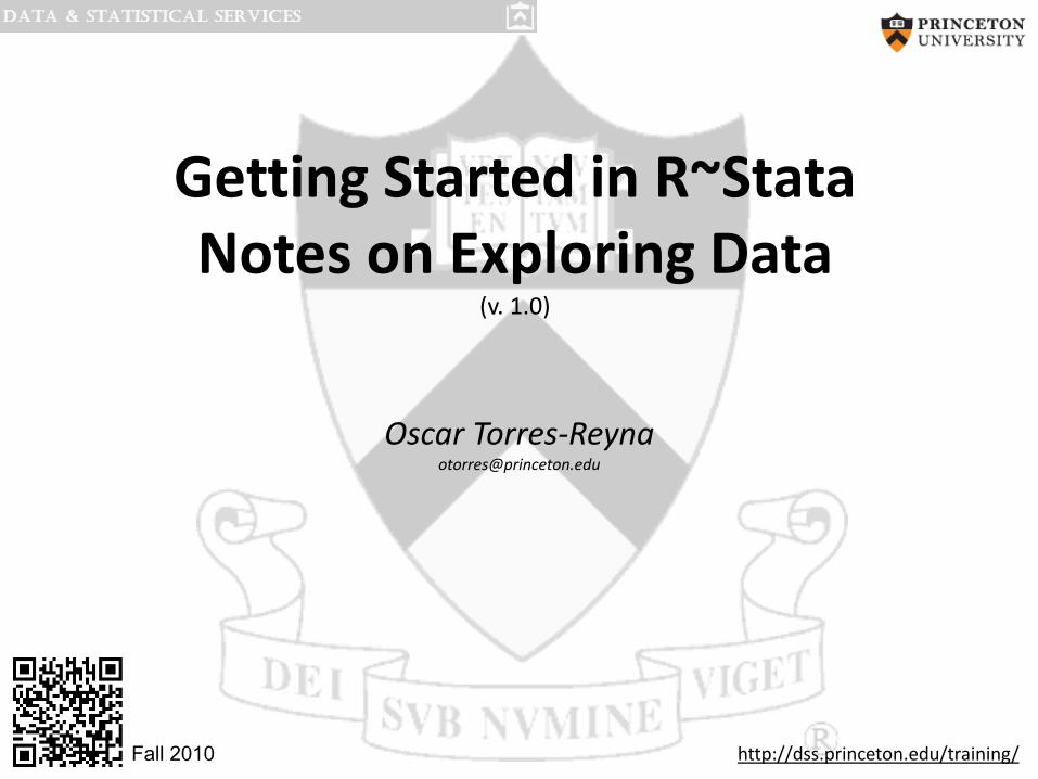
What is R/Stata?What is R?• “R is a language and environment for statistical computing and graphics”*• R is offered as open source (i.e. free)What is Stata?• It is a multi-purpose statistical package to help you explore, summarize and analyze datasets. • A dataset is a collection of several pieces of information called variables (usually arranged by

columns). A variable can have one or several values (information for one or several cases).• Other statistical packages are SPSS and SAS.

Features Stata SPSS SAS R

Learning curve Steep/gradual Gradual/flat Pretty steep Pretty steep

User interface Programming/point-and-click Mostly point-and-click Programming Programming

Data manipulation Very strong Moderate Very strong Very strong

Data analysis Powerful Powerful Powerful/versatile Powerful/versatile

Graphics Very good Very good Good Excellent

CostAffordable (perpetual

licenses, renew only when upgrade)

Expensive (but not need to renew until upgrade, long

term licenses)

Expensive (yearly renewal) Open source

* http://www.r-project.org/index.html

NOTE: The R content presented in this document is mostly based on an early version of Fox, J. and Weisberg, S. (2011) An R Companion to Applied Regression, Second Edition, Sage; and from class notes from the ICPSR’s workshop Introduction to the R Statistical Computing Environment taught by John Fox during the summer of 2010.

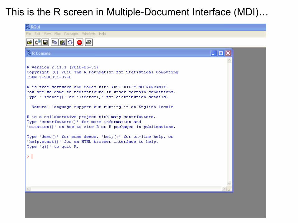
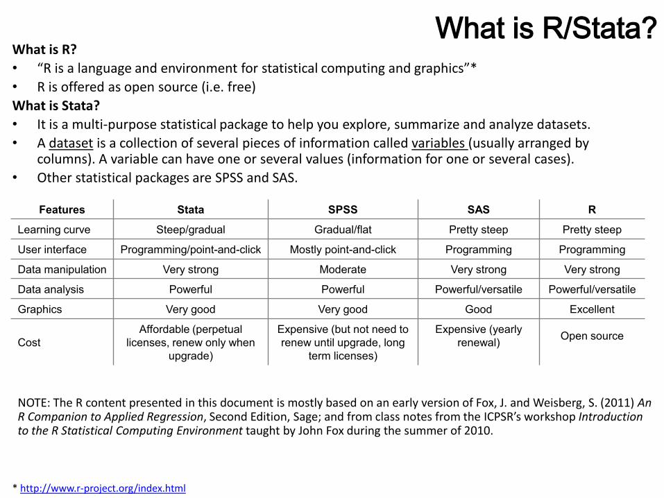
This is the R screen in Multiple-Document Interface (MDI)…

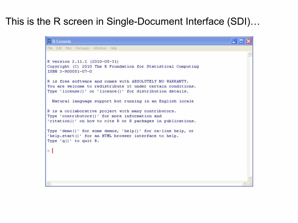
This is the R screen in Single-Document Interface (SDI)…

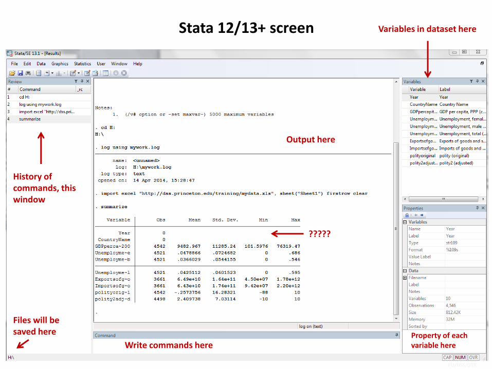
Stata 12/13+ screen

Write commands here

Files will be saved here

History of commands, this window

Output here

Variables in dataset here

Property of each variable here

?????

PU/DSS/OTR

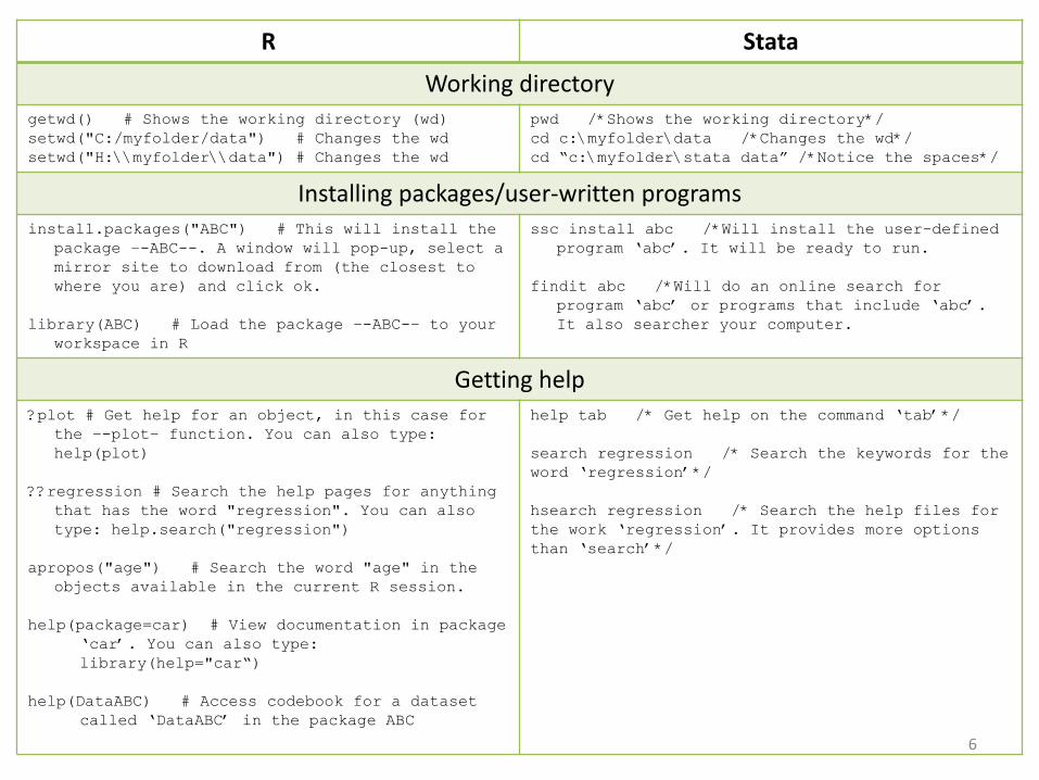
R Stata

Working directorygetwd() # Shows the working directory (wd)setwd("C:/myfolder/data") # Changes the wdsetwd("H:\\myfolder\\data") # Changes the wd

pwd /*Shows the working directory*/cd c:\myfolder\data /*Changes the wd*/cd “c:\myfolder\stata data” /*Notice the spaces*/

Installing packages/user-written programsinstall.packages("ABC") # This will install the

package –-ABC--. A window will pop-up, select a mirror site to download from (the closest to where you are) and click ok.

library(ABC) # Load the package –-ABC-– to your workspace in R

ssc install abc /*Will install the user-defined program ‘abc’. It will be ready to run.

findit abc /*Will do an online search for program ‘abc’ or programs that include ‘abc’. It also searcher your computer.

Getting help?plot # Get help for an object, in this case for

the –-plot– function. You can also type: help(plot)

??regression # Search the help pages for anything that has the word "regression". You can also type: help.search("regression")

apropos("age") # Search the word "age" in the objects available in the current R session.

help(package=car) # View documentation in package ‘car’. You can also type:library(help="car“)

help(DataABC) # Access codebook for a dataset called ‘DataABC’ in the package ABC

help tab /* Get help on the command ‘tab’*/

search regression /* Search the keywords for the word ‘regression’*/

hsearch regression /* Search the help files for the work ‘regression’. It provides more options than ‘search’*/

6

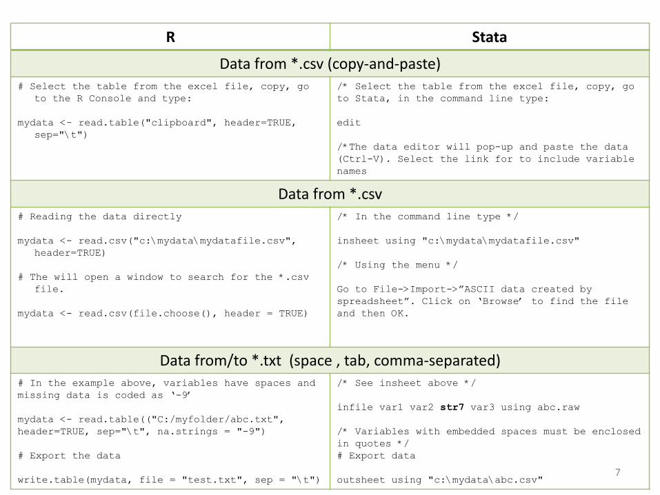
R Stata

Data from *.csv (copy-and-paste)# Select the table from the excel file, copy, go

to the R Console and type:

mydata <- read.table("clipboard", header=TRUE, sep="\t")

/* Select the table from the excel file, copy, go to Stata, in the command line type:

edit

/*The data editor will pop-up and paste the data (Ctrl-V). Select the link for to include variable names

Data from *.csv# Reading the data directly

mydata <- read.csv("c:\mydata\mydatafile.csv", header=TRUE)

# The will open a window to search for the *.csv file.

mydata <- read.csv(file.choose(), header = TRUE)

/* In the command line type */

insheet using "c:\mydata\mydatafile.csv"

/* Using the menu */

Go to File->Import->”ASCII data created by spreadsheet”. Click on ‘Browse’ to find the file and then OK.

Data from/to *.txt (space , tab, comma-separated)# In the example above, variables have spaces and missing data is coded as ‘-9’

mydata <- read.table(("C:/myfolder/abc.txt", header=TRUE, sep="\t", na.strings = "-9")

# Export the data

write.table(mydata, file = "test.txt", sep = "\t")

/* See insheet above */

infile var1 var2 str7 var3 using abc.raw

/* Variables with embedded spaces must be enclosed in quotes */# Export data

outsheet using "c:\mydata\abc.csv"7

R Stata

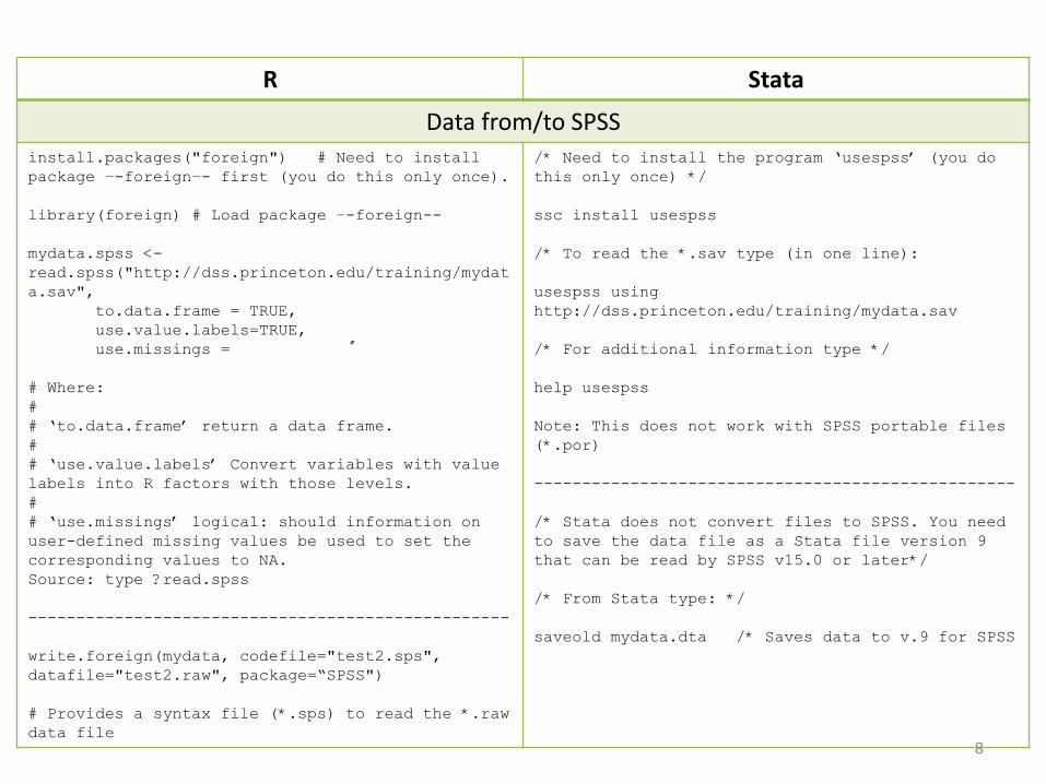
Data from/to SPSSinstall.packages("foreign") # Need to install package –-foreign–- first (you do this only once).

library(foreign) # Load package –-foreign--

mydata.spss <-read.spss("http://dss.princeton.edu/training/mydata.sav",

to.data.frame = TRUE, use.value.labels=TRUE, use.missings = to.data.frame)

# Where:## ‘to.data.frame’ return a data frame.## ‘use.value.labels’ Convert variables with value labels into R factors with those levels.## ‘use.missings’ logical: should information on user-defined missing values be used to set the corresponding values to NA. Source: type ?read.spss

--------------------------------------------------

write.foreign(mydata, codefile="test2.sps", datafile="test2.raw", package=“SPSS")

# Provides a syntax file (*.sps) to read the *.raw data file

/* Need to install the program ‘usespss’ (you do this only once) */

ssc install usespss

/* To read the *.sav type (in one line):

usespss using http://dss.princeton.edu/training/mydata.sav

/* For additional information type */

help usespss

Note: This does not work with SPSS portable files (*.por)

--------------------------------------------------

/* Stata does not convert files to SPSS. You need to save the data file as a Stata file version 9 that can be read by SPSS v15.0 or later*/

/* From Stata type: */

saveold mydata.dta /* Saves data to v.9 for SPSS

8

R Stata

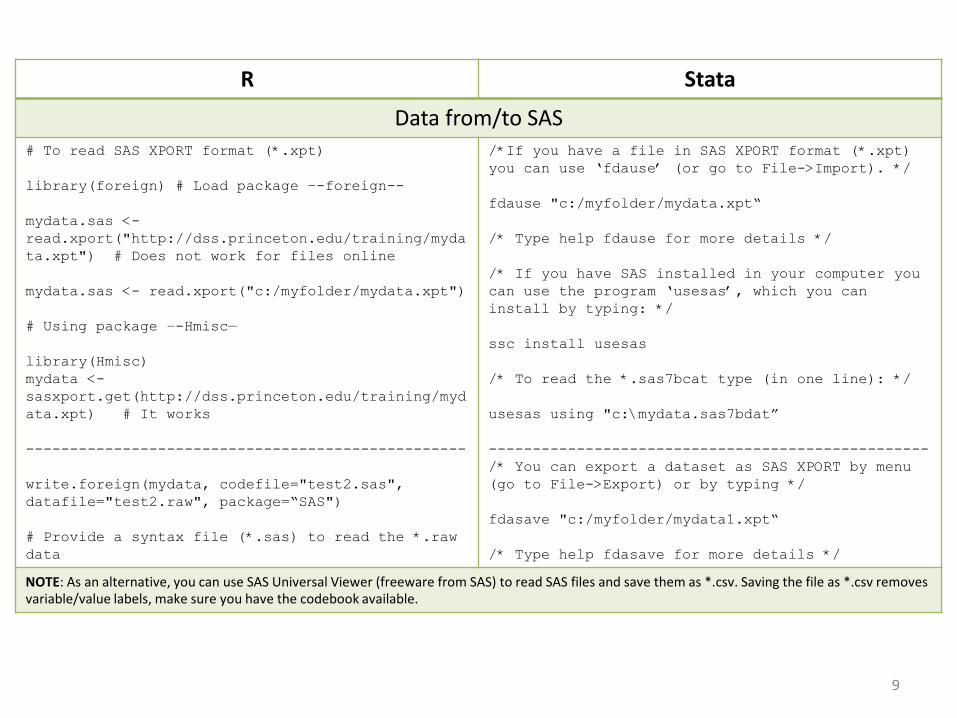
Data from/to SAS# To read SAS XPORT format (*.xpt)

library(foreign) # Load package –-foreign--

mydata.sas <-read.xport("http://dss.princeton.edu/training/mydata.xpt") # Does not work for files online

mydata.sas <- read.xport("c:/myfolder/mydata.xpt")

# Using package –-Hmisc—

library(Hmisc) mydata <-sasxport.get(http://dss.princeton.edu/training/mydata.xpt) # It works

--------------------------------------------------

write.foreign(mydata, codefile="test2.sas", datafile="test2.raw", package=“SAS")

# Provide a syntax file (*.sas) to read the *.raw data

/*If you have a file in SAS XPORT format (*.xpt)you can use ‘fdause’ (or go to File->Import). */

fdause "c:/myfolder/mydata.xpt“

/* Type help fdause for more details */

/* If you have SAS installed in your computer you can use the program ‘usesas’, which you can install by typing: */

ssc install usesas

/* To read the *.sas7bcat type (in one line): */

usesas using "c:\mydata.sas7bdat”

--------------------------------------------------/* You can export a dataset as SAS XPORT by menu (go to File->Export) or by typing */

fdasave "c:/myfolder/mydata1.xpt“

/* Type help fdasave for more details */

NOTE: As an alternative, you can use SAS Universal Viewer (freeware from SAS) to read SAS files and save them as *.csv. Saving the file as *.csv removes variable/value labels, make sure you have the codebook available.

9

R Stata

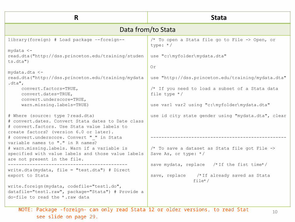
Data from/to Statalibrary(foreign) # Load package –-foreign--

mydata <-read.dta("http://dss.princeton.edu/training/students.dta")

mydata.dta <-read.dta("http://dss.princeton.edu/training/mydata.dta",

convert.factors=TRUE, convert.dates=TRUE, convert.underscore=TRUE, warn.missing.labels=TRUE)

# Where (source: type ?read.dta)# convert.dates. Convert Stata dates to Date class# convert.factors. Use Stata value labels to create factors? (version 6.0 or later).# convert.underscore. Convert "_" in Stata variable names to "." in R names?# warn.missing.labels. Warn if a variable is specified with value labels and those value labels are not present in the file.--------------------------------------------write.dta(mydata, file = "test.dta") # Direct export to Stata

write.foreign(mydata, codefile="test1.do", datafile="test1.raw", package="Stata") # Provide a do-file to read the *.raw data

/* To open a Stata file go to File -> Open, or type: */

use "c:\myfolder\mydata.dta"

Or

use "http://dss.princeton.edu/training/mydata.dta"

/* If you need to load a subset of a Stata data file type */

use var1 var2 using "c:\myfolder\mydata.dta"

use id city state gender using "mydata.dta", clear

--------------------------------------------------

/* To save a dataset as Stata file got File -> Save As, or type: */

save mydata, replace /*If the fist time*/

save, replace /*If already saved as Stata file*/

10

R Stata

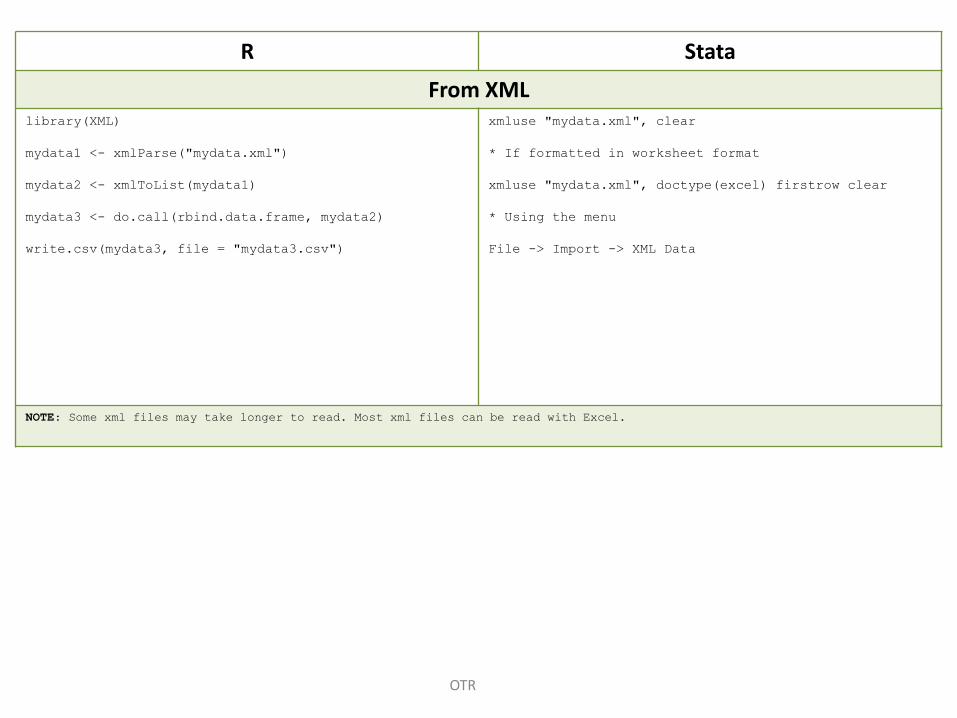
From XML library(XML)

mydata1 <- xmlParse("mydata.xml")

mydata2 <- xmlToList(mydata1)

mydata3 <- do.call(rbind.data.frame, mydata2)

write.csv(mydata3, file = "mydata3.csv")

xmluse "mydata.xml", clear

* If formatted in worksheet format

xmluse "mydata.xml", doctype(excel) firstrow clear

* Using the menu

File -> Import -> XML Data

NOTE: Some xml files may take longer to read. Most xml files can be read with Excel.

OTR

R Stata

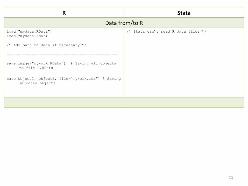
Data from/to Rload("mydata.RData")load("mydata.rda")

/* Add path to data if necessary */

-------------------------------------------------

save.image("mywork.RData") # Saving all objects to file *.RData

save(object1, object2, file=“mywork.rda") # Saving selected objects

/* Stata can’t read R data files */

11

R Stata

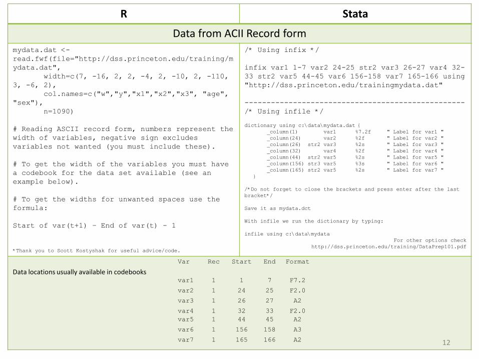
Data from ACII Record formmydata.dat <-read.fwf(file="http://dss.princeton.edu/training/mydata.dat",

width=c(7, -16, 2, 2, -4, 2, -10, 2, -110, 3, -6, 2),

col.names=c("w","y","x1","x2","x3", "age", "sex"),

n=1090)

# Reading ASCII record form, numbers represent the width of variables, negative sign excludes variables not wanted (you must include these).

# To get the width of the variables you must have a codebook for the data set available (see an example below).

# To get the widths for unwanted spaces use the formula:

Start of var(t+1) – End of var(t) - 1

*Thank you to Scott Kostyshak for useful advice/code.

/* Using infix */

infix var1 1-7 var2 24-25 str2 var3 26-27 var4 32-33 str2 var5 44-45 var6 156-158 var7 165-166 using "http://dss.princeton.edu/trainingmydata.dat"

--------------------------------------------------/* Using infile */

dictionary using c:\data\mydata.dat {_column(1) var1 %7.2f " Label for var1 "_column(24) var2 %2f " Label for var2 "_column(26) str2 var3 %2s " Label for var3 "_column(32) var4 %2f " Label for var4 "_column(44) str2 var5 %2s " Label for var5 "_column(156) str3 var5 %3s " Label for var6 "_column(165) str2 var5 %2s " Label for var7 "

}

/*Do not forget to close the brackets and press enter after the last bracket*/

Save it as mydata.dct

With infile we run the dictionary by typing:

infile using c:\data\mydataFor other options check

http://dss.princeton.edu/training/DataPrep101.pdf

Data locations usually available in codebooks

Var Rec Start End Format

var1 1 1 7 F7.2

var2 1 24 25 F2.0

var3 1 26 27 A2

var4 1 32 33 F2.0var5 1 44 45 A2

var6 1 156 158 A3

var7 1 165 166 A2 12

R Stata

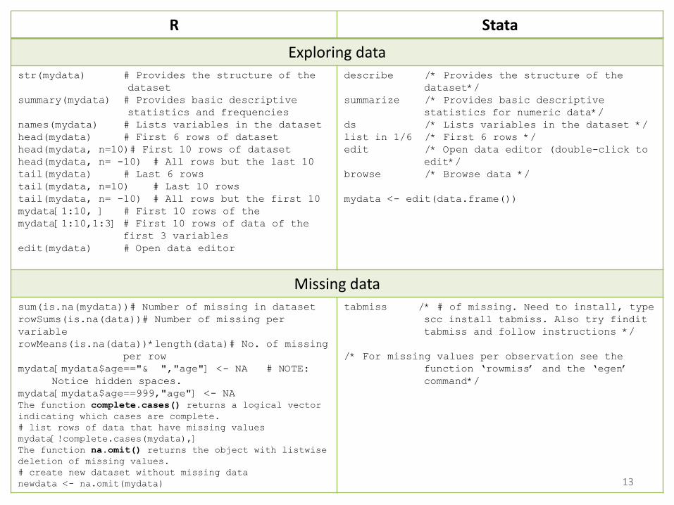
Exploring datastr(mydata) # Provides the structure of the

datasetsummary(mydata) # Provides basic descriptive

statistics and frequenciesnames(mydata) # Lists variables in the datasethead(mydata) # First 6 rows of datasethead(mydata, n=10)# First 10 rows of datasethead(mydata, n= -10) # All rows but the last 10tail(mydata) # Last 6 rowstail(mydata, n=10) # Last 10 rowstail(mydata, n= -10) # All rows but the first 10mydata[1:10, ] # First 10 rows of themydata[1:10,1:3] # First 10 rows of data of the

first 3 variablesedit(mydata) # Open data editor

describe /* Provides the structure of the dataset*/

summarize /* Provides basic descriptive statistics for numeric data*/

ds /* Lists variables in the dataset */list in 1/6 /* First 6 rows */edit /* Open data editor (double-click to

edit*/browse /* Browse data */

mydata <- edit(data.frame())

Missing datasum(is.na(mydata))# Number of missing in datasetrowSums(is.na(data))# Number of missing per variablerowMeans(is.na(data))*length(data)# No. of missing

per rowmydata[mydata$age=="& ","age"] <- NA # NOTE:

Notice hidden spaces.mydata[mydata$age==999,"age"] <- NAThe function complete.cases() returns a logical vector indicating which cases are complete. # list rows of data that have missing values mydata[!complete.cases(mydata),]The function na.omit() returns the object with listwisedeletion of missing values. # create new dataset without missing data newdata <- na.omit(mydata)

tabmiss /* # of missing. Need to install, type scc install tabmiss. Also try findittabmiss and follow instructions */

/* For missing values per observation see the function ‘rowmiss’ and the ‘egen’ command*/

13

R Stata

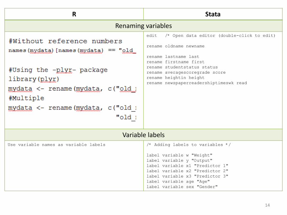
Renaming variables#Using base commands

fix(mydata) # Rename interactively.names(mydata)[3] <- "First"

# Using library –-reshape--

library(reshape)

mydata <- rename(mydata, c(Last.Name="Last"))mydata <- rename(mydata, c(First.Name="First"))mydata <- rename(mydata,

c(Student.Status="Status"))mydata <- rename(mydata,

c(Average.score..grade.="Score"))mydata <- rename(mydata, c(Height..in.="Height"))mydata <- rename(mydata,

c(Newspaper.readership..times.wk.="Read"))

edit /* Open data editor (double-click to edit)

rename oldname newname

rename lastname lastrename firstname firstrename studentstatus statusrename averagescoregrade scorerename heightin heightrename newspaperreadershiptimeswk read

Variable labelsUse variable names as variable labels /* Adding labels to variables */

label variable w "Weight"label variable y "Output"label variable x1 "Predictor 1"label variable x2 "Predictor 2"label variable x3 "Predictor 3"label variable age "Age"label variable sex "Gender"

14

R Stata

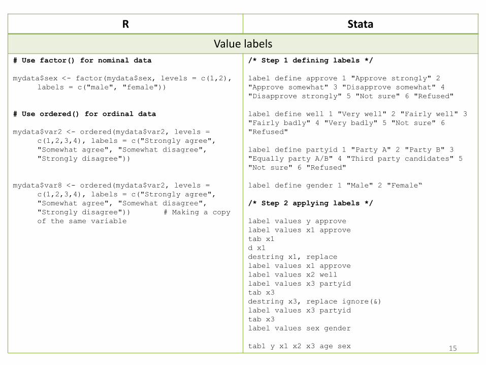
Value labels# Use factor() for nominal data

mydata$sex <- factor(mydata$sex, levels = c(1,2), labels = c("male", "female"))

# Use ordered() for ordinal data

mydata$var2 <- ordered(mydata$var2, levels = c(1,2,3,4), labels = c("Strongly agree", "Somewhat agree", "Somewhat disagree", "Strongly disagree"))

mydata$var8 <- ordered(mydata$var2, levels = c(1,2,3,4), labels = c("Strongly agree", "Somewhat agree", "Somewhat disagree", "Strongly disagree")) # Making a copyof the same variable

/* Step 1 defining labels */

label define approve 1 "Approve strongly" 2 "Approve somewhat" 3 "Disapprove somewhat" 4 "Disapprove strongly" 5 "Not sure" 6 "Refused"

label define well 1 "Very well" 2 "Fairly well" 3 "Fairly badly" 4 "Very badly" 5 "Not sure" 6 "Refused"

label define partyid 1 "Party A" 2 "Party B" 3 "Equally party A/B" 4 "Third party candidates" 5 "Not sure" 6 "Refused"

label define gender 1 "Male" 2 "Female“

/* Step 2 applying labels */

label values y approvelabel values x1 approvetab x1d x1destring x1, replacelabel values x1 approvelabel values x2 welllabel values x3 partyidtab x3destring x3, replace ignore(&)label values x3 partyidtab x3label values sex gender

tab1 y x1 x2 x3 age sex 15

R Stata

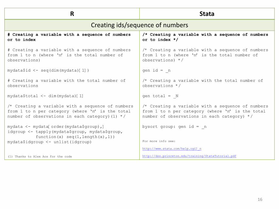
Creating ids/sequence of numbers# Creating a variable with a sequence of numbersor to index

# Creating a variable with a sequence of numbersfrom 1 to n (where ‘n’ is the total number of observations)

mydata$id <- seq(dim(mydata)[1])

# Creating a variable with the total number of observations

mydata$total <- dim(mydata)[1]

/* Creating a variable with a sequence of numbersfrom 1 to n per category (where ‘n’ is the total number of observations in each category)(1) */

mydata <- mydata[order(mydata$group),]idgroup <- tapply(mydata$group, mydata$group,

function(x) seq(1,length(x),1))mydata$idgroup <- unlist(idgroup)

(1) Thanks to Alex Acs for the code

/* Creating a variable with a sequence of numbersor to index */

/* Creating a variable with a sequence of numbersfrom 1 to n (where ‘n’ is the total number of observations) */

gen id = _n

/* Creating a variable with the total number of observations */

gen total = _N

/* Creating a variable with a sequence of numbersfrom 1 to n per category (where ‘n’ is the total number of observations in each category) */

bysort group: gen id = _n

For more info see:

http://www.stata.com/help.cgi?_n

http://dss.princeton.edu/training/StataTutorial.pdf

16

R Stata

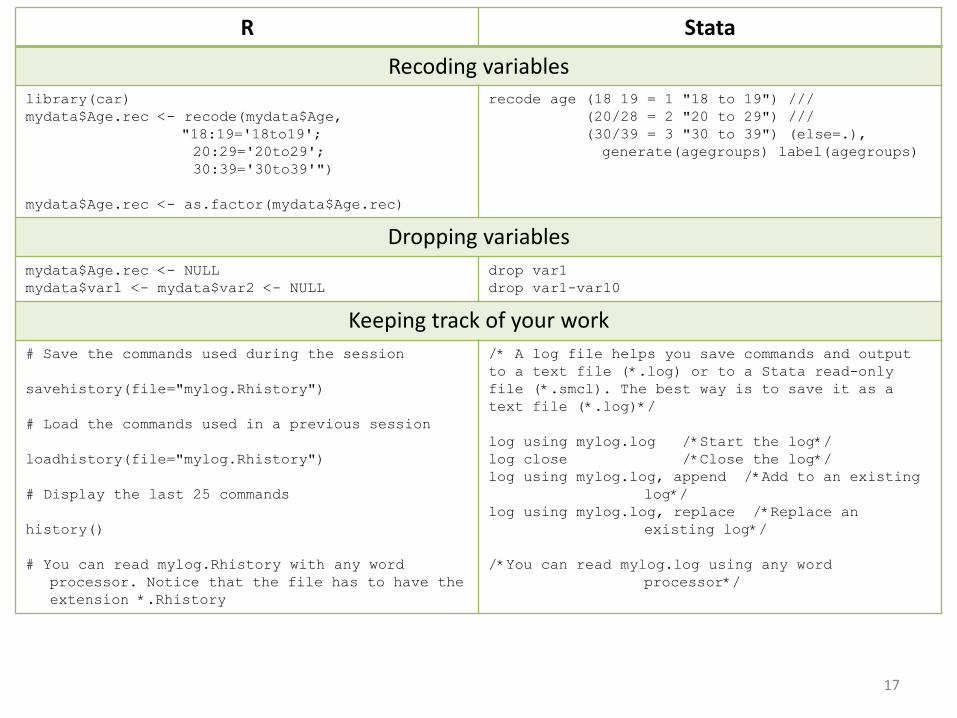
Recoding variableslibrary(car)mydata$Age.rec <- recode(mydata$Age,

"18:19='18to19'; 20:29='20to29';30:39='30to39'")

mydata$Age.rec <- as.factor(mydata$Age.rec)

recode age (18 19 = 1 "18 to 19") ///(20/28 = 2 "20 to 29") ///(30/39 = 3 "30 to 39") (else=.), generate(agegroups) label(agegroups)

Dropping variablesmydata$Age.rec <- NULLmydata$var1 <- mydata$var2 <- NULL

drop var1drop var1-var10

Keeping track of your work# Save the commands used during the session

savehistory(file="mylog.Rhistory")

# Load the commands used in a previous session

loadhistory(file="mylog.Rhistory")

# Display the last 25 commands

history()

# You can read mylog.Rhistory with any word processor. Notice that the file has to have the extension *.Rhistory

/* A log file helps you save commands and output to a text file (*.log) or to a Stata read-only file (*.smcl). The best way is to save it as a text file (*.log)*/

log using mylog.log /*Start the log*/log close /*Close the log*/log using mylog.log, append /*Add to an existing

log*/log using mylog.log, replace /*Replace an

existing log*/

/*You can read mylog.log using any word processor*/

17

R Stata

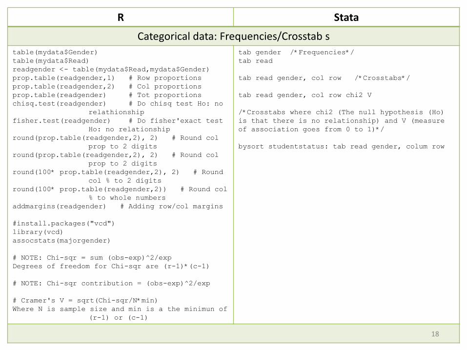
Categorical data: Frequencies/Crosstab stable(mydata$Gender)table(mydata$Read)readgender <- table(mydata$Read,mydata$Gender)prop.table(readgender,1) # Row proportionsprop.table(readgender,2) # Col proportionsprop.table(readgender) # Tot proportionschisq.test(readgender) # Do chisq test Ho: no

relathionshipfisher.test(readgender) # Do fisher'exact test

Ho: no relationshipround(prop.table(readgender,2), 2) # Round col

prop to 2 digitsround(prop.table(readgender,2), 2) # Round col

prop to 2 digitsround(100* prop.table(readgender,2), 2) # Round

col % to 2 digitsround(100* prop.table(readgender,2)) # Round col

% to whole numbersaddmargins(readgender) # Adding row/col margins

#install.packages("vcd")library(vcd)assocstats(majorgender)

# NOTE: Chi-sqr = sum (obs-exp)^2/expDegrees of freedom for Chi-sqr are (r-1)*(c-1)

# NOTE: Chi-sqr contribution = (obs-exp)^2/exp

# Cramer's V = sqrt(Chi-sqr/N*min)Where N is sample size and min is a the minimun of

(r-1) or (c-1)

tab gender /*Frequencies*/tab read

tab read gender, col row /*Crosstabs*/

tab read gender, col row chi2 V

/*Crosstabs where chi2 (The null hypothesis (Ho) is that there is no relationship) and V (measure of association goes from 0 to 1)*/

bysort studentstatus: tab read gender, colum row

18

R Stata

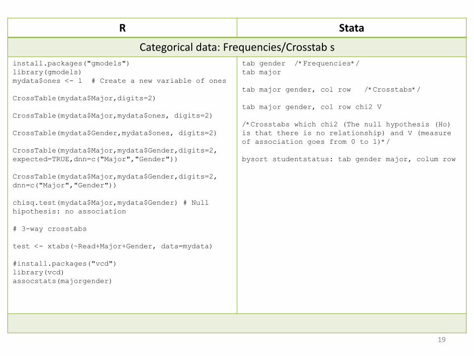
Categorical data: Frequencies/Crosstab sinstall.packages("gmodels")library(gmodels)mydata$ones <- 1 # Create a new variable of ones

CrossTable(mydata$Major,digits=2)

CrossTable(mydata$Major,mydata$ones, digits=2)

CrossTable(mydata$Gender,mydata$ones, digits=2)

CrossTable(mydata$Major,mydata$Gender,digits=2, expected=TRUE,dnn=c("Major","Gender"))

CrossTable(mydata$Major,mydata$Gender,digits=2, dnn=c("Major","Gender"))

chisq.test(mydata$Major,mydata$Gender) # Null hipothesis: no association

# 3-way crosstabs

test <- xtabs(~Read+Major+Gender, data=mydata)

#install.packages("vcd")library(vcd)assocstats(majorgender)

tab gender /*Frequencies*/tab major

tab major gender, col row /*Crosstabs*/

tab major gender, col row chi2 V

/*Crosstabs which chi2 (The null hypothesis (Ho) is that there is no relationship) and V (measure of association goes from 0 to 1)*/

bysort studentstatus: tab gender major, colum row

19

R Stata

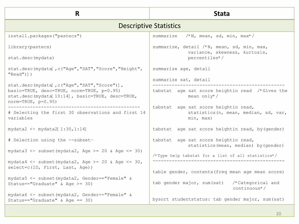
Descriptive Statisticsinstall.packages("pastecs")

library(pastecs)

stat.desc(mydata)

stat.desc(mydata[,c("Age","SAT","Score","Height", "Read")])

stat.desc(mydata[,c("Age","SAT","Score")], basic=TRUE, desc=TRUE, norm=TRUE, p=0.95)stat.desc(mydata[10:14], basic=TRUE, desc=TRUE, norm=TRUE, p=0.95)------------------------------------------------# Selecting the first 30 observations and first 14 variables

mydata2 <- mydata2[1:30,1:14]

# Selection using the --subset—

mydata3 <- subset(mydata2, Age >= 20 & Age <= 30)

mydata4 <- subset(mydata2, Age >= 20 & Age <= 30, select=c(ID, First, Last, Age))

mydata5 <- subset(mydata2, Gender=="Female" & Status=="Graduate" & Age >= 30)

mydata6 <- subset(mydata2, Gender=="Female" & Status=="Graduate" & Age == 30)

summarize /*N, mean, sd, min, max*/

summarize, detail /*N, mean, sd, min, max, variance, skewness, kurtosis, percentiles*/

summarize age, detail

summarize sat, detail------------------------------------------------tabstat age sat score heightin read /*Gives the

mean only*/

tabstat age sat score heightin read, statistics(n, mean, median, sd, var, min, max)

tabstat age sat score heightin read, by(gender)

tabstat age sat score heightin read, statistics(mean, median) by(gender)

/*Type help tabstat for a list of all statistics*/------------------------------------------------

table gender, contents(freq mean age mean score)

tab gender major, sum(sat) /*Categorical and continuous*/

bysort studentstatus: tab gender major, sum(sat)

20

R Stata

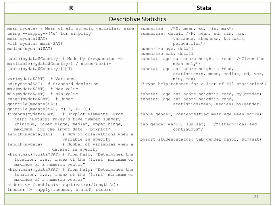
Descriptive Statisticsmean(mydata) # Mean of all numeric variables, same using --sapply--('s' for simplify)mean(mydata$SAT)with(mydata, mean(SAT))median(mydata$SAT)

table(mydata$Country) # Mode by frequencies -> max(table(mydata$Country)) / names(sort(-table(mydata$Country)))[1]

var(mydata$SAT) # Variancesd(mydata$SAT) # Standard deviationmax(mydata$SAT) # Max valuemin(mydata$SAT) # Min valuerange(mydata$SAT) # Rangequantile(mydata$SAT) quantile(mydata$SAT, c(.3,.6,.9))fivenum(mydata$SAT) # Boxplot elements. From

help: "Returns Tukey's five number summary (minimum, lower-hinge, median, upper-hinge, maximum) for the input data ~ boxplot"

length(mydata$SAT) # Num of observations when a variable is specify

length(mydata) # Number of variables when a dataset is specify

which.max(mydata$SAT) # From help: "Determines the location, i.e., index of the (first) minimum or maximum of a numeric vector"

which.min(mydata$SAT) # From help: "Determines the location, i.e., index of the (first) minimum or maximum of a numeric vector”

stderr <- function(x) sqrt(var(x)/length(x)) incster <- tapply(incomes, statef, stderr)

summarize /*N, mean, sd, min, max*/summarize, detail /*N, mean, sd, min, max,

variance, skewness, kurtosis, percentiles*/

summarize age, detailsummarize sat, detailtabstat age sat score heightin read /*Gives the

mean only*/tabstat age sat score heightin read,

statistics(n, mean, median, sd, var, min, max)

/*Type help tabstat for a list of all statistics*/

tabstat age sat score heightin read, by(gender)tabstat age sat score heightin read,

statistics(mean, median) by(gender)

table gender, contents(freq mean age mean score)

tab gender major, sum(sat) /*Categorical and continuous*/

bysort studentstatus: tab gender major, sum(sat)

21

R Stata

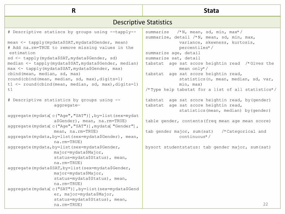
Descriptive Statistics# Descriptive statiscs by groups using --tapply--

mean <- tapply(mydata$SAT,mydata$Gender, mean)# Add na.rm=TRUE to remove missing values in the estimationsd <- tapply(mydata$SAT,mydata$Gender, sd)median <- tapply(mydata$SAT,mydata$Gender, median)max <- tapply(mydata$SAT,mydata$Gender, max)cbind(mean, median, sd, max)round(cbind(mean, median, sd, max),digits=1)t1 <- round(cbind(mean, median, sd, max),digits=1)t1

# Descriptive statistics by groups using --aggregate—

aggregate(mydata[c("Age","SAT")],by=list(sex=mydata$Gender), mean, na.rm=TRUE)

aggregate(mydata[c("Age","SAT")],mydata["Gender"], mean, na.rm=TRUE)

aggregate(mydata,by=list(sex=mydata$Gender), mean, na.rm=TRUE)

aggregate(mydata,by=list(sex=mydata$Gender, major=mydata$Major, status=mydata$Status), mean, na.rm=TRUE)

aggregate(mydata$SAT,by=list(sex=mydata$Gender, major=mydata$Major, status=mydata$Status), mean, na.rm=TRUE)

aggregate(mydata[c("SAT")],by=list(sex=mydata$Gender, major=mydata$Major, status=mydata$Status), mean, na.rm=TRUE)

summarize /*N, mean, sd, min, max*/summarize, detail /*N, mean, sd, min, max,

variance, skewness, kurtosis, percentiles*/

summarize age, detailsummarize sat, detailtabstat age sat score heightin read /*Gives the

mean only*/tabstat age sat score heightin read,

statistics(n, mean, median, sd, var, min, max)

/*Type help tabstat for a list of all statistics*/

tabstat age sat score heightin read, by(gender)tabstat age sat score heightin read,

statistics(mean, median) by(gender)

table gender, contents(freq mean age mean score)

tab gender major, sum(sat) /*Categorical and continuous*/

bysort studentstatus: tab gender major, sum(sat)

22

R Stata

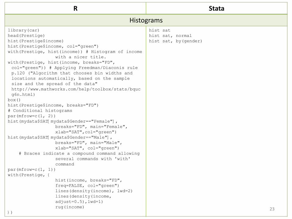
Histogramslibrary(car)head(Prestige)hist(Prestige$income)hist(Prestige$income, col="green")with(Prestige, hist(income)) # Histogram of income

with a nicer title.with(Prestige, hist(income, breaks="FD", col="green")) # Applying Freedman/Diaconis rule p.120 ("Algorithm that chooses bin widths and locations automatically, based on the sample size and the spread of the data" http://www.mathworks.com/help/toolbox/stats/bqucg6n.html)

box()hist(Prestige$income, breaks="FD")# Conditional histograms par(mfrow=c(1, 2))hist(mydata$SAT[mydata$Gender=="Female"],

breaks="FD", main="Female", xlab="SAT",col="green")

hist(mydata$SAT[mydata$Gender=="Male"], breaks="FD", main="Male", xlab="SAT", col="green")

# Braces indicate a compound command allowing several commands with 'with' command

par(mfrow=c(1, 1))with(Prestige, {

hist(income, breaks="FD", freq=FALSE, col="green")lines(density(income), lwd=2)lines(density(income, adjust=0.5),lwd=1)rug(income)

})

hist sathist sat, normalhist sat, by(gender)

23

R Stata

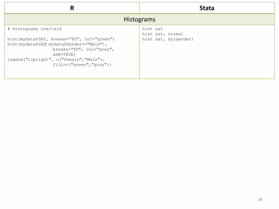
Histograms# Histograms overlaid

hist(mydata$SAT, breaks="FD", col="green")hist(mydata$SAT[mydata$Gender=="Male"],

breaks="FD", col="gray", add=TRUE)

legend("topright", c("Female","Male"), fill=c("green","gray"))

hist sathist sat, normalhist sat, by(gender)

24

R Stata

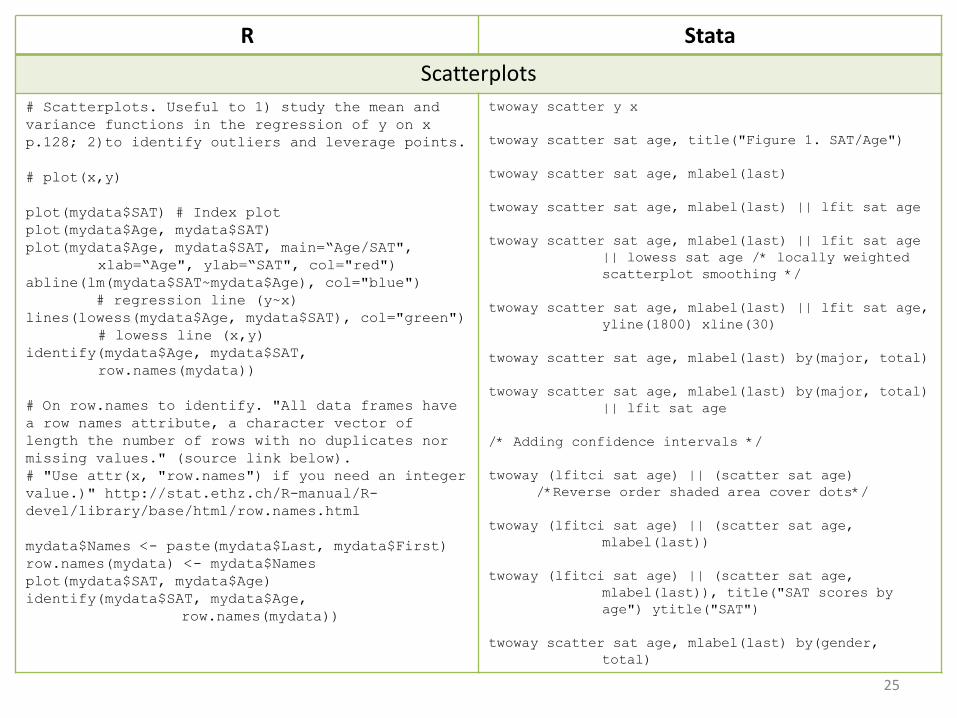
Scatterplots# Scatterplots. Useful to 1) study the mean and variance functions in the regression of y on x p.128; 2)to identify outliers and leverage points.

# plot(x,y)

plot(mydata$SAT) # Index plotplot(mydata$Age, mydata$SAT)plot(mydata$Age, mydata$SAT, main=“Age/SAT",

xlab=“Age", ylab=“SAT", col="red")abline(lm(mydata$SAT~mydata$Age), col="blue")

# regression line (y~x)lines(lowess(mydata$Age, mydata$SAT), col="green")

# lowess line (x,y) identify(mydata$Age, mydata$SAT,

row.names(mydata))

# On row.names to identify. "All data frames have a row names attribute, a character vector of length the number of rows with no duplicates nor missing values." (source link below).# "Use attr(x, "row.names") if you need an integer value.)" http://stat.ethz.ch/R-manual/R-devel/library/base/html/row.names.html

mydata$Names <- paste(mydata$Last, mydata$First)row.names(mydata) <- mydata$Namesplot(mydata$SAT, mydata$Age)identify(mydata$SAT, mydata$Age,

row.names(mydata))

twoway scatter y x

twoway scatter sat age, title("Figure 1. SAT/Age")

twoway scatter sat age, mlabel(last)

twoway scatter sat age, mlabel(last) || lfit sat age

twoway scatter sat age, mlabel(last) || lfit sat age || lowess sat age /* locally weighted scatterplot smoothing */

twoway scatter sat age, mlabel(last) || lfit sat age, yline(1800) xline(30)

twoway scatter sat age, mlabel(last) by(major, total)

twoway scatter sat age, mlabel(last) by(major, total) || lfit sat age

/* Adding confidence intervals */

twoway (lfitci sat age) || (scatter sat age) /*Reverse order shaded area cover dots*/

twoway (lfitci sat age) || (scatter sat age, mlabel(last))

twoway (lfitci sat age) || (scatter sat age, mlabel(last)), title("SAT scores by age") ytitle("SAT")

twoway scatter sat age, mlabel(last) by(gender, total)

25

R Stata

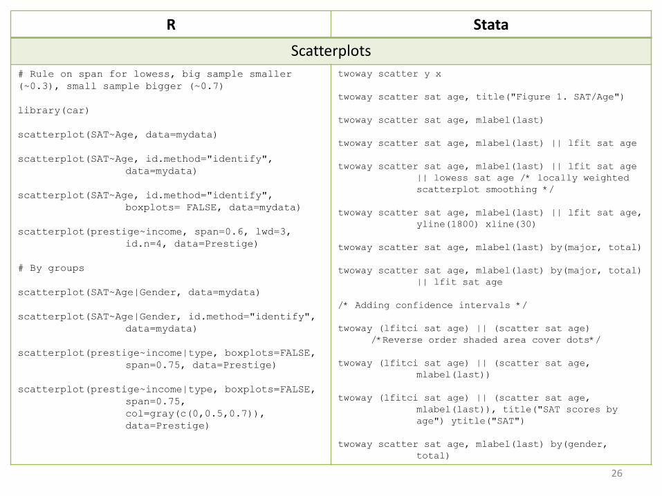
Scatterplots# Rule on span for lowess, big sample smaller (~0.3), small sample bigger (~0.7)

library(car)

scatterplot(SAT~Age, data=mydata)

scatterplot(SAT~Age, id.method="identify", data=mydata)

scatterplot(SAT~Age, id.method="identify", boxplots= FALSE, data=mydata)

scatterplot(prestige~income, span=0.6, lwd=3, id.n=4, data=Prestige)

# By groups

scatterplot(SAT~Age|Gender, data=mydata)

scatterplot(SAT~Age|Gender, id.method="identify", data=mydata)

scatterplot(prestige~income|type, boxplots=FALSE, span=0.75, data=Prestige)

scatterplot(prestige~income|type, boxplots=FALSE, span=0.75, col=gray(c(0,0.5,0.7)), data=Prestige)

twoway scatter y x

twoway scatter sat age, title("Figure 1. SAT/Age")

twoway scatter sat age, mlabel(last)

twoway scatter sat age, mlabel(last) || lfit sat age

twoway scatter sat age, mlabel(last) || lfit sat age || lowess sat age /* locally weighted scatterplot smoothing */

twoway scatter sat age, mlabel(last) || lfit sat age, yline(1800) xline(30)

twoway scatter sat age, mlabel(last) by(major, total)

twoway scatter sat age, mlabel(last) by(major, total) || lfit sat age

/* Adding confidence intervals */

twoway (lfitci sat age) || (scatter sat age) /*Reverse order shaded area cover dots*/

twoway (lfitci sat age) || (scatter sat age, mlabel(last))

twoway (lfitci sat age) || (scatter sat age, mlabel(last)), title("SAT scores by age") ytitle("SAT")

twoway scatter sat age, mlabel(last) by(gender, total)

26

R Stata

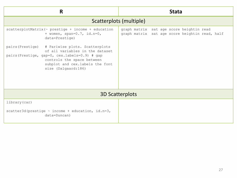
Scatterplots (multiple)scatterplotMatrix(~ prestige + income + education

+ women, span=0.7, id.n=0, data=Prestige)

pairs(Prestige) # Pariwise plots. Scatterplotsof all variables in the dataset

pairs(Prestige, gap=0, cex.labels=0.9) # gap controls the space between subplot and cex.labels the font size (Dalgaard:186)

graph matrix sat age score heightin readgraph matrix sat age score heightin read, half

3D Scatterplotslibrary(car)

scatter3d(prestige ~ income + education, id.n=3, data=Duncan)

27

R Stata

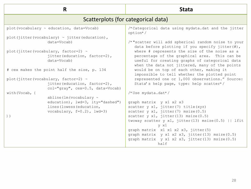
Scatterplots (for categorical data)plot(vocabulary ~ education, data=Vocab)

plot(jitter(vocabulary) ~ jitter(education), data=Vocab)

plot(jitter(vocabulary, factor=2) ~ jitter(education, factor=2), data=Vocab)

# cex makes the point half the size, p. 134

plot(jitter(vocabulary, factor=2) ~ jitter(education, factor=2), col="gray", cex=0.5, data=Vocab)

with(Vocab, {abline(lm(vocabulary ~ education), lwd=3, lty="dashed")lines(lowess(education, vocabulary, f=0.2), lwd=3)

})

/*Categorical data using mydata.dat and the jitter option*/

/*"scatter will add spherical random noise to your data before plotting if you specify jitter(#), where # represents the size of the noise as apercentage of the graphical area. This can be useful for creating graphs of categorical data when the data not jittered, many of the points would be on top of each other, making it impossible to tell whether the plotted point represented one or 1,000 observations.” Source: Stata’s help page, type: help scatter*/

/*Use mydata.dat*/

graph matrix y x1 x2 x3scatter y x1, jitter(7) title(xyz)scatter y x1, jitter(7) msize(0.5)scatter y x1, jitter(13) msize(0.5)twoway scatter y x1, jitter(13) msize(0.5) || lfit

y x1graph matrix x1 x1 x2 x3, jitter(5)graph matrix y x1 x2 x3, jitter(13) msize(0.5)graph matrix y x1 x2 x3, jitter(13) msize(0.5)

half

28

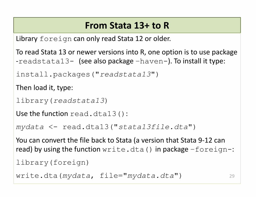
From Stata 13+ to RLibrary foreign can only read Stata 12 or older. 

To read Stata 13 or newer versions into R, one option is to use package ‐readstata13- (see also package –haven-). To install it type:

install.packages("readstata13")

Then load it, type:

library(readstata13)

Use the function read.dta13():

mydata <- read.dta13("stata13file.dta")

You can convert the file back to Stata (a version that Stata 9‐12 can read) by using the function write.dta() in package –foreign-:

library(foreign)

write.dta(mydata, file="mydata.dta") 29

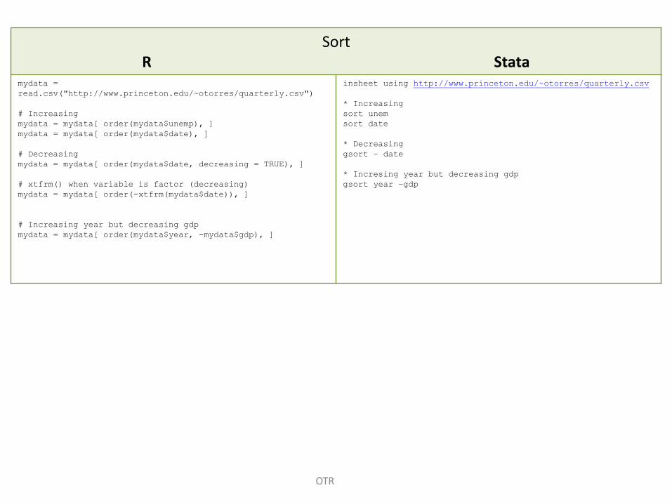
Sort R Stata

mydata =

read.csv("http://www.princeton.edu/~otorres/quarterly.csv")

# Increasing

mydata = mydata[ order(mydata$unemp), ]

mydata = mydata[ order(mydata$date), ]

# Decreasing

mydata = mydata[ order(mydata$date, decreasing = TRUE), ]

# xtfrm() when variable is factor (decreasing)

mydata = mydata[ order(-xtfrm(mydata$date)), ]

# Increasing year but decreasing gdp

mydata = mydata[ order(mydata$year, -mydata$gdp), ]

insheet using http://www.princeton.edu/~otorres/quarterly.csv

* Increasing

sort unem

sort date

* Decreasing

gsort – date

* Incresing year but decreasing gdp

gsort year –gdp

OTR

References/Useful links

• DSS Online Training Section http://dss.princeton.edu/training/

• Princeton DSS Libguides http://libguides.princeton.edu/dss

• John Fox’s site http://socserv.mcmaster.ca/jfox/

• Quick-R http://www.statmethods.net/

• UCLA Resources to learn and use R http://www.ats.ucla.edu/stat/R/

• UCLA Resources to learn and use Stata http://www.ats.ucla.edu/stat/stata/

• DSS - Stata http://dss/online_help/stats_packages/stata/

• DSS - R http://dss.princeton.edu/online_help/stats_packages/r

29

References/Recommended books

• An R Companion to Applied Regression, Second Edition / John Fox , Sanford Weisberg, Sage Publications, 2011

• Data Manipulation with R / Phil Spector, Springer, 2008

• Applied Econometrics with R / Christian Kleiber, Achim Zeileis, Springer, 2008

• Introductory Statistics with R / Peter Dalgaard, Springer, 2008

• Complex Surveys. A guide to Analysis Using R / Thomas Lumley, Wiley, 2010

• Applied Regression Analysis and Generalized Linear Models / John Fox, Sage, 2008

• R for Stata Users / Robert A. Muenchen, Joseph Hilbe, Springer, 2010

• Introduction to econometrics / James H. Stock, Mark W. Watson. 2nd ed., Boston: Pearson Addison Wesley, 2007.

• Data analysis using regression and multilevel/hierarchical models / Andrew Gelman, Jennifer Hill. Cambridge ; New York : Cambridge University Press, 2007.

• Econometric analysis / William H. Greene. 6th ed., Upper Saddle River, N.J. : Prentice Hall, 2008.

• Designing Social Inquiry: Scientific Inference in Qualitative Research / Gary King, Robert O. Keohane, Sidney Verba, Princeton University Press, 1994.

• Unifying Political Methodology: The Likelihood Theory of Statistical Inference / Gary King, Cambridge University Press, 1989

• Statistical Analysis: an interdisciplinary introduction to univariate & multivariate methods / Sam

Kachigan, New York : Radius Press, c1986

• Statistics with Stata (updated for version 9) / Lawrence Hamilton, Thomson Books/Cole, 2006

30