v.3

Notes on Elementary Probability and Statistics

RONY GOURAIGE

1

Preface

I have been teaching for nearly a decade an introductory probability and statistics course that

meets 3 hours per week for 14 weeks. These notes are based on my experience in teaching that

course, which has been a pedagogical challenge. On the one hand, most of my students are

relatively inexperienced in mathematics, having just completed a remedial course in elementary

algebra. On the other hand, for many of my students, this course will be the last mathematics

class that they will take. I want to give my students a taste of mathematics beyond just

computations, but I don’t want to overwhelm them with concepts for which they are unprepared.

I also want them to see the relevance of mathematical ideas to their lives. Probability and

statistics are ideally suited for these purposes. I have presented in these notes results that are

deep and beautiful, that may be explained to someone with little experience in mathematics, and

that are widely used to solve practical problems.

My comments above explain the two tracks in these notes. The lectures present the material

from a non-technical and, hopefully, intuitive viewpoint, while striving for the precision that is

expected of a mathematical theory. In the appendices, I give some of the basic mathematical

concepts that clarify, unify, and simplify some of the ideas that are discussed in informal terms

in the lectures. A perusal of the appendices will reveal that I have gone much further than what

is indicated in the preceding sentence. In particular, in Appendices A, C and F I have explored

some topics to a greater depth than is strictly necessary as background for the lectures. These

appendices are unsuitable for the typical student in my class. However, I have had some well-

prepared and enthusiastic students who would have enjoyed reading these appendices.

There are no innovations in these lectures. I cover some of the standard basic topics in the

standard way. So why did I write these notes? I had the following four goals:

1. I wanted to give my students an alternative to the very expensive textbooks in the market.

2. I wanted to give my students a short book that does not sacrifice clarity. I have tried to

write as clearly as my knowledge, experience, and ability to write permit. There are even

places where I may justly be accused of prolixity. I have achieved brevity by focusing on

what I believe to be the essential ideas needed for a sound introduction to probability

and statistical inference and unceremoniously ignoring everything else.

3. I wanted to write a book that is suitable for my students. There are many excellent books

on introductory probability and statistics, and I have learned a lot from these books, but

they are pitched at a level that is not suited to my students.

4. I wanted to write a book that someone who is interested in learning about probability

and statistics could use to study on their own. I may have fallen short of that goal. The

written word can never substitute for the dynamic interaction between an inquisitive

2

student and a competent teacher. Nevertheless, I hope that these notes may be of some

use to someone studying on their own.

Guide to Teachers The first thing to understand is that these notes cover fewer topics than other

textbooks that are written for a broader market. If you believe that introducing the basics of

experimental design or the visual presentation and analysis of large data sets are essential in an

introductory probability and statistics course, then this is not the textbook for you. These notes

focus on a narrow range of topics and give more weight to the probability than the statistics.

That is less a value judgment and more a reflection of my limited knowledge.

I have attempted to lay a sound foundation in the theory of probability to support the basics of

statistical inference presented in Lectures 11 and 12. The order of topics is necessarily rigid, and

I recommend covering the topics in the order given, although there is some flexibility in what to

emphasize. For example, it is quite workable (and I have done it many times) to go through the

material in Lectures 6, 7, and 10 lightly by only covering the fundamental principle of counting

and some of its basic applications in Lecture 6, going over only Example 7.1 (or another favorite

of your choice) in Lecture 7, and covering Theorem 10.1 and its applications thoroughly, but only

briefly discussing the Central Limit Theorem, in Lecture 10.

Finally, let me say something about the exercises. Practice problems are given as topics are

introduced to aid learning. At the end of each lecture are exercises that are intended to provide

the drill necessary to assimilate the material. Almost all of the exercises are straightforward. You

will have to provide more challenging problems, if that is what you like to do.

Guide to Students Read the lectures in the order given and refer to the appendices as needed

for background material or as your interest dictates. Do all the problems labelled Practice when

they appear. Do as many of the exercises at the end of the lectures as your time, stamina, and

interest allow. There are two sample exams at the end of these lectures to test yourself.

If you find a passage difficult, make sure that you understand clearly the meaning of the terms

being used. Also, study the surrounding examples carefully. If these suggestions don’t help, then

move on and come back to these difficult parts later.

These notes reflect the (hopefully uncontroversial) view that a rational approach to decision

making under conditions of uncertainty must be based on a sound mathematical theory of

probability. As a consequence, I emphasize the mathematical structure more than you are

probably accustomed to from your previous mathematics courses. Be patient, read slowly, think

critically, study the examples carefully, and solve plenty of problems. It will take time to

acclimate yourself to precise thinking and argument. Probability is a glorious and entertaining

subject, and statistical methods permeate our lives whether we are aware of it or not. This

material is both fun and useful. Learn it well.

Acknowledgments I have had an incomplete set of lecture notes for many years, always

intending to polish these for publication, but never finding the time to do so. The final impetus

3

to actually do it came when I saw the beautiful class notes of my student Jaileen Encarnacion.

She kindly gave these to me. The task of writing these lecture notes was made much easier after

that.

The following three excellent textbooks have shaped my approach to teaching probability and

statistics:

1. Bhattacharyya and Johnson, Statistical Concepts, John Wiley & Sons

2. Brase and Brase, Understanding Basic Statistics, 8th ed., Cengage Publishing

3. Wackerly, Mendenhall, and Scheaffer, Mathematical Statistics with Applications, 7th ed.,

Thomson Brooks/Cole

Obligatory Statement of Responsibility Any errors, omissions, and misleading or obscure

statements are my responsibility. I shall appreciate it if a reader who spots such infelicities would

kindly take the time to send me an e-mail at rony.gouraige@bcc.cuny.edu.

4

Table of Contents

Lecture 1: Basic Concepts and an Introduction to Statistical Inference

Lecture 2: Measures of Central Tendency

Lecture 3: Measures of Variation

Appendix A: Chebyshev’s Theorem

Lecture 4: Probability

Lecture 5: The Multiplication and Addition Laws

Appendix B: Set Theory

Appendix C: Probability Spaces

Lecture 6: Counting

Appendix D: Factorial Notation, Permutations, and Combinations

Lecture 7: Random Variables, Probability Distributions, and Expected Values

Appendix E: Functions and their Graphs

Lecture 8: Binomial Random Variables

Lecture 9: Normal Random Variables

Lecture 10: The Central Limit Theorem

Appendix F: Infinity

Lecture 11: Confidence Intervals

Lecture 12: Hypothesis Tests

Lecture 13: Scatter Diagrams and Correlation Coefficients

Finis

Sample Exams A and B

5

Lecture 1: Basic Concepts and an Introduction to Statistical Inference

Let us begin our study of probability and statistics with a simple example.

Example 1.1 There are about 8,000 students at Bronx Community College (BCC). What is the

average number of hours worked per week for these BCC students? It would be time consuming

and costly to collect the number of hours worked per week for all 8,000 students. Instead, a

random sample of 50 students is drawn, the average number of hours worked per week is

calculated for only these students, and it is 18.3. What does this average, which is based on only

a sample of size 50, tell us about the average for the entire population of 8,000 students? For

instance, does this sample result provide strong evidence that students at BCC work on average

more than 15 hours per week?

The preceding example is typical of the type of problem that we shall consider in this course.

Before we describe the general problem that we shall investigate, we need to introduce some

terminology.

Definitions 1.1

1. Population: The collection of all objects of interest in a particular study.

Comment: The population in Example 1.1 consists of 8,000 numbers, each representing

the hours worked per week of a student at BCC.

2. Sample: Some of the objects drawn from a population.

Comment: The sample in Example 1.1 consists of 50 numbers, each representing the

hours worked per week of one of the selected students.

3. Random Sample: A sample of size 𝑛 such that all groups of 𝑛 objects in the population

are equally likely to be selected. (See Remark 6.3 for a more precise definition.)

Comment: It is stated in Example 1.1 that the sample is random. One must be circumspect

about such claims and determine exactly how the sample was collected. See Example 1.2

and Remark 1.2 below.

4. Parameter: A numerical measure of some characteristic of a population.

Comment: The parameter in Example 1.1 is the average hours worked per week of all

8,000 students. It measures the center of all 8,000 numbers.

5. Statistic: A numerical measure of some characteristic of a sample.

Comment: The statistic in Example 1.1 is 18.3, the average of the 50 numbers in the

sample. It measures the center of the sample.

Remark 1.1 Everything that we do in this course will be based on the assumption that all samples

considered are random. Non-random samples do arise in practice, but we shall not consider

these in this course. It is helpful to keep the following principle in mind: If a sample is random,

6

then the general features of the sample should, roughly, reflect the general features of the

population from which it was drawn.

Let us try to get a feel for what is and is not a random sample.

Example 1.2 A club has 100 members, ten of whom are to be chosen and then interviewed. Is it

a random sample if the club members are asked to volunteer and the first 10 that do are

interviewed? No. Some people just will not volunteer and thus will never be selected by this

method.

Is it a random sample if we interview the 5 most senior members and the 5 most junior members?

No. This method appears to be an attempt to be fair, but random does not mean fair. This

method will never select the 10 most senior or the 10 most junior members. In other words,

using this method, some groups of 10 members will never be chosen.

Is it a random sample if each member is assigned a number, the numbers are written on index

cards, the index cards are thoroughly shuffled, and the members corresponding to the numbers

on the top 10 cards are interviewed? Yes! This mechanical procedure gives every group of 10

members the same chance of being chosen as any other group of 10.

Remark 1.2 Going back to Example 1.1, it is of course not feasible to randomly select 50 students

from 8,000 by the procedure described in Example 1.2. Fortunately, there are computer

programs and random number tables available that may be used to make such random selections

from a large population. If you are interested, you may find out about these methods by doing a

web search.

We may now state the fundamental problem that we shall consider in this course.

The Problem of Statistical Inference What may we infer about a population parameter based

only on the information obtained from a random sample?

It is important to understand that once a population has been identified, all parameters are

definite, fixed numbers. These population parameters may be unknown to us, but, in principle,

one may calculate them if complete information about the population was available. It is

generally impractical (or may even be impossible) to obtain complete information about a large

population, and so we rely on partial information contained in a random sample.

Unlike parameters, statistics vary unpredictably from sample to sample. It is hard to imagine

then that it would even be possible to come to any definite conclusions about an unknown

population parameter based solely on a sample statistic. Indeed, we will never be certain about

our conclusions, but we can make inferences and calculate in a precise way how reliable those

inferences are (see Remark 10.4). In order to do this, we need the theory of probability. We shall

study some basic probability theory in this course, but, for now, the following example will

indicate the fundamental role of probability in statistical inference. You may use whatever

intuitive understanding that you have of the word “probability” when reading the example.

7

Example 1.3 Ms. Rodriguez is running for election against one opponent in a large district with

several hundred thousand registered voters. A random sample of 100 registered voters is

chosen, and 62 indicate support for Ms. Rodriguez. Assuming, for simplicity, that all registered

voters will in fact vote, is it reasonable to conclude on the basis of this sample result that Ms.

Rodriguez has more than 50% support among registered voters and thus will likely win on

Election Day?

You may object that such a conclusion is unwarranted. For, is it not possible that Ms. Rodriguez

has only 50% support, but, because of pure chance, an unusually supportive group of registered

voters was selected? We cannot rule out that possibility, but how likely is it? In other words, if

Ms. Rodriguez enjoyed only 50% support, what is the probability of getting 62 or more supporters

among 100 randomly selected registered voters? Answer: About 1%. (We will see in Example

10.2 how this probability was calculated.)

One percent is a very low probability. Think about it this way: Would you carry an umbrella if the

forecast gave only a 1% chance of rain? There are two possibilities here: Either a rare event has

occurred or the assumption that Ms. Rodriguez has only 50% support is strongly contradicted by

the sample result. We shall adopt the latter view and conclude that on the basis of this sample

result, Ms. Rodriguez will likely win on Election Day.

Remark 1.3 There is an important principle in Example 1.3 that is worth stating explicitly: If an

assumption leads to a low (say, 5% or less) probability for an observed event, then that event is

strong evidence against the assumption. The idea is that the observed event is unlikely to have

occurred under the conditions contained in the assumption. Said another way, the observed

event cannot be explained by chance under the conditions stated in the assumption, and so it is

unlikely that those conditions prevail. Cf. Exercises 1.1-1.3 and Remark 10.4.

Exercise 1.1 Anna takes a multiple choice mathematics exam consisting of 20 questions. Each

question has four choices, and only one of these is the correct answer. Anna answers 18 of the

questions correctly. She is so proud of this result that she posts the exam on a social media

website. Almost instantly, her friend Mabel responds with the following comment: “You just got

lucky! I know that you are no good at math!” Disregarding the harshness of the comment, what

do you think about Mabel’s assertion that “luck” explains Anna’s result? Hint: If we assume that

Anna just randomly guesses answers, then the probability that she answers at least 18 questions

out of 20 correctly is, to three decimal places, .000 (that’s right: there are three zeros after the

decimal point). See Exercise 8.1.

Exercise 1.2 I insist that I can taste the difference between omelets made with generic versus

brand-name (meaning more expensive) liquid egg whites, but my wife is incredulous. We devised

a test. She served me 10 plain omelets that were randomly made using either generic or brand-

name egg whites. I tasted each omelet while blindfolded and determined which type of egg

whites was used. I correctly identified the type of egg whites used in 8 out of the 10 omelets.

Should my wife be convinced that I indeed can tell the difference between generic and brand-

8

name liquid egg white omelets? Hint: Suppose that I am in fact guessing. Then I have a 50%

chance of guessing correctly. What is the probability of getting at least 8 out of 10 correctly if I

was just guessing? You will find out how to compute such a probability later in the course (see

Exercise 8.1), but for now I will give you the answer. It is .055.

Exercise 1.3 A coin is tossed 20 times and lands heads 17 times. Can this outcome be explained

by the assumption that the coin is fair; i.e., that heads is as equally likely as tails? Hint: You may

use the fact that assuming the coin is fair, the probability of at least 17 heads in 20 tosses is .001.

See Exercise 8.1.

9

Lecture 2: Measures of Central Tendency

Example 2.1 A random sample of the weights, in pounds, of five newborns at Mercy Hospital

produced the following result: 9.2, 6.1, 5.8, 7.4, 7.8. How may we summarize these five numbers

with a single number?

A “measure of central tendency” or “measure of center” is a single number that gives the

“typical” or “central” value of a group of numbers. Such measures distill a, possibly very large,

collection of numbers into a single number. There are many measures of central tendency, but

we shall only be concerned with two: the mean and the median, which are defined as follows:

Definitions 2.1

1. Median: This is the middle value when the numbers in the sample are arranged in order

from smallest to largest. If the sample size is odd (that is, 1, 3, 5, 7, etc.), then there is

only one number in the middle and that is the median. If the sample size is even (that is,

2, 4, 6, 8, etc.), then there are two numbers in the middle and the median in that case is

the average of the two middle numbers.

2. Mean: The sum of all the numbers in the sample divided by the sample size.

Remark 2.1 The mean will be the most important measure of central tendency for our purposes

because it is widely used and has desirable theoretical properties. However, the median is also

commonly used, especially if the numbers vary widely; for example, income or home prices are

often summarized by giving the median. Note that the median is calculated only after the

numbers have been ordered. The most common error committed when calculating the median

is failing to first arrange the numbers in order of their size.

Solution to Example 2.1 To calculate the median, we first order the numbers from smallest to

largest: 5.8, 6.1, 7.4, 7.8, 9.2. The median is therefore 7.4. As for the mean, we add the numbers

and then divide the sum by the sample size, which in this case is five. We get:

Mean =9.2+6.1+5.8+7.4+7.8

5=

36.3

5= 7.26

Example 2.2 Find the median and mean of the following sample of annual salaries, in thousands

of dollars, at a law firm: 500, 45, 53, 95, 42, 60, 51, 58.

Solution to Example 2.2 Arrange the numbers in order of increasing size: 42, 45, 51, 53, 58, 60,

95, 500. Notice that there are two numbers, namely 53 and 58, in the middle because the sample

size, eight, is even. In this case the median is the average of these two middle numbers:

Median =53+58

2=

111

2= 55.5

To calculate the mean, we add the numbers and divide the sum by the sample size:

10

Mean = 42+45+51+53+58+60+95+500

8=

904

8= 113

Remark 2.2 Which is the better measure of the center of the sample in Example 2.2, the median

or the mean? The median is preferable here because there is one salary, the 500, that is much

larger than all the other salaries and it inflates the mean. The mean includes all the salaries, but

the median ignores extreme (either very large or very small) values since it only measures what

is going on in the middle.

Here is an amusing way of remembering the difference between the median and the mean: What

happens to the median and mean net worth of the riders of a bus after Jeff Bezos gets on the

bus? (Hint: By one estimate, Jeff Bezos, the founder and CEO of Amazon, has a net worth of $138

billion. You may assume that the other riders on the bus are Amazon warehouse employees.)

Practice 2.1 Find the median and mean of each of the following samples:

a. 7, 3, 2, 1, 7

b. 500, 750, 600, 500, 550

c. 0, 2, 6, 4, 0, 6

d. 2.1, 4.9, 1.0, 9.9, 7.1, 8.3, 3.8, 8.3, 1.2, 4.0

e. $14.99, $17.50, $14.95, $15.00, $25.99

f. 123, 148, 111, 97, 139

Notation 2.1 Recall that parameters are fixed once the population is determined, but statistics

vary randomly from sample to sample. So it is important to distinguish between the population

mean (a parameter) and a sample mean (a statistic). The notation that does so is given in the

following table:

Population Sample

Mean 𝜇 �̅�

The symbol 𝜇 (read: “mew”) is the lower-case Greek letter mu, and it corresponds to the Latin

letter 𝑚. The symbol �̅� is read: “𝑥 bar.” This notational scheme reflects a general principle: Greek

letters are used for population parameters and Latin letters are used for sample statistics.

We shall also have frequent occasion to form the sum of a collection of numbers. The symbol

∑ … is used in mathematics as an abbreviation for “the sum of all …” The symbol ∑, read:

“sigma,” is the upper-case Greek letter corresponding to the capital Latin letter 𝑆. Using this

notation, we may give a compact formula for the sample mean:

�̅� =∑ 𝑥

𝑛 ,

where 𝑛 denotes the sample size. Read ∑ 𝑥 as “the sum of all the numbers 𝑥,” with the

understanding that 𝑥 varies over all the numbers in the sample.

11

Remark 2.3 The formula for a population parameter may vary from the formula for the

corresponding sample statistic, but this will never be an issue for us. We shall only have to

calculate sample statistics. (See however Remark 7.2.2-7.2.3.)

Exercise 2.1 Find the median and mean of each of the following samples. In each case, determine

if one measure is to be preferred over the other and justify your answer.

a. 3, 75, 86, 93, 72

b. 10, 4, 16, 2, 18

c. 15.1, 17.3, 12.4, 14.0, 15.3

d. 12, 12, 11, 14, 70

Exercise 2.2 The following are the test scores for three students in a Physics class.

Exam I Exam II Exam III Exam IV Exam V

Ricardo 45 45 65 100 95

Lyndon 40 40 70 80 90

Maymunah 30 50 60 70 70

a. What measure of center (median or mean) for their five scores would each student

prefer?

b. Consider now another common measure of center called the mode, which is defined as

the number that occurs most often in the sample. Is there a student who would prefer

the mode over either the median or mean?

The moral of Exercise 2.2 is that there are many measures of central tendency, each with its own

strengths and weaknesses, so be wary when only one is being used and determine if it is the

appropriate measure to use.

12

Lecture 3: Measures of Variation

In the last lecture, we learned how to summarize a sample with a single number that gives the

center of the sample. However, the mean, which is the most important measure of center for

us, is not by itself sufficient to describe the sample. There is another attribute, the tendency for

the numbers in the sample to deviate from the mean, that must also be measured in order to get

a more complete picture of the sample. Let us look at an example.

Example 3.1 A supervisor decided to track the productivity of two employees, Anton and Barbara.

On five randomly selected weeks, the number of completed reports submitted by Anton and

Barbara was recorded. This information is summarized in the following table:

Anton 15 5 10 25 20

Barbara 10 20 20 10 15

Notice that the median and mean number of reports per week for both Anton and Barbara are

15 (verify this). As far as these measures of center are concerned, there is no distinction between

these two employees. However, there is a sense in which Barbara is a more consistent

performer: Her productivity shows less variation. It is this attribute that we wish to measure

numerically.

Remark 3.1 How do we measure the variation in a sample? Well, we first choose a measure of

center. For theoretical reasons that need not concern us, we choose the mean. Next, we shall

attempt to measure variation away from the mean in the most obvious way: We shall subtract

the mean from each number in the sample, and then calculate the average of these deviations

from the mean. Let us do so for Anton’s sample in Example 3.1.

Example 3.1 continued First attempt to measure variation: Average the deviations from the

mean.

𝑥 𝑥 − �̅� 15 0

5 −10

10 −5

25 10

20 5

The second column in the above table gives the deviations from the mean of each number in the

first column. For example, 5 is 10 units below the mean of 15 and so its deviation is −10; 20 is 5

units above the mean of 15 and so its deviation is 5. Now if we attempt to average the deviations,

13

a curious thing happens: The sum of the deviations is 0, and so the average deviation, our first

naïve attempt to measure variation, is 0.

What is going on here? Look at the deviations in the second column. Some are negative (because

the number is below the mean) and some are positive (because the number is above the mean).

The positive deviations are cancelled out by the negative deviations, and the result is that the

average deviation from the mean is 0. This always happens when we use the mean as the

measure of center. (Check what I have just written using the following sample: 1, 5, 2, 5. Can

you see why the sum of the deviations from the mean is always 0? In fact, the mean is the unique

number with this property. See Application F.1 in Appendix F.)

Remark 3.2 So our first attempt to measure variation away from the mean failed. But why did it

fail? Because the deviations cancel out. How may we avoid this cancellation? There are at least

two approaches: We could replace each deviation by its absolute value or we could replace each

deviation by its square. It turns out that the latter method has more desirable theoretical

properties, and so we adopt it. That is, we shall “average” the squares of the deviations from the

mean. Notice those quotation marks in the preceding sentence. The reason that I placed average

in quotes is that after summing the squared deviations, we shall divide not by the sample size,

but by one less than the sample size. Why? Because the sample statistic that we obtain by

dividing by one less than the sample size is a better (in a precise way which need not concern us)

estimator for the corresponding population parameter. Let us return to the computation of the

variation in Anton’s sample.

Example 3.1 continued We shall square each deviation from the mean, sum those squares, and

divide that sum by one less than the sample size to obtain what is called the variance of the

sample.

𝑥 𝑥 − �̅� (𝑥 − �̅�)2 15 0 0

5 −10 100

10 −5 25

25 10 100

20 5 25

Sum 250

Sample Variance =250

5−1=

250

4= 62.5

We now give the formal definition of the sample variance using the notation that we introduced

in Lecture 2.

Definition 3.1

Sample Variance:

14

Sample Variance = ∑(𝑥−�̅�)2

𝑛−1

where 𝑛 denotes the sample size.

Remark 3.3 I have gone into great detail to explain why the sample variance is defined the way

it is. The advantage of the defining formula is that it clearly displays exactly what is being

measured. However, it turns out that when one has to actually compute the sample variance,

another equivalent computation formula is often more convenient. (The equivalence is

established in Application F.2 in Appendix F, if you are interested.) We give this computation

formula, and then return to Anton’s sample and recalculate its variance using that computation

formula.

Computation Formula for the Sample Variance

Sample Variance =𝑛(∑ 𝑥2)−(∑ 𝑥)2

𝑛(𝑛−1)

where 𝑛 is the sample size.

Example 3.1 continued

𝑥 𝑥2 15 225

5 25

10 100

25 625

20 400 ∑ 𝑥 = 75 ∑ 𝑥2= 1375

Sample Variance =5(1375)−(75)2

5(5−1)=

6875−5625

20=

1250

20= 62.5

This result agrees with our earlier computation using the defining formula.

Important From now on, always use the computation formula to calculate the sample variance.

Practice 3.1 Compute the variance of Barbara’s sample. Is it smaller than the variance of Anton’s

sample?

Remark 3.4 We are not quite done with the problem of measuring variation in a sample. Notice

that the squaring that we introduced to avoid cancellations changes the units. For example, if

the original numbers in the sample are in pounds, then the variance will be in pounds squared.

This is easily remedied by taking the square root of the variance. This leads us to the following

definition.

15

Definition 3.2

Sample Standard Deviation: The sample standard deviation is the square root of the sample

variance:

Sample Standard Deviation = √Sample Variance

Convention For convenience, we shall always round the standard deviation to two decimal

places.

Example 3.1 continued The standard deviation of Anton’s sample, rounded to two decimal

places, is

Standard Deviation = √62.5 = 7.905 … ≈ 7.91

Practice 3.2 Compute the standard deviation, rounded to two decimal places, of Barbara’s

sample.

Remark 3.5 The standard deviation will be the most important measure of variation for us. The

mean and standard deviation provide very useful information about a sample. For more on this,

see Appendix A. Also, these two sample statistics will be the primary tools that we shall use, in

conjunction with the theory of probability, to make statistical inferences about the population

mean.

Notation 3.1 Just as with the mean, we shall want notation that distinguishes between the

population variance (or standard deviation) and the sample variance (or standard deviation). This

notation is summarized in the following table:

Population Sample

Mean 𝜇 �̅�

Variance 𝜎2 𝑠2 Standard Deviation 𝜎 𝑠

Remark 3.6 The symbol 𝜎 is the lower-case Greek letter sigma that corresponds to the lower-

case Latin letter s. As we observed earlier, the convention is to use Greek letters for population

parameters and Latin letters for the corresponding sample statistics. We may now summarize

the sample statistics that will be the basis of our study of statistical inference in this course.

Summary of Sample Statistics

�̅� =∑ 𝑥

𝑛

𝑠𝟐 =𝑛(∑ 𝑥2) − (∑ 𝑥)2

𝑛(𝑛 − 1)

16

𝑠 = √𝑠𝟐

Remark 3.7 You do not have to memorize these formulas. You will be given a table of formulas

for each exam. However, you do have to know how to use the formulas to calculate the statistics.

Exercise 3.1 Find the median, mean, variance, and standard deviation (rounded to two decimal

places) of each of the following samples.

a. 2, 0, 1, 2, 3

b. 4, 12, 14, 8, 10

c. 5, 6, 8, 10, 2, 2

d. 8, 2, 7, 2, 6, 5, 1, 1

e. 9.2, 6.4, 10.5, 8.1, 7.8, 1.2, 3.2

f. $15.20, $14.00, $15.00, $12.50, $14.50

g. 145, 132, 35, 225, 56

Exercise 3.2 Consider the following random sample of 40 waiting times, in minutes, to check out

for customers of Acme Hardware Store:

1.3 1.1 2.3 7.8 15.0 2.1 2.1 2.0 3.4 5.7

1.8 1.8 6.6 5.8 3.2 2.0 2.0 2.0 1.4 6.8

13.9 1.3 1.5 4.6 2.3 2.8 2.9 2.6 2.3 2.2

2.4 2.4 3.8 6.5 22.5 1.0 1.5 2.3 2.7 2.4

Given that ∑ 𝑥 = 160.1 and ∑ 𝑥2 = 1357.81, compute �̅�, 𝑠2, and 𝑠. The median is 2.35. Which

is a better measure of center for this sample, the median or the mean? Why?

Exercise 3.3 In this exercise, we have summarized the sample in Exercise 3.2 in the form of a table

(see Table 3.1), called a relative frequency table. Notice that the sample is partitioned into eight

classes (that is, each number in the sample lies in exactly one class). Each class is an interval of

length 2.7. The relative frequency of a class is the frequency of that class (meaning how many

numbers in the sample lie in that class) divided by the sample size.

17

Class Frequency Relative

Frequency

1.0 - 3.7 29 .725

3.8 - 6.5 5 .125

6.6 - 9.3 3 .075

9.4 - 12.1 0 .000

12.2 - 14.9 1 .025

15.0 - 17.7 1 .025

7.8 - 20.5 0 .000

20.6 - 23.3 1 .025

Table 3.1

(Don’t worry about how this table was produced. Although I prepared it, there are statistical

programs that quickly produce such tables and are capable of handling much larger samples.)

a. What is the sum of the frequencies in the second column? Explain.

b. What is the sum of the relative frequencies in the third column? Explain.

c. Interpret the relative frequency of a class as the probability that a randomly chosen

number from the sample lies in that class. Notice that each probability is a number

between 0 and 1 and that the sum of all the probabilities is 1. If a number is randomly

chosen from the sample, what is the probability that it lies between 6.6 and 14.9? What

is the probability that it lies outside the interval from 6.6 to 14.9? Do you notice a

relationship between these two probabilities? Explain.

Remark on Exercise 3.3 It is helpful to have a visual representation, that is, a graph, of the data

given in the table in Exercise 3.3. There are two types of graphs that one may draw. One is called

a frequency histogram. There are statistics programs that produce frequency histograms. I used

Microsoft Excel to draw the following frequency histogram (Figure 3.1). The rectangles are

centered over the midpoints of each class interval.

18

Figure 3.1

We describe this type of frequency histogram as skewed right because of the tail that extends to

the right. Can you think of other data that may show such a pattern? Hint: What about waiting

time, in minutes, before a customer service agent is available to respond to your phone call?

Another type of graph is called a relative frequency histogram. See Figure 3.2. It differs from

the frequency histogram in that the rectangles are drawn so that their areas give the relative

frequency of each class. That is to say, each bar in a relative frequency histogram has area equal

to the probability of the class interval over which it lies. Hence, in a relative frequency histogram,

probability is given by areas in the histogram. Cf. the discussion of continuous random variables

and probability density curves in Lecture 9.

Figure 3.2

0

5

10

15

20

25

30

35

2.35 5.15 7.95 10.75 13.55 16.35 19.15 21.95

Frequency

0

0.1

0.2

0.3

0.4

0.5

0.6

0.7

0.8

2.35 5.15 7.95 10.75 13.55 16.35 19.15 21.95

Relative Frequency

19

Appendix A: Chebyshev’s Theorem

We have introduced the mean as a measure of center and the standard deviation as a measure

of variation. These two numbers summarize a collection of numbers that may be very large. We

pose the question: To what extent does the mean and standard deviation of a sample

characterize the distribution of the numbers in the original sample? By “distribution” is meant

the relative frequency of the numbers in the sample that lie between two given numbers (cf.

Exercise 3.3, which you should do now if you have not already done so). It is remarkable that

one may draw definite conclusions about the distribution of the numbers in the sample after

these have been distilled to only the mean and standard deviation. This is the essence of

Chebyshev’s Theorem.

Theorem A.1 (Chebyshev’s Theorem) If a sample has mean �̅� and standard deviation 𝑠, then for

any number 𝑘 > 1, the relative frequency of the numbers that lie between �̅� − 𝑘𝑠 and �̅� + 𝑘𝑠 is

at least 1 − 1 𝑘2⁄ .

Remark A.1 Chebyshev’s Theorem is telling us the minimum relative frequency that we may

expect to find for an interval generated by starting at the mean (roughly, the center) of the

sample and moving 𝑘 standard deviations (roughly, the spread away from the center) below and

above the mean.

There is a nice probabilistic interpretation of Chebyshev’s Theorem. If we randomly draw a

number from a given sample with mean �̅� and standard deviation 𝑠, then for any number 𝑘 > 1,

the probability that that number lies between �̅� − 𝑘𝑠 and �̅� + 𝑘𝑠 is at least 1 − 1 𝑘2⁄ . Note that

in this interpretation, probability is relative frequency, an idea that we shall return to later in our

discussion of probability theory.

Example A.1 Suppose that a random sample has mean 12.1 and standard deviation 2.94. Then

at least 75% of the numbers in the sample lie between 6.22 and 17.98 using 𝑘 = 2 in Chebyshev’s

Theorem. At least 88.9% lie between 3.28 and 20.92 using 𝑘 = 3 in Chebyshev’s Theorem. At

least 93.75% lie between 0.34 and 23.86 using 𝑘 = 4 in Chebyshev’s Theorem.

Remark A.2 Chebyshev’s Theorem is mostly of theoretical interest, and we shall not make any

use of it again. However, it is worth noting that in almost all samples, the actual relative

frequencies are much larger than the minimums guaranteed by Chebyshev’s Theorem. This is

particularly the case for samples in which the numbers are symmetrically situated about the

mean, as the following example shows. (Cf. The Empirical Rule following Remark 9.1.)

Example A.2 Consider Anton’s sample in Example 3.1. The mean is 15 and the standard deviation

is 7.91. Chebyshev’s Theorem (using 𝑘 = 1.2) guarantees that at least 31% of the numbers lie

between 5.508 and 24.492. In fact, 60% lie between those two numbers.

Practice A.1 Do the same for Barbara’s sample in Example 3.1.

20

Remark A.3 The preceding example is typical. Chebyshev’s Theorem guarantees a theoretical

minimum which in practice is far less than what one observes. This does not diminish the

usefulness of the result for theoretical considerations. Quite the contrary, the strength of

Chebyshev’s Theorem is its extreme generality since absolutely no restriction whatsoever is

placed on the nature of the sample. In a practical situation, Chebyshev’s Theorem may be used

to quickly estimate some relative frequencies and give a rough picture of a sample without

knowing the actual numbers in the sample. For our purposes, Chebyshev’s Theorem just gives

us some theoretical reassurance that the mean and standard deviation do indeed provide a good

description of the sample.

Exercise A.1 Consider the sample in Exercise 3.2. Compare the minimum relative frequency given

by Chebyshev’s Theorem for 𝑘 = 2 to the actual relative frequency in the sample.

Exercise A.2 Jorge has kept track of the times, in minutes, that it takes him to get to work in the

morning. The mean time is 63, and the standard deviation is 2.6. Estimate the probability that

Jorge’s commuting time on any randomly chosen day will lie between 50 and 76 minutes. Hint:

Use Chebyshev’s Theorem with 𝑘 = 5.

Remark A.4 What is a “theorem”? It is a statement that has been proved. I shall now present a

proof of Chebyshev’s Theorem. Please do not be discouraged if you are unable to understand

the proof at first. You may have to read it several times before the ideas sink in. It is helpful to

apply the argument in the proof to an actual sample to see what is going on. For that purpose,

try using Anton’s sample in Example 3.1 and take 𝑘 = 1.2.

Proof of Chebyshev’s Theorem Suppose that 𝑘 > 1, and suppose that the sample has 𝑛 ≥ 2

numbers, of which 𝑚 of these numbers lie outside the interval from �̅� − 𝑘𝑠 to �̅� + 𝑘𝑠. If 𝑥 is one

of these outlying numbers, then since the distance from 𝑥 to �̅� is greater than 𝑘𝑠, if follows that

the square of that distance is greater than the square of 𝑘𝑠. That is to say, for each outlier 𝑥,

(𝑥 − �̅�)2 > 𝑘2𝑠2 (1)

The defining formula for 𝑠2 gives

𝑠2 =∑(𝑥−�̅�)2

𝑛−1≥

∑ (𝑥−�̅�)2′

𝑛−1>

𝑚

𝑛𝑘2𝑠2 (2)

where the prime in the second sigma signals that we are summing over only the outliers. The

first inequality in (2) follows because the number of outliers cannot exceed the sample size. The

second inequality in (2) follows from the inequality (1) and the fact that the denominator was

increased from 𝑛 − 1 to 𝑛. It follows upon division by 𝑘2𝑠2 that the relative frequency, 𝑚 𝑛⁄ , of

the numbers in the sample that are outliers is at most 1 𝑘2⁄ . Hence the relative frequency of the

numbers in the sample that lie inside the interval from �̅� − 𝑘𝑠 to �̅� + 𝑘𝑠 is at least 1 − 1 𝑘2⁄ . The

last statement is precisely the conclusion of Chebyshev’s Theorem. QED

21

Lecture 4: Probability

Probability theory is ubiquitous in modern society. Casinos and insurance companies rely on

probability theory to operate profitably. Physicists use probability theory to describe nature at

its most fundamental level. Pharmaceutical companies use probability theory to determine if a

new drug is better than an existing drug. Engineers use probability theory to model

communication over a noisy channel. A manufacturer uses probability theory to determine if a

lot of parts has met quality standards and is ready to ship. Investment banks use probability

theory to make investment decisions. More mundanely, each of us has had occasion to check

the weather forecast, which relies on probability theory, before deciding what to wear on a given

day. The list goes on and on.

As natural as probability may appear to us today, it may be difficult to conceive of a time when

this was not so. However, for thousands of years, humans believed that nothing could be said

about the future, which was perceived to be inherently uncertain and unpredictable. The future

was best left to whatever deities were believed to exist at the time. There were some attempts

to take a rational approach to dealing with uncertainty, but the year 1654 marks a watershed in

human understanding of uncertainty. For in that year, a French nobleman and avid gambler by

the name of Chevalier de Mere pondered a problem, called the “problem of the points,” that had

baffled gamblers and mathematicians for nearly 200 years. Let me give you a very simple form

of the problem.

Simple Case of the Problem of the Points Suppose that two gamblers each put up $50 as a wager

on the following game. A fair coin will be tossed five times. One gambler chooses heads and the

other chooses tails. The gambler whose chosen face occurs three times among the five tosses

wins the game and collects the entire pot of $100 that was wagered. The problem of the points

is this: If, after three tosses, the game is interrupted and cannot be completed, then how should

the $100 pot be divided between the two gamblers?

De Mere could make no progress on the general problem, which is more complicated than the

simple version given above, and so in the summer of 1654, he proposed it to his friend, Blaise

Pascal, a brilliant French mathematician. Pascal was intrigued by this problem, and he wrote a

letter describing it to his friend and mentor, Pierre de Fermat, another outstanding French

mathematician. (It is interesting to note that Fermat, one of the finest mathematicians ever, was

a lawyer and judge who studied mathematics for the sheer pleasure of it.)

Over the course of several months in 1654, Pascal and Fermat exchanged correspondence and

laid the foundations of the modern theory of probability while solving the problem of the points.

If you are interested in learning more about this fascinating story, then take a look at Keith

Devlin’s book with the enticing title The Unfinished Game: Pascal, Fermat, and the Seventeenth-

Century Letter that Made the World Modern.

The theory of probability continued to be developed by its adherents after the momentous

events of the summer of 1654, but the theory was looked upon with some skepticism by the

22

mathematical community because it failed to meet the high standards of rigor expected of a

mathematical theory. That skepticism was addressed in 1933 when the great Soviet

mathematician Andrey Kolmogorov promulgated the axioms for a theory of probability that are

generally used today. The approach that we shall take in these notes is based on Kolmogorov’s

axioms. (See Appendix C for a more formal presentation of Kolmogorov’s axioms.)

As we have seen, probability has its roots in the analysis of games of chance. We shall therefore

begin our study of probability with a simple game of chance. When we have the basic concepts

available, we shall return to the simple case of the problem of the points described above and

solve it (see Example 4.2).

Disclaimer Please do not infer from my enthusiasm for probability that I advocate gambling.

Quite the opposite, based on my understanding of the theory of probability, my advice is not to

gamble because the odds are never in your favor.

Example 4.1 The basic ingredients for a theory of probability are a random experiment, its

associated sample space, a collection of events of interest, and an assignment of probability to

each of these events. We shall elaborate on these concepts by considering the roll of a balanced

die.

Random Experiment A balanced die is rolled, and the number of dots on the top face is recorded.

What is random about this activity? Anybody who has ever played a game involving the roll of a

die knows very well what the problem is: We cannot predict with certainty which face will land

on top. What can we do? For thousands of years the answer was to appeal to the gods for good

fortune. Vestiges of that approach still exist today, for example, when the gambler, before rolling

a die, exclaims “Luck be a lady tonight!” The modern theory of probability, however, offers an

alternative.

Sample Space We may not be able to predict which face will land on top, but we do know the

possible outcomes when we roll the die. The collection of all the possible outcomes to a random

experiment is called its sample space, and we shall denote it by the letter 𝑆. Using set notation

(refer to Appendix B if you are unfamiliar with this notation), the sample space for our die rolling

experiment is

𝑆 = {1, 2, 3, 4, 5, 6}

because these are the only possible outcomes for the number of dots on the top face.

Events Associated to any random experiment are certain events that are of interest to us. For

example, we may be interested in the following events:

A: the number rolled is even

B: the number rolled is at least 3

C: the number rolled is at most 5

23

We may also describe these events, just as we did with the sample space, more compactly by

using set notation:

𝐴 = {2, 4, 6}

𝐵 = {3, 4, 5, 6}

𝐶 = {1, 2, 3, 4, 5}

In this form, we see that an event is just a collection of outcomes, that is, a subset of the sample

space. Each time the die is rolled, we may ask: Did a certain event of interest occur? An event is

said to occur if the outcome of the experiment is one of the outcomes in the event. For example,

if the die lands with a 1 on top, then 𝐶 occurred, but 𝐴 and 𝐵 did not.

It is useful to have a term for the case in which an event does not occur. We say the complement

of an event occurs if the event does not occur. We indicate the complement of an event by

affixing a superscript “c” to the label for the event. For example, for the events A, B, and C given

above, their complements are:

𝐴𝑐 = {1, 3, 5}

𝐵𝑐 = {1, 2}

𝐶𝑐 = {6}

Notice that the complement consists of all the outcomes in the sample space that are not in the

event. For example, if the die is rolled and 2 lands on top, then A and 𝐶 occurred, but B did not,

and so 𝐵𝑐 occurred. In other words, after each performance (we also say trial) of the experiment,

we can ask if an event of interest occurred. If the answer is “Yes,” then, of course, the event

occurred, but if the answer is “No,” then the complement of that event occurred. Remember

this: In any trial of the random experiment, for any given event, either the event or its

complement, but not both, must occur.

Practice 4.1

a. Use set notation to describe the event D: the number rolled is more than 4. Do the same

for 𝐷𝑐.

b. If the die is rolled and 6 lands on top, which of the events D and 𝐷𝑐 occurred? What if 4

lands on top?

c. Intuitively, which is more likely to happen, D or 𝐷𝑐? Explain your choice.

Practice 4.2 The sample space, being a collection of outcomes, is an event. What is its

complement? Hint: There is an empty collection of outcomes, denoted by the symbol ∅. See

Appendix B.

Assignment of Probability There is uncertainty about the outcome of the roll of a balanced die.

We now want to assign a number to each outcome that measures the likelihood that it will occur.

24

That number is called the probability of the outcome. What should we require of this

probability? We are guided by the notion of relative frequency that was introduced in Exercise

3.3. (Do that exercise if you have not already done it.) The first requirement is that probability

should be a number between 0 and 1. The closer the probability is to 1, the more likely is the

outcome to occur. The closer the probability is to 0, the less likely is the outcome to occur. If an

outcome has probability 1, then it is certain to occur. If an outcome has probability 0, then it is

certain not to occur. The second requirement that we shall insist on is that the sum of the

probabilities of all the outcomes is 1. This second requirement makes sense intuitively since at

least one outcome must certainly occur each time the experiment is performed.

In the random experiment under consideration, there is really only one rational assignment of

probability: Each face is equally likely to land on top as any other face (that is what is meant by a

“balanced” die) and there are six faces, so each outcome should be assigned probability 1 6⁄ .

More generally, how do we assign probabilities to events consisting of more than one outcome?

Easy: Just add up the probabilities of the outcomes in the event. In other words, the probability

of an event E, denoted P(E) (read: “probability of E”), is the ratio:

𝑃(𝐸) =Number of Outcomes in 𝐸

Number of Outcomes in 𝑆=

Number of Outcomes in 𝐸

6

because there are only six outcomes in the random experiment that we are considering. Notice

that if E consists of only one outcome, then we recover the probability 1 6⁄ that we arrived at

before.

Let us compute the probabilities of some of the other events considered above:

𝑃(𝐴) =3

6=

1

2= .5 = 50%

𝑃(𝐵) =4

6=

2

3≈ .67 = 67%

𝑃(𝐶) =5

6≈ .83 = 83%

Notice that a probability may be expressed in several equivalent ways, depending on

convenience or custom.

Practice 4.2 Calculate the probabilities of 𝐴𝑐, 𝐵𝑐, and 𝐶𝑐. Do you notice any relationship between

the probability of an event and the probability of its complement?

Practice 4.3 Referring to Practice 4.1, what are the probabilities of D and 𝐷𝑐? Does the event

that you intuitively believed to be more likely have the higher probability? What do you get when

you add these two probabilities? Compare with Practice 4.2.

25

Remark 4.1 We have discussed the random experiment of rolling a balanced die in great detail

because it is simple, but not completely trivial. Let us now formulate the concepts introduced in

that example in greater generality. It will be helpful, as we make the following general

definitions, to keep the example of rolling a balanced die in mind.

Definitions 4.1

1. Random Experiment: Any activity or observation that results in a definite, but

unpredictable, outcome.

2. Sample Space: The collection of all the outcomes to a random experiment.

3. Event: Any collection of outcomes to a random experiment.

4. Complement of an Event: The event does not occur. That is, the collection of outcomes

that are not in the event.

5. Assignment of Probability: Each event is assigned a number between 0 and 1, called its

probability, that measures the likelihood that the event will occur before the random

experiment is performed. In the case of a random experiment with only a finite number

of outcomes, the assignment of probability is determined by giving the probabilities of

each outcome subject to the following requirements:

a. For any outcome 𝐸, 0 ≤ 𝑃(𝐸) ≤ 1

b. ∑ 𝑃(𝐸) = 1, where the sum is over all the outcomes of the random experiment

Assigning Probabilities in Practice The mathematical theory of probability does not specify how

probabilities are to be assigned. In a practical situation, however, there are generally two

methods employed to assign probabilities:

a. Equally Likely Outcomes If there is no reason (based either on logical or physical

grounds) to believe that any one outcome is more likely to occur than any other (all

the outcomes are equally likely), then the probability of an event associated to that

random experiment is the number of outcomes in that event divided by the total

number of outcomes in the sample space. This method is used to assign probabilities

in games of chance with equally likely outcomes. Intuitively, these probabilities

should approximate the relative frequency of that event when the random

experiment is repeated a large number of times.

b. Relative Frequency The probability of an event is the relative frequency with which it

occurs in a sample. That is, the probability of an event is the number of times that it

occurs in the sample divided by the sample size. This method is used when a sample,

for example, a survey or poll, is the basis for the assignment of probabilities.

26

Interpretation of Probability Intuitively, the probability of an event is its long-term relative

frequency. That is, if the experiment is repeated many, many times, then the fraction of the times

that the event occurs will approximate its probability. (See Theorem F.6 for a precise statement.)

Thus, if a fair coin is tossed thousands of times, we expect that the fraction of times that it lands

heads will be near 1 2⁄ . This is the so-called frequentist interpretation of probability.

There is another competing interpretation of probability as a “measure of the degree of belief,”

but we shall not discuss this because I am not qualified to enter into a philosophical debate over

what probability actually is. Such debates have value, but the mathematical theory of probability

that we shall develop does not depend on any particular interpretation of probability, and that

is one of the strengths of the theory. (See Remark C.2 for more on this, if you are interested.)

Remark 4.2 You may have already noticed (cf. Practice 4.2 and 4.3) that there is a relationship

between the probability of an event and the probability of its complement: The sum of these

probabilities is 1. This is a general result that always holds and is our first law of probability,

which we state explicitly as:

The Law of the Complement If A is any event, then

𝑃(𝐴) + 𝑃(𝐴𝑐) = 1

Remark 4.3 See Appendix C if you are interested in a proof of this law. One application of this

law occurs when we want to calculate the probability of an event, but it is easier to calculate the

probability of its complement. In that case, we may apply the law of the complement to calculate

the probability of the event by subtracting the probability of its complement from 1. (See

Exercises D.2 and D.3 for applications of this idea.)

Practice 4.4 In a random experiment, the event 𝐴𝑐 has probability .23. What is the probability of

the event A?

Practice 4.5 A balanced die is rolled 10 times in succession. What is the probability of rolling a 4

at least once? Hint: The probability of not a rolling a 4 is 16%. See Exercise 8.2.

Example 4.2 (Solution to the Simple Case of the Problem of the Points) Recall the problem of

the points that initiated our study of probability. The game is interrupted after three tosses. Let

us assume for the sake of definiteness that heads (denoted by H) occurred twice and tails

(denoted by T) occurred once in the three tosses. In how many ways could the game be finished?

There are two more tosses remaining, and thus there are four possible outcomes for the

remaining tosses: HH, HT, TH, and TT. All of these outcomes are equally likely because the coin

is fair. The player who chose heads wins in three of these four outcomes. So the player who

chose heads should get 75% of the pot and the player who chose tails should get 25%.

Remark 4.4 We have illustrated the method of equally likely outcomes for assigning probabilities

in our discussion of rolling a balanced die and in the preceding example. The following example

illustrates the method of relative frequency.

27

Example 4.3 A survey of employees of a company is summarized in the following table.

Democrat (D) Republican (R) Independent (I) Row Totals

Executive (E) 5 34 9 48

Worker (W) 63 21 27 111

Column Totals 68 55 36 159

a. What is the probability that a randomly selected employee is an executive? We use the

method of relative frequency. There are 48 executives among the 159 employees. Hence

𝑃(𝐸) =48

159

b. What is the probability that a randomly selected employee is a Republican? There are 55

Republicans among the 159 employees. Hence

𝑃(𝑅) =55

159

c. What is the probability that a randomly selected employee is an executive and a

Democrat? Among the 159 employees, only 5 are both an executive and a Democrat.

Hence

𝑃(𝐸 and 𝐷) =5

159

d. What is the probability that a randomly selected employee is either a worker or a

Republican? There is some ambiguity in the use of the word “or” in the English language.

Sometimes it is used in the exclusive sense of either one or the other, but not both. For

example, when your teacher says “either pass the course or you will have to take it again,”

you naturally expect that only one of the two alternatives will occur.

Sometimes the word “or” is used in an inclusive sense. For example, if a curriculum

guideline states that a student may either take Physics 35 or Chemistry 32 to satisfy their

science requirement, then one believes that this allows the student to take both science

courses.

In order to avoid any confusion, in mathematics the word “or” is always used in the

inclusive sense of one or the other or both. Hence

28

𝑃(𝑊 or 𝑅) =111 + 55 − 21

159=

145

159

Notice the subtraction of the number 21. This is necessary to avoid “double counting.”

When we counted the 111 workers and then added to that number the 55 Republicans,

we counted the 21 workers that were also Republicans twice. Subtracting 21 corrects for

that double count.

e. What is the probability that the employee is a Democrat, given that the employee is a

worker? Notice here that we have been given some additional information, namely that

the employee must be a worker. What do we do with that information? We only consider

the workers; that is, the sample size is reduced from 159 to 111, the number of workers.

Hence

𝑃(𝐷, given 𝑊) =63

111

Notice that the denominator changed to reflect the given information. Notice also that

the numerator only reflects the Democrats that are workers. A common mistake is to put

68 in the numerator, but that ignores the information that we have been given. Once we

have been given that the chosen employee is a worker, we focus only on the workers and

ignore everybody else.

Practice 4.6 Use the survey results in the preceding example to calculate the following

probabilities:

a. 𝑃(𝑊)

b. 𝑃(𝐼)

c. 𝑃(𝑊 and 𝑅)

d. 𝑃(𝐸 or 𝐼)

e. 𝑃(𝐸, given 𝐼)

Exercise 4.1 A fair coin is tossed twice in succession and the face, either heads (H) or tails (T), that

lands on top is observed. Interpret “fair” to mean that heads is as equally likely to land on top as

tails.

a. What is the sample space in this random experiment?

b. What probability should be assigned to each outcome in the sample space? Hint: Use the

method of equally likely outcomes.

c. Use set notation to describe the event A: the number of heads in the two tosses is 1, and

then find P(A). Do the same for 𝐴𝑐.

d. Use set notation to describe the event B: the number of heads is at most 1, and then find

P(B). Do the same for 𝐵𝑐.

29

Exercise 4.2 The following table summarizes the results of a survey of registered voters.

Approve (A) Disapprove (D) Neutral (N) Row Totals

Male (M) 7 56 3 66

Female (F) 35 8 2 45

Column Totals 42 64 5 111

Find the following probabilities if a respondent is randomly selected:

a. P(M)

b. P(A)

c. P(M and A)

d. P(A, given M)

e. P(M or A)

Verify the following equalities:

f. 𝑃(𝑀 and 𝐴) = 𝑃(𝑀) ∙ 𝑃(𝐴, given 𝑀)

g. 𝑃(𝑀 or 𝐴) = 𝑃(𝑀) + 𝑃(𝐴) − 𝑃(𝑀 and 𝐴)

Exercise 4.3 Use the following table to compute the given probabilities.

Elementary School (E)

High School (H)

College (C) Graduate School (G)

Row Totals

Full-Time (FT)

25 72 98 131 326

Part-Time (PT)

47 56 62 83 248

Unemployed (U)

154 128 33 16 331

Column Totals

226 256 193 230 905

a. P(U)

b. P(H)

c. P(FT, given H)

d. P(C, given U)

e. P(U and G)

f. P(FT or E)

Exercise 4.4 In any random experiment, what is the probability of the sample space 𝑆? What is

the probability of the empty set ∅?

30

Exercise 4.5 Use the following table to compute the given probabilities.

Mild Moderate Severe Row Totals

Adult 13 32 10 55

Child 24 8 3 35

Column Totals 37 40 13 90

a. P(Adult)

b. P(Severe)

c. P(Child and Moderate)

d. P(Severe, given Adult)

e. P(Child or Moderate)

31

Lecture 5: The Multiplication and Addition Laws

We saw at the end of the last lecture (cf. Example 4.3) that while discussing probabilities based

on a survey, it is natural to ask about the probability that two given events occur simultaneously

or that at least one of these given events occurs. With the survey data available, it was easy to

calculate these probabilities by counting. But what if we don’t have the survey data? How do

we calculate probabilities of combinations of given events when all we have are the probabilities

of those given events? We address this question now.

Definition 5.1 Let 𝐴 and 𝐵 be events associated with a random experiment. We may form from

these given events new events, as follows.

1. A and B: The event A and B occurs when both 𝐴 and 𝐵 occur simultaneously.

2. A or B: The event A or B occurs if at least one, possibly both, of the events 𝐴 and 𝐵 occurs.

Example 5.1 Consider the die rolling example from Lecture 4 and the events

𝑈: 𝑟𝑜𝑙𝑙 𝑎𝑡 𝑚𝑜𝑠𝑡 4

𝑉: 𝑟𝑜𝑙𝑙 𝑎𝑛 𝑜𝑑𝑑 𝑛𝑢𝑚𝑏𝑒𝑟

Then the event 𝑈 and 𝑉 is roll an odd number that is at most 4. The event 𝑈 or 𝑉 is roll either an

odd number or a number that is at most 4 or both. Using set notation, we have

𝑈 = {1, 2, 3, 4}

𝑉 = {1, 3, 5}

𝑈 and 𝑉 = {1, 3}

𝑈 or 𝑉 = {1, 2, 3, 4, 5}

Remark 5.1 We want now to introduce the concept of conditional probability. It sometimes

happens that we are given (or we may assume as given) additional information that may be used

when computing probabilities. The probabilities that reflect this additional information are called

conditional. Before stating the formal definition, let us first consider the following simple

examples.

Example 5.2 Roughly half the population is female. Thus the unconditional probability that a

randomly chosen person is female is 50%. However, what if we are given the additional

information that the person chosen is pregnant? Does that change the probability that the

person is a female? Yes! The conditional probability that a randomly chosen person is a female,

given the additional information that that person is pregnant, is 100%.

Example 5.3 We just saw that additional information may drastically alter probabilities, but this

is not always the case. The unconditional probability of rolling either 1 or 3 with a balanced die

is 1 3⁄ . What if before we observe the outcome of the roll, we are told that the number rolled is

either 3, 4, or 5? Does that additional information change the probability that the number rolled

32

was either 1 or 3? No. Indeed, the additional information cuts down the sample space to {3, 4,

5}, but with respect to this new sample space, the probability of rolling either a 1 or 3 is still 1 3⁄ .

Definition 5.2 Conditional Probability: Let 𝐴 and 𝐵 be events associated with a random

experiment. The conditional probability of 𝐴, given 𝐵, denoted 𝑃(𝐴 ∣ 𝐵), is the probability that

the event 𝐴 occurs, given that the event 𝐵 has already occurred.

Remark 5.2 Do not confuse 𝑃(𝐴 and 𝐵) with 𝑃( 𝐴 ∣ 𝐵 ). These are different, as the following

example shows.

Example 5.4 Refer back to Example 5.1. We have

𝑃(𝑈) =2

3

𝑃(𝑉) =1

2

𝑃( 𝑉 ∣ 𝑈 ) =1

2

𝑃(𝑈 and 𝑉) = 1

3= 𝑃(𝑈) ∙ 𝑃(𝑉 ∣ 𝑈)

𝑃(𝑈 or 𝑉) =5

6= 𝑃(𝑈) + 𝑃(𝑉) − 𝑃(𝑈 and 𝑉)

Practice 5.1 Find 𝑃( 𝑈 ∣ 𝑉 ). Notice that 𝑃( 𝑈 ∣ 𝑉 ) ≠ 𝑃( 𝑉 ∣ 𝑈 ).

Example 5.4 illustrates the multiplication and addition laws for probability. We state these

explicitly as:

The Multiplication Law For any events 𝐴 and 𝐵,

𝑃(𝐴 and 𝐵) = 𝑃(𝐴) ∙ 𝑃(𝐵 ∣ 𝐴)

The Addition Law For any events 𝐴 and 𝐵,

𝑃(𝐴 or 𝐵) = 𝑃(𝐴) + 𝑃(𝐵) − 𝑃(𝐴 𝑎𝑛𝑑 𝐵)

Remark 5.2 The proofs of these laws may be found in Appendix C. However, the intuition behind

each one is simple enough. Consider first the multiplication law. Suppose that you want to find

out how many students in a class are both female and a math major. You could do this two ways.

One way is to ask all the female math majors in the class to stand up and count them. That way

corresponds to the left-hand side of the multiplication law. Another way is to first ask all the

females to stand up, and then ask those females who are math majors to remain standing while

the other females sit down. The females who remain standing constitute all the female math

majors in the class. The second way corresponds to the right-hand side of the multiplication law.

33

The intuition behind the addition law is even simpler: Just think about double counting (cf.

Example 4.2 d). I like to give my students the following problem. Two people are giving a party.

Each, without consulting the other, draws up a list of invitees, say one wants to invite 20 people

and the other wants to invite 35 people. Assuming that each invited person receives only one

invitation, how many invitations should be sent out? Hint: The answer may be 55, but not always.

When would it be 55? When would it be less than 55?

Practice 5.2 Suppose that 𝑃(𝐴) = .2, 𝑃(𝐵) = .35, and 𝑃( 𝐵 ∣ 𝐴 ) = .4. Find 𝑃(𝐴 and 𝐵) and

𝑃(𝐴 or 𝐵).

Practice 5.3 In each case below, identify whether the stated percentage is an unconditional or

conditional probability. Assume that the sample space is the collection of all adults in the US.

Hint: If the given percent refers to the entire population of adults in the US, then it is an

unconditional probability. If the given percent refers to some sub-population of adults in the US,

then it is conditional.

a. 50% of US adults are female.

b. Among female adults in the US, 30% are of Hispanic descent.

c. 40% of US adults identify as Democrats.

d. 45% of retired adults in the US identify as Republicans.

e. 42% of adult workers in the US have health insurance.

Example 5.5 A bowl contains 10 marbles, 6 are blue and 4 are red. Two marbles are randomly

selected from the bowl without replacement (that is, the first marble is not placed back in the

bowl after it is selected). Find the probability that both marbles are red.

Solution Let 𝐴 be the event that the first marble selected is red, and let 𝐵 be the event that the

second marble selected is red. Then the event that both marbles are red is the event 𝐴 and 𝐵.

We therefore use the multiplication law and calculate probabilities using the principle of equally

likely outcomes (that is what “randomly selected” means). The answer is

𝑃(𝐴 and 𝐵) = 𝑃(𝐴) ∙ 𝑃( 𝐵 ∣ 𝐴 ) =4

10∙

3

9=

12

90=

2

15

Practice 5.4

a. In Example 5.5, what is the probability that both marbles are blue? What is the

probability that both marbles are blue if the marbles are randomly drawn with

replacement (that is, the first marble is placed back in the bowl after it is selected)?

b. Find the probability that the two marbles have different colors, assuming that the draws

are made without replacement. Does this probability change if the draws are made with

replacement?

Example 5.6 A balanced die is rolled. What is the probability that the number rolled is either

even or at least 5?

34

Solution Let 𝐴 be the event that the numbered rolled is even, and let 𝐵 be the event that the

number rolled is at least 5. We want the probability of the event 𝐴 or 𝐵, and so we use the

addition law:

𝑃(𝐴 or 𝐵) = 𝑃(𝐴) + 𝑃(𝐵) − 𝑃(𝐴 and 𝐵) =3

6+

2

6−

1

6=

4

6=

2

3

Example 5.7 In a statistics class, 65% of the students are females, 45% are humanities majors,

and 35% are both. What is the probability that a randomly selected student is either female or a

humanities major?

Solution Let 𝐴 be the event that the selected student is a female, and let 𝐵 be the event that the

selected student is a humanities major. We want to find the probability of the event 𝐴 or 𝐵, and

so we use the addition law:

𝑃(𝐴 or 𝐵) = 𝑃(𝐴) + 𝑃(𝐵) − 𝑃(𝐴 and 𝐵) = 65% + 45% − 35% = 75%

Example 5.8 The Astronomical Society is holding its annual convention. About 20% of the

participants come from NY. About 85% of the participants hold academic positions. Among the

participants from NY, about 90% hold academic positions. Find the probability that a randomly

chosen participant is from NY and holds an academic position.

Solution Let 𝐴 be the event that the chosen participant is from NY, and let 𝐵 be the event that

the chosen participant holds an academic position. We want the probability of 𝐴 and 𝐵, and so

we use the multiplication law:

𝑃(𝐴 and 𝐵) = 𝑃(𝐴) ∙ 𝑃( 𝐵 ∣ 𝐴 ) = 20% × 90% = .2 × .9 = .18 = 18%

Be careful here: 𝑃( 𝐵 ∣ 𝐴 ) = 90%, not 85%. That 85% is an unconditional probability, not the

conditional probability that we require.

Mutually Exclusive and Independent Events

The occurrence of one event may preclude the occurrence of another event; that is to say, the

two events cannot happen simultaneously. For example, if a die is rolled, then the number rolled

may be odd or it may be even, but it can never be both. So the events roll an odd number and

roll an even number are said to be mutually exclusive.

There are also instances in which the probability of one event is not affected by the occurrence

(or non-occurrence) of another event. For example, the probability of rain tomorrow in Chicago

is not affected by the occurrence of a traffic accident in Los Angeles today. Such events are called

independent. The precise definitions follow.

Definitions 5.3 Let 𝐴 and 𝐵 be two events.

1. Mutually Exclusive: We say that 𝐴 and 𝐵 are mutually exclusive if both cannot occur

simultaneously, that is, if

35

𝑃(𝐴 and 𝐵) = 0

2. Independent: We say that 𝐴 and 𝐵 are independent if the probability of one is not altered

by the occurrence of the other, that is, if

𝑃( 𝐴 ∣ 𝐵 ) = 𝑃(𝐴) and 𝑃( 𝐵 ∣ 𝐴 ) = 𝑃(𝐵)

Remark 5.3 These concepts are useful because knowing that events are mutually exclusive

simplifies the application of the addition law and, similarly, knowing that two events are

independent simplifies the application of the multiplication law.

Addition Law for Mutually Exclusive Events If the events 𝐴 and 𝐵 are mutually exclusive, then

𝑃(𝐴 or 𝐵) = 𝑃(𝐴) + 𝑃(𝐵)

because 𝑃(𝐴 and 𝐵) = 0.

Multiplication Law for Independent Events If the events 𝐴 and 𝐵 are independent, then

𝑃(𝐴 and 𝐵) = 𝑃(𝐴) ∙ 𝑃(𝐵)

because 𝑃( 𝐵 ∣ 𝐴 ) = 𝑃(𝐵).

Warning The simplicity of the above formulas is seductive, so seductive that beginners use them

without first checking that the conditions under which they are valid are satisfied. Cf. Exercise

D.4. The notion of independence, in particular, is absolutely a fundamental one in the theory of

probability and gives the theory of probability its unique flavor. (See the statements of the Strong

Law of Large Numbers and the Central Limit Theorem in Appendix F. Both of these fundamental

results require the assumption of independence.) However, I cannot caution the beginner

enough against assuming that two events are independent when in fact they are not. There are

even examples of such mistakes leading to wrongful convictions in criminal court. My advice is

to be extremely careful about assuming the independence of two events, unless the two events

are incontestably independent.

Exercise 5.1 The Academic Review committee consists of faculty members and administrators.

Administrators make up 30% of the committee. Females make up about 40% of the committee.

Among the administrators, 25% are females. Find the probability that a randomly selected

member of the committee is a female administrator.

Exercise 5.2 There is a 65% chance that it will rain on Saturday and a 70% chance that it will rain

on Sunday. The chance of rain on both days is 50%. What is the probability that it will rain over

the weekend?

Exercise 5.3 Which is higher: The probability that an adult develops lung cancer or the probability

that an adult who smokes 5 packs of cigarettes a day develops lung cancer? What is the

difference conceptually between the two probabilities? Are the two events develops lung cancer

and smokes 5 packs of cigarettes per day independent?

36

Exercise 5.4 A balanced die is rolled twice in succession. What is the probability that the number

rolled is even both times? Hint: This is a case in which the two events are “incontestably”

independent.

Exercise 5.5 In a famous presidential election poll conducted in the 1930’s, voters were randomly

selected from lists of households with telephones. Do you think that owning a telephone and

political affiliation are independent events? Hint: Back in the 1930’s, telephones in the home

were more of a luxury item than they are today.

Exercise 5.6 About 63% of the population has black hair, and about 57% has brown eyes. Among

people with black hair, 82% have brown eyes. Find the probability that a person has black hair

and brown eyes.

Exercise 5.7 A poll showed that 45% of the population exercises regularly, 65% drink wine, and

32% exercise and drink wine. Find the probability that a person exercises or drinks wine.

Exercise 5.8 Bronx Academy has high admission standards. Only 14% of applicants are

interviewed and only 3% of applicants are admitted. Of those applicants interviewed, 20% are

admitted. What is the probability that a randomly selected applicant is interviewed and

admitted?

Exercise 5.9 Twenty percent of the members of a club are scientists, 52% are females, and 15%

are both. What is the probability that a randomly selected club member is either a scientist or

a female?

Exercise 5.10 A gym recently opened. Thirty percent of the members are retired, 52% are

males, and 18% are retired men. If a member is randomly chosen, find the probability that the

member is either retired or male.

Exercise 5.11 In a MTH 23 class, 80% are females, 65% are liberal arts majors, and 50% are

female liberal arts majors. Find the probability that a randomly selected student in the class is

either female or a liberal arts major.

Exercise 5.12 In a zoo, 50% of the big cats are lions, and 30% are males. Forty percent of the

lions are males. A big cat is randomly selected. What is the probability that it is a male lion?

Exercise 5.13 Twenty-five percent of drivers in a city are under 25 years old. Thirty percent of

the drivers have gotten speeding tickets. Eighty percent of drivers who got speeding tickets are

under 25 years old. A driver is randomly selected. Find the probability that the driver got a

speeding ticket and is under 25 years old.

Exercise 5.14 The employees in a store are 62% females, 45% part-timers, and 33% female part-

timers. What is the probability that a randomly selected employee is female or a part-timer?

37

Appendix B: Set Theory

Set theory, founded by the German mathematician Georg Cantor, is a thriving and independent

branch of mathematical research. The language and notation of set theory is used throughout

mathematics, and we will use it too because it allows us to express some concepts more simply

and clearly. We shall not delve deeply at all into the theory of sets, but we do want to establish

some results that we will need later in Appendix C.

Definitions B.1

1. Set: A collection of objects, called elements (or members). We shall denote sets by capital

letters: A, B, C, … . If A is a set and 𝑢 is an element in A, then we write 𝑢 ∈ 𝐴. The notation

𝑢 ∉ 𝐴 means that 𝑢 is not an element in A.

2. Subset: If A and B are sets, then A is a subset of B, denoted 𝐴 ⊂ 𝐵, if every element in A

is also an element in B. Note that according to this definition, 𝐴 ⊂ 𝐴 for every set A.

3. Equal: The sets A and B are equal, written 𝐴 = 𝐵, if 𝐴 ⊂ 𝐵 and 𝐵 ⊂ 𝐴. That is, 𝐴 = 𝐵 if

and only if A and B consist of exactly the same elements.

4. Empty Set: The unique set with no elements in it. It is denoted by the symbol ∅. By

convention, the empty set is a subset of every set. That is, for every set A, ∅ ⊂ 𝐴.

Notation B.1 We shall use two notations to specify a set. First, we may describe a set by listing

the elements in the set separated by commas and enclosed in curly braces. For example,

𝑈 = {1,3, 5}

denotes the set consisting of the numbers 1, 3, and 5.

Second, we may describe a set by giving a property that an object must satisfy in order to be an

element in the set. For example,

𝑉 = {𝑢: 𝑢 is an odd natural number ≤ 5}

This is read: “V is the set of all objects 𝑢 such that 𝑢 is an odd natural number less than or equal

to 5.” If you think about it for a moment, then you will see that 𝑈 = 𝑉.

Practice B.1 Let 𝐴 = {1, 2, 3}, 𝐵 = {1, 1, 2, 3, 3, 3}, and 𝐶 = {2, 1, 3}. What relationship, if any, is

there between these three sets? Hint: Read Definition B.1.3 carefully.

38

Practice B.2 Let 𝐴 = {𝑎, 𝑏, 𝑐, 𝑑} and 𝐵 = {𝑎, 𝑑}. What relationship, if any, is there between each

of the following pairs?

1. 𝐴 and 𝐵

2. 𝑎 and 𝐴

3. {𝑎} and 𝐵

4. {𝑑} and 𝑑

Remark B.1 In any given discussion, all sets under consideration will be subsets of a fixed set 𝑆,

called the sample space (a term that is used in probability theory and statistics; set theorists use

the synonym universal set). We may form new sets from given subsets of the sample space. The

most important methods are the following, where 𝐴 and 𝐵 are subsets of 𝑆.

Definitions B.2: New Sets from Old

1. Union: The union of 𝐴 and 𝐵, denoted 𝐴 ∪ 𝐵, is the set consisting of all the elements in 𝑆

that are either in A or in B (recall that “or” is always used in mathematics in the inclusive

sense, so any element in 𝑆 that is in both A and B is also included in 𝐴 ∪ 𝐵 ). Thus

𝐴 ∪ 𝐵 = {𝑢 ∈ 𝑆: 𝑢 ∈ 𝐴 or 𝑢 ∈ 𝐵}

2. Intersection: The intersection of 𝐴 and 𝐵, denoted 𝐴 ∩ 𝐵, is the set consisting of all the

elements in 𝑆 that are in both 𝐴 and 𝐵. Thus

𝐴 ∩ 𝐵 = {𝑢 ∈ 𝑆: 𝑢 ∈ 𝐴 𝑎𝑛𝑑 𝑢 ∈ 𝐵}

3. Complement: The complement of A, denoted 𝐴𝑐 , is the set of all the elements in S that

are not in A. Thus

𝐴𝑐 = {𝑢 ∈ 𝑆: 𝑢 ∉ 𝐴}

Example B.1 Let the sample space be 𝑆 = {0, 1, 2, 3, 4, 5, 6, 7}, and let

𝐴 = {2, 4, 6}

𝐵 = {3, 4, 5, 7}

𝐶 = {1}

Then

𝐴 ∪ 𝐵 = {2, 3, 4, 5, 6, 7}

𝐴 ∩ 𝐵 = {4}

𝐴𝑐 = {0, 1, 3, 5, 7}

𝐵𝑐 = {0, 1, 2, 6}

𝐴 ∩ 𝐶 = ∅ = 𝐵 ∩ 𝐶

39

Practice B.3 Let 𝑆 = {1, 2, 3, 4, 5, 6}, 𝐴 = {1, 3, 4}, and 𝐵 = {2, 3, 4}. Find

a. 𝐴 ∪ 𝐵

b. 𝐴 ∩ 𝐵

c. 𝐴𝑐 and 𝐵𝑐

d. 𝑆𝑐

e. ∅𝑐

We conclude this brief exposition of set theory with some simple results that we shall need in

Appendix C.

Theorem B.1 If 𝐴 is any subset of 𝑆, then 𝐴 ∩ 𝐴𝑐 = ∅ and 𝑆 = 𝐴 ∪ 𝐴𝑐.

Proof These should be clear if you remember the definitions. Certainly, no element in 𝑆 can be

both in 𝐴 and not in 𝐴, which establishes the first equality. Also, every element in 𝑆 is either in

𝐴 or not in 𝐴 and, conversely, any element that is either in 𝐴 or not in 𝐴 is certainly in 𝑆, which

establishes the second equality. QED

Theorem B.2 If 𝐴 and 𝐵 are subsets of 𝑆, then

𝐴 = (𝐴 ∩ 𝐵) ∪ (𝐴 ∩ 𝐵𝑐)

(𝐴 ∩ 𝐵) ∩ (𝐴 ∩ 𝐵𝑐) = ∅

𝐴 ∪ 𝐵 = (𝐴 ∩ 𝐵𝑐) ∪ 𝐵

(𝐴 ∩ 𝐵𝑐) ∩ 𝐵 = ∅

Proof Again, these follow from the definitions. The first equality merely asserts that an element

is in 𝐴 if and only if it is either in 𝐴 and 𝐵 or in 𝐴 but not in 𝐵. The second equality asserts that

the latter alternatives cannot both occur. The third equality just says that an element is in at

least one of the sets 𝐴 and 𝐵 if and only if it is either in 𝐵 or else not in 𝐵, but in 𝐴. The last

equality should be clear; just think about what it says. QED

Practice B.4 Use the sets in Practice B.3 to check the equalities in Theorems B.1 and B.2.

40

Appendix C: Probability Spaces

In this appendix, we shall give a very brief introduction to the mathematical theory of probability.

We shall cover just enough of the theory to derive all the elementary laws of probability that we

use in this course. The notion of a probability space that we are about to define is the

mathematical abstraction of a random experiment. It distills any physical or conceptual random

experiment to its mathematical essence and allows for a rigorous analysis, the conclusions of

which may be applied to any random experiment. For simplicity, we restrict consideration to the

case in which the number of outcomes is finite. This is an artificial restriction, but it is still robust

enough to cover many random experiments that occur in practice.

Definition C.1

Probability Space: A (finite) probability space consists of three objects:

1. A non-empty, finite set 𝑆, called the sample space.

2. The collection of all subsets of 𝑆, called the event space. The subsets of 𝑆 are called

events.

3. An assignment to each event 𝐴 of a real number 𝑃(𝐴), called the probability of 𝐴.

We shall require that the assignment of probability satisfy the following three axioms:

Axiom 1 For all events 𝐴, 0 ≤ 𝑃(𝐴) ≤ 1.

Axiom 2 𝑃(𝑆) = 1 and 𝑃(∅) = 0.

Axiom 3 If 𝐴 and 𝐵 are events such that 𝐴 ∩ 𝐵 = ∅ (𝐴 and 𝐵 are said to be mutually exclusive

or disjoint), then

𝑃(𝐴 ∪ 𝐵) = 𝑃(𝐴) + 𝑃(𝐵).

Remark C.1 As noted in the introductory passage to this lecture, what we have presented above

are the axioms for a finite probability space. Although infinite probability spaces will play an

important role in this course, we shall make no attempt to discuss the axiomatic theory of such

spaces.

Theorem C.1 For any event 𝐴,

𝑃(𝐴) + 𝑃(𝐴𝑐) = 1

Proof Note first that 𝐴 ∩ 𝐴𝑐 = ∅ and 𝑆 = 𝐴 ∪ 𝐴𝑐 by Theorem B.1. Hence

1 = 𝑃(𝑆) = 𝑃(𝐴 ∪ 𝐴𝑐) = 𝑃(𝐴) + 𝑃(𝐴𝑐).

The first equality follows from Axiom 2 and the third from Axiom 3, with 𝐴𝑐 playing the role of 𝐵.

QED

Theorem C.2 For any events 𝐴 and 𝐵,

41

𝑃(𝐴 ∩ 𝐵𝑐) = 𝑃(𝐴) − 𝑃(𝐴 ∩ 𝐵)

Proof By Theorem B.2,

𝐴 = (𝐴 ∩ 𝐵) ∪ (𝐴 ∩ 𝐵𝑐)

(𝐴 ∩ 𝐵) ∩ (𝐴 ∩ 𝐵𝑐) = ∅

Hence, by Axiom 3,

𝑃(𝐴) = 𝑃[(𝐴 ∩ 𝐵) ∪ (𝐴 ∩ 𝐵𝑐)] = 𝑃(𝐴 ∩ 𝐵) + 𝑃(𝐴 ∩ 𝐵𝑐)

The equality asserted in the theorem follows by subtracting 𝑃(𝐴 ∩ 𝐵) from both sides of the

preceding equation. QED

Theorem C.3 (Addition Law) For any events 𝐴 and 𝐵,

𝑃(𝐴 ∪ 𝐵) = 𝑃(𝐴) + 𝑃(𝐵) − 𝑃(𝐴 ∩ 𝐵)

Proof By Theorem B.2,

𝐴 ∪ 𝐵 = (𝐴 ∩ 𝐵𝑐) ∪ 𝐵

(𝐴 ∩ 𝐵𝑐) ∩ 𝐵 = ∅

Hence, by Axiom 3 and Theorem C.2,

𝑃(𝐴 ∪ 𝐵) = 𝑃[(𝐴 ∩ 𝐵𝑐) ∪ 𝐵] = 𝑃(𝐴 ∩ 𝐵𝑐) + 𝑃(𝐵)= 𝑃(𝐴) − 𝑃(𝐴 ∩ 𝐵) + 𝑃(𝐵) QED

Remark C.2 It should be evident from the proofs of Theorems C.1 – C.3 that Axiom 3 plays a

fundamental role in the theory of probability. It asserts that the probability that at least one of

two mutually exclusive events occurs is just the sum of the probabilities of those events. It is

intuitively appealing, especially if we interpret probability as relative frequency (why?).

However, it is important to note that we offer no proof of Axiom 3, precisely because it is an

axiom, that is, a statement that is accepted as true without proof. The value of any axiom is

judged not by its intuitive appeal, but rather by the depth of the theory that one may develop on

the basis of it. Indeed, the modern theory of probability is a rich and deep theory that is based

on a more general version of Axiom 3, but the statement of that more general version involves

some technicalities that we do not wish to discuss here.

There is another important point to note here. We have made no attempt in this appendix to

state what “probability” actually is. That is, there is no appeal to words such as “likelihood” or

“chance” or “relative frequency” in the statements of the axioms. Probability is a number

between 0 and 1 that is assigned to each event and that satisfies three axioms. The mathematical

theory of probability makes no attempt to describe how this assignment is to be made. Any

assignment, as long as it meets the requirements of the axioms, will be covered by the theory. It

is this great flexibility of the mathematical theory that accounts for its wide ranging applications

in the real world. One of the benefits of the theory is that once probabilities have been assigned

42

to events, then other probabilities may be computed by using the theory, and this is illustrated

by Theorems C.1 – C.3.

Definition C.2

Conditional Probability: Let 𝐴 and 𝐵 be events, and suppose that 𝑃(𝐵) > 0. We define the

conditional probability of 𝐴, given 𝐵, denoted 𝑃(𝐴 ∣ 𝐵), to be the number

𝑃( 𝐴 ∣ 𝐵 ) =𝑃(𝐴 ∩ 𝐵)

𝑃(𝐵)

Remark C.3 It is important to understand that this is a definition, not a theorem. However, this

definition does have an intuitive appeal based on relative frequency. If the event 𝐵 is given, that

is, is known to have occurred, then 𝐴 occurs if only if both 𝐴 and 𝐵 occur. Hence it is reasonable

to expect that the probability of 𝐴 given 𝐵 is the relative frequency among the outcomes in 𝐵 of

the event that both 𝐴 and 𝐵 occur.

Remark C.4 Note that the so-called multiplication law is a consequence of the above definition.

Theorem C.4 (Multiplication Law) If 𝐴 and 𝐵 are events and if 𝑃(𝐴) > 0 , then

𝑃(𝐴 ∩ 𝐵) = 𝑃(𝐴) ∙ 𝑃(𝐵 ∣ 𝐴)

Proof As noted before the statement of this theorem, this is just a matter of definition (and

noticing that 𝐴 ∩ 𝐵 = 𝐵 ∩ 𝐴). QED

Definition C.3 Independent Events: Two events 𝐴 and 𝐵 are said to be independent if

𝑃(𝐴 ∩ 𝐵) = 𝑃(𝐴) ∙ 𝑃(𝐵)

Practice C.1 Let 𝐴 and 𝐵 be events such that 𝑃(𝐴) > 0 and 𝑃(𝐵) > 0. Show that

𝐴 and 𝐵 are independent if and only if 𝑃( 𝐴 ∣ 𝐵 ) = 𝑃(𝐴) if and only if 𝑃( 𝐵 ∣ 𝐴 ) = 𝑃(𝐵)

Remark C.5 The notion of independence is fundamental in the theory of probability and gives the

theory a unique flavor. In this regard, read pp. 8-9 of Kolmogorov’s book Foundations of the

Theory of Probability cited in Exercise C.7.

Theorem C.5 (Bayes’ Rule) If 𝐴 and 𝐵 are events such that 𝑃(𝐴) > 0 and 𝑃(𝐵) > 0, then

𝑃( 𝐴 ∣ 𝐵 ) =𝑃(𝐴)

𝑃(𝐵)∙ 𝑃( 𝐵 ∣ 𝐴 )

Proof Observe first that 𝐴 ∩ 𝐵 = 𝐵 ∩ 𝐴. Hence, by Theorem C.4,

𝑃(𝐵) ∙ 𝑃( 𝐴 ∣ 𝐵 ) = 𝑃(𝐵 ∩ 𝐴) = 𝑃(𝐴 ∩ 𝐵) = 𝑃(𝐴) ∙ 𝑃( 𝐵 ∣ 𝐴 )

The equality stated in the theorem follows upon dividing through by 𝑃(𝐵). QED

43

Example C.1 Sulaiman is late for class only about 1% of the time. The train runs late about 10%

of the time. If the train is running late, then Sulaiman is late for class about 4% of the time. If

Sulaiman is late, what is the probability that the train was late?

Solution Let 𝑆 be the event that Sulaiman is late, and let 𝑇 be the event that the train is late. We

are given that 𝑃(𝑆) = 1% = .01, 𝑃(𝑇) = 10% = .1, and 𝑃( 𝑆 ∣ 𝑇 ) = 4% = .04. We have to

find 𝑃( 𝑇 ∣ 𝑆 ). We do this by applying Bayes’ Rule:

𝑃( 𝑇 ∣ 𝑆 ) =𝑃(𝑇)

𝑃(𝑆)∙ 𝑃( 𝑆 ∣ 𝑇 ) =

. 1

. 01(. 04) = .4 = 40%

Remark C.6 An entire theory of statistics, Bayesian statistics, has evolved from Bayes’ Rule and

its generalization. I mention this because Bayesian statistics has found wide application (and

caused much debate), but we shall not investigate that theory in these notes.

Exercise C.1 Henry and Marcel are administrative assistants who work in the same office. They

each have the task of processing customer orders, and the orders are shared equally (and

independently) between them. Henry has an error rate of only 2%, but Marcel has a significantly

higher error rate of 10%.

a. What is the probability that a randomly chosen order has an error?

b. If a randomly chosen order has an error, what is the probability that Marcel processed

the order?

Exercise C.2 Show that for any events A and B, each having positive probability, we have

𝑃( 𝐴 ∣ 𝐵 ) =𝑃(𝐴) ∙ 𝑃( 𝐵 ∣ 𝐴 )

𝑃(𝐴) ∙ 𝑃( 𝐵 ∣ 𝐴 ) + 𝑃(𝐴𝑐) ∙ 𝑃( 𝐵 ∣ 𝐴𝑐 )

Hint: Notice first that 𝐵 = (𝐴 ∩ 𝐵) ∪ (𝐴𝑐 ∩ 𝐵). Now use Bayes’ Rule, the addition law, and the

multiplication law (twice).

Exercise C.3 Two boxes are laid on top of a desk. One box has 3 gold coins and 1 silver coin. The

other box has 2 gold coins and 3 silver coins. I randomly choose a box, and then I randomly

choose a coin from the box. What is the probability that I choose a silver coin? If I choose a silver

coin, what is the probability that I chose the box with 3 silver coins? Hint: Use Exercise C.2.

Exercise C.4 A rare genetic disease afflicts only .01% of the population. There is a highly accurate

test for the disease, but it is not completely reliable. If someone has the disease, then they will

test positive about 99% of the time. If someone does not have the disease, then they will test

positive only 2% of the time. What is the probability that someone has the disease if they test

positive? How can you explain this probability intuitively? Hint: The disease is extremely rare,

and so a person is very unlikely to have it, even if they test positive using a highly accurate test.

Hint: Use Exercise C.2.

44

Exercise C.5 My new neighbors next door have two children. One of the children is a boy. What

is the probability that both children are boys? Answer: 1 3⁄ (not 1/2) Hint: Determine the sample

space of the possibilities for the genders of the two children (gender of first child followed by

gender of second child). You may assume that all these are equally likely.

Exercise C.6 (Challenge) My new neighbors next door have two children. One day, I saw the

mother walking with her son. What is the probability that both children are boys? Answer:

1 2⁄ Hint: This exercise appears superficially to be the same as the preceding one, but it is not.

You must think carefully about the difference. In particular, the mother is walking with a specific

child. This changes the sample space in that each gender pair now becomes two outcomes,

depending on which of the two children is walking with the mother. You may assume that the

mother randomly chooses the child with whom she walks.

Exercise C.7 Read Chapter I of A. Kolmogorov, Foundations of the Theory of Probability, Second

English Edition, 2018, Dover Publications. Please be patient when reading this text. It is

remarkably clear and insightful, but some of the notation and terminology are different from

what we use. It will be helpful to keep the following differences in mind:

Lecture Notes Kolmogorov

Union 𝐴 ∪ 𝐵 𝐴 + 𝐵

Intersection 𝐴 ∩ 𝐵 𝐴𝐵

Complement 𝐴𝑐 �̅� Empty Set ∅ 0

Sample Space 𝑆 𝐸

Probability Space Field of Probability

Event Space Field of Sets

Conditional Probability 𝑃(𝐴 ∣ 𝐵) 𝑃𝐵(𝐴)

45

Lecture 6: Counting

Counting is one of the most primitive mathematical activities. Unfortunately, for most of us, our

ability to count does not develop much beyond what we were capable of doing when we first

learned how to count using the natural numbers: 1, 2, 3, 4, 5, etc. In this lecture, we shall learn

how to count efficiently. More precisely, we shall learn to count without necessarily listing all

the possibilities. What is the difference between “counting” and “listing”? The difference is

between, for example, the number of students in a class (a count) and a class roster with all the

students’ names (a list). Listing all the possibilities may be far more difficult than counting all the

possibilities. We shall link counting techniques with probability in the examples and exercises.

All the counting techniques that we shall encounter in this course are based on the following

simple principle:

The Fundamental Principle of Counting If a procedure consists of two steps, if the first step may

be done in 𝑘 ways, and if the second step, independently of the first, may be done in 𝑙 ways, then

there are 𝑘𝑙 ways of doing the procedure.

Important We multiply when applying the fundamental principle.

Example 6.1 A student wants to register for a math class and a chemistry class. There are three

sections of the math class and two sections of the chemistry class open. How many schedules

consisting of a math class and a chemistry class are possible? You may assume that there are no

time conflicts between the various sections.

Solution Let’s just apply the fundamental principle of counting. Forming a schedule is a two-step

process. First, we must choose a math section. Second, we must choose a chemistry section.

There are three math sections and two chemistry sections available. So altogether there are

3 × 2 = 6

possible schedules.

Practice 6.1 I have a rather limited wardrobe despite my wife’s best efforts. Mostly, I just wear

a pair of pants and a t-shirt. Suppose that I have 12 pants and 15 t-shirts to choose from. How

many outfits consisting of a pair of pants and a t-shirt are possible? Hint: Don’t worry about color

coordination. To my wife’s dismay, I don’t.

There is a natural extension of the fundamental principle to procedures that consist of more than

two steps. Rather than formulating it explicitly, let’s look at an example of it.

Example 6.2 A license plate in New York State consists of three capital letters (A, B, C, …, X, Y, Z)

followed by four digits (0, 1, 2, …, 9). Suppose that repetition is not allowed, how many license

plates are possible? What if repetition is allowed?

Solution Suppose that repetition is not allowed. The process of forming a license plate consists

of seven steps. We have to choose the three letters and then we have to choose the four digits.

46

There are 26 choices for the first letter, 25 for the second (no repetition!), and 24 for the third.

Then there are 10 choices for the first digit, 9 for the second, 8 for the third, and 7 for the fourth.

By the fundamental principle of counting, the number of possible license plates, with no

repetition allowed, is

26 × 25 × 24 × 10 × 9 × 8 × 7 = 78, 624, 000

Are you a little surprised by how large this number is? Would you ever need a list of all these

possible license plates?

Practice 6.2 Count the number of license plates when repetition is allowed. So, for example,

BZZ 0010

is a valid license plate when repetition is allowed.

Practice 6.3 One of my favorite pastimes is going out with my wife to eat at a restaurant. Have

you ever been to a restaurant that offers a prix fixe (French for “fixed price”) menu? One of my

favorite restaurants does. For $45, I get to choose one appetizer from a list of four, one entrée

from a list of five, and one dessert from a list of seven. How many meals consisting of one

appetizer, one entrée, and one dessert are possible?

Remark 6.1 Applying the fundamental principle correctly to more difficult situations takes

practice and even some ingenuity. We are not primarily interested in counting per se in this

course, and we shall not have to make difficult counts. However, it is interesting to consider

some examples that are less obvious than those considered thus far.

Example 6.3 How many New York State license plates are there that begin with the letter Z and

end with the digit 0, assuming that repetition is not allowed? What is the probability that a

randomly chosen license plate begins with the letter Z and ends with 0 (assuming that repetition

is not allowed)?

Solution We still have to go through the same seven steps as before, but now we just have to

adjust for the fact that the number of our choices for the first letter and last digit have been

restricted to one each. Thus the number of license plates that begin with Z and end with 0 is

1 × 25 × 24 × 9 × 8 × 7 × 1 = 302, 400

If all license plates are equally likely to be chosen, then the probability of choosing one that begins

with Z and ends with 0 is

302, 400

78, 624, 000= 0.0038 … ≈ 0.004 = 0.4%

Example 6.4 A committee has five members. A chair and secretary must be chosen, and no

member can hold both positions. In how many ways may the chair and secretary be selected?

In how many ways may a two-person subcommittee be chosen?

47

Solution There are five choices for the chair and, since the chair cannot be the secretary, there

are four choices for the secretary. Hence, there are

5 × 4 = 20

possible ways of selecting the chair and secretary.

Counting the number of two-person subcommittees raises a novel consideration. We could

attempt the count, just as we did before, by breaking it down into two steps. There are again

five choices for the first member and four choices for the second member, resulting in a count of

20. But wait! Do you see a problem with that answer?

It is subtle: What is the distinction between the “first” member and the “second” member of the

subcommittee? Answer: There is no such distinction. A member is a member. The order in

which the members are chosen is irrelevant. So by distinguishing between first and second, we

have in fact counted each possible committee twice. It is easy to adjust for that error. All we

have to do is divide the number of ordered committees by 2. Hence, there are

5 × 4

2=

20

2= 10

possible two-person subcommittees that may be chosen.

Remark 6.2 The preceding example introduces the important distinction between ordered and

unordered selections. This leads to the following definitions.

Definitions 6.1

1. Permutation: An ordered selection of 𝑘 objects from 𝑛 objects is called a permutation.

The number of such permutations when the objects are chosen without replacement

(that is, each chosen object is set aside and is no longer available to be chosen) is denoted

by the symbol 𝑃𝑛,𝑘.

2. Combination: An unordered selection of 𝑘 objects from 𝑛 objects is called a combination.

The number of such combinations when the objects are chosen without replacement is

denoted by the symbol 𝐶𝑛,𝑘.

There are formulas for the number of permutations and combinations when the selections are

made without replacement. See Appendix D for a review of factorial notation and derivations of

the following formulas.

Number of Permutations (without Replacement):

𝑃𝑛,𝑘 =𝑛!

(𝑛 − 𝑘)!

48

Number of Combinations (without Replacement):

𝐶𝑛,𝑘 =𝑛!

𝑘! (𝑛 − 𝑘)!

Example 6.4 Redux Let us use the preceding formulas to redo the counts in Example 6.4. In this

case, 𝑛 = 5 and 𝑘 = 2. Selecting the chair and secretary is certainly a permutation (and it is done

without replacement). We get

𝑃5,2 =5!

(5 − 2)!=

5 × 4 × 3!

3!= 5 × 4 = 20

Selecting a two-person committee is certainly a combination. We get

𝐶5,2 =5!

2! (5 − 3)!=

5 × 4 × 3!

2(3!)=

5 × 4

2=

20

2= 10

Example 6.5 Suppose that the committee in Example 6.4 has three females and two males. What

is the probability that a randomly chosen two-person subcommittee consists of two females?

Solution “Randomly chosen” means that each possible two-person subcommittee is equally likely

to occur. We have already determined that the number of possible two-person subcommittees

is 10. How many of these consist of two females? There are three females on the committee,

and so the number of two-female subcommittees equals the number of ways of choosing two of

the three females. Hence the desired probability is

𝐶3,2

𝐶5,2=

3

10= .3 = 30%

Practice 6.4 Continuing with Example 6.5, what is the probability that a randomly chosen two-

person subcommittee consists of two males? Of one female and one male?

Remark 6.3 We now have the tools to revisit and clarify our definition of random sample. Let us

suppose that the population consists of 𝑁 objects from which a sample of 𝑛 objects is to be

selected (without replacement). Then the sample is random if each collection of 𝑛 objects has

probability 1 𝐶𝑁,𝑛⁄ of being chosen.

Exercise 6.1 Two balanced dice, one blue and the other red, are rolled.

a. What is the probability that both dice land with an even number on top? Hint:

Independent events.

b. What is the probability that the sum of the numbers on the two dice is even? Hint: Even

plus even and odd plus odd are both even, and these are the only ways that one may get

an even sum.

49

c. What is the probability that the sum of the two numbers is two? What about the

probability of a sum of seven?

Exercise 6.2 A fair coin is tossed and a balanced die is rolled. What is the probability that the coin

lands heads and the number rolled is less than four? Hint: Independence again.

Exercise 6.3 An office has 20 employees, among whom two are to be randomly chosen for a

prestigious assignment that may result in promotion and increased pay. There are 16 females

and 4 males working in the office. A supervisor announces the names of the 2 chosen employees

and both are males. One of the females in the office speaks to the supervisor and questions

whether the selection was in fact random. The supervisor assures her that it was and points out

that there is nothing to prevent the random choice of 2 males. Is there reason to suspect that

this selection was not random? Hint: If the selection was random, what is the probability that

both are males?

Exercise 6.4 It costs $2 to participate in an office pool. There are 100 employees in the office and

each decides to participate in the pool. They each choose three numbers between 1 and 50.

(Assume for simplicity that no two employees are allowed to choose the same three numbers.)

Three numbers between 1 and 50 will be randomly selected, and the employee whose numbers

match the selected numbers gets the entire pot of $200. If no one gets the winning numbers,

then the $200 pot will go towards paying for the office Christmas party. What do you think about

this pool? Hint: Each employee may as well consider the $2 as payment for their share of the

cost of the Christmas party.

Exercise 6.5 A hardware store receives a shipment of 100 light bulbs from a supplier. It is the

store’s policy to return any shipment with more than 5% defective bulbs. Testing the bulbs

renders them unsaleable, so the company randomly selects ten bulbs and tests only these. If a

random sample of ten bulbs has two defectives, should the shipment be returned? Hint: Assume

that there are only 5% × 100 = 5 defectives in the shipment, and find the probability that in a

random sample of ten bulbs, there are two defectives. You will find that the probability is .07.

50

Appendix D: Factorial Notation, Permutations, and Combinations

When we apply the counting techniques of Lecture 6, a certain type of product comes up often,

and it is useful to introduce notation for it.

Notation D.1 Factorial Notation: For any natural number 𝑛 ≥ 1, we write 𝑛! (read: 𝑛 factorial)

for the product of the first 𝑛 natural numbers. That is,

𝑛! = 𝑛(𝑛 − 1)(𝑛 − 2) ⋯ 3 ∙ 2 ∙ 1

Remark D.1

1. It follows that 𝑛! = 𝑛(𝑛 − 1)!, a useful formula to keep in mind when trying to simplify

quotients of factorials.

2. It is useful to extend factorial notation to accommodate 𝑛 = 0. The convention is that

0! = 1. The justification for this convention will become apparent shortly. See Remark

D.2.

Examples D.1

a. 5! = 5 × 4 × 3 × 2 × 1 = 120

b. 6! = 6 ∙ 5! = 6 ∙ 120 = 720

c. 25!

5! 20!=

25 × 24 × 23 × 22 × 21 × 20!

5 × 4 × 3 × 2 × 1 × 20!= 5 × 23 × 22 × 21 = 53, 130

where the second equality follows by cancellation.

d. Factorials grow extremely rapidly:

20! = 2 432 902 008 176 640 000 ≈ 2.43 × 1018

Practice D.1 Compute:

a. 9! b.

11!

7! 4!

Practice D.2 Count the number of ways that eight racers may place in a race. Assume that all

racers finish the race and that there are no ties.

Let us now prove the formulas for permutations and combinations, when replacement is not

allowed, stated in Lecture 6.

51

Theorem D.1

𝑃𝑛,𝑘 =𝑛!

(𝑛 − 𝑘)!

Proof The proof is a straightforward application of the fundamental principle of counting. There

are 𝑛 ways to choose the first object, 𝑛 − 1 ways to choose the second object (remember: no

replacement), …, and 𝑛 − 𝑘 + 1 ways to choose the 𝑘 − 𝑡ℎ object. Hence by the fundamental

principle of counting

𝑃𝑛,𝑘 = 𝑛(𝑛 − 1) ⋯ (𝑛 − 𝑘 + 1) =𝑛(𝑛−1)⋯(𝑛−𝑘+1)(𝑛−𝑘)!

(𝑛−𝑘)!=

𝑛!

(𝑛−𝑘)! QED

Remark D.2 What is 𝑃𝑛,𝑛? On the one hand, the number of permutations of 𝑛 objects chosen

from 𝑛 objects is, according to the fundamental principle of counting,

𝑃𝑛,𝑛 = 𝑛(𝑛 − 1)(𝑛 − 2) ⋯ 3 ∙ 2 ∙ 1 = 𝑛!

On the other hand, according to Theorem D.1,

𝑃𝑛,𝑛 =𝑛!

(𝑛 − 𝑛)!=

𝑛!

0!

The only way to reconcile these two calculations of the same number is to declare that 0! = 1.

Theorem D.2

𝐶𝑛,𝑘 =𝑛!

𝑘! (𝑛 − 𝑘)!

Proof This is an archetypal example of a combinatorial (i.e., counting) argument. We count the

number of permutations of 𝑘 objects chosen from 𝑛 objects by a two-step process. First, we

select the 𝑘 objects without regard to order. There are 𝐶𝑛,𝑘 ways of doing this. Second, for each

combination of 𝑘 objects in step one, we count the number of ways of permuting the 𝑘 chosen

objects. There are 𝑘! ways of doing this. Hence, according to the fundamental principle of

counting, the number of permutations of 𝑘 objects chosen from 𝑛 is

𝐶𝑛,𝑘 × 𝑘!

Equating this to the formula for 𝑃𝑛,𝑘 in Theorem D.1 yields the desired formula for 𝐶𝑛,𝑘. QED

Practice D.3 Give a combinatorial explanation for the following identity:

𝐶𝑛,𝑘 = 𝐶𝑛,𝑛−𝑘

Exercise D.1 Try to prove the following identity by a combinatorial argument.

𝐶𝑛,𝑘 = 𝐶𝑛−1,𝑘 + 𝐶𝑛−1,𝑘−1

52

Exercise D.2 (Birthday Problem I) You are having a conversation with a guest at a dinner party.

There are 30 guests at the party, including you. Just for fun, you wager that there are at least

two people with the same birthday among the guests. What is the probability that you win the

wager? Hint: You may make some simplifying assumptions. Assume that a year consists of only

365 days (ignore leap years) and that birthdays are randomly distributed throughout those days

(which they are not). Now find the probability that no two guests share the same birthday, i.e.,

the 30 guests have different birthdays, and then use the law of the complement.

Exercise D.3 (Birthday Problem II) You speak to another guest at the same dinner party in

Exercise D.2 and wager that at least one other guest shares your birthday. What is the probability

that you win that wager? Hint: Be careful here because the probabilities in Exercises D.2 and D.3

are different. You have to find the probability that each of the 29 guests other than you has a

different birthday from yours and then use the law of the complement. You may assume that

the birthdays of the guests are independent.

Exercise D.4 (De Mere’s Paradox) What is more likely: Rolling a 6 at least once in 4 rolls of a

balanced die or getting at least one double 6 with 24 rolls of two (differently colored) balanced

dice? Hint: It is easier to compute the probabilities of the complements of the two events and

then apply the law of the complement.

Chevalier de Mere believed that these probabilities are equal. I have read that he argued as

follows. The probability of a 6 on any roll of the die is 1 6⁄ . If a 6 occurs at least once in the 4

rolls, then it must occur either on the first roll or the second roll or the third roll or the fourth

roll. Hence, adding the probabilities, the probability of at least one 6 in 4 throws is

1

6+

1

6+

1

6+

1

6 =

4

6=

2

3

A similar argument shows that the probability of a double 6 in 24 throws of two dice is

24

36=

2

3

This argument is fatally flawed. Do you see where de Mere went wrong? Hint: Use de Mere’s

argument to determine the probability of at least one 6 in 7 throws of a die and remember that

a probability can never be greater than 1. De Mere is tacitly assuming that certain events are

mutually exclusive. Are they? Cf. Remark 5.3 and Exercise 5.6.

Exercise D.5 Two balanced dice are rolled. Assume that the two dice have different colors, say,

one is blue and the other is red. What is the probability of rolling a 7 (that is, the sum of the

number of dots on each dice is 7)?

Exercise D.6 Two objects are chosen from four with replacement (that is, the first object chosen

is replaced and is eligible to be chosen again). How many ways can this be done if order matters?

How many ways can this be done if order does not matter?

53

Lecture 7: Random Variables, Probability Distributions, and Expected Values

A scientist observes nature and formulates a model to explain those observations. The model is

used to make predictions that may be tested by further observations. In this way, the scientist

may determine whether the model is supported by observation or whether it needs to be

modified, or even rejected, because its predictions are in conflict with observations.

In an analogous fashion, a statistician observes the results of a random sample and formulates

a model of the population from which the sample was drawn to explain those observations.

What types of models does the statistician use to model populations? Answer: Random

variables. Remember this: Random variables model the distribution of probability in the

population. The statistician uses random variables to calculate the probabilities of getting the

results observed in the sample. In this way, the statistician can test whether sample

observations are consistent or inconsistent with the model. Let us examine an example to get a

feel for what a random variable is before we make a formal definition.

Example 7.1 A random experiment consists of tossing a fair coin 5 times and recording the face,

either heads (H) or tails (T), that lands on top after each toss. For example, one possible

outcome to this experiment is HHTTH, meaning heads on the first toss, heads on the second,

tails on the third, and so forth.

How many outcomes are there to this experiment? It would be tedious to list all the possible

outcomes, but, as we have already seen in Lecture 6, that is not necessary to count the number

of outcomes. Since on each toss the coin can land in only one of two ways, either H or T, we

may apply the fundamental principle of counting to conclude that the total number of

outcomes is

2 × 2 × 2 × 2 × 2 = 25 = 32

Suppose that someone has wagered on the number of heads in the 5 tosses (recall the problem

of the points in Lecture 4). It would be natural for that person to keep track of the number of

heads in the 5 tosses. Let us introduce the variable 𝑟 that gives the number of heads in the 5

tosses. That is, to each outcome of the experiment, 𝑟 assigns the number of heads that

occurred. For example, to the outcome HHTTH, 𝑟 assigns the number 3.

What can we say about this variable 𝑟? On the one hand, we know all the values that it may

assign, namely, 0, 1, 2, 3, 4, or 5. On the other hand, before the experiment is performed, we

cannot predict with certainty which of these values will be assigned. For these reasons, 𝑟 is

called a random variable. (Those readers who are familiar with the concept of a function will

no doubt notice that a random variable is nothing other than a real-valued function defined on

the sample space. I have provided a summary of all the facts that we need to know about

functions in this course in Appendix E.)

We want to assign a probability to each possible value of the random variable 𝑟 that measures

the likelihood of that value occurring before the experiment is performed. For example, what is

54

the probability that 𝑟 = 5? That’s easy. Since there is only one outcome that has 5 heads,

namely HHHHH, and since all 32 possible outcomes are equally likely (remember that the coin

was stated to be “fair”), it follows that

𝑃(𝑟 = 5) =1

32= .03125

Practice 7.1 Find 𝑃(𝑟 = 0).

Notation For convenience, we shall sometimes abbreviate, for example, 𝑃(𝑟 = 5) to 𝑃(5).

Omitting the random variable in the notation will cause no confusion.

What is the probability that 𝑟 = 2? This is a little harder. How many ways can 2 heads occur?

Here are all the possibilities: HHTTT, HTHTT, HTTHT, HTTTH, THHTT, THTHT, THTTH, TTHHT,

TTHTH, TTTHH. There are 10 of these. Hence

𝑃(2) =10

32= .3125

There is a simpler way to get this result that avoids the tedious task of listing all the

possibilities. Notice that the probability of any sequence of 5 tosses of the coin is always 1 32⁄ .

We know this already from the count of the total number of outcomes. However, we could

have gotten this answer by observing that the tosses are independent events and that the

probability of heads is the same as the probability of tails, namely 1 2⁄ . Hence, by applying the

multiplication rule for independent events, the probability of any outcome is

1

2×

1

2×

1

2×

1

2×

1

2= (

1

2)

5

=1

32= .03125

In how many ways can we get 2 heads? This amounts to choosing the 2 tosses from the 5 in

which the heads are to occur. That is, the total number of ways of getting 2 heads is

𝐶5,2 =5!

2! (5 − 2)!=

5 ∙ 4 ∙ 3!

2! 3!=

5 ∙ 4

2 ∙ 1=

20

2= 10

Since these 10 possible outcomes are pairwise mutually exclusive and since they each have

probability 1 32⁄ , it follows by the addition rule for mutually exclusive events that

𝑃(2) = 10 ∙1

32=

10

32= .3125

which agrees with the answer that we got above by listing all the possibilities.

Practice 7.2 Find 𝑃(4). Try to avoid listing all the possibilities. Just count. Hint: Four heads

implies there is only one tails.

55

We now give a complete description of the distribution of probabilities for the random variable

𝑟 in the following table (cf. Exercise 7.1):

𝑟 0 1 2 3 4 5

𝑃(𝑟) .03125 .15625 .3125 .3125 .15625 .03125

Practice 7.3 We may draw a probability histogram based on the above table. See Figure 7.1

below. Can you explain the symmetry in the probability histogram?

Figure 7.1

Notice two things. First, each probability is a number between 0 and 1. Second, the sum of all

the probabilities is 1. We may state these observations more compactly as follows:

For all 𝑟, 0 ≤ 𝑃(𝑟) ≤ 1

∑ 𝑃(𝑟) = 1

In the sum above, we sum over all the possible values of 𝑟. Every valid probability distribution

for a random variable must satisfy these two conditions. Geometrically, in relation to the

probability histogram in Figure 7.1, each rectangle has height between 0 and 1, and the sum of

the areas of these rectangles is 1.

Once we have the probability distribution, we can calculate all sorts of other probabilities. For

example, what is the probability that the number of heads is at most 4?

𝑃(r ≤ 4) = 𝑃(0) + 𝑃(1) + 𝑃(2) + 𝑃(3) + 𝑃(4) = .96875

Practice 7.4 Calculate the above probability in a simpler way. Hint: Use the law of the

complement.

0

0.05

0.1

0.15

0.2

0.25

0.3

0.35

0 1 2 3 4 5

Probability

56

What is the probability that the number of heads is at least 3?

𝑃(r ≥ 3) = 𝑃(3) + 𝑃(4) + 𝑃(5) = .3125 + .15625 + .03125 = .5

Practice 7.5 Calculate the above probability in a simpler way. Hint: Use the symmetry of the

probability distribution.

Practice 7.6 Find the probabilities of the following events:

a. Number of heads is at least 4

b. Number of heads is less than 2

c. Number of heads is between 1 and 3 inclusive

What is the expected value of 𝑟? Think about it this way. If the experiment is performed many,

many times, then what would be the average number of heads? Intuitively, since heads has

probability .5 and we toss the coin 5 times, the average number of heads should equal . 5 × 5 =

2.5. The expected value of 𝑟 should thus be 2.5 (see Example 7.2).

Let’s be clear about what we have done. What we have been describing is an idealized probability

model for the toss of a fair coin 5 times. The expected value is a prediction of the model. If we

actually take a physical coin, repeatedly toss it 5 times, and keep track of the number of times

that heads occurs in each sequence of 5 tosses, then we may compare these physical

observations to what our model predicts to test the hypothesis that the coin is fair. So our

random variable 𝑟 and its associated probability distribution is a model that may be compared

with observations, i.e., sampling, to determine whether the model of “fair coin” explains these

observations.

Practice 7.7 Joseph took a coin and repeated 100 times the experiment of tossing the coin 5

times. The following table summarizes his results.

Number of Heads

0 1 2 3 4 5

Relative Frequency

.61 .30 .07 .01 .01 .00

Does the fair coin model explain Joseph’s results? What if we postulate that the probability of

heads is 10% (a biased coin model), does that model fit Joseph’s results better? Hint: When

calculating the probability of an outcome of 5 tosses with the biased coin model, it is not true

that all outcomes have the same probability. Here is a partial probability distribution when we

assume that the probability of heads is 10%. Complete it (see Exercise 7.2) and compare it to

Joseph’s results.

𝑟 0 1 2 3 4 5

𝑃(𝑟) .59049 .0729 .00045

57

Remark 7.1 We have examined the preceding example in great detail because it illustrates well

most of the definitions that we are about to make. Keep this example in mind when reading the

following definitions.

Definitions 7.1

1. Random Variable: A random variable 𝑥 is the assignment of a number to each outcome

in the sample space of a random experiment. That is, 𝑥 is a real-valued function defined

on the sample space of a random experiment.

2. Probability Distribution: The assignment of a probability to each value of a random

variable 𝑥, denoted 𝑃(𝑥), subject to the following two requirements:

a. For all 𝑥, 0 ≤ 𝑃(𝑥) ≤ 1

b. ∑ 𝑃(𝑥) = 1

3. Mean (or Expected Value): The mean (also called expected value) of the random variable

𝑥, denoted 𝜇 (or 𝐸(𝑥)), is the number

𝜇 = ∑ 𝑥𝑃(𝑥)

4. Variance: The variance of the random variable 𝑥, denoted 𝜎2 (or 𝑉𝑎𝑟(𝑥)), is the number

𝜎2 = ∑(𝑥 − 𝜇)2 𝑃(𝑥)

5. Standard Deviation: The standard deviation of the random variable 𝑥, denoted 𝜎, is the

number

𝜎 = √𝜎2

Remark 7.2 A few remarks are in order about the above definitions.

1. Notice that Greek letters are used to denote various numbers, called parameters,

associated to a random variable. These parameters measure certain features of the

probability distribution of the random variable. The use of Greek letters for these is

consistent with the fact that random variables are models of populations and our earlier

remark that population parameters are denoted by Greek letters.

58

2. The mean (or expected value) of a random variable is a measure of the center of the

probability distribution of that random variable. Random variables model populations.

How does Definition 7.1.3 of the mean of a random variable compare to the mean of a

finite population?

Note first that the mean of a finite population is defined exactly as for a sample (cf.

Definition 2.1.2):

Population Mean: 𝜇 =∑ 𝑋

𝑁

where 𝑋 ranges over all numbers in the population and 𝑁 is the population size. If we

rearrange the sum in the above formula so that numbers that are equal are grouped

together, then we may rewrite the formula for the mean of a finite population as follows:

𝜇 = ∑ 𝑥𝑓𝑥

𝑁

where 𝑥 now ranges over the distinct numbers in the population and 𝑓𝑥 denotes the

frequency of the value 𝑥. The ratio 𝑓𝑥 𝑁⁄ is just the relative frequency of the number 𝑥 in

the population, which we may interpret (and have already done so) as the probability

𝑃(𝑥) of that number being chosen if we randomly draw a value from the population. Do

you see that we now get exactly the definition of the mean of a random variable given in

Definition 7.1.3? Perhaps the next example will make the above argument clearer.

Example 7.2 The following data represents the number of children per household in a

small gated community: 0, 1, 1, 0, 2, 2, 2, 1, 0, 0, 4, 2, 2, 6, 0. If this represents the entire

population of interest, then the population mean is

𝜇 =0 + 1 + 1 + 0 + 2 + 2 + 2 + 1 + 0 + 0 + 4 + 2 + 2 + 6 + 0

15

=0 + 0 + 0 + 0 + 0 + 1 + 1 + 1 + 2 + 2 + 2 + 2 + 2 + 4 + 6

15

= 0 ∙5

15+ 1 ∙

3

15+ 2 ∙

5

15+ 4 ∙

1

15+ 6 ∙

1

15=

23

15= 1.53̅ ≈ 1.5

3. The variance and standard deviation, which were not discussed in the coin tossing

example, are measures of the variation away from the mean in the probability distribution

of the random variable. Just as we did with the mean, we may compare the definition of

variance of a random variable given in Definition 7.1.4 with the corresponding formula

for the variance of a finite population.

59

The variance of a finite population is defined exactly as for a sample (cf. Definition 3.1),

except that we divide by 𝑁, the population size:

Population Variance: 𝜎2 =∑(𝑋−𝜇)2

𝑁

An argument analogous to the one just made for the population mean shows that this

formula may be rewritten as

𝜎2 = ∑(𝑥 − 𝜇)2𝑓𝑥

𝑁

If we again interpret relative frequency as probability, then we obtain Definition 7.1.4 for

the variance of a random variable.

Moral: The definition of the mean and variance of a random variable is obtained from the

corresponding formulas for population mean and variance of a finite population by

weighing each distinct value with its relative frequency, which we then regard as a

probability. This observation will hopefully make the formulas for the mean and variance

of a random variable given in Definitions 7.1.3-7.1.4 appear natural to you.

4. These definitions actually apply to what are called discrete random variables. (We are in

fact tacitly assuming rather more, namely that the sample space is finite.) There are other

types of random variables, for example, continuous, for which these definitions would

have to be modified. Very roughly, a discrete random variable assigns a number based

on the result of a count while a continuous random variable assigns a number based on

the result of a measurement (of, for example, height, weight, time, length, temperature,

etc.).

In this course, we shall focus only on two random variables: binomial, which is discrete,

and normal, which is continuous. There are many other random variables, but we shall

not consider these (except in Exercises 7.3-7.4 and Example F.5). The binomial (discussed

in Lecture 8) and normal (discussed in Lectures 9-12) random variables cover all the

applications that we shall consider in this course. (See Appendix F for precise definitions

of discrete and continuous random variables, if you are interested.)

5. There are simpler formulas than those in the above definitions for the expected value and

variance of a binomial random variable, our primary example of a discrete random

variable, and we shall introduce these in the next lecture (see Theorem 8.2). However,

for the purpose of illustration, we calculate in the next example the mean, variance, and

standard deviation of the random variable 𝑟 in Example 7.1, which is, as we shall see, a

binomial random variable.

60

Example 7.3 Let us calculate the mean, variance, and standard deviation of the number of heads

in 5 tosses of a fair coin.

𝑟 0 1 2 3 4 5

𝑃(𝑟) .03125 .15625 .3125 .3125 .15625 .03125 𝑟𝑃(𝑟) 0 .15625 .625 .9375 .625 .15625

(𝑟 − 𝜇)2 6.25 2.25 .25 .25 2.25 6.25 (𝑟 − 𝜇)2𝑃(𝑟) .1953125 .3515625 .078125 .078125 .3515625 .1953125

The sum of the numbers in the third row gives the mean: 𝜇 = 2.5. Notice that this agrees with

our earlier intuitive calculation of the center of 𝑟. The sum of the numbers in the fifth row gives

the variance: 𝜎2 = 1.25. Finally, the standard deviation is 𝜎 = √1.25 = 1.118 … ≈ 1.12.

What do these parameters tell us? Generally speaking, we can expect that with a high

probability, the number of heads will lie within 2 standard deviations of the expected value (cf.

Chebyshev’s Theorem in Appendix A). That is, we can be confident that the number of heads in

5 tosses of a fair coin will lie between 2.5 − 2 × 1.12 = .26 and 2.5 + 2 × 1.12 = 4.74. This is

confirmed by the probability distribution. Thus, we should be surprised if in 5 tosses of a putative

fair coin, there are no heads or 5 heads. Are these values impossible? No. Just very unlikely.

Exercise 7.1 If 𝑟 is the number of heads in 5 tosses of a fair coin, then for any number 𝑘 between

0 and 5 inclusive, show that

𝑃(𝑟 = 𝑘) = 𝐶5,𝑘 ∙ (1

2)

5

Check this formula against the probabilities given in the table following Practice 7.2.

Exercise 7.2 If r is the number of heads in 5 tosses of a biased coin for which the probability of

heads is 10%, then for any number k between 0 and 5 inclusive, show that

𝑃(𝑟 = 𝑘) = 𝐶5,𝑘 ∙ (. 1)𝑘 ∙ (. 9)5−𝑘

Exercise 7.2 Find the expected value, variance, and mean of the random variable 𝑥 with the

following probability distribution:

𝑥 1 2 3 4 𝑃(𝑥) .5 .2 .3 0

Exercise 7.3 A fair coin is tossed repeatedly until the first heads appears. Let 𝑥 be a random

variable that counts the number of tosses.

61

a. What are the possible values of 𝑥? Hint: In principle, no number of tosses can be

excluded.

b. What is the probability that 𝑥 = 1? What is the probability that 𝑥 = 2? In general, what

is the probability that 𝑥 tosses are required to produce the first heads? Hint: The tosses

are independent of each other.

c. (Optional) What is the probability that heads never appears? Hint: Intuitively, that

probability should be 0. Is it? See Example F.5 in Appendix F.

Exercise 7.4 A research physician is looking for a person with a very rare genetic disease that

afflicts only 1% of the population. She decides to keep on testing randomly chosen people until

the first person with the disease is found. What is the probability that the first person with the

disease is the sixth person tested? Can you guess (no proof required) the average number of

people that need to be tested to get the first person with the disease?

Exercise 7.5 (Challenge) A biased coin that is twice as likely to land heads as tails is tossed 3 times,

and then a loaded die that is three times as likely to show 6 as any other face is rolled. Let 𝑥 be

the number of heads in the three tosses of the coin, let 𝑦 be the number on the top face of the

die, let 𝑧 = 𝑥 + 𝑦, and let 𝑤 = 𝑥𝑦.

a. Find the probability distributions of 𝑥, 𝑦, 𝑧, and 𝑤.

b. Find the expected values and variances of 𝑥, 𝑦, 𝑧, and 𝑤.

c. Verify the following equalities for the random variables introduced in this exercise (see

the remark after this exercise):

i) 𝐸(𝑥 + 𝑦) = 𝐸(𝑥) + 𝐸(𝑦)

ii) 𝑉𝑎𝑟(𝑥 + 𝑦) = 𝑉𝑎𝑟(𝑥) + 𝑉𝑎𝑟(𝑦)

iii) 𝐸(𝑥𝑦) = 𝐸(𝑥)𝐸(𝑦)

Hint: Perhaps the following joint distribution table (Table 7.1) for both 𝑥 and 𝑦 may help.

Joint Distribution

Table

𝑦 Marginal Distribution

of 𝑥

1 2 3 4 5 6

0 1 216⁄ 1 216⁄ 1 216⁄ 1 216⁄ 1 216⁄ 3 216⁄ 1 27⁄

𝑥 1 6 216⁄ 6 216⁄ 6 216⁄ 6 216⁄ 6 216⁄ 18 216⁄ 6 27⁄

2 12 216⁄ 12 216⁄ 12 216⁄ 12 216⁄ 12 216⁄ 36 216⁄ 12 27⁄

3 8 216⁄ 8 216⁄ 8 216⁄ 8 216⁄ 8 216⁄ 24 216⁄ 8 27⁄

Marginal Distribution

of 𝑦

1 8⁄ 1 8⁄ 1 8⁄ 1 8⁄ 1 8⁄ 3 8⁄

Table 7.1

62

Each cell in the main body of Table 7.1 gives the probability of an outcome of the experiment.

For example,

𝑃(𝑥 = 2 and 𝑦 = 4) = 12 216⁄

𝑃(𝑥 = 3 and 𝑦 = 6) = 24 216⁄

Notice that these probabilities are the products of the corresponding marginal probabilities that

give the probabilities of 𝑥 and 𝑦 separately. This need not be the case in general and reflects the

independence of the random variables 𝑥 and 𝑦. (See the following remark.) The marginal

distribution of 𝑥 (respectively, 𝑦) is obtained by summing the probabilities in the rows

(respectively, columns). You may use the joint distribution table to easily find the probability

distributions for 𝑧 and 𝑤.

Remark About Exercise 7.5 Part c: Equation i) holds in general. Equations ii) and iii) hold if

𝑥 and 𝑦 are independent, but need not hold in general. Two (discrete) random variables 𝑥 and 𝑦

are independent if for all numbers 𝑎 and 𝑏,

𝑃(𝑥 = 𝑎 and 𝑦 = 𝑏) = 𝑃(𝑥 = 𝑎) ∙ 𝑃(𝑦 = 𝑏)

In other words, for all numbers 𝑎 and 𝑏, the events 𝑥 = 𝑎 and 𝑦 = 𝑏 are independent. Verify

that the random variables 𝑥 and 𝑦 in Exercise 7.5 satisfy this condition.

Exercise 7.6 Are the random variables 𝑧 and 𝑤 in Exercise 7.5 independent? Hint: Intuitively, if

you know that the sum is, say, 2, does that tell you anything about the product?

63

Appendix E: Functions and their Graphs

The concept of a function is absolutely fundamental and plays an essential role throughout

mathematics and its applications. There is a sense in which mathematics is the study of functions

and their generalizations. We shall not venture into the theory of functions at all. The purpose

of this very brief appendix is just to introduce basic terminology and notation that is commonly

used in mathematics and its applications and also to give some examples of functions. These

notes do not require computational facility with functions, but an understanding of the concept

of a function will clarify some of the ideas, such as random variables, probability distributions,

and probability itself, that arise.

Definition E.1 Function: Let 𝐴 and 𝐵 be sets. A function 𝑓 from 𝐴 to 𝐵, denoted 𝑓: 𝐴 → 𝐵, is a

rule that assigns to each element 𝑢 ∈ 𝐴 a unique element 𝑣 ∈ 𝐵. The set 𝐴 is called the domain

of 𝑓 and the set 𝐵 is called the target of 𝑓. The unique element 𝑣 ∈ 𝐵 that 𝑓 assigns to 𝑢 ∈ 𝐴 is

denoted by 𝑓(𝑢), read: “𝑓 of 𝑢”, and called the value of 𝑓 at 𝑢.

Remark E.1 Of course, functions may be denoted by other symbols besides 𝑓, such as 𝑔, ℎ, 𝑟, 𝑥,

or any other convenient symbol. The key idea of a function is that it associates, by some definite

rule, to each element in the domain a unique element in the target. This rule may be given by

some explicit formula, but the definition does not require this. The following examples will

illustrate some of the ways that a rule may be specified.

Example E.1 Let 𝑆 be the set of all students registered for MTH 23 in the winter 2019 session at

Bronx Community College, let 𝐺 be the set consisting of the symbols A, B, C, D, F, I, and W, and

let 𝑔: 𝑆 → 𝐺 be the function that assigns to each student their final grade. For example, my

excellent student Jaileen E. got an A for the course, so

𝑔(Jaileen E. ) = A

Example E.2 Let 𝐻 be the set of all human beings who are now (2/15/2019) living, let 𝐼 be the set

of all nonnegative integers (that is, the numbers 0, 1, 2, 3, etc.) , and let 𝛼: 𝐻 → 𝐼 be the function

that assigns to each human being their age in years rounded to the nearest whole number. For

example, my granddaughter Juliet Rose was born only 5 days ago, and so

𝛼(Juliet Rose) = 0

Example E.3 Let 𝑅 be the set of all real numbers, and let 𝑓: 𝑅 → 𝑅 be the function defined by

the rule 𝑓(𝑢) = 𝑢2 for each 𝑢 ∈ 𝑅. For example,

𝑓(1.4) = (1.4)2 = 1.96

Practice E.1 Find 𝑓(1.5) and𝑓(−3).

64

Example E.4 Let 𝑇 be the set of all triangles in a Cartesian plane, let 𝐵 be the set of all nonnegative

real numbers, and let 𝑓: 𝑇 → 𝐵 be the function that assigns to each triangle its area. For

example, if 𝑡 is a right triangle with legs of length 3 2⁄ and 20 3⁄ , then

𝑓(𝑡) =1

2∙

3

2∙

20

3= 5

Example E.5 Let 𝑁 be the set of all natural numbers (that is, the numbers 1, 2, 3, etc.), let 𝐼 be

the set of all nonnegative integers, and let 𝑓: 𝑁 → 𝐼 be the function that assigns to each natural

number the number of distinct primes in its prime factorization. For example,

𝑓(60) = 3

because there are 3 distinct primes, namely, 2, 3, and 5, that occur in the prime factorization of

60.

Practice E.2 Find 𝑓(1386).

Example E.6 Let 𝑅 be the set of all real numbers, let 𝐼 be the set of all nonnegative integers, and

let 𝜋: 𝑅 → 𝐼 be the function that assigns to each real number the number of primes that are less

than or equal to that real number. (The use of the Greek letter 𝜋 to denote this function is

traditional and should not be confused with the number 𝜋 associated to a circle in geometry.)

For example,

𝜋(√145) = 5

because there are 5 primes, namely, 2, 3, 5, 7, and 11, that are less than or equal to √145.

Practice E.3 Find 𝜋(30).

Example E.7 Every random variable is a function with domain the sample space of a random

experiment and target the set of all real numbers.

Example E.8 Probability is a function with domain the event space (the set of all events) of a

random experiment and target the set of all real numbers between 0 and 1.

Example E.9 The probability distribution of a (discrete) random variable is a function with domain

the set of values assumed by the random variable and target the set of all real numbers between

0 and 1.

Example E.10 Let 𝑀 be the set of all random variables defined on a fixed finite sample space, let

R be the set of all real numbers, and let 𝐸: 𝑀 → 𝑅 be the function that assigns to each random

variable its expected value.

Example E.11 Let 𝐴 be the set of all finite samples consisting of real numbers, let B be the set of

all nonnegative real numbers, and let 𝑠: 𝐴 → 𝐵 be the function that assigns to each sample its

standard deviation.

65

Example E.12 Let 𝑅 be the set of all real numbers, and let 𝑑: 𝑅 → 𝑅 be the function defined for

each real number 𝑢 by 𝑑(𝑢) = 1, if 𝑢 is a rational number, and 𝑑(𝑢) = 0, if 𝑢 is an irrational

number. (Recall that a real number is irrational if it cannot be expressed as the ratio of two

integers.) For example,

𝑑(√2) = 0

𝑑(𝜋) = 0

𝑑(3.14) = 1

Practice E.4

a. Why is √2 an irrational number? Hint: See G. H. Hardy, A Mathematician’s Apology, pp.

69-70.

b. Find 𝑑(√15).

Note: The proof that 𝜋 is irrational is much harder and was first given by the Swiss mathematician

Lambert in 1761. Harder still is the proof that 𝜋 is transcendental (that is, is not a root of a

polynomial with rational coefficients), a result first proved by the German mathematician

Lindemann in 1882. Example E.12 was first given by the German mathematician Dirichlet in 1829

to show that the concept of a function was more general than those defined by explicit formulas,

such as Example E.3.

Remark E.2 The above list may be extended indefinitely. Let me just mention that this list of

examples is rather tame. The variety of functions is much wider, wilder, and more complex than

what is suggested by these examples.

Usually, a picture is an aid to understanding, and so it is in the study of functions. This leads to

the following definition.

Definition E.2 Graph of a Function: If 𝑓: 𝑅 → 𝑅 is a function, where 𝑅 is the set of all real

numbers, then its graph is the locus of all points, that is, ordered pairs, (𝑢, 𝑣) in a Cartesian plane

such that 𝑣 = 𝑓(𝑢). That is, the graph of a function is a curve consisting of all points whose

second coordinate is the value of the function at the first coordinate.

Example E.13 Let 𝑔: 𝑅 → 𝑅 be defined by the formula 𝑔(𝑢) = 3𝑢 + 2. As you probably already

know, the graph of 𝑔 is a straight line. See Figure E.1 below.

66

Figure E.1

Example E.14 Consider the function in Example E.3. Its graph, called a parabola, is given in Figure

E.2.

Figure E.2

Example E.15 The following function will come up in our discussion of the normal distribution

(see Appendix F) and its graph is given in Figure E.3:

𝑓(𝑢) =1

√2𝜋𝑒−

𝑢2

2

67

Figure E.3

Exercise E.1 Give 5 more examples of functions. Try to give nonmathematical examples.

Exercise E.2 These notes are filled with examples of functions, some of which I gave in the above

list. But there are many others. Find as many as you can.

Exercise E.3 Sketch the graph of the function 𝑓(𝑢) = 𝑢3 (the graph is called a cubic).

Exercise E.4 Sketch the graph of 𝑓(𝑢) = |𝑢|.

68

Lecture 8: Binomial Random Variables

It often happens that in a given random experiment, there are only two possible outcomes. The

archetypal example is the toss of a coin, which may only land either heads or tails. A medical

researcher is concerned perhaps only with whether a given drug causes or does not cause an

adverse reaction. Even the roll of a die may be of this type if, for example, we are primarily

interested in whether the number rolled is either 6 or not. So it would be useful to have a

probability model for such random experiments with only two outcomes. This leads us to

consider the binomial experiment, which we now define. As you read the definition, please keep

in mind the example of tossing a balanced coin 5 times that we discussed in the last lecture.

Definitions 8.1

1. Binomial Experiment: A random experiment is called a binomial experiment if it satisfies

the following requirements:

a. The experiment consists of a fixed number of repetitions, called trials, of the same

activity or observation. Each trial occurs under essentially identical conditions. The

number of trials is denoted by 𝑛.

b. Each trial can result in only one of two outcomes, called success (S) and failure (F).

Comment: “Success” and “failure” are merely labels for the two possible outcomes,

and you should not ascribe any positive connotation to success or negative

connotation to failure. As a general guide, success is whatever outcome that is of

interest in the random experiment while failure is, by default, the other outcome.

c. The probability of success is the same in each trial and is denoted by 𝑝, where 0 <

𝑝 < 1. Hence,

𝑃(S) = 𝑝

Comment: It follows from the law of the complement that

𝑃(F) = 1 − 𝑃(S) = 1 − 𝑝

The probability of failure is often denoted by the letter 𝑞 = 1 − 𝑝, but we shall not do

that.

d. The trials are independent of each other. That is, the outcome of any trial is not

affected by the outcomes of earlier trials and does not affect the outcomes of later

trials.

69

Comment: When we apply a binomial model to analyze a sample drawn from a finite

population, the condition of independence is not strictly satisfied. However, if the

sample size is very small relative to the population (which it will be in all the examples

considered in these lectures), then this lack of independence has a negligible effect

and may be safely ignored.

2. Binomial Random Variable: Associated to any binomial experiment is a binomial random

variable, denoted by 𝑟, which gives the number of successes in the 𝑛 trials.

Comment: Let me repeat for emphasis: 𝑟 counts the number of successes each time the

experiment of performing the 𝑛 trials is carried out. Hence, 𝑟 may take only the values

0, 1, 2, … , 𝑛.

3. Binomial Probability Distribution: This is the assignment to each value of a binomial

random variable of the probability that it takes that value.

By essentially the same argument that we gave in Example 7.1 (see also Exercise 7.2), we may

determine an explicit formula for a binomial probability distribution. We just state the result and

leave the proof to the interested reader as an exercise.

Theorem 8.1 (Binomial Probability Distribution) If 𝑟 is a binomial random variable, if 𝑝 is the

probability of success, and if 𝑘 is any whole number between 0 and 𝑛 inclusive, then

𝑃(𝑟 = 𝑘) = 𝐶𝑛,𝑘 ∙ 𝑝𝑘 ∙ (1 − 𝑝)𝑛−𝑘

Remark 8.1 There are tables that give probabilities for a binomial random variable and spare us

from the tedium of having to actually use the formula in Theorem 8.1. Different tables give

different information. I shall show you in class how to use one of these tables.

Example 8.1 Example 7.1 describes a binomial experiment in which 𝑛 = 5, success is heads, and

𝑝 = .5.

Example 8.2 It is estimated that about 15% of the population can wiggle their ears. Find the

probability that in a random sample of 12 people, at most 2 can wiggle their ears.

Solution A binomial distribution is an appropriate model for this problem because 12 is a small

percentage of the number of all human beings. The sample size is 𝑛 = 12, the event of interest

is S: can wiggle their ears, and the probability of S is 𝑝 = 15% = .15. Hence

𝑃(at most 2) = 𝑃(0 or 1 or 2) = 𝑃(0) + 𝑃(1) + 𝑃(2) = .142 + .301 + .292 = .735

Remark 8.2 I looked up the probabilities of 0, 1, and 2 in a table that gives the probabilities to 3

decimal places. The formula in Theorem 8.1 gives

𝑃(0) = 𝐶12,0 ∙ (. 15)0 ∙ (1 − .15)12−0 = .1422417 …

𝑃(1) = 𝐶12,1 ∙ (. 15)1 ∙ (1 − .15)12−1 = .3012178 …

70

𝑃(2) = 𝐶12,2 ∙ (. 15)2 ∙ (1 − .15)12−2 = .2923584 …

Practice 8.1 About 10% of humans are left handed. What is the probability that in a random

sample of 9 people, at least 4 are left handed?

Remark 8.3 It turns out that there are simpler formulas than those given in Definitions 7.1.3 and

7.1.4 for the expected value and variance of a binomial random variable. These are stated in the

next theorem without proof.

Theorem 8.2 If 𝑟 is a binomial random variable with number of trials 𝑛 and probability of success

𝑝, then

𝜇 = 𝑛𝑝

𝜎2 = 𝑛𝑝(1 − 𝑝)

Practice 8.2 Check that the formulas in Theorem 8.2 give the same answers that we got in

Example 7.2.

Example 8.3 What is the expected value, variance, and standard deviation of the binomial

random variable in Example 8.2?

Solution We have 𝑛 = 12 and 𝑝 = .15. Hence

𝜇 = 12(. 15) = 1.8

𝜎2 = 12(. 15)(1 − .15) = 1.53

𝜎 = √1.53 = 1.236 … ≈ 1.24

Practice 8.3 Find the expected value, variance, and standard deviation (rounded to 2 decimal

places) of the binomial random variable in Practice 8.1.

Exercise 8.1 Compute the probabilities that were given to you in the hints to Exercises 1.1-1.3.

Exercise 8.2 Compute the probability that was given to you in the hint to Practice 4.5.

Exercise 8.3 About 7% of Americans have type O-negative blood. Suppose that a random sample

of 15 Americans is selected.

a. What is the probability that more than 12 have type O-negative blood.

b. What is the expected value and standard deviation of the distribution of type O-negative

blood in a random sample of 15 Americans?

Exercise 8.4 A study indicated that about 35% of workers are uninsured. A random sample of 9

workers is selected.

a. Find the probability that no more than at most 3 are uninsured.

71

b. Find the expected value and standard deviation (rounded to 2 decimal places) of the

distribution of uninsured workers in a random sample of 9 workers.

Exercise 8.5 (Statistical Inference) A random sample of 20 marbles is drawn from a large box

containing only blue and red marbles. (You may assume that 20 is a very small percentage of the

total number of marbles in the box.) There are 18 blue marbles among the 20 selected. Is it

reasonable to assert that the number of blue marbles is equal to the number of red marbles in

the box? Explain.

Exercise 8.6 A drug has an 85% cure rate. A random sample of 15 patients are given the drug.

a. Find the probability that at least 13 are cured.

b. Find the expected value and standard deviation (rounded to 2 decimal places) of the

distribution of cured patients in a random sample of 15 patients.

Exercise 8.7 A study shows that about 35% of college students in the US live at home. A

random sample of 15 college students in the US is drawn.

a. What is the probability that more than 8 of the students in the sample live at home?

b. Find the expected value and standard deviation (rounded to two decimal places) of

the number of students in the sample who live at home.

Exercise 8.8 A survey showed that about 35% of adults pretend not to be home on Halloween.

Suppose that a random sample of 20 adults is drawn.

a. What is the probability that no more than 5 pretend not to be home on Halloween?

b. Find the expected value and standard deviation.

Exercise 8.9 According to one study, 15% of workers call in sick on their birthdays. A random

sample of 11 workers is selected.

a. What is the probability that at most 2 of the workers in the sample call in sick on

their birthdays?

b. Find the expected value and standard deviation (rounded to 2 decimal places).

Exercise 8.10 Forty percent of workers obtain their insurance through their employer. Suppose

that a random sample of 10 workers is selected.

a. Find the probability that at least 8 of the workers get their insurance through their

employer.

b. Calculate the expected value and standard deviation.

Exercise 8.11 A large lot of fuses contains 5% defectives. A random sample of 7 fuses is chosen

from the lot.

a. Find the probability that fewer than 3 fuses are defective.

b. Find the expected value and standard deviation (rounded to 2 decimal places).

72

Exercise 8.12 About 55% of college students are females. A random sample of 10 college

students is selected.

a. Find the probability that more than 8 are females.

b. Find the expected value and standard deviation (rounded to 2 decimal places).

73

Lecture 9: Normal Random Variables

S. Stahl begins his delightful paper The Evolution of the Normal Distribution with the following

statement:

“Statistics is the most widely applied of all mathematical disciplines and at the center of statistics

lies the normal distribution, known to millions of people as the bell curve, or the bell-shaped

curve.”

Stahl’s paper is fascinating, and I recommend that you take a look at it. (Skip the technical parts.

The remaining non-technical parts are by themselves very interesting, especially the debate that

raged for centuries over what to do with multiple measurements of the same quantity that are

in disagreement. Over strong objections, taking the mean of these measurements finally won

the day, but the median was a contender for some time. Apparently even some respected

scientists argued that it was better to get just one good measurement than to average several

erroneous ones.)

The normal distribution plays a distinguished role in statistical inference, as we shall see, but

what is a normal distribution? The precise mathematical definition requires concepts that we

have not introduced. (See Appendix F for the necessary concepts and the precise definition, if

you are interested.) I will gradually build up to a working definition of a normal distribution by

first, giving some of the historical background; second, discussing some of the issues involved

with measurements; and finally, discussing continuous random variables, of which the normal

ones will be the most important examples.

Historical Background The sketch that I am about to give is based entirely on Stahl’s paper that I

cited above. Again, I suggest that you browse through that paper. The normal distribution first

appeared when mathematicians tried to approximate the sums that appear when computing

probabilities for the binomial random variable. As we have seen, these sums involve the

computation of the numbers 𝐶𝑛,𝑘, which can be a formidable task to do by hand when 𝑛 is large.

For example, I used a normal approximation first developed by the mathematician De Moivre in

1733 to compute the approximate probability given in Example 1.3. See Example 10.2.

The next appearance of the normal distribution was in the analysis of measurement errors in

astronomy. For example, when multiple measurements of the distance from the Earth to a star

were made, it turned out that the measurements were not in agreement. What was the actual

distance? How could one get it, or a reasonable approximation to it, from all these different

values?

Starting from some simple hypotheses about the nature of measurement errors and using the

mean of the measurements as the most likely value of the measured quantity, the German

mathematical genius Gauss showed in a paper published in 1809 that the distribution of these

errors was given by a curve that was later to be called “normal.” The great French mathematician

and physicist Laplace showed in 1810 that if one assumes that a measurement error is the result

74

of a large number of independent and more elementary errors, then the distribution of errors is

again given by a normal curve.

The normal distribution spread from astronomy to the social sciences when social scientists

observed (or believed that they observed) that their data displayed the same characteristic

pattern that had been observed in astronomical measurements. What was that pattern? It

appeared that data consisting of measurements (for example, measurements of heights, weights,

lengths, etc.) tended to cluster at some central values. Frequencies of values away from the

center decreased in a roughly symmetric manner. Extreme values, either large or small, seemed

to occur infrequently. This is what is commonly called a “bell-shaped” pattern. See Figure 9.1

below.

Figure 9.1

This bell-shape pattern was observed (or believed to be observed) so often and used so widely in

the early period of development of statistical analysis that some argued at the time that any

deviation from it was to be regarded with skepticism and even suspicion. The use of the term

“normal,” probably to reflect its ubiquity (or perhaps due to an error; see Stahl’s paper), became

standard terminology. Statistics has evolved considerably since then, and it is understood now

that there are many other distributions besides the normal distribution that occur naturally.

However, the normal distribution plays a central role in statistics for a fundamental theoretical

reason, as we shall see when we discuss the Central Limit Theorem (cf. Theorem 10.2). So an

understanding of the normal distribution is essential in our study of statistical inference.

Let us now consider an example to illustrate some of the issues that arise when we make

measurements.

Example 9.1 How much do you weigh? Most people respond with a whole number. For example,

I weigh 189 pounds. But, do I weigh exactly 189 pounds? If you think about it for a moment, the

0

200

400

600

800

1000

1200

33 34 35 36 37 38 39 40 41 42 43 44 45 46 47 48

Frequency

75

probability that a randomly chosen person weighs exactly some given value is zero. I measured

my weight with a scale that gives my weight to one decimal place. That scale is not sensitive

enough to distinguish between 189.0 and 189.0003.

This is typical of the imprecision in any measurement. There is inherent error when any

measurement is made resulting from variations in the person (or persons) making the

measurement, the precision of the instrument (or instruments) used to make the measurement,

and the environment in which the measurement is made. Perhaps, it would be more meaningful

to ask: About how much do you weigh? Some possible responses might then be: “At most 191

pounds” or “at least 187 pounds” or “between 187 and 191 pounds.”

Continuous Random Variables and Probability Density Curves The outcome of a measurement,

say, the height, in inches, of a randomly chosen adult female in the US or the weight, in pounds,

of a randomly chosen newborn in the US, cannot be predicted with certainty before it is made.

The concept in probability that is used to model the outcome of a random measurement is that

of a continuous random variable.

As we illustrated in Example 9.1, the probability that a continuous random variable takes a

specific value should be 0 (cf. Practice 9.3b). So it makes more sense if we are considering a

continuous random variable 𝑥 to ask for the following types of probabilities:

1. 𝑃(𝑥 ≤ 𝑎) (probability to the left)

2. 𝑃(𝑥 ≥ 𝑎) (probability to the right)

3. 𝑃(𝑎 ≤ 𝑥 ≤ 𝑏) (probability in between)

where 𝑎 < 𝑏 are given real numbers.

How do we calculate such probabilities? Associated to each continuous random variable is a

unique curve, called its probability density curve, and probabilities for that random variable are

given by areas under that curve. This is important and it needs to be repeated: Probabilities for

a continuous random variable are given by areas under its associated probability density curve.

Just for emphasis, let me state this in slogan form:

𝑃𝑟𝑜𝑏𝑎𝑏𝑖𝑙𝑖𝑡𝑦 = 𝐴𝑟𝑒𝑎 𝑢𝑛𝑑𝑒𝑟 𝑝𝑟𝑜𝑏𝑎𝑏𝑖𝑙𝑖𝑡𝑦 𝑑𝑒𝑛𝑠𝑖𝑡𝑦 𝑐𝑢𝑟𝑣𝑒

Think about it this way: The probability density curve for a random variable 𝑥 gives a geometric

description of the distribution of probability in the population being modelled by the continuous

random variable 𝑥. The probability density curve “knows” all the probabilities. For example, if 𝑥

is a continuous random variable, then 𝑃(𝑎 ≤ 𝑥 ≤ 𝑏) is the area under the probability density

curve of 𝑥 lying over the interval from 𝑎 to 𝑏.

In general, we require three things of a probability density curve:

1. The curve must be continuous; that is, it is all of one piece, without gaps or breaks.

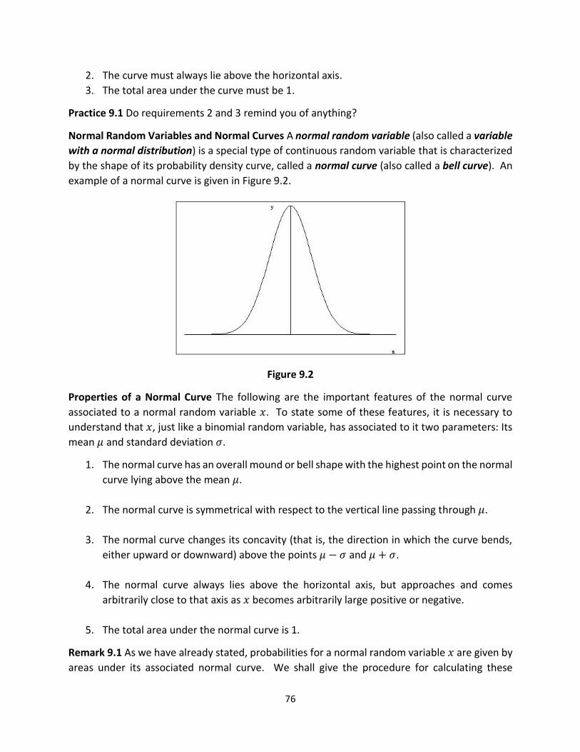
76

2. The curve must always lie above the horizontal axis.

3. The total area under the curve must be 1.

Practice 9.1 Do requirements 2 and 3 remind you of anything?

Normal Random Variables and Normal Curves A normal random variable (also called a variable

with a normal distribution) is a special type of continuous random variable that is characterized

by the shape of its probability density curve, called a normal curve (also called a bell curve). An

example of a normal curve is given in Figure 9.2.

Figure 9.2

Properties of a Normal Curve The following are the important features of the normal curve

associated to a normal random variable 𝑥. To state some of these features, it is necessary to

understand that 𝑥, just like a binomial random variable, has associated to it two parameters: Its

mean 𝜇 and standard deviation 𝜎.

1. The normal curve has an overall mound or bell shape with the highest point on the normal

curve lying above the mean 𝜇.

2. The normal curve is symmetrical with respect to the vertical line passing through 𝜇.

3. The normal curve changes its concavity (that is, the direction in which the curve bends,

either upward or downward) above the points 𝜇 − 𝜎 and 𝜇 + 𝜎.

4. The normal curve always lies above the horizontal axis, but approaches and comes

arbitrarily close to that axis as 𝑥 becomes arbitrarily large positive or negative.

5. The total area under the normal curve is 1.

Remark 9.1 As we have already stated, probabilities for a normal random variable 𝑥 are given by

areas under its associated normal curve. We shall give the procedure for calculating these

77

probabilities shortly (see Theorem 9.1), but we now state a general rule, the Empirical Rule, that

can be used to quickly calculate some probabilities for a normal random variable.

The Empirical Rule If 𝑥 is a normal random variable with mean 𝜇 and standard deviation 𝜎, then

𝑃(𝜇 − 𝜎 ≤ 𝑥 ≤ 𝜇 + 𝜎) ≈ 68%

𝑃(𝜇 − 2𝜎 ≤ 𝑥 ≤ 𝜇 + 2𝜎) ≈ 95%

𝑃(𝜇 − 3𝜎 ≤ 𝑥 ≤ 𝜇 + 3𝜎) ≈ 99.7%

See Exercise 9.4 for a proof of the Empirical Rule.

Example 9.2 The heights, in inches, of adult (over the age of 20) females in the US have an

approximately normal distribution with mean 64 and standard deviation 3. What is the

probability that a randomly chosen adult female in the US is between 58” and 70” tall? What is

the probability that she is at most 58” tall?

Solution Notice that 58” is 2 standard deviations below the mean and 70” is 2 standard deviations

above the mean. Hence, using the Empirical Rule with 2 standard deviations, the probability that

her height lies between these two extremes is about 95%. By the law of the complement, the

probability that her height lies outside these two extremes is 5%. Hence, by the symmetry of a

normal curve, the probability that her height is less than or equal to 58” is 2.5%.

Practice 9.2 What is the probability that a randomly chosen adult female in the US is at least 67”

tall? Hint: Use the Empirical Rule with one standard deviation and the symmetry of a normal

curve.

Remark 9.2 The next theorem provides the method that is commonly used to calculate

probabilities for normal random variables. Its proof requires concepts that we have not

introduced in these notes and, unfortunately, will not be given.

Theorem 9.1 If 𝑥 is a normal random variable with mean 𝜇 and standard deviation 𝜎, and if we

define a new random variable 𝑧 by the formula

𝑧 =𝑥 − 𝜇

𝜎

then 𝑧 is also a normal random variable with mean 0 and standard deviation 1. Moreover, for

any real number 𝑎,

𝑃(𝑥 ≤ 𝑎) = 𝑃(𝑧 ≤𝑎−𝜇

𝜎).

Definitions 9.1 The random variable 𝑧 introduced in Theorem 9.1 is called the standard normal

random variable. The number 𝑎−𝜇

𝜎 is called the 𝒛 score (or standard score) associated to the

number 𝑎, called the 𝒙 score (or raw score). Note: 𝑧 scores should always be rounded to two

decimal places.

78

Remark 9.3 A normal random variable 𝑥 may be measured in a given unit, say inches or pounds,

but the standard normal random variable standardizes the values for 𝑥 by measuring how many

standard deviations they deviate from the mean. Thus 𝑧 is a pure number independent of any

units used for 𝑥. What Theorem 9.1 tells us is that to compute probabilities for any normal

random variable, we standardize and compute the probabilities for the standard normal random

variable 𝑧. The virtue of this procedure is that there are tables that give probabilities for the

standard normal random variable 𝑧. I shall explain in class how to use one of these tables, which

gives probabilities to the left. That is, the table gives

𝑃(𝑧 ≤ 𝑎)

where 𝑎 is any number, rounded to two decimal places, between −3.49 and 3.49.

Computing Probabilities for 𝒛 A table gives probabilities to the left for 𝑧. But what if we want

probabilities to the right? Or in between? These are given by the following formulas:

𝑃(𝑧 ≥ 𝑎) = 1 − 𝑃(𝑧 ≤ 𝑎)

𝑃(𝑎 ≤ 𝑧 ≤ 𝑏) = 𝑃(𝑧 ≤ 𝑏) − 𝑃(𝑧 ≤ 𝑎)

Practice 9.3

a. What does the formula for 𝑃(𝑧 ≥ 𝑎) remind you of?

b. What does the second formula give as the value for 𝑃(𝑧 = 𝑎) = 𝑃(𝑎 ≤ 𝑧 ≤ 𝑎)?

Example 9.3 Let 𝑥 be a random variable that represents the time, in minutes, that it takes a

worker to complete an industrial task. Extensive records show that 𝑥 has an approximately

normal distribution with mean 𝜇 = 15 and standard deviation 𝜎 = 3.14.

a. What is the probability that a randomly selected worker will complete the task in at most

11 minutes?

b. What is the probability that it will take the worker at least 17 minutes to complete the

task?

c. What is the probability that it will take the worker between 18 and 23 minutes to

complete the task?

Solution We have to find the following probabilities:

a. 𝑃(𝑥 ≤ 11)

b. 𝑃(𝑥 ≥ 17)

c. 𝑃(18 ≤ 𝑥 ≤ 23)

The first step is to convert the 𝑥 scores of 11, 17, 18, and 23 into their corresponding 𝑧 scores.

This we do by using the conversion formula given in Theorem 9.1. The results are summarized in

the following table:

79

𝑥 𝑧 =

𝑥 − 15

3.14

11 −1.27 17 0.64 18 0.96

23 2.55

Notice that all the 𝑧 scores have been rounded to 2 decimal places because that is what the table

we are using provides. We now compute the probabilities as follows:

a. 𝑃(𝑥 ≤ 11) = 𝑃(𝑧 ≤ −1.27) = .1020

b. 𝑃(𝑥 ≥ 17) = 𝑃(𝑧 ≥ 0.64) = 1 − 𝑃(𝑧 ≤ 0.64) = 1 − .7389 = .2611

c. 𝑃(18 ≤ 𝑥 ≤ 23) = 𝑃(0.96 ≤ 𝑧 ≤ 2.55) = 𝑃(𝑧 ≤ 2.55) − 𝑃(𝑧 ≤ 0.96)

= .9946 − .8315 = .1631

Exercise 9.1 Let 𝑥 be a normal random variable with mean 𝜇 = 10 and standard deviation 𝜎 =

2.7.

a. Find the probability that 𝑥 is at most 12.

b. Find the probability that 𝑥 is at least 7.

c. Find the probability that 𝑥 is between 5 and 9.

Exercise 9.2 Let 𝑥 be a normal random variable with mean 𝜇 = 12.1 and standard deviation 𝜎 =

1.1.

d. Find the probability that 𝑥 is no more than 10.

e. Find the probability that 𝑥 is not less than 13.

Exercise 9.3 Let 𝑥 be a random variable that represents the weight, in pounds, of a newborn in

the US. Studies show that 𝑥 has an approximately normal distribution with mean 𝜇 = 7.5 and

standard deviation 𝜎 = 1.1.

a. Find the probability that a randomly chosen newborn weighs at most 8 pounds.

b. Find the probability that a randomly chosen newborn weighs at least 5 pounds.

Exercise 9.4 Verify the Empirical Rule that follows Remark 9.1. Hint: For example,

𝑃(𝜇 − 2𝜎 ≤ 𝑥 ≤ 𝜇 + 2𝜎) = 𝑃(−2.00 ≤ 𝑧 ≤ 2.00) = 𝑃(𝑧 ≤ 2.00) − 𝑃(𝑧 ≤ −2.00)

= .9772 − .0228 = .9544 ≈ .95 = 95%

80

Lecture 10: The Central Limit Theorem

We have, at last, reached the heart of the theory that underlies statistical inference. Recall that

the fundamental problem of statistical inference is to draw conclusions about population

parameters based on sample statistics. We shall be primarily concerned with inferences about

the population mean. As we stated at the very beginning of these lectures, we can never be

certain that these inferences are correct, but we can measure the extent of our uncertainty, that

is, we can assign a probability to our conclusions. How is this possible? We need a method that

allows us to calculate the probabilities of observed sample statistics, given certain assumptions

about the distribution of probability in the population. This will allow us to test whether, for

example, an assumed value for a population parameter is consistent with what was observed in

a sample. The aim of this lecture is to develop such a method.

Sampling Distributions The first thing that we need to do is to take a different point of view on

sample statistics. Up to this point, a statistic has been a number calculated from the numbers in

a sample. However, we observed from the very beginning that the value of a statistic cannot be

predicted with certainty before the sample is drawn. Hence, the value of a statistic, before the

sample is drawn, is a random variable.

For definiteness, let us consider the sample mean �̅� based on a random sample of fixed size 𝑛

drawn from a given population. We may think of �̅� as a rule that assigns to each possible

collection of 𝑛 numbers randomly drawn from the population the mean of that collection of

numbers. In this way, we see very clearly that �̅� is indeed a random variable. (Warning: I will

indulge from now on in an abuse of notation in these notes. Sometimes the symbol �̅� indicates

the mean of a particular sample, that is, a number, and sometimes the same symbol indicates a

random variable, that is, a function. No harm will come from this as the context will always clearly

indicate which meaning is intended.) If the sample mean is a random variable, then what is its

probability distribution? What is its expected value? What is its standard deviation? The

distribution of a sample statistic considered as a random variable is called a sampling

distribution. The answers to the above questions about the sampling distribution of the mean

are provided by the following theorem in the case that the population is described by a normal

distribution.

Theorem 10.1 If 𝑥 is a normal random variable with mean 𝜇 and standard deviation 𝜎 and if �̅� is

the sample mean based on a random sample of fixed size 𝑛 drawn from the distribution of 𝑥,

then �̅� is also a normal random variable with mean 𝜇 and standard deviation 𝜎 √𝑛⁄ .

Remark 10.1 Let us try to understand what Theorem 10.1 is telling us. The most important thing

that this theorem tells us is that if we are sampling from a normal population, then the sample

mean will also have a normal distribution. I like to tell my students to remember this in the

following slogan form:

81

Sampling from normal populations gives normal means.

This is a wonderful, and not at all obvious, result because we know how to calculate probabilities

for normal random variables, provided that we know the mean and standard deviation of that

normal random variable. The latter information is also provided by the theorem. It tells us that

the center of the distribution of the sample mean coincides with the center of the population

distribution (not too surprising for you, I hope), but that the variation in the distribution of the

sample mean is less than the variation in the population distribution. The latter assertion

deserves further explanation. (Technical Note: The assertion about the relationship between the

centers and standard deviations of the population distribution and the sampling distribution of

the mean does not require the hypothesis that the population distribution is normal.)

I love the following quote by Sherlock Holmes (taken from Casella and Berger, Statistical

Inference, 2nd ed., p. 1):

“You can, for example, never foretell what any one man will do, but you can say with precision

what an average number will be up to. Individuals vary, but percentages remain constant. So

says the statistician.”

Sherlock Holmes

The Sign of Four

This says beautifully part of what Theorem 10.1 asserts. The variation in individuals is greater

than what one will observe in the averages of groups of individuals. This is intuitively appealing.

Think about it: The height of a randomly chosen human being can vary widely, but the average

heights of, say, 20 randomly chosen human beings will show less variation.

Let us summarize Theorem 10.1 in the form of a table:

Theorem 10.1 Distribution Mean Standard Deviation

Population 𝑥 Normal 𝜇 𝜎

Sample Mean �̅� 𝑛 = sample size

Normal 𝜇 𝜎

√𝑛

Friendly Advice We will be using the information in this table repeatedly. Memorize it!

Example 10.1 Let 𝑥 be a random variable that represents the amount purchased, in dollars, by a

customer of Acme Hardware. Detailed observations show that 𝑥 has an approximately normal

distribution with mean 𝜇 = 28 and standard deviation 𝜎 = 5.7.

82

a. Find the probability that a (that is, one) randomly selected customer spends no more than

$40.

b. Find the probability that a random sample of 10 customers has mean expenditure of at

least $32.

Solution It is extremely important to notice that part a. asks for a probability for 𝑥, but part b.

asks for a probability for �̅�. Don’t forget this. We begin by summarizing the information that we

will need to solve this problem in the form of a table, just like we did above for Theorem 10.1:

Distribution Mean Standard Deviation

𝑥 Normal 28 5.7

�̅� 𝑛 = 10

Normal 28 5.7

√10≈ 1.80

The information in the second row is given to us in the problem. The information in the third

row, except for the sample size of 10, is not. We complete the third row by using the information

in the second row and Theorem 10.1. Notice that I rounded the standard deviation of �̅� to 2

decimal places, as we always do. We already know how to calculate probabilities for normal

random variables. So let’s get to it.

a. We have to find 𝑃(𝑥 ≤ 40). We convert the 𝑥 score of 40 into a 𝑧 score of 2.11 (always

round 𝑧 scores to 2 decimal places), as shown in the following table.

𝑥 𝑧 =

𝑥 − 28

5.7

40 40 − 28

5.7≈ 2.11

Hence

𝑃(𝑥 ≤ 40) = 𝑃(𝑧 ≤ 2.11) = .9826

b. We have to find 𝑃(�̅� ≥ 32). The important thing to remember is that �̅� is a normal

random variable, just like 𝑥, and so we compute probabilities for �̅� just like we do for any

normal random variable. But one must be careful here: When converting �̅� scores to 𝑧

scores, make sure that you use the standard deviation for �̅�, which is 1.80, not 5.7

(remember: �̅� has smaller variation than 𝑥). The conversion is given in the following table:

�̅� 𝑧 =

�̅� − 28

1.80

32 32 − 28

1.80≈ 2.22

Hence

83

𝑃(�̅� ≥ 32) = 𝑃(𝑧 ≥ 2.22) = 1 − 𝑃(𝑧 ≤ 2.22) = 1 − .9868 = .0132

Friendly Advice Please make sure that you thoroughly understand this example. The calculations

that we did in it are absolutely fundamental and must be mastered. It would be fruitless to

proceed otherwise. Check your understanding by doing the following practice problem.

Practice 10.1 Let 𝑥 be a random variable representing the weight, in pounds, of a fish in a lake.

You may assume that 𝑥 has a normal distribution with mean 𝜇 = 3.1 and standard deviation 𝜎 =

0.43.

a. Find the probability that a randomly caught fish weighs at least 6 pounds.

b. Find the probability that a random sample of 40 fish has mean weight not more than 3

pounds.

Remark 10.2 Theorem 10.1 is very useful if we are sampling from a normal population. But what

if the population is known not to be normal? What if we do not know anything about the

distribution in the population? In these cases, Theorem 10.1 is of no help. However, these are

precisely the situations in which the all-important Central Limit Theorem proves useful. The

Central Limit Theorem is one of the most fundamental results in the theory of probability, and

scientific investigators of all sorts use it every day.

Theorem 10.2 (The Central Limit Theorem) If 𝑥 is a random variable with mean 𝜇 and standard

deviation 𝜎, and if �̅� is the sample mean based on a random sample of fixed size 𝑛 drawn from

the distribution of 𝑥, then, provided that 𝑛 is sufficiently large, �̅� will have an approximately

normal distribution with mean 𝜇 and standard deviation 𝜎 √𝑛⁄ .

Remark 10.3 You should read this theorem several times. Superficially, it reads just like Theorem

10.1, but a closer examination reveals significant differences. Let us summarize what the Central

Limit Theorem (CLT from now on) says in the form of a table:

CLT Distribution Mean Standard Deviation

Population 𝑥 Arbitrary 𝜇 𝜎

Sample Mean �̅� 𝑛 ≥ 30

Normal 𝜇 𝜎

√𝑛

Notice that in CLT, no restriction is placed on the distribution of 𝑥 (other than it has to have a

finite mean and variance, conditions that are satisfied in every practical situation). The random

variable 𝑥 may be a binomial random variable or any other type of random variable. This is the

primary reason for the usefulness of CLT.

Notice also the subtle difference in the conclusion of CLT compared to Theorem 10.1: Theorem

10.1 asserts that �̅� is a normal random variable, regardless of the sample size, but CLT states that

�̅� is approximately normal, provided that the sample size 𝑛 is sufficiently large. CLT assumes less

84

about the population than Theorem 10.1 does, but the price is that the sample size has to be

larger and the conclusion is not as sharp. However, in all practical situations, the approximation

given by CLT is good enough. Of course, this raises the obvious question: How big is “sufficiently

large”? My understanding is that 𝑛 ≥ 30 is generally considered large enough to invoke CLT.

Let’s look at an example in which CLT is used to approximate a probability for a binomial random

variable.

Example 10.2 Let’s revisit Example 1.3. I gave there an approximation, namely .01, for the

probability of at least 62 successes, i.e., supporters of Ms. Rodriguez, among 100 randomly

selected registered voters, assuming that Ms. Rodriguez enjoyed only 50% support among all

registered voters. Of course, we may calculate this probability exactly using a binomial random

variable with 𝑛 = 100 and 𝑝 = .5. If you do so (there are freely available online binomial

probability calculators that do this), you will find that the probability of at least 62 successes in

100 trials is .0105, rounded to 4 decimal places.

Let me now explain how I arrived at the approximation .01. The idea is to regard the random

sample of 100 registered voters as being selected from a population modelled by a binomial

random variable with 𝑛 = 1 and 𝑝 = .5. (When 𝑛 = 1, a binomial random variable is also called

a Bernoulli random variable.) From that perspective, the fraction of successes among the 100

registered voters is the mean of the sample (cf. Practice 10.2). Since the sample size is 100, CLT

guarantees that the sample mean has an approximately normal distribution. That is, we may

approximate the binomial probability with 𝑃(�̅� ≥ .62), where �̅� has a normal distribution. See

Figure 10.1 in which the binomial distribution (in blue) and normal approximation (in red) are

shown.

Figure 10.1

85

Since we are assuming that the population distribution has mean 0.5 and, as a consequence,

standard deviation 0.5, we get

𝑃(�̅� ≥ .62) = 𝑃(𝑧 ≥ 2.40) = 1 − 𝑃(𝑧 ≤ 2.40) = 1 − .9918 = .0082

which when rounded to 2 decimal places gives my approximation of .01. Note that the

approximation calculated before rounding to 2 decimal places differs from the actual probability

by only .0023, which is a relative error of about 22%. We may improve considerably on this

approximation by using a “continuity correction.” See Practice 10.3 and 10.4.

Practice 10.2 I have deliberately omitted some details in the computations of Example 10.2 that

I would like you to fill in. Let me help you by asking some questions.

a. Why is the proportion of successes among the 100 registered voters a mean? Hint: Each

time a registered voter is selected, the population random variable takes the value 1 if a

supporter of Ms. Rodriguez is selected and 0 if a non-supporter is selected. So the sample

mean is the average of 100 0’s and 1’s, each of the 1’s representing a success. Isn’t that

exactly the proportion of successes among the 100 registered voters?

b. Why is the population standard deviation 0.5? Hint: The population is modelled by a

binomial random variable with 𝑛 = 1 and 𝑝 = .5. Just use the formula for the standard

deviation of a binomial random variable.

c. Why is 2.40 the 𝑧 score of .62? Hint: Nothing new here. Just remember to use the

standard deviation of the sample mean, not the population standard deviation, when

converting the �̅� score of . 62 = 62 100⁄ into a 𝑧 score.

Practice 10.3 What happens if we try to use the normal approximation to estimate the probability

that the number of successes in 100 trials is exactly 62 when the probability of success is .5?

Answer: We would get an approximation of 0. (Why? Read Example 9.1 again and do Practice

9.3b if you have trouble explaining why.)

To deal with this problem, we use what is called a continuity correction. We shall instead

estimate the probability that the number of successes lies between 61.5 and 62.5. I leave it to

you to do the calculations. That is, calculate 𝑃(𝑟 = 62), where 𝑟 is a binomial random variable

with 𝑛 = 100 and 𝑝 = .5, and then calculate 𝑃(.615 ≤ �̅� ≤ .625), where 𝑥 is a Bernoulli random

variable with 𝑛 = 1 𝑎𝑛𝑑 𝑝 = .5.

Practice 10.4 Redo the approximation in Example 10.2 by using a continuity correction. That is,

rather than using 𝑃(�̅� ≥ .62) for the approximation, use 𝑃(�̅� ≥ .615) instead. Does this improve

the accuracy of the approximation? Moral: When using CLT to approximate probabilities for

discrete random variables that take only integral values, always use a continuity correction.

86

Example 10.3 The scores on a test are modelled by a random variable 𝑥 with mean 𝜇 = 85 and

standard deviation 𝜎 = 12.9. What is the probability that the mean score of a random sample

of 100 test takers is at most 81?

Solution The important point to notice here is that nothing is said about the distribution of 𝑥.

Also, the question asks for the probability of a sample mean result, namely 𝑃(�̅� ≤ 81). CLT

may be applied here because the sample size of 100 is very large. I advise that you summarize

all the information that has been given and that you will need in a table, as follows:

Distribution Mean Standard Deviation

𝑥 Unknown 85 12.9

�̅� 𝑛 = 100

Normal 85 12.9

√100= 1.29

The information in the second row was given in the problem. The third row, which gives us the

information that we need to answer the question, follows from CLT. It is now a simple matter to

convert the �̅� score of 81 into its corresponding 𝑧 score, which is, rounded to 2 decimal places,

−3.10. (Never take such an assertion at face value. Check it by doing the calculation yourself!)

Hence

𝑃(�̅� ≤ 81) = 𝑃(𝑧 ≤ −3.10) = .0010

Remark 10.4 Let’s discuss the result of Example 10.3 in a broader context and from a different

point of view. One way to look at Example 10.3 is that if the population mean is assumed to be

85 (and the population standard deviation is somehow known to be 12.9), then it is extremely

unlikely to get a sample mean of 81 or less in a random sample of size 100. That sample result

lies so far below (more than 3 standard deviations below in fact) the sample mean’s center of 85

that it cannot be explained by chance.

If we did observe a sample mean of at most 81, then there are two possible explanations: Either

a very rare event (one with a probability of only .0010) has occurred or the assumption that the

population mean is 85 has to be rejected. When we discuss hypothesis tests in Lecture 12, we

shall see that the latter explanation is the one that is adopted.

Why? I like to keep the following slogan in mind:

Nature dislikes the unlikely.

This does not mean that unlikely events never occur; of course they do. But if we have to choose

between two alternatives (two “states of nature,” if you will), one in which what is observed is

unlikely and the other in which what is observed is more likely, then the slogan means that we

should choose the latter alternative.

Let’s examine this argument in more detail. The probability of getting a sample mean of 81 or

less, assuming that the population mean is 85, is .0010. That probability is so low that we cannot

87

reasonably explain an observed sample mean of 81 as the result of chance fluctuation in the

sample mean. That implies it is very likely that we will get a similar result if another sample of

size 100 was drawn. Conclusion: The sample observation is very strong evidence against the

assumption that the population mean is 85, and therefore, that assumption has to be rejected in

favor of the hypothesis that the population mean is less than 85. Is it possible that this conclusion

is a mistake? Yes. We can never be sure that we have made the correct decision, but the

probability that we made an error is very low.

Friendly Advice Please read Remark 10.4 several times. The ideas in it are subtle or, at least,

different from what you may be accustomed to, and it takes time, repetition, and thought for

these ideas to be internalized. We shall revisit these ideas when we discuss hypothesis tests in

Lecture 12.

Exercise 10.1 Let 𝑥 be a random variable that represents the time, in minutes, that it takes for

students to complete a final exam. You may assume that 𝑥 has an approximately normal

distribution with mean 𝜇 = 115 and standard deviation 𝜎 = 13.7.

a. What is the probability that a randomly selected student takes at least 140 minutes to

take the final exam?

b. What is the probability that a randomly selected class of 28 students has a mean

completion time of at most 110 minutes?

Exercise 10.2 Let 𝑥 represent the length, in inches, of a machined tube. Then 𝑥 has an

approximately normal distribution with mean 𝜇 = 14 and standard deviation 𝜎 = 0.21. The

manufacturer randomly samples tubes prior to shipment to assure that the average tube length

is not too short, that is, less than the target mean of 14. A random sample of 25 tubes had mean

length 13.87. Is this sample result cause for concern that the tube lengths have a mean less than

14? Hint: Assume that nothing is wrong. That is, that the mean length of the tubes is where it is

supposed to be at 14. What is the probability of getting a sample mean of 13.87 or less under

that assumption?

Exercise 10.3 Jillian walks to work each day. Let 𝑥 be a random variable that represents the

time (in minutes) that it takes Jillian to walk to work. You may assume that 𝑥 has a normal

distribution with mean 𝜇 = 24 and standard deviation 𝜎 = 3.4.

a. Find the probability that on a randomly selected day, Jillian will walk to work in at

most 30 minutes.

c. Find the probability that on 12 randomly chosen days, the mean time for Jillian to

walk to work will be at least 23 minutes.

Exercise 10.4 The weights (in pounds) of adult (18 years or older) males in the US are

approximately normally distributed with mean µ = 187 and standard deviation σ = 21.2.

a. What is the probability that a randomly chosen adult male in the US will weigh no

more than 212 pounds?

88

b. What is the probability that the mean weight of a random sample of 23 adult males

in the US will be at least 177 pounds?

Exercise 10.5 Reliable Taxi has found that the response time (in minutes) for a pickup is

normally distributed with mean µ = 12 and standard deviation 𝜎 = 2.1.

a. What is the probability that the response time for a randomly selected pickup call

will be at most 10 minutes?

b. For a random sample of 19 pickup calls, what is the probability that the sample

mean response time is not less than 12.5 minutes?

Exercise 10.6 Let 𝑥 be a random variable that represents the weight of a lion in a certain region

of Africa. Assume that 𝑥 is normally distributed with mean µ = 259 lbs. and standard deviation

σ = 35.3 lbs.

a. What is the probability that a randomly selected lion from that region will weigh at

least 300 lbs.?

b. Suppose 39 lions are randomly selected and weighed. What is the probability that

the mean weight �̅� of the lions is no more than 247 lbs.?

Exercise 10.7 Roberto jogs 1 mile every day. His record of the times, in minutes, that it takes to

complete the jogs indicates that these are approximately normally distributed with mean µ =

8.2 minutes and standard deviation σ = 1.1 minutes.

a. What is the probability that on a randomly selected day, it will take Roberto at least

10 minutes to complete his jog?

b. If Roberto’s times on 23 randomly selected days are recorded, what is the

probability that the mean time is no more than 8 minutes?

89

Appendix F: Infinity

I have for the most part in these notes avoided dealing with the infinite. This was of course

impossible when discussing continuous random variables, where the assumption of infinitely

precise measurements was tacitly made. The theory becomes much richer and has wider

applicability if we have the language and tools available to discuss infinitely precise

measurements or infinitely repeated activities (such as tossing a coin infinitely many times,

which, although physically impossible, cannot, or, rather, should not, be ruled out conceptually).

We shall in this appendix tackle infinity head on and treat it as a mathematical notion. The

concepts that we introduce will allow us to express some of the ideas that we have previously

encountered more precisely and clearly. The aim of this appendix is to state precisely two

signature theorems in probability theory: The Central Limit Theorem, which we have already

discussed from a non-technical viewpoint, and the Strong Law of Large Numbers, which has not

been discussed at all but is so well known (and misunderstood) that these notes would be

incomplete without it.

Infinities Perhaps the most surprising result in the mathematical theory of the infinite is that

there are different orders or types of infinities. This remarkable insight is due to the German

mathematician Georg Cantor, who we previously encountered as the founder of set theory. As

usual, let us begin with an example.

Example F.1 There are clearly “more” integers than natural numbers. But in a certain sense these

sets have the same number of elements. Both these sets are infinite, and so in what sense can

we say that they each have “the same number of elements?” One way to make sense of such a

statement is to pair each natural number with a unique integer in such a way that every integer

appears once and only once in the pairing. The following table gives one way of doing this:

Natural Numbers

1 2 3 4 5 6 7 …

Integers 0 1 −1 2 −2 3 −3 …

A function is lurking behind the table above. Let 𝑁 denote the set of natural numbers, let 𝑍 (for

“zahlen,” the German word for “numbers”) denote the set of all integers, and let 𝑓: 𝑁 → 𝑍 be

the function defined for each natural number 𝑛 by the following rule:

𝑓(𝑛) =𝑛

2, if 𝑛 is even

𝑓(𝑛) = −𝑛−1

2, if 𝑛 is odd

Practice F.1

a. Find 𝑓(1), 𝑓(2), 𝑓(3), 𝑓(4) and 𝑓(5).

90

b. What are the 41st and 42nd numbers in the list?

The function 𝑓 is said to be a one-to-one correspondence between 𝑁 and 𝑍. This means that

every element in 𝑍 appears as the value under 𝑓 of one, and only one, element in 𝑁. In

terminology to be introduced next, this shows that 𝑍 is countable.

Definitions F.1

1. Finite: A set is finite if it is either empty or there exists a natural number 𝑛 such that the

set may be placed in one-to-one correspondence with the collection of all natural

numbers less than or equal to 𝑛.

2. Infinite: A set is infinite if it is not finite.

3. Countable: An infinite set is countable if it may be placed in one-to-one correspondence

with the set of all natural numbers 𝑁.

4. Uncountable: An infinite set is uncountable if it is not countable.

Remark F.1 The archetypal example of a countable set is the set 𝑁 of all natural numbers itself,

and any set that may be placed into one-to-one correspondence with 𝑁 is also countable, by

definition. Intuitively, an infinite set is countable if you may write all its elements, one after

another, in a list. If you cannot produce such a list, then the set is uncountable.

Example F.2 The set of even natural numbers is countable. Here is a list: 2, 4, 6, 8, …

Practice F.2 Show that the set of odd natural numbers is countable.

Example F.3 The set of all positive rational numbers (that is, fractions) is countable. Here is a list:

1, 1 2,⁄ 2, 1 3⁄ , 3, 1 4⁄ , 2 3⁄ , 3 2⁄ , 4, 1 5⁄ , …

Practice F.3 What are the next three numbers in the above list?

Practice F.4 Show that the set of all fractions (positive, zero, or negative) is countable. Hint: Think

about the way that we listed the integers in Example F.1 and use the list in Example F.3.

Remark F.2 Are all infinite sets countable? No! Our next theorem gives an example of an

uncountable set.

Theorem F.1 The set [0,1] of all real numbers between 0 and 1 is uncountable.

Proof The proof of this theorem presents a bit of a dilemma. In order to show that [0,1] is

uncountable, we have to “prove a negative.” That is, we have to show that it is impossible to list

all the numbers in [0,1]. It is one thing to show that something is possible. Just show how to do

it. But how does one show that something is impossible? Mathematicians have a method, called

a “proof by contradiction,” that is ideally suited for this purpose. The idea is to assume that we

91

have a list of all the real numbers in [0,1], and then to show that the list must omit at least one

number in [0,1]. That’s a contradiction, and it shows that no such list can exist.

Suppose then that there is a list of all the real numbers in [0,1], and, for definiteness, let us

assume that it begins as follows:

0.175268…, 0.051280…, 0.004000…, 0.333333…, 0.777754…, 0.121212…

(We use the decimal representation of real numbers. In order to avoid any ambiguity in that

representation, we only use the representation that ends in a string of 0’s. For example, we use

0.5000…, rather than 0.4999… .) We now construct a number 𝑢 in [0,1] that cannot possibly be

in the above list. Notice that certain digits have been highlighted in bold and underlined in the

numbers above. The idea is that 𝑢 will have its tenths digit different from 1, its hundredths digit

different from 5, its thousandths digit different from 4, its ten-thousandths digit different from

3, and so forth.

We do this by giving a definite rule for choosing the decimal digits of 𝑢 as follows. Let the digit

in the nth decimal place of 𝑢 be 5 if the digit in the nth decimal place of the nth number in the list

is not 5; otherwise, let the digit in the nth decimal place of 𝑢 be 6. That may sound complicated,

but the idea is deceptively simple. We are just making sure that the decimal expansion of the

number 𝑢 is different from the decimal expansion of any number in the list, and by using only

5′s and 6′s, we guarantee that 𝑢 is a number in [0,1] (and also avoid any issue of ambiguity).

Using the numbers displayed in the list above, for example, we obtain the following decimal

expansion for the missing number:

𝑢 = 0.5655 …

(What are the next two digits in the decimal expansion of 𝑢?) It is clear that 𝑢 is in [0,1] and that

it is not in the list. The argument that we have just given is quite general and may be applied to

any alleged list of all the numbers in [0,1] to produce a number in [0,1] that is not in the list. We

conclude that no such list can exist. QED

Remark (Optional) Are there infinities besides those exhibited by 𝑁 and [0,1]? Yes! Cantor

proved the following seemingly innocuous result, but, as we shall see in the remark after its proof,

it has a stunning consequence.

Theorem (Optional) There does not exist a one-to-one correspondence between a nonempty set

and the collection of all subsets of that set.

Proof (Optional) Let 𝑆 be a nonempty set, let 𝒫(𝑆) denote the collection of all subsets of 𝑆 (𝒫(𝑆)

is called the power set of 𝑆), and suppose that there exists a one-to-one correspondence 𝑓: 𝑆 →

𝒫(𝑆). We now show that the existence of 𝑓 leads to a contradiction.

Let 𝐴 = {𝑢 ∈ 𝑆: 𝑢 ∉ 𝑓(𝑢)}. That is, 𝐴 consists of those members of 𝑆 that do not belong to the

subset of 𝑆 with which they are paired by 𝑓. Our hypothesis that 𝑓 is a one-to-one

92

correspondence implies that there exists a unique element 𝑠 ∈ 𝑆 such that 𝑓(𝑠) = 𝐴. Now,

either 𝑠 ∈ 𝐴 or 𝑠 ∉ 𝐴 because there are no other possibilities. On the one hand, 𝑠 ∈ 𝐴 implies,

by the very definition of the set 𝐴, that 𝑠 ∉ 𝑓(𝑠) = 𝐴, a contradiction. On the other hand, 𝑠 ∉ 𝐴

implies, again by the definition of 𝐴, that 𝑠 ∈ 𝑓(𝑠) = 𝐴, another contradiction. QED

Remark (Optional) I am in awe of Cantor’s cleverness. In one stroke of genius he has created an

infinity of infinities! It is a consequence of his theorem that no two of the following infinite sets

are in one-to-one correspondence:

𝑁, 𝒫(𝑁), 𝒫( 𝒫(𝑁)), 𝒫( 𝒫(𝒫(𝑁))), …

Are any of these sets in one-to-one correspondence with [0,1]? Yes. The second one on the list,

𝒫(𝑁), is in one-to-one correspondence with [0,1]. The proof of this fact uses the representation

of a real number in base 2 rather than base 10.

Does this list give all possible infinities? No. The collection of all the elements in the sets in the

list is not in one-to-one correspondence with any set in the list.

Is there an infinity “strictly between” 𝑁 and 𝒫(𝑁)? That’s a deep question, and it does not admit

a simple “yes” or “no” response. Loosely speaking, either response is consistent with the axioms

that are generally accepted as the foundation for set theory.

Limits at Infinity We now ask what happens at infinity in certain infinite lists of numbers (called

infinite sequences). Let’s look at an example.

Example F.4 Do the numbers in the following list “tend” to some definite number?

1, 1 2⁄ , 1 3⁄ , 1 4⁄ , 1 5⁄ , …

The general number in this list is of the form 1 𝑛⁄ for some natural number 𝑛. Intuitively, as 𝑛

becomes arbitrarily large, or as 𝑛 approaches infinity, then 1 𝑛⁄ comes arbitrarily close to 0. We

describe this by saying that “1 𝑛⁄ approaches 0 as n approaches infinity” and write

lim𝑛→∞

1

𝑛= 0

The above equality is read: “The limit of 1 𝑛⁄ as 𝑛 approaches infinity is 0.” Please do not ascribe

any mystical meaning to the appearance of the symbol ∞. The symbol "𝑛 → ∞" is just an

abbreviation for “𝑛 becomes arbitrarily large.”

Practice F.5 Find lim𝑛→∞

(3 −1

𝑛).

Practice F.6 Find lim𝑛→∞

(1 −1

2𝑛 ).

Practice F.7 Does the sequence (−1)𝑛, 𝑛 = 1, 2, 3, … have a limit? No proof is required.

Intuitively, do the numbers in the list eventually come arbitrarily close to exactly one number?

93

Hint: Write the first few numbers of the sequence. An obvious pattern appears, and it will be

clear that the sequence does not come arbitrarily close to one number.

Sums: Finite and Infinite We all know how to add the numbers in a finite list. As we have seen,

this occurs so often in mathematics that we introduced sigma notation to denote such a sum.

For example, if the variable 𝑥 is assumed to vary over all the numbers in a sample, then

∑ 𝑥

denotes the sum of all the numbers in that sample.

We want now to introduce a slight variant of sigma notation that is more useful for our current

purposes. If we have a finite list of 𝑛 numbers (called a finite sequence), say, 𝑥1, 𝑥2, … , 𝑥𝑛, then

we shall abbreviate the sum of these 𝑛 numbers as follows:

𝑥1 + 𝑥2 + ⋯ + 𝑥𝑛 = ∑ 𝑥𝑖

𝑛

𝑖=1

This process of adding a finite sequence of numbers has certain basic properties that should be

clear. We just state these in the next theorem.

Theorem F.2 (Fundamental Properties of Finite Sums)

1. ∑ (𝑥𝑖 + 𝑦𝑖) = ∑ 𝑥𝑖𝑛𝑖=1 + ∑ 𝑦𝑖

𝑛𝑖=1

𝑛𝑖=1

2. If c is any constant, then

∑ 𝑐𝑥𝑖

𝑛

𝑖=1

= 𝑐 ∑ 𝑥𝑖

𝑛

𝑖=1

3. If 𝑥𝑖 ≥ 0 for all 𝑖 = 1, 2, … , 𝑛, then

∑ 𝑥𝑖

𝑛

𝑖=1

≥ 0

Notice that it follows from 2. that

∑ 𝑐

𝑛

𝑖=1

= 𝑐 ∑ 1 = 𝑛𝑐

𝑛

𝑖=1

Applications (Optional) We now give three applications to statistics of the fundamental

properties of finite sums. These applications are not difficult, but they do require a higher level

of proficiency in algebra than I have assumed in the rest of these notes. Hence they are optional

and may safely be skipped without loss if you are not interested.

94

Application F.1 (Optional) The sum of the deviations from the mean in a sample is always 0.

Proof If the numbers in the sample are 𝑥1, 𝑥2, … , 𝑥𝑛, then

∑ (𝑥𝑖 − �̅�)𝑛𝑖=1 = ∑ 𝑥𝑖

𝑛𝑖=1 − ∑ �̅�𝑛

𝑖=1 = 𝑛�̅� − 𝑛�̅� = 0 QED

Practice Show that the sample mean is the unique number with the above property. That is, for

any number 𝑥, ∑ (𝑥𝑖 − 𝑥)𝑛𝑖=1 = 0 if and only if 𝑥 = �̅�.

Application F.2 (Optional) The defining and computational formulas for the sample variance are

equal.

Proof If the numbers in the sample are 𝑥1, 𝑥2, … , 𝑥𝑛, then

∑ (𝑥𝑖 − �̅�)2𝑛𝑖=1

𝑛 − 1=

∑ (𝑥𝑖2 − 2𝑥𝑖�̅� + �̅�2)𝑛

𝑖=1

𝑛 − 1=

∑ 𝑥𝑖2𝑛

𝑖=1 − ∑ 2𝑥𝑖𝑛𝑖=1 �̅� + ∑ �̅�2𝑛

𝑖=1

𝑛 − 1

∑ 𝑥𝑖2𝑛

𝑖=1 − 2�̅� ∑ 𝑥𝑖𝑛𝑖=1 + ∑ �̅�2𝑛

𝑖=1

𝑛 − 1=

∑ 𝑥𝑖2𝑛

𝑖=1 − 2𝑛�̅�2 + 𝑛�̅�2

𝑛 − 1=

∑ 𝑥𝑖2𝑛

𝑖=1 − 𝑛�̅�2

𝑛 − 1

=∑ 𝑥𝑖

2𝑛𝑖=1 −𝑛(

∑ 𝑥𝑖𝑛𝑖=1

𝑛)

2

𝑛−1=

∑ 𝑥𝑖2𝑛

𝑖=1 −1

𝑛(∑ 𝑥𝑖

𝑛𝑖=1 )

2

𝑛−1=

𝑛 ∑ 𝑥𝑖2𝑛

𝑖=1 −(∑ 𝑥𝑖𝑛𝑖=1 )

2

𝑛(𝑛−1) QED

Application F.3 (Optional) The sample mean gives the minimum value for the sum of the squared

deviations of the numbers in a given sample from a fixed number.

Proof If the numbers in the sample are 𝑥1, 𝑥2, … , 𝑥𝑛, then for any number 𝑥,

∑(𝑥𝑖 − 𝑥)2

𝑛

𝑖=1

= ∑(𝑥𝑖2 − 2𝑥𝑖𝑥 + 𝑥2) = ∑ 𝑥𝑖

2

𝑛

𝑖=1

− ∑ 2𝑥𝑖

𝑛

𝑖=1

𝑥 + ∑ 𝑥2

𝑛

𝑖=1

𝑛

𝑖=1

= ∑ 𝑥𝑖2

𝑛

𝑖=1

− 2 (∑ 𝑥𝑖

𝑛

𝑖=1

) 𝑥 + 𝑛𝑥2 = 𝑛 (∑ 𝑥𝑖

2𝑛𝑖=1

𝑛− 2�̅�𝑥 + 𝑥2)

= 𝑛 (∑ 𝑥𝑖

2𝑛𝑖=1

𝑛− �̅�2 + �̅�2 − 2�̅�𝑥 + 𝑥2) = (∑ 𝑥𝑖

2

𝑛

𝑖=1

− 𝑛�̅�2) + 𝑛(𝑥 − �̅�)2

≥ ∑ 𝑥𝑖2

𝑛

𝑖=1

− 𝑛�̅�2 = (𝑛 − 1)𝑠2

because

𝑛(𝑥 − �̅�)2 ≥ 0

Note that we have used in the above computations the following well-known algebraic identity:

(𝑢 − 𝑣)2 = 𝑢2 − 2𝑢𝑣 + 𝑣2

95

It follows that the sum of the squared deviations from 𝑥 of the numbers in the sample is

minimized precisely when 𝑥 = �̅�. In that case, the minimum value is (𝑛 − 1)𝑠2. QED

Practice (Optional) Show that

∑ 𝑥𝑖2

𝑛

𝑖=1

− 𝑛�̅�2 = (𝑛 − 1)𝑠2

(Hint: Examine the computations in the proof of Application F.2 carefully.) Conclude that the

sample variance of a given sample is the smallest value for the “average” of the squared

deviations of the numbers in that sample from a fixed number. More precisely, for a given sample

𝑥1, 𝑥2, … , 𝑥𝑛 and for any number 𝑥,

∑ (𝑥𝑖 − 𝑥)2𝑛𝑖=1

𝑛 − 1≥ 𝑠2

Remark F.3 It often happens in mathematics that we have to consider “infinite sums,” called

infinite series. Let us illustrate this with an example.

Example F.5 A fair coin is tossed until it lands heads. Let 𝑥 be a random variable that counts the

number of tosses required to produce the first heads. Using the multiplication law for

independent events, we obtain the following probability distribution for 𝑥:

𝑘 1 2 3 … 𝑛 …

𝑃(𝑥 = 𝑘) 1

2

1

22

1

22

… 1

2𝑛

…

If this is to be a valid probability distribution, then it is required that

1

2+

1

22+

1

23+ ⋯ +

1

2𝑛+ ⋯ = 1

The left-hand side of the above equality presents a problem: How do we add an infinite sequence

of numbers? We shall abbreviate the sum on the left-hand side of the above equality as

∑1

2𝑖

∞

𝑖=1

Such a sum is an example of an infinite series (in fact, of a very special and important type of

infinite series called a geometric series).

96

We need to be careful about how to interpret infinite sums. The key is that we know how to add

a finite sequence of numbers, and so we define an infinite sum to be the limit of a sequence of

finite sums. That is, we define

∑1

2𝑖

∞

𝑖=1

= lim𝑛→∞

∑1

2𝑖

𝑛

𝑖=1

provided, of course, that this limit exists.

Practice F.8 Show that

lim𝑛→∞

∑1

2𝑖

𝑛

𝑖=1

= 1

Hint: Use the result of Practice F.6 and the following algebraic identity, valid for any number 𝑟 ≠

1 (in particular, for 𝑟 = 1 2⁄ ):

∑ 𝑟𝑖

𝑛

𝑖=1

=𝑟

1 − 𝑟(1 − 𝑟𝑛)

Practice F.9 Does ∑ (−1)𝑖∞𝑖=1 exist? Hint: By definition,

∑(−1)𝑖

∞

𝑖=1

= lim𝑛→∞

∑(−1)𝑖

𝑛

𝑖=1

provided that the limit exists. Show that, in fact, this limit does not exist by calculating some of

the sums on the right-hand side of the above definition and convincing yourself that each such

sum is either −1 (if 𝑛 is odd) or 0 (if 𝑛 is even). So the sums do not approach a definite number

as 𝑛 becomes arbitrarily large.

Remark F.4 It may be shown that infinite sums have the same properties that are given for finite

sums in Theorem F.2. We state this as our next theorem.

Theorem F.3 (Fundamental Properties of Infinite Sums) If ∑ 𝑥𝑖∞𝑖=1 exists, if ∑ 𝑦𝑖

∞𝑖=1 exists, and if

𝑐 is any constant, then ∑ (𝑥𝑖∞𝑖=1 + 𝑦𝑖) exists, ∑ 𝑐𝑥𝑖

∞𝑖=1 exists, and the following statements are

true:

1. ∑ (𝑥𝑖 + 𝑦𝑖) = ∑ 𝑥𝑖∞𝑖=1 + ∑ 𝑦𝑖

∞𝑖=1

∞𝑖=1

2. ∑ 𝑐𝑥𝑖∞𝑖=1 = 𝑐 ∑ 𝑥𝑖

∞𝑖=1

3. If 𝑥𝑖 ≥ 0 for all 𝑖 = 1, 2, …, then

∑ 𝑥𝑖

∞

𝑖=1

≥ 0

97

Integrals In order to give a proper definition of continuous random variables and to state the

Central Limit Theorem precisely, we must consider the continuous analog of infinite sums, called

integrals. I will not give the technical definition of an integral because that belongs properly to

a course in calculus. (If you are interested in learning about calculus, take a look at D. Kleppner

and N. Ramsey, Quick Calculus, 2nd ed., 1985, John Wiley & Sons. Ramsey was awarded a Nobel

Prize in Physics in 1989.) However, there is a very nice and intuitive geometric interpretation of

integrals as net areas that will be more than sufficient for our purposes. Integrals are defined for

a large class of functions, but, again because our purposes are limited, we need only restrict

consideration to integrals of continuous functions, which we now introduce before defining

integrals.

Definition F.2 Continuous Function: If 𝑓: 𝑅 → 𝑅 (remember that 𝑅 denotes the set of all real

numbers) is a function, then we say that 𝑓 is continuous if for any sequence 𝑢1, 𝑢2, … , 𝑢𝑛, … of

real numbers such that lim𝑛→∞

𝑢𝑛 = 𝑢, where 𝑢 is also a real number, we have lim𝑛→∞

𝑓(𝑢𝑛) = 𝑓(𝑢).

Remark F.5: That is, 𝑓 is continuous if it preserves limits of sequences. It is not at all obvious, but

nevertheless true, that a function is continuous if its graph is all of one piece, with no gaps or

jumps.

Example F.6 The functions in Examples E.13-15 are all continuous. Dirichlet’s function in Example

E.12 is pathologically not continuous.

Remark F.7 We may produce new functions from given functions by using the arithmetic

operations of addition and multiplication. These new functions will be continuous if the given

functions are. This is the content of the next definition and the theorem that follows it.

Definition F.3 (New Functions from Old) If 𝑓 and 𝑔 are functions from 𝑅 to 𝑅 and if 𝑐 is any

constant, then we may define new functions 𝑓 + 𝑔, called the sum, and 𝑐𝑓, called a constant

multiple, for all real numbers 𝑢 as follows:

a. (𝑓 + 𝑔)(𝑢) = 𝑓(𝑢) + 𝑔(𝑢)

b. (𝑐𝑓)(𝑢) = 𝑐𝑓(𝑢)

Theorem F.4 Sums and constant multiples of continuous functions are continuous.

Example F.7 Since 𝑓(𝑢) = 𝑢2 and 𝑔(𝑢) = 3𝑢 + 2 are continuous (look at their graphs in Figures

E.1 and E.2), then so are

(𝑓 + 𝑔)(𝑢) = 𝑓(𝑢) + 𝑔(𝑢) = 𝑢2 + 3𝑢 + 2

(8𝑓)(𝑢) = 8𝑓(𝑢) = 8𝑢2

The graphs of 𝑓 + 𝑔 𝑎𝑛𝑑 8𝑓 are shown in Figures F.1 and F.2, respectively.

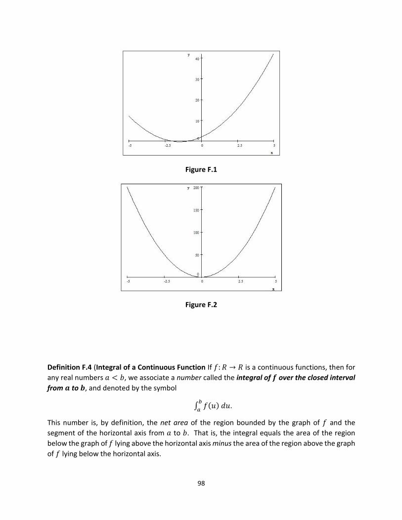
98

Figure F.1

Figure F.2

Definition F.4 (Integral of a Continuous Function If 𝑓: 𝑅 → 𝑅 is a continuous functions, then for

any real numbers 𝑎 < 𝑏, we associate a number called the integral of 𝒇 over the closed interval

from 𝒂 to 𝒃, and denoted by the symbol

∫ 𝑓(𝑢) 𝑑𝑢𝑏

𝑎.

This number is, by definition, the net area of the region bounded by the graph of 𝑓 and the

segment of the horizontal axis from 𝑎 to 𝑏. That is, the integral equals the area of the region

below the graph of 𝑓 lying above the horizontal axis minus the area of the region above the graph

of 𝑓 lying below the horizontal axis.

99

Note: The symbol ∫, which looks like an elongated “S” and is meant to suggest “sum,” is called

an “integral sign” and was introduced by one of the founders of calculus, the German

mathematician Leibniz. Leibniz thought of the integral as a sum of infinitely many areas of tiny

rectangles of height 𝑓(𝑢) and width 𝑑𝑢, and thus the integral gives the area under the graph of

𝑓. The conception of the integral as area is very useful, but it should be noted that integrals arise

in very many contexts, for example, in physics where it has a myriad of interpretations. However,

thinking of the integral as area is fine for our needs.

Example F.7 If we examine the graph of the function 𝑓(𝑢) = 2 over the closed interval [0,3] =

{𝑢 ∈ 𝑅: 0 ≤ 𝑢 ≤ 3} (see Figure F.3) and recall that the area of a rectangle is, by definition, the

product of its base and its height, then

∫ 2 𝑑𝑢 = 63

0

Figure F.3

Example F.8 If we examine the graph of the function 𝑓(𝑢) = 𝑢 over the closed interval [−2,1] =

{𝑢 ∈ 𝑅: − 2 ≤ 𝑢 ≤ 1} (see Figure F.4) and recall that the area of a triangle is one-half the

product of its base and height, then

∫ 𝑢 𝑑𝑢 = −3

2

1

−2

100

Figure F.4

Remark F.8 If 𝑓(𝑢) ≥ 0 for all real numbers 𝑢, then ∫ 𝑓(𝑢) 𝑑𝑢𝑏

𝑎 just gives the area of the region

under the graph of 𝑓 lying over the closed interval from 𝑎 to 𝑏. The integral has the same

fundamental properties as finite and infinite sums. We state this fact in the following theorem.

Theorem F.5 (Fundamental Properties of Integrals) If 𝑓 and 𝑔 are continuous functions 𝑅 → 𝑅

and if 𝑐 is any constant, then

1. ∫ [𝑓(𝑢) + 𝑔(𝑢)]𝑏

𝑎𝑑𝑢 = ∫ 𝑓(𝑢) 𝑑𝑢

𝑏

𝑎+ ∫ 𝑔(𝑢) 𝑑𝑢

𝑏

𝑎

2. ∫ 𝑐𝑓(𝑢) 𝑑𝑢 = 𝑐𝑏

𝑎∫ 𝑓(𝑢) 𝑑𝑢

𝑏

𝑎

3. If 𝑓(𝑢) ≥ 0 for all real numbers 𝑢, then

∫ 𝑓(𝑢) 𝑑𝑢 ≥ 0𝑏

𝑎

Definition F.5 Let 𝑓: 𝑅 → 𝑅 be a function. Then we call 𝑓 a probability density function (and call

its graph a probability density curve) if it satisfies the following three requirements:

a. 𝑓 is continuous

b. 𝑓(𝑢) ≥ 0 for all real numbers 𝑢

c. ∫ 𝑓(𝑢) 𝑑𝑢∞

−∞= 1

Notes:

1. Requirement a. is more restrictive than necessary. There exist many examples of

probability density functions that are not continuous. We impose requirement a. just for

simplicity.

101

2. All that requirement c. means is that the total area under the graph of 𝑓 is 1.

Example F.9 The function 𝑓(𝑢) =1

𝜋(1+𝑢2) is a probability density function. See Figure F.5.

Figure F.5

Discrete vs. Continuous Random Variables We now have enough concepts to give proper

definitions of discrete and continuous random variables.

Definitions F.6 Let 𝑆 be the sample space associated to a random experiment and let 𝑥: 𝑆 → 𝑅

be a random variable.

1. Discrete Random Variable: We say that 𝑥 is discrete if there exists a finite or countable

set of real numbers 𝑘1, 𝑘2, 𝑘3, … such that

∑ 𝑃(𝑥 = 𝑘𝑖) = 1

𝑖

Comment: Intuitively, this says that a random variable is discrete if, with probability 1, it

takes its values in a finite or countable set. All random variables defined on finite sample

spaces, such as binomial random variables, are discrete, and the random variable in

Example F.5 is also discrete.

2. Continuous Random Variable: We say that 𝑥 is continuous if there exists a probability

density function 𝑓: 𝑅 → 𝑅 such that for any real number 𝑎,

𝑃(𝑥 ≤ 𝑎) = ∫ 𝑓(𝑢) 𝑑𝑢𝑎

−∞

Comment: The integral in the preceding equation is just the area of the region under the

graph of 𝑓 lying over the interval of numbers to the left of the number 𝑎. Thus a random

variable is continuous if its probabilities are given by areas under a probability density

102

curve. (Note: In the probability literature, what we have called a continuous random

variable is referred to as an absolutely continuous random variable.)

3. Normal Random Variable: We say that 𝑥 is normal if it is continuous and has a probability

density function of the form (see Figure F.6)

𝑓(𝑢) =1

√2𝜋𝜎𝑒−

12

(𝑢−𝜇

𝜎)

2

Figure F.6

Comment: We may define the expected value (also called mean) and standard deviation

of a continuous random variable in analogy with Definitions 7.1.3-5 by replacing sums

everywhere with integrals. If we do so, then the constants 𝜇 and 𝜎 that appear above

turn out to be the mean and standard deviation, respectively, of the normal random

variable 𝑥. If 𝜇 = 0 and 𝜎 = 1, then we obtain the standard normal random variable 𝑧.

The number 𝑒 = 2.71828 … is a transcendental number that appears in models of

physical processes that exhibit exponential growth or decay. Its formal definition is as

follows:

𝑒 = ∑1

𝑘!

∞

𝑘=0

Practice F.10 Calculate the sum of the first seven terms in the definition of 𝑒. That is,

compute 1

0!+

1

1!+

1

2!+

1

3!+

1

4!+

1

5!+

1

6!

The transcendental number 𝜋 = 3.14159 … gives the area of a circle of radius 1. It is

fascinating that both 𝑒 and 𝜋, fundamental constants of nature, should appear in the

probability density function of the normal random variable.

103

Two Limit Theorems in Probability The two theorems that we are about to state are high points

of the classical theory of probability. The first, the Strong Law of Large of Numbers (SLLN), gives

some theoretical support for the so-called frequentist interpretation of probability, and the

second is the precise statement of the Central Limit Theorem (CLT).

Both theorems involve the notion of an “independent and identically distributed” sequence 𝑥1,

𝑥2, 𝑥3, … of random variables (repeat: each 𝑥𝑖 is a random variable, that is, a function, not a

number). Roughly, an infinite sequence of random variables is “independent’’ if the probability

that any one random variable in the sequence takes values in a particular set is unaffected by the

sets of values taken by any other finite collection of random variables in the sequence. The

sequence is “identically distributed” if all the random variables have the same probability

distribution. Intuitively, a sequence of random variables is “independent and identically

distributed” if, for any particular 𝑛, the collection of the first 𝑛 random variables in the sequence

forms a random sample from a population with a given probability distribution.

Theorem F.6 (The Strong Law of Large Numbers) If 𝑥1, 𝑥2, 𝑥3, … is a sequence of independent

and identically distributed random variables, each with the common finite mean 𝜇, then

𝑃 ( lim𝑛→∞

∑ 𝑥𝑖𝑛𝑖=1

𝑛= 𝜇) = 1

Remark F.6 SLLN says that with probability 1, the sample mean will approach the population

mean as the sample size becomes arbitrarily large. That is intuitively clear, I hope. But SLLN says

more. Suppose that 𝐴 is an event associated to a random experiment. Assigned to 𝐴 is its

probability 𝑃(𝐴), and , as far as the mathematical theory of probability is concerned, how this

assignment is made is irrelevant, as long as the end result satisfies certain requirements.

However, we have from the very beginning used long-term relative frequency to motivate the

concept of probability. It is very satisfying that we may now reconcile the abstractly given

probability 𝑃(𝐴) with the long-term relative frequency of 𝐴.

The idea is that we may take each 𝑥𝑖 in the statement of SLLN to be the Bernoulli random variable

defined by 𝑥𝑖 = 1, if 𝐴 occurs, and 𝑥𝑖 = 0, if 𝐴𝑐 occurs. Notice that using Definition 7.1.3, we

find that the mean of each 𝑥𝑖 is

𝜇 = 0 ∙ 𝑃(𝑥𝑖 = 0) + 1 ∙ 𝑃(𝑥𝑖 = 1) = 0 ∙ 𝑃(𝐴𝑐) + 1 ∙ 𝑃(𝐴) = 𝑃(𝐴).

Notice also that the ratio

∑ 𝑥𝑖𝑛𝑖=1

𝑛

is just the relative frequency of the event 𝐴 in 𝑛 trials of the random experiment. We see then

that SLLN asserts that with probability 1, in any randomly chosen infinite sequence of trials, the

limit of the relative frequency of the event A as the number of trials becomes arbitrarily large will

104

equal 𝑃(𝐴). It is important to understand that this is not a definition of probability, but rather a

theorem, that is, a consequence, of the mathematical theory of probability.

Theorem F.7 (The Central Limit Theorem) If 𝑥1, 𝑥2, 𝑥3, … is a sequence of independent and

identically distributed random variables, each with the common finite mean 𝜇 and finite standard

deviation 𝜎, then for any real number 𝑎,

lim𝑛→∞

𝑃(

∑ 𝑥𝑖𝑛𝑖=1

𝑛−𝜇

𝜎 √𝑛⁄≤ 𝑎) = ∫

1

√2𝜋𝑒−

1

2𝑢2

𝑑𝑢𝑎

−∞

Remark F.7 CLT is a lovely result. It says that in the limit, the sample mean always has a normal

distribution, independently of the population distribution. This is both unexpected and deep,

two hallmarks of a great theorem. The normal distribution, born of the practical need to

approximate certain sums that were formidable to calculate directly, lies at the heart of the

mathematical theory of probability. See Figures F.7 and F.8 for comparisons of a binomial

distribution (in blue) with an approximating normal distribution (in red). Note how the

approximation improves with the sample size.

Figure F.7

105

Figure F.8

106

Lecture 11: Confidence Intervals

Introduction We have developed enough of the theory of probability to allow us to consider a

fundamental problem in statistics: How do we estimate an unknown population parameter based

only on information contained in a random sample? To be specific, we shall consider the problem

of estimating the population mean 𝜇. The procedure we shall develop is based on random

samples that may be small, say less than 30, and for that reason, it is necessary to assume that

the population has a normal distribution. Also, we shall assume that the population standard

deviation 𝜎 is unknown. This describes a situation that an investigator may encounter in practice.

We may thus state the problem at hand as follows:

Problem Estimate the population mean 𝜇 based on a random sample of size 𝑛 drawn from a

population modelled by a random variable 𝑥 with a normal distribution and unknown standard

deviation 𝜎.

The estimate will consist of an interval of numbers that with high confidence (and thus called a

“confidence interval”) contains the true population mean 𝜇. Let us look at a typical confidence

interval problem.

Example 11.1 What is the mean price of a gallon of milk in New York City? An investigator

interested in this question drew a random sample of 6 grocery stores in New York City and found

that the sample mean price (in dollars) of a gallon of milk was �̅� = 3.50. The sample standard

deviation was 𝑠 = 0.72. You may assume that the price of a gallon of milk in New York City has

an approximately normal distribution. Find a 95% confidence interval for the true population

mean price (in dollars) 𝜇 of a gallon of milk in New York City.

We want to calculate an interval of numbers that with 95% confidence, contains the true

population mean price (in dollars) 𝜇 of a gallon of milk in New York City. What information do

we have to calculate this interval? All we have is the sample mean and standard deviation of a

random sample of size 6. Notice that the sample size is small. Notice also the assumption that

prices of a gallon of milk in New York City are approximately normal. It turns out that this

hypothesis will allow us to build a confidence interval entirely on the basis of the sample mean

and standard deviation. Before we do this, we need to develop some theory. The solution to the

above example may be found at the end of this lecture.

Friendly Advice Before proceeding, let me give you a bit of friendly advice. I am about to spell

out some of the theoretical foundation underlying confidence intervals, and then I shall give a

procedure for actually calculating confidence intervals. I do not expect you to completely

understand the theoretical portion. This is an introductory course, and all that I shall ask of you

is that you be able to calculate confidence intervals. However, it is important that you

understand the meaning of a confidence interval, and I shall explain that near the end of this

lecture.

107

Theory of Confidence Intervals We know that when drawing random samples of size 𝑛 from a

population described by a normally distributed random variable 𝑥 with mean 𝜇 and standard

deviation 𝜎, the sample mean �̅� will have a normal distribution with mean 𝜇 and standard

deviation 𝜎 √𝑛⁄ . Prior to drawing the random sample from the distribution of 𝑥, we may

determine the probability that the sample mean �̅� lies within a fixed multiple, which we will for

the moment denote by the letter 𝑘, of 𝜎 √𝑛⁄ from 𝜇. That is to say, we may calculate the

following probability:

𝑃 (𝜇 − 𝑘𝜎

√𝑛≤ �̅� ≤ 𝜇 + 𝑘

𝜎

√𝑛) = 𝑐 (1)

where we shall require the probability 𝑐, called the “confidence level,” to be high, customarily,

. 9 or . 95 or . 99 .

Remarks 11.1

1. We actually begin by specifying 𝑐, and then we find the multiple 𝑘. This is facilitated by tables

designed for that purpose. I shall give the details in class.

2. The probability in (1) is in fact just

𝑃(−𝑘 ≤ 𝑧 ≤ 𝑘) = 𝑐 (2)

where 𝑧 is the standard normal random variable defined by

𝑧 =�̅� − 𝜇

𝜎 √𝑛⁄

3. The probability in (1) may also be rewritten in the equivalent form

𝑃 (�̅� − 𝑘𝜎

√𝑛≤ 𝜇 ≤ �̅� + 𝑘

𝜎

√𝑛) = 𝑐 (3)

Note: I have omitted some intermediate calculations in Remarks 2 and 3 above, so it may not be

clear to you that what I have asserted is true. Please don’t let that deter you from proceeding.

The equation (3) is the important one; just accept it and move on.

In the form (3), we see that prior to drawing the random sample, the probability that the

unknown population mean 𝜇 will lie in the interval [�̅� − 𝑘𝜎

√𝑛, �̅� + 𝑘

𝜎

√𝑛] is 𝑐. The endpoints of

the latter interval are random variables because they depend on the random variable �̅�, and so

it makes sense to speak of the probability that 𝜇 , a definite but unknown number, lies in that

interval.

If you think carefully for a moment, then you will realize that there is a problem with the interval

determined above by the confidence level 𝑐: It requires knowledge of the population standard

deviation 𝜎, which we do not know. All we know is the information provided by the random

sample. The natural solution is to substitute the sample standard deviation 𝑠 for 𝜎; the intuition

108

being that provided the sample is random, 𝑠 should give a reasonable approximation to 𝜎. This

is what we shall do, but it introduces a technicality.

We know that the random variable

𝑧 =�̅� − 𝜇

𝜎 √𝑛⁄

is the standard normal random variable. However, if we substitute 𝑠 for 𝜎, we obtain a new

random variable, traditionally denoted by 𝑡 (called “Student’s 𝑡”):

𝑡 =�̅� − 𝜇

𝑠 √𝑛⁄

This is where the full force of our assumption that the population is normally distributed comes

into play. Based on that assumption, the probability distribution of 𝑡 has been derived, and it is

then possible to determine the number 𝑡𝑐 (called the “critical value” corresponding to the

confidence level 𝑐) such that

𝑃 (�̅� − 𝑡𝑐

𝑠

√𝑛≤ 𝜇 ≤ �̅� + 𝑡𝑐

𝑠

√𝑛) = 𝑐.

(Notice that I have replaced 𝑘 with the more commonly used symbol 𝑡𝑐.) The quantity 𝑡𝑐𝑠

√𝑛 that

appears in the above probability is called the “maximal margin of error” and is denoted by 𝐸:

𝐸 = 𝑡𝑐𝑠

√𝑛.

We thus see that prior to drawing the random sample from the population distribution, there is

a probability c that the true population mean 𝜇 will lie in the random interval

[�̅� − 𝐸, �̅� + 𝐸].

This interval is “random” because its left and right endpoints depend on the random variables �̅�

and 𝑠 .

The critical value 𝑡𝑐 , as the notation suggests, depends on 𝑐. However, it also depends on the

number 𝑛 − 1, called the “degrees of freedom” and denoted by 𝑑. 𝑓.:

𝑑. 𝑓. = 𝑛 − 1

Let me explain why 𝑡𝑐 depends on the degrees of freedom and thus on the sample size. Unlike

the case of the standard normal random variable 𝑧, whose distribution is independent of the

sample size, the distribution of 𝑡 varies with the sample size. The random variable 𝑡 shares some

similarities with the standard normal random variable 𝑧, such as a symmetric bell-shaped

probability density curve and mean 0, but its standard deviation depends on the sample size n.

That is the reason why the critical value depends on the sample size. Finding the critical value

109

once we have specified the confidence level and sample size is easy. All we have to do is look up

the critical value in a table. I shall explain how to do this in class.

Procedure for Calculating Confidence Intervals Having presented the above theoretical

foundation, I shall now outline a procedure for actually calculating a confidence interval for the

population mean 𝜇 with specified confidence level 𝑐:

Step 1: Set the confidence level 𝑐, draw a random sample of size n from the population, and

calculate the sample mean �̅� and the sample standard deviation 𝑠. Note that in a problem, this

information will be provided to you.

Step 2: Calculate the degrees of freedom 𝑑. 𝑓. = 𝑛 − 1.

Step 3: Use a table to find the critical value 𝑡𝑐 corresponding to the confidence level 𝑐 and degrees

of freedom 𝑑. 𝑓.

Step 4: Calculate the maximal margin of error 𝐸 = 𝑡𝑐𝑠

√𝑛. For convenience, we shall always round

off the maximal margin of error to two decimal places.

Step 5: Calculate �̅� − 𝐸 and �̅� + 𝐸.

Step 6: Conclude that a 100𝑐% confidence interval for the true population mean 𝜇 is

[�̅� − 𝐸, �̅� + 𝐸].

The Meaning of a Confidence Interval The statement in Step 6 means that prior to drawing the

random sample and calculating the confidence interval, there is a high probability 𝑐 that the

confidence interval will contain the true population mean 𝜇. This is an important point that is

worth repeating and elaborating for emphasis. We will never know the true value of the

population mean 𝜇. However, before we draw a random sample from the population, we know

that a random interval, which we will calculate once we have the sample data, will contain the

unknown parameter 𝜇 with a high probability 𝑐 that we set.

We cannot be certain that any particular confidence interval that we calculate will in fact contain

the true population mean 𝜇, but if we calculate many, many confidence intervals using the above

procedure (perhaps it would be better to imagine thousands of investigators, each using the

procedure above to calculate a confidence interval for the particular population mean that is of

interest to them), then we can say that approximately 100𝑐% of these will in fact contain 𝜇. It is

this probabilistic interpretation that underlies the use of the word “confidence.”

Solution to Example 11.1

Step 1: 𝑐 = 95% = .95, 𝑛 = 6, �̅� = 3.50, 𝑠 = 0.72

Comment: All this information is given in the statement of the problem. Notice that the

confidence level is converted from a percent to a decimal.

Step 2: 𝑑. 𝑓. = 𝑛 − 1 = 6 − 1 = 5

110

Step 3: Using a table, we find that 𝑡𝑐 = 2.571.

Comment: As noted earlier, I shall explain in class how to find 𝑡𝑐 from a table.

Step 4: 𝐸 = 𝑡𝑐𝑠

√𝑛= 2.571 ∙

0.72

√6= 0.755 … ≈ 0.76

Comment: Notice that we round 𝐸 to two decimal places. Notice also that we use the sample

size 𝑛, not 𝑛 − 1, in the formula for 𝐸.

Step 5: �̅� − 𝐸 = 3.50 − 0.76 = 2.74, �̅� + 𝐸 = 3.50 + 0.76 = 4.26

Step 6: The 95% confidence interval for the true population mean price (in dollars) 𝜇 of a gallon

of milk in New York City is [2.74, 4.26].

Comment: We are 95% confident that the average price of a gallon of milk in New York City lies

between $2.74 and $4.26. That is to say, if this procedure were repeated, for example, 1000

times, then about 950 of the confidence intervals will in fact contain the true population mean

price.

Exercise 11.1 A random sample of the price (in dollars) of a tablet at 6 online stores had a mean

of 𝑥 = 125 and a standard deviation of s = 13.25. Find a 90% confidence interval for the

population mean price of the tablet at all online stores. You may assume that the prices of the

tablet at all online stores has an approximately normal distribution.

Exercise 11.2 The price (in dollars) of a statistics textbook bought online can vary depending on

the online store. A random sample of 24 online stores had mean price 𝑥 = 209.75 and

standard deviation 𝑠 = 23.14. You may assume that the online prices have an approximately

normal distribution. Find a 90% confidence interval for the population mean µ of the online

price of the statistics textbook. Give your answer rounded to 2 decimal places.

Exercise 11.3 A random sample of 13 tablets had a mean battery life of �̅� = 8 hours and a

standard deviation of 𝑠 = 2.5 hours. Assume that the battery life of tablets has a normal

distribution. Find a 99% confidence interval for the population mean battery life of all tablets.

Exercise 11.4 A random sample of 40 families has mean annual income �̅� = 45 (in thousands of

dollars) with standard deviation 𝑠 = 9.3. You may assume that family annual incomes have an

approximately normal distribution. Find a 95% confidence interval for the population mean

family annual income 𝜇.

Exercise 11.5 A random sample of 20 stores has mean annual sales �̅� = 203 (in thousands of

dollars) and standard deviation 𝑠 = 25.3. You may assume that annual sales of all stores are

approximately normally distributed. Find a 90% confidence interval for the population mean

annual sales 𝜇 of all stores.

111

Exercise 11.6 A random sample of prices in thousands of dollars for 12 homes had mean �̅� =

$105.8 and standard deviation 𝑠 = $20.5. Assume that home prices are normally distributed.

Find a 95% confidence interval for the population mean home price.

Exercise 11.7 A random sample of prices of sleeping bags contained 20 prices. The sample

mean was �̅� = $83.75, and the sample standard deviation was 𝑠 = $28.97. Assume that the

prices of sleeping bags are normally distributed. Find a 90% confidence interval for the

population mean price of all sleeping bags.

112

Lecture 12: Hypothesis Tests

We have seen how to estimate an unknown population mean by a confidence interval. We now

want to adopt a different point of view: How do we decide if the population mean has changed

from some normal or historical or claimed value? Perhaps it is best to begin with a typical

hypothesis test problem to set the stage.

Example 12.1 The average resting heart rate, in beats per minute, for a healthy adult male is 80.

John is an adult male, and his doctor is concerned that John’s heart rate is elevated. A random

sample of 10 of John’s resting heart rates has mean rate �̅� = 97. Let 𝑥 be a random variable that

represents John’s resting heart rate. You may assume that 𝑥 has an approximately normal

distribution with standard deviation 𝜎 = 20. Does the above sample result provide strong

evidence that John’s heart rate is elevated? Use a 5% level of significance.

What is at issue here is whether John’s average heart rate is above the normal value of 80. The

sample result suggests that it is, but averages vary unpredictably from sample to sample. Isn’t it

possible that John’s average heart rate is in fact 80, but by virtue of pure chance or random

fluctuation, the sample mean turns out to be higher than 80? We must admit that this is possible.

However, how likely is it that this happens? Is the sample average of 97 so far above the normal

value of 80 that it is unlikely to be the result of chance variation? That is what we have to decide.

Theory of Hypothesis Tests Having set the stage with an example, let us develop the theoretical

framework for a hypothesis test problem. First, we shall consider hypothesis tests of the

population mean 𝜇, and second, we shall assume for simplicity that the population has a normal

distribution with known standard deviation 𝜎. This is unlikely to occur in practice, but it allows

us to focus on the essential ideas.

Null versus Alternative Hypotheses There will be two competing hypotheses about the

population mean 𝜇. One is called the “null” hypothesis, denoted 𝐻0, and the other is called the

“alternative” hypothesis, denoted 𝐻1. The structure of these hypotheses is as follows:

𝐻0: 𝜇 = 𝑘

Comment: 𝑘 is some normal or historical or claimed value of the population mean 𝜇

𝐻1: 𝜇 < 𝑘 (if the sample mean < 𝑘) or

𝜇 > 𝑘 (if the sample mean > 𝑘)

Remarks 12.1

1. Notice that the null hypothesis is always the assertion that the population mean 𝜇 equals

some conventional value. That conventional value may be based on the norm or historical

experience or some claim. Think of it as the assertion that nothing is going on (hence the

designation “null”) and that the sample result is within the range of chance variation.

113

2. Notice that the alternative hypothesis can be one of two types, depending on the result

obtained in the sample. If the sample mean is less (respectively, more) than the

conventional value in the null hypothesis, then the alternative hypothesis is that the

population mean is less (respectively, more) than that conventional value. Null

hypotheses are based on norms or historical experiences or claims, whereas alternative

hypotheses are based on sample results. Actually, there is a third variant of the

alternative hypothesis in which the population mean is asserted to be different from the

conventional value. We will not consider that variant here, again for the sake of keeping

things simple.

Level of Significance We are going to make a decision. Either we shall reject 𝐻0, in which case

we conclude that the sample result deviates so far from the conventional value that it cannot be

explained by chance, or we shall fail to reject 𝐻0, in which case we conclude that there simply is

not enough evidence in the sample to overturn the assumption that nothing is going on (that is

to say, the observed sample result may be reasonably accounted for by chance). This decision

introduces the possibility of error, which is described in the table below.

𝐻0 is true 𝐻0 is false

Reject 𝐻0 Type I error Correct decision

Do not reject 𝐻0 Correct decision Type II error

We thus see that there are two possible types of error: Rejecting the null hypothesis when it is in

fact true (Type I error) or failing to reject the null hypothesis when it is in fact false (Type II error).

The custom is that a Type I error is, in general, the more serious one, and the procedure gives

precedence to minimizing the probability of making a Type I error. The probability of a Type I

error is called the “level of significance” of the hypothesis test and is denoted by the Greek letter

𝛼 (read: “alpha”). Customarily, 𝛼 is set low by the investigator, either at 1% = .01 or 5% = .05.

P-value and the Decision The default hypothesis is the null hypothesis. The P-value quantifies

the chance of getting the sample result or something more extreme (as determined by the

alternative hypothesis) under the assumption that the null hypothesis is true. Hence we have

the following definition:

Definition 12.1

If 𝐻1: 𝜇 < 𝑘, then P-value = 𝑃(�̅� ≤ value obtained in sample, when 𝜇 = 𝑘)

If 𝐻1: 𝜇 > 𝑘, then P-value = 𝑃(�̅� ≥ value obtained in sample, when 𝜇 = 𝑘)

Notice that the inequality in the P-value is determined by the inequality in the alternative

hypothesis. Notice also that when computing the P-value, the population mean is assumed to

114

equal the conventional value in the null hypothesis. Think of the P-value as the attempt to explain

the sample result as chance variation under the assumption that the null hypothesis is true.

The idea is as follows. If the P-value is small, then it is unlikely that the sample result is due to

chance variation, and this is evidence against the null hypothesis. If the P-value is not small, then

the sample result may be accounted for by chance, and this means that there is insufficient

evidence to reject the null hypothesis. Of course, this raises the obvious question: What is

“small”? The answer is that “small” is determined by the level of significance. The decision-

making procedure is the following:

If P-value ≤ 𝛼, then reject 𝐻0.

If P-value > 𝛼, then do not reject 𝐻0.

This completes our discussion of some of the theory underlying a hypothesis test. Let us now

outline a procedure for answering a hypothesis test problem.

Procedure for a Hypothesis Test

Step 1: State the null (𝐻0) and alternative (𝐻1) hypotheses.

Step 2: Specify the level of significance 𝛼 as a decimal.

Step 3: Calculate the P-value.

Step 4: Make a decision: Either reject 𝐻0, if P-value ≤ 𝛼, or do not reject 𝐻0, if P-value > 𝛼.

We shall illustrate this procedure by returning to the example given above.

Solution to Example 12.1

Step 1: 𝐻0: 𝜇 = 80, 𝐻1: 𝜇 > 80

Comment: A healthy adult male is supposed to have an average resting heart rate of 80, but

John’s sample average resting heart rate of 97 is above 80. Be careful here: Never use the sample

result (in this case, the sample mean of 97) in the statement of the null or alternative hypothesis.

Step 2: 𝛼 = 5% = .05

Comment: The level of significance is given in the problem.

Step 3: P-value = 𝑃(�̅� ≥ 97, when 𝜇 = 80) = 𝑃(𝑧 ≥ 2.69) = 1 − 𝑃(𝑧 ≤ 2.69) = 1 − .9964 =

.0036

Comment: This is the probability of getting a sample mean resting heart rate of at least 97 when

John’s true mean heart rate is 80. Notice that we converted the �̅�-score of 97 to a 𝑧-score of

2.69, our usual procedure for computing probabilities for normal random variables.

Step 4: Reject 𝐻0 at the 5% level of significance because P-value = .0036 ≤ .05 = 𝛼

115

Comment: It is extremely unlikely, if John’s true average resting heart rate is 80, to get a sample

mean resting heart rate of at least 97. Hence that sample result cannot be explained by chance

under the assumption that the null hypothesis is true. The sample therefore provides strong

evidence that John’s heart rate is in fact elevated.

Example 12.2 The average weight of a newborn in the US is 7.5 lbs. Let 𝑥 be a random variable

that represents the weight (in lbs.) of a newborn in the rural town of Plainville. Then 𝑥 has a

normal distribution with standard deviation 𝜎 = 2.1. A random sample of 10 newborns in

Plainville has mean weight 6.2 lbs. Does this sample result provide evidence that newborns in

Plainville have an average weight below the national average of 7.5 lbs.? Use a 1% level of

significance.

Solution to Example 12.2

Step 1: 𝐻0: 𝜇 = 7.5, 𝐻1: < 7.5

Step 2: 𝛼 = 1% = .01

Step 3: P-value = 𝑃(�̅� ≤ 6.2, when 𝜇 = 7.5) = 𝑃(𝑧 ≤ −1.97) = .0244

Step 4: We fail to reject 𝐻0 at the 1% level of significance because P-value = .0244 > .01 = 𝛼.

There is insufficient evidence to conclude at the 1% level of significance that the average weight

of newborns in Plainville is below the national average.

Comment: Notice that we would reject the null hypothesis at the 5% level of significance. The

final decision depends on the level of significance that we set. For this reason, it is important in

any hypothesis test to give the P-value. This will allow anyone who is reading your analysis to

set their own level of significance and make their own decision.

Exercise 12.1 A person takes about 10 days on average to recover from a cold. A new drug may

speed up recovery from a cold. A random sample of 15 people with colds who took the drug

had a mean recovery time of 9.1 days. Let 𝑥 be a random variable that represents the recovery

time (in days) for a person who has been given the drug. You may assume that 𝑥 has a normal

distribution with standard deviation 𝜎 = 1.2. Does this sample result provide strong evidence

that the new drug reduces the average recovery time below 10 days? Use a 5% level of

significance.

Exercise 12.2 A random sample of 6 hummingbirds was caught, weighed, and released. The

sample mean was �̅� = 3.90 grams. Let 𝑥 be a random variable representing the weight in

grams of a hummingbird. Assume that 𝑥 has a normal distribution with standard deviation σ =

.7 grams. It is believed that the mean weight of all hummingbirds is µ = 4.75 grams. Does the

data indicate that in fact the population mean weight is less than 4.75 grams? Use a 1% level of

significance.

Exercise 12.3 For healthy adults, the mean red-blood-cell volume is µ = 28 mL/kg. Suppose that

Mercedes has had 7 blood tests with a sample mean red-blood-cell volume of �̅� = 29.8 mL/kg.

116

Let 𝑥 be a random variable that represents Mercedes’ red-blood-cell volume. Assume that 𝑥

has a normal distribution with σ = 4.52 mL/kg. Does the data indicate that Mercedes’ mean

red-blood-cell volume is greater than 28 mL/kg? Use a 5% level of significance.

Exercise 12.4 The scores for a standardized test are normally distributed with mean µ = 85 and

standard deviation σ = 12.3. A test preparation company randomly selected 23 people, gave

them a course designed to improve performance on the test, and then administered the exam

to the group. The mean score of the group was 90. Test, at the 1% level of significance, the

claim that this sample result provides strong evidence that students who take the test

preparation course have a mean score higher than 85.

Exercise 12.5 How long (in hours) should people exercise per week? It is generally believed that

to maintain good health, an adult should exercise about 3 hours per week. A random sample of

the number of hours doing exercise per week of 20 adults in a rural community had a mean of

2.75. You may assume that the hours per week of exercise by adults in that community has an

approximately normal distribution with standard deviation σ = 1.2. Does the sample data

provide strong evidence that the adults in that rural community are exercising on average less

than 3 hours per week? Use a 5% level of significance.

Exercise 12.6 Entire Foods advertises that its customers wait only an average of 5 minutes to

check out. If 𝑥 is a random variable representing the time (in minutes) that an Entire Foods

customer waits to check out, then you may assume that 𝑥 has standard deviation σ = 1.3. A

random sample of 50 Entire Foods customers had mean check-out time of 5.2 minutes. Does

this sample result contradict the claim of Entire Foods and show that in fact the population

mean waiting time to check out is more than 5 minutes? Use α = .01.

Exercise 12.7 It is claimed that an adult should get 8 hours of sleep per night. A random sample

of 15 adults had mean number of hours of sleep per night of �̅� = 6.3. You may assume that the

number of hours of sleep per night for an adult has a normal distribution with standard

deviation 𝜎 = 2.4. Does the above sample result provide strong evidence that in fact adults are

sleeping fewer than 8 hours per night? Use a 1% level of significance.

117

Lecture 13: Scatter Diagrams and Correlation Coefficients

We conclude these notes with a brief introduction to the problem of studying the relationship, if

any, between two random variables. The classic example of this problem is the study by Pearson,

one of the pioneers of modern statistics, of the relationship between the height of a father and

the height of his son at maturity. Other examples are the height and weight of a person or the

family income and SAT score of a high school student. Let us consider another example.

Example 13.1 Is there a relationship between the number of hours that a college student works

per week and their GPA? A random sample of five college students yielded the following

information, where 𝑥 is hours worked per week and 𝑦 is GPA:

𝑥 10 3 12 40 15

𝑦 3.24 3.41 3.16 2.33 3.17

It is helpful to present this information visually in the form of a scatter diagram. This is simply a

plot of the ordered pairs (𝑥, 𝑦) in a Cartesian plane. This is done in Figure 13.1 below. One

notices that there is a general trend: As the number of hours worked per week increases, the

GPA tends to decrease.

Figure 13.1

Remark 13.1 Of course, we must be very cautious about jumping to conclusions. A relationship

is not necessarily indicative of causality (see Remark 13.2). We would need to do a more careful

and extensive analysis before concluding that increasing the hours worked per week causes the

GPA to decrease. One tool in a more careful analysis is a numerical measure of the extent of any

relationship. A graph is very good for giving an overall indication of the nature of any possible

relationship, but visual interpretation is subjective. It would be better if we had a quantitative

118

measure of relationship. This leads us to the notion of the correlation coefficient that we now

define.

Definition 13.1 Correlation Coefficient: The (sample) correlation coefficient of a sample of 𝑛

pairs of numbers (𝑥, 𝑦) is the number

𝑟 =1

𝑛 − 1∑ (

𝑥 − �̅�

𝑠𝑥) (

𝑦 − �̅�

𝑠𝑦)

where 𝑠𝑥 and 𝑠𝑦 denote the sample standard deviation of the 𝑛 numbers 𝑥 and 𝑦, respectively.

Properties of the Correlation Coefficient

1. The correlation coefficient 𝑟 is a number that lies between −1 and 1. That is,

−1 ≤ 𝑟 ≤ 1

2. 𝑟 = 1 if and only if all the ordered pairs (𝑥, 𝑦) lie on a straight line with positive slope.

3. 𝑟 = −1 if and only if all the ordered pairs (𝑥, 𝑦) lie on a straight line with negative slope.

4. 𝑟 = 0 if and only if there is no linear relationship between the 𝑥′s and 𝑦′s. See Remark

13.2 below.

5. If 0 < 𝑟 < 1, then there is a positive linear correlation. That is, as 𝑥 increases, 𝑦 tends to

increase, although the points need not lie on a straight line.

6. If −1 < 𝑟 < 0, then there is a negative linear correlation. That is, as 𝑥 increases, 𝑦 tends

to decrease, although the points need not lie on a straight line.

7. 𝑟 is a pure number, independent of any units, if any, used for 𝑥 and 𝑦.

Remark 13.2 There are two very important points to be made about the correlation coefficient.

First, as suggested by property 4 above, the correlation coefficient tests for a linear relationship.

There may be no linear relationship, but it is possible that a non-linear relationship exists that

will not be detected by the correlation coefficient. That is why the first step in any analysis of the

relationship between two quantities is to draw a picture, i.e., a scatter diagram.

Second, as noted in Remark 13.1, relationship or association is not causality. The standard

counter-example is the observation that homicide rates are positively correlated with increases

in ice cream consumption. We would of course not conclude from this that increased

consumption of ice cream makes a person more likely to commit murder. There is plenty of

evidence however that higher temperatures cause an increase in crime. Hence, temperature is

a hidden or lurking variable that explains the association between ice cream consumption and

homicide. Be wary of such hidden variables before rushing to conclude that there is causality.

Example 13.2 Calculating the correlation coefficient is a tedious and boring task that is best left

to a computer or calculator. I entered the data from Example 13.1 in a freely available online

calculator, and the correlation coefficient is 𝑟 = −0.9941. There is a very strong negative

correlation.

119

Exercise 13.1 For each set of ordered pairs below, sketch the scatter diagram and estimate (do

not calculate!) the correlation coefficient as positive, zero, or negative.

𝑥 3 6 12 18 24

𝑦 10 55 70 90 100

𝑥 3 7 15 35 60

𝑦 40 35 30 25 18

𝑥 5.2 7.3 6.7 5.9 6.1

𝑦 3.3 5.9 4.8 4.5 4.0

Exercise 13.2 Consider the following data, where 𝑥 denotes height (in inches) and 𝑦 denotes

weight (in pounds) of five adult males.

𝑥 59.2 72.3 61.5 68.3 57.6

𝑦 142.0 235.0 180.5 195.0 130.2

a. Draw a scatter diagram.

b. Estimate the sample correlation coefficient 𝑟 as positive, zero, or negative.

c. Interpret your results from parts a and b.

Exercise 13.3 For each data set below, plot a scatter diagram, estimate the correlation

coefficient 𝑟 as positive, zero, or negative, and interpret these results.

a.

𝑥 3 6 12 18 24

𝑦 6.0 9.5 14.0 17.0 18.5

b.

𝑥 15 7 35 3 75

𝑦 3.0 3.5 2.5 4.0 1.8

120

Finis

We have come to the end of our brief tour of probability and statistics. I hope that you have

enjoyed it as much as I have. Although we have visited some of the cultural highlights, there is

much more to see. From its humble beginnings in games of chance in France 365 years ago,

probability has developed into a vast area of mathematical research and an indispensable tool

for solving practical problems. Statistics began with the collection and analysis of data, but has

evolved into the science of making decisions under conditions of uncertainty with a wide and

deep theory of its own. I hope that you will be encouraged to explore further these fascinating

treasures of human culture by reading the following book:

Freedman, Pisani, and Purves, Statistics, 4th ed., W. W. Norton & Company

This book is clearly written and a joy to read. It includes many examples that give you an

indication of what is involved in applications of statistics to real world problems. These notes

provide all the mathematical background that you need to read it.

Bon voyage!

121

Exam A

1. Find the median, mean, and standard deviation (rounded to 2 decimal places) of the following

random sample: 122, 342, 45, 117, 223

2. a. At a store, 37% of the workers are immigrants and 56% are males. Of the males, 65% are

immigrants. What is the probability that a randomly selected worker is both a male and an

immigrant?

b. A survey’s respondents consists of 43% males, 68% retirees, and 22% who are both males and

retirees. Find the probability that a randomly selected respondent is either a male or a retiree.

3. Let x be a random variable representing the length (in inches) of a machined part. It is known

that x is approximately normally distributed with mean µ = 12.3 and standard deviation σ = 1.3.

a. What is the probability that a randomly selected part will be at least 14 inches long?

b. What is the probability that the mean length of a random sample of 15 parts is not more

than 12 inches?

4. Historical studies indicate that it takes an average of 6 years to obtain an associate degree. Let x

be a random variable representing the average time, in years, to complete an associate degree.

You may assume that x has an approximately normal distribution with σ = 2.5. A recent random

sample of 10 community college graduates had mean completion time �̅� = 8.1. With a 5% level

of significance, determine if the average completion time for an associate degree is greater than

6 years.

5. Plot a scatter diagram of the following sample data, estimate the correlation coefficient r as

positive, zero, or negative, and interpret your results.

𝑥 14 17 21 11 25

𝑦 7.1 10.0 40.2 0.5 38.9

6. A random sample of 12 puppies had a mean weight (in pounds) of �̅� = 2.1 with a standard

deviation of 𝑠 = 0.3. Find a 90% confidence interval for the population mean weight µ of all

puppies. You may assume that the weights of puppies are normally distributed. Round the

maximal margin of error to 2 decimal places.

7. The following is a summary of the data from a survey:

Support Oppose Neutral Row Totals

Worker 72 29 10 111

Manager 65 28 9 102

Owner 11 35 13 59

Column Totals

148 92 32 272

122

If a respondent is randomly selected, find the probabilities of the following events:

a. Manager

b. Worker and Support

c. Neutral

d. Owner, given Oppose

e. Manager or Neutral

8. Among Americans, 15% have a food allergy. A random sample of 11 Americans is selected.

a. Find the probability that more than 3 have a food allergy.

b. Find the expected value.

c. Find the standard deviation (rounded to 2 decimal places).

123

Exam B

1. Find the median, mean, and standard deviation (rounded to 2 decimal places) of the

following random sample: 2.4, 3.5, 1.2, 1.1, 6.0

2. a. At a meeting of the International Astronomical Society, 45% of the attendees are females

and 30% are teachers. Given that an attendee is a teacher, 55% are females. What is the

probability that a randomly selected attendee is both a teacher and a female?

b. A MTH 23 class consists of 52% males, 65% liberal arts majors, and 41% who are both

males and liberal arts majors. Find the probability that a randomly selected student in the

class is either a male or a liberal arts major.

3. The time (in hours) to complete a project is normally distributed with mean µ = 25 and

standard deviation σ = 9.6.

a. What is the probability that a randomly selected project will be completed in no more

than 44 hours?

b. What is the probability that a random sample of 20 projects has a mean completion

time of at least 19 hours?

4. It is generally believed that the average annual income (in thousands of dollars) of workers

in a certain region is 45. In a recent study, a random sample of 15 workers from that region

had a sample mean annual income in thousands of dollars of �̅� = 39. Let x be a random

variable representing the annual income in thousands of dollars of a worker in that region.

You may assume that x has an approximately normal distribution with σ = 13.2. Does the

sample data indicate that the population mean annual income in thousands of dollars of

workers in that region is less than 45? Use a 5% level of significance.

5. Plot a scatter diagram of the following sample data, estimate the correlation coefficient r as

positive, zero, or negative, and interpret your results.

𝑥 2.4 9.8 6.1 8.0 1.4

𝑦 35 5 10 20 50

6. The price of a MacBook Air varies depending on the online store. A random sample of 6

online stores had a sample mean price (in thousands of dollars) for a MacBook Air of �̅� =

1.1 with a sample standard deviation of 𝑠 = 0.2. Find a 95% confidence interval for the

population mean price (in thousands of dollars) µ of MacBook Airs sold online. You may

assume that the online price of a MacBook Air is normally distributed. Round the maximal

margin of error to 2 decimal places.

124

7. The following is a summary of the data from a survey:

Blue Red Green Row Totals

Private 52 45 21 118

Public 63 31 12 106

Student 24 47 29 100

Column Totals

139 123 62 324

If a respondent is randomly selected, find the probabilities of the following events:

f. Green

g. Public

h. Student, given Red

i. Public and Blue

j. Student or Red

8. Twenty-five percent of independents are senior citizens. A random sample of 10

independents is selected.

a. Find the probability that at most 3 are senior citizens.

b. Find the expected value.

c. Find the standard deviation (rounded to 2 decimal places).