Embed Size (px)
Citation preview
Notes of Algebraic Geometry
Nicola Cancianbased on the lectures of Prof. Roberto PignatelliDepartment of Mathematics, University of Trento
a.y. 2013/2014

Contents
1 Varieties, the Picard Group and the Riemann-Roch Theo-rem 31.1 Varieties . . . . . . . . . . . . . . . . . . . . . . . . . . . . . . . . 3
1.1.1 Affine varieties . . . . . . . . . . . . . . . . . . . . . . . . 31.1.2 Projective varieties . . . . . . . . . . . . . . . . . . . . . 51.1.3 Quasi-projective varieties . . . . . . . . . . . . . . . . . 61.1.4 Maps . . . . . . . . . . . . . . . . . . . . . . . . . . . . . . 7
1.2 Cartier divisors . . . . . . . . . . . . . . . . . . . . . . . . . . . . 91.3 Sheaves . . . . . . . . . . . . . . . . . . . . . . . . . . . . . . . . . 131.4 Pull-back and push-forward . . . . . . . . . . . . . . . . . . . . 161.5 Intersection multiplicity . . . . . . . . . . . . . . . . . . . . . . . 181.6 Morphisms of sheaves . . . . . . . . . . . . . . . . . . . . . . . . 191.7 Cech cohomology . . . . . . . . . . . . . . . . . . . . . . . . . . . 221.8 The Canonical sheaf . . . . . . . . . . . . . . . . . . . . . . . . . 221.9 Riemann-Roch theorem . . . . . . . . . . . . . . . . . . . . . . . 251.10 The intersection form . . . . . . . . . . . . . . . . . . . . . . . . 26
2 Birational maps 312.1 Blow ups . . . . . . . . . . . . . . . . . . . . . . . . . . . . . . . . 312.2 Rational maps . . . . . . . . . . . . . . . . . . . . . . . . . . . . 362.3 Linear systems . . . . . . . . . . . . . . . . . . . . . . . . . . . . 37
3 Ruled surfaces 473.1 Numerical invariants . . . . . . . . . . . . . . . . . . . . . . . . . 53
4 Rational surfaces 564.1 Examples of rational surfaces . . . . . . . . . . . . . . . . . . . 58
4.1.1 Linear systems of conics . . . . . . . . . . . . . . . . . . 604.1.2 Linear system of cubics . . . . . . . . . . . . . . . . . . . 66
1

5 Castelnuovo’s Theorem and its applications 735.1 Castelnuovo’s Theorem . . . . . . . . . . . . . . . . . . . . . . . 735.2 Complex tori . . . . . . . . . . . . . . . . . . . . . . . . . . . . . 775.3 Albanese variety . . . . . . . . . . . . . . . . . . . . . . . . . . . 785.4 Surfaces with pg = 0 and q ≥ 1 . . . . . . . . . . . . . . . . . . . 82
2

Chapter 1
Varieties, the Picard Groupand the Riemann-RochTheorem
1.1 Varieties
Throughout this course we will deal with complex geometry, hence the fieldwe will use will be K = C; most of the results we will see hold for a generalalgebraically closed field.
1.1.1 Affine varieties
By An = Kn = Cn we will denote the affine space.A polynomial f ∈ K[x1, . . . , xn] can be easily seen as a function f ∶ An → K.
Definition 1.1. For S ⊂ K[x1, . . . , xn] we define the set
Z(S) ∶= p ∈ An ∶ ∀f ∈ S f(p) = 0,
such a set is called affine algebraic set (a.a.s).Z ∶= Z(S) is said to be irreducible if /∃ Y1, Y2 proper affine algebraic subsetsof Z such that Z = Y1 ∪ Y2.
By the Hilbert basis Theorem it can be proved that to define an affinealgebraic set it suffices a finite number of polynomials, thus we can alwayssuppose that #S <∞.
Definition 1.2. An affine variety is an irreducible affine algebraic set.
3

Remark 1.3. By this definition, an affine variety can either be smooth (i.e.an embedded complex submanifold of the affine space) or admit some singularpoints, such cusps or nodes; for example all of the three affine algebraic setsrepresented in Figure 1.1 are affine varieties.
(a) Z(x2+ y2 − 1) (b) Z(x3
− y2)
(c) Z(x2+ x3
− y2)
Figure 1.1: Some examples of affine varieties.
Definition 1.4. Let Z ⊂ An; we define the set I(Z) to be the set of allpolynomials vanishing on Z, that is
I(Z) ∶= f ∈ K[x1, . . . , xn] ∶ ∀p ∈ Z f(p) = 0.
It is easy to prove that I(Z) is an ideal. The quotient ring
K[x1, . . . , xn]/I(Z)
is called structure ring of Z.
Basically, the structure ring of Z is the set of the restrictions of polyno-mials to the variety, since two polynomials that differs by an element of I(Z)assume the same values on the variety.
An affine variety Z ⊂ An can be endowed with two different topologies:
• the natural topology induced over Z by An;
• the topology whose closed sets are the algebraic subset of Z.
4

The latter topology - which is the one we will work the most with - is theZariski topology and it is immediate to see that it is coarser than the oneinduced by An.
1.1.2 Projective varieties
In this case the space we are working in is the projective space
PnK ∶= (Kn+1 ∖ 0) /K∗;
let f ∈ K[x0, . . . , xn] be an homogeneous polynomial of degree d, that is
f =∑ak1...knxd−Σki0 xk11 . . . xknn .
Watch out! f is not a function defined over Pn, since
f(λx0, . . . , λxn) = λnf(x0, . . . , xn). (1.1)
Asking the value of f in a generic point makes no sense, nevertheless it ispossible to see whether a polynomial vanishes in a certain point.
Definition 1.5. Let S ⊂ K[x0, . . . , xn] such that ∀f ∈ S f is homogeneous.By (1.1), the set
Z(S) ∶= p ∈ Pn ∶ ∀f ∈ S f(p) = 0
is well defined. The set Z(S) is said to be a projective algebraic set (p.a.s).Z ∶= Z(S) is said to be irreducible if /∃ Y1, Y2 proper projective algebraic
subsets of Z such that Z = Y1 ∪ Y2.
In this case too, by the Hilbert basis Theorem, a finite number of poly-nomials suffices to define a projective algebraic set.
Definition 1.6. A projective variety is an irreducible projective algebraicset.
Definition 1.7. Let Z ⊂ Pn; we define the set I(Z) to be
I(Z) ∶= ideal generated by f ∈ K(x0, . . . , xn) homogeneous ∶ ∀p ∈ Z f(p) = 0.
The structure ring of Z is the quotient ring
K[x0, . . . , xn]/I(Z).
Analogously to the affine case, a projective variety can be endowed withthe standard topology induced by Pn or with the Zariski topology.
5
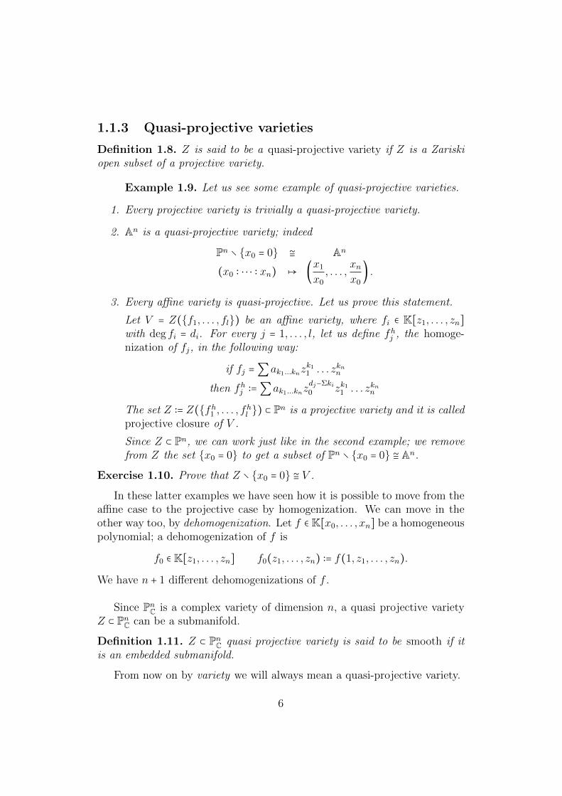
1.1.3 Quasi-projective varieties
Definition 1.8. Z is said to be a quasi-projective variety if Z is a Zariskiopen subset of a projective variety.
Example 1.9. Let us see some example of quasi-projective varieties.
1. Every projective variety is trivially a quasi-projective variety.
2. An is a quasi-projective variety; indeed
Pn ∖ x0 = 0 ≅ An
(x0 ∶ ⋅ ⋅ ⋅ ∶ xn) ↦ (x1
x0
, . . . ,xnx0
) .
3. Every affine variety is quasi-projective. Let us prove this statement.
Let V = Z(f1, . . . , fl) be an affine variety, where fi ∈ K[z1, . . . , zn]with deg fi = di. For every j = 1, . . . , l, let us define fhj , the homoge-nization of fj, in the following way:
if fj =∑ak1...knzk11 . . . zknn
then fhj ∶=∑ak1...knzdj−Σki0 zk11 . . . zknn
The set Z ∶= Z(fh1 , . . . , fhl ) ⊂ Pn is a projective variety and it is calledprojective closure of V .
Since Z ⊂ Pn, we can work just like in the second example; we removefrom Z the set x0 = 0 to get a subset of Pn ∖ x0 = 0 ≅ An.
Exercise 1.10. Prove that Z ∖ x0 = 0 ≅ V .
In these latter examples we have seen how it is possible to move from theaffine case to the projective case by homogenization. We can move in theother way too, by dehomogenization. Let f ∈ K[x0, . . . , xn] be a homogeneouspolynomial; a dehomogenization of f is
f0 ∈ K[z1, . . . , zn] f0(z1, . . . , zn) ∶= f(1, z1, . . . , zn).
We have n + 1 different dehomogenizations of f .
Since PnC is a complex variety of dimension n, a quasi projective varietyZ ⊂ PnC can be a submanifold.
Definition 1.11. Z ⊂ PnC quasi projective variety is said to be smooth if itis an embedded submanifold.
From now on by variety we will always mean a quasi-projective variety.
6

1.1.4 Maps
Definition 1.12. Let X, Y be two varieties; f ∶X → Y is said to be regular(or a morphism of varieties) if
∀x ∈X ∃ U(x) Zariski open, U ⊂ An
V (f(x)) Zariski open, V ⊂ Am
such that f(U) ⊂ V and f ∣U = (g1, . . . , gm) with
gi =nidi, ni, di ∈ K[x1, . . . , xn]
and di(p) ≠ 0 ∀p ∈ U ∀i = 1, . . . ,m.
Basically this means that locally a morphism of algebraic varieties can beexpressed by rational functions.
Definition 1.13. Let X and Y be two quasi-projective varieties; f ∶ X → Yis said to be biregular if it is regular, invertible and with regular inverse.
In algebraic geometry biregular mappings play the role of the diffeomor-phisms in differential geometry and homeomorphisms in topology; that is, ifthere exists a biregular map between two algebraic varieties, it means thatthey look like the same.
Definition 1.14. Let X and Y be two quasi-projective varieties, a rationalmap f ∶ X Y is the equivalence class of pair (U, fU) where U is Zariskiopen, fU ∶ U → Y is regular, modulo the equivalence relation
(U, fU) ∼ (U ′, fU ′)⇔ fU ∣U∩U ′ = fU ′ ∣U∩U ′ .
Example 1.15. Let us see an example of a biregular mapping.Let us define Q ∶= x0x2 = x2
11⊂ P2 and the map
F ∶ P1 → Q(t0 ∶ t1) ↦ (t20 ∶ t0t1 ∶ t21)
.
It is easy to see that this map is well defined (the things to check are thatF (P1) ⊂ Q, that F (λt0, λt1) = F (t0, t1) and that no points are mapped into(0 ∶ 0 ∶ 0) that is not a point of P2).
1With a slight abuse of notation, by this we mean that Q = Z(x0x2 − x21).
7

Let us prove that this is a regular map. Let x = (t0 ∶ t1) ∈ P1 and supposethat t0 ≠ 0, hence x = (1 ∶ t1); in order to satisfy the conditions of Definition1.12, we can define
U(x) = U0 ∶= (t0 ∶ t1) ∈ P1 ∶ t0 ≠ 0V (f(x)) = V0 ∶= (z0 ∶ z1 ∶ z2) ∈ Q ∶ z0 ≠ 0.
U and V are Zariski open subsets of the respective projective subspaces. Re-stricting F to U we get
F ∣U ∶ (1 ∶ t)↦ (1 ∶ t ∶ t2).
Working in an analogous way for point with t0 = 0 and t1 ≠ 0, we get that Fis locally defined by rational functions, hence it is a regular map.
Is this map invertible? Let us then consider the map
G ∶ Q → P1
(x0 ∶ x1 ∶ x2) ↦ (x1
x2
∶ 1)
Apparently, this function is defined only for x2 ≠ 0; but
(x1
x2
∶ 1) = (1 ∶ x2
x1
) ,
thus, G can be equivalently defined for x1 ≠ 0 as
G(x0 ∶ x1 ∶ x2) = (1 ∶ x2
x1
) .
We are still missing the point p = (0 ∶ 0 ∶ 1) ∈ Q; is it possible to define G inan open neighbourhood of p? Exploiting the fact that in Q x0x2 = x2
1 we get
(x1
x2
∶ 1) = (x21
x2
∶ x1) = (x0x2
x2
∶ x1) = (x0 ∶ x1) = (1 ∶ x1
x0
) .
We have then defined the function G over the whole Q.
Exercise 1.16. Prove that G is rational and that G = F −1. Thus F is abiregular mapping.
Remark 1.17. The projection map
π ∶ P2 P1
(x0 ∶ x1 ∶ x2) ↦ (x0 ∶ x1)
8

is a rational map, in the sense that its restriction to the open set P2 ∖ (0 ∶ 0 ∶ 1)is a regular map. Moreover it’s immediate to see that π = G in the commondomain; but π cannot be defined in p = (0 ∶ 0 ∶ 1), whereas G is. This is dueto the fact that restricting the function to Q the limit
limz→pz∈Q
π(z) = (0 ∶ 1)
exists, whilelimz→p π(z)
does not exist.
Exercise 1.18. Let l ∶= ax0 + bx1 = 0 ⊂ P2 with a, b ∈ C; compute using thestandard topology limz→p π∣l and prove that it depends on a, b.
Definition 1.19. A rational map F ∶X Y is said to be birational if thereexists a rational map G ∶ Y X such that F G = IdY and G F = IdX .
If X and Y are two varieties such that there exists a birational mapF ∶X Y , then they are said to be birational.
Definition 1.20. Let X be a variety; X is rational if it is birational to aprojective space.
Definition 1.21. Let X be a variety; X is unirational if it is dominated bya projective space, i.e. there exists a rational map from a projective space toX with dense image.
1.2 Cartier divisors
In this section we introduce the Cartier divisors; the formal definition givesrise to objects that seem quite different from the divisors that are concretelyused. In order to become familiar with divisors, let us first see a concreteexample and then, just after the formal definition, we will see how the firstcorresponds to the latter.
Example 1.22. Let us consider the function
F ∶ P2 C
(x0 ∶ x1 ∶ x2) ↦ x0x21
x2(x0x2 − x21)
The function F is well defined wherever it is defined (since it is the ratio oftwo homogeneous polynomials of the same degree). This function naturallydefines four curves:
9

l0 ∶= x0 = 0l1 ∶= x1 = 0l2 ∶= x2 = 0Q ∶= x0x2 − x2
1.
We say that the divisor of F is
(F ) = l0 + 2l1 − l2 −Q.
Formally, we are describing the zeroes and the poles of F by considering thezero locus of F and 1/F with suitable coefficients:
• l0 has coefficient 1, since F vanishes with multiplicity 1 along it;
• l1 has coefficient 2, since F vanishes with multiplicity 2 along it;
• both l2 and Q have coefficient −1, since F has simple poles along bothof them.
Definition 1.23. Let X be a quasi-projective variety; a (Cartier) divisorover X is a collection (Ui, fi) where:
• Ui is an (affine) open cover of X;
• fi ∶ Ui C are such that ∀i, j
fi/fj ∶ Ui ∩Uj → C
is regular.
The second condition implies that fi/fj(p) ≠ 0 ∀p ∈ Ui ∩ Uj, otherwisefj/fi would not be regular.
We say that two divisors A = (Ui, fi) and B = (Vi, gi) are equivalentif and only if A ∪ B is still a divisor.
Let us see now by an example how these objects can be represented by aformal sum of subvarieties with suitable integer coefficients.
10

Example 1.24. Let Ui ∶= xi ≠ 0 ⊂ P2 and let us define the followingfunctions:
f0 ∶ U0 → C f0 (x1
x0
,x2
x0
) = x2
x0
− (x1
x0
)2
;
f1 ∶ U1 → C f1 (x0
x1
,x2
x1
) = x0
x1
x2
x1
− 1;
f2 ∶ U2 → C f2 (x0
x2
,x1
x2
) = x0
x2
− (x1
x2
)2
.
It’s immediate to see that
fifj
=x2j
x2i
∶ Ui ∩Uj → C
are regular functions, so (Ui, fi) is a divisor. The name we give to this divi-sor is Q = x0x2−x2
1 = 0; indeed, it is immediate to see that, if q = x0x2 − x21,
we havef0 =
q
x20
, f1 =q
x21
, f2 =q
x22
,
thus the curve x0x2 − x21 = 0 coincides locally with the zero locus of the
functions fi.
We will never give a Cartier divisor via a collection (Ui, fi), but al-ways describing its zero locus and the set of its poles with a formal sum ofsubvarieties with integer coefficients: indeed, we will write
D =∑i∈IaiDi,
where ai ∈ Z, every Di is an irreducible variety that can locally be expressedas zero locus of a unique regular function2 and
• D has zeroes of order ai along Di if ai > 0;
• D has poles of order −ai along Di if ai < 0.
The divisor D is said to be effective if ai ≥ 0 ∀i.2Be aware that not all subvarieties are Cartier divisor, but only the subvarieties which
can be locally defined as zero locus of a single rational function.The simplest example is the origin in A2: this is not a Cartier divisor, since we cannotdescribe it using a single function, since its ideal is not principal but needs at least twogenerators. The following exercise give a different and more interesting example.
11

Exercise 1.25. Consider the following affine varieties in C3:
C ∶= Z(y2 − xz), L ∶= Z(x, y);
obviously L ⊂ C. Show that L is not a Cartier divisor in C, but L ∖ O isa Cartier divisor in C ∖ O, where O is the origin of A3.
The set of Cartier divisors over a quasi-projective variety X is an abeliangroup and will be denoted by Div(X).
Example 1.26. When X is a smooth variety of dimension 1
Div(X) = ∑aipi ∶ pi ∈X .
In this particular case if D = ∑aipi ∈ Div(X) we define the degree of D tobe the integer
deg(D) =∑ai.
Definition 1.27. If D ∈ Div(X) is such that D = (F ) for some F ∶ X C,we say that D is a principal divisor.
Remark 1.28. The divisor defined in Example 1.22 is principal, whereas thedivisor Q defined in Example 1.24 is not principal.
Exercise 1.29. Show that Q is not principal. [Hint: ”restrict Q to a line”,and use the well known fact that principal divisors on smooth varieties ofdimension 1 have degree 0.]
Definition 1.30. Let X be a quasi-projective variety and let D1,D2 ∈ Div(X).We say that D1 and D2 are equivalent (denoted by D1 ≡ D2) if and only ifD1 −D2 is a principal divisor.
The Picard group of X is
Pic(X) ∶= Div(X)/ ≡ .
Let us see some example of Picard groups.
Example 1.31. Let X = Pn. Let p0, p1 ∈ C[x0, . . . , xn] two homogeneouspolynomials of the same degree, then
p0
p1
∶ Pn → C
is a rational function. Let Di = pi = 0, then
D0 −D1 = (p0
p1
) .
12
Hence D0 ≡ D1. It can be proved that Pic(Pn) ≅ Z, and the isomorphism isgiven by
Pic(Pn) → Z[∑aiDi] ↦ ∑ai degDi
,
where degDi is the degree of the polynomial that defines the curve Di.
Example 1.32. Let X = P1 × P1. First, let us prove that X is a projectivevariety. Let us define the function
ϕ ∶ P1 × P1 P3
((t0 ∶ t1), (s0 ∶ s1)) ↦ (t0s0 ∶ t0s1 ∶ t1s0 ∶ t1s1)
It’s easy to see that this function is well defined; moreover, denoting with(x0 ∶ x1 ∶ x2 ∶ x3) the homogeneous coordinates of P3, ϕ gives an isomorphismbetween P1 × P1 and Q = x0x3 − x1x2 = 0 ⊂ P3, hence P1 × P1 is a projectivevariety.
It can be proved that Pic(P1 × P1) ≅ Z × Z. If a, b ≥ 0, the isomorphismmaps (a, b) ∈ Z × Z to the class of effective divisors given by bihomogeneouspolynomials with bidegree (a, b) in C[t0, t1][s0, s1], that is polynomials of theform
p =∑λαβta−α0 tα1 s
b−β0 sβ1 .
Exercise 1.33. Prove that Pk1 × ⋅ ⋅ ⋅ × Pkr is a projective variety.
Example 1.34. Let T = C2/Λ be a complex torus, where Λ is a lattice, thatis the subgroup (respect to the sum) generated by two complex numbers whichare linearly independent over R. Being the quotient of a group by a subgroup,T is a group; we know that T can be embedded in P2 as algebraic variety. Itis possible to prove that Pic(T ) ≅ T ×Z and the isomorphism is given by
Pic(T ) → T ×Z[∑aipi] ↦ (∑pi,∑ai)
.
1.3 Sheaves
Definition 1.35. Let X be a topological space, a presheaf of rings (groups,abelian groups, modules,. . . ) F on X is a collection of rings (respectively,of groups, abelian groups, modules, . . . ) F(U) = Γ(U,F) = H0(U,F), onefor every open set U , and a collection of rings (respectively groups, abeliangroups, modules, . . . ) morphisms ρUV ∶ F(U)→ F(V ) whenever V ⊆ U , calledrestriction maps, such that
• F(∅) = 0;
13

• ρUU = IdF(U)∀U ;
• ∀ W ⊂ V ⊂ U ρUW = ρVW ρUV .
An element s ∈ F(U) is called section of F over U . An element of H0(F) ∶=H0(X,F) is called a global section of F .
Example 1.36. Fix a ring G and define the presheaf GX as
GX(U) ∶= f ∶ U → G ρUV (f) = f ∣V .
Example 1.37. The following are presheaves:
Continuous C-valued functions on a topological space C0X
Smooth R-valued functions on a real manifold C∞XHolomorphic C-valued functions on a complex manifold hOXRegular C-valued functions on a variety OXZ-valued constant functions on a topological space ZQ-valued constant functions on a topological space QR-valued constant functions on a topological space RC-valued constant functions on a topological space C
in every case, with the only exception of the fourth one, we use the standardtopology. For OX we use Zariski topology.
Definition 1.38. A presheaf F over X is said to be a sheaf if it satisfies theso called sheaf axiom:
∀U ⊂ X open set, ∀Ui open covering of U , suppose that are given
∀i si ∈ F(Ui) such that ∀i, j ρUi
Ui∩Ujsi = ρ
Uj
Ui∩Ujsj. Then there exists a unique
s ∈ F(U) such that ρUUis = si ∀i.
Basically we are asking that whenever two sections s1 ∈ F(U) and s2 ∈F(V ) agree on the common domain, there exists a unique section s ∈ F(U ∪V ) whose restrictions to U and V are exactly s1 and s2.
Remark 1.39. All presheaves in 1.37 but Z, Q, R, C are sheaves, whileconstant presheaves are not (take into account - for example - two open dis-joint sets). We will consider instead the locally constant functions; in thisway we get the locally constant sheaves Z, Q, R, C.
Example 1.40. The following are sheaves of abelian groups on a smoothvariety:
O∗X = f ∶X → C∗ regular
hO∗X = f ∶X → C∗ holomorphic,
where the group action is given by the multiplication on C∗.
14

Definition 1.41. Let X be a variety and D ∈ Div(X), D = ∑aiDi. Forevery Zariski open set U let us define the complex vector space
Γ(U,OX(D)) ∶= f ∶ U C ∶ (f) +D∣U ≥ 0 ∪ 0;
we will also denote it by H0(U,OX(D)). The set H0(X,OX(D)) will besimply denoted by H0(OX(D)).
Using the same notation of the previous definition, if f ∈ H0(OX(D)),then
• if ai < 0, f vanishes along Di with order at least −ai;
• if ai > 0, f admits poles over Di of order up to ai.
f is a rational function with a principal divisor (f). Anyway, when consid-ering it as a section of OX(D) we will usually denote it by the letter s (torecall that we are not considering it as a function) and attributes to it theeffective divisor (s) ∶= (f) +D.
Using this notation, it is possible to prove that
(s1) = (s2)⇔ ∃λ ∈ C∗ ∶ s1 = λs2. (1.2)
The dimension of H0(OX(D)) will be denoted by
h0(OX(D)) ∶= dimH0(OX(D)).
Proposition 1.42. If D1,D2 ∈ Div(X) are linearly equivalent, then H0(OX(D1)) ≅H0(OX(D2)) via an isomorphism that preserves the divisors. In other words,if s1 ∈H0(OX(D1)) is mapped by this isomorphism to s2 ∈H0(OX(D2)), then(s1) = (s2).
Proof. D1 ≡ D2 ⇔ D1 −D2 = (F ) with F ∶ X C. If f ∈ H0(U,OX(D1)),then
(fF ∣U) = (f) + (F ) = (f) +D1 −D2 ≥ −D2,
hence fF ∣U ∈H0(U,OX(D2)). The sheaves isomorphism is given by
H0(U,OX(D1)) → H0(U,OX(D2))f ↦ fF ∣U
g/F ∣U g
Let us prove the second part of the statement: the divisor of f as a sectionof H0(OX(D1)) is (f) +D1, while the divisor of its image is (fF ) +D2 =(f) + (F ) +D2 = (f) +D1 −D2 +D2 = (f) +D1.
15

Example 1.43. Let X = P2, L0 = x0 = 0, L1 = x1 = 0; by Example1.31, L0 ≡ L1, hence, by Proposition 1.42, H0(OX(L1)) ≅ H0(OX(L2)); letf ∈H0(O(L0)), then f = L/x0, where L ∈ C[x0, x1, x2]1.
It is immediate to see that the isomorphism defined in Proposition 1.42maps f into g = L/x1; the divisor we get is (f) + L0 equal to (g) + L1 equalto (s) = L = 0.
By (1.2) the set
∣D∣ ∶= (s) ∶ s ∈H0(OX(D)), s ≠ 0
is a subset of Div(X) formed by effective divisors having a natural structureof projective space, indeed ∣D∣ ≅ Ph0(OX(D))−1. The set ∣D∣ is called completelinear system associated with D and gives exactly those effective divisorswhich are linearly equivalent to D. A linear system is a linear subspace of acomplete linear system.
Exercise 1.44. All rational functions on Pn can be obtained by taking thequotient of two homogeneous polynomial of the same degree (we are not askingyou to prove it, take it as true).
Let D be a (non necessarily effective) divisor on Pn and let d ∈ Z its degree(i.e. its class in Pic(Pn)). Give an explicit isomorphism among H0(O(D))and the vector space of the homogeneous polynomials of degree d.
Exercise 1.45. State and solve an exercise similar to the previous one, butconsidering P1×P1 instead of Pn. Here you will need that every rational func-tion on P1 × P1 can be obtained by taking the quotient of two bihomogeneouspolynomials of the same bidegree.
1.4 Pull-back and push-forward
Definition 1.46. Let X and S be two varieties and f ∶X → S a morphism;let D ∈ Div(S), D = ∑aiDi. We define the pull-back of D f∗D ∈ Div(X) as
f∗D ∶=∑aif∗Di,
where, if Di is locally defined by fi, f∗Di is locally defined by fi f .
Example 1.47. Let
f ∶ P1 → P1
(x0 ∶ x1) ↦ (x20 ∶ x2
1)
and let us consider P1 ∶= (1 ∶ 0), P2 ∶= (1 ∶ 1), P3 ∶= (1 ∶ −1). Then
f∗(P2) = P2 + P3, f∗(P1) = 2P1.
16

Remark 1.48. Using the same notation of previous definition, the followingfacts hold:
1. D effective ⇒ f∗D is effective;
2. D1 ≡D2 ⇒D1−D2 = (g) for some g ∶ S C⇒ f∗D1−f∗D2 = (gf)⇒f∗D1 ≡ f∗D2;
3. f∗ ∶ Div(S)→ Div(X) is a homomorphism of abelian groups; since, by2., the subgroup of principal divisors of S is mapped into the subgroupof principal divisors of X, f∗ induces a homomorphism
f∗ ∶ Pic(S) → Pic(X)[D] ↦ [f∗D] .
The definition of pull-back is natural. The next definition, the push-forward, needs some extra assumptions.
Definition 1.49. Let X be a smooth surface (i.e. a complex variety ofdimension 2). Let f ∶ X → S be a generically finite map of degree d, that is∃U ⊂ S open set such that ∀p ∈ U #f−1(p) = d.
If D = ∑aiDi ∈ Div(X), then the push-forward of D is f∗D ∶= ∑aif∗Di ∈Div(S), where
• if f(Di) is constant, then f∗Di ∶= 0 ∈ Div(S);
• otherwise f(Di) is a Cartier divisor in S and Di → f(Di) is genericallyfinite of degree r ≤ d. In this case we define f∗Di ∶= rf(Di).
Remark 1.50. Using the notation of previous definition, the following factshold:
1. D effective ⇒ f∗D is effective;
2. D1 ≡D2 ⇒ f∗D1 ≡ f∗D2;
3. f∗ ∶ Div(X)→ Div(S) is a homomorphism of abelian groups, hence, asin the case of pull-back, f∗ induces a homomorphism f∗ ∶ Pic(X)→ Pic(S);
4. f∗f∗D ≡ dD.
Example 1.51. Let
g ∶ P2 → P2
(x0 ∶ x1 ∶ x2) ↦ (x20 ∶ x2
1 ∶ x22).
17

This map is generally finite of degree 4.Let us consider l0 ∶= x0 = 0 ∈ Div(P2), then it is easy to see that
g∗l0 = 2l0. Moreover, g(l0) = l0 and g∣l0 ∶ l0 → l0 has degree 2, hence g∗l0 = 2l0.Eventually, it is immediate to see that g∗g∗l0 = 4l0.
Let us now consider l = x0 + x1 + x2 = 0 ∈ Div(P2); first of all, weobserve that l ≡ l0, hence, by Remark 1.50, we expect g∗l ≡ g∗l0 = 2l0. Indeedg(l) = x2
0 + x21 + x2
2 − 2x0x1 − 2x0x2 − 2x1x2 = 0 and that g∣l ∶ l → g(l) hasdegree 1. Hence g∗l = g(l) ≡ 2l0.
1.5 Intersection multiplicity
From now on by surface we will always mean a smooth variety of dimension2 and by curve in it an irreducible divisor in it.
Let S be a surface and C,C ′ curves in it with C ≠ C ′. ∀x ∈ S we definethe set
Ox ∶= germ in x of regular functions f ∶ U → C, x ∈ U;
this set is called local ring of S at x.
Definition 1.52. Let x ∈ C ∩C ′ and f, g ∈ Ox germs of regular functions atx that define C and C ′ respectively. We define the intersection multiplicityof C and C ′ at x as
mx(C,C ′) ∶= dimCOx/(f, g)
Remark 1.53. By Hilbert Nullstellensatz mx(C,C ′) <∞.
Example 1.54. Let S = C2, C = x = 0, C ′ = y = 0, p = 0. Then the map
Op/(x, y) → C[f] ↦ f(0)
is an isomorphism. Therefore mp(C,C ′) = 1.
Following propositions are given without proof.
Remark 1.55. Under the hypotheses of Definition 1.52, ∀x ∈ C∩C ′, mx(C,C ′) ≥1.
The following proposition, which we do not have time to prove, gives aclear interpretation of the intersection multiplicity.
18

Proposition 1.56. Under the hypotheses of Definition 1.52, mx(C,C ′) =1⇔ both C and C ′ are smooth in x and intersect transversely.
Exercise 1.57. Using the same notation of Example 1.54, prove that
mp(x = 0,x = yr) = r;mp(x = 0,x2 = y3) = 3;
mp(y = 0,x2 = y3) = 2.
Definition 1.58. Under the hypotheses of Definition 1.52 we define the in-tersection number of C and C ′ as
C ⋅C ′ ∶= ∑x∈C∩C′
mx(C,C ′). (1.3)
By Hilbert Nullstellensatz the sum in (1.3) is finite, hence C ⋅C ′ <∞.
1.6 Morphisms of sheaves
Definition 1.59. Let X be a variety and let F ,G be two sheaves of rings(groups,. . . ). A function
f ∶ F → G
is said to be a morphism of sheaves if ∀U ⊂X open set fU ∶ F(U)→ G(U) isa ring (group,. . . ) homomorphism, and ∀U,V ⊂X open sets such that V ⊂ U ,the diagram
F(U) fUÐÐÐ→ G(U)
ρUV
×××Ö×××ÖρUV
F(V ) ÐÐÐ→fV
G(V )
commutes.
Example 1.60. Let us see some fundamental examples of morphisms ofsheaves.
1. Let D1,D2 ∈ Div(X) such that D1 ≡ D2, then D1 −D2 = (F ) for someF ∶X C; then ∀U open set we define the morphism
Γ(U,OX(D1)) → Γ(U,OX(D2))f ↦ fF ∣U
;
these maps give a morphism of sheaves among OX(D1) and OX(D2).
19

2. Let Y be a variety and X ⊂ Y a subvariety; the restriction
OY → OX
is a morphism; actually, we cannot give a morphism among two sheavesdefined on different varieties, but we can see OX as a sheaf on Y defin-ing ∀U ⊂ Y Zariski open set Γ(U,OX) ∶= Γ(U ∩X,OX).
3. Let C,D ∈ Div(X), with C irreducible, D = ∑aiDi with C ≠ Di ∀i.
Under these hypotheses, the divisorD∣C ∈ Div(C) is well defined: if locallyDi = (fi), then Di∣C = (fi∣C).The restriction
OX(D)→ OC(D∣C)
is a morphism of sheaves if we con-sider the latter as sheaf on X as inthe previous case.
4. C,D ∈ Div(X), D ≥ 0. Let U ⊂ X be an open set; if f ∈ Γ(U,OX(C)),then (f)+C ≥ 0, thus (f)+C+D ≥D ≥ 0. This means that f ∈ Γ(U,OX(C +D)).The function
OX(C) → OX(C +D)f ↦ f
is well defined and is a morphism.
Definition 1.61. Let F ,G be two sheaves on X and let f ∶ F → G be amorphism of sheaves. ∀U ⊂X open set we define
(kerf)(U) ∶= u ∈ F(U) ∶ fU(u) = 0 ⊂ F(U).
Exercise 1.62. ker f is a sheaf.
Definition 1.63. A morphism of sheaves f ∶ F → G is said to be injective ifker f = 0⇔ ∀U ker fU = 0.
Remark 1.64. The morphisms defined in Examples 1.60.1 and 1.60.4 areinjective.
Definition 1.65. Let F ,G be two sheaves on X and f ∶ F → G a morphismof sheaves; f is said to be surjective if ∀p ∈ X ∃U ⊂ X open set p ∈ Usuch that ∀ξ ∈ G(U) ∃V ⊂ U open set with p ∈ V and ∃η ∈ F(V ) such thatfV (η) = ρUV (ξ).
20

Remark 1.66. The morphisms defined in Examples 1.60.1, 1.60.2 and 1.60.3are surjective.
Exercise 1.67. The function
exp ∶ hOC → hO∗C
f ↦ e2πif
is a morphism of sheaves of abelian group (where the operation on hOC isthe sum, while the operation on hO∗
C is the multiplication). This morphismis surjective, but it is not surjective on C∗ since the function z (the identity)gives a section of Γ(C∗,hOC∗), which is not of the form e2πif : indeed mostcourses in complex analysis show that log z cannot be defined on the wholeC∗.
Definition 1.68. An injective and surjective morphism of sheaves is calledisomorphism of sheaves.
By the previous remarks, D1 ≡D2 ⇒ OX(D1) ≅ OX(D2).
Definition 1.69. Let A, B, C be three sheaves on X; we say that
0→ A fÐ→ B gÐ→ C → 0
is a short exact sequence of sheaves if
• g is a surjective morphism;
• f is an injective morphism;
• f(A) ⊂ ker(g) and f ∶ A→ ker(g) is surjective.
Definition 1.70. A sequence of morphisms of sheaves
. . .Ð→ Ai−1fiÐ→ Ai
fi+1Ð→ Ai+1 Ð→ . . .
is said to be exact if fi surjects to kerfi+1 ∀i.
Exercise 1.71. Let S be a variety; ∀C irreducible divisor in S and ∀D ∈Div(S) there are exact sequences.
0→ OS(−C)Ð→ OS Ð→ OC → 0
and0→ OS(D −C)Ð→ OS(D)Ð→ OC(D)→ 0
21

1.7 Cech cohomology
Definition 1.72. Let F be a sheaf on X; ∀U ⊂X open set, ∀q ∈ N ∃ Hq(F)q-th Cech cohomology group such that:
1. H0(F) = Γ(X,F);
2. ∀0 → A → B → C → 0 short exact sequence of sheaves ∃ a long exactsequence of cohomology groups
0→ H0(A)→ H0(B)→ H0(C)→ H1(A)→ H1(B)→ H1(C)→ . . .(1.4)
3. If F is a coherent sheaf of OX−modules and X is projective, then allHq(F) are C-vector spaces of finite dimension and each map in (1.4)is linear;
4. Under the hypotheses of previous point, if dimX = n, then Hq(F) = 0∀q > n (if X is not smooth, then there exists a Zariski open set U ⊂ Xsmooth; in this case dimX ∶= dimU).
Definition 1.73. Under the hypotheses of the last point of Definition 1.72,the Euler-Poincare characteristic of F is
χ(F) ∶=∑ (−1)qhq(F),
where hq(F) ∶= dim Hq(F).
Exercise 1.74. If 0 → A → B → C → 0 is a short exact sequence ofOX-modules, then χ(A) + χ(C) = χ(B).
1.8 The Canonical sheaf
Definition 1.75. Let X be a variety of dimension n; by ΩqX we denote the
sheaf of regular q-form on X, that is
ΩqX(U) ∶= ω ∶ locally ω = ∑
1≤i1≤⋅⋅⋅≤iq≤nfi1...iqdxi1 ∧ ⋅ ⋅ ⋅ ∧ dxiq ,
where xi are regular local coordinates and fi1...iq are regular
ΩnX is called canonical sheaf.
Let ω ∈ ΩnX(U), then locally ω = fdx1∧⋅ ⋅ ⋅∧dxn is defined through a single
rational function f . Hence the locus of zeroes and poles of ω, locally definedas the locus of zeroes and poles of f , is a Cartier divisor.
22

Definition 1.76. Let ω be a rational n−form on X so regular on a Zariskiopen subset of X, then (ω) is defined as the divisor of its zeroes and poles.A divisor of this kind is said to be canonical.
Remark 1.77. Let ω be a rational n−form on X and g a rational functionon X, then gω is another rational n−form and its Cartier divisor is (gω) =(g)+ (ω)⇒ (ω) ≡ (gω). In other words every divisor linearly equivalent to acanonical divisor is still a canonical divisor.
Vice versa, suppose that ω′ is another rational n−form, write locally ω =fdx1 ∧ ⋅ ⋅ ⋅ ∧ dxn and ω′ = f ′dx1 ∧ ⋅ ⋅ ⋅ ∧ dxn, then f ′/f does not depend on thecoordinates and therefore defines a rational function on X. 3 This impliesthat (ω) ≡ (ω′), that is the canonical divisors form an equivalence class forthe relation ”linear equivalence”. This equivalence class is then an elementof Pic(X), usually denoted by K (sometimes we will denote - with a slightabuse of notation - by K any canonical divisor in Div(X)).
Example 1.78. Let X = P1 and consider the usual open sets
U0 ∶= x0 ≠ 0 with local coordinate x = x1/x0
U1 ∶= x1 ≠ 0 with local coordinate y = x0/x1.
It is immediate to see that in U0 ∩U1 y = 1/x.Let us consider ω ∈ Ω1
X(U0) defined as ω = dx. As a rational 1−form onX it has no zeroes and a double pole in (0 ∶ 1) since in the coordinates of U1:
ω = d(1
y) = −dy
y2.
Hence (ω) = −2P . As we saw in a previous section, Pic(P1) ≅ Z, henceKP1 = −2.
Exercise 1.79. Prove that:
1. KPn = −(n + 1) < 0;
2. KP1×P1 = (−2,−2).
Remark 1.80. By Exercise 1.79 and Exercise 1.44, it is immediate to seethat H0(KPn) = 0, since there are no homogeneous polynomials of degree< 0.
3By a slight abuse of notation we could write that ωω′
is a rational function.
23

Exercise 1.81. Let K = (ω) ∈ Div(X) with ω rational n−form. Prove that
O(K) Ð→ ΩnX
f z→ fω
is an isomorphism of sheaves.
We do not prove the next two statements.
Theorem 1.82. Let C be a smooth compact curve (that is a Riemann sur-face) ⇒ h0(Ω1
C) = g, where g is the genus of C.
Theorem 1.83 (Serre duality). Let X be a smooth variety of dimension n,then ∀q,∀D ∈ Div(X)
Hq(D) ≅Hn−q(K −D)∗.
Remark 1.84. Let C be a smooth compact curve. We have seen that
hq(OC) = 0 if q ≠ 0,1;
h0(OC) = 1;
h1(OC) = h0(KC) = g;
hence χ(OC) = 1 − g.
Definition 1.85. Let X be a variety, p1, . . . , pr ∈ X. A skyscraper sheafsupported on p1, . . . , pr is a sheaf F obtained by associating to each pi avector space Vi and then by taking ∀U ⊂X open set
F(U) = ⊕i∶pi∈U
Vi
with the natural restrictions.
By the definition of Cech cohomology, it is easy to prove the following
Proposition 1.86. Using the same notation of the previous definition, H0(F) ≅⊕Vi and ∀q ≠ 0 hq(F) = 0.
Example 1.87. Let X be a variety p ∈ X, then Op ≅ C, seen as a sheaf onX (as we did in Example 1.60.2), is a skyscraper sheaf supported on p.
More generally, ∀Y ⊂ X, if F is a sheaf on Y , then Hq(F) does notchange if F is considered as a sheaf defined on X.
24
1.9 Riemann-Roch theorem
Let C be a smooth compact curve; let us define for all points p ∈ C theevaluation map at p to be
eval ∶ OC Ð→ Opf z→ f(p) ;
it is immediate to see that
ker(eval) = f regular ∶ f(p) = 0= f regular ∶ (f) − p ≥ 0 = OC(−p),
hence0Ð→ OC(−p)Ð→ OC
evalÐ→ Op Ð→ 0
is an exact sequence.Analogously, ∀D ∈ Div(C) D = ∑aipi such that ∀i p ≠ pi, the sequence
0Ð→ OC(D − p)Ð→ OC(D) evalÐ→ Op Ð→ 0 (1.5)
is exact. Since D ≡ D′ ⇒ OC(D) ≅ OC(D′), and since one can always find adivisor D′ linearly equivalent to D which does not involve a chosen point p,we can drop the hypothesis for which p ≠ pi ∀i (1.5).
Corollary 1.88. ∀p ∈ C, ∀D ∈ Div(C) χ(OC(D)) = χ(OC(D − p)) + 1.
Proof. The sequence 0 → OC(D − p) → OC(D) → Op → 0 is exact. Henceχ(OC(D)) = χ(OC(D − p)) + χ(Op) = χ(OC(D − p)) + 1.
Corollary 1.89. Let C be a smooth compact curve of genus g, then ∀D ∈Div(C)
χ(OC(D)) = deg(D) − g + 1.
Proof. By Corollary 1.88 if the statement is true for a divisor D, then, forevery p, the statement is true both for D − p and D + p. It is then enough toprove it for a divisor, and indeed it is true for D = 0 by Remark 1.84.
This corollary, known as Riemann-Roch theorem, is usually written in adifferent way; indeed, under our hypotheses
χ(OC(D)) = h0(D) − h1(D) = h0(D) − h0(K −D),
where the last equality holds by Serre duality. Hence
h0(D) − h0(K −D) = deg(D) − g + 1.
However, we prefer the statement of Corollary 1.89 since it does generalizeto higher dimensional varieties.
25

1.10 The intersection form
Let S be a smooth projective surface, C,C ′ ∈ Div(S) irreducible and C ≠ C ′;in a previous section, ∀x ∈ C ∩C ′ we have considered the ring
OC∩C′,x ∶= Ox/(s, s′)
where s and s′ are the local equations of C and C ′ respectively. More pre-cisely, we defined the intersection multiplicity of C and C ′ at x as the dimen-sion of it as a complex vector space. We define OC∩C′ to be the skyscrapersheaf supported on C ∩C ′ that associates to each x ∈ C ∩C ′ the ring OC∩C′,x.
Lemma 1.90. Let S be a smooth surface, C,C ′ ∈ Div(S) irreducible andC ≠ C ′, then there exists an exact sequence
0Ð→ OS(−C −C ′) αÐ→ OS(−C)⊕OS(−C ′) βÐ→ OSγÐ→ OC∩C′ Ð→ 0. (1.6)
Proof. Let us define α, β and γ.Map γ ∶ OS → OC∩C′ simply maps f ∈ OS(U) in its classes in each
Ox/(s, s′). This map is trivially surjective.By definition f ∈ kerγ ⇔ ∀x ∈ U [f]Ox ∈ (s, s′), that is if and only if
locally f = as + bs′. Hence, since we want (1.6) to be exact, we define
β(a, b) = as + bs′,
so that β surjects on kerγ. Finally, we define
α(h) = (s′h,−sh).
It is immediate to see that α is injective and that β α = 0. The surjectivityof α onto kerβ follows from standard results of commutative algebra usingthat C and C ′ are irreducible and distinct (this means that s and s′ arerelatively prime).
Now that we have a long exact sequence, we can split it into short exactsequences, and compute χ of the members of such sequences. From (1.6) weget the exact sequences
0Ð→ OS(−C −C ′)Ð→ OS(−C)⊕OS(−C ′)Ð→ kerγ Ð→ 0
0Ð→ kerγ Ð→OS Ð→ OC∩C′ Ð→ 0.(1.7)
We recall that
χ(OC∩C′) = h0(OC∩C′) =∑mx(C,C ′) = C ⋅C ′.
26

From (1.7) and Exercixe 1.74 follows that
C ⋅C ′ = χ(OS) + χ(OS(−C −C ′)) − χ(OS(−C)) − χ(OS(−C ′)). (1.8)
Note that (1.8) gives an expression of C ⋅ C ′ which only depends on theequivalence class of C and C ′ modulo linear equivalence. In particular C ⋅C ′
does not change if we substitute C by a different curve linearly equivalentto it, since the right member of (1.8) depends not on C,C ′ ∈ Div(S) but ontheir classes in Pic(S). This suggests us to use (1.8) to extend the definitionof intersection to a form on Pic(S).
Definition 1.91. ∀D1,D2 ∈ Pic(S) we define
D1 ⋅D2 ∶= χ(OS) + χ(OS(−D1 −D2)) − χ(OS(−D1)) − χ(OS(−D2)). (1.9)
Theorem 1.92. (1.9) defines a symmetric bilinear form on the abelian groupPic(S) such that, if C1 ∈ ∣D1∣, C2 ∈ ∣D2∣ are irreducible and C1 ≠ C2, thenD1 ⋅D2 = C1 ⋅C2 = ∑x∈C1∩C2
mx(C1,C2).
We have already remarked that the last part of the theorem holds, andby definition, it is immediate to see that D1 ⋅D2 = D2 ⋅D1. We need onlyto prove bilinearity. Since the function is defined on an abelian group, bybilinearity we mean
(D +D′) ⋅C = (D ⋅C) + (D′ ⋅C) and D ⋅ (C +C ′) =D ⋅C +D ⋅C ′.
Lemma 1.93. Let C be a smooth curve on S, D ∈ Div(S), then
C ⋅D = degOC(D) = degD∣C .
Proof. The sequences
0Ð→ OS(−C)Ð→ OS Ð→ OC Ð→ 0
0Ð→ OS(−C −D)Ð→ OS(−D)Ð→ OC(−D)Ð→ 0
are exact. Hence using Riemann-Roch on C
C ⋅D = χ(OS) − χ(OS(−C)) − χ(OS(−D)) + χ(OS(−C −D))= χ(OC) − χ(OC(−D))= 1 − g − (1 − g + deg(OC(−D)))= deg(OC(D)).
27

∀D1,D2,D3 ∈ Pic(S) let us define the function
s(D1,D2,D3) ∶= (D1 ⋅ (D2 +D3)) − (D1 ⋅D2) − (D1 ⋅D3).
Exercise 1.94. s(D1,D2,D3) = s(Dσ(1),Dσ(2),Dσ(3)) ∀σ ∈ S3.
By Lemma 1.93, if ∃ C ∈ ∣D1∣ smooth, then
s(D1,D2,D3) = degOC(D2 +D3) − degOC(D2) − degOC(D3) = 0,
since, on a curve deg(A + B) = degA + degB. Hence, by Exercise 1.94, if∃ C ∈ ∣D3∣ smooth, s(D1,D2,D3) = 0.
We can now prove Theorem 1.92.
Proof of Theorem 1.92. Let A,B ∈ Div(S) be smooth and irreducible andD ∈ Div(S), then, since B is smooth,
0 = s(D,A −B,B) = (D ⋅A) − (D ⋅ (A −B)) − (D ⋅B),
thus D ⋅ (A−B) = (D ⋅A)− (D ⋅B) = degD∣A−degD∣B, which in turn impliesthat the map D → D ⋅ (A −B) is linear (and therefore by simmetry also themap D →D ⋅ (B −A)).
The theorem follows then since every divisor is linearly equivalent to adifference of smooth effective divisors, by the classical Theorem of Bertiniand Serre which we recall immediately after this proof.
Definition 1.95. Let X be a variety; D ∈ Div(X) is said to be very ample if∃ an embedding of X in Pn such that D is the Cartier divisor locally defined bythe restriction to X of (x0) (equivalently we will say that ”D is a hyperplanesection” or that D =X ∩ x0 = 0).
Exercise 1.96. If D is very ample, then nD is very ample ∀n ∈ N with n ≥ 1.
The two following fundamental theorems will be stated without proof.
Theorem 1.97 (Theorem of Bertini). If X is smooth and D is very ample,then ∃C ∈ ∣D∣ smooth and irreducible.
The geometric idea lying under the theorem of Bertini is that if we cutX with a generic hyperplane, we get a smooth subvariety of X.
Theorem 1.98 (Theorem of Serre). Let X be a variety, A,D ∈ Div(X) withA very ample and D effective; then ∃n0 ∈ N such that ∀n ≥ n0 D+nA is veryample.
28
Let S be a projective variety, ∀C ∈ Div(S) we are interested in computingthe value C2 = C ⋅C. Let us see some examples.
Example 1.99 (Fibered surfaces). Let S be a projective, smooth and irre-ducible surface and let π ∶ S → C be a surjective morphism, with C smoothirreducible curve. ∀p ∈ C p ∈ Div(C), hence we shall consider the pull-backπ∗p = Fp ∈ Div(S), where by Fp we denote the fiber over p.
First, let us remark that there exists ∑aipi ∈ Div(C) such that p ≡ ∑aipiand p ≠ pi ∀i. Since, by Remark 1.48, the pull-back preserve linear equiva-lence,
Fp = π∗p ≡ π∗ (∑aipi) =∑aiπ∗pi =∑aiFpi ,
thusF 2p = Fp ⋅ (∑aiFpi) =∑ai(Fp ⋅ Fpi)
(#)= ∑ai0 = 0,
where equality (#) holds because Fp ∩ Fpi = ∅ ∀i.Example 1.100. Let S = P2, C1 = fd1 = 0, C2 = fd2 = 0, where fdi =C[x0, x1, x2]di (possibly equal). Then C1 ≡ d1l0 and C2 ≡ d2l1; hence
C1 ⋅C2 = (d1l0) ⋅ (d2l1) = d1d2(l0 ⋅ l1) = d1d2,
where last inequality holds because of Proposition 1.56, since l0 ⋔ l1 = (0 ∶ 0 ∶ 1).
Exercise 1.101. Let C1,C2 ∈ Pic(P1 × P1) ≅ Z × Z, with C1 = (a1, b1) andC2 = (a2, b2); compute C1 ⋅C2.
(To check if the solution is right, (2,7)(3,6) = 33)
Theorem 1.102 (Riemann-Roch theorem for surfaces). Let S be a projectivesurface, D ∈ Div(S), then
χ(OS(D)) = χ(OS) +1
2(D2 −DK). (1.10)
Proof. By (1.9)
(−D) ⋅ (D −K) = χ(OS) + χ(OS(K)) − χ(OS(D)) − χ(OS(K −D));
by Serre duality hq(OS(D)) = h2−q(OS(K −D)), hence, since 2 − q is evenwhenever q is, we conclude that χ(OS(D)) = χ(OS(K −D)). Therefore
(−D) ⋅ (D −K) = 2(χ(OS) − χ(OS(D)),
hence
χ(OS(D)) = χ(OS) −1
2(−D)(D −K)
= χ(OS) +1
2D(D −K).
29

Corollary 1.103. Under the hypotheses of Theorem 1.102, if χ(OD) > 0then at least one among ∣D∣ and ∣K −D∣ is non empty.
Proof. h0(D) + h0(K − D) = h0(D) + h2(D) ≥ χ(OS(D)) > 0, where thefirst equality holds by Serre duality. Hence at least one among h0(D) andh0(K −D) is strictly greater than zero.
Corollary 1.104 (Genus formula). Let C be a smooth curve in S, then thegenus of C is
g = 1 + 1
2(C2 +CK).
Proof. Let us consider the exact sequence
0Ð→ OS(−C)Ð→ OS Ð→ OC Ð→ 0.
Henceg = 1 − χ(OC) by Corollary 1.89
= 1 − χ(OS) + χ(OS(−C))= 1 + 1/2((−C)2 − (−C)K) by Theorem 1.102= 1 + 1/2(C2 +CK).
Exercise 1.105. Compute the genus of a smooth plane curve of degree d.
Exercise 1.106. Compute the genus of a curve in P1 ×P1 of bidegree (a, b).
Definition 1.107. If D ∈ Div(S) the arithmetic genus of D is
pa(D) ∶= 1 + 1
2(D2 +DK).
We state the following result without proof.
Theorem 1.108 (Theorem of Noether).
χ(OS) =1
12(K2 + e), (1.11)
where e is the Euler topological characteristic of S (in this particular casee = ∑4
q=0 (−1)qhqDR(S), where H∗DR denotes the De Rham cohomology).
30

Chapter 2
Birational maps
Before beginning a classification, we have to decide when we are going toconsider two of the objects we are classifying to be equivalent. In algebraicgeometry, we classify varieties up to isomorphism or, more coarsely, up tobirational equivalence. The problem does not arise for curves, since a rationalmap from one smooth complete curve to another is in fact a morphism. Forsurfaces, we shall see that the structure of birational maps is very simple;they are composites of elementary birational maps, the blow ups.
2.1 Blow ups
In this section we study a classical example of morphism wich is birationalbut not biregular, called blow up.
Definition 2.1. Let S be a smooth surface and p ∈ S, then there exists asmooth surface S1, called blow up of S in p, and a birational morphismε ∶ S → S such that
1. E ∶= ε−1(p) ≅ P1 (this set is called exceptional divisor);
2. ε∣S∖E ∶ S ∖E Ð→ S ∖ p is biregular.
Example 2.2. To describe explicitly the behaviour of the blow up in a neigh-bourhood of p, it is enough to describe the case of S = C2 in p = (0,0): indeedall blow ups can be obtained by this example writing everything in suitable
1To be precise S exists always as a complex manifold, or as ”algebraic variety” (acomplex manifold with an atlas whose transition functions are regular maps) but notalways as a quasi-projective variety.
31
local coordinates. Let us denote the coordinate on C2 by (x, y) and those onP1 by (t0 ∶ t1). We define
C2 ∶= xt1 = yt0 ⊂ C2 × P1
andε ∶ C2 Ð→ C2
((x, y), (t0 ∶ t1)) z→ (x, y)First of all, it is immediate to see that
ε−1(0) = 0 × P1 ⊂ C2 × P1.
Now let us prove that C2 is smooth.Let p ∈ C2; if t1(p) ≠ 0, then U1 ∶= C2 ∩ t1 ≠ 0 ⊂ C3 with coordinates
x, y, t = t0/t1 and its equation is f = x − yt = 0. Since ∂f/∂x ≠ 0, by the localdiffeomorphism theorem y, t are local coordinates (indeed x = yt). Hence C2
is smooth in p. Note that in this open set E is the divisor of the functiony. If t0 ≠ 0, then in U0 ∶= C2 ∩ t0 ≠ 0 we shall use as local coordinatesx, y, u = t1/t0; analogously to the previous case, the local equation of C2 isg = y − xu, thus x,u are local coordinates and y = xu. Moreover, we shallremark that in the first open set E is the divisor of the function x.
The last thing we have to prove is the second point of Definition 2.1.Basically, it means that ε∣C2∖E is invertible. Indeed
ε∣−1
C2∖E ∶ (x, y)z→ ((x, y), (x ∶ y)).
Definition 2.3. Let C be an effective divisor on S with p ∈ C; locally C =(f), with f(x, y) regular function, where x, y are local coordinates such thatp = (0,0). Then we shall consider the Taylor series of f in a neighbourhoodof p;
f = fm(x, y) + fm+1(x, y) + . . . , where fk ∈ C[x, y]k∀k and fm /≡ 0 ∶
in this case we define the multiplicity of C in p to be equal to m.
Definition 2.4. If C = ∑aiCi ∈ Div(S), the strict transform of C is C =
∑aiCi, where Ci ∶= (ε∣−1S∖E)∗(C − p)
Sis a Cartier divisor in S.
32

Example 2.5. In the situation of Ex-ample 2.2, let us consider
l = (ax + by = 0) ∈ Div(C2),
then
l = (ax + by = at0 + bt1 = 0),
thus l ⋔ E = ((0,0), (−b ∶ a)), thus theintersection point l ∩ E determines abijection among E and the set of thelines through p.More generally the same computationshows that the strict transform C ofevery curve smooth at p is a curveisomorphic to C (through the projec-tion) intersecting E transversally atthe point given by the tangent directionof C at p.
From now on we will assume S and S projective, in order to be able toconsider their intersection forms.
Lemma 2.6. Let C ∈ Div(S) effective and irreducible and suppose that itsmultiplicity in p is m, then
ε∗C = C +mE.
Proof. Clearly ε∗C = αC + βE with α,β ∈ Z (since if locally C = (f), thenε∗C = (ε∗f) = (f ε) and ε−1C = C ∪E). Since ε is biregular out of p, thenα = 1 (multiplicity cannot change because of biregularity).
Now, let us assume that locally C = (f) for some f(x, y) rational function,where x, y are local coordinates such that p = (0,0). Then
f = fm(x, y) + fm+1(x, y) + . . . , where fk ∈ C[x, y]k∀k and fm /≡ 0.
In an open neighbourhood of q ∈ E with t1(q) ≠ 0 we have local coordinatesy, t and x = yt, so
ε∗f = fm(yt, y) + fm+1(yt, y) + . . .= ymfm(t,1) + ym+1fm+1(t,1) + . . .= ym[fm(t,1) + yfm+1(t,1) + . . . ]
Hence ε∗f vanishes with multiplicity m in E = (y), thus β =m.
33

Proposition 2.7. The following properties hold:
1. The mapPic(S)⊕Z Ð→ Pic(S)
(C,n) z→ ε∗C + nEis a group isomorphism.
2. ∀D,D′ ∈ Pic(S)
ε∗D ⋅ ε∗D′ =D ⋅D′;E ⋅ ε∗D = 0;
E2 = −1.
3. KS = ε∗KS +E.
Proof. 2. Since ε is biregular out of p, it is generically finite of degree 1and therefore ε∗D ⋅ ε∗D′ =D ⋅D′. By the Theorem of Serre and Bertinievery divisor is linearly equivalent to a divisor involving only curvesnot containing p, then Supp(ε∗D) ∩E = ∅, hence E ⋅ ε∗D = 0.
Let C smooth in p with multiplicity 1 in p. Then ε∗C = C + E byLemma 2.6; moreover, using local coordinate, we get C ⋅E = 1. Then
0 = E ⋅ ε∗C = E ⋅ (C +E) = E ⋅ C +E2 = 1 +E2.
Hence E2 = −1.
1. Injectivity: Suppose ε∗D + nE = 0⇒ 0 = E(ε∗D + nE) = 0 − n⇒ n = 0.Hence ε∗D ≡ 0, thus, D = ε∗ε∗D = ε∗0 = 0, where the first equalityholds because ε is generically finite of degree 1.
Surjectivity: First, we remark that E is the image of (0,1). SincePic(S) is generated by irreducible curves, it is sufficient to show that theimage contains every irreducible curve C, C ≠ E; if ε∗C has multiplicitym in p, it is immediate to see that
ε∗(ε∗C) = ˆ(ε∗C) +mE = C +mE,
thus (ε∗C,−m)z→ C +mE −mE = C.
3. Let ω be a rational form on S. Applying the pull back of forms (watchout: not the pull back of divisors) we get ε∗ω, that is a 2−form on S:KS = (ε∗ω) = ε∗(ω) + λE = ε∗KS + λE. We want to prove that λ = 1.Since ε is biregular out of E, if a curve C is in the locus of the zeroes
34

(or of the poles) of ω, its strict transform appears in (ε∗ω) with thesame multeplicity. Therefore, since E ≅ P1, by Corollary 1.104
0 = g(E) = 1 + E2 +KE
2
= 1 + −1 +KE2
,
hence KE = −1. Thus
−1 = E ⋅KS = (ε∗KS + λE) ⋅E = 0 − λ⇒ λ = 1.
Remark 2.8. An alternative way to prove the last point of Proposition 2.7is the following: let us consider the 2−form ω = dx ∧ dy, where x, y are localcoordinates on S such that p = (0,0), then
ε∗ω = d(yt) ∧ dy = tdy ∧ dy + ydt ∧ dy = ydt ∧ dy
on the open set of S with local coordinates y, t. Hence ε∗ω vanishes withmultiplicity 1 along E = (y).
Corollary 2.9. If D ∈Div(S) is irreducible with multiplicity m in p, then
0 = E ⋅ ε∗D = E ⋅ (D +mE) = E ⋅ D +mE2 ⇒ ED =m.
Exercise 2.10. Prove that D2 =D2 −m2.
The exceptional divisor E is said to be rigid, since there are no other effec-tive divisors linearly equivalent to E. Indeed, let us suppose that ∑aiDi ≡ Ewith ai > 0∀i; then
0 > −1 = E2 = E ⋅ (∑aiDi) =∑aiE ⋅Di,
thus ∃i such that Di = E (since if Di ≠ E, then Di ⋅E ≥ 0). Thus ∑aiDi −Eis effective and principal, and since we are working on a compact varietyE = ∑aiDi.
Remark 2.11. It is possible to prove by Meyer-Vietoris Theorem that e(S) =e(S) + 1 and that b1(S) = b1(S), b3(S) = b3(S) 2, while b2(S) = b2(S) + 1.In order to prove this, one exploits the fact that the Poincare dual of theexceptional curve restricts on the curve itself to a form which is not exact(since its integral is −1 ≠ 0).
2Recall that the i−th Betti number is defined as bi(S) ∶= dimRHiDR(S,R)
35

2.2 Rational maps
Let S be a smooth projective surface and Φ ∶ S Y rational.Let U ⊂ S be an open set such that U is maximal among the open sets onwhich Φ is defined.
Proposition 2.12. F ∶= S ∖U is finite.
Proof. Since S is compact, we just need to prove that F is discrete. Withoutloss of generality we shall suppose that S is affine (that is S ⊂ Ck) and Y = Pr;
Φ = (n0
d0
∶ ⋅ ⋅ ⋅ ∶ nrdr
) with ni, di ∈ C[x1, . . . , xk]
= (p0 ∶ ⋅ ⋅ ⋅ ∶ pr)
We got the last expression of Φ multiplying every factor by d0⋯dr; the ex-pression we have obtained for Φ is regular on the open set complement of thecommon zeroes of the polynomial pi. Note that, if ∃p ∈ C[x1, . . . , xk] suchthat p∣pi∀i
Φ = (p0 ∶ ⋅ ⋅ ⋅ ∶ pr)
= (p0
p∶ ⋅ ⋅ ⋅ ∶ pr
p) ,
gives an expression for Φ which is well defined on a bigger open set, hence weshall suppose that gcd(pi) = 1. Standard commutative algebra gives thenthe result, since a set of regular functions on a surface with infinitely manycommon zeroes have a common factor.
This proposition has some important consequences. First of all, ∀C ⊂S the set Φ(C) = Φ(C − F ) is well defined. Analogously, we can define
Φ(S) ∶= Φ(S − F ).This allows us to define a pull back map
Φ∗ ∶ Div(Y )Ð→ Div(S) (2.1)
even for rational maps. Indeed the map
Div(S) Ð→ Div(S − F )C z→ C − F
is an isomorphism that preserves linear equivalence, thus we get an isomor-phism Pic(S)Ð→ Pic(S − F ); hence, we get
Φ∗ ∶ Div(Y )Ð→ Div(S − F ) ∼Ð→ Div(S).
36

These maps preserve linear equivalence, thus the map
Φ∗ ∶ Pic(Y )Ð→ Pic(S)
is well defined.
2.3 Linear systems
As we saw in a previous section, if S is a projective variety and D ∈ Div(S),the complete linear system associated to D is the set
∣D∣ ∶= D′ ≡D ∶D′ ≥ 0= (s) ∶ s ∈H0(O(D)) ∖ 0 ≅ Ph0(D)−1,
where the latter isomorphism holds since
(s1) = (s2)⇐⇒ ∃λ ∈ C∗ ∶ s1 = λs2.
If P is a projective subspace of ∣D∣ it is called linear system, thus P = (V ∖0)/C∗, with V ⊂H0(O(D)) is a vector space. We will sometimes write P 2
for D2.
Definition 2.13. Let P be a linear system; if ∃C ∈ Div(S) with C ≥ 0 suchthat ∀D ∈ P , C ≤ D, then C is said to be in the fixed part of P . If such Cdoes not exist, we say that P has no fixed part.
Obviously, ∀P linear system ∃!Φ ∈ Div(S) with Φ ≥ 0 such that Φ is inthe fixed part of P and
P (−Φ) ∶= D −Φ ∶D ∈ P ⊂ ∣D −Φ∣
has no fixed part. Such Φ is called the fixed part of P .Though P has no fixed part, it may still have some points which belongs
to all of its elements. If ∃x ∈ S such that ∀D = ∑aiDi ∈ P ∃i such that x ∈Di
we say that x is a base point for P .
Example 2.14. The point (0 ∶ 0 ∶ 1) ∈ P2 is a base point for the linear systemP ∶= lines through (0 ∶ 0 ∶ 1) in P2.
Remark 2.15. By the Theorem of Bertini, if there exists D1,D2 ∈ P withno common components, then
base points of P ⊂D1 ∩D2 ⇒#base points of P ≤ #D1 ∩D2 ≤D2.
37

If P 2 < 0, P has a fixed part. If P has no fixed part and P 2 = 0, then Phas no base points.
There exists a 1-to-1 correspondence
⎧⎪⎪⎨⎪⎪⎩
Linear system on Swith no fixed partsand dimension r
⎫⎪⎪⎬⎪⎪⎭←→
⎧⎪⎪⎪⎨⎪⎪⎪⎩
Rational maps Φ ∶ S Prnon degenerate(that is Φ(S) /⊂ hyperplane)
⎫⎪⎪⎪⎬⎪⎪⎪⎭/Aut(Pr),
where by dimension of P we mean the dimension of P as projective subspace.But how this bijection works?
For a fixed H hyperplane in Pr
Φ∗∣H ∣←Ð [ Φ;
vice versa
P = P(span(s0, . . . , sr))z→ (p↦ (s0(p) ∶ ⋅ ⋅ ⋅ ∶ sr(p))).
a different choice of a basis for P on the left would define the same map onthe right modulo isomorphisms of Pr.
Theorem 2.16 (Elimination of indeterminacy locus). Let Φ ∶ S Y be arational map from a projective surface to a projective variety. Then thereexists a surface S′, a morphism η ∶ S′ → S which is the composition of afinite number of blow ups such that the composition
S
S′ Y................................................................................................... ........
....η
................................................................................................................................................................... ............
...................................................................
Φ
is a morphism.
Proof. We may assume Y = Pn; moreover we may suppose that Φ(S) lies inno hyperplane of Pn. By the 1-to-1 correspondence we have seen before, Φcorresponds to a linear system P ⊂ ∣D∣ with no fixed part in S.
Since P ⊂ ∣D∣, #base points of P ≤D2.If P has no base points, then s0(x), . . . , sn(x) do not have common zeroes,
hence (s0 ∶ ⋅ ⋅ ⋅ ∶ sn) is defined on the whole S, thus Φ is a morphism (and thestatement is true since η ∶= IdS is the composition of zero blow ups).
Otherwise, let x ∈ S a base point for P and let us consider the blow upS1 of S in x with the corresponding map ε ∶ S1 → S. We get a map
Φ1 ∶ S1 S Pn...................................... ............ε
........................................... ............Φ
38

∀D ∈ Div(S), since x ∈ D, ε∗D ≥ E and the rational map Φ1 is given by(s0 ε, . . . , sn ε); more precisely the fixed part of ε∗P ∶= ε∗D ∶D ∈ P is λEfor some λ ≥ 1 and the linear system without fixed part ε∗P (−λE) inducesexactly the map Φ ε.
If ε∗P − λE has no fixed points, then we are done. Otherwise, we repeatthe process.
We need now to prove that this process stops in a finite number of steps.How many base points does ε∗P − λE have?
≤ (ε∗D − λE)2 =D2 − 2λEε∗D + λ2E2 =D2 − λ2 <D2,
hence the maximum number of base points is decreased. This means thatthe recursive construction of S′ stops within P 2 steps.
Note that this proof gives an explicit construction of S′.Let us apply this theorem to the following example.
Example 2.17. Let us consider the rational function
Φ ∶ P1 × P1 P2
((x0 ∶ x1), (y0 ∶ y1)) ↦ (x0y0 ∶ x0y1 ∶ x1y0)
The linear system associated to Φ is P ⊂ ∣(1,1)∣ (the complete linear system ofall bihomogeneous polynomials of bidegree (1,1)). By Exercise 1.101, P 2 = 2,hence by Theorem 2.16, the resolution of Φ will take up to two blow ups.
First of all, notice that P has a unique base point, that is the only commonzero of x0y0, x0y1 and x1y0: x = ((0 ∶ 1), (0 ∶ 1)). Thus, by the Theorem 2.16,we have to blow up S = P1 × P1 at x. Let then
ε ∶ S1 → S
be the blow up of S in x and let us study Φ ε. ε∗P has fixed part λE, whereλ = minD∈P mxD ≥ 1. Since, for example, x0y1 vanishes with multiplicity 1along E, we get that λ = 1, hence ε∗P has fixed part E.
Therefore Φ ε is induced by ε∗P (−E). Let us compute it in local co-ordinates. In a neighbourhood of x the local coordinates are x = x0/x1 andy = y0/y1 and Φ = (xy ∶ x ∶ y).
Using the same notation of Example 2.2, we have an open set U1 on S1
with local coordinates y, t such that x = yt, hence ε∗Φ(y, t) = (y2t ∶ yt ∶ y).Removing E (that, in terms of the map ε∗Φ, means that we divide by theequation of E = (y)) we get
(y2t
y∶ yty∶ yy) = (yt ∶ y ∶ 1).
39
It is immediate to see that this map is defined on the whole E ∩ U1. Theother open set on E we consider is U0, the one with local coordinates x,uand y = xu. A computation similar to the previous one leads to
ε∗Φ(x,u) = (x2u ∶ x ∶ xu)
ε∗P (−E) = (x2u
x∶ xx∶ xux
) = (xu ∶ 1 ∶ u).
This implies that this map is well defined on U0 too. Hence ε∗P (−E) has nobase points on E; moreover, there are no base points out of E too, since themap ε is biregular out of the exceptional divisor.
Finally we observe that we resolved the map Φ with just one blow up,according to Theorem 2.16.
Exercise 2.18. Resolve the following rational maps.
1. Φ−1, where Φ is the map in the previous example.
2. The Cremona transformation
P2 P2
(x0 ∶ x1 ∶ x2) ↦ ( 1
x0
∶ 1
x1
∶ 1
x2
) = (x1x2;x0x2 ∶ x0x1)
and its inverse.
3.P2 P2
(x0 ∶ x1 ∶ x2) ↦ (x0x1 ∶ x0x2 ∶ x22)
Watch out! In one of these examples some base points will crop up on E(these kind of points are called infinitely near base points), hence you haveto blow up those points too.
Lemma 2.19. Let S be a projective irreducible surface (possibly not smooth)and S′ a projective smooth surface. Let f ∶ S → S′ be a birational morphismand p ∈ S′ such that f−1 is not defined in p. Hence ∃C ⊂ S curve such thatf(C) = p.
Proof. Since S is projective, f(S) = S′, therefore ∃q ∈ S such that f(q) = p.Let us choose an affine open set on S containing q (with a slight abuse ofnotation we will say that S ⊂ Ar) and an affine open set on S′ containing p(let us say that S′ ⊂ An). Now that we are working in an affine space, wecan write the rational map f as ratio of polynomials:
f−1(y1, . . . , yn) = (g1, . . . , gr), with gi =uivi
and ui, vi ∈ K[y1, . . . , yn].
40

We shall suppose that ∀i ui and vi have no common factors. Since f−1 is notdefined in p, vi(p) = 0 for some i = 1, . . . , n. Let us suppose, without loss ofgenerality, that v1(p) = 0 and consider
D = f∗(v1) ∈ Div(S),
which is an effective divisor. Then
g1 = (f−1)∗x1 ⇒ x1 = f∗ (u1
v1
)⇒ (f∗u1) ≥ (f∗v1),
where the latter implication holds because x1 is a regular function withoutpoles. Hence, as a set,
D = f−1(u1 = v1 = 0) = f−1(Z),
where Z is a discrete set (since by hypotheses u1 and v1 have no commonfactors) with p ∈ Z. Up to shrinking S′, Z = p, then we can take anirreducible component of D as the curve C of the statement.
Lemma 2.20. Let Φ ∶ S S′ be a birational map among two smooth projec-tive surfaces. Let p ∈ S′ be such that Φ−1 is not defined in p, then ∃ a curveC ⊂ S such that every point of C for which Φ is defined, is mapped into p(by a slight abuse of notation we say that Φ(C) = p).
Proof. Let us consider the following commutative diagram
Γ(Φ)
S S′
........................................................................................................
π............................................................................................ ........
....
π′
....................................................................................................... ............
Φ
where Γ(Φ) = (s,Φ(s)) ∈ S × S′Zariski
is the closure of the graph of Φ, whichis a projective surface. π is the projection on the first coordinate and it is abirational map; π′ is the projection on the second coordinate and, since it isa composition of two birational maps, is birational.
Φ−1 = π(π′)−1, therefore (π′)−1 is not defined in p. The map (π′) satisfiesthe hypotheses of Lemma 2.19, hence ∃ a curve C ⊂ Γ(Φ) such that π′(C) = p.We define C ∶= π(C). The only thing we need to prove is that C is a curve.Since C is a curve, C should be either a point or a curve. If π(C) = q ∈ S,then C = (p, q), but by Lemma 2.19 C is a curve. This is a contradiction,hence C is a curve.
41

Theorem 2.21 (Universal property of blow up). Let f ∶ X → S be a bira-tional morphism of smooth projective surfaces, and suppose that f−1 is notdefined in p ∈ S. Let ε ∶ S → S be the blow up of S in p. Then there existsg ∶ X → S birational morphism such that f = ε g, that is such that thediagram
X
S
S
............................
...........................................g
........................................................... ............
f
...........................................................................ε
commutes.
Sketch of the proof. We have to prove that g ∶= ε−1f is defined on the wholeX. Arguing by contradiction, let us suppose that ∃q ∈ X such that g is notdefined; we can apply Lemma 2.20 to s = g−1, then ∃ a curve C ⊂ S suchthat s(C) = q. Hence ε(C) = f(s(C)) = f(q). Since E is the only curve of Sthat is contracted to a point by ε, we shall conclude that C = E; hence g isnot defined in a single point q = s(E). The proof now ends proving that f−1
would be defined in p by f−1(p) = q, that would lead to a contradiction.
Theorem 2.22. Let f ∶ S → S0 a birational morphism among two smoothsurfaces. Then there exists a sequence of blow ups
SnεnÐ→ Sn−1
εn−1Ð→ ⋅ ⋅ ⋅ ε2Ð→ S1ε1Ð→ S0
such that f = ε1 ⋅ ⋅ ⋅ εn u with u ∶ S → Sn biregular.
Proof. If f is biregular, the theorem is trivially true with n = 0. Otherwise,we use Theorem 2.21 to get f = ε1f1; if f1 is biregular we are done, otherwisewe proceed recursively.
We have to prove that this recursive construction stops.For each point p ∈ S0 such that f−1 is not defined in p, let us consider the
curves in the preimage of p: by compactness of S, we get a finite number ofcurves. Hence, the set of curves in S that are contracted by f to a point isfinite. After each blow up, the cardinality of this set decreases (at least byone), hence the recursive procedure stops.
Corollary 2.23. If S S′ is birational among two projective smooth sur-faces, then ∃S smooth surface, q ∶ S → S and q′ ∶ S → S′ sequence of blow upssuch that the diagram
S
S S′
...............................................................................................................
q................................................................................................... ........
....
q′
....................................................................................................... ............
Φcommutes.
42

Proof. We construct q with Theorem 2.16, and then we apply Theorem 2.22to q′ = Φ q.
The thing we are asking now is: when a surface can be seen as blow upof another surface?
Definition 2.24. A surface S is said to be minimal if /∃ S′ projective smoothsurface with p ∈ S′ such that S is the blow up of S′ in p. Equivalently S issaid to be minimal if every birational morphism S → S′′ is biregular.
Let us prove the equivalence of the two definition.
⇐ It is immediate using Theorem 2.22.
⇒ Let us suppose there exists f ∶ S → S′′ non biregular. Hence byTheorem 2.22 there exists a sequence ε1, . . . , εn with n ≥ 1 such thatf = ε1 ⋅ ⋅ ⋅ εn u with u ∶ S → Sn biregular. Hence S would beisomorphic to the blow up of Sn−1. Contradiction.
Definition 2.25. Let S be a projective smooth surface. A curve E ⊂ S issaid o be exceptional if it is the exceptional divisor of a blow up S → S′.
The following theorem provides us with a powerful tool to understandwhether a surface is minimal or not.
Theorem 2.26 (Castelnuovo contractibility criterion). E ⊂ S is an excep-tional curve⇔ E ≅ P1 and E2 = −1.
First part of the proof. (⇒) is immediate.
Let us see some consequence of the trivial part of Castelnuovo criterion.
• ∀C ⊂ P2 curve, C2 = (degC)2 > 0, hence P2 is minimal.
• ∀C ⊂ P1 ×P1 curve, C2 ≥ 0 by Exercise 1.101, hence P1 ×P1 is minimal.
Castelnuovo criterion implies the following
Corollary 2.27. S is minimal⇔/∃ E ⊂ S smooth such that E ≅ P1 andE2 = −1.
Lemma 2.28 (Serre vanishing Theorem). If H ∈ Div(S) is very ample, then∃n0 ∈ N such that ∀n ≥ n0 h1(nH) = 0.
43

Second part of the proof of Castelnuovo criterion. Let us suppose that ∃ acurve E ⊂ S such that E ≅ P1 and E2 = −1. By Exercise 1.96, Lemma2.28 implies that ∃H very ample such that h1(O(H)) = 0. Let us say thatH ⋅E = k > 0. We want to prove that the map induced by the linear system∣H + kE∣ is a blow up whose exceptional divisor is E.
∀1 ≤ i ≤ k let us consider the exact sequence
0Ð→ OS(H + (i − 1)E)Ð→ OS(H + iE)Ð→ OE(H + iE)Ð→ 0.
Since E ≅ P1 and (H+iE)⋅E = k−i, OE(H+iE) ≅ OP1(k−i). Moreover, sincek − i ≥ 0, by Serre duality h1(OE(H + iE)) = 0. Therefore we can considerthe long exact sequence
. . .Ð→H0(OS(H + iE))Ð→H0(OP1(k − i))Ð→Ð→H1(OS(H + (i − 1)E))Ð→H1(OS(H + iE))Ð→ 0,
where the last 0 stands for H1(OE(H + iE)).For i = 1 the right part of the previous sequence is
H1(OS(H))Ð→H1(OS(H +E))Ð→ 0;
since the left term of the exact sequence is 0 by hypothesis, H1(OS(H+E)) =0. By the same argument, we get that H1(OS(H+iE)) = 0 ∀1 ≤ i ≤ k. Hencewe get a short exact sequence
0Ð→H0(H + (i − 1)E)Ð→H0(H + iE)Ð→H0(OP1(k − i))Ð→ 0. (2.2)
Choose a basis s0, . . . , sn of H0(H), pick a generator s of H0(E) and for 1 ≤i ≤ k elements ai,0, . . . , ai,k−i ∈H0(OS(H + iE)) that are mapped onto a basisof H0(OP1(k− i)) (they exist because the map H0(H + iE)→H0(OP1(k− i))is surjective). Then
sks0, . . . , sksn, s
k−1a1,0, . . . , sk−1a1,k−1, . . . , sak−1,1, ak,0
is a basis of H0(H ′), where H ′ = H + kE. Let Φ ∶ S PN be the rationalmap induced by the linear system ∣H ′∣. s vanishes on E, while ak,0 inducesa non zero constant function on E, therefore Φ(E) is a point, and preciselythe point (0 ∶ 0 ∶ ⋅ ⋅ ⋅ ∶ 1); the map
η ∶ S −E Ð→ Pnp z→ (sks0(p) ∶ ⋅ ⋅ ⋅ ∶ sksn(p))
44

is the embedding in Pn associated to ∣H ∣, since s ≠ 0 and η = (s0 ∶ ⋅ ⋅ ⋅ ∶ sn).This means that the composition
S −E PN
Pn
................................................................... ............Φ
...................................................................................................................................... ............
η
........................................................................
is an embedding, hence Φ∣S−E is an embedding too.The only thing we left to prove is that the image of Φ is smooth. For this
part of the proof, that we skip, we need to exploit the hypothesis for whichE2 = −1.
Figure 2.1: In P1 × P1 let us consider the k + 1 lines Γ = P1 × (0 ∶ 1), andFi = (i ∶ 1) × P1, i ∈ N, 1 ≤ i ≤ k, that intersect as sketched in the figure tothe left. Blowing up the surface in the k points of intersection we get the
situation outlined in the second figure. By Exercise 2.10 Fi2= −1, hence, by
Castelnuovo criterion, we can contract these curves to a point. The surfacewe get is called Hirzebruch surface Fk.
Exercise 2.29. Let C ⊂ S a curve in a surface, let ε ∶ S → S be the blow upof S in p ∈ S and let C be the strict transform of C.
1. If p /∈ C, then pa(C) = pa(C);
2. If p ∈ C is smooth for C, then pa(C) = pa(C);
45

3. Otherwise pa(C) > pa(C).
Fact 2.30. ∀C irreducible pa(C) ≥ 0.
4. ∀C ⊂ S irreducible curve in a smooth projective surface ∃ a sequence ofblow ups ε ∶ S′ → S such that the strict transform of C is smooth.
5. C ⊂ S as above, pa(C) = 0Ô⇒ C ≅ P1 (hence it is smooth).
Castelnuovo criterion suggests a way to construct new surfaces from oldones: if blowing up some points the strict transform E of a curve has KE =E2 = −1, then by the last exercise is a smooth P1 and therefore we cancontract it to a smooth new surface.
The first application of this idea is the construction of the Hirzebruchsurfaces in Figure 2.1 and 2.2 below, which produces the first examples ofruled surfaces, which are the objects of the next chapter.
Figure 2.2: Construction of some Hirzebruch surfaces.
46
Chapter 3
Ruled surfaces
Definition 3.1. S is said to be rational if it is birational to P2 (or to P1×P1).
Definition 3.2. S is said to be ruled if it is birational to C × P1 with Csmooth curve.
Definition 3.3. S is said to be geometrically ruled if ∃π ∶ S → C surjec-tive morphism on a smooth curve C such that every fibre is a smooth curveisomorphic to P1.
For example, Hirzebruch surfaces are geometrically ruled.
Remark 3.4. Let S be a smooth projective surface and C a smooth projectivecurve. Let p ∶ S → C be a surjective morphism and p1, p2 ∈ C; let us defineFpi = Fi ∶= p∗pi. Then ∀D ∈ Div(S) D ⋅ F1 =D ⋅ F2. This is obvious if C ≅ P1
since in this case F1 and F2 are linearly equivalent; in the general case wecan write (as shown in the first chapter by Theorem 1.97 and Theorem 1.98)D ≡ A−B for some smooth A,B ∈ Div(S), hence by linearity we may assumeD smooth. Then we can conclude by noticing that p∣D ∶ D → C is a finitemorphism and D ⋅ Fi = deg(Fi∣D) = deg(p∣D) does not depend on i.
Theorem 3.5 (Noether-Enriques). Let S be a smooth projective surface andlet π ∶ S → C be a morphism onto a smooth curve with one fiber Fx smoothand isomorphic to P1. Then ∃U ⊂ C Zariski open set and a biregular mapψ ∶ π−1(U)→ U × P1 such that the diagram
π−1(U) U × P1
U
................................................................................................................................................................. ............ψ
............................................................................................................................... ............
π
..................................................................................................................................................
π1
commutes. Moreover h2(OS) = 0.
47

In order to prove Theorem 3.5 we need the following lemma that we statewithout proof.
Lemma 3.6. Under the assumptions of Theorem 3.5 ∃H ∈ Div(S) such thatHF = 1, where F is a fiber of π.
Proof of Theorem 3.5. First of all F 2 = 0 and F ≅ P1, hence, by the genusformula,
0 = 1 + KF + F 2
2Ô⇒KF = −2.
Arguing by contradiction, let us suppose that h2(OS) > 0; by Serre duality,this means that ∃K effective canonical divisor. Writing K = ∑aiDi with Di
irreducible curve and ai > 0 ∀i; therefore
KF = (∑aiDi) ⋅ F =∑ai(Di ⋅ F ).
If F ≠ Di then F ⋅Di ≥ 0, if F = Di then F ⋅Di = F 2 = 0; hence KF ≥ 0.Contradiction! Thus h2(OS) = 0.
Let H ∈ Div(S) be the divisor whose existence is guaranteed by Lemma3.6, fix a fiber Fx, and consider the short exact sequence
0Ð→ OS(H + (r − 1)Fx)Ð→ OS(H + rFx)Ð→ OF (H + rFx)Ð→ 0
Since OFx(H+rFx) ≅ OP1(1), by Serre duality we get that h1(OFx(H+rFx)) =0. Hence we get the long exact sequence
H0(H + rFx)αrÐ→H0(OP1(1))Ð→H1(H + (r − 1)Fx)
βrÐ→H1(H + rFx)Ð→ 0.
The maps βr are all surjective, hence h1(H + rFx)r is a non increasingsequence of natural numbers. Thus ∃r0 such that ∀r ≥ r0 βr is an isomor-phism. Hence βr is injective and then αr is surjective for r sufficiently large.Therefore for a fixed r sufficiently large we can consider the exact sequence
H0(H + rFx)αrÐ→H0(OP1(1))Ð→ 0.
Let V ⊂ H0(H + rFx) be a vector space of dimension 2 such that αr(V ) =H0(OP1(1)) ≅ C2; let P ⊂ ∣H ′∣ be the corresponding linear system of dimen-sion 1, where H ′ ∶=H + rFx. ∣OP1(1)∣ is base point free, and therefore P hasneither base points on Fx nor Fx is in the fixed part of P .
Let D be a curve, then (as before, since Fx is irreducible with F 2x ≥ 0), for
every fiber F (by Remark 3.4) D ⋅F ≥ 0. If D is in the fixed part of P , thenDFx = 0; indeed, if DF > 0, then D ∩ F ≠ ∅ and a point of this intersectionwould be a base point for P restricted to Fx, a contradiction. Let p ∈D, then
48

p ∈ Fy for some y ∈ P1; if D /⊂ Fy, then D ⋅ Fy > 0. Contradiction. Hence eachfixed component of P is contained in a fiber.
Let Φ ∶ S P1 be the rational map induced by P ; we want to constructan open set U ⊂ C such that Φ∣π−1(U) ∶ π−1(U)→ P1 is well defined. To get Uwe remove from C the images of the base points, those of the fixed part of P ,and the images of the reducible fibers (that is those fibers that can be writtenin the form ∑ki=1 aiDi with ∑ai ≥ 2). Let us remark that the remaining areirreducible, F 2 = 0 and FK = −2, hence by the genus formula they all aresmooth and isomorphic to P1.
Finally we get the maps
π−1(U) P1
U
......................................................................................................................................................................................... ............Φ∣π−1(U)
....................................................................................................
π
let then ψ ∶= (π,Φ) ∶ π−1(U) Ð→ U × P1. By definition ψ makes the diagramin the statement commute. In order to prove that ψ is an isomorphism, letus construct its inverse.
Let (x′, t) ∈ U × P1; for a point s ∈ π−1(U), then Ψ(s) = (x′, t) ⇔ s ∈Fx′ ∩ Φ∗t; ϕ∗t ∈ P ⊂ ∣H ′∣. Since Fx′ is smooth by the choice of U , andH ′ ⋅ F = 1, then either Fx′ ⊂ Φ∗t, or Φ∗t and Fx′ intersect transversely in asingle point. Therefore we need to prove that ∀D ∈ P , ∀x′ ∈ U D /≥ Fx′ .Arguing by contradiction, if ∃D ∈ P such that D ≥ Fx′ , then the map
V Ð→H0(OF ′x(H′)) ≅ C2
would have a non trivial kernel. Hence its image would be of dimension ≤ 1which implies that P would have a base point on Fx′ . We get a contradiction.
Theorem 3.5 implies that a geometrically ruled surface is ruled. Theinverse is not true.
Lemma 3.7 (Zariski). Let p ∶ S → C be a surjective morphism among asmooth projective surface S and a smooth projective curve C with connectedfibers (i.e. ∀x ∈ C, Fx is connected). Assume F = ∑ki=1 niCi with k ≥ 2 andni ≥ 0∀i. Then C2
i < 0 ∀i.
Proof.
0 = Ci ⋅ F =k
∑j=1
njCi ⋅Cj = niC2i +∑
j≠injCj ⋅Ci.
49
Since by hypotheses the fibers are connected, ∀i∃j ≠ i such that Ci ⋅Cj > 0.Thus
∑j≠injCi ⋅Cj > 0⇒ niC
2i +∑
j≠injCi ⋅Cj > niC2
i ⇒ 0 > niC2i .
Remark 3.8. Assuming the hypotheses of Lemma 3.7, if k = 1, then F = nCfor n ≥ 2, hence
0 = F 2 = n2C2 ⇒ C2 = 0.
Proposition 3.9. Let p ∶ S → C as in Lemma 3.7, with a fiber Fx ≅ P1. Sminimal ⇒ S is geometrically ruled, that is ∀x ∈ C Fx is a smooth irreducibledivisor and Fx ≅ P1.
Proof. F 2x = 0 and Fx ≅ P1 hence, by the genus formula, KF = −2. By
Exercise 2.29, every irreducible fiber is smooth and ≅ P1. Let us supposethat there exists a fiber F = ∑ki=1 niCi with ∑ki=1 ni ≥ 2.
k ≥ 2 . By Lemma 3.7 C2i < 0, thus, by Exercise 2.29, KCi ≥ −1. If KCi = −1,
then C2i = −1 ⇒ Ci ≅ P1. This contradicts the minimality of S. Hence
KCi ≥ 0 ∀i; hence
−2 =KF =K∑niCi =∑niKCi ≥ 0.
Contradiction.
k = 1 ⇔ F = nC: we want to prove that n = 1. Let us suppose that n ≥ 2,then
−2 =KF = nKC ⇒ n = 2,KC = −1,
but C2 = 0, therefore pa(S) /∈ Z. Contradiction.
Theorem 3.10. Let C be an irrational (that is g(C) > 0) smooth curve.Then S is a minimal surface ruled on C (that is birational to P1 ×C) ⇐⇒ Sis geometrically ruled on C.
Lemma 3.11. Let C1,C2 be two smooth curves, p ∶ C1 → C2 non constant.Then g(C1) ≥ g(C2).
Proof. Let us consider the pull back of regular 1−form as a linear map
p∗ ∶H0(ΩC2) Ð→ H0(ΩC1)ω z→ p∗ω
;
this map is injective, since it is easy to see that if ω /≡ 0 then p∗ω /≡ 0.Therefore, since H0(ΩC2) ≅ Cg(C2) and H0(ΩC1) ≅ Cg(C1), we get the thesis.
50

Proof of Theorem 3.10. ⇒ Let us consider the following commutative di-agram
S C × P1
S′ C
............................................................ ............bir.
............................................................................................................ ............
.............................................................................................................................
.......
.......
.......
.......
.......
.......
.......
.......
.......
.......
.......
.......
.......
.......
.......
.................
............
................................................................................................................. ............
where the map S′ → S is a sequence εn⋅ ⋅ ⋅ε1 of n blow ups that resolvethe map S C. Let us suppose n minimal. If n > 0, then ∃E ∈ Div(S′)irreducible such that E2 =KE = −1 (⇒ E ≅ P1) the exceptional divisorof the εn. By Lemma 3.11, E is mapped onto a point of C, this meansthat εn−1 ⋅ ⋅ ⋅ ε1 also resolves S C, contradicting the minimality ofn. Hence n = 0 and S → C is a morphism and therefore by Proposition3.9, we get the thesis.
⇐ Arguing by contradiction, let us suppose S is not minimal. Then thereexists E ∈ Div(S) with E2 = KE = −1, E ≅ P1. Let p ∶ S → C be theruling morphism. By Lemma 3.11 p(E) = x ∈ C, thus E ⊂ Fx⇒ E = Fx,but E2 = −1 while F 2 = 0.
By Noether-Enriques Theorem the geometrically ruled surfaces on C arebundles on C with fiber P1 = (C2 ∖ 0)/C∗. If E → C is a complex vectorbundle of rank 2 and s0 is he zero section of the bundle, then
P(E) ∶= (E ∖ s0(C))/C∗ Ð→ C
is indeed a geometrically ruled surface and one can prove that they all canbe constructed in this way.
Hence the classification of complex vector bundle of rank 2 on a Riemannsurface leads to a classification of geometrically ruled surfaces.
Example 3.12. Theorem 3.10 does not hold for a rational curve (that isg(C) = 0). Let us see some counterexamples.
• P2 is minimal, it is not geometrically ruled, but it is ruled on P1.
• The Hirzebruch surface F1 is geometrically ruled, but it is not minimal.
The following formula, that we give without proof, will be useful for thenext results.
51

Proposition 3.13 (Adjunction formula). Let X be smooth and Y ⊂ X a(smooth) divisor, then
KY = (KX + Y )∣Y ∈ Pic(Y ) (3.1)
What we are really doing in this operation is taking a divisor linearlyequivalent to Y , adding it to the canonical divisor of X and restricting theresult to Y .
Theorem 3.14. Let p ∶ S → C be geometrically ruled, let H ∈ Div(S) be suchthat H ⋅ F = 1 (it exists by Lemma 3.6). Moreover, we can pick H such thatH > 0 and H0(H − Fx) = 0 ∀x).
1. The mapPic(C) ×Z Ð→ Pic(S)
(δ, n) z→ p∗δ + nHis an isomorphism.
2. b2(S) ∶= h2DR(S) = 2.
3. KS = −2H + p∗δ with deg δ =H2 + 2g(C) − 2
Proof. 1. The non trivial part is surjectivity of the map. Let D ∈ Pic(S);then D is in the image of the map ⇔ D − (D ⋅ F )H is in the image ofthe map. Since (D − (D ⋅ F )H) ⋅ F = 0, we can suppose D ⋅ F = 0. Letus fix a fiber Fx and define Dn ∶= D + nFx = D + p∗(nx) ∀n. We wantto prove that Dn is effective for some n. By Riemann Roch Theoremfor surfaces 1.102
χ(OS(C)) = χ(OS) +C2 −KC
2.
By the definition of Dn, D2n−KDn =D2−KD−nKFx =D2−KD+2n,
hence χ(Dn) = χ(D) + n. Thus h0(Dn) + h2(Dn) ≥ χ(Dn) = χ(D) + n;but h0(Dn) + h2(Dn) = h0(Dn) + h0(K −Dn), therefore, since h0(K −Dn) decreases or remains constant as n increases, for n sufficiently bigh0(Dn) > 0. Thus ∃n0 such that ∀n ≥ n0 h0(Dn) > 0.
Replacing D with Dn, it is enough to prove that ∀D > 0 such thatD ⋅F = 0, then D is in the image of the map. Let then D = ∑aiCi withai > 0 ∀i. Then
0 =D ⋅ F =∑aiCi ⋅ F ,and, since Ci ⋅F ≥ 0 ∀i, we conclude that Ci ⋅F = 0 ∀i. Hence ∀i ∃x ∈ Csuch that Ci ⊂ Fx. But ∀x Fx ≅ P1 is irreducible, hence Ci = Fx = p∗x,thus D = p∗(∑aixi).
52
2. To prove this statement, we use Leray-Hirsch Theorem, that states thatif S is ruled over C with fiber P1 (which is topologically homeomorphicto the sphere S2) then
b2(S) = b2(C)b0(P1) + b1(C)b1(P1) + b0(C)b2(P1). (3.2)
Recalling that each compact connected orientable manifold of real di-mension 2 has b0 = b2 = 1 and that b1(S2) = 0, equation (3.2) impliesthat b2(S) = 2.
3. By the first point of the Theorem, KS = aH + p∗δ for some a ∈ Z andδ ∈ Pic(C). By the genus formula KS ⋅ F = −2; thus
−2 = F ⋅ (aH + p∗δ) = a + 0,
that is a = −2. Now let us compute deg δ. H intersects each fiber in asingle point, hence the map
p∣H ∶H → C
is an isomorphism. Therefore
(p∣H)∗KC =KH = (K +H)∣H = (−H + p∗δ)∣H ,
where the second equality holds for (3.1). Hence
2g(C)−2 = degKC = degKH =H(−H+p∗δ) = −H2+(p∗δ)⋅H = −H2+deg δ.
3.1 Numerical invariants
To every projective surface S we can associate several integers.
• The Betti numbers bi(S) ∶= hiDR(S). bi = 0 ∀i ≥ 0, i > 4, moreover, byPoincare duality, b1 = b3 and b0 = b4. Hence Euler-Poincare characteris-tic of S is
e = b0 − b1 + b2 − b3 + b4
= 2b0 − 2b1 + b2.
• h0(OS) = 1, since S is projective and therefore compact. Being equalfor all surfaces, this number is not very interesting.
53

• The Irregularity q(S) ∶= h1(OS)
• The geometric genus pg(S) ∶= h2(OS) = h0(KS)
• The n−th plurigenus Pn ∶= h0(OS(nK))
It followsχ(OS) = 1 − q + pg.
The following equation comes from Hodge theory and we state it withoutproof.
Fact 3.15. q(S) = h1(OS) = h0(Ω1S) = b1/2.
Recall also the Noether’s formula (1.11):
χ(OS) =1
12(K2
S + e(S)).
Proposition 3.16. The integers pg, q, Pn are birational invariants.
Sketch of the proof. The proof follows the same idea of the proof of Lemma3.11. We prove Proposition 3.16 only for pg (the birational invariance of qand Pn is proved in the same way). Let Φ ∶ S S′ be a birational map. Ifω ∈H0(Ω2
S′) and ω /≡ 0, then Φ∗ω (the pull back of ω as a form) is a non zeroregular 2−form on U ⊂ S, where U is the open set where Φ is well defined.By Proposition 2.12 S ∖U is finite. By results of complex analysis in severalvariables, a holomorphic form in two variables cannot have isolated poles,hence, by Hartogs’ theorem, Φ∗ω can be extended to a form in H0(Ω2
S),therefore we have a linear injective map
Φ∗ ∶H0(Ω2S′)H0(Ω2
S).
Hence pg(S) ≤ pg(S′). Arguing in the same way, using Φ−1 instead of Φ weprove the opposite inequality. Thus pg(S) = pg(S′).
Proposition 3.17. Let S be a ruled surface over C; then
q(S) = g(C); pg(S) = 0; Pn(S) = 0 ∀n ≥ 2; b1 = b3 = 2q.
If S is geometrically ruled, then
K2S = 8(1 − g(C)) = 8(1 − q); b2 = 2.
54

Proof. First of all, we may suppose S geometrically ruled, since, by Propo-sition 3.16, irregularity, geometrical genus and plurigenera are birational in-variants, and by Remark 2.11 the first and the third Betti numbers are bira-tional invariants. Hence by Noether-Enriques theorem 3.5 pg = 0 and b2 = 2by Theorem 3.14. Now suppose Pn > 0; then ∃nK > 0, but nK ⋅F = −2n < 0.This is a contradiction since F is irreducible and F 2 ≥ 0.
By Theorem 3.14
K2 = (−2H + p∗δ)2 with deg δ =H2 + 2g − 2
= 4H2 − 4Hp∗δ + (p∗δ)2
= 4(H2 − deg δ) = 4(2 − 2g) = 8(1 − g).
Remark 3.18. Let us consider ω ∈H0(Ω1C), then p∗ω ∈H0(Ω1
S) (that is, p∗ωhas no poles on S). Hence we have an injective map p∗ ∶H0(Ω1
C)H0(Ω1S),
therefore g(C) ≤ q(S).
By Fact 3.15 we get
b1
2= q(S) = pg + 1 − χ(OS) = 1 − 1
12(K2 + e)
= 1 − 1
12(8(1 − g) + e)
= 1 − 1
12(8(1 − g) + 2b0 − 2b1 + b2)
= 1 − 1
12(12 − 8g − 2b1),
hence 6b1 = 8g + 2b1, that is g(C) = b1/2 = q(S).
Proposition 3.17 has many consequences; for example, a surface cannotbe ruled over two curves with different genera.
55

Chapter 4
Rational surfaces
If S is a ruled surface, then there exists a birational map S C × P1 forsome curve C. If S is irregular (that is q(S) > 0), then S is minimal⇔ itis geometrically ruled. If S is regular, then S is birational to P1 × P1 (orequivalently to P2), that is S is rational.
Let us then focus our attention on rational surfaces. We have already seenin Figure 2.1 how to construct the Hirzebruch surfaces Fn. The followingproposition underlines the importance of such surfaces.
Proposition 4.1. Let S a rational surface geometrically ruled. Then ∃nsuch that S
∼Ð→ Fn.
Proof. Since S is rational and geometrically ruled, there exists p ∶ S → P1,and, by Lemma 3.6, there exists H ∈Div(S) with H > 0 and H ⋅F = 1. Then
h0(H) = h0(H) + h2(H) ≥ χ(H),
where the first equality holds because h2(H) = h0(K − H) ≤ h0(K) = 0.Hence, by Theorem 3.14
h0(H) ≥ χ(H) = χ(O) + 1
2(H2 −HK)
= χ(O) + 1
2(h2 + 2h2 − deg δ)
= χ(O) +H2 + 1
=H2 + 2.
Let then consider the natural map
ϕ ∶H0(H)Ð→H0(H ∣F ) ≅H0(OP1(1)) ≅ C2
56

If H2 > 0, then h0(H) > dimC2 = 2, then kerϕ ≠ 0. Hence Fx < H, thatis H − Fx is effective. Replacing H by H − F and iterating the procedure ifnecessary we may assume h0(H−Fx) = 0 ∀x; therefore H2 ≤ 0. On the surfaceS we choose −H2 fibers, the fibers over the points (1 ∶ i), i ∈ 1, . . . ,−H2,we pick a point on each of these fibers, we blow it up, and then contractthe strict transforms of the fibers (see Figure 4). We denote by H the stricttransform of H.
h0(H) = 2. Therefore ∣H ∣ defines a map on P1.
S′
P1
P1............................................................... ............ϕH
...........................................................................
p
The map ϕH is defined on the whole S′ because H is irreducible (hence ∣H ∣has no fixed part) and H2 = 0 (hence ∣H ∣ has no base points). Then ϕH is amorphism S′ → P1 × P1.
So S′ is biregular to P1 × P1 and therefore, S is obtained by P1 × P1
by blowing up n points on −H2 different fibers, and then contracting thestrict transforms of these fibers: this shows that S is the Hirzebruch surfaceF−H2 .
Theorem 4.2. 1. Pic(Fn) ≅ Zh ⊕ Zf with h2 = n, hf = 1, f 2 = 0, wheref is the equivalence class of a fiber;
2. If n > 0 ∃! curve B in Fn with B2 < 0 and its class b in Pic(Fn) is suchthat b2 = −n, bf = 1, b = h − nf ;
3. Fn ≅ Fm⇔ n =m;
4. Fn is minimal⇔ n ≠ 1;
5. F1 is the blow up of P2 in a point.
57

Proof. 1. By Theorem 3.14 Pic(Fn) ≅ Zf⊕Zb, since Zf = p∗ Pic(P1), withb2 = −n, bf = 1, f 2 = 0. If we take h = b + nf we get the thesis.
2. Note that if n = 0 there are no curves with negative autointersection.The only non trivial part of the statement is the uniqueness of B. Letus suppose there exists a curve C such that C ≠ B and C2 < 0. InPic(Fn) C = αh + βf for some α,β ∈ Z. Then
0 ≤ CF = (αh + βf)f = α0 ≤ CB = (αh + βf)(h − nf) = αn + (β − nα) = β.
Hence C2 = (αh + βf)2 = αn + 2αβ ≥ 0. Contradiction.
3. ⇐ Immediate.
⇒ If n ≠ m the only curves with negative autointersection have dif-ferent autointersection values. Hence Fn /≅ Fm.
4. Fn is not minimal⇔ ∃E ≅ P1 with E2 = −1. Hence, by the second pointof Theorem 4.2 if n ≠ 1 Fn is minimal. Of course, if n = 1, B is anexceptional curve and therefore F1 is not minimal.
5. We have to prove that contracting the curve E in F1 with E2 = −1 weget P2. Let us then consider the map
P2 P1
(x0 ∶ x1 ∶ x2) ↦ (x0;x1);
this map is the projection with center (0 ∶ 0 ∶ 1). The linear systeminduced by the map is P = lines through (0 ∶ 0 ∶ 1). Let us resolvethe map.
S
P2 P1
............................................................................
ε ................................................................ ............
......................................................................... ............
The result of the resolution is outlined in Figure 4.1. Since the surfaceis geometrically ruled and there exists a curve E with E2 = −1, by thesecond point of the proof, what we get is F1.
4.1 Examples of rational surfaces
A rational map Φ ∶ P2 PN is given by a linear system P = Φ∗∣H ∣ on P2
without fixed part and (possibly) with some base points. Taken a resolution
58
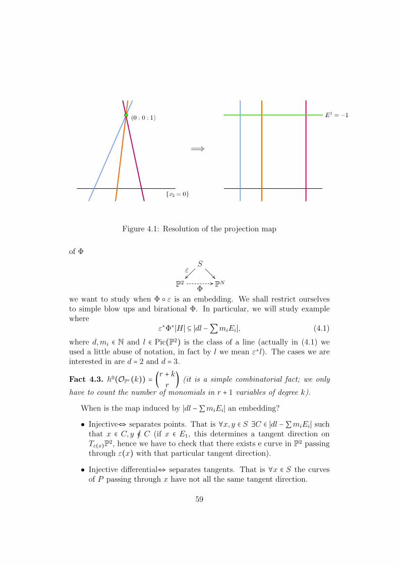
Figure 4.1: Resolution of the projection map
of Φ
S
P2 PN
............................................................................
ε ................................................................ ............
........................................................................ ............
Φ
we want to study when Φ ε is an embedding. We shall restrict ourselvesto simple blow ups and birational Φ. In particular, we will study examplewhere
ε∗Φ∗∣H ∣ ⊆ ∣dl −∑miEi∣, (4.1)
where d,mi ∈ N and l ∈ Pic(P2) is the class of a line (actually in (4.1) weused a little abuse of notation, in fact by l we mean ε∗l). The cases we areinterested in are d = 2 and d = 3.
Fact 4.3. h0(OPr(k)) = (r + kr
) (it is a simple combinatorial fact; we only
have to count the number of monomials in r + 1 variables of degree k).
When is the map induced by ∣dl −∑miEi∣ an embedding?
• Injective⇔ separates points. That is ∀x, y ∈ S ∃C ∈ ∣dl −∑miEi∣ suchthat x ∈ C, y /∈ C (if x ∈ E1, this determines a tangent direction onTε(x)P2, hence we have to check that there exists e curve in P2 passingthrough ε(x) with that particular tangent direction).
• Injective differential⇔ separates tangents. That is ∀x ∈ S the curvesof P passing through x have not all the same tangent direction.
59

Remark 4.4. Let S ⊂ PN smooth surface and N > 5. Then ∃ a projectionπ ∶ PN PN−1 such that π∣S ∶ S → π(S) is biregular.
Proof. When the projection map with center p ∈ PN does not work? If eitherp ∈ S (in this case the restriction π∣S would not be a morphism), or a linethrough p contains two points of S (in this case π∣S would not be injective),or a line through p is tangent to S (in this case π∣S would not separatestangents). Hence we can prove that the set of points that do not work isthe image of a variety X of dimension 5. In order to prove this, let usconsider the Zariski closure of the set (x, y, t) ∈ S × S × PN ∶ x ≠ y, t ∈ xy;basically, this subvariety of S × S × PN is the locus of the triples (x, y, t),where either t lies on the line passing through x and y when these are twodistinct points, or t belongs the tangent plane at x if x = y. This varietysurjects on S × S with a general fiber isomorphic to P1, hence its dimensionis (dimS × S) + dimP1 = 4 + 1 = 5.
Remark 4.4 gives the following result.
Proposition 4.5. Every projective surface is isomorphic, via generic pro-jection, to a smooth surface in P5.
4.1.1 Linear systems of conics
Since the number of conics in 2 variables is 6, the linear system P = ∣2l∣induces a map Φ ∶ P2 → P5 which is an embedding. The image of Φ is theVeronese surface V .
Remark 4.6. V contains no lines of P5.
Proof. Let C ⊂ V , then
degOC(H) = Φ−1(C) ⋅Φ∗H= Φ−1(C) ⋅ 2l = 2 deg Φ−1(C),
that is an even number. For a line this number is 1, so C cannot be a line.
On the other hand, let us consider l ⊂ P2 a line. 2l ⋅l = 2, hence Φ(l)⋅H = 2.This means that the lines of P2 are mapped onto conics in V .
Proposition 4.7. Let p ∈ P5 be a generic point. Then projecting away for pπp ∶ P5 P4 induces an isomorphism of V onto its image V ′ ⊂ P4.
We mention the following important characterization of the Veronese sur-face, which unfortunately we have no time to prove.
60

Theorem 4.8. ∀S ⊂ P5 non degenerate1, if ∃p ∈ P5 such that πp∣S is anembedding, then, up to a coordinate change, S is the Veronese surface.
Proof of Proposition 4.7. The lines of P2 are parametrized by (P2)∨ (the dualspace of P2). Each line l in P2 determines a plane containing the conic Φ(l).This defines a P2-bundle over (P2)∨ Y 4 ⊂ (P2)∨ × P5. The secant variety is
X5 ⊂ S × S × PN ∶= (p, q, t) ∶ t ∈ pq and p ≠ q;
in our case N = 5, S = V ⊂ P5. Let p, q ∈ S, then Φ−1(p)Φ−1(q) is a line in P2;this line is mapped into a conic C ⊂ P5, and pq is contained into the planecontaining C. Hence the image of X → S × S is contained in the image ofY → P5. Any six point p out of the image of Y will then do the job.
What if we project once more?
V ⊂ P5
smooth V ′ ⊂ P4
singular Steiner ⊂ P3
...........................................................................
general projection
...........................................................................
general projection
If we project P5 P4 away from p ∈ V the restriction π∣V is no longerdefined on the whole V . Resolving the map we get
P2 P4
F1
......................................................................... ............
..................
........................................
..........................................................
and the composition, induced by the linear system ∣2l −E∣, embeds F1 in P4.
f = l −EB = E
1X ⊂ PN is said to be non degenerate if /∃ PN−1⊂ PN a linear subspace X ⊂ PN−1.
61

In the description of Pic(F1), the system ∣2l −E∣ is given by ∣2f + b∣ = ∣h+ f ∣.Where is a fiber mapped?
f ⋅H = f ⋅ (2f + b) = 1,
hence each fiber is mapped into a line of P4. And where is B mapped?
b ⋅H = b ⋅ (2f + b) = 2 ⋅ 1 − 1 = 1,
hence B too is mapped into a line. Moreover, we can compute the degree ofthese surfaces.
degV = (2l)2 = 4;
degV ′ = (2l)2 = 4;
degF1 = (2f + b)2 = 4bf + b2 = 4 − 1 = 3.
With a little abuse of notation we wrote degF1; in fact, this computationwould be meaningless for the abstract Hirzebruch surface F1, it is possibleonly because in this case F1 is embedded into the projective space P4.
Exercise 4.9. Projecting a smooth surface S ⊂ PN away form a generalpoint, if the map we get is birational, then the degree of the image is thesame of the degree of the original surface. If the center of the projectionlies on the surface, still assuming the map to be birational, the degree of theimage decreases by one.
Projecting twice from points internal to the Veronese surface we get thesituation represented in the following:
P2 V4 ⊂ P5
F1 S3 ⊂ P4
furtherblow up
Q2 ⊂ P3
............................................................................................................................................................................................................................................................................................................... ............................
∣2l∣
.......
.......
.......
.......
.......
.......
.......
.......
.......
.......
.......
.......
.......
.......
.......
...............
............
...................................................................................................................................................................................................................................................................................................................... ............∣2l −E∣
.................................................................................................................................................................................................................................................................................. ................................................................................................................................................................................................................................................................................................... .................∣2l −E1 −E2∣
.....................................................................................
projection
.....................................................................................
projection..............................................................................................................
where, for a fixed p ∈ P2 (and, with a slight abuse of notation, p ∈ V4 is theimage of p), E is the exceptional divisor of the blow up F1 → P2 in p; themap V4 S3 is the projection with center p; p2 ∈ F1 (and, as before, p2 ∈ S3
62

will denote its image as well); E2 is the exceptional divisor of the blow up ofF1 in p2 and E1 the pull back of E; finally, S3 Q2 is the projection withcenter p2.
Let us begin from the top of the diagram and let us study the mapP2 V4 ⊂ P5. We denote the coordinates on P2 by (x0 ∶ x1 ∶ x2) and those onP5 by (y0 ∶ ⋅ ⋅ ⋅ ∶ y5). Let q0, . . . , q5 be a base for C[x0, x1, x2]2 (its dimensionis 6 by Fact 4.3).
The linear system ∣2l∣ induces a ring morphism
ϕ ∶ C[yi] Ð→ C[xj]yi z→ qi
more preciselyϕd ∶ C[yi]d Ð→ C[xj]2d.
What is the kernel of this map?
kerϕ = polynomials in yi variables whose pull back vanishes in P2= polymomials in yi variables that vanishes on V4= ideal that defines V4 in P5
It is immediate to see that kerϕ0 = 0 because ϕ0 = IdC is an isomorphismby definition (regardless the linear system we are considering). Moreover,since qi is a basis and V4 is non degenerate, kerϕ1 = 0.
Let us study kerϕ2. By 4.3, C[yi]2 ≅ C21 and C[xj]4 ≅ C15, hence
ϕ2 ∶ C21 → C15
and dim kerϕ2 ≥ 6. Let us choose the the qi in the simplest possible way.
q0 = x20 q1 = x0x1 q2 = x0x2
q3 = x21 q4 = x1x2 q5 = x2
2
∀(x0, x1, x2) ∈ C3 ∖ 0 the matrix
⎛⎜⎝
x20 x0x1 x0x2
x0x1 x21 x1x2
x0x2 x1x2 x22
⎞⎟⎠
has rank 1, hence ∀(y0 ∶ ⋅ ⋅ ⋅ ∶ y5) ∈ V4,
rk⎛⎜⎝
y0 y1 y2
y1 y3 y4
y2 y4 y5
⎞⎟⎠= 1;
63

this means that each 2×2-minor of that matrix is equal to zero on V4. Hencewe get six quadrics
y0y3 − y21, y0y4 − y1y2, y1y4 − y2y3, y0y5 − y2
2, y1y5 − y2y4, y3y5 − y24 (4.2)
that vanishes in V4.
Exercise 4.10. What we have seen so far proves that
V4 ⊂ V⎛⎜⎝
rk⎛⎜⎝
y0 y1 y2
y1 y3 y4
y2 y4 y5
⎞⎟⎠= 1
⎞⎟⎠,
Show that V4 is exactly the zero locus of the quadrics in (4.2).
Now let us study S3, the surface we obtain projecting V4 out of a pointp ∈ V4. By Exercise 4.9, S3 will have degree 3. The linear system ∣2l − E∣is the system of the conics passing trough the fixed point p. Let us denotethe coordinates in P4 by (z0 ∶ ⋅ ⋅ ⋅ ∶ z4), and fix Q0, . . . ,Q4 a basis for the setf ∈ C[x0, x1, x2]2 ∶ f(p) = 0. We have a ring morphism
ψ ∶ C[zi] Ð→ C[xj]zi z→ Qi
,
more preciselyψd ∶ C[zi]d Ð→ C[xj]2d.
Let us study the kernel of this map. As before, kerψ0 = kerψ1 = 0.
ψ2 ∶ C[zi]2 Ð→ C[xj]4,
and C[zi]2 ≅ C[xj]4 ≅ C15. Anyway ψ2 is not surjective, since all Qi vanishin p. Hence every quadric in zi will be mapped in a linear combination ofQiQj, that vanish in p twice. Therefore
Imψ2 ⊂ f ∈ C[xj]4 ∶ f vanishes at least twice in p.
How many conditions these assumptions determine?
Example 4.11. Let us suppose p = (1 ∶ 0 ∶ 0) and let
f4 = ax40 + bx3
0x1 + cx30x2 + x2
0A2(x1, x2) + x0B3(x1, x2) +C4(x1, x2)
be a generic quartic. Then
• f4(p) = 0⇔ a = 0;
64
• f4 singular in p⇔ b = c = 0.
• f vanishes in pÔ⇒ one linear condition on the coefficients of f ;
• f singular in pÔ⇒ two linear condition on the coefficients of f .
Hence dim Imψ2 ≤ 12 ⇒ dim kerψ2 ≥ 3. Therefore ∃Q0,Q1,Q2 ∈ C[zi]2
independent such thatS3 ⊂ V (Qi).
Remark 4.12. The quadrics Qi are irreducible; indeed, suppose that Qi =Π1 ∪Π2, then, since S is irreducible, either S = S ∩Π1 or S = S ∩Π2. HenceS ⊂ Πi is degenerate.
Q0 ∩Q1 =∶ Σ is a surface of degree
#Σ ∩H1 ∩H2´¹¹¹¹¹¹¹¹¹¹¹¸¹¹¹¹¹¹¹¹¹¹¹¹
P2
= 2 ⋅ 2 = 4.
S is a surface of degree #S ∩H1 ∩H2 = 3. Hence, defining Π ∶= Σ ∖ S,
#Π ∩H1 ∩H2 = 4 − 3 = 1,
thus Π is a plane. This means that the two quadrics Q0 and Q1 cut thesurface S and a plane in P4, the third quartic will get rid of this extra plane.
Π = l0 = l1 = 0 with li ∈ C[zj]1. Q0 and Q1 vanishes on Π⇔ Qi ∈ (l0, l1)(the ideal generated by l0 and l1). Hence
Q0 = l0A1 − l1A0, Q1 = l0B1 − l1B0 with Ai,Bj ∈ C[zj]1.
We shall rewrite the last equations as
Q0 = det(l0 A0
l1 A1) Q1 = det(l0 B0
l1 B1) .
Let us define
M = (l0 A0 B0
l1 A1 B1)
and Z = rkM = 1. Let P ∈ Σ. Let us suppose that l0(P ) ≠ 0, then in P
A1 =A0l1l0
, B1 =B0l1l0
;
A0B1 −A1B0 =A0B0l1l0
− A0B0l1l0
= 0,
65

hence P ∈ Z. Analogously we prove that l1(P ) ≠ 0 ⇒ P ∈ Z. Hence P ∈Σ ∖ Π ⇒ P ∈ Z. This means that S ⊂ Z and therefore A0B1 − A1B0 is inkerψ2. One could indeed prove that the 2× 2 minors of M generate kerψ byproving S = Z.
Let C ∶= S ∩Π; it is defined by l0 = l1 = A0B1 −A1B0, hence it is a conicin Π ≅ P2. Suppose to have a plane conic in S that is C2 ⊂ Π ≅ P2 such thatC2 ⊂ S. Let Σ ∶= S ∪Π; we want to compute the dimension of the space Wof the quadrics in C[zj]2 vanishing on Σ. Clearly W ⊂ span(Q0,Q1,Q2) ⊂C[zj]2.
Choose a point P ∈ Π∖C, hence P /∈ S, let
W ∶= f ∈ C[zj]2 ∶ f vanishes onS ∪ P
W ⊂ W ⊂ span(Q0,Q1,Q2) and since P /∈S dimW = 3 − 1 = 2.If Q ∈W , then Q ∩Π is a conic that con-tains C and P . Contradiction!Hence Q∩Π = Π, thus W =W , so dimW =2.
So we have proved the following proposition.
Proposition 4.13. The cubic ruled surface S ⊂ P4 is contained in a 2−dimensionallinear system of quadrics in P4, of which it is the intersection. For every pen-cil of quadrics λQ1+µQ2 containing S, Q1∩Q2 = S∪P , where P is a planeand S∩P a conic. Conversely, for every conic on S lying in a plane P , S∪Pis the intersection of two quadrics.
If we project once more, we get the bottom part of the diagram seenabove:
blow up↠ Q2 ⊂ P3.
Fact 4.14. If p2 /∈ B Q2 is smooth and ≅ P1 × P1.If p2 ∈ B, then B is contracted into a singular point of Q2.
4.1.2 Linear system of cubics
Let p1, . . . , pr ∈ P2 in general position (that is, that no triple of pis lies on aline, and none 6−tuples of pis lies on a conic). Let d = 9 − r and Sd the blowup of P2 in p1, . . . , pr with exceptional curves E1, . . . ,Er.
Theorem 4.15. If r ≤ 6 (that is d ≥ 3)∣ −KSd∣ = ∣3l −∑Ei∣ is very ample;
this means that such linear system embeds Sd in P10−r−1 = Pd.
66

Proof. Exercise. Hint: first study r = 6.
Fact 4.16. A surface S with ∣ −KS ∣ very ample is said to be a Del Pezzosurface. It is possible to prove that the only del Pezzo surfaces are Sd ⊂ Pdwith 3 ≤ d ≤ 9 and P1 × P1 ⊂ P8.
Let then study Sd Pd; first, let us compute the degree of such surface
degSd = #Sd ∩H1 ∩H2 = (3l −∑Ei)2
= 9l2 +r
∑i=1
E2i − 6∑ lEi − 2∑
i≠jEiEj
= 9 − r = d.
Hence del Pezzo surface of degree d is embedded in Pd.Let us study S3 ⊂ P3. As before, we have ring morphisms
ψd ∶ C[yi]d Ð→ C[xj]3d.
kerψ0 = kerψ1 = 0. Let us study the map
ψ2 ∶ C[y0, . . . , y3]2 Ð→ C[x0, x1, x2]6
C[yi]2 ≅ C10 and C[xj]6 ≅ C28, but we are interested only in those sexticspassing trough p1, . . . , p6 and singular in such points, hence we have 6×3 = 18linear condition. Thus the map
ψ2 ∶ C10 Ð→ C10 (4.3)
might be injective. The map ψ3 is
ψ3 ∶ C20 → C55−36 = C19, (4.4)
since the triple nonic passing trough p1, . . . , p6 determines 6 × 6 = 36 condi-tions. Hence dim kerψ3 ≥ 1.
It is possible to prove that the ideal of S3 is principal and generatedby a cubic; in particular dim kerψ2 = 0 and dim kerψ3 = 1 as the abovecomputation suggested.
Let us study now S4 ⊂ P4; for this surface we need at least two equations.Indeed
ψ2 ∶ C15 Ð→ C28−15 ≅ C13, (4.5)
since we have 3 linear conditions for each of the 5 points pi. Actually S4 is acomplete intersection surface of two quadrics in P4.
67

In fact, the computations in (4.3), (4.4) and (4.5) are a bit sloppy becausewe never checked that the conditions imposed by the points are independent.In particular, the target spaces could have dimension bigger than the onewe wrote. This is not the case. Let us prove, for example, that in (4.5)the target space actually is C13, that is we want to prove that h0(OS4(6l −2∑5
i Ei)) = 13 (∣6l − 2∑5i Ei∣ represents the linear system of sextics passing
with multiplicity two trough our five points). What we have proved so far isthat h0(OS4(6l − 2∑5
i Ei)) ≥ 13.Let H ⊂ P4 be an hyperplane. If H is generic, H ∩S4 ≅ C ⊂ P2 is a smooth
cubic passing trough p1, . . . , p5, hence an elliptic (hence of genus 1) curve.OS4(6l − 2∑5
i Ei) = OS4(2H), hence
0Ð→ OS4(2H −H)Ð→ OS4(2H)Ð→ OC(2H)Ð→ 0,
thus
h0(OS4(2H)) ≤ h0(OS4(H)) + h0(OC(2H))= h0(OS4(3l −∑Ei)) + h0(OC(2H))≤ 5 + χ(OC(2H))= 5 + deg(OC(2H)) = 5 + 2H ⋅C = 5 + 2 degS4 = 13.
Fact 4.17. Del Pezzo surfaces of degree 3 and 4 are complete intersections;
• S3 Ð→ one cubic equation in P3;
• S4 Ð→ two quadric equations in P4.
S5, . . . , S9 are not complete intersection; actually they need more than d − 2equations.
Let us study S3, in particular we want to see whether S3 contains somelines. As we have seen above, we have
Ei ∈ S3 P3
pi ∈ P2
......................................................................................................................................................................................................................................................................................................................................... ............................
∣3l −∑Ei∣ = ∣ −KS ∣...............................................................................................................................................................................
with p1, . . . , p6 points in general position. Let C ⊂ S3 be a line in P3. ThenC ≅ P1, and C ⋅ (3l −∑Ei) = 1 ⇔ KS ⋅C = −1, hence, by the genus formula,C2 = −1. Thus a line in S3 is an exceptional curve.
68

We know six of them, E1, . . . ,E6. Let us define ∀i < j
lij ∈ ∣l −Ei −Ej ∣;
these 15 curves are the strict transforms of the lines in P2 passing throughpi and pj. Moreover
(3l −6
∑k=1
Ek)(l −Ei −Ej) = 3l2 − 1 − 1 = 1,
hence each lij is a line. Let us define
qi ∈ ∣2l −6
∑k=1
Ek +Ei∣;
this is the strict transform of the conic in P2 passing through every pj exceptfor pi. Then each one of the six qi is such that
q2i = (2l −∑Ek +Ei)2 = 4l2 − 6 − 1 + 2 = −1.
Therefore what we have proved so far is that S3 contains at least 6+15+6 = 27lines of P3. We want to prove that no other line is contained in S3.
Firs of all, we shall remark that if we take two lines, they either haveintersection 0 (if they are disjoint) or 1 (if they intersect). One can easilycheck that the lines, among these 27, intersecting E1, are
l12 l13 l14 l15 l16
q2 q3 q4 q5 q6
Exercise 4.18. Verify that each of the above 27 lines intersects exactly 10of the other 26.
By 2.7, Pic(S) = Zl ⊕ ZE1 ⊕ ⋅ ⋅ ⋅ ⊕ ZE6 ≅ Z7, hence each C ∈ Pic(S) shallbe written in the following way:
C ≡ al −6
∑i=1
miEi.
Let us suppose that C is a line and C ≠ Ei, hence either C ⋅Ei = 0 or C ⋅Ei = 1.But C ⋅Ei =mi, hence mi ∈ 0,1. Furthermore, we know that C2 = −1, then
−1 = C2 = a2 −∑m2i ≥ a2 − 6,
hence a2 ≤ 5⇒ a ∈ 0,1,2 (a ≥ 0 otherwise C would not be effective). Hence
a = 0⇒ ∑m2i = 1⇒ C = Ei
a = 1⇒ ∑m2i = 2⇒ C = lij
a = 2⇒ ∑m2i = 5⇒ C = qi
69

Theorem 4.19. Let S be a smooth cubic in P3, then S is the blow up of P2
in 6 points in general position embedded by ∣3l −∑Ei∣.Proof. First of all, we study the Klein quadric; this is a set that parametrizesthe lines in P3 and has a natural structure of variety.
Let L ⊂ P3 be a line, and a, b ∈ L; then
a = (a0 ∶ a1 ∶ a2 ∶ a3)b = (b0 ∶ b1 ∶ b2 ∶ b3).
Let us define the map
⎛⎜⎜⎜⎝
a0 b0
a1 b1
a2 b2
a3 b3
⎞⎟⎟⎟⎠z→ (a0b1−b0a1 ∶ a0b2−a2b0 ∶ a0b3−a3b0 ∶ a1b2−a2b1 ∶ a1b3−a3b1 ∶ a2b3−a3b2)
This function, seen as a map lines in P3 → P5 is well defined, since ifwe change the two points and/or their homogeneous coordinates withoutchanging the line, it changes the matrix on the left, but the values at theright change only by a multiplicative constant. This map is not surjective:indeed
lines in P3 ∼Ð→ G ∶= y0y5 − y1y4 + y2y3 = 0 ⊂ P5.
Fact 4.20. The map lines in P3→ G is bijective.
One can easily prove that two different lines are mapped to two differentpoints of G, which is called the Klein quadric and therefore gives a goodparameter space for the set of lines in P3. Computing the derivative, onecan easily check that G is a smooth variety of dimension 4. Let us considerP = ∣OP3(3H)∣ (that is the linear system of the cubics in P3) and the setI ∶= (L,S) ∶ L ⊂ S ⊂ G × P .
I ∶= (L,S) ∶ L ⊂ S
G P
........................................................................................................
π1............................................................................................ ........
....
π2
Let us denote by (x ∶ y ∶ z ∶ t) the coordinates in P3. Let L ∈ G; up to a changeof coordinates, we shall suppose that L = z = t = 0, thus (L,S) ∈ π−1
1 (L)⇔S = f3 = 0,where f3 does not contain the monomials x3, x2y, xy2, y3 ≅ PdimP−4.Therefore, I is a smooth variety of (complex) dimension
dimI = dimG + dimP − 4 = 4 + dimP − 4,
that is dimI = dimP . Now let us consider π2: this is a map among twocomplex varieties of the same dimension. Then:
70
• either π2 has degree strictly positive and π2 is onto;
• or π2 has degree zero: in this case ∀p ∈ π2(I), p is not a regular valueand π−1
2 (p) is not a finite set.
We know that S3, the del Pezzo surface of degree 3, is a cubic and containsexactly 27 lines. This means that S3 ∈ π2(I) and π−1
2 (S3) is finite. Hence π2
cannot have degree 0 and it is onto. This means that each cubic contains aline of P3: ∀S ∈ ∣OP3(3)∣ ∃L ⊂ S with L line of P3.
Let S be a smooth cubic in P3, L a line contained in S. We want to findall the lines in S intersecting L. Since two lines intersecting in a point arecontained in the same plane, let us study the pencil of planes L ⊂ H. Up toa change of coordinates, we may suppose that L = z = t = 0, hence we get anatural explicit parametrization of the pencil of planes by associating to eachpoint (a ∶ b) ∈ P1 the plane az + bt = 0. It is easy to see that H ∩S = L∪C,where C is a conic; if H is a general plane, C will be smooth, otherwise, Ccould be the union of two lines (possibly a double line). We want to studyin which case the conic we get is non smooth. Let us write the equation ofS in the following way:
Ax2 + 2Bxy +Cy2 + 2Dx + 2Ey + F, (4.6)
where A,B,C,D,E,F ∈ C[z, t] with degA = degB = degC = 1, degD =degE = 2 and degF = 3. Written as (4.6), the equation looks like theequation of a conic, whose rank depends on the matrix
M ∶=⎛⎜⎝
A B DB C ED E F
⎞⎟⎠
;
detM ∈ C[z, t]5, hence its zero locus is the union of H1, . . . ,H5, 5 planesthrough L. Since S is smooth, it is possible to prove that
• H1, . . . ,H5 are distinct (that is detM is square free);
• ∀Hi, Hi∩S = L∪Li∪L′i are three distinct lines. Moreover, for each planeH in the pencil different from these 5, since the rank of M becomes 3,the intersection H ∩ S is the union of a line and a smooth conic.
Hence we have found 11 lines contained in S, and we know that every otherline in S would be disjoint form L. If 3 distinct lines in S meet at a pointp ∈ S, then, since S is smooth, they lie in the tangent plane to S at p, and sothey are coplanar. Now consider L1 and L2, they are not coplanar (because
71

H1 ≠H2), so L∩L1 and L∩L2 are distinct. It easily follows that (again sincethey are not coplanar) L1 ∩L2 = ∅. Let us define then two birational maps
Φ ∶ L1 ×L2 ≅ P1 × P1 S
Ψ ∶ S L1 ×L2 ≅ P1 × P1
• For p, p′ general point in L1 and L2 respectively, then Φ(p, p′) = p′′,where p′′ is the only intersection different from p and p′ of pp′ and S.This function is not defined if pp′ ⊂ S;
• ∀s ∈ S ∖ (L1 ∪ L2) let Π1 be the plane passing through s and L1, letΠ2 be the plane passing through s and L2 and L′ ∶= Π1 ∩Π2, then wedefine Ψ(s) = (L′ ∩L1, L′ ∩L2).
It is easy to see that Φ is the inverse of Ψ and vice versa. Hence S is rational.Moreover, Ψ can be extended to a morphism: if s ∈ L1 we take Π1 ∶= TsS, ifs ∈ L2 we take Π2 ∶= TsS. Therefore we have a map
Ψ ∶ S → P1 × P1,
that is a birational morphism, and so a sequence of blow ups, as many as arethe curves contracted by Ψ. Let us count these curves.
Let s1, s2 ∈ S ∖ (L1 ∪ L2) and suppose Ψ(s1) = Ψ(s2) = (p, p′), thens1, s2 ∈ pp′ ⇒ #pp′ ∩ S ≥ 4 > 3 ⇒ pp′ ⊂ S. This means that the curvescontracted by Ψ are exactly the lines that intersect both L1 and L2. Weproceed to calculate the number of these lines. We know that the linesmeeting L fall into 5 pair (Li, L′i) with 1 ≤ i ≤ 5. such that Li, L′i and L lie ina plane Hi. Hi meets L2 in one point, which lies on Li or L′i (but not both,for else, Li, L′i and L2 would be coplanar). Thus one line in each pair meetsL2 as well, and so Ψ contracts 5 lines.
S
SIV
SIII
SII
SI
P1 × P1 F1
P2
..........................................................
..........................................................
..........................................................
..........................................................
..........................................................
......................................... ............
......................................... ............
Hence (see the diagram on theleft) S is a blow up of P2 in sixpoints. Moreover, it is not difficultto prove that H = 3l∖(E1∪⋅ ⋅ ⋅∪E6),that is that S is embedded by thesystem of cubics through the sixpoints; in other words, S is a delPezzo surface S3.
72

Chapter 5
Castelnuovo’s Theorem and itsapplications
5.1 Castelnuovo’s Theorem
At the end of 19th century, it was a well known fact that if C is a projectivesmooth curve such that h0(Ω1
C) = 0, then C ≅ P1. What happens in dimension2? In the previous chapter we have seen that for a surface S q(S) ∶= h0(Ω1
S)and pg(S) ∶= h0(Ω2
S) are birational invariants, moreover q(P2) = pg(P2) = 0,hence it is immediate to conclude that if S is a smooth projective rationalsurface, then q(S) = pg(S) = 0. Does the opposite implication hold, as in thecase of the curves?
Conjecture 5.1 (Max Noether’s conjecture). If S is a smooth projectivesurface, with q = pg = 0, then S is rational.
Enriques built a counterexample to Noether’s conjecture; in particular,he defined a non rational surface S with q = pg = 0 and P2 = 1.
The construction of Enriques gave the motivation to Castelnuovo to proveits important criterion.
Theorem 5.2 (Castelnuovo’s rationality Criterion). Let S be a projectivesurface with q = P2 = 0, then S is rational.
Let us recall that
pg ∶= h0(OS(KS)) P2 ∶= h0(OS(2KS)).
Remark 5.3. If pg ≠ 0, then P2 ≠ 0; indeed, if σ ∈ H0(OS(KS)), thenσ2 ∈ H0(OS(2KS)). The opposite implication does not hold by, e.g., theabove mentioned Enriques’ construction.
73

In order to prove Theorem 5.2, we need the following proposition.
Proposition 5.4. Let S be a minimal projective surface with q = P2 = 0,then ∃C ⊂ S smooth curve such that C ≅ P1 and C2 ≥ 0.
We do not give the full proof of Proposition 5.4, but only a short sketch,to give an idea on how the hypotheses are used.
Proof of Theorem 5.2. We shall assume, without loss of generality that S isminimal, then, by Proposition 5.4, there exists C ⊂ S smooth curve such thatC ≅ P1 and C2 ≥ 0. Let us consider the exact sequence
0Ð→ OS Ð→ OS(C)Ð→ OC(C)Ð→ 0.
OC(C) ≅ OP1(C2), hence we get the exact sequence
0Ð→H0(OS)Ð→H0(OS(C))Ð→H0(OP1(C2))Ð→H1(OS)Ð→ . . . ,
but H1(OS) =H0(Ω1S) = 0 by q = 0, hence the sequence becomes
0Ð→H0(OS)Ð→H0(OS(C))Ð→H0(OP1(C2))Ð→ 0;
moreover H0(OS) ≅ C (because S is compact) and H0(OP1(C2)) ≅ CC2+1.Hence h0(OS(C)) = C2+2 ≥ 2 (that is the curve C is not rigid) and dim ∣C ∣ =h0(OS(C))−1 ≥ 1. This implies that there exists an effective divisor differentfrom C and linearly equivalent to it. Moreover, since C is irreducible, ∣C ∣has no fixed part.
Taking a pencil D contained in ∣C ∣ without fixed part, it defines a mapon P1
S
S P1
............................................................................
................................................................ ............
ϕ
......................................................................... ............
Resolving the map, we get a surjective morphism ϕ with basis P1 and a fiberisomorphic to C ≅ P1 (the strict transform of C). Hence by Theorem 3.5 Sis ruled on P1 and we get the thesis.
Sketch of the proof of Proposition 5.4. By Serre duality
0 = h0(2K) = h2(−K)
hence 1 +K2 = χ(−K) = h0(−K) − h1(−K) + h2(−K) ≤ h0(−K). In the proofone distinguishes three cases: K2 < 0, K2 = 0, K2 > 0. We consider only thecase K2 = 0. For K2 = 0, we have h0(−K) ≥ 1, hence −K ≥ 0. Let us fixH ∈ Pic(S) very ample, and let us study ∣H + nK ∣: since −K ≥ 0, ∃n suchthat ∣H + nK ∣ ≠ ∅ and ∣H + (n + 1)K ∣ = ∅: fix D ∈ ∣H + nK ∣. D is effectiveand the following properties hold:
74
• ∣K +D∣ = ∅;
• K ⋅ D < 0 indeed K ⋅ D = K ⋅ H + nK2 = −H ⋅ (−K) < 0, where lastinequality holds because H is ample and −K is effective.
D = ∑niCi with Ci is curve and ni > 0 ∀i. Since ∀i D −Ci ≥ 0, h0(K +Ci) ≤h0(K +D) = 0⇒ ∀i ∣K +Ci∣ = ∅. Moreover, ∃i such that K ⋅Ci < 0, otherwisethe second property seen above would not hold. Hence there exists C < Dirreducible such that ∣K + C ∣ = ∅ and K ⋅ C < 0. Since C is irreducible, wecan exploit 1.104 to compute the arithmetical genus
0 ≤ pa(C) = 1 + K ⋅C +C2
2⇒K ⋅C +C2 ≥ −2
Since K ⋅C < 0, C2 ≥ −1.If C2 = −1, then
0 ≤ 1 + KC − 1
2< 1⇒KC = −1, pa(C) = 0⇒ C ≅ P1
by Exercise 2.29. But this gives a contradiction, since S by hypothesis isminimal. Thus C2 ≥ 0.
Now we prove that C ≅ P1. Since ∣K +C ∣ = ∅
0 = h0(K +C) ≥ χ(K +C) (1.10)= χ(O) + (K +C)(K +C −K)2
= (1 − q + pg) +KC +C2
2
by assumption q = 0 and by Remark 5.3 P2 = 0⇒ pg = 0, hence 1 − q + pg = 1,thus
0 ≥ 1 + KC +C2
2= pa(C)⇒ 0 ≥ pa(C),
thus we conclude that pa(C) = 0 and C ≅ P1.
Remark 5.5. Let f ∶ S′ ↠ S a surjective morphism among two surfaces; itinduces an injective pull-back map
f∗ ∶H0(Ω2S)H0(Ω2
S′),
and more generally injective maps
f∗ ∶H0(ΩiS)H0(Ωi
S′).
Thuspg(S′) ≥ pg(S), q(S′) ≥ q(S),
and analogously one can prove
P2(S′) ≥ P2(S), Pn(S′) ≥ Pn(S).
75

Definition 5.6. A variety X of dimension n is said to be unirational if thereexists a map from Pn to X that is dominant, that means that its image isdense.
Corollary 5.7. If S is an unirational surface, than it is rational.
Proof. Since pg(P2) = P2(P2) = 0, by Remark 5.5, pg(S) = P2(S) and byTheorem 5.2 S is rational.
The Corollary holds even for unirational varieties with n = 1, but doesnot hold for n ≥ 3.
Theorem 5.8. Let S be a minimal rational surface, then either S ≅ Fn withn ≠ 1 or S ≅ P2.
Proof. We fix a very ample divisor H. Let us define
A ∶= C smooth ,C ≅ P1,C2 ≥ 0 ≠ ∅.
Let m ∶= minC∈AC2 ≥ 0 and let us choose C ∈ A with C2 = m and H ⋅ Cminimal. In other words, for every smooth rational curve C1 with C2
1 = m,H ⋅C1 ≥ H ⋅C > 0 (the second inequality follows as usual since C is effectiveand H is ample).
1. We first prove that ∀D ∈ ∣C ∣ , D ≅ P1 smooth. Let D = ∑niCi ∈ ∣C ∣.
(K +D) ⋅C = (K +C) ⋅C = −2 < 0
by genus formula. Since C2 ≥ 0, it follows ∣K+D∣ = ∅ and then ∣K+Ci∣ =∅ ∀i. Thus 0 = h0(K + Ci) ≥ χ(K + Ci) = pa(Ci) ∀i, where the lastequality holds by the Riemann-Roch Theorem. Hence by Exercise 2.29∀i Ci ≅ P1 smooth. K ⋅ C ≤ −2 < 0 ⇒ ∃i such that K ⋅ Ci < 0 and, byminimality of S (arguing as in the proof of Proposition 5.4), C2
i ≥ 0.Thus Ci ∈ A.
C2 = C ⋅D = C ⋅Ci+C ⋅(D−Ci) = C2i +(D−Ci)⋅Ci+C(D−Ci) ≥ C2
i , (5.1)
where last inequality holds since D−Ci, C, Ci are effective, and both Cand Ci are irreducible with non negative selfintersection. By the min-imality of m, (5.1) implies that C2
i = m. Moreover, by the minimalityof H ⋅C,
Ci ⋅H ≥ C ⋅H =H ⋅D =H ⋅Ci +H(D −Ci);
since H ⋅ (effective divisor) > 0, D − Ci = 0, thus D = Ci and we aredone.
76

2. We deduce that h0(OS(C)) ≤ 3. Let us fix p ∈ S general enough (p /∈ C)and, for each element of H0(OS(C)) let us consider the first term ofits Taylor expansion in a neighbourhood of p; we get a map
eval ∶H0(OS(C))→ Op/m2 ≅ C[x, y]/(x, y)2 ≅ C3,
where x, y are coordinates defined in a neighbourhood of p; basically iff ∈H0(OS(C))
eval(f) = f(0) + ∂f∂x
(0)x + ∂f∂y
(0)y.
If h0(OS(C)) ≥ 4, then dim ker eval > 0, thus ∃f ∈ H0(OS(C)) singularin p ⇒ (f) ∈ ∣C ∣ is singular in p. But this contradicts the first step ofthe proof.
3. Finally we prove is that m ∈ 0,1. Let us consider the exact sequence
0Ð→ OS Ð→ OS(C)Ð→ OC(C)Ð→ 0;
since q = 0 = h1(OS), then 3 ≥ h0(OS(C)) = h0(OS) + h0(OC(C)) =1 +m + 1 =m + 2, thus 0 ≤m ≤ 1.
• m = 0⇒ h0(OS(C)) = 2; we have a morphism S → P1 (the numberof base points is bounded from above by C2 = 0, hence there are nobase points) whose fibers are P1 (since ∀D ∈ ∣C ∣, D ≅ P1); thereforeS is geometrically ruled so by Proposition 4.1 and Theorem 4.2S ≅ Fn with n ≠ 1.
• m = 1 ⇒ h0(OS(C))) = 3; we have a morphism S → P2 and it iseasy to prove that is a biregular morphism (one first prove that:the linear system has no fixed part, then that it has also no basepoints and finally construct an inverse of the map).
5.2 Complex tori
Let V be a complex vector space of finite dimension m; let Γ ⊂ V be a lattice,that is Γ ⊂ B is a subgroup respect to the sum, Γ ≅ Z2m and generates V asa real vector space. T = V /Γ is a compact variety (with a natural structureof group) said complex torus. If T is projective, T is said to be an abelianvariety.
77

The projection on the quotient π ∶ V → T is a covering map and
dπp ∶ TpV ≅ V → Tπ(p)T
is an isomorphism ∀p ∈ V and gives a canonical identification between Vand TqT ∀q ∈ T . Let ui be a coordinate of V ; then dui ∈ H0(Ω1
V ) anddui ∈ V ∗ ≅ Cm, and it defines a section dui ∈ H0(Ω1
T ) (by a slight abuse ofnotation we will also denote by dui the pull back π∗dui). This implies thath0(Ω1
T ) ≥m.Moreover, if ω ∈ H0(Ω1
T ) then π∗ω ∈ H0(Ω1V ); π∗ω = ∑ fidui where fi are
holomorphic and Γ−periodic functions, thus fi is constant ∀i.
Corollary 5.9. π∗ ∶H0(Ω1T )
∼Ð→H0(Ω1V ) = V ∗.
This implies that if dimT = 2, then q = 2.
Theorem 5.10. Let T1 ∶= V1/Γ1, T2 ∶= V2/Γ2 be two complex tori and u ∶T1 → T2 holomorphic. Then u = t a, where t is a translation and a a grouphomomorphism.
Proof. We exploit the properties of the universal covering: ∃! u ∶ V1 → V2
such that the diagram
V1 V2
T1 T2
.................................................................................................... ............u
................................................................................................................
π1
................................................................................................................
π2
.................................................................................................... ............u
commutes. It is immediate to prove that u is holomorphic because π1 andπ2 are local diffeomorphisms. ∀x ∈ T1, ∀γ ∈ Γ1 u(x + γ) − u(x) ∈ Γ2, that is adiscrete set. Hence for every fixed γ, u(x + γ) − u(x) is constant as functionof x ∈ V1. Hence ∂u/∂zj are Γ−periodic and therefore (by the maximumprinciple) constant functions. This means that u is affine, that is u(x) = Ax+band clearly AΓ1 ⊂ Γ2; the map x↦ Ax goes down to a group homomorphism,and Ax↦ Ax + b descends to a translation.
5.3 Albanese variety
We give the following Theorem, called universal property of Albanese variety,without proof.
Theorem 5.11. Let X be a smooth projective variety. Then ∃! A ∶= Alb(X)abelian variety and a morphism
α ∶X → Alb(X)
78

with connected fibers such that ∀f ∶X → T with T complex torus ∃! f ∶ A→ Tsuch that the diagram
X
A T
...........................................................................
α................................................................................................... ........
....
............................................................... ............
commutes. The abelian variety A = Alb(X) is called the Albanese varietyof X and α is called Albanese map. Moreover the morphism α induces anisomorphism
α∗ ∶H0(Ω1A)→H0(Ω1
X)
Let us see some consequences of Theorem 5.11.
1. If H0(Ω1X) = 0 (for example X = Pn, rational surfaces or with q = 0)
then each map X → T is constant.
2. ∀F ∶ X → Y morphism of smooth projective varieties, there exists aunique morphism Alb(F ) ∶ Alb(X)→ Alb(Y ) such that the diagram
X Y
Alb(X) Alb(Y )
....................................................................................................................................................................................................................................................................... ............F
...........................................................................
αX...........................................................................αY
........................................................................................................................................................................................................ ............Alb(F )
commutes.
3. α(X) is not contained in any sub-torus T ′ ⊂ Alb(X), indeed, consider-ing X → T ′ the uniqueness is contradicted. In particular, if H0(Ω1
X) ≠ 0α(X) is not reduced to a point, that is α is not constant. This impliesthat α is constant⇔ H0(Ω1
X) = 0, hence α is constant ⇔ q = 0.
4. If X is a curve, then α is the Abel-Jacobi map, Alb(X) is equal to theJacobian JX and
α ∶X → JX
is embedded as a smooth curve.
Proposition 5.12. Let S be a projective smooth surface, α ∶ S → Alb(S) theAlbanese map. Suppose that α(S) = C is a curve. Then C is a smooth curveof genus q.
The following lemma is given without proof.
79

Lemma 5.13. Let S be a smooth projective surface and C an irreduciblecurve; let η ∶ C → C the normalization of C (that is C is a smooth curve andthe map η is generically injective) then ∃S → C such that
S C
C
................................................................................................... ............
............................................................... ............
...........................................................................
commutes.
Proof of Proposition 5.12. We have a commutative diagram
S
C ⊂Alb(S)
C
Alb(C) = JC
........................................................................... ............
.............................................................................................................................
...........
α
........................................................................................................................ ............u
.................................................................................................................................... v
.......................................................................................................................................................................................................................... ............
.......................................................................................................................................................
where both u and v exist by the universal property. Moreover, by uniqueness,u = v−1. Hence α(S) = C ⊂ JC = Alb(C) = Alb(S), hence it is smooth ofgenus dimJC = dim Alb(S) = q.
Hence for all S projective we have three possibilities:
• q = 0;
• dimα(S) = 1 and α(S) = C JC smooth curve of genus q;
• dimα(S) = 2.
Lemma 5.14. If pg = 0 and q ≥ 1, then dimα(S) = 1.
Proof. Since q ≠ 0 dimα(S) ≠ 0. If dimα(S) = 2, let then p ∈ Alb(S) be asmooth point, then there exists Tpα(S) ⊂ Tp Alb(S); we shall remark that
p ∈ α(S) ⊂ Alb(S) = V /ΓTpα(S) ⊂ Tp Alb(S) ≅ V.
Let u1, u2 ∈ V independent directions in Tpα(S). Let
ω ∶= du1 ∧ du2 ∈H0(Ω2(Alb(S)))
that does not vanish identically on Tpα(S) ⊂ V . Then α∗ω ∈H0(Ω2(S)) doesnot identically vanish in α−1(p). Hence pg(S) ≠ 0: a contradiction.
80

Theorem 5.15. Let Φ ∶ S S′ be a birational map among two non ruledprojective surfaces. If S and S′ are minimal, then Φ is biregular.
Another way to state Theorem 5.15 is that non ruled surfaces have aunique minimal model.
Proof. The only thing to prove is that Φ is a morphism. Let us resolve Φ inthe way outlined in the following diagram:
S
S S′
...........................................
εn............................................
................
. . .............................................
................
ε1
.............................................................................................................................................. ............
f
........................................................................................................................................... ............
let n be the minimum number of blow ups necessary to resolve Φ. Arguingby contradiction, let us suppose that n > 1; let E be the exceptional curveof εn: E ≅ P1, E2 = −1 and K ⋅E = −1. f ∣E is not constant, since otherwiseε1 ⋅ ⋅ ⋅εn−1 would have resolved Φ as well. C = f(E) is an irreducible divisorin S′, hence E is the strict transform of C. Recall that f is also a compositionof blow ups. Then one of the following occurs:
• None of the blow ups composing f involves points of C;
• Some of those blow ups involves points of C.
In the first case f ∣E ∶ E → C is an isomorphism, C ≅ P1, C2 = E2 = −1 andKS ⋅E = KS′ ⋅C = −1, contradicting the minimality of S′. Hence the secondcase holds; then E is the strict transform of C and by the formulas of the blowups (see Exercise 2.10) we deduce that C2 > E2 andKS′ ⋅C <KS ⋅E = −1. Sincepa(C) ≥ 0, by the genus formula, C2 ≥ 0. Note that these two inequalitiesimply
(nK ′S) ⋅C ≤ −2n < 0 ∀n ≥ 1,
hence ∣nKS′ ∣ = ∅; indeed, if ∣nKS′ ∣ contains a divisor D, then D ⋅ C ≥ 0,since every curve with positive autointersection number intersects any effec-tive divisor nonnegatively. This means that Pn = 0 ∀n ≥ 1. We must nowdistinguish two cases:
• If q = 0, then, taking into account that P2 = 0, Castelnuovo’s Theoremimplies that S′ is rational, which is excluded by hypotheses.
• If q ≥ 1, pg = 0 Pn = 0 ∀n. Then by Theorem 5.11 and Proposition 5.12,there exists
α ∶ S′ → B ⊂ Alb(S′)
81
with B smooth curve of genus q and Alb(S′) abelian variety of dimen-sion q. By Lemma 3.11 every map from E to B is constant; consideringthe composition
Ef ∣EÐ→ C
α∣CÐ→ B
it follows that α∣C is constant. Therefore C is contained in a fiber ofα. By Lemma 3.7 C2 ≥ 0, then C2 = 0 and rC with r ≥ 1 is a fiber ofα. Moreover K ⋅C ≤ −2, thus the genus formula implies
0 ≤ pa(C) = 1 + C2 +K ⋅C
2≤ 0,
hence pa(C) = 0, C ≅ P1 and K ⋅ C = −2. Albanese map has a regularvalue, hence for p ∈ Reg(α) Fp = α∗p is a smooth fiber. Since it isconnected, it is irreducible. By the genus formula
0 ≤ pa(Fp) = 1 + K ⋅ F + F 2
2
(#)= 1 + K(rC) + (rC)2
2= 1 − r,
where equality (#) holds for Remark 3.4. Hence r ≤ 1, thus r = 1. TheNoether-Enriques Theorem implies that S′ is ruled over B, a contra-diction.
5.4 Surfaces with pg = 0 and q ≥ 1
Studying the Albanese map of these surfaces one can prove that they arequotients of the product of two curves by the action of a finite group. Wegive the precise statement of their classification without proof.
Theorem 5.16. S is a minimal projective surface with pg = 0 and q ≥ 1 ifand only if S = (B × F )/G where B,F are Riemann surfaces, G is a finitegroup, with
G Aut(B) G Aut(F ),
that acts over B × F in the natural way (that is g(b, f) = (gb, gf) for g ∈ G,(b, f) ∈ B × F ) and
• B/G is an elliptic curve;
• F /G ≅ P1;
• one of the following holds:
82

1. B is elliptic and G is a translation group;
2. F is elliptic and G acts freely on B × F .
This implies that q = 1 and K2 = 0.
83