This module deals with the important topic of how one evaluates an

estimated model, determines if it is sufficient, and evaluates the

support from data.

Notes: IP-056512; Support provided by the USGS Climate & Land

Use R&D and Ecosystems Programs. I would like to acknowledge

formal review of this material by Jesse Miller and Phil Hahn,

University of Wisconsin. Many helpful informal comments have

contributed to the final version of this presentation. The use of trade

names is for descriptive purposes only and does not imply endorsement

by the U.S. Government.

Last revised 17.01.31.

Source: https://www.usgs.gov/centers/wetland-and-aquatic-research-

center/science/quantitative-analysis-using-structural-equation

1

For unsaturated networks, we have two different, though related, issues

to consider, the first being a bit novel.

2

I don’t expect you to be able to read all this. For now I just want to

make the point that lavaan will give you a great deal of information if

you ask for it using “fit.measures=T” in the summary command.

3

Actually, lavaan calculates even more fit indices, which requires a

different command to obtain “fitMeasures(fit.object)?

Again, I don’t expect you to read all this. For now just know that

SEMers have been preoccupied with this topic since the early 1970s.

Note, in this module I will provide you with a practical approach to

evaluating models. There are many different approaches that can be

used and I fear it will be distracting to you if I cover a broad variety of

perspectives. So, I am, for now, ignoring many of the options, while

providing a sufficient set of test procedures for the basic task.

4

5

We should not expect typical data sets to be our definitive source of

conclusions for causal models. This seems like a radical idea, but the

current data set is not our total knowledge on a subject. Causal

modeling has to be built through knowledge accumulation.

6

A minimum requirement for network models under global estimation is

that no links of major importance are omitted. If they are we should not

believe the parameter estimates. DON’T use such models for

interpretation.

7

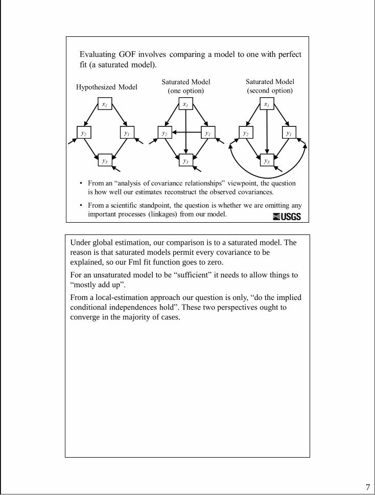
Under global estimation, our comparison is to a saturated model. The

reason is that saturated models permit every covariance to be

explained, so our Fml fit function goes to zero.

For an unsaturated model to be “sufficient” it needs to allow things to

“mostly add up”.

From a local-estimation approach our question is only, “do the implied

conditional independences hold”. These two perspectives ought to

converge in the majority of cases.

8

It was noted early on in modern SEM that the fit function follows a

chi-square distribution. We calculate our model “Chi-square statistic”

directly from the model discrepancy, summed over the samples.

Important here is the single-degree-of-freedom criterion, which is a

handly device in SEM.

9

This slide serves as a reminder that overall goodness of fit involves

reference to a saturated model and for the classic-type model we are

dealing with, such models have zero discrepancy.

Here, once again, is the generic example model from the module “Brief

Intro to Lavaan”. Again, three steps in lavaan:

(1) specify model using lavaan’s code,

(2) use the “sem” function to estimate the parameters (“fit”) for the

specified model, and

(3) extract information from the fitted object.

10

Here in blue is output in R. Now we understand that a chi-square of 17

with 2 df and a p-value less than 1 in 1000 indicates a large

discrepancy between data and model-implied covariances.

11

When we have a discrepant model, we need help sometimes in

knowing where to look for suggested changes. Lavaan like all sem

software can compute “modification indices”. These are uninformed

suggestions that should not be followed blindly.

In this case, we already know what the logical candidates for additional

paths are. If we have some experience with SEM and with this system,

we will have already thought about some of the reasons variables might

not be conditionally independent.

Of course we could just saturate our models at the outset, looking for

everything and then just prune paths. That is fine for exploratory

modeling, but not good practice for confirmatory modeling.

Here I show results for the two missing connections. Shown are both

correlations and directed relationships, both of which would yield

similar improvements in model fit, though mean very different things

scientifically.

We can ignore the epc, but the mi is an estimated reduction in model

chi-square we would presumably obtain by including that link.

12

13

Based on what we have seen and what we know about the variables, we

would be likely to add a directed path from x1 to y3. This is still not a

saturated model, so we will still get a test as to whether it is as good as

a saturated model.

For Model 2, we add the bit in red to complete the code.

14

Adding the link made a big different. Our results imply y1 and y2

cannot explain all effects of x1 on y3.

15

16

Formally, here is where we would rely on the single-degree-of-freedom

chi-square test. The observed drop of 17.715 greatly exceeds the

criterion of 3.84 for a classical, p-value based hypothesis test.

17

We can perform likelihood-ratio tests for a set of models using the

‘anova’ function with a lavaan object. Aside from giving AIC values

for models to compare, it also automates a chi-square comparison

between models.

18

OK, we have made sure we are not missing major links in our model.

Only now can we begin to address the question of whether we have

paths in the model that are not supported by the data.

19

Interest in AIC for model comparison has grown in biology. There are

lots of important points that could be made about this, but I will save

that for another time and place. What is most relevant, it to understand

that since classical SEM is a model-centered, likelihood-based

approach, AIC is a direct computation from the Model Fit Function.

A key reference for the use of AIC is

Burnham, K.P. and Anderson , D.R. 2002. Model Selection and

Multimodel Inference. 2nd Ed. Springer Verlag.

There is a Forum of viewpoints provided in Ecology recently that

discuss the merits of p-values and AIC.

http://www.esajournals.org/toc/ecol/95/3

20

At the moment, for moderate to small samples (250 samples or less),

the AICc seems like a good choice for model selection.

With the AICc, we adjust the AIC for the ratio of information/samples

to parameters in the model. This is a reasonable suggestion because it

takes information to estimate parameters and the ratio of information to

parameters is a handy way to discuss sample size recommendations,

though such things are truly not simple.

Anyway, the AICc has a more complex parsimony correction term than

does the AIC (which is just 2q), as shown in the slide.

21

Whether one is using the AIC, AICc, or BIC, the guidelines for simple

interpretations are the same.

22

Since the utility of AIC shines when comparing a set of models, here

we throw in a third model, which allows y1 and y2 to have correlated

errors.

For Model 3, we add the bit in red to specify an error correlation.

23

24

Jarrett Byrnes from Univ. Mass at Boston has developed a function for

computing AICc for lavaan models. It can be obtained from his website

at:

http://jarrettbyrnes.info/ubc_sem/lavaan_materials/lavaan.modavg.R

Using this function allows us to simply compute the AICc differences

for a candidate set.

The simplest way to evaluate a set of models is to rank them by AICc

values and look for the smallest value. For a difference between

models to be “important-ish”, the Delta-AICc should be greater then

2.0. If the difference is less than that, I might be inclined to choose the

model with the fewer paths, since in a situation the evidence suggests

that adding a path does not improve the model substantially.

25

There is a bit more that can be done beyond computing delta AICc.

Here I show output from the command given on the previous slide.

There are a few things here, including:

AICc

Delta_AICc

AICcWt

Other things presented in upper table include Cumulative weight and

the raw log likelihoods, neither of which are important for our

discussion here.

Reference for this material.

Anderson, D. (2008) Model Based Inference in the Life Sciences: A

Primer on Evidence. Springer Verlag. (p 89)

Here are the basic parameter results. Note you can count the 8

parameters here that are shown as K for Model 2 on the previous page.

We now can begin to interpret results. Generally not a good idea to

worry about interpretation before selecting a model that (1) contains all

important links and (2) is found to be the best choice amongst model

options.

Glancing at the p-values for the parameters provides us with another

diagnostic, much like the modification indices. WE SHOULD NOT

TRUST THE PARAMETER P-VALUES AS A SOLE SOURCE OF

INFORMATION. To elaborate, the overall model has a behavior that

we are evaluating. It is not uncommon for parameter p-values to be

greater than 0.05, but then when you remove the associated link from

the model, overall discrepancy goes up significantly. TO REPEAT,

PARAMETER P-VALUES ARE ONLY DIAGNOSTICS, NOT

DEFINITIVE SOURCES FOR DECISIONS.

26

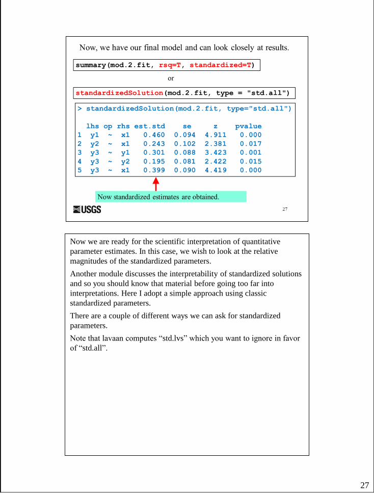
Now we are ready for the scientific interpretation of quantitative

parameter estimates. In this case, we wish to look at the relative

magnitudes of the standardized parameters.

Another module discusses the interpretability of standardized solutions

and so you should know that material before going too far into

interpretations. Here I adopt a simple approach using classic

standardized parameters.

There are a couple of different ways we can ask for standardized

parameters.

Note that lavaan computes “std.lvs” which you want to ignore in favor

of “std.all”.

27

Here is one of the many ways you might present your results, along

with various tables of total effects in the models or scenario findings.

You should also present model fit results.

A separate module will be developed soon for a more complete

discussion of results presentation. For now, consulting some of the

published papers for examples would be a good idea.

28

29

OK, after considering all this quantitative weighing of evidence in your

data set, I want to again emphasize you still have to consider many

things in decide what you believe about the system under investigation

from all your information sources. The next slide gives one example of

the latitude I suggest you give yourself.

30

Here is one of our examples where a “non-significant” path represents

the dependence of a obligate biocontrol agent on its only food source.

Leaving the path in the model, versus taking it out, has very small

effects on other parameters. Scientifically, though, it would be a radical

claim for either the causal processes operating in this system or its

future behavior to claim no causal effect of the food on the herbivore.

So, the path was left in the model, but noted as non-significant in

conventional tests.

Later studies on this system validated the approach we used in this

case.