Embed Size (px)
Citation preview

Luciano Battaia, Giacomo Bormetti, Giulia Livieri
Precalculus
A Prelude to Calculus with Exercises
Notes for a crash-course in Mathematics, Università di Bologna,Corso di Laurea in Economia e Commercio, Curriculum Management - Forlì

PrecalculusA Prelude to Calculus with Exercises
Luciano Battaia, Giacomo Bormetti, Giulia Livieri
Version 1.0 of November 13, 2019
This work is published under the Creative Commons Public License version 4.0 or subsequent.The version 4.0 of the License can be found at the link http://creativecommons.org/licenses/by-nc-nd/4.0/deed.en.
– You are free to share, copy and redistribute the material in any medium or format under thefollowing terms:Attribution You must give appropriate credit, provide a link to the license, and indicate if changes
were made. You may do so in any reasonable manner, but not in any way that suggests thelicensor endorses you or the way you use the material subject of the license.
NonCommercial You may not use the material for commercial purposes.NoDerivatives If you remix, transform, or build upon the material, you may not distribute the
modified material.– Every time you use or distribute this work, you must follow the terms of this license, that must
be clearly shown.– You may negotiate with the authors any other use of this work in departure from this license.

The power of mathematics is often to change one thing into another, to change geometry into language.Marcus du Sautoy


Contents
A Word from the Authors ix
1 Basic concepts 11.1 Special products and factors 1
1.1.1 Factoring an algebraic expression 11.1.2 Product of a sum and a difference 11.1.3 Square of a binomial 21.1.4 Cube of a binomial 31.1.5 Sum and difference of cubes 3
1.2 Radicals 31.3 Algebraic fractions 4
2 Sets, Numbers and Functions 52.1 The summation symbol 52.2 Sets 62.3 Relations and operations with sets 82.4 Numbers 92.5 Intervals of real numbers 102.6 Functions 112.7 Exercises 17
3 Equations 193.1 Linear equations 193.2 Two dimensional systems of linear equations 203.3 Second order equations 213.4 Higher order equations 21
3.4.1 Elementary equations 223.4.2 Factorizable equations 22
3.5 Equations with radicals 22
4 Basic notions of Geometry 254.1 Cartesian coordinates 254.2 Fundamental formulae of Geometry 264.3 Lines 264.4 Parabolas 28
L.Battaia-G.Bormetti-G.Livieri www.batmath.it v

Contents Precalculus
4.4.1 Parabola with vertical axis 284.4.2 Parabola with horizontal axis 29
5 Inequalities 315.1 First order inequalities 31
5.1.1 First order one-variable inequalities 315.1.2 First order two-variable inequalities 32
5.2 Inequalities of second order 335.2.1 One-variable second order inequalities 335.2.2 Two-variable second-order inequalities 35
5.3 Systems of inequalities 365.3.1 One-variable systems of inequalities 365.3.2 Two-variable systems of inequalities 36
5.4 Factorable polynomial inequalities 375.5 Inequalities with radicals 395.6 Exercises 40
6 Exponentials and Logarithms 436.1 Powers 436.2 Power functions 446.3 Exponential function 456.4 Logarithmic functions 476.5 Exponential and logarithmic inequalities 49
7 Trigonometry 517.1 Angles and radiants 517.2 Sine and cosine functions 527.3 Addition formulae 54
8 Elementary Graph of Functions 558.1 Some graphs of functions 558.2 Absolute value or modulus 56
8.2.1 Absolute value function 568.2.2 Properties of the absolute value function 578.2.3 Inequalities with absolute value 57
8.3 Derived graphs of functions 588.4 Exercises 63
9 Sets and Functions: something more 679.1 Bounded and unbounded sets of real numbers 679.2 Bounded and unbounded sets of the plane 689.3 Topology 699.4 Connected sets. Convex sets 729.5 Operations on functions 73
vi www.batmath.it L.Battaia-G.Bormetti-G.Livieri
Precalculus Contents
9.6 Elementary functions and piecewise defined functions 739.7 Domain of elementary functions 749.8 Increasing and decreasing functions 759.9 Bounded and unbounded functions, maximum and minimum 759.10 Injective, surjective and bijective functions 789.11 Exercises 78
List of Symbols 81
The Greek Alphabet 83
Index 85
L.Battaia-G.Bormetti-G.Livieri www.batmath.it vii

viii www.batmath.it L.Battaia-G.Bormetti-G.Livieri

A Word from the Authors
In this work you will find all the contents of a crash-course in Mathematics, intended for students atthe first year of a University Course in Economics.
If you find any mistake, please let us know at the mail address [email protected].
Luciano Battaia, Università Ca’ Foscari di Venezia, Dipartimento di EconomiaGiacomo Bormetti, Università di Bologna, Dipartimento di MatematicaGiulia Livieri, Scuola Normale Superiore di Pisa and Università di Bologna, Scuola di Economia,
Management e Statistica
L.Battaia-G.Bormetti-G.Livieri www.batmath.it ix

x www.batmath.it L.Battaia-G.Bormetti-G.Livieri

1 Basic concepts
The aim of this chapter is to recall some basic mathematical concepts that will be needed in laterchapters: special products and factors, radicals and fractions.
1.1 Special products and factors
Some mathematical problems require the computation of products involving two or more variablesto simplify expressions and to obtain the desired results. Many of these products are special because theyare very common, and they are worth knowing. If we are able to recognize these products easily, itmakes our life easier later on. On the other hand, it is also important to be able to write an algebraicsum as the product of its simplest factors, i.e. performing factorization or factoring.
In what follows, some (of the most common) examples of special products and factors are presented.
1.1.1 Factoring an algebraic expression
Consider the following examples.
Example 1.1. 6x+ 2x2y+ 4xy2 = 2x(3+ xy+ 2y2). This means that the factors of 6x+ 2x2y+ 4xy2 arethe monomial 2x and the polynomial 3+ xy + 2y2, and that the common factor is 2x.
Example 1.2. a2b + ab 2 = ab (a+ b ).
Example 1.3. (a+ b )2− 2b (a+ b )+ 2a(a+ b ) = (a+ b )(a+ b − 2b + 2a) = (a+ b )(3a− b ). Here thecommon factor (a+ b ) is a polynomial and not a monomial as in previous Examples 1.1 and 1.2.
Example 1.4. 3b 2(x2+ y)− 6b 3(x2+ y) + 12b 4(x2+ y) = 3b 2(x2+ y)(1− 2b + 4b 2). The commonfactors are the monomial 3b 2 and the polynomial (x2+ y).
Sometimes, factoring is more hard-working
Example 1.5. ax + ay + b x + b y = a(x + y)+ b (x + y) = (x + y)(a+ b ),
and, sometimes, more creative
Example 1.6. ax − b x + b y − ay − b + a = x(a− b )− y(a− b )+ (a− b ) = (a− b )(x − y + 1).
In algebra, multiplying binomials is easier if we are able to recognize their patterns. We multiply sumand difference of binomials and multiply by squaring and cubing to find some of the special products.
1.1.2 Product of a sum and a difference
If we multiply the sum and the difference of two quantities a and b we get the following rule
(1.1) (a+ b )(a− b ) = a2− b 2 .
L.Battaia-G.Bormetti-G.Livieri www.batmath.it 1

1 Basic concepts Precalculus
So, the product of a sum and a difference of the same two terms is equal to the difference of the squaresof the terms. If we read Equation (1.1) from right to left we see that the difference of squares of twoterms is equal to the product of the sum and the difference of the same two terms.The quantities a and b can be any two monomials and polynomials.
Note 1.1. Note that it is not possible to recognize a pattern for the sum of squares of two terms a2+ b 2.
Consider now the following examples.
Example 1.7. (x − 1)(x + 1) = x2− 1.
Example 1.8. (−x − 2)(−x + 2) = (−x)2− 4= x2− 4.
Example 1.9. x2− 3= (x −p
3)(x +p
3).
Example 1.10. (xy+ 2x+ 3y)(xy+ 2x− 3y) = [(xy+ 2x)+ 3y][(xy+ 2x)− 3y] = (xy+ 2x)2− (3y)2 =x2y2+ 4x2y + 4x2− 9y2.
1.1.3 Square of a binomial
To compute (a+ b )2, i.e. square of a binomial, we have the following rule
(1.2) (a+ b )2 = a2+ 2ab + b 2.
So, to square (a+ b ), we square the first term (a2), add twice the product of the two terms (2ab ), thenadd the square of the last term (b 2). Similarly, to compute (a− b )2, we have the following rule
(1.3) (a− b )2 = a2− 2ab + b 2.
So, to square (a− b ), we square the first term (a2), subtract twice the product of the two terms (−2ab ),then add the square of the last term (b 2).The quantities a and b can be any two monomials and polynomials. Equations (1.2) and (1.3) permitalso to factor the special trinomials a2+ 2ab + b 2 and a2− 2ab + b 2.
Consider the following examples.
Example 1.11. (x + 2y)2 = x2+ 2 · x · 2y +(2y)2 = x2+ 4xy + 4y2.
Example 1.12. (4x − 3y)2 = (4x)2− 2(4x)(3y)+ (3y)2 = 16x2− 24xy + 9y2.
Example 1.13. x2+ 4x + 4= (x + 2)2.
The techniques introduced so far can also be combined together as showed in the following examples.
Example 1.14. x3+ 6x2+ 9x = x(x2+ 6x + 9) = x(x + 3)2.
Example 1.15. (x + y− z)(x + y + z) = [(x + y)− z][(x + y)+ z] = (x + y)2− z2 = x2+ 2xy + y2− z2.
Example 1.16. (x+y+ z)2 = [(x+y)+ z]2 = (x+y)2+2(x+y)z+ z2 = x2+2xy+y2+2x z+2y z+ z2.So, the square of a sum of an arbitrary number of terms becomes:
(a+ b + c + d + . . . )2 = a2+ b 2+ c2+ d 2+ 2ab + 2ac + 2ad + 2b c + 2b d + 2cd + . . .
2 www.batmath.it L.Battaia-G.Bormetti-G.Livieri

Precalculus 1.2 Radicals
1.1.4 Cube of a binomial
For cubing the sum and the difference of two quantities a and b , we have the following two rules
(1.4) (a+ b )3 = a3+ 3a2b + 3ab 2+ b 3 , (a− b )3 = a3− 3a2b + 3ab 2− b 3 .
So, the cube of a sum (difference) of two quantities a and b is equal to the cube of the first term, plus(minus) three times the square of the first term by the second term, plus (plus) three times the first termby the square of the second term, plus (minus) the cube of the second term.
Example 1.17. (2x + y)3 = (2x)3+ 3(2x)2y + 3 · 2x(y)2+ y3 = 8x3+ 12x2y + 6xy2+ y3.
Example 1.18. (x2− 3y)3 = (x2)3− 3(x2)23y + 3x2(3y)2− (3y)3 = x6− 9x4y + x2y2− 27y3.
Example 1.19. a3b 3− 3a2b 2+ 3ab − 1= (ab − 1)3.
1.1.5 Sum and difference of cubes
Contrary to squares, both sum and difference of two cubes can be decomposed. The following ruleshold
(1.5) a3+ b 3 = (a+ b )(a2− ab + b 2) , a3− b 3 = (a− b )(a2+ ab + b 2) .
Note 1.2. The middle of the trinomials is always opposite the sign of the binomial.
Note 1.3. The two trinomials a2− ab + b 2 and a2+ ab + b 2 are not squares because the double productis not present.
We consider some examples.
Example 1.20. (x3− 1) = (x − 1)(x2+ x + 1).
Example 1.21. (8x3+ 27y3) = (2x + 3y)(4x2− 6xy + 9y2).
1.2 Radicals
In many situations, it is useful to simplify mathematical expressions involving radicals, without tryingto rewrite them using decimal approximations. The following example on numerical approximationsclarifies the importance of this statement. Suppose we have to compute (
p2)8. Applying only the
exponent properties, we obtain (p
2)8 =
(p
2)24 = 24 = 16. On the other hand, if we first approximatep
2≈ 1.4, and then we raise this approximation to the power of 8 we obtain (p
2)8 ≈
1.4)8 = 14.76. So,the error that we make is not negligible!
L.Battaia-G.Bormetti-G.Livieri www.batmath.it 3

1 Basic concepts Precalculus
The main properties of radicals are listed below
np
an = a ,
np
an = a (definition);
npab = np
a npb (product property);
n
È
ab=
np
anpb
(quotient property);
( np
am = n
pam (power property);
npan b p = a npb p (factor out n-powers);n ppam p = n
pam (simplify rational exponents).
(1.6)
In previous expressions, it is assumed that a and b are positive real numbers when n and p are evenintegers(1).
Note 1.4. There is no property linked to the n-t h root of a sum of two quantities a and b : npa+ b 6=np
a+ npb .
Note 1.5. It is possible to sum two radicals only if they are similar. It is possible to multiply two radicalsonly if they have the same index.
Example 1.22. 5p
8+ 3p
2= 5p
222+ 3p
2= 5 · 2p
2+ 3p
2= 13p
2.
Example 1.23. 3p
27−p
12+p
2= 3p
323−p
223+p
2= 3 · 3p
3− 2p
3+p
2= 7p
3+p
2.
Example 1.24.p
2 3p
2= 6p23 6p22 = 6p
8 · 4= 6p
32.
1.3 Algebraic fractions
An algebraic function is the ratio between two polynomials. For example,
x3+ xy + y2+ 2x2− y
is an algebraic fraction. The methodology used to simplify algebraic fractions is exactly the same used
to simplify numerical fractions. Consider the following examples.
Example 1.25.x2+ xx2− 1
+x + 2x − 1
=x(x + 1)
(x − 1)(x + 1)+
x + 2x − 1
=x + x + 2
x − 1=
2x + 2x − 1
.
Example 1.26.3x(x + 2)
x + 1· x − 1
x + 2=
3x(x + 2)x + 1
· x − 1x + 2
=3x(x − 1)
x + 1=
3x2− 3xx + 1
.
Example 1.27.x2− 1x3+ 1
=(x − 1)(x + 1)
(x + 1)(x2− x + 1)=
x − 1x2− x + 1
.
1In this course we are mainly interested to the case n = 2 (square root) or n = 3 (cubic root).
4 www.batmath.it L.Battaia-G.Bormetti-G.Livieri
2 Sets, Numbers and Functions
The aim of this chapter is to review certain mathematical concepts and tools which should be knownto the reader. In particular, the following concepts are presented: i) the summation symbol, ii) the generalconcept of set along with various relations and operations, iii) numbers and, in particular, intervals ofreal numbers, iv) functions. In what follows the symbol N indicates the set of natural numbers, Z theset of integer numbers,Q the set of rational numbers and, finally, R the set of real numbers.
2.1 The summation symbol
The summation symbol Σ (capital sigma) was introduced around 1820 by the physicist and mathe-matician J. Fourier (1768-1830). It is a very convenient way to write complicated formulae.Suppose that we want to write the sum of the integer numbers 1, 2, 3. In this case, we can write 1+2+3.However, if we want to write the sum of the integer numbers from 1 to 100(1) we (probably) write
(2.1) 1+ 2+ · · ·+ 99+ 100 ,
where the dots warn that the summation involves also the numbers from 3 to 98, not explicitly displayed.To represent (2.1) more parsimoniously, we can write
100∑
i=1
i
which reads the sum of i for i going from 1 to 100. In general, however, the addends of (2.1) can be morecomplex. For example, they can be:
– the reciprocal of the natural numbers: 1/i,
– the square of the natural numbers: i2,
– any expression involving the natural numbers, such as the ratio between a natural number and itsconsecutive.
– etc.Generally speaking, given a finite sequence of terms
(2.2) a1,a2, · · · ,an
1It is reported that at the age of 7 the Prince of Mathematicians Friedrich Gauss (1777-1855) amazed his teacher by summingthe integers from 1 to 100 almost instantly, having quickly spotted that the sum was actually 50 pairs of numbers, witheach pair summing to 101, total 5050.
L.Battaia-G.Bormetti-G.Livieri www.batmath.it 5
2 Sets, Numbers and Functions Precalculus
(which reads a sub one, a sub two, etc.), to denote their sum we can choose a letter, say i , as an indexranging from m to n, and write
n∑
i=m
ai ,
which reads the sum of a (sub) i for i (going) from m to n. ai is called the general term. The value of thesum does not depend on the name chosen for the index, but only on its range. For this reason, we saythat the summation index is a dummy index.In particular the sums
n∑
i=m
ai ,n∑
j=m
a j en∑
k=m
ak
are equivalent. The following examples will fix the concepts:
–10∑
i=5
1i2=
152+
162+
172+
182+
192+
1102
;
–100∑
i=2
ii − 1
=2
2− 1+
33− 1
+ · · ·+ 9999− 1
+100
100− 1;
–5∑
i=0
(−1)i = (−1)0+(−1)1+(−1)2+(−1)3+(−1)4+(−1)5 = 1− 1+ 1− 1+ 1− 1 (= 0) .
The summation symbol is subject (intuitively) to the same properties of the sum operation. In particular,the associative property holds
n∑
k=1
ak =m∑
k=1
ak +n∑
k=m+1
ak (m < n).
The following examples conclude this section.
Examples.
–100∑
i=2
2i + 4i − 1
= 2100∑
i=2
i + 2i − 1
;
–20∑
i=0
(−1)i
i= (−1)
20∑
i=0
(−1)i−1
i.
2.2 Sets
A set is identified by explicitly declaring the objects (the elements) belonging to it, or a property whichcharacterises them. Sets are usually denoted by capital letters such as A, B , . . . , while their elements aredenoted by small letters a, b , . . . .A typical symbol in Set theory, which is too important to be given up, is the symbol ∈, which indicatesthat an element belongs to a set. Writing
(2.3) x ∈A or A3 x
6 www.batmath.it L.Battaia-G.Bormetti-G.Livieri
Precalculus 2.2 Sets
means that the element x belongs to the set A. To say, instead, that the element x does not belong to theset A the writing
(2.4) x /∈A or A 63 x
is used. Two sets are equal if and only if they have the same elements. Using the symbol ∀ (for all), we
have the following statement
(2.5) A= B ⇔ (∀x x ∈A⇔ x ∈ B) ,
where the symbol⇔ stands for if and only if. In particular, the ordering with which the elements arelisted is not relevant, but only the elements themselves matter.
Among the various sets there is a very special one, without any elements, called the empty set anddenoted by ;. From Equation (2.5) it follows that the empty set is unique.
In general, two representations are used in order to describe a set:1. Extensive representation: all the elements of a set are explicitly listed between curly brackets. For
instance, A=¦
0,π,p
2,Pordenone,Forlí©
.2. Intensive representation: all the elements of a set are implicitly listed through a common property.
For instance, A= x | x is an even natural number .
Verifying whether an element x belongs to a set A is not a trivial task. Suppose, for example, A= P ,the set of prime numbers. While it is immediate to verify that 31 ∈ P , it is more difficult to check thatalso 15485863 ∈ P . However, to verify that 243112609− 1 ∈ P (2) a long computation time is required,even using powerful computers.
We say that A is a subset of B , or that A is contained (or included) in B , or that B is a superset of A, ifevery element in A is also an element of B . We write
A⊆ B , B ⊇A.
The inclusion symbol, ⊆, does not exclude the possibility that A and B coincide. If we want to rule outthis possibility, the symbol of proper (or strict) inclusion must be used, i.e.,
A⊂ B B ⊃A,
which reads A is strictly included in B . In particular, the empty set ; is strictly included in every otherset. If A 6= ; and A⊂ B , we also say that A is a proper subset of B . Every set A has as improper subsets Aitself and ;. In this course, we are also interested in sets with only one element: if a ∈A, then a ⊆A.
Note 2.1. Symbols ∈ and ⊂ have a very different meaning. The first one links two different objects (anelement and a set), while the second links objects of the same type (two sets).
Finally, given a set A, the set of all subsets of A is given the name of power set and is denoted byP (A).For instance, if A= a, b , then
P (A) = ;, a , b , A .2This is one of the biggest prime numbers known at the end of 2009, with 12978189 digits. We would like to stress that most
of the cryptographic algorithms used nowadays are based on the usage of huge prime numbers.
L.Battaia-G.Bormetti-G.Livieri www.batmath.it 7

2 Sets, Numbers and Functions Precalculus
2.3 Relations and operations with sets
Definition 2.1 (Union of two sets). The union of two sets A and B, denoted by A∪B, is the set of elementsx such that x belongs to A, to B, or both(3)
A∪B def= x | x ∈A∨ x ∈ B .
Example 2.1. If A= 0, 1, 2, 3 and B = 2, 3, 4 , then A∪B = 0, 1, 2, 3, 4 .
Definition 2.2 (Intersection of two sets). The intersection of two sets A and B, denoted by A∩B, is theset of the elements x such that x belongs to A and to B
A∩B def= x | x ∈A∧ x ∈ B .
Example 2.2. Let A and B be as in Example 2.1, then A∩B = 2, 3 .If two sets have an empty intersection, i.e., if A∩ B = ;, they are called disjoint. The empty set ; isdisjoint with itself and with all sets.The operations introduced above show strong analogies with the arithmetic operations, where theunion plays the role of the sum, whereas the intersection plays the role of the product. In particular, theassociative property, which is immediately verifiable and where A, B and C denote any three sets, holdstrue
(A∪B)∪C =A∪ (B ∪C ) , (A∩B)∩C =A∩ (B ∩C ).
(as a consequence, it is possible to write simply A∪B ∪C and A∩B ∩C ).Besides, the following relations hold
A∪A=A; A∩A=A;A∪B = B ∪A; A∩B = B ∩A;
A∪;=A; A∩;= ;;A∪B ⊇A; A∩B ⊆A;
A∪B =A⇔A⊇ B ; A∩B =A⇔A⊆ B .
The distributive property reads as
A∪ (B ∩C ) = (A∪B)∩ (A∪C ) , A∩ (B ∪C ) = (A∩B)∪ (A∩C ) .
Note 2.2. There are, actually, two distributive properties. One of the union with respect to the intersec-tion, and another one of the intersection with respect to the union. Instead, in the arithmetic operationscase, only the distributive property of the product with respect to the sum is valid: a(b + c) = ab + ac .
Definition 2.3 (Difference between sets). Given two sets A and B, the difference between A and B,denoted by A\B or A−B, is the set made up of the elements which belong to A but not to B.
A\B def= x | x ∈A∧ x /∈ B .3The symbols ∨, vel, and ∧, et, are commonly used in logic and Set theory. They mean or and simultaneously, respectively.
8 www.batmath.it L.Battaia-G.Bormetti-G.Livieri
Precalculus 2.4 Numbers
Example 2.3. Let A and B as in Example 2.1, then A\B = 0, 1 .
In particular, if B ⊆A, the set A\B is named complementary set of B with respect to A. If the role of Ais clear it will be denoted by ûAB or ûB . Often, it happens that all of the sets under consideration aresubsets of a common set U , called the universe set. In this case, we simply write ûB instead of ûU B .
The Set theory presented so far is the so called naive theory. Although sufficient for our purposes, itpresents some problems: in particular, paradoxes can arise(4).
We have seen that the sets a, b and b ,a coincide because they have the same elements. In manypractical situations, however, it is important to deal with ordered pairs, where the ordering in which theelements are written does matter. More precisely, given two sets A and B , an ordered pair, denoted by(a, b ), is obtained by choosing an element a ∈A and an element b ∈ B in the specified order. In symbols
(a, b ) = (a′, b′)⇔ a = a
′ ∧ b = b′.
It is convenient to observe that, in general:
a, b = b ,a while (a, b ) 6= (b ,a) .
Definition 2.4 (Cartesian product). Given two sets A and B, the Cartesian product, or simply product ofA and B, denoted by A×B, is the set of all the ordered pairs (a, b ), with a ∈A and b ∈ B. In formulae
A×B def= (a, b ) | (a ∈A)∧ (b ∈ B) .
Given the importance of the ordering in the pair (a, b ), it should be clear that, whenever A is differentfrom B , A×B 6= B ×A. In the case when A= B , you write A×A=A2.Finally, you can also consider Cartesian products of more than two sets and, in the case of the Cartesianproduct of a set with itself n times you write An =A×A× · · ·×A
︸ ︷︷ ︸
n times
.
2.4 Numbers
The building blocks of mathematics are numbers. In particular, the following sets of numbers arefrequently used
N, Z,Q, R .
– N is the set of natural numbers. The mathematician Leopold Kronecker (1823-1891) used to saythat natural numbers are God’s creation. In what follows, the set of natural numbers is
N= 0, 1, 2, . . . , n, . . . .
This set has a minimum element, the 0, but not a maximum element. Precisely, every subset ofthe set of natural numbers admits a minimum element.
4Maybe the most famous one is the barber paradox due to Bertrand Russel (1872-1970). The paradox is the following: Thebarber is the one who shaves all those, and those only, who do not shave themselves. The question is, does the barber shave himself?
L.Battaia-G.Bormetti-G.Livieri www.batmath.it 9
2 Sets, Numbers and Functions Precalculus
– Z (the symbol derives from the German word zahl, which means number, digit) is the set of integernumbers. Broadly speaking, integer numbers are natural numbers with sign, with the exceptionof the 0 (+0=−0= 0)
Z= . . . , −2, −1, 0, 1, 2, . . . .
Each natural and integer number admits a consecutive.– Q (the symbol is due to the fact that a rational number is essentially a quoziente - Italian for quo-
tient) is the set of rational number, i.e., numbers which can be represented as ratios (or fractions)of integer numbers, where care is taken not to put the number 0 at the denominator.
Q= m/n | m ∈Z, n ∈N, n 6= 0 .
There are infinitely many equivalent fractions representing the same rational number. For instance,1/7 is equivalent to 2/14, to 3/21, and so on. Among them, it is particularly convenient to considerfractions reduced to its lowest terms, where the numerator and the denominator are prime withrespect to each other.Rational numbers admit also a decimal representation, illustrated in the following examples.To represent 2/5 you get 2/5 = 0.4. But dividing 214 by 495, instead, you obtain 214/495 =0.4323232.... In the first case, a finite amount of numbers is required after the decimal point,whereas, in the second case, the digits 32 repeat indefinitely. It is said that the alignment isperiodical and that 32 is the period. Differently from the previous two sets of numbers, you cannotspeak about the consecutive of a rational number. In particular, between two rational numbersthere is an infinite number of rational numbers:
if a =mn
and b =pq
than the number c =a+ b
2is a rational number between a and b .
– R is the set of real numbers. In this course, we do not want to describe rigorously this set ofnumbers. Broadly speaking, the set of real numbers can be thought as the set of all integer numbers,fractions, radicals, the numbers as π, etc.
The following relations holdN⊂Z⊂Q⊂R .
Common to all of these sets, there is the possibility to do sums and products. However, it is not always
possible to perform subtractions in N and divisions in Z. Sometimes, it may happen that we have to use
the set of complex numbers. This set is denoted by C and it is a superset of R. The main advantage isthat, within the set of complex numbers, it is always possible to compute the square root of a negativenumber.
2.5 Intervals of real numbers
Some subsets of R, which are called intervals, deserve special attention: In this section, we give thedefinition and we consider some properties of these subsets.
10 www.batmath.it L.Battaia-G.Bormetti-G.Livieri
Precalculus 2.6 Functions
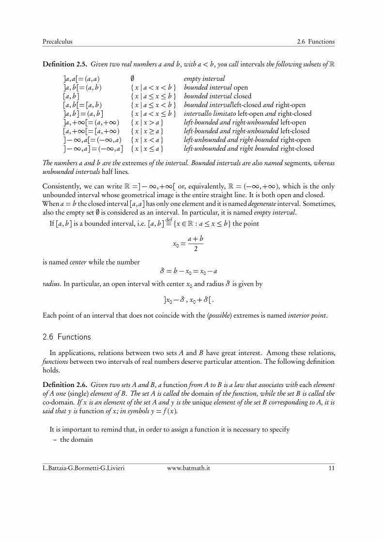
Definition 2.5. Given two real numbers a and b , with a < b , you call intervals the following subsets of R
]a,a[= (a,a) ; empty interval]a, b [= (a, b ) x | a < x < b bounded interval open[a, b ] x | a ≤ x ≤ b bounded interval closed[a, b [= [a, b ) x | a ≤ x < b bounded intervalleft-closed and right-open]a, b ] = (a, b ] x | a < x ≤ b intervallo limitato left-open and right-closed]a,+∞[= (a,+∞) x | x > a left-bounded and right-unbounded left-open[a,+∞[= [a,+∞) x | x ≥ a left-bounded and right-unbounded left-closed]−∞,a[= (−∞,a) x | x < a left-unbounded and right-bounded right-open]−∞,a] = (−∞,a] x | x ≤ a left-unbounded and right bounded right-closed
The numbers a and b are the extremes of the interval. Bounded intervals are also named segments, whereasunbounded intervals half lines.
Consistently, we can write R =]−∞,+∞[ or, equivalently, R = (−∞,+∞), which is the onlyunbounded interval whose geometrical image is the entire straight line. It is both open and closed.When a = b the closed interval [a,a] has only one element and it is named degenerate interval. Sometimes,also the empty set ; is considered as an interval. In particular, it is named empty interval.
If [a, b ] is a bounded interval, i.e. [a, b ] def= x ∈R : a ≤ x ≤ b the point
x0 =a+ b
2
is named center while the numberδ = b − x0 = x0− a
radius. In particular, an open interval with center x0 and radius δ is given by
]x0−δ , x0+δ[ .
Each point of an interval that does not coincide with the (possible) extremes is named interior point.
2.6 Functions
In applications, relations between two sets A and B have great interest. Among these relations,functions between two intervals of real numbers deserve particular attention. The following definitionholds.
Definition 2.6. Given two sets A and B, a function from A to B is a law that associates with each elementof A one (single) element of B. The set A is called the domain of the function, while the set B is called theco-domain. If x is an element of the set A and y is the unique element of the set B corresponding to A, it issaid that y is function of x; in symbols y = f (x).
It is important to remind that, in order to assign a function it is necessary to specify– the domain
L.Battaia-G.Bormetti-G.Livieri www.batmath.it 11
2 Sets, Numbers and Functions Precalculus
– the co-domain– a law that associates with the element x in the domain the unique element y in the co-domain.
Different notations are used to indicate a function. The most complete one is the following
f : A→ B , x 7→ f (x) ,
but, often, the symbolx 7→ f (x) ,
is used if the sets A and B have already been defined or their definition is clear from the context. However,the most used one is the less rigorous notation y = f (x) (to be read y is f of x).
Example 2.4. If A and B are the set of real numbers, we can consider the function that associates withthe real number x ∈A the element y = x2 in B . So, we can use one of the following three notations
f : R→R, x 7→ x2,
orx 7→ x2
ory = x2 .
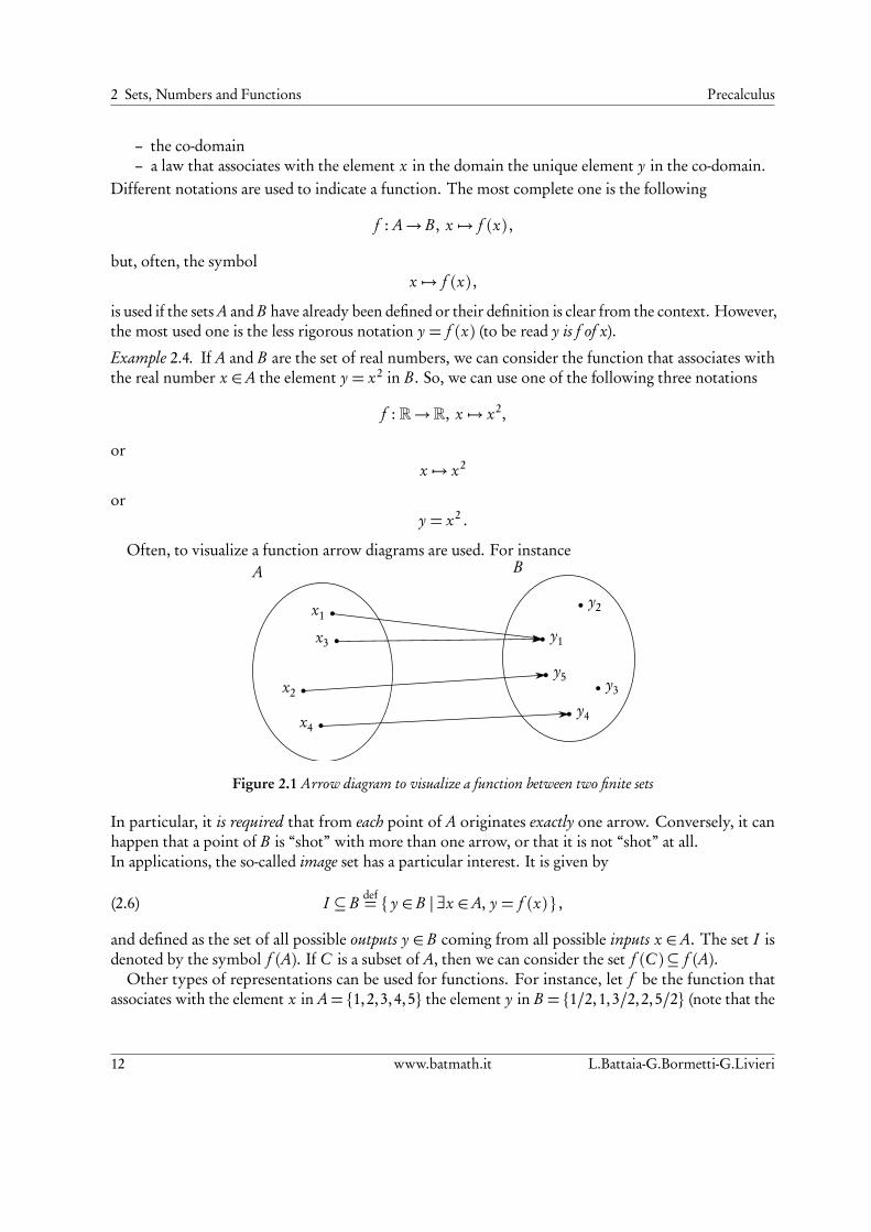
Often, to visualize a function arrow diagrams are used. For instance
bx4
bx1
bx2
bx3b y1
b y2
b y3
b y4
b y5
A B
Figure 2.1 Arrow diagram to visualize a function between two finite sets
In particular, it is required that from each point of A originates exactly one arrow. Conversely, it canhappen that a point of B is “shot” with more than one arrow, or that it is not “shot” at all.In applications, the so-called image set has a particular interest. It is given by
(2.6) I ⊆ B def= y ∈ B | ∃x ∈A, y = f (x) ,
and defined as the set of all possible outputs y ∈ B coming from all possible inputs x ∈A. The set I isdenoted by the symbol f (A). If C is a subset of A, then we can consider the set f (C )⊆ f (A).
Other types of representations can be used for functions. For instance, let f be the function thatassociates with the element x in A= 1,2,3,4,5 the element y in B = 1/2,1,3/2,2,5/2 (note that the
12 www.batmath.it L.Battaia-G.Bormetti-G.Livieri

Precalculus 2.6 Functions
domain of f is the subset of natural numbers 1,2,3,4,5, whereas the co-domain is the set of rationalnumbers). The following tabular representation can be used
x x/21 1/22 13 3/24 25 5/2
.
Table 2.1 Tabular representation of a function
In particular, in the first column there are the natural numbers 1, 2, . . . , 5 whereas in the second thecorresponding halves.
Another type of representation is the pie chart. For instance, let us consider an undergraduate programwhere 120 students, coming from different provinces, are enrolled:
Gorizia Pordenone Treviso Trieste Udine5 70 15 10 20.
To build the pie-chart, first we compute the percentages relative to each province
Gorizia Pordenone Treviso Trieste Udine4.17 58.33 12.5 8.33 16.67
,
then we map these percentages into the slices of the pie chart, taking into account that the whole piemeasures 360:
Gorizia Pordenone Treviso Trieste Udine15 210 45 30 60
At this point the chart is immediate
4.17 %Gorizia (5)
58.33 %
Pordenone (70)
12.5 %
Treviso (15)
8.33 %
Trieste (10)
16.67 %
Udine (20)
Figure 2.2 Pie-chart indicating the origin of 120 students enrolled in an undergraduate course
L.Battaia-G.Bormetti-G.Livieri www.batmath.it 13

2 Sets, Numbers and Functions Precalculus
Finally, a bar-chart it is also used
Gorizia Pordenone Treviso Trieste Udine
5
70
1510
20
Figure 2.3 Bar-chart indicating the origin of 120 students enrolled in an undergraduate course
As mentioned, we are mainly interested in numerical functions, where input and output variables arenumbers or groups of numbers. In particular, in this course real numbers come into play as variables,and for this reason we will talk about real functions of a real variable. In all these cases, we are dealingwith laws associating with a real number x one real number y only, so that they have a subset A of R asdomain and R as co-domain.In order to visualize the behaviour of a function, the study of its graph in an appropriate Cartesian planeturns out to be very useful. In particular, the following definition holds
Definition 2.7. The graph of a function f : A→ B is the set of pairs (x, y), with x ∈ A, y ∈ B, such thaty = f (x).
For instance, if we consider example in Table 2.1, we have to represent the points
A= (1, 1/2), B = (2,1), C = (3, 3/2), D = (4,2), E = (5, 5/2) ,
into the following graph:
1
2
3
1 2 3 4 5 6−1
bA
bB
bC
bD
bE
Figure 2.4 Cartesian graph
The graph in Figure 2.4 can be thought as a compacted arrow diagram.
14 www.batmath.it L.Battaia-G.Bormetti-G.Livieri
Precalculus 2.6 Functions
0.5
1.0
1.5
2.0
2.5
3.0
−0.51 2 3 4 5 6−1
A
B
C
D
E
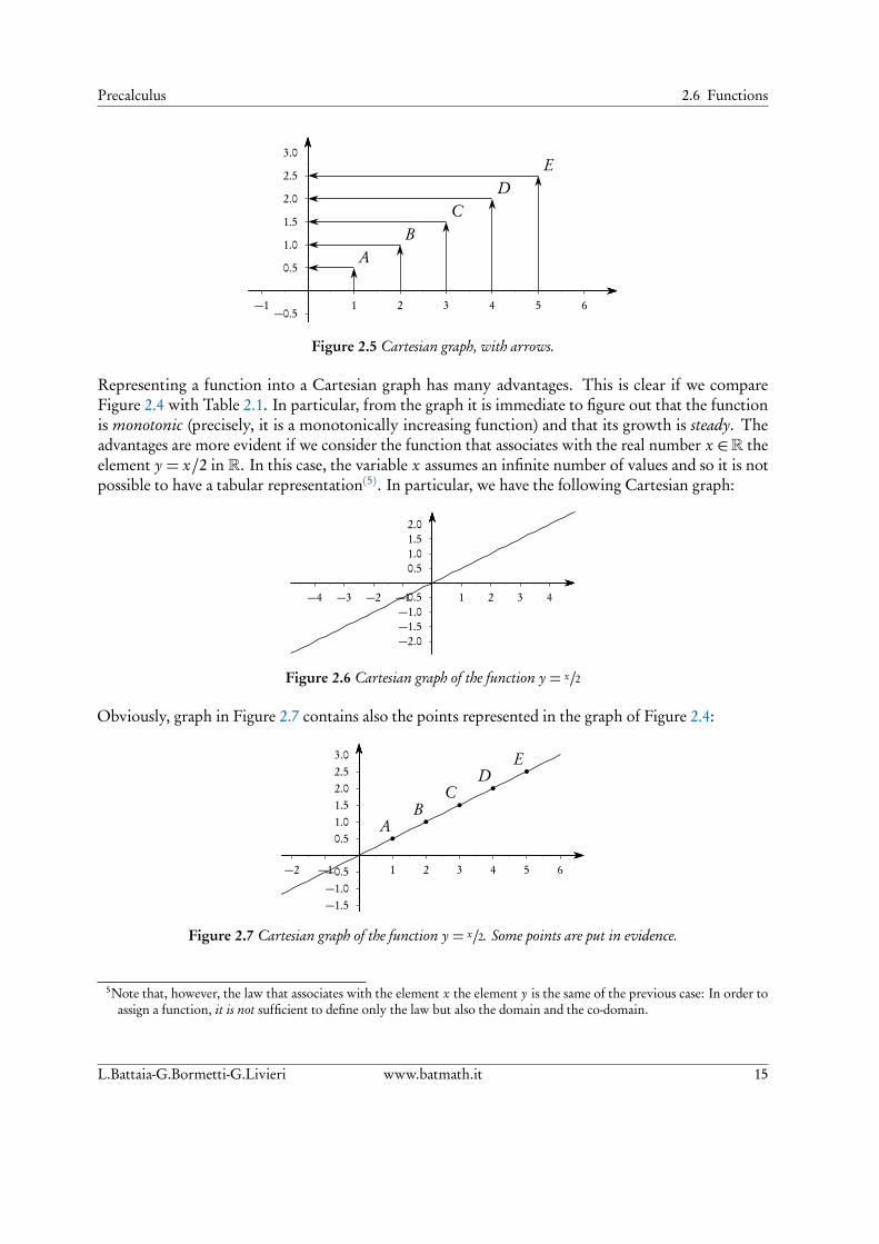
Figure 2.5 Cartesian graph, with arrows.
Representing a function into a Cartesian graph has many advantages. This is clear if we compareFigure 2.4 with Table 2.1. In particular, from the graph it is immediate to figure out that the functionis monotonic (precisely, it is a monotonically increasing function) and that its growth is steady. Theadvantages are more evident if we consider the function that associates with the real number x ∈R theelement y = x/2 in R. In this case, the variable x assumes an infinite number of values and so it is notpossible to have a tabular representation(5). In particular, we have the following Cartesian graph:
0.5
1.0
1.5
2.0
−0.5
−1.0
−1.5
−2.0
1 2 3 4−1−2−3−4
Figure 2.6 Cartesian graph of the function y = x/2
Obviously, graph in Figure 2.7 contains also the points represented in the graph of Figure 2.4:
0.5
1.0
1.5
2.0
2.5
3.0
−0.5
−1.0
−1.5
1 2 3 4 5 6−1−2
bA
bB
bC
bD
bE
Figure 2.7 Cartesian graph of the function y = x/2. Some points are put in evidence.
5Note that, however, the law that associates with the element x the element y is the same of the previous case: In order toassign a function, it is not sufficient to define only the law but also the domain and the co-domain.
L.Battaia-G.Bormetti-G.Livieri www.batmath.it 15
2 Sets, Numbers and Functions Precalculus
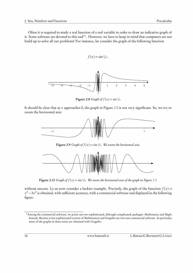
Often it is required to study a real function of a real variable in order to draw an indicative graph ofit. Some software are devoted to this end(6). However, we have to keep in mind that computers are notbuild up to solve all our problems! For instance, let consider the graph of the following function
f (x) = sin 1/x .
1 2 3 4 5−1−2−3−4−5
Figure 2.8 Graph of f (x) = sin 1/x
It should be clear that as x approaches 0, the graph in Figure 2.8 is not very significant. So, we try tozoom the horizontal axis:
1−1
Figure 2.9 Graph of f (x) = sin 1/x. We zoom the horizontal axis.
Figure 2.10 Graph of f (x) = sin 1/x. We zoom the horizontal axis of the graph in Figure 2.9.
without success. Le us now consider a luckier example. Precisely, the graph of the function f (x) =x3−3x2 is obtained, with sufficient accuracy, with a commercial software and displayed in the followingfigure.
6Among the commercial software, we point out two sophisticated, although complicated, packages: Mathematica and Maple.Instead, Maxima (a less sophisticated version of Mathematica) and Geogebra are two non commercial software. In particular,most of the graphs in these notes are obtained with Geogebra.
16 www.batmath.it L.Battaia-G.Bormetti-G.Livieri
Precalculus 2.7 Exercises
1
−1
−2
−3
−4
1 2 3−1−2−3
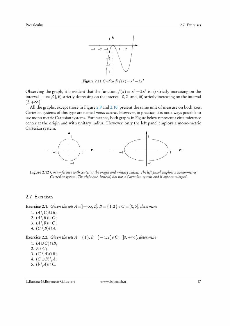
Figure 2.11 Grafico di f (x) = x3− 3x2
Observing the graph, it is evident that the function f (x) = x3 − 3x2 is: i) strictly increasing on theinterval ]−∞, 0], ii) strictly decreasing on the interval [0,2] and, iii) strictly increasing on the interval[2,+∞[.
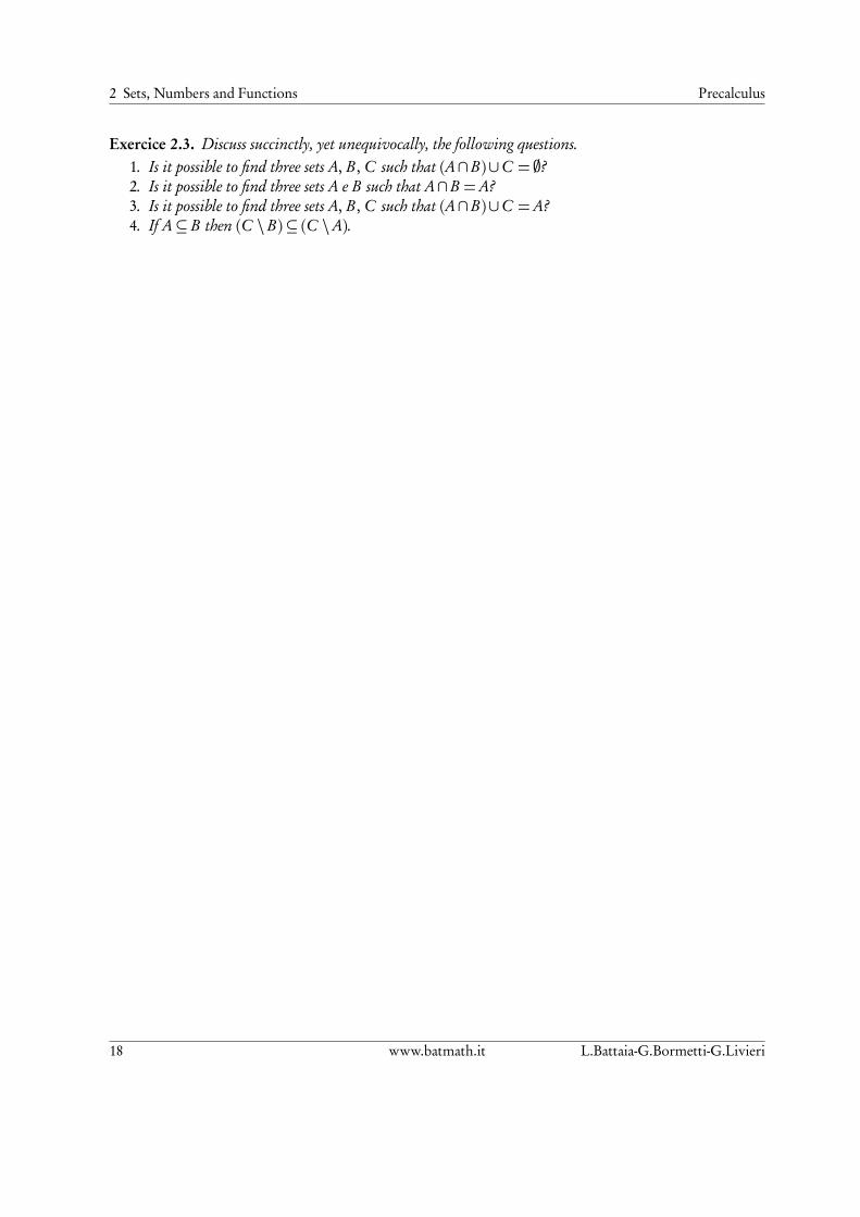
All the graphs, except those in Figure 2.9 and 2.10, present the same unit of measure on both axes.Cartesian systems of this type are named mono-metric. However, in practice, it is not always possible touse mono-metric Cartesian systems. For instance, both graphs in Figure below represent a circumferencecenter at the origin and with unitary radius. However, only the left panel employs a mono-metricCartesian system.
−1 1
1
−1
−1 1
1
−1
Figure 2.12 Circumference with center at the origin and unitary radius. The left panel employs a mono-metricCartesian system. The right one, instead, has not a Cartesian system and it appears warped.
2.7 Exercises
Exercice 2.1. Given the sets A=]−∞, 2], B = 1,2 e C = [0,5[, determine1. (A\C )∪B ;2. (A\B)∪C ;3. (A\B)∩C ;4. (C \B)∩A.
Exercice 2.2. Given the sets A= 1 , B =]− 1,2[ e C =]0,+∞[, determine1. (A∪C )∩B ;2. A\C ;3. (C \A)∩B ;4. (C ∪B) \A;5. (b \A)∩C .
L.Battaia-G.Bormetti-G.Livieri www.batmath.it 17
2 Sets, Numbers and Functions Precalculus
Exercice 2.3. Discuss succinctly, yet unequivocally, the following questions.1. Is it possible to find three sets A, B , C such that (A∩B)∪C = ;?2. Is it possible to find three sets A e B such that A∩B =A?3. Is it possible to find three sets A, B , C such that (A∩B)∪C =A?4. If A⊆ B then (C \B)⊆ (C \A).
18 www.batmath.it L.Battaia-G.Bormetti-G.Livieri
3 Equations
3.1 Linear equations
In this section we look at linear equations in one variable x.The most general linear equation – this means there will be no x2 terms and no x3’s, just x’s and numbers– in one variable is of the type
(3.1) ax = b , a 6= 0 .
Equation in (3.1) admits a unique solution(1)
(3.2) x =ba
.
If a ∈R, then three cases must be considered:– a 6= 0: the equation has only one solution x = b/a ;– a = 0∧ b 6= 0: the equation has no solution ;– a = 0∧ b = 0: the equation has an infinite number of solutions (basically all R).
In particular, it is important to consider the above conditions when solving parametric equations. Forinstance, consider the following example.
Example 3.1. Solve the following equation:
(a2− 1)x = a+ 1 .
To solve it, we have to take into account the following cases:– If a 6=±1, than it has only one solution x = (a+ 1)/(a2− 1)= 1/(a− 1) ;– If a = 1, than it has no solution;– If a =−1 , than it has an infinite number of real solutions.
The most general linear equation in two variables is of the type
(3.3) ax + b y = c , (a, b ) 6= (0,0) .
The condition on the parameters a and b is equivalent to say that they are not both zero at the sametime. Equation (3.3) has always an infinite number of solutions. To obtain these solutions one first
1The Fundamental Theorem of Algebra states that an equation of grade n has at maximum n solutions in R. As a consequenceequation (3.1) has always one solution. This is not the case if we consider non linear equations. For this type of equationsit is possible to have a number of solutions lower than the grade.
L.Battaia-G.Bormetti-G.Livieri www.batmath.it 19

3 Equations Precalculus
transforms equation (3.3) into a linear equation in one variable by fixing one of the two variables, thensolves the latter as previously discussed. For instance, the following equation
2x + 3y = 1
has as solutions the pairs (0, 1/3), (1/2, 0), (−1,1), etc.The following one variable equation, can be considered as a two variables equation where the coeffi-
cient of y is 0:3x = 1, or 3x + 0y = 1 ,
and it has as solutions the pairs (1/3, 1), (1/3, 2), (1/3,−5), etc.
3.2 Two dimensional systems of linear equations
In mathematics, a system of linear equations in two variables is a collection of two linear equationsinvolving the same set of variables. For example
(3.4)
ax + b y = pc x + d y = q ,
is a system of linear equations in the two variables x and y. The grade of the system is obtained as productof the grades of each equation. In particular, the system in Equation (3.4) has grade equal to one.
The word system indicates that equations have to be considered collectively, rather than individually.A solution to a linear system is an assignment of numbers to the variables such that all the equations aresimultaneously satisfied. In particular, the system is said
– determinate if it has a unique solution;– indeterminate if it has an infinite number of solutions;– inconsistent if it has no solution.
In general, a system of linear equations is consistent if there is at least one set of values for the unknownsthat satisfies every equation in the system.
Consider the following examples:
–
2x + y = 1x − y = 2
: The system is consistent and determinate. It has as unique solution the pair
(1,−1) .
–
x − 2y = 12x − 4y = 2
: The system is consistent and indeterminate. It has as solutions the pairs (2t +
1, t )∀t ∈R .
–
x − 2y = 12x − 4y = 3
: The system is inconsistent.
One method of solving a system of linear equations in two variables is the by substitution method. Themethod of solving by substitution works by solving one of the two equations (we choose which one)for one of the variables (we choose which one), and then plugging this back into the other equation,
20 www.batmath.it L.Battaia-G.Bormetti-G.Livieri

Precalculus 3.3 Second order equations
substituting for the chosen variable and solving for the other. Then we back-solve for the first variable.For instance
2x + y = 1x − y = 2
,
y = 1− 2xx − y = 2
,
y = 1− 2xx − (1− 2x) = 2
,
y = 1− 2xx = 1
,
y =−1x = 1
.
3.3 Second order equations
This section is about single-variable quadratic equations and their solutions.The most general quadratic equation is any equation having the form
(3.5) ax2+ b x + c = 0 , a 6= 0 ,
where x represents an unknown, and a, b , and c represent known numbers such that a is not equal to 0.If a = 0, then the equation is linear, not quadratic. A quadratic equation can be solved using the generalquadratic formula
(3.6) x1,2 =−b ±
pb 2− 4ac
2a.
In particular, it admits
– two distinct solutions if the quantity∆= b 2−4ac (named discriminant or simply Delta) is greaterthan zero;
– one solution (it is said that the quadratic equation has two coincident real solutions or that it has adouble solution) if∆= 0;
– no solution in R if∆< 0. In this case there are two solutions in the complex set C.
To fix ideas, we consider the following examples.
Examples.
– 2x2− 3x − 5= 0 =⇒ x1,2 =3±
p
9− 4 · 2(−5)2 · 2
=3±p
494
=
5/2−1
;
– x2− 6x + 9= 0 =⇒ x1,2 =6±p
36− 4 · 92
= 3;
– x2− 2x + 2= 0 =⇒ there is no solution because ∆= 4− 4 · 2< 0.
3.4 Higher order equations
There are general formulae for solving cubic (third degree polynomials) and quartic (fourth degreepolynomials) equations. However, we are not interested to them in this course. Instead, there are noformulae to solve general equations having grade greater than 4. We limit our analysis to two simplecases.
L.Battaia-G.Bormetti-G.Livieri www.batmath.it 21
3 Equations Precalculus
3.4.1 Elementary equations
An elementary equation is an equation of type
(3.7) axn + b = 0 , a 6= 0.
In order to solve Equation (3.7), we have to make the following steps: i) “take” the term b to the otherside of the equation (while changing the sign), ii) divide the latter term by a, iii) find the n-th root of theterm −b/a. It is important to make attention if n is an odd or an even number.
Example 3.2. 2x3+ 54= 0 =⇒ x3 =−27 =⇒ x =−3.
Example 3.3. 3x3− 12= 0 =⇒ x3 = 4 =⇒ x = 3p
4.
Example 3.4. 2x4+ 15= 0 =⇒ x4 =−15/2 =⇒ There is no solution.
Example 3.5. 3x4− 14= 0 =⇒ x4 = 14/3 =⇒ x =± 4p
14/3.
3.4.2 Factorizable equations
We only consider some example.
Example 3.6. x3− x2 = 0 =⇒ x2(x − 1) = 0 =⇒ x2 = 0∨ x − 1= 0 =⇒ x = 0∨ x = 1.
Example 3.7. x3−1= 0 =⇒ (x−1)(x2+x+1) = 0 =⇒ x = 1 only, as the equation x2+x+1= 0has no solution (∆< 0).
Example 3.8. x4−1= 0 =⇒ (x2−1)(x2+1) = 0 =⇒ (x−1)(x+1)(x2+1) = 0 =⇒ x =±1.(The equation x2+ 1= 0 has no solution).
3.5 Equations with radicals
A “radical” equation is an equation in which at least one variable expression is stuck inside a radical(in this course we consider the case of square roots or cubic roots).There is no standard technique to solve radical equations. In general, we solve equations by isolating thevariable. So, in the radical equation case we first have to isolate the square (or cubic) root, then to square(or to cube) both members. The new equation does not contain any radical. It is important to remindthat, in the square root case, we have to check if all the solutions of the new equation are consistentwith the initial one. There are no checks to do in the cubic root case. For instance
Example 3.9.p
x + 2+ x = 0,p
x + 2=−x, x + 2= x2, x2− x − 2= 0,
x1,2 =1±p
1+ 82
=
−12
, only the solution x = 1 is consistent.
Example 3.10.p
x + 2− x = 0,p
x + 2= x, x + 2= x2, x2− x − 2= 0,
x1,2 =1±p
1+ 82
=
−12
, only the solution x = 2 is consistent.
Example 3.11.p
1+ x2 = x+2, 1+ x2 = (x+2)2, 4x+3= 0, x =−3/4, the solution is consistent.
Example 3.12.p
2x2+ 1= 1− x, 2x2+ 1= (x + 2)2, 2x2+ 1= 1− 2x + x2, x2+ 2x = 0,x1 =−2, x2 = 0, both solutions are consistent.
22 www.batmath.it L.Battaia-G.Bormetti-G.Livieri
Precalculus 3.5 Equations with radicals
Example 3.13. 3p
x2− x − 1= x − 1, x2− x − 1= x3− 3x2+ 3x − 1, x3− 4x2+ 4x = 0, x(x2−4x + 4) = 0,x = 0∨ x = 2, both solutions are consistent.
L.Battaia-G.Bormetti-G.Livieri www.batmath.it 23

24 www.batmath.it L.Battaia-G.Bormetti-G.Livieri

4 Basic notions of Geometry
The aim of this chapter is to review some fundamental concepts of analytic geometry, also known ascoordinate geometry, or Cartesian geometry.
4.1 Cartesian coordinates
We start by considering the Cartesian product R×R×R=R3, i.e. the set of all ordered triples ofreal numbers. Thanks to the one-to-one correspondence between real numbers and points on a straightline, it is possible to represent the elements ofR3 as points on a space, which takes the name of Cartesianspace. In order to do so, we fix three oriented straights lines, which are called the Cartesian axes andusually are taken to be perpendicular to each other. In latter case, we speak about orthogonal Cartesianspace. Besides, if all the axes have the same unity of measure the Cartesian space is named mono-metric.In what follows, we always take into account mono-metric and orthogonal Cartesian spaces. The point(0,0,0) corresponds to the intersection point between the axes (called the origin). In this way, Cartesianaxes are indicated by Ox , Oy , Oz , or, simply x, y, z, and xy, x z, y z are named Cartesian planes.
Instead, if we consider the Cartesian plane R×R = R2, the Cartesian axis Ox is called horizontalaxis or axis of abscissae, whereas Oy vertical axis or axis of ordinates. The Cartesian plane is denotedby O xy and the Cartesian space by O xy z. Once the reference system O xy z is fixed, a one-to-onecorrespondence is set up between a point P in the space and an ordered triple of real numbers (thecoordinates of the point), as shown in Figure 4.1. In order to indicate the coordinates of the point P wewrite P (x, y, z) (P (x, y) into the plane) or, sometimes, P = (x, y, z) (P = (x, y) into the plane).
Ox
y
b
PP
b
xx
byy
x
y
z
b
P
xy
z
O
Figure 4.1 Cartesian coordinates of a point into the plane and into the space.
L.Battaia-G.Bormetti-G.Livieri www.batmath.it 25

4 Basic notions of Geometry Precalculus
4.2 Fundamental formulae of Geometry
Let A and B two points into the Cartesian space O xy, with respective coordinates (xA, yA) and (xB , yB ).The distance between A and B is given by
(4.1) AB =Æ
(xB − xA)2+(yB − yA)2 .
This formula is a direct consequence of the Pythagorean theorem, so the fact that we are working withan orthogonal Cartesian plane is crucial, as shown in Figure 4.2 below.
Ox
y
A
B
C
b
xAxA
b
xBxB
byAyA
byByB
AC = xC − xA= xB − xA
BC = yB − yC = yB − yA
Figure 4.2 Distance between two points and Pythagorean theorem
The midpoint M of the line segment joining the points A= (xA, yA) and B = (xB , yB ) has Cartesiancoordinates (xM , yM ) given by
(4.2) xM =xA+ xB
2, yM =
yA+ yB
2.
Finally, we report the formula for the centroid of a triangle. Precisely, given three vertices A= (xA, yA),B = (xB , yB ) and C = (xC , yC ) of a triangle ABC , the coordinates of the centroid G are given by
(4.3) xG =xA+ xB + xC
3, yG =
yA+ yB + yC
3.
4.3 Lines
The most general equation for a straight line into a Cartesian plane is given by
(4.4) ax + b y + c = 0
where a and b represent known numbers. In particular a and b cannot be equal to zero at the same time.In order to draw a line into a Cartesian plane it is sufficient to find out two solutions of Equation (4.4).
Example 4.1. Draw into the Cartesian plane the following line: 3x + 2y − 6 = 0. It is immediate toverify that the two points (0,3) and (2,0) satisfy the equation. The graph is the following:
26 www.batmath.it L.Battaia-G.Bormetti-G.Livieri

Precalculus 4.3 Lines
1
2
3
1 2 3 4 5−1−2−3
b A(0,3)
bB(2,0)
Figure 4.3 Line 3x + 2y − 6= 0
If b 6= 0, Equation (4.4) can be rewritten as
y =− ab
x − cb
,
or, setting m =− ab and q =− c
b , as
(4.5) y = mx + q .
The number m is the line’s slope (or gradient), whereas the number q is called vertical intercept. Forexample, the line in Figure (4.3) can be written as
y =−32
x + 3 ,
with m =−3/2 and q = 3. We observe that
(4.6) m =yB − yA
xB − xA.
The property in previous Equation (4.6) holds for any pair of points of the line. In particular, thenumerator yB − yA and the denominator xB − xA indicate, respectively, the vertical and the horizontalmovement done when moving from the point A to the point B . The line is: i) increasing, i.e. the slopem is positive, if it goes up from left to right, ii) decreasing, i.e. the slope m is negative, if it goes downfrom left to right, iii) horizontal, i.e. the slope m is zero, if it is a constant function. The usual formulafor the slope is the following one
(4.7) m =∆y∆x
,
where the difference yB−yA is indicated by∆y (it reads as delta y) and the difference xB−xA is indicated by∆x (it reads delta x). This is a very important notation and it is commonly used in practice. In particular,if we consider any variable g , then the difference between two values of g is named variation and it isdenoted by∆g . If∆g is positive (negative) we speak about increment (reduction) of g . For example, if
L.Battaia-G.Bormetti-G.Livieri www.batmath.it 27

4 Basic notions of Geometry Precalculus
the company Alfa has a gain g of 150.000$ for 2008 and of 180.000$ for 2009, then∆g = 30.000$. Inother words, the company has performed a gain of 30.000$ over one year.
Vertical lines are characterized by equations of type x = k, i.e. b = 0, while horizontal lines byequations the type y = k, i.e. m = 0. Besides, two non vertical lines are parallel if and only if they havethe same slope, whereas they are perpendicular if and only if the slope of the second line is the negativereciprocal of the slope of the first line, i.e. the product between their slopes is −1. In order to find out
the equation of a line, we can encounter the following situations.1. Line passing through a point P and known slope: If P (xP , yP ) is the point and m is the known slope,
than the equation of the line is
(4.8) y − yP = m(x − xP ) .
2. Line passing through two points A and B : if A(xA, yA) and B(xB , yB ) are two points, then theequation of the line is
(4.9) (x − xA)(yB − yA) = (y − yA)(xB − xA) .
Example 4.2. Determine the equation of the line s passing through (1,2) and parallel to the line r : 2x −y + 5= 0.
We first have to determine the slope of the line r . To do this, we write it into the form y = 2x − 5: itsslope is equal to 2. So, the equation of the line s is y − 2= 2(x − 1) (or, equivalently 2x − y = 0).
Example 4.3. Determine the equation of the line s passing through (2,1) and perpendicular to the liner : x − 2y − 1= 0.
We have: r : y = 1/2 x − 1/2. The slope of the line r is 12 . Hence, the slope of the line s will be −2 and so
the equation of the line is y − 1=−2(x − 2) (or, equivalently 2x + y − 5= 0).
Example 4.4. Determine the line passing through (2,3) and (4,−1).We immediately obtain (x − 2)(−1− 3) = (y − 3)(4− 2), which simplifies as 2x + y − 7= 0.
4.4 Parabolas
4.4.1 Parabola with vertical axis
The equation of a parabola with vertical axis is given by
(4.10) y = ax2+ b x + c , a 6= 0 ,
where a, b and c are known numbers, with a 6= 0. It has the following fundamental characteristics:
– If a > 0 its concavity is upward; if a < 0 its concavity is downward.– The vertex V has abscissa
(4.11) xV =−b2a
.
– The ordinate of V can be found by substituting the abscissa xV into the equation of the parabola.
28 www.batmath.it L.Battaia-G.Bormetti-G.Livieri
Precalculus 4.4 Parabolas
4.4.2 Parabola with horizontal axis
The equation of a parabola with horizontal axis is given by
(4.12) x = ay2+ b y + c , a 6= 0 .
where a, b and c are known numbers, with a 6= 0. It has the following fundamental characteristics:
– If a > 0 its concavity is rightward; if a < 0 its concavity is leftward.– The vertex V has ordinate
(4.13) yV =−b2a
.
– The abscissa of V can be found by substituting the ordinate yV into the equation of the parabola.
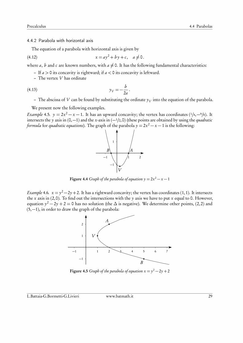
We present now the following examples.Example 4.5. y = 2x2 − x − 1. It has an upward concavity; the vertex has coordinates (1/4,−9/8). Itintersects the y axis in (0,−1) and the x-axis in (−1/2, 0) (these points are obtained by using the quadraticformula for quadratic equations). The graph of the parabola y = 2x2− x − 1 is the following:
1
−1
1 2−1
bA
bB
b
V
Figure 4.4 Graph of the parabola of equation y = 2x2− x − 1
Example 4.6. x = y2−2y+2. It has a rightward concavity; the vertex has coordinates (1,1). It intersectsthe x axis in (2,0). To find out the intersections with the y axis we have to put x equal to 0. However,equation y2 − 2y + 2 = 0 has no solution (the ∆ is negative). We determine other points, (2,2) and(5,−1), in order to draw the graph of the parabola:
1
2
−1
1 2 3 4 5 6 7−1
bV
bA
b
B
Figure 4.5 Graph of the parabola of equation x = y2− 2y + 2
L.Battaia-G.Bormetti-G.Livieri www.batmath.it 29

30 www.batmath.it L.Battaia-G.Bormetti-G.Livieri
5 Inequalities
A one-variable inequality is an expression of the type
f (x)Ñ g (x) (or, equivalently f (x)< g (x)∨ f (x)≤ g (x)∨ f (x)> g (x)∨ f (x)≥ g (x)),
while a two-variables inequality reads as
f (x, y)Ñ g (x, y) (or, equivalently f (x, y)< g (x, y)∨ f (x, y)≤ g (x, y)∨ f (x, y)< g (x, y)∨ f (x, y)≥ g (x, y)).
Solving an inequality means to find a range, or ranges, of values that the variable(s) can take and stillsatisfy the inequality.For instance, in the following examples
Example 5.1. – 3x2− 2x > 1: 2 is a solution; 0 is not a solution.– x2− 2y2 ≥ x + y: the pairs (2,0) is a solution; the pair (2,1) is not a solution.
It is important to note that, usually, in the one-variable inequalities case, there is an infinite numberof solutions which can be represented by using subsets of the real numbers (see Chapter 2, Paragraph2.5). Often, it is convenient to represent solutions graphically. This is because it is not always possibleto express the set of solutions in an analytical way.
5.1 First order inequalities
5.1.1 First order one-variable inequalities
A first order one-variable inequality assumes one of the following forms
(5.1) ax + b > 0, ax + b ≥ 0, ax + b < 0, ax + b ≤ 0 .
In general, it is convenient to consider the case a > 0, possibly changing the sign of both members.Attention: multiplying or dividing both sides of an inequality by the same negative number the sign of theinequality changes. To solve the inequality, then, one has first to isolate the variable, then to divide b bya. The following examples help to fix ideas.
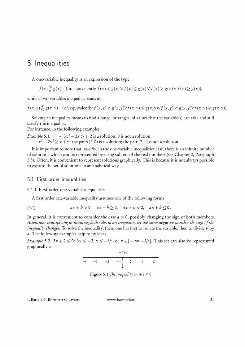
Example 5.2. 3x + 2 ≤ 0: 3x ≤ −2, x ≤ −2/3, or x ∈]−∞,−2/3]. This set can also be representedgraphically as
0 1 20−1−2−3−4
|
− 2/3
b
Figure 5.1 The inequality 3x + 2≤ 0
L.Battaia-G.Bormetti-G.Livieri www.batmath.it 31
5 Inequalities Precalculus
Example 5.3. 2x + 8 < 7x − 1: −5x < −9, 5x > 9, x > 9/5, or x ∈]9/5,+∞[. This set can also berepresented graphically as
0 1 2 3 4 50−1
|
9/5
Figure 5.2 The inequality 2x + 8< 7x − 1
Note 5.1. In Example (5.1), the point−2/3 is included into the set of solutions. In the second one, instead,the point 9/5 is not included. Usually a (small) filled circle is used to represent the first kind of points (itis possible to use other conventions. The important thing is to be clear and coherent.).
5.1.2 First order two-variable inequalities
A first order two-variable inequality always assumes one of the following forms
(5.2) ax + b y + c > 0, ax + b y + c ≥ 0, ax + b y + c < 0, ax + b y + c ≤ 0.
Equation ax + b y + c = 0 represents a line into the Cartesian plane. In particular, a line divides theplane in two half-planes. So, a first order two-variables inequality has as solution all the points in oneof the two half-planes. The points of the line belong to the set of solutions if the sign = appears intothe inequality. In order to know which of the two half-planes has to be selected, it is sufficient to takea point (not belonging to the line) in one of the two half-planes and check, numerically, if this pointsatisfies the inequality.
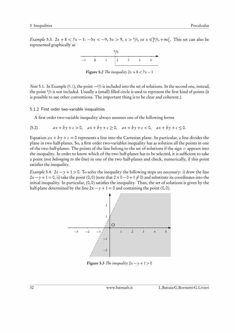
Example 5.4. 2x − y + 1> 0. To solve the inequality the following steps are necessary: i) draw the line2x− y+1= 0, ii) take the point (0,0) (note that 2×0−0+1 6= 0) and substitute its coordinates into theinitial inequality. In particular, (0,0) satisfies the inequality. Than, the set of solutions is given by thehalf-plane determined by the line 2x − y + 1= 0 and containing the point (0,0).
1
2
−1
−2
1 2 3 4 5−1−2−3
bO
Figure 5.3 The inequality 2x − y + 1> 0
32 www.batmath.it L.Battaia-G.Bormetti-G.Livieri

Precalculus 5.2 Inequalities of second order
Example 5.5. 2x + y + 1≥ 0. The set of solutions is represented by the following Figure 5.4:
1
2
−1
−2
1 2 3 4 5−1−2−3
bO
Figure 5.4 The inequality 2x + y + 1≥ 0
5.2 Inequalities of second order
5.2.1 One-variable second order inequalities
A second order one-variable inequality has the following representation
(5.3) ax2+ b x + c Ñ 0 .
The resolution method is very similar to the first-order case(1). Precisely, one first considers and drawsthe parabola y = ax2+ b x + c , then: i) if the sign of the inequality is ≥ the range of solutions is givenby the xs corresponding to the parts of the parabola which are above the x-axis; ii) if the sign of theinequality is≤ the range of solutions is given by the xs corresponding to the parts of the parabola whichare below the x-axis. The following examples will clarify the methodology.
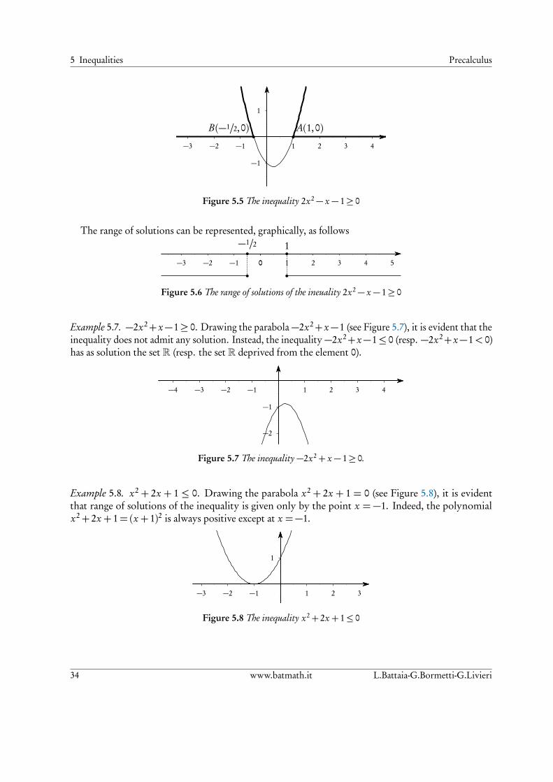
Example 5.6. 2x2− x − 1≥ 0. Drawing the parabola 2x2− x − 1 (see Figure 5.5), it is evident that therange of solutions of 2x2− x − 1≥ 0 are x ≤−1/2 or x ≥ 1, that is
x ∈
−∞,−12
∪ [1,+∞[.
1Actually there is a method that requires the study of the∆ of the quadratic equation ax2+ b x + c = 0, associated to theinequality.
L.Battaia-G.Bormetti-G.Livieri www.batmath.it 33
5 Inequalities Precalculus
1
−1
1 2 3 4−1−2−3
bA(1,0)
bB(−1/2, 0)
Figure 5.5 The inequality 2x2− x − 1≥ 0
The range of solutions can be represented, graphically, as follows
0 1 2 3 4 50−1−2−3
b1
b
−1/2
b b
Figure 5.6 The range of solutions of the ineuality 2x2− x − 1≥ 0
Example 5.7. −2x2+ x−1≥ 0. Drawing the parabola−2x2+ x−1 (see Figure 5.7), it is evident that theinequality does not admit any solution. Instead, the inequality−2x2+ x−1≤ 0 (resp. −2x2+ x−1< 0)has as solution the set R (resp. the set R deprived from the element 0).
−1
−2
1 2 3 4−1−2−3−4
Figure 5.7 The inequality −2x2+ x − 1≥ 0.
Example 5.8. x2 + 2x + 1 ≤ 0. Drawing the parabola x2 + 2x + 1 = 0 (see Figure 5.8), it is evidentthat range of solutions of the inequality is given only by the point x = −1. Indeed, the polynomialx2+ 2x + 1= (x + 1)2 is always positive except at x =−1.
1
1 2 3−1−2−3
Figure 5.8 The inequality x2+ 2x + 1≤ 0
34 www.batmath.it L.Battaia-G.Bormetti-G.Livieri

Precalculus 5.2 Inequalities of second order
5.2.2 Two-variable second-order inequalities
The resolution method is analogous to the case of the two-variable first order inequalities and thefollowing examples will clarify the procedure.
Example 5.9. x2+ y2− 2x − 2y + 1≤ 0. To solve this inequality the following steps are necessary: i)draw the circumference of equation x2+ y2− 2x− 2y+ 1= 0, ii) check if an internal point (for examplethe center) satisfies the inequality, then iii) if the center satisfies the inequality, the set of solutions isgiven by all the internal points and the points of the circumference (observe that the inequality is oftype “≤”).
1
2
1 2 3−1
bC
Figure 5.9 The inequality x2+ y2− 2x − 2y + 1≤ 0
Example 5.10. x2−y2
4< 1. Following the same procedure above and trying with the point (0,0), it is
possible to conclude that the inequality is verified by all the points between the two branches of the
hyperbola x2−y2
4= 1. However, in this case the sign of the inequality is <.
1
2
−1
−2
1 2 3−1−2−3
Figure 5.10 The inequality x2−y2
4< 1
L.Battaia-G.Bormetti-G.Livieri www.batmath.it 35

5 Inequalities Precalculus
5.3 Systems of inequalities
A system of inequalities is a set of inequalities in the same variables. Similarly to the systems ofequations case, a solution to a system of inequalities is an assignment of numbers to the variables suchthat all the inequalities are simultaneously satisfied. In this case, however, the graphical representationwill help significantly.
5.3.1 One-variable systems of inequalities
Example 5.11.
2x − 1≤ 0x2− 5x + 4> 0
. To solve the system it is necessary to solve separately each inequality.
The first has as solution x ≤ 1/2, while the second x < 1∨ x > 4. Drawing the graph in Figure 5.11, it iseasily to deduce that the solutions of the system are given by
−∞,12
.
0 1 2 3 4 5 6 70−1−2−3
|
1/2|
1|
4
b
Figure 5.11 Graphical representation of a one-variable system of inequalities
5.3.2 Two-variable systems of inequalities
The method of resolution is very similar to that presented in the previous section. One first solves,separately, each inequality of the system then one intersects the solutions. Also in this case, the graphicalrepresentation will be essential. We present the following example
Example 5.12.
x2+ y2− 2x > 0x − y − 2> 0
.
36 www.batmath.it L.Battaia-G.Bormetti-G.Livieri

Precalculus 5.4 Factorable polynomial inequalities
1
−1
−2
1 2 3 4 5−1−2−3
Figure 5.12 Graphical representation of a two-variable system of inequalities
The solution set is given by the chequered plane.
5.4 Factorable polynomial inequalities
Let suppose to have a one-variable or a two-variable inequality given by
f (x)Ñ 0, f (x, y)Ñ 0 .
and that the quantities f (x) or f (x, y) are not a first- or a second-order polynomials. In this case, the socalled rule of signs is used to solve the inequality. Basically the rule of signs states that the product of twonumbers with the same signs (resp. different signs) is positive (resp. negative). So, if the polynomialf (x) or f (x, y) is a factorable polynomial, in order to solve the inequality, one has first to determine thesign of each factor, then of the product. To facilitate the analysis, a graphical representation is used. Thefollowing examples will clarify the concepts.
Example 5.13. (x2−1)(x−2)> 0. The polynomial f (x) = (x2−1)(x−2)> 0 is a factorable polynomialwith factors (x2− 1) and (x − 2). In particular, the first factor, x2− 1, is positive for x <−1 and x > 1,negative for −1< x < 1, and zero for x =±1 (y = x2− 1 is the equation of a parabola). The secondfactor, x − 2 is positive for x > 2, negative for x < 2, and zero for x = 2. The conclusions are easilystated if we consider the graph in the following Figure 5.13
0 1 2 3 4 50−1−2−3−4−5
|
−1|
1|
2
bc bc
bc
bc bc bc− + − +
x2− 1
x − 2
Concl.
Figure 5.13 Graphical representation of the sign of the inequality (x2− 1)(x − 2)
Note that
L.Battaia-G.Bormetti-G.Livieri www.batmath.it 37
5 Inequalities Precalculus
– a plain line is used to indicate the parts where each factor is positive ;– a dotted line is used to indicate the parts where each factor is negative ;– a 0 is used to indicate the points where each factor is exactly equal to zero .
Summarising, the inequality is satisfied for
x ∈]− 1,1[∪ ]2,+∞[ .
Note that to solve the inequality (x2− 1)(x − 2)< 0 it is not necessary to construct a new graph. Inparticular, (x2− 1)(x − 2)< 0 is satisfied for
x ∈]−∞,−1[∪ ]1,2[.
Analogously, the inequalities (x2− 1)(x − 2)≤ 0 and (x2− 1)(x − 2)≥ 0 has as solutions
]−∞,−1] ∪ [1,2] ,
and[−1,1] ∪ [2,+∞[ ,
respectively.
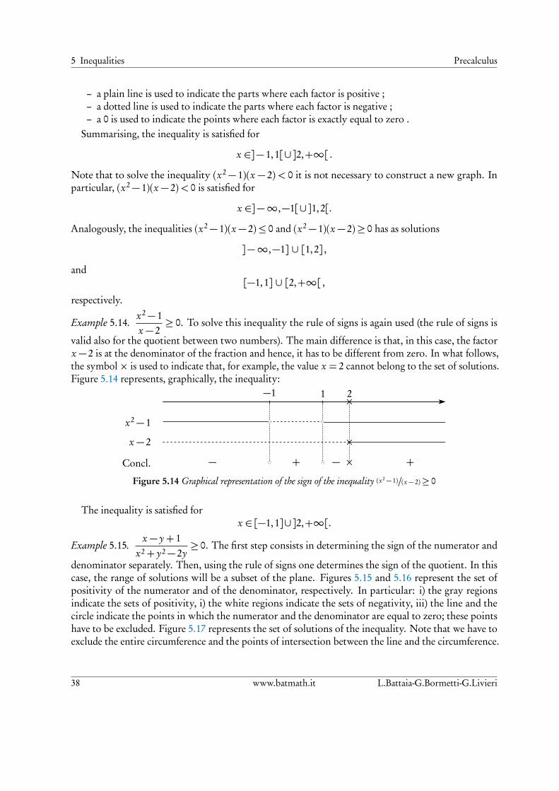
Example 5.14.x2− 1x − 2
≥ 0. To solve this inequality the rule of signs is again used (the rule of signs is
valid also for the quotient between two numbers). The main difference is that, in this case, the factorx − 2 is at the denominator of the fraction and hence, it has to be different from zero. In what follows,the symbol × is used to indicate that, for example, the value x = 2 cannot belong to the set of solutions.Figure 5.14 represents, graphically, the inequality:
|
−1|
1×
2
bc bc
×
bc bc ×− + − +
x2− 1
x − 2
Concl.
Figure 5.14 Graphical representation of the sign of the inequality (x2 − 1)/(x − 2)≥ 0
The inequality is satisfied forx ∈ [−1,1]∪ ]2,+∞[.
Example 5.15.x − y + 1
x2+ y2− 2y≥ 0. The first step consists in determining the sign of the numerator and
denominator separately. Then, using the rule of signs one determines the sign of the quotient. In thiscase, the range of solutions will be a subset of the plane. Figures 5.15 and 5.16 represent the set ofpositivity of the numerator and of the denominator, respectively. In particular: i) the gray regionsindicate the sets of positivity, i) the white regions indicate the sets of negativity, iii) the line and thecircle indicate the points in which the numerator and the denominator are equal to zero; these pointshave to be excluded. Figure 5.17 represents the set of solutions of the inequality. Note that we have toexclude the entire circumference and the points of intersection between the line and the circumference.
38 www.batmath.it L.Battaia-G.Bormetti-G.Livieri

Precalculus 5.5 Inequalities with radicals
1
2
−1
1 2−1−2
Figure 5.15 x − y + 1> 0
1
2
−1
1 2−1−2
Figure 5.16 x2+ y2− 2y > 0
1
2
−1
1 2 3−1−2−3−4
bc
bc
Figure 5.17x − y + 1
x2+ y2− 2y≥ 0
5.5 Inequalities with radicals
In this course only two types of inequalities with radicals are considered. In particular:
1.p
f (x)≥ g (x) (orp
f (x)> g (x));
2.p
f (x)≤ g (x) (orp
f (x)< g (x)).
To solve the first type, one has to consider the union of the solutions of the two systems
f (x)≥ 0g (x)< 0
∪
f (x)≥ g 2(x)g (x)≥ 0
,
or
f (x)≥ 0g (x)< 0
∪
f (x)> g 2(x)g (x)≥ 0
.
To solve the second type, instead, one has to consider the union of the solutions of the two systems:
f (x)≥ 0g (x)≥ 0f 2(x)≤ g (x)
,
or
f (x)≥ 0g (x)≥ 0f 2(x)< g (x)
.
Example 5.16.p
x2− 9x + 14> x − 8.
x2− 9x + 14≥ 0x − 8< 0
∪
x2− 9x + 14> (x − 8)2
x − 8≥ 0.
L.Battaia-G.Bormetti-G.Livieri www.batmath.it 39

5 Inequalities Precalculus
The first system is satisfied by x ≤ 2∨7≤ x < 8; the second system is satisfied by x ≥ 8. So, the range ofx values such that x ≤ 2∨ x ≥ 7 is the solution of
px2− 9x + 14> x − 8.
Example 5.17.p
4x2− 13x + 3< 2x − 3.
4x2− 13x + 3≥ 02x − 3≥ 04x2− 13x + 3< (2x − 3)2
.
Exercise
To solve a radical inequality containing only a radical with odd index root (in particular, with oddindex root equal to 3) it is sufficient to cube both members of the inequality and then, to solve the newinequality.
Example 5.18. 3p
x2+ 7> 2. If we cube both members, we obtain x2− 1> 0, which has as solutionsx <−1∨ x > 1.
5.6 Exercises
Exercice 5.1. Solve the following inequalities.1. x2+ 3x + 2> 0;
2. −x2− 3x + 2< 0;
3. 4− x2 > 0;
4. x2− x + 6< 0;
5. (x2+ 2x − 8)(x + 1)> 0;
6. (x2− 2)(x + 1)(1− x)≥ 0;
7. x(x2+ 2)(2x − 1)< 0;
8.x + 1x2+ 1
< 0;
9.2x − 8
1− x − x2> 0;
10.x2− 4x + 3
≤ 0;
11. x3− 27≥ 0;
12. 2− x3 < 0;
13. x3(x2− 1)(2− x2)≤ 0;
14.x − 9x3+ 1
≥ 0;
15.8− x3
x3+ 9≤ 0.
40 www.batmath.it L.Battaia-G.Bormetti-G.Livieri

Precalculus 5.6 Exercises
Exercice 5.2. Solve the following systems of inequalities.
1.
x2− 1> 02x + 3≥ 0
;
2.
x + 1> 0x2+ 2x − 8> 0
;
3.
x + 1< 0x2+ 1< 0
;
4.
2x − 8> 01− x − x2 < 0
;
5.
(1− 3x2)(x − 2)< 0(2+ x)(1− x)> 0
;
6.
3x − 2< 02x(3− x)> 0
;
7.
3x< 0
2x + 1x(2− 3x)
> 0;
8.
x − 3x
< 0
x + 11− x
> 0.
Exercice 5.3. Solve the following systems of inequalities.
1. 3
s
11− x
< 1;
2.
√
√
√ x3
x − 1> x + 1;
3.p
1− x2 < 1− x;
4.p
x < x;
5.p
1− x2 > x2;
6.p
x(x + 1)< 1− x.
Exercice 5.4. Determine, graphically, the solutions of the following systems of inequalities.
1.
y − x + 1> 02x − 3≤ 0
;
L.Battaia-G.Bormetti-G.Livieri www.batmath.it 41
5 Inequalities Precalculus
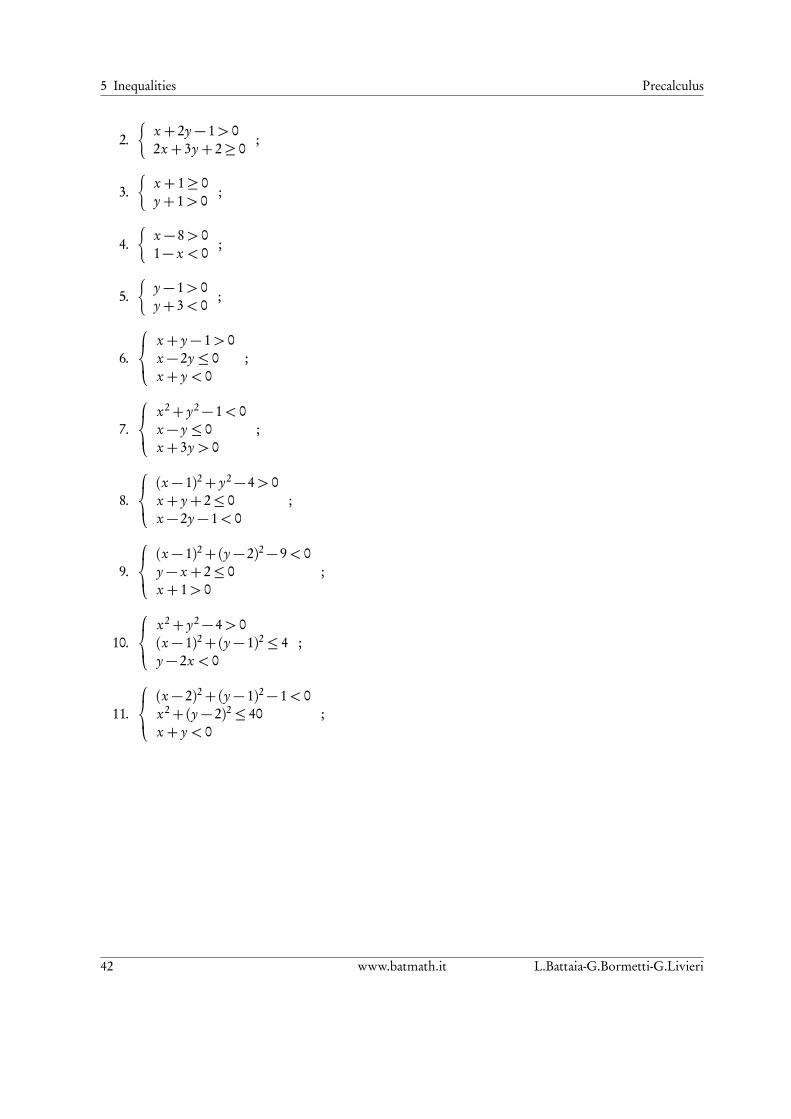
2.
x + 2y − 1> 02x + 3y + 2≥ 0
;
3.
x + 1≥ 0y + 1> 0
;
4.
x − 8> 01− x < 0
;
5.
y − 1> 0y + 3< 0
;
6.
x + y − 1> 0x − 2y ≤ 0x + y < 0
;
7.
x2+ y2− 1< 0x − y ≤ 0x + 3y > 0
;
8.
(x − 1)2+ y2− 4> 0x + y + 2≤ 0x − 2y − 1< 0
;
9.
(x − 1)2+(y − 2)2− 9< 0y − x + 2≤ 0x + 1> 0
;
10.
x2+ y2− 4> 0(x − 1)2+(y − 1)2 ≤ 4y − 2x < 0
;
11.
(x − 2)2+(y − 1)2− 1< 0x2+(y − 2)2 ≤ 40x + y < 0
;
42 www.batmath.it L.Battaia-G.Bormetti-G.Livieri
6 Exponentials and Logarithms
6.1 Powers
If a is any real number and m is a natural number greater or equal than 2, the power of base a andexponent m is given by the following number
(6.1) am = a · a · · ·a︸ ︷︷ ︸
m-times
.
If m = 1 and a is any real number, it is set, by definition,
(6.2) a1 = a .
Note that a1 is not a product: Two factors are needed to compute a product.If a is any real number different from zero, it is set, by definition
(6.3) a0 = 1 .
The expression 00 has no meaning. The power of base any real number a, different from zero, andexponent a negative integer number is given by
(6.4) a−m =1
am, a 6= 0.
Similarly to the Formula (6.3), the symbol 0negative.number has no meaning. It is also possible to define thepower of base a and exponent any real number. In this case, the base a has to be greater or equal thanzero if the exponent is not negative. If, instead, the exponent is a rational number of type m/n, with n anatural number greater than > 1, it is set, by definition,
(6.5) amn = np
am , a > 0 ; 0mn = 0,
mn> 0 .
The extension to the case of power of any real exponent (for example ap
2) is more complex and it isbeyond the purposes of this crash introduction. However, let describe the method in a specific case. Forinstance, let suppose that the problem is to compute a
p2. In this case, it is necessary to consider the
successive decimal approximation ofp
2 with an increasing number of decimal digits. In particular
1.4=1410
, 1.41=141100
, 1.414=14141000
, 1.4142=1414210000
, . . .
It is possible to compute a raised to each of the exponents that approximatep
2 because they are ratio-nal numbers. So, a
p2 will be the limit value of this sequence of numbers when the exponent tends to
p2.
L.Battaia-G.Bormetti-G.Livieri www.batmath.it 43
6 Exponentials and Logarithms Precalculus
Finally, the following properties hold (remind that the base has to be positive if the exponent is notan integer number, and different from zero if it appears in the denominator of a fraction)
(am)n = amn ;(6.6)am · an = am+n ;(6.7)
am
an= am−n .(6.8)
6.2 Power functions
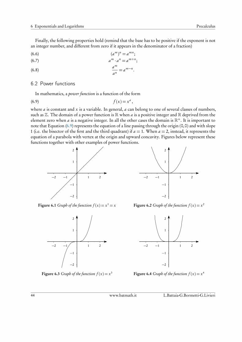
In mathematics, a power function is a function of the form
(6.9) f (x) = xa ,
where a is constant and x is a variable. In general, a can belong to one of several classes of numbers,such as Z. The domain of a power function is R when a is a positive integer and R deprived from theelement zero when a is a negative integer. In all the other cases the domain is R+. It is important tonote that Equation (6.9) represents the equation of a line passing through the origin (0,0) and with slope1 (i.e. the bisector of the first and the third quadrant) if a = 1. When a = 2, instead, it represents theequation of a parabola with vertex at the origin and upward concavity. Figures below represent thesefunctions together with other examples of power functions.
1
2
−1
−2
1 2−1−2
Figure 6.1 Graph of the function f (x) = x1 = x
1
2
−1
−2
1 2−1−2
Figure 6.2 Graph of the function f (x) = x2
1
2
−1
−2
1 2−1−2
Figure 6.3 Graph of the function f (x) = x3
1
2
−1
−2
1 2−1−2
Figure 6.4 Graph of the function f (x) = x4
44 www.batmath.it L.Battaia-G.Bormetti-G.Livieri

Precalculus 6.3 Exponential function
1
2
−1
−2
1 2−1−2
Figure 6.5 Graph of the function f (x) = x−1 = 1/x
1
2
−1
−2
1 2−1−2
Figure 6.6 Graph of the function f (x) = x−2 = 1/x2
1
2
−1
−2
1 2−1−2
Figure 6.7 Graph of the function f (x) = x1/2 =p
x
1
2
−1
−2
1 2−1−2
Figure 6.8 Graph of the function f (x) = 3p
x
Note 6.1. The function x1/3 is different from the function 3p
x. In particular, the first is defined forx ≥ 0, whereas the second ∀x ∈R. Besides, the graph of xa passes through the point (1,1) whichever isthe value of the exponent a.
Together with power functions, exponential and logarithmic functions are bricks used for building aconsiderable amount of mathematical models in many applications.
6.3 Exponential function
In mathematics, an exponential function is a function of the form
(6.10) f (x) = ax , a > 0 ,
where a, the base, is a positive real number different from 1 (the case a = 1 is not interesting because1x = 1, ∀x ∈R). The following figures report some examples of exponential functions.
L.Battaia-G.Bormetti-G.Livieri www.batmath.it 45

6 Exponentials and Logarithms Precalculus
1
2
1 2−1−2
Figure 6.9 Graph of the function f (x) = (1/2)x
1
2
1 2−1−2
Figure 6.10 Graph of the function f (x) = (1/3)x
1
2
1 2−1−2
Figure 6.11 Graph of the function f (x) = 2x
1
2
1 2−1−2
Figure 6.12 Graph of the function f (x) = 3x
Exponential functions are positive for each value of a and their graph passes through the point (0,1).A glance at Figures 6.9, 6.10, 6.11, 6.12 reveals that they are
1. Strictly increasing if a > 1 .2. Strictly decreasing if 0< a < 1 .
Besides, when a is greater than 1, the rate of growth of exponential functions is very large. Table 6.1clarifies this fact with an example.
x x2 2x
1 1 22 4 43 9 84 16 165 25 326 36 64
10 100 1024100 10000 ∼ 1.27 · 1030
Table 6.1 Comparison between x2 and 2x
There is a privileged base for exponential functions: The irrational Napier’s number e. Its value isapproximatively
e' 2.718 .
Because e> 1, the corresponding exponential function is increasing. In what follows, if not explicitlyspecified, the base e is always used and the related exponential function is denoted by exp(x).
46 www.batmath.it L.Battaia-G.Bormetti-G.Livieri
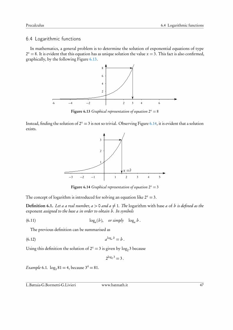
Precalculus 6.4 Logarithmic functions
6.4 Logarithmic functions
In mathematics, a general problem is to determine the solution of exponential equations of type2x = 8. It is evident that this equation has as unique solution the value x = 3. This fact is also confirmed,graphically, by the following Figure 6.13.
2
4
6
8
2 4 6−2−4−6 3
Figure 6.13 Graphical representation of equation 2x = 8
Instead, finding the solution of 2x = 3 is not so trivial. Observing Figure 6.14, it is evident that a solutionexists.
1
2
3
1 2 3 4 5−1−2−3
|x =?
Figure 6.14 Graphical representation of equation 2x = 3
The concept of logarithm is introduced for solving an equation like 2x = 3.
Definition 6.1. Let a a real number, a > 0 and a 6= 1. The logarithm with base a of b is defined as theexponent assigned to the base a in order to obtain b . In symbols
(6.11) loga(b ), or simply loga b .
The previous definition can be summarised as
(6.12) aloga b = b .
Using this definition the solution of 2x = 3 is given by log2 3 because
2log2 3 = 3 .
Example 6.1. log3 81= 4, because 34 = 81.
L.Battaia-G.Bormetti-G.Livieri www.batmath.it 47

6 Exponentials and Logarithms Precalculus
Example 6.2. log10 1000= 3, because 103 = 1000.
Example 6.3. log2116=−4, because 2−4 =
124=
116
.
Example 6.4. log10110=−1, because 10−1 =
110
.
Also for logarithmic functions, the most important base is the Napier’s number e. In what follows,to refer to logarithms with base e, the symbol ln (instead of loge), which stands for natural logarithm,is used. This notation is not universal. Sometimes, the natural logarithm is also denoted by log x. In thiscourse, instead, the notation log x is used to indicate the logarithm to the base 10 of x.:
(6.13) loge x = ln x .
The following properties hold
loga(xy) = loga x + loga y , x > 0, y > 0;(6.14)
loga
xy
= loga x − loga y , x > 0, y > 0;(6.15)
loga(x)y = y loga x , x > 0;(6.16)
loga a = 1 ;(6.17)loga 1= 0 .(6.18)
In particular, previous properties together with Formula (6.12) imply the following relations
(6.19) aloga x = x, ∀x > 0, loga ax = x, ∀x ∈R.
These relations indicate that the inverse of the logarithmic function is the exponential function and,conversely, the inverse of the exponential function is the logarithmic function.
Figures 6.15 and 6.16 report the graphics of the logarithmic function with base greater (Figure 6.15)and smaller (Figure 6.16) than 1, respectively. In particular, the same observations on monotonicitydone for exponential functions are valid.
1
2
−1
−2
1 2 3 4 5
Figure 6.15 Graph of the function log2 x
1
2
−1
−2
1 2 3 4 5
Figure 6.16 Graph of the function log1/2 x
48 www.batmath.it L.Battaia-G.Bormetti-G.Livieri
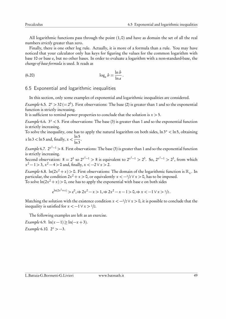
Precalculus 6.5 Exponential and logarithmic inequalities
All logarithmic functions pass through the point (1,0) and have as domain the set of all the realnumbers strictly greater than zero.
Finally, there is one other log rule. Actually, it is more of a formula than a rule. You may havenoticed that your calculator only has keys for figuring the values for the common logarithm withbase 10 or base e, but no other bases. In order to evaluate a logarithm with a non-standard-base, thechange-of-base-formula is used. It reads as
(6.20) loga b =ln blna
.
6.5 Exponential and logarithmic inequalities
In this section, only some examples of exponential and logarithmic inequalities are considered.
Example 6.5. 2x > 32 (= 25). First observations: The base (2) is greater than 1 and so the exponentialfunction is strictly increasing.It is sufficient to remind power properties to conclude that the solution is x > 5.
Example 6.6. 3x < 5. First observations: The base (3) is greater than 1 and so the exponential functionis strictly increasing.To solve the inequality, one has to apply the natural logarithm on both sides, ln3x < ln5, obtaining
x ln3< ln5 and, finally, x <ln5ln3
.
Example 6.7. 2x2−1 > 8. First observations: The base (3) is greater than 1 and so the exponential functionis strictly increasing.Second observation: 8 = 23 so 2x2−1 > 8 is equivalent to 2x2−1 > 23. So, 2x2−1 > 23, from whichx2− 1> 3, x2− 4> 0 and, finally, x <−2∨ x > 2.
Example 6.8. ln(2x2+ x)> 0. First observations: The domain of the logarithmic function is R+. Inparticular, the condition 2x2+ x > 0, or equivalently x <−1/2∨ x > 0, has to be imposed.To solve ln(2x2+ x)> 0, one has to apply the exponential with base e on both sides
eln(2x2+x) > e0,⇒ 2x2− x > 1,⇒ 2x2− x − 1> 0,⇒ x <−1∨ x > 1/2 .
Matching the solution with the existence condition x <−1/2∨ x > 0, it is possible to conclude that theinequality is satisfied for x <−1∨ x > 1/2.
The following examples are left as an exercise.
Example 6.9. ln(x − 1)≥ ln(−x + 3).
Example 6.10. 2x >−3.
L.Battaia-G.Bormetti-G.Livieri www.batmath.it 49

50 www.batmath.it L.Battaia-G.Bormetti-G.Livieri
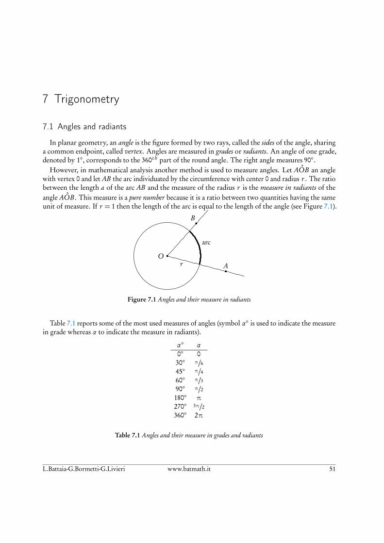
7 Trigonometry
7.1 Angles and radiants
In planar geometry, an angle is the figure formed by two rays, called the sides of the angle, sharinga common endpoint, called vertex. Angles are measured in grades or radiants. An angle of one grade,denoted by 1, corresponds to the 360t h part of the round angle. The right angle measures 90.
However, in mathematical analysis another method is used to measure angles. Let AOB an anglewith vertex 0 and let AB the arc individuated by the circumference with center 0 and radius r . The ratiobetween the length a of the arc AB and the measure of the radius r is the measure in radiants of theangle AOB . This measure is a pure number because it is a ratio between two quantities having the sameunit of measure. If r = 1 then the length of the arc is equal to the length of the angle (see Figure 7.1).
bO
bA
bB
arc
r
Figure 7.1 Angles and their measure in radiants
Table 7.1 reports some of the most used measures of angles (symbol α is used to indicate the measurein grade whereas α to indicate the measure in radiants).
α α0 030 π/645 π/460 π/390 π/2180 π270 3π/2360 2π
Table 7.1 Angles and their measure in grades and radiants
L.Battaia-G.Bormetti-G.Livieri www.batmath.it 51
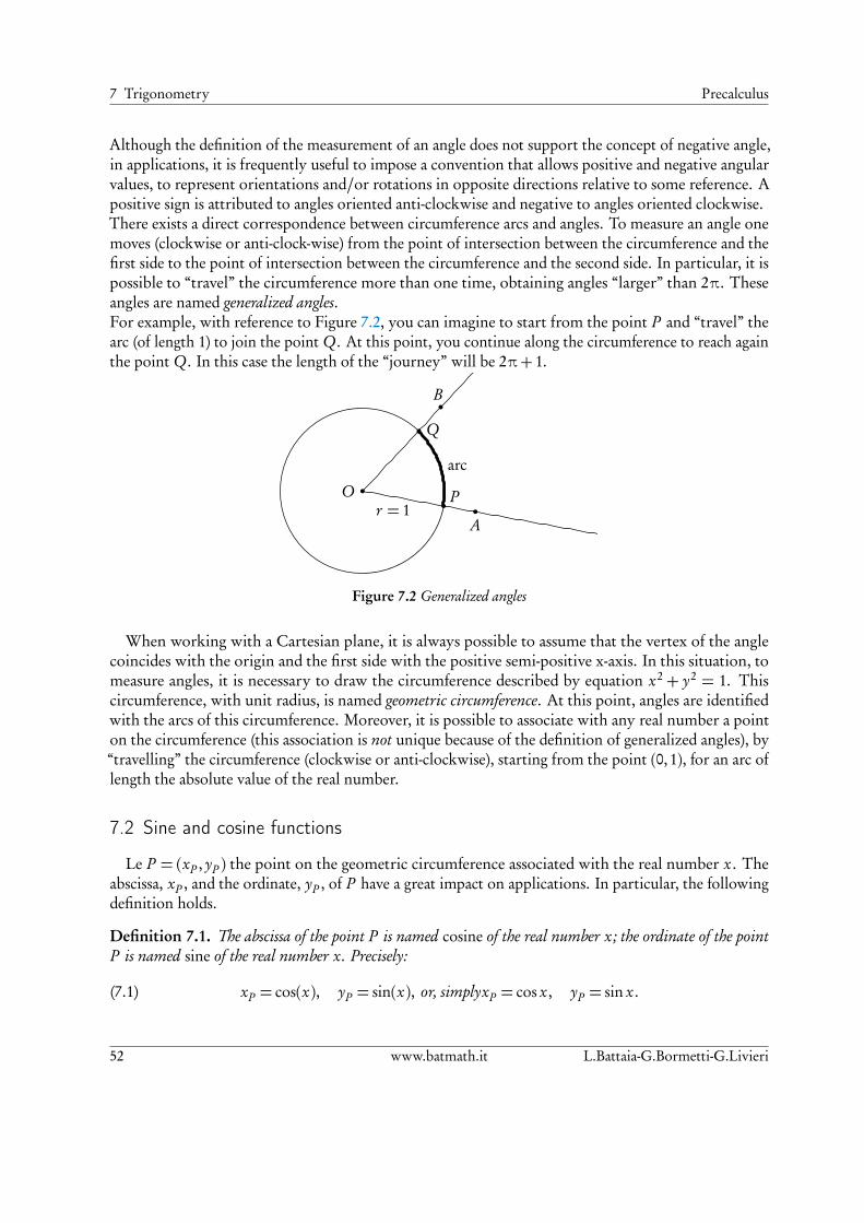
7 Trigonometry Precalculus
Although the definition of the measurement of an angle does not support the concept of negative angle,in applications, it is frequently useful to impose a convention that allows positive and negative angularvalues, to represent orientations and/or rotations in opposite directions relative to some reference. Apositive sign is attributed to angles oriented anti-clockwise and negative to angles oriented clockwise.There exists a direct correspondence between circumference arcs and angles. To measure an angle onemoves (clockwise or anti-clock-wise) from the point of intersection between the circumference and thefirst side to the point of intersection between the circumference and the second side. In particular, it ispossible to “travel” the circumference more than one time, obtaining angles “larger” than 2π. Theseangles are named generalized angles.For example, with reference to Figure 7.2, you can imagine to start from the point P and “travel” thearc (of length 1) to join the point Q. At this point, you continue along the circumference to reach againthe point Q. In this case the length of the “journey” will be 2π+ 1.
bOb
A
bB
arc
b P
b Q
r = 1
Figure 7.2 Generalized angles
When working with a Cartesian plane, it is always possible to assume that the vertex of the anglecoincides with the origin and the first side with the positive semi-positive x-axis. In this situation, tomeasure angles, it is necessary to draw the circumference described by equation x2 + y2 = 1. Thiscircumference, with unit radius, is named geometric circumference. At this point, angles are identifiedwith the arcs of this circumference. Moreover, it is possible to associate with any real number a pointon the circumference (this association is not unique because of the definition of generalized angles), by“travelling” the circumference (clockwise or anti-clockwise), starting from the point (0,1), for an arc oflength the absolute value of the real number.
7.2 Sine and cosine functions
Le P = (xP , yP ) the point on the geometric circumference associated with the real number x. Theabscissa, xP , and the ordinate, yP , of P have a great impact on applications. In particular, the followingdefinition holds.
Definition 7.1. The abscissa of the point P is named cosine of the real number x; the ordinate of the pointP is named sine of the real number x. Precisely:
(7.1) xP = cos(x), yP = sin(x), or, simplyxP = cos x, yP = sin x.
52 www.batmath.it L.Battaia-G.Bormetti-G.Livieri
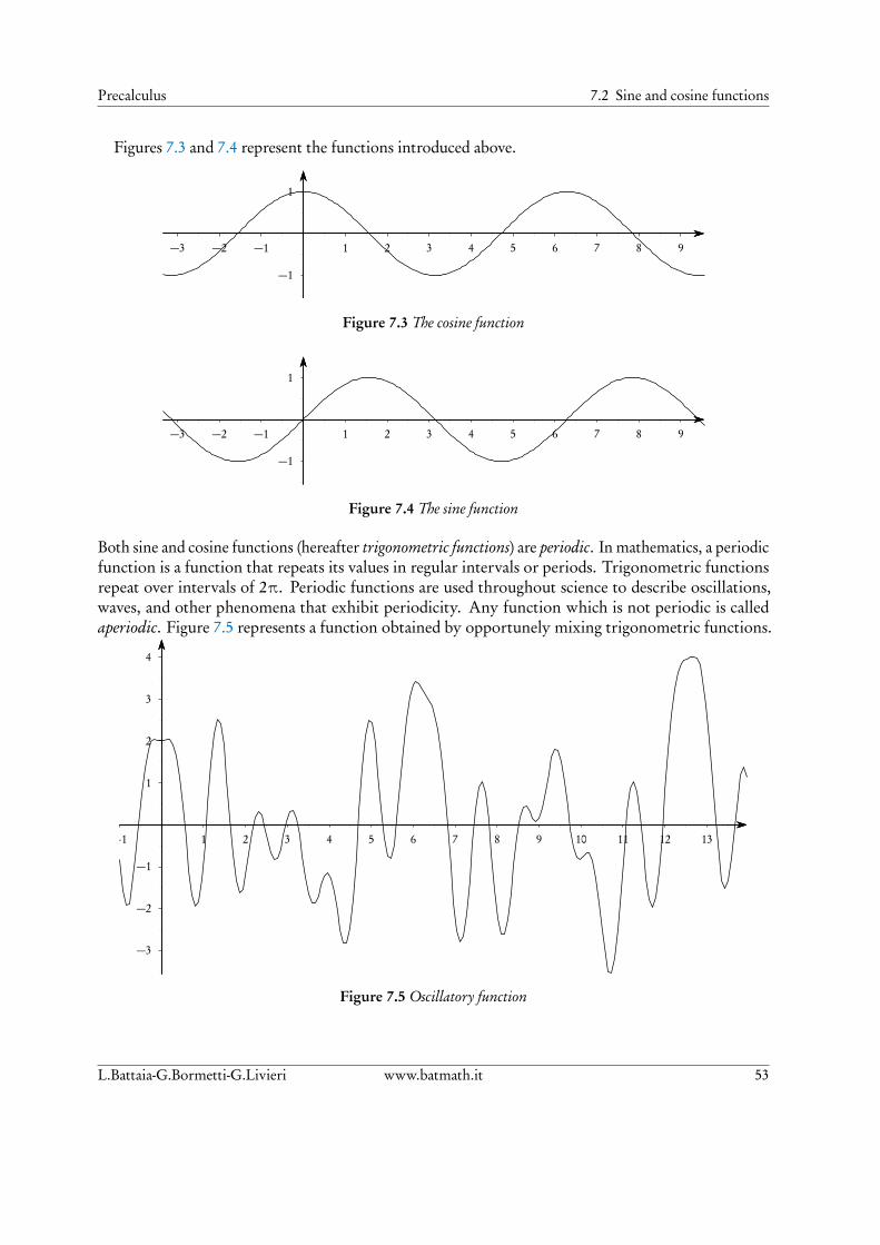
Precalculus 7.2 Sine and cosine functions
Figures 7.3 and 7.4 represent the functions introduced above.
1
−1
1 2 3 4 5 6 7 8 9−1−2−3
Figure 7.3 The cosine function
1
−1
1 2 3 4 5 6 7 8 9−1−2−3
Figure 7.4 The sine function
Both sine and cosine functions (hereafter trigonometric functions) are periodic. In mathematics, a periodicfunction is a function that repeats its values in regular intervals or periods. Trigonometric functionsrepeat over intervals of 2π. Periodic functions are used throughout science to describe oscillations,waves, and other phenomena that exhibit periodicity. Any function which is not periodic is calledaperiodic. Figure 7.5 represents a function obtained by opportunely mixing trigonometric functions.
1
2
3
4
−1
−2
−3
1 2 3 4 5 6 7 8 9 10 11 12 13−1
Figure 7.5 Oscillatory function
L.Battaia-G.Bormetti-G.Livieri www.batmath.it 53

7 Trigonometry Precalculus
7.3 Addition formulae
In this section some important formulae linked to trigonometric functions are given. In particular,the sum and difference formulae.
(7.2) cos(x ± y) = cos x cos y ∓ sin x sin y, sin(x ± y) = sin x cos y ± cos x sin y .
For instance, from
cosπ
4=p
22
, sinπ
4=p
22
, cosπ
6=p
32
, sinπ
6=
12
,
one obtains
cosπ
4− π
6
= cosπ
4cosπ
6+ sin
π
4sinπ
6=p
22
p3
2+p
22
12=p
6+p
24
.
In particular, setting x = y:
(7.3) cos(2x) = cos2 x − sin2 x , sin(2x) = 2sin x cos x .
54 www.batmath.it L.Battaia-G.Bormetti-G.Livieri
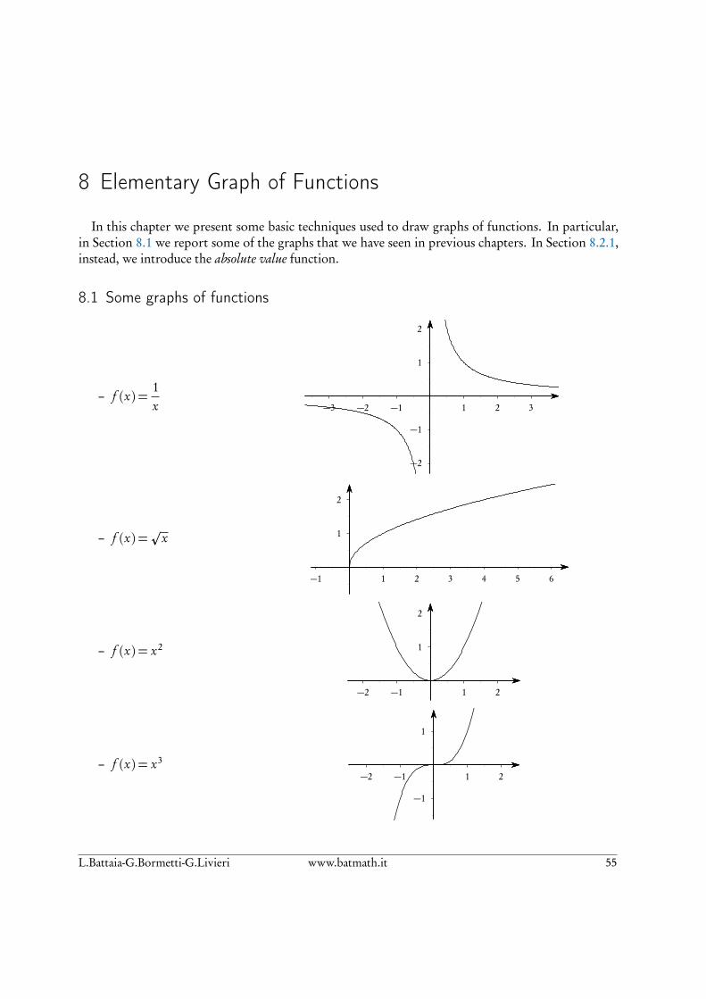
8 Elementary Graph of Functions
In this chapter we present some basic techniques used to draw graphs of functions. In particular,in Section 8.1 we report some of the graphs that we have seen in previous chapters. In Section 8.2.1,instead, we introduce the absolute value function.
8.1 Some graphs of functions
– f (x) =1x
1
2
−1
−2
1 2 3−1−2−3
– f (x) =p
x 1
2
1 2 3 4 5 6−1
– f (x) = x2 1
2
1 2−1−2
– f (x) = x3
1
−1
1 2−1−2
L.Battaia-G.Bormetti-G.Livieri www.batmath.it 55

8 Elementary Graph of Functions Precalculus
– f (x) = ex 1
2
1 2−1−2−3−4
– f (x) = ln(x)
1
2
−1
−2
1 2 3 4 5−1
– f (x) = sin(x)
1
−1
1 2 3 4 5 6 7
– f (x) = cos(x)
1
−1
1 2 3 4 5 6 7
8.2 Absolute value or modulus
8.2.1 Absolute value function
Definition 8.1. The non-negative real number defined by the formula
(8.1) |x|=
x, if x ≥ 0−x, if x < 0
.
is called the absolute value (or the modulus) of x.
The modulus of x thus represents the distance from the origin of the point on the real line with abscissax. The graph of the absolute value function, f (x) = |x|, is reported in Figure 8.1.
56 www.batmath.it L.Battaia-G.Bormetti-G.Livieri
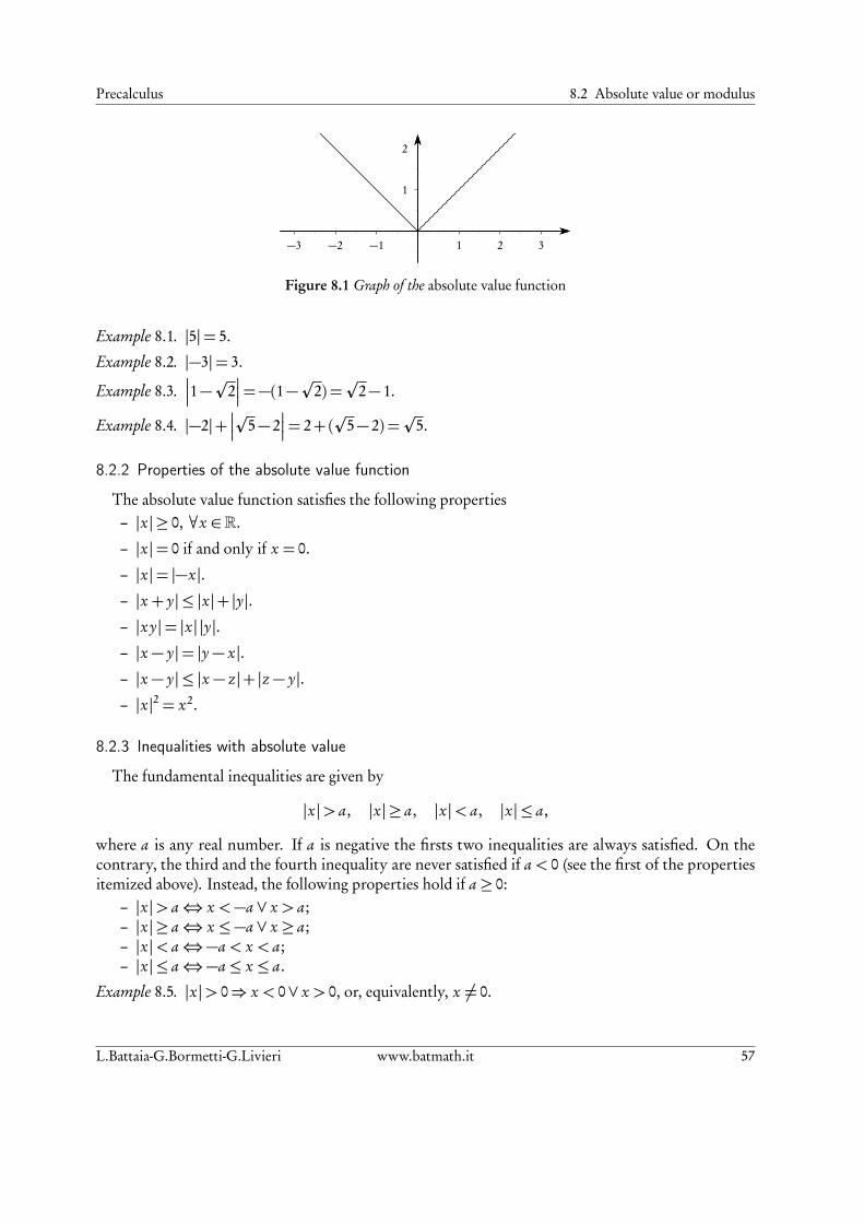
Precalculus 8.2 Absolute value or modulus
1
2
1 2 3−1−2−3
Figure 8.1 Graph of the absolute value function
Example 8.1. |5|= 5.
Example 8.2. |−3|= 3.
Example 8.3.
1−p
2
=−(1−p
2) =p
2− 1.
Example 8.4. |−2|+
p5− 2
= 2+(p
5− 2) =p
5.
8.2.2 Properties of the absolute value function
The absolute value function satisfies the following properties– |x| ≥ 0, ∀x ∈R.
– |x|= 0 if and only if x = 0.
– |x|= |−x|.– |x + y| ≤ |x|+ |y|.– |xy|= |x| |y|.– |x − y|= |y − x|.– |x − y| ≤ |x − z |+ |z − y|.– |x|2 = x2.
8.2.3 Inequalities with absolute value
The fundamental inequalities are given by
|x|> a, |x| ≥ a, |x|< a, |x| ≤ a,
where a is any real number. If a is negative the firsts two inequalities are always satisfied. On thecontrary, the third and the fourth inequality are never satisfied if a < 0 (see the first of the propertiesitemized above). Instead, the following properties hold if a ≥ 0:
– |x|> a⇔ x <−a ∨ x > a;– |x| ≥ a⇔ x ≤−a ∨ x ≥ a;– |x|< a⇔−a < x < a;– |x| ≤ a⇔−a ≤ x ≤ a.
Example 8.5. |x|> 0⇒ x < 0∨ x > 0, or, equivalently, x 6= 0.
L.Battaia-G.Bormetti-G.Livieri www.batmath.it 57
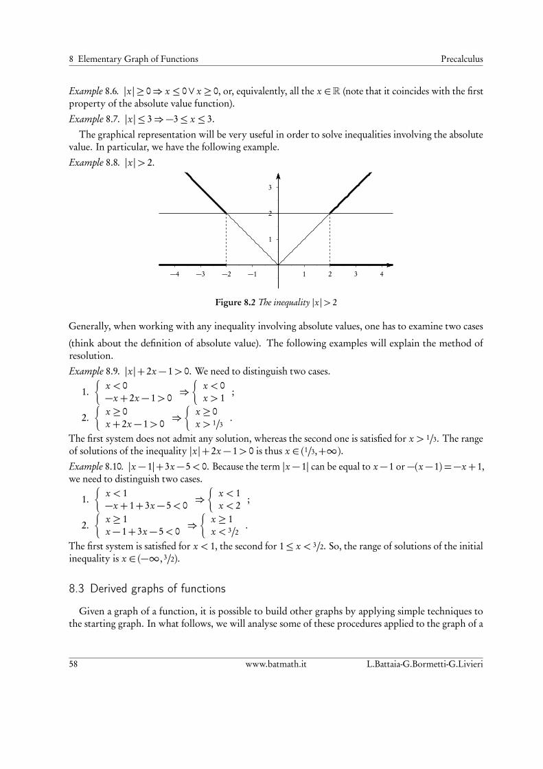
8 Elementary Graph of Functions Precalculus
Example 8.6. |x| ≥ 0⇒ x ≤ 0∨ x ≥ 0, or, equivalently, all the x ∈R (note that it coincides with the firstproperty of the absolute value function).
Example 8.7. |x| ≤ 3⇒−3≤ x ≤ 3.
The graphical representation will be very useful in order to solve inequalities involving the absolutevalue. In particular, we have the following example.
Example 8.8. |x|> 2.
1
2
3
1 2 3 4−1−2−3−4
Figure 8.2 The inequality |x|> 2
Generally, when working with any inequality involving absolute values, one has to examine two cases
(think about the definition of absolute value). The following examples will explain the method ofresolution.
Example 8.9. |x|+ 2x − 1> 0. We need to distinguish two cases.
1.
x < 0−x + 2x − 1> 0
⇒
x < 0x > 1
;
2.
x ≥ 0x + 2x − 1> 0
⇒
x ≥ 0x > 1/3
.
The first system does not admit any solution, whereas the second one is satisfied for x > 1/3. The rangeof solutions of the inequality |x|+ 2x − 1> 0 is thus x ∈ (1/3,+∞).Example 8.10. |x − 1|+3x−5< 0. Because the term |x − 1| can be equal to x−1 or −(x−1) =−x+1,we need to distinguish two cases.
1.
x < 1−x + 1+ 3x − 5< 0
⇒
x < 1x < 2
;
2.
x ≥ 1x − 1+ 3x − 5< 0
⇒
x ≥ 1x < 3/2
.
The first system is satisfied for x < 1, the second for 1≤ x < 3/2. So, the range of solutions of the initialinequality is x ∈ (−∞, 3/2).
8.3 Derived graphs of functions
Given a graph of a function, it is possible to build other graphs by applying simple techniques tothe starting graph. In what follows, we will analyse some of these procedures applied to the graph of a
58 www.batmath.it L.Battaia-G.Bormetti-G.Livieri

Precalculus 8.3 Derived graphs of functions
generic function as in Figure 8.3.
1
2
−1
1 2 3−1−2−3
Figure 8.3 Graph of a generic function f (x)
To get a better understanding, figures below report also, in dotted line, the graph of the initial functionof Figure 8.3.
Symmetry with respect to the x-axis: Wehave to change f (x) in − f (x).
1
−1
−2
1 2 3−1−2−3
Symmetry with respect to the y-axis: Wehave to change f (x) in f (−x).
1
2
−1
1 2 3−1−2−3
Horizontal translation to the left of k (>0) unities: We have to change f (x) inf (x + k).
1
−1
1 2 3−1−2−3
k
L.Battaia-G.Bormetti-G.Livieri www.batmath.it 59
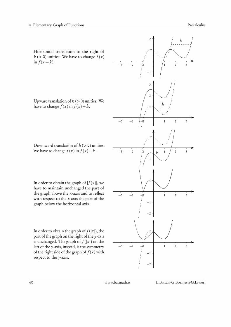
8 Elementary Graph of Functions Precalculus
Horizontal translation to the right ofk (> 0) unities: We have to change f (x)in f (x − k).
1
2
−1
1 2 3−1−2−3
k
Upward translation of k (> 0) unities: Wehave to change f (x) in f (x)+ k. 1
2
3
1 2 3−1−2−3
k
Downward translation of k (> 0) unities:We have to change f (x) in f (x)− k.
1
−1
1 2 3−1−2−3 k
In order to obtain the graph of | f (x)|, wehave to maintain unchanged the part ofthe graph above the x-axis and to reflectwith respect to the x-axis the part of thegraph below the horizontal axis.
1
−1
−2
1 2 3−1−2−3
In order to obtain the graph of f (|x|), thepart of the graph on the right of the y-axisis unchanged. The graph of f (|x|) on theleft of the y-axis, instead, is the symmetryof the right side of the graph of f (x)withrespect to the y-axis.
1
−1
−2
1 2 3−1−2−3
60 www.batmath.it L.Battaia-G.Bormetti-G.Livieri

Precalculus 8.3 Derived graphs of functions
It is also possible to combine the previous techniques in order to obtain other graphs.
Example 8.11. Draw the graph of the function f (x) = −p−x + 1. We start from the graph of the
function g (x) =p
x as in the second figure at Page 55. Then, we draw the graph ofp−x (symmetry
with respect to the y-axis) and, subsequently, of −p−x (symmetry with respect to the x-axis). Finally, we
draw the graph of −p−x + 1 (upward translation of k = 1 unity). Figures 8.4, 8.5 and 8.6 report the
just-described steps. Obviously, the graph of f (x) =−p−x + 1 can be also obtained by applying the
previous techniques in different order (note that f (x) =−p−x + 1=−(
p−x − 1).
1
−1−2−3−4
Figure 8.4 Graph of the functionp−x
−1
−1−2−3−4
Figure 8.5 Graph of the function −p−x
1
−1
1 2 3−1−2−3−4−5−6
Figure 8.6 Graph of the function −p−x + 1
Example 8.12. Draw the graph of f (x) =p−x − 1. In order to use the graphs previously drawn, it is
essential to rewrite f (x) =p−x − 1 as f (x) =
p
−(x + 1). So, in this case the sequence will be: i) drawpx, then ii)
p−x (see Figure 8.4) and, finally, iii)
p
−(x + 1) (see Figure 8.7).
1
2
1 2−1−2−3−4−5−6−7
Figure 8.7 Graph of the functionp−x − 1
Example 8.13. Draw the graph of f (x) = ln(|x − 1|). We start from the graph of ln x. Then, we drawthe graph of ln |x| (the graph on the left of the y-axis is the symmetric of the graph on the right of the vertical
L.Battaia-G.Bormetti-G.Livieri www.batmath.it 61

8 Elementary Graph of Functions Precalculus
axis) and, finally, of ln(|x − 1|) (horizontal translation to the right of k = 1 unity). Figures 8.8 and 8.9report the just-described steps.
1
−1
−2
1 2 3−1−2−3
Figure 8.8 Graph of the function ln |x|
1
−1
−2
1 2 3−1−2−3
Figure 8.9 Graph of the function ln |x − 1|
Example 8.14. Draw the graph of f (x) =1
|x| − 1. The sequence of steps required is: i) draw
1x
, then ii)
1x − 1
(horizontal translation to the right of k = 1 unity) and, finally iii)1
|x| − 1(the graph on the left of the
y-axis is the symmetric of the graph on the right of the vertical axis). Figures 8.10 and 8.11 report the lasttwo steps. We also report the lines of equation x = 1 and x =−1. In particular, these lines are namedasymptotes.
1
2
3
−1
−2
−3
1 2 3−1−2−3
Figure 8.10 Graph of the function 1/(x − 1)
1
2
3
−1
−2
−3
1 2 3−1−2−3
Figure 8.11 Graph of the function 1/(|x| − 1)
We note that it is not so difficult to deduce the domain and the image set from the graph of a function.Graphical representation of a function will also help to solve, graphically, a two-variable system ofequalities (see Paragraph 3.2 of chapter 3). We note that, in this case, the precise numerical value of thesolutions can be determined only approximatively.
62 www.batmath.it L.Battaia-G.Bormetti-G.Livieri
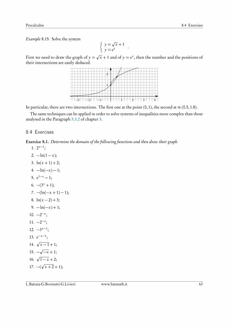
Precalculus 8.4 Exercises
Example 8.15. Solve the system
y =p
x + 1y = ex .
First we need to draw the graph of y =p
x + 1 and of y = ex , then the number and the positions oftheir intersections are easily deduced.
1
2
1 2 3 4−1−2−3
b
b
In particular, there are two intersections. The first one at the point (0,1), the second at ≈ (0.5,1.8).The same techniques can be applied in order to solve systems of inequalities more complex than those
analysed in the Paragraph 5.3.2 of chapter 5.
8.4 Exercises
Exercice 8.1. Determine the domain of the following functions and then draw their graph.1. 2x−1;
2. − ln(1− x);
3. ln(x + 1)+ 2;
4. − ln(−x)− 1;
5. e1−x − 1;
6. −(3x + 1);
7. −(ln(−x + 1)− 1);
8. ln(x − 2)+ 3;
9. − ln(−x)+ 1;
10. −2−x ;
11. −2−x ;
12. −3x−1;
13. e−x−1;
14.p
x − 1+ 1;
15. −p−x + 1;
16.p
1− x + 2;
17. −(p
x + 2+ 1);
L.Battaia-G.Bormetti-G.Livieri www.batmath.it 63

8 Elementary Graph of Functions Precalculus
18. −x2+ 2;
19. −(x − 2)2+ 3;
20. (1− x)3+ 2;
21. −(1− x)2+ 2;
22. −(x + 1)2− 2;
23. −x3+ 3.
Exercice 8.2. Determine the number of solutions of the following systems of equations.
1.
y = x3+ 1y = 2− (1− x)2 ;
2.
y = 1+(2− x)3
y =p
x + 1+ 2;
3.
y = ln(x − 1)+ 2y = 1−
px
;
4.
y = ex
y =−p
x + 2+ 3;
5.
y = e−x−1
y =p
x + 3;
6.
y = ln(x + 1)y =p
x;
7.
(
y =− ln(x + 1)
y =− 110
x;
8.
y = e−x + 3y = ln(x − 10) .
Exercice 8.3. Solve the following systems of inequalities.
1.
y + 3−x − 2> 0x2+ y2 < 4
;
2.
y − ln(1− x)+ 1> 0x2+ y2 ≥ 1
.
Exercice 8.4. Solve the following inequalities.1. |x|< 2;
2. |x + 1|> 3;
3.
x2− 1
< x;
4. |ex − 1|> 2;
64 www.batmath.it L.Battaia-G.Bormetti-G.Livieri
Precalculus 8.4 Exercises
5. |log2(x)− 1|< 2;
6. |x − 1|< 1.
Exercice 8.5. Given the function f (x) =−p−x + 1, determine first the image set, then the image of the
following sets1. A= [−3,2];
2. B =]− 2,−1[;
3. C = [0,1].
L.Battaia-G.Bormetti-G.Livieri www.batmath.it 65

66 www.batmath.it L.Battaia-G.Bormetti-G.Livieri
9 Sets and Functions: something more
9.1 Bounded and unbounded sets of real numbers
Attention: In this paragraph all the sets are subsets of the set R of the real numbers.
Definition 9.1. Let A⊆R be a set. A majorant of A is a real number x such that
(9.1) x ≥ a, ∀a ∈A.
A real number y is said minorant of A if
(9.2) y ≤ a, ∀a ∈A.
Example 9.1. Let A be the set A=]− 2,8]. Then −5, −π, −2 are minorants; 8, 10,p
89 are majorantsof A
Example 9.2. Let A be the set A=N. There are no majorants of A, while all the real numbers less orequal than zero are minorants of A.
Example 9.3. Let A be the set A=Z. There are no majorants and minorants of A.
Definition 9.2. Let A⊆R be a set. A is said to be bounded from above if it cannot extend indefinitelyrightwards on the real line, i.e., if there exists at least a majorant of A. Analogously, A is said to be boundedfrom below if it cannot extend indefinitely leftwards on the real line, i.e., if it there exists at least a minorantof A. A is said to be bounded if it is simultaneously bounded from above and from below.
Example 9.4. The set N is bounded from below but it is not bounded from above.
Example 9.5. The set Z is not bounded.
Example 9.6. The set A=]2,6[ is bounded.
Definition 9.3. A real number M is said to be the maximum (respectively, the minimum) of a set A⊆R if– M ∈A and– for every a ∈A one has a ≤M (respectively, a ≥M ).
The maximum (respectively, the minimum of a set) is unique.
Example 9.7. Consider the interval A = [0,1]. The maximum of A is 1, while the minimum is 0.Hereafter, we shall use the following notation for the maximum and the minimum of a set A: max(A)and min(A). In particular, 1=max(A) and 0=min(A).
Example 9.8. Let A be the set A=]0,1[. A has no maximum and no minimum.
Example 9.9. Let A be the set A=]0,1]. Then 1=max(A), whereas A has not minimum.
L.Battaia-G.Bormetti-G.Livieri www.batmath.it 67

9 Sets and Functions: something more Precalculus
Example 9.10. min(N) = 0, while N has not maximum.
Example 9.11. Z has no maximum and no minimum.
By definition, a set which is unbounded from above cannot have maximum and a set which isunbounded from below cannot have minimum. At the same time, it may happen that bounded setshave neither the maximum and the minimum. In particular, we give the following definition.
Definition 9.4. Let A ⊆ R a set bounded from above. The minimum of the majorants of A is namedsupremum of A and it is denoted by sup(A). Let now A be a set bounded from below. The maximum of theminorants of A is named infimum of A and it is denoted by inf(A). If A is an unbounded set form above,then, by definition, sup(A) = +∞; if A is an unbounded set from below, then, by definition, inf(A) =−∞.
Each subset of R has always a supremum (eventually +∞) and an infimum (eventually −∞). In orderto distinguish between bounded and unbounded sets, we name finite a supremum or infimum of boundedsets.
Example 9.12. +∞= sup(N), 0= inf(N) =min(N).
Example 9.13. +∞= sup(Z), −∞= inf(Z).
Example 9.14. 1= sup(]0,1[), 0= inf(]0,1[).
Example 9.15. 1= sup([0,1]) =max([0,1]), 0= inf([0,1]) =min([0,1]).
If a set has a maximum then the maximum is also a supremum of the set; similarly, if a set hasminimum then the minimum is also an infimum of the set. In particular, for a supremum and infimumof a set the following theorem holds.
Theorem 9.5. If A⊆R is a bounded set from above, then sup(A) satisfies the following properties1. sup(A)≥ a, ∀a ∈A;2. ∀ε > 0, ∃a ∈A, a > sup(A)− ε.
If A⊆R is a bounded set from below, then inf(A) satisfies the following properties1. inf(A)≤ a, ∀a ∈A;2. ∀ε > 0, ∃a ∈A, a < inf(A)+ ε.
9.2 Bounded and unbounded sets of the plane
The definition of bounded and unbounded set for a set A⊆R2 is different with respect to the definitionof bounded and unbounded set for a set A⊆R. This is because on the real line there exists an order.
Definition 9.6. Let A⊆R2 be a subset of the plane. A is said to be bounded if it is included into a circlewith center at the origin and radius r . Otherwise, it is said to be unbounded.
Example 9.16.
68 www.batmath.it L.Battaia-G.Bormetti-G.Livieri

Precalculus 9.3 Topology
A bounded set of the plane and a circlecontaining it.
1
2
−1
−2
1 2 3−1−2−3
Example 9.17.
An unbounded set of the plane: There areno circles containing it.
1
2
−1
−2
1 2 3−1−2−3
9.3 Topology
In what follows, we need to use similar concepts for subsets of the line and of the plane. In order tomake the definitions uniform, it is convenient to give the following
Definition 9.7. Let P be a point of the line (P is a real number) or of the plane (P is a pair of real numbers).A ball of radius ε and center P is the set of all points of distance less than ε from P; A closed ball of radius εand center P is the set of all points of distance less than or equal to ε away from P.
It is evident that on the line a ball is an interval (open or closed) of radius ε and center c ; on the plane aball is a circle (open if the circumference does not belong to the circle and close otherwise), of radius εand center at P .
Definition 9.8 (Neighbourhood). Given a point P in R or in R2, any open ball containing P is calledneighbourhood of P and it is denoted by I (P ) or IP .
We are particularly interested in neighbourhoods with center at P and radius ε. In particular, thelatters are denoted by I (P,ε).
L.Battaia-G.Bormetti-G.Livieri www.batmath.it 69
9 Sets and Functions: something more Precalculus
Definition 9.9 (Interior point). Let A be a set. A point P ∈A is called an interior point of A if there existsan open ball (i.e. a neighbourhood) centered at P that lies entirely in A. An interior point belongs to the set A.
Definition 9.10 (Exterior point). Let A be a set. A point P is called an exterior point of A if there exists aball (i.e. a neighbourhood) centered at P that lies entirely on the complementary set of A. An exterior pointdoes not belong to the set A.
Definition 9.11 (Isolated point). Let A be a set. A point P of A is called an isolated point of A if thereexists a neighbourhood I (P ) of P such that I (P )∩A= P, i.e., if P is an element of A but there exists aneighbourhood of P which does not contain any other point of A.
Definition 9.12 (Boundary point). Let A be a set. A point P is called a boundary point of A if for eachneighbourhood I (P ) of P it happens that I (P )∩A 6= ; and, contemporaneously, I (P )∩ ûA 6= ;, i.e. if in eachneighbourhood of P there exists at least a point of A and a point of the complementary set of A. A boundarypoint can belong or not belong to the set A.
Definition 9.13 (Accumulation point). Let A be a set. A point P is called an accumulation point of A ifin each neighbourhood I (P ) of P there exists an infinite number of points of A, i.e. the set I (P )∩A containsan infinite number of points. An accumulation point can belong or not belong to the set A.
We present now some examples.
Example 9.18. Let A= [0,2[∪5 be a subset of the line.– 1 is an interior point, because the neighbourhood I (1) =]1/2 , 3/2[ is all contained into A. The set
of all the interior points is given by ]0,2[.– 7 is an exterior point, because the neighbourhood I (5) =]6,8[ is all contained in the complemen-
tary set of A. The set of all the exterior points is given by ]−∞, 0[∪]2,5[∪[5,+∞[.– 5 is the only isolated point because the neighbourhood I (5) =]4,6[ intersected with A gives only
the point 5.– 0 is a boundary point because each neighbourhood of 0 contains points that do not belong to
A and points that belong to A. Similarly, 2 and 5 are boundary points. We note that 0,5 ∈A,while 2 /∈A.
– 1 is an accumulation point, because the neighbourhood I (1) =]1/2 , 3/2[ contains an infinite numberof points of A. Similarly, also 2 is an accumulation point. The set of all the accumulation points isgiven by [0,2].
We item now the following properties (suggestion: try to prove them as an exercise).– If P is an interior point than it is also an accumulation point;– If P is an interior point than it cannot be an isolated point or a boundary point;– If P is an isolated point than it is always a boundary point;– If P is an isolated point than it cannot be an accumulation point.
Example 9.19. In this example, the set A is given by union of the line r of equation x = 2, the pointP = (1,1) and the circle with center at the origin and radius 1. In particular, the semi-circumferencecontained on the half-plane y ≥ 0 belongs to the circle.The proof of the statements below is left as an exercise.
70 www.batmath.it L.Battaia-G.Bormetti-G.Livieri
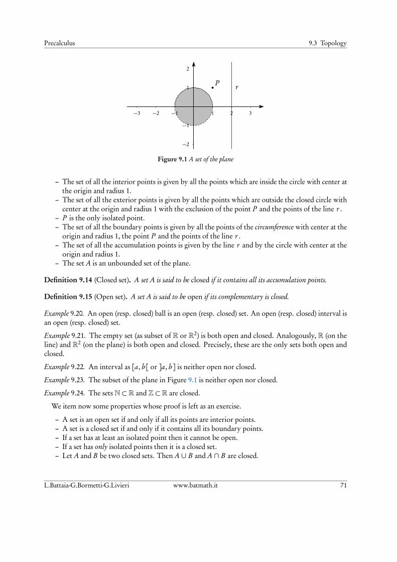
Precalculus 9.3 Topology
1
2
−1
−2
1 2 3−1−2−3
bP
r
Figure 9.1 A set of the plane
– The set of all the interior points is given by all the points which are inside the circle with center atthe origin and radius 1.
– The set of all the exterior points is given by all the points which are outside the closed circle withcenter at the origin and radius 1 with the exclusion of the point P and the points of the line r .
– P is the only isolated point.– The set of all the boundary points is given by all the points of the circumference with center at the
origin and radius 1, the point P and the points of the line r .– The set of all the accumulation points is given by the line r and by the circle with center at the
origin and radius 1.– The set A is an unbounded set of the plane.
Definition 9.14 (Closed set). A set A is said to be closed if it contains all its accumulation points.
Definition 9.15 (Open set). A set A is said to be open if its complementary is closed.
Example 9.20. An open (resp. closed) ball is an open (resp. closed) set. An open (resp. closed) interval isan open (resp. closed) set.
Example 9.21. The empty set (as subset of R or R2) is both open and closed. Analogously, R (on theline) and R2 (on the plane) is both open and closed. Precisely, these are the only sets both open andclosed.
Example 9.22. An interval as [a, b [ or ]a, b ] is neither open nor closed.
Example 9.23. The subset of the plane in Figure 9.1 is neither open nor closed.
Example 9.24. The sets N⊂R and Z⊂R are closed.
We item now some properties whose proof is left as an exercise.
– A set is an open set if and only if all its points are interior points.– A set is a closed set if and only if it contains all its boundary points.– If a set has at least an isolated point then it cannot be open.– If a set has only isolated points then it is a closed set.– Let A and B be two closed sets. Then A ∪ B and A ∩ B are closed.
L.Battaia-G.Bormetti-G.Livieri www.batmath.it 71
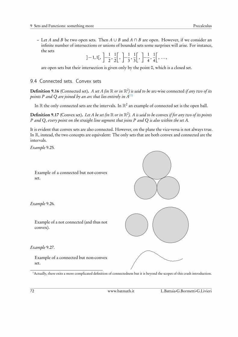
9 Sets and Functions: something more Precalculus
– Let A and B be two open sets. Then A ∪ B and A ∩ B are open. However, if we consider aninfinite number of intersections or unions of bounded sets some surprises will arise. For instance,the sets
]− 1,1[,
−12
,12
,
−13
,13
,
−14
,14
, . . . ,
are open sets but their intersection is given only by the point 0, which is a closed set.
9.4 Connected sets. Convex sets
Definition 9.16 (Connected set). A set A (in R or in R2) is said to be arc-wise connected if any two of itspoints P and Q are joined by an arc that lies entirely in A(1)
In R the only connected sets are the intervals. In R2 an example of connected set is the open ball.
Definition 9.17 (Convex set). Let A be set (inR or inR2). A is said to be convex if for any two of its pointsP and Q, every point on the straight line segment that joins P and Q is also within the set A.
It is evident that convex sets are also connected. However, on the plane the vice-versa is not always true.In R, instead, the two concepts are equivalent: The only sets that are both convex and connected are theintervals.
Example 9.25.
Example of a connected but not-convexset.
Example 9.26.
Example of a not connected (and thus notconvex).
Example 9.27.
Example of a connected but non-convexset.
1Actually, there exits a more complicated definition of connectedness but it is beyond the scopes of this crash introduction.
72 www.batmath.it L.Battaia-G.Bormetti-G.Livieri

Precalculus 9.5 Operations on functions
Example 9.28.
Example of a set which is convex and con-nected.
Example 9.29.
Example of a set which is convex and con-nected.
9.5 Operations on functions
In this section we suppose that the domain of the functions is a subset A of R or R2, whereas theco-domain is always the set R, i.e., we will work with one- or two-variable real functions. It is alwayspossible to sum, subtract or multiply two functions f and g ; besides, it is possible to divide two functionsonly if the second one is always different from zero.
Example 9.30. Let f (x) = |x| and g (x) = x2+ 1 be two real functions with domain R. Their sum is|x|+ x2+ 1, the difference is |x| − x2− 1, the product is |x| (x2+ 1) and, finally, the ratio is equal to|x|/(x2+ 1).
Example 9.31. If f (x) = ex and g (x) = x2, it is always possible to compute the sum and the product ofthese functions; however, to compute the ratio f/g , it is necessary to restrict the domain of the functiong to R \ 0.Under some conditions, it is possible to compose two functions f and g . Precisely, the functionsf :R→R and g :R→R can be composed to yield a function, which maps the point x in the domainof the function f to the point g ( f (x)) in the image of the function g . For example, if f (x) = x2 andg (x) = ex , then g ( f (x)) = ex2
.
Note 9.1. In order to compose two functions f and g , it is important that the image set of the functionf is a subset of the domain of the function g . For instance, if f (x) = x2− 1 and g (x) =
px, then we
must impose the condition x2− 1≥ 0.
9.6 Elementary functions and piecewise defined functions
In mathematics, an elementary function is a one- or two-variable function defined as the compositionof a finite number of arithmetic operations (+, −, ×, ÷), exponentials, logarithms, constants, andsolutions of algebraic equations. The most common way used to define non-elementary functions is toconstruct these functions “piece by piece”. Broadly speaking, we have to “combine” (the graphs of) twofunctions defined on different subsets of R (or R2).
L.Battaia-G.Bormetti-G.Livieri www.batmath.it 73

9 Sets and Functions: something more Precalculus
Example 9.32. Let f (x) =p
x and g (x) =p−x + 1 be two functions. The domain of the first function
is the range x ≥ 0, while the domain of the second one is x ≤ 1. Figures 9.2 and 9.3 report the graphs off and g , respectively.
1
2
1 2 3 4
Figure 9.2 Graph of the functionp
x
1
2
1 2−1−2−3−4
Figure 9.3 Graph of the functionp−x − 1
In what follows, we show how to construct other functions starting from f and g .
g (x) = p−x + 1, if x < 0px, if x ≥ 0
.1
2
1 2−1−2−3
h(x) = p−x + 1, if x < 1px, if x ≥ 1
.
1
2
1 2−1−2−3
k(x) = p−x + 1, if x < 0px, if x ≥ 1
.1
2
1 2−1−2−3
9.7 Domain of elementary functions
We have seen that in order to define a function (see 2.6, Page 11) it is necessary to specify i) its domain,ii) its co-domain, and iii) a law associating to each point on the domain a single point into the co-domain.The domain of an elementary function is the largest subset in which the operations to be executed onthe variables make sense. The following example will clarify this concept.
74 www.batmath.it L.Battaia-G.Bormetti-G.Livieri

Precalculus 9.8 Increasing and decreasing functions
Example 9.33. Determine the domain of f (x) =p
x − 1+ ln(2− x). To do so, we need to consider thefollowing system of equations
x − 1≥ 02− x > 0
,
Indeed, the domain of a radical function is given by the set of real numbers greater or equal than zero,while the domain of a logarithmic function is given by the set of positive real numbers. So, the domainof f is 1≤ x < 2.
Example 9.34. Determine the domain of f (x, y) =p
x2+ y2− 1. (Exercise)
9.8 Increasing and decreasing functions
Attention: The concepts of increasing and decreasing functions are meaningful only for one-variablefunctions.
Definition 9.18 (Increasing and decreasing functions). Let f : A→R be a one-variable function. If foreach pair of points x1 and x2 in A the condition x1 < x2 implies f (x1)≤ f (x2), then f is said to be weaklyincreasing (if, instead, x1 < x2 implies f (x1)< f (x2) then f is said to be strictly increasing). On the otherhand, if for each pair of points x1 and x2 in A the condition x1 < x2 implies f (x1)≥ f (x2), f is said to beweakly decreasing (if, instead, x1 < x2 implies f (x1)> f (x2) then f is said to be strictly decreasing).
The functions ex , ln x,p
x are strictly increasing functions; the function x2 is neither increasing nordecreasing. In particular, if a function is neither increasing nor decreasing, it is possible that it is piecewiseincreasing or piecewise decreasing. For instance, the function x2 is decreasing for x < 0 and increasingfor x > 0; the function 1/x is increasing for x < 0 and x > 0. In the latter case, however, we need to payattention on the domain.
9.9 Bounded and unbounded functions, maximum and minimum
The concepts of bounded and unbounded functions are linked to the image set of a function.
Definition 9.19 (Bounded and unbounded functions). If the whole graph of a function f , defined on adomain A, lies under some horizontal line of equation y =K, the function is said to be bounded from above.It means that
f (x)≤K ,
for each x ∈A. Similarly, f is said to be bounded from below if the graph has no points under some line ofequation y =H , i.e. if
f (x)≥H ,
for each x ∈A. A function which is bounded both from below and above is said to be bounded. A functionwhose image set is unbounded is said to be unbounded.
For instance, the trigonometric functions sin x and cos x are bounded, the function 1/x is unbounded,the function ex is bounded from below and the function −x2 is bounded from below.
We have seen that some points on the graph of f correspond to a maximum or minimum height.Now we give a precise definition for these type of points.
L.Battaia-G.Bormetti-G.Livieri www.batmath.it 75

9 Sets and Functions: something more Precalculus
Definition 9.20 (Maximum and minimum of a function). Let f be a function with domain A. A realnumber M is called the (global) maximum of f in A and P ∈A is called the (global) maximum point, if, foreach x ∈A,
M = f (P )≥ f (x).
Similarly, a real number m is called the (global) minimum of f in A and P ∈ A is called the (global)minimum point, if, for each x ∈A,
m = f (P )≤ f (x).
A maximum (or minimum) is said to be strict if the equal sign holds only for x = P. If the maximum andminimum of f do exist, than they are unique.
Finding the global maximum and minimum of a function is one of the most important application inoptimization problems.
For instance, the function ex has neither max nor min, its inf is 0 and its sup is +∞. The functionln x has neither max nor min, its inf is −∞ and its sup is +∞. The function sin x has 1 as max and −1as min. The function x2 has 0 as min, while it has not max; its sup is +∞.
Definition 9.21 (Relative maximum and minimum). Let f be a function with domain A. A point P ∈Ais said to be a relative maximum point if ∃I (P ) such that, for each point Q ∈ I (P ),
f (Q)≤ f (P ).
The point P is said to be a relative minimum point if
f (Q)≥ f (P ).
Relative maximum and minimum points may be many, and also infinitely many.
Example 9.35. The function represented in Figure 9.4 has x1 and x3 as relative maximum points, x2 andx4 as relative minimum points; it has not global minimum and maximum.
76 www.batmath.it L.Battaia-G.Bormetti-G.Livieri
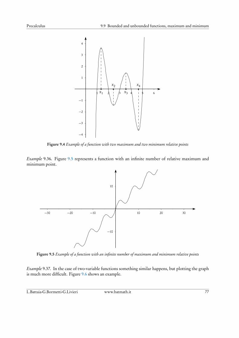
Precalculus 9.9 Bounded and unbounded functions, maximum and minimum
1
2
3
4
−1
−2
−3
−4
1 2 3 4 5 6
b
x1
b
x2b
x3
b
x4
Figure 9.4 Example of a function with two maximum and two minimum relative points
Example 9.36. Figure 9.5 represents a function with an infinite number of relative maximum andminimum point.
10
−10
10 20 30−10−20−30
Figure 9.5 Example of a function with an infinite number of maximum and minimum relative points
Example 9.37. In the case of two-variable functions something similar happens, but plotting the graphis much more difficult. Figure 9.6 shows an example.
L.Battaia-G.Bormetti-G.Livieri www.batmath.it 77

9 Sets and Functions: something more Precalculus
-2
0
2x
-2
0
2y
-0.5
0.0
0.5
1.0
z
Figure 9.6 Maximum and minimum points of a two-variable function
9.10 Injective, surjective and bijective functions
Definition 9.22. Let f : A→ B be a function. f is said to be i) injective if it never maps two distinctelements P1 and P2 of its domain to the same element of its co-domain, ii) surjective if every element of itsco-domain has a corresponding element in its domain , iii) bijective or a bijection if it is both injective andsurjective.
Example 9.38. The functions ex , ln x, x3,p
x are all injective functions.
Example 9.39. The functions ln x and x3, with co-domain R, are surjective functions. The functions ex
andp
x are surjective functions only if we restrict their co-domain to y > 0 and y ≥ 0, respectively.
Example 9.40. The real function f (x) = x3 is both injective and surjective.
Example 9.41. The functiom x2 is not injective. In particular, f (1) = f (−1) = 1.
9.11 Exercises
Exercice 9.1. Determine the characteristics (open, closed, bounded...) of the each of each set of solutions ofExercise 5.1, Page 40.
Exercice 9.2. Determine the characteristics of each set of solutions of Exercise 5.2, Page 41.
78 www.batmath.it L.Battaia-G.Bormetti-G.Livieri
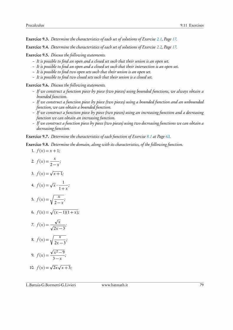
Precalculus 9.11 Exercises
Exercice 9.3. Determine the characteristics of each set of solutions of Exercise 2.1, Page 17.
Exercice 9.4. Determine the characteristics of each set of solutions of Exercise 2.2, Page 17.
Exercice 9.5. Discuss the following statements.– It is possible to find an open and a closed set such that their union is an open set.– It is possible to find an open and a closed set such that their intersection is an open set.– It is possible to find two open sets such that their union is an open set.– It is possible to find two closed sets such that their union is a closed set.
Exercice 9.6. Discuss the following statements.– If we construct a function piece by piece (two pieces) using bounded functions, we always obtain a
bounded function.– If we construct a function piece by piece (two pieces) using a bounded function and an unbounded
function, we can obtain a bounded function.– If we construct a function piece by piece (two pieces) using an increasing function and a decreasing
function we can obtain an increasing function.– If we construct a function piece by piece (two pieces) using two decreasing functions we can obtain a
decreasing function.
Exercice 9.7. Determine the characteristics of each function of Exercise 8.1 at Page 63.
Exercice 9.8. Determine the domain, along with its characteristics, of the following function.1. f (x) = x + 1;
2. f (x) =x
2− x;
3. f (x) =p
x + 1;
4. f (x) =p
x · 11+ x
;
5. f (x) =È x
2− x;
6. f (x) =p
(x − 1)(1+ x);
7. f (x) =p
xp
2x − 3;
8. f (x) =È x
2x − 3;
9. f (x) =p
x2− 93− x
;
10. f (x) =p
2xp
x + 3;
L.Battaia-G.Bormetti-G.Livieri www.batmath.it 79

9 Sets and Functions: something more Precalculus
11. f (x) =p
x + 1− x +p
2− x.
Exercice 9.9. Determine the characteristics of each set of solutions of Exercise 8.3, Page 64.
Exercice 9.10. Determine the domain, along with its characteristics, of the following functions.
1. f (x, y) =x
2− y;
2. f (x, y) =p
(x + 1)(y + 1);
3. f (x, y) =p
x · 11+ y
;
4. f (x, y) =È y
1+ x;
5. f (x, y) =p
(x2− 1)(2− y);
6. f (x, y) =pxy;
7. f (x, y) =p
x2− 4y + 3
;
8. f (x, y) =p
2xp
2y − 3;
9. f (x, y) =p
x + y − 1−px − y.
80 www.batmath.it L.Battaia-G.Bormetti-G.Livieri
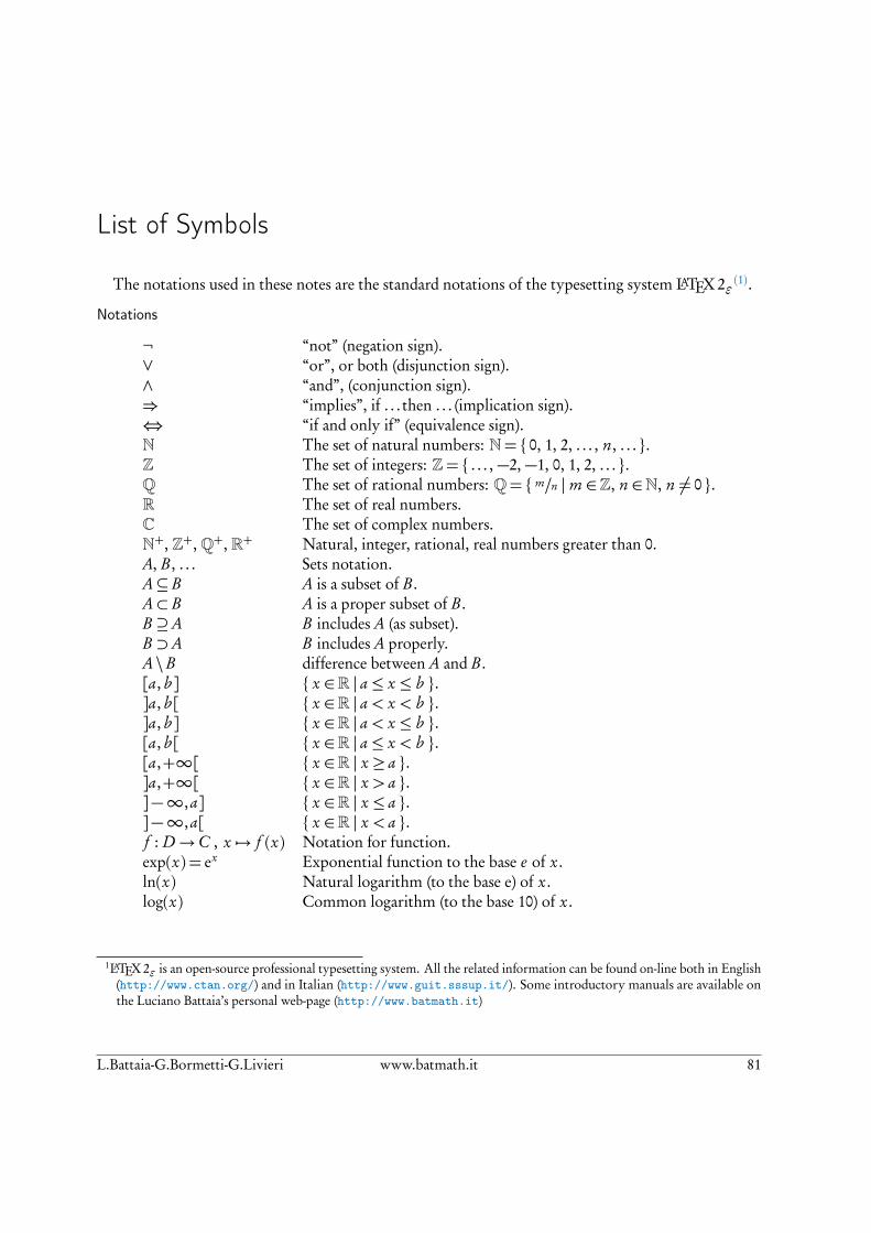
List of Symbols
The notations used in these notes are the standard notations of the typesetting system LATEX 2ε(1).
Notations
¬ “not” (negation sign).∨ “or”, or both (disjunction sign).∧ “and”, (conjunction sign).⇒ “implies”, if . . . then . . . (implication sign).⇔ “if and only if” (equivalence sign).N The set of natural numbers: N= 0, 1, 2, . . . , n, . . . .Z The set of integers: Z= . . . , −2, −1, 0, 1, 2, . . . .Q The set of rational numbers: Q= m/n | m ∈Z, n ∈N, n 6= 0 .R The set of real numbers.C The set of complex numbers.N+, Z+,Q+, R+ Natural, integer, rational, real numbers greater than 0.A, B , . . . Sets notation.A⊆ B A is a subset of B .A⊂ B A is a proper subset of B .B ⊇A B includes A (as subset).B ⊃A B includes A properly.A\B difference between A and B .[a, b ] x ∈R | a ≤ x ≤ b .]a, b [ x ∈R | a < x < b .]a, b ] x ∈R | a < x ≤ b .[a, b [ x ∈R | a ≤ x < b .[a,+∞[ x ∈R | x ≥ a .]a,+∞[ x ∈R | x > a .]−∞,a] x ∈R | x ≤ a .]−∞,a[ x ∈R | x < a .f : D→C , x 7→ f (x) Notation for function.exp(x) = ex Exponential function to the base e of x.ln(x) Natural logarithm (to the base e) of x.log(x) Common logarithm (to the base 10) of x.
1LATEX 2ε is an open-source professional typesetting system. All the related information can be found on-line both in English(http://www.ctan.org/) and in Italian (http://www.guit.sssup.it/). Some introductory manuals are available onthe Luciano Battaia’s personal web-page (http://www.batmath.it)
L.Battaia-G.Bormetti-G.Livieri www.batmath.it 81
List of Symbols Precalculus
Observations– In some textbooks the set of natural numbers N = 1, 2, . . . , n, . . . does not contain the 0
element.– The set of rational numbers is the set of fractions equipped with an opportune relation. Precisely,
this relation makes equal two equivalent fractions.– We denote sets using capital letters (A,B , . . . .). In some textbooks sets are denoted using bold
capital letters (A, B, . . . ). The latter choice, however, can be a bit misleading (for instance, alsopoints into space are denoted by bold capital letters).
– Many authors use the symbol ⊂ to denote generic subsets (proper or improper subsets) and (, or$, to denote improper subsets.– Many authors use the symbol A−B to indicate the difference between A and B .– We utilize the notation commonly found in many calculators and software. However, many
authors use the symbol log(x) to indicate the logarithm to the base e and Log (x), or simplylog10(x), to denote the logarithm to the base 10 of x.
82 www.batmath.it L.Battaia-G.Bormetti-G.Livieri

The Greek Alphabet
Because of the frequent use of Greek letters, we report, for completeness, the entire Greek alphabet:
alpha α A nu ν Nbeta β B csi ξ Ξgamma γ Γ omicron o Odelta δ ∆ pi π Πepsilon ε E rho % Rzeta ζ Z sigma σ Σeta η H tau τ Ttheta ϑ Θ upsilon υ Υiota ι I phi ϕ Φkappa κ K chi χ Xlambda λ Λ psi ψ Ψmu µ M omega ω Ω
In mathematics, another letter of common use is the Hebrew letter
aleph ℵ.
L.Battaia-G.Bormetti-G.Livieri www.batmath.it 83

84 www.batmath.it L.Battaia-G.Bormetti-G.Livieri
Index
absolute value, 56accumulation point, 70angle, 51axis of abscissae, 25axis of ordinates, 25
bijective function, 78bisector, 44boundary point, 70bounded functions, 75bounded set of the plane, 68
Cartesian product, 9center of an interval, 11change-of-base-formula, 49closed ball, 69closed set, 71co-domain, 11complementary set, 9composition of two functions, 73convex set, 72cosine, 52cube of a binomial, 3
decimal representation, 10decreasing functions, 75Derived graphs of functions, 58difference between sets, 8difference between two squares, 1disjoint sets, 8distance between two points, 26domain, 11
empty set, 7
factoring an algebraic expression, 1
first order one-variable inequality, 31first order two-variable inequality, 32functions, 11
geometric circumference, 52global maximum, 76global minimum, 76grade, 51
higher order equations, 21
image set, 12increasing functions, 75inequalities with absolute value, 57infimum, 68injective function, 78integer numbers, 10interior point, 11, 70intersection of two sets, 8intervals, 11isolated point, 70
line into a Cartesian plane, 26logarithm with base a of b , 47
majorant, 67maximum, 67midpoint, 26minimum, 67minorant, 67mono-metric Cartesian system, 17
Napier’s number, 46natural numbers, 9neighbourhood, 69
open ball, 69
L.Battaia-G.Bormetti-G.Livieri www.batmath.it 85

Index Precalculus
open set, 71ordered pair, 9
parabola with horizontal axis, 29parabola with vertical axis, 28periodic functions, 53pie chart, 13piecewise increasing functions, 75power function, 44power set of A, 7power with natural exponent, 43product of a sum and a difference, 1pure number, 51
radiants, 51radical equation, 22radius of an interval, 11rational number, 10real numbers, 10relative minimum point, 76
second order one-variable inequality, 33set bounded from above, 67set bounded from below, 67sine, 52single-variable quadratic equations, 21slope of a line, 27square of a binomial, 2subset, 7Sum and difference of cubes, 3superset, 7supremum, 68surjective function, 78system of linear equations in two variables, 20systems of inequalities, 36
tabular representation, 13Two-variables second-order inequalities, 35
unbounded functions, 75unbounded set of the plane, 68union of two sets, 8universe set, 9
variation of a variable, 27vertical intercept, 27
86 www.batmath.it L.Battaia-G.Bormetti-G.Livieri


PrecalculusA Prelude to Calculus with Exercises
Luciano Battaia, Giacomo Bormetti, Giulia Livieri
Version 1.0 of November 13, 2019
This work is meant for the students that have to attend a uni-versity Math course to take a degree in Economics.It may help also for a quick revision of the preliminary Mathconcepts usually taught in secondary school and assumed tobe well known.