Note technique NT 13-01 - ICDcurve discounting, OIS discounting or CSA (Credit Support Annex) discounting. The variety of names given to it show that it can be understood from diﬀerent

L’Institut bénéficie du soutien financier de l’Autorité des marchés

financiers ainsi que du ministère des Finances du Québec

Note technique

NT 13-01

OIS/dual curve discounting

Avril 2013

Cette note technique a été rédigée par Yaovi Gassesse Siliadin

Sous la direction de Michèle Breton

L'Institut canadien des dérivés n'assume aucune responsabilité liée aux propos tenus et aux opinions exprimées dans ses publications, qui

n'engagent que leurs auteurs. De plus, l'Institut ne peut, en aucun cas être tenu responsable des conséquences dommageables ou financières

de toute exploitation de l'information diffusée dans ses publications.

OIS/dual curve discounting

Yaovi Gassesse SILIADIN

Ph.D student, Financial engineering, HEC Montreal

Under the supervision of Professor Michele Breton

April 3, 2013

Abstract

This technical note presents the swap pricing paradigm termed dual

curve discounting, OIS discounting or CSA discounting that emerged

around 2007-2008. We first explain how to apply OIS discounting and

then show how the approach is strongly backed by a correct use of no-

arbitrage arguments. We conclude by presenting recent developments

about OIS discounting in academia and industry.

Introduction

Prior to the 2007 crisis, London Inter Bank Offered Rate (LIBOR) swap rates

were used both for discounting and projecting swap cash flows. A single yield

curve was estimated and calibrated to liquid market products using the LIBOR

swap rates. Cash flows were then estimated and discounted using this yield

curve. This practice has however been questioned following the 2007 credit crisis.

At that time, LIBOR rates increased substantially with respect to treasury rates,

as banks became reluctant to lend to each other amid default concerns. The

spread between the 3 month US dollar LIBOR and the 3 month treasury rate,

which is usually no greater than 50 basis points, peaked at over 450 basis points

in October 2008.

Actually LIBOR rates are not risk-free. They are the short-term borrowing

rates of AA-rated financial institutions. As such LIBOR swap rates carry the

same risk as a series of short-term loans to such institutions. Therefore in

a context of credit risk, liquidity risk and increased use of collateral, LIBOR

swap rates are clearly not good proxies for the risk-free rate. OIS (Overnight

Indexed Swap) rates, which are associated with a negligible credit risk and value

adjustment, are considered a better proxy.

A new pricing paradigm emerged from the crisis. It is referred to as dual

curve discounting, OIS discounting or CSA (Credit Support Annex) discounting.

The variety of names given to it show that it can be understood from different

perspectives. Basically, it consists of accounting for the risk premium embedded

1

CDI OIS/dual curve discounting NT 13-01

©2018 Institut Canadien des dérivés (CDI) 1

in the LIBOR. From that perspective, if the LIBOR includes a risk premium,

the floating leg of a swap cannot be worth par, and the classical valuation of

swaps (which relies on this assumption) must then be fundamentally revisited.

Another point of view is that OIS discounting is the natural way, under a no-

arbitrage condition, of pricing swaps when collateral is taken into consideration;

indeed, in the classical approach for swap valuation, the cost of collateral posting

is not taken into consideration, creating arbitrage opportunities.

This technical note is organized as follows. The first section is dedicated

to classical swap pricing. It is written in an application-oriented way, in order

to allow the reader to quickly see how it works. The second section presents

how dual curve discounting is applied, without dwelling on how the formulas

are derived. The third section derives dual curve discounting using no-arbitrage

arguments. The three sections are independent and need not be read in the

proposed order. The last section concludes by directing the reader to recent

developments.

1 Classical swap pricing

A swap is a financial contract in which two parties agree to exchange future cash

flows. The contract is mainly characterized by its starting and ending dates,

reference rate, settlement frequency, notional amount and day count convention.

In this paper, we mainly focus on the valuation of fixed against floating swap

agreements where parties agree to exchange fixed payments against floating

payments. By convention, Party who receives the fixed payments is called

the receiver, while his counterparty, Party , is called the payer. The fixed

payments are determined by a fixed coupon rate, which is called the swap rate,

and the notional amount of the swap. The floating payments are determined by

the reference rate and the same notional amount.

1.1 Examples

1.1.1 Fixed against floating swap

Consider a swap of fixed against 3 month LIBOR initiated on December 4,

2012. The notional is 100M USD. Payments are exchanged every 3 months.

The ending date of the swap agreement is December 4 2013. The swap rate is

0.858%. The day count convention is Actual/360. On December 4 2012, the 3-

month LIBOR rate was 03105%. As a consequence, Party was due from Party

a payment of 136,877.50 on March 4, 2013. (90360× (0858%− 03105%)×100M).

1.1.2 Overnight Indexed Swaps

Overnight Indexed Swaps (OIS) are particular fixed against floating swaps, gen-

erally of short term, where the reference rate is the Fed fund effective rate or its

2



Date Rate Interest

Accumulated

notional

(A) (B) (C) (D)

$100,000,000.00

1 0.30% $833.33 $100,000,833.33

2 0.28% $777.78 $100,001,611.12

3 0.27% $750.01 $100,002,361.13

4 0.28% $777.80 $100,003,138.93

5 0.28% $777.80 $100,003,916.73

$3,916.73

$4,166.67

Floating payment

Fixed payment

Figure 1: Computation of the floating payments of an OIS swap

A: Date in days from initiation of contract

B: Fed fund effective rate

C: Interest = B360×D−1D: Accumulated notional =D−1+CFloating payment = sum of column C

Fixed payment = 5360× 03%× 100M

equivalent in other markets, such as the EONIA for EUR OIS. As an illustra-

tion, consider a 5 days OIS, where party agrees to pay compounded fed fund

effective to party against a fixed rate of 0.3%. The notional is 100M USD,

the day count convention is actual/360, and the fixed and floating payments are

exchanged at the expiration of the contract. Figure 1 illustrates how these pay-

ments are established on Day 5, after the FED fund effective rates for one day

maturity on each day of the contract are known (see column B). For the floating

side, the notional accumulates at the FED Fund effective rate and interest is

compounded, while the daily interest is constant for the fixed side. The sum of

the daily interests is then $3 91673 for the floating side and $4 16667 for the

fixed side, so that the net payment at the end of the contract is $29474 from

party to party .

1.1.3 Basis swaps and basis swap spreads

A swap of two floating rates is called a basis swap. For example, assume Party

agrees to pay over one year the 3-month OIS rate plus 30 basis points to party

against the 3-month LIBOR, on some notional amount. In this example, 30

is called the basis swap spread. Basis swap spreads are determined in such a

way that basis swaps are worth par. Basis swaps are widely traded and spreads

3



Figure 2: Basis swap spread quotes of 3m vs 6m LIBOR by Tradition,

21/03/2013. Source: Author sceenshot from Bloomberg .

for different tenors are quoted on the markets.

Figure 2 is a Bloomberg screenshot showing basis swap spreads of 3-month

LIBOR against 6-month LIBOR quoted by the firm Tradition for different tenors

on March 21, 2013. For instance, at that date, the firm was offering to pay 3-

month LIBOR plus 17 basis points against 6-month LIBOR over one year, and

was also willing to pay 6-month LIBOR against 3-month LIBOR plus 19 basis

points over one year.

Basis swaps are widely used for risk management. For instance, a bank

funding at the 3-month LIBOR but lending at the 6-month LIBOR rate may

use such a swap to hedge its basis risk. The basis swap spread of the Fed rate

against LIBOR is an indicator of financial stress. As Figure 3 shows, this spread

skyrocketed during the 2007-2009 crisis.

1.2 The pricing formula

It is often useful to view a swap as a contract with two legs. The fixed leg

is similar to a fixed coupon bond, where the principal is equal to the notional

and the coupon rate is the swap rate. The floating leg pays out periodically

the reference rate on the notional of the swap. When both legs are in the

same currency, the principal is equal at maturity. The value of the swap is

the difference between the present values of the fixed and floating legs. In

this section, we illustrate the method for pricing a swap under the classical

methodology.

4



Figure 3: Fed Funds vs LIBOR 3m rate for various swap tenors. Source: Nu-

merix, Satyam Kancharla, May 31 2012.

To simplify the exposition, we normalize the principal to 1 and assume that

the fixed and floating payments are exchanged on the same dates, denoted by

, = 1 (in days), where 0 is the initiation date of the contract. We use

the Actual/360 day count convention and denote by ∆ =−−1360

the length (in

years) of period of the contract.

Denote the risk-less rate applicable over the period [−1 ] by The dis-

count factor used to find the value at date 0 of cash flows received at date is

then given by:

0 = 1

=−1

1 + ∆

= 1 (1)

We define the annuity factor as the sum:

0 = 0

= −1 + ∆ (2)

Now consider a contract with a swap rate and reference rate during period .

The fixed payment received by Party at date is ∆, so that its discounted

value at 0 is ∆. Accordingly, the present value of the fixed leg is:

X=1

∆ + = +

5



The floating payment received by Party at date is ∆ with discounted

value at 0 equal to ∆, so that the present value of the floating leg is:

X=1

∆ + (3)

Prior to the 2007 crisis, practitioners considered the LIBOR rate as the risk-

less investable rate, and therefore discounted cash flows at the LIBOR rate. For

a fixed against LIBOR swap, setting = in (1) yields

∆ =−1− 1

and the value of the floating leg becomes:

X=1

∆ + =

X=1

µ−1− 1¶ +

=

X=1

(−1 − ) +

= 0 − + = 1

In conclusion, the floating leg of the swap is worth par and, from the position

of the fixed receiver, the net present value of the swap is given by the formula:

0 = + − 1 (4)

Generally the swap rate is determined in such a way that the net present value

at initiation is 0. The corresponding rate is the par swap rate, which we denote

by ∗ and is given by:

∗ =1−

(5)

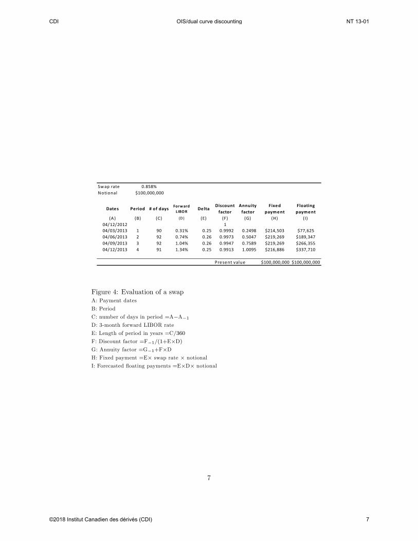
Under this classical approach, the rates used to compute the and at a given evaluation date 0 are the forward rates applicable over the period

[−1 ] observed at time 0. It is not surprising that in that case, the floatingleg of the swap agreement is worth par, because the discount rate is the same as

the rate earned over the payment period. Figure 4 illustrates the computations

to price the swap described in section 1.1.1.

1.3 Collateral posting

The above formula (4) can also be used to re-evaluate the swap at any interme-

diate date by using the forward rates observed at and setting = 1 and

=P

= ∆ Clearly, because the swap rate is fixed at initiation while the

reference forward rates are changing over time, the value of the swap agreement

does not stay constant at zero over its life time. If for instance at a given date

the value of the swap is positive, the fixed leg is worth more than the

6



Swap rate

Notional

Dates Period # of daysForward

LIBORDelta

Discount

factor

Annuity

factor

Fixed

payment

Floating

payment

(A) (B) (C) (D) (E) (F) (G) (H) (I)

04/12/2012 1

04/03/2013 1 90 0.31% 0.25 0.9992 0.2498 $214,503 $77,625

04/06/2013 2 92 0.74% 0.26 0.9973 0.5047 $219,269 $189,347

04/09/2013 3 92 1.04% 0.26 0.9947 0.7589 $219,269 $266,355

04/12/2013 4 91 1.34% 0.25 0.9913 1.0095 $216,886 $337,710

Present value $100,000,000 $100,000,000

$100,000,000

0.858%

Figure 4: Evaluation of a swap

A: Payment dates

B: Period

C: number of days in period =A−A−1D: 3-month forward LIBOR rate

E: Length of period in years =C360

F: Discount factor =F−1(1+E×D)G: Annuity factor =G−1+F×DH: Fixed payment =E× swap rate × notional

I: Forecasted floating payments =E×D× notional

7



floating leg at that time. If the fixed payer were to default on his payments,

then the fixed receiver would lose . For this reason, provisions in swap agree-

ments require that the fixed payer post the amount as collateral, so that, if

he defaults, the receiver can seize the collateral to cover his losses.

Collateral posting is governed by the CSA (Credit Support Annex) that

comes along with the swap agreement. Amounts posted as collateral earn inter-

est at the collateral rate, which is generally the Fed Fund effective rate, and are

adjusted periodically. Accordingly, assuming that the adjustment and payment

dates coincide, the net collateral payment of the fixed payer at date is

= − −1 (1 + ∆) = 1 − 1 = −−1 (1 + ∆)

2 Dual curve discounting

Dual curve discounting refers to the practice of using one interest rate curve

to project the swap cash flows and another curve to discount them. It is also

termed OIS discounting because Overnight Indexed Swap rates emerged from

the crisis as the correct risk-less investable rate which should be used for dis-

counting. The appellation “CSA discounting” is also often used to reflect the

Credit Support Annex that governs collateral posting in swap agreements, be-

cause the pricing methodology implied by the new paradigm takes this collateral

into consideration, while the classical approach completely ignores it. All three

designations refer to the same concept.

2.1 The pricing formula

Consider a basic fixed against floating swap as the one priced by the classical

methodology in Section (1.2). The discount rate in the pricing formula of dual

curve discounting is the collateral rate, that is, the forward compounded Fed

fund effective rates applicable between −1 and observed at date 0 These

forward rates can be recovered through OIS par swap rates. The formula also

takes as input basis swap spreads, as defined in Section (1.1.3), of OIS rate vs.

the reference rate. We denote by the basis swap spread, observed at date 0

of tenor periods. The process of dual curve discounting consists of constructing

the adjusted floating rate from the following equation:

e = − −1−1 − + −1∆

= 1 (6)

The floating payments are then projected using the adjusted e and all cashflows are discounted at the discount factors implied by the risk-less forward

curve. The net present value of the swap is still computed as the difference

between the present value of the fixed and floating fixed legs of the swap:

0 = −X=1

e∆

8



Swap rate

Notional

Date Period Days Forward

FedFund

Basis

spread

Delta Discount

factor

Annuity

factor

Floating

rate

Fixed

payment

Floating

payment

(A) (B) (C) (D) (E) (F) (G) (H) (I) (J) (K)

04/12/2012 1

04/03/2013 1 90 0.11% 20 0.25 0.9997 0.2499 0.31% $230,767 $77,500

04/06/2013 2 92 0.44% 25 0.26 0.9986 0.5051 0.74% $235,895 $188,847

04/09/2013 3 92 0.60% 32 0.26 0.9971 0.7599 1.06% $235,895 $270,574

04/12/2013 4 91 0.94% 40 0.25 0.9947 1.0114 1.58% $233,331 $399,841

Present value $100,404,551 $100,404,551

$100,000,000

0.923%

Figure 5: Evaluation of a swap using dual curve discounting

A: Payment dates

B: Period

C: number of days in period =A−A−1D: 3-month forward Fed-Fund rate

E: Basis spread corresponding to the number of periods F: Length of period in years =C360

G: Discount factor =G−1(1+F×D)H: Annuity factor =H−1+F×GI: Adjusted floating rate=(E×H-E−1×H−1-G+G−1)(F×G)J: Fixed payment =F× swap rate × notional

K: Forecasted floating payments =F×I× notional

and the par swap rate is given by1:

e∗ = P=1

e∆

(7)

Figure 5 illustrates the computations to price the swap described in section 1.1.1

using dual price discounting.

2.1.1 Explaining the adjusted forward floating rate eDual curve discounting essentially consists of constructing some adjusted for-

ward reference rate for the projection of the floating cash flows. In this section,

we give an interpretation of this adjustment.

First, assume that the basis swap spread is zero for all tenors . In this

case, it is easy to see that the adjusted forward rates are equal to the forward

1Notice that this formula uses market-quoted basis swap spreads to compute adjusted libor

rates and par swap rates. Formula (7) can also be used to compute adjusted libor rates and

basis swap spreads from market-quoted par swap rates.

9



risk-less rates. Indeed, in this case, equation (6) yields:

e∆ =− + −1

=−1− 1 = ∆

Hence, dual curve discounting reduces to the classical approach when the basis

swap spreads between the risk-less and the floating reference rates are zero.

Consider now the case where the basis swap spread is positive. Equation (6)

can be rewritten as:

e∆ =− + −1

+

− −1−1

= ∆ +

− −1

−1

(8)

which shows that the adjusted rate is nothing else than the forward risk-less rate

plus a spread. To fix ideas, assume that the floating reference rate is 3-month

LIBOR; Basis swap spreads indicate that 3-month LIBOR is exchanged against

3-month OIS rate over − 1 periods for −1 basis points paid at each period,and that 3-month LIBOR is also exchanged against 3-month OIS over periods

for basis points paid at each period. The spread in (8) indicates the value

of agreeing at date 0 to exchange the 3-Month LIBOR against the 3-month

OIS for one period between dates −1 and . It is simply the sum of the basis points paid each period up until period (properly compounded) minus

the sum of the −1 basis points paid each period up until period (properly

compounded). This can be interpreted as the forward LIBOR-OIS spread.

The forward LIBOR rate of section (1.2) and the adjusted forward LIBOR

rate e are both forward LIBOR rates. The first is computed using par fixed vsLIBOR swap rates, while the second is computed using forward OIS rates plus

the forward LIBOR-OIS rate spread. The difference between the two forward

rates amounts to the discount factors used to compute them from observed data:

the construction of the classical forward LIBOR rates uses discount factors

implied by LIBOR swap rates, while the construction of the adjusted forward

LIBOR uses discount factors implied by par OIS rates.

2.1.2 Some implications of dual curve discounting

As noted earlier, the forward curve used for discounting the cash flows is not that

of the floating rate (LIBOR or its equivalent), but rather that of the collateral

rate (generally the OIS rate). Moreover, the rates used to project the floating

payments are not equal to the “classical” forward floating rate. Now notice that

equation (6) defining the adjusted floating rate implies:

X=1

e∆ + = 1 + (9)

10



The left hand side of equation (9) is the present value of the floating leg of the

swap, where the floating payments are projected at the rate e and discountedwith the risk-less discount factor The right hand side of equation (9) is equal

to 1 if the basis swap spread for a tenor of periods is zero. The intuition

is that when the basis spread is zero, the classical approach is valid and the

floating leg must be worth par. On the other hand, if the basis swap spread is

positive, then the right hand side of equation (9) is greater than one. Therefore,

unlike in the classical approach, under dual curve discounting the floating leg

of the swap is worth more than par. This difference reflects the risk premium

embedded in the floating reference rate, which accounts for the liquidity and

default risk of the financial institutions participating in it.

Consider for instance OIS and fixed against LIBOR swaps. OIS bear negli-

gible risk because the notional of swaps is not actually exchanged and because

contractual parties have to post collateral. Receiving the LIBOR instead of the

OIS rate is a privilege since the former will always be greater, and the floating

leg of the LIBOR swap should be worth more than par. Before the 2007 crisis,

LIBOR-OIS spreads were close to zero. Even if it was known at that time that

the OIS rate was a better proxy for the risk- free rate, there was little need to

account for the risk premium because it did not make a significant difference.

During the crisis the spread blew up and practitioners were forced to switch

from the classical pricing method to dual curve discounting.

In the next section, we show that dual curve discounting is equivalent to

no-arbitrage pricing when financing costs are taken into consideration.

3 Dual curve discounting and no-arbitrage pric-

ing

No-arbitrage pricing dictates that two assets generating the same cash flows at

the same dates should have the same price. If this were not the case, arbitrageurs

would long the cheaper asset and short the other one, and immediately trade

away the difference in the two prices. Classical no-arbitrage pricing of a swap

consists of constructing a portfolio of traded swaps in such a way that the cash

flows of the fixed leg in the replicating portfolio equal those of the fixed leg of

the swap. By no-arbitrage arguments, the price of the fixed leg of the swap is

then the value of the replicating portfolio.

3.1 Conditions for classical no-arbitrage

Consider a replicating portfolio in the sense that its fixed payments match the

fixed payments of the swap. We index by and by the variables corresponding

to the swap and to the replicating portfolio respectively. Periods are indexed by

= 1 and dates are denoted by where 0 is the initial date. Accordingly,

for ∈ { } and = 0 denote by:

11



: notional

2 of instrument at date

: net present value of instrument at date

: present value of the fixed leg of instrument at date

∆ : length of period in years, ∆ =−−1360

: floating rate of instrument observed at date −1 and applicable during

period

: collateral rate3 observed at date date −1 and applicable during period

.

Consider an arbitrageur who is long the fixed leg of the swap and short the

fixed leg of the replicating portfolio. By construction, the fixed payments of the

swap and its replicating portfolio offset each other. The cash flow received by

the arbitrageur at date is then

− ¡ ∆−1 + (1 + ∆)

−1 −

+−1 −

¢+¡ ∆

−1 + (1 + ∆)×

−1 −

+

−1 −

¢ (10)

From the long side, the arbitrageur makes the floating payment ∆−1,

returns the previous period collateral plus interest (1 + ∆)−1 and takes the

new required collateral and finally makes a fictitious notional payment of

−1 −

so that the balance of the notional is The same logic applies

to the short side with the opposite sign.

Under the classical evaluation model, using the definition of the net present

value of instrument at date and the fact that the floating leg is worth par,

we have:

=

−

= (11)

Moreover, if the law of one price holds, we must have:

=

for all (12)

Substituting equations (11)-(12) into equation (10) yields:

−1 ( − )−

−1 ( −

) (13)

which is different from zero in general, unless

= = (14)

if we exclude the trivial case where the notional of the swap and its replicating

portfolio are equal.

Equation (14) says that for the no-arbitrage assumption to be valid, the

floating rates of the swap and of its replicating portfolio must be the same, and

must equal the collateral rate, otherwise the arbitrageur might have to inject

cash flow in order to maintain his positions. If the total cash flow injected

exceeded the initial difference in price between the replicating portfolio and the

2The notional is allowed to vary through time.3 may viewed as the par rate of an OIS initiated at date −1and ending at date

12



fixed leg, he would actually lose money at the closing of his positions. Assuming

that the replicating portfolio is constructed using swaps at the same floating rate

the total cash flow received by the arbitrageur is

( − )¡

−1 −

−1¢

A corollary of this no-arbitrage condition is that classical arbitrage pricing does

not work for LIBOR swaps since the LIBOR-OIS spread − is not zero.

Another corollary is that classical arbitrage pricing works for OIS swaps because

in that case the floating rate and the collateral rate are equal to the Fed fund

effective rate or its equivalent.

The intuition for the no-arbitrage condition for is the following. A long

position in the fixed leg of a swap has two financing costs: the notional finances

at the floating rate, while the net present value of the swap finances at the

collateral rate. It follows that there are two sources of financing distortion

between the replicating portfolio and the swap. First, the different swaps in the

replicating portfolio might not be defined on the same floating rate, and even

if it were the case, the floating rate of the replicating portfolio may be different

from the floating rate of the swap. Second, assuming that the floating rates are

all the same, they are generally different from the collateral rate (except for OIS

swaps). These distortions in financing costs show up in the interim cash flows

of the arbitrageur.

3.2 No-arbitrage pricing

The reason why fixed vs LIBOR swaps cannot be valued using classical no-

arbitrage pricing is that the construction of the replicating portfolio ignores

financing costs. Since in practice financing costs are not zero, the replication

process should take them into consideration. To use arbitrage pricing for a -

period LIBOR swap, we need to find a way so that the interim cash flows of

the arbitrageur given by equation (10) are zero. This can be achieved through

a basis swap that exchanges the collateral rate plus a fixed spread against the

LIBOR. Receiving a fixed rate against LIBOR over periods is equivalent

to receiving a fixed rate − against the collateral rate and receiving the

collateral plus the fixed spread against the LIBOR over the same periods.

Thus a long position on the fixed leg of a LIBOR swap is equivalent to a long

position on the fixed leg of an OIS swap and a short position on the basis swap.

The basis swap spread is determined in such a way that the basis swap is

worth par at date 0

It follows that the value of the period swap is the sum of the value of the

OIS swap and of the basis swap. Since the basis swap is worth par at date 0

the net present value of the period swap is equal to the net present value of

the OIS swap. The discounting is done at the forward collateral rate, which is

assumed to equal the forward risk-less rate:

0 = (− ) + − 1 (15)

13



where and are given by (1) and (2).

The no-arbitrage price given by equation (15) is the same as the dual curve

discounting price. Indeed equation (15) can be rewritten as

0 = ( + )− ( + 1) (16)

The first term in parentheses in the right hand side of equation (16) is the

present value of the fixed leg of the swap. The main idea behind dual curve

discounting is to compute an adjusted forward floating rate so that the second

term in the right hand side of equation (16) can be interpreted as the present

value of the floating leg. This can be readily verified by checking the second

formulation for the construction of the adjusted forward floating rate given by

equation (9).

4 Conclusion

A general presentation of dual curve discounting can be found in Tuckman

& Serrat (2012), Douglas and Decrem (2011a,b) and Kancharla (2012). We

conclude this brief presentation by reviewing some recent publications on dual

curve discounting in both academia and industry.

4.1 Practical issues

This subsection is inspired by an interview of David Kelly, director of the finan-

cial engineering department of Calypso, published in Risk magazine.

There are several challenges to the implementation of dual curve discounting

in practice. One of them is cross-currency curve construction.

1. There can be an option in the CSA that allows counterparties to post

collateral in different currencies. Pricing this option into the OIS curve is

a complex issue.

2. Calibration can be also difficult in the case of cross-currency swaps because

one has to calibrate an OIS curve in one currency based on the cross

currency basis.

3. Some swaps in one currency collateralize in another currency (this is the

case of Australian dollar swaps that collateralize in US dollar).

4. Another issue is that of the OIS curve segmentation; one may want for

instance to incorporate jumps in the short end of the curve, in order to

account for Central Bank meetings.

4.2 Selected recent developments in the industry

Dual curve discounting has created new markets for derivatives valuation and

risk management corporations.

14



SwapClear, the interest rate swap clearing service run by London-based LCH.

Clearnet, has begun shifting to OIS discounting in June 2010 and intended in

2011 to extend OIS discounting to its entire multiple currencies swap portfolio

(Sawyer 2011).

Principia Partners, a risk management software provider, launched a new

version of their platform that is able to support the shift in derivatives markets

towards OIS discounting (Worldwide Computer Products News, November 9,

2011).

Vancouver-based derivatives valuation and risk management software provider

Fincad recently added OIS curves to its platforms. Fincad builds OIS curves

for different currencies, including Japanese yen, pounds sterling, euro and Swiss

francs, and US dollar (Inside market Data, July 9, 2012).

KLP Asset Management, a subsidiary of a Norway-based insurance company

that manages NOK 227 billion in assets, replaced its interest rate derivatives

vendor by Quantify. The reason of this transaction is their need for a dual curve

discounting environment (Wireless news, November 6, 2012).

4.3 Selected recent contributions from the academia

A series of working papers have been published on the issue of dual curve

discounting in recent years. A first stream in this literature reports on em-

pirical evidence. Bianchetti and Carlicchi (2012) provide extensive evidence of

increased use of collateral, divergence between OIS and LIBOR, and explosion of

basis swap spreads. They also provide some empirical evidence that the market

abandoned the classical approach for the dual curve approach since March 2010.

Schwartz (2011) shows that liquidity risk is the predominant factor explaining

the LIBOR-OIS spread, ahead of credit risk.

Another group of researchers focus on developing a continuous-time model

for the adjusted forward rate. Mercurio (2010) proposes an extension of the

one-curve LIBOR Market Model (LMM) with stochastic volatility, where he

models the basis between OIS and FRA rates. He then shows that this model

is still flexible enough to result in closed-form prices for caps and swaptions.

The model is also able to handle simultaneous derivatives of different tenors.

Alvarez-Manilla (2012) proposes a non-martingale dynamics for the adjusted

forward rate. This contrasts with the works of Bianchetti (2010) and Mercurio

(2009) where the adjusted forward rate is a martingale.

No major paper on dual curve discounting has been published in the top-

rated financial journals, at least to our knowledge. One may wonder why there

is so little interest in academia about dual curve discounting. This lack of

interest may be due to the fact that, for researchers, there is little innovation

in using OIS rates as risk-less rate, and research is rather focused on the more

general problem of credit and liquidity risk. However, several technical issues

still remain to be addressed in practice.

15



References

[1] Alvarez-Manilla, M. (2012). Non-Martingale Dynamics for Two Curve

Derivatives Pricing. SSRN Working Paper Series, Rochester.

[2] Bianchetti, M. (2010). Two curves, one price. Risk magazine 23(8) : 66-72.

[3] Bianchetti, M. & M. Carlicchi (2012). Interest Rates After the Credit

Crunch: Multiple Curve Vanilla Derivatives and SABR. SSRN Working

Paper Series, Rochester.

[4] Douglas R. & P. Decrem (2011a). Interest rate Models: OIS & CSA dis-

counting, Learning Curve, Derivatives Week XX(26), July 4.

[5] Douglas R. & P. Decrem (2011b), OIS and CSA discounting, White paper,

Quantifi, May 13 2011. Downloaded from: http://fr.slideshare.net/.

[6] Inside Market Data (9 July 2012). Fincad Adds Overnight Index Swap

Curves to Valuation, Hedge Tools 27(40) : 9-9.

[7] Kancharla, S. (2012), OIS and Its Impact on Modeling, Calibration

and Funding of OTC Derivatives, Numerix LLC. Downloaded from

http://www.xenomorph.com/news/events/2012/wilmott/.

[8] Mercurio, F. (2009). Interest Rates and The Credit Crunch: New Formu-

las and Market Models. Bloomberg Portfolio Research Paper No. 2010-01-

FRONTIERS.

[9] Mercurio, F. (2010). A LIBOR Market Model with Stochastic Basis. SSRN

Working Paper Series, Rochester.

[10] Risk magazine (8 November 2012). OIS discounting for deriva-

tives, Interview of David Kelly. Source: http://www.risk.net/risk-

magazine/advertisement/2223295/sponsored-video-ois-discounting-for-

derivatives

[11] Sawyer, N. (2011). SwapClear may assist OIS development. FX Week,

22(36) : 1-2.

[12] Schwartz, K. (2011). Mind the Gap: Disentangling Credit and Liquidity in

Risk Spreads. SSRN Working Paper Series, Rochester.

[13] Tuckman, B. & A. Serrat (2012). Fixed income Securities: Tools for Today’s

Markets, 3rd Edition, John Wiley & Sons, Hoboken, New Jersey.

[14] Wireless News (November 6, 2012). Quantifi Integrates OIS Discounting

with KLP.

[15] Worldwide Computer Products News (November 9, 2011). Principia re-

leases Principia SFP version 6.6 with support for OIS discounting. (2011).

16



Documents

Note technique NT 13-01 - ICDcurve discounting, OIS discounting or CSA (Credit Support Annex) discounting. The variety of names given to it show that it can be understood from diﬀerent