Note on Panel Data Econometrics

Report by Sebastian Buhai∗

August, 2003

1 Introduction

Since longitudinal data sets contain observations over the same units(e.g. individuals, household, firms, industries, regions, countries) re-peated over a number of time periods, panel data techniques present ma-jor advantages over standard time-series or cross-sectional approaches,by combining their identifying features. The identification of time seriesparameters was usually based on notions of stationarity, predetermined-ness and uncorrelated shocks; identifying cross-sectional parameters tra-ditionally relied on exogenous instrumental variables and random sam-pling; working with panel data sets allows using all these resources andat the same time determines economists to think more about the natureand applicability of a particular technique to identify a parameter ofpotential interest.

Several improvements that working with panel data has over work-ing with conventional time-series or cross-sectional data are for instancementioned in Hsiao (2003). There is for instance a larger number of datapoints available, increasing therefore the degrees of freedom and reduc-ing the colinearity among explanatory variables. Next, panel data al-lows constructing and testing more complicated behavioral models thanpurely cross-sectional or time series data. Yet another plus is that wecan better study the dynamics of adjustment, such as for instance theeffect of unionism on economic behavior. A particular advantage of themicro-panel data sets is that they eliminate biases resulting from aggre-

∗Tinbergen Institute and Erasmus University Rotterdam; contact: Roetersstraat31, 1018 WB, Amsterdam; phone: 020-551 3561; fax: 020- 551 3555; email:buhai@tinbergen.nl

1

gation over micro-units; see Blundell (1988) for an interesting survey inthis sense or Blundell and Meghir (1990) for a more specific discussionon estimating life-cycle models. In a nutshell, the most acclaimed fea-tures of longitudinal sets are probably summarized in that they can oftenprovide the exogenous variation required to identify structural parame-ters through comparisons across periods covering policy changes and inthe possibility of following the same units over time, which facilitatesanalyzing dynamic responses and modelling unobserved heterogeneity.The main objective of this paper is to give a general overview of

the main trends and current status in panel data econometrics, build-ing on the guidelines given in Manuel Arellano’s lectures in the NAKEWorkshop from Rotterdam, June 10-13, 2003. Next to adopting a broad-spectrum approach, we will put some more emphasis on a few selectedthemes. We will insist for instance on the static longitudinal frameworkwith its basic motivations of controlling for unobserved heterogeneityand decomposing error structures, since much of this is recurrent inother sections. An extensive treatment of estimating covariance struc-tures for dynamic models, including the discussion of a concrete examplein Abowd and Card (1989), will also be provided. The overall structureof the paper is the following: section 2. will tackle static panel data mod-els; in section 3. the focus will be on time series models and dynamicerror components; section 4. will try to give the reader an impressionof dynamics with exogeneity versus predeterminedness; section 5. willbriefly discuss discrete choice models.

2 Static models

2.1 Unobserved heterogeneityThe rationale econometricians invoke when using panel data in generaland static regression models in the narrower sense, seems to be basedon two distinct motives: first, controlling for unobserved time-invariantheterogeneity in cross-sectional models and second, disentangling com-ponents of variance and studying the dynamics of cross-sectional pop-ulations. Loosely speaking, these reasons can be associated with thetwo main panel data techniques, the fixed effects and the random ef-fects models. In the remainder of this section we shall discuss issuespertaining to both these motivations.Consider the following cross-sectional regression model:

yi1 = βxi1 + ηi + vi1 (1)

Following the introductory discussion above we can approach the esti-mation of β in different ways, depending on our starting premise. If ηi is

2

observed then β can be immediately identified from a multiple regressionof y on x and η. If ηi is not observed however, in order to identify β weeither need lack of correlation between xi1 and ηi, so Cov(xi1, ηi) = 0,in which case we will estimate β as

β =Cov(xi1, yi1)

V ar(xi1)(2)

or we need to have an external instrument zi available so thatCov(zi, ηi) =0, Cov(zi,vi1) = 0 but Cov(zi, xi1) 6= 0, so that we can estimate

β =Cov(zi, yi1)

Cov(zi, xi1)(3)

When none of the approaches above is applicable we have a potentialproblem. Suppose however that we observe yi2 and xi2 for the sameindividuals in a second period:

yi2 = βxi2 + ηi + vi2 (4)

If we make the strict exogeneity assumption1 for the idiosyncraticdisturbance vit ,

E(vit|xi1, xi2, ηi) = 0, for t = 1, 2 (5)

then we can still identify β in a regression in first differences, albeit theindividual effect ηi is unobservable:

yi2 − yi1 = β(xi2 − xi1) + (vi2 − vi1) (6)

resulting in

β =Cov(∆xi2,∆yi2)

V ar(∆xi2)(7)

Arellano (2003) gives a few concrete examples where determiningthe coefficient of interest through first-differencing works and where thisdoes not work. For the first case we have the classical Cobb-Douglasproduction function, present among others also in Chamberlain (1984),

1The strict exogeneity assumption implies that explanatory variables in each timeperiod are uncorrelated with the idiosyncratic error in each time period, E(x

0isuit) =

0, ∀ s, t = 1, 2, ..T (with T = 2 in our case). In particular this assumption is muchstronger than the zero contemporaneous correlation E(x

0ituit) = 0, t = 1, 2, ..T . For

consistency of panel data estimation the E(x0isuit) = 0 condition suffices, allowing

for possible correlation between ci and vit for any t. Nonetheless standard forms ofstatistical inference rely on expression (5. See Wooldrige(2002) for a clear and indepth treatment of these issues.

3

where (1) represents a production function for an agricultural product.The following notations are imposed: i - farms, t - time periods (seasonsor years), yit - log output, xit - log of a variable input (e.g. labour), ηi - aninput remaining constant over time (e.g. soil quality), vit - a stochasticinput outside the farmer’s control (e.g. rainfall). We suppose that thesoil quality is known by the farmer but not by the researcher; henceif the farmers maximize expected profits there will be a cross-sectionalcorrelation between labour and soil quality, or, formally, between theregressor variable xit and the individual effect ηi. Suppose next that dataon yi2 and xi2 for a second period become available. Suppose also thatrainfall in the second period is independent of a farm’s labour demandin the two periods, thus checking for the exogeneity assumption abovehaving labour uncorrelated with rainfall at all lags and leads. Theneven in the absence of data on ηi, the availability of panel data affordsidentification of the technological parameter β.

While this was an example that worked, let us turn to one whichdoes not. This is the standard case of estimating the structural returnsto education. Consider again our regression equation in (1). We label byyit - log wage, xit - years of full time education, ηi - unobserved abilityand β - returns to education. The dilemma is that xit typically lackstime series variation. A regression in first differences will not identifyβ because in (7), V ar(∆xi2) would be virtually 0. So in this case paneldata analysis is not very useful; we would manage to solve this problemif we could get some exogenous instrumental variables such as data onsiblings for instance.

In the paragraphs above, talking about the unobserved heterogeneity,we have in fact introduced the fixed-effects models within panel data.Let us see more formally what are its basic assumptions. Take a randomsample (yi1, ..., yiT , xi1,..., xiT , ηi), i = 1, ...N and consider the modelfrom (1), which rewritten here for multiple t :

yit = x0itβ + ηi + vit (8)

The assumptions of this model are:A1.

E(vi|xi, ηi) = 0, for t = 1, ..., T (9)

where vi = (vi1, ..., viT )0 and xi = (xi1, ..., xiT )0.

A2.V ar(vi|xi, ηi) = σ2IT (10)

which means that the time-variant errors are conditionally homoskedas-tic and serially uncorrelated.

4

The fixed effects models are usually referred to as models where weallow for arbitrary correlation between the unobserved individual effectηi and the observed explanatory variable xit, contrasting with random ef-fects models where the permanent effect is independent of the regressors(Wooldridge (2002)). Assumption A1 above is the fundamental assump-tion since it puts forward the strict exogeneity condition. Panel datamodels without this assumption are more complex and shall be consid-ered later in this paper. The second assumption A2 is just an auxiliaryassumption needed for optimality of simple OLS estimators as it willbecome clearer below.

We shall now introduce the most popular estimator in panel dataanalysis, namely the within-group estimator (know also under severalother names, including covariance estimator, dummy-variable least squareestimator2 or fixed effects estimator). If we consider the equation in (8),estimating first differences works without problems if T = 2, when wecan apply OLS to the equation

∆yi2 = ∆x0i2β +∆vi2 (11)

When we have T ≥ 3 however, we could have some problems trying touse first differencing since this technique might induce serial correlation.Subsequent to first-differencing we will have a system of T −1 equationswhich can be written easier in the compact form

Dyi = DXiβ +Dvi (12)

with D being the (T − 1)× T matrix operator

D =

−1 1 0 . . . 0 00 −1 1 0 0. . .. . .. . .0 0 0 . . .−1 1

(13)

Provided E(Dvi|xi) = 0, we obtain unbiased and consistent estimatesfor β by OLS, for large N :

bβOLS =Ã

NXi=1

(DXi)0DXi

!−1 NXi=1

(DXi)0Dyi (14)

2See Verbeek(2000) for a brief discussion of the equivalence between the within-group and the dummy least square estimator.

5

If assumption A2 is however not respected we will face correlation be-tween the errors in the first differences and the x0s, so that

V ar(Dvi|xi) = σ2DD0 (15)

The optimal estimator in this case is the generalized least squares (GLS)estimator, which takes the form

bβWG =

ÃNXi=1

X 0iD

0(DD0)−1DXi

!−1 NXi=1

Xi0D0 (DD0)−1Dyi (16)

This is the within-group estimator and it is equivalent to its alternativeform as deviations from time means:

bβWG =

"NXi=1

TXt=1

(xit − xi)(xit − xi)0#−1 NX

i=1

TXt=1

(xit − xi)(yit − yi) (17)

The equivalence between (16) and (17) can be easiest seen if we label byQ the within-group operator

Q ≡ IT − u0/T = D0(DD0)−1D (18)

Q transforms the original time series into deviations from time means:eyi = Qyi, with elements are given by fyit = yit − yi. We obtain thusequation (17), an OLS in deviations from time means.

There is yet another alternative transformation of the original datathat results from first differencing and then applying GLS to the differ-enced data to remove the serial correlation induced in the first stage.This is the forward orthogonal deviations technique (see Arellano andBover (1995) for a detailed treatment). Consider the (T −1)×T matrix

A = (DD0)−1/2D (19)

so that A0A = Q defined above, and AA0 = IT−1. A T × 1 time serieserror transformed by A,

v∗i = Avit (20)

will consist of elements of the form

v∗it = ct[vit − 1

T − t(vi,t+1 + ...+ viT )] (21)

where c2t =T−t

T−t+1 .We eliminate individual effects by applying the orthogonal deviations

transformation without inducing serial correlation in the transformed

6

error as the case with first-differencing. The within-group estimator canthus be also regarded as OLS in orthogonal deviations.

So far we have been assuming that the auxiliary assumption A2(equation (10) above) was satisfied. The within-group estimator is op-timal under this assumption. The question is now how to estimate themodel when homoskedasticity and serial correlation are violated andwhen there would be thus inconsistent standard errors subsequent toestimation. There are two relevant cases to be considered. One is whenwe have panel data sets of fixed T and large N dimensions while thesecond situation is the treatment of the case for large T and fixed Ndimensions. For the second case there are not clear directions of per-forming the analysis, some variations being Newey-West estimators (seeArellano(2003) for a discussion). For the first case, if

V ar(v∗i |xi) = Ω(xi) (22)

where Ω(xi) is a symmetric matrix of order T , then the optimal estimatorcan be written as follows

bβUGLS =Ã

NXi=1

X∗0Ω−1(xi)X∗i

!−1 NXi=1

X∗0Ω−1(xi)y∗i (23)

Nevertheless this estimator is unfeasible (UGLS) because the matrix Ω isunknown. We would need to estimate this matrix using nonparametricmethods or similar techniques. The only case whereΩ could be estimatedin a straightforward manner is one where the conditional variance of v∗iin (22) is a constant but non-scalar matrix of the form

V ar(v∗i |xi) = Ω (24)

In this case the GLS estimator is feasible (FGLS) and has the followingform bβFGLS =

ÃNXi=1

X∗0bΩ−1X∗i

!−1 NXi=1

X∗0bΩ−1y∗i (25)

where bΩ = 1

N

NXi=1

bv∗i bv∗0i (26)

Since however most of the time we cannot ensure that we have (24),we have to think about intermediate possibilities. To this end we couldconsider a larger set of moments, as follows

E(xitv∗is) = 0, ∀s, t (27)

7

so as to use all past and future values to produce a GMM estimator. Ifthe auxiliary assumption A2 in (10) is not satisfied, then this estimatorwill be more efficient that the within-groups estimator, but less efficientthan the benchmark unfeasible estimator βUGLS in (23). Such an es-timator is obtained for example by using the π- matrix approach, alsoreferred to as the minimum-distance approach, of Chamberlain (1982,1984). We will however not cover this topic here, indicating Hsiao (2003)for a thorough review of this case.

2.2 Error componentsWe have been talking in the previous section about controlling for unob-served heterogeneity as one of the main reasons for working with paneldata. It is time we moved to the second motivation, namely separatingout permanent from transitory components of variation. Let us considera very basic variance-components model

yit = µ+ ηi + vit (28)

where µ - intercept, ηi ∼ iid(0, σ2η) and vit ∼ iid(0, σ2). ηi and vit areindependent of each other and

V ar(yit) = σ2η + σ2 (29)

Having (29) above, we see that σ2η/(σ2η + σ2) of the total variance is due

to the permanent time-invariant component.This model allows us to make a distinction between aggregate and in-

dividual transition probabilities. The individual transition probabilitiesgiven ηi are independent of the state of origin:

Pr(yit ∈ [a, b]|yi,t−1 ∈ [c, d], ηi) = Pr(yit ∈ [a, b]|ηi) (30)

Using (30), the aggregate probability will beZPr(yit ∈ [a, b]|ηi)dF (ηi|yi,t−1 ∈ [c, d]) (31)

We see thus that the decomposition in (28) allows us to distinguishbetween individual probability statements for units with given ηi andaggregate probabilities for groups of observationally equivalent units. Inorder to estimate this variance-components models we first try to esti-mate conditionally on ηi, in other words implementing an estimation ofthe realizations of permanent effects ηi that occur in the sample and thevariance σ2 (Arellano (2003)). The straightforward unbiased estimateswould then be bηi = yi − y, i = 1, ..., N (32)

8

and respectively

bσ2 = 1

N(T − 1)NXi=1

TXt=1

(yit − yi)2 (33)

The only problem is that we do not have yet an estimate of σ2η andtypically this is also of interest. The seemingly immediate way to getthis estimate would be the following. Having

V ar(yi) ≡ σ2 = σ2η +σ2

T(34)

an unbiased estimator of our statistics of interest can be obtained as

bσ2η = bσ2 − bσ2T (35)

The dilemma is that the estimator above can be negative by construc-tion. There will be thus cases where we won’t be able to estimate bσ2η.We also have to note that for large N and short T dimensions one canobtain precise estimates of σ2η and σ2 but not of ηi, while for small Nand large T sets we would be able to obtain good estimates of ηi and σ

2

but not of σ2η.

The regression version of the model discussed previously in (28) is

yit = µ(xit, fi) + ηi + vit (36)

whereµ(xit, fi) = x0itβ + f 0iν (37)

We allow for both time-invariant as well as time-varying conditioningvariables (fi, respectively xit). A very important assumption is thatboth error terms are uncorrelated with any of the regressors. This is incontrast with the unobserved heterogeneity discussion in the previoussubsection where the very rationale was to allow the unobserved indi-vidual effect ηi to be potentially correlated with the regressor. So herewe will have

E(ηi|xi1, ..., xiT , fi) = 0 (38)

and the varianceV ar(ηi|xi1, ..., xiT , fi) = σ2η (39)

Optimal estimation of the model is achieved using a specific GLSknown under the name Balestra-Nerlove estimator (Balestra and Nerlove(1966)). A short review of this technique as well as discussion on tests

9

for correlated unobserved heterogeneity can be found in Arellano (2003).

We move now to discuss an ever recurrent theme in the panel dataeconometrics literature, measurement error in variables. Start with thefollowing cross-sectional regression model

yi = α+ x†iβ + vi (40)

Suppose x†i is observed with an additive noise effect εi under the formxi:

xi = x†i + εi (41)

Further assume independence between all unobservables x†i , εi and vi.Then β is given by

β =Cov(yi, x

†i)

V ar(x†i)(42)

but x†i is unobservable. We try to get a better expression for β from

Cov(yi, xi)

V ar(xi)=

Cov(yi, x†i)

V ar(xi) + V ar(εi)=

β

1 + λ(43a)

with λ = V ar(εi)/V ar(x†i). If we assume that we have the means of as-

sessing the measurement error, so that we either know or we can estimateλ and σ2ε = V ar(εi) then from (43a) β can be determined :

β = (1 + λ)Cov(yi, xi)

V ar(xi)=

Cov(yi, xi)

V ar(xi)− σ2ε(44)

More generally however we need to find other ways to estimate β sincewe cannot always rely on approximating the size of the measurementerror. One solution would be to have a second noisy measure of x†i andto use this as an instrumental variable. Suppose

zi = x†i + ξi (45)

If ξi is independent of εi and other unobservables, zi can be successfullyused as an IV so that β is obtained as3

β =Cov(zi, yi)

Cov(zi, xi)(46)

3In fact we even have an overidentifying restriction in this problem since we canalso write

Cov(xi, yi)

Cov(xi, zi)= β

10

We have noticed that for linear regression problems the treatment ofmeasurement errors is possible; the problem becomes really difficultwhen we have a nonlinear regression framework where the measurementerror is no longer additively separable from the true value of the regres-sor. One good reference for further reading in this sector is Hausmanet al (1995). A detailed introduction to the literature on measurementerror in panel data is Baltagi (2001).We have not considered yet a model which combines unobserved het-

erogeneity and measurement error. Write the following linear regressionin a cross-section:

yi = x†iβ + ηi + vi (47)

having again a measurement error in x†i as in (41). All unobservables areindependent of each other, with the exception now that and ηi are notindependent. There will be in this case two bias components: the firstis due to the measurement error and it depends on σ2ε and the second isdue to the unobserved heterogeneity and it depends on the Cov(ηi, x

†i)

term4. Trying to bypass this problem by using first differences in apanel data series may exacerbate the error rather then eliminating it(see Arellano (2003) and the further references he gives). In principlethe problem arises when there is more time series dependence in x†ithan in εit. One important observations that follows is that findingsignificantly different results between regressions in first-differences andregressions in orthogonal deviations indicate a high chance that we havehave measurement error in the model.In general the availability of panel data helps to solve the problem

of measurement error bias by providing internal instruments but onlyas long as we can restrict the serial dependence of the measurementerror. Take a model with unobserved heterogeneity and a white noisemeasurement error, having T > 2. The moment conditions for the errorsin first-differences are

E

xi1...

xi,t−2xi,t+1...xiT

(∆yit −∆xitβ)

= 0, for t = 2, .., T (48)

This sort of moments and GMM estimators based on them have beenproposed before in the literature (see for instance Griliches and Hausman

4Sometimes these two biases tend to offset each other, for instance if β > 0and Cov(ηi, x

†i ) > 0, but a full offsetting only happens if Cov(ηi, x

†i ) = σ2εβ (Arel-

lano(2003)), something very unlikely to happen however.

11

(1986)). One thing to pay attention to is that if the latent variable x†i isalso white noise than the moment conditions above are still satisfied butfor any β, so the rank condition fails and we cannot identify the truevalue of the coefficient. The basic identification assumption is thereforethe time-series persistence in the x’s relative to the ε’s. These esti-mators are very useful in situations where first differencing aggravatesmeasurement error bias, as mentioned above.

3 Time series models for panel data

3.1 Covariance structures for error componentsThe time series models for panel data are motivated by a general inter-est in the time series properties of longitudinal data sets. Albeit we areinterested in separating transitory from permanent components of varia-tion as we saw before, or we want to test a theoretical model with specificpredictions and map this to the data (e.g. Hall and Mishkin (1982)), orwe like to use a predictive distribution in optimization problems underuncertainty (e.g. Chamberlain (2000)), we find all these issues tackledwithin the chapter of time series analysis in panel data sets.

One particular matter often arising in the panel data context is theheterogeneity in the individuals and the quest of distinguishing it frominherent individual dynamics in the data set. This problem is relevantespecially in short panels. Consider the following heterogeneous errorcomponents model

yit = ηi + vit (49)

where vit is white noise. As we saw in previous sections, for T = 2 wewill have

Cov(yi1, yi2) = σ2η (50)

sinceV ar(yi1) = V ar(yi2) = σ2η + σ2 (51)

Take now a homogeneous AR(1) model

yit = η + vit (52)

wherevit = αvi,t−1 + εit (53)

with η a constant, εit ∼ iid(0, σ2ε), vit ∼ iid(0, σ2) and σ2 = σ2ε/(1− α).For T = 2 we will get

V ar(yi1) = V ar(yi2) = σ2 (54)

12

and subsequentlyCov(yi1, yi2) = ασ2 (55)

The point is that there is no way to distinguish empirically betweenthe models in (49) and (52) when T = 2 and α ≥ 0. It is easy to seethis if we consider the observed autocorrelation ρ1. In the case of theheterogeneous model this is given by

ρ1 =σ2η/σ

2

1 + σ2η/σ2

(56)

while in the AR(1) modelρ1 = α (57)

So if for instance it happens that σ2η/σ2 = 4 and α = 0.8, then ρ1

will have the same value in both models (numerical example in Arel-lano (2003)). Following this argument, one can further check that aheterogeneous model of the type (49) with T = 3 this time will be indis-tinguishable from a homogeneous AR(2) model. This discussion can bealso carried out using moving average processes instead of autoregres-sive ones. These few examples suggest is that in order to carry out anonparametric test of heterogeneity we need to have large N and T andwe need to ensure the absence of structural breaks.One important feature in analyzing panel data is trying to distinguish

time effects; it might be for instance often useful to remove business cy-cles or seasonal effects, to control for trends or demographic characteris-tics and so on. Consider for discussion a model with individual-specifictrends used in the income modelling literature (e.g. Lillard and Weiss(1979), Hause (1980)):

yit = η0i + η1it+ vit (58)

This can be written in a vector notation as

yi = Sηi + vi (59)

with yi = (yi1, ..., yiT )0, ηi = (η0i, η1i)0, vi = (vi1, ..., viT )0 and S the T × 2

matrix

S =

1 11 2... ...1 T

(60)

If V ar(ηi) = Ωη and vit ∼ iid(0, σ2) and independent of ηi, the covari-ance matrix of yi is

Ω = SΩηS0 + σ2IT (61)

13

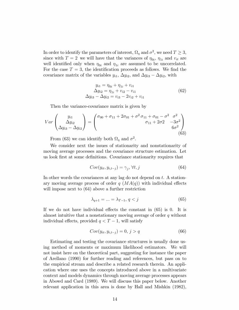
In order to identify the parameters of interest, Ωη and σ2, we need T ≥ 3,since with T = 2 we will have that the variances of η0i, η1i and vit arewell identified only when η0i and η1i are assumed to be uncorrelated.For the case T = 3, the identification proceeds as follows. We find thecovariance matrix of the variables yi1, ∆yi2, and ∆yi3 −∆yi2, with

yi1 = η0i + η1i + vi1∆yi2 = η1i + vi2 − vi1

∆yi3 −∆yi2 = vi3 − 2vi2 + vi1

(62)

Then the variance-covariance matrix is given by

V ar

yi1∆yi2

∆yi3 −∆yi2

=

σ00 + σ11 + 2σ01 + σ2 σ11 + σ01 − σ2 σ2

σ11 + 2σ2 −3σ26σ2

(63)

From (63) we can identify both Ωη and σ2.

We consider next the issues of stationarity and nonstationarity ofmoving average processes and the covariance structure estimation. Letus look first at some definitions. Covariance stationarity requires that

Cov(yit, yi,t−j) = γj, ∀t, j (64)

In other words the covariances at any lag do not depend on t. A station-ary moving average process of order q (MA(q)) with individual effectswill impose next to (64) above a further restriction

λq+1 = ... = λT−1, q < j (65)

If we do not have individual effects the constant in (65) is 0. It isalmost intuitive that a nonstationary moving average of order q withoutindividual effects, provided q < T − 1, will satisfy

Cov(yit, yi,t−j) = 0, j > q (66)

Estimating and testing the covariance structures is usually done us-ing method of moments or maximum likelihood estimators. We willnot insist here on the theoretical part, suggesting for instance the paperof Arellano (1990) for further reading and references, but pass on tothe empirical stream and describe a related research therein. An appli-cation where one uses the concepts introduced above in a multivariatecontext and models dynamics through moving average processes appearsin Abowd and Card (1989). We will discuss this paper below. Anotherrelevant application in this area is done by Hall and Mishkin (1982),

14

where predictions of the permanent income model are tested; a detailedreview of the econometrics in this latter paper is presented in Arellano(2003).Abowd and Card (1989) put forward an empirical analysis of individ-

ual earnings and hours data. Their paper summarizes the main featuresof the covariance structure of earnings and hours changes and comparesit with a structure implied by a simple version of the life-cycle laborsupply model. The authors use three different longitudinal surveys, twosamples from the Panel Study of Income Dynamics (PSID), a sample ofolder men from the National Longitudinal Survey of Men 49-59 (NLS)and a sample from the control group of the Seattle and Denver IncomeMaintenance Experiment (SIME/DIME). For each data set they findevidence that supports the restrictions implied by a nonstationary bi-variate MA(2) process without individual effects5. In order to controlfor differences in experience within and between the samples, the co-variances between the changes in logs of annual earnings and annualhours were computed using the residuals from multivariate regressionsof changes in earnings and hours on time dummies and potential experi-ence. A comparison of these results with previous literature dealing withcovariance structure of earnings such as Lillard and Weiss (1979), Hause(1980) or MaCurdy (1982), reveals some possible general results. Forinstance negative serial correlation between consecutive changes in logearnings seems to be a pervasive phenomenon, a bivariate MA(2) mov-ing average process seems to be adequate for describing the data (withan exception in Lillard and Weiss who find significant large higher-orderautocovariances of earnings) and nonstationarity appears to be the rule.The authors subsequently examine three statistical models that could

be considered the generators for the structure of earnings and hourschanges above. It is found that a relatively simple components-of-variance model explains the data from all three surveys. This con-structed model has three sources of earnings and hours variation:

∆yit =

µµ1

¶∆zit +∆uit + εit (67)

with ∆yit a vector of growth rates in earnings and hours of work, ∆zita shared component of earnings and hours variation ( a scalar MA(2)component) and ∆uit and εit bivariate white noise processes accountingfor the measurement error and respectively the permanent shocks.

5In other words, Abowd and Card (1989) obtain a representation wherecov[∆ log git,∆ log git−j ], cov[∆ log hit, ∆ log hit−j ] and cov[∆ log git, ∆ log hit−j ] areconstant for all t and are zero for |j| > 2, where g represents earnings and h representsworked hours.

15

As regards interpreting the predicted outcome, according to the life-cycle model the variation in the individual productivity affects earningsmore than hours. Abowd and Card’s (1989) empirical findings showhowever that on the contrary, the earnings and hours covary proportion-ally, which casts doubt on the labor supply interpretation of earningsand hours variation and puts forward the view that most changes inearnings and hours occur at fixed hourly wage rates.

3.2 Autoregressive models with individual effectsThe form of regression covariances within autoregressive structures aremore complex than those in moving average processes. If theMA processeslimit persistence to a given number of periods and imply linear momentrestrictions in the covariance matrix of the data, as we have seen inthe previous section, with autoregressive processes the situation is dif-ferent. They imply nonlinear covariance restrictions but provide at thesame time instrumental-variable conditions that are linear in the au-toregressive coefficients. Moreover the autoregressive model discussionusually centers around themes such as stationarity of initial conditions,homoskedasticity and unit roots, which were typical issues in time-seriesanalysis. Consider the following model

yit = λyi,t−1 + αi + εit, t = 0, 1..., T (68)

Let us assume that |λ| < 1. The within-group estimator of the regressionequation above is given then by

bλWG =

PNi=1

PTt=1(yit − yi)(yi,t−1 − yi,−1)PN

i=1

PTt=1(yi,t−1 − yi,−1)2

(69)

with yi = (1/T )PT

t=1 yit and yi,−1 = (1/T )PT

t=1 yi,t−1.It has been shown, using expressions (68) and (69) above (Nickell

(1981)) that the within-group estimator is inconsistent for fixed T andit is biased and inconsistent for large N and fixed T. This inconsistencyhas not been caused by any assumption about the individual effectsα, since they are eliminated anyway when estimating the within-groupregression. The problem is that the within transformed lagged error iscorrelated with the within transformed error. The bias disappears withT →∞, but it is very important for small values of T . Fortunately thereare ways to go around this inconsistency. Take first the first differencesin (68):

yit − yit−1 = λ(yi,t−1 − yi,t−1) + εit − εi,t−1, t = 2, ..., T (70)

16

Anderson and Hsiao (1981) proposed an instrumental variable estimatorfor λ, using yi,t−2 as an instrument for (70):

bλIV = PNi=1

PTt=1 yi,t−2(yit − yi,t−1)PN

i=1

PTt=1 yi,t−2(yi,t−1 − yi,t−2)

(71)

This estimator is consistent given that our assumption of no autocorre-lation of the idiosyncratic error term εit is met and provided that

p lim1

N(T − 1)NXi=1

TXt=2

(εit − εi,t−1)yi,t−2 = 0 (72)

Anderson and Hsiao also proposed an alternative instrument, yi,t−2 −yi,t−3, having a similar estimator expression and consistency conditionas in (71) and respectively (72), but having yi,t−2−yi,t−3 instead of the lagvalue yi,t−2. Of course this second estimator also requires an additionallag.

A method of moments approach can unify these estimators and elim-inate the disadvantages of the small sample sizes. It was thus suggestedthat the list of instruments is extended by exploiting additional momentconditions and letting their number vary with t. GMM estimators usingall available lags at each period as instruments for equations in first-differences were proposed by Holtz-Eakin et al (1988) and Arellano andBond (1991). This GMM estimator is represented as follows

bλGMM =£∆¡y0−1Z

¢V −1N (Z 0∆y−1)

¤−1 ¡∆y0−1Z

¢V −1N (Z 0∆y−1) (73)

where

Zi =

yi0 0 0 ... 0 ... 00 yi0 yi1 0 0... ... ...0 0 0 ... yi0 ... yi,T−2

(74)

According to standard GMM theory, an optimal choice of the inverseweighting matrix VN is one that gives the most efficient estimator, inother words the one that gives the smallest asymptotic covariance matrixfor bλGMM . Since the optimal weighting matrix is asymptotically propor-tional to the inverse of the covariance matrix of the sample moments(Verbeek (2000)), we have that the optimal matrix ought to satisfy

p limN→∞

VN = E(Z 0i∆εi∆ε0iZi)−1 (75)

In the standard case where we do not impose any restrictions on thecovariance matrix of εit we can obtain the optimal weighting matrix

17

using a first-step consistent estimator of λ and replacing the expectationin (75) by a sample average:

V optN = (

1

N

NXi=1

Z 0i∆bεi∆bε0iZi)−1 (76)

where ∆bεi is a residual vector obtained for instance by using VN = Ias a first-step consistent estimator. We have estimated here the optimalweighting matrix without imposing restrictions of homoskedascity; inparticular for the estimation we do not even need the non-autocorrelationassumption but this is needed for the validity of the moment conditions.

There is a whole literature on assumptions about the initial condi-tions, homoskedasticity and mean stationarity with subtopics such asestimation under stationarity, estimation under unrestricted initial con-ditions, estimation under heteroskedasticity, time effects in AR models,initial condition bias in short panels. Next to these, quite a number ofrelatively recent papers discuss problems of unit roots, cointegration andspurious regression within panel data. These latter problems are par-ticularly relevant in very long time-series dimension of the longitudinaldata sets (if T → ∞). These are all very important themes and muchcan be written on them, however we will not cover them in this generalreport. The interested reader is advised to consult Arellano (2003) andthe further references therein for an excellent treatment of the subjector Arellano and Honore (2001) for a shorter but concise overview.

4 Dynamic regression models

4.1 Models with exogenous regressors and unre-stricted serial correlation

Consider models of the type

yit = αyi,t−1 + x0itβ + ηi + vit (77)

where we assume that

E(vit|xi1, ..., xiT , ηi) = 0 (78)

Although this would seem exactly the autoregressive model analyzedin the previous section plus some exogenous variables, this is not thecase. While the autoregressive model was a time-series perspective ofmodelling the persistence in y0s, hence we assumed the v0s serially un-correlated, now we have an entirely different view. Lagged y is correlated

18

by construction with η and lagged v, but it might even be correlated withcontemporaneous v if v is serially correlated, which is not precluded by(78). Thus lagged y is in fact an endogenous explanatory variable in(77) with respect to both η and v.From assumption (78) we can work out, as in Arellano (2003),

E[xis(∆yit − α∆yi,t−1 −∆x0itβ)] = 0, ∀s, t (79)

We have therefore internal moment conditions that will ensure iden-tification of the model despite the unrestricted serial correlation and theendogeneity of y.Applications of this model arise in testing life-cycle models of con-

sumption of labor supply with habits. In such models the parameter ofinterest is the coefficient α of the lagged regressor, which measures theextent of habits. This parameter could not be identified in the absenceof exogenous IV’s since the effect of the genuine habits would be indis-tinguishable from the serial correlation in the unobservable. One citedexample in this stream of literature is Becker et al (1994). They considera model for cigarette consumption using US panel data:

cit = θci,t−1 + βθci,t+1 + γpit + ηi + δt + vit (80)

where cit - annual per capita cigarette consumption by state, in packsand pit - average cigarette price per pack; β - discount factor. Beckeret al are interested in investigating whether smoking is addictive byconsidering the response of cigarette consumption to a change in prices.

The idiosyncratic errors capture unobserved life-cycle utility shifters,likely to be serially correlated. Thus even in the absence of addiction(θ = 0), we would still expect cit to be autocorrelated, and in particularto find a non-zero effect of ci,t−1 in (80). The identification strategyrelies thus on identifying θ, β and γ from the assumption that prices arestrictly exogenous relative to the unobserved utility shift variables.

4.2 Models with predetermined variablesThe models in this section have idiosyncratic errors that are uncorre-lated with current and lagged values of the conditioning variables, butmight be correlated with their future values, being "predetermined" inthis sense. The conditioning variables can be explanatory variables inthe equation or lagged values of these variables, but also external instru-ments.The moment conditions satisfied by the errors in the models with

predetermined variables are sequential moment conditions of the type

E(vit|zi1, ..., zit) = 0 (81)

19

Take for illustration the partial adjustment model in (77) in the preced-ing subsection and formulate its sequential moment condition require-ment:

E(vit|yi,t−1,xit,ηi) = 0 (82)

It is interesting to seek the differences between this assumption aboveand the corresponding assumption in the strictly exogenous model inthe previous subsection, namely expression (78). Arellano and Honore(2001) tell us that there are two main differences. In the first place(82) implies lack of autocorrelation in vit whereas the previous modelallowed for unrestricted serial correlation. Secondly, the assumption inthe strictly exogenous variables model from (78) implies that forecastsof xit given xi,t−1, yi,t−1 and additive effects are not affected by yi,t−1.In terms of identification, let us take the example of T = 3 in Arel-

lano and Honore (2001) where we had the following equation in firstdifferences

y3 − y2 = α(y2 − y1) + β0(x3 − x2) + β1(x2 − x1) + (v3 − v2) (83)

Using the exogenous variable model assumption, the parameters α, β0and β1 are potentially identifiable just from the moment conditions

E(xis∆vi3) = 0, s = 1, 2, 3 (84)

Conversely, in the predetermined variables model, the moment condi-tions that potentially identify α, β0 and β1 areE(yi1∆vi3) = 0

E(xi1∆vi3) = 0E(xi2∆vi3) = 0

(85)

The problem is that the two models have only two moment conditions incommon which are not however sufficient to identify the three parameters(Arellano (2003)).

5 Discrete choice models

The discrete or limited dependent variables combined with panel dataoften complicates considerably the estimation. This happens becausein longitudinal data sets often the different observations on the sameunit are not independent which leads to correlation between different er-ror terms and subsequently complicates the likelihood functions of suchmodels. One good overview of the literature in this specific fields is Mad-dala (1987), while for an up-to-date presentation of the current statusof research in the area the reader can consult Arellano (2001).

20

Consider for illustration a binary choice model:

y∗it = x0itβ + αi + εit (86)

where we observe yit = 1 if y∗it > 0 and yit = 0 otherwise. We can treatα as a fixed unknown parameter which means that the log likelihoodfunction is given by

logL=Xi,t

yit logF (αi + x0itβ)

+Xi,t

(1− yit) log[1− F (αi + x0itβ)] (87)

Maximizing this function with respect to β and αi results in con-sistent estimators only provided that T → ∞. This is known as theincidental parameters problem.

Fortunately for linear models β can be identified using the within-group estimator as long as T ≥ 2. The consistent estimator for β isgiven by the solution bβ to the equation (Arellano (2001)):

1

TN

NXi=1

TXt=1

(xit − xi)[(yit − yi)− (xit − xi)0bβ] = 0 (88)

However this does not solve our problem for nonlinear models and thuswe need to think of a way to maximize the likelihood. One idea is to finda sufficient statistic for αi so that the distribution of the data given thisstatistic does not depend on αi, and to use the likelihood conditionalon it so as to make inferences about β. This has been implementedfirst in Andersen (1970) and it is known under the name of conditionalmaximum likelihood estimator.

For the linear model with normal errors the sufficient statistic for α isthe mean yi. It is easy to show that for these linear setting, maximizingthe conditional maximum likelihood by using this statistic is equivalentwith using the within-group estimator for β. However the result cannotbe generalized to nonlinear models since it has been shown for instancethat no statistic of the type required here exists for the probit model,reason why a fixed effects probit model cannot consistently be estimatedfor fixed T (see Verbeek (2000) for a review).

In the random effects setting we assume lack of correlation in theidiosyncratic error term

uit ≡ ai + εit (89)

21

which implies that one can write the joint probability as

f(yi1, ..., yiT |xi1, ..., xiT , β) =Z ∞

−∞

"Yt

f(yit|xit, αi, β)

#f(αi)dαi (90)

which requires in principle numerical integration over one dimension.However this is extremely difficult and hence the most common practiceis to start with an assumption of multivariate normal distribution ofui1,...,uiT (see Maddala (1987) for a more in depth discussion). Thisbrings us to the random effects probit model. In practice using standardprobit maximum likelihood is consistent, but inefficient. The results canbe used however in an iterative maximum likelihood procedure based onthe expression in (90).

There is a fast growing literature on discrete choice models withpanel data. It is not our purpose to cover here for instance maximumscore estimation (see Manski (1987)) or maximizing alternative types oflikelihood functions As also mentioned above, a good survey of recentresearch in the field is contained in Arellano (2001).

ReferencesAbowd, J.M. and D. Card (1989), "On the Covariance Structure of

Earnings and Hours Changes", Econometrica, 57, 411-445

Andersen, E., B. (1970), "Asymptotic Properties of Conditional Max-imum Likelihood Estimation", Journal of the Royal Statistical Society,Series B, 32, 283-301

Anderson, T. and C. Hsiao (1981), "Estimation of Dynamic Modelswith Error Components", Journal of the American Statistical Associa-tion, 76, 598-606

Arellano, M. (1990), "Testing for Autocorrelation in Dynamic Ran-dom Effects Models", Review of Economic Studies, 57, 127-134

Arellano, M. (2001), "Discrete Choices with Panel Data", CEMFI,Working Paper 0101

Arellano, M. (2003), Panel Data Econometrics, Oxford UniversityPress: Advanced Texts in Econometrics

Arellano, M. and S.R. Bond (1991), "Some Tests of Specifications forPanel Data: Monte Carlo Evidence and an Application to EmploymentEquations", Review of Economic Studies, 58, 277-297

Arellano, M. andO. Bover (1995), "Another Look at the Instrumental-Variable Estimation of Error-Components Models", Journal of Econo-metrics, 68, 29-51

22

Arellano, M. and B. Honore (2001), ”Panel Data Models: Some Re-cent Developments”, in J.J. Heckman and E. Leamer (eds.): Handbookof Econometrics, vol 5, ch. 53, North-HollandBalestra, P. and M. Nerlove (1966), " Pooling Cross Section and

Time Series Data in the Estimation of a Dynamic Model: The Demandfor Natural Gas", Econometrica, 34, 585-612Baltagi, B. H. (2001), Econometric Analysis of Panel Data, Wiley,

2nd editionBecker, G., M. Grossman and K. Murphy (1994), " An Empirical

Analysis of Cigarette Addiction", American Economic Review, 84, 396-418Blundell, R. (1988), "Consumer behavior: Theory and Empirical

Evidence- A Survey", The Economic Journal 98, 16-65

Blundell, R. and C. Meghir (1990), "Panel Data and Life-Cycle Mod-els", in J. Hartog, G. Ridder and J. Theeuwes (eds.): Panel Data andLabor Market Studies, North-Holland, Amsterdam, 231-252Chamberlain, G. (1982), "Multivariate Regression Models for Panel

Data", Journal of Econometrics, 18, 5-46Chamberlain, G. (1984), "Panel Data", in Z. Griliches and M.D.

Intriligator (eds.): Handbook of Econometrics, vol. 2, ch. 22, North-HollandChamberlain, G. (2000), "Econometrics and Decision Theory", Jour-

nal of Econometrics, 95, 255-283Griliches, Z. and J.A. Hausman (1986), "Errors in Variables in Panel

Data", Journal of Econometrics, 31, 93-118Hall, R. and F. Mishkin (1982), "The Sensitivity of Consumption to

Transitory Income: Estimates from Panel Data on Households", Econo-metrica, 50, 461-481Hause, J.C. (1980), "The Fine Structure of Earnings and On-The-Job

Training Hypothesis", Econometrica, 48, No. 4, 1013-29Hausman, J.A., W.K. Newey, and J.L. Powell (1995), "Nonlinear Er-

rors in Variables Estimation of Some Engel Curves", Journal of Econo-metrics, 65, 205-233Holtz-Eakin, D., W. Newey and H. Rosen (1988), "Estimating Vector

Autoregressions with Panel Data", Econometrica, 56, 1371-1395Hsiao, C. (2003), Analysis of Panel Data, Cambridge University

Press, 2nd EditionLillard, L. and Y. Weiss (1979), "Components of Variation in Panel

Earnings Data: American Scientists 1960-1970", Econometrica, 47, 437-454

23

MaCurdy, T. E. (1982), "The Use of Time-Series Processes to Modelthe Error Structure of Earnings in a Longitudinal Data Analysis", Jour-nal of Econometrics, 18, 83-114

Maddala, G.S. (1987), "Limited Dependent Variable Models UsingPanel Data", The Journal of Human Resources, 22, 307-338

Manski, C. (1987), "Semiparametric Analysis of Random Effects Lin-ear Models from Binary Panel Data", Econometrica, 55, 357-362

Nickell, S. (1981), "Biases in Dynamic Models with Fixed Effects",Econometrica, 49, 1417-1426

Verbeek, M. (2000), A guide to Modern Econometrics, Wiley

Wooldridge, J. M. (2002), Econometric Analysis of Cross-Section andPanel Data, MIT

24