Embed Size (px)
Citation preview
1
NORTH PACIFIC RESEARCH BOARD
BERING SEA INTEGRATED ECOSYSTEM RESEARCH PROGRAM
FINAL REPORT
Ichthyoplankton: horizontal, vertical, and temporal distribution of larvae and juveniles of Walleye
Pollock, Pacific Cod, and Arrowtooth Flounder, and transport pathways between nursery areas
NPRB BSIERP Project B53 Final Report
Janet Duffy-Anderson1, Franz Mueter
2, Nicola Hillgruber
2, Ann Matarese
1, Jeffrey Napp
1, Lisa Eisner
3, T.
Smart4, 5
, Elizabeth Siddon2, 1
, Lisa De Forest1, Colleen Petrik
2, 6
1Alaska Fisheries Science Center, National Oceanic and Atmospheric Administration, 7600 Sand Point
Way NE, Seattle, WA 98115, USA
2University of Alaska Fairbanks, School of Fisheries and Ocean Sciences, 17101 Point Lena Loop Road,
Juneau, AK 99801 USA
3Ted Stevens Marine Research Institute, Alaska Fisheries Science Center, National Marine Fisheries
Service, National Oceanic and Atmospheric Administration, 17109 Pt. Lena Loop Road, Juneau, AK
99801, USA
4School of Aquatic and Fishery Sciences, University of Washington, Seattle, WA 98195-5020, USA
5Present affiliation: Marine Resources Research Institute, South Carolina Department of Natural
Resources, Charleston, South Carolina 29422, USA
6Present affiliation: UC Santa Cruz, Institute of Marine Sciences, 110 Shaffer Rd., Santa Cruz, CA 95060,
USA
December 2014
2
Table of Contents
Page
Abstract ........................................................................................................................................................... 3
Study Chronology ........................................................................................................................................... 6
General Introduction ....................................................................................................................................... 8
BSIERP Hypotheses ....................................................................................................................................... 11
Project Objectives ........................................................................................................................................... 12
Chapter 1 ......................................................................................................................................................... 14
Chapter 2 ......................................................................................................................................................... 52
Chapter 3 ......................................................................................................................................................... 88
Chapter 4 ......................................................................................................................................................... 115
Chapter 5 ......................................................................................................................................................... 148
Chapter 6 ......................................................................................................................................................... 189
Chapter 7 ......................................................................................................................................................... 213
Overall Conclusions ........................................................................................................................................ 267
BSIERP and Bering Sea Project Connections ................................................................................................ 270
Management Implications ............................................................................................................................... 272
Publications ..................................................................................................................................................... 273
Poster and Oral Presentations ......................................................................................................................... 275
Outreach .......................................................................................................................................................... 278
Acknowlegements ........................................................................................................................................... 280
3
Abstract
This project component (B53) of the Bering Sea Integrated Ecosystem Research Program (BSIERP), a
six-year multidisciplinary research effort sponsored by the North Pacific Research Board to study the
Bering Sea ecosystem, was designed to examine linkages between physical oceanographic variables,
biotic modulators, and distribution and abundance of three target fish species in the eastern Bering Sea
(EBS): Walleye Pollock (Gadus chalcogrammus, previously described as Theragra chalcogramma),
Pacific Cod (Gadus macrocephalus), and Arrowtooth Flounder (Atheresthes stomias). Effort focused
primarily on Walleye Pollock due to limited data availability on Pacific Cod and Arrowtooth Flounder.
Studies were based on historical zooplankton, ichthyoplankton, and physical data (1985-2010) collected
by the NOAA/Alaska Fisheries Science Center over the Bering Sea shelf as well as on a series of
seasonal, collaborative cruises that occurred 2008-2010 which were part of the BSIERP. Data derived
from the above investigations were applied to a biophysical model developed to examine interannual
patterns in Walleye Pollock distribution and abundance. The model work was funded, in part, with
monies from project B53 and with funds provided through the Bering Ecosystem STudy (BEST)
Synthesis Program, a Bering Sea research synthesis program sponsored by the National Science
Foundation. Cumulative results of this work provide a better understanding of the potential effects of
hydrographic variations in rearing conditions, transport, dispersal, and distribution of early life stages of
Walleye Pollock in the eastern Bering Sea.
In the first part of the project we examined factors affecting distribution, abundance and
community composition of larval fish assemblages, which included all three target species, over the
Bering Sea shelf and determined: 1) A strong cross-shelf gradient delineates slope and shelf assemblages
which is influenced by water masses emanating from the Gulf of Alaska, 2) Larval species assemblages in
the Bering Sea differ between warm and cold periods, with larval abundances (including Walleye
Pollock) being generally greater in warm years, and 3) Community-level patterns in larval fish
composition reflect species-specific responses to climate change.
The next part of the project involved a comprehensive suite of studies designed to examine
factors influencing distribution and abundance of young Walleye Pollock over the Bering Sea shelf.
First, abiotic and biotic variables were examined for effects on distribution and abundance of
Walleye Pollock larval stages. From this project it was found that: 1) The influence of temperature on
abundances of larval and juvenile Walleye Pollock increases with fish ontogeny, 2) Winds enhance the
transport of early life stages from initial spawning locations to shallower depths over the continental shelf,
3) Localized measurements of zooplankton prey are a better indicator of young pollock abundance than
4
broad-scale measurements that are integrated over the shelf, and 4) Temperature is a major driving force
structuring variability in abundance of Walleye Pollock in their first year of life.
Second, the effects of temperature on young Walleye Pollock were examined in greater detail in a
study designed to determine whether early life stages undergo spatial shifts in response to changing
temperature conditions, and test whether temperature affects the phenology of developmental events. It
was found that: 1) Walleye Pollock early life stages are distributed further east over the continental shelf
in warm years compared to cold years, and 2) Differences in the timing of density peaks support the
hypothesis that the timing of spawning, hatching, larval development, and juvenile transition are
temperature-dependent.
Third, a study of the factors affecting vertical distributions was undertaken. Results from this
investigation found: 1) Walleye Pollock demonstrate a decrease in the depth of occurrence following
hatching, indicating an ontogenetic change in vertical distribution, 2) Walleye Pollock vertical
distributions are related to the date of collection, water column depth, and thermocline depth, 3) Non-
feeding stages (eggs and yolksac larvae) do not exhibit diel vertical migration, 4) Flexion and postflexion
stage larvae, 10.0–24.5 mm SL undergo regular diel migrations (0–20 m, night; 10–40 m, day), 5)
Vertical distributions and diel migration a trade-off between prey access and predation risk for postflexion
larvae, and 6) Vertical distributions of Walleye Pollock eggs, yolksac larvae, and preflexion larvae in the
Bering Sea are different from previously-documented distributions in other ecosystems.
Fourth, we sought to determine mechanisms driving the observed spatial shifts in distribution of
young Walleye Pollock in warm and cold years. To accomplish this we developed a biophysical model of
spawning and dispersal, utilizing the data derived from the above investigations as input data, to examine
spawning, drift and connectivity of Walleye Pollock populations over the Bering Sea shelf in warm and
cold years. Model results indicate that: 1) Neither interannual variations in advection nor advances or
delays in spawning time adequately represent the field-observed differences in distribution between
warm and cold years, 2) Changes to spawning areas, particularly spatial contractions of spawning areas in
cold years, resulted in modeled distributions that were most similar to observations, and 3) The location
of spawning Walleye Pollock in reference to cross-shelf circulation patterns is important in determining
the distribution of eggs and larvae.
Another part of the project sought to resolve taxonomy of Arrowtooth (Atheresthes stomias) and
Kamchatka (Atheresthes evermanni) Flounder larvae in the eastern Bering Sea. Results show that: 1)
Arrowtooth Flounder and Kamchatka Flounder can be successfully identified to the species level through
molecular approaches, and 2) Arrowtooth Flounder 6.0–12.0 mm SL and ≥ 18.0 mm SL can be identified
to the species level using morphological techniques alone, but species identification of individuals 12.1–
5
17.9 mm SL remains confounded by morphological similarities between the two species. Results indicate
that molecular approaches must be used to conclusively identify Arrowtooth Flounder from Kamchatka
Flounder in the 12.1 – 17.9 mm SL size range. Work on the ecology of larvae of the two flounder species
suggests that: 1) the distribution of larvae (< 25.0 mm SL) of both Arrowtooth Flounder and Kamchatka
Flounder is similar in the eastern Bering Sea; however, juvenile (≥ 25.0 mm SL) Kamchatka Flounder
occur closer to the shelf break and in deeper water than juvenile Arrowtooth Flounder, and 2) Kamchatka
Flounder larvae and Arrowtooth Flounder larvae have similar lipid content in the larval and juvenile
stages when corrected for length. Results show that Kamchatka Flounder and Arrowtooth Flounder
spatially co-occur over the Bering Sea slope and shelf, but Arrowtooth Flounder appears to have a wider
distribution over the shelf than Kamchatka Flounder.
Taken collectively, our results indicate that abundance and distribution of fish larvae in the Bering Sea are
influenced by abiotic factors such as temperature, oceanographic currents, light levels, water column
stratification, seascape topography, water depth, and winds, as well as by biotic variables including prey
availability, initial spawning location, and timing of spawning. Moreover, we found there is ecological
plasticity in the responses of young fish to these various forcing factors depending on overall ecosystem
state (warm vs. cold conditions).
Keywords: Walleye Pollock, Bering Sea, larvae, ichthyoplankton, distribution, abundance, Arrowtooth
Flounder, Pacific Cod, survey, model
Citation: Duffy-Anderson, J.T., Mueter, F.J., Hillgruber, N., Matarese, A., Napp, J., Eisner, L., Smart, T.,
Siddon, E., De Forest, L., Petrik, C. 2014. Horizontal, vertical, and temporal distribution of larvae and
juveniles of Walleye Pollock, and transport pathways between nursery areas. NPRB BSIERP Project B53
Final Report, 274 p.
6
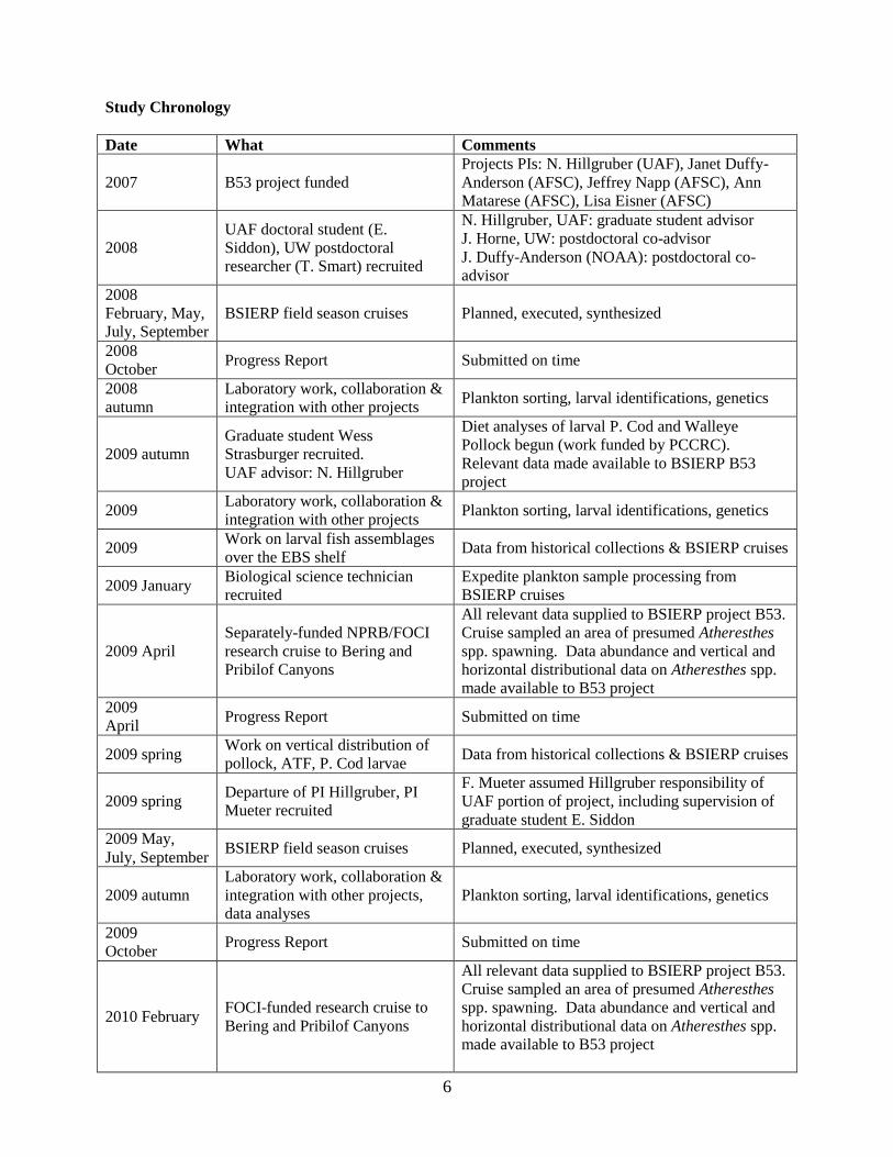
Study Chronology
Date What Comments
2007 B53 project funded
Projects PIs: N. Hillgruber (UAF), Janet Duffy-
Anderson (AFSC), Jeffrey Napp (AFSC), Ann
Matarese (AFSC), Lisa Eisner (AFSC)
2008
UAF doctoral student (E.
Siddon), UW postdoctoral
researcher (T. Smart) recruited
N. Hillgruber, UAF: graduate student advisor
J. Horne, UW: postdoctoral co-advisor
J. Duffy-Anderson (NOAA): postdoctoral co-
advisor
2008
February, May,
July, September
BSIERP field season cruises Planned, executed, synthesized
2008
October Progress Report Submitted on time
2008
autumn
Laboratory work, collaboration &
integration with other projects Plankton sorting, larval identifications, genetics
2009 autumn
Graduate student Wess
Strasburger recruited.
UAF advisor: N. Hillgruber
Diet analyses of larval P. Cod and Walleye
Pollock begun (work funded by PCCRC).
Relevant data made available to BSIERP B53
project
2009 Laboratory work, collaboration &
integration with other projects Plankton sorting, larval identifications, genetics
2009 Work on larval fish assemblages
over the EBS shelf Data from historical collections & BSIERP cruises
2009 January Biological science technician
recruited
Expedite plankton sample processing from
BSIERP cruises
2009 April
Separately-funded NPRB/FOCI
research cruise to Bering and
Pribilof Canyons
All relevant data supplied to BSIERP project B53.
Cruise sampled an area of presumed Atheresthes
spp. spawning. Data abundance and vertical and
horizontal distributional data on Atheresthes spp.
made available to B53 project
2009
April Progress Report Submitted on time
2009 spring Work on vertical distribution of
pollock, ATF, P. Cod larvae Data from historical collections & BSIERP cruises
2009 spring Departure of PI Hillgruber, PI
Mueter recruited
F. Mueter assumed Hillgruber responsibility of
UAF portion of project, including supervision of
graduate student E. Siddon
2009 May,
July, September BSIERP field season cruises Planned, executed, synthesized
2009 autumn
Laboratory work, collaboration &
integration with other projects,
data analyses
Plankton sorting, larval identifications, genetics
2009
October Progress Report Submitted on time
2010 February FOCI-funded research cruise to
Bering and Pribilof Canyons
All relevant data supplied to BSIERP project B53.
Cruise sampled an area of presumed Atheresthes
spp. spawning. Data abundance and vertical and
horizontal distributional data on Atheresthes spp.
made available to B53 project
7
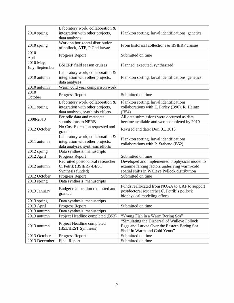
2010 spring
Laboratory work, collaboration &
integration with other projects,
data analyses
Plankton sorting, larval identifications, genetics
2010 spring Work on horizontal distribution
of pollock, ATF, P Cod larvae From historical collections & BSIERP cruises
2010
April Progress Report Submitted on time
2010 May,
July, September BSIERP field season cruises Planned, executed, synthesized
2010 autumn
Laboratory work, collaboration &
integration with other projects,
data analyses
Plankton sorting, larval identifications, genetics
2010 autumn Warm cold year comparison work
2010
October Progress Report Submitted on time
2011 spring
Laboratory work, collaboration &
integration with other projects,
data analyses, synthesis efforts
Plankton sorting, larval identifications,
collaborations with E. Farley (B90), R. Heintz
(B54)
2008-2010 Periodic data and metadata
submissions to NPRB
All data submissions were occurred as data
became available and were completed by 2010
2012 October No Cost Extension requested and
granted Revised end date: Dec. 31, 2013
2011 autumn
Laboratory work, collaboration &
integration with other projects,
data analyses, synthesis efforts
Plankton sorting, larval identifications,
collaborations with P. Stabeno (B52)
2012 spring Data synthesis, manuscripts
2012 April Progress Report Submitted on time
2012 autumn
Recruited postdoctoral researcher
C. Petrik (BSIERP-BEST
Synthesis funded)
Developed and implemented biophysical model to
examine farcing factors underlying warm-cold
spatial shifts in Walleye Pollock distribution
2012 October Progress Report Submitted on time
2013 spring Data synthesis, manuscripts
2013 January Budget reallocation requested and
granted
Funds reallocated from NOAA to UAF to support
postdoctoral researcher C. Petrik’s pollock
biophysical modeling efforts
2013 spring Data synthesis, manuscripts
2013 April Progress Report Submitted on time
2013 autumn Data synthesis, manuscripts
2013 autumn Project Headline completed (B53) “Young Fish in a Warm Bering Sea”
2013 autumn Project Headline completed
(B53/BEST Synthesis)
“Simulating the Dispersal of Walleye Pollock
Eggs and Larvae Over the Eastern Bering Sea
Shelf in Warm and Cold Years” 2013 October Progress Report Submitted on time
2013 December Final Report Submitted on time
8
General Introduction
Walleye Pollock (Gadus chalcogrammus, also described as Theragra chalcogramma) are sub-
Arctic gadids found from Japan to the Chukchi Sea to central California. Walleye Pollock (also refered to
as pollock, herein) are a semi-pelagic species that supports a major fishery in the rich waters of the Pacific
subarctic, where catches have ranged from approximately 0.7 – 1.7 million metric tons in the Eastern
Bering Sea (EBS) and Gulf of Alaska (GOA) since 1984. Ex-vessel value for these catches is
approximately 400 million US dollars per year in the last decade. Fishery targets include roe in the winter
and fillets throughout the spring and summer. Not only are pollock of significant commercial interest,
they are also a central component of the food web in the eastern Bering Sea, serving as prey for fish,
marine mammals, and seabirds.
Walleye Pollock population fluctuation has been linked to broad-scale climate variability
including oscillating phases of the Pacific Decadal Oscillation and the Aleutian Low. Hunt et al. (2002)
drew on these observed relationships to develop the Oscillating Control Hypothesis (OCH), a conceptual
theory predicting ecosystem responses to climate phase shifts. Specifically, the hypothesis predicted that
warm climate conditions would promote an early ice retreat, stratifying waters and maintaining
production in the pelagic realm. It was hypothesized that these conditions enhanced survival of pelagic
species, including Walleye Pollock. However, after a series of poor Walleye Pollock recruitment events
followed an extended warm period, it was recognized that a revision of the OCH hypothesis was
necessary. A revised hypothesis (Hunt et al. 2011) currently under investigation now speculates that a
lack of large, lipid-rich copepod species during successive warm years is a factor in poor body condition
of age-0 pollock in autumn, contributing to high over winter mortality and poor survival to age-1.
The OCH hypothesis recognizes that events occurring during the first year of life influence
recruitment success of Walleye Pollock. Indeed, there is a large body of work demonstrating that events
that occur during the early life phases influence recruitment because high abundances of small-sized
offspring are more vulnerable to mortality than older, more established life stages. Therefore, in an effort
to better understand recruitment in Walleye Pollock, it is appropriate to take a careful look at events
occurring during the first year of life. BSIERP Project (B53) examines spatial and temporal dynamics in
the ecology of early life stages of groundfishes, in particular Walleye Pollock, in the EBS to better
evaluate potential consequences of climate change on Walleye Pollock and the broader ecosystem.
The goal of the first chapter of Project B53 was to quantify how spring larval fish assemblages
respond to environmental variability, in particular temperature variability, and to examine what delineates
community composition in the EBS. Characterizing patterns in larval fish community composition for
the waters north of the Alaska Peninsula is of particular interest because this region includes known
9
spawning and nursery areas for a variety of ecologically and economically important groundfish species,
including Walleye Pollock. In addition, the influx of larvae advected through Unimak Pass from the Gulf
of Alaska may have important ecological consequences due to their potential impacts on local
populations.
The second chapter examines the influence of broad- and fine-scale environmental conditions on
abundance of Walleye Pollock early life history stages using time series data collected from the
southeastern Bering Sea. For Bering Sea Walleye Pollock, there has been no comprehensive examination
of all early life stages and the relative importance of environmental conditions at each stage. The
influence of environmental conditions on early life stages (ELS) was then compared to the influence of
spatial position and time of year, which have been identified as important predictors of Walleye Pollock
ELS abundance in the Bering Sea.
The third chapter of Project B53 examines the most influential factor identified in Chapter Two in
greater detail, temperature. Temperature can affect the annual distribution and development of Walleye
Pollock ELS through the influences on the location of spawning, post-spawning transport, the timing of
spawning, and/or rates of development. In this chapter we coupled data from BSIERP collections with
NOAA/Alaska Fisheries Science Center historical data to compare distributions of Walleye Pollock ELS
in years when the sea surface temperature anomaly was positive (warm years) and negative (cold years) to
determine whether variations in temperature influenced distribution of early life stages over the Bering
Sea shelf.
The fourth chapter examines environmental effects on vertical distributions of Walleye Pollock
eggs and larvae. Ontogenetic vertical migration (OVM) is a pattern in which vertical distribution changes
with stage of development. Diel vertical migration (DVM) is a behavioral trend in which depth of
occurrence changes with time of day and light intensity. Accurate, stage-specific information on both
OVM and DVM is necessary to understanding drift, transport, and connectivity of Walleye Pollock ELS
from spawning to juvenile nursery grounds. This work examined abiotic and biotic factors influencing
vertical position of Walleye Pollock ELS over all domains of the eastern Bering Sea.
The fifth chapter describes work to develop, test, and implement a biophysical model to describe
larval Walleye Pollock transport trajectories over the eastern Bering Sea shelf. A physical model, the
Regional Ocean Model System parameterized for the North East Pacific (ROMS-NEP6) was coupled
with an individual-based model (TRACMASS), to test mechanisms that might underlie observed warm
year-cold year spatial variability of Walleye Pollock ELS over the eastern Bering Sea shelf (Chapter 3).
We utilized this model to decompose the transport process to test whether differences in distribution
could be the result of oceanographic variations in physical transport, or the result of biological responses
10
to physical variation; specifically, climate-mediated variations in spawning distribution and/or temporal
variations in spawning time.
The sixth chapter describes work on another, less well-studied groundfish species, Arrowtooth
Flounder (Atheresthes stomias). Biomass of Arrowtooth Flounder has been increasing in the eastern
Bering Sea, and the species is a known predator of Walleye Pollock. Accordingly, there is considerable
interest in understanding the ecology and recruitment dynamics of Arrowtooth Flounder. However,
efforts to develop work focusing on ELS, work that is similar to that described above for Walleye
Pollock, have been frustrated by an inability to conclusively identify larvae to species. Chapter six
describes our efforts to conclusively identify Arrowtooth Flounder larvae collected from the Bering Sea to
the species level using complimentary approaches including genetics, meristics, and morphology. We
then apply that information to BSIERP-collected and NOAA/AFSC archival data to begin describing the
ecology and life history dynamics of Arrowtooth and Kamchatka (Atheresthes evermanni) Flounder in the
first year of life in the Bering Sea.
The final chapter, chapter seven, re-focuses on the relationship between Walleye Pollock early
life history and recruitment dynamics in the Bering Sea. Chapter seven reviews and summarizes the
literature on Walleye Pollock ecology during the first year of life, adding and integrating data and results
from the BSIERP project. Chapter seven revisits recruitment hypotheses that address population
fluctuation as a function of mortality of ELS, identifies gaps in knowledge, and makes recommendations
for future effort.
11
BSIERP Hypotheses
Research component (B53) was executed within the framework of the following BSIERP hypotheses:
BSIERP Hypothesis 4a. Climate-ocean conditions impact advection of larvae and juveniles to favorable
nursery habitat (increased prey availability).
i. Shoreward wind-driven advection to favorable nursery habitat increases larval and
juvenile walleye pollock survival.
BSIERP Hypothesis 4b. Climate-ocean conditions impact predator-prey spatial and temporal overlaps.
Onshore currents separate juvenile fish from outer domain piscivores by transporting larvae inshore, away
from adults.
i. Strength of frontal boundaries will weaken due to absence of the summer cold pool and low
summer winds. A weakened inner front will open gateways to the inner domain for predators
from the middle and outer domains.
BSIERP Hypothesis 4c. Climate-ocean conditions impact the strength of fronts between domains and the
sizes of the domains.
ii. Strength of frontal boundaries will weaken due to absence of the summer cold pool and low
summer winds. Out-migrations of anadromous species will shift away from shore due to the
weakening of the inner front.
iii. Strength of the inner front will weaken, allowing expansion of the inner domain, which will
increase the carrying capacity of the inner domain for juveniles.
BSIERP Hypothesis 6. Climate and ocean conditions influencing circulation patterns and domain
boundaries of the eastern Bering Sea shelf will affect the distribution, frequency, and persistence of fronts
and other prey-concentrating features and thus the foraging success of marine birds and mammals.
12
Objectives
Objectives of the project were:
1. Describe the horizontal and vertical distribution of early life stages of Walleye Pollock, Pacific Cod,
and Arrowtooth Flounder in spring, summer, and fall over the EBS shelf;
2. Determine the connectivity between larval and juvenile rearing areas and potential mechanisms by
which offspring are transported from spawning areas to favorable juvenile nursery grounds for Walleye
Pollock, Pacific Cod, and Arrowtooth Flounder;
3. Assess effects of changing climate on larval dispersal, juvenile settlement, and overall recruitment
success for Walleye Pollock, Pacific Cod, and Arrowtooth Flounder.
All objectives were successfully met for Walleye Pollock, but paucity of historical observations to draw
from, coupled with scant collections during BSIERP field years, precluded complete syntheses for
Arrowtooth Flounder and Pacific Cod (Gadus macrocephalus). Specifically,
Objective 1: Information on Walleye Pollock spatial and temporal distribution can be found in Chapters 1,
2, 3, 4, and 5. Selected spatial and temporal information for Arrowtooth Flounder is available in Chapter
6. Selected spatial and temporal data are available for Pacific Cod in Chapter 1.
Objective 2: Information on connectivity of Walleye Pollock and relationships with environmental
forcing variables can be found in Chapters 1, 2, 3, and 5. Selected information for Arrowtooth Flounder
is presented in chapter 6. Selected spatial and temporal data are available for Pacific Cod in Chapter 1.
Objective 3: Assessment of effects of climate shifts on early life ecology of Walleye Pollock can be found
in chapters 1, 2, 3, 5, and 7. Selected information for Arrowtooth Flounder is presented in chapter 6.
Selected spatial and temporal data are available for Pacific Cod in Chapter 1.
Circumstances that precluded syntheses of Arrowtooth Flounder and Pacific Cod early life ecology as part
of project B53:
Unfortunately, despite a 20-year history of sampling in the eastern Bering Sea led by the National
Oceanic and Atmospheric Administration, collections of Pacific Cod and Arrowtooth Flounder larvae are
either very few (cod) or not to species level (flounder). Instances of catch of Pacific Cod larvae in bongo
tows collected from the Bering Sea are fewer than 300 (http://access.afsc.noaa.gov/ichthyo/index.php),
and catches during the BSIERP program years were less than 20. Records of Arrowtooth Flounder are
greater than for Pacific Cod, and catches were higher during BSIERP years as well, though historical
difficulties with taxonomic resolution between this species and a congeneric, Kamchatka Flounder,
Atheresthes evermanni, required that samples be identified only to the species level. We made great
13
progress in reclassifying historical samples to the species level using a combination of genetic and
morphometric approaches, but ultimately were not successful at species-specific resolution across all
larval size classes. This limited what data could be put into ecological context and the conclusions that
could be drawn. Accordingly, data for Pacific Cod and Arrowtooth Flounder were deemed insufficiently
robust to be utilized to the extent we originally envisioned. Accordingly, we focused on understanding
the ecology of Walleye Pollock early life, and provided information on Arrowtooth Flounder and Pacific
Cod where possible.
14
Chapter 1: Community-level response of fish larvae to environmental variability in the
southeastern Bering Sea
Elizabeth C. Siddon1, Janet T. Duffy-Anderson
2, Franz J. Mueter
1
1University of Alaska Fairbanks, School of Fisheries and Ocean Sciences, Juneau, Alaska 99801, USA
2RACE Division, Recruitment processes Program, Alaska Fisheries Science Center, National Marine
Fisheries Service, National Oceanic and Atmospheric Administration, Seattle, WA 98115 USA
Citation: Siddon, E. C., Duffy-Anderson, J.T., and Mueter, F. 2011. Community-level response of
ichthyoplankton to environmental variability in the eastern Bering Sea. Mar. Ecol. Prog. Ser. 426: 225-
239.
15
Abstract
Oceanographic conditions in the southeastern Bering Sea are affected by large-scale climatic
drivers (e.g. Pacific Decadal Oscillation, Aleutian Low Pressure System). Ecosystem changes in response
to climate variability should be monitored, as the Bering Sea supports the largest commercial fishery in
the USA (Walleye Pollock, Gadus chalcogrammus). This analysis examined shifts in larval fish
community composition in the southeastern Bering Sea in response to environmental variability across
both warm and cold periods. Larvae were sampled in spring (May) during 5 cruises between 2002 and
2008 using oblique 60 cm bongo tows. Non-metric multidimensional scaling (NMDS) was used to
quantify variability and reduce multi-species abundance data to major modes of species composition.
Generalized additive models (GAMs) characterized spatial and temporal differences in assemblage
structure as a function of environmental covariates. We identified a strong cross-shelf gradient delineating
slope and shelf assemblages, an influence of water masses from the Gulf of Alaska on species
composition, and the importance of nearshore areas for larval fish. Species assemblages differed between
warm and cold periods, and larval abundances were generally greater in warm years. High abundances of
Walleye Pollock in warm years contributed most to differences in Unimak Pass, outer domain, and shelf
areas (geographic areas in the study region defined based on bathymetry). Sebastes spp. contributed to
differences over the slope with increased abundances in cold years. We propose that community-level
patterns in larval fish composition may reflect speciesspecific responses to climate change and that early
life stages may be primary indicators of environmental change.
16
Introduction
Climate variability affects marine ecosystems through direct effects on ocean temperatures; an
underlying warming trend (IPCC 2007) is therefore likely to affect commercial, recreational, and
subsistence fisheries. Community-level consequences of environmental variability arise because species
have different temperature tolerances (physiological optima and limits) and mobility to stay within their
preferred thermal range (Pörtner et al. 2001). Populations or species with higher temperature optima will
have a competitive advantage in warm conditions, resulting in species turnover and changes in
community composition (e.g., Chavez & Messie 2009). In addition to direct responses of fish and other
organisms, temperature changes are modulated by simultaneous changes in food availability and
predation pressure, which are more difficult to predict because they interact in non-linear ways (Ciannelli
et al. 2004).
Most previous studies have focused on temperature effects to adult demersal fish and shellfish
communities (Brander et al. 2003, Perry et al. 2005, Mueter et al. 2007, Mueter & Litzow 2008, Spencer
2008). Less work has been done to investigate changes in the pelagic community structure or early life
stages of fishes (Duffy-Anderson et al. 2006, Brodeur et al. 2008, Doyle et al. 2009). The pelagic
distribution of ichthyoplankton is related to the spawning locations of adult fish (Doyle et al. 2002). After
spawning, larval drift is subject to advection of water masses (Lanksbury et al. 2005), which is strongly
influenced by wind stress and varies interannually as a result of basin-scale climate variability. Transport
pathways can lead to differential survival of larvae based on life history characteristics (Doyle et al.
2009), predator abundances (Hunt et al. 2002), or availability of suitable juvenile habitat (Wilderbuer et
al. 2002). Understanding variability in ichthyoplankton assemblage structure may indicate ecosystem-
level and/or species-specific responses to climate change.
The southeastern Bering Sea has experienced both warm and cold conditions (as defined in Hunt
et al. 2002, 2011) in recent years, offering an opportunity to examine changes in larval fish community
compositions. Underlying this variability is a long-term warming trend of approximately 0.1°C per
decade, with the most pronounced increases occurring during summer months (F. Mueter unpubl. data).
Historically, sea surface temperatures (SSTs) in the Bering Sea were cool in the early 20th century
followed by a relatively warm period from 1925 to the mid- to late 1940s. Temperatures in the 1950s to
early 1970s were also cool, but increased after the 1976–77 regime shift (Hare & Mantua 2000). The
Bering Sea has been generally warmer following this regime shift, and the highest summer temperatures
since the beginning of the last century were observed between 2002 and 2005. However, the most
extensive ice cover and coldest water column temperatures since the early 1970s were observed from
2006 to at least the end of 2010. While water-column temperatures have been much lower recently,
average SSTs over the shelf during late summer have stayed relatively high (Mueter et al. 2009).
17
The goal of this work is to quantify how spring larval fish assemblages respond to environmental
variability, in particular temperature variability, and to examine what delineates community composition
in the southeastern Bering Sea. Characterizing patterns in larval fish community composition for the
waters north of the Alaska Peninsula is of particular interest because this region includes known spawning
and nursery areas for a variety of ecologically and economically important groundfish species (Lanksbury
et al. 2007, Bacheler et al. 2010). In addition, the influx of larvae advected through Unimak Pass from the
Gulf of Alaska (e.g., Northern Rock Sole Lepidopsetta polyxystra) (Lanksbury et al. 2007) may have
important ecological consequences as these species interact with local populations.
Study Region
The southeastern Bering Sea is characterized by a broad continental shelf (>500 km wide) with an
average depth of only about 70 m and supports a highly productive ecosystem owing to on-shelf flow of
nutrient-rich waters. From spring to early fall, persistent oceanographic fronts (Hunt & Stabeno 2002)
separate the shelf into 3 domains: the inner shelf domain (inside of the 50 m isobath), the middle domain
(between 50 and 100 m isobaths), and the outer domain (between 100 and 200 m isobaths) (Iverson et al.
1979, Coachman 1986).
Predominant currents onto the southeastern Bering Sea shelf include the Alaska Coastal Current
(ACC) that transports lower salinity waters from the Gulf of Alaska through Unimak Pass, and the
Aleutian North Slope Current that brings higher salinity oceanic waters to the slope (Schumacher &
Stabeno 1998, Stabeno et al. 2006). Current trajectories over the shelf are generally northwestward with
the Bering Slope Current flowing along the shelf break and ACC waters following either the 50 or 100 m
isobath (Stabeno et al. 2001).
The ACC flows counterclockwise around the Gulf of Alaska and southwestward along the
Alaskan Peninsula; it branches through Unimak Pass, which represents the major conduit of flow between
the Gulf of Alaska and the Bering Sea shelf (Ladd et al. 2005). The volume of ACC water advected
through Unimak Pass varies seasonally and interannually (Stabeno et al. 2002). Freshwater discharge into
the Gulf of Alaska can be used as a proxy for the strength of the ACC and, presumably, flow through
Unimak Pass (Weingartner et al. 2005). Average discharge in March for 2002 to 2005 was 9764 m3
s–1
versus 1872 m3
s–1
for 2006 to 2008 (T. Royer unpubl. data based on formulae in Royer 1982) suggesting
greater flow through Unimak Pass in warm years. The direction of ACC waters entering the Bering Sea
varies based on differences in forcing mechanisms (e.g. wind speed and direction) that affect water
column structure and front formation. The onset and location of fronts affect water current trajectories
18
(Kachel et al. 2002) and, therefore, transport pathways of larvae (Duffy-Anderson et al. 2006).
Materials and methods
Biological sampling
Data on spring larval fish assemblage structure were collected during 5 research cruises in the
southeastern Bering Sea (Figure 1.1) between 2002 and 2008 using 60 cm bongo nets fitted with either
335 µm (2008) or 505 µm (2002, 2003, 2005, 2006) mesh; previous research determined that abundances
of collected larvae are comparable between the 2 mesh sizes (Shima & Bailey 1994, Boeing & Duffy-
Anderson 2008, Duffy-Anderson et al. 2010). Cruises occurred in May of each year (Table 1.1). During
all cruises, quantitative oblique tows were made to a maximum depth of 300 m (or to within 10 m of the
substratum), allowing for vertically integrated estimates of larval fish abundance. The ship speed was
monitored and adjusted (1.5 to 2.5 knots) throughout each tow to maintain a wire angle of 45° from the
ship to the bongo net. The nets were equipped with a calibrated 40 m flow meter; therefore, catch rates
were standardized to catch per unit effort (CPUE; number · 10 m–2
). Sampling occurred 24-hours a day
and it was assumed that vertically integrated abundance estimates were not affected by diel vertical
migrations. The geographic coverage of the sampling grid varied each year; to investigate changes in
larval fish assemblage structure over time, only those stations sampled in at least two years were included
in the analyses (‘common stations’; Table 1.1; Figure 1.1).
After retrieval of the bongo nets, all fish larvae were removed from the codends and a volume
displacement measurement of remaining zooplankton (including small gelatinous zooplankton; large
jellyfish were removed so as not to bias the displacement volume) was taken as a coarse measure of
zooplankton wet weight biomass and an index of overall production at each station (Napp et al. 2002,
Coyle et al. 2008, 2011). All samples were preserved at sea in 5% buffered formalin seawater solution.
Fish larvae were sorted, identified to the lowest possible taxonomic level, measured (mm standard length
[SL]), and enumerated at the Plankton Sorting and Identification Center in Szczecin, Poland.
Identifications were verified at the Alaska Fisheries Science Center, NOAA (National Oceanic and
Atmospheric Administration) in Seattle, Washington, USA.
Physical environment sampling
A Sea-Bird SBE 19 CTD was attached in-line between the bongo nets and the wire terminus to
provide real-time estimates of temperature, conductivity, and pressure over the towed path. An estimate
19
of the water temperature within the study area each year was calculated by averaging the sampled water
column temperature across all stations in a given year. Temperature and salinity measurements were
averaged throughout the sampled water column at each station for comparison with the vertically
integrated larval fish abundances to determine the characteristics of the water column when larvae were
present. Larvae likely resulted from different water masses (e.g., above and below the pycnocline), but
any effect of averaging was consistent across the study region (Duffy-Anderson et al. 2006). Temperature
and salinity were also averaged within the top 20 m (surface layer) to visualize and identify water mass
characteristics by geographic areas (see below). Water column profiles varied from well-mixed nearshore
stations to more stratified offshore stations. Surface water characteristics best captured broad differences
by area and provided a reasonable metric to track the less-saline (i.e., less dense) ACC water through
Unimak Pass and subsequent mixing on the shelf.
Four distinct geographic areas were examined for the analyses, and stations were grouped as
follows: Unimak Pass, slope (outside of 200 m isobath), outer domain (between 100 and 200 m isobaths),
and shelf (within 100 m isobath). Very few stations were sampled within the inner domain (inside of 50
m) therefore these were combined with the middle domain (between 50 and 100 m) stations and com-
prised the shelf area. Surface (top 20 m) measurements of temperature and salinity distinguished unique
water masses within each geographic area. Unimak Pass and the outer domain water masses had
intermediate salinities, with Unimak Pass stations having relatively colder temperatures. Slope waters had
the highest salinities and warmest temperatures while shelf waters had lower salinities and colder water
temperatures (Figure 1.2).
Community analyses
To quantify variability in species composition over time and space, we used non-metric multidimensional
scaling (NMDS) to reduce multi-species abundance data to their major modes of variability (PRIMER 6,
v6.1.11) (Clarke & Gorley 2006). NMDS allowed us to detect patterns in the biological data first and then
interpret those patterns in relation to the environmental data (Field et al. 1982) using generalized additive
models (GAMs). NMDS is also more robust to violations of assumptions than other methods (e.g.
detrended correspondence analysis or principle components analysis) (Minchin 1987). Stations at which
no larval fish were caught (n = 8) and rare species, defined as those present at less than 5% of the stations
across all years, were removed from the analyses. Rare species likely do not contribute to broad-scale
temporal and spatial patterns (Duffy-Anderson et al. 2006), therefore our approach allowed for detection
of substantial shifts in species composition between years.
Larval fish abundance data were highly right-skewed, therefore a 4th root transformation
(CPUE0.25
) was used to reduce the influence of samples with very high abundances. Transformed data
20
were standardized to species maxima (i.e. each value was divided by the maximum CPUE0.25
value for the
corresponding species) to give equal weight to all species, regardless of their average numerical
abundance (Field et al. 1982). Bray-Curtis similarity matrices were then computed to examine differences
in assemblage structure among (1) individual stations and (2) by geographic area based on larval fish
composition, followed by ordinations using NMDS to visualize similarities in species composition among
stations or areas. The NMDS algorithm attempts to arrange samples (either stations or areas) such that
pairwise distances in the ordination plot match Bray-Curtis similarities as closely as possible; thus,
samples closer together in the ordination plot have a more similar species composition than samples
farther apart. The final configuration of stations (areas) was determined by minimizing Kruskal’s stress
statistic (Kruskal 1964), and the number of dimensions for the final ordinations was chosen as the
smallest number of dimensions that achieved a stress of no more than 0.2. A stress of 0.1 or lower is
considered a good fit (Kruskal 1964) and we defined a stress of less than 0.2 as acceptable.
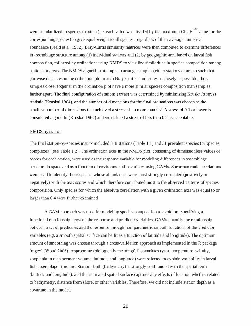
NMDS by station
The final station-by-species matrix included 318 stations (Table 1.1) and 31 prevalent species (or species
complexes) (see Table 1.2). The ordination axes in the NMDS plot, consisting of dimensionless values or
scores for each station, were used as the response variable for modeling differences in assemblage
structure in space and as a function of environmental covariates using GAMs. Spearman rank correlations
were used to identify those species whose abundances were most strongly correlated (positively or
negatively) with the axis scores and which therefore contributed most to the observed patterns of species
composition. Only species for which the absolute correlation with a given ordination axis was equal to or
larger than 0.4 were further examined.
A GAM approach was used for modeling species composition to avoid pre-specifying a
functional relationship between the response and predictor variables. GAMs quantify the relationship
between a set of predictors and the response through non-parametric smooth functions of the predictor
variables (e.g. a smooth spatial surface can be fit as a function of latitude and longitude). The optimum
amount of smoothing was chosen through a cross-validation approach as implemented in the R package
‘mgcv’ (Wood 2006). Appropriate (biologically meaningful) covariates (year, temperature, salinity,
zooplankton displacement volume, latitude, and longitude) were selected to explain variability in larval
fish assemblage structure. Station depth (bathymetry) is strongly confounded with the spatial term
(latitude and longitude), and the estimated spatial surface captures any effects of location whether related
to bathymetry, distance from shore, or other variables. Therefore, we did not include station depth as a
covariate in the model.
21
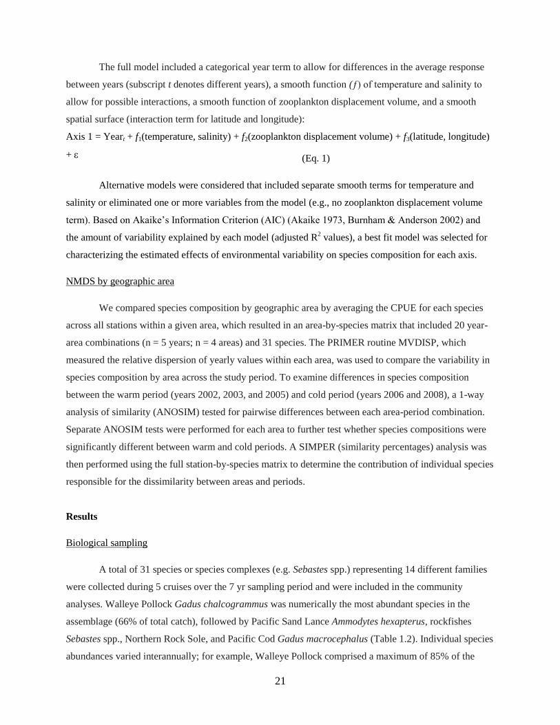
The full model included a categorical year term to allow for differences in the average response
between years (subscript t denotes different years), a smooth function (ƒ) of temperature and salinity to
allow for possible interactions, a smooth function of zooplankton displacement volume, and a smooth
spatial surface (interaction term for latitude and longitude):
Axis 1 = Yeart + f1(temperature, salinity) + f2(zooplankton displacement volume) + f3(latitude, longitude)
+ (Eq. 1)
Alternative models were considered that included separate smooth terms for temperature and
salinity or eliminated one or more variables from the model (e.g., no zooplankton displacement volume
term). Based on Akaike’s Information Criterion (AIC) (Akaike 1973, Burnham & Anderson 2002) and
the amount of variability explained by each model (adjusted R2 values), a best fit model was selected for
characterizing the estimated effects of environmental variability on species composition for each axis.
NMDS by geographic area
We compared species composition by geographic area by averaging the CPUE for each species
across all stations within a given area, which resulted in an area-by-species matrix that included 20 year-
area combinations (n = 5 years; n = 4 areas) and 31 species. The PRIMER routine MVDISP, which
measured the relative dispersion of yearly values within each area, was used to compare the variability in
species composition by area across the study period. To examine differences in species composition
between the warm period (years 2002, 2003, and 2005) and cold period (years 2006 and 2008), a 1-way
analysis of similarity (ANOSIM) tested for pairwise differences between each area-period combination.
Separate ANOSIM tests were performed for each area to further test whether species compositions were
significantly different between warm and cold periods. A SIMPER (similarity percentages) analysis was
then performed using the full station-by-species matrix to determine the contribution of individual species
responsible for the dissimilarity between areas and periods.
Results
Biological sampling
A total of 31 species or species complexes (e.g. Sebastes spp.) representing 14 different families
were collected during 5 cruises over the 7 yr sampling period and were included in the community
analyses. Walleye Pollock Gadus chalcogrammus was numerically the most abundant species in the
assemblage (66% of total catch), followed by Pacific Sand Lance Ammodytes hexapterus, rockfishes
Sebastes spp., Northern Rock Sole, and Pacific Cod Gadus macrocephalus (Table 1.2). Individual species
abundances varied interannually; for example, Walleye Pollock comprised a maximum of 85% of the
22
total catch in 2002 to a minimum of 29% in 2006 (Figure 1.3). Fish larvae were generally more abundant
in the warm years than in the cold years, especially Flathead Sole Hippoglossoides elassodon, northern
rock sole, and Pacific Sand Lance. Rare species, though not included in the analyses, were sampled in
either warm years (e.g. High Cockscomb Anoplarchus purpurescens and Greenland Halibut Reinhardtius
hippoglossoides) or cold years (e.g. Arctic Cod Boreogadus saida).
Physical environment sampling
The average water column temperature varied considerably between the warmer years of 2002,
2003, and 2005 (3.86, 4.75, and 4.16°C, respectively) and the colder years of 2006 and 2008 (3.39 and
2.0°C, respectively). This provided an environmental continuum against which to investigate changes in
larval fish species composition. Water mass characteristics were unique at slope, outer domain, and shelf
stations in cold years (Figure 1.2D), but the outer domain and shelf waters were not as clearly separated in
warm years (Figure 1.2C). Unimak Pass stations generally displayed similar characteristics to outer
domain waters; however, in 2002 and 2005, stations on the east side of Unimak Pass displayed
characteristics of shelf waters, whereas stations on the west side of Unimak Pass were more similar to
slope waters based on differences in salinity, indicating flow in both directions through Unimak Pass.
Community analyses
NMDS by station
The ordination of individual stations (Figure 1.4) condensed information on the abundance of each
species and afforded both community-level and species-specific gradients to be described across the study
area. GAMs illustrated 3 patterns in species composition that captured important habitat attributes for
larval fish distributions as described below. Spearman rank correlations with the NMDS axis scores
showed which individual species contributed most to the observed gradients. The first axis captured the
greatest amount of variability in species composition, which was corroborated by strong species’
correlations, both positive and negative. Several species were strongly positively correlated with the
second and third axes; however, no species were strongly negatively correlated with these axes (Table
1.3).
Generalized Additive Models
Axis 1
The first axis described a gradient between a slope assemblage (species positively correlated with Axis 1)
and a shelf assemblage (negatively correlated with Axis 1) that was resilient to interannual differences in
species abundances (Figure 1.5A). The slope assemblage was characterized by Sebastes spp. and
Atheresthes spp., as well as deeper-water species such as Pacific Blacksmelt (Bathylagus pacificus). In
23
contrast, the shelf assemblage was characterized by Alaska Plaice (Pleuronectes quadrituberculatus),
Pacific Sand Lance, Walleye Pollock, and Northern Rock Sole (Table 1.3).
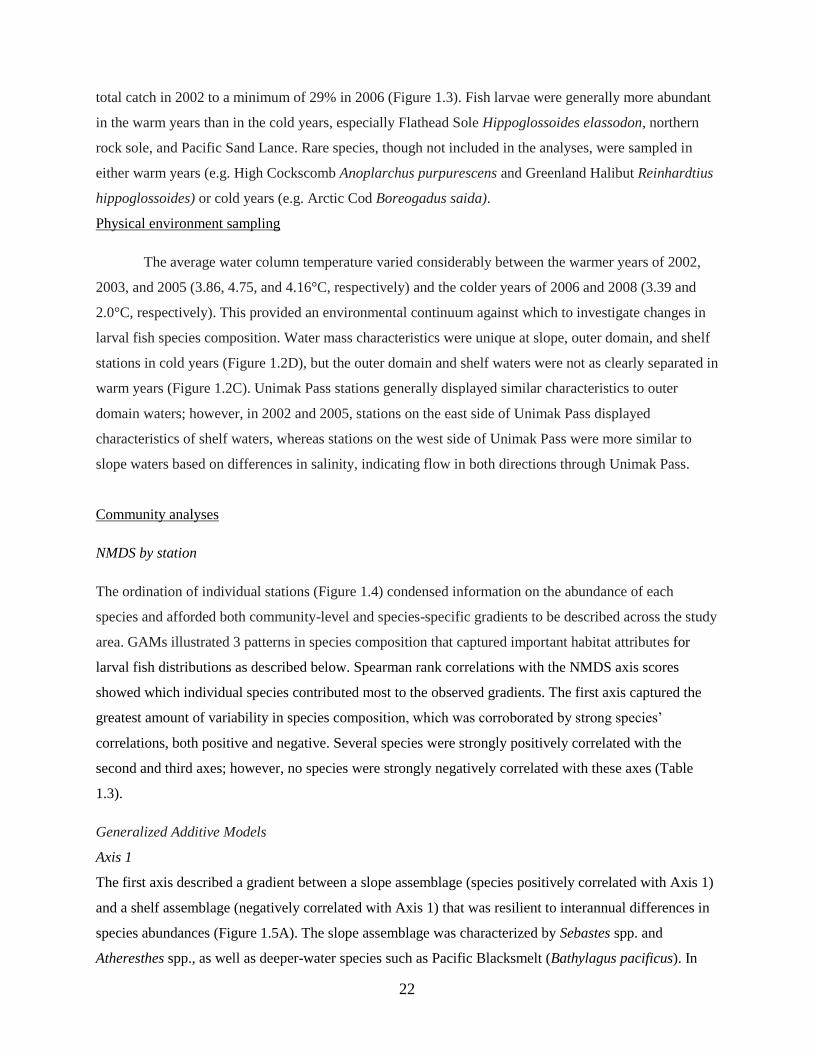
The best model for Axis 1 scores was described as:
Axis 1 ~ Yeart + f(Temperature, Salinity) + f(Latitude, Longitude) (Eq. 2)
and included a significant categorical year term denoting a difference in the average value of the response
among years, a significant smooth term of temperature and salinity, and a smooth spatial term (latitude
and longitude) (Table 1.4). Although temperature and salinity were confounded with the spatial term, the
latter largely captured residual variability not explained by either temperature or salinity. Zooplankton
displacement volume was not significant in the full model described by Eq. (1) and was dropped from the
best model. The model explained a significant proportion of the variability in species composition along
the first axis (adjusted R2
= 0.865; n = 318).
Both temperature and salinity had a strong influence on species composition (Figure 1.5B). The
slope assemblage (positive correlations) was more common at higher temperatures and at higher
salinities, while the shelf assemblage (negative correlations) was found at lower temperatures and
salinities, corroborating the cross-shelf spatial pattern described above. In addition, we found significant
variability in species composition among years (Figure 1.5C) that was not explained by local water mass
characteristics or spatial patterns. Species abundances were generally higher in warm years, driven by
shelf species such as Pacific sand lance, flathead sole, and northern rock sole
Axis 2
The second axis identified a plume of similar species composition originating in Unimak Pass and
extending onto the shelf. Figure 1.6A shows the average spatial pattern across all years, though the spatial
extent of the plume varied between years. Species strongly correlated with this plume of water included
flathead sole, Pacific Cod, and Northern Rock Sole (Table 1.3).
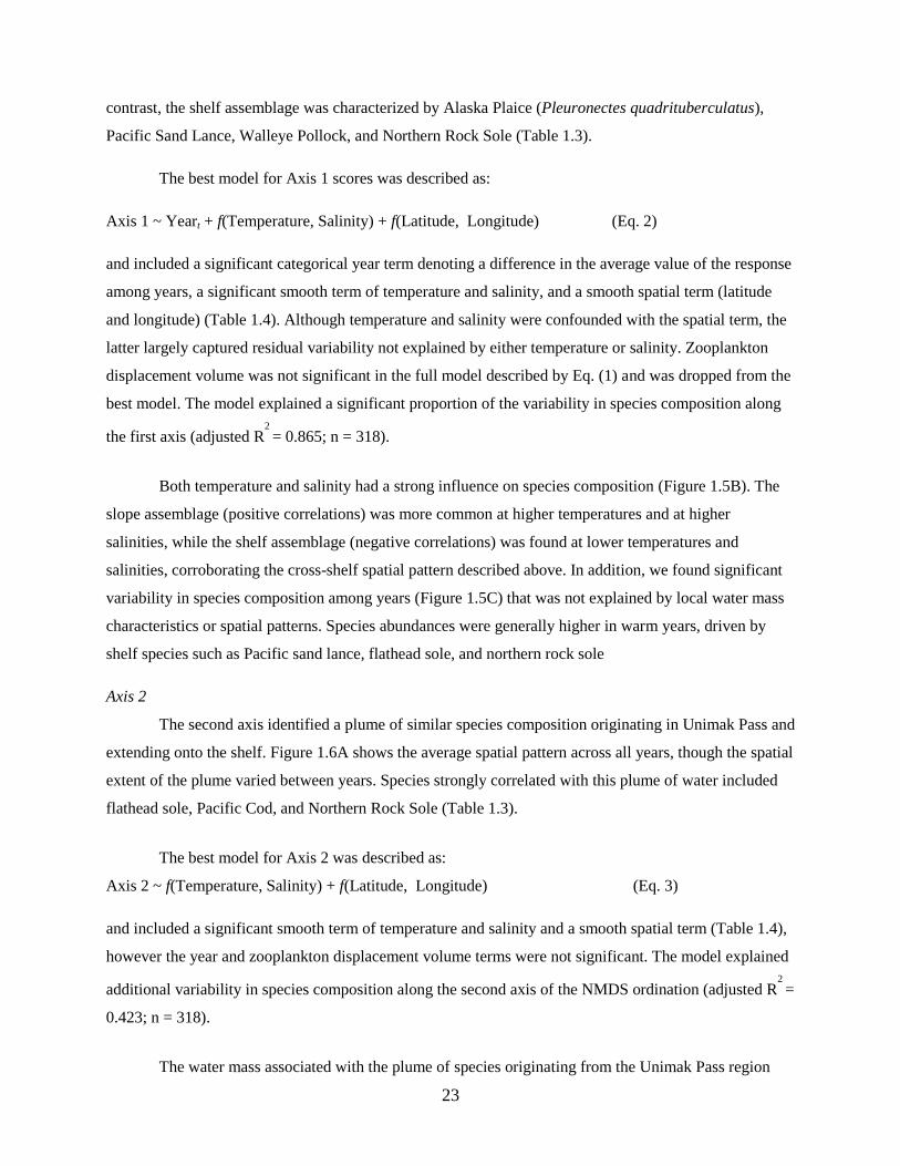
The best model for Axis 2 was described as:
Axis 2 ~ f(Temperature, Salinity) + f(Latitude, Longitude) (Eq. 3)
and included a significant smooth term of temperature and salinity and a smooth spatial term (Table 1.4),
however the year and zooplankton displacement volume terms were not significant. The model explained
additional variability in species composition along the second axis of the NMDS ordination (adjusted R2
=
0.423; n = 318).
The water mass associated with the plume of species originating from the Unimak Pass region
24
had warmer temperatures and lower salinities than surrounding waters (Figure 1.6B). The ACC carries
lower salinity waters from the Gulf of Alaska through Unimak Pass (Stabeno et al. 2002) and may have
influenced the spatial distribution (i.e. plume) of species assemblages. After accounting for the effects of
temperature and salinity, as well as the spatial pattern, there was no significant effect of year in Axis 2
scores, suggesting that interannual variability in species compositions was fully accounted for by
interannual differences in water mass characteristics.
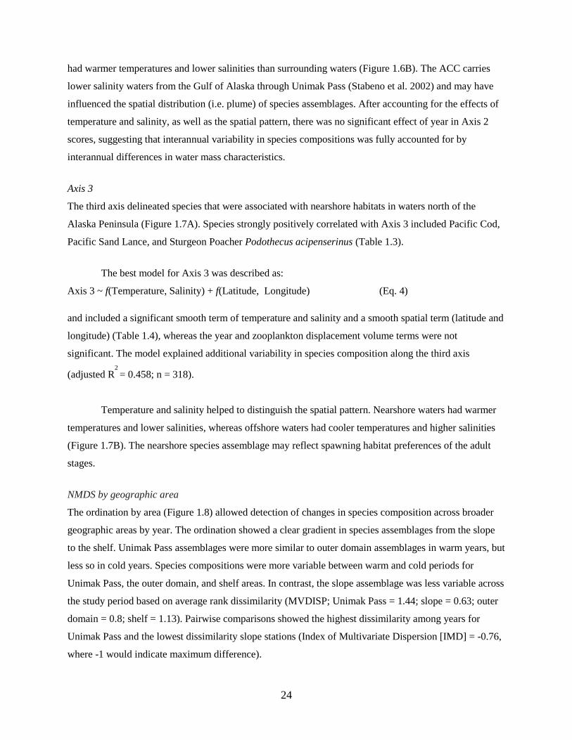
Axis 3
The third axis delineated species that were associated with nearshore habitats in waters north of the
Alaska Peninsula (Figure 1.7A). Species strongly positively correlated with Axis 3 included Pacific Cod,
Pacific Sand Lance, and Sturgeon Poacher Podothecus acipenserinus (Table 1.3).
The best model for Axis 3 was described as:
Axis 3 ~ f(Temperature, Salinity) + f(Latitude, Longitude) (Eq. 4)
and included a significant smooth term of temperature and salinity and a smooth spatial term (latitude and
longitude) (Table 1.4), whereas the year and zooplankton displacement volume terms were not
significant. The model explained additional variability in species composition along the third axis
(adjusted R2
= 0.458; n = 318).
Temperature and salinity helped to distinguish the spatial pattern. Nearshore waters had warmer
temperatures and lower salinities, whereas offshore waters had cooler temperatures and higher salinities
(Figure 1.7B). The nearshore species assemblage may reflect spawning habitat preferences of the adult
stages.
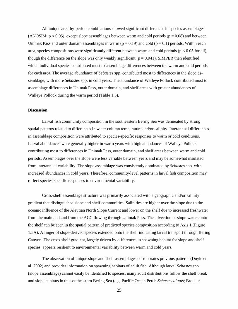
NMDS by geographic area
The ordination by area (Figure 1.8) allowed detection of changes in species composition across broader
geographic areas by year. The ordination showed a clear gradient in species assemblages from the slope
to the shelf. Unimak Pass assemblages were more similar to outer domain assemblages in warm years, but
less so in cold years. Species compositions were more variable between warm and cold periods for
Unimak Pass, the outer domain, and shelf areas. In contrast, the slope assemblage was less variable across
the study period based on average rank dissimilarity (MVDISP; Unimak Pass = 1.44; slope = 0.63; outer
domain = 0.8; shelf = 1.13). Pairwise comparisons showed the highest dissimilarity among years for
Unimak Pass and the lowest dissimilarity slope stations (Index of Multivariate Dispersion [IMD] = -0.76,
where -1 would indicate maximum difference).
25
All unique area-by-period combinations showed significant differences in species assemblages
(ANOSIM; p < 0.05), except slope assemblages between warm and cold periods (p = 0.08) and between
Unimak Pass and outer domain assemblages in warm (p = 0.19) and cold (p = 0.1) periods. Within each
area, species compositions were significantly different between warm and cold periods (p < 0.05 for all),
though the difference on the slope was only weakly significant (p = 0.041). SIMPER then identified
which individual species contributed most to assemblage differences between the warm and cold periods
for each area. The average abundance of Sebastes spp. contributed most to differences in the slope as-
semblage, with more Sebastes spp. in cold years. The abundance of Walleye Pollock contributed most to
assemblage differences in Unimak Pass, outer domain, and shelf areas with greater abundances of
Walleye Pollock during the warm period (Table 1.5).
Discussion
Larval fish community composition in the southeastern Bering Sea was delineated by strong
spatial patterns related to differences in water column temperature and/or salinity. Interannual differences
in assemblage composition were attributed to species-specific responses to warm or cold conditions.
Larval abundances were generally higher in warm years with high abundances of Walleye Pollock
contributing most to differences in Unimak Pass, outer domain, and shelf areas between warm and cold
periods. Assemblages over the slope were less variable between years and may be somewhat insulated
from interannual variability. The slope assemblage was consistently dominated by Sebastes spp. with
increased abundances in cold years. Therefore, community-level patterns in larval fish composition may
reflect species-specific responses to environmental variability.
Cross-shelf assemblage structure was primarily associated with a geographic and/or salinity
gradient that distinguished slope and shelf communities. Salinities are higher over the slope due to the
oceanic influence of the Aleutian North Slope Current and lower on the shelf due to increased freshwater
from the mainland and from the ACC flowing through Unimak Pass. The advection of slope waters onto
the shelf can be seen in the spatial pattern of predicted species composition according to Axis 1 (Figure
1.5A). A finger of slope-derived species extended onto the shelf indicating larval transport through Bering
Canyon. The cross-shelf gradient, largely driven by differences in spawning habitat for slope and shelf
species, appears resilient to environmental variability between warm and cold years.
The observation of unique slope and shelf assemblages corroborates previous patterns (Doyle et
al. 2002) and provides information on spawning habitats of adult fish. Although larval Sebastes spp.
(slope assemblage) cannot easily be identified to species, many adult distributions follow the shelf break
and slope habitats in the southeastern Bering Sea (e.g. Pacific Ocean Perch Sebastes alutus; Brodeur
26
2001). Juvenile Atheresthes spp., comprising Arrowtooth Flounder A. stomias and Kamchatka Flounder
A. evermanni, are widely distributed on the continental shelf and begin recruiting to the slope habitat after
about age-4 (Wilderbuer et al. 2009). In recent years, their abundance has increased, leading to a greater
trophic impact; adult Arrowtooth Flounder are known to be voracious predators on juvenile Walleye
Pollock (Livingston & Jurado-Molina 2000, Knoth & Foy 2008, Ianelli et al. 2009). Larval pollock,
however, were predominant in the shelf assemblage in our study, indicating spatial separation from adult
Arrowtooth Flounder and from larval aggregations of Atheresthes spp. over the slope. Alaska Plaice
spawn along the north side of the Alaska Peninsula in April and May, and eggs and larvae drift north and
northeast over the shelf (Duffy-Anderson et al. 2010). While the drift trajectories vary interannually, the
general current flow retains Alaska plaice within the shelf habitat.
The advection of ACC waters through Unimak Pass (Ladd et al. 2005) may affect the distribution
of larval fish on the southeastern Bering Sea shelf. Water in Unimak Pass is similar to the outer domain
water mass, especially in cold years, indicating directional flow of ACC water onto the outer Bering Sea
shelf. Warm years with greater inflow of ACC water (T. Royer unpubl. data) may result in increased
mixing and subsequent blending of water mass characteristics over the shelf (Figure 1.2C). In cold years,
inflow of ACC water is reduced, resulting in a clearer distinction of water masses (Figure 1.2D).
Species entrained in, or advected by, ACC waters within Unimak Pass and the Bering Sea shelf
included Pacific Cod and northern rock sole, with higher overall abundances of these species in warm
years. The trawling grounds around Unimak Pass are some of the most productive fishing areas for
Pacific Cod in the Bering Sea (Conners & Munro 2008), and just northeast of Unimak Pass is a major
spawning area (Shimada & Kimura 1994). Pacific Cod larvae caught in and near Unimak Pass in this
study may reflect these well-known spawning areas and/or reflect the contribution of Pacific Cod
spawned in the Gulf of Alaska to Bering Sea populations. Previous research on northern rock sole has
identified spawning areas west of Unimak Pass along the Aleutian Islands and in the Gulf of Alaska with
advection through Unimak Pass. Transport pathways follow the middle and outer shelf or flow eastward
along the Alaska Peninsula (Lanksbury et al. 2007). Differential survival of Northern Rock Sole depends
on transport to adequate nursery grounds in the coastal domain (Wilderbuer et al. 2002, Lanksbury et al.
2007). Unfortunately, our sampling design cannot resolve whether these larvae originated in the Gulf of
Alaska or were entrained in ACC waters within Unimak Pass and nearby spawning grounds. The impact
of Gulf of Alaska larvae on Bering Sea populations, and the degree to which the populations are con-
nected, are important ecological (i.e. competition, predation) and fisheries management (number of sub-
populations) questions. To address the connectedness of these populations, future work tracking larvae
from different spawning grounds using genetic markers, otolith microchemistry, or differential growth
rates could improve the resolution of Gulf of Alaska larval contributions to Bering Sea populations.
27
The importance of nearshore habitats to Pacific Cod, Bathymaster spp., and Pacific Sand Lance
could reflect preferred spawning grounds of adult fish (e.g. Pacific Cod; Shimada & Kimura 1994). The
onshore-offshore gradient in species composition was more difficult to interpret because correlations with
individual species’ CPUEs were weaker than for the other axes. In addition, the third NMDS axis
captured residual variability not already accounted for in the first or second axes. However, the
importance of nearshore habitat and an onshore-offshore gradient in species composition are biologically
reasonable; therefore, we believe our interpretation of this axis is realistic.
The 3 spatial patterns of larval fish assemblages identified from the NMDS ordination axes are
not exclusive; individual species can be correlated with more than one gradient, thereby capturing
different influences on larval distribution. For example, Pacific sand lance was strongly correlated with
the first and third axes. The first axis described Pacific sand lance as a shelf species, while the third axis
further associated larval sand lance with the nearshore environment of the shelf habitat. Pacific Cod was
correlated with the second and third axes. The second axis highlighted the importance of ACC waters in
the distribution of larval Pacific Cod while the third axis identified the nearshore environment as
important, likely due to the spawning preferences of adult fish.
The analytical approach of multivariate ordination followed by GAMs as an exploratory
regression technique successfully highlighted the main delineations of species compositions and modeled
the response of the assemblage to environmental covariates. However, caution should be used when
interpreting such results, as spurious (i.e. non-biologically relevant) outcomes are possible due to the
flexible nature of GAMs. We are confident in our interpretations of the model results based on current
knowledge of the Bering Sea ecosystem and believe our approach captured underlying mechanisms that
determine larval fish species compositions in the southeastern Bering Sea.
While the timing of surveys used for this study was consistent across years, differential
temperature effects on early life history events (e.g. spawning) could affect our interpretations. If colder
temperatures result in delayed adult spawning activities or reduced rates of ichthyoplankton development,
the fixed timing of our surveys could have been mismatched to the variable timing of larval production.
Further, the timing of front formation in the region can also affect the distribution of larvae. For example,
the Bering Sea Inner Front is a seasonally established hydrographic front that sets up in the vicinity of the
40 m isobath in spring and persists through late autumn (Schumacher & Stabeno 1998, Kachel et al.
2002). We hypothesize that if cold conditions persist over the shelf into late spring, the timing of the set
up of the Inner Front would be delayed, resulting in continued retention of larvae in northward moving
currents along the 100 and 200 m isobaths and potentially out of our east-west survey area (Lanksbury et
28
al. 2007).
The Oscillating Control Hypothesis (Hunt et al. 2002; revised in Hunt et al. 2011) provides a
theoretical framework within which to predict ecosystem responses to warm and cold regimes in the
southeastern Bering Sea. In warm regimes with early ice retreat, stratified waters maintain production
within the pelagic system (Mueter et al. 2006), resulting in enhanced survival of species such as Walleye
Pollock (Hunt & Stabeno 2002, Mueter et al. 2006, Moss et al. 2009). This is supported by the
observation in the current study of high larval Walleye Pollock abundances in the warm years of 2002,
2003, and 2005. However, recent data show that in warm regimes, larger zooplankton taxa (e.g. large
calanoid copepods and euphausiids) are less abundant, thus reducing growth rates and lipid reserves of
young-of-year Walleye Pollock and thereby increasing predation risk and decreasing overwinter survival
(Hunt et al. 2011). Therefore, a discontinuity exists between early spring conditions (i.e. water column
temperature and prey availability), larval abundance, and the abundance of age-1 Walleye Pollock
observed following the first winter. Although higher abundances of larval Walleye Pollock may not be
indicative of eventual year-class strength, community-level analyses may provide information on ecolo-
gical interactions affecting specific populations.
Our study was the first to look at changes in larval fish community composition within the
southeastern Bering Sea over a time period that included both warm and cold periods. Significant
differences in assemblage structure were detected, supporting the hypothesis that early life stages may be
primary indicators of environmental change. The biological shifts between warm and cold regimes are
difficult to predict due to direct and indirect species responses; a better understanding of non-linear
environmental effects will increase predictive and management capabilities. The eastern Bering Sea
Walleye Pollock fishery averaged 1.31 million tons annually between 2000 and 2009 (Ianelli et al. 2009),
representing the largest commercial fishery in the USA by weight. Therefore, it is important to understand
the mechanisms underlying interannual variability in this stock.
Acknowledgements
We thank the officers and crew of NOAA’s RVs ‘Miller Freeman’ and ‘Oscar Dyson’. Funding was
provided through NOAA’s NPCREP and EcoFOCI programs, as well as the North Pacific Research
Board (NPRB) Bering Sea Integrated Ecosystem Research Program (BSIERP). We thank 3 anonymous
reviewers for providing helpful comments that improved the manuscript. This research is contribution
EcoFOCI-0759 to NOAA’s Fisheries-Oceanography Coordinated Investigations, NPRB 285, and BEST-
BSIERP 17.
29
Literature Cited
Akaike H (1973) Information theory as an extension of the maximum likelihood principle. In BN Petrov
and F Csaki (eds) Second International Symposium on Information Theory. Akademiai Kiado,
Budapest, p. 267-281.
Bacheler NM, Ciannelli L, Bailey KM, Duffy-Anderson JT (2010) Spatial and temporal patterns of
Walleye Pollock (Theragra chalcogramma) spawning in the eastern Bering Sea inferred from egg
and larval distributions. Fish Oceanogr 19(2): 107-120.
Boeing WJ, Duffy-Anderson JT (2008) Ichthyoplankton dynamics and biodiversity in the Gulf of Alaska:
Responses to environmental change. Ecol Indicators 8: 292-302.
Brander KM, Blom G, Borges MF, Erzini K, Henderson G, MacKenzie BR, Mendes H, Santos AMP,
Toresen P (2003) Changes in fish distribution in the eastern North Atlantic: are we seeing a
coherent response to changing temperature? ICES Mar Sci Symp 219: 260-273.
Brodeur RD (2001) Habitat-specific distribution of Pacific ocean perch (Sebastes alutus) in Pribilof
Canyon, Bering Sea. Cont Shelf Res 21: 227-224.
Brodeur RD, Peterson WT, Auth TD, Soulen HL, Parnel MM, Emerson AA (2008) Abundance and
diversity of coastal fish larvae as indicators of recent changes in ocean and climate conditions in
the Oregon upwelling zone. Mar Ecol Prog Ser 366: 187-202.
Burnham KP, Anderson DR (2002) Model selection and multi-model inference: a practical information-
theoretic approach, Springer-Verlag, New York, NY.
Chavez FP, Messié M (2009) A comparison of Eastern Boundary Upwelling Ecosystems. Prog Oceanogr
83(1-4): 80-96.
Ciannelli L, Chan K-S, Bailey KM, Stenseth NC (2004) Nonadditive effects of the environment on the
survival of a large marine fish population. Ecology 85(12): 3418-3427.
Clarke KR, Gorley RN (2006) PRIMER v6: User manual/tutorial. PRIMER-E: Plymouth.
Coachman LK (1986) Circulation, water masses, and fluxes on the southeastern Bering Sea shelf. Cont
Shelf Res 5(1-2): 23-108.
Conners ME, Munro P (2008) Effects of commercial fishing on local abundance of Pacific cod (Gadus
macrocephalus) in the Bering Sea. Fish Bull 106: 281-292.
30
Coyle KO, Pinchuk AI, Eisner LB, Napp JM (2008) Zooplankton species composition, abundance and
biomass on the eastern Bering Sea shelf during summer: The potential role of water-column
stability and nutrients in structuring the zooplankton community. Deep-Sea Res II 55: 1775-1791.
Coyle KO, Eisner LB, Mueter FJ, Pinchuk AI, Janout MA, Cieciel KD, Farley EV, Andrews AG (2011)
Climate change in the southeastern Bering Sea: impacts on pollock stocks and implications for
the Oscillating Control Hypothesis. Fish Oceanogr. 20: 139-156.
Doyle MJ, Mier KL, Busby MS, Brodeur RD (2002) Regional variation in springtime ichthyoplankton
assemblages in the northeast Pacific Ocean. Prog Oceanogr 53: 247-281.
Doyle MJ, Picquelle SJ, Mier KL, Spillane MC, Bond NA (2009) Larval fish abundance and physical
forcing in the Gulf of Alaska, 1981-2003. Prog Oceanogr 80: 163-187.
Duffy-Anderson JT, Busby MS, Mier KL, Deliyanides CM, Stabeno PJ (2006) Spatial and temporal
patterns in summer ichthyoplankton assemblages on the eastern Bering Sea shelf 1996-2000.
Fish Oceanogr 15: 80-94.
Duffy-Anderson JT, Doyle MJ, Mier KL, Stabeno PJ, Wilderbuer TK (2010) Early life ecology of Alaska
plaice (Pleuronectes quadrituberculatus) in the eastern Bering Sea: seasonality, distribution, and
dispersal. J Sea Res 64: 3-14.
Field JG, Clarke KR, Warwick RM (1982) A practical strategy for analyzing multispecies distribution
patterns. Mar Ecol Prog Ser 8: 37-52.
Hare SR, Mantua NJ (2000) Empirical evidence for North Pacific regime shifts in 1977 and 1989. Prog
Oceanogr 47: 103-145.
Hunt GL Jr, Stabeno PJ (2002) Climate change and the control of energy flow in the southeastern Bering
Sea. Prog Oceanogr 55: 5-22.
Hunt GL Jr, Stabeno PJ, Walters G, Sinclair E, Brodeur RD, Napp JM, Bond NA (2002) Climate change
and control of the southeastern Bering Sea pelagic ecosystem. Deep-Sea Res Part II 49: 5821-
5853
Hunt Jr., G.L., Coyle, K.O., Eisner, L., Farley, E.V., Heintz, R., Mueter, F.J., Napp, J.M., Overland, J.E.,
Ressler, P.H., Salo, S., Stabeno, P.J., 2011. Climate impacts on eastern Bering Sea foodwebs: A
synthesis of new data and an assessment of the Oscillating Control Hypothesis. ICES J. Mar. Sci.
68(6): 1230-1243.
31
Ianelli JN, Barbeaux S, Honkalehto T, Kotwicki S, Aydin K, Williamson N (2009) Assessment of the
Walleye Pollock stock in the Eastern Bering Sea. In: Stock assessment and fishery evaluation
report for the groundfish resources of the Bering Sea/Aleutian Islands regions. North Pacific
Fishery Management Council, 605 W. 4th Ave., Suite 306, Anchorage, AK, p 49-148.
IPCC (Intergovernmental Panel on Climate Change) (2007) Climate Change 2007: the physical science
basis. Solomon S, Qin D, Manning M, Chen Z and others (eds) Contribution of Working Group I
to the Fourth Assessment Report of the Intergovernmental Panel on Climate Change. Cambridge
University Press, Cambridge.
Iverson RL, Coachman LK, Cooney RT, English TS, Goering JJ, Hunt GL Jr, Macauley MC, McRoy CP,
Reeburgh WS, Whitledge TE (1979) Ecological significance of fronts in the southeastern Bering
Sea. In RJ Livingston (ed) Ecological Processes in Coastal and Marine Systems. Plenum Press,
New York, NY. p. 437-466.
Kachel NB, Hunt GL Jr, Salo SA, Schumacher JD, Stabeno PJ, Whitledge TE (2002) Characteristics and
variability of the inner front of the southeastern Bering Sea. Deep-Sea Res Part II 49: 5889-5909.
Knoth BA, Foy RJ (2008) Temporal variability in the food habits of Arrowtooth Flounder (Atheresthes
stomias) in the western Gulf of Alaska. NOAA Tech Memo NMFS-AFSC 184.
Kruskal JB (1964) Multidimensional scaling by optimizing goodness of fit to a nonmetric hypothesis.
Psychometrika 29: 1-27.
Ladd C, Hunt GL Jr, Mordy CW, Salo SA, Stabeno PJ (2005) Marine environment of the eastern and
central Aleutian Islands. Fish Oceanogr 14(Suppl. 1): 22-38.
Lanksbury JA, Duffy-Anderson JT, Mier KL, Wilson MT (2005) Ichthyoplankton abundance,
distribution, and assemblage structure in the Gulf of Alaska during September 2000 and 2001. Est
Coast Shelf Sci 64: 775-785.
Lanksbury JA, Duffy-Anderson JT, Mier KL, Busby MS, Stabeno PJ (2007) Distribution and transport
patterns of northern rock sole, Lepidopsetta polyxystra, larvae in the southeastern Bering Sea.
Prog Oceanogr 72: 39-62.
Livingston PA, Jurado-Molina J (2000) A multispecies virtual populations analysis of the eastern Bering
Sea. J Mar Sci 57: 294-299.
Minchin PR (1987) An evaluation of the relative robustness of techniques for ecological ordination.
Vegetatio 69: 89-101.
32
Moss JH, Farley EV, Feldman AM, Ianelli JN (2009) Spatial distribution, energetic status, and food
habits of eastern Bering Sea age-0 Walleye Pollock. Trans Am Fish Soc 138: 497-505
Mueter FJ, Litzow MA (2008) Sea ice retreat alters the biogeography of the Bering Sea continental shelf.
Ecol Appl 18(2): 309-320.
Mueter FJ, Ladd C, Palmer MC, Norcross BL (2006) Bottom-up and top-down controls of walleye
pollock (Theragra chalcogramma) on the Eastern Bering Sea shelf. Prog Oceanogr 68:152–183.
Mueter FJ, Hunt GL Jr, Litzow MA (2007) The Eastern Bering Sea shelf: a highly productive seasonally
ice-covered sea. ICES CM2007/D:04, available at www.ices.dk/products/ CMdocs/CM-
2007/D/D0407.pdf.
Mueter FJ, Broms C, Drinkwater KF, Friedland KD, Hare JA, Hunt GL Jr, Melle W (2009) Ecosystem
responses to recent oceanographic variability in high-latitude Northern Hemisphere ecosystems.
Prog Oceanogr 81: 93-110.
Napp JM, Baier CT, Brodeur RD, Coyle KO, Shiga N, Mier K (2002) Interannual and decadal variability
in zooplankton communities of the southeast Bering Sea shelf. Deep-Sea Res II 49: 5991-6008.
Perry AL, Low PJ, Ellis JR, Reynolds JD (2005) Climate change and distribution shifts in marine fishes.
Science 308: 1912-1915.
Pörtner HO, Berdal B, Blust R, Brix O, Colosimo A, Wachter BD, Giuliani A, Johansen T, Fischer T,
Knust R, Lannig G, Naevdal G, Nedenes A, Nyhammer G, Sartoris FJ, Serendero I, Sirabella P,
Thorkildsen S, Zakhartsev M (2001) Climate induced temperature effects on growth
performance, fecundity and recruitment in marine fish: developing a hypothesis for cause and
effect relationships in Atlantic cod (Gadus morhua) and common eelpout (Zoarces viviparus).
Cont Shelf Res 21: 1975-1997.
Royer TC (1982) Coastal freshwater discharge in the Northeast Pacific. J Geophys Res 87(C3): 2017–
2021.
Schumacher JD, Stabeno PJ (1998) The continental shelf of the Bering Sea. In AR Robinson and KH
Brink (eds) The Sea: The global coastal ocean: regional studies and synthesis. John Wiley and
Sons, New York, NY. p. 789-822.
Shima M, Bailey KM (1994) Comparative analysis of ichthyoplankton sampling gear for early life stages
of walleye pollock (Theragra chalcogramma). Fish Oceanogr 3(1): 50-59.
33
Shimada AM, Kimura DK (1994) Seasonal movements of Pacific cod, Gadus macrocephalus, in the
eastern Bering Sea and adjacent waters based on tag-recapture data. Fish Bull 92: 800-816
Spencer PD (2008) Density-independent and density-dependent factors affecting temporal changes in
spatial distributions of eastern Bering Sea flatfish. Fish Oceanogr 17: 396-410.
Stabeno PJ, Bond NA, Kachel NB, Salo SA, Schumacher JD (2001) On the temporal variability of the
physical environment over the south-eastern Bering Sea. Fish Oceanogr 10(1): 81-98.
Stabeno PJ, Reed RK, Napp JM (2002) Transport through Unimak Pass, Alaska. Deep-Sea Res Part II 49:
5919-5930.
Stabeno PJ, Hunt GL Jr, Napp JM, Schumacher JD (2005) Physical forcing of ecosystem dynamics on the
Bering Sea shelf. In AR Robinson and KH Brink (eds) The Sea: The global coastal ocean:
Interdisciplinary regional studies and syntheses, Part B. Harvard University Press, Cambridge,
MA. p. 1177–1212.
Weingartner TJ, Danielson SL, Royer TC (2005) Freshwater variability and predictability in the Alaska
Coastal Current. Deep-Sea Res Part II 52: 169-191.
Wilderbuer TK, Hollowed AB, Ingraham WJ Jr, Spencer PD, Conners ME, Bond NA, Walters GE (2002)
Flatfish recruitment response to decadal climatic variability and ocean conditions in the eastern
Bering Sea. Prog Oceanogr 55: 235-247.
Wilderbuer TK, Nichol DG, Aydin K (2009) Arrowtooth Flounder. In: Stock assessment and fishery
evaluation report for the groundfish resources of the Bering Sea/Aleutian Islands regions. North
Pacific Fishery Management Council, Anchorage, AK, p 677-740.
Wood SN (2006) Generalized Additive Models: An introduction with R. Chapman & Hall/CRC, Boca
Raton, FL.
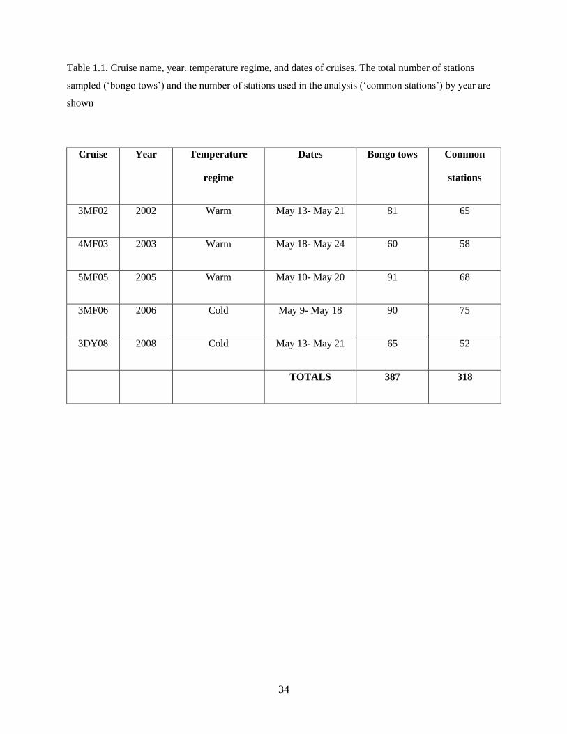
34
Table 1.1. Cruise name, year, temperature regime, and dates of cruises. The total number of stations
sampled (‘bongo tows’) and the number of stations used in the analysis (‘common stations’) by year are
shown
Cruise Year Temperature
regime
Dates Bongo tows Common
stations
3MF02 2002 Warm May 13- May 21 81 65
4MF03 2003 Warm May 18- May 24 60 58
5MF05 2005 Warm May 10- May 20 91 68
3MF06 2006 Cold May 9- May 18 90 75
3DY08 2008 Cold May 13- May 21 65 52
TOTALS 387 318
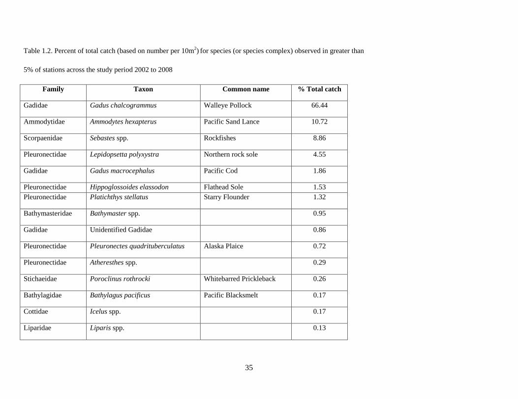
35
Table 1.2. Percent of total catch (based on number per 10m2)
for species (or species complex) observed in greater than
5% of stations across the study period 2002 to 2008
Family Taxon Common name % Total catch
Gadidae Gadus chalcogrammus Walleye Pollock 66.44
Ammodytidae Ammodytes hexapterus Pacific Sand Lance 10.72
Scorpaenidae Sebastes spp. Rockfishes 8.86
Pleuronectidae Lepidopsetta polyxystra Northern rock sole 4.55
Gadidae Gadus macrocephalus Pacific Cod 1.86
Pleuronectidae Hippoglossoides elassodon Flathead Sole 1.53
Pleuronectidae Platichthys stellatus Starry Flounder 1.32
Bathymasteridae Bathymaster spp. 0.95
Gadidae Unidentified Gadidae 0.86
Pleuronectidae Pleuronectes quadrituberculatus Alaska Plaice 0.72
Pleuronectidae Atheresthes spp. 0.29
Stichaeidae Poroclinus rothrocki Whitebarred Prickleback 0.26
Bathylagidae Bathylagus pacificus Pacific Blacksmelt 0.17
Cottidae Icelus spp. 0.17
Liparidae Liparis spp. 0.13
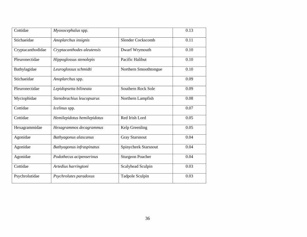
36
Cottidae Myoxocephalus spp. 0.13
Stichaeidae Anoplarchus insignis Slender Cockscomb 0.11
Cryptacanthodidae Cryptacanthodes aleutensis Dwarf Wrymouth 0.10
Pleuronectidae Hippoglossus stenolepis Pacific Halibut 0.10
Bathylagidae Leuroglossus schmidti Northern Smoothtongue 0.10
Stichaeidae Anoplarchus spp. 0.09
Pleuronectidae Lepidopsetta bilineata Southern Rock Sole 0.09
Myctophidae Stenobrachius leucopsarus Northern Lampfish 0.08
Cottidae Icelinus spp. 0.07
Cottidae Hemilepidotus hemilepidotus Red Irish Lord 0.05
Hexagrammidae Hexagrammos decagrammus Kelp Greenling 0.05
Agonidae Bathyagonus alascanus Gray Starsnout 0.04
Agonidae Bathyagonus infraspinatus Spinycheek Starsnout 0.04
Agonidae Podothecus acipenserinus Sturgeon Poacher 0.04
Cottidae Artedius harringtoni Scalyhead Sculpin 0.03
Psychrolutidae Psychrolutes paradoxus Tadpole Sculpin 0.03
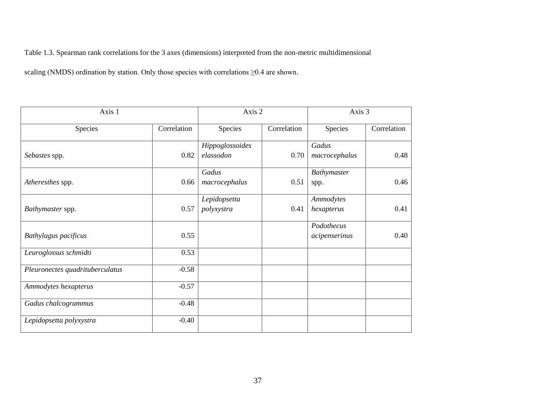
37
Table 1.3. Spearman rank correlations for the 3 axes (dimensions) interpreted from the non-metric multidimensional
scaling (NMDS) ordination by station. Only those species with correlations ≥0.4 are shown.
Axis 1 Axis 2 Axis 3
Species Correlation Species Correlation Species Correlation
Sebastes spp. 0.82
Hippoglossoides
elassodon 0.70
Gadus
macrocephalus 0.48
Atheresthes spp. 0.66
Gadus
macrocephalus 0.51
Bathymaster
spp. 0.46
Bathymaster spp. 0.57
Lepidopsetta
polyxystra 0.41
Ammodytes
hexapterus 0.41
Bathylagus pacificus 0.55
Podothecus
acipenserinus 0.40
Leuroglossus schmidti 0.53
Pleuronectes quadrituberculatus -0.58
Ammodytes hexapterus -0.57
Gadus chalcogrammus -0.48
Lepidopsetta polyxystra -0.40
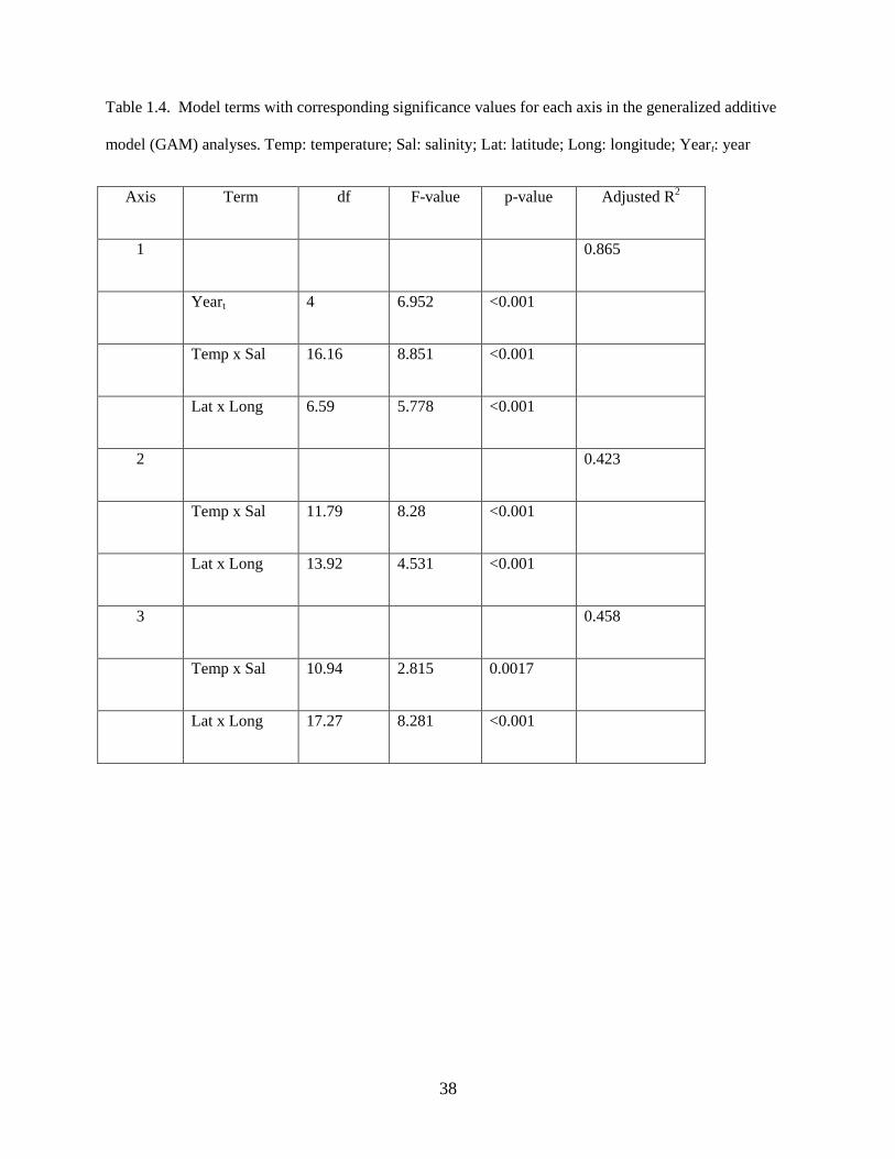
38
Table 1.4. Model terms with corresponding significance values for each axis in the generalized additive
model (GAM) analyses. Temp: temperature; Sal: salinity; Lat: latitude; Long: longitude; Yeart: year
Axis Term df F-value p-value Adjusted R2
1 0.865
Yeart 4 6.952 <0.001
Temp x Sal 16.16 8.851 <0.001
Lat x Long 6.59 5.778 <0.001
2 0.423
Temp x Sal 11.79 8.28 <0.001
Lat x Long 13.92 4.531 <0.001
3 0.458
Temp x Sal 10.94 2.815 0.0017
Lat x Long 17.27 8.281 <0.001
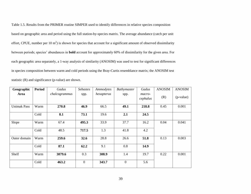
39
Table 1.5. Results from the PRIMER routine SIMPER used to identify differences in relative species composition
based on geographic area and period using the full station-by-species matrix. The average abundance (catch per unit
effort, CPUE, number per 10 m2) is shown for species that account for a significant amount of observed dissimilarity
between periods; species’ abundances in bold account for approximately 60% of dissimilarity for the given area. For
each geographic area separately, a 1-way analysis of similarity (ANOSIM) was used to test for significant differences
in species composition between warm and cold periods using the Bray-Curtis resemblance matrix; the ANOSIM test
statistic (R) and significance (p-value) are shown.
Geographic
Area
Period Gadus
chalcogrammus
Sebastes
spp.
Ammodytes
hexapterus
Bathymaster
spp.
Gadus
macro-
cephalus
ANOSIM
(R)
ANOSIM
(p-value)
Unimak Pass Warm 270.8 46.9 66.5 49.1 218.8 0.45 0.001
Cold 8.1 73.1 19.6 2.1 24.5
Slope Warm 67.4 495.3 33.9 37.7 16.2 0.04 0.041
Cold 48.5 717.5 1.3 41.8 4.2
Outer domain Warm 259.6 32.6 28.8 26.6 51.8 0.13 0.003
Cold 87.1 62.2 9.1 0.8 14.9
Shelf Warm 3079.6 0.3 308.9 1.4 19.7 0.22 0.001
Cold 463.2 0 343.7 0 5.6
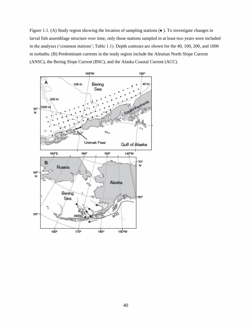
40
Figure 1.1. (A) Study region showing the location of sampling stations (). To investigate changes in
larval fish assemblage structure over time, only those stations sampled in at least two years were included
in the analyses (‘common stations’; Table 1.1). Depth contours are shown for the 40, 100, 200, and 1000
m isobaths. (B) Predominant currents in the study region include the Aleutian North Slope Current
(ANSC), the Bering Slope Current (BSC), and the Alaska Coastal Current (ACC).
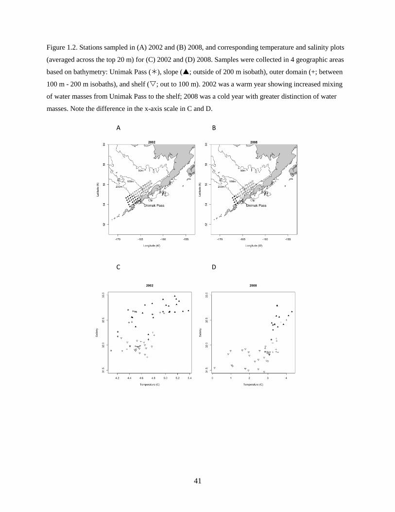
41
Figure 1.2. Stations sampled in (A) 2002 and (B) 2008, and corresponding temperature and salinity plots
(averaged across the top 20 m) for (C) 2002 and (D) 2008. Samples were collected in 4 geographic areas
based on bathymetry: Unimak Pass (), slope (; outside of 200 m isobath), outer domain (+; between
100 m - 200 m isobaths), and shelf (; out to 100 m). 2002 was a warm year showing increased mixing
of water masses from Unimak Pass to the shelf; 2008 was a cold year with greater distinction of water
masses. Note the difference in the x-axis scale in C and D.
A B
C D
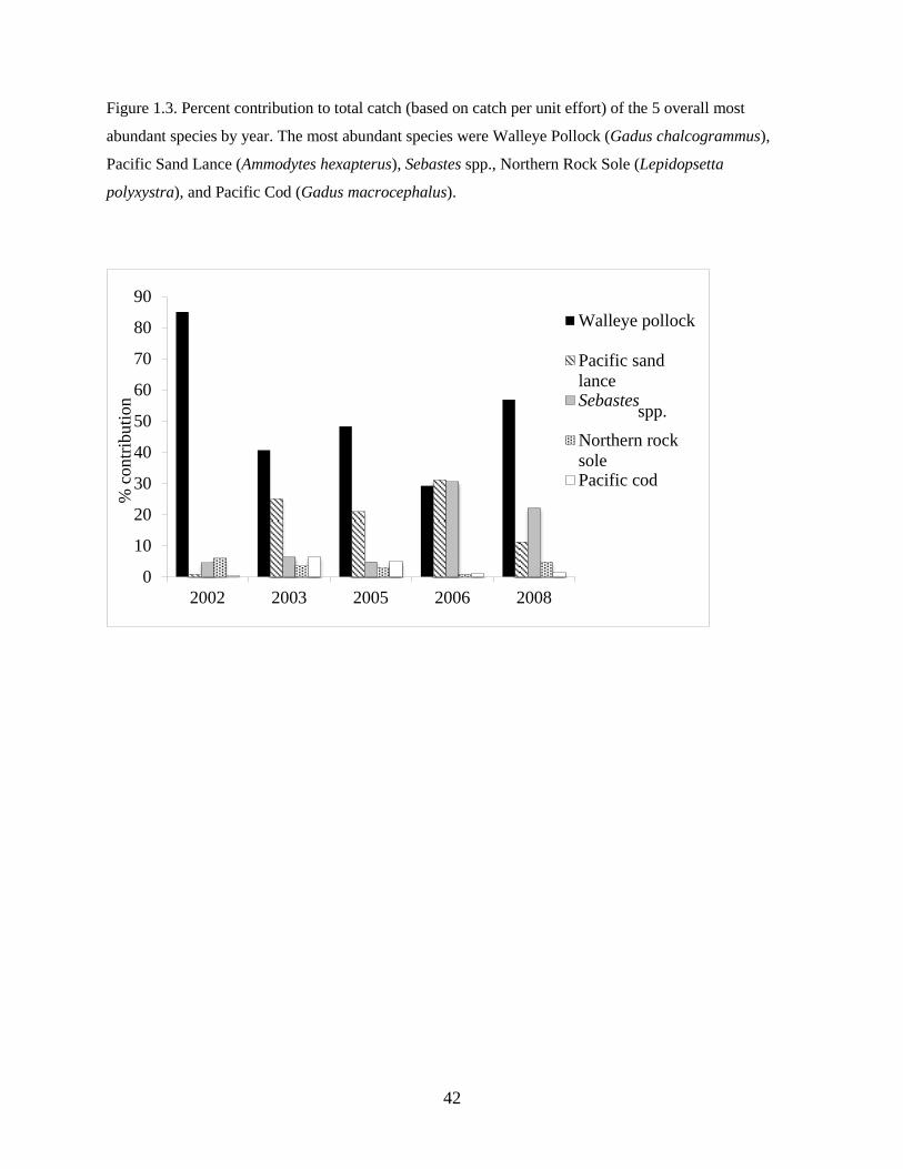
42
Figure 1.3. Percent contribution to total catch (based on catch per unit effort) of the 5 overall most
abundant species by year. The most abundant species were Walleye Pollock (Gadus chalcogrammus),
Pacific Sand Lance (Ammodytes hexapterus), Sebastes spp., Northern Rock Sole (Lepidopsetta
polyxystra), and Pacific Cod (Gadus macrocephalus).
0
10
20
30
40
50
60
70
80
90
2002 2003 2005 2006 2008
% c
ontr
ibuti
on
Walleye pollock
Pacific sand
lanceSebastes
Northern rock
solePacific cod
spp.
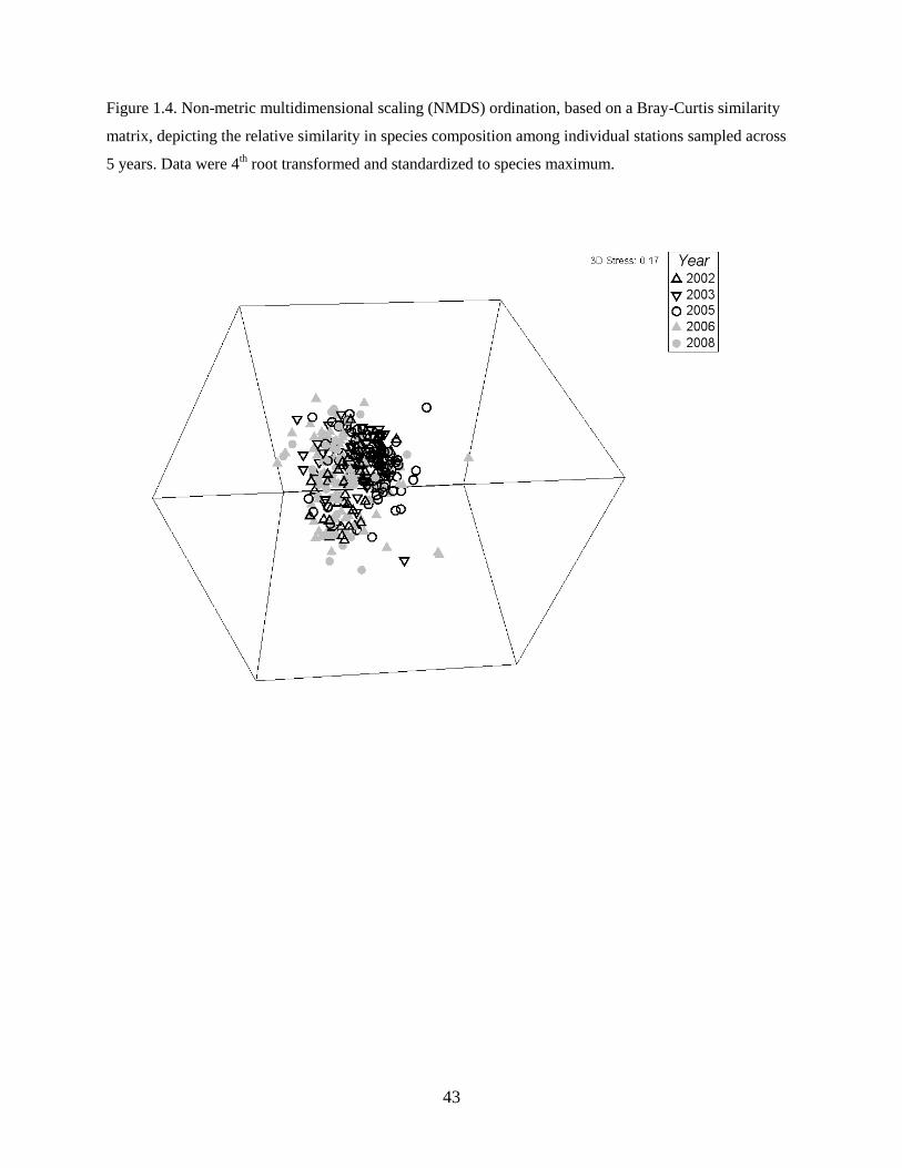
43
Figure 1.4. Non-metric multidimensional scaling (NMDS) ordination, based on a Bray-Curtis similarity
matrix, depicting the relative similarity in species composition among individual stations sampled across
5 years. Data were 4th root transformed and standardized to species maximum.
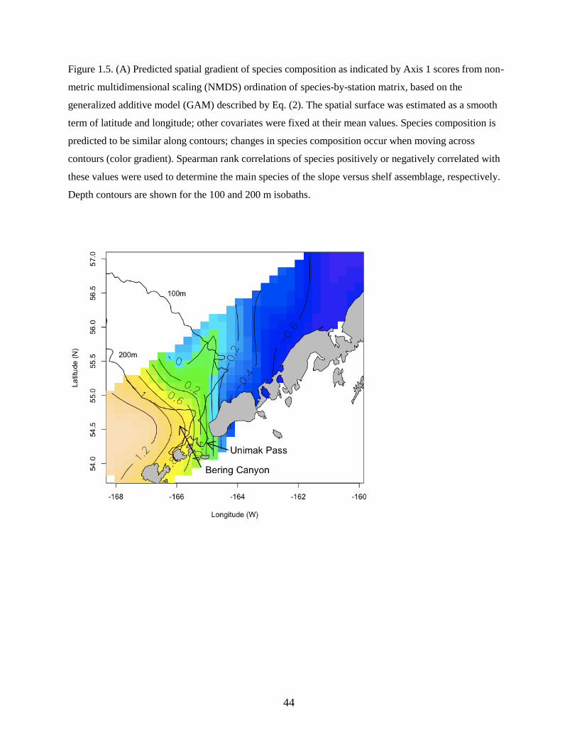
44
Figure 1.5. (A) Predicted spatial gradient of species composition as indicated by Axis 1 scores from non-
metric multidimensional scaling (NMDS) ordination of species-by-station matrix, based on the
generalized additive model (GAM) described by Eq. (2). The spatial surface was estimated as a smooth
term of latitude and longitude; other covariates were fixed at their mean values. Species composition is
predicted to be similar along contours; changes in species composition occur when moving across
contours (color gradient). Spearman rank correlations of species positively or negatively correlated with
these values were used to determine the main species of the slope versus shelf assemblage, respectively.
Depth contours are shown for the 100 and 200 m isobaths.
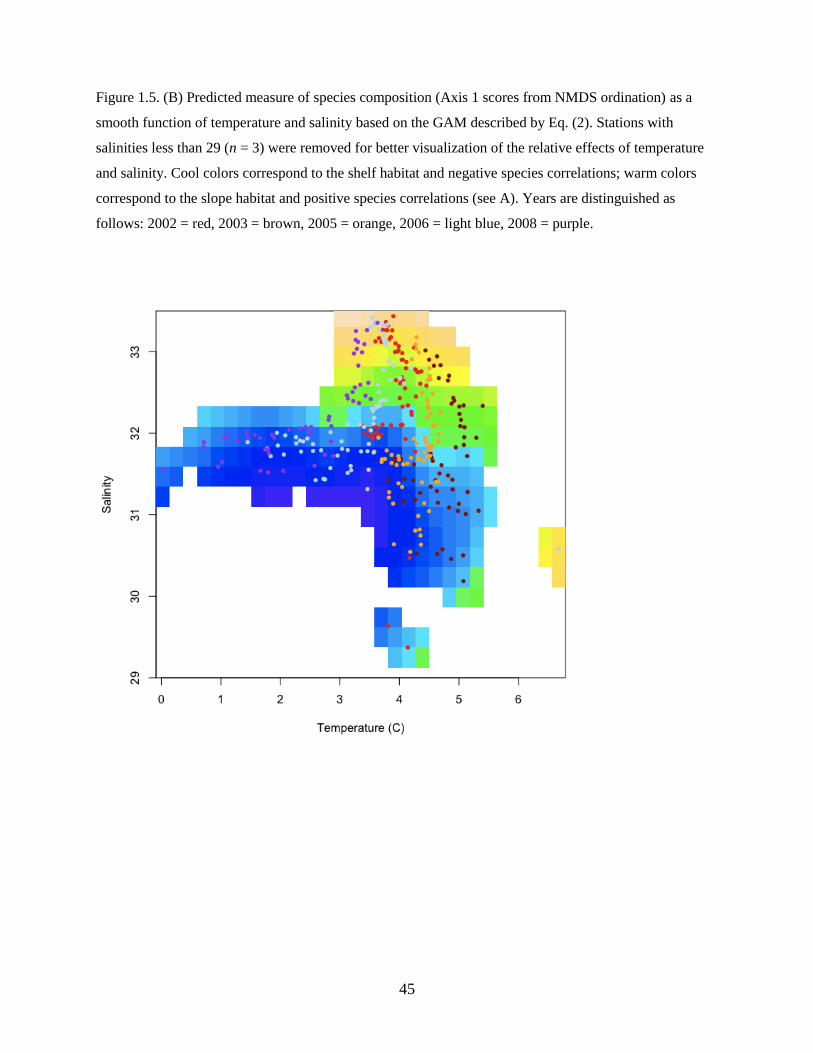
45
Figure 1.5. (B) Predicted measure of species composition (Axis 1 scores from NMDS ordination) as a
smooth function of temperature and salinity based on the GAM described by Eq. (2). Stations with
salinities less than 29 (n = 3) were removed for better visualization of the relative effects of temperature
and salinity. Cool colors correspond to the shelf habitat and negative species correlations; warm colors
correspond to the slope habitat and positive species correlations (see A). Years are distinguished as
follows: 2002 = red, 2003 = brown, 2005 = orange, 2006 = light blue, 2008 = purple.
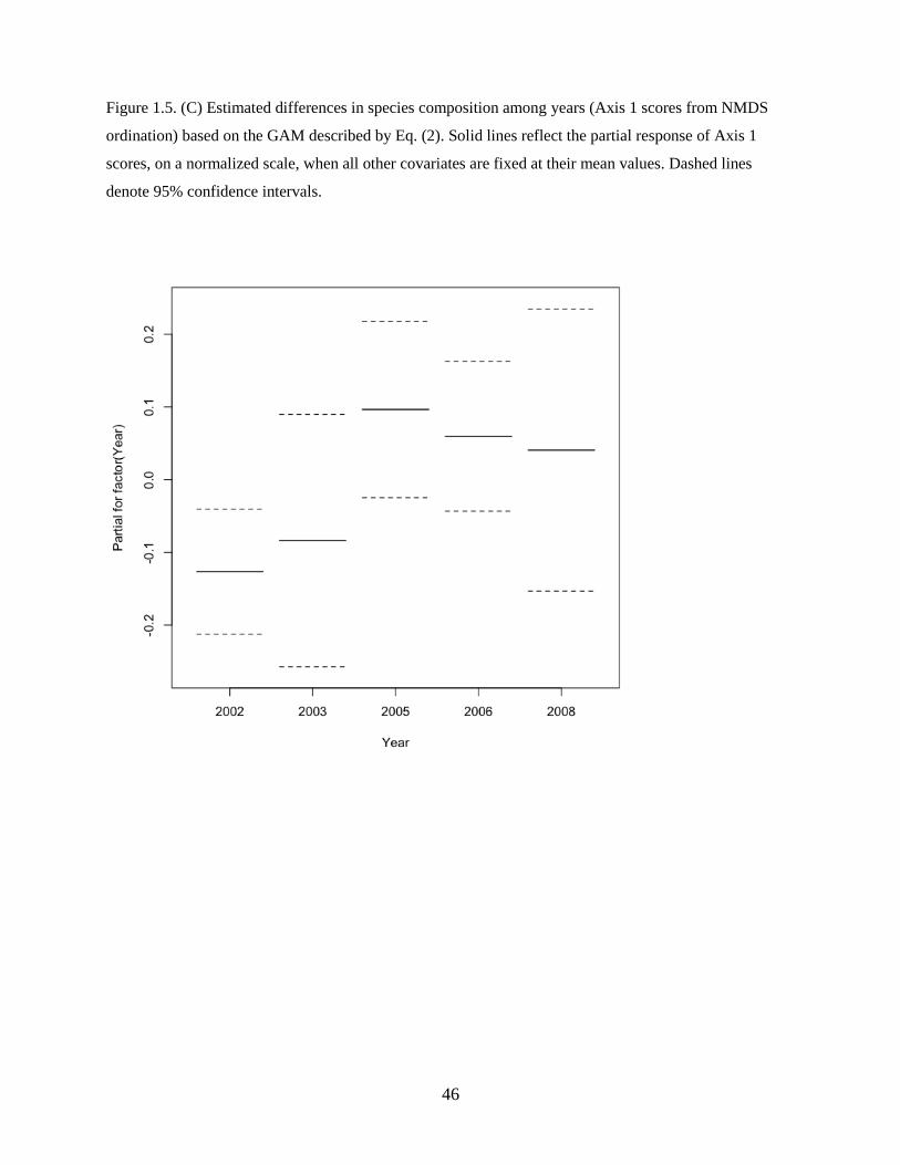
46
Figure 1.5. (C) Estimated differences in species composition among years (Axis 1 scores from NMDS
ordination) based on the GAM described by Eq. (2). Solid lines reflect the partial response of Axis 1
scores, on a normalized scale, when all other covariates are fixed at their mean values. Dashed lines
denote 95% confidence intervals.
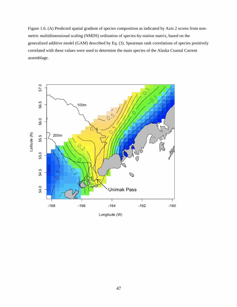
47
Figure 1.6. (A) Predicted spatial gradient of species composition as indicated by Axis 2 scores from non-
metric multidimensional scaling (NMDS) ordination of species-by-station matrix, based on the
generalized additive model (GAM) described by Eq. (3). Spearman rank correlations of species positively
correlated with these values were used to determine the main species of the Alaska Coastal Current
assemblage.
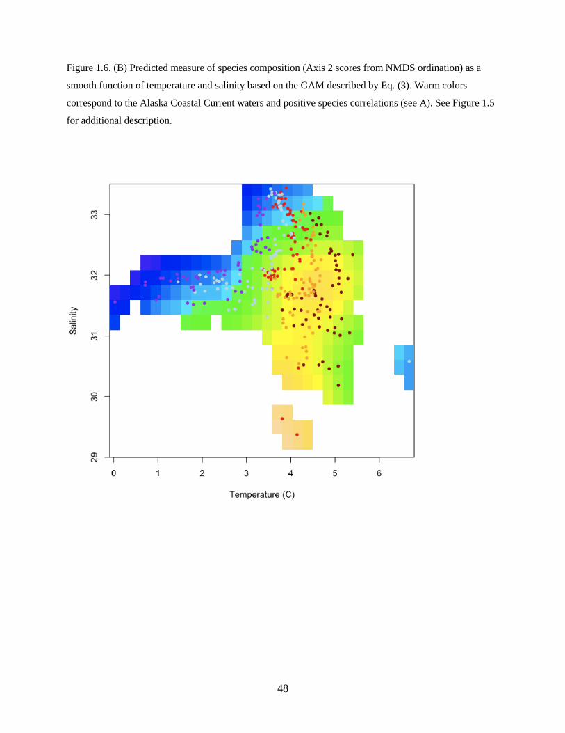
48
Figure 1.6. (B) Predicted measure of species composition (Axis 2 scores from NMDS ordination) as a
smooth function of temperature and salinity based on the GAM described by Eq. (3). Warm colors
correspond to the Alaska Coastal Current waters and positive species correlations (see A). See Figure 1.5
for additional description.
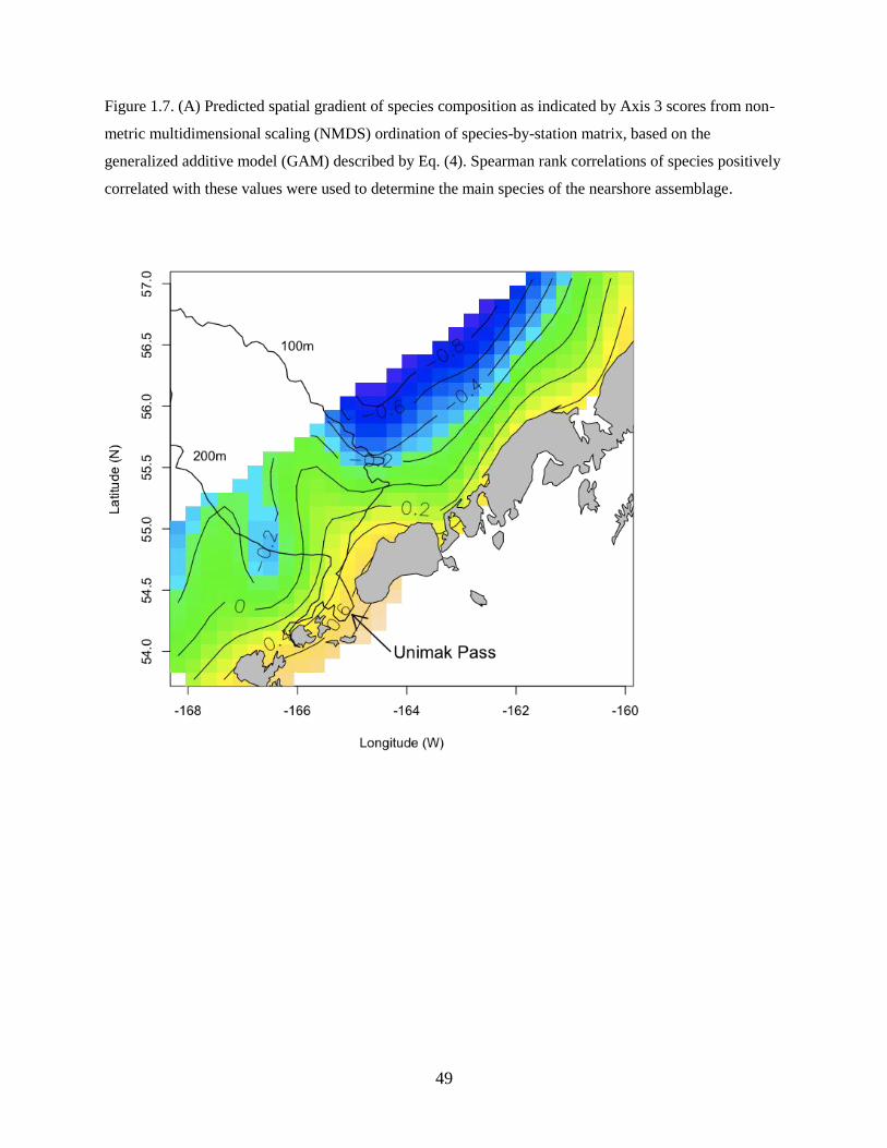
49
Figure 1.7. (A) Predicted spatial gradient of species composition as indicated by Axis 3 scores from non-
metric multidimensional scaling (NMDS) ordination of species-by-station matrix, based on the
generalized additive model (GAM) described by Eq. (4). Spearman rank correlations of species positively
correlated with these values were used to determine the main species of the nearshore assemblage.
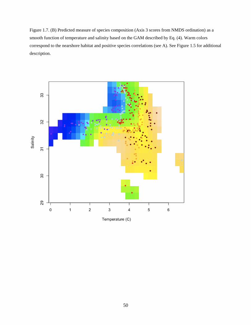
50
Figure 1.7. (B) Predicted measure of species composition (Axis 3 scores from NMDS ordination) as a
smooth function of temperature and salinity based on the GAM described by Eq. (4). Warm colors
correspond to the nearshore habitat and positive species correlations (see A). See Figure 1.5 for additional
description.
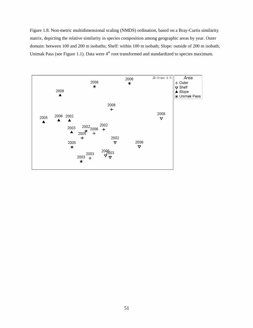
51
Figure 1.8. Non-metric multidimensional scaling (NMDS) ordination, based on a Bray-Curtis similarity
matrix, depicting the relative similarity in species composition among geographic areas by year. Outer
domain: between 100 and 200 m isobaths; Shelf: within 100 m isobath; Slope: outside of 200 m isobath;
Unimak Pass (see Figure 1.1). Data were 4th root transformed and standardized to species maximum.
52
Chapter 2: Influence of environment on Walleye Pollock eggs, larvae, and
juveniles in the southeastern Bering Sea
Tracey I. Smart1, Janet T. Duffy-Anderson
2, John K. Horne
1, Edward V. Farley
3, Christopher D. Wilson
2,
and Jeffrey M. Napp2
1School of Aquatic and Fishery Sciences, University of Washington, Box 355020, Seattle, WA 98195,
USA
2RACE Division, Recruitment Processes Program, Alaska Fisheries Science Center, National Marine
Fisheries Service, NOAA, 7600 Sand Point Way, Seattle, WA 98115, USA
3Auke Bay Laboratories, Alaska Fisheries Science Center, National Marine Fisheries Service, NOAA,
17109 Point Lena Loop Rd., Juneau, AK 99801, USA
Citation: Smart, T., Duffy-Anderson, J.T., Horne, J., Farley, E., Wilson, C., and Napp, J. 2012. Influence
of environment on Walleye Pollock eggs, larvae, and juveniles in the Southeastern Bering Sea. Deep-Sea
Research II: Topical Studies in Oceanography. 65-70: 196-207.
53
Abstract
We examined the influence of environmental conditions on Walleye Pollock (Gadus
chalcogrammus) early life history in discrete stages at two ecological scales using a 17-year time series
from the southeastern Bering Sea. Generalized additive models (GAMs) were used to quantify
relationships between Walleye Pollock stages (eggs, yolksac larvae, preflexion larvae, late larvae, and
juveniles), the fine-resolution environment (temperature, wind speed, salinity, and copepod
concentration), and the broad-resolution environment (annual spawning stock biomass, temperature,
zooplankton biomass, and wind mixing). Early stages (eggs, yolksac larvae, and preflexion larvae) were
associated with high spawning stock biomass, while late stages (late larvae and juveniles) were not
associated with spawning stock biomass. The influence of temperature increased with ontogeny: high egg
abundance was associated with temperatures from -2 to 7 oC and negative annual temperature anomalies
and high juvenile abundance was associated with temperatures from 4 to 12 oC and positive temperature
anomalies. Winds enhanced the transport of early stages from spawning locations to shallower sampling
depths, but did not affect feeding stages (preflexion larvae, late larvae, and juveniles) in a manner
consistent with the encounter-turbulence hypothesis. Feeding stages were positively associated with
localized copepod concentrations but not zooplankton biomass anomaly, suggesting that the localized
measurements of potential prey is a better indicator compared to broad-scale conditions measured in areas
where these stages do not necessarily occur. Broad-resolution covariates, however, explained a greater
portion of the overall variation than did fine-resolution models. Of the environmental conditions
examined, temperature explained more variation in abundance of Walleye Pollock early life stages than
any other covariate. Temperature is likely a major driving force structuring variability in populations of
Walleye Pollock in their first year of life, acting directly upon them and indirectly upon their physical
habitat and prey community.
54
Introduction
The southeastern Bering Sea (SEBS) is part of a productive, high-latitude ecosystem that provides
critical spawning and larval habitat for demersal fish species. In particular, the SEBS serves as important
spawning, nursery, and forage habitat for Walleye Pollock (Gadus chalcogrammus, hereafter referred to
as pollock), a target species for one of the world’s largest commercial fisheries (FAO, 2007). Pollock
account for about 60 % of the total landings of groundfish in Alaskan waters (Ianelli et al., 2009) and also
serve key ecological roles acting as top predators, prey for other top predators, and consumers of
zooplankton. For Bering Sea pollock, female spawning biomass has fluctuated widely over the last four
decades (from 0.85 to 4.1 million metric tons) and recruitment variability in the species is high, similar to
other gadids (Ianelli et al., 2009). In the Gulf of Alaska (GOA) spawning biomass changes the initial
production of eggs and availability of hatched larvae (Bacheler et al., 2009). Climate and hydrography
influence the extent of transport from spawning grounds (Ciannelli et al., 2005; Wilson, 2009) and the
survival and growth of larvae and juveniles (Porter et al., 2005; Logerwell et al., 2010).
Recently, Ciannelli et al. (2004) used a stage-specific approach to determine the density-
dependent structure of pollock survival in the GOA, and Bacheler et al. (2010) used a stage-specific
approach to define the temporal distributions of pollock eggs and early stage larvae over the SEBS shelf.
Bacheler et al. (2010) identified three unique spawning areas with distinct egg and early larval
phenologies, but did not examine interannual or seasonal changes in the physical environment
experienced by eggs, larvae, or juveniles. Both studies demonstrated the importance of stage-specific
responses in our ability to account for population trends and variation.
It is probable that a combination of biological and oceanographic conditions influences all fish
life history stages and that the importance of any factor varies among stages. Objectives of the current
study were to identify key factors that affect pollock early life stage (ELS) abundances in the Bering Sea
and quantify the influence these factors have during the first year of development. Of course,
environmental conditions may act on growth and survival of ELS either singly or in combination. For
example, pollock egg development, time to hatch, and use of yolk reserves are controlled by temperature
(Blood, 2002). Early larvae are more successful under both moderate wind-driven mixing conditions and
good prey conditions (Walline, 1985; Bailey and Macklin, 1994; Mueter et al., 2006). Olla et al. (1996)
suggested that mixing and temperature interact to determine larval pollock feeding success and
subsequent growth and survival. Prey availability and temperature also interact to determine prey capture
rates and survival of larvae, particularly when prey is scarce (Fukuchi, 1976). Adult pollock biomass,
temperature, and wind conditions influence early juvenile and age-1 abundances in the Bering Sea
(Wespestad et al., 2000; Duffy-Anderson et al., 2005; Mueter et al., 2006).
55
Environmental data are available over a range of spatial and temporal resolutions in the northeast
Pacific. This range enables the examination of the relative importance of biological and physical factors
at fine- and broad-scales. We define fine-resolution environmental data as those factors measured in
association with individual ichthyoplankton tows at daily or weekly frequencies. Broad-resolution
environmental data are those factors integrated over space and time across the eastern Bering Sea and
within months or years. Broad-resolution indices have the advantage of larger sample sizes, while fine-
resolution measurements address the immediate environmental conditions, which are more relevant to
growth and survival of an early stage pollock. For Bering Sea pollock, there has been no comprehensive
examination of all ELS and the relative importance of environmental conditions at each stage. The
potential influence of the adult population on pollock ELS abundances was accounted for by testing for
temperature-induced changes in spawn timing, with may influence which ELS we capture during surveys,
and by including a spawning population index, which can constrain the number of ELS produced
annually. The influence of environmental conditions on pollock ELS was compared to the influence of
spatial position and time of year, which have been identified as important predictors of pollock ELS
abundance in the Bering Sea (Bacheler et al., 2010).
Methods
Ichthyoplankton sampling
Depth-integrated abundance (number collected per 10 m2 sampled) of pollock ELS were
measured during ichthyoplankton surveys conducted by NOAA’s Alaska Fisheries Science Center
(AFSC, see Matarese et al., 2003). Surveys targeted pollock spawning grounds, areas adjacent to
spawning grounds, and areas of downstream transport. Catch records were selected to include only
samples south of 60 N latitude and east of the Aleutian Basin as samples were collected rarely outside of
this area (Figure 2.1). Catch records also were limited to those between February and October due to
limited sampling outside of this window and alignment with the spawning season (Bacheler et al., 2010).
Surveys within the target area and dates occurred in 17 years within the time series (1988, 1991, 1992,
1994-2000, and 2002-2008, Table 2.1). It should be noted that Bacheler et al. (2010) identified three
unique pollock spawning areas within our geographic range, but we opted to integrate the data to: 1)
provide a synoptic look at factors influencing pollock ELS in the SEBS, and 2) provide sufficient
geographic coverage to ensure that all ELS were represented.
Catch records were divided by developmental stage to determine if stage-specific responses to
environmental conditions existed. Separate analyses were conducted for eggs, yolksac larvae (≤ 4.4 mm
SL), preflexion larvae (4.5 and 9.9 mm SL), late larvae (10.0 and 24.9 mm SL), and juveniles (25.0 and
65.0 mm SL). Larval categories were based on standard length (SL) and key developmental attributes
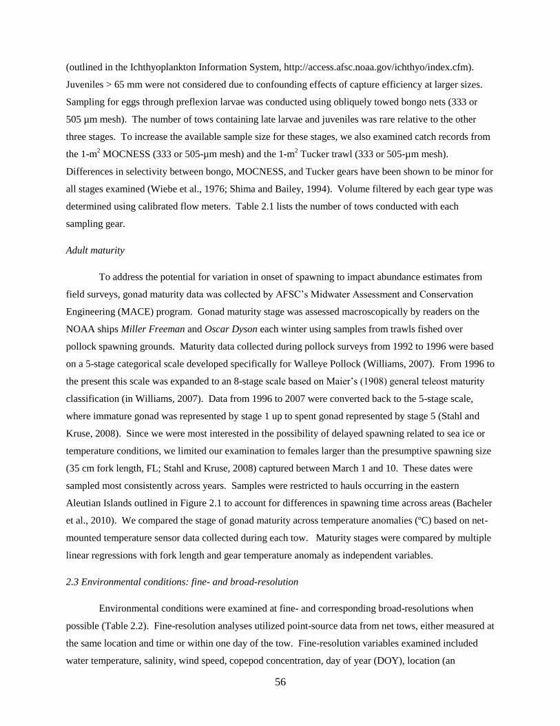
56
(outlined in the Ichthyoplankton Information System, http://access.afsc.noaa.gov/ichthyo/index.cfm).
Juveniles > 65 mm were not considered due to confounding effects of capture efficiency at larger sizes.
Sampling for eggs through preflexion larvae was conducted using obliquely towed bongo nets (333 or
505 µm mesh). The number of tows containing late larvae and juveniles was rare relative to the other
three stages. To increase the available sample size for these stages, we also examined catch records from
the 1-m2 MOCNESS (333 or 505-µm mesh) and the 1-m
2 Tucker trawl (333 or 505-µm mesh).
Differences in selectivity between bongo, MOCNESS, and Tucker gears have been shown to be minor for
all stages examined (Wiebe et al., 1976; Shima and Bailey, 1994). Volume filtered by each gear type was
determined using calibrated flow meters. Table 2.1 lists the number of tows conducted with each
sampling gear.
Adult maturity
To address the potential for variation in onset of spawning to impact abundance estimates from
field surveys, gonad maturity data was collected by AFSC’s Midwater Assessment and Conservation
Engineering (MACE) program. Gonad maturity stage was assessed macroscopically by readers on the
NOAA ships Miller Freeman and Oscar Dyson each winter using samples from trawls fished over
pollock spawning grounds. Maturity data collected during pollock surveys from 1992 to 1996 were based
on a 5-stage categorical scale developed specifically for Walleye Pollock (Williams, 2007). From 1996 to
the present this scale was expanded to an 8-stage scale based on Maier’s (1908) general teleost maturity
classification (in Williams, 2007). Data from 1996 to 2007 were converted back to the 5-stage scale,
where immature gonad was represented by stage 1 up to spent gonad represented by stage 5 (Stahl and
Kruse, 2008). Since we were most interested in the possibility of delayed spawning related to sea ice or
temperature conditions, we limited our examination to females larger than the presumptive spawning size
(35 cm fork length, FL; Stahl and Kruse, 2008) captured between March 1 and 10. These dates were
sampled most consistently across years. Samples were restricted to hauls occurring in the eastern
Aleutian Islands outlined in Figure 2.1 to account for differences in spawning time across areas (Bacheler
et al., 2010). We compared the stage of gonad maturity across temperature anomalies (ºC) based on net-
mounted temperature sensor data collected during each tow. Maturity stages were compared by multiple
linear regressions with fork length and gear temperature anomaly as independent variables.
2.3 Environmental conditions: fine- and broad-resolution
Environmental conditions were examined at fine- and corresponding broad-resolutions when
possible (Table 2.2). Fine-resolution analyses utilized point-source data from net tows, either measured at
the same location and time or within one day of the tow. Fine-resolution variables examined included
water temperature, salinity, wind speed, copepod concentration, day of year (DOY), location (an
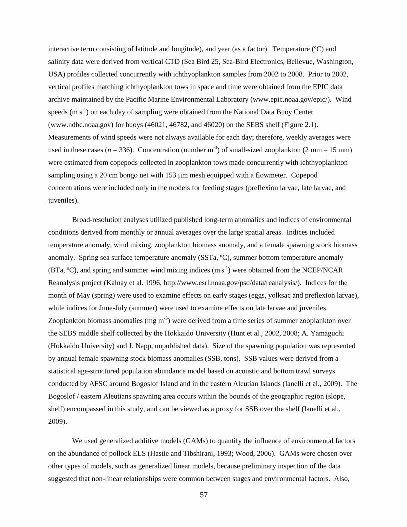
57
interactive term consisting of latitude and longitude), and year (as a factor). Temperature (ºC) and
salinity data were derived from vertical CTD (Sea Bird 25, Sea-Bird Electronics, Bellevue, Washington,
USA) profiles collected concurrently with ichthyoplankton samples from 2002 to 2008. Prior to 2002,
vertical profiles matching ichthyoplankton tows in space and time were obtained from the EPIC data
archive maintained by the Pacific Marine Environmental Laboratory (www.epic.noaa.gov/epic/). Wind
speeds (m s-1
) on each day of sampling were obtained from the National Data Buoy Center
(www.ndbc.noaa.gov) for buoys (46021, 46782, and 46020) on the SEBS shelf (Figure 2.1).
Measurements of wind speeds were not always available for each day; therefore, weekly averages were
used in these cases (n = 336). Concentration (number m-3
) of small-sized zooplankton (2 mm – 15 mm)
were estimated from copepods collected in zooplankton tows made concurrently with ichthyoplankton
sampling using a 20 cm bongo net with 153 µm mesh equipped with a flowmeter. Copepod
concentrations were included only in the models for feeding stages (preflexion larvae, late larvae, and
juveniles).
Broad-resolution analyses utilized published long-term anomalies and indices of environmental
conditions derived from monthly or annual averages over the large spatial areas. Indices included
temperature anomaly, wind mixing, zooplankton biomass anomaly, and a female spawning stock biomass
anomaly. Spring sea surface temperature anomaly (SSTa, ºC), summer bottom temperature anomaly
(BTa, ºC), and spring and summer wind mixing indices (m s
-1) were obtained from the NCEP/NCAR
Reanalysis project (Kalnay et al. 1996, http://www.esrl.noaa.gov/psd/data/reanalysis/). Indices for the
month of May (spring) were used to examine effects on early stages (eggs, yolksac and preflexion larvae),
while indices for June-July (summer) were used to examine effects on late larvae and juveniles.
Zooplankton biomass anomalies (mg m-3
) were derived from a time series of summer zooplankton over
the SEBS middle shelf collected by the Hokkaido University (Hunt et al., 2002, 2008; A. Yamaguchi
(Hokkaido University) and J. Napp, unpublished data). Size of the spawning population was represented
by annual female spawning stock biomass anomalies (SSB, tons). SSB values were derived from a
statistical age-structured population abundance model based on acoustic and bottom trawl surveys
conducted by AFSC around Bogoslof Island and in the eastern Aleutian Islands (Ianelli et al., 2009). The
Bogoslof / eastern Aleutians spawning area occurs within the bounds of the geographic region (slope,
shelf) encompassed in this study, and can be viewed as a proxy for SSB over the shelf (Ianelli et al.,
2009).
We used generalized additive models (GAMs) to quantify the influence of environmental factors
on the abundance of pollock ELS (Hastie and Tibshirani, 1993; Wood, 2006). GAMs were chosen over
other types of models, such as generalized linear models, because preliminary inspection of the data
suggested that non-linear relationships were common between stages and environmental factors. Also,
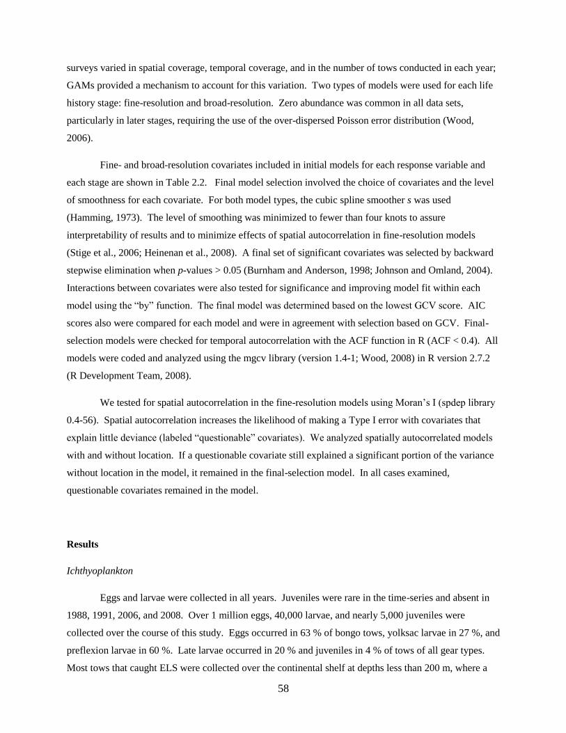
58
surveys varied in spatial coverage, temporal coverage, and in the number of tows conducted in each year;
GAMs provided a mechanism to account for this variation. Two types of models were used for each life
history stage: fine-resolution and broad-resolution. Zero abundance was common in all data sets,
particularly in later stages, requiring the use of the over-dispersed Poisson error distribution (Wood,
2006).
Fine- and broad-resolution covariates included in initial models for each response variable and
each stage are shown in Table 2.2. Final model selection involved the choice of covariates and the level
of smoothness for each covariate. For both model types, the cubic spline smoother s was used
(Hamming, 1973). The level of smoothing was minimized to fewer than four knots to assure
interpretability of results and to minimize effects of spatial autocorrelation in fine-resolution models
(Stige et al., 2006; Heinenan et al., 2008). A final set of significant covariates was selected by backward
stepwise elimination when p-values > 0.05 (Burnham and Anderson, 1998; Johnson and Omland, 2004).
Interactions between covariates were also tested for significance and improving model fit within each
model using the “by” function. The final model was determined based on the lowest GCV score. AIC
scores also were compared for each model and were in agreement with selection based on GCV. Final-
selection models were checked for temporal autocorrelation with the ACF function in R (ACF < 0.4). All
models were coded and analyzed using the mgcv library (version 1.4-1; Wood, 2008) in R version 2.7.2
(R Development Team, 2008).
We tested for spatial autocorrelation in the fine-resolution models using Moran’s I (spdep library
0.4-56). Spatial autocorrelation increases the likelihood of making a Type I error with covariates that
explain little deviance (labeled “questionable” covariates). We analyzed spatially autocorrelated models
with and without location. If a questionable covariate still explained a significant portion of the variance
without location in the model, it remained in the final-selection model. In all cases examined,
questionable covariates remained in the model.
Results
Ichthyoplankton
Eggs and larvae were collected in all years. Juveniles were rare in the time-series and absent in
1988, 1991, 2006, and 2008. Over 1 million eggs, 40,000 larvae, and nearly 5,000 juveniles were
collected over the course of this study. Eggs occurred in 63 % of bongo tows, yolksac larvae in 27 %, and
preflexion larvae in 60 %. Late larvae occurred in 20 % and juveniles in 4 % of tows of all gear types.
Most tows that caught ELS were collected over the continental shelf at depths less than 200 m, where a
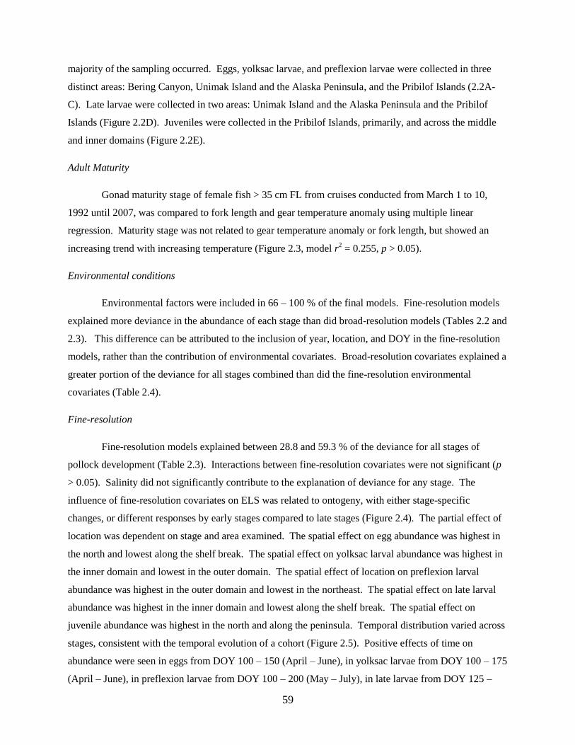
59
majority of the sampling occurred. Eggs, yolksac larvae, and preflexion larvae were collected in three
distinct areas: Bering Canyon, Unimak Island and the Alaska Peninsula, and the Pribilof Islands (2.2A-
C). Late larvae were collected in two areas: Unimak Island and the Alaska Peninsula and the Pribilof
Islands (Figure 2.2D). Juveniles were collected in the Pribilof Islands, primarily, and across the middle
and inner domains (Figure 2.2E).
Adult Maturity
Gonad maturity stage of female fish > 35 cm FL from cruises conducted from March 1 to 10,
1992 until 2007, was compared to fork length and gear temperature anomaly using multiple linear
regression. Maturity stage was not related to gear temperature anomaly or fork length, but showed an
increasing trend with increasing temperature (Figure 2.3, model r2 = 0.255, p > 0.05).
Environmental conditions
Environmental factors were included in 66 – 100 % of the final models. Fine-resolution models
explained more deviance in the abundance of each stage than did broad-resolution models (Tables 2.2 and
2.3). This difference can be attributed to the inclusion of year, location, and DOY in the fine-resolution
models, rather than the contribution of environmental covariates. Broad-resolution covariates explained a
greater portion of the deviance for all stages combined than did the fine-resolution environmental
covariates (Table 2.4).
Fine-resolution
Fine-resolution models explained between 28.8 and 59.3 % of the deviance for all stages of
pollock development (Table 2.3). Interactions between fine-resolution covariates were not significant (p
> 0.05). Salinity did not significantly contribute to the explanation of deviance for any stage. The
influence of fine-resolution covariates on ELS was related to ontogeny, with either stage-specific
changes, or different responses by early stages compared to late stages (Figure 2.4). The partial effect of
location was dependent on stage and area examined. The spatial effect on egg abundance was highest in
the north and lowest along the shelf break. The spatial effect on yolksac larval abundance was highest in
the inner domain and lowest in the outer domain. The spatial effect of location on preflexion larval
abundance was highest in the outer domain and lowest in the northeast. The spatial effect on late larval
abundance was highest in the inner domain and lowest along the shelf break. The spatial effect on
juvenile abundance was highest in the north and along the peninsula. Temporal distribution varied across
stages, consistent with the temporal evolution of a cohort (Figure 2.5). Positive effects of time on
abundance were seen in eggs from DOY 100 – 150 (April – June), in yolksac larvae from DOY 100 – 175
(April – June), in preflexion larvae from DOY 100 – 200 (May – July), in late larvae from DOY 125 –
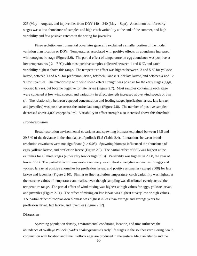
60
225 (May – August), and in juveniles from DOY 140 – 240 (May – Sept). A common trait for early
stages was a low abundance of samples and high catch variability at the end of the summer, and high
variability and few positive catches in the spring for juveniles.
Fine-resolution environmental covariates generally explained a smaller portion of the model
variation than location or DOY. Temperatures associated with positive effects on abundance increased
with ontogenetic stage (Figure 2.6). The partial effect of temperature on egg abundance was positive at
low temperatures (-2 – 7 ºC) with most positive samples collected between 1 and 6 ºC, and catch
variability highest above this range. The temperature effect was highest between -2 and 5 ºC for yolksac
larvae, between 1 and 6 ºC for preflexion larvae, between 3 and 8 ºC for late larvae, and between 4 and 12
ºC for juveniles. The relationship with wind speed effect strength was positive for the early stages (eggs,
yolksac larvae), but became negative for late larvae (Figure 2.7). Most samples containing each stage
were collected at low wind speeds, and variability in effect strength increased above wind speeds of 8 m
s-1
. The relationship between copepod concentration and feeding stages (preflexion larvae, late larvae,
and juveniles) was positive across the entire data range (Figure 2.8). The number of positive samples
decreased above 4,000 copepods / m3. Variability in effect strength also increased above this threshold.
Broad-resolution
Broad-resolution environmental covariates and spawning biomass explained between 14.5 and
29.8 % of the deviance in the abundance of pollock ELS (Table 2.4). Interactions between broad-
resolution covariates were not significant (p > 0.05). Spawning biomass influenced the abundance of
eggs, yolksac larvae, and preflexion larvae (Figure 2.9). The partial effect of SSB was highest at the
extremes for all three stages (either very low or high SSB). Variability was highest in 2008, the year of
lowest SSB. The partial effect of temperature anomaly was highest at negative anomalies for eggs and
yolksac larvae, at positive anomalies for preflexion larvae, and positive anomalies (except 2008) for late
larvae and juveniles (Figure 2.10). Similar to fine-resolution temperature, catch variability was highest at
the extreme values of temperature anomalies, even though sampling was distributed evenly across the
temperature range. The partial effect of wind mixing was highest at high values for eggs, yolksac larvae,
and juveniles (Figure 2.11). The effect of mixing on late larvae was highest at very low or high values.
The partial effect of zooplankton biomass was highest in less than average and average years for
preflexion larvae, late larvae, and juveniles (Figure 2.12).
Discussion
Spawning population density, environmental conditions, location, and time influence the
abundance of Walleye Pollock (Gadus chalcogrammus) early life stages in the southeastern Bering Sea in
conjunction with location and time. Pollock eggs are produced in the eastern Aleutian Islands and the
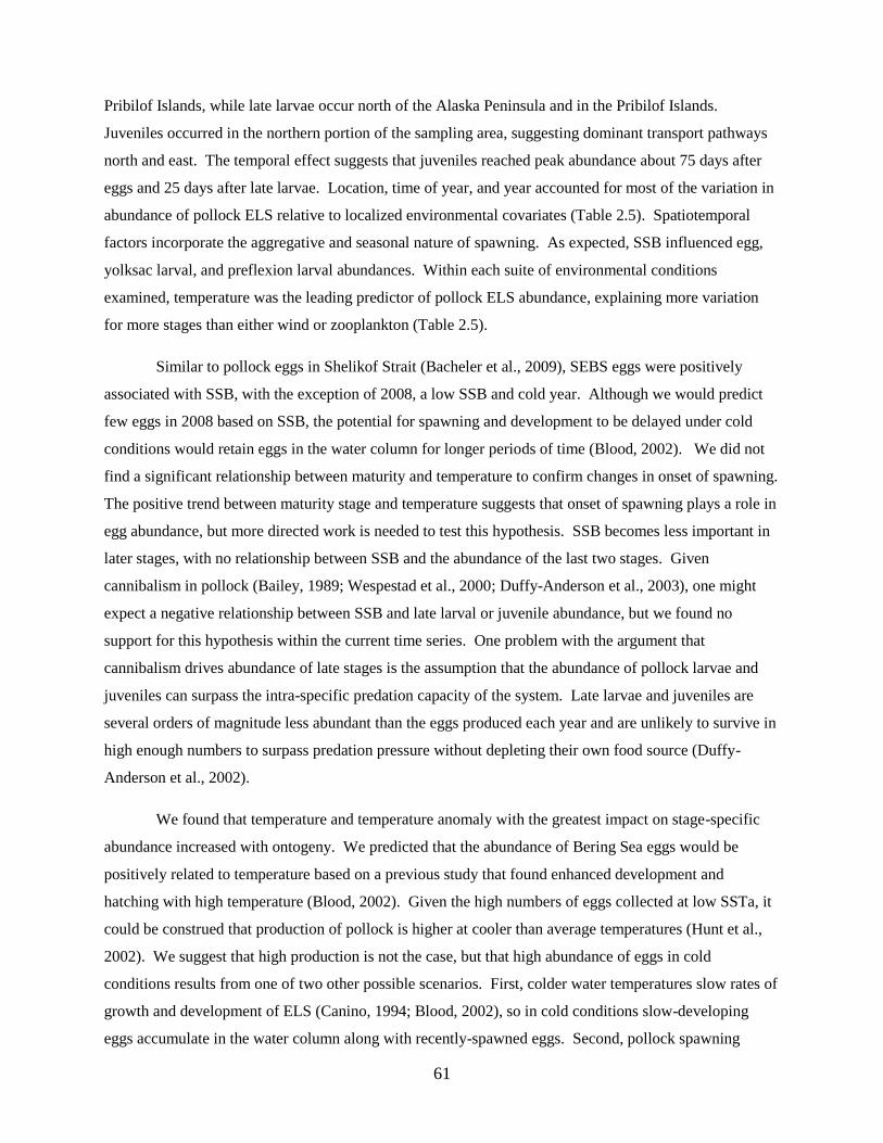
61
Pribilof Islands, while late larvae occur north of the Alaska Peninsula and in the Pribilof Islands.
Juveniles occurred in the northern portion of the sampling area, suggesting dominant transport pathways
north and east. The temporal effect suggests that juveniles reached peak abundance about 75 days after
eggs and 25 days after late larvae. Location, time of year, and year accounted for most of the variation in
abundance of pollock ELS relative to localized environmental covariates (Table 2.5). Spatiotemporal
factors incorporate the aggregative and seasonal nature of spawning. As expected, SSB influenced egg,
yolksac larval, and preflexion larval abundances. Within each suite of environmental conditions
examined, temperature was the leading predictor of pollock ELS abundance, explaining more variation
for more stages than either wind or zooplankton (Table 2.5).
Similar to pollock eggs in Shelikof Strait (Bacheler et al., 2009), SEBS eggs were positively
associated with SSB, with the exception of 2008, a low SSB and cold year. Although we would predict
few eggs in 2008 based on SSB, the potential for spawning and development to be delayed under cold
conditions would retain eggs in the water column for longer periods of time (Blood, 2002). We did not
find a significant relationship between maturity and temperature to confirm changes in onset of spawning.
The positive trend between maturity stage and temperature suggests that onset of spawning plays a role in
egg abundance, but more directed work is needed to test this hypothesis. SSB becomes less important in
later stages, with no relationship between SSB and the abundance of the last two stages. Given
cannibalism in pollock (Bailey, 1989; Wespestad et al., 2000; Duffy-Anderson et al., 2003), one might
expect a negative relationship between SSB and late larval or juvenile abundance, but we found no
support for this hypothesis within the current time series. One problem with the argument that
cannibalism drives abundance of late stages is the assumption that the abundance of pollock larvae and
juveniles can surpass the intra-specific predation capacity of the system. Late larvae and juveniles are
several orders of magnitude less abundant than the eggs produced each year and are unlikely to survive in
high enough numbers to surpass predation pressure without depleting their own food source (Duffy-
Anderson et al., 2002).
We found that temperature and temperature anomaly with the greatest impact on stage-specific
abundance increased with ontogeny. We predicted that the abundance of Bering Sea eggs would be
positively related to temperature based on a previous study that found enhanced development and
hatching with high temperature (Blood, 2002). Given the high numbers of eggs collected at low SSTa, it
could be construed that production of pollock is higher at cooler than average temperatures (Hunt et al.,
2002). We suggest that high production is not the case, but that high abundance of eggs in cold
conditions results from one of two other possible scenarios. First, colder water temperatures slow rates of
growth and development of ELS (Canino, 1994; Blood, 2002), so in cold conditions slow-developing
eggs accumulate in the water column along with recently-spawned eggs. Second, pollock spawning
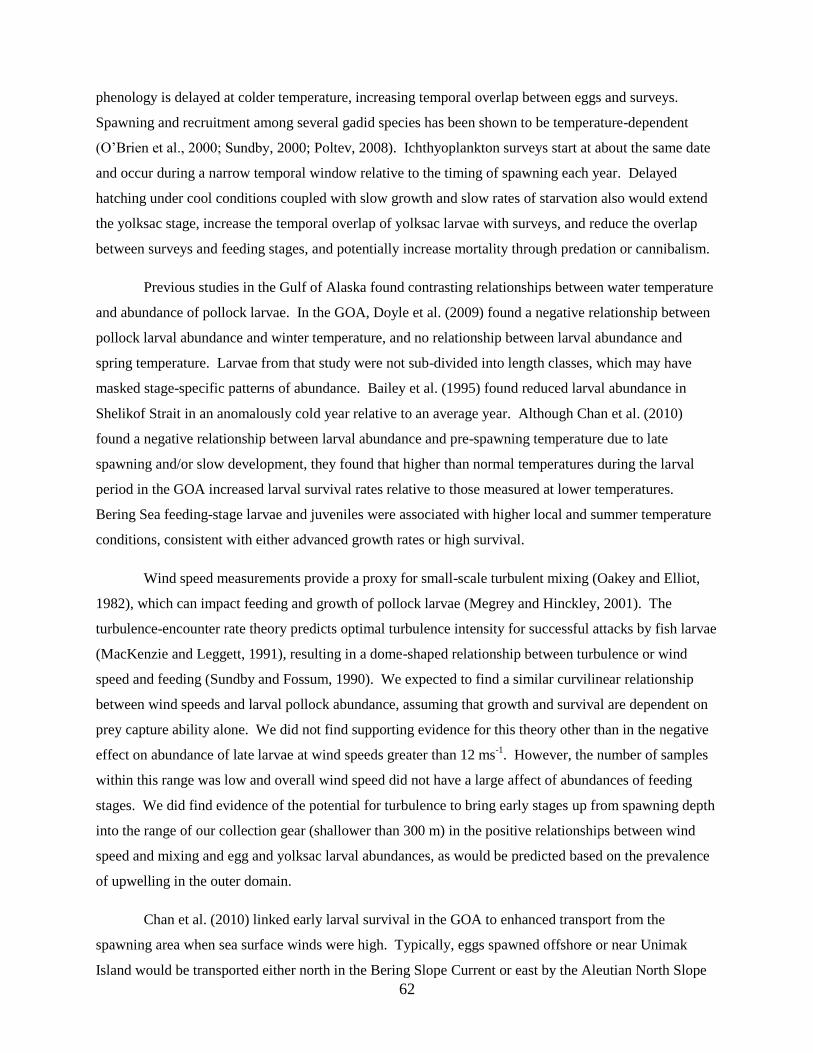
62
phenology is delayed at colder temperature, increasing temporal overlap between eggs and surveys.
Spawning and recruitment among several gadid species has been shown to be temperature-dependent
(O’Brien et al., 2000; Sundby, 2000; Poltev, 2008). Ichthyoplankton surveys start at about the same date
and occur during a narrow temporal window relative to the timing of spawning each year. Delayed
hatching under cool conditions coupled with slow growth and slow rates of starvation also would extend
the yolksac stage, increase the temporal overlap of yolksac larvae with surveys, and reduce the overlap
between surveys and feeding stages, and potentially increase mortality through predation or cannibalism.
Previous studies in the Gulf of Alaska found contrasting relationships between water temperature
and abundance of pollock larvae. In the GOA, Doyle et al. (2009) found a negative relationship between
pollock larval abundance and winter temperature, and no relationship between larval abundance and
spring temperature. Larvae from that study were not sub-divided into length classes, which may have
masked stage-specific patterns of abundance. Bailey et al. (1995) found reduced larval abundance in
Shelikof Strait in an anomalously cold year relative to an average year. Although Chan et al. (2010)
found a negative relationship between larval abundance and pre-spawning temperature due to late
spawning and/or slow development, they found that higher than normal temperatures during the larval
period in the GOA increased larval survival rates relative to those measured at lower temperatures.
Bering Sea feeding-stage larvae and juveniles were associated with higher local and summer temperature
conditions, consistent with either advanced growth rates or high survival.
Wind speed measurements provide a proxy for small-scale turbulent mixing (Oakey and Elliot,
1982), which can impact feeding and growth of pollock larvae (Megrey and Hinckley, 2001). The
turbulence-encounter rate theory predicts optimal turbulence intensity for successful attacks by fish larvae
(MacKenzie and Leggett, 1991), resulting in a dome-shaped relationship between turbulence or wind
speed and feeding (Sundby and Fossum, 1990). We expected to find a similar curvilinear relationship
between wind speeds and larval pollock abundance, assuming that growth and survival are dependent on
prey capture ability alone. We did not find supporting evidence for this theory other than in the negative
effect on abundance of late larvae at wind speeds greater than 12 ms-1
. However, the number of samples
within this range was low and overall wind speed did not have a large affect of abundances of feeding
stages. We did find evidence of the potential for turbulence to bring early stages up from spawning depth
into the range of our collection gear (shallower than 300 m) in the positive relationships between wind
speed and mixing and egg and yolksac larval abundances, as would be predicted based on the prevalence
of upwelling in the outer domain.
Chan et al. (2010) linked early larval survival in the GOA to enhanced transport from the
spawning area when sea surface winds were high. Typically, eggs spawned offshore or near Unimak
Island would be transported either north in the Bering Slope Current or east by the Aleutian North Slope
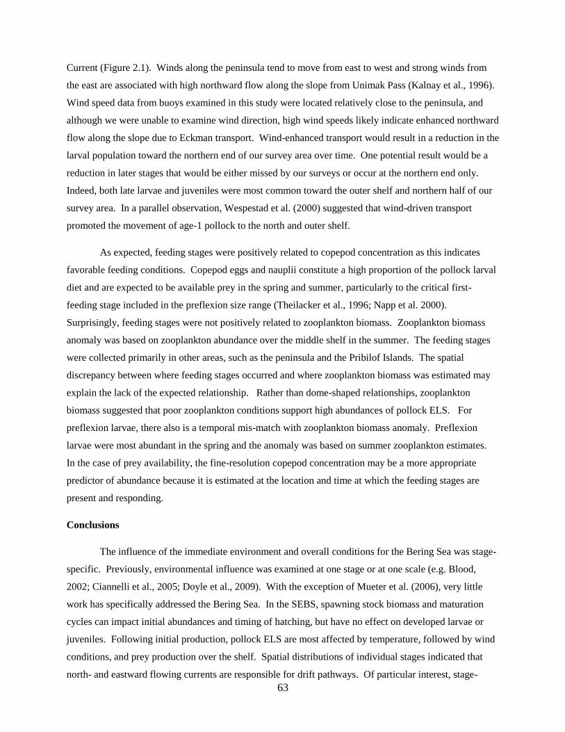
63
Current (Figure 2.1). Winds along the peninsula tend to move from east to west and strong winds from
the east are associated with high northward flow along the slope from Unimak Pass (Kalnay et al., 1996).
Wind speed data from buoys examined in this study were located relatively close to the peninsula, and
although we were unable to examine wind direction, high wind speeds likely indicate enhanced northward
flow along the slope due to Eckman transport. Wind-enhanced transport would result in a reduction in the
larval population toward the northern end of our survey area over time. One potential result would be a
reduction in later stages that would be either missed by our surveys or occur at the northern end only.
Indeed, both late larvae and juveniles were most common toward the outer shelf and northern half of our
survey area. In a parallel observation, Wespestad et al. (2000) suggested that wind-driven transport
promoted the movement of age-1 pollock to the north and outer shelf.
As expected, feeding stages were positively related to copepod concentration as this indicates
favorable feeding conditions. Copepod eggs and nauplii constitute a high proportion of the pollock larval
diet and are expected to be available prey in the spring and summer, particularly to the critical first-
feeding stage included in the preflexion size range (Theilacker et al., 1996; Napp et al. 2000).
Surprisingly, feeding stages were not positively related to zooplankton biomass. Zooplankton biomass
anomaly was based on zooplankton abundance over the middle shelf in the summer. The feeding stages
were collected primarily in other areas, such as the peninsula and the Pribilof Islands. The spatial
discrepancy between where feeding stages occurred and where zooplankton biomass was estimated may
explain the lack of the expected relationship. Rather than dome-shaped relationships, zooplankton
biomass suggested that poor zooplankton conditions support high abundances of pollock ELS. For
preflexion larvae, there also is a temporal mis-match with zooplankton biomass anomaly. Preflexion
larvae were most abundant in the spring and the anomaly was based on summer zooplankton estimates.
In the case of prey availability, the fine-resolution copepod concentration may be a more appropriate
predictor of abundance because it is estimated at the location and time at which the feeding stages are
present and responding.
Conclusions
The influence of the immediate environment and overall conditions for the Bering Sea was stage-
specific. Previously, environmental influence was examined at one stage or at one scale (e.g. Blood,
2002; Ciannelli et al., 2005; Doyle et al., 2009). With the exception of Mueter et al. (2006), very little
work has specifically addressed the Bering Sea. In the SEBS, spawning stock biomass and maturation
cycles can impact initial abundances and timing of hatching, but have no effect on developed larvae or
juveniles. Following initial production, pollock ELS are most affected by temperature, followed by wind
conditions, and prey production over the shelf. Spatial distributions of individual stages indicated that
north- and eastward flowing currents are responsible for drift pathways. Of particular interest, stage-
64
specific changes in abundance occurred at different temperatures, with an oscillation between early stages
at low temperatures and late stages at high temperatures. When available, fine-resolution environmental
data are useful for modeling and predicting responses of individual stages to changing conditions. When
fine-resolution data is unavailable or limited, patterns from broad-resolution indices paralleled those of
their fine-scale counterparts, with the caveats that broad-resolution factors may not have been measured
in similar locations or at similar times in which pollock ELS occur. Our results emphasize the importance
of including ontogeny when predicting responses to environmental change, as ecological constraints
imposed on a given stage do not necessarily act upon other stages in a similar manner.
Acknowledgements
Many thanks to the members of NOAA’s Ecosystems and Fisheries Oceanography Coordinated
Investigations (EcoFOCI) who were involved in the collection and processing of the ichthyoplankton
samples. L. Ciannelli assisted with statistical analyses and interpretation. A. Yamaguchi of the Hokkaido
Univ. Graduate School of Fisheries provided zooplankton data for biomass anomalies. Earlier versions of
this manuscript benefited from comments by Kevin Bailey, Jerry Berger, and three anonymous reviewers.
This research was supported by the BSIERP program of the North Pacific Research Board (NPRB). This
paper is EcoFOCI Contribution No. N753-RAOA-0 to NOAA's North Pacific Climate Regimes and
Ecosystem Productivity research program, BEST-BSIERP Publication No. 35, and NPRB Publication No.
337, and BSIERP publication number 51.
65
Literature Cited
Bacheler, N.M., Bailey, K.M., Ciannelli, L., Bartolino, V., Chan, K.S., 2009. Density-dependent,
landscape, and climate effects on spawning distribution of walleye pollock Theragra
chalcogramma. Mar. Ecol. Prog. Ser. 391, 1-12.
Bacheler, N.M., Ciannelli, L., Bailey, K.M., Duffy-Anderson, J.T., 2010. Spatial and temporal patterns of
walleye pollock spawning in the eastern Bering Sea inferred from egg and larval distributions.
Fish. Oceanogr.19, 107-120.
Bailey, K.M., 1989. Interaction between the vertical distribution of juvenile walleye pollock Theragra
chalcogramma in the eastern Bering Sea and cannibalism. Mar. Ecol. Prog. Ser. 53, 205-213.
Bailey, K.M., Macklin, S.A., 1994. Analysis of patterns in larval Walleye Pollock Theragra
chalcogramma survival and wind mixing events in Shelikof Strait, Gulf of Alaska. Mar. Ecol.
Prog. Ser. 113, 1-12.
Bailey, K.M., Canino, M.F., Napp, J.M., Spring, S.M., Brown, A.L., 1995. Contrasting years of prey
levels, feeding conditions and mortality of larval walleye pollock Theragra chalcogramma in the
western Gulf of Alaska. Mar. Ecol. Prog. Ser. 119, 11-23.
Bakkala, R.G., 1993. Structure and historical changes in the groundfish complex of the eastern Bering
Sea. NOAA Tech. Rep. 114, 91 pp.
Bivand, R.S., Pebesma, E.J., Gómez-Rubio, V., 2008. Applied Spatial Data Analysis with R. New York,
Springer.
Blood, D.M., 2002. Low-temperature incubation of walleye pollock (Theragra chalcogramma) eggs from
the southeastern Bering Sea shelf and Shelikof Strait, Gulf of Alaska. Deep-Sea Res. II 49, 6095–
6108.
Burnham, K.P., Anderson, D.R., 1998. Model Selection and Inference: A Practical Information-
Theoretical Approach. Springer, New York.
Canino, M. 1994. Effects of temperature and food availability on growth and RNA/DNA ratios of
walleye pollock Theragra chalcogramma (Pallas) eggs and larvae. J. Exp. Mar. Biol. Ecol. 17,
1-16.
Chan, K-S., Zhang, T., Bailey, K.M., 2010. Otolith biochronology reveals factors underlying dynamics
of marine fish larvae. Mar. Ecol. Prog. Ser. 412, 1-10.
Ciannelli, L., Chan, K.S., Bailey, K.M., Stenseth, N.C., 2004. Nonadditive effects of the environment on
the survival of a large marine fish population. Ecology 85, 3418-3427.
66
Ciannelli, L., Bailey, K.M., Chan, K.S., Belgrano, A., Stenseth, N.C., 2005. Climate change causing
phase transitions of walleye pollock (Theragra chalcogramma) recruitment dynamics. Proc. R.
Soc. Lond. B Biol. Sci. 272, 1735-1743.
Doyle, M.J., Picquelle, S.J., Mier, K.L., Spillane, M.C., Bond, N.A., 2009. Larval fish abundance and
physical forcing in the Gulf of Alaska, 1981-2003. Prog. Oceanogr. 80, 163-187.
Duffy-Anderson, J.T., Bailey, K., Ciannelli L., 2002. Consequences of a superabundance of larval
walleye pollock Theragra chalcogramma in the Gulf of Alaska in 1981. Mar. Ecol. Prog. Ser.
243, 179-190.
Duffy-Anderson, J.T., Ciannelli, L., Honkalehto, T. Bailey, K.M., Sogard, S.M., Springer, A., Buckley,
T., 2003. Distribution of age-1 and age-2 walleye pollock in the Gulf of Alaska and Eastern
Bering Sea: sources of variation and implications for higher trophic levels. In: Browman, H., A.
Skiftesvik (eds.), The big fish bang: Proceedings from the 26th annual larval fish conference, 381-
394.
Duffy-Anderson, J.T., Bailey, K., Ciannelli L., Cury, P., Belgrano, A., Stenseth N.C., 2005. Phase
transitions in marine fish recruitment processes. Ecological Complexity 2, 205-218.
FAO, 2007. 15 December 2009. Yearbooks of Fisheries Statistics.
[http://www.fao.org/fishery/statistics/en].
Fukuchi, M., 1976. Some aspects of bioenergetics of walleye pollock Theragra chalcogramma (Pallas) at
early life stages. Ph. D. thesis, Univ. of Hokkaido, Hokkaido, Japan.
Hamming, R.W., 1973. Numerical Methods for Scientists and Engineers. McGraw-Hill, New York.
Hastie, T., Tibshirani, R., 1993. Varying-coefficient models. J. R. Stat. Soc. B 55, 757-796.
Heinenän, S., Rönkä, M., von Numers, M., 2008. Modeling the occurrence and abundance of a colonial
species, the arctic tern Sterna paradisaea in the archipelago of SW Finland. Ecography 31, 601-
611.
Hunt, G.L., Stabeno, P.J., Walters, G., Sinclair, E., Brodeur, R.D., Napp, J.M., Bond, N.A., 2002. Climate
change and control of the southeastern Bering Sea pelagic ecosystem. Deep-Sea Res. II 49, 5821-
5853.
67
Hunt, G.L., Stabeno, P.J., Strom, S., Napp, J.M., 2008. Patterns of spatial and temporal variation in the
marine ecosystem of the southeastern Bering Sea, with special reference to the Pribilof Domain.
Deep-Sea Res. II 55, 1919-1944.
Ianelli, J.N., Barbeaux, S., Honkalehto, T., Kotwicki, S., Aydin, K., Williamson, N., 2009. Assessment of
the Walleye Pollock stock in the Eastern Bering Sea. In: Stock assessment and fishery evaluation
report for the groundfish resources of the Bering Sea/Aleutian Islands regions. North Pac. Fish.
Mgmt. Council, Anchorage, AK, section 1, 49-148.
Ichthyoplankton Information System. 23 July 2009. National Oceanic and Atmospheric Administration.
[http://access.afsc.noaa.gov/ichthyo/index.cfm].
Johnson, J.B., Omland, K.S., 2004. Model selection in ecology and evolution. Trends Ecol. Evol. 19, 101-
108.
Kalnay, E., Kanamitsu, M., Kistler, R., Collins, W., Deaven, D., Gandin, L., Iredell, M., Saha, S., White,
G., Woollen, J., Zhu, Y., Leetmaa, A., Reynolds, B., Chelliah, M., Ebisuzaki, W., Higgins, W.,
Janowiak, J., Mo, K., Ropelewski, C., Wang, J., Jenne, R., Joseph, D., 1996. The NCEP/NCAR
40-year reanalysis project. Bull. Am. Meteorological Soc. 77, 437–471.
Logerwell, E., Duffy-Anderson, J.T., Wilson, M.T., McKelvey, D. 2010. The physical and biological
processes resulting in habitat partitioning by two potential competitors, juvenile pollock and
capelin, in the Gulf of Alaska. Fish. Oceanogr. 19, 262-278.
MacKenzie, B.R., Leggett, W.C., 1991. Quantifying the contribution of small-scale turbulence to the
encounter rates between larval fish and their zooplankton prey: Effects of wind and tide. Mar.
Ecol. Prog. Ser. 73, 149-160.
Matarese, A.C., Blood, D.M., Picquelle, S.J., Benson, J.L., 2003. Atlas of abundance and distribution
patterns of ichthyoplankton from the northeast Pacific Ocean and Bering Sea ecosystems based
on research conducted by the Alaska Fisheries Science Center (1972-1996). NOAA Prof. Pap.
NMFS No. 1, NOAA, Seattle, WA.
Megrey, B.A., Hinckley, S., 2001. Effect of turbulence on feeding of larval fishes: a sensitivity analysis
using an individual-based model. ICES J. Mar. Sci. 58, 1015-1029.
Mueter, F.J., Ladd, C., Palmer, M.C., Norcross, B.L., 2006. Bottom-up and top-down controls of walleye
pollock (Theragra chalcogramma) on the eastern Bering Sea shelf. Prog. Oceanogr. 68, 152-183.
Oakey, N.S., Elliott, J.A., 1982. Dissipation within the surface mixed layer. J. Phys. Oceanogr. 12, 171-
185.
68
O’Brien, C.M., Fox, C.J., Planque, B., Casey, J., 2000. Climate variability and North Sea cod. Nature
404, 142.
Olla, B.L. Davis, M.W., Ryer, C.H., Sogard, S.M., 1996. Behavioural determinants of distribution and
survival in early stages of walleye pollock, Theragra chalcogramma: a synthesis of experimental
studies. Fish. Oceanogr. 5, 167-178.
Poltev, Y.N., 2008. Some issues related to reproduction of Pacific cod Gadus macrocephalus in waters of
the eastern coast of the North Kuril Islands and the southern extremity of Kamchatka. J. Ichthyol.
48: 345-355.
Porter, S.M., Ciannelli, L., Hillgruber, N., Bailey, K.M., Chan, K-S., Canino, M.F., Haldorson, L.J., 2005.
Environmental factors influencing larval walleye pollock Theragra chalcogramma feeding in
Alaskan waters. Mar. Ecol. Prog. Ser. 302, 207-217.
Potts, J.M., Elith, J., 2006. Comparing species abundance models. Ecol. Modelling 199, 153-163.
R Development Core Team, 2008. R: a language and environment for statistical computing. R Foundation
for Statistical Computing, Vienna.
Shima, M., Bailey, K.M., 1994. Comparative analysis of ichthyoplankton sampling gear for early life
stages of walleye pollock (Theragra chalcogramma). Fish. Oceanogr. 3, 50-59.
Stige, L.C., Ottersen, G., Brander, K., Chan, K.S., Stenseth, N.C., 2006. Cod and climate: effect of the
North Atlantic Oscillation on recruitment in the North Atlantic. Mar. Ecol. Prog. Ser. 325, 227–
241.
Stahl, J.P., Kruse, G.H., 2008. Spatial and temporal variability in size at maturity of walleye pollock in
the eastern Bering Sea. Trans. Am. Fish. Soc. 137, 1543-1557.
Sundby, S., 2000. Recruitment of Atlantic cod stocks in relation to temperature and advection of copepod
populations. Sarsia 85, 277–298.
Sundby, S., Fossum, P., 1990. Feeding conditions of Arcto-Norwegian cod larvae compared with the
Rothschild–Osborn theory on small-scale turbulence and plankton contact rates. J. Plankton Res.
12, 1153–1162.
Theilacker, G.H., Bailey, K.M., Canino, M.F., Porter, S.M., 1996. Variations in larval walleye pollock
feeding and condition: a synthesis. Fish. Oceanogr. 5, 112-123.
69
Walline, P.D., 1985. Growth of larval Walleye Pollock related to domains within the SE Bering Sea. Mar.
Ecol. Prog. Ser. 21, 197-203.
Wespestad, V. G., Fritz, L. W., Ingraham, W. J., Megrey, B. A., 2000. On relationships between
cannibalism, climate variability, physical transport, and recruitment success of Bering Sea
walleye pollock (Theragra chalcogramma). ICES J. Mar. Sci. 57, 268–274.
Wiebe, P.H., Burt, K.H., Boyd, S.H., Morton, A.W., 1976. A multiple opening/closing net and
environmental sensing system for sampling zooplankton. J. Mar. Res. 34, 313-326.
Williams, K., 2007. Evaluation of the macroscopic staging method for determining maturity of female
Walleye Pollock Theragra chalcogramma in Shelikof Strait, Alaska. Alaska Fish. Res. Bull. 12,
252-263
Wilson, M.T., 2009. Ecology of small neritic fishes in the western Gulf of Alaska. I. Geographic
distribution in relation to prey abundance and the physical environment. Mar. Ecol. Prog. Ser.
392, 223-237.
Wood, S.N., 2006. Generalized Additive Models: An Introduction with R. Chapman & Hall/CRC, Boca
Raton, FL.
Wood, S.N., 2008. Fast stable direct fitting and smoothness selection for generalized additive models. J.
R. Stat. Soc. Ser. B Stat. Method. 70, 495-518.
Zarauz, L., Irigoien, X., Urtizberea, A., Gonzalez, M., 2007. Mapping plankton distribution in the Bay of
Biscay during three consecutive spring surveys. Mar. Ecol. Prog. Ser. 345, 27-39.
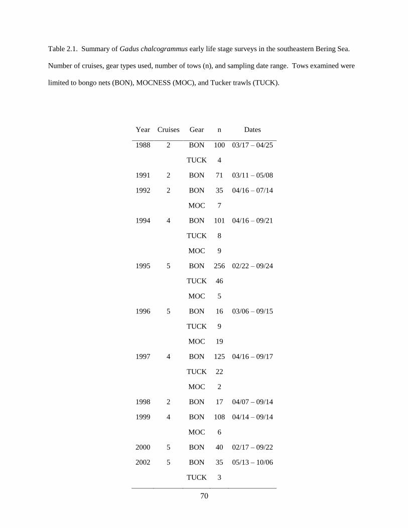
70
Table 2.1. Summary of Gadus chalcogrammus early life stage surveys in the southeastern Bering Sea.
Number of cruises, gear types used, number of tows (n), and sampling date range. Tows examined were
limited to bongo nets (BON), MOCNESS (MOC), and Tucker trawls (TUCK).
Year Cruises Gear n Dates
1988 2 BON 100 03/17 – 04/25
TUCK 4
1991 2 BON 71 03/11 – 05/08
1992 2 BON 35 04/16 – 07/14
MOC 7
1994 4 BON 101 04/16 – 09/21
TUCK 8
MOC 9
1995 5 BON 256 02/22 – 09/24
TUCK 46
MOC 5
1996 5 BON 16 03/06 – 09/15
TUCK 9
MOC 19
1997 4 BON 125 04/16 – 09/17
TUCK 22
MOC 2
1998 2 BON 17 04/07 – 09/14
1999 4 BON 108 04/14 – 09/14
MOC 6
2000 5 BON 40 02/17 – 09/22
2002 5 BON 35 05/13 – 10/06
TUCK 3
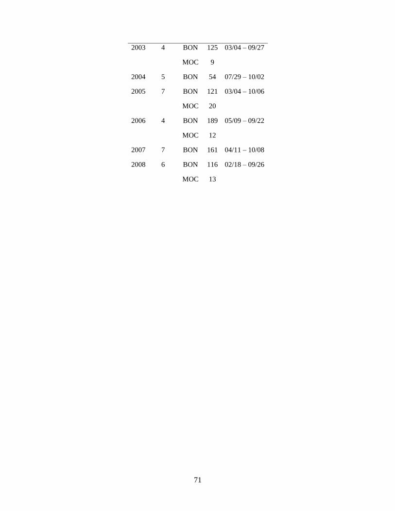
71
2003 4 BON 125 03/04 – 09/27
MOC 9
2004 5 BON 54 07/29 – 10/02
2005 7 BON 121 03/04 – 10/06
MOC 20
2006 4 BON 189 05/09 – 09/22
MOC 12
2007 7 BON 161 04/11 – 10/08
2008 6 BON 116 02/18 – 09/26
MOC 13
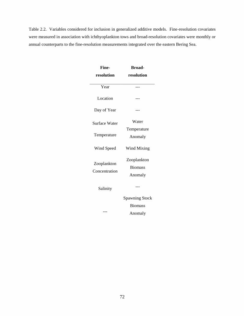
72
Table 2.2. Variables considered for inclusion in generalized additive models. Fine-resolution covariates
were measured in association with ichthyoplankton tows and broad-resolution covariates were monthly or
annual counterparts to the fine-resolution measurements integrated over the eastern Bering Sea.
Fine-
resolution
Broad-
resolution
Year ---
Location ---
Day of Year ---
Surface Water
Temperature
Water
Temperature
Anomaly
Wind Speed Wind Mixing
Zooplankton
Concentration
Zooplankton
Biomass
Anomaly
Salinity ---
---
Spawning Stock
Biomass
Anomaly
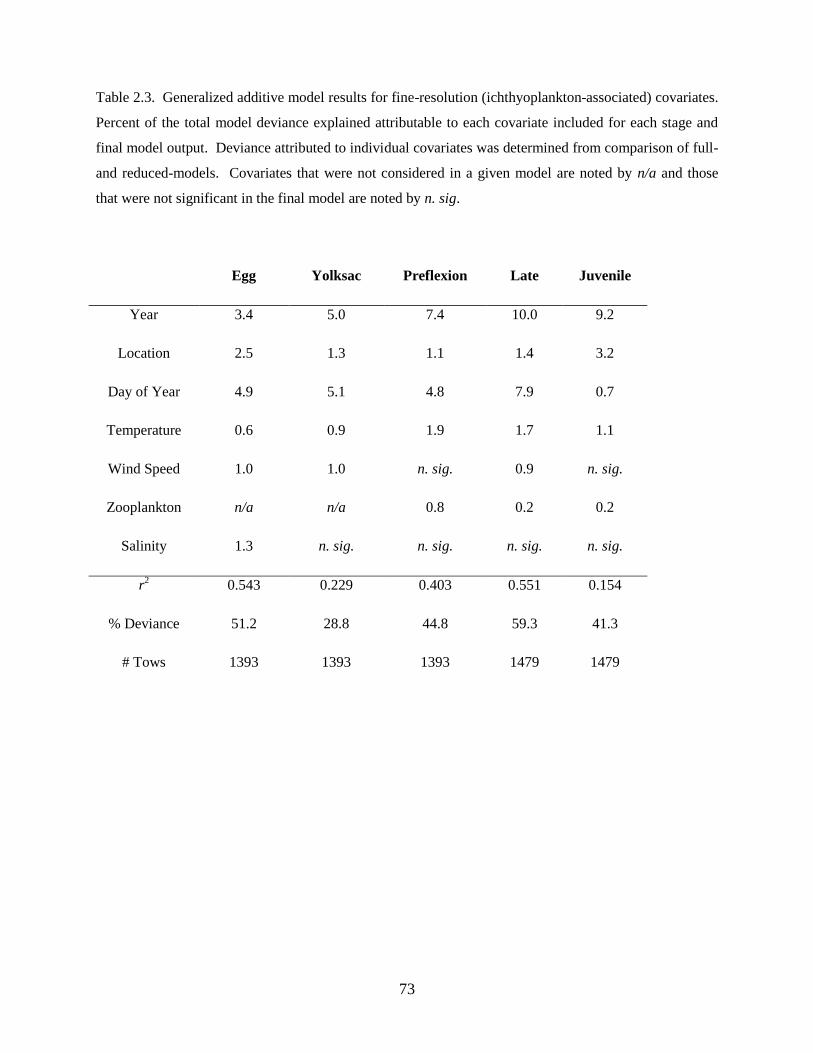
73
Table 2.3. Generalized additive model results for fine-resolution (ichthyoplankton-associated) covariates.
Percent of the total model deviance explained attributable to each covariate included for each stage and
final model output. Deviance attributed to individual covariates was determined from comparison of full-
and reduced-models. Covariates that were not considered in a given model are noted by n/a and those
that were not significant in the final model are noted by n. sig.
Egg Yolksac Preflexion Late Juvenile
Year 3.4 5.0 7.4 10.0 9.2
Location 2.5 1.3 1.1 1.4 3.2
Day of Year 4.9 5.1 4.8 7.9 0.7
Temperature 0.6 0.9 1.9 1.7 1.1
Wind Speed 1.0 1.0 n. sig. 0.9 n. sig.
Zooplankton n/a n/a 0.8 0.2 0.2
Salinity 1.3 n. sig. n. sig. n. sig. n. sig.
r2 0.543 0.229 0.403 0.551 0.154
% Deviance 51.2 28.8 44.8 59.3 41.3
# Tows 1393 1393 1393 1479 1479
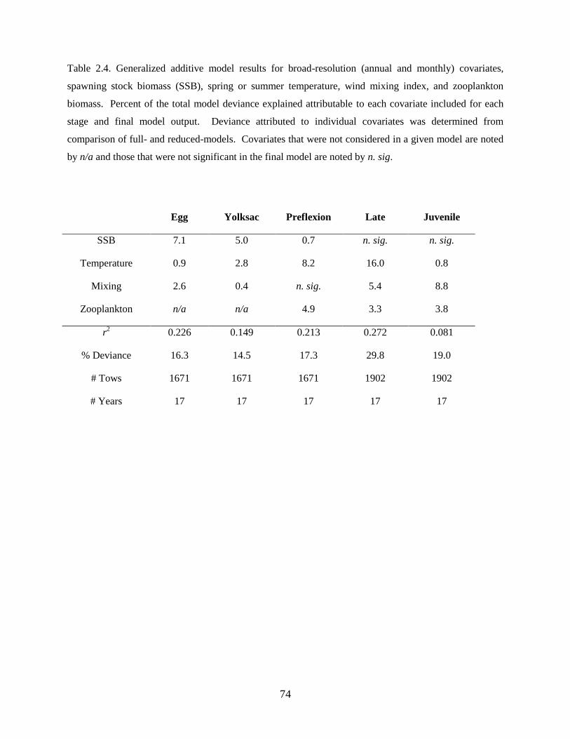
74
Table 2.4. Generalized additive model results for broad-resolution (annual and monthly) covariates,
spawning stock biomass (SSB), spring or summer temperature, wind mixing index, and zooplankton
biomass. Percent of the total model deviance explained attributable to each covariate included for each
stage and final model output. Deviance attributed to individual covariates was determined from
comparison of full- and reduced-models. Covariates that were not considered in a given model are noted
by n/a and those that were not significant in the final model are noted by n. sig.
Egg Yolksac Preflexion Late Juvenile
SSB 7.1 5.0 0.7 n. sig. n. sig.
Temperature 0.9 2.8 8.2 16.0 0.8
Mixing 2.6 0.4 n. sig. 5.4 8.8
Zooplankton n/a n/a 4.9 3.3 3.8
r2 0.226 0.149 0.213 0.272 0.081
% Deviance 16.3 14.5 17.3 29.8 19.0
# Tows 1671 1671 1671 1902 1902
# Years 17 17 17 17 17
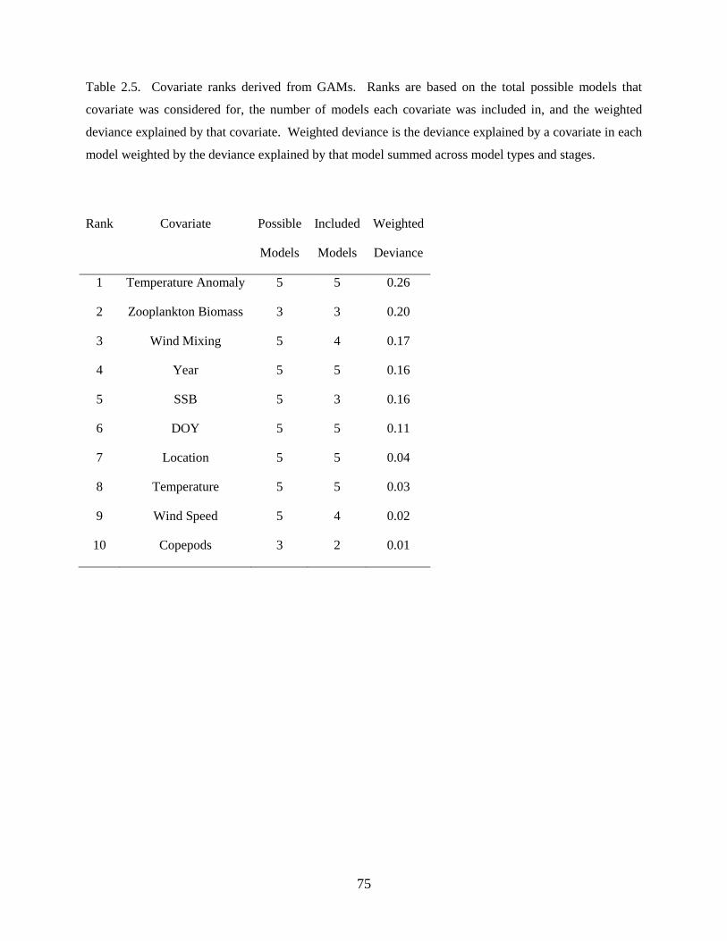
75
Table 2.5. Covariate ranks derived from GAMs. Ranks are based on the total possible models that
covariate was considered for, the number of models each covariate was included in, and the weighted
deviance explained by that covariate. Weighted deviance is the deviance explained by a covariate in each
model weighted by the deviance explained by that model summed across model types and stages.
Rank Covariate Possible
Models
Included
Models
Weighted
Deviance
1 Temperature Anomaly 5 5 0.26
2 Zooplankton Biomass 3 3 0.20
3 Wind Mixing 5 4 0.17
4 Year 5 5 0.16
5 SSB 5 3 0.16
6 DOY 5 5 0.11
7 Location 5 5 0.04
8 Temperature 5 5 0.03
9 Wind Speed 5 4 0.02
10 Copepods 3 2 0.01
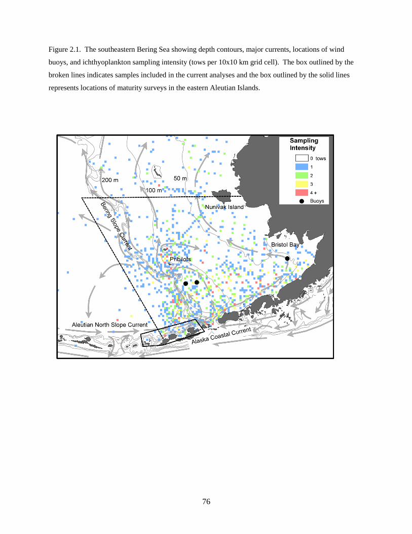
76
Figure 2.1. The southeastern Bering Sea showing depth contours, major currents, locations of wind
buoys, and ichthyoplankton sampling intensity (tows per 10x10 km grid cell). The box outlined by the
broken lines indicates samples included in the current analyses and the box outlined by the solid lines
represents locations of maturity surveys in the eastern Aleutian Islands.

77
Figure 2.2. Walleye Pollock early life stages in the southeastern Bering Sea. Relative abundances of A)
eggs, B) yolksac larvae, C) preflexion larvae, D) late larvae, and E) juveniles. The size of the bubbles is
scaled to the largest catch within each stage.
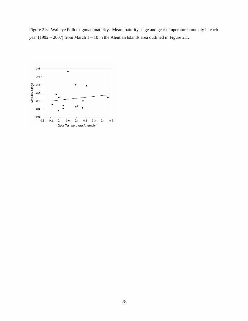
78
Figure 2.3. Walleye Pollock gonad maturity. Mean maturity stage and gear temperature anomaly in each
year (1992 – 2007) from March 1 – 10 in the Aleutian Islands area outlined in Figure 2.1.
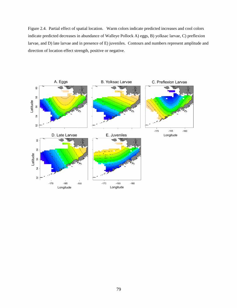
79
Figure 2.4. Partial effect of spatial location. Warm colors indicate predicted increases and cool colors
indicate predicted decreases in abundance of Walleye Pollock A) eggs, B) yolksac larvae, C) preflexion
larvae, and D) late larvae and in presence of E) juveniles. Contours and numbers represent amplitude and
direction of location effect strength, positive or negative.
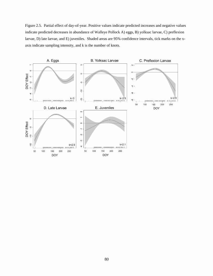
80
Figure 2.5. Partial effect of day-of-year. Positive values indicate predicted increases and negative values
indicate predicted decreases in abundance of Walleye Pollock A) eggs, B) yolksac larvae, C) preflexion
larvae, D) late larvae, and E) juveniles. Shaded areas are 95% confidence intervals, tick marks on the x-
axis indicate sampling intensity, and k is the number of knots.
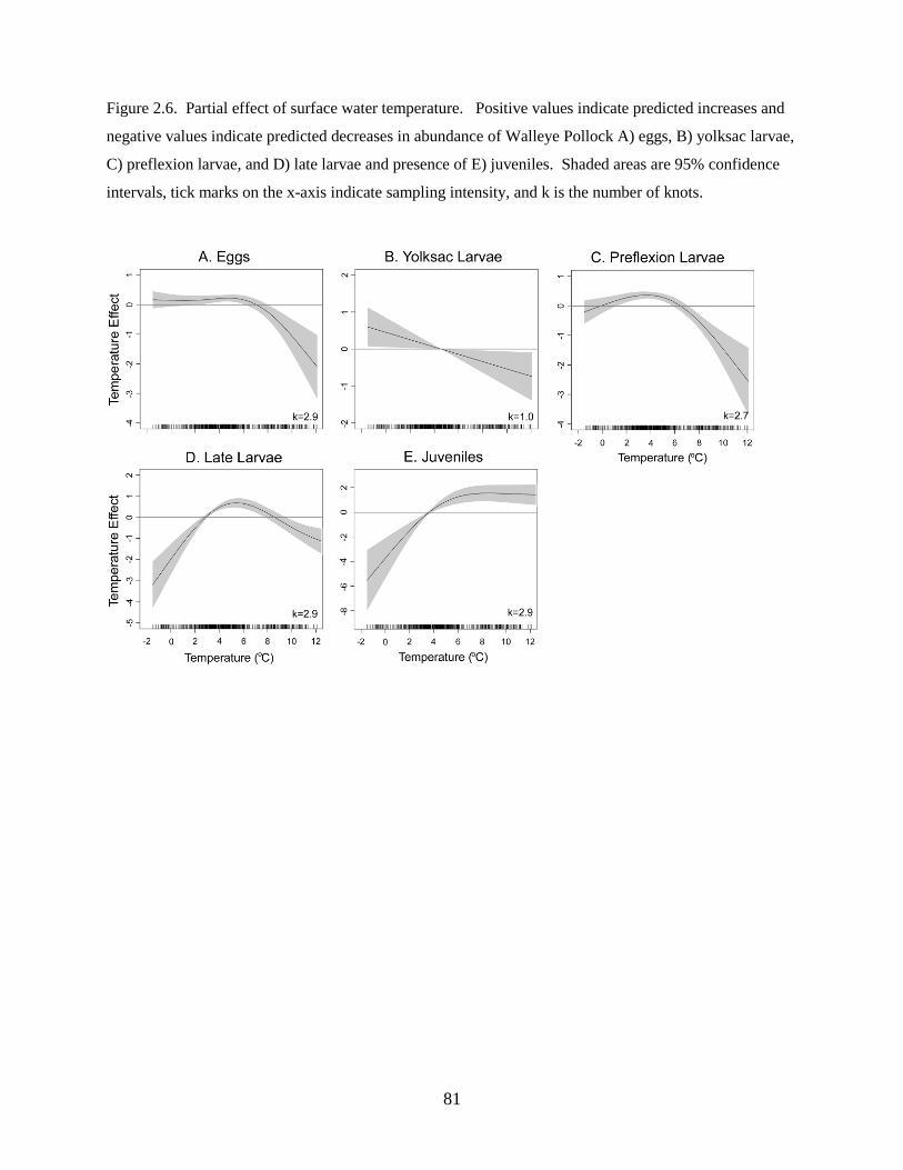
81
Figure 2.6. Partial effect of surface water temperature. Positive values indicate predicted increases and
negative values indicate predicted decreases in abundance of Walleye Pollock A) eggs, B) yolksac larvae,
C) preflexion larvae, and D) late larvae and presence of E) juveniles. Shaded areas are 95% confidence
intervals, tick marks on the x-axis indicate sampling intensity, and k is the number of knots.
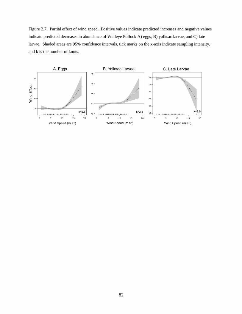
82
Figure 2.7. Partial effect of wind speed. Positive values indicate predicted increases and negative values
indicate predicted decreases in abundance of Walleye Pollock A) eggs, B) yolksac larvae, and C) late
larvae. Shaded areas are 95% confidence intervals, tick marks on the x-axis indicate sampling intensity,
and k is the number of knots.
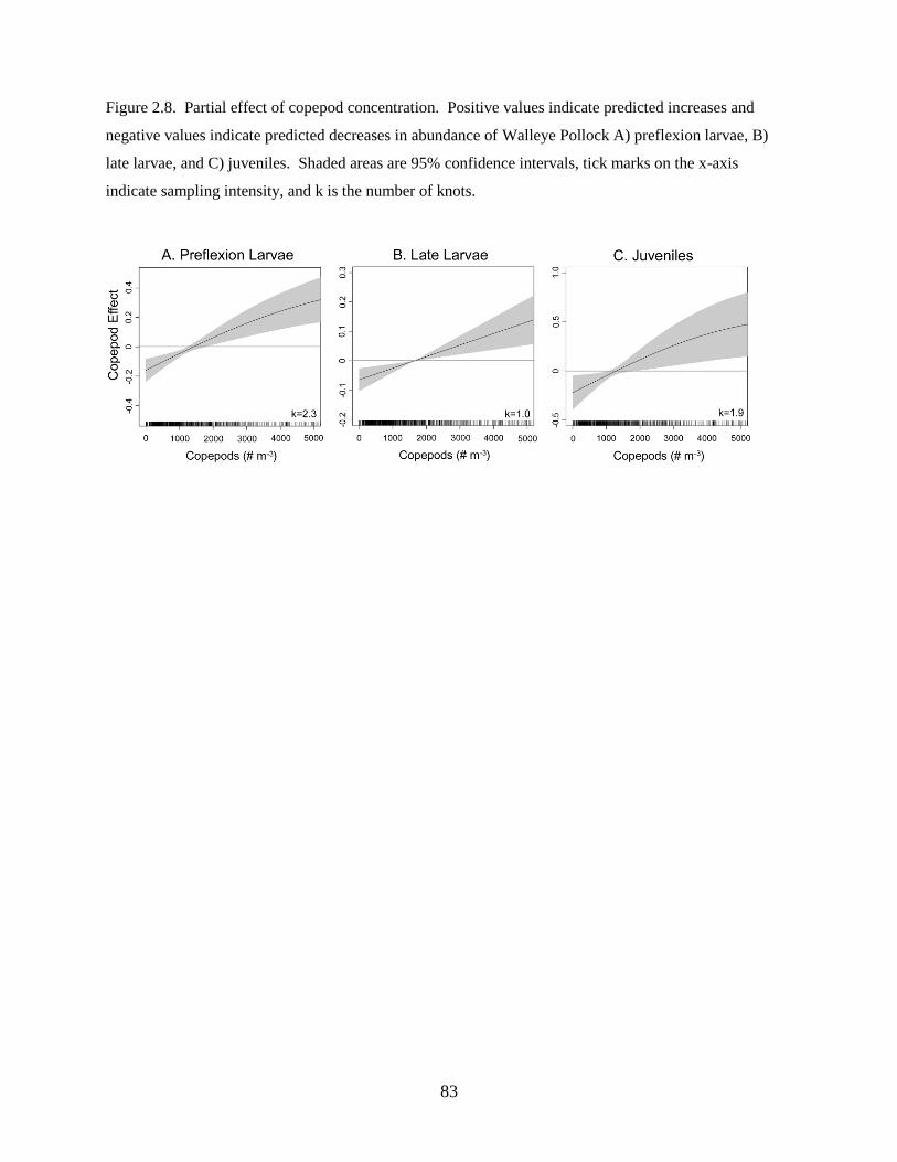
83
Figure 2.8. Partial effect of copepod concentration. Positive values indicate predicted increases and
negative values indicate predicted decreases in abundance of Walleye Pollock A) preflexion larvae, B)
late larvae, and C) juveniles. Shaded areas are 95% confidence intervals, tick marks on the x-axis
indicate sampling intensity, and k is the number of knots.
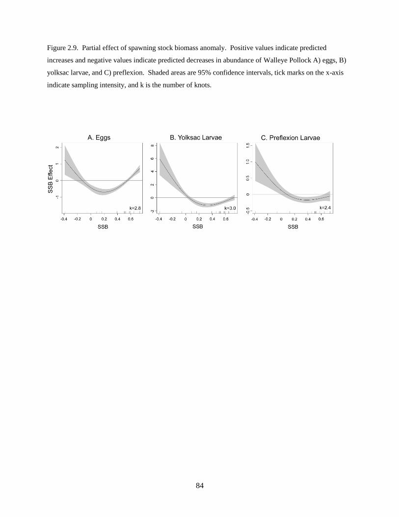
84
Figure 2.9. Partial effect of spawning stock biomass anomaly. Positive values indicate predicted
increases and negative values indicate predicted decreases in abundance of Walleye Pollock A) eggs, B)
yolksac larvae, and C) preflexion. Shaded areas are 95% confidence intervals, tick marks on the x-axis
indicate sampling intensity, and k is the number of knots.
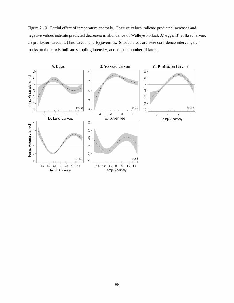
85
Figure 2.10. Partial effect of temperature anomaly. Positive values indicate predicted increases and
negative values indicate predicted decreases in abundance of Walleye Pollock A) eggs, B) yolksac larvae,
C) preflexion larvae, D) late larvae, and E) juveniles. Shaded areas are 95% confidence intervals, tick
marks on the x-axis indicate sampling intensity, and k is the number of knots.
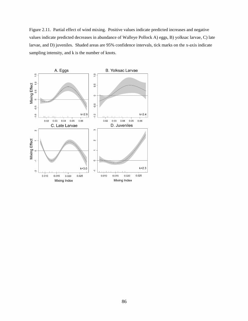
86
Figure 2.11. Partial effect of wind mixing. Positive values indicate predicted increases and negative
values indicate predicted decreases in abundance of Walleye Pollock A) eggs, B) yolksac larvae, C) late
larvae, and D) juveniles. Shaded areas are 95% confidence intervals, tick marks on the x-axis indicate
sampling intensity, and k is the number of knots.
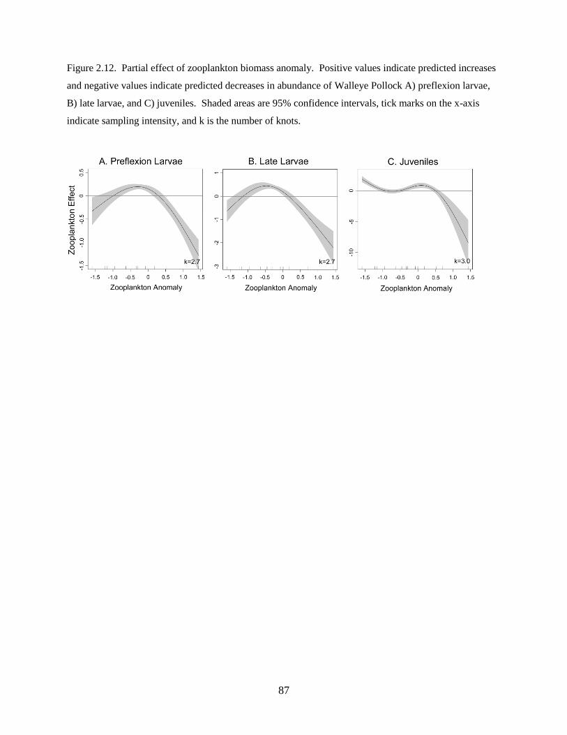
87
Figure 2.12. Partial effect of zooplankton biomass anomaly. Positive values indicate predicted increases
and negative values indicate predicted decreases in abundance of Walleye Pollock A) preflexion larvae,
B) late larvae, and C) juveniles. Shaded areas are 95% confidence intervals, tick marks on the x-axis
indicate sampling intensity, and k is the number of knots.
88
Chapter 3: Alternating Temperature States Influence Walleye Pollock (Gadus chalcogrammus)
Early Life Stages in the Southeastern Bering Sea
T. I. Smart1, 3,*
, J. T. Duffy-Anderson2, J. K. Horne
1
1School of Aquatic and Fishery Sciences, University of Washington, Seattle, Washington 98195, USA
2Recruitment Assessment and Conservation Engineering Division, Recruitment Processes Program,
Alaska Fisheries Science Center, National Marine Fisheries Service, National Oceanic and Atmospheric
Administration, Seattle, Washington 98115, USA
3Present address: Marine Resources Research Institute, South Carolina Department of Natural Resources,
Charleston, South Carolina 29422, USA
Citation: Smart, T.I., Duffy-Anderson, J.T., Horne, J.K. 2012. Alternating climate states influence
Walleye Pollock life stages in the southeastern Bering Sea. Mar. Ecol. Prog. Ser. 455: 257-267.
89
Abstract
Water temperatures in the southeastern Bering Sea influence the density of Walleye Pollock Gadus
chalcogrammus early life stages, potentially influencing spatial distributions and the phenology of
reproduction and development. We quantified stage-specific changes in spatial and temporal distributions
under cold- and warm-water conditions using generalized additive models. Analyses showed that Walleye
Pollock egg and yolksac larval spatial distributions are unaffected by temperature, suggesting that
spawning locations are stable. Preflexion larvae, late larvae, and juveniles shift onto the shelf under warm
conditions, similar to spatial shifts observed in distributions of sub-adults and adults. Temporal
distributions were used to address the hypothesis that timing of the density peak at each stage is delayed
under cold conditions. Differences in the timing of density peaks supported the hypothesis that the timing
of spawning, hatching, larval development, and juvenile transition are temperature-dependent. The
current analysis represents the best support available for the importance of temperature to Walleye
Pollock in determining early life stage development and population trends in the eastern Bering Sea. Our
data indicate that future changes in water temperatures could influence the early life stages of an
ecologically dominant member of the Bering Sea community by changing phenology and habitat use in
the first several months of life.
90
Introduction
In the eastern Bering Sea, interannual variation in the extent of sea ice over the continental shelf
determines water temperatures during the spring and summer when many fish species reproduce (Hunt &
Stabeno 2002). Gadus chalcogrammus (Walleye Pollock, hereafter pollock) is one of the most common
spring and summer shelf-spawning species in the Bering Sea ecosystem. Juvenile and adult populations
change in abundance and distribution in response to changes in water temperatures. Juvenile pollock (<
130 mm fork length) densities in surface trawls were higher and spatial distributions were broader during
two recent warm summers relative to two recent cold summers (Moss et al. 2009). The authors
hypothesized that warm conditions promote growth and survival in this population. Sub-adult (< 30 cm
fork length) and adult biomasses and spatial distributions have been shown to correlate with summer
temperature during the pollock post-spawning feeding season (Kotwicki et al. 2005). Biomass increased
with summer temperatures and the feeding migration progressed farther north and inshore (east) from
spawning grounds as temperature increased. Kotwicki et al. (2005) hypothesized that warmer water
temperatures advance the post-spawning feeding migration by advancing the timing of spawning. They
did not address the alternate hypothesis that spawning distribution changes in response to temperature
conditions.
Colder-than-average years are characterized by late sea-ice retreat from the shelf in the spring,
water column temperatures < 2 ºC over the shelf during spring and summer, and abundant large-bodied
zooplankton (Hunt et al. 2002, Coyle et al. 2011). Warmer-than-average years are characterized by early
ice retreat, continental shelf water temperatures > 2 ºC during spring and summer, and small-bodied
zooplankton. Sea-ice conditions also determine the extent and location of a pool of cold bottom water in
the summer over the middle shelf (50 – 100 m depth, Stabeno et al., 2012a). Pollock distributions
generally are restricted to areas > 2 ºC, such as those found outside the cold pool (Wyllie-Echeverria &
Wooster 1998). Therefore, in warm years, a larger area of thermally-suitable habitat is available to
pollock over the continental shelf, particularly over the middle shelf.
Smart et al. (2012) identified temperature in spring and summer as a leading environmental factor
influencing stage-specific densities of pollock early life stages (ELS) in the southeastern Bering Sea
(SEBS). Lower than average temperature years have high densities of eggs and newly hatched yolksac
larvae, regardless of the size of the adult spawning population. Average and higher-than-average
temperature years have high densities of feeding larvae (pre- and postflexion) and early juveniles (< 65
mm standard length). One hypothesis to explain the oscillation between early and developed stages is
high egg production under cold conditions. Spawning stock biomass in recent cold years has been low,
while egg densities have been high (Ianelli et al. 2009, Smart et al., 2012). An alternate hypothesis is that
the oscillation between early and late stages results from shifts in spawning and development phenology.
91
Maturity stage of SEBS pollock females in late winter tends to be advanced in warm relative to cold years
(Smart et al., 2012), although the impact of temperature on spawning has not been rigorously tested.
Temperature influences time to hatching in laboratory-reared Bering Sea pollock eggs with eggs at 2 ºC,
typical of cold conditions, requiring almost a week longer to hatch than eggs raised at 3.8 ºC, typical of
warm conditions (Blood 2002). In the Gulf of Alaska, lower than average temperatures contribute to high
mortality rates of field-observed larvae (Bailey et al. 1995).
The current study has two objectives: 1) to determine whether pollock ELS undergo spatial shifts
in response to changing temperature conditions and 2) to test whether temperature affects the phenology
of developmental events. Temperature can affect the annual distribution and development of pollock
ELS through the location of spawning, post-spawning transport, the timing of spawning, and rates of
development.
Materials and Methods
Field Surveys
The SEBS is bordered to the east by the Alaska mainland, to the south by the Alaska Peninsula
and eastern Aleutian Islands, to the west by the Aleutian Basin, and to the north by a change in vertical
structure of the water column and hydrography near 60º N latitude (Stabeno et al. 2012, b, Figure 3.1).
The shelf in the SEBS is very broad (~500 nautical miles). Northwest flow is driven by the Bering Slope
Current and flow through Aleutian passes (Napp et al. 2000). East-west flow is driven by the Aleutian
North Slope Current. The SEBS shelf can be divided into 3 bathymetric domains, each with its own
characteristic hydrography (Coachman 1986). The inner shelf (or coastal domain, < 50 m) is weakly
stratified and influenced by freshwater run-off; the middle shelf (50 – 100 m) is strongly stratified and
home to the cold pool in summer; and the outer shelf (100 – 200 m) is an area of intermittent upwelling in
the spring and summer, high productivity, and stratification (Hunt et al. 2002).
Depth-integrated densities (number 10 m-2
) of pollock ELS were determined from a time series of
ichthyoplankton surveys conducted by the NOAA Alaska Fisheries Science Center EcoFOCI program
(Seattle, WA, cf. Matarese et al. 2003). Surveys varied in spatial and temporal coverage and in the
number of tows conducted and gears used. To account for these variations, we limited the tows
considered for analysis to include pollock spawning areas, areas of potential transport, and the spawning
season. Data were limited to tows conducted south of 60 N latitude and east of the Aleutian basin, where
a majority of spawning occurs (Figure 3.1). Pollock spawning in the SEBS occurs from February through
November (Bacheler et al. 2010), but since sampling at the start or end of the spawning season is rare, we
92
limited catch records to between March and September (Figure 3.2). Fifteen years in the time series met
these spatial and temporal criteria (see Table 3.1 for details).
Gear types examined included obliquely towed bongo nets, a 1-m-2
multiple opening and closing
net and environmental sensing system (MOCNESS), and 1-m Tucker trawls, all equipped with 333 or 505
µm mesh. Differences in selectivity between bongo, MOCNESS, and Tucker gears are generally minor
and are appropriate for the length ranges of pollock examined in this study (Wiebe et al. 1976, Shima &
Bailey 1994). Volume filtered by each gear type was determined by calibrated flow meters mounted in
the mouth of each net. Catches were divided into 5 developmental stages: eggs, yolksac larvae (< 4.4 mm
standard length, SL), preflexion larvae (4.5 – 9.9 mm SL), late larvae (10.0 – 24.5 mm SL), and early
juveniles (25 – 64.5 mm SL). Divisions were based on standard length and developmental attributes
outlined in the Ichthyoplankton Information System (http://access.afsc.noaa.gov/ichthyo/index.cfm). The
upper size limit for early juveniles was selected based on the reduced catchability of larger fish with the
current gear types.
Monthly mean sea surface temperatures in May are a good indicator of overall conditions
throughout the pollock spawning period, correlating with both sea-ice state and summer temperatures
(Moss et al. 2009, Stabeno et al. 2012a). Sea surface temperature anomalies were derived from means of
monthly sea surface temperatures in May averaged over the area 54.3 – 60.0 ºN and 161.2 – 172.5 ºW
(NCEP/NCAR Reanalysis, Kalnay et al. 1996). The anomaly used in the current analysis is the deviation
from the mean value (2.11 ºC) for the survey years from 1988 – 2009, normalized by the standard
deviation (0.82 ºC).
Spatial Distributions
Stage-specific spatial distributions were determined for each ELS using variable-coefficient
generalize additive models (VCGAMs). VCGAMs allow the formulation of a nonparametric, nonlinear
regression model in which the effect of predictor variable can be determined for a specific location
(Hastie & Tibshirani 1993, Bacheler et al. 2009). In our case, we examined if density at each ELS was
expected to increase or decrease with an increase in annual sea surface temperature anomaly for a given
location. VCGAMs quantified changes in density for each ELS using the following model structure:
Ci = offset(volume) + a + s(SSB) + s(DOY) + s(location) + SSTa + s(location) · SSTa + ε (1)
where Ci is the count at stage i in each tow standardized (offset) by the volume of water filtered in each
tow (volume, m3), a is the model intercept, SSB is the annual female spawning stock biomass (tons)
included to account for annual changes in spawning effort, DOY is the day of year of each tow, location
is a combined term of the latitude and longitude for each tow, SSTa is the annual sea surface temperature
93
anomaly, and ε is the model error. SSB was based on summer surveys for adult pollock over the eastern
Bering Sea shelf (Ianelli et al. 2009). In preliminary examination of the data, there was no relationship
between temperature and SSB (T. Smart, unpubl.). The negative binomial error distribution was used
because of overdispersion caused by a high number of zeroes in the data set (Dupont 2002, Maunder and
Punt 2004). The negative binomial error distribution also produced the best model fit using the Akaike
Information Criterion (AIC) compared to Poisson, gamma, or Gaussian error distributions. The identity
link function was used in all VCGAMs. The level of smoothing was minimized to between 1 and 4 knots
to minimize the effects of spatial autocorrelation (Stige et al. 2006, Heinenän et al. 2008). All models
were coded and analyzed using the mgcv library (version 1.4-1, Wood 2006) in R (version 2.7.1, R
Development Core Team 2008). VCGAM predictions were plotted for each 0.1° by 0.1° degree cell for
which data were available in our study area.
Temporal Distributions
Generalized additive models (GAMs) were used to describe the non-linear temporal distributions
for each stage to estimate temporal shifts between temperature categories. Years of positive SSTa were
categorized as warm years (n = 6) and years of negative SSTa were categorized as cold years (n = 9).
This method was chosen over the Kolmogorov-Smirnoff test, as the Kolmogorov-Smirnoff test cannot
separate changes in peaks in the distribution from changes in the shapes of the distribution. GAMs allow
a visual comparison of the shapes and peaks in density among collection dates. The use of GAMs also
allowed us to account for the spatial component of our surveys, as tow locations often varied among
months and years. GAMs quantified anomalies in density for each ELS using:
Ci = offset(volume) + a + s(SSB) + factor(temperature) + s(location) + s(DOY) + ε (2)
where Ci is the count of stage i in each tow standardized (offset) by the volume of water filtered in each
tow (volume, m3), a is the model intercept, SSB is the annual female spawning stock biomass (tons),
temperature is the temperature category (cold or warm), location is a combined term of the latitude and
longitude for each tow, DOY is the day of year of each tow, and ε is the model error. The negative
binomial error distribution produced the best model fit based on AIC compared to the Poisson, gamma, or
Gaussian error distributions. The identity link function was used in all models. The level of smoothing
was minimized to between 1 and 4 knots to minimize the effects of spatial autocorrelation (Stige et al.
2006, Heinenän et al. 2008). When the effect of temperature category on density anomaly was significant
(α = 0.05), we derived the partial effect of DOY on the density anomaly within each temperature category
to define the temporal distribution. The switch from negative to positive density anomalies indicated the
DOY when each stage first appeared in surveys. The switch back to negative anomalies indicated the
DOY when each stage of development was complete (i.e. the season for each stage). The maximum
94
positive density anomaly predicted from DOY in GAMs indicated when each stage reached its maximum
density within each temperature category.
Results
Spatial Distributions
Egg densities were high across much of the study area in cold years, with highest catches near Unimak
Pass and the Pribilof Islands (Figure 3.3A). Tows with high egg density were common off the shelf in
1988 and 1990 and sporadic over the shelf in the rest of the warm years. High-density catches of yolksac
larvae were common over the shelf and around the Pribilof Islands in cold years and either over the basin
or over the shelf in warm years (Figure 3.3B). Preflexion larval densities were highest over the shelf and
near the Pribilof Islands in cold years and over the shelf and basin in warm years (Figure 3.3C). Highest
densities of late larvae were found near the Pribilof Islands in cold years and over the shelf in warm years
(Figure 3.3D). Very few tows collected juveniles in high numbers in cold years, but these tows occurred
mostly near the Pribilof Islands (Figure 3.3E). In warm years, high-density juvenile catches occurred
over the shelf and near the Pribilof Islands.
For all stages, annual temperature anomaly had a significant impact on location-specific density
(Table 3.2). Eggs and yolksac larvae were predicted to decrease in density as temperature increased in all
study area locations (Figure 3.4A, B). Preflexion larvae were predicted to increase in density as
temperature increased in the central portion of our study area (shelf break, outer shelf, middle shelf) and
decrease in density over the basin and in the inner shelf (Figure 3.4C). Late larval density decreased with
warming over the basin and to the north and increased over the shelf and to the south with warming
(Figure 3.4D). Warming did not impact juvenile density over the shelf, but was predicted to decrease
densities along the shelf break, over the basin, and to the north (Figure 3.4E).
Temporal Distributions
Temperature category affected the density of all pollock ELS in GAM analyses (Table 3.3). Egg density
anomalies peaked prior to DOY 150 (< June 1) in cold years and before DOY 140 (< May 20) in warm
years (Figure 3.5A). The yolksac larval season occurred between DOY 100 and 190 (Apr 10 – July 10) in
cold years and prior to DOY 175 (< June 25) in warm years (Figure 3.5B). Among preflexion larvae,
density anomalies peaked between DOY 100 and 195 (Apr 10 – July 15) in cold years and prior to DOY
185 (< July 5) in warm years (Figure 3.5C). The late larval season occurred between DOY 125 and 240
(May 5 – Aug 25) in cold years and between DOY 100 and 215 (Apr 10 – Aug 1) in warm years (Figure
3.5D). For juveniles, density anomalies peaked after DOY 130 (> May 10) in cold years and after DOY
120 (> May 1) in warm years (Figure 3.5E). For the stages that we can predict start or end dates of their
95
seasons, all seasons started or finished earlier in warm years than in cold years. However, as sampling
does not typically occur prior to March, we are unable to predict start dates for eggs, yolksac larvae in
warm years, and preflexion larvae in warm years. As sampling rarely occurs after October, we are unable
to predict end dates for juveniles. With these limitations, we cannot at present determine whether or not
the span of each stage is shortened in warm years as hypothesized.
Temporal shifts were estimated for each stage using the density maximum predicted by DOY.
Differences in maxima indicated delays in peak temporal distributions of all ELS in cold compared to
warm years (Table 3.4). These differences suggested a 40-d delay in the egg stage maxima (spawning
and hatching), a 45-d delay in the yolksac larval stage maxima (hatching and absorption of yolk reserves),
a 20-d delay in the preflexion stage maxima (feeding commences), a 30-d delay in the late larval stage
maxima (flexion of the notochord), and a 25-d delay in the juvenile stage maxima (completion of the
juvenile transition and growth to sizes above which our collection gear are avoided).
Discussion
Water temperatures in the southeastern Bering Sea influenced Walleye Pollock (Gadus
chalcogrammus) ELS in several ways. Spatial distributions of eggs and yolksac larvae were not affected
by temperature, while feeding stages (preflexion larvae, late larvae, and juveniles) were affected.
Variable-coefficient GAMs predicted decreases in the density of eggs and yolksac larvae with warming,
suggesting that there is no discernible shift in spawning locations. Variable-coefficient GAMs predicted
that densities of preflexion larvae and late larvae would increase over the shelf, while densities of
preflexion larvae, late larvae, and juveniles would decrease offshore, suggesting a movement of the
population onto the shelf. A likely mechanism to explain these patterns is that spawning location remains
relatively constant, but larval transport varies with temperature. Temporal distributions predicted by
GAMs indicated a delay in the timing of reproductive and ontogenetic events in cold temperatures.
Earlier spawning, hatching, and onset of feeding could explain the low densities of eggs and yolksac
larvae observed in warm years. We were unable to determine rates of development because of
uncertainty at the beginning and end of the sampling season. Our analysis suggests that in warm years
this population reaches the juvenile stage earlier and would have more time for feeding and growth prior
to the oncoming winter.
Spatial Distribution Shifts
Bacheler et al. (2012) found indications of shifts in pollock spawning location across the shelf
using an earlier time series and variable-coefficient GAMs. In support of this pattern, Anchovy
(Engraulis encrasicolus), Sardine (Sardina pilchardus), and Common Sole (Solea solea) have all been
reported to shift spawning locations in response to environmental factors (Bellier et al. 2007, Eastwood et
96
al. 2001). We were unable to discern the same pattern for pollock eggs. An alternate explanation is that
SEBS pollock spawning location does not, but subsequent transport of ELS does. The current study
supplements the findings of Bacheler et al. (2012) with spatial shifts in subsequent ELS, which can isolate
differential transport from shifts in spawning location. In cold years, surface currents are generally
westward and faster relative to warm years (Stabeno et al., 2012 a), which would transport larvae to the
outer shelf or offshore if they were spawned over the shelf. In warm years, larvae are more likely to be
retained over the shelf. Although we found only a small increase in juvenile density over the inner shelf
with warming, we did observe a large decrease in density offshore. Together, these results suggest that
juveniles move onshore in warm years although densities may be low and distributions are widespread.
We attribute distributions of larvae and early juveniles to shifts in subsequent transport rather than shifts
in spawning location (see also Duffy-Anderson et al. 2006).
Spatial shifts observed in pollock larvae and juveniles determine their use of two SEBS shelf
domains which vary in productivity and zooplankton communities. The shelf tends to have a greater
concentration of smaller copepods (more appropriate prey items for small larvae), while larger copepods
(appropriate prey items for large larvae) are generally found in spring over the deeper outer shelf (Cooney
& Coyle 1982, Vidal & Smith 1986, Baier & Napp 2003). Zooplankton present in the SEBS during cold
years are larger, energetically richer, and are concentrated over the outer shelf and shelf break (Coyle et
al. 2011). Cold temperatures favor a larger-bodied prey for late larvae and juveniles and are predicted to
increase juvenile survival if they can exploit this resource. Warm water temperatures with a smaller-sized
prey field are predicted to benefit the growth of preflexion larvae, which are gape-limited (Nakatani
1988). In warm years, preflexion larvae are more likely to be in the vicinity of small prey over the shelf.
In cold years, late larvae and juveniles are more likely to be in the vicinity of large prey over the shelf
break. This hypothesis is supported by recent evidence that the few juvenile pollock collected in recent
cold years in the SEBS were energetically richer than those sampled in recent warm years (Hunt et al.,
2011). The spatial distribution shifts observed in the current study combined with the observation of
spatially-distinct zooplankton communities supports the hypothesis that prey fields in cold years should
support higher densities and energetically richer pollock larvae and juveniles.
Phenological Shifts
Pollock ELS oscillate between high densities of early stages (eggs and yolksac larvae) in cold
years and high densities of developed stages (preflexion and late larvae and juveniles) in warm years
(Smart et al. 2012). One explanation for high numbers of early-staged individuals in cold years is a
combination of delayed spawning and slower rates of development. Egg density temporal distribution is
dependent on both the timing of spawning and the time required to develop to the hatching stage. Based
on observed egg temporal distributions, either the timing of spawning events or development to hatching
97
is temperature-dependent in the SEBS. There are currently no data available on the temperature-
dependence of gametogenesis in pollock. As a comparison, maturation rates and spawning in Atlantic
Cod (Gadus morhua) are temperature-dependent, and completion of maturation is advanced by several
weeks in warm temperatures (Beaugrand et al. 2003, Yoneda & Wright 2005). Extrapolating from
laboratory data, Blood (2002) estimated that egg incubation period could be delayed by 13 d during a cold
(1997) compared to a warm (1998) year. In the field, the estimated delay in peak egg density is 40 d,
suggesting that both timing of spawning and development could be delayed, accounting for the interval
between temperature categories in the current study.
Comparing temperature categories, we found evidence of temperature-dependence in the timing
of hatching, onset of feeding, flexion of the notochord, juvenile transition, or some combination of
temperature-dependence among any of these developmental events. Delayed hatching increases the
likelihood of collecting eggs during our primary sampling period (May through September). Delayed
onset of feeding retains larvae in the non-feeding yolksac stage. Jung et al. (2006) estimated that hatching
was delayed by 12 – 17 d in 1976 (cold) compared to 1977 (warm) based on the staging of field-caught
eggs. Under warm conditions, early-spawned eggs should rapidly develop and hatch. The newly hatched
larvae could consume their yolk reserves in perhaps as little as a week (Walline 1985, Porter & Theilacker
1999). Temperature-dependent development rates in larval stages have consequences for matching with
prey production cycles and for growth-dependent mortality (Gallego & Heath 1997). Currently, we
cannot estimate start and end points and by extension the time span of development, for all stages.
Therefore, the timing of events must stand as a proxy supporting the hypothesis that development is
delayed in cold temperatures relative to warm water temperatures.
In summary, our data demonstrated that Walleye Pollock ELS in the southeastern Bering Sea
responded to changes in oceanographic conditions (i.e. water temperature and flows) by shifting density
distributions in time and, in some cases, space. The temperature-associated oscillation between high egg
and yolksac larval density and high density of more developed larvae and juveniles can be explained by
phenological shifts in spawning and development. Distributions of pollock feeding larvae and juveniles
also spatially shifted between two habitats, the continental shelf and the shelf break or offshore, which has
the potential to affect access to appropriate sized prey. We hypothesize that the lack of spatial shifts
observed in pollock eggs and early larvae indicate that adults do not adjust the location of spawning in
response to temperature. We further hypothesize that spatial shifts observed in larval and juvenile
densities reflect differences in transport between cold and warm years. Comparable trends among life
stages suggest shared habitats. As temperatures continue to change in the North Pacific, identification of
spatiotemporal shifts in habitat use will be crucial to understanding short- and long-term population
trends in this ecologically and economically important species.
98
Acknowledgements
Thanks to the members of NOAA’s Ecosystems and Fisheries Oceanography Coordinated Investigations
(EcoFOCI) who were involved in the collection and processing of the ichthyoplankton samples. L.
Ciannelli (Oregon State University) assisted with statistical analyses and interpretation. This research
was supported by the Bering Sea Integrated Ecosystem Research program (BSIERP) of the North Pacific
Research Board and the North Pacific Climate Regimes and Ecosystem Productivity (NPCREP) program
of the National Oceanographic and Atmospheric Administration. This paper is EcoFOCI Contribution
No. N754 – RAOA – 0, BEST-BSIERP Publication No. 35. We appreciate comments by Jeffrey Napp,
Ann Matarese, and three anonymous reviewers. The findings and conclusions in the paper are those of
the authors and do not necessarily represent the views of the National Marine Fisheries Service.
99
Literature Cited
Bacheler NM, Ciannelli L, Bailey KM, Duffy-Anderson JT (2010) Spatial and temporal patterns of
Walleye Pollock spawning in the eastern Bering Sea inferred from egg and larval distributions.
Fish Oceanogr 19:107-120
Bacheler NM, Ciannelli L, Bailey K, Bartolino V (2012) Do Walleye Pollock exhibit flexibility in where
or when they spawn based on variability in water temperature? Deep-Sea Res II 65-70: 208-216
Baier CT, Napp JM (2003) Climate-induced variability in Calanus marshallae populations. J Plank Res
25:771-782
Bailey KM, Canino MF, Napp JM, Spring SM, Brown AL (1995) Contrasting years of prey levels,
feeding conditions and mortality of larval Walleye Pollock Theragra chalcogramma in the
western Gulf of Alaska. Mar Ecol Prog Ser 119:11-23
Beaugrand G, Brander KM, Souissi JALS, Reid PC (2003) Plankton effect on cod recruitment in the
North Sea. Nature 426:661-664
Bellier E, Planque B, Petitgas P (2007) Historical fluctuations in spawning location of Anchovy
(Engraulis encrasicolus) and Sardine (Sardina pilchardus) in the Bay of Biscay during 1967-73
and 2000-2004. Fish Oceanogr 16:1-15
Blood DM (2002) Low-temperature incubation of Walleye Pollock (Theragra chalcogramma) eggs from
the southeastern Bering Sea shelf and Shelikof Strait, Gulf of Alaska. Deep-Sea Res II 49:6095-
6108
Coachman LK (1986) Circulation, water masses, and fluxes on the southeastern Bering Sea shelf.
Continental Shelf Res 5(1-2):23-108
Cooney RT, Coyle KO (1982) Trophic implications of cross-shelf copepod distributions in the
southeastern Bering Sea. Mar. Biol. 70:187-196
Coyle KO, Eisner LB, Mueter FJ, Pinchuk AI, Janout MA, Cieciel KD, Farley EV, Andrews AG (2011)
Climate change in the southeastern Bering Sea: impacts on pollock stocks and implications for
the oscillating control hypothesis. Fish Oceanogr 20:139-156
Duffy-Anderson JT, Busby MS, Mier KL, Deliyanides CM, Stabeno PJ (2006) Spatial and temporal
patterns in summer ichthyoplankton assemblages on the eastern Bering Sea shelf 1996-2000.
Fish Oceanogr 15:80-94
Dupont WD (2002) Statistical Modelling for Biomedical Researchers: A Simple Introduction to the
Analysis of Complex Data. Cambridge Press, New York, 522 pp.
100
Eastwood PD, Meaden GJ, Grioche A (2001) Modeling spatial variations in spawning habitat suitability
for the sole Solea solea using regression quantiles and GIS procedures. Mar Ecol Prog Ser
224:251-266
Gallego A, Heath M (1997) The effect of growth-dependent mortality, external environment and internal
dynamics of larval fish growth: An individual-based modeling approach. J Fish Biol 51:121-134
Hastie T, Tibshirani R (1993) Varying-coefficient models. J R Stat Soc B 55:757-796
Heinenän S, Rönkä M, von Numers M (2008) Modelling the occurrence and abundance of a colonial
species, the arctic tern Sterna paradisaea in the archipelago of SW Finland. Ecography 31:601-
611
Hunt GL, Stabeno PJ (2002) Climate change and the control of energy flow in the southeastern Bering
Sea. Prog Oceanogr 55:5-22
Hunt GL, Stabeno PJ, Walters G, Sinclair E, Brodeur RD, Napp JM, Bond NA (2002) Climate change
and control of the southeastern Bering Sea pelagic ecosystem. Deep-Sea Res II 49:5821-5853
Hunt GL, Coyle KO, Eisner LB, Farley E, Heintz R, Mueter F, Napp JM, Overland JE, Ressler PH, Salo
S, Stabeno PJ (2001). Climate impacts on eastern Bering Sea food webs: A synthesis of new data
and an assessment of the Oscillating Control Hypothesis. ICES J Mar Sci 68: 1230-1243
Ianelli JN, Barbeaux S, Honkalehto T, Kotwicki S, Aydin K, Williamson N (2009). Assessment of the
Walleye Pollock stock in the Eastern Bering Sea. In: Stock assessment and fishery evaluation
report for the groundfish resources of the Bering Sea/Aleutian Islands regions. North Pac. Fish.
Mgmt. Council, Anchorage, AK, section 1, 49-148
Ichthyoplankton Information System. National Oceanic and Atmospheric Administration. Accessed 23
July. http://access.afsc.noaa.gov/ichthyo/index.cfm
Jung KM, Kang S, Kim S, Kendall AW (2006) Ecological characteristics of Walleye Pollock eggs and
larvae in the southeastern Bering Sea during the late 1970s. J Oceanogr 62:859-871
Kalnay E, Kanamitsu M, Kistler R, Collins W, Deaven D, Gandin L, Iredell M, Saha S, White G,
Woollen J, Zhu Y, Leetmaa A, Reynolds B, Chelliah M, Ebisuzaki W, Higgins W, Janowiak J,
Mo K, Ropelewski C, Wang J, Jenne R, Joseph D (1996) The NCEP/NCAR 40-year reanalysis
project. Bull Am Meteorolog Soc 77:437–471
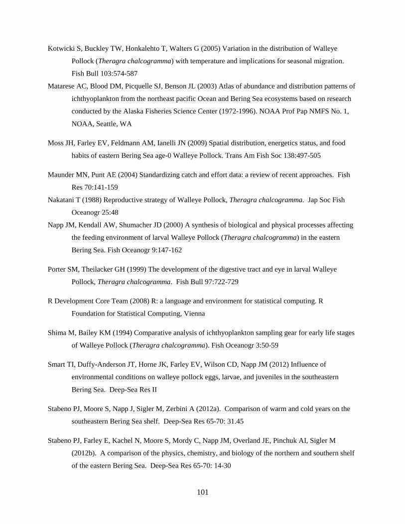
101
Kotwicki S, Buckley TW, Honkalehto T, Walters G (2005) Variation in the distribution of Walleye
Pollock (Theragra chalcogramma) with temperature and implications for seasonal migration.
Fish Bull 103:574-587
Matarese AC, Blood DM, Picquelle SJ, Benson JL (2003) Atlas of abundance and distribution patterns of
ichthyoplankton from the northeast pacific Ocean and Bering Sea ecosystems based on research
conducted by the Alaska Fisheries Science Center (1972-1996). NOAA Prof Pap NMFS No. 1,
NOAA, Seattle, WA
Moss JH, Farley EV, Feldmann AM, Ianelli JN (2009) Spatial distribution, energetics status, and food
habits of eastern Bering Sea age-0 Walleye Pollock. Trans Am Fish Soc 138:497-505
Maunder MN, Punt AE (2004) Standardizing catch and effort data: a review of recent approaches. Fish
Res 70:141-159
Nakatani T (1988) Reproductive strategy of Walleye Pollock, Theragra chalcogramma. Jap Soc Fish
Oceanogr 25:48
Napp JM, Kendall AW, Shumacher JD (2000) A synthesis of biological and physical processes affecting
the feeding environment of larval Walleye Pollock (Theragra chalcogramma) in the eastern
Bering Sea. Fish Oceanogr 9:147-162
Porter SM, Theilacker GH (1999) The development of the digestive tract and eye in larval Walleye
Pollock, Theragra chalcogramma. Fish Bull 97:722-729
R Development Core Team (2008) R: a language and environment for statistical computing. R
Foundation for Statistical Computing, Vienna
Shima M, Bailey KM (1994) Comparative analysis of ichthyoplankton sampling gear for early life stages
of Walleye Pollock (Theragra chalcogramma). Fish Oceanogr 3:50-59
Smart TI, Duffy-Anderson JT, Horne JK, Farley EV, Wilson CD, Napp JM (2012) Influence of
environmental conditions on walleye pollock eggs, larvae, and juveniles in the southeastern
Bering Sea. Deep-Sea Res II
Stabeno PJ, Moore S, Napp J, Sigler M, Zerbini A (2012a). Comparison of warm and cold years on the
southeastern Bering Sea shelf. Deep-Sea Res 65-70: 31.45
Stabeno PJ, Farley E, Kachel N, Moore S, Mordy C, Napp JM, Overland JE, Pinchuk AI, Sigler M
(2012b). A comparison of the physics, chemistry, and biology of the northern and southern shelf
of the eastern Bering Sea. Deep-Sea Res 65-70: 14-30
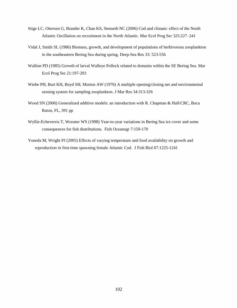
102
Stige LC, Ottersen G, Brander K, Chan KS, Stenseth NC (2006) Cod and climate: effect of the North
Atlantic Oscillation on recruitment in the North Atlantic. Mar Ecol Prog Ser 325:227–241
Vidal J, Smith SL (1986) Biomass, growth, and development of populations of herbivorous zooplankton
in the southeastern Bering Sea during spring. Deep-Sea Res 33: 523-556
Walline PD (1985) Growth of larval Walleye Pollock related to domains within the SE Bering Sea. Mar
Ecol Prog Ser 21:197-203
Wiebe PH, Burt KH, Boyd SH, Morton AW (1976) A multiple opening/closing net and environmental
sensing system for sampling zooplankton. J Mar Res 34:313-326
Wood SN (2006) Generalized additive models: an introduction with R. Chapman & Hall/CRC, Boca
Raton, FL, 391 pp
Wyllie-Echeverria T, Wooster WS (1998) Year-to-year variations in Bering Sea ice cover and some
consequences for fish distributions. Fish Oceanogr 7:159-170
Yoneda M, Wright PJ (2005) Effects of varying temperature and food availability on growth and
reproduction in first-time spawning female Atlantic Cod. J Fish Biol 67:1225-1241
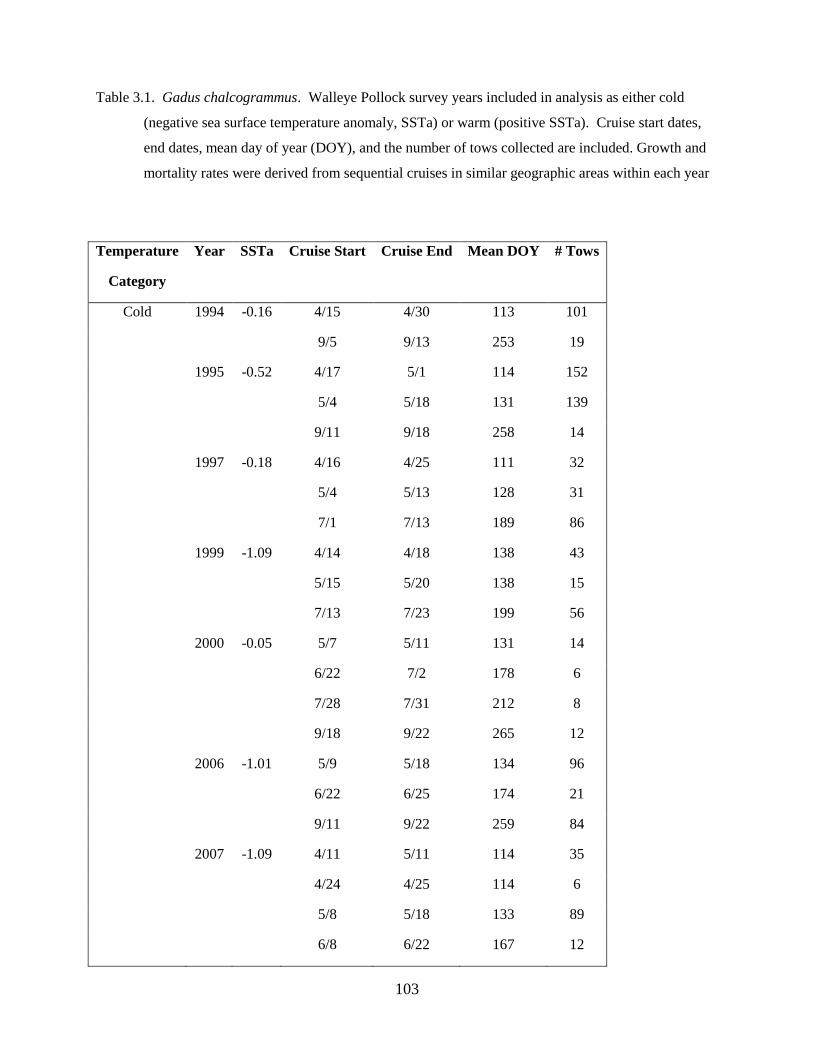
103
Table 3.1. Gadus chalcogrammus. Walleye Pollock survey years included in analysis as either cold
(negative sea surface temperature anomaly, SSTa) or warm (positive SSTa). Cruise start dates,
end dates, mean day of year (DOY), and the number of tows collected are included. Growth and
mortality rates were derived from sequential cruises in similar geographic areas within each year
Temperature
Category
Year SSTa Cruise Start Cruise End Mean DOY # Tows
Cold 1994 -0.16 4/15 4/30 113 101
9/5 9/13 253 19
1995 -0.52 4/17 5/1 114 152
5/4 5/18 131 139
9/11 9/18 258 14
1997 -0.18 4/16 4/25 111 32
5/4 5/13 128 31
7/1 7/13 189 86
1999 -1.09 4/14 4/18 138 43
5/15 5/20 138 15
7/13 7/23 199 56
2000 -0.05 5/7 5/11 131 14
6/22 7/2 178 6
7/28 7/31 212 8
9/18 9/22 265 12
2006 -1.01 5/9 5/18 134 96
6/22 6/25 174 21
9/11 9/22 259 84
2007 -1.09 4/11 5/11 114 35
4/24 4/25 114 6
5/8 5/18 133 89
6/8 6/22 167 12
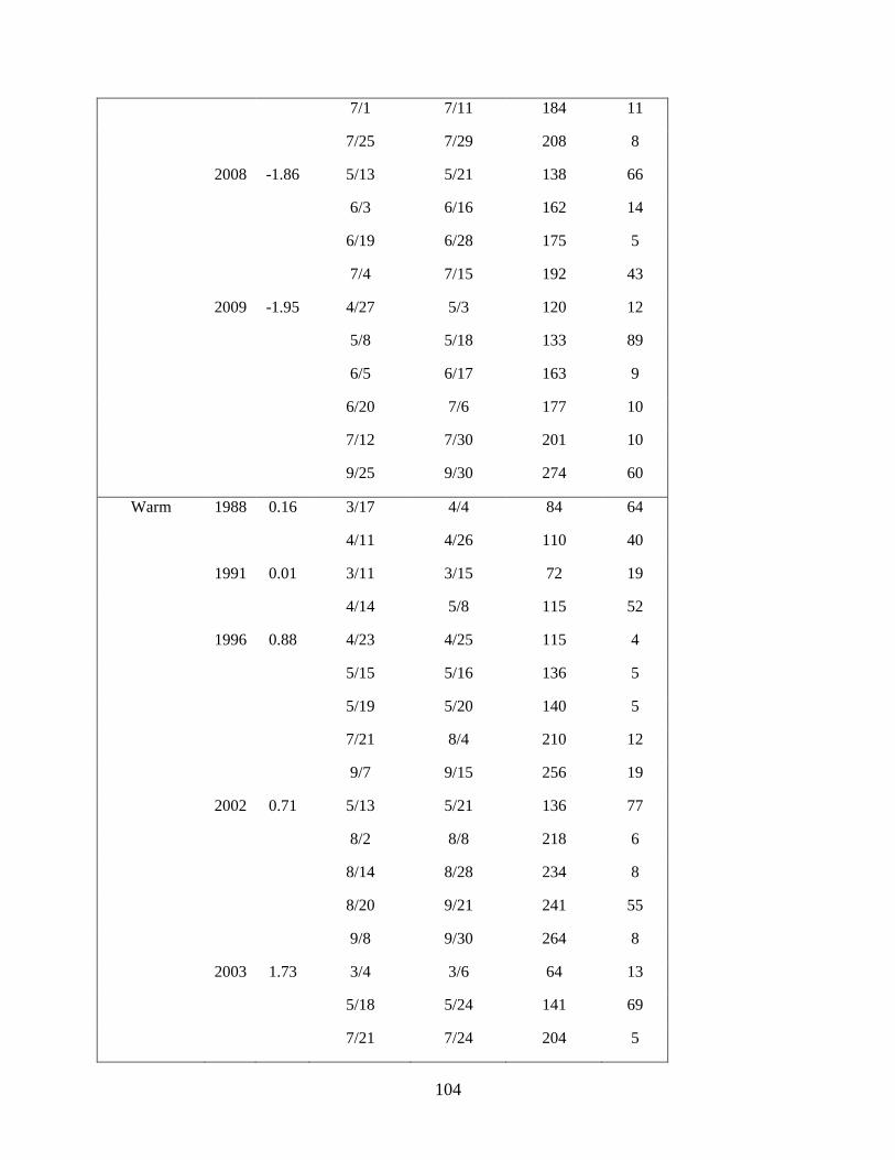
104
7/1 7/11 184 11
7/25 7/29 208 8
2008 -1.86 5/13 5/21 138 66
6/3 6/16 162 14
6/19 6/28 175 5
7/4 7/15 192 43
2009 -1.95 4/27 5/3 120 12
5/8 5/18 133 89
6/5 6/17 163 9
6/20 7/6 177 10
7/12 7/30 201 10
9/25 9/30 274 60
Warm 1988 0.16 3/17 4/4 84 64
4/11 4/26 110 40
1991 0.01 3/11 3/15 72 19
4/14 5/8 115 52
1996 0.88 4/23 4/25 115 4
5/15 5/16 136 5
5/19 5/20 140 5
7/21 8/4 210 12
9/7 9/15 256 19
2002 0.71 5/13 5/21 136 77
8/2 8/8 218 6
8/14 8/28 234 8
8/20 9/21 241 55
9/8 9/30 264 8
2003 1.73 3/4 3/6 64 13
5/18 5/24 141 69
7/21 7/24 204 5
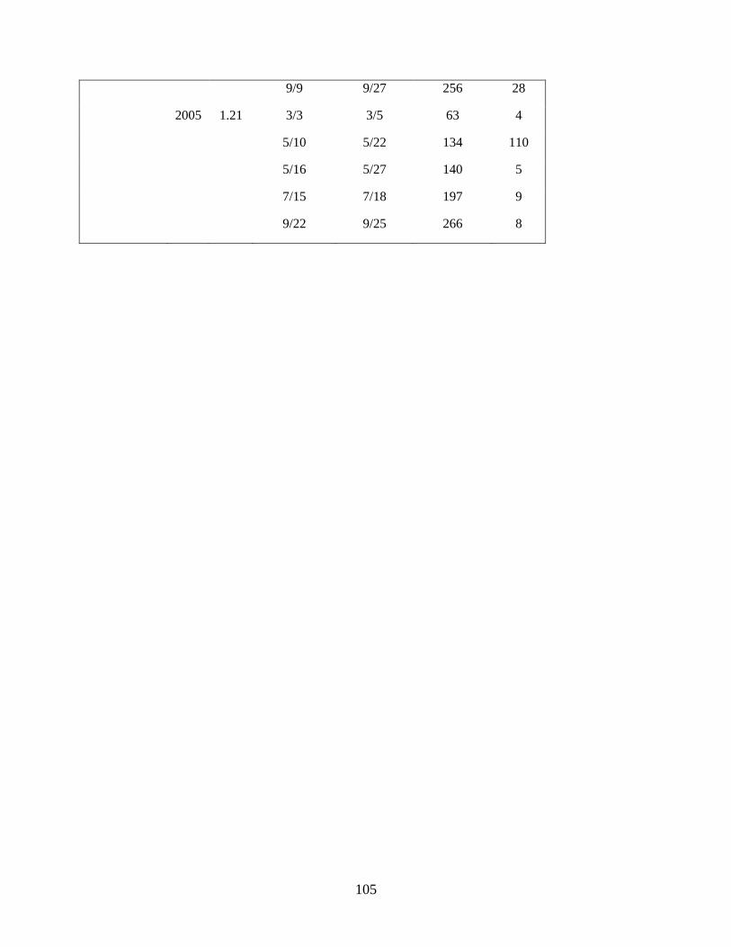
105
9/9 9/27 256 28
2005 1.21 3/3 3/5 63 4
5/10 5/22 134 110
5/16 5/27 140 5
7/15 7/18 197 9
9/22 9/25 266 8
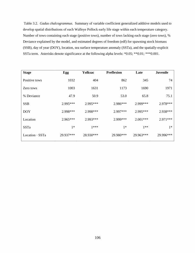
106
Table 3.2. Gadus chalcogrammus. Summary of variable coefficient generalized additive models used to
develop spatial distributions of each Walleye Pollock early life stage within each temperature category.
Number of tows containing each stage (positive tows), number of tows lacking each stage (zero tows), %
Deviance explained by the model, and estimated degrees of freedom (edf) for spawning stock biomass
(SSB), day of year (DOY), location, sea surface temperature anomaly (SSTa), and the spatially-explicit
SSTa term. Asterisks denote significance at the following alpha levels: *0.05; **0.01; ***0.001.
Stage Egg Yolksac Preflexion Late Juvenile
Positive tows 1032 404 862 345 74
Zero tows 1003 1631 1173 1690 1971
% Deviance 47.9 50.9 53.0 65.8 75.1
SSB 2.995*** 2.995*** 2.986*** 2.999*** 2.978***
DOY 2.998*** 2.998*** 2.997*** 2.995*** 2.938***
Location 2.965*** 2.993*** 2.999*** 2.001*** 2.971***
SSTa 1* 1*** 1* 1** 1*
Location · SSTa 29.937*** 28.930*** 29.980*** 29.963*** 29.996***
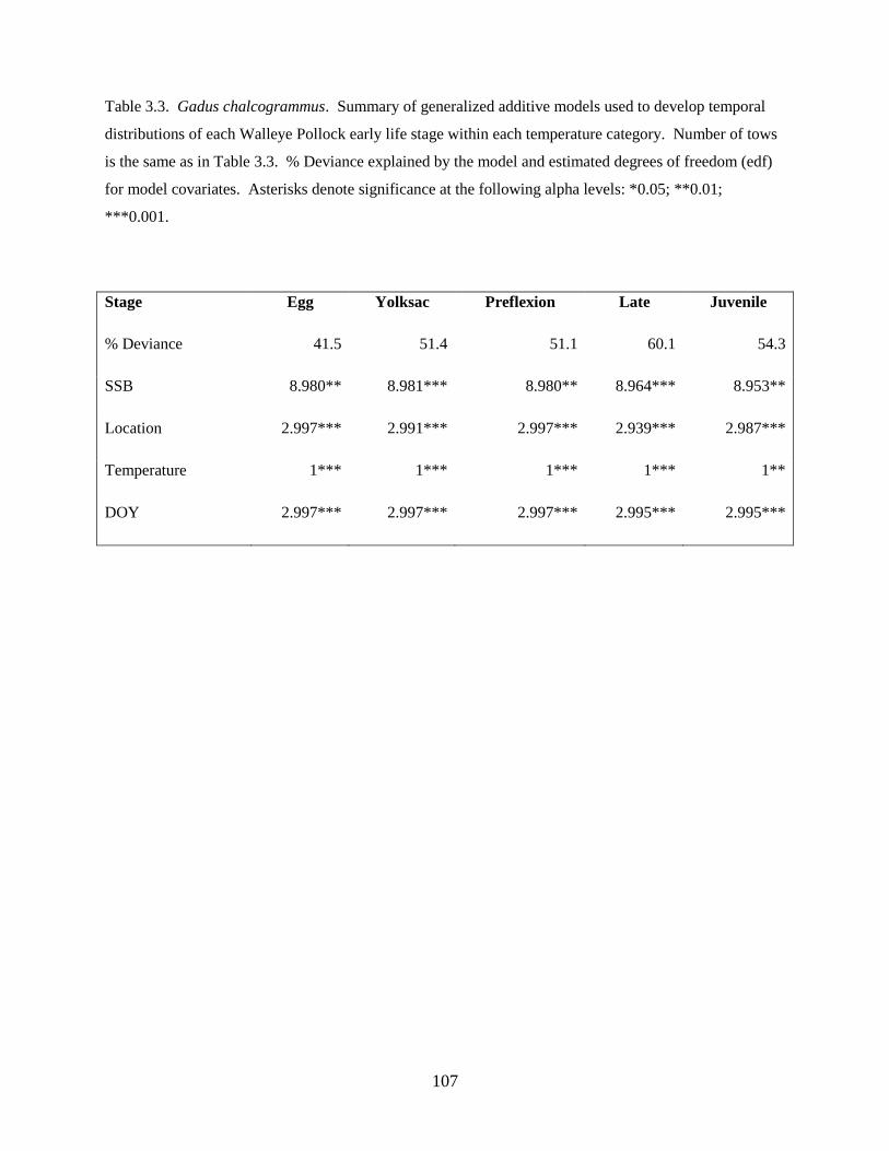
107
Table 3.3. Gadus chalcogrammus. Summary of generalized additive models used to develop temporal
distributions of each Walleye Pollock early life stage within each temperature category. Number of tows
is the same as in Table 3.3. % Deviance explained by the model and estimated degrees of freedom (edf)
for model covariates. Asterisks denote significance at the following alpha levels: *0.05; **0.01;
***0.001.
Stage Egg Yolksac Preflexion Late Juvenile
% Deviance 41.5 51.4 51.1 60.1 54.3
SSB 8.980** 8.981*** 8.980** 8.964*** 8.953**
Location 2.997*** 2.991*** 2.997*** 2.939*** 2.987***
Temperature 1*** 1*** 1*** 1*** 1**
DOY 2.997*** 2.997*** 2.997*** 2.995*** 2.995***
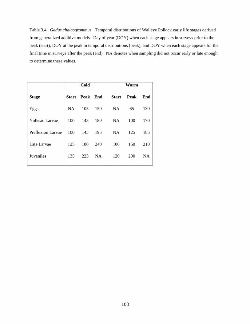
108
Table 3.4. Gadus chalcogrammus. Temporal distributions of Walleye Pollock early life stages derived
from generalized additive models. Day of year (DOY) when each stage appears in surveys prior to the
peak (start), DOY at the peak in temporal distributions (peak), and DOY when each stage appears for the
final time in surveys after the peak (end). NA denotes when sampling did not occur early or late enough
to determine these values.
Cold Warm
Stage Start Peak End Start Peak End
Eggs NA 105 150 NA 65 130
Yolksac Larvae 100 145 180 NA 100 170
Preflexion Larvae 100 145 195 NA 125 185
Late Larvae 125 180 240 100 150 210
Juveniles 135 225 NA 120 200 NA
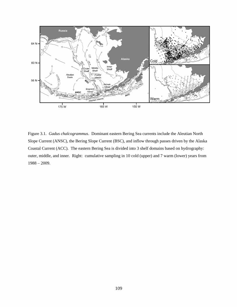
109
Figure 3.1. Gadus chalcogrammus. Dominant eastern Bering Sea currents include the Aleutian North
Slope Current (ANSC), the Bering Slope Current (BSC), and inflow through passes driven by the Alaska
Coastal Current (ACC). The eastern Bering Sea is divided into 3 shelf domains based on hydrography:
outer, middle, and inner. Right: cumulative sampling in 10 cold (upper) and 7 warm (lower) years from
1988 – 2009.
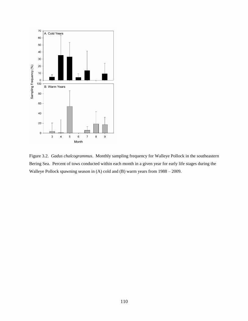
110
Figure 3.2. Gadus chalcogrammus. Monthly sampling frequency for Walleye Pollock in the southeastern
Bering Sea. Percent of tows conducted within each month in a given year for early life stages during the
Walleye Pollock spawning season in (A) cold and (B) warm years from 1988 – 2009.
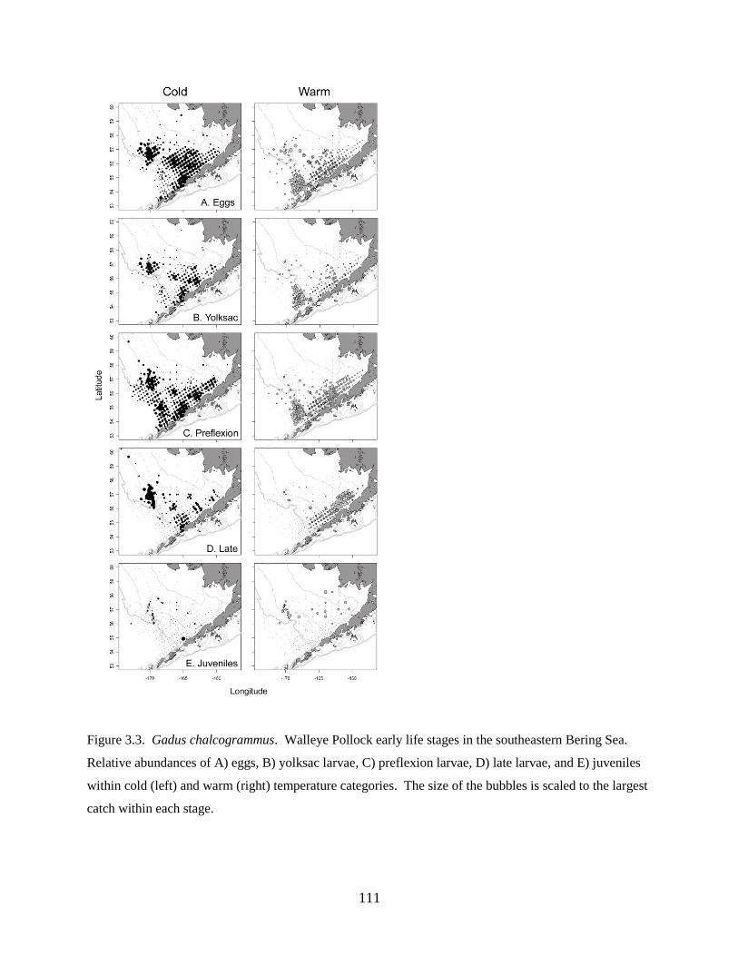
111
Figure 3.3. Gadus chalcogrammus. Walleye Pollock early life stages in the southeastern Bering Sea.
Relative abundances of A) eggs, B) yolksac larvae, C) preflexion larvae, D) late larvae, and E) juveniles
within cold (left) and warm (right) temperature categories. The size of the bubbles is scaled to the largest
catch within each stage.
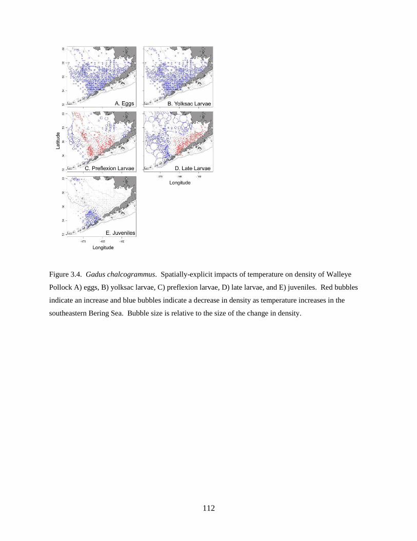
112
Figure 3.4. Gadus chalcogrammus. Spatially-explicit impacts of temperature on density of Walleye
Pollock A) eggs, B) yolksac larvae, C) preflexion larvae, D) late larvae, and E) juveniles. Red bubbles
indicate an increase and blue bubbles indicate a decrease in density as temperature increases in the
southeastern Bering Sea. Bubble size is relative to the size of the change in density.
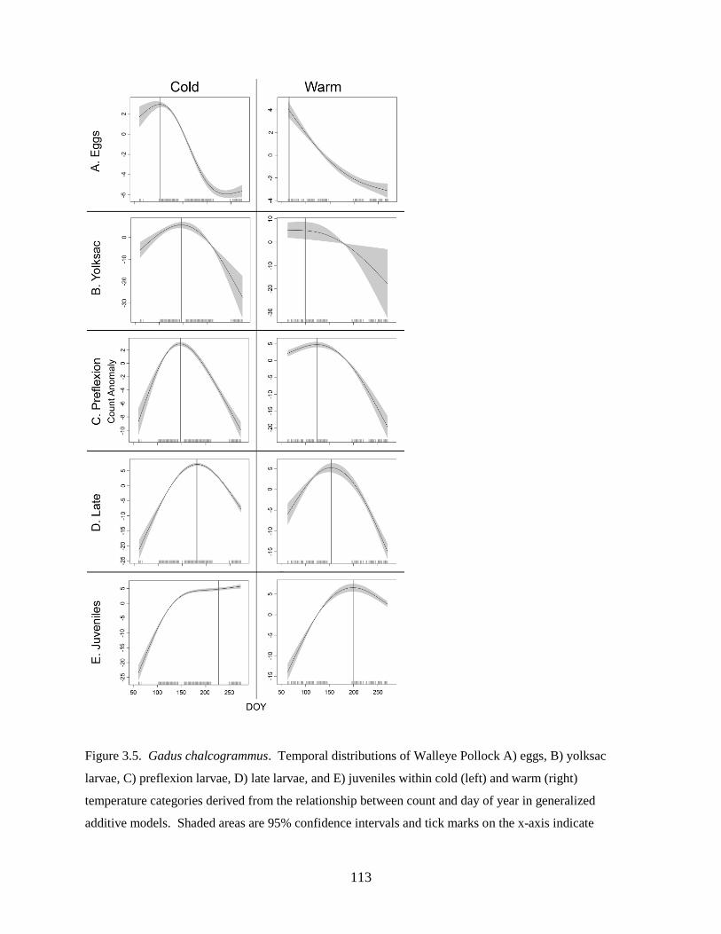
113
Figure 3.5. Gadus chalcogrammus. Temporal distributions of Walleye Pollock A) eggs, B) yolksac
larvae, C) preflexion larvae, D) late larvae, and E) juveniles within cold (left) and warm (right)
temperature categories derived from the relationship between count and day of year in generalized
additive models. Shaded areas are 95% confidence intervals and tick marks on the x-axis indicate

114
sampling intensity on each day of year (DOY). The vertical line denotes the estimated DOY of the
density maxima.
115
Chapter 4. Vertical distributions of the early life stages of Walleye Pollock (Gadus chalcogrammus)
in the southeastern Bering Sea
Smart, T.I.1,4
, Siddon, E.C.2, Duffy-Anderson, J.T.
3
1School of Aquatic and Fishery Sciences, University of Washington, Seattle, WA, 98195 USA
2Fisheries Division, School of Fisheries and Ocean Sciences, University of Alaska Fairbanks, Juneau,
AK, 99801 USA
3RACE Division, Recruitment Processes Program, Alaska Fisheries Science Center, NOAA Fisheries,
Seattle, WA, 98115 USA
4Current address: Marine Resources Research Institute, Charleston, South Carolina 29422 USA
Citation: Smart, T., Duffy-Anderson, J.T., and Siddon, E. 2013. Vertical distribution of early life stages
of walleye pollcok and implications for transport and connectivity. Deep-Sea Research II: Topical
Studies in Oceanography. 94: 201-201.
116
Abstract
The present study examines vertical distributions of the early life stages of Walleye Pollock (Gadus
chalcogrammus) in the Southeastern Bering Sea to assess ontogenetic and dielvertical migration in
relation to development and habitat. Walleye Pollock demonstrated a decrease in the depth of occurrence
following hatching, indicating an ontogenetic change in vertical distribution. Eggs occurred deepest in
the water column and early juveniles occurred shallowest. Vertical distributions were related to the date
of collection, water column depth, and thermocline depth. Non-feedingstages (eggs and yolksac larvae,
<4.5 mm standard length [SL]) did not exhibit diel vertical migration. Feeding larvae exhibited diel
vertical migration, although patterns varied between two feeding stages. Preflexion stage larvae (4.5–9.9
mm SL) were concentrated between 10 and 20 m during the day and deeper at night. Postflexion stage
larvae (flexion and postflexion, 10.0–24.5 mm SL) underwent regular diel migrations (0–20 m, night; 10–
40 m, day). Low sample sizes limited our ability to assess diel vertical migration in early juveniles, but
this stage tends to occur in the upper 20 m of the water column, regardless of time of day. These results
suggest that vertical distributions and diel migration potentially are driven by prey availability at
sufficient light levels for preflexion larvae to feed and a trade-off between prey access and predation risk
for postflexion larvae. Vertical distributions of eggs and preflexion larvae varied with habitat examined
(on the continental shelf versus over the continental slope). Vertical distributions of Walleye Pollock
eggs, yolksac larvae, and preflexion larvae in the Bering Sea are different from distributions in other
ecosystems, which can impact transport and modeling efforts.
117
Introduction
Information on vertical distributions of early life history stages of fishes is critical for accurate
modeling of larval transport to nursery habitats as transport can differ depending on vertical position in
the water column (Tanaka 1991, Stenevik et al. 2003, Fiksen et al. 2007, Miller 2007, Kristiansen et al.
2009). Ontogenetic vertical migration (OVM) is a pattern in which vertical distribution changes with
stage of development. Typically, OVM involves a shoaling in the depth of occurrence as eggs and larvae
develop, which allows larvae to exploit high food concentrations and fast currents in surface waters
(Fortier and Leggett 1983, Norcross and Shaw 1984, Hare and Govoni 2005). Often OVM is
accompanied by increasing complexity of vertical behaviors, such as responsiveness to changes in light
intensity (Heath et al. 1988, Hare and Govoni 2005). Diel vertical migration (DVM) is a behavioral trend
in which depth of occurrence changes with time of day and light intensity. DVM typically is exhibited by
feeding stages. Larval fish are visual predators, consuming a variety of zooplankton, and as such will
orient themselves in the water column to overlap with prey vertical distribution and with light levels
sufficient to facilitate feeding (Heath et al. 1988, Porter et al. 2005). Larval fish also are preyed upon by a
variety of visual predators and may move down to darker depths during the daytime to avoid predation
(Hunter and Sanchez 1976, Yamashita et al. 1985). Regular DVM is the pattern in which larvae move
deeper in the water column during the day to avoid visual predators and shallower at night to feed upon
zooplankton in surface waters (Kerfoot 1985, Ohman 1990). Reverse DVM is the pattern in which larvae
migrate to the surface during the day and migrate to depth at night, often as a response to tidal currents or
the presence of non-visual predators.
The continental shelf and shelf break areas of the southeastern Bering Sea (SEBS) are important
spawning and nursery grounds for commercially valuable pelagic and demersal fishes, such as Walleye
Pollock (Gadus chalcogrammus, Matarese et al. 2003). The shelf in the SEBS is very broad (~300 nmi),
providing a wide area of shallow habitat for developing larvae and juveniles. Walleye Pollock spawn in
several areas near islands in the SEBS, along the Alaska Peninsula, and in deep-water canyons along the
continental slope (Hinckley 1987, Bacheler et al. 2010). Coupled with the locations of spawning, the
dominant currents in the SEBS can deliver Walleye Pollock early life stages to several different habitats
over the continental shelf and slope, each with unique hydrographic and biological characteristics
(Coachman 1986, Stabeno et al. 66 2001). A coastal domain (< 50 m water depth) surrounds all islands
and the Alaska mainland and peninsula. The coastal domain is well-mixed. The middle shelf domain (50
– 100 m water depth) is strongly stratified in summer and characterized by a pool of cold (< 2 ºC) bottom
water in summer that is detrimental to the development of larvae (Napp et al. 2000). The coastal and
middle domains are habitat for several species of copepod whose naupliar stages are preferred prey items
118
for larval Walleye Pollock (Hillgruber et al. 1995, Coyle et al. 2011). The outer shelf domain (100 – 200
m water depth) is an area of intermittent upwelling in spring and summer, high productivity, strong
stratification, and abundant potential predators (Springer et al. 1996, Hunt et al. 2002, Coyle et al. 2011).
The slope domain (> 200 m water depth) adjoins the Aleutian Basin and is predicted to provide lower
growth potential to larvae due to lower prey availability and temperature (Napp et al. 2000). Among the
hydrographic domains, Walleye Pollock larvae are exposed to depth strata with distinct flow regimes,
thermal regimes, predation pressures, and prey availability.
Although Walleye Pollock spawn in a variety of habitats and water depths in the North Pacific,
ontogenetic and diel vertical migrations are known for relatively few areas and we have limited
knowledge of how habitat interacts with vertical distributions. Vertical distributions have been studied
most extensively in the Gulf of Alaska (GOA). In the GOA, Walleye Pollock early life stages undergo
OVM. Eggs occur between 150 and 200 m depth (Kendall et al. 1994), yolksac larvae rise gradually to
the surface where feeding larvae are found above the thermocline (Davis and Olla 1994), and juveniles
are primarily pelagic (Brodeur and Wilson 1996, Laurel et al. 2007). By comparison, in the shallow-water
Funka Bay, Japan, eggs and larvae are found at depths less than 50 m with no indication of OVM (Kamba
1977, Kendall et al. 1987). In the laboratory, regular DVM is initiated once GOA larvae reach 6 mm
standard length (SL) and are feeding (Olla and Davis 1990 A, Davis and Olla 1994). Kendall et al. (1994)
found limited DVM in feeding larvae in Shelikof Strait, while larvae in Auke Bay, Alaska, responded to
patches of copepod nauplii with regular DVM (Haldorsen et al. 1993). Juvenile Walleye Pollock undergo
regular DVM in the western GOA (Brodeur and Rugen 1994, Olla and Davis 1990 B).
Our knowledge of vertical distributions of SEBS Walleye Pollock early life stages is limited
relative to the GOA (but see Walline 1981, Hillgruber et al. 1995, and Brase 1996). Egg distribution over
the basin is much deeper (400-500 m) than over the shelf (≤ 100 m) (Serobaba 1974, Nishiyama et al.
1986). Juvenile Walleye Pollock near the Pribilof Islands undergo regular DVM (similar to the western
GOA), presumably in response to prey movement (Schabetsberger et al. 2000). There is currently no
assessment of OVM or DVM in SEBS Walleye Pollock early life stages other than this example. The
preferred prey of SEBS larvae, copepod eggs and nauplii, can be found in surface waters and are unlikely
to undergo DVM themselves. Fish larvae in the SEBS are exposed to a variety of visual predators (e.g.
Walleye Pollock, Pacific Cod) that could drive DVM (Ohman 1990). Fundamental differences in Walleye
Pollock early life ecology exist between the GOA and SEBS (Bailey 1989, Kendall et al. 1994, Duffy-
Anderson et al. 2003), and it is likely that there are differences in vertical position as well. These
differences may be critical, especially in efforts to model transport and habitat use in the SEBS.
119
The purposes of the present study were: (1) to describe the stage-specific vertical distribution
patterns of the early life stages of Walleye Pollock in the SEBS and (2) to examine potential drivers of
differences in distribution such as physical forcing, ontogeny, and trade-offs for survival. To this end, we
examined the vertical distribution among life stages for evidence of ontogenetic vertical migration, we
compared vertical distributions of each stage among time of day to test for diel vertical migration, and we
assessed the interactions between the physical water column and habitat and vertical distribution patterns.
Materials and Methods
Study Area
The SEBS is bordered to the east by Alaska, to the south by the Alaska Peninsula and eastern
Aleutian Islands, to the west by the Aleutian Basin, and to the north by Nunivak Island. Walleye Pollock
spawning areas included in this study were north of Unimak Island (Bering Canyon), the Alaska
Peninsula and near the Pribilof Islands and Pribilof Canyon (Figure 4.1). Shelf domains include the
coastal domain (< 50 m), the middle domain (50 – 100 m), the outer shelf domain (100 – 200 m), and the
slope domain (depths > 200 m, Figure 4.1, Coachman 1986, Stabeno et al. 2001).
Sampling for Ichthyoplankton Vertical Distributions
Vertical distributions were determined from depth-specific densities (number per 1000 m3 of
water sampled) derived from sampling with a 1-m-2 Multiple Opening and Closing Net and
Environmental Sensing System (MOCNESS, 333 or 505 μm mesh equipped with a flow meter to estimate
volume filtered by each net). The larger mesh size was used when large phytoplankton blooms were
present and clogged the smaller mesh. In a comparative study, Wiebe et al. (1976) found no difference in
catchability for Walleye Pollock early life stages between the two mesh sizes so samples were pooled
across mesh size. Walleye Pollock early life stages were collected in MOCNESS tows in 13 years
between 1992 and 2009 (Table 4.1) by NOAA’s Fisheries-Oceanography Coordinated Investigations
(FOCI) program. A tow is defined as the unit of sampling with multiple nets within a given tow.
Concentration records were divided into stages based on standard length and developmental attributes
outlined in the Ichthyoplankton Information System (http://access.afsc.noaa.gov/ichthyo/index.cfm).
Catches were divided into 5 life stages: eggs, yolksac larvae (< 4.5 mm SL), preflexion larvae (4.5 - 9.9
mm SL), postflexion larvae (10.0 - 24.9 mm SL), and early juveniles (25.0 - 64.9 mm SL). MOCNESS
tows are not ideal for sampling the very surface of the water column, which can contain buoyant eggs. To
supplement the information derived from MOCNESS tows, egg densities from Sameoto neuston tows (30
x 50 cm mouth opening, 333 or 505 μm mesh), which fished the upper 25 cm of the water column, also
were examined in 2003 and 2005-2009.
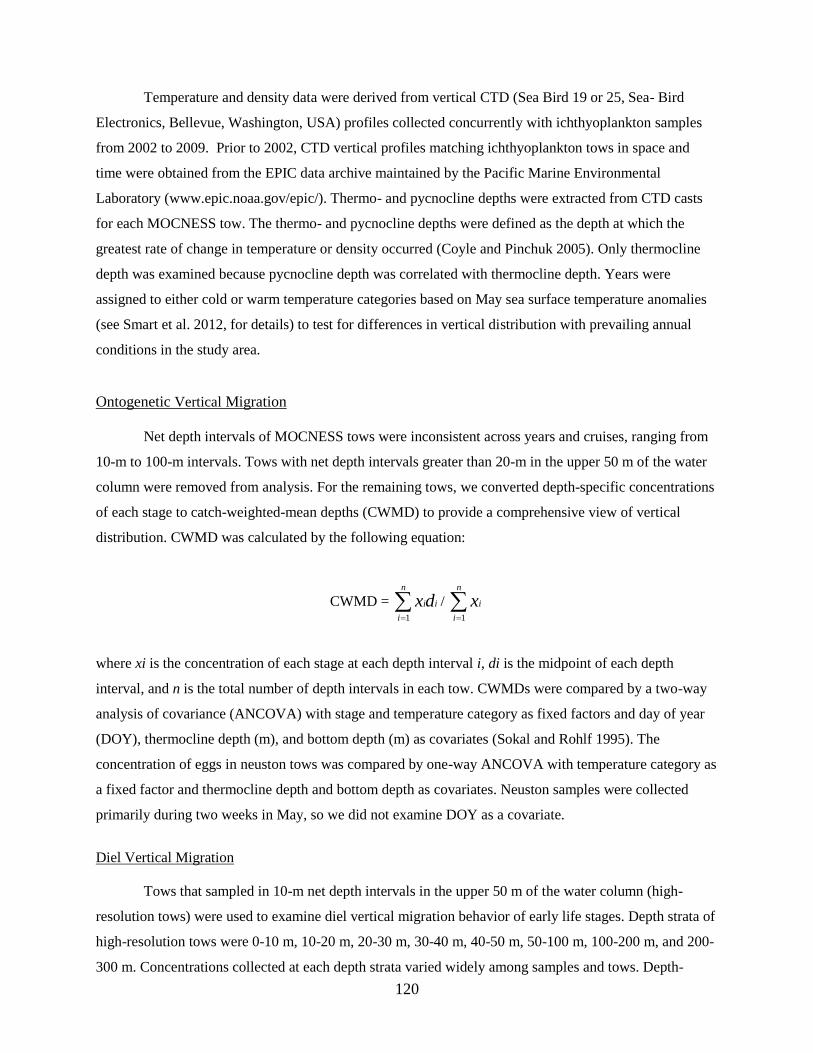
120
Temperature and density data were derived from vertical CTD (Sea Bird 19 or 25, Sea- Bird
Electronics, Bellevue, Washington, USA) profiles collected concurrently with ichthyoplankton samples
from 2002 to 2009. Prior to 2002, CTD vertical profiles matching ichthyoplankton tows in space and
time were obtained from the EPIC data archive maintained by the Pacific Marine Environmental
Laboratory (www.epic.noaa.gov/epic/). Thermo- and pycnocline depths were extracted from CTD casts
for each MOCNESS tow. The thermo- and pycnocline depths were defined as the depth at which the
greatest rate of change in temperature or density occurred (Coyle and Pinchuk 2005). Only thermocline
depth was examined because pycnocline depth was correlated with thermocline depth. Years were
assigned to either cold or warm temperature categories based on May sea surface temperature anomalies
(see Smart et al. 2012, for details) to test for differences in vertical distribution with prevailing annual
conditions in the study area.
Ontogenetic Vertical Migration
Net depth intervals of MOCNESS tows were inconsistent across years and cruises, ranging from
10-m to 100-m intervals. Tows with net depth intervals greater than 20-m in the upper 50 m of the water
column were removed from analysis. For the remaining tows, we converted depth-specific concentrations
of each stage to catch-weighted-mean depths (CWMD) to provide a comprehensive view of vertical
distribution. CWMD was calculated by the following equation:
CWMD = i
n
i
idx1
/
n
i
ix1
where xi is the concentration of each stage at each depth interval i, di is the midpoint of each depth
interval, and n is the total number of depth intervals in each tow. CWMDs were compared by a two-way
analysis of covariance (ANCOVA) with stage and temperature category as fixed factors and day of year
(DOY), thermocline depth (m), and bottom depth (m) as covariates (Sokal and Rohlf 1995). The
concentration of eggs in neuston tows was compared by one-way ANCOVA with temperature category as
a fixed factor and thermocline depth and bottom depth as covariates. Neuston samples were collected
primarily during two weeks in May, so we did not examine DOY as a covariate.
Diel Vertical Migration
Tows that sampled in 10-m net depth intervals in the upper 50 m of the water column (high-
resolution tows) were used to examine diel vertical migration behavior of early life stages. Depth strata of
high-resolution tows were 0-10 m, 10-20 m, 20-30 m, 30-40 m, 40-50 m, 50-100 m, 100-200 m, and 200-
300 m. Concentrations collected at each depth strata varied widely among samples and tows. Depth-
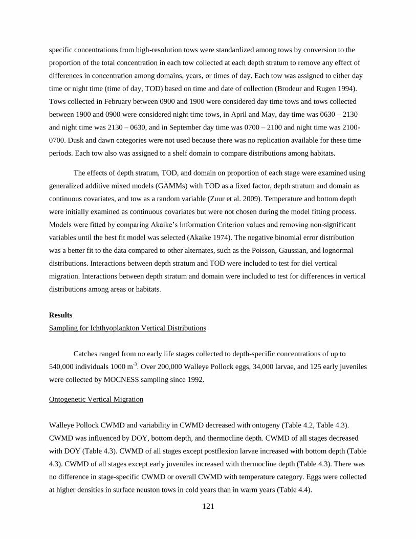
121
specific concentrations from high-resolution tows were standardized among tows by conversion to the
proportion of the total concentration in each tow collected at each depth stratum to remove any effect of
differences in concentration among domains, years, or times of day. Each tow was assigned to either day
time or night time (time of day, TOD) based on time and date of collection (Brodeur and Rugen 1994).
Tows collected in February between 0900 and 1900 were considered day time tows and tows collected
between 1900 and 0900 were considered night time tows, in April and May, day time was 0630 – 2130
and night time was 2130 – 0630, and in September day time was 0700 – 2100 and night time was 2100-
0700. Dusk and dawn categories were not used because there was no replication available for these time
periods. Each tow also was assigned to a shelf domain to compare distributions among habitats.
The effects of depth stratum, TOD, and domain on proportion of each stage were examined using
generalized additive mixed models (GAMMs) with TOD as a fixed factor, depth stratum and domain as
continuous covariates, and tow as a random variable (Zuur et al. 2009). Temperature and bottom depth
were initially examined as continuous covariates but were not chosen during the model fitting process.
Models were fitted by comparing Akaike’s Information Criterion values and removing non-significant
variables until the best fit model was selected (Akaike 1974). The negative binomial error distribution
was a better fit to the data compared to other alternates, such as the Poisson, Gaussian, and lognormal
distributions. Interactions between depth stratum and TOD were included to test for diel vertical
migration. Interactions between depth stratum and domain were included to test for differences in vertical
distributions among areas or habitats.
Results
Sampling for Ichthyoplankton Vertical Distributions
Catches ranged from no early life stages collected to depth-specific concentrations of up to
540,000 individuals 1000 m-3
. Over 200,000 Walleye Pollock eggs, 34,000 larvae, and 125 early juveniles
were collected by MOCNESS sampling since 1992.
Ontogenetic Vertical Migration
Walleye Pollock CWMD and variability in CWMD decreased with ontogeny (Table 4.2, Table 4.3).
CWMD was influenced by DOY, bottom depth, and thermocline depth. CWMD of all stages decreased
with DOY (Table 4.3). CWMD of all stages except postflexion larvae increased with bottom depth (Table
4.3). CWMD of all stages except early juveniles increased with thermocline depth (Table 4.3). There was
no difference in stage-specific CWMD or overall CWMD with temperature category. Eggs were collected
at higher densities in surface neuston tows in cold years than in warm years (Table 4.4).
122
Diel Vertical Migration
There was no evidence of DVM in Walleye Pollock eggs (Table 4.5, Figure 4.2), but the domain
in which they were collected interacted with the depth stratum in which proportion of total egg
concentration was highest (Table 4.5, Figure 4.3). Eggs were found ≤ 30 m in all three shelf domains but
≥ 100 m over the slope. Walleye Pollock eggs occurred throughout the water column, but proportion of
concentration was higher in the upper 20 m or below 100 m relative to the middle of the water column.
There was no difference in yolksac larval depth distribution between TODs (Table 4.5, Figure 4.4). There
were not enough replicate samples in multiple domains to assess for yolksac larvae. Yolksac larvae
occurred at depths less than 100 m, and proportion of concentration was highest from 10 – 40 m relative
to other depth strata.
For the two feeding larval stages, differences evidence for DVM were found. Preflexion larval
depth distribution differed between TODs although the level of significance was marginal (Table 4.5,
Figure 4.5). Overall, preflexion larvae were shallower and more concentrated in the day time than at night
time. Preflexion larvae were shallower over the shelf (10-20 m) than over the slope (20-30 m, Figure 4.6).
The interactions between depth strata and TOD were significant for postflexion larvae (Table 4.5).
Postflexion larvae exhibited regular DVM; deeper during the day (10 – 40 m) than at night (0 – 20 m,
Figure 4.7). Domain did not interact with depth stratum for postflexion larvae (Figure 4.8). Proportion of
postflexion larval concentration was highest above 30 m and lowest below 30 m relative to other strata.
Sample sizes for early juveniles were low relative to the other stages. Early juveniles tended to
occur deeper at night than during the day, but the interaction between TOD and depth strata was not
significant (Table 4.5, Figure 4.9). Early juvenile vertical distribution was not affected by domain (Figure
4.10). Early juveniles occurred at depths less than 100 m with greatest concentration from 0 to 20 m.
Discussion
Ontogenetic and diel vertical migrations have adaptive significance for planktonic organisms,
including optimal transport, energy conservation, access to prey, and avoidance of predators (Hunter and
Sanchez 1976, Fortier and Leggett 1983, Hare and Govoni 2005). For Walleye Pollock in the SEBS,
spawning occurs in either deep-water canyons or over the shelf, eggs are buoyant, and juveniles are
abundant over the shelf. Here, prey concentrations are highest in the upper water column and visual
predators occur in the water column and near the benthos. Based on these characteristics, we would
expect vertical migration strategies that maximize on-shelf transport from spawning grounds over the
basin or retention over the shelf, such as a decrease in depth of occurrence to provide access to prey and
123
minimize predation risk, such as OVM and regular DVM (Kerfoot 1985). For Walleye Pollock early life
stages in the SEBS, depth distribution became shallower and variability in depth distributions decreased
with ontogeny supporting OVM, similar to the GOA but unlike Funka Bay. Weighted mean depths
decreased with the progression of summer as stratification tended to increase. Weighted mean depths also
decreased as bottom depth decreased and as the thermocline depth decreased (except juveniles),
suggesting that distributions mirror the breadth of the available water column. Two of the five early life
stages examined exhibited evidence of DVM: reverse in preflexion larvae and regular in postflexion
larvae. These two stages are active feeders, while eggs and yolksac larvae are nonmotile or weak
swimmers and would not be expected to exhibit distribution patterns typically associated with active
behaviors. Sample sizes for early juveniles were too small to assess DVM adequately.
OVM in Walleye Pollock provides several advantages for the early life stages. First, the majority
of eggs over the slope were found deeper than 40 m, where they are exposed to the deep water Aleutian
North Slope Current through Bering Canyon or the Bering Slope Current through Pribilof Canyon. Eggs
spawned offshore, therefore, can be transported onto the shelf by these currents rather than advected
further over the Aleutian Basin by cyclonic flow above these currents (Reed and Stabeno 1999). Second,
high egg densities were observed in the neuston layer over the shelf in cold years when surface
temperatures were comparable to temperatures below in deep water in warm years (Stabeno et al. 2012),
allowing for extended development times and, by extension, the potential for increased time for on-shelf
transport in cold years, regardless of the vertical position. High egg densities in the surface layer in cold
years could be the result of a passive rise to the surface in the absence of a distinct density structure in the
water column or the result of delayed hatching at low temperatures. Third, yolksac larvae in the cooler
waters below 20 or 30 m depth will conserve energy and extend the period of time before yolk reserves
are exhausted and exogenous feeding must begin, which can be advantageous if larvae have not been
transported far enough over the shelf to where prey are available. Fourth, following the rise to the upper
20 m of the water column, feeding larvae have access to prey in the upper water column (Coyle and
Pinchuk 2005) and warmer water, both of which reduce development time.
DVM typically is exhibited by feeding stages reacting to changes in time of day and light
intensity, and Walleye Pollock conform to this pattern. As expected, neither eggs nor yolksac larvae
exhibited a pattern consistent with DVM. Vertical distributions of nonmotile or nonfeeding stages are
driven generally by physics such as buoyancy or passive mixing). These two early stages displayed
passive patterns which also suggests that diel differences in vertical distribution exhibited by feeding
stages was driven by behavior rather than by diel changes in the physical water column. In preliminary
analyses, we found no differences in the thermocline depth between day and night. Surprisingly, we were
124
unable to conclude that early juvenile Walleye Pollock undergo DVM, although they tended to be deeper
at night in the few tows in which they were collected. There is evidence from both laboratory (Sogard and
Olla 1996) and field (Bailey 1989) studies that vertical migration in shorter juveniles (< 60 mm) in the
GOA is weak and the migration to deeper layers intensifies as the fish gain locomotory and sensory
capabilities. Schabetsberger et al. (2000) documented DVM in juvenile Walleye Pollock between 30 and
92 mm SL near the Pribilof Islands. The juveniles in the present study were all shorter than 65 mm SL,
supporting that DVM in these shorter fish is weak in the SEBS and consistent with the previous findings
in the GOA. However, we were unable to address any impacts of predator presence or net avoidance in
the current study.
Walleye Pollock feeding larvae appear to take advantage of surface food concentrations, as they
primarily occurred shallower than 30 or 40 m at the onset of feeding. We did not have samples to
determine directly the vertical distributions of the preferred prey items, copepod eggs and nauplii.
Walleye Pollock undergo a transition from predominantly daytime feeding as larvae (Canino and Bailey
1995) to nocturnal feeding as juveniles (Brodeur et al. 2000). This is allowed by increased visual acuity
and sensitivity to light with ontogeny (Miller et al. 1993, Carvalho et al. 2004). Preflexion larval
distributions were consistent with reverse DVM (up during the day, down at night) and postflexion larvae
underwent regular DVM (down and variable during the day, up at night), suggesting that different trade-
offs between prey access, predator avoidance, and perhaps physical forces could be acting on the two
stages. Other studies have found that copepod nauplii do not undergo diel vertical migrations (Haldorson
et al. 1993, Irigoien et al. 2004). By moving into surface waters during the day when light levels are high
and where their preferred prey likely occur (Hillgruber et al. 1995, Brase 1996), preflexion larvae could
have higher success capturing prey since visual acuity is low relative to later stages. Postflexion larvae
would have higher capture success in surface waters at night at reduced light levels than preflexion larvae
because of their improved visual acuity. Postflexion larvae are large enough to be of interest to visual
predators such older age class Walleye Pollock (Juanes 2003), which could lead to the pattern of avoiding
surface waters during the day. Alternately, postflexion larvae in surface waters during the day may have
been better able to avoid our collection gears due to their visual acuity and swimming abilities.
Walleye Pollock vertical distributions vary among habitats both in the SEBS and the GOA.
Forward et al. (1996) found three different patterns of vertical distribution for Atlantic menhaden
(Brevoortia tyrannus) in three separate studies and suggested that vertical behaviors are flexible in order
to incorporate necessary trade-offs that vary between ecosystems or habitats. Eggs in the SEBS were
concentrated either below 100 m (slope) or in the upper 30 m (shelf domains), indicative of where they
were spawned and probably their buoyancy (Kendall and Nakatani 1992). SEBS yolksac larvae were
125
concentrated around 30 m. In the GOA, eggs are spawned at or below 150 m, followed by an increase in
depth prior to hatching (Kendall et al. 1994). GOA yolksac larvae remain at depths > 150 m for several
more days. One obvious difference between these systems is the depth of the water column and depth of
spawning activity. Olla et al. (1996) proposed that remaining at the spawning depth in the GOA provided
a predator refuge for eggs and yolksac larvae, an option that is not available in most of the SEBS habitats
due to their relatively shallow water column. SEBS preflexion larvae underwent reverse DVM in most
habitats and no DVM in the coastal domain. DVM is either regular or absent for preflexion larvae in the
GOA (Olla and Davis 1990 A, Davis and Olla 1994). In the shallow-water coastal domain, the stimulus to
move up during the day (e.g. sufficient light for hunting) may not be in place for SEBS preflexion larvae
because sufficient light levels are available throughout the shallow (≤ 50 m) water column (Kendall and
Nakatani 1992). Similar to larvae in the GOA, coastal domain SEBS preflexion larvae also could respond
to very high light levels at the surface during the day with negative phototaxis (Olla and Davis 1990 A).
Postflexion larvae in the SEBS undergo regular DVM, in accordance with behavior observed near Auke
Bay, Alaska, GOA (Haldorson et al. 1993). In Auke Bay, larvae migrated in response to the trade-off
between the vertical distribution of nauplii and avoidance of predators. For postflexion larvae, visual
predators occur in all areas in which this stage was collected and the same potential predators occur in the
SEBS, suggesting that the trade-off between feeding and predation risk could be a common factor across
habitats and ecosystems for this stage. We did not find support for DVM in SEBS early juveniles most
likely due to small sample sizes, but juveniles undergo regular DVM in the GOA (Olla and Davis 1990 B,
Brodeur and Rugen 1994) and larger juveniles near the Pribilof Islands in the SEBS undergo regular
DVM in response to prey movement (Schabetsberger et al. 2000).
Smart et al. (2012) found shifts in the spatial distributions of Walleye Pollock larvae and
juveniles between cold years and warm years. The authors hypothesized that spatial shifts were driven by
changes in area-specific mortality or transport. Satellite-tracked drifters and hydrographic models show
high variation in on- and off-shore transport among years (Danielson et al. 2011, Stabeno et al. 2012),
which could be linked to temperature conditions (Sohn et al. 2010) and might explain the differences in
spatial distribution. Annual differences in vertical distributions could impact the amount of transport off-
shore if larvae respond to variations in conditions with adjustments in their vertical distributions (Napp et
al. 2000). We found no support for differences in vertical distributions related to categorizing years as
either cold or warm.
Conclusions
126
Current speeds in the SEBS middle shelf tend to be slow relative to other spawning areas for
Walleye Pollock (< 5 cm s-1, Napp et al. 2000). Because of these slow speeds, the probability of retention
over the spawning grounds is high. Some off-shelf spawning grounds such as Bering Canyon may not
have the highest growth potential, thus selection for an ontogenetic migration toward the surface where
transport onto the shelf would be enhanced is likely in the SEBS. Walleye Pollock early life stages
underwent ontogenetic vertical migration and feeding stages were found in the upper portion of the water
column where prey availability is high typically. Feeding larvae also exhibited diel vertical migrations
that suggest trade-offs occurred between access to prey and exposure to predators. Characteristics of the
habitat and ecology of each stage suggested that some determinants of vertical distribution are common
between the SEBS and GOA (i.e. prey, light levels, predators) while others are not (i.e. depth refuges,
spawning depth). Several hypotheses developed for the SEBS have linked variation in recruitment to the
level of overlap between juveniles and their predators or juveniles and their prey, which in turn may be
related to the extent and direction of transport. For example, Wespestad et al. (2000) found that strong
year classes were linked to high spatial segregation of juveniles and cannibalistic older age classes. The
authors proposed that juvenile distribution was closely tied to the transport and distribution of eggs and
larvae. One way to address the connection between these various life stages is to model transport. Our
results clearly demonstrated that pollock larvae are not passive particles, early life stages are not
distributed randomly throughout the water column, and vertical distributions from the GOA are not
comparable to all stages in the SEBS. Accurate modeling needs to account for variation in vertical
distribution and behavior among stages and habitats, and these data are now available for the SEBS.
Acknowledgments
Thanks to the members of NOAA’s Ecosystems and Fisheries Oceanography Coordinated
Investigations (EcoFOCI) who were involved in the collection and processing of the ichthyoplankton
samples. This research was supported by the Bering Sea Integrated Ecosystem Research program
(BSIERP) of the North Pacific Research Board and the North Pacific Climate Regimes and Ecosystem
Productivity (NPCREP) program of the National Oceanographic and Atmospheric Administration. This
paper is EcoFOCI Contribution No. N754 – RAOA – N789, BEST-BSIERP Publication No. 89, and
NPRB Publication No. 407. We appreciate comments by Jeffrey Napp, Morgan Busby, Thomas Hurst,
and three anonymous reviewers.
127
Literature Cited
Akaike, H. 1974. A new look at the statistical model identification. IEEE Transactions on Automatic
Control 19, 716 – 723.
Bacheler, N.M., Ciannelli, L., Bailey, K.M., Duffy-Anderson, J.T., 2010. Spatial and temporal patterns of
Walleye Pollock spawning in the eastern Bering Sea inferred from egg and larval distributions.
Fish. Oceanogr. 19, 107 - 120.
Bailey, K.M., 1989. Interaction between the vertical distribution of juvenile Walleye Pollock Theragra
chalcogramma in the eastern Bering Sea and cannibalism. Mar. Ecol. Prog. Ser. 53, 205 – 213.
Brase, A.L.J., 1996. Temporal variation in feeding of larval Walleye Pollock (Theragra chalcogramma)
in the Southeastern Bering Sea shelf region. M.Sc. Thesis, Univ. Alaska, Fairbanks, AK.
Brodeur, R.D., Rugen, W.C., 1994. Diel vertical distribution of ichthyoplankton in the northern Gulf of
Alaska. Fish. Bull. 92, 223 – 235.
Brodeur, R.D., Wilson, M.T., 1996. A review of the distribution, ecology, and population dynamics of
age-0 Walleye Pollock in the Gulf of Alaska. Fish. Oceanogr. 5, 148 – 166.
Brodeur, R.D., Wilson, M.T., Ciannelli, L., 2000. Spatial and temporal variability in feeding and
condition of age-0 Walleye Pollock (Theragra chalcogramma) in frontal regions of the Bering
Sea. ICES J. Mar. Sci. 57, 256 – 264.
Canino, M.F., Bailey, K.M., 1995. Gut evacuation of Walleye Pollock larvae in response to feeding
conditions. J. Fish. Biol. 46, 389 – 403.
Carvalho, P.S.M., Noltie, D.B., Tillitt, D.E., 2004. Biochemical, histological and behavioural aspects of
visual function during early development of rainbow trout. J. Fish Biol. 64, 833 – 850.
Coachman, L.K., 1986. Circulation, water masses, and fluxes on the southeastern Bering Sea shelf. Cont.
Shelf Res. 5, 23-108.
Coyle, K.O., Pinchuk, A.I., 2005. Seasonal cross-shelf distribution of major zooplankton taxa on the
northern Gulf of Alaska shelf relative to water mass properties, species depth 414 preferences and
vertical migration behavior. Deep-Sea Res. II 52, 217 – 245.
Coyle, K.O., Eisner, L.B., Mueter, F.J., Pinchuk, A.I., Janout, M.A., Cieciel, K.D., Farley, E.V.,
Andrews, A.G., 2011. Climate change in the southeastern Bering Sea: impacts on pollock stocks
and implications for the oscillating control hypothesis. Fish. Oceanogr. 20, 139-418 156.
128
Danielson, S., Eisner, L., Weingartner, T., Aagaard, K., 2011. Thermal and haline variability over the
central Bering Sea shelf: Seasonal and interannual perspectives. Cont. Shelf 421 Res. 31, 539 –
554.
Davis, M.W., Olla, B.L., 1994. Ontogenetic shift in geotaxis for Walleye Pollock, Theragra
chalcogramma, free embryos and larvae: potential role in controlling vertical distribution.
Environ. Biol. Fishes 39, 313 – 318.
Duffy-Anderson, J.T., Ciannelli, L., Honkalehto, T., Bailey, K.M., Sogard, S.M., Springer, A.M., 426
Buckley, T., 2003. Distribution of age-1 and age-2 Walleye Pollock in the Gulf of Alaska and
eastern Bering Sea: sources of variation and implications for higher trophic levels. Institute of
Marine Research, Postboks 1870 Nordnes N-5817, Bergen Norway.
Fiksen, O., Jorgensen, C., Kristiansen, T., Vikebo, F., Huse, G., 2007. Linking behavioral ecology and
oceanography: larval behaviour determines growth, mortality and dispersal. Mar. Ecol. Prog. Ser.
347, 195 – 205.
Fortier, L., Leggett, W.C., 1983. Vertical migrations and transport of larval fish in a partially mixed
estuary. Can. J. Fish. Aquat. Sci. 40, 1543 – 1555.
Forward, R.B., Jr., Tankersley, R.A., Burke, J.S., 1996. Endogenous swimming rhythms of larval
Atlantic menhaden Brevoortia tyrannus Latrobe: Implications for vertical migration. J. Exp. Mar.
Biol. Ecol. 204, 195 – 207.
Haldorson, L., Prichett, M., Paul, A.J., Ziemann, D., 1993. Vertical distribution and migration of fish
larvae in a Northeast Pacific bay. Mar. Ecol. Prog. Ser. 101, 67 – 81.
Hare, J.A., Govoni, J.J., 2005. Comparison of average larval fish vertical distributions among species
exhibiting different transport pathways on the southeast United States continental shelf. Fish.
Bull. 103, 729 – 736.
Heath, M.R., Henderson, E.W., Baird, D.L., 1988. Vertical distribution of herring larvae in relation to
physical mixing and illumination. Mar. Ecol. Prog. Ser. 47, 211 – 228.
Hewitt, R.P., Methot, R.D., 1982. Distribution and mortality of northern anchovy larvae in 1978 and
1979. CalCOFI Report 23, 226 – 245.
Hillgruber, N., Haldorson, L.J., Paul, A.J., 1995. Feeding selectivity of larval Walleye Pollock 447
Theragra chalcogramma in the oceanic domain of the Bering Sea. Mar. Ecol. Prog. Ser. 448 120,
1 – 10.
129
Hinckley, S., 1987. The reproductive biology of Walleye Pollock, Theragra chalcogramma, in the Bering
Sea, with reference to spawning stock structure. Fish. Bull. 85, 481 - 498.
Hunt, G.L., Stabeno, P.J., Walters, G., Sinclair, E., Brodeur, R.D., Napp, J.M., Bond, N.A., 2002. Climate
change and control of the southeastern Bering Sea pelagic ecosystem. Deep-Sea Res. II 49, 5821 -
5853.
Hunter, J.R., Sanchez, C., 1976. Diel changes in swim bladder inflation of the larvae of the northern
anchovy Engraulis mordax. Fish. Bull. 74, 847 – 855.
Irigoien, X., Conway, D.V.P., Harris, R.P., 2004. Flexible diel vertical migration behaviour of
zooplankton in the Irish Sea. Mar. Ecol. Prog. Ser. 267, 85 – 97.
Joyeux, J.C., 1998. Spatial and temporal entry patterns of fish larvae into North Carolina estuaries:
comparisons among one pelagic and two demersal species. Est. Coast. Shelf Sci. 47, 731 – 752.
Juanes, F., 2003. The allometry of cannibalism in piscivorous fishes. Can. J. Fish. Aquat. Sci. 60, 594 –
602.
Kamba, M., 1977. Feeding habits and vertical distribution of Walleye Pollock, Theragra chalcogramma
(Pallas), in early life stage in Uchiura Bay, Hokkaido. Res. Inst. N. Pac. Fish., Hokkaido Univ.,
Spec. Vol., 175 – 197.
Kendall, A.W., Jr., Clarke, M.E., Yoklavich, M.M., Boehlert, G.W., 1987. Distribution, feeding, and
growth of larval Walleye Pollock, Theragra chalcogramma, from Shelikof Strait, Gulf of Alaska.
Fish. Bull. 85, 499 – 521.
Kendall, A.W., Jr., Incze, L.S., Ortner, P.B., Cummings, S.R., Brown, P.K., 1994. The vertical
distribution of eggs and larvae of Walleye Pollock (Theragra chalcogramma) in Shelikof Strait,
Gulf of Alaska. Fish. Bull. 92, 540 – 554.
Kerfoot, W.C., 1985. Adaptive value of vertical migration: Comments on the predation hypothesis and
some alternatives. Contrib. Mar. Sci. 27, 91–113.
Kristiansen, T., Joergensen, C., Lough, R.G., Vikeboe, F., Fiksen, O., 2009. Modeling rule- based
behavior: habitat selection and the growth-survival trade-off in larval cod. Behav. Ecol. 20, 490-
500.
130
Laurel, B.J., Stoner, A.W., Ryer, C.H., Hurst, T.P., Abookire, A.A., 2007. Comparative habitat
associations in juvenile Pacific Cod and other gadids using seines, baited cameras and laboratory
techniques. J. Exp. Mar. Biol. Ecol. 351, 42 – 55.
Matarese A.C., Blood, D.M., Picquelle, S.J., Benson, J.L., 2003. Atlas of abundance and distribution
patterns of ichthyoplankton from the northeast Pacific Ocean and Bering Sea ecosystems based
on research conducted by the Alaska Fisheries Science Center (1972-483 1996). NOAA Prof Pap
NMFS No. 1, NOAA, Seattle, WA.
Miller, T.J., Crowder, L.B., Rice, J.A., 1993. Ontogenetic changes in behavioural and histological
measures of visual acuity in three species of fish. Environ. Biol. Fish. 37, 1 –8.
Miller, T.J., 2007. Contribution of individual-based coupled physical-biological models to understanding
recruitment in marine fish populations. Mar. Ecol. Prog. Ser. 347, 127 –138.
Napp, J.M., Kendall, A.W., Shumacher, J.D., 2000. A synthesis of biological and physical processes
affecting the feeding environment of larval Walleye Pollock (Theragra chalcogramma) in the
eastern Bering Sea. Fish. Oceanogr. 9, 147 – 162.
Nishiyama, T., Hirano, K., Haryu, T., 1986. The early life history and feeding habits of larval Walleye
Pollock Theragra chalcogramma (Pallas) in the southeast Bering Sea. INPFC Bull. 45, 177-227.
Norcross, B.L., Shaw, R.F., 1984. Oceanic and estuarine transport of fish eggs and larvae: a review.
Trans. Am. Fish. Soc. 113, 153 – 165.
Ohman, M.D., 1990. The demographic benefits of diel vertical migration by zooplankton. Ecol. Monogr.
60, 257 – 281.
Olla, B.L., Davis, M.W., 1990 A. Effects of physical factors on the vertical distribution of larval Walleye
Pollock Theragra chalcogramma under controlled laboratory conditions. Mar. Ecol. Prog. Ser.
63, 105-122.
Olla, B.L., Davis, M.W., 1990 B. Behavioral responses of juvenile Walleye Pollock Theragra
chalcogramma Pallas to light, thermoclines and food: Possible role in vertical distribution. J. Exp.
Mar. Biol. Ecol. 135, 59 – 68.
Olla, B.L., Davis, M.W., Ryer, C.H., Sogard, S.M., 1996. Behavioural determinants of distribution and
survival in early stages of Walleye Pollock, Theragra chalcogramma: a synthesis of experimental
studies. Fish. Oceanogr. 5, 167-178.
131
Porter, S.M., Ciannelli, L., Hillgruber, N., Bailey, K.M., Chan, K.-S., Canino, M.F., Haldorson, L.J.,
2005. Environmental factors influencing larval Walleye Pollock Theragra chalcogramma feeding
in Alaskan waters. Mar. Ecol. Prog. Ser. 302, 207 - 217.
Reed R.K., Stabeno, P.J., 1999. The Aleutian North Slope Current. In: T.R. Loughlin and K. Ohtani
[eds.], Dynamics of the Bering Sea. University of Alaska Sea Grant, AK-SF-99-03, Fairbanks.
Schabetsberger, R., Brodeur, R.D., Ciannelli, L., Napp, J.M., Swartzman, G.L., 2000. Diel vertical
migration and interaction of zooplankton and juvenile Walleye Pollock (Theragra
chalcogramma) at a frontal region near the Pribilof Islands, Bering Sea. ICES J. Mar. Sci. 57,
1283 – 1295.
Serobaba, I.I., 1974. Spawning ecology of the Walleye Pollock, Theragra chalcogramma, in the Bering
Sea. J. Ichthyol. 14, 544 -552.
Shannon, L.V., Nelson, G., Crawford, R.J.M., Boyd, A.J., 1996. Possible impacts of environmental
change on pelagic fish recruitment: modeling anchovy transport by advective processes in the
southern Benguela. Global Change Biology 2, 407 – 420.
Shima M., Bailey, K.M., 1994. Comparative analysis of ichthyoplankton sampling gear for early life
stages of Walleye Pollock (Theragra chalcogramma). Fish. Oceanogr. 3, 50 - 59.
Smart T.I., Duffy-Anderson, J.T., Horne, J.K., Farley, E.V., Wilson, C.D., Napp, J.M., 2012. Influence of
environmental conditions on Walleye Pollock eggs, larvae, and juveniles in the southeastern
Bering Sea. Deep-Sea Res. II. 65 - 70, 196 – 207.
Smart T.I., Duffy-Anderson, J.T., Horne, J.K., 2012. Alternating temperature states influence Walleye
Pollock early life stages in the southeastern Bering Sea. Mar. Ecol. Prog. Ser. 455, 257 – 267.
Sogard S.M., Olla, B.L., 1996. Food deprivation affects vertical distribution and activity of a marine fish
in a thermal gradient: potential energy-conserving mechanisms. Mar. Ecol. Prog. Ser. 133, 43 –
55.
Sohn, D., Ciannelli, L., Duffy-Anderson, J.T., 2010. Distribution and drift pathways of Greenland halibut
(Reinhardtius hippoglossoides) during early life stages in the eastern Bering Sea and Aleutian
Islands. Fish. Oceanogr. 19, 339-353.
Sokal, R.R., Rohlf, F.J., 1995. Biometry: The Principles and Practice of Statistics in Biological Research.
W.H. Freemand and Co., New York.
132
Springer, A., McRoy, C.P., Flint, M., 1996. The Bering Sea Green Belt: shelf-edge processes and
ecosystem production. Fish. Oceanogr. 5, 205 – 223.
Stabeno, P.J., Bond, N.A., Kachel, N.B., Salo, S.A., Schumacher,.J.D., 2001. On the temporal variability
of the physical environment over the south-eastern Bering Sea. Fish. Oceanogr. 10, 81-98.
Stabeno P.J., Moore, S., Napp, J., Sigler, M., Zerbini, A., 2012. Comparison of warm and cold years on
the southeastern Bering Sea shelf and some implications for the ecosystem. Deep-Sea Res. II 65 –
70, 31 - 45.
Stenevik, E.K., Skogen, M., Sundby, S., Boyer, D., 2003. The effect of vertical and horizontal distribution
on retention of sardine (Sardinops sagax) larvae in the Northern Benguela –observations and
modelling. Fish. Oceanogr. 12, 185-200.
Tanaka, Y., 1991. Change of specific gravity of fish eggs and larvae and their distribution and movement
in relation to current structure, p. 60 – 78. In: E. Kawai [ed.], Current and life - Lecture of
fisheries oceanography. Kyoto University Press, Kyoto.
Walline, P.D., 1981. Hatching dates of Walleye Pollock (Theragra chalcogramma) and vertical
distribution of ichthyoplankton from the Eastern Bering Sea, June – July 1979. NWAFSC
Processed Report 81-05. NOAA Fisheries, Department of Commerce.
Wespestad, V.G., Fritz, L.W., Ingraham, W.J., Megrey, B.A., 2000. On relationships between
cannibalism, climate variability, physical transport, and recruitment success of Bering Sea
Walleye Pollock (Theragra chalcogramma). ICES J. Mar. Sci. 57, 268–274.
Wiebe, P.H., Burt, K.H., Boyd, S.H., Morton, A.W., 1976. A multiple opening/closing net and
environmental sensing system for sampling zooplankton. J. Mar. Res. 34, 313-326.
Yamashita, Y., Kitagawa, D., Aoyama, T., 1985. Diel vertical migration and feeding rhythm of the larvae
of the Japanese sand-eel Ammodytes personatus. Bull. Japan. Soc. Sci. Fish. 51, 1 – 5. Zuur, A.F.,
Ieno, E.N., Walker, N., Saveliev, A.A., Smith, G.M. 2009. Mixed Effects Models and Extensions
in Ecology with R. Springer, New York, NY. 574 p.
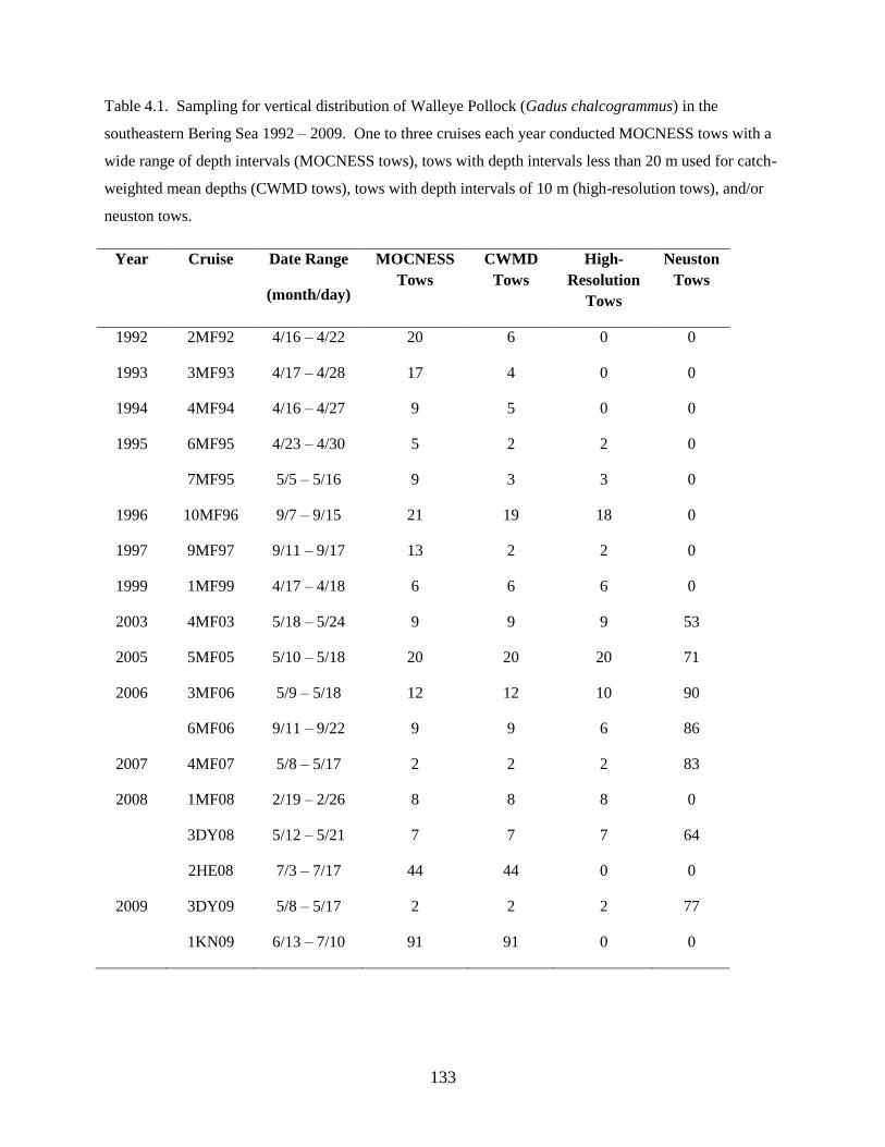
133
Table 4.1. Sampling for vertical distribution of Walleye Pollock (Gadus chalcogrammus) in the
southeastern Bering Sea 1992 – 2009. One to three cruises each year conducted MOCNESS tows with a
wide range of depth intervals (MOCNESS tows), tows with depth intervals less than 20 m used for catch-
weighted mean depths (CWMD tows), tows with depth intervals of 10 m (high-resolution tows), and/or
neuston tows.
Year Cruise Date Range
(month/day)
MOCNESS
Tows
CWMD
Tows
High-
Resolution
Tows
Neuston
Tows
1992 2MF92 4/16 – 4/22 20 6 0 0
1993 3MF93 4/17 – 4/28 17 4 0 0
1994 4MF94 4/16 – 4/27 9 5 0 0
1995 6MF95 4/23 – 4/30 5 2 2 0
7MF95 5/5 – 5/16 9 3 3 0
1996 10MF96 9/7 – 9/15 21 19 18 0
1997 9MF97 9/11 – 9/17 13 2 2 0
1999 1MF99 4/17 – 4/18 6 6 6 0
2003 4MF03 5/18 – 5/24 9 9 9 53
2005 5MF05 5/10 – 5/18 20 20 20 71
2006 3MF06 5/9 – 5/18 12 12 10 90
6MF06 9/11 – 9/22 9 9 6 86
2007 4MF07 5/8 – 5/17 2 2 2 83
2008 1MF08 2/19 – 2/26 8 8 8 0
3DY08 5/12 – 5/21 7 7 7 64
2HE08 7/3 – 7/17 44 44 0 0
2009 3DY09 5/8 – 5/17 2 2 2 77
1KN09 6/13 – 7/10 91 91 0 0
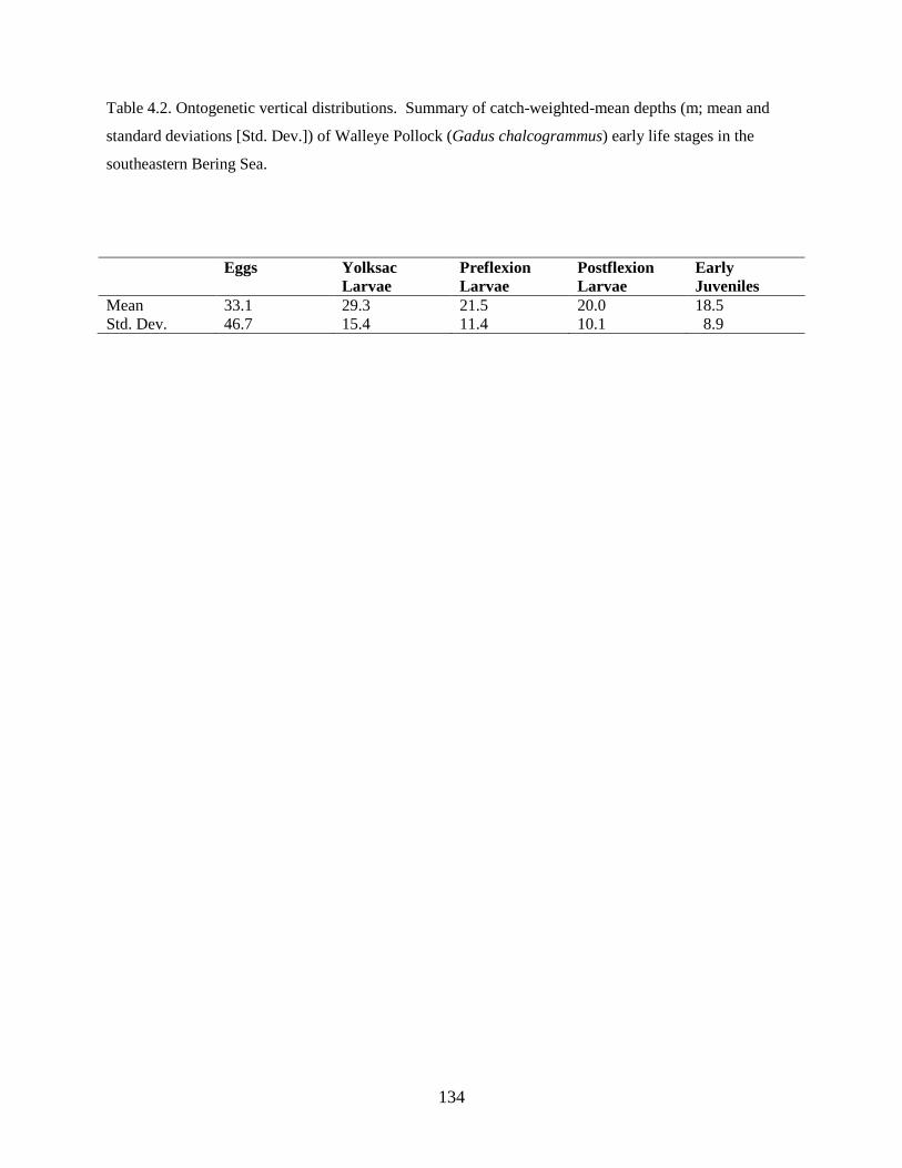
134
Table 4.2. Ontogenetic vertical distributions. Summary of catch-weighted-mean depths (m; mean and
standard deviations [Std. Dev.]) of Walleye Pollock (Gadus chalcogrammus) early life stages in the
southeastern Bering Sea.
Eggs Yolksac
Larvae
Preflexion
Larvae
Postflexion
Larvae
Early
Juveniles
Mean 33.1 29.3 21.5 20.0 18.5
Std. Dev. 46.7 15.4 11.4 10.1 8.9
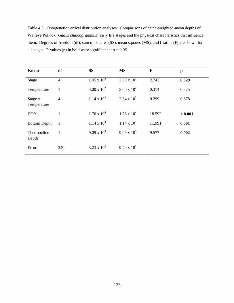
135
Table 4.3. Ontogenetic vertical distribution analyses. Comparisons of catch-weighted-mean depths of
Walleye Pollock (Gadus chalcogrammus) early life stages and the physical characteristics that influence
them. Degrees of freedom (df), sum of squares (SS), mean squares (MS), and f-ratios (F) are shown for
all stages. P-values (p) in bold were significant at α = 0.05.
Factor df SS MS F p
Stage 4 1.05 x 10⁴ 2.60 x 10
3 2.743 0.029
Temperature 1 3.00 x 10² 3.00 x 10
2 0.314 0.575
Stage x
Temperature
4 1.14 x 10³ 2.84 x 10
2 0.299 0.878
DOY 1 1.76 x 10⁴ 1.76 x 10
4 18.592 < 0.001
Bottom Depth 1 1.14 x 10⁴ 1.14 x 10
4 11.991 0.001
Thermocline
Depth
1 9.09 x 10³ 9.09 x 10
3 9.577 0.002
Error 340 3.23 x 10⁵ 9.49 x 10
2
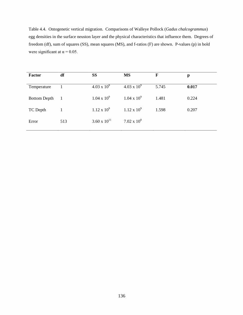
136
Table 4.4. Ontogenetic vertical migration. Comparisons of Walleye Pollock (Gadus chalcogrammus)
egg densities in the surface neuston layer and the physical characteristics that influence them. Degrees of
freedom (df), sum of squares (SS), mean squares (MS), and f-ratios (F) are shown. P-values (p) in bold
were significant at α = 0.05.
Factor df SS MS F p
Temperature 1 4.03 x 10⁹ 4.03 x 10
9 5.745 0.017
Bottom Depth 1 1.04 x 10⁹ 1.04 x 10
9 1.481 0.224
TC Depth 1 1.12 x 10⁹ 1.12 x 10
9 1.598 0.207
Error 513 3.60 x 10¹¹
7.02 x 10⁸
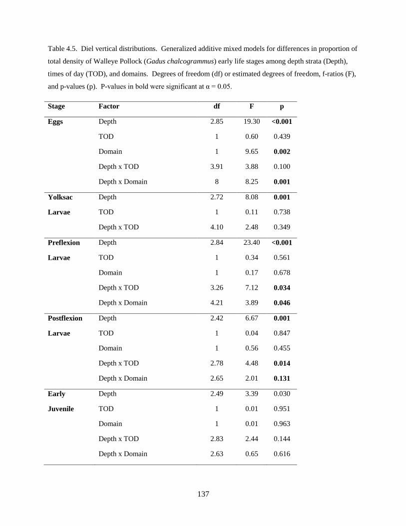
137
Table 4.5. Diel vertical distributions. Generalized additive mixed models for differences in proportion of
total density of Walleye Pollock (Gadus chalcogrammus) early life stages among depth strata (Depth),
times of day (TOD), and domains. Degrees of freedom (df) or estimated degrees of freedom, f-ratios (F),
and p-values (p). P-values in bold were significant at α = 0.05.
Stage Factor df F p
Eggs Depth 2.85 19.30 <0.001
TOD 1 0.60 0.439
Domain 1 9.65 0.002
Depth x TOD 3.91 3.88 0.100
Depth x Domain 8 8.25 0.001
Yolksac Depth 2.72 8.08 0.001
Larvae TOD 1 0.11 0.738
Depth x TOD 4.10 2.48 0.349
Preflexion Depth 2.84 23.40 <0.001
Larvae TOD 1 0.34 0.561
Domain 1 0.17 0.678
Depth x TOD 3.26 7.12 0.034
Depth x Domain 4.21 3.89 0.046
Postflexion Depth 2.42 6.67 0.001
Larvae TOD 1 0.04 0.847
Domain 1 0.56 0.455
Depth x TOD 2.78 4.48 0.014
Depth x Domain 2.65 2.01 0.131
Early Depth 2.49 3.39 0.030
Juvenile TOD 1 0.01 0.951
Domain 1 0.01 0.963
Depth x TOD 2.83 2.44 0.144
Depth x Domain 2.63 0.65 0.616
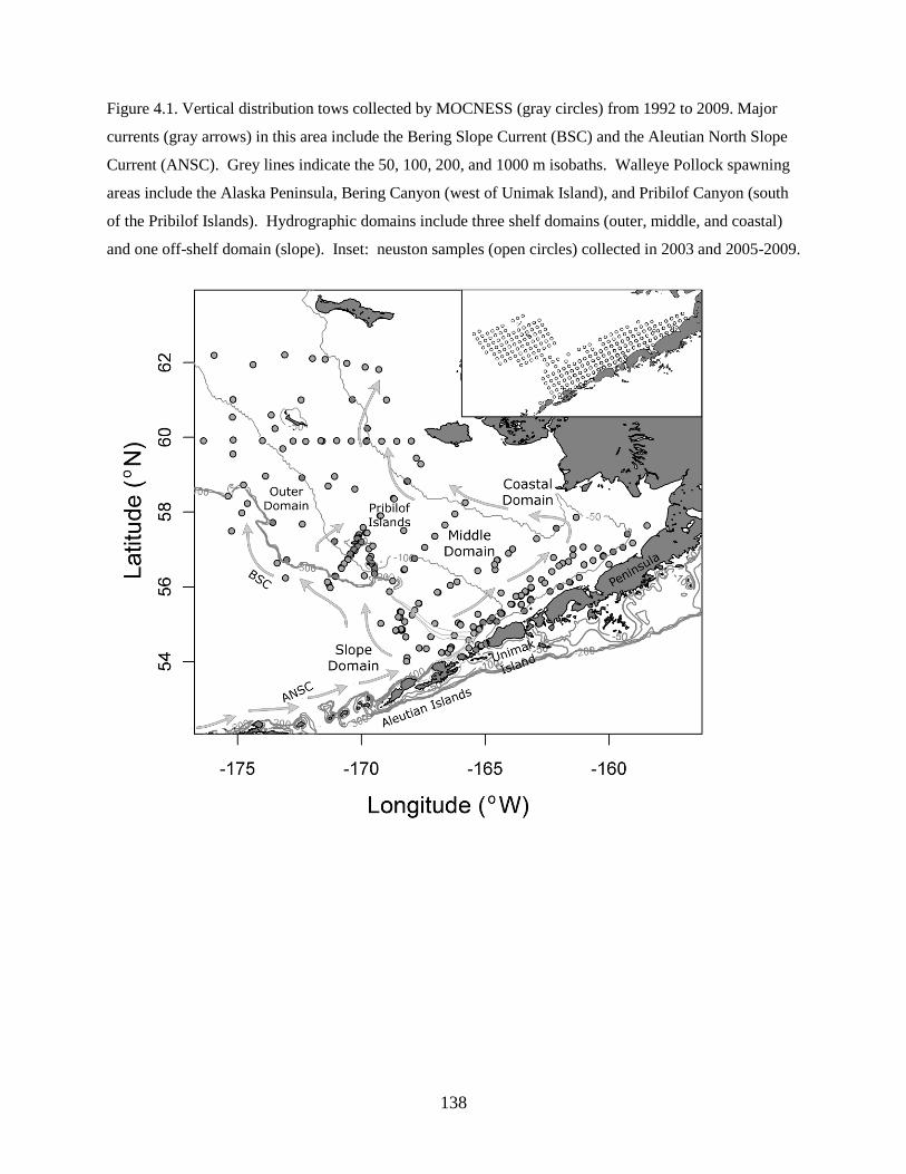
138
Figure 4.1. Vertical distribution tows collected by MOCNESS (gray circles) from 1992 to 2009. Major
currents (gray arrows) in this area include the Bering Slope Current (BSC) and the Aleutian North Slope
Current (ANSC). Grey lines indicate the 50, 100, 200, and 1000 m isobaths. Walleye Pollock spawning
areas include the Alaska Peninsula, Bering Canyon (west of Unimak Island), and Pribilof Canyon (south
of the Pribilof Islands). Hydrographic domains include three shelf domains (outer, middle, and coastal)
and one off-shelf domain (slope). Inset: neuston samples (open circles) collected in 2003 and 2005-2009.
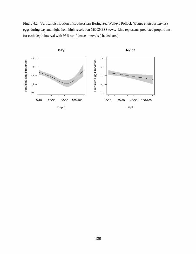
139
Figure 4.2. Vertical distribution of southeastern Bering Sea Walleye Pollock (Gadus chalcogrammus)
eggs during day and night from high-resolution MOCNESS tows. Line represents predicted proportions
for each depth interval with 95% confidence intervals (shaded area).
-2-1
01
2
Day
Depth
Pre
dic
ted
Eg
g P
rop
ort
ion
0-10 20-30 40-50 100-200-2
-10
12
Night
Depth
Pre
dic
ted
Eg
g P
rop
ort
ion
0-10 20-30 40-50 100-200
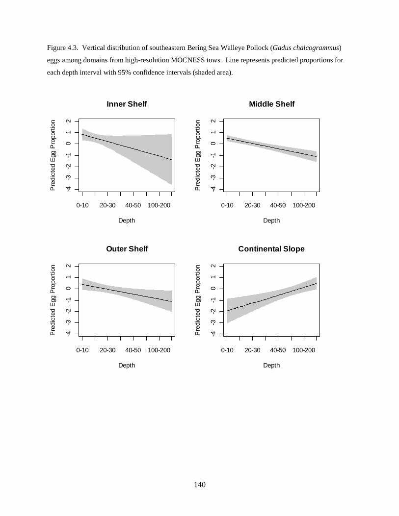
140
Figure 4.3. Vertical distribution of southeastern Bering Sea Walleye Pollock (Gadus chalcogrammus)
eggs among domains from high-resolution MOCNESS tows. Line represents predicted proportions for
each depth interval with 95% confidence intervals (shaded area).
-4-3
-2-1
01
2
Inner Shelf
Depth
Pre
dic
ted E
gg P
roport
ion
0-10 20-30 40-50 100-200-4
-3-2
-10
12
Middle Shelf
Depth
Pre
dic
ted E
gg P
roport
ion
0-10 20-30 40-50 100-200
-4-3
-2-1
01
2
Outer Shelf
Depth
Pre
dic
ted E
gg P
roport
ion
0-10 20-30 40-50 100-200
-4-3
-2-1
01
2
Continental Slope
Depth
Pre
dic
ted E
gg P
roport
ion
0-10 20-30 40-50 100-200
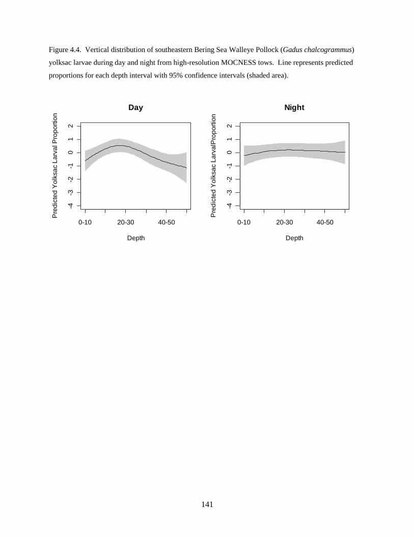
141
Figure 4.4. Vertical distribution of southeastern Bering Sea Walleye Pollock (Gadus chalcogrammus)
yolksac larvae during day and night from high-resolution MOCNESS tows. Line represents predicted
proportions for each depth interval with 95% confidence intervals (shaded area).
-4-3
-2-1
01
2
Day
Depth
Pre
dic
ted
Yo
lksa
c L
arv
al P
rop
ort
ion
0-10 20-30 40-50-4
-3-2
-10
12
Night
Depth
Pre
dic
ted
Yo
lksa
c L
arv
alP
rop
ort
ion
0-10 20-30 40-50
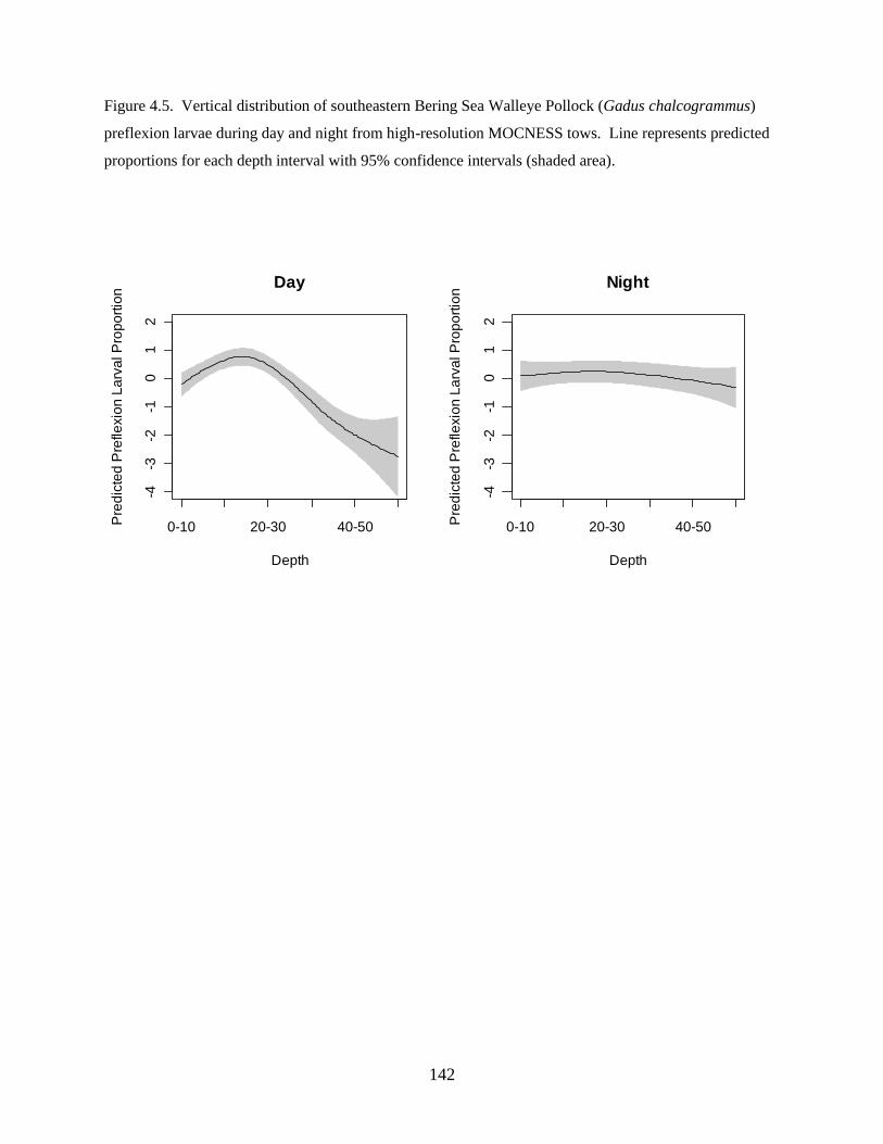
142
Figure 4.5. Vertical distribution of southeastern Bering Sea Walleye Pollock (Gadus chalcogrammus)
preflexion larvae during day and night from high-resolution MOCNESS tows. Line represents predicted
proportions for each depth interval with 95% confidence intervals (shaded area).
-4-3
-2-1
01
2
Day
Depth
Pre
dic
ted
Pre
fle
xio
n L
arv
al P
rop
ort
ion
0-10 20-30 40-50
-4-3
-2-1
01
2
Night
Depth
Pre
dic
ted
Pre
fle
xio
n L
arv
al P
rop
ort
ion
0-10 20-30 40-50
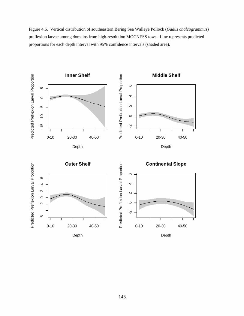
143
Figure 4.6. Vertical distribution of southeastern Bering Sea Walleye Pollock (Gadus chalcogrammus)
preflexion larvae among domains from high-resolution MOCNESS tows. Line represents predicted
proportions for each depth interval with 95% confidence intervals (shaded area).
-15
-10
-50
5
Inner Shelf
Depth
Pre
dic
ted P
reflexio
n L
arv
al P
roport
ion
0-10 20-30 40-50
-20
24
6
Middle Shelf
Depth
Pre
dic
ted P
reflexio
n L
arv
al P
roport
ion
0-10 20-30 40-50
-6-2
02
46
Outer Shelf
Depth
Pre
dic
ted P
reflexio
n L
arv
al P
roport
ion
0-10 20-30 40-50
-20
24
6
Continental Slope
Depth
Pre
dic
ted P
reflexio
n L
arv
al P
roport
ion
0-10 20-30 40-50
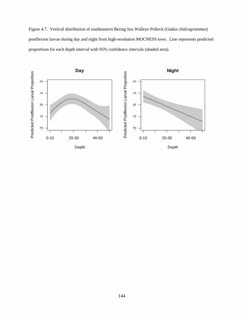
144
Figure 4.7. Vertical distribution of southeastern Bering Sea Walleye Pollock (Gadus chalcogrammus)
postflexion larvae during day and night from high-resolution MOCNESS tows. Line represents predicted
proportions for each depth interval with 95% confidence intervals (shaded area).
-2-1
01
2
Day
Depth
Pre
dic
ted
Po
stfle
xio
n L
arv
al P
rop
ort
ion
0-10 20-30 40-50-2
-10
12
Night
Depth
Pre
dic
ted
Po
stfle
xio
n L
arv
al P
rop
ort
ion
0-10 20-30 40-50
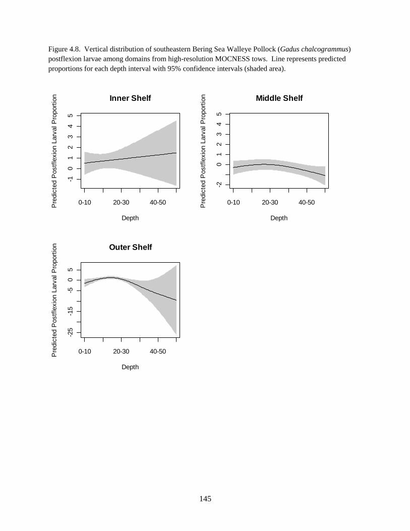
145
Figure 4.8. Vertical distribution of southeastern Bering Sea Walleye Pollock (Gadus chalcogrammus)
postflexion larvae among domains from high-resolution MOCNESS tows. Line represents predicted
proportions for each depth interval with 95% confidence intervals (shaded area).
-10
12
34
5
Inner Shelf
Depth
Pre
dic
ted P
ostf
lexio
n L
arv
al P
roport
ion
0-10 20-30 40-50
-20
12
34
5
Middle Shelf
Depth
Pre
dic
ted P
ostf
lexio
n L
arv
al P
roport
ion
0-10 20-30 40-50
-25
-15
-50
5
Outer Shelf
Depth
Pre
dic
ted P
ostf
lexio
n L
arv
al P
roport
ion
0-10 20-30 40-50
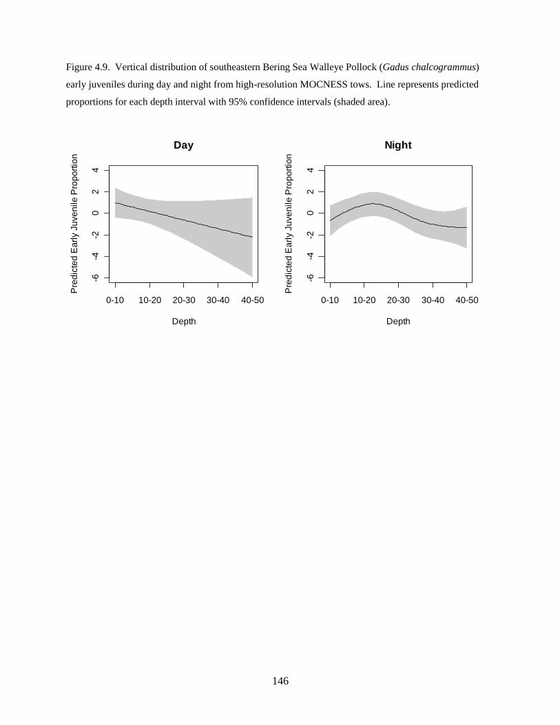
146
Figure 4.9. Vertical distribution of southeastern Bering Sea Walleye Pollock (Gadus chalcogrammus)
early juveniles during day and night from high-resolution MOCNESS tows. Line represents predicted
proportions for each depth interval with 95% confidence intervals (shaded area).
-6-4
-20
24
Day
Depth
Pre
dic
ted
Ea
rly J
uve
nile
Pro
po
rtio
n
0-10 10-20 20-30 30-40 40-50-6
-4-2
02
4
Night
Depth
Pre
dic
ted
Ea
rly J
uve
nile
Pro
po
rtio
n
0-10 10-20 20-30 30-40 40-50
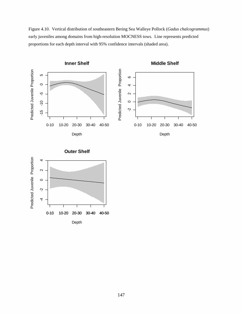
147
Figure 4.10. Vertical distribution of southeastern Bering Sea Walleye Pollock (Gadus chalcogrammus)
early juveniles among domains from high-resolution MOCNESS tows. Line represents predicted
proportions for each depth interval with 95% confidence intervals (shaded area).
-15
-10
-50
5
Inner Shelf
Depth
Pre
dic
ted J
uvenile
Pro
port
ion
0-10 10-20 20-30 30-40 40-50-2
02
46
Middle Shelf
Depth
Pre
dic
ted J
uvenile
P
roport
ion
0-10 10-20 20-30 30-40 40-50
-4-2
02
4
Outer Shelf
Depth
Pre
dic
ted J
uvenile
P
roport
ion
0-10 10-20 20-30 30-40 40-500-10 10-20 20-30 30-40 40-50
148
Chapter 5: Biophysical transport model suggests climate variability determines distribution of
Walleye Pollock early life stages in the Eastern Bering Sea through effects on spawning
Colleen M. Petrik1,2
, Janet T. Duffy-Anderson3, Franz Mueter
1, Katherine Hedstrom
4, and
Enrique N. Curchitser5
1University of Alaska Fairbanks, School of Fisheries and Ocean Sciences, 17101 Point Lena
Loop Rd., Juneau, AK 99801, USA
2Present address: UC Santa Cruz, Institute of Marine Sciences, 110 Shaffer Rd., Santa Cruz, CA 95060,
USA
3Alaska Fisheries Science Center, NOAA NMFS, 7600 Sand Point Way NE, Seattle, WA 98115,
USA
4Univeristy of Alaska Fairbanks, Arctic Region Supercomputing Center, 105 West Ridge Research Bldg.,
P.O. Box 756020, Fairbanks, AK 99775, USA
5Department of Environmental Sciences and Institute of Marine and Coastal Sciences, Rutgers
University, 14 College Farm Rd., New Brunswick, NJ 08901, USA
Citation: Petrik, C., Duffy-Anderson, J.T., Mueter, F.J., Hedstrom, K., and Curchitser, E. In press.
Modeling the effect of climate variations on the transport and distribution of Walleye Pollock early life
stages in the eastern Bering Sea. Progress in Oceanography.
http://www.sciencedirect.com/science/article/pii/S0079661114001128
149
Abstract
The eastern Bering Sea recently experienced an anomalously warm period followed by an anomalously
cold period. These periods varied with respect to sea ice extent, water temperature, wind patterns, and
ocean circulation. The distributions of Walleye Pollock early life stages also differed between periods,
with stages found further eastward on the shelf in warm years. Statistical analyses indicated that these
spatial distributions were more closely related to temperature than to other covariates, though a
mechanism has not been identified. The objective of this study was to determine if variable transport
could be driving the observed differences in pollock distributions. An individual-based model of pollock
early life stages was developed by coupling a hydrodynamic model to a particle-tracking model with
biology and behavior. Simulation experiments were performed with the model to investigate the effect of
wind on transport, ice presence on time of spawning, and water temperature on location of spawning.
This modeling approach benefited from the ability to individually test mechanisms to quantitatively
assess the impact of each on the distribution of pollock. Neither interannual variations in advection nor
advances or delays in spawning time could adequately represent the observed differences in distribution
between warm and cold years. Changes to spawning areas, particularly spatial contractions of spawning
areas in cold years, resulted in modeled distributions that were most similar to observations. The location
of spawning pollock in reference to cross-shelf circulation patterns is important in determining the
distribution of eggs and larvae, warranting further study on the relationship between spawning adults and
the physical environment. The different distributions of pollock early life stages between warm and cold
years may ultimately affect recruitment by influencing the spatial overlap of pollock juveniles with prey
and predators.
150
Introduction
The eastern Bering Sea shelf is one of the most biologically productive marine ecosystems in the
world with marine resources that are integral to the culture and diet of native Alaskans and that comprise
roughly 50% of the US commercial fish harvest. The continental shelf extends approximately 500 km
westward from the Alaskan mainland coast to the Aleutian Basin shelfbreak and 1000 km northward from
the Alaska Peninsula to the Bering Strait. The shelf can be divided into three regions based on
bathymetry: inner shelf (<50 m), middle shelf (50-100 m), and outer shelf (>100 m; Coachman 1986).
The inner shelf is weakly stratified and influenced by freshwater runoff, while the middle and outer
shelves are strongly stratified (Coachman 1986). A large and highly variable portion of the shelf is ice-
covered during winter, cooling the entire water column and resulting in a bottom layer of very cold water
over much of the middle shelf that persists through the summer (the “cold pool”). Offshore, the Bering
Slope Current (Figure 5.1) transports nutrient-rich waters along the slope to the northwest, replenishing
nutrients on the shelf through cross-shelf exchanges associated with eddies (Mizobata et al. 2008),
intrusions of water in canyons (Stabeno et al. 2008), and wind-forced cross-shelf flows (Stabeno et al.
2001, Danielson et al. 2011). Mean circulation over the shelf is dominated by the Alaska Coastal Current,
which is a seasonal current that flows roughly parallel to the 50-m isobath northeast along the Alaska
Peninsula, around Bristol Bay, and continues to the northwest off of mainland Alaska towards the Bering
Strait (Figure 5.1). Cross-shelf and along-shelf flows provide important pathways for the planktonic
stages of many species that spawn on the outer shelf or slope to reach suitable nursery areas (Lanksbury et
al. 2007, Wespestad et al. 2000, Wilderbuer et al. 2013).
Walleye Pollock (Gadus chalcogrammus; hereafter pollock) is an ecologically and commercially
important gadid in the eastern Bering Sea, supporting one of the largest single-species fisheries in the
world. Adults are semi-demersal and occur primarily in regions 50-300 m deep (Duffy-Anderson et al. in
review). Females are iterative spawners with up to 10 batches per female per year (Duffy-Anderson et al.
in review). Pollock show fidelity to at least two spawning sites over the southeastern Bering Sea shelf
(Figure 5.1). Spawning begins nearshore north of Unimak Island in March and April and later near the
Pribilof Islands from April through August (Jung et al. 2006, Bacheler et al. 2010). Egg production from
these two locations peaks in April or May (Bacheler et al. 2010). Eggs can be found as deep as 300 m, but
the center of the vertical distribution is < 30 m (Smart et al. 2012). Egg incubation lasts 18-34 days and
yolksac larvae hatch at 4.6-5.7 mm standard length (SL), both depending on temperature (Blood 2002).
Larvae develop in the upper 100 m of the water column and the depth of maximum abundance shifts
deeper with age. Depth differences are related to flexion, which occurs between 10 and 17 mm SL, after
which larval swimming ability increases (Dunn & Matarese 1987). Pollock transition from larva to
151
pelagic juvenile when they are 30-40 mm SL (Matarese et al. 1989) at age-0 and recruit into the fishery at
age-3 to age-4 (Ianelli et al. 2012a).
The eastern Bering Sea recently experienced a prolonged warm period (2001-2005), followed by
a prolonged cold period (2007-2012; Stabeno et al. 2012). During colder than average years, winter ice
extends farther south and offshore, creating a cold pool of bottom water <2○C that influences the
distribution (Mueter & Litzow 2008, Barbeaux 2012, Ianelli et al. 2012a) and potentially the spawning
ecology of pollock and other demersal fishes. The timing and location of pollock spawning affect the
initial distribution of eggs, while their subsequent advection is a function of prevailing atmospheric and
hydrographic conditions. Therefore both the initial distribution and advective forcing vary from year to
year due to climatic variability. For example, strong northward flow and/or weaker cross-shelf flow have
been observed at a hydrographic mooring over the middle shelf during the recent warm period compared
to recent cold years that had strong westward flow (Stabeno et al. 2012), which could affect the dispersal
of pelagic early life stages (ELS). Modeling results suggest generally enhanced on-shelf transport when
winds blow predominantly from the southeast during winter (Danielson et al. 2011), which coincided
with warm temperatures from 2001 to 2005, while the following cold years were characterized by winds
from the northwest. It has been speculated that these differences in advection influence the distributions
of pollock ELS, whose centers are further inshore in warm years than cold years (Smart et al. 2012).
The observed variability in distribution could be the result of differences in physical transport as
hypothesized, or they could be the result of biological responses to physical variation. Preliminary
analysis of roe fishery harvest data and pollock fishery observer maturity data suggest that spawning
extends further onshore in warm years (S. Barbeaux unpub. data) and is delayed in time by as much as 40
d in cold years (Jung et al. 2006, Smart et al. 2012). Differences in water temperature could not only
impact where adults spawn, but also the development rates of ELS.
Mechanisms behind the distribution differences have not been identified, and effects of climate
variation on the dispersal of pollock ELS are poorly understood. In order to gain a clearer understanding
of the forcing mechanisms that underlie observed spatial differences in pollock egg and larval
distribution, we developed an individual-based model of pollock biology and behavior (TRACMASS)
coupled to a hydrodynamic model (ROMS). Our objective was to test the effects of atmospheric (wind),
oceanographic (ice, water column temperature), and biological (time and location of spawning) conditions
on the distribution, development, and transport of Walleye Pollock eggs and larvae. Model results are
used to elucidate the dominant physical mechanisms responsible for observed changes. We present a
152
description of the coupled biophysical model, its validation with observations, and its use to evaluate
mechanisms that determine the spatial distribution of propagules during warm and cold years.
Methods
Observational data
Ichthyoplankton surveys
Observational data from the Fisheries Oceanographic Coordinated Investigations (FOCI) surveys
and Bering Ecosystem Study and Bering Sea Integrated Ecosystem Research Project (BEST-BSIERP)
cruises were used for model-data comparisons. Observational data included egg and larval samples
collected with Bongo nets, Multiple Opening/Closing Net and Environmental Sensing System
(MOCNESS), Modified Bottom Trawls (MBTs), and Tucker trawls. Larval stages were segregated by
length: yolksac < 6 mm; 6 mm ≤ preflexion < 10 mm; 10 mm ≤ late < 40 mm (Matarese et al. 1989). Data
from all four gear types were used to characterize horizontal distributions, while only depth-stratified
MOCNESS samples were used for the vertical distributions since the other gear types did not provide
enough vertical resolution. Horizontal distributions were determined for each stage and for each available
month and year from 1995 to 2012, by aggregating all observations within a given month and year. To
quantify horizontal distributions, vertically integrated concentrations (number per 10 m2) were computed
over the entire depth range sampled by depth-stratified tows (MOCNESS, MBT, Tucker) so that they
were comparable to non-stratified samples (Bongo). All available data sets from 1995 and 2007 were used
for model selection. Only data from the cruises listed in Smart et al. (2012) were used for comparison
between observed and modeled distributions in warm and cold years.
Spawning data
Two different data sets were used to provide information on potential locations for initializing
particles as eggs in the model. The first data set was derived from collections of female pollock for the roe
fishery (S. Barbeaux unpub. data). These data included the day of fishing, the centroid latitude and
longitude of where the boat was fishing that day, and the amount of roe of each quality caught that day for
the years 2001-2006. The market quality of roe deteriorates as the adults near spawning and is ranked as
immature, mature, overmature, or other. Hydrated roe is within a few days of spawning and of the worst
quality (S. Barbeaux pers. comm.). We used only presence and absence data of the hydrated, overmature
roe as a proxy for spawning times and locations.
The second data set consisted of maturity index classifications from the NOAA Fisheries North
Pacific groundfish observer program. These data were obtained on pollock fillet fishery vessels from
153
2008-2012 and contained date, latitude, longitude, bottom depth, fishing depth, and a maturity index.
Observers classify the maturity level of a random subsample of the catch using the maturity indices:
immature, developing, pre-spawn, spawning, and spent. We used only the dates and locations where
female pollock in spawning condition were recorded as a proxy for spawning times and locations.
These data were used together with available literature on dominant spawning areas (Bacheler et
al. 2010, Hinckley 1987) to infer generalized spawning distributions for warm and cold years,
respectively, as described below. We were unable to use annual observations on spawning times and
locations for model initialization because neither data set spanned the whole time period of interest from
2000 to 2012. Furthermore, the two data sets could not be combined because they used data from
different fisheries and used different classification methods.
Physical model
We used an implementation of the Regional Ocean Modeling System (ROMS; Shchepetkin &
McWilliams 2009) as the hydrodynamic model to force the Lagrangian particle-tracking model. ROMS is
a free-surface, hydrostatic primitive equation ocean circulation model. It is a terrain-following, finite
volume (Arakawa C-grid) model with the following advanced features: high-order, weakly dissipative
algorithms for tracer advection; a unified treatment of surface and bottom boundary layers (e.g., K-Profile
Parameterization; Large et al. 1994); atmosphere-ocean flux computations based on the ocean model
prognostic variables using bulk-formulae. ROMS has been coupled to a sea-ice model (Budgell 2005)
consisting of the elastic-viscous-plastic (EVP) rheology (Hunke & Dukowicz 1997) and the Mellor and
Kantha (1989) thermodynamics. The sea ice code is fully explicit and implemented on the ROMS
Arakawa C-grid and is therefore fully parallel, just as ROMS is. The model also includes frazil ice growth
in the ocean being passed to the ice (Steele et al. 2004). It currently follows a single ice category, which
provides accurate results in a marginal ice zone such as the Bering Sea. Large-scale climate signals are
propagated to the regional domain through the model boundaries. This global-to-regional downscaling
via open boundary conditions has several desirable features for the implementation of regional models:
for multi-decadal integrations, climate signals project onto the high-resolution inner domains through
boundary forcing; tidal forcing is naturally implemented on the domain open boundaries; for extensive
integrations a tidal potential correction is applied to ensure proper tidal phasing (Curchitser et al. 2005,
Danielson et al. 2011a).
We used the ROMS model for the northeast Pacific version 6 (NEP6), an update of version 5
(NEP5) (Hermann et al. 2009, Danielson et al. 2011a). The NEP model domain extends from
approximately 20°N to 71°N, reaching about 2250 km offshore from the North America west coast at a
154
nominal horizontal resolution of 10 km and with 50 terrain-following vertical levels stretched towards the
surface boundary. The grid (a rectangle in a Lambert Conical projection) is rotated relative to lines of
constant longitude so as to minimize computations over land. The coupled ocean-sea ice model was
integrated in hindcast mode for the period from 1994-2012. These hindcasts derived the surface forcing
from the Modern Era Retrospective-Analysis for Research and Applications (MERRA; Rienecker et al.
2011), which consists of 3-hourly winds, air temperatures, sea level pressure, specific humidity, short-
wave and downwelling long-wave radiation, precipitation, and daily albedo. The air-sea fluxes were
computed using bulk formulae (Large & Yeager 2009). Riverine inputs were implemented using the Dai
and Trenberth (2002) method as a surface fresh water flux. Boundary and initial conditions for this
domain were derived from the Simple Ocean Data Assimilation (SODA) ocean reanalysis (Carton &
Giese 2008) for the early years. Later years used boundary conditions from global HYCOM assimilative
product (HYCOM Ocean Prediction website). Key model outputs have recently been validated against
observations at relevant spatial and temporal scales (Curchitser et al. 2010, Danielson et al. 2011a).
The output of the hindcast was saved as daily averages to force the offline particle-tracking
model, as described below. Specifically, the particle-tracking model used ROMS-generated velocities,
temperature, and mixed layer depth.
Particle-tracking model
TRACMASS
We used the particle-tracking model TRACMASS for the individual-based model. TRACMASS
calculates Lagrangian trajectories from Eulerian velocity fields. The coupling is offline, using stored
output from general circulation model (GCM) simulations. Offline coupling is less computationally
expensive, thus it allows for more calculations of trajectories in comparison with online coupling
(simultaneously with the GCM). TRACMASS accepts output from many GCMs, including ROMS.
TRACMASS interpolates the GCM three-dimensional grid to its own grid and solves the trajectory path
through each grid cell with an analytical solution of a differential equation, which depends on the
velocities on the grid cell walls. This novel scheme was originally developed by Döös (1995) and Blanke
and Raynaud (1997) for stationary velocity fields and further developed by de Vries and Döös (2001) for
time-dependent fields. With time-dependent fields it solves a linear interpolation of the velocity field both
in time and in space over each grid box, in contrast to the Runge-Kutta method where the trajectories are
iterated forward in time with short time steps. The TRACMASS code has been further developed over the
years and used in many atmospheric and oceanographic studies of large global scales (e.g. Drijfhout et al.
2003) and regional scales (e.g. Engqvist et al. 2006).
155
The particle-tracking time step was one hour. We chose to use the turbulence subroutine in
TRACMASS to incorporate a sub-grid scale parameterization. This scheme adds a random horizontal
turbulent velocity to the horizontal velocity from ROMS to each trajectory and each horizontal grid wall
every time step (Döös & Engqvist 2007). The amplitude of the random turbulent velocity is set to the
same size as the ROMS velocity. We tested simulations of a small cluster of particles with and without
sub-grid turbulence. Including turbulence resulted in less patchy distributions of ELSs, which were
assumed to be more realistic, although fine-scale data to evaluate this assumption are lacking. In addition
to particle trajectories, TRACMASS calculated surface light as a function of latitude, longitude, date, and
time of day.
Number of particles
Often results from stochastic models are presented as the average of several repeated simulations
with the same initial and forcing conditions. For particle-tracking models, an alternate method exists by
releasing multiple particles at each time and location, each representing one possible outcome of the
simulation. The results of a rigorous particle-tracking model should not change significantly between
repeated simulations (Brickman et al. 2009). The number of particles released at each time and location
(number of simulation repetitions) was determined by calculating the fraction of particles at 4 random
locations downstream of the initial start locations, and finding the minimum number of particles for
which those fractions did not change appreciably. Ten particles per 10 m depth increment per spawning
location were deemed appropriate for producing stable results.
Biological model
Model parameterization
The literature on Walleye Pollock ELS was reviewed to determine appropriate formulations for
the growth and vertical behavior routines in the biological model. When available, data from the Bering
Sea population was used over data from the Gulf of Alaska.
Growth
Egg development was implemented as a temperature-dependent function parameterized from
laboratory data for Bering Sea pollock eggs (Blood 2002). Time to hatch, hatchhrs (hr) (Figure 5.2a), was
,
with temperature, T, in C. At each time step, an egg accumulated a fraction of the hatch time given the
temperature. When the accumulated hatch time reached 1, the egg transitioned to the yolksac stage with a
random hatch length drawn from a normal distribution with a mean of 5.125 mm SL and a standard
deviation of 0.46 mm (Blood 2002).
hatchhrs = 895.97 ×e-0.194×T
156
Both a temperature-dependent and a temperature-independent growth model were developed for
larvae to allow for tests of the effect of temperature on growth and the resulting distributions of different
ELS. The temperature-independent routine was an empirical function for length, Llarva (mm), fit to otolith-
estimated age of larvae collected in the Gulf of Alaska by Yoklavich and Bailey (1990),
where Lhatch is length at hatch (mm), and age is days post hatch (Figure 5.2c solid line). The temperature-
based growth model fitted growth rates from laboratory studies as a function of temperature (Canino 1994
for yolksac, Porter & Bailey 2007 for feeding larvae).
Yolksac larvae growth, gy (mm d-1
; Figure 5.2b), was:
.
Growth of feeding larvae (preflexion and late larvae), gf (mm d-1
), was additively adjusted to account for
differences in laboratory growth rates of larvae fed a natural assemblage of zooplankton vs. those fed
Artemia. Growth (Figure 5.2b, 5.2c dotted lines) was calculated as:
.
Vertical behavior
Vertical behaviors were determined from depth-stratified observations of pollock ELS (Smart et
al. 2013). Five different vertical behavior routines were developed and tested. They included 1) passive
(neutrally buoyant) individuals of all stages, 2) passive eggs and yolksac larvae, and preflexion and late
larvae that move to the middle of the mixed layer, 3) all stages move to the middle of the mixed layer, 4)
eggs, yolksac, and preflexion larvae move to the middle of the mixed layer, and late larvae make diel
vertical migrations (DVMs) between 20 m during the day and 5 m during the night, 5) eggs and yolksac
larvae move to the middle of the mixed layer, and preflexion and late larvae make DVMs. For DVM, day
was defined as times when surface light was greater than zero. Swimming speed (w) was parameterized
as:
Llarva = Lhatch ×exp(7.854 ×(1-exp(-0.004 ×age)))
gy = 0.0686 × log(T)+0.0594
g f = 0.0902 × log(T )-0.0147
w =wmax ×(-tanh(0.2 ×(z- zpref )))
157
where z is depth (m), zpref (m) is the preferred depth (middle of the mixed layer or day-time/night-time
preferred depths), and the maximum vertical swimming speed, wmax (m s-1
), is
.
Swimming speeds of larval cod (Gadus morhua), a related gadoid fish, range from 0.3-0.9 body lengths s-
1 (Peck et al. 2006), thus a maximum speed of 0.5 body lengths s
-1 was a conservative estimate for
sustained swimming.
Model initialization
Spawning polygons were created by generalizing areas with fishery-based observations of adult
pollock in spawning condition. Only the dominant spawning regions on the eastern Bering Sea shelf, as
identified from the literature (Hinckley 1987, Bacheler et al. 2010), were considered. Spawning
observations in regions deeper than 250 m were not used, as these are likely to consist of spawners from
the Bogoslof Island population, which is considered to be a separate population from that over the eastern
Bering Sea shelf (Ianelli et al. 2012b). Polygons were created for 2-week periods from the middle of
January to the end of April for a total of 7 periods (Figure 5.3; release dates Jan 15, Feb 1, Feb 15, Mar 1,
Mar 15, Apr 1, Apr 15). Spawning was initialized at all ROMS grid points within each spawning polygon.
Spawning depths occurred every 10 m from surface to bottom at each grid point. Individuals were
followed for 90 d after each spawning time or until they reached 40 mm. At approximately 30-40 mm SL
pollock larvae transition to pelagic juveniles with different growth rates and enhanced swimming abilities
(Matarese et al. 1989), which was not represented within the model.
Model selection
Two years with the most spatially and temporally resolved observations (1995, 2007; both cold
years) were used to choose the growth and vertical behavior routines to be implemented in all other
simulations of the model. Ten different growth-behavior combinations (2 growth functions, 5 vertical
behaviors) were run for each year, for a total of 20 different simulations.
The observational data were used to calculate the average monthly concentration for each ELS in
0.25 x 0.25 grid cells over the eastern Bering Sea (-175W to -160W, 53N to 61N) for comparisons
with model output aggregated at the same spatial scale. When multiple observations occurred within the
same grid cell, the mean concentration was used. A grid cell without any observations was set to
“missing” (NaN).
wmax = 0.5×Llarva ×10-3
158
To account for uneven spatial coverage of samples among years and to reduce the impact of
small-scale sampling variability, resulting from patchiness and/or sampling errors, observed
concentrations were spatially smoothed using a General Additive Modeling (GAM) approach. We
modeled log-transformed concentrations of each ELS in each month as a smooth function of latitude and
longitude using a flexible thin-plate regression spline (Wood 2006). Residuals were assumed to be
independent and normally distributed, an assumption that was visually assessed for each model.
To minimize extrapolation beyond the observations, contours of the resulting model standard
error were mapped and a threshold was chosen visually by selecting the smallest standard error contour
that encompassed all of the observations. For all grid cells within the spatial domain defined by this
standard error threshold, egg or larval concentrations within each grid cell were predicted from the GAM
fit. The predicted concentrations were then re-scaled to correspond to the fraction of each ELS in each
grid cell in each month for comparison with model output. Fractions within each grid cell were used for
comparison because the model produces relative concentrations that cannot directly be compared to
observed densities.
Model output (longitude, latitude, depth, egg/larval length, time) was treated in the same way as
observational data. The output for all 7 spawning times was aggregated, since the spawning times of eggs
and larvae collected in the field were unknown. The model output was separated by month and pollock
ELS. Model output for each stage, month, and year was restricted to those particles that fell within the
same spatial domain over which GAM-predicted concentrations were obtained. The fraction of particles
within each of the corresponding grid cells was calculated for all stages, months, and years.
The growth and vertical behavior routines were selected using multiple skill metrics (Stow et al.
2009), including correlation coefficient (R), root mean square error (RMSE), and modeling efficiency
(MEF), calculated from the GAM-predicted fractions and the modeled fractions for all simulated months
(Jan-Jul) and years (1995 and 2007). All three skill metrics (Table 5.1) indicated the same two behaviors
as the best model: behaviors 1 (passive individuals of all stages) and 2 (passive eggs and yolksac larvae,
preflexion and late larvae that move to the middle of the mixed layer). Combined with the two different
growth formulas, 3 of the 4 combinations were the only simulations that produced results better than
using the average of the observations, as denoted by positive modeling efficiencies (Table 5.1).
Model simulations
159
Based on the skill results, the warm and cold year simulations were run with temperature-
dependent growth and vertical behavior 2 (passive eggs and yolksac larvae, preflexion and late larvae that
move to the middle of the mixed layer). After selecting the growth and vertical behavior routines based on
results of the 1995 and 2007 simulations, the biophysical model was run for each of the warm (1996,
2002, 2003, 2005) and cold (1997, 1999, 2000, 2006, 2008-2012) years using model output from ROMS
NEP6 hindcasts. Years were identified as either warm or cold based on the sign of the sea surface
temperature anomaly following Smart et al. (2012). The modeled egg and larval distributions during
warm and cold years were contrasted and related to physical forcing to determine potential mechanisms
for the observed differences. A series of simulations were conducted to elucidate if differences in
horizontal distributions of pollock ELS between warm and cold years are attributable to spawning timing,
spawning location, physical transport, and/or development during transport. All simulations used year-
specific physical forcing, but different scenarios for spawning time and location:
(1) Physical transport – The same spawning time and location for both warm and cold years, thus
differences in distribution arise from differences in advection alone
(2) Delay spawning time – The same spawning locations, delay initialization of cold year spawning by 40
d
(3) Advance spawning time – The same spawning locations, advance initialization of warm year
spawning by 40 d
(4) Contract spawning location – Contract spawning polygons in cold years by shifting the eastern edge
of spawning polygons offshore to the southwest (by 0.5 to the South and 0.25 to the West around the
Pribilof Islands; by 1.0 to the South and 0.50 to the West around Unimak Island).
(5) Expand spawning location – Expand spawning polygons in warm years by shifting the eastern edge of
spawning polygons onshore to the northeast (0.50 to the North, 0.25 to the East).
The advance and delay in spawn timing for scenarios 2 and 3 (40 d) were chosen based on the
difference in peak egg abundance between warm and cold years (Smart et al. 2012). The simple
contraction and expansion of spawning polygons were used to simulate the exclusion of spawning from
areas with sea surface temperatures < 2.4C and >3.8C based on the statistical model of Barbeaux (2012)
that found positive adult pollock winter abundances at these temperatures. The spawning polygons
developed for the physical transport run described above were compared to the distribution of ROMS-
generated SST for a few warm and cold years. General shifts were created to remove spawning from areas
that tended to be <2.4C in cold years and to expand spawning in regions usually <3.8C. With 14 years
and 4 additional simulation experiments, a total of 56 simulations were completed.
160
Comparisons and statistics
The same 0.25 x 0.25 grid over the eastern Bering Sea was used to constrain the model output
of the scenario tests to the spatial regions containing observations in both cold and warm years. Model
results were restricted to particles that fell within a grid cell with at least one observation in both a cold
and warm year. The fraction of particles within each grid cell containing observations in both cold and
warm years was calculated for each stage and each year, from all individuals in a given stage during the
whole simulated period. The mean fraction of particles in each grid cell was then computed for cold and
warm years separately for visualization of the horizontal distributions.
In addition to horizontal distributions, the center of gravity and major and minor axes were
calculated for each life stage by employing the approach described in Woillez et al. (2009) and
implemented in R (R Development Core Team 2011). This calculation used the longitudes, latitudes, and
fractions of each stage in a grid cell from all years that were either cold or warm (not the mean fraction).
For comparison, the center of gravity and major and minor axes were similarly calculated for the
observations from cold and warm years, also constrained to the same grid cells with observations in both
thermal regimes. In contrast, longitude and latitude was weighted by the mean concentration of each stage
in each grid cell instead of fraction of individuals.
Results
Sensitivity of physical transport simulation
In both cold and warm years, there was a noticeable difference only in the late larval centers of
gravity in simulations with passive individuals compared to simulations with vertical behavior (Table
5.2). Including behavior in the model resulted in the center to be more to the east (on-shelf), with a
slightly larger difference in warm years. Simulated centers of gravity were more sensitive to the growth
formulation than to implementation of vertical behavior. In both cold and warm years, temperature-
dependent growth resulted in different centers of gravity for yolksac, preflexion, and late larvae compared
to temperature-independent growth (Table 5.2) due to differences in stage duration. The centers of gravity
of yolksac and preflexion larvae with temperature-dependent growth were more on-shelf, whereas they
were more off-shelf for late larvae. The differences between temperature-dependent and independent
centers of gravity were greater in cold years than warm years (Table 5.2). This stems from the larger
difference in growth rates between the temperature-independent model and temperature-dependent model
at lower temperatures (Figure 5.2c), resulting in longer stage durations in cold years when growth is
temperature-dependent.
161
The effect of temperature-dependent growth alone on the differences in distribution between
warm and cold can be seen by comparing simulations with temperature-dependent growth and either
passive or vertical behavior. When passive, eggs and yolksac larvae were more off-shelf while preflexion
and late larvae were more on-shelf in warm years (Table 5.2). The distance between centers of gravity
was greater for the yolksac stages than the preflexion and late stages (Table 5.2). Adding behavior moved
the centers of gravity of the egg, yolksac, and late stages eastwards in warm years, resulting in smaller
differences between the eggs and yolksac stages, but late larvae shifted even further on-shelf in
comparison to cold years (Table 5.2). Conversely, the center of gravity of preflexion larvae with behavior
moved westward in warm years, producing a negligible difference between warm and cold years (Table
5.2).
Cold vs. warm years
Physical transport
When initial conditions (egg release locations and timing) were held constant across years, such
that all differences were due to variation in ocean circulation driven by climate variability, there do not
appear to be large differences between the mean horizontal distributions of simulated eggs, yolksac
larvae, and preflexion larvae between cold (Figure 5.4 center) and warm years (Figure 5.5 center). The
distributions of the late larval stage were noticeably different, with late larvae more widespread on the
outer and middle shelves in warm years (Figure 5.4 center, Figure 5.5 center). The differences in the
centers of gravity quantify that, on average, the egg, yolksac, and preflexion stages were more westward
(off-shelf) in warm years, whereas the late stages were more eastward (Table 5.3). The distance between
the centers of gravity in cold and warm years is small for the egg stage, increases for the yolksac stage,
reaches its minimum with the preflexion stage, then increases markedly for the late larval stage (Table
5.3).
Delay spawning time
Like the physical transport scenario, there are no obvious differences between the mean modeled
stage distributions between warm and cold years when spawning is delayed 40 d in cold years (Figure 5.4
left, Figure 5.5 center). In this case, the largest differences occur for the preflexion larval stage (Figure 5.4
left) that show a similar pattern of being more widespread over the shelf in warm years (Figure 5.5
center). Preflexion and late larvae were more on-shelf in warm years, whereas the eggs and yolksac larvae
were slightly more off-shelf (Table 5.3). The differences between the centers of gravity for warm and cold
years were marginal for the egg and yolksac stages, and were largest for the preflexion stage (Table 5.3).
Compared to the physical transport case in cold years, a 40 d delay in spawning changed the distributions
of the preflexion and late larvae (Figure 5.4 left, center). With a delay, the distribution of the late larvae is
162
similar to the distribution of preflexion larvae in the physical transport simulation, while the preflexion
distribution after delayed spawning is unlike any of the stage distributions from the transport scenario
(Figure 5.4 left, center).
Advance spawning time
Spawning 40 d early in warm years did not perceptibly change the modeled early life stage mean
distributions (Figure 5.5 left, center). Though the variations in the horizontal distribution from the
physical transport case may not be apparent visually, advancing the spawning times resulted in greater
differences in the centers of gravity of all stages except the yolksac larvae (Table 5.3). The yolksac,
preflexion, and late stages were more on-shelf in warm years with early spawning, and distance between
the centers of gravity increased with stage (Table 5.3).
Contract spawning location
A large difference in the mean horizontal distributions occurred when spawning locations were
contracted in cold years. All stages were concentrated on the outer shelf and over the slope in cold year
simulations (Figure 5.4 right), with none over the middle shelf as seen in warm years (Figure 5.5 center)
or physical transport simulations of cold years (Figure 5.4 center). The centers of gravity of all stages
were more eastward in warm years by approximately 1.0-1.5 longitude (Table 5.3). The centers of
gravity grew further apart with stage, with a slight decrease in distance for the late larval stage (Table
5.3). Spawning contraction in cold years caused the largest changes in center of gravity longitude and
total distance between cold and warm years (Table 5.3).
Expand spawning location
Expansion of the spawning areas onto the shelf in warm years was reflected in the modeled
distributions of pollock ELS (Figure 5.5 right). The eggs and yolksac larvae were present over a larger
area to the northeast of Unimak Island, whereas the preflexion and late larvae increased in relative
concentration over the middle shelf and decreased over the slope and outer shelf (Figure 5.5 center, right).
The yolksac stage exhibited the smallest difference in center of gravity between cold and warm years
(Table 5.3). The centers of gravity of all stages were more northeastward in warm years, though the
differences between the warm and cold centers of gravity were not as large as when spawning areas were
contracted in cold years (Table 5.3).
Comparison with observations
Distributions of pollock eggs and larvae from the FOCI survey observations used in Smart et al.
(2012) exhibit large differences in the centers of gravity between cold and warm years that ranged from
163
77 to 186 km (Table 5.3). The centers of all the larval stages were more on-shelf to the northeast in warm
years, whereas the egg stage showed the reverse pattern (Table 5.3, Figure 5.6). The simulation with
spawning locations contracted in cold years produced results with longitudinal differences and absolute
differences most like the observations for the larval stages (Table 5.3). However, the contracted spawning
simulation (Figure 5.6) and all other simulations generated centers of gravity to the northwest of the
observed centers of gravity. Additionally, the simulated centers were over the outer shelf or slope,
whereas observed centers of gravity of all larval stages in warm years were on the middle shelf (Figure
5.6).
Discussion
Coupled biological-physical modeling simulations revealed the importance of variations in
oceanographic conditions between anomalously cold and warm years in the eastern Bering Sea on the
transport and distribution of Walleye Pollock early life stages. Model simulations suggest that the
locations of spawning pollock can drive differences in the horizontal distribution of pollock eggs and
larvae. It appears that the influence of sea ice on the distribution and spawning of pollock via water
temperatures impacts the early life stage distributions more than the differences in currents between cold
and warm years.
Vertical behavior
Variations in egg buoyancy and the vertical behavior of larvae can alter dispersal and is an
important consideration when developing a biophysical model of fish (Fiksen et al. 2007), which is why
five different vertical behavior routines were tested. Ontogenetic changes in egg buoyancy of the Gulf of
Alaska pollock population are well understood (Kendall 1994), but egg density differs between the Bering
and Gulf populations (Kendall 2001), resulting in dissimilar vertical distributions. Over the Bering Sea
shelf, eggs tend to be found at depths <100 m with the greatest concentrations in the upper 20 m
(Nishiyama et al. 1986, Smart et al. 2013). There appear to be changes in buoyancy such that middle stage
eggs occur higher in the water column than early and late stage eggs (Nishiyama et al. 1986), which is
suggested in laboratory measurements of specific gravity (Kendall 2001), though the spread of laboratory
estimates of buoyancy results in a weak pattern that cannot be parameterized with confidence. Egg
specific gravity would be expected to affect egg depth in stratified regions, but not in well-mixed areas
(Kendall 2001). Eggs were neutrally buoyant in the model formulation that produced distributions that
best matched both horizontal and vertical observations of all pollock ELS. Our use of neutrally buoyant
eggs in the model is reasonable since pollock eggs are found at all depths in the Bering Sea (Smart et al.
2013), though an empirical relationship between buoyancy and egg age would improve simulations.
164
The model results that corresponded best with observed horizontal and vertical distributions
simulated yolksac larvae as neutrally buoyant. The swimming ability of fish larvae increases over time
(Olla et al. 1996) and is rather weak until the inflation of a gas bladder by the time of first feeding (Davis
& Olla 1992). As yolksac larvae have limited swimming capability and contain a buoyant yolksac, it
seems reasonable to model their vertical behavior like eggs, in this case as neutrally buoyant. In addition
to best model performance, this assumption is validated by observations of yolksac larvae distributed
throughout the upper 100 m on the Bering Sea shelf (Smart et al. 2013). Constraining preflexion and late
larvae to the mixed layer with directed swimming towards the middle of the mixed layer performed better
in model-observation comparisons than either model formulation with diel vertical migration (DVM). The
evidence for DVM of pollock larvae on the Bering Sea shelf is mixed and varies by larval size and
location on the inner, middle, or outer shelf (Smart et al. 2013). Though an oversimplification, our
vertical behavior for feeding larvae represents active swimming to stay within the depths with high prey
abundance.
The routine that resulted in the highest model skill simulated eggs and yolksac larvae as neutrally
buoyant, and preflexion and late larvae as active swimmers directed towards the center of the mixed layer.
This routine only differed from purely passive physical transport for two stages, and as a result the centers
of gravity of the stage distributions varied little between models with and without this behavior pattern.
Despite multiple vertical behavior routines that tried to represent observed vertical distributions, the
second best model did not include any vertical behavior. This may suggest that physical processes in the
eastern Bering Sea are more important than active migration in determining the vertical distribution of
pollock ELS.
Growth
The model results displayed a greater sensitivity to the growth formulation than to vertical
behavior. Many of the simulations with temperature-independent growth performed better than those with
temperature-dependent growth; however, the model formulation with the lowest RMSE and highest
modeling efficiency included temperature-based growth. Comparisons of distributions between warm and
cold years were made between different ELS, often defined by length. It is possible that temperature
effects on growth rates alone could be responsible for differences in distributions. For example, if
transport did not differ between warm and cold years, a given stage could be found at a different location
in cold years because it took longer to reach that stage, thus it would be further along on its transport
trajectory. This was tested by comparing distributions of simulations with neutrally buoyant ELS with
temperature-dependent growth. Indeed, there was a difference in the centers of gravity for warm and cold
years, with preflexion and late larvae showing the observed pattern of being more on-shelf in warm years.
165
However, the distance between centers of gravity were not as large as those observed or those produced in
other simulations (warm expansion, cold contraction), and the addition of behavior removed the pattern in
the preflexion stage. However, the difference between warm and cold years increased for late larvae, thus
temperature-dependent growth may play an important role in determining where the largest larvae are
found.
The temperature-independent growth rate used in the model simulations was derived from a
length-age relationship from larvae collected in the Gulf of Alaska from May through July. This is
probably an overestimate for Bering Sea pollock because the Gulf of Alaska experiences warmer
temperatures than the Bering Sea (Blood 2002) and these measurements were made at the warmest part of
the larval period. The temperature-based growth equations of yolksac and feeding larvae were each
parameterized from 3 data points. These growth rates were measured in laboratory studies of larvae
feeding on Artemia, which produce lower growth rates compared to a natural assemblage of zooplankton
(Porter & Bailey 2007). To account for the nutritional difference between Artemia and natural
zooplankton, the growth rate equation of feeding larvae was increased. As yolksac larvae still gain some
nutrition from their yolksac, this adjustment was not necessary. More data are needed for a better
representation of larval pollock growth. Length should probably increase exponentially over time such
that growth rate is a function of both temperature and larval size. Despite the coarse approximation of
temperature-dependent growth, the resulting lengths at 90 d under different temperatures compare
favorably with age-0 lengths sampled at different times of the year (Siddon et al. 2013). For example,
mean model lengths were 14 and 21 mm on May 16, 21 and 28 mm on Jun 13, and 32 and 37 mm on Jul
14 for cold and warm years respectively (Figure 5.7). The observations show lengths 5-10 mm on May 15
and Jun 15, and 10-25 mm on Jul 15. Thus, the temperature-dependent growth rate may overestimate
growth, but not as much as the age-based growth rate does.
Interannual climate variability
The modeled centers of distribution of pollock eggs and larvae did not differ much between warm
and cold years when spawning time and location were held constant, and when spawning times were
advanced or delayed by 40 days. These results suggest that climate-related differences in ocean
circulation and delays in spawning time were not sufficient to cause the observed changes in pollock early
life stage distributions in the eastern Bering Sea. Simulations with the combined impact of interannual
variability in ocean currents and in spatial shifts in spawning areas were the best at capturing the observed
pattern of early life stages located more on-shelf in warm years compared to cold years. In particular,
simulations with contraction of the spawning areas off-shelf (to the west and south) created the largest
differences between warm and cold centers of gravity.
166
The modeled differences between warm and cold years in the 'physical transport' model are
broadly consistent with results from other studies. Mean currents on the middle shelf are relatively weak
with current speeds ranging from negligible to about 2 cm s-1
near the surface at a mooring site on the
middle shelf (Stabeno et al. 2012). However, Stabeno et al. (2012) found marked differences in current
speed and direction at M2 between warm and cold years with a difference in east-west velocity on the
order of 1-2.5 cm s-1
. This implies a difference in expected transport between warm and cold years of
approximately 78-194 km over a 90-day period, compared to the estimated difference in the modeled
COG for late larvae of 52.6 km (Table 5.3). A smaller difference in the center of gravity, which reflects
the average endpoint, is expected because eggs and larvae generally do not follow straight-line
trajectories. Modeled transport is also highly variable over time as evident in the large differences in
relative transport between different life stages in our model (Table 5.3), consistent with seasonal
variability in currents (Stabeno et al. 2012).
Our analyses focused on differences in transport between warm and cold years, but these
differences should not be interpreted as a consequence of temperature variability. Rather, differences in
both temperature and transport result from variability in wind forcing, which is associated with variability
in along-isobath and cross-isobath advection (Danielson et al 2011b). Cross-isobath fluxes in particular
are strongly dependent on wind direction (Danielson et al 2012) as determined by the seasonal mean
zonal position of the Aleutian Low (Danielson et al. 2011b). Strong winds from the northwest are
associated with larger westward transports and cold conditions, while stronger winds from the southeast
are associated with enhanced eastward and northward flows and warmer conditions (Danielson et al
2011b, 2012). However, winds during warm (cold) years are not always favorable to on-shelf (off-shelf)
Ekman transport, therefore the differences in modeled transport between warm and cold years in this
study may underestimate the importance of physical transport.
Nevertheless, model results suggest that spatial shifts in spawning distribution underlie the shifts
in egg and larval distributions. There is a significant lack of empirical information on the factors
regulating where and when adults spawn. We propose that sea ice and water temperature affect the
pollock spawning distribution in the eastern Bering Sea. Some support for our hypothesis comes from 30
years of summer (May-Aug) bottom trawl survey data that demonstrates an effect of the areal extent of
the cold pool defined at 0C on the eastern Bering Sea pollock distribution (Kotwicki & Lauth 2013). The
similarity between distributions in pairwise comparisons of all years decreased with increases in the
change of the cold pool extent (Kotwicki & Lauth 2013). Resembling the larval distributions, the center
167
of gravity of adult summer distributions differed between warm and cold years, with centers located 42
km off-shelf in cold years (Kotwicki & Lauth 2013).
Thermally influenced shifts in adult distributions, spawning migrations, and ELS distributions
have been noted for a number of species, such as Atlantic cod (Gadus morhua; deYoung & Rose 1993)
and capelin (Mallotus villosus; Rose 2005), in addition to other pollock stocks (Bacheler et al. 2009).
Bacheler et al. (2009) found spatial effects of spawning stock biomass, transport, and temperature on
pollock egg density in the Shelikof Strait using a spatially explicit variable coefficient generalized
additive model. With increased temperature, egg density increased around the northern edge of Kodiak
Island and decreased in the southwest of Shelikof Strait (Bacheler et al. 2009), suggesting shifts in
spawning areas with temperature. A review of data on Newfoundland cod by deYoung and Rose (1993)
provided evidence for shifts in adult and larval distributions with temperature with a link to recruitment.
They found more southerly distributions of adults in cold years that resulted in more southerly
distributions of eggs and larvae, placing them in regions with lower retention (deYoung & Rose 1993).
They posited that the reduced recruitment in cold years was a consequence of larvae spending less time
on the shelf (deYoung & Rose 1993).
Much like the temperature-induced changes in spawning and larval distributions of cod off
Newfoundland, the eastern Bering Sea pollock ELS distributions varied with respect to local circulation.
The differences in centers of gravity between the simulations of warm years with regular spawning and
cold years with off-shelf contracted spawning arise from the lack of eggs and larvae on the middle shelf
off Unimak Island and the Alaskan Peninsula in cold years. This difference highlights the importance of
the spatial variability of the currents on the eastern Bering Sea shelf. Contraction of spawning off-shelf
reduces the number of eggs and larvae exposed to the cross-shelf currents near Unimak Island, including
the Alaska Coastal Current, while increasing the proportion of eggs and larvae exposed to more energetic
along-shelf currents over the outer shelf and slope. There is also retentive circulation around the Pribilof
Islands (Kowalik & Stabeno 1999) that may have facilitated the presence of pollock on the middle shelf
when spawning was shoalward of the 100-m isobath in the simulations without contracted spawning.
The model results emphasize the interdependencies of cross-shelf transport and thermal regime to
pollock ELS and of spawning near cross-shelf features. Tests of spawning distributions were implemented
as generalized off-shelf or on-shelf contractions or expansions because a consistent observational data set
of adults in spawning condition that spanned cold and warm years was not available. The hypothetical
variations in spawning areas were constructed from a relationship between SST and adult pollock winter
abundance (Barbeaux 2012). The generalized shifts removed spawning from areas that tended to be
168
<2.4C in cold years and to expand spawning in regions usually <3.8C, though these shifts were
imprecise. More realistic spawning locations could be generated for each year using the annual
distributions of SST and initializing eggs in places with SST between 2.4 and 3.8C. A better approach
would be to formulate a relationship between water temperature and the presence of adult pollock in
spawning conditions. We intend to develop this relationship and use it to repeat the hindcasts of this study
as well as complete forecasts with Intergovernmental Panel on Climate Change (IPCC) scenarios.
Expectations with climate change
Projections with IPCC climate models predict decreased sea ice extent and increased sea surface
temperatures in the eastern Bering Sea (Wang et al. 2012), conditions much like the warm years of 2002-
2005. During these warm years the abundance of large, energy-rich zooplankton decreased and
abundance of small, energy-poor zooplankton increased (Coyle et al. 2011). The asymmetric effect of
temperature on development and growth suggest that the typically large, energy-rich copepods would
have been smaller with fewer lipid reserves in warm years as well (Coyle et al. 2011). The shift in the
zooplankton community has a two-fold effect on young pollock. Firstly, the decrease in lipid-rich prey
would decrease the energy density of age-0 pollock, thereby reducing the probability of overwinter
survival (Moss et al. 2009, Heintz et al. in press). Secondly, age-0 pollock experience increased predation
pressure from predatory fishes that would otherwise feed on the large, energy-rich zooplankton (Moss et
al. 2009, Coyle et al. 2011). Combined, the decreased energy reserves for overwintering and increased
predation pressure suggest lower pollock survival and recruitment in warm years.
Changes in ice extent and water temperatures are expected to alter the distribution of spawning
pollock adults. Model simulations demonstrated that simplified expansions and contractions of the
spawning areas affect the distributions of pollock ELS. Going beyond distributions, it is important to
understand how transport pathways and connectivity differ between warm and cold years. Future studies
will examine how potential prey and predators overlap spatially and temporally with ELS of pollock
during transport and with the end (summer) distribution of juveniles (age-0’s) in warm and cold years. To
this end, we will investigate if variations in the transport pathways between warm and cold years
contribute to recruitment variability, or if recruitment is more strongly related to annual shifts in the
zooplankton community and processes that occur during the transition from age-0 to age-1.
Considerations
The model simulations with contracted spawning areas in cold years qualitatively captured the
observed difference in horizontal distributions of pollock larvae between cold and warm years, though
they were not perfect representations. Centers of gravity were calculated from the observations collected
169
on the cruises given in Smart et al. (2012), yet yielded egg centers of gravity that were more off-shelf in
warm years. This was different from the lack of a temperature effect on egg distribution found by Smart
et al. (2012). The observed centers of gravity of all larval stages were more on-shelf in warm years, but
both cold and warm centers were located further southeast than the simulation results. Moreover, the
observed centers of gravity in warm years were over the middle shelf, whereas the modeled centers were
over the outer shelf in all warm year simulations.
There are a number of potential reasons that the model did not completely replicate the observed
distributions of pollock eggs and larvae. One explanation is related to the differences between the
observations and model results. The observations were collected in the months of March through
September, while the model represented the months January through July. The monthly observations and
model results were aggregated by year, and then by cold or warm period, rather than compared at
particular times and locations. Observations occurred at discrete locations, whereas modeled particles
essentially covered the eastern Bering Sea. Though the model results were restricted to only particles in
areas that were sampled in both warm and cold years, this could contribute to divergences. Secondly,
actual spawning times and locations may result in simulated distributions more similar to the observations
than the generalized spawning used in this research, as mentioned above. Finally, spatial variability in
both egg production and the mortality of all stages, and their seasonal and interannual changes, could
significantly shape the distribution of pollock eggs and larvae. As this study was focused on interannual
differences in advection, these spatial variations were not considered because they could have masked the
effect of physical transport alone.
Conclusions
An advantage of this modeling approach was the ability to individually test environmental forcing
mechanisms to quantitatively assess the impact of each on the distribution of pollock. Interannual
variations in advection and advances and delays in spawning time were insufficient at reproducing the
observed differences in pollock early life stage distributions between warm and cold years in the eastern
Bering Sea. Changes to spawning areas, especially offshore contractions in cold years, resulted in
simulated distributions most similar to observations. The location of spawning with respect to cross-shelf
circulation patterns was an important factor influencing the distribution of eggs and larvae. Further study
is needed on the relationship between the spatial distribution of spawning pollock and the physical
environment, and its effect on the distribution of early life stages. We are currently investigating how
warm and cold year variations in distribution correlate with recruitment and how they affect age-0
survival by way of spatial overlaps with potential prey and predators.
170
Acknowledgements
This manuscript benefitted from data provided by and discussions with Steve Barbeaux and Seth
Danielson, in addition to all the research completed by the BEST-BSIERP program. This research was
funded by NSF award 1108440. This research is EcoFOCI-0811 to NOAA's Fisheries-Oceanography
Coordinated Investigations and BEST-BSIERP contribution number ###.
Literature Cited
Bacheler, N.M, Bailey, K.M., Cianelli, L., Bartolino, V., Chan, K.-S. 2009. Density-dependent,
landscape, and climate effects on spawning distribution of walleye pollock Theragra
chalcogramma. Marine Ecology Progress Series 391, 1-12.
Bacheler, N.M., Ciannelli, L., Bailey, K., Duffy-Anderson, J.T. 2010. Spatial and temporal patterns of
walleye pollock (Theragra chalcogramma) spawning in the eastern Bering Sea inferred from egg
and larval distributions. Fisheries Oceanography 19, 107-120.
Barbeaux, S.J. 2012. Scientific acoustic data from commercial fishing vessels: eastern Bering Sea walleye
pollock (Theragra chalcogramma). Ph.D. Thesis, University of Washington.
Blanke, B., Raynaud, S. 1997. Kinematics of the Pacific Equatorial Undercurrent: a Eulerian and
Lagrangian approach from GCM results. Journal of Physical Oceanography 27, 1038-1053.
Blood, D.M. 2002. Low-temperature incubation of walleye pollock (Theragra chalcogramma) eggs from
the southeast Bering Sea shelf and Shelikof Strait, Gulf of Alaska. Deep-Sea Research II 49,
6095-6108.
Brickman, D., Adlandsvik, B., Thygesen, U.H., Parada, C., Rose, K., Hermann, A.J., Edwards, K. 2009.
Particle tracking. In: Manual of recommended practices for modeling physical-biological
interactions during fish early life. Eds. North, E.W., Gallego, A., Petitgas, P. ICES Cooperative
Research Report No. 295, pp 9-19.
Budgell, W. 2005. Numerical simulation of ice-ocean variability in the Barents Sea region. Ocean
Dynamics 55, 370–387.
171
Canino, M.F. 1994. Effects of temperature and food availability on growth and RNA/DNA ratios of
walleye pollock Theragra chalcogramma (Pallas) eggs and larvae. Journal of Experimental
Marine Biology and Ecology 175, 1-16.
Carton, J.A., Giese, B.S. 2008. A reanalysis of ocean climate using Simple Ocean Data Assimilation
(SODA). Monthly Weather Review 136, 2999-3017.
Coachman, L.K. 1986. Circulation, water masses, and fluxes on the southeastern Bering Sea shelf.
Continental Shelf Research 5, 23-108.
Coyle, K.O., Eisner, L.B., Mueter, F.J., Pinchuk, A.I., Janout, M.A., Cieciel, K.D., Farley, E.V.,
Andrews, A.G. 2011. Climate change in the southeastern Bering Sea: impacts on pollock stocks
and implications for the oscillating control hypothesis. Fisheries Oceanography 20, 139-156.
Curchitser, E.N., Haidvogel, D.B., Hermann, A.J., Dobbins, E.L., Powell, T.M., Kaplan, A. 2005. Multi-
scale modeling of the North Pacific Ocean: Assessment and analysis of simulated basin-scale
variability (1996–2003). Journal of Geophysical Research 110, C11021,
doi:10.1029/2005JC002902.
Curchitser, E.N., Hedstrom, K., Danielson, S., Weingartner, T.J. 2010. Modeling the circulation in the
North Aleutian Basin. Department of Interior, OCS Study BOEMRE 2010-028.
Dai, A., Trenberth, K.E. 2002. Estimates of freshwater discharge from continents: Latitudinal and
seasonal variations. Journal of Hydrometeorology 3, 660-687. doi:10.1175/1525–
7541(2002)003<0660:eofdfc>2.0.co;2
Danielson, S., Curchitser, E., Hedstrom, K., Weingartner, T., Stabeno, P. 2011a. On ocean and sea ice
modes of variability in the Bering Sea. Journal of Geophysical Research 116, C12034,
doi:10.1029/2011JC007389
Danielson, S., Eisner, L., Weingartner, T., Aagaard, K. 2011b. Thermal and haline variability over the
central Bering Sea shelf: seasonal and interannual perspectives. Continental Shelf Research 31,
539-554.
172
Danielson, S., Hedstrom, K., Aagaard, K., Weingartner, T., Curchitser, E., 2012. Wind-induced
reorganization of the Bering shelf circulation. Geophysical Research Letters 39, L08601-L08606.
Davis, M.W., Olla, B.L. 1992. Comparison of growth, behavior and lipid concentrations of walleye
pollock Theragra chalcogramma larvae fed lipid-enriched, lipid-deficient and field-collected
prey. Marine Ecology Progress Series 90, 23-30.
de Vries, P., Döös, K. 2001. Calculating Lagrangian trajectories using time-dependent velocity fields.
Journal of Atmospheric and Oceanic Technology 18, 1092-1101.
deYoung, B., Rose, G.A. 1993. On recruitment and distribution of Atlantic Cod (Gadus morhua) off
Newfoundland. Canadian Journal of Fisheries and Aquatic Sciences 50, 2729-2741.
Döös, K. 1995. Inter-ocean exchange of water masses. Journal of Geophysical Research 100, 13499-
13514.
Döös, K., Engqvist, A. 2007. Assessment of water exchange between a discharge region and the open sea:
a comparison of different methodological concepts. Estuarine, Coastal and Shelf Science 74, 585-
597.
Drijfhout, S., de Vries, P., Döös, K., Coward, A. 2003. Impact of eddy-induced transport of the
Lagrangian structure of the upper branch of the thermohaline circulation. Journal of Physical
Oceanography 33, 2141-2155.
Duffy-Anderson, J., Smart, T.I., Siddon, E.C., Heintz, R., Farley, E., Horne, J., Parker-Stetter, S., Ressler,
P., Barbeaux, S., Petrik, C.M. In review. A synthesis of the ecology of walleye pollock (Theragra
chalcogramma) in the eastern Bering Sea during the first year of life. Deep-Sea Research II:
Topical Studies in Oceanography.
Dunn, J.R., Matarese, A.C. 1987. A review of the early life history of northeast Pacific gadoid fishes.
Fisheries Research 5, 163-184.
Engqvist, A., Döös, K., Andrejev, O. 2006. Modeling water exchange and contaminant transport through
a Baltic Coastal region. Ambio 35, 435-447.
173
Fiksen, Ø., Jørgensen, C., Kristiansen, T., Vikebø, F., Huse, G. 2007. Linking behavioural ecology and
oceanography: larval behavior determines growth, mortality, and dispersal. Marine Ecology
Progress Series 347, 195-205.
Heintz, R.A., Siddon. E.C., Farley, Jr., E.V., Napp, J.M. In press. Correlation between recruitment and
fall condition of age-0 walleye pollock (Theragra chalcogramma) from the eastern Bering Sea
under varying climate conditions. Deep-Sea Research II.
Hermann, A.J., Curchitser, E.N., Dobbins, E.L., Haidvogel, D.B. 2009. A comparison of remote versus
local influence of El Nino on the coastal circulation of the Northeast Pacific. Deep-Sea Research
II 56, 2427-2443. doi:10.1016/j.dsr2.2009.02.005.
Hinckley, S. 1987. The reproductive biology of walleye pollock, Theragra chalcogramma, in the Bering
Sea, with reference to spawning stock structure. Fisheries Bulletin U.S. 85, 481-498.
Hunke, E., Dukowicz, J. 1997. An elastic-viscous-plastic model for sea ice dynamics. Journal of Physical
Oceanography 27, 1849-1867.
HYCOM Ocean Prediction website. http://hycom.org/ocean-prediction. Last accessed 25 Nov 2013.
Ianelli, J.N., Barbeaux, S.J., McKelvey, D., Honkalehto, T. 2012a. Assessment of walleye pollock in the
Bogoslof Island Region. In: Stock assessment and fishery evaluation report for the groundfish
resources of the Bering Sea/Aleutian Islands regions. North Pacific Fishery Management Council,
605 W. 4th Ave., Suite 306, Anchorage, AK. pp. 235-244
Ianelli, J.N., Honkalehto, T., Barbeaux, S., Kotwicki, S., Aydin, K., Williamson, N. 2012b. Assessment of
the Walleye Pollock stock in the Eastern Bering Sea. In Stock assessment and fishery evaluation
report for the groundfish resources of the Bering Sea/Aleutian Islands regions. North Pacific
Fishery Management Council, 605 W. 4th Ave., Suite 306, Anchorage, AK 99501. pp. 51-156.
Jung, K.-M., Kang, S., Kim, S., Kendall, Jr., A.W. 2006. Ecological characteristics of Walleye Pollock
eggs and larvae in the southeastern Bering Sea during the late 1970s. Journal of Oceanography
62, 859-871.
174
Kendall, Jr., A.W. 1994. The vertical distribution of eggs and larvae of walleye pollock,
Theragra chalcogramma, in Shelikof Strait, Gulf of Alaska. Fisheries Bulletin 92, 540-554.
Kendall, Jr., A.W. 2001. Specific gravity and vertical distribution of walleye pollock (Theragra
chalcogramma) eggs. NOASA/AFSC Processed Report 2001-01. 92p.
Kotwicki, S., Lauth, R.R. 2013. Detecting temporal trends and environmentally-driven changes in the
spatial distribution of bottom fishes and crabs on the eastern Bering Sea shelf. Deep-Sea Research
II 94, 231-243.
Kowalik, Z., Stabeno, P.J. 1999. Trapped motion around the Pribilof Islands in the Bering Sea. J.
Geophys. Res. 104, 25667-25684.
Lanksbury, J.A., Duffy-Anderson, J.T., Mier, K.L., Busby, M.S., Stabeno, P.J. 2007. Distribution and
transport patterns of northern rock sole, Lepidopsetta polyxystra, larvae in the southeastern
Bering Sea. Progress in Oceanography 72, 39-62.
Large, W.G., Yeager, S.G. 2009. The global climatology of an interannually varying air-sea flux data set.
Climate Dynamics 33, 341-364. doi:10.1007/s00382-008-0441-3.
Large, W.G., McWilliams, J.C., Doney, S.C. 1994. Oceanic vertical mixing: a review and a model with a
nonlocal boundary layer parameterization. Review of Geophysics 29, 363-403.
Matarese, A.C., Kendall, Jr., A.W., Blood, D.M., Vinter, B.M. 1989. Laboratory guide to early life
history stages of northeast Pacific fishes. NOAA/National Marine Fisheries Service, NOAA
Technical Report NMFS, 80.
Mellor, G.L., Kantha L. 1989. An ice-ocean coupled model. Journal of Geophysical Research 94, 10937-
10954.
Mizobata, K., Saitoh, S., Wang, J. 2008. Interannual variability of summer biochemical enhancement in
relation to Mesoscale eddies at the shelf break in the vicinity of the Pribilof Islands, Bering Sea.
Deep-Sea Research II 55, 1717-1728.
175
Moss, J.H., Farley, Jr., E.V., Feldman, A.M., Ianelli, J.N. 2009. Spatial distribution, energetic status, and
food habits of eastern Bering Sea age-0 walleye pollock. Transactions of the American Fisheries
Society 138, 497-505.
Mueter, F.J., Litzow, M.A. 2008. Sea ice retreat alters the biogeography of the Bering Sea continental
shelf. Ecological Applications 18, 309-320.
Nishiyama, T., Hirano, K., Haryu, T. 1986. The early life history and feeding habits of larval walleye
pollock, Theragra chalcogramma (Pallas), in the southeast Bering Sea. INPFC Groundfish
Symposium Paper No. P-10.
Olla, B.I, Davis, M.W., Ryer, C.H., Sogard, S.M. 1996. Behavioural determinants of distribution and
survival in early stages of walleye pollock, Theragra chalcogramma, a synthesis of experimental
studies. Fisheries Oceanography 5, 167-171.
Peck, M.A., Buckley, L.J., Bengtson, D.A. 2006. Effects of temperature and body size on the swimming
speed of larval and juvenile Atlantic cod (Gadus morhua): implications for individual-based
modeling. Environmental Biology of Fishes 75, 419-429. doi 10.1007/s10641-006-0031-3.
Porter, S.M., Bailey, K.M. 2007. Optimization of feeding and growth conditions for walleye pollock
Theragra chalcogramma (Pallas) larvae reared in the laboratory. AFSC Processed Report 2007-
06. Alaska Fisheries Science Center, NOAA, National Marine Fisheries Service, 7600 Sand Point
Way NE, Seattle WA 98115. 20p.
R Development Core Team. 2011. R: A language and environment for statistical computing. R
Foundation for Statistical Computing, Vienna, Australia.
Rienecker, M.M., Suarez, M.J., Gelaro, R., Todling, R., Bacmeiseter, J., Liu, E., Bosilovich, M.G.,
Schubert, S.D., Takacs, L., Kim, G.-K., Bloom, S., Chen, J., Collins, D., Conaty, A., da Silva, A.,
Gu, W., Joiner, J., Koster, R.D., Lucchesi, R., Molod, A., Owens, T., Pawson, S., Pegion, P.,
Redder, C., Reichle, R., Robertson, F.R., Ruddick, A.G., Sienkiewicz, M., Woolen, J. 2011.
MERRA: NASA’s modern-era retrospective analysis for research and applications. Journal of
Climate 24, 3624-3648. doi:10.1175/jcli-d-11–00015.1
176
Rose, G.A. 2005. Capelin (Mallotus villosus) distribution and climate: a sea “canary” for marine
ecosystem change. ICES Journal of Marine Science 62, 1524-1530.
Shchepetkin, A.F., McWilliams, J.C. 2009. Ocean forecasting in terrain-following coordinates:
Formulation and skill assessment of the regional ocean modeling system. Journal of
Computational Physics 228, 8985-9000. doi :10.1016/j.jcp.2009.09.002.
Siddon, E.C., Heinz, R.A., Mueter, F.J. 2013. Conceptual model of energy allocation in walleye pollock
(Theragra chalcogramma) from age-0 to age-1 in the southeastern Bering Sea. Deep-Sea
Research II 94, 140-149.
Smart, T.I., Duffy-Anderson, J.T, Horne, J.K. 2012. Alternating temperature states influence Walleye
Pollock early life stages in the southeastern Bering Sea. Marine Ecology Progress Series 455,
257-267.
Smart, T.I., Siddon, E.C., Duffy-Anderson, J.T. 2013. Vertical distributions of the early life stages of
walleye pollock (Theragra chalcogramma) in the Southeastern Bering Sea. Deep-Sea Research II
94, 201-210.
Stabeno, P. J., Bond, N. A., Kachel, K. B., Salo, S. A., Schumacher, J. D., 2001. Temporal variability in
the physical environment over the southeastern Bering Sea. Fisheries Oceanography 10, 81-98.
Stabeno, P.J., Kachel, N., Mordy, C., Righi, D., Salo, S. 2008. An examination of the physical variability
around the Pribilof Islands in 2004. Deep-Sea Research II 55, 1701-1716.
Stabeno, P.J., Kachel, N.B., Moore, S.E., Napp, J.M., Sigler, M., Yamaguchi, A., Zerbini, A.N. 2012.
Comparison of warm and cold years on the southeastern Bering Sea shelf and some implications
for the ecosystem. Deep-Sea Research II 65-70, 31-45.
Steele, M., Morison, J., Ernold, W., Rigor, I., Ortmeyer, M., Shimada, K. 2004. The circulation of
summer Pacific haloclines water in the Arctic Ocean. Journal of Geophysical Research 109,
C02027, 10.1029/2003JC002009.
177
Stow, C.A., Joliff, J., McGillicuddy, D.J., Doney, S.C., Allen, J.I., Friedrichs, M.A.M., Rose, K.,
Wallhead, P. 2009. Skill assessment for coupled biological/physical models of marine systems.
Journal of Marine Systems 76, 4-15.
Wang, M., Overland, J.E., Stabeno, P.J. 2012. Future climate models of the Bering and Chukchi Seas
projected by global climate models. Deep-Sea Research II 65-70, 46-57.
Wespestad, V.G., Fritz, L.W., Ingraham, W.J., Megrey, B.A. 2000. On relationships between
cannibalism, climate variability, physical transport, and recruitment success of Bering Sea
walleye pollock (Theragra chalcogramma). ICES Journal of Marine Science 57, 272-278.
Wilderbuer, T., Stockhausen, W., Bond, N. 2013. Updated analysis of flatfish recruitment response to
climate variability and ocean conditions in the Eastern Bering Sea. Deep-Sea Research II 94, 157-
164.
Woillez, M., Rivoirard, J., Petitgas, P. 2009. Notes on survey-based spatial indicators for monitoring fish
populations. Aquatic Living Resources 22, 155-164.
Yoklavich, M.M., Bailey, K.M. 1990. Hatching period, growth and survival of young walleye pollock
Theragra chalcogramma as determined from otolith analysis. Marine Ecology Progress Series 64,
13-23.
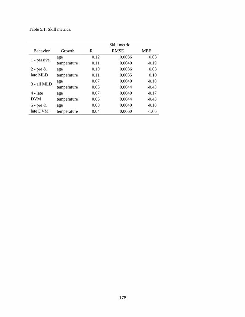
178
Table 5.1. Skill metrics.
Skill metric
Behavior Growth R RMSE MEF
1 - passive age 0.12 0.0036 0.03
temperature 0.11 0.0040 -0.19
2 - pre &
late MLD
age 0.10 0.0036 0.03
temperature 0.11 0.0035 0.10
3 - all MLD age 0.07 0.0040 -0.18
temperature 0.06 0.0044 -0.43
4 - late
DVM
age 0.07 0.0040 -0.17
temperature 0.06 0.0044 -0.43
5 - pre &
late DVM
age 0.08 0.0040 -0.18
temperature 0.04 0.0060 -1.66
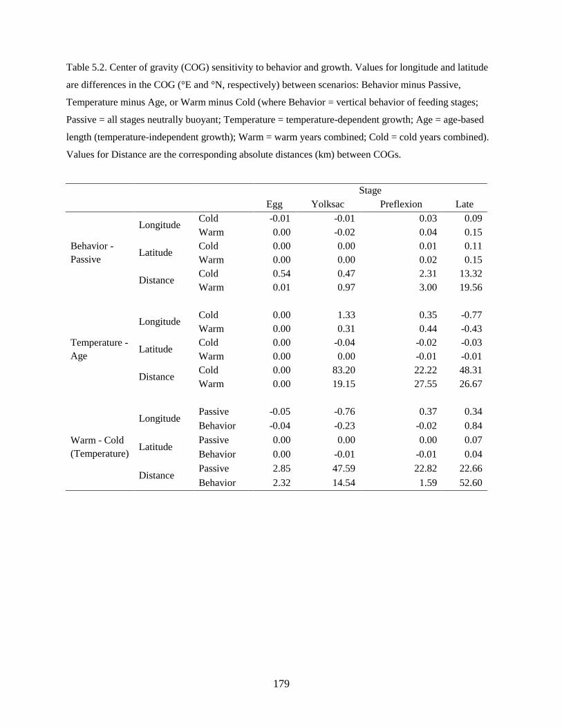
179
Table 5.2. Center of gravity (COG) sensitivity to behavior and growth. Values for longitude and latitude
are differences in the COG (°E and °N, respectively) between scenarios: Behavior minus Passive,
Temperature minus Age, or Warm minus Cold (where Behavior = vertical behavior of feeding stages;
Passive = all stages neutrally buoyant; Temperature = temperature-dependent growth; Age = age-based
length (temperature-independent growth); Warm = warm years combined; Cold = cold years combined).
Values for Distance are the corresponding absolute distances (km) between COGs.
Stage
Egg Yolksac Preflexion Late
Behavior -
Passive
Longitude Cold -0.01 -0.01 0.03 0.09
Warm 0.00 -0.02 0.04 0.15
Latitude Cold 0.00 0.00 0.01 0.11
Warm 0.00 0.00 0.02 0.15
Distance Cold 0.54 0.47 2.31 13.32
Warm 0.01 0.97 3.00 19.56
Temperature -
Age
Longitude Cold 0.00 1.33 0.35 -0.77
Warm 0.00 0.31 0.44 -0.43
Latitude Cold 0.00 -0.04 -0.02 -0.03
Warm 0.00 0.00 -0.01 -0.01
Distance Cold 0.00 83.20 22.22 48.31
Warm 0.00 19.15 27.55 26.67
Warm - Cold
(Temperature)
Longitude Passive -0.05 -0.76 0.37 0.34
Behavior -0.04 -0.23 -0.02 0.84
Latitude Passive 0.00 0.00 0.00 0.07
Behavior 0.00 -0.01 -0.01 0.04
Distance Passive 2.85 47.59 22.82 22.66
Behavior 2.32 14.54 1.59 52.60
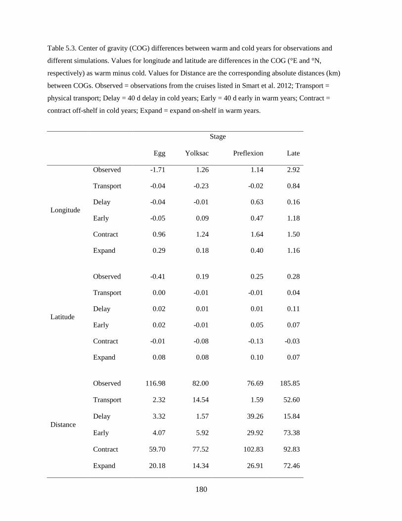
180
Table 5.3. Center of gravity (COG) differences between warm and cold years for observations and
different simulations. Values for longitude and latitude are differences in the COG (°E and °N,
respectively) as warm minus cold. Values for Distance are the corresponding absolute distances (km)
between COGs. Observed = observations from the cruises listed in Smart et al. 2012; Transport =
physical transport; Delay = 40 d delay in cold years; Early = 40 d early in warm years; Contract =
contract off-shelf in cold years; Expand = expand on-shelf in warm years.
Stage
Egg Yolksac Preflexion Late
Longitude
Observed -1.71 1.26 1.14 2.92
Transport -0.04 -0.23 -0.02 0.84
Delay -0.04 -0.01 0.63 0.16
Early -0.05 0.09 0.47 1.18
Contract 0.96 1.24 1.64 1.50
Expand 0.29 0.18 0.40 1.16
Latitude
Observed -0.41 0.19 0.25 0.28
Transport 0.00 -0.01 -0.01 0.04
Delay 0.02 0.01 0.01 0.11
Early 0.02 -0.01 0.05 0.07
Contract -0.01 -0.08 -0.13 -0.03
Expand 0.08 0.08 0.10 0.07
Distance
Observed 116.98 82.00 76.69 185.85
Transport 2.32 14.54 1.59 52.60
Delay 3.32 1.57 39.26 15.84
Early 4.07 5.92 29.92 73.38
Contract 59.70 77.52 102.83 92.83
Expand 20.18 14.34 26.91 72.46

181
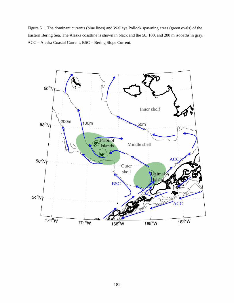
182
Figure 5.1. The dominant currents (blue lines) and Walleye Pollock spawning areas (green ovals) of the
Eastern Bering Sea. The Alaska coastline is shown in black and the 50, 100, and 200 m isobaths in gray.
ACC – Alaska Coastal Current; BSC – Bering Slope Current.
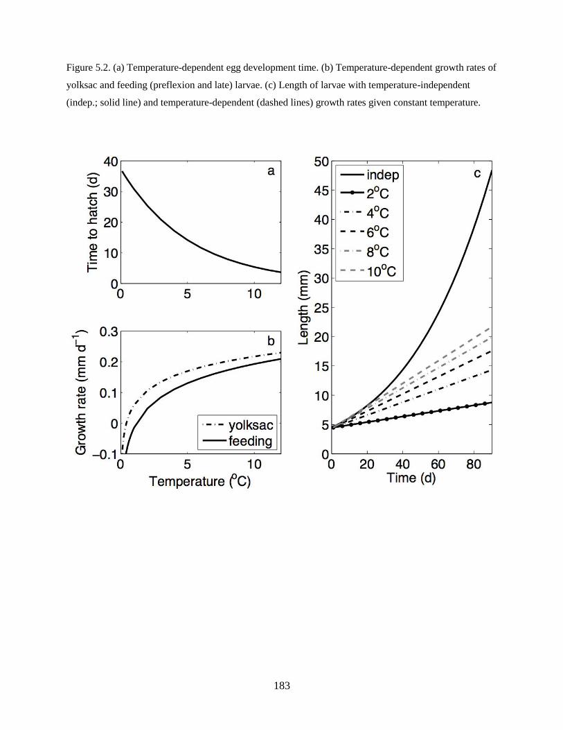
183
Figure 5.2. (a) Temperature-dependent egg development time. (b) Temperature-dependent growth rates of
yolksac and feeding (preflexion and late) larvae. (c) Length of larvae with temperature-independent
(indep.; solid line) and temperature-dependent (dashed lines) growth rates given constant temperature.
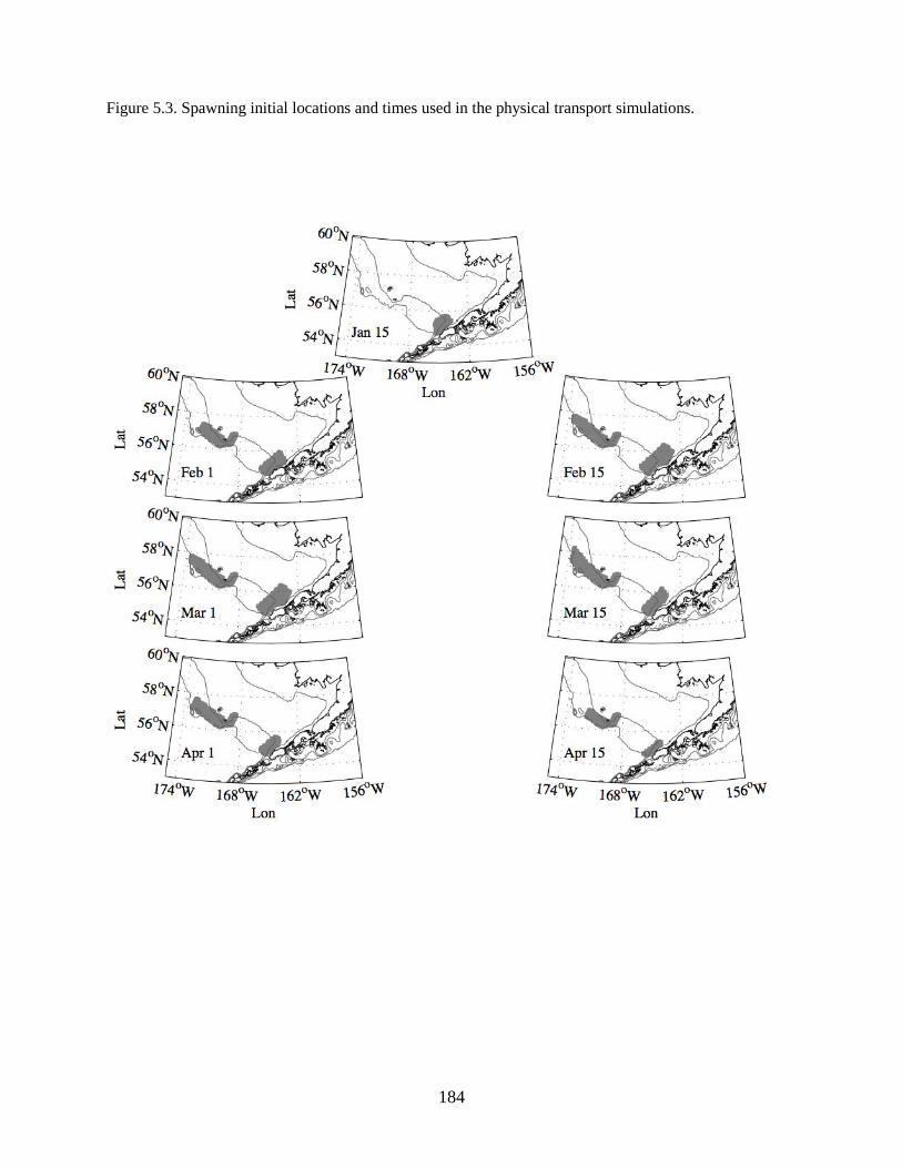
184
Figure 5.3. Spawning initial locations and times used in the physical transport simulations.
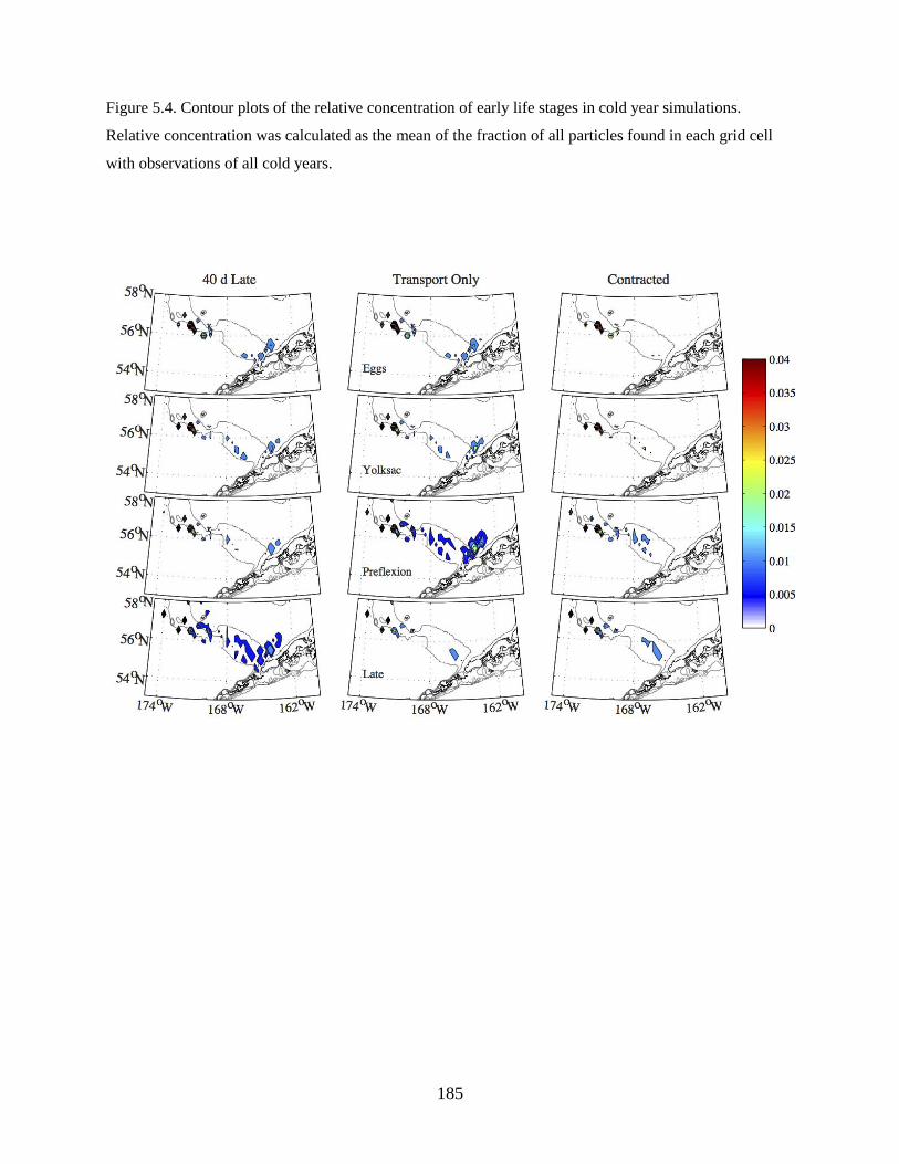
185
Figure 5.4. Contour plots of the relative concentration of early life stages in cold year simulations.
Relative concentration was calculated as the mean of the fraction of all particles found in each grid cell
with observations of all cold years.
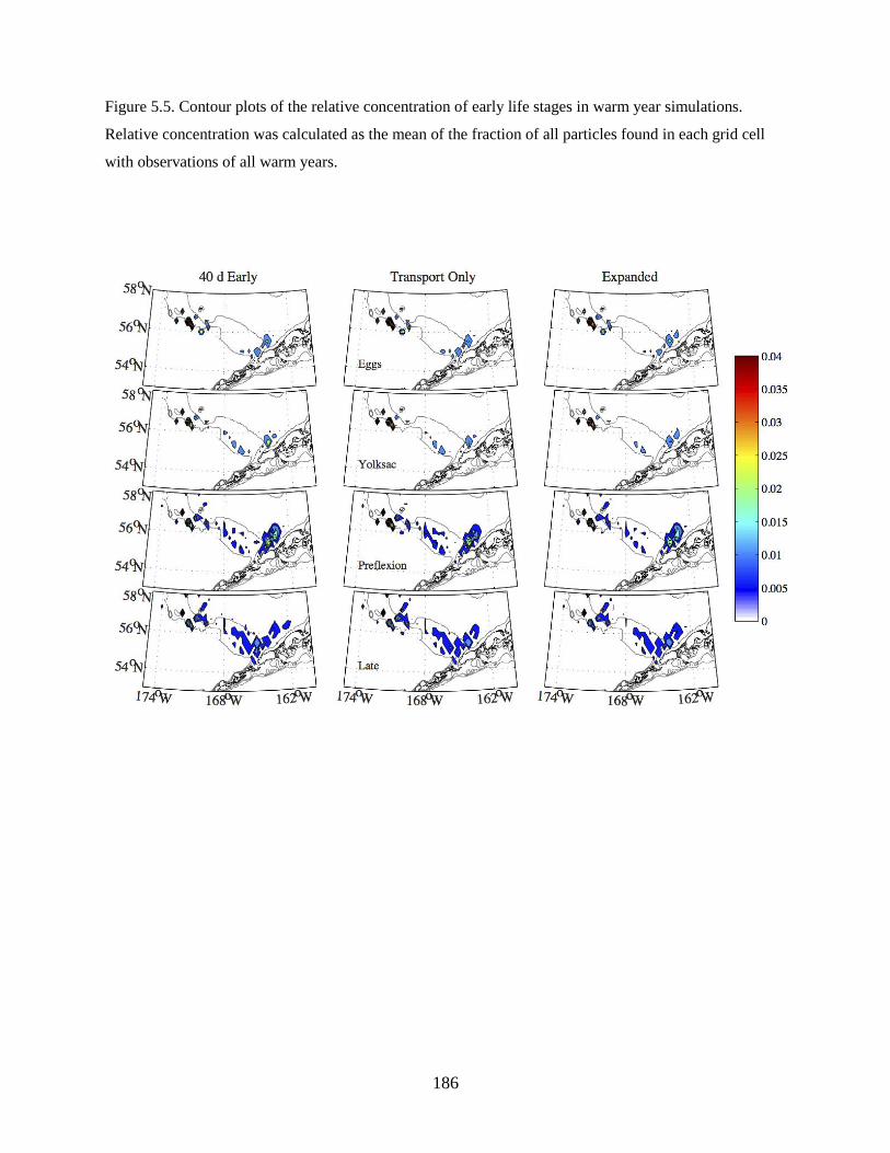
186
Figure 5.5. Contour plots of the relative concentration of early life stages in warm year simulations.
Relative concentration was calculated as the mean of the fraction of all particles found in each grid cell
with observations of all warm years.
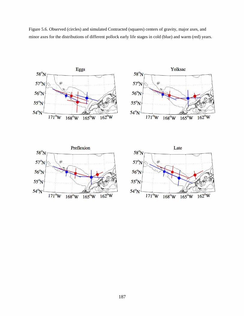
187
Figure 5.6. Observed (circles) and simulated Contracted (squares) centers of gravity, major axes, and
minor axes for the distributions of different pollock early life stages in cold (blue) and warm (red) years.
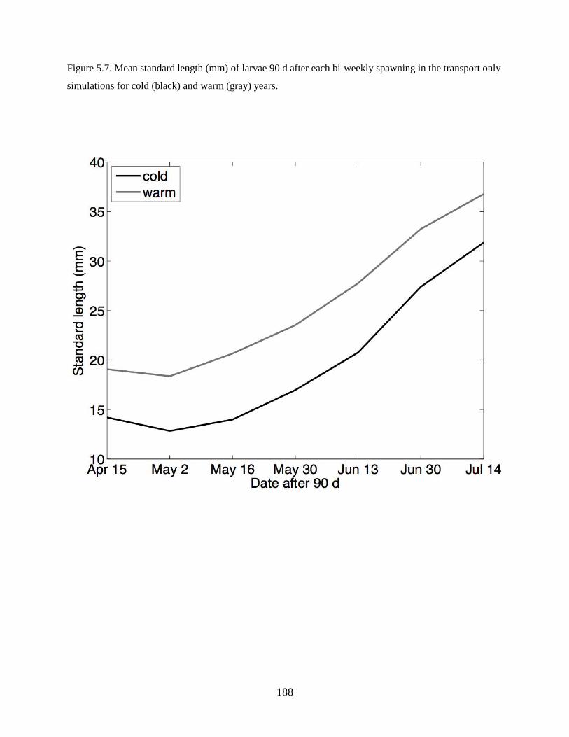
188
Figure 5.7. Mean standard length (mm) of larvae 90 d after each bi-weekly spawning in the transport only
simulations for cold (black) and warm (gray) years.
189
Chapter 6: Ecology and taxonomy of the early life stages of Arrowtooth Flounder (Atheresthes
stomias) and Kamchatka Flounder (A. evermanni) in the eastern Bering Sea
Lisa De Forest1, J.T. Duffy-Anderson
1, R.A. Heintz
2, A.C. Matarese
3, E.C. Siddon
2,
T.I. Smart1, and I.B. Spies
1
1Alaska Fisheries Science Center, National Marine Fisheries Service, National Oceanic and Atmospheric
Administration, Seattle, WA, USA 98115
2Alaska Fisheries Science Center, Auke Bay Laboratories, National Marine Fisheries Service, National
Oceanic and Atmospheric Administration, Juneau, AK, USA 99801
Citation: De Forest, L., Duffy-Anderson, J.T., Heintz, R., Matarese, A.M., Siddon, E., Smart, T. and
Spies, I. In press. Ecology and taxonomy of the early life stages of Arrowtooth (Atheresthes stomias) and
Kamchatka (Atheresthes evermanni) Flounder in the eastern Bering Sea. Deep Sea Research II: Topical
Studies in Oceanography. http://dx.doi.org/10.1016/j.dsr2.2014.05.005
190
Abstract
Arrowtooth Flounder (Atheresthes stomias) and Kamchatka Flounder (A. evermanni) are closely related
flatfish species that co-occur in the eastern Bering Sea. As adults, Arrowtooth Flounder can be
distinguished from Kamchatka Flounder; however, larvae and early juveniles can only be indentified to
the genus level due to morphological similarities. This has precluded studies of ecology for the early life
stages of both species in the eastern Bering Sea. In this study, we developed a genetic technique to
identify the larvae and early juveniles of the two species using mtDNA cytochrome oxidase subunit I
(COI). Genetically identified specimens were then examined to determine a visual identification method
based on pigment patterns and morphology. Specimens 6.0–12.0 mm SL and ≥ 18.0 mm SL can be
identified to the species level, but species identification of individuals 12.1–17.9 mm SL by visual means
alone remains elusive. The distribution of larvae (< 25.0 mm SL) of both Arrowtooth Flounder and
Kamchatka Flounder is similar in the eastern Bering Sea; however, juvenile (≥ 25.0 mm SL) Kamchatka
Flounder occur closer to the shelf break and in deeper water than juvenile Arrowtooth Flounder.
Condition was measured in larvae and juveniles of each species by analyzing lipid content (%) and energy
density (kJ/g dry mass). Kamchatka Flounder larvae on average had higher lipid content than Arrowtooth
Flounder larvae, but were also larger on average than Arrowtooth Flounder larvae in the summer. When
corrected for length, both species had similar lipid content in the larval and juvenile stages.
191
Introduction
Arrowtooth Flounder are large (max. size 86 cm total length), predatory flatfish that occur from
off the coast of central California, north to the Bering Sea, and west to the Kamchatka Peninsula, Russia
(Mecklenburg et al., 2002). Kamchatka Flounder are similar in size, but occur primarily in the western
Bering Sea with lesser occurrence in the eastern Bering Sea and along the Aleutian Islands (Mecklenburg
et al., 2002). In the Bering Sea, Arrowtooth Flounder have been documented to feed primarily on
juvenile and adult Walleye Pollock (Gadus chalcogrammus), euphausiids, and various shrimps (Yang and
Livingston, 1986). They, in turn, are consumed by Alaska Skates (Bathyraja parmifera) and Sleeper
Sharks (Somniosus pacificus) as adults, and by Pacific Cod (Gadus macrocephalus) and Walleye Pollock
as juveniles (Spies et al., 2011). The diet of Kamchatka Flounder is similar and often considered identical
to Arrowtooth Flounder (Yang and Livingston, 1986). Both their predation impact and their role as prey
for other organisms indicate that Arrowtooth Flounder and Kamchatka Flounder are important
constituents of the Bering Sea ecosystem (Aydin et al., 2007). The directed fishing effort for Arrowtooth
Flounder has increased in recent years, as has the retention of adults caught in other commercial fisheries,
possibly in response to an approximate eight-fold increase in adult Arrowtooth Flounder biomass in the
Bering Sea since the early 1980s (Spies et al., 2011). Kamchatka Flounder also experience some fishing
pressure as directed commercial fishing has developed in recent years (Wilderbuer et al., 2011).
Despite their many similarities, these two species can be separated as adults by the number of gill
rakers on the second upper gill arch (one in Kamchatka Flounder, two to three in Arrowtooth Flounder)
and the visibility of the dorsal-most eye from the blind side (top of eye is visible in Arrowtooth Flounder,
no part of eye visible in Kamchatka Flounder) (Yang, 1988). Using electrophoretic examiniation of alleles
at 32 different loci, Ranck et al. (1986) determined that Arrowtooth Flounder and Kamchatka Flounder
were two genetically-distinct species and, based on the distinct distributions of certain alleles, there was
no hybridization between the two species. However, adults of Arrowtooth Flounder and Kamchatka
Flounder collected in scientific and commercial catches were often recorded as either all Arrowtooth
Flounder or the genus Atheresthes (Yang and Livingston, 1986; Spies et al., 2011). In 1991, adult
Arrowtooth Flounder and Kamchatka Flounder individuals began to be separated as distinct species by
the Alaska Fisheries Science Center (AFSC) Groundfish Assessment Program (Zimmerman and Goddard,
1996). As of summer 2011, fishing management regulations dictated that Arrowtooth Flounder and
Kamchatka Flounder must be separated and recorded as distinct species in commercial fishing hauls due
to the emergence of a directed fishery for adult Kanchatka Flounder (Wilderbuer et al., 2011).
While adults of both species have been well described, the early life stages in the eastern Bering
Sea have not been. High recruitment success may be the cause of the increase in population size of
Arrowtooth Flounder in recent years (Spies et al., 2011). Understanding the early life stages is important
192
to understanding recruitment and the first step to understanding recruitment in Arrowtooth Flounder is to
identify and separate the early life stages from Kamchatka Flounder. Our current study had the following
objectives: 1) use genetic methods to identify to the species level larval and early juvenile Atheresthes
collected in the eastern Bering Sea, 2) use the genetically identified individuals to develop a visual
identification method that allows identification of historical and future samples, 3) describe the
distribution and abundance of the early life stages of both Arrowtooth Flounder and Kamchatka Flounder,
and 4) examine condition as indicated by length adjusted dry mass, lipid content (%), and energy density
of larvae and juveniles to determine differences in nutritional quality between species.
Methods
Specimen collection
All specimens in this study were either directly collected at sea or were sorted from previously
collected preserved samples collected on previous AFSC ichthyoplankton surveys. The specimens
collected at sea were obtained on spring and summer cruises from 2006 to 2010 by scientists on AFSC,
Bering Ecosystem Study (BEST), and Bering Sea Integrated Ecosystem Research Program (BSIERP)
cruises (Table 6.1). Specimens were collected opportunistically, resulting in varied collection and
preservation methods during the study. Methods of collection included using bongo nets (60-cm; 500-µm
mesh), Multiple Opening/Closing Net and Environmental Sensing System (MOCNESS; 1-m2 with 500-
µm mesh; Wiebe et al., 1976), and surface and midwater trawls. Specimens removed from the bongo net
were either placed directly into 100% non-denatured ethanol or into 5% formalin after an eyeball was
removed. Sampling from the MOCNESS involved removing specimens only from the drogue net, which
was open for the duration of the tow; all specimens were immediately frozen at -80º C. The surface and
midwater rope trawls sampled above and below the pycnocline; all specimens collected were immediately
frozen at -80º C. Specimens sorted from previously collected preserved samples were chosen from cruises
occurring from 1994 to 2010 (Table 6.1). The samples were collected on previous AFSC ichthyoplankton
surveys using 60-cm bongo nets, MOCNESS tows, Methot trawls (Methot, 1986), Tucker trawls (1-m2
with 500-µm mesh; Tucker, 1951), and a modified bottom trawl (which samples the midwater). Sampling
protocol during the cruises, along with sample handling and sorting, follows Matarese et al. (2003). All
specimens used in this study were classified as either larvae (3.0–24.9 mm SL) or juveniles (≥ 25.0 mm
SL) (Matarese et al., 1989).
Genetic identification
193
Species determination was based on a restriction enzyme digest that cuts DNA at a specific
nucleotide sequence that is present in Arrowtooth Flounder but not Kamchatka Flounder. The test was
based on an initial sequencing of three adult specimens from each species, followed by testing on 20 adult
specimens of which the species identification was known. Fin tissue was used for DNA extraction in all
adults and was performed using Qiagen DNA extraction kits (Qiagen, Inc. Valencia, CA). For larval and
early juveniles, a single eyeball (from either side of head) removed from either fresh, frozen, or 100%
non-denatured ethanol preserved specimens was used for DNA extraction. The rest of the specimen body
was placed back in its original preservative or, if frozen, photographed for future visual identification
work.
Larval DNA was extracted from a single eyeball using a standard Chelex DNA extraction
protocol. The eyeball was submerged in 150 µl of 10% (w/v) Chelex ® 100 resin (BIO-RAD Laboratories,
Hercules, CA), heated to 60° C for 20 min followed by 103° C for 25 min. A 750 bp segment of
cytochrome oxidase subunit I (COI) was amplified using the following primers: COI_RajaF (5’-
CCGCTTAACTCTCAGCCATC-3’) and COI_RajaR (5’-TCAGGGTGACCAAAGAATCA-3’; Spies et
ng DNA (1 µl taken from the Chelex supernatant), 10 mM Tris-HCl (pH 8.3), 50 mM KCl, 3.0 mM
MgCl2, 1.5 mM dNTPs, 0.5 pM of each primer, and 0.5 U Bioline Taq polymerase (Bioline USA, Inc.,
Boston, MA). PCR amplification using Chelex extractions can fail if the supernatant contains impurities
such as proteins. Therefore, failed samples were repeated with a 1:10 or 1:100 dilution of the DNA, which
typically resulted in success. The thermal cycling protocol consisted of 94° C for 2 min, followed by 40
cycles of 94° C (30 seconds), 57°C (30 sec), and 72° C (30 sec). DNA sequencing of amplified DNA
from adult specimens was performed using COI_Raja primers at the University of Washington High
Throughput Genomics Center (www.htseq.org).
Following PCR, DNA was digested using Bmt1 (New England Biolabs, Ipswich, MA) according
to manufacturer’s instructions, in a total volume of 10:l with 2:l PCR product and 4 U of Bmt1 at 37° C
for 1 h. Identification was based on either the presence of a single 750 bp fragment (Kamchatka Flounder)
or two fragments consisting of 450 and 300 bp (Arrowtooth Flounder).
This protocol was performed in a laboratory or at sea using an Agilent 2100 Bioanalyzer with a
DNA 1000 kit (Agilent Technologies, Santa Clara, CA) and a BIO-RAD DNA Engine Thermalcycler.
Visual identification
194
Specimens identified using genetic methods were examined to develop a visual identification
method based on morphological and pigmentation characters. Specimens were examined both with and
without knowledge of their genetic identification to determine species-specific characters. Each specimen
was critically evaluated with regards to morphology and pigment (such as the number of melanophores in
a patch or the general shape and pattern of melanophore patches). Only specimens preserved in the same
preservation medium were directly compared to one another. This was to minimize the identification of
preservation artifacts as distinguishing species characters.
Morphometric measurements were taken from Arrowtooth Flounder and Kamchatka Flounder
larvae chosen from a single cruise. Only specimens initially preserved in formalin were used for
morphometric measurements because the other preservation methods (100% ethanol and immediate
freezing) shrink tissues and distort morphology. The following measurements were taken: standard length
(SL), preanal length (tip of snout to anus), head length, snout length, eye diameter, and body depth
(vertical measurement taken at pectoral fin; BD). The measurements were taken using a calibrated digital
image analysis system consisting of a video camera attached to a stereo microscope and a computer with
image analysis software. All measurements were recorded to the nearest 0.1 mm. A two sample t-test was
used to identify statistically significant differences (p < 0.05) between each morphological measurement
for the two species. Developmental stage terminology follows Kendall et al. (1984).
Distribution
Selected larval Atheresthes collected on previous AFSC cruises conducted from 1994 to 2010
(Table 6.1) were identified to the species level using pigmentation and morphological characters
identified with the visual identification method. The locations of all specimens identified to species were
mapped and a mean distribution based on abundance was calculated for each species using ArcGIS
software.
Measures of Condition
Biological sampling
Larval and juvenile Atheresthes were collected from five research surveys conducted in the summer and
early fall from 2008 to 2010 (Table 6.1). All specimens were measured to the nearest 0.01 mm SL.
Specimens < 30.0 mm SL were identified to species using the genetic methods previously described,
while specimens > 30.0 mm SL were identified morphologically using the number of gill rakers on the
upper arch of the second gill raker. All specimens had an eyeball removed, even if identified visually.
Stomach contents were removed prior to chemical analysis.
195
Dry mass
Larvae were individually dried at 60ºC in a drying oven until their weight was stabilized.
Juveniles were dried at 135ºC using a LECO Thermogravimetric Analyzer (TGA) 601 or 701, which
provided percent moisture values used to convert wet mass to dry mass equivalents.
Estimation of lipid content (%)
For larvae, a sulfo-phospho-vanillin (SPV) colorimetric analysis (Van Handel, 1985) was
performed to determine lipid content (%). Dried material was sonicated in 2:1 (by volume)
chloroform:methanol solvent in glass centrifuge tubes for 60 min. Washes of 0.88% KCL and 1:1 (by
volume) methanol:water were performed on the extracts as in the modified Folch extraction method
(Vollenweider et al., 2011). Resulting chloroform extracts were evaporated in a LabConco RapidVap for
30 min at 40 ºC and 250 mbar until reduced to approximately 1 ml in volume. Extracts were evaporated to
dryness in 12 mm test tubes on a heating block at 75 ºC and then allowed to cool. Concentrated sulfuric
acid was added to the tubes prior to incubation at 100 ºC for 10 min with subsequent cooling. The SPV
reagent (1.2 mg/ml vanillin in 80% phosphoric acid) was added to each tube and allowed to develop for
10 min. Absorption was measured on an Agilent 8453 Spectrophotometer at 490 nm and extrapolated
from species-specific calibration curves determined prior to analysis. For juveniles, lipid extraction was
performed on dried material using a previously described method (Vollenweider et al., 2011) derived
from the Folch extraction procedure.
Energy density
Energy density (kJ/g dry mass) was estimated using bomb calorimetry. Homogenized dry tissue
was pressed into a pellet form and a Parr Instrument 6725 Semimicro Calorimeter with 6772 Precision
Thermometer and 1109A Oxygen Bomb was used to measure the energy released from combustion of the
sample pellets. The minimum pellet weight was set at 0.025 g of dry material based on the limits of
instrument detection; individual larvae were composited within stations as needed to attain sufficient dry
mass.
Statistical analysis
A general linear model was used to identify differences in the nutritional state of Arrowtooth
Flounder and Kamchatka Flounder. Lengths were compared by a nested analysis of variance (ANOVA)
to account for differences in the numbers of fish collected. Species was the main factor with life stage
nested in species and year nested in life stage. Post-hoc comparisons of species were conducted among
the life stages using Bonferonni’s adjusted t value. Analysis of covariance (ANCOVA) was employed to
196
compare dry mass and lipid content between species. This approach permitted comparisons when length
distributions differed between species and the responses covaried with length. The ANCOVA used
species, year, and their interaction as main factors and length as covariate. Analyses were conducted
separately for larvae and juveniles because the response variables were heteroscedastic when pooled
across life stages. Variables were transformed prior to analysis using logarithms (base 10), and the
assumption that both species had equivalent slopes was tested. Student’s t was used to compare energy
densities of larvae and juveniles.
Results
Genetics
Using mtDNA COI restriction analysis proved successful in identifying Atheresthes larvae and
early juveniles to species in the laboratory (n = 337) and at sea (n = 78). Of the 415 total specimens, 165
were identified as Arrowtooth Flounder, 194 as Kamchatka Flounder, and 56 failed to amplify properly
resulting in an unknown identity. Size of specimens examined was 6.0–38.0 mm SL, with the majority of
specimens 6.0–11.5 mm SL.
Visual identification
Visual examination of genetically-identified specimens was successful in determining key
pigmentation differences between Arrowtooth Flounder and Kamchatka Flounder larvae of 6.0–12.0 mm
SL and ≥ 18.0 mm SL. These key pigmentation differences are size specific but not stage specific.
Specimens 12.1–17.9 mm SL remain indistinguishable at this time because of the small sample size and a
high degree of variation in pigmentation patterns.
Recently hatched Kanchatka Flounder larvae (6.0–7.4 mm SL) can be distinguished from
Arrowtooth Flounder of the same size by the presence of pigment dorsal to the gut at the anus and an
anterior dorsal pigment patch located halfway between the anus and the caudal fin (Figure 6.1a).
Arrowtooth Flounder begin to develop the same pigment patterns at about 7.5 mm SL, resulting in these
characteristics no longer being able to be used.
Larvae of 7.5–12.0 mm SL can be identified by two characters. Kamchatka Flounder larvae of
7.5–10.5 mm have pigment on the crown of the head, beginning as a few melanophores and developing to
numerous melanophores that cover the entire crown of the head by approximately 9.0 mm SL (Figure
6.1a). In general, Arrowtooth Flounder larvae do not begin to develop head pigment prior to 10.5 mm SL,
however, a few individuals do develop one or two two small melanophores on the crown of the head
beginning at approximately 8.5 mm SL (Figure 6.1b). Thus, specimens 8.5–10.5 mm SL with only 1–3
197
melanophores on the head cannot be identified to species. In addition to crown pigment, the second
character by which Kamchatka Flounder larvae 7.5–12.0 mm SL can be identified is the pigment dorsal to
the gut that starts at mid gut and extends to the anus (Figure 6.1a). Arrowtooth Flounder larvae also have
pigment dorsal to the gut, but it starts at ¾ gut length and extends to the anus. The combination of these
two characters allows larvae 7.5–12.0 mm SL to be identified to species.
Few genetically identified specimens were larger than 12.0 mm SL. Identification methods for
larger specimens began with the use of adult characters to identify specimens > 25.0 mm SL. These
identified specimens were then used as a guide to begin identifying smaller specimens. The adult
characters used to determine the larger specimens were the number of gill rakers on the second upper gill
arch: Kamchatka Flounder have one gill raker, Arrowtooth Flounder have two or three. While these
structures are not fully formed in specimens of 25.0–27.0 mm SL, fleshy protrusions that are the
precursors to the gill rakers are evident. After numerous specimens were separated based on gill raker
counts, a pattern in the dorsal pigment bands was seen to be different between the two species. The
anterior dorsal patch on Kamchatka Flounder is generally longer (> 5 melanophores long) and the
individual melanophores in the patch are close together, often touching and at times coalescing.
Additionally, Kamchatka Flounder develop melanophores between the anterior and posterior bands,
which eventually connect the two bands at a smaller size than Arrowtooth Flounder (beginning as early as
approximately 13.0 mm SL, but generally by 18.0 mm SL) (Figure 6.1a). In contrast, Arrowtooth
Flounder tend to have a short (< 5 melanophores long) anterior dorsal band with melanophores that are
widely spaced apart. Melanophores do not develop between the anterior and posterior dorsal bands until
approximately 25.0 mm SL (Figure 6.1b). The few large larvae and early juveniles used in the genetic
technique confirmed the validity of these visual differences.
Morphological measurements were taken on 20 Arrowtooth Flounder larvae and 19 Kamchatka
Flounder larvae. Specimens ranged in length from 6.3 to 12.6 mm SL. Head length and eye diameter were
not statistically different between the two species, but body depth and preanal length were. Larvae of
Kanchatka Flounder have a stouter body (BD = 12.0 ± 1.1% SL) than Arrowtooth Flounder larvae (BD =
9.8 ± 1.4% SL; p < 0.05). In addition to a stouter body, Kamchatka Flounder larvae also have a slightly
longer preanal length than Arrowtooth Flounder larvae (36.3 ± 1.8% SL vs. 35.1 ± 1.8% SL; p < 0.05).
Distribution
Examining formalin-preserved specimens from previous AFSC cruises, a total of 1,928 larvae
and juveniles were identified to species using pigmentation and morphological characters identified
above, with 364 individuals identified to genus because of ambiguous characters or damage. A total of
198
1,315 Arrowtooth Flounder larvae and 480 Kamchatka Flounder larvae were identified; 125 Arrowtooth
Flounder juveniles and eight Kamchatka Flounder juveniles were identified.
The majority of larval Arrowtooth Flounder and Kamchatka Flounder were collected along the
shelf break in the southeastern Bering Sea between Unimak and Umnak Pass (Figure 6.2). There were
also individuals collected farther north in Pribilof Canyon along the shelf break near deep water. The
calculated mean distribution for both species is similar (Figure 6.2).
Juveniles of both species were collected primarily north of where the majority of the larvae were
collected. The calculated mean distribution of the two species showed that Arrowtooth Flounder juveniles
appear to be located farther east and over shallower waters than Kamchatka Flounder juveniles, which
have a mean distribution close to Pribilof Canyon and deeper water (Figure 6.2). However, fewer
Kamchatka Flounder juveniles were collected and identified (n = 8) than Arrowtooth Flounder juveniles
(n = 125), so caution should be used when interpreting this result.
Measures of condition
Biological sampling
Length analysis was restricted to larvae collected in 2009 and 2010 and juveniles collected in
2010. These were stages and years in which sufficient numbers of specimens were collected. No
significant difference was found in the lengths of larvae or juveniles sampled in 2009 and 2010 (F2.154 >
0.77, p = 0.466), and larvae were significantly smaller than juveniles (F2.154 > 1000, p < 0.001). Pairwise
comparisons of larvae and juveniles between the two species averaged across years indicated that
Kamchatka Flounder larvae averaged approximately 25% longer than Arrowtooth Flounder larvae (t =
4.6, p < 0.001), but no difference was detected among juveniles (t = 0.31, p = 0.991) (Table 6.2).
Differences between the two sets of larvae therefore accounted for the overall difference detected between
species (F1.154 = 6.71, p = 0.010).
Dry mass
The dry weights of larvae did not depend on year nor was there an interaction between year and
species (F1.96 < 0.15, p > 0.700). However, larval Arrowtooth Flounder of a fixed length were
approximately 25% lighter than similarly sized Kamchtaka Flounder (F1.96 = 4.16, p = 0.044; Figure 6.3a).
No difference in dry mass was detected among juvenile specimens in 2010 (F1.53 = 1.68, p = 0.20; Figure
6.3b). It was not possible to test for year effect due to an inadequate number of samples in 2008 and 2009.
199
Lipid content
In 2009 and 2010 the average lipid content of arrowtooth larvae was 7.5 ± 0.3% (n = 39) of dry
mass compared with 10.8 ± 0.7% for Kamchatka Flounder larvae (n = 11; Figure 6.4a). While the lipid
content of Kamchatka Flounder larvae averaged approximately 30% more than that of Arrowtooth
Flounder larvae, this difference was not significant after controlling for the differences in average length
(F1.45 = 3.15, p = 0.083). Additionally, there was not an effect of year or interaction between year and
species on larval lipid content (F1.45 < 2.37, p > 0.130). In 2010, there was no difference between
juveniles (F1.25 = 0.03, p = 0.857). Arrowtooth Flounder juveniles averaged 10.2 ± 0.5% lipid (n = 21) in
2010 compared with 10.7 ± 0.7% (n = 7) for Kamchatka Flounder juveniles.
Energy density
Energy density in juveniles was only measured in 2010 and in larvae only in 2009. Only a few
larvae could be measured because samples required compositing. There was no statistically significant
difference between the energy densities of the two species. Only six measurements of larval energy
density were taken and the difference between species was not statistically significant (t = 1.06, p =
0.366) (Figure 6.4b). Arrowtooth Flounder larvae averaged 19.2 ± 0.8 kJ/g dry mass; Kamchatka
Flounder larvae averaged 19.8 ± 0.7 kJ/g dry mass. Energy densities between juveniles of the two species
were nearly identical (t = 1.19, p = 0.244), averaging 20.5 ± 0.2 kJ/g dry mass for Arrowtooth Flounder (n
= 16) and 20.8 ± 0.2 kJ/g dry mass for Kamchatka Flounder (n = 12).
Discussion
With the increasing population size of Arrowtooth Flounder and interest for increased directed
fishing effort for both Arrowtooth Flounder and Kamchtaka Flounder, there is a need to fully identify and
study both species in all life stages for management and ecological purposes. Adults of Arrowtooth
Flounder have been studied with regard to their distribution (Zimmerman and Goddard, 1996), predation
effects on Walleye Pollock (Ianelli et al., 2009), and their role as prey for other organisms (Livingston
and Jurado-Molina, 2000). The early life stages in the Gulf of Alaska have been described by Blood et al.
(2007); however, efforts to conclusively identify larvae and juveniles in the Bering Sea have been
confounded by the overwhelming physical similarities between Arrowtooth and Kamchatka Flounder.
Genetics
Genetic methods have proven to be useful tools in identifying unknown specimens to the species
or family level using the mtDNA gene COI (Hebert et al., 2002; Dawnay et al., 2007; Rocha et al., 2007).
In Alaskan waters, Spies et al. (2006) also successfully used mtDNA COI to identify 15 different skate
200
species. In this current study we have demonstrated that this genetic technique is valid for identifying
specimens of Atheresthes to the species level. In addition, the technique developed in this study proved
effective for use both in the laboratory and at sea aboard a research vessel. In particular, this ability to
conclusively identify specimens to the species level while at sea is quite useful as it can enable a timely
adjustment to sampling location or procedure in order to maximize collection of the target species.
Morphology
In the marine environment closely related species are often indistinguishable as larvae due to
overlap in pigmentation and morphological characters. Prior to this study, all larval and early juvenile
Atheresthes collected in the Bering Sea were identified only to the genus level. Despite numerous
physical similarities, unique pigmentation and morphological differences were noted between the two
Atheresthes species in the size ranges of 6.0–12.0 mm SL and ≥ 18.0 mm SL. In general, it appears that
Kamchatka Flounder acquire certain pigmentation characters at smaller sizes than Arrowtooth Flounder,
thus the distinguishing characters noted in this paper can only be used for the specific size ranges to
which they correspond. Specimens of 12.1–17.9 mm SL are indistinguishable at this time due because of
a high degree of variability in pigment amongst individuals and a low number of genetically identified
specimens in this size range. In addition to pigment, larvae are stouter than Arrowtooth Flounder larvae
(BD 12.0% SL vs. 9.8% SL) and have a slightly longer snout to anus length (36.3% SL vs. 35.1% SL).
These are modest morphological differences and can be difficult to determine but can be helpful when
used in conjunction with pigmentation characters to support species identification.
Using the pigment characteristics described in this study, two specimens illustrated by Blood et
al. (2007; Figure 6.13) should be re-examined as both specimens were collected in the Bering Sea. The
13.4 mm SL specimen is most likely Kamchatka Flounder, not Arrowtooth Flounder, based on the large
amount of pigment present on the head and the pigment present on the dorsal midline between the two
dorsal bands. While Arrowtooth Flounder develop pigment on the crown of the head, the amount of
pigment present at this size is more indicative of Kamchatka Flounder. In addition, the presence of
pigment on the dorsal midline between the two dorsal bands at this size can only be Kamchatka Flounder
as arrowtooth do not develop this pigment until approximately 25.0 mm SL. The 10.0 mm SL specimen
(Blood et al., 2007; Figure 6.12) may also be a Kamchatka Flounder due to the large amount of pigment
located on the crown of the head and within the two dorsal patches. However, complete identification is
difficult from the illustrations alone; a close visual examination of the original specimens is needed.
Distribution
201
The larval distributions of Arrowtooth Flounder and Kamchatka Flounder in the eastern Bering
Sea are similar. Most of the larvae collected were located in the southern part of the eastern Bering Sea in
water > 200 m along the shelf break (Figure 6.2a, b). This may indicate that in the eastern Bering Sea
both arrowtooth and Kamchatka Flounder adults spawn in deep water, similar to that described for
Arrowtooth Flounder in the Gulf of Alaska by Blood et al. (2007). The distribution of juveniles collected
does appear to be different between the two species, but this result is tenuous due to the low number of
juvenile Kamchatka Flounder collected (n = 8). However, this result may indicate that juvenile
Kamchatka Flounder are migrating to their adult habitat. In general, the majority of adult Kamchatka
Flounder are collected in deeper waters and farther to the west than adult Arrowtooth Flounder, which
often occur in shallower waters to the east (Zimmerman and Goddard 1996; Wilderbuer et al., 2011). It is
possible that the low number of juvenile Kamchatka Flounder collected is due to limited sampling in
deeper waters to the west of the shelf break.
Condition
Differences in the condition between Arrowtooth Flounder and Kamchatka Flounder larvae
collected in the summer may relate to differences in timing of development. For years in which sufficient
numbers of larvae were collected for analysis, Kamchatka Flounder larvae were significantly larger than
Arrowtooth Flounder larvae in the summer. Comparison of the lengths of larvae sampled in the summer
indicates that the bulk of Arrowtooth Flounder larvae were in the preflexion or flexion stages (Blood et
al., 2007). Assuming stage designation is similar for Kamchatka Flounder, the majority of Kamchatka
Flounder sampled in the summer were in the flexion and postflexion stages. The difference in
developmental stage could account for the differences in the length adjusted dry mass of the two species
and the trend towards increased lipid content in larval Kamchatka Flounder. Energy allocation strategies
can differ among developmental stages during the early life stages. This study suggests that postflexion
larvae of Atheresthes may invest more energy accreting tissue mass than earlier stages. Comparison of the
lengths of juveniles sampled indicates that the majority of the fish sampled from both species were in the
transformation stage (Blood et al., 2007). Hence there were no differences in condition between juveniles
of either species.
The results presented here are the first estimates of lipid and energy density in larval and juvenile
Arrowtooth Flounder and Kamchatka Flounder. Lipid content values of juveniles in this study are similar
to those reported for Atlantic Halibut (Hippoglossus hippoglossus) fed a diet that promoted growth and
survival (Hamre et al., 2002). Energy densities of larvae were similar to those of juveniles and suggests
no change in energy allocation strategy between these two stages. This is in contrast to Walleye Pollock
which undergo significant changes in both lipid content and energy density between lengths of 20 and 60
mm (Siddon et al., 2012), which is when Walleye Pollock undergo and complete transformation to the
202
juvenile stage (Brown et al., 2001). The only evidence of a shift in lipid content among both species of
Atheresthes sampled here is associated with ontogeny in the larval stages.
Conclusion
This study has provided a method to genetically identify larval and early juvenile Arrowtooth
Flounder and Kamchatka Flounder both in the field and in the laboratory, and has provided morphological
and pigmentation characters to visually identify these two species at small (6.0–12.0 mm SL) and large
sizes (≥ 18.0 mm SL). Future sampling effort during June–August when Arrowtooth Flounder and
Kanchatka Flounder larvae 12.1–17.9 mm SL are in the water column could aid in completing the visual
identification of these two species. Once all Arrowtooth Flounder and Kamchatka Flounder between 6.0
mm SL to the juvenile stage can be identified, all historical samples of Atheresthes collected in 1991–
2010 (19 years) by the AFSC from the eastern Bering Sea can be re-identified to the species level. This
collection contains approximately 5,065 individuals that, when identified to the species level, will greatly
increase our knowledge of distribution and abundance for these two species. Additionally, increased
sampling effort in the deeper water off the shelf break during summer and fall would help define the
distribution of the larger sizes of these two species and determine if there is a difference in timing of
development for larvae in the summer.
Acknowledgements
The authors would like to thank all the scientists that collected Atheresthes spp., larvae over the years and
the officers and crews of the following ships: NOAA ship Miller Freeman, NOAA ship Oscar Dyson,
R/V Thomas G. Thompson, USCGC Healy, and the R/V Knorr. We would also like to thank Dan Cooper
for his help with genetic identification of specimens while on the May 2010 cruise and for reviewing a
draft of this manuscript, Melanie Paquin for her help with genetic identification and sequencing in the
laboratory, Ashlee Overdick for her illustrations of both species, and Debbie Blood for also reviewing a
draft of this manuscript. This is BEST-BSIERP Bering Sea Project publication number XX. This research
is contribution EcoFOCI-XXX to NOAA’s Fisheries-Oceanography Coordinated Investigations. The
findings and conclusions in this manuscript are those of the authors, and do not necessarily represent the
views of the National Marine Fisheries Service.
Literature Cited
Aydin, K., Gaichas, S., Ortiz, I., Kinzey, D., and Friday, N. 2007. A comparison of the Bering Sea, Gulf
of Alaska, and Aleutian Islands large marine ecosystems through food web modeling. U.S. Dept.
Commer., NOAA Tech. Memo. NMFS-AFSC-178, 298 p.
203
Blood, D.M, Matarese, A.C., and Busby, M.S. 2007. Spawning, egg development, and early life history
dynamics of Arrowtooth Flounder (Atheresthes stomias) in the Gulf of Alaska. NOAA
Professional Paper NMFS 7, 28 p.
Brown, A.L., Busby, M.S., and Mier, K.L. 2001. Walleye Pollock Theragra chalcogramma during
transformation from the larval to the juvenile stage: otolith and osteological development. Mar.
Biol. 139: 845-851
Dawnay, N., Ogden, R., McEwing, R., Carvalho, G.R., and Thrope, R.S. 2007. Validation of the
barcoding gene COI for use in forensic genetic species identification. Forensic Sci. Int. 173:1-6.
Hebert, P.D.N., Cywinska, A., Ball, S.L., and deWaard, J.R. 2002. Biological identifications through
DNA barcodes. Proc. R. Soc. Lond. B. 270: 313-321.
Hamre, K., Opstad, I., Espe, M., Solbakken, J., Hemre, G.I., and Pittman, K. 2002. Nutrient composition
and metamorphosis success of Atlantic halibut (Hippoglossus hippoglossus, L.) larvae fed natural
zooplankton or Artemia. Aquac. Nutr. 8: 139-148
Ianelli, J.N., Barbeaux, S., Honkalehto, T., Kotwicki, S., Aydin, K., and Williamson, N. 2009.
Assessment of the Walleye Pollock stock in the Eastern Bering Sea. In: Stock assessment and
fishery evaluation report for the groundfish resources of the Bering Sea/Aleutian Islands regions.
North Pacific Fishery Management Council, 605 W. 4th Ave., Suite 306, Anchorage, AK 99501.
Kendall, A.W., Jr., Ahlstrom, E.H., and Moser, H.G. 1984. Early life history stages and their characters.
In: Ontogeny and systematic of fishes. (H.G. Moser, W.J. Richards, D.M. Cohen, M.P. Fahay,
A.W. Kendall Jr., and S.L. Richardson, eds). P. 11-22. Spec. Publ. 1 Am. Soc. Ichthyol. Herpetol.
Allen Press, Lawrence, KS.
Livingston, P.A., and Jurado-Molina, J. 2000. A multispecies virtual population analysis of the eastern
Bering Sea. ICES J. Mar. Sci. 57: 294-299.
Matarese, A.C., Blood, D.M., Picquelle, S.J., and Benson, J.L. 2003. Atlas of abundance and distribution
patterns of ichthyoplankton from the northeast Pacific Ocean and Bering Sea ecosystems based
on research conducted by the Alaska Fisheries Science Center (1972-1996). NOAA Prof. Paper
NMFS 1, 281 p.
Matarese, A.C., Kendall, A.W. Jr., Blood, D.M., and Vinter, B.M. 1989. Laboratory guide to early life
history stages of northeast Pacific fishes. U.S Dep. Commer. NOAA Tech. Rep. NMFS 80, 652 p.
204
Mecklenburg, C.W., Mecklenburg, T.A., and Thorsteinson, L.K. 2002. Fishes of Alaska. American
Fisheries Society, Bethesda, MD, 1116 p.
Methot, R.D. 1986. Frame trawl for sampling juvenile fish. Calif. Coop. Oceanic Fish. Invest. Rep. 27:
267-278
Ranck, C.L., Utter, F.M., Milner, G. B., and Smith, G. B. 1986. Genetic confirmation of specific
distinction of Arrowtooth Flounder, Atheresthes stomias, and Kamchatka flounder, A. evermanni.
Fish. Bull. 84: 222-226.
Rocha, L.A., Craig, M.T., and Bowen, B.W. 2007. Phylogeny and the conservation of coral reef fishes.
Coral Reefs. 26: 501-512.
Siddon, E.C., Heintz, R.A., and Mueter, F.J. 2013. Conceptual model of energy allocation in Walleye
Pollock (Theragra chalcogramma) from age-0 to age-1 in the southeastern Bering Sea. Deep-Sea
Res. II. 94: 140-149.
Spies, I.B., Gaichas, S., Stevenson, D.E., Orr, J.W., and Canino, M.F. 2006. DNA-based identification of
Alaska skates (Amblyraja, Bathyraja and Raja: Rajidae) using cytochrome c oxidase subunit I
(coI) variation. J. Fish. Biol. 69(B): 283-292.
Spies, I.B., Wilderbuer, T.K., Nichol, D.G., and Aydin, K. 2011. Assessment of the Arrowtooth Flounder
stock in the Bering Sea/Aleutian Islands. North Pacific Management Council, p. 727-744.
Tucker. G.H. 1951. Relation of fishes and other organisms to the scattering of underwater sound. J. Mar.
Res. 10(2): 215–238.
Van Handel, E. 1985. Rapid determination of total lipids in mosquitoes. J. Am. Mosq. Control Assoc. 1
(3): 302-304.
Vollenweider, J.J., Heintz, R., Schaufler, L., and Bradshaw, R. 2011. Seasonal cycles in whole-body
proximate composition and energy content of forage fish vary with water depth. Mar. Biol. 158,
413-27.
Wiebe, P.H., Burt, K.H., Boyd, S.H., and Morton, A.W. 1976. A multiple opening/closing net and
environmental sensing system for sampling zooplankton. J. Mar. Res. 34: 313–326.
Wilderbuer, T.K., Nichol, D.G., and Lauth, R. 2011. Assessment of the Kamchatka flounder stock in the
Bering Sea and Aleutian Islands. North Pacific Management Council, p. 795-801.
205
Yang, M.S. 1988. Morphological differences between two congeneric species of pleuronectid flatfishes:
Arrowtooth Flounder, Atheresthes stomias, and Kamchatka flounder, A. evermanni. Fish. Bull.
86: 608-611.
Yang, M.S., and Livingston, P.A. 1986. Food habits and diet overlap of two congeneric species,
Atheresthes stomias and Atheresthes evermanni, in the eastern Bering Sea. Fish. Bull. 82: 615-
623.
Zimmerman, M. and Goddard, P. 1996. Biology and distribution of arrowtooth, Athersthes stomias, and
Kamchatka, A, evermanni, flounders in Alaskan waters. Fish. Bull. 94: 358-370.
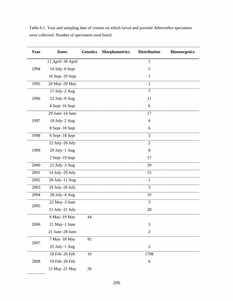
206
Table 6.1. Year and sampling date of cruises on which larval and juvenile Atheresthes specimens
were collected. Number of specimens used listed.
Year Dates Genetics Morphometrics Distribution Bioenergetics
1994
11 April–30 April 1
14 July–6 Sept
5
16 Sept–29 Sept 1
1995 20 May–29 May 1
1996
17 July–2 Aug
7
21 July–9 Aug
11
4 Sept–16 Sept 6
1997
29 June–14 June
17
18 July–2 Aug
4
8 Sept–18 Sept 6
1998 6 Sept–18 Sept 3
1999
12 July–26 July
2
20 July–1 Aug
8
2 Sept–19 Sept 17
2000 21 July–3 Aug 29
2001 14 July–29 July 15
2002 28 July–11 Aug 1
2003 19 July–26 July 3
2004 28 July–4 Aug 10
2005 22 May–3 June
3
15 July–21 July 28
2006
8 May–19 May 44
21 May–1 June
3
21 June–28 June 2
2007 7 May–18 May 92
25 July–1 Aug 2
2008
18 Feb–26 Feb 16
1708
19 Feb–28 Feb
6
12 May–21 May 26
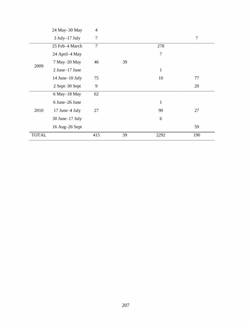
207
24 May–30 May 4
3 July–17 July 7 7
2009
25 Feb–4 March 7
278
24 April–4 May
7
7 May–20 May 46 39
2 June–17 June
1
14 June–10 July 75
10 77
2 Sept–30 Sept 9 20
2010
6 May–18 May 62
6 June–26 June
1
17 June–4 July 27
90 27
30 June–17 July
6
16 Aug–26 Sept 59
TOTAL 415 39 2292 190
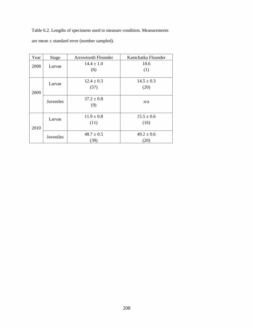
208
Table 6.2. Lengths of specimens used to measure condition. Measurements
are mean ± standard error (number sampled).
Year Stage Arrowtooth Flounder Kamchatka Flounder
2008 Larvae 14.4 ± 1.0 18.6
(6) (1)
2009
Larvae 12.4 ± 0.3 14.5 ± 0.3
(57) (20)
Juveniles 37.2 ± 0.8
n/a (9)
2010
Larvae 11.9 ± 0.8 15.5 ± 0.6
(11) (16)
Juveniles 48.7 ± 0.5 49.2 ± 0.6
(39) (20)
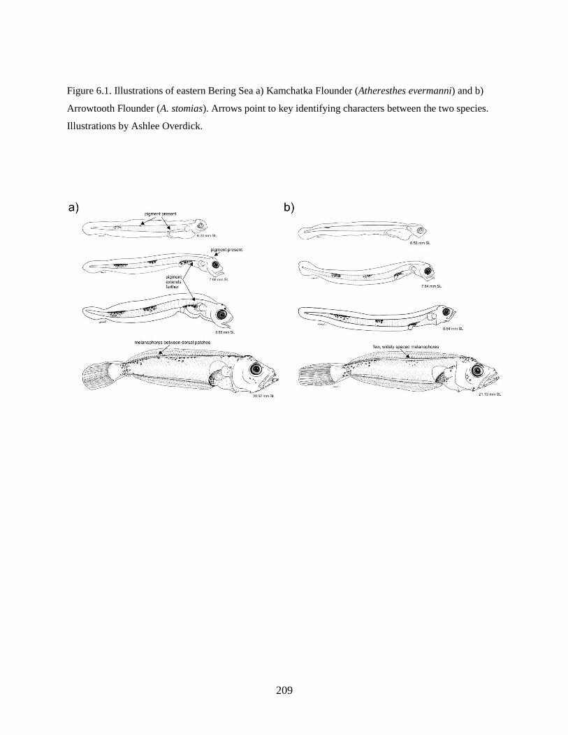
209
Figure 6.1. Illustrations of eastern Bering Sea a) Kamchatka Flounder (Atheresthes evermanni) and b)
Arrowtooth Flounder (A. stomias). Arrows point to key identifying characters between the two species.
Illustrations by Ashlee Overdick.
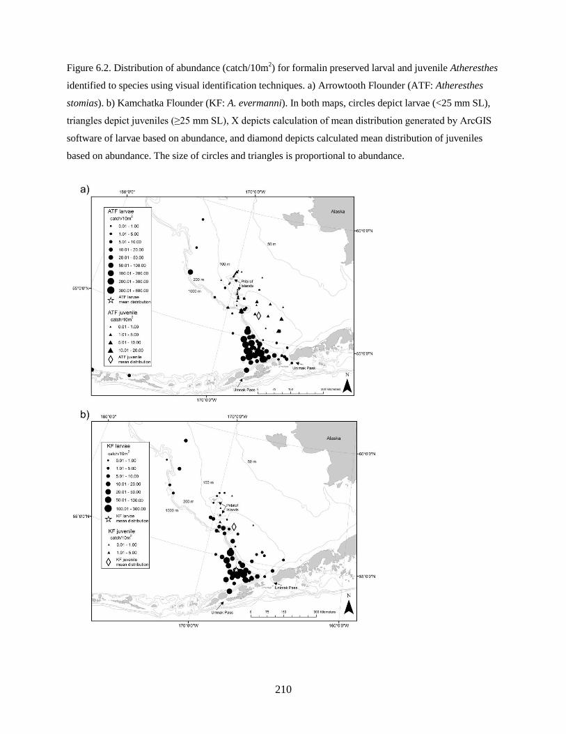
210
Figure 6.2. Distribution of abundance (catch/10m2) for formalin preserved larval and juvenile Atheresthes
identified to species using visual identification techniques. a) Arrowtooth Flounder (ATF: Atheresthes
stomias). b) Kamchatka Flounder (KF: A. evermanni). In both maps, circles depict larvae (<25 mm SL),
triangles depict juveniles (≥25 mm SL), X depicts calculation of mean distribution generated by ArcGIS
software of larvae based on abundance, and diamond depicts calculated mean distribution of juveniles
based on abundance. The size of circles and triangles is proportional to abundance.
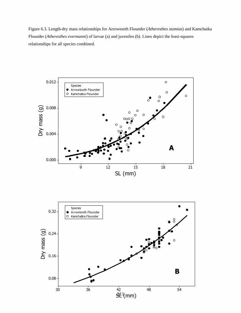
211
Figure 6.3. Length-dry mass relationships for Arrowtooth Flounder (Atheresthes stomias) and Kamchatka
Flounder (Atheresthes evermanni) of larvae (a) and juveniles (b). Lines depict the least-squares
relationships for all species combined.
5448423630
0.32
0.24
0.16
0.08
SL (mm)
Dry
mass
(g)
Arrowtooth Flounder
Kamchatka Flounder
Species
B
211815129
0.012
0.008
0.004
0.000
SL (mm)
Dry
mass
(g)
Arrowtooth Flounder
Kamchatka Flounder
Species
A
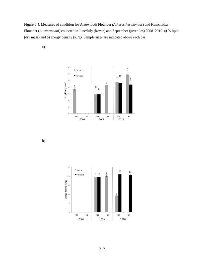
212
Figure 6.4. Measures of condition for Arrowtooth Flounder (Atheresthes stomias) and Kamchatka
Flounder (A. evermanni) collected in June/July (larvae) and September (juveniles) 2008–2010. a) % lipid
(dry mass) and b) energy density (kJ/g). Sample sizes are indicated above each bar.
a)
b)
213
Chapter 7: State of knowledge review and synthesis of the first year of life of Walleye Pollock
(Gadus chalcogrammus) in the eastern Bering Sea with comments on implications for recruitment
Duffy-Anderson, J.T.1*
, Barbeaux, S.1, Farley, E.
2, Heintz, R.
2, Horne, J.
3,
Parker-Stetter, S.3,Petrik, C.
4,5, Siddon, E.C.
2, Smart, T.I.
3,6
1Alaska Fisheries Science Center, National Marine Fisheries Service, National Oceanic
and Atmospheric Administration, 7600 Sand Point Way NE, Seattle, WA 98115, USA
2Auke Bay Laboratories, Alaska Fisheries Science Center, National Marine Fisheries
Service, National Oceanic and Atmospheric Administration, 17109 Point Lena Loop
Road, Juneau, AK 99801, USA
3School of Aquatic and Fishery Sciences, University of Washington, Seattle, WA 98195-
5020, USA
4 University of Alaska Fairbanks, School of Fisheries and Ocean Sciences, 17101 Point
Lena Loop Road, Juneau, AK 99801 USA
5Present affiliation: University of California Santa Cruz, Institute of Marine Sciences,
110 Shaffer Rd., Santa Cruz, CA 95060, USA
6Present affiliation: Marine Resources Research Institute, South Carolina Department of
Natural Resources, Charleston, South Carolina 29422, USA
Citation: Duffy-Anderson, J.T., Barbeaux, S., Farley, E., Heintz, R., Horne, J., Parker-Stetter, S.,Petrik,
C., Siddon, E.C., Smart, T.I. In press. State of knowledge review and synthesis of the first year of life of
Walleye Pollock (Gadus chalcogrammus) in the eastern Bering Sea with comments on implications for
recruitment. Deep-Sea Research II.
214
Introduction
Walleye pollock (Gadus chalcogrammus, previously Theragra chalcogramma, Carr and Marshall
2008; Page et al., 2013) is a sub-arctic gadid found from Japan to the Chukchi Sea to central California.
Walleye pollock (hereafter, pollock) occur over continental shelves, 50 – 300 m depth, migrate in large
schools, and form seasonal spawning aggregations February – June. A major fishery for the species exists
in the Pacific subarctic, where catches have ranged from approximately 0.7 – 1.7 million metric tons in
the Eastern Bering Sea (EBS) and Gulf of Alaska (GOA) since 1984 (Hiatt et al., 2010). First-sale value
for these catches is in excess of $1 billion US per year in the last decade. Fishery products include roe in
the winter and fillets throughout the spring and summer. Not only are pollock of significant commercial
interest, they are also a central component of the food web in the eastern Bering Sea, serving as prey for
fish, marine mammals, and seabirds (Livingston, 1993; Napp et al., 2000; Wespestad et al., 2000; Sinclair
et al., 2008). Since pollock are both economically and ecologically valuable, there is significant interest
in understanding their recruitment, determining how and when recruitment is set, discerning the
associated effects on demographics, and establishing the influences on the overall community structure,
with the ultimate goal of developing appropriate management and conservation strategies for the species.
Recruitment strength in pollock is particularly sensitive to events that occur during the early life phases
because high abundances of small-sized offspring are more vulnerable to mortality than older, more
established life stages (Houde, 1987; 1989).
In an effort to better understand recruitment in pollock it is appropriate to take a careful look at
events occurring during the first year of life. This paper will review the current understanding of pollock
ecology during the first year (spawning to age-1 juveniles), focusing on populations occurring in the EBS.
The EBS was chosen as the system of study as it supports a major pollock fishery and it is experiencing a
shift in atmospheric and oceanographic conditions (Stabeno et al., 2012), which may influence ecosystem
dynamics and function, including pollock recruitment. The review focuses on pollock populations in the
EBS, but makes reference to pollock in other large marine ecosystems in an effort to highlight differences
or expand conceptual thought. This review will also identify areas of research that are needed to improve
our understanding of EBS pollock recruitment, and provide comments on past and current EBS pollock
recruitment paradigms that focus on the first year of life.
We define several early life history terminologies to describe young pollock ontogeny that are
variously used throughout the pollock literature. Here, egg describes the life stage that occurs from
spawning to hatching, also described as the embryonic phase of development (Miller and Kendall, 2009).
The yolk-sac stage begins immediately after hatching and yolk is present for internal nourishment of the
animal. Pollock larvae rely on maternally-provisioned yolk for several days to weeks and yolk exhaustion
occurs when larvae are 5 – 7 mm standard length (SL). Early-stage larvae describe larvae in the
215
developmental period between exhaustion of the yolk sac and flexion of the notochord, a stage also
referred to as preflexion in the literature (Dunn and Matarese, 1987). Late-stage larvae (also referred to as
postflexion) are those stages between notochord flexion (10 – 17 mm SL) and the development of the full,
adult complement of fin rays. The term age-0 juveniles (also, young-of-the-year) refers to individuals with
a full complement of fin rays (transformation typically occurs 30 – 40 mm SL; Brown et al., 2001) that
are less than 1 year old, and age-1 juveniles refers to those individuals that have experienced their first
birthdays.
Collections of pollock during the first year of life in the EBS date from 1979, providing a rich
historical data source from which observations are derived. Ichthyoplankton (eggs and larvae) have been
collected using obliquely towed 60-cm bongo nets, 1-m2 Tucker nets, and 1-m
2 depth-discrete Multiple
Opening and Closing Net and Environmental Sensing Systems (MOCNESS, 333 or 505-µm mesh) by the
National Oceanic and Atmospheric Administration (Alaska Fisheries Science Center) as well as by
numerous academic institutions (University of Alaska, University of Washington, Oregon State
University, among others). Age-0 juveniles have been collected with large rope trawls and with small-
mesh trawls, (both of which typically use a set of trawls doors to open the net) and Methot nets (a fixed-
frame mounted net) towed in the midwater and at the surface. Age-1 pollock have been collected from
bottom trawl surveys and from midwater trawl surveys that are conducted in conjunction with acoustic
surveys. Generally, spring surveys in the EBS collect pollock eggs and early-stage larvae, summer
surveys collect late-stage larvae and transforming juveniles, and autumn surveys collect age-0 juveniles.
There are no overwinter collections and age-1 individuals have been collected in spring and summer the
year after spawning (Table 1). For the purpose of this review, focus will be on ecology of egg – age-0
pollock; age-1 pollock will only be addressed as they pertain to emergent overwintering age-0s.
Review
Oceanographic characteristics of the eastern Bering Sea shelf
The EBS is bordered to the east by the Alaska mainland, to the south by the Alaska Peninsula and
eastern Aleutian Islands, to the west by the Aleutian Basin, and to the north by Bering Strait (Fig. 1). The
continental shelf is very broad (~500 kilometers). Northwest flow is driven by the Alaska Coastal Current
and flow through Aleutian passes (Napp et al., 2000). East-west flow is driven by the Aleutian North
Slope Current. Together these two currents drive flow northward over the shelf. The EBS shelf can be
divided into three bathymetric domains during spring and summer, each with its own characteristic
hydrography (Coachman, 1986). The inner shelf (or coastal domain, < 50 m depth) is weakly stratified
and influenced by freshwater run-off; the middle shelf (50 –100 m depth) is strongly stratified; and the
216
outer shelf (100 – 200 m depth) is an area of intermittent upwelling in the spring and summer, high
productivity, and stratification (Hunt et al., 2002). Ocean thermal conditions are often categorized as
warmer- or colder-than-average (hereafter “warm year” and “cold year,” respectively), based on sea-ice
extent, timing of sea-ice retreat, water temperatures, and the extent of a pool of cold bottom water (Cold
Pool, < 2 ºC) over the middle shelf during the summer (Stabeno et al., 2012). Currents also vary between
cold and warm years; during cold years, currents are predominantly westward, while in warm years
current direction is variable and seasonal, with northward flow during winter and weak flow in other
seasons (Danielson et al., 2012; Stabeno et al., 2012).
Spawning Ecology
Pollock exhibit fidelity to general spawning regions and spawning occurs within predictable time
intervals; however, small-scale spatio-temporal variability exists within broad-scale spawning regions and
known spawning periods that is believed to be dependent on oceanographic conditions. Pollock are
iterative spawners, releasing up to 10 cohorts of eggs each year per individual female (Brodeur et al.,
1996). Maturity occurs at 3 – 4 years of age and female fecundity is in the millions (Hinckley, 1987). In
the EBS, several active pollock spawning grounds have been identified (Fig. 1). Over the shelf, pollock
spawn north of the Alaska Peninsula in the vicinity of Unimak Island in March – April, and proximal to
the Pribilof Islands April – August (Jung et al., 2006; Bacheler et al., 2010). Over the slope, pollock
spawn in the vicinity of Bogoslof Island February – April, although spawning stock biomass in this area
has declined since the early 1990s (Bacheler et al., 2010). Farther north, a potential fourth spawning
aggregation has been identified near Zhemchug Canyon, although the phenology of this aggregation is
unknown (S. Barbeaux, unpublished data). Likewise, a very large, historical spawning aggregation over
the Aleutian Basin, “The Donut Hole” aggregation, was depleted in the 1970s and 1980s, and there
remains only a marginal, remnant population in the basin that does not contribute significantly to the shelf
stock (Bailey, 2013). Spawning stock biomass on the EBS shelf increased substantially in the 1980s due
to an influx of large year classes in the late 1970s and early 1980s (Ianelli et al., 2013). Large recruitment
events continued through the 1980s and 1990s resulting in high spawning stock biomass during this
period. It is believed that strong recruitment and a resultant increase in spawning biomass was due to a
regime shift within the EBS in 1977 favoring juvenile pollock survival (Bailey, 2000; Hunt et al., 2002).
Although a period of poor recruitment and continued fishing from 2001 to 2005 resulted in a decline in
pollock spawning biomass through 2008, recent data suggest that favorable recruitment events in 2006
and 2008 and lower fishing quotas have led to an increasing spawning biomass trend since 2009 (Ianelli
et al., 2013).
Previous work using egg and yolk-sac larval data has suggested a latitudinal cline in pollock
spawning phenology (Hinckley 1987; Bacheler et al. 2010). This phenomenon can also be investigated
217
using pre-spawning data. The commercial roe fishery separates pollock roe into grades of different value;
and hydrated roe can be applied as a proxy for spawning activity. The tonnage of roe recovered by week
and grade was available from the EBS pollock commercial fishery (2001 – 2006) and we combined these
data with weekly centroids of vessel fishing locations. A generalized additive model with the proportion
of hydrated roe as the dependent variable and latitude and week by year as independent variables was fit
using 2-dimensional cubic splines (Wood, 2006). The model explained 62% of the deviance. In general,
hydration, taken as a proxy for spawning, occurred earlier in the south and later in the north, with 50%
hydrated roe occurring 1 – 5 weeks earlier at 54°N than at 58°N latitude (Fig. 2). This was true for all but
two years; in 2004 and 2006 there was little difference in the timing of hydration from north to south.
Interannual differences in timing were also apparent with 50% hydrated roe occurring at 56°N as early as
week 10 (mid-March) (2004 – 2006) and as late as week 14 (mid-April) (2001 – 2002). Results confirm
the latitudinal cline in pollock spawning phenology but also demonstrate interannual plasticity in timing
of spawning, the latter likely related to ocean thermal differences among years examined. Climate-
mediated shifts in spawning phenology can influence density-independent mortality of pre-recruit life
stages through variations in the timing of larval fish production relative to zooplankton production
(match-mismatch hypothesis, Cushing, 1981) or variable dispersal of larvae relative to seasonally-
established oceanographic features. Density-dependent mortality of older stages as a downstream result of
phenological shifts can be manifested through temperature-mediated effects on growth, species
interactions and predation, or juvenile condition.
Early studies suggested the existence of several stocks of pollock within the Bering Sea (Mulligan
et al., 1989; Mulligan et al., 1992; Bailey et al. 1999), though more recent work on genetic differentiation
of pollock populations demonstrated only a weak cline in population structuring from Puget Sound,
Washington, USA, to Funka Bay, Japan (Canino et al., 2005). Nevertheless, Canino et al. (2005)
suggested the existence of self-recruiting populations at moderate geographic scales, though whether
these populations might contribute significantly to the overall population (Smith et al., 1990) remains
unresolved. Other unknowns regarding pollock spawning ecology in the EBS include surprisingly little
spatio-temporal information for how spawning aggregations are formed, or from which spawning locales
resultant larvae are derived. Moreover, there has been work in other parts of the world to show that gadid
fecundities are influenced by environmental factors (Marshall, 2009; Kjesbu et al., 1998), but comparable
studies are lacking for pollock in the EBS. Increased research into the spawning ecology of adults will
help to inform studies on the survival and recruitment of their offspring.
Fertilized Eggs
Eggs appear in the water column in the EBS as early as February in the Bogoslof Island area
(Bacheler et al., 2010). Based on a 17-year time series of ichthyoplankton tows, the peak in the egg
218
production cycle for the EBS population occurs in April and May, with most eggs produced by the
spawning aggregation north of the Alaska Peninsula and Unimak Island (Smart et al., 2012a). Egg
mortality has been estimated on one occasion, in 1977, and was found to be approximately 0.6 d-1
in April
and 0.3 d-1
in May (Jung et al. (2006). Eggs collected in the EBS tend to be larger than eggs collected
from the Gulf of Alaska, and developmental rates at low temperatures are accelerated in the EBS relative
to the Gulf (Blood, 2002) suggesting the EBS population is adapted to colder temperatures associated
with winter ice cover. Normal development occurs at temperatures ranging from 0.4 to 3.8 ºC. Below 0 ºC
development is abnormal and mortality is high.
The timing of peak abundance of pollock eggs occurs earlier in warm years compared to cold
years (Smart et al., 2012b; Table 2), which likely is attributable to either earlier spawning (see Section
2.2) or temperature-dependent effects on hatching and development (Blood, 2002). In the EBS, eggs are
found throughout the water column, occurring to depths as deep as 300 m (Smart et al., 2013), but also
present in the neustonic layer (Waldron and Vinter, 1978). Sampling to document the deepest extent of
pollock eggs in the Aleutian Basin has not occurred, but generally eggs collected over the basin are
deeper than those collected over the continental shelf (Kendall, 2001). Over the continental shelf pollock
eggs are found ≤ 30 m over all domains, but centers of distribution are < 30 m over the shelf and ≥ 100 m
over the slope (Smart et al., 2013).
Larvae
Distribution
Pollock early- and late-stage larvae are found in the vicinity of spawning areas as well as
hundreds of kilometers away from spawning grounds. Over the EBS shelf, larvae are concentrated near
the Pribilof Islands, probably due to local anti-cyclonic circulation patterns (Stabeno et al., 2008) that act
to retain larvae, and north and east of the Alaska Peninsula following transport by the Alaska Coastal
Current (Stabeno et al., 1999) from spawning grounds located in the vicinity of Unimak Island. Very few
late-stage larvae have been collected in proximity to the spawning grounds at Bogoslof Island, despite the
prevalence of yolk-sac and early-stage larvae there (Smart et al., 2012a). This could be the result of low
sampling intensity in this area in late spring when older larvae would be present in the water column, or it
could indicate high mortality or transport away from this island along the Aleutian Island chain (Fig. 1).
Large aggregations of larvae north of the Pribilof Islands have not been documented, but recent evidence
of the occurrence of spawning-condition adult pollock over the outer shelf at latitudes north of 58ºN (S.
Barbeaux, personal communication) suggests that pollock larvae may be concentrated there in late spring.
Increased sampling effort over the outer shelf north of the Pribilof Islands is warranted.
219
Pollock larvae smaller than ~ 15 mm SL can be collected efficiently with several types of
ichthyoplankton nets (primarily bongo or MOCNESS) with mesh sizes as small as 333 µm. Fish longer
than ~ 50 mm SL (age-0 juveniles) are increasingly adept at avoiding capture by plankton nets but can
still be collected by midwater trawls. A problematic area of research on larval pollock occurs at the
juncture in lengths between fish collected efficiently with ichthyoplankton nets, and those sizes that are
collected in small mesh trawls (age-0s, described below). Postflexion larvae 15 – 30 mm SL are relatively
rare in collections by any presently-employed gear types, and constitute a portion of the size population
that is significantly understudied. As such, there is little information on distribution, vertical distribution,
diet, or growth of larvae within this size range.
During cold years in the EBS, centers of distribution of pollock eggs and larvae are located
farther west (outer domain) within the general spawning region than in warm years (middle domain, Fig.
3; Smart et al. 2012b). In cold years, the Cold Pool persists over the southern middle shelf through the
summer months (Maeda, 1977; Reed, 1995), but in warm years, the Cold Pool is restricted to the northern
shelf. Pollock adults avoid water < 2 ºC (Wyllie-Echeverria and Wooster, 1998) and egg development and
hatching is diminished at temperatures ≤ 0 ºC (Blood, 2002). An extensive Cold Pool likely reduces the
available shelf habitat for spawning and for successful embryo development, and can also impact feeding
success, as recent work has shown that zooplankton prey composition is shifted over the middle shelf in
warm years compared to cold (Stabeno et al., 2012; Eisner et al. in press).
Pollock larvae in the EBS are found in the upper 100 m of the water column and depths of
occurrence become shallower with ontogeny (Smart et al., 2013). Yolk-sac larvae are found throughout
the upper 100 m of the water column, and non-feeding stages show no evidence of diel vertical migration.
Late-stage larvae do exhibit diel vertical behavior, with most migration of feeding larval stages occurring
above the pycnocline (~ 30 m in the EBS). Larvae are generally deeper during the day (10 – 40 m) than
at night (0 – 20 m; Fig. 4), and movements are postulated to be dependent on prey levels, light levels, and
predator presence. For comparison, feeding larvae collected form the Gulf of Alaska tended to be deepest
at midday and shallowest at dusk, indicating a crepuscular pattern of movement (Kendall et al., 1987;
Kendall et al., 1994). Depth occurrences of larvae have implications for variability in transport
trajectories, which can ultimately influence the distribution of larvae. Pollock larvae spawned in the
vicinity of Unimak Island are subject to a bifurcated flow, either northward along the 100 and 200 m
isobaths of the EBS, or eastward along the 50 m isobath. Entrainment below the mixed layer depth (~25 –
30 m) increases the likelihood of northward transport (5 – 8 cm s-1
) to the middle and outer shelves, while
entrainment above the mixed layer increases the chance of eastward drift (2 – 4 cm s-1
) and delivery to the
middle and inner shelves (Stabeno et al., 1999). Near-surface entrainment increases exposure to wind-
forced circulation, which has the potential to transport larvae far from nursery areas. Indeed, Danielson et
220
al. (2011) and Stabeno et al. (2012) have both demonstrated that variability in circulation over the EBS
shelf is influenced by changes in wind direction.
Feeding Ecology and Growth
Pollock first-feeding larvae (preflexion stage, 4.5 – 6.5 SL) over the outer shelf primarily
consume copepod eggs and nauplii (Hillgruber et al., 1995). As larvae grow and develop improved
swimming capability and larger mouth gapes, the diets diversify to include copepodites, particularly those
of Pseudocalanus spp. (Strasburger et al., 2014), barnacle cyprids, and euphausiid calyptopis. In 1995 (a
cold year), pollock larvae were found at high densities in mid-May, but prey concentrations were below a
hypothesized critical density of 20 prey l-1
derived for Shelikof Strait, Gulf of Alaska (Napp et al., 2000).
However, critical prey abundances may be lower for Bering Sea larvae due to the cooler temperatures and
lower metabolic rates of larvae. Theilacker and Porter (1995) did not find evidence of starvation at low
prey densities in field-caught larvae in the Bering Sea. More recent work using a flow cytometric assay to
identify starving larvae in the field suggests that pollock larvae collected over the EBS slope and basin
were healthy, though a risk of food limitation (6% of individuals) was noted among larvae collected from
over the adjacent shelf (Porter and Bailey, 2011). Finally, in a recent analysis of the Match/Mismatch
Hypothesis (Cushing, 1981) for pollock larvae and their Pseudocalanus spp. prey, no relationship was
found between an index of spatial mismatch and subsequent recruitment to age-1 (De Forest et al., in
revision). Taken collectively, there is presently little evidence for mass starvation of pollock larvae in the
EBS, though it is cautioned that weak or starving individuals are ready predation targets, making a true
assessment of the food-limited fraction of population difficult to obtain. Larvae collected from the field
are those that are healthy, and best able to avoid predator encounter and capture; mortality has already
removed the others. In order to better assess the role of food limitation among larval pollock, laboratory
studies of critical densities of prey needed over a range of larval sizes and temperatures, with models to
describe consequent metabolism and growth, are required.
Energy allocation strategies in larval and juvenile fish reflect competing physiological demands
of somatic growth versus lipid storage (Post and Parkinson, 2001) and are a response to differing survival
constraints. By maximizing growth and transitioning through the larval period rapidly, larvae minimize
exposure to size-dependent predation during this stage. However, overwinter survival is hypothesized to
be higher in fish that are both larger and have increased lipid reserves, indicating that energy allocation
during the juvenile stage will favor lipid storage while also increasing fish size (Beamish and Mahnken,
2001; Heintz and Vollenweider, 2010). Differing energy allocation strategies for larval (< 25 mm SL) and
juvenile (25 mm < X < 100 mm SL) pollock indicate that distinct ontogenetic stages face different
survival constraints. Larval fish favor energy allocation to somatic growth and development, presumably
221
in order to escape size-dependent predation, while juvenile fish begin to allocate energy to lipid storage in
late summer (Siddon et al., 2013a; Fig. 5).
Historical laboratory efforts to estimate growth suggest rates of 0.1 – 0.7 mm d-1
(Davis and Olla,
1992; Porter and Bailey 2007; Hurst et al. 2013), while field estimates derived from otoliths suggest
nearly 0.4 mm d-1
(Walline, 1985). Dell ‘Arciprete (1992) developed an age-length key from pollock
otoliths collected in the EBS in 1988 and used this to estimate growth rates for 4 – 8 mm larvae at 0.21
mm d-1
. There is some evidence for temperature-mediated growth, a phenomenon that has significant
import to studies of atmospheric and oceanographic thermal variability on pollock. For example, Jung et
al. (2006) used age-length keys to show that larvae collected in 1976 and 1977 (cold years) grew more
slowly (0.12 mm d-1
) than larvae collected in 1979 (warm year, 0.23 mm d-1
), but suggested that
differences were at least partly due to variations in timing of sampling, fish size, and length-specific
growth. Smart et al. (2012b) estimated larval growth rates by assuming that most larvae collected in
consecutive cruises belonged to the same or dominant cohort. They found that growth rates were
dependent on water temperature, and showed that growth rates in cold years tended to be approximately
half those of warm years (0.1 mm d-1
and 0.2 mm d-1
, respectively). Few studies have examined the
consequences of short-term thermal stochasticity or longer, more gradual increases in ocean temperature
on growth rate, and work to incorporate those consequences into a predictive framework is lacking.
Predation
Predation is likely a significant source of pollock pre-recruit mortality in the eastern Bering Sea;
larvae are consumed by vertebrates and invertebrates alike. Most research on invertebrate predation of
young pollock has been done either in the laboratory or in the Gulf of Alaska, where it has been shown
that euphausiids are consumers of yolk-sac larvae (Bailey et al. 1993; Brodeur and Merati, 1993).
Gelatinous macrozooplankton are predators of fish larvae in other marine systems, and their numbers
appear to be increasing in the EBS, in particular the large jellyfish, Chrysaora melanaster (Brodeur et al.,
2002; Brodeur et al. 2008), but we suggest they are not likely to be major predators of pollock eggs and
larvae since the timing of production of jellyfish and larvae is mis-matched, with jellyfish occurring at
small sizes in early spring when larvae are most vulnerable. Vertebrates certainly consume pollock early
life stages. Spawning adult pollock in the EBS are cannibals of pollock eggs (Schabetsberger et al., 1999)
and adult pollock, Pacific cod (Gadus macrocephalus) and arrowtooth flounder (Atheresthes stomias) all
consume pre-recruit pollock (Livingston and Juardo-Molina, 2000; Bailey 2000). The minimum size of
larval pollock in the diets of piscivorous fishes typically ranges from 10 – 20 mm SL, depending on
species of predator. Predation and food limitation (section 2.4.2, above) are likely synergistic factors that
act remove pollock larvae from the population, with predators selectively preying on undernourished,
222
weaker, and slower swimming or poorly-reactive individuals. Rates of predation on weaker individuals
are not well documented but are likely quite high.
Age-0 Juveniles
Distribution
In their first summer, larvae transition to age-0 juveniles prior to reaching 40 mm SL (Brown et
al., 2001). Juvenile pollock have been observed across the southeastern Bering Sea (Winter and
Swartzman, 2006; Moss et al., 2009; Hollowed et al., 2012), with the area around the Pribilof Islands
identified as an essential nursery habitat (Walters et al., 1988; Traynor and Smith, 1996; Brodeur et al.,
1997; Hunt et al., 2002). In that region, age-0s are concentrated in inshore rather than offshore areas,
despite better potential feeding conditions in offshore areas (Ciannelli, 2002). Patchiness in the
distribution of age-0s is common with aggregations ranging in size from meters to kilometers (Benoit-
Bird et al., 2013a). During late summer and early fall Parker-Stetter et al. (2013) found that in 2006 –
2010, age-0 pollock were distributed across the EBS, primarily within the middle and outer shelf regions.
In 2006 – 2008, years that were classified as “average” or “cold” based on sea surface temperature
(Stabeno et al., 2012), high numbers of age-0 pollock were associated with the pycnocline in the upper 30
m of the water column throughout the EBS (Fig. 6, Fig. 10 in Parker-Stetter et al., 2013) as previously
identified in other studies (Bakkala et al.,1985; Swartzman et al., 2002; Moss et al., 2009; Hollowed et al.,
2012). In 2009 and 2010, years that were colder than 2006 – 2008, higher numbers of age-0 pollock
were observed in deep water below the pycnocline (Fig. 6, Fig. 10 in Parker-Stetter et al., 2013). The
presence of age-0 pollock in midwater during summer has previously been observed in the EBS (Miyake
et al., 1996; Tang et al., 1996) and in the Gulf of Alaska (Brodeur and Wilson, 1996) and has been
attributed to survey timing coinciding with the ontogenetic transition from pelagic to demersal habits, and
not due to water column attributes or differences in fish length (Brodeur and Wilson, 1996; Parker-Stetter
et al. in review 1).
Two recent studies (Hollowed et al., 2012; Parker-Stetter et al., in review 2) have evaluated the
horizontal distribution of age-0 pollock relative to physical, biological, and climate factors. Bottom depth
and temperature were important predictors of both near-surface age-0 pollock presence and density in
Hollowed et al. (2012). In contrast, Parker-Stetter et al. (in review 2) found that depth, quantity of
zooplankton prey, and spring winds were important predictors of near-surface age-0 pollock presence and
density. Previous studies have suggested that other factors such as prey abundance and/or predator
overlap (Swartzman et al., 1999; Ciannelli et al., 2002a; Winter and Swartzman, 2006; Winter et al.,
2007), habitat energetics (Ciannelli, 2002b), bottom depth (Brodeur et al., 1999), and temperature
(Brodeur et al., 1999) are also important.
223
Age-0 pollock exhibit diel vertical migration, moving from the pyconcline or deeper into the
near-surface waters at night. Swartzman et al. (2002) concluded that migration patterns were dependent
on stratification, depth, zooplankton prey, and age-0 pollock size. Schabetsberger et al. (2000) suggested
that vertical movements by age-0s were motivated by feeding potential and demonstrated that age-0
pollock and their prey had similar vertical distribution patterns. Bailey (1989) noted that shifts in vertical
distribution of age-0s had significant implications for inter-cohort cannibalism, with age-1 and older fish
feeding on age-0s occurring at similar depth strata.
Feeding Ecology and Growth
Diet of early age-0 juveniles (30 – 50 mm TL) includes small adult copepods (e.g. Pseudocalanus
spp., Oithona spp., and Acartia spp.), euphausiids, amphipods, and chaetognaths (Brodeur, 1998; Brodeur
et al., 2000; Strasburger et al., 2014). Feeding and body condition vary spatially, around frontal regions
and across habitats (Brodeur et al., 2000; Brodeur et al., 2002; Ciannelli et al., 2002a; Ciannelli et al.
2002b; Swartzman et al. 2002; Schabetsberger et al. 2003), and interannually, which appears related to
thermal conditions and associated changes in prey base (Heintz et al., 2013). Age-0 juveniles (30 – 100
mm SL) collected by surface trawls in 2003 – 2006, which were warm years, fed mainly on small
copepods and euphausiids. In 2007 – 2009, which were cold years, age-0 juveniles within the same size
range fed mainly on euphausiids and large copepods (Coyle et al., 2011). This shift is most likely the
result of variation in prey availability rather than feeding ability as juveniles collected in surface trawls in
2004 and 2005 (warm years) were longer with larger mouth gapes than those collected in surface trawls in
2006 and 2007 (an average and a cold year respectively; Moss et al., 2009). A diet shift occurs after
approximately 50 mm TL, and larger-sized age-0 juveniles feed on larger prey including euphausiids and
large copepods (Calanus spp.) (Brodeur, 1998). The switch in diet coincides with the increased
swimming speeds that allow predators to pursue larger, more evasive prey, as well as an increase in gape
size that permits consumption of larger, higher-quality prey items. Moss et al. (2009) suggested that
juveniles 100 – 130 mm TL are piscivorous and cannibalistic during warmer-than-average conditions,
though it remains unclear if any larger pollock in their study might have been small-sized age-1s.
Cannibalism has been documented among age-1 pollock in the EBS (Bailey, 1989; Duffy-Anderson et al.,
2003).
Prey quality and availability relative to juvenile age-0 pollock energetic condition may also
influence recruitment as a function of environmental conditions. Climate effects on prey field
composition (Coyle et al., 2011) have been shown to lead to the consumption of high lipid diets in cold
years (Heintz et al., 2013; Fig. 7). Estimates of total energy in late summer integrate the effects of
climate, diet, growth, and prey abundance and quality at the end of the first growing season. The effects
224
of climate on diet quality and condition of age-0 pollock are consistent with observations of a generally
inverse relationship between late summer sea surface temperatures and survival (Mueter et al., 2011).
Prey resources for age-0 juvenile pollock decline in autumn and reduced foraging opportunities
coupled with near-freezing temperatures during winter heighten the importance of body size and
physiological condition prior to winter onset. In high latitude systems, winter is a period of low light, cold
temperatures, and reduced prey availability, and is therefore a significant source of mortality and a
determinant of recruitment success of marine fishes (Hurst, 2007a). Availability of lipid-rich prey during
this period is important as age-0 pollock face severe energy deficits during winter (e.g., Sogard and Olla,
2000). The window of time during which pollock can provision themselves with lipid occurs between the
completion of metamorphosis in early August and the onset of oceanographic winter (Wilson et al., 2011;
Siddon et al., 2013a). Those individuals that can consume high lipid prey during this critical period are
expected to survive winter better than individuals consuming leaner prey. The energetic status of age-0
pollock in late summer is recognized as a predictor of age-1 abundance during the following summer in
the EBS (Heintz et al., 2013). Therefore, late summer (July – September) represents a critical period for
energy storage in age-0 pollock, and subsequent energy levels provide an early metric for the prediction
of overwinter survival and recruitment success to age-1.
Predation
Age-0 juvenile pollock are preyed upon by a wide variety of predators. Age-0s <100 mm SL are
eaten by older pollock, yellowfin sole Limanda aspera, arrowtooth flounder, and Pacific cod (Livingston,
1993). Most consumption by adult pollock and arrowtooth flounder on age-0 pollock occurs late in the
day (Lang et al., 2000). Some authors have contended that cannibalism is the most important source of
mortality of age-0 juvenile pollock in the EBS (Livingston and Jurado-Molina, 2000). Hunsicker et al.
(2013) found that arrowtooth flounder population abundance and temperature synergistically affect the
spatial overlap of predator (arrowtooth flounder) and prey (pollock) suggesting that the magnitude of the
primary source of predation of young pollock, arrowtooth flounder, may shift if projections of a warmer
EBS become reality. Predation (and cannibalism) by fishes has been hypothesized to be the most
significant contributor of age-0 juvenile mortality (Bailey, 1989; 2000; Livingston and Jurado-Molina,
2000) and an important regulator of overall recruitment, but recent work suggests a significant role for
feeding, body condition, and overwinter survival.
Marine birds and mammals constitute a significant, although less pronounced, source of predation
on juveniles (Livingston, 1993). Benoit-Bird et al. (2013b) showed that predation on age-0 juvenile
pollock by seabirds and northern fur seals (Callorhinus ursinus) was dependent not on overall prey
biomass, but on small-scale prey density.
225
Models
Biophysical Models
Several generations of biophysical models have been used to explain factors affecting distribution
and abundance of young pollock over the Bering Sea shelf. Spatially explicit, coupled biological-physical
models simulate dispersal of the early life stages and the biological processes that occur during this period
(Table 3). One of the first biophysical models of the early life stages of pollock in the Bering Sea was
used to test the effect of advection and sub-grid scale diffusion on the distribution of larvae (Walsh et al.,
1981). The two-dimensional (2-D) physical model tracked distribution of two life history stages, non-
feeding and feeding larvae, in the vicinity of Unimak Island. The results of model simulations supported
the idea that spawning date affected the drift trajectory and mortality of individuals.
Later, 2-D float-tracking models developed in the 1990s described near-surface wind-driven
transport of pollock larvae in the EBS, but they contained no biological component (Wespestad et al.,
1997; Wespestad et al. 2000) and pollock larvae do not typically occur at the surface. These models were
used to examine how surface advection during the early life stages related to recruitment success by
characterizing annual circulation as good or bad, with the effects of circulation on recruitment feeding
into a stock assessment model for pollock. This model was further used to analyze how wind-driven
transport affected the distribution of juvenile pollock in relation to the distribution of adults (Wespestad et
al., 2000). Strong year classes, which often occurred in warm years, coincided with transport of early life
stages to the north and onshore, which separated juveniles from adults. Average year classes
corresponded with transport to the NW along the shelf, whereas weaker year classes resulted from little
transport, which left juveniles on the outer shelf near adults.
A more complex biophysical model has recently been used to examine stage-specific, 3-D
transport trajectories of pollock larvae over the EBS (Petrik et al., in press). The physical model used a
version of the 3-D Regional Ocean Modeling System (ROMS) for the North East Pacific (NEP;
Curchitser et al. 2010; Danielson et al., 2011) that included the EBS domain. Daily averages of velocity,
diffusivity, and temperature were generated with ROMS-NEP6 and used to force the particle-tracking,
biological model, TRACMASS (Döös, 1995), which simulated the development, growth and vertical
behavior of pollock eggs and larvae. Results showed that shifts in spawning location, rather than changes
in current patterns or temporal shifts in spawning time, contributed most to spatial shifts of larvae and
juveniles observed over the EBS shelf. It was concluded that field-observed differences in distributions of
eggs and larvae over the continental shelf between warm and cold years most likely occur because adults
modify their use of spawning habitat in response to changes in the presence and extent of sea ice. Direct
observations from the field are necessary to verify this hypothesis.
226
How has understanding of pollock early life ecology been shaped by biophysical modeling
studies? Until only recently, physical models were primarily 2-D and incorporated little or no pollock-
specific biology. Larvae were considered passive particles since there was limited ability to account for
species-specific variations in physiological and behavioral characteristics within the model framework.
While early models certainly had utility as predictive tools for evaluating horizontal dispersal relative to
mean flow, and they had the advantage of modest computational requirements, their value for enhancing
understanding of pollock biology was significantly hampered by the inability to account for species-
specific attributes that have the potential to influence, or even change, the dispersal outcome. The legacy
of biophysical modeling in the study of pollock biology has been vastly improved since the development
of spatially-explicit, 3-D circulation models coupled to Lagrangian particle tracking and behavioral
models, and they have the potential for further advancement with the more recent development of full life
cycle models than span generations (reviewed by Lett et al., 2010). As they exist now, biophysical
models of pelagic fishes, inclusive of pollock, provide powerful tools with which to evaluate long-term
shifts in growth, distribution, and recruitment. Use of biophysical models of pollock in the Bering Sea in
recruitment prediction scenarios is forthcoming (C. Petrik and F. Mueter, personal communication), but
remain regional and single species.
Trophic Models
Trophic models have been developed that link age-0 pollock juveniles with other components of
the EBS ecosystem in an effort to determine energy flows, relative importance, and consequences on
pollock survivorship and subsequent recruitment. All too often however, these models minimize large
portions of the first year period, typically egg and larval, favoring to model those life history phases as
dispersed propagules rather than treating them as part of the larger trophic framework. This approach
assumes that primary sources of larval mortality are density-independent, an assumption that is
increasingly turning out to be biased. While evidence for mass starvation of pollock larvae in the Bering
Sea is equivocal (section 2.5.3, above), the role of predation upon larvae weakened by poor nutrition
should not be overlooked. For decades predation has been acknowledged to be a major source of
mortality among marine fish larvae (Hunter et al. 1981; Bailey and Houde 1989; Leggett and Deblois
1994; Houde, 2002; Gallego et al. 2012), and predation likely plays a critical role in structuring age-0
pollock cohort strength. Knowledge of the links and energy pathways that put larvae at risk of predation,
including prey availability, foraging capability, feeding, temperature, biochemical condition, swimming
competency, and sensory development provides critical mechanistic understanding of how young pollock
interact with the environment, which factors are strongly limiting, and over what developmental stages
recruitment controls are likely to act. Given the importance of the first year of life to recruitment success,
we encourage development of trophic models that are specifically focused on the first year to better
227
understand mechanisms regulating early life survival and connections between vulnerable young fish and
the broader ecosystem.
Despite the limitations described above, trophic models have been successful in identifying
energy flows from the age-0 juvenile phase forward. Earlier food web models that included young
pollock in the EBS took the form of mass balance food web approaches, such that flow of juvenile age-0
biomass entering and leaving the ecosystem was tracked and accounted for, allowing biomass loss or gain
by the system to be realized (Aydin et al., 2007). Mass balance models achieved success in identifying
and quantifying key sources of juvenile pollock mortality in the EBS (cannibalism), determining the
sensitivity of pollock to fluctuations in prey availability, and identifying key energy flows to upper
trophic levels that rely on juvenile pollock production.
Physiological trophic modeling approaches have been applied in the EBS to test the hypothesis
that variability in pollock growth and survival is structured, in part, by climate-driven, bottom-up control
of zooplankton composition. To this end, the broadly applied Wisconsin bioenergetics modeling approach
(Kitchell et al., 1977; Ney, 1990) has been adapted for pollock (Ciannelli et al., 1998; Mazur et al., 2007;
Holsman and Aydin, in review). The spatially-explicit model estimates temperature- and weight-specific
consumption and assesses changes in predicted growth under varying prey or climate conditions. Model
results suggest variability in age-0 pollock growth rates relative to hydrographic features which may
influence prey availability and food supply (Ciannelli et al., 2002), and pronounced, thermally-induced
changes in the relative foraging rates and daily ration of arrowtooth flounder and Pacific cod (Holsman
and Aydin, in review).
A mechanistic, 3-D individual-based trophic model (IBM) has also been developed and applied to
age-0 juvenile pollock to predict growth over geographic area. The IBM, based on that of Kristiansen et
al. (2009), predicts growth using a mechanistic prey selection component that simulates the feeding
behavior of age-0 juvenile pollock on zooplankton. The simulated feeding ecology depends on age-0
development (e.g., swimming speed, gape width, eye sensitivity) and vertical behavior, prey densities and
size, as well as light and physical oceanographic conditions. This approach has been used to examine
mechanisms underlying observed differences in juvenile pollock energy content between warm and cold
years in the EBS (Siddon et al., 2013b). Model results revealed that poor growth conditions resulted from
spatial mismatches between juvenile pollock and spatial hot spot areas that are conducive to growth, and
were correlated to interannual variations in pollock recruitment.
Most recently, efforts have focused on fully integrated model frameworks, in which output from
one model feeds another in a vertical suite of model hierarchies. Efforts such as the Bering Sea Integrated
Ecosystem Research Program (http://bsierp.nprb.org/) have provided a platform for the development of
228
linked biophysical- energetics models that offer the opportunity to evaluate spatial predictions of fisheries
based on Intergovernmental Panel on Climate Change scenario inputs (2000–2050). At its base, hindcast
(1970 – 2005, for model validation) or forecast climate scenarios force a 3-D, 10-km resolution physical
oceanographic model (ROMS) that contains an embedded Nutrient-Phytoplankton-Zooplankton-Detritus
(NPZD) component. Upper trophic level dynamics are modeled through the age-length based
bioenergetics model FEAST (Forage-Euphausiid Abundance in Space and Time), which adopts a layered
landscape approach to modeling foraging, growth, movement, and survival of 15 distinct fish groups (I.
Ortiz, personal communication). FEAST provides two-way feedback between the NPZD model and the
fish groups so that it can capture bottom-up and top-down influences on ecosystem dynamics.
Finally, multi-species stock-assessment models (MSMs) quantify the indirect effects of fisheries
harvest on populations and evaluate management trade-offs for fisheries that target several species.
MSMs include population dynamics models for each stock and link these through annual predation
mortality rates (Jesus-Molina and Livingston, 2004). Holsman et al. (in review) recently used this
approach to demonstrate that interactions between fishing pressure and Pacific cod and arrowtooth
flounder predation on age-0 juvenile pollock strongly influence adult pollock population biomass. These
authors have clearly shown that trophic interactions and harvest rates affect biomass estimates, so the
ultimate goal would be to incorporate this information into stock assessment.
Model Caveats
It should be cautioned that the output of any model is only as sound as the input data used in its
parameterization and the observational data used in model validation. Therefore, while model efforts
have certainly helped researchers understand factors influencing pollock connectivity, trophic
interactions, phenology, distribution, survival, and recruitment in the EBS, their value remains contingent
upon the supporting laboratory and fieldwork that are indispensable for model success. In the Bering Sea,
key observational data are lacking in several critical areas, which compromises the value of hypothesis
testing using a model context. One crucial consideration is the need for stage-specific information, given
that different developmental stages have varied physiological requirements, behaviors, and ecological
constraints that potentially influence model outcomes. Basic information by developmental stage that is
wanting includes robust temperature- and size-dependent growth rates, information on prey preferences,
consumption rates as a function of prey type, prey biomass, and temperature, assimilation rates, resting
metabolism as a function of size and temperature, and maximum growth rates under unlimited food
conditions. In order to be fully operative, studies must be conducted across the range of temperatures
experienced during the larval period and with prey sources that represent the natural mix of zooplankton
encountered in the field.
229
Of course, the argument could be made that rich data sources exist for congeneric species,
particularly Atlantic cod, Gadus morhua, which could be used as proxy data in model development, or
that field work from other ecosystems, namely from studies of pollock from the Gulf of Alaska, are ready
substitutes for the data-poor Bering Sea. This tactic should be approached with caution, as species-
specific or regional differences in physiology, development, ecology, and behavior all have the potential
to influence model-predicted outcome. An exercise conducted for the purposes of this review highlights
these constraints. Growth rates (mm d-1
) across temperatures were derived from the literature for gadids
from the Bering Sea, Gulf of Alaska, Funka Bay, Gulf of Maine, and Norwegian Sea and plotted relative
to one another. Derivations were based on either original empirical models fit to laboratory estimates or
otolith derived estimates of age/length, or growth rates back-calculated from field-observed lengths (or
weights converted to length using published algorithms). Results show significant differences in
temperature-dependent growth among species, within regions, and across ecosystems (Figure 8A).
Moreover, comparative age-length plots (Figure 8B) show that growth trajectories vary greatly among
species examined, with several species reaching asymptotic size thresholds at temperatures that are well
within the optional thermal range for others.
Other examples of subtle but meaningful differences include regional differences in egg
buoyancy (Kendall, 2001), which can impact drift rate and trajectory in depth-specific currents, durations
of larval development and the pelagic larval period (Auditore et al., 1994), which affect time in the
plankton and dispersal potential, vertical movements of juveniles in response to environmental cues
(Brodeur and Wilson, 1996; Smart et al., 2013), which influence growth and survival, and predation risk
(as reviewed in Ottersen et al., 2014) as it has the potential to control predicted recruitment biomass
(Hunsicker et al., 2013). Use of data derived from other sources may be necessary at times, such as when
model predictions are the only option for making fisheries management decisions despite incomplete
understanding. In these cases, careful consideration and thorough vetting a must when results are to be
applied in a predictive framework.
Recruitment paradigms
The term recruitment generally refers to the age at which a fish species becomes vulnerable to the
fishery; in the case of pollock this is typically age 3 – 4 (Ianelli et al., 2013). To ecologists however,
recruitment is a general term that describes survival from one phase in the life cycle to another. For the
purposes of this work, we use recruitment to refer to the survival of an annual cohort to the second year of
life (age-1). Here we review the recruitment hypotheses that center on the cohort success of pollock
during the first year of life, focusing on hypotheses that affect transport, variability in nutritional status,
and vulnerability to predation, to better understand the role of fish early life history in population
fluctuation of pollock in the EBS.
230
Transport
The Transport-Cannibalism Hypothesis predicts that strong pollock year classes are produced in
years that support high rates of juvenile transport away from the adult habitat (Wespestad et al., 2000;
Yamamura, 2005; Sakurai, 2007), reducing the distributional overlap of age-0 pollock with cannibalistic
adults. This hypothesis assumes that vertical distributions of predators and prey are similar as well, which
has been shown to be the case among cannibalistic age 1+ pollock in the EBS (Duffy-Anderson et al.,
2003). Cannibalism of young pollock in the EBS is indeed high; Aydin et al. (2007) estimated that
cannibalism accounted for nearly 40% of the total mortality of juvenile pollock in the 1990s. The
Transport-Cannibalism hypothesis assumes that 1) juvenile distribution patterns are determined by
passive drift of eggs and larvae in the upper water column, and 2) warmer-than-average ocean conditions
are associated with transport to the middle and inner shelves where the presence of adults is reduced.
Recent evidence suggests eastward distributional shifts in pollock eggs, larvae, and early juveniles in
warm years (Smart et al., 2012b), but concomitant eastward shifts in the distribution of adults (Kotwicki
et al., 2005) may, in fact, maintain the overlap between adults and juveniles. Generally however, we find
that the Transport-Cannibalism Hypothesis retains its applicability to the present. The EBS is broad, flat,
and relatively homogeneous, providing little landscape refuge for vulnerable age-0 pollock to shelter from
large, cannibalistic adults. Empirical and theoretical evidence (Danielson et al., 2012; Stabeno et al.,
2012; Wilderbuer et al., 2013) document the differential oceanographic currents that act to disperse
larvae, and studies have shown that overlap indices of adult and juvenile pollock can explain up to 50% of
recruitment variability (Mueter et al., 2006). Environmental conditions can modify the strength of
predator-prey overlap as has been shown between predatory arrowtooth flounder and age-1 pollock
(Hunsicker et al., 2013), but the interplay of spatial co-occurrence and top-down predation clearly
continues to measurably modify juvenile pollock survivorship and subsequent recruitment.
The Recruitment Routes Hypothesis was developed to understand recruitment variability in the
Oyashio ecosystem off of Japan (Suzaki et al., 2003), but may have application to the Bering Sea. This
hypothesis explores the link between physical oceanographic shifts and changes in distribution and
abundance of pollock, suggesting that differential transport of eggs from spawning grounds underlies
shifts in recruitment success. These authors proposed that when the southward flow of the Oyashio
Current was strong and nearshore, successful transport to the Doto nursery resulted in average or good
recruitment due to the presence of feeding conditions that favor growth potential. When the Oyashio
Current was weakened and offshore, poor year classes were observed. The Recruitment Routes idea has
been applied to the EBS to describe factors that contribute to the fluctuation of flatfish populations
(Wilderbuer et al., 2002), and is currently under investigation for pollock in the EBS (Petrik et al., in
prep.).
231
Nutrition and condition
The Production-Competition Hypothesis predicts that strong year classes in the EBS are produced
in years with strong storm activity in the summer (Bond and Overland, 2005) based on the observation
that four out of five high recruitment years from 1977 to 2000 included warm and windy summers.
Storms that occur after the establishment of summer stratification promote mixing of nutrients from
below the thermocline into the euphotic zone where nutrients enhance a prolonged period of primary
productivity (Sambrotto et al., 1986; Whitledge et al., 1986). Prolonged productivity then may be
converted to high availability of preferred prey for larval pollock, reducing competition. Indeed, increased
abundances of late larvae have been associated with moderate to vigorous summer wind mixing, and high
abundances of early juveniles were associated with high summer wind mixing from 1988 – 2008 (Smart
et al., 2012a). Increased abundances of feeding larvae and early juveniles were associated with high
concentrations of copepods in these years as well. However, recent warm and windy years (2003, 2004,
2005) have not produced strong year classes (Coyle et al., 2011) and not all warm and windy years prior
to 2000 produced strong year classes (Bond and Overland, 2005). The Production-Competition
Hypothesis is probably only partially valid in that bottom-up forcing plays a role in pollock larval
survivorship, but agents of mortality acting between the larval stage and recruitment to age-1 can modify
or even nullify effects. As an example, Gann et al. (in revision) found that a weak year class of pollock
was derived from 2007, despite lower trophic level conditions that initially appeared favorable for
recruitment, due to weak summer wind patterns that led to poor missing, high stratification, and low
nutrient replenishment.
The Oscillating Control Hypothesis (OCH; Hunt et al., 2002) predicts that the EBS ecosystem
alternates between primarily bottom-up control in cold phases and primarily top-down control in warm
phases. Warm years are predicted to be favorable to pollock recruitment. This hypothesis is based on the
impact of interannual variation in the timing of sea-ice retreat on spring and summer temperature
conditions and the extent of the Cold Pool, similar to the Production-Competition Hypothesis. The OCH
diverges from the Production-Competition Hypothesis in that zooplankton production is not tied to the
onset or persistence of the spring bloom, but rather zooplankton production is directly tied to the water
temperature in which zooplankters are grazing on the spring bloom. During cold periods with late ice
retreat, there is an ice-associated spring bloom while during warm periods there is an open-water spring
bloom, so prey availability for zooplankton is not necessarily limiting in either scenario. In cold periods,
however, zooplankton grazing rates, subsequent growth rates, and the onset of reproduction are
diminished by temperature (Walsh and McRoy 1986; Huntley and Lopez 1992), thus reducing availability
of zooplankton prey to larval fish. Biomasses of copepods that serve as the primary prey items for pollock
larvae (Calanus marshallae, Pseudocalanus spp., and Acartia spp.) were reduced in the cool springs of
232
1980 and 1981 relative to the warm springs of 1997 and 1998 (Stockwell et al., 2001; Napp et al., 2002).
The hypothesis predicts that several successive warm years producing strong year classes of fish
contribute to a build-up on the pollock population in the EBS. However, limitations of the hypothesis
were realized after the failure of several successive warm-year year classes (2001 – 2005), and the
success of several pollock year classes produced from a series of cold years (2006 – 2009). A recent
modification (Hunt et al., 2011) to the original OCH suggests a more dynamic interplay of temperature,
sea ice, copepod production, and young pollock than originally conceived, and predicts that cold years are
favorable to pollock recruitment. In the revised view, early ice retreat and warm waters still enhance
primary, and in turn secondary, production contributing to large numbers of age-0 pollock in spring and
summer. However, a lack of large, lipid-rich copepod species during warm years is a factor in poor body
condition of age-0 pollock in autumn, contributing to high overwinter mortality and poor survival to age-
1.
The Critical Size Hypothesis is similar to ideas outlined in the OCH but also recognizes the need
for juvenile fish to store energy prior to winter (Beamish and Mahnken, 2001; Heintz et al., 2013). The
OCH states that recruitment of a cohort depends on both the size and diet of the fish during the period in
which they provision themselves prior to their first winter. The time at which larval transformation is
complete is a direct function of temperature (Smart et al., 2012b), so under warm spring and summer
conditions age-0 pollock should complete larval development early, increasing the length of the
provisioning period. However, fish must also encounter abundant and energy-rich food in order to meet
the metabolic demands of growth while maximizing energy storage (Siddon et al., 2013a). Actively
finding food is particularly important for smaller fish with reduced energy reserves compared to a larger
fish with ample stored energy and reduced incentive to search for prey. Failure to encounter food of
sufficient quality will produce fish entering winter with lower levels of stored energy. Therefore, the
conditions that maximize survival beyond the first summer of life are those that lead to early larval
transformation, production of abundant energy-rich prey, spatial overlap between pollock and prey, and
maximal energy storage in the form of lipids.
While the body of evidence supporting the link between pre-winter condition and survivorship is
building (Sogard and Olla, 2000; Heintz and Vollenweider, 2010), critical questions remain unanswered
that complicate the two hypotheses outlined above. Laboratory studies rearing larval pollock at low
temperatures (<2 ºC) indicate that pollock not only survive extreme thermal conditions, but are capable of
growth during the winter (T. Hurst, personal communication). This observation is supported by results
from spatially-explicit bioenergetics models of young-of-the-year pollock in the Bering Sea suggesting
that age-0 juveniles grow at temperatures as low as 2 ºC (Ciannelli et al., 1998; Siddon et al., 2013a). If at
least some growth can occur over the winter, it may be possible for overwintering fish to compensate for
233
poor initial condition. Metabolic adjustments may be possible, and certainly behavioral thermoregulation
is documented for overwintering pollock (Sogard and Olla, 1996; Hurst, 2007b), leaving open the
possibility that age-0s could offset some of the expense of small initial body size or poor condition.
Additionally, in the absence of good in situ measurements, it is difficult to know how much spatial
plasticity of food resources exists overwinter, which can potentially offer low, but growth-sustainable,
levels of localized prey resources to small age-0s. Of course, though small fish have reduced metabolic
requirements they also have lower overall energy reserves, so the potential to deplete energy stores faster
than larger pollock remains. Nevertheless, small, winter-emergent juvenile pollock are collected in
spring, indicating that survival of small fish does occur overwinter. Finally, the influence of winter
severity on survivorship has not been investigated, but mild winter temperatures could preclude winter
starvation if sufficient food resources persist. In light of these unresolved issues, the risk of overwinter
mortality due to small body size or poor condition needs further investigation.
The Gas Tank Hypothesis (Sigler et al., in review) builds from the Critical Size Hypothesis to
recognize that timing of production across trophic levels is critical to pre-winter conditioning success in
pollock during the first year of life. This theory maintains that timing of the spring phytoplankton bloom
is central to phytoplankton-zooplankton-pollock energy transfer, but is careful to recognize that dynamics
in summer and autumn, particularly temperature-metabolic requirements and predation, remain important
to pre-recruit production. Moreover, the hypothesis maintains that production is also dependent upon
spatial co-occurrences of phytoplankton-zooplankton-pre-recruit pollock, and that successive warmer-
than-average or colder-than-average conditions over the EBS shelf influence overall trophic control of
recruitment success to age-1.
Predation
Conceptual models of pollock recruitment as related to predation impacts on age-0s have been
best developed in the Gulf of Alaska. The Shifting Control Hypothesis (Bailey, 2000) suggests that
control of pollock recruitment in the Gulf shifted from bottom-up control of abiotic parameters acting on
feeding and survival of pollock larvae in spring, to top-down control by large piscivorous predators, most
notably arrowtooth flounder and Pacific cod feeding on age-0 pollock in summer and autumn. Increases
in biomass of these and other piscivores, coupled with the Gulf of Alaska’s narrow continental shelf and
constricted landscape geography that acts to bring predators and pollock into close proximity, makes this
a feasible hypothesis in the Gulf system but less likely to exert population level control in the EBS.
Biomass of predator species is increasing in the EBS, but the broad continental shelf allows for greater
spatial separation of predators and prey, making top-down predation control by piscivores less
problematic unless factors act to bring predators and prey into close proximity (ex: Cold Pool
presence/absence, Transport Cannibalism Hypothesis). Multi-species modeling efforts in the EBS suggest
234
that top-down recruitment control is possible, but caution that it is temporally variable and dependent
upon predator population levels (Livingston and Jurado-Molina, 2000).
A corollary to the Shifting Control Hypothesis is the Climate-Biology Hypothesis (Ciannelli et
al., 2005). In this refinement of the original Shifting Control idea, the authors proposed that the dominant
mechanisms of juvenile pollock mortality (predation) in the Gulf of Alaska could change over contrasting
climate regimes, suggesting a dynamic interplay of climate and predation pressure. They demonstrated
that during ecosystem phases characterized by elevated sea surface temperatures and high predation on
juvenile pollock, pollock recruitment variability and abundance were below average. In contrast, periods
characterized by low temperatures and relaxed predation were associated with high pollock abundance
and high population variability. The recognition of the interplay of physical and biological forcing factors
on pollock recruitment is not unique, but has important implications for the management of the species in
the Gulf of Alaska and elsewhere.
Data Gaps
Even after nearly 40 years of active research, basic information on pollock early life dynamics in
the EBS remains unresolved. Researchers have disentangled certain aspects of the complex ecology of
young pollock, though changes in climate, oceanography, trophic structure, and food web dynamics act
synchronously to interrupt, modify, or break down known relationships, prompting a continuing need to
re-evaluate and redefine conceptual frameworks. The following sections identify gaps in knowledge of
pollock early life ecology, and reflect on the variables that are appropriate for continued monitoring as
they may either be uniquely influenced by changing ecosystem dynamics or exert disproportionate control
on pollock recruitment.
Spawning location
The vast geographic area over which pollock spawning grounds are located, coupled with the
large spatial discontinuities in their locations, make comprehensive sampling of putative pollock
spawning locations in the Bering Sea extremely difficult. Moreover, logistical constraints of sampling
during late winter and early spring when storms are frequent and sea ice is present complicate complete
pre-spawning and spawning sampling. Recent work (De Robertis and Cokelet, 2012) suggests that
pollock shift their distribution away from areas of cold water and extensive ice cover, indicating spawning
under the ice is probably minimal. There is indirect evidence of spawning north of 60 ºN latitude over the
outer shelf in the vicinity of Zhemchug Canyon (see section 2.2), but direct evidence is lacking. Critical
questions linger: Does spawning area expand and contract interannually with variable thermal conditions?
Does spawning habitat become fragmented by the presence of the Cold Pool? What happens to spawning
activity when the preferred spawning area is covered by ice? Pollock in the BS exhibit broad-scale
235
spawning site fidelity, but do they move into deeper water over the basin where temperatures are warmer
and sea ice is lacking, thus spawning in locations where currents are less conducive to on-shelf transport
of offspring? Continued monitoring of spawning populations, complemented by long-term observations
of egg and early larval distributions, is critical to elucidating environmental tolerances of adult pollock
during spawning, and potential effects on recruitment.
Climate-induced variability in timing of spawning has been suggested in several studies but
questions remain. Predominant currents in the EBS are seasonally altered due to the early spring
establishment of the Inner Front along the Alaska Coastal Current (Stabeno et al., 1999; Kachel et al.
2002), which has major implications for transport and distribution of larvae and ultimately for spatial
distribution of age-0 juveniles. Pollock adults that spawn in the vicinity of Unimak Island produce larvae
that are entrained in one of two major flows, the cross shelf flow of the Alaska Coastal Current that
delivers propagules over the southeastern middle shelf, and the northward flowing current along the 100
and 200 m isobaths (Fig. 1) delivering larvae over the outer shelf. Set up of the Inner Front typically
occurs in late spring (Kachel et al., 2002), a month or more after the presumed spawning time for pollock
in that vicinity (March). Shifts in spawning time relative to establishment of the Inner Front have the
potential to affect the proportion of offspring that are delivered to the middle and outer shelves.
Some progress can be made in addressing the questions posed above with regard to spawning
ecology by examining long-term variations in maturity scales and by examining shifts in distributions of
eggs. Collections of ovaries from annual pre-spawning acoustic surveys have suggested differences in
timing of gamete development with thermal regime (Smart et al, 2012a) and differences in spawning time
between warm and cold periods in the EBS have been inferred through examination of timing of peak
abundances of pollock eggs (Smart et al., 2012b). These approaches suggest that spawning can be
delayed by up to a month during cold years. In addition, multi-year surveys of egg distribution can
provide indirect evidence for spatial shifts in spawning areas due to climate and oceanographic shifts, as
has been shown for Arcto-Norwegian cod (Sundby and Nakken, 2008).
Finally, until now we have not had the technology to localize the natal area for any particular
juvenile pollock collected at sea. This information would be extremely valuable in clarifying stock origin,
resolving the degree of mixing among Bering Sea source areas (Bogoslof, Unimak, Pribilof, Zhemchug),
and answering source-sink connectivity questions. Analysis of otolith elemental composition could help
to resolve these issues since otoliths incorporate trace metals into their growth rings that can be related to
environmental conditions at the time of the growth period. Otoliths have been used to resolve natal
origin, connectivity, and nursery habitat for anadromous species (Thorrold et al., 1998; Kennedy et al.,
2002), reef fishes (Ruttenberg et al., 2008), and flatfishes (Cuveliers et al., 2010), but the effort for
pelagic fishes has been complicated by the temporal scale of residency relative to dispersal potential
236
(Gillanders, 2011). However, recent work using gadoids shows some promise. Thorisson et al. (2010)
were able to trace natal areas of age-0 Atlantic cod in a year with limited oceanic mixing, DiMaria et al.
(2011) determined that elemental signatures in larval Pacific cod (Gadus macrocephalus) could reflect
thermal as well as chemical variations in rearing water, and a pilot study using pollock collected from the
Gulf of Alaska indicated that broad-scale geographic differences in residency may be resolved among
age-0s (Fitzgerald et al., 2004). These approaches, if successfully applied in the EBS, would be extremely
valuable to begin addressing questions such as, “Which source areas contribute significantly to the overall
population biomass?”; “To what degree does pollock input from the Gulf of Alaska affect EBS population
structure?;” “What are the connectivity links, rates, and routes between larval, juvenile, and adult fish?;”
and “How much local recruitment is there?”. The EBS, with its broad, homogenous seascape and well-
mixed water column during the pollock spring-spawning period present challenges, but continued efforts
are encouraged.
Ageing
Ambiguities in ability to accurately assign daily ages to larvae and age-0 juveniles from otoliths
have hampered early life studies of walleye pollock in the EBS. Determining ages of larval and age-0
pollock in the EBS is of significant interest as several studies indicated the existence of multiple cohorts
(Walline, 1985; Nishimura et al., 1996). However, difficulties determining growth increments for fishes at
low temperatures are well documented (Campana and Neilson, 1985), and it appears that pollock larvae
may not consistently accumulate daily otolith rings in the EBS (K. Bailey, personal communication), a
phenomenon that has been demonstrated for other larval fish species as well (Geffen, 1982; McGurk,
1987; Collins et al., 1989). More research into improved or new approaches to assigning daily ages to
larval and age-0 pollock in the EBS is an area of much-needed effort.
Another area in which ageing information is needed is to determine whether 100 –150 mm TL
juvenile pollock collected in late-summer are large age-0 fish that have not experienced a first winter or
small age-1 fish that have undergone a slow-growth period. Typically, inferences of age are made based
on fish size and length-frequency histograms, but size alone is not a reliable indicator of age. Moreover,
length-frequency histograms are confounded in the EBS where offspring are produced from multiple
spawning events over a wide geographic area, and length-based separations into year classes are often
imprecise. Examination of otoliths for the presence of a winter hyaline zone (winter check) is possible,
but unusual growth zones over the otolith occasionally confound that interpretation (T. Helser, personal
communication). Historically-collected pollock (70 – 150 mm TL) from the EBS are available at the
Alaska Fisheries Science Center and can be examined for the presence of overwinter signatures, as
determined by relative ratios of stable oxygen isotopes. Studies of Atlantic cod demonstrate that peaks in
δ18
O concentrations in the otolith indicate the animal experienced winter conditions (Gao, 2002), and a
237
similar approach for juvenile pollock would help to resolve age discrepancies. Such information is
extremely useful as it can not only help to resolve year classes in the EBS, but it can also be used to
determine whether there are spatial or temporal shifts in the size range of age-0s with varying
environmental conditions (prey availability, temperature, etc).
Maternal history
It is not presently known what the influence of maternal history is on resultant offspring.
Significant work on other species has shown varying oceanographic conditions experienced by the female
affect the traits of their offspring, including size at hatching, larval growth, behavior, and survival
(Solemdal, 1997; Berkeley et al., 2004). Abiotic influences such as temperature and photoperiod as well
as biotic factors such as maternal age, crowding, prey availability, and habitat quality exert measurable
phenotypic effects on progeny. Once thought to be comparatively inconsequential to overall population
structure, phenotypic effects have been shown to have the potential for demographic influences
propagated by variations in offspring performance, including how young experience food limitation,
predator encounters, thermal stress, and oceanographic shifts. Moreover, recent work to examine whether
pollock reproductive biology affects stock productivity among Gulf of Alaska pollock has shown that
weight-specific relative fecundity and maternal weight-at-age influence stock status, which in turn have
the potential to influence estimation of fisheries harvest points (Spencer and Dorn, 2013). Accordingly,
more effort to quantify the effects of maternal history on population differences in progeny is
recommended.
Condition and overwinter success
Work to examine links between environmental conditions and recruitment has focused on the role
of juvenile condition and overwintering success. Field work on EBS age-0 pollock provides evidence of a
link between survivorship and condition of YOY pollock in near-surface waters. However, it is known
that large aggregations of juvenile pollock school below the pycnocline (30 m), and these deeper fish may
have different energy content relative to counterparts near surface. It has been hypothesized that poor
condition pollock occur in near surface waters during daylight hours because they do not possess the
energy reserves to vertically migrate. Vertically-migrating age-0 pollock may have higher energy
contents since they remain in close proximity to vertically migrating zooplankton prey. A pilot study
which included directed, paired sampling of pollock from the surface and midwater regions suggests no
at-station differences in energy content from fish collected above and below the pycnocline (Parker
Stetter et al., 2013) but additional work is needed to fully resolve whether there are differences in energy
content of age-0s collected across vertical strata.
238
Some laboratory work has been done to examine compensatory growth among food-limited age-0
pollock at optimal temperatures (Sogard and Olla, 2002), but work specifically examining the potential
for accelerated growth under simulated late autumn/winter conditions is needed. If prey quality and
quantity regulates size and body condition prior to first winter onset then the capacity to compensate for
inadequate provisioning during summer seems likely. Spawning in the Bering Sea is seasonally protracted
and occurs over several spawning areas, yielding multiple groups of larvae spawned months apart that co-
mingle in the water column. Can late-spawned, smaller juveniles catch up to early-spawned larger-sized
individuals under low-thermal, winter-simulated conditions if prey resources are available? Or are all the
smaller, late-spawned cohorts fated to disproportionate overwinter mortality? If not, and overwinter
compensatory growth is possible, are there associated costs?
If size- or condition-selective overwinter mortality occurs in juvenile pollock, a significant body
of research is needed to determine demographic effects on the resultant population. For example, are
early-spawned progeny that have a protracted opportunity for growth prior to winter onset selected for,
potentially scaling the population for early reproduction? If late-spawned cohorts are subject to high rates
of overwinter mortality, is there a competitive growth release from population-level density-dependent
regulation among survivors? If factors act to delay spawning, or limit habitat areas over which early
spawning can take place (e.g., sea ice), what are the effects on resultant overwintering juveniles? Are
there tendencies toward expedited or disproportionate energy allocation prior to or during the
overwintering period? Are demographic effects modulated by interactions between growth and/or
predation? Are effects propagated as the population ages? These and other questions remain unanswered,
but warrant attention and study.
Multi-species interactions
Pollock research has benefited from significant single-species attention, but more could be done
to investigate interactions between pollock and other species. As an example, it is known that young
pollock and Pacific cod spatially and temporally co-occur during the first year of life, but larval pollock
and Pacific cod show dissimilarities in diet (Strasburger et al., 2014), while age-0 diets are similar (Farley
et al., in press). Do initial diet dissimilarities and resource partitioning help to mitigate the effects of
ontogenetic convergence later on? Are diet convergences at the age-0 stage constrained or modulated by
habitat separations between demersal Pacific cod and pelagic pollock? Are these relationships maintained
during oscillating thermal phases of the EBS ecosystem? Further, studies from the Gulf of Alaska have
demonstrated that capelin have a similar prey base as age-0 pollock (Logerwell et al., 2010), and studies
in the Bering Sea that examine the relationship between pollock and other midwater zooplanktivores
(capelin, eulachon, Pacific herring, jellyfish) are warranted. Multispecies studies that examine these and
239
other interactions, both at the local and broad-scale level, are necessary to better understand community
response to climate variation and effects on recruitment potential.
Conclusions and Recommendations
Factors affecting production, growth, and survivorship of pollock during the first year of life
underlie population fluctuations in the species, so it remains critical to continue to monitor and study
pollock during this period. Because the Bering Sea represents the northern end of their latitudinal range,
environmental constraints have the potential to exert significant control over intrinsic rates of pollock
population increase. Understanding these processes is critical given that climate conditions in the EBS are
changing, with documented increases in air and ocean temperatures, changes in frequency and intensity of
storms, declines in sea ice thickness and extent, and affects to ocean stratification, to name only a few. In
order to effectively understand the complex ecological processes governing EBS pollock population
variability, we must seek mechanistic understanding of the factors influencing processes occurring over
the first year of life. To do so we recommend, in order of importance,:
1) Development and implementation of a seasonal monitoring program to examine pollock ecology
and dynamics over the entire first year of life, through the winter to the ensuing spring (age-1),
with focus on process-oriented research that can resolve mechanistic linkages and pathways of
recruitment control;
2) Studies directed to examining predation dynamics and trophic consequences of predation, with
particular emphasis on the relationship between food availability and food quality, larval and
juvenile body condition, and vulnerability to predators;
3) Studies that focus on larval and age-0 juvenile diet and condition, as well as studies that examine
physiological and behavioral responses to prey shifts;
4) Investment in additional laboratory studies to resolve stage-specific baseline information such as
temperature-dependent growth, compensatory growth, prey preferences, consumption rates,
assimilation rates, and rates of metabolism that can be used to parameterize models;
5) Development of spatially-explicit, mechanistic biophysical, bioenergetics, and trophic models
that specifically focus on the first year of life to resolve energy flows, connectivity, trophic
constraints, and sources of mortality that may be indistinct using present approaches;
6) Development of stage-specific predictive models (statistical, trophic, and biophysical) to assess
implications of variable early life mortality to future recruitment;
7) Work to resolve critical production areas (spawning areas, feeding grounds, nursery habitats) of
pre-recruit pollock;
8) Evaluation of potential effects of competition throughout the first year of life from species such
as Pacific cod, capelin, Pacific herring, and jellyfish; and
240
9) Development of novel approaches to resolving daily ages of larval and age-0 juvenile pollock in
the Bering Sea.
The importance of factors influencing the growth and survival of early life stages on recruitment
potential has been recognized since the earliest days of Hjort (1914), and certainly recruitment variability
during early life remains a leading factor in determining year class strength (Ottersen et al., 2014). For
walleye pollock occurring in the Bering Sea, a myriad of influences, environmental, trophic, and intrinsic,
act in concert over a suite of developmental phases throughout the critical first year to influence
recruitment variability and regulate recruitment strength. Future research should move toward
mechanistic understanding of how survival is modulated throughout the first year of life and strive for
inclusion in predictive methodologies that can be used in successful management of the species.
Acknowledgements
Special thanks to Patrick Ressler, Franz Mueter, Kevin Bailey, and Thomas Hurst for discussion and to
Ann Matarese, Jeff Napp, Mike Sigler, and three anonymous reviewers for comments. Debbie Blood
assisted with editing an earlier version of this manuscript. This research was supported, in part, with funds
from the Ecosystems and Fisheries Oceanography Coordinated Investigation’s North Pacific Climate
Regimes and Ecosystems Program, the North Pacific Research Board’s Bering Sea Integrated Ecosystem
Program, and the National Science Foundation’s Bering Ecosystem Study Program. This paper is
contribution EcoFOCI-0780 to NOAA's Fisheries-Oceanography Coordinated Investigations Program,
BEST-BSIERP Project publication number XX, and NPRB publication number XXX. The findings and
conclusions in the paper are those of the authors and do not necessarily represent the views of the
National Marine Fisheries Service. Reference to trade names does not imply endorsement by the National
Marine Fisheries Service, NOAA.
Literature Cited
Auditore, P.J., Lough, R.G., and Broughton, E.A., 1994. A review of the comparative development of
Atlantic cod (Gadus morhua L.) and haddock (Melanogrammus aeglefinus L.) based on an
illustrated series of larvae and juveniles from Georges Bank. NAFO Sci. Coun. Studies 20: 7-18.
Aydin, K., Gaichas, S., Ortiz, I., Kinzey, D., Friday, N., 2007. A comparison of the Bering Sea, Gulf of
Alaska, and Aleutian Islands large marine ecosystems though food web modeling. NOAA
Technical Memorandum NMFS-AFSC-178. 298 pp.
241
Bacheler, N.M., Ciannelli, L., Bailey, K.M., Duffy-Anderson, J.T., 2010. Spatial and temporal patterns of
walleye pollock spawning in the eastern Bering Sea inferred from egg and larval distributions.
Fish. Oceanogr. 19, 107–120.
Bailey, K.M., 1989. Interaction between vertical distribution of juvenile walleye pollock Theragra
chalcogramma in the eastern Bering Sea, and cannibalism. Mar. Ecol. Prog. Ser. 53, 205–213.
Bailey, K.M., 2000. Shifting control of recruitment of walleye pollock Theragra chalcogramma after a
major climatic and ecosystem change. Mar. Ecol. Prog. Ser. 198, 215–224.
Bailey, K.M., 2013. Billion Dollar Fish: The Untold Story of Alaska Pollock. University of Chicago
Press. 280 pp.
Bailey, K.M., Brodeur, R. D., Merati, N. Yoklavich, M., 1993. Predation on walleye pollock (Theragra
chalcogramma) eggs and yolk-sac larvae by pelagic crustacean invertebrates in the western Gulf
of Alaska. Fish. Oceanogr. 2, 30-39.
Bailey, K.M., Houde, E.D. 1989. Predation on eggs and larvae of marine fishes and the problem of
recruitment. Adv. Mar. Biol. 25: 1-83.
Bailey, K.M., Quinn, T.J., Bentzen, P. and Grant, W.S., 1999. Population structure and dynamics of
walleye pollock, Theragra chalcogramma. In: Advances in Marine Biology (A.J. Southward, P.
Tyler, and C.M. Young, eds.), Vol.37, Academic Press, pp. 179-255 (September 1999).
Bakkala, R.G., Traynor, J.J., Teshima, K., Shimada, A.M., Yamaguchi, H., 1985. Results of cooperative
U.S.-Japan groundfish investigations in the eastern Bering Sea during June-November 1982.
NOAA Technical Memorandum, NMFS F/NWC-87, U.S. Department of Commerce, 448 pp.
Beamish, R.J., Mahnken, C., 2001. A critical size and period hypothesis to explain natural regulation of
salmon abundance and the linkage to climate and climate change. Prog. Oceanogr. 49, 423–437.
Benoit-Bird, K.J., McIntosh, N.E., Heppell, S.A., 2013a. Nested scales of spatial heterogeneity in juvenile
walleye pollock Theragra chalcogramma in the southeastern Bering Sea. Mar. Ecol. Prog. Ser.
484, 219–238.
Benoit-Bird, K.J., Battaile, B.C., Heppell, S.A., Hoover, B., Irons, D., Jones, N., Kuletz, K.J., Nordstrom,
C.A., Paredes, R., Suryan, R.M., Waluk, C.M., Trites, A.W., 2013b. Prey patch patterns predict
habitat use by top marine predators with diverse foraging strategies. PLoS ONE. 8, 1–12.
Berkeley, S.A., Chapman, C., Sogard, S.M., 2004. Maternal age as a determinant of larval growth and
survival in a marine fish, Sebastes melanops. Ecology. 85, 1258–1264.
Blood, D.M., 2002. Low-temperature incubation of walleye pollock (Theragra chalcogramma) eggs from
the southeastern Bering Sea shelf and Shelikof Strait, Gulf of Alaska. Deep-Sea Res. Part II. 49,
6095–6108.
Bond, N.A., Overland, J.E., 2005. The importance of episodic weather events to the ecosystem of the
Bering Sea shelf. Fish. Oceanogr. 14, 97–111.
242
Brodeur, R.D., 1998. Prey selection by age-0 walleye pollock, Theragra chalcogramma, in nearshore
waters of the Gulf of Alaska. Environ. Biol. Fish. 51, 175–186.
Brodeur, R.D., Decker, M.B., Ciannelli, L., Purcell, J.E., Bond, N.A., Stabeno, P.J., Acuna, E., Hunt,
G.L., Jr., 2008. Rise and fall of jellyfish in the eastern Bering Sea in relation to climate regime
shifts. Prog. Oceanogr. 77, 103-111.
Brodeur, R.D. and Merati, N., 1993. Predation on walleye pollock (Theragra chalcogramma) eggs in the
western Gulf of Alaska: the role of vertebrate and invertebrate predators. Mar. Biol. 117, 483-
493.
Brodeur, R.D., Sugisaki, H., Hunt, G.L., Jr., 2002. Increases in jellyfish biomass in the Bering Sea:
implications for the ecosystem. Mar. Ecol. Prog. Ser. 233, 89-103.
Brodeur, R.D., Wilson, M.T., 1996. A review of the distribution, ecology and population dynamics of
age-0 walleye pollock in the Gulf of Alaska. Fish. Oceanogr. 5, 148-166.
Brodeur, R.D., Picquelle, S.J., Blood, D.M., Merati, N., 1996. Walleye pollock egg distribution and
mortality in the western Gulf of Alaska. Fish. Oceanogr. 5, 91–111.
Brodeur, R.D., Wilson, M.T., Ciannelli, L., 2000. Spatial and temporal variability in feeding and
condition of age-0 walleye pollock (Theragra chalcogramma) in frontal regions of the Bering
Sea. ICES J. Mar. Sci. 57: 256-264.
Brodeur, R.D., Wilson, M.T., Ciannelli, L., Doyle, M., Napp, J.M., 2002 Interannual and regional
variability in distribution and ecology of juvenile pollock and their prey in frontal structures of
the Bering Sea. Deep Sea Res. II. 49, 6051-6067.
Brodeur, R.D., Wilson, M.W., Napp, J.M., Stabeno, P.J., Salo, S., 1997. Distribution of juvenile pollock
relative to frontal structure near the Pribilof Islands, Bering Sea. In Proceedings of the
International Symposium on the Role of Forage Fishes in Marine Ecosystems, pp. 573–589.
Alaska Sea Grant Pub. AK-SG-97-01.
Brodeur, R.D., Wilson, M.T., Walters, G.E., Melnikov, I.V., 1999. Forage fishes in the Bering Sea:
distribution, species associations, and biomass trends. In: Loughlin, T.R, Ohtani, K. (Eds.) Dynamics
of the Bering Sea, Alaska Sea Grant, Fairbanks, pp. 509-536.
Brown, A.L., M.S. Busby, K.L. Mier., 2001. Walleye pollock Theragra chalcogramma during
transformation from the larval to juvenile stage: otolith and osteological development. Mar. Biol. 139,
845-851.
Campana, S.E., Hurley, P.C.F., 1989. An age- and temperature-mediated growth model for cod (Gadus
morhua) and haddock (Melanogrammus aeglefinus) larvae in the Gulf of Maine. Can. J. Fish. Aquat.
Sci. 46, 603-613.
Campana, S.E., Neilson, J.D., 1985. Microstructure of fish otoliths. Can. J. Fish. Aquat. Sci. 42, 1014–
1032.
243
Canino, M.F., O’Reilly, P.T., Hauser, L., Bentzen, P., 2005. Genetic differentiation in walleye pollock
(Theragra chalcogramma) in response to selection at the pantophysin (PanI) locus. Can. J. Fish.
Aquat. Sci. 62, 2519–2529.
Carr, S. M., Marshall, H.D.. 2008. Phylogeographic analysis of complete mtDNA genomes from
Walleye Pollock (Gadus chalcogrammus Pallas, 1811) shows an ancient origin of genetic
biodiversity. Mitochondrial DNA 19:490-496.
Ciannelli, L., 2002. Effects of spatial variability associated with a frontal structure on predictions of age-0
walleye pollock (Theragra chalcogramma) growth around the Pribilof Islands, Bering Sea.
Estuar. Coast. Shelf Sci. 55, 151–165.
Ciannelli, L., Brodeur, R.D., Swartzman, G.L., Salo, S., 2002a. Physical and biological factors
influencing the spatial distribution of age-0 walleye Pollock (Theragra chalcogramma) around
the Pribilof Islands, Bering Sea. Deep Sea. Res. II 49, 6109-6126.
Ciannelli, L., Paul, A.J., Brodeur, R.D., 2002b. Regional, interannual and size-related variation of age 0
year walleye pollock whole body energy content around the Pribilof Islands, Bering Sea. J. Fish.
Biol. 60, 1267-1279.
Ciannelli, L., Bailey, K.M., Chan, K.S., Belgrano, A., Stenseth, N.C., 2005. Climate change causing
phase transitions of walleye pollock (Theragra chalcogramma) recruitment dynamics. Proc. of
the Roy. Soc. Lond. B: Biol. Sci. 272, 1735–1743.
Ciannelli, L., Brodeur, R.D., Buckley, T.W., 1998. Development and application of a bioenergetics model
for juvenile walleye pollock. J. Fish Biol. 52, 879–898.
Coachman, L.K., 1986. Circulation, water masses, and fluxes on the southeastern Bering Sea shelf. Cont.
Shelf Res. 5, 23–108.
Collins, M.R., Schmidt, D.J., Waltz, C.W., Pickney, J.L., 1989. Age and growth of king mackerel,
Scomberomorus cavalla, from the Atlantic coast of the United States. Fish. Bull. 87, 49–61.
Coyle, K.O., Eisner, L.B., Mueter, F.J., Pinchuk, A.I., Janout, M.A., Cieciel, K.D., Farley, E.V.,
Andrews, A.G., 2011. Climate change in the southeastern Bering Sea: impacts on pollock stocks
and implications for the oscillating control hypothesis. Fish. Oceanogr. 20, 139–156.
Curchitser, E.N., Hedstrom, K., Danielson, S., Weingartner, T.J., 2010. Modeling of circulation in the
North Aleutian Basin. OCS Study BOEMRE 2010-028, Bureau of Ocean Management, U.S.
Department of the Interior, Washington D.C.
http://alaska.boemre.gov/reports/2010rpts/2010_028.pdf
Cushing, D.H., 1981. Fisheries biology: a study in population dynamics. The University of Wisconsin
Press, Madison, Wisconsin.
Cuveliers, E.L., Geffen, A.J., Guelinckx, J., Raeymaekers, A.M., Skadal, F., Volkaert, A.M., Maes, G.E.,
2010. Microchemical variation in juvenile Solea solea otoliths as a powerful tool for studying
connectivity in the North Sea. Mar. Ecol. Prog. Ser. 401, 211–220.
244
Danielson, S., Curchitser, E., Hedstrom, K., Weingartner, T., Stabeno, P., 2011. On ocean and sea ice
modes of variability in the Bering Sea. J. Geophys. Res. 116, C12034,
doi:10.1029/2011JC007389.
Danielson, S., Hedstrom, K., Aagaard, K., Weingartner, T., Curchitser, E., 2012. Wind-induced
reorganization of the Bering shelf circulation. Geophys. Res. Lett. 39, L08601,
doi:10.1029/2012GL051231.
Davis, M.W., Olla, B.L., 1992. Comparison of growth, behavior and lipid concentrations of walleys
pollock Theragra chalcogramma larvae fed lipid-enriched, lipid deficient and field-collected
prey. Mar. Ecol. Prog. Ser. 90, 23–30.
De Forest, L.G., Napp, J.M., Mier, K.L., Ferm, N., In review. Internannual variability in distribution of
zooplankton communities and potential prey for larval walleye pollock in a major fish spawning
area of the eastern Bering Sea. Deep Sea Res. II.
Dell’Arciprete, O.P. 1992. Growth, mortality, and transport of walleye pollock larvae (Theragra
chalcogramma) in the eastern Bering Sea. MS thesis, Univ. Wash., 105 pp.
De Robertis, A. and Cokelet, E.D. 2012. Distribution of fish and macrozooplankton in ice-covered and
open water areas of the eastern Bering Sea. Deep-Sea Research II. 65-70: 217-229.
DiMaria, R.A., Miller, J.A., Hurst, T.P., 2010. Temperature and growth effects on otolith elemental
chemistry of larval Pacific cod, Gadus macrocephalus. Environ. Biol. Fish. 89, 453–462.
Döös, K., 1995. Inter-ocean exchange of water masses. J. Geophys. Res. 100, 13499–13514.
Duffy-Anderson, J.T., Ciannelli, L., Honkalehto, T., Bailey, K.M., Sogard, S.M., Springer, A., Buckley,
T., 2003. Distribution of age-1 and age-2 walleye pollock in the Gulf of Alaska and Eastern
Bering Sea: sources of variation and implications for higher trophic levels. Pp. 381–394. In: The
Big Fish Bang: Proceedings from the 26th Annual Larval Fish Conference. Browman, H and A.
Skiftesvik (Eds.).
Dunn, J.R., Matarese, A.C., 1987. A review of the early life history of Northeast Pacific gadoid fishes.
Fish. Res. 5, 163–184.
Eisner, L.B., Napp, J.M., Mier, K.L., Pinchuk, A.I., Andrews, A.G., In press. Climate-mediated changes
in zooplankton community structure for the eastern Bering Sea. Deep-Sea Research II.
Farley, E.V., Heintz, R.A., Andrews, A.G., Hurst, T.P., In press. Size, diet, and condition of age-0 Pacific
cod (Gadus macrocephalus) during warm and cold climate states in the eastern Bering Sea. Deep-
Sea Research II.
Fitzgerald, J.L., Thorrold, S.R., Bailey, K.M., Brown, A.L., Severin, K.P., 2004. Elemental signatures of
larval walleye pollock (Theragra chalcogramma) from the northeast Pacific Ocean. Fish. Bull.
102, 604-616.
Folkvord, A., 2005. Comparison of size-at-age of larval Atlantic cod (Gadus morhua) from different
populations based on size- and temperature-dependent growth models. Can. J. Fish. Aquat. Sci.
62, 1037-1052.

245
Gallego, A., North, E.W, and Houde, E.D., 2012. Understanding and quantifying mortality in pelagic,
early life stages of marine organisms — Old challenges and new perspectives. J. Mar. Syst. 93,
1-3.
Gann, J.C., Eisner, L.B., Mordy, C., Porter, S., Watson, J.T., Cieciel, K., Yasumiishi, E.M., and Farley,
E.V. In revision. Potential links between silicate and age-0 walleye pollock (Gadus
chalcogrammus) in the southeastern Bering Sea during late summer/early fall. Deep Sea Res. II.
Gao, Y.W., 2002. Regime shift signatures from stable oxygen isotopic records of otoliths of Atlantic cod
(Gadus morhua). Isot. Environ. Health Stud. 38, 251–263.
Geffen, A. J., 1982. Otolith ring deposition in relation to growth rate in herring (Clupea herangus) and
turbot (Scopthalmus maximus) larvae. Mar. Biol. 71, 317–326.
Gillanders, B., 2011. Temporal and spatial variability in elemental composition of otoliths: implications
for determining stock identity and connectivity of populations. Can. J. Fish. Aquat. Sci. 59, 669–
679.
Heintz, R.A., Siddon, E.C., Farley, E.V. Jr., Napp, J.M., 2013. Correlation between recruitment and fall
condition of age-0 walleye pollock (Theragra chalcogramma) from the eastern Bering Sea under
varying climate conditions. Deep-Sea Res. Part II. 94, 150–156.
Heintz, R.A., Vollenweider, J.J., 2010. Influence of size on the sources of energy consumed by
overwintering walleye pollock (Theragra chalcogramma). J. Exp. Mar. Biol. Ecol. 393, 43–50.
Hjort, J. 1914. Fluctuations in the great fisheries of northern Europe viewed in the light of biological
research. Rapports et Procès-Verbeaux des Reunions Conseil International pour l’Exploration de
la Mer. 20, 1-228.
Hiatt, T., Dalton, M., Felthoven, R., Fissel, B., Garber-Yonts, B., Haynie, A., Kasperski, S., Lew, D.,
Package, C., Sepez, J., Seung, C., 2010. Economic status of the groundfish fisheries off Alaska,
2009. In: Stock assessment and fishery evaluation report for the groundfish fisheries of the Gulf
of Alaska and Bering Sea/Aleutian Islands area, 254 p. [Available from North Pacific Fishery
Management Council, 605 W. 4th Ave., Anchorage, AK 99510.]
Hillgruber, N., Haldorson, L.J., Paul, A.J., 1995. Feeding selectivity of larval walleye pollock Theragra
chalcogramma in the oceanic domain of the Bering Sea. Mar. Ecol. Prog. Ser. 120, 1–10.
Hinckley, S., 1987. The reproductive biology of walleye pollock, Theragra chalcogramma, in the Bering
Sea, with reference to spawning stock structure. Fish. Bull. 85, 481–498.
Hollowed A.B., Barbeaux, S.J., Cokelet, E.D., Kotwicki, S., Ressler, P.H., Spital, C., Wilson, C.D., 2012.
Effects of climate variations on pelagic ocean habitats and their role in structuring forage fish
distributions in the Bering Sea. Deep-Sea Res. Part II. 65–70, 230–250.
Holsman, K.K., Aydin, K., In review. Comparative methods for evaluating climate change impacts on the
foraging ecology of Alaskan groundfish. Mar. Ecol. Prog. Ser.
246
Holsman, K.K., Ianelli, J., Aydin, K., Punt, A.E., In review. Comparative biological reference points
estimated from temperature-specific multispecies and single species stock assessment models.
Deep-Sea Res. Part II.
Houde, E.D., 1987. Fish early life dynamics and recruitment variability. Am. Fish. Soc. Symp. 2, 17-29.
Houde, E.D., 1989. Comparative growth, mortality, and energetic of marine fish larvae: temperature and
implied latitudinal effects. Fish. Bull. 87, 471-495.
Houde, E.D. 2002. Predation. In: Fishery Science: The Unique Contributions of Early Life Stages. (Eds.
Fuiman, L.A., Verner, R.G.). Blackwell Science, Oxford. Pp. 64-87.
Hunsicker, M.E., Ciannelli, L., Bailey, K.M., Zador, S., Stige, L. C., 2013. Climate and demography
dictate the strength of predator-prey overlap in a subarctic marine ecosystem. PLoS ONE. 8(6),
e66025. Doi:10.137/journal.pone.066025
Hunt, G.L., Stabeno, P.J., Walters, G., Sinclair, E., Brodeur, R.D., Napp, J.M., Bond, N.A., 2002. Climate
change and control of the southeastern Bering Sea pelagic ecosystem. Deep-Sea Res. Part II. 49,
5821–5853.
Hunt, G.L., Coyle, K.O., Eisner, L.B., Farley, E., Heintz, R., Mueter, F., Napp, J.M., Overland, J.E.,
Ressler, P.H., Salo, S., Stabeno, P.J., 2011. Climate impacts on eastern Bering Sea food webs: A
synthesis of new data and an assessment of the Oscillating Control Hypothesis. ICES J. Mar. Sci.
68, 1230–1243.
Hunter, J.R. 1981. Feeding ecology and predation of marine fish larvae. In: Marine Fish Larvae:
Morphology, Ecology, and Relation to Fisheries. (Ed. Lasker, R.) University of Washington
Press, Seattle. Pp 33-77.
Huntley, M.E., Lopez, M.D.G., 1992. Temperature-dependent production of marine copepods: a global
analysis. Amer. Nat. 140, 201–242.
Hurst, T.P., 2007a. Causes and consequences of winter mortality in fishes. J. Fish Biol. 71, 315–345.
Hurst, T.P., 2007b. Thermal effects on behavior of juvenile walleye pollock (Theragra chalcogramma):
implications for energetic and food webs models. Can. J. Fish. Aquat. Sci. 64, 449–457.
Hurst, T.P., Fernandez, E.R., Mathis, J.T., 2013. Effects of ocean acidification on hatch size and larval
growth of walleye pollock (Theragra chalcogramma). ICES J. Mar. Sci. 70, 812–822.
Hurst, T.P., Laurel, B.J., Ciannelli, L., 2010. Ontogenetic patterns and temperature-dependent growth
rates in early life stages of Pacific cod (Gadus macrocephalus). Fish. Bull. 108, 382-392.
Ianelli, J.N., Honkalehto, T., Barbeaux, S., Kotwicki, S., Aydin, K., Williamson, N., 2013. Assessment of
the walleye pollock stock in the eastern Bering Sea. In: Stock Assessment and Fishery Evaluation
Report for the Groundfish Resources of the Bering Sea/Aleutian Islands Regions. North Pacific
Fishery Management Council, Anchorage, AK. [Available from North Pacific Fishery
Management Council, 605 W. 4th Ave., Anchorage, AK 99510.]
247
Juadro-Molina, J. and Livingston, P., 2004. Sensitivity analysis of the multispecies virtual population
analysis model parameterized for a system of trophically-linked species from the eastern Bering
Sea. Ciencias Marinas. 30 (2) 1-12.
Jung, K.M., Kang, S., Kim, S., Kendall, A.W., Jr., 2006. Ecological characteristics of walleye pollock
eggs and larvae in the southeastern Bering Sea during the late 1970s. J. Oceanogr. 62, 859–871.
Kachel, N., Hunt, G.L., Jr., Salo, S., Schumacher, J.D. Stabeno, P.J., Whitledge, T.E., 2002.
Characteristics and variability of the inner front of the southeastern Bering Sea. Deep- Sea Res.
Part II. 49, 5889–5909.
Kendall, A.W., Jr., 2001. Specific gravity and vertical distribution of walleye pollock (Theragra
chalcogramma) eggs. NOAA AFSC Processed Report 2001–01. 88 pp.
Kendall, A.W., Jr., Clarke, M.E., Yoklavich, M.M. Boehlert, G.W., 1987. Distribution, feeding, and
growth of larval walleye pollock, Theragra chalcogramma, from Shelikof Strait, Gulf of Alaska.
Fish. Bull. US. 85, 499-521.
Kendall, A.W., Incze, L., Ortner, P.B., Cummings, S.R., Brown, P.K., 1994. The vertical distribution of
eggs and larvae of walleye pollock, Theragra chalcogramma, in Shelikof Strait, Gulf of Alaska.
Fish. Bull. US. 540-554.
Kennedy, B.P., Klaue, A., Blum, J.D., Folt, C.L., Nislow, K.H., 2002. Reconstructing the lives of fish
using Sr isotopes in otoliths. Can. J. Fish. Aquat. Sci. 59, 925–929.
Kitchell, J.F., Stewart, D.J., Weininger, D., 1977. Applications of a bioenergetics model to perch (Perca
flavescens) and walleye (Stizostedion vitreum). J. Fish. Res. Board Can. 34, 1922–1935.
Kjesbu, O.S., Witthames, P.R., Solemdal, P., Greer Walker, M., 1998. Temporal variations in the
fecundity of Arcto-Norwegian cod (Gadus morhua) in response to natural changes in food and
temperature. J. Sea Res. 40, 303–321.
Kotwicki, S., Buckley, T.W., Honkalehto, T., Walters, G., 2005. Variation in the distribution of walleye
pollock (Theragra chalcogramma) with temperature and implications for seasonal migration.
Fish. Bull. 103, 574–587.
Kristiansen, T., Lough, R.G., Werner, F.E., Broughton, E.A., Buckley, L.J., 2009. Individual-based
modeling of feeding ecology and prey selection of larval cod on Georges Bank. Mar. Ecol. Prog.
Ser. 376, 227–243.
Lang, G.M., Brodeur, R.D., Napp, J.M., Schabetsberger, R., 2000. Variation in groundfish predation on
juvenile walleye pollock relative to hydrographic structure near the Pribilof Islands, Alaska. ICES
J. Mar. Sci. 57, 265–271.
Leggett, W., Deblois, E., 1994. Recruitment in marine fishes: Is it regulated by starvation and predation
in the egg and larval stages? Neth. J. Sea Res. 32, 119-134.
Lett C., Rose K. A., Megrey B.A., 2010. Biophysical models. In: Climate change and small pelagic fish
(Eds. Checkley D., Alheit J., Oozeki Y., Roy C.), pp. 88–111. Cambridge, UK: Cambridge
University Press.
248
Livingston, P.A., 1993. Importance of predation by groundfish, marine mammals, and birds on walleye
pollock Theragra chalcogramma and Pacific herring Clupea pallasi in the eastern Bering Sea.
Mar. Ecol. Prog. Ser. 102, 205–215.
Livingston, P.A., Jurado-Molina, J., 2000. A multispecies virtual population analysis of the eastern
Bering Sea. ICES J. Mar. Sci. 57, 294–299.
Maeda, T., 1977. Reproduction mechanism of the Alaska pollock in the subarctic waters of the North
Pacific Ocean and the adjacent waters. Bull. Jap. Soc. Fish. Oceanogr.. 31, 32–39.
Marshall, C.T., 2009. Implementing information on stock reproductive potential in fisheries management:
the motivation, challenges and opportunities. In: T. Jakobsen, M. J. Fogarty, B.A. Megrey, and
E.S. Moksness, (eds.). Fish Reproductive Biology, pp. 395–420, Wiley-Blackwell ,Oxford, UK;
Mazur M.M., Wilson, M.T., Dougherty, A.B., Buchheiste,r A., Beauchamp, D.A., 2007. Temperature and
prey quality effects on growth of juvenile walleye pollock Theragra chalcogramma (Pallas): a
spatially explicit bioenergetics approach. J. Fish Biol. 70, 816–836.
McGurk, M.D., 1987. Age and growth of Pacific herring larvae based on length-frequency data and
otolith ring number. Environ. Biol. Fish. 20, 33–47.
Miller, B., Kendall, A.W., Jr., 2009. Early Life History of Marine Fishes. University of California Press.
376 pp.
Miyake, H., Yoshida, H., Ueda, Y., 1996. Distribution and abundance of age-0 juvenile walleye pollock,
Theragra chalcogramma, along the Pacific coast of southeastern Hokkaido, Japan. in: Brodeur,
R., Livingston, P.A., Loughlin, T.R., Hollowed, A.B. (Eds.), NOAA Technical Report, NMFS
126, U.S. Department of Commerce, pp. 3-10.
Moss, J.H., Farley, E.V., Feldmann, A.M., Ianelli, J.N., 2009. Spatial distribution, energetics status, and
food habits of eastern Bering Sea age-0 walleye pollock. Trans. Am. Fish. Soc. 138, 497–505.
Mueter, F.J., Bond, N.A., Ianelli, J.N., Hollowed, A.B., 2011. Expected declines in recruitment of walleye
pollock (Theragra chalcogramma) in the eastern Bering Sea under future climate change. ICES J.
Mar. Sci. 68, 1284–1296.
Mueter, F.J., Ladd, C., Palmer, M.C., Norcross, B.L., 2006. Bottom-up and top-down controls of walleye
pollock (Theragra chalcogramma) on the eastern Bering Sea shelf. Prog. Oceanogr. 68, 152–183.
Mulligan, T.J., Bailey, K.M , Hinckley, S., 1989. The occurrence of larval and juvenile walleye pollock in
the eastern Bering Sea with implications for stock structure, pp. 471–489. In: Proc. Int. Symp.
Biol. Mgmt. Walleye pollock, Alaska Sea Grant Report, 89-1.
Mulligan, T.J., Chapman, R.W., Brown, B.L., 1992. Mitochondrial DNA analysis of walleye pollock
Theragra chalcogramma from the eastern Bering Sea and Shelikof Strait, Gulf of Alaska. Can. J.
Fish. Aquatic Sci. 49, 319-326.
Napp, J.M., Kendall, A.W., Jr., Shumacher, J.D., 2000. A synthesis of biological and physical processes
affecting the feeding environment of larval walleye pollock (Theragra chalcogramma) in the
eastern Bering Sea. Fish. Oceanogr. 9, 147–162.
249
Napp, J.M., Baier, C.T., Brodeur, R.D., Coyle, K.O., Shiga, N., Mier, K., 2002. Interannual and decadal
variability in zooplankton communities of the southeast Bering Sea shelf. Deep- Sea Res. Part II.
49, 5991–6008.
Ney, J.J., 1990. Trophic economics in fisheries: assessment of demand-supply relationships between
predators and prey. Rev. Aquat. Sci.. 2, 55–81.
Nishimura, A., Mito, K-I, Yanagimoto, T., 1996. Hatch date and growth estimation of juvenile walleye
pollock, Theragra chalcogramma, collected in the Bering Sea in 1989 and 1990, pp. 81–87. In:
Ecology of Juvenile walleye pollock, Theragra chalcogramma. Papers from the workshop “The
Importance of Prerecruit walleye pollock to the Bering Sea and North Pacific Ecosystems.”
Seattle, Washington, 28–30 October 1993. R.D. Brodeur, P.A. Livingston, T.R. Loughlin, A.B.
Hollowed (eds.) NOAA Technical Report NMFS 126, 227 p.
Nishimura, A., Yamada, J., 1984. Age and growth of larval and juvenile walleye pollock, Theragra
chalcogramma (Pallas), as determined by otolith daily growth increments. J. Exp. Mar. Biol.
Ecol. 82, 191-205.
Otterlei, E., Nyhammer, G., Folkvord, A. Stefansson, S.O., 1999. Temperature- and size-dependent
growth of larval and early juvenile Atlantic cod (Gadus morhua): a comparative study of
Norwegian coastal cod and northeast cod. Can. J. Fish. Aquat. Sci. 56, 2099-2111.
Ottersen, G., Bogstad, B., Yaragina, N.A., Stige, L.C., Vikebø, F.B., Dalpadado, P., 2014. A review of
early life dynamics of Barents Sea cod (Gadus morhua). ICES Journal of Marine Science. doi:
10.1093/icesjms/fsu037.
Page, L.M., Espinosa-Perez, H., Findley, L.T., Gilbert, C.R., Lea, R.N., Mandrak, N.E., Mayden, R.L.,
Nelson, J.S., 2013. Common and Scientific names of Fishes from the United States, Canada, and
Mexico, 7th edition. American Fisheries Society, Special Publication 34. 243 pp.
Parker-Stetter, S.L., Horne, J.K., Farley, E.V., Barbee, D.H., Andrews, A.G. III, Eisner, L.B., Nomura,
J.M., 2013. Summer distribution of forage fish in the eastern Bering Sea. Deep- Sea Res. Part II.
94,211–230.
Parker-Stetter, S., Horne, J.K., Urmy, S., Heintz, R., Eisner, L. Farley. E.V., In review 1. Vertical
distribution of age-0 pollock during late-summer: biophysical coupling or ontogeny? Fisheries
Oceanography.
Parker-Stetter, S., Urmy, S., Horne, J.K., Eisner, L. Farley, E.V., In review 2. Factors affecting summer
distributions of Bering Sea forage fish species: assessing competing hypotheses. Deep Sea
Research II.
Petrik, C.M., Duffy-Anderson, J.T., Mueter, F., Hedstrom, K., Curchitser, E., In press. Biophysical
transport model suggests that climate variability determines distribution of walleye pollock early
life stages in the eastern Bering Sea through effects on spawning. Prog. Oceanogr. DOI:
10.1016/j.pocean.2014.06.004
250
Petrik, C.M., Duffy-Anderson, J.T., Curchitser, E., Mueter, F., Hedstrom, K., In preparation
Oceanographic transport anomalies influence spawning-nursery habitat connectivity and
recruitment of walleye pollock in the eastern Bering Sea. ICES Journal of Marine Science.
Porter, S.M., Bailey, K.M., 2007. Optimization of feeding and growth conditions for walleye pollock
Theragra chalcogramma (Pallas) larvae reared in the laboratory. AFSC Processed Rep. 2007-06,
20 p. Alaska Fish. Sci. Cent., NOAA, Natl. Mar. Fish. Serv., 7600 Sand Point Way NE, Seattle
WA 98115.
Porter, S.M., Bailey, K.M., 2011. Assessing the condition of walleye pollock (Theragra chalcogramma
(Pallas) larvae using muscle-based flow cytometric cell cycle analysis. J. Exp. Mar. Biol. Ecol.
399, 101–109.
Post, J.R., Parkinson, E.A., 2001. Energy allocation strategy in young fish: allometry and survival.
Ecology 82,1040-1051.
Reed, R.K., 1995. Water properties over the Bering Sea shelf: climatology and variations. NOAA
Technical Report ERL 452-PMEL 42, 15 pp.
Ruttenberg, B.I., Hamilton, S.L., Warner, R.R., 2008. Spatial and temporal variation on the natal otolith
chemistry of a Hawaiian reef fish: prospects for measuring population connectivity. Can. J. Fish.
Aquat. Sci. 65, 1181–1192.
Sakurai, Y., 2007. An overview of the Oyashio ecosystem. Deep-Sea Res. Part II . 54, 2526–2542.
Sambrotto, R.N., Niebauer, H.J., Goering, J.J., Iverson, R.L., 1986. Relationships among vertical mixing,
nitrate uptake and phytoplankton growth during the spring bloom in the southeast Bering Sea
middle shelf. Cont. Shelf Res. 5, 161–198.
Schabetsberger, R., Brodeur, R.D., Ciannelli, L., Napp, J.M., Swartzman, G.L., 2000. Diel vertical
migration and interaction of zooplankton and juvenile walleye pollock (Theragra chalcogramma)
at a frontal region near the Pribilof Islands, Bering Sea. ICES J. Mar. Sci. 57, 1283–1295.
Schabetsberger, R., Brodeur, R.D., Honnkalehto, T., and Mier, K., 1999. Sex-specific egg cannibalism in
spawning walleye pollock: the role of reproductive behavior. Env. Biol. Fishes. 54,175-190.
Schabetsberger, R., Sztatecsny, M., Drozdowski, G. Brodeur, R.D., Swartzman, G. Wilson, M.T., Winter,
A.G., Napp, J.M. 2003. Size-dependent, spatial, and temporal variability of juvenile walleye
pollock (Theragra chalcogramma) feeding at a structural front in the southeast Bering Sea. Mar.
Ecol. 54, 175-190.
Siddon, E.C., Heintz, R.A., Mueter, F.J., 2013a. Conceptual model of energy allocation in walleye
pollock (Theragra chalcogramma) from age-0 to age-1 in the southeastern Bering Sea. Deep-Sea
Res. Part II. 94,140–149.
Siddon, E.C., Kristiansen, T., Mueter, F.J., Holsman, K., Heintz, R.A., Farley, E.V., 2013b. Spatial
match-mismatch between juvenile fish and prey explains recruitment variability across climate
regimes in the eastern Bering Sea. PLoS ONE. 8, e84526.
251
Sigler, M.F., Heintz, R.A., Hunt, G.L., Jr., Lomas, M.W., Napp, J.M., Stabeno, P.J., In review. A mid-
trophic view of subarctic productivity: lipid storage, location matters, and historical context.
Deep-Sea Research II.
Sinclair, E.H., Vlietstra, L.S., Johnson, D.S., Zeppelin, T.K., Byrd, G.V., Springer, A.M., Ream, R.R.,
Hunt, G.L., 2008. Patterns in prey use among fur seals and seabirds in the Pribilof Islands. Deep-
Sea Res. Part II. 55, 1897–1918.
Smart, T., Duffy-Anderson, J.T., Horne, J., Farley, E., Wilson, C., Napp, J., 2012a. Influence of
environment on walleye pollock eggs, larvae, and juveniles in the Southeastern Bering Sea. Deep-
Sea Res. Part II. 65–70, 196–207.
Smart, T., Duffy-Anderson, J.T., Horne, J., 2012b. Alternating climate states influence walleye pollock
life stages in the southeastern Bering Sea. Mar. Ecol. Prog. Ser. 455, 257–267.
Smart, T.I., Siddon, E.C., Duffy-Anderson, J.T., 2013. Vertical distributions of the early life stages of a
common gadid in the eastern Bering Sea (Theragra chalcogramma, walleye pollock). Deep-Sea
Res. Part II. 94, 201–210.
Smith, P.J., Jamieson, A., Birley, A.J., 1990. Electrophoretic studies and stock concept in marine teleosts.
J. Council Internat’l Explor. Sea, 47, 231–245.
Sogard, S.M., Olla, B.L., 1996. Diel patterns of behavior in juvenile walleye pollock, Theragra
chalcogramma. Environ. Biol. Fish. 47, 379-386.
Sogard, S.M., Olla, B.L., 2000. Endurance of simulated winter conditions by age-0 walleye pollock:
effects of body size, water temperature and energy stores. J. Fish Biol. 56,1–21.
Sogard, S.M., Olla, B.L., 2002. Contrasts in capacity and underlying mechanisms for compensatory
growth in two pelagic marine fishes. Mar. Ecol. Prog. Ser. 243, 165-177.
Solemdal, P., 1997. Maternal effects – a link between past and future. J. Sea Res. 37, 213–227.
Spencer, P.D., Dorn, M.W., 2013. Incorporation of weight-specific relative fecundity and maternal effects
in larvae survival into stock assessments. Fish. Res. 138, 159–167.
Stabeno, P.J., Kachel, N., Mordy, C., Righi, D., Salo, S., 2008. An examination of the physical variability
around the Pribilof Islands in 2004. Deep-Sea Res. Part II 55, 1701–1716.
Stabeno, P.J., Kachel, N.B., Moore, S.E., Napp, J.M., Sigler, M., Yamaguchi, A., Zerbini, A.N., 2012.
Comparison of warm and cold years on the southeastern Bering Sea shelf and some implications
for the ecosystem. Deep-Sea Res. Part II. 65–70, 31–45.
Stabeno.P.J., Schumacher, J.D., Ohtani, K., 1999. The physical oceanography of the Bering Sea, pp. 1–
28. In: Dynamics of the Bering Sea (Loughlin and Ohtani, Eds). University of Alaska Sea Grant,
Fairbanks, AK, 825 pp.
Stockwell, D.A., Whitledge, T.E., Zeeman, S.I., Coyle, K.O., Napp, J.M., Brodeur, R.D., Pinchuk, A.I.,
2001. Anomalous conditions in the south-eastern Bering Sea, 1997: nutrients, phytoplankton, and
zooplankton. Fish. Oceanogr. 10, 99–116.
252
Strasburger, W.W. Hillgruber, N. Pinchuk, A.I., Mueter, F.J., In press. Feeding ecology of age-0 walleye
pollock (Gadus chalcogramma) and Pacific cod (Gadus macrocephalus) in the southeastern
Bering Sea. Deep-Sea Research Part II.
Sundby, S., Nakken, O., 2008. Spatial shifts in spawning habitats of Arcto-Norwegian cod related to
multidecadal climate oscillations and climate change. ICES J. Mar. Sci. 65, 953–962.
Suzaki, A., Sakurai, Y., Yamamoto, J., Hamatsu, T., Ito, S., Hattori, T., 2003. Influence of Oyashio
Current on stock fluctuation of walleye pollock in the Tohoku region, northern Japan. Abstract of
12th PICES Annual Meeting, 145.
Swartzman, G., Napp, J.M., Brodeur, R.D., Winter, A., Ciannelli, L., 2002. Spatial patterns of pollock
and zooplankton distribution in the Pribilof Islands, Alaska nursery area and their relationship to
pollock recruitment. ICES J. Mar. Sci. 59, 1167-1186.
Swartzman, G., Brodeur, R., Napp, J., Hunt, G., Demer, D., Hewitt, R., 1999. Spatial proximity of age-0
walleye pollock (Theragra chalcogramma) to zooplankton near the Pribilof Islands, Bering Sea,
Alaska. ICES J. Mar. Sci. 56, 545-560.
Swartzman, G., Napp, J., Brodeur, R., Winter, A., Ciannelli, L., 2002. Spatial patterns of pollock and
zooplankton distribution in the Pribilof Islands, Alaska nursery area and their relationship to
pollock recruitment. ICES J. Mar. Sci. 59, 1167-1186.
Tang, W., Jin, X., Li, F., Chen, J., Wang, W., Chen, Y., Zhao, X., Dai, F., 1996. Summer distribution and
abundance of age-0 walleye pollock, Theragra chalcogramma, in the Aleutian Basin. in: Brodeur,
R., Livingston, P.A., Loughlin, T.R., Hollowed, A.B. (Eds.), NOAA Technical Report, NMFS
126, U.S. Department of Commerce, pp. 35-46.
Theilacker, G.H., Porter, S.M., 1995. Condition of larval walleye pollock, Theragra chalcogramma, in
the western Gulf of Alaska assessed with histological and shrinkage indices. Fish. Bull. 93, 333–
344.
Thorisson, K., Jónsdóttir, I., Marteinsdottir, G., Campana, S.E., 2011. The use of otolith chemistry to
determine the juvenile source of spawning cod in Icelandic waters. ICES J. Mar. Sci. 68, 98–106.
Thorrold, S.R., Jones, C.M., Campana, S.E., McLaren, J.W., Lam, J.W.H., 1998. Trace element
signatures in otolths record natal river of juveniles American shad (Alosa sapidissima). Limnol.
Oceanogr. 43, 1826–1835.
Traynor, J.J., Smith, D., 1996. Summer distribution and abundance of age-0 walleye pollock, Theragra
chalcogramma, in the Bering Sea. NOAA Technical Report, NMFS 126, U.S. Department of
Commerce, pp. 57-59.
Waldron, K.D. and Vinter, B.M., 1978. Ichthyoplankton of the eastern Bering Sea. NMFS, NWAFSC,
Processed Report. Final report (RU 380), environmental assessment of the Alaskan continental
shelf, sponsored by United States Department of Interior Bureau of Land Management. 88 p.
Walline, P.D. 1985. Growth of larval walleye pollock related to domains within the SE Bering Sea. Mar.
Ecol. Prog. Ser. 21, 197–203.
253
Walsh, J.J., McRoy, C.P., 1986. Ecosystem analysis in the southeastern Bering Sea. Cont. Shelf Res. 5,
259–288.
Walsh, J.J., Wirick, C.D., Dieterle, D.A., Tingle, A.G., 1981. Environmental constraints on larval fish
survival in the Bering Sea. Rapp. P.-v. Réun. Cons. Int. Explor. Mer. 178, 24–27.
Walters, G.E., Teshima, K., Traynor, J.J., Bakkala, R.G., Sassano, J.A., Halliday, K.L., Karp, W.A., Mito,
K., Williamson, N.J., Smith, D.M., 1988. Distribution, abundance, and biological characteristics
of groundfish in the eastern Bering Sea based on results of the U.S.-Japan triennial bottom trawl
and hydroacoustic surveys during May-September, 1985. NOAA Technical Memorandum,
NMFS F/NWC-154, U.S. Department of Commerce, 400 pp.
Wespestad, V.G., Ianelli, J., Fritz, L.W., Honkalehto, T., Walters, G., 1997. Bering Sea-Aleutian
Islands walleye pollock assessment for 1997. In: Stock Assessment and Fishery Evaluation
Report for the Groundfish Resources of the Bering Sea/Aleutian Islands Regions, pp. 1–73. Ed by
Groundfish Plan Team for the Bering Sea-Aleutian Islands Region, North Pacific Fishery
Management Council, Anchorage, AK, USA. 571 p.
Wespestad, V.G., Fritz, L.W., Ingraham, W.J., Megrey, B.A., 2000. On relationships between
cannibalism, climate variability, physical transport, and recruitment success of Bering Sea
walleye pollock (Theragra chalcogramma). ICES J. Mar. Sci.. 57, 268–274.
Whitledge, T.E., Reeburgh, W.S., Walsh, J.J., 1986. Seasonal inorganic nitrogen distribution and
dynamics in the southeastern Bering Sea. Cont. Shelf Res. 5, 109–132.
Wilderbuer, T., Hollowed, A.B., Ingraham, W.J. Jr., Spencer, P.D., Conners, M.E. and Walters, G.E.
2002. Flatfish recruitment response to decadal climatic variability and ocean conditions in the
eastern Bering Sea. Prog. Oceanogr. 55, 235–247.
Wilderbuer, T., Stockhausen, W., and Bond, N., 2013. Updated analysis of flatfish recruitment response
to climate variability and ocean conditions in the eastern Bering Sea. Deep-Sea Res. Part II. 94,
157–164.
Wilson, M.T., Buchheister, A., Jump, C., 2011. Regional variation in the annual feeding cycle of juvenile
walleye pollock (Theragra chalcogramma) in the western Gulf of Alaska. Fish. Bull. 109, 316-
326.
Winter, A.G., Swartzman, G.L., 2006. Interannual changes in distribution of age-0 walleye pollock near
the Pribilof Islands, Alaska, with reference to the prediction of pollock year-class strength. ICES
J. Mar. Sci. 63, 1118-1135.
Winter, A., Coyle, K.O., Swartzman, G., 2007. Variations in age-0 pollock distribution among eastern
Bering Sea nursery areas: A comparative study through acoustic indices. Deep-Sea Res. II 54,
2869-2884.
Wood, S., 2006. Generalized Additive Models: An Introduction with R. Chapman and Hall - CRC. Boca
Raton, FL.
254
Wyllie-Echeverria, T., Wooster, W.S., 1998. Year-to-year variations in Bering Sea ice cover and some
consequences for fish distributions. Fish. Oceanogr. 7, 159–170.
Yamamura, O., 2005. Trophodynamic modeling of walleye pollock (Theragra chalcogramma) in the
Doto area, northern Japan: model description and baseline simulations. Fish. Oceanogr. 13, 138–
154.
Yoklavich, M.M. Bailey, K.M., 1990. Hatching period, growth and survival of young walleye pollock,
Theragra chalcogramma, as determined from otolith analysis. Mar. Ecol. Prog. Ser. 64, 13-23.
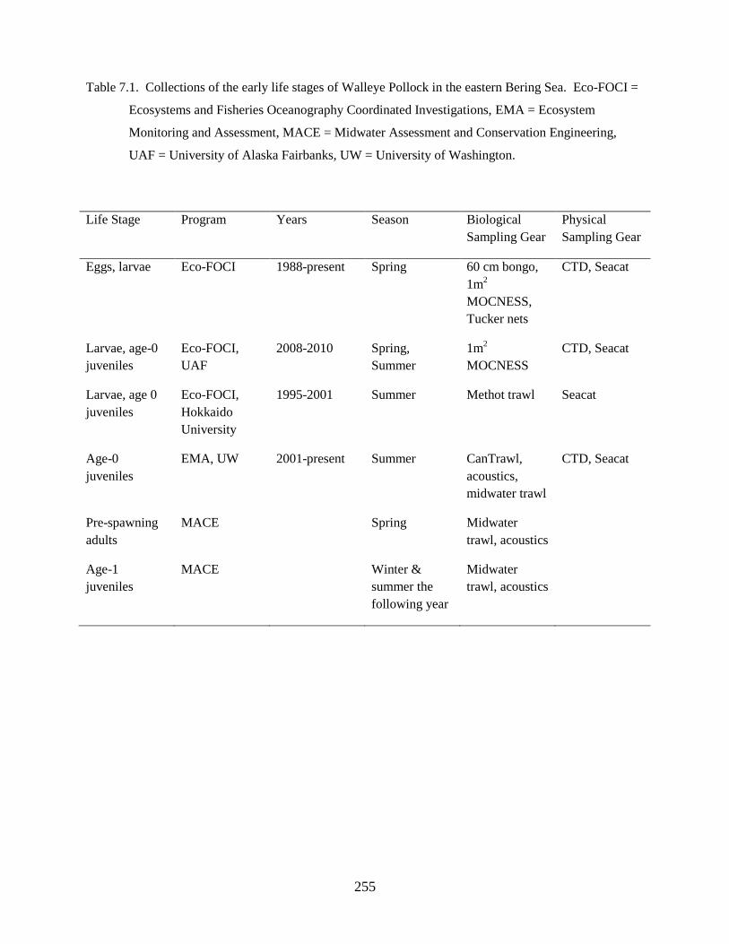
255
Table 7.1. Collections of the early life stages of Walleye Pollock in the eastern Bering Sea. Eco-FOCI =
Ecosystems and Fisheries Oceanography Coordinated Investigations, EMA = Ecosystem
Monitoring and Assessment, MACE = Midwater Assessment and Conservation Engineering,
UAF = University of Alaska Fairbanks, UW = University of Washington.
Life Stage Program Years Season Biological
Sampling Gear
Physical
Sampling Gear
Eggs, larvae Eco-FOCI 1988-present Spring 60 cm bongo,
1m2
MOCNESS,
Tucker nets
CTD, Seacat
Larvae, age-0
juveniles
Eco-FOCI,
UAF
2008-2010 Spring,
Summer
1m2
MOCNESS
CTD, Seacat
Larvae, age 0
juveniles
Eco-FOCI,
Hokkaido
University
1995-2001 Summer Methot trawl Seacat
Age-0
juveniles
EMA, UW 2001-present Summer CanTrawl,
acoustics,
midwater trawl
CTD, Seacat
Pre-spawning
adults
MACE Spring Midwater
trawl, acoustics
Age-1
juveniles
MACE Winter &
summer the
following year
Midwater
trawl, acoustics
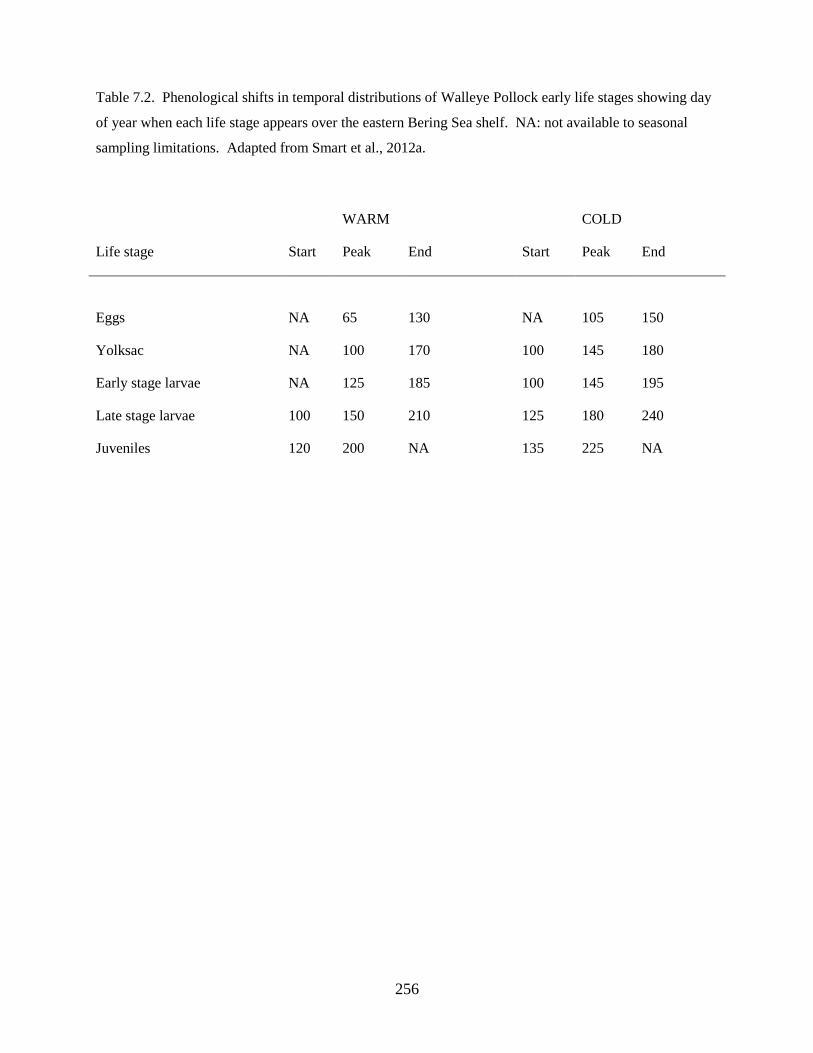
256
Table 7.2. Phenological shifts in temporal distributions of Walleye Pollock early life stages showing day
of year when each life stage appears over the eastern Bering Sea shelf. NA: not available to seasonal
sampling limitations. Adapted from Smart et al., 2012a.
WARM COLD
Life stage Start Peak End Start Peak End
Eggs
NA
65
130
NA
105
150
Yolksac NA 100 170 100 145 180
Early stage larvae NA 125 185 100 145 195
Late stage larvae 100 150 210 125 180 240
Juveniles 120 200 NA 135 225 NA
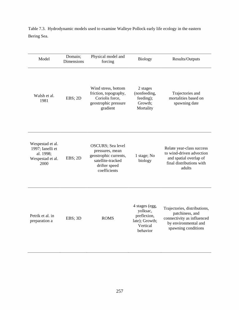
257
Table 7.3. Hydrodynamic models used to examine Walleye Pollock early life ecology in the eastern
Bering Sea.
Model Domain;
Dimensions
Physical model and
forcing Biology Results/Outputs
Walsh et al.
1981 EBS; 2D
Wind stress, bottom
friction, topography,
Coriolis force,
geostrophic pressure
gradient
2 stages
(nonfeeding,
feeding);
Growth;
Mortality
Trajectories and
mortalities based on
spawning date
Wespestad et al.
1997; Ianelli et
al. 1998;
Wespestad et al.
2000
EBS; 2D
OSCURS; Sea level
pressures, mean
geostrophic currents,
satellite-tracked
drifter speed
coefficients
1 stage; No
biology
Relate year-class success
to wind-driven advection
and spatial overlap of
final distributions with
adults
Petrik et al. in
preparation a EBS; 3D ROMS
4 stages (egg,
yolksac,
preflexion,
late); Growth;
Vertical
behavior
Trajectories, distributions,
patchiness, and
connectivity as influenced
by environmental and
spawning conditions
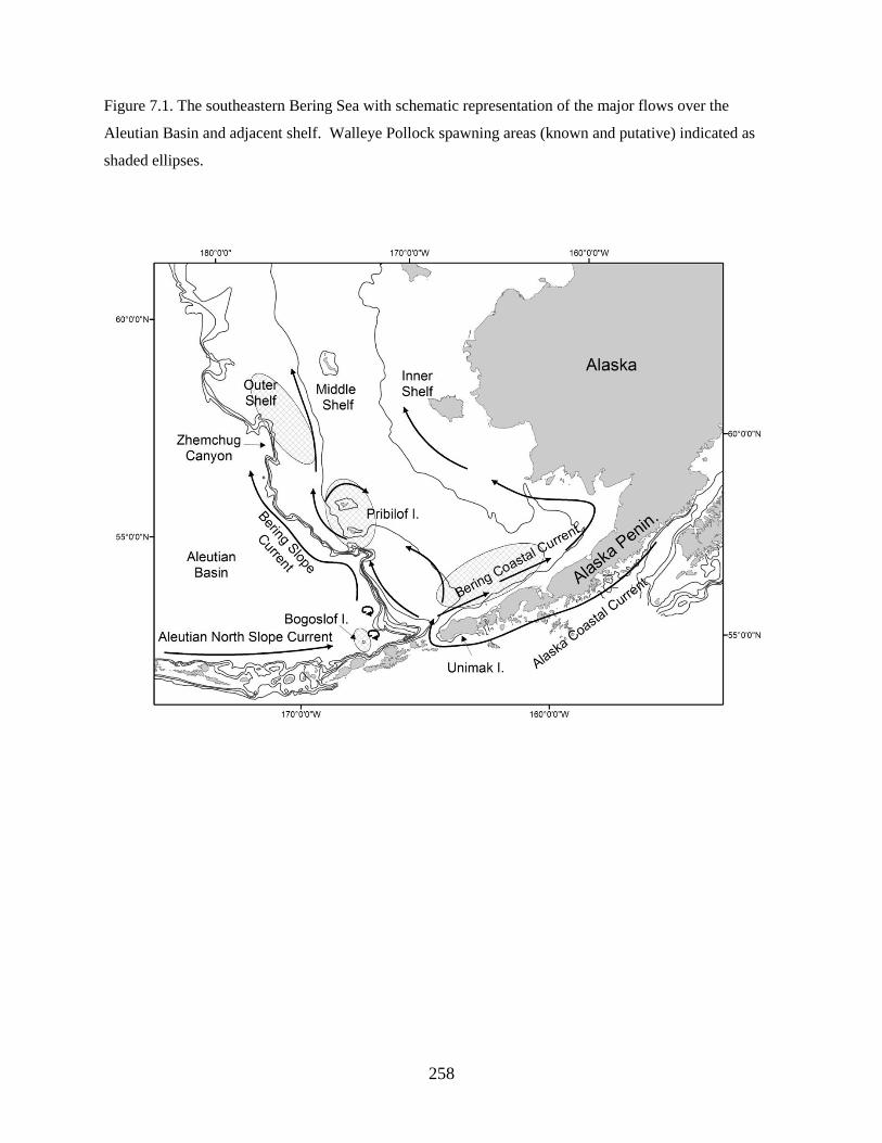
258
Figure 7.1. The southeastern Bering Sea with schematic representation of the major flows over the
Aleutian Basin and adjacent shelf. Walleye Pollock spawning areas (known and putative) indicated as
shaded ellipses.
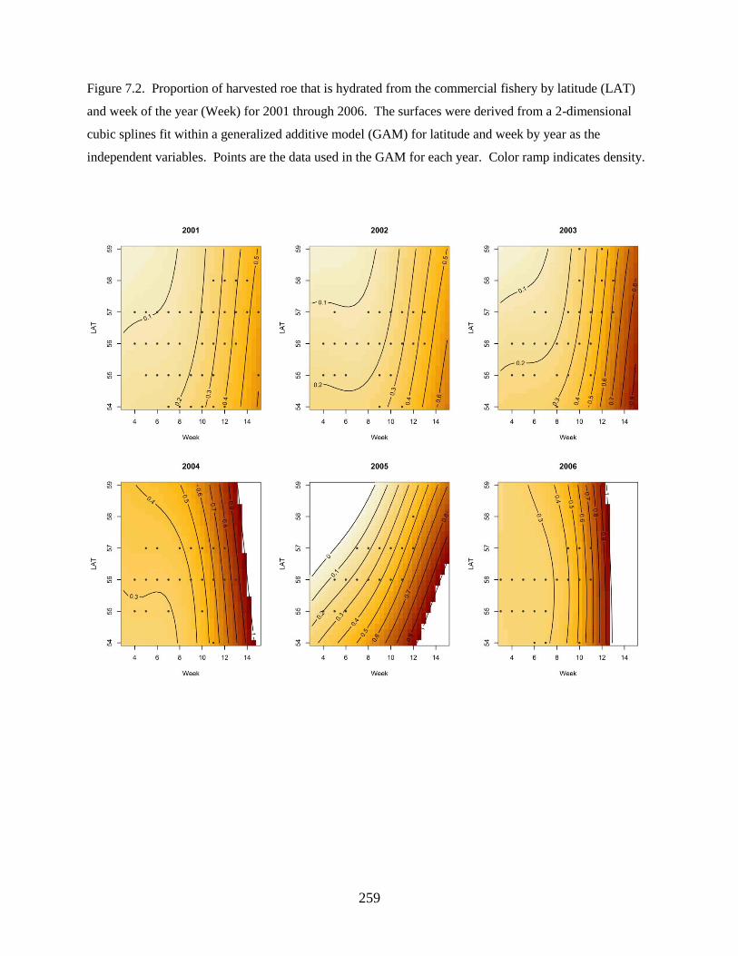
259
Figure 7.2. Proportion of harvested roe that is hydrated from the commercial fishery by latitude (LAT)
and week of the year (Week) for 2001 through 2006. The surfaces were derived from a 2-dimensional
cubic splines fit within a generalized additive model (GAM) for latitude and week by year as the
independent variables. Points are the data used in the GAM for each year. Color ramp indicates density.
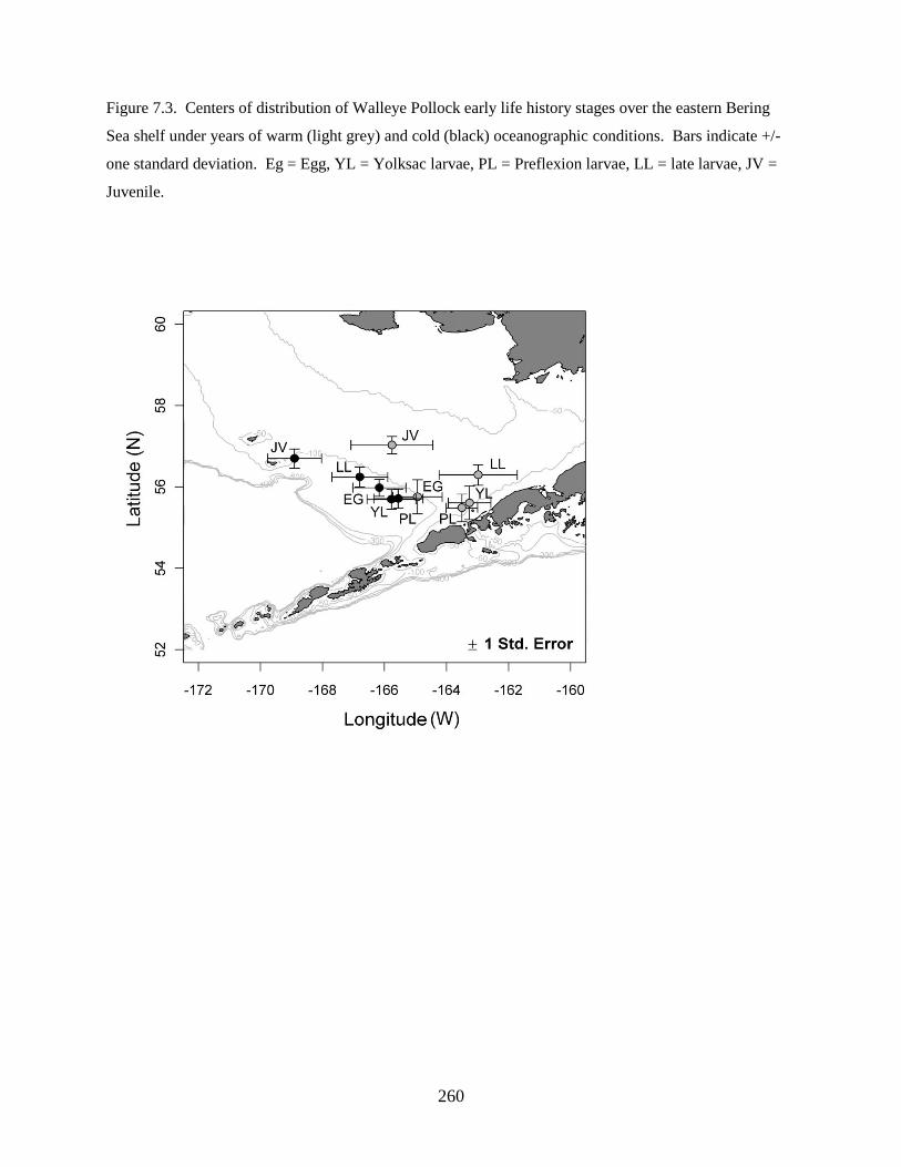
260
Figure 7.3. Centers of distribution of Walleye Pollock early life history stages over the eastern Bering
Sea shelf under years of warm (light grey) and cold (black) oceanographic conditions. Bars indicate +/-
one standard deviation. Eg = Egg, YL = Yolksac larvae, PL = Preflexion larvae, LL = late larvae, JV =
Juvenile.
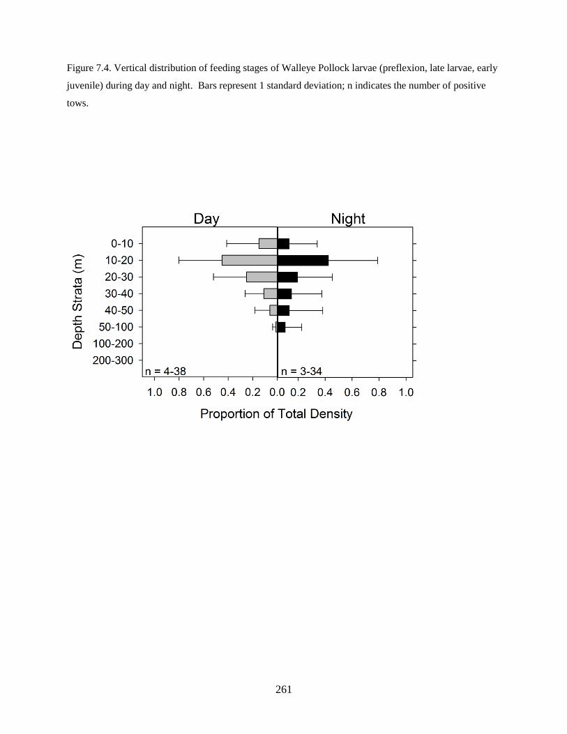
261
Figure 7.4. Vertical distribution of feeding stages of Walleye Pollock larvae (preflexion, late larvae, early
juvenile) during day and night. Bars represent 1 standard deviation; n indicates the number of positive
tows.
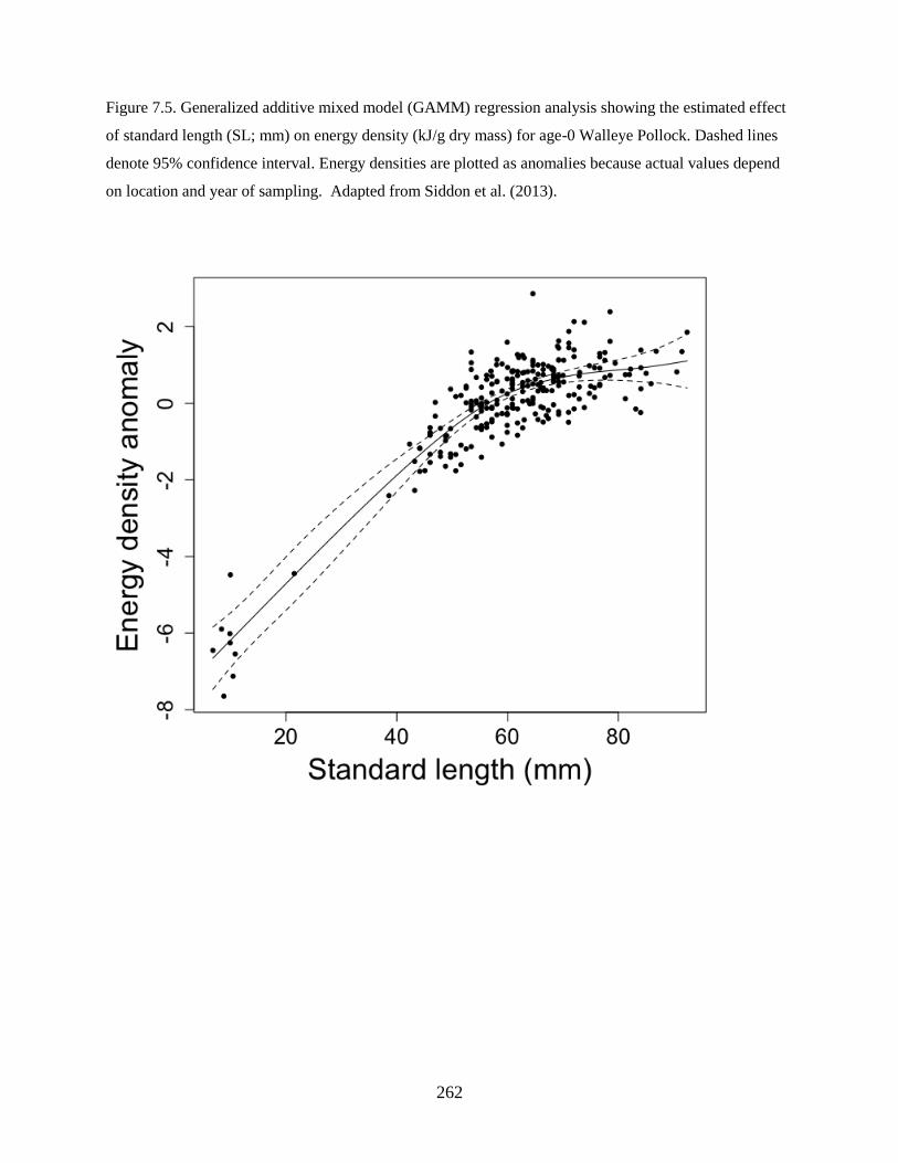
262
Figure 7.5. Generalized additive mixed model (GAMM) regression analysis showing the estimated effect
of standard length (SL; mm) on energy density (kJ/g dry mass) for age-0 Walleye Pollock. Dashed lines
denote 95% confidence interval. Energy densities are plotted as anomalies because actual values depend
on location and year of sampling. Adapted from Siddon et al. (2013).
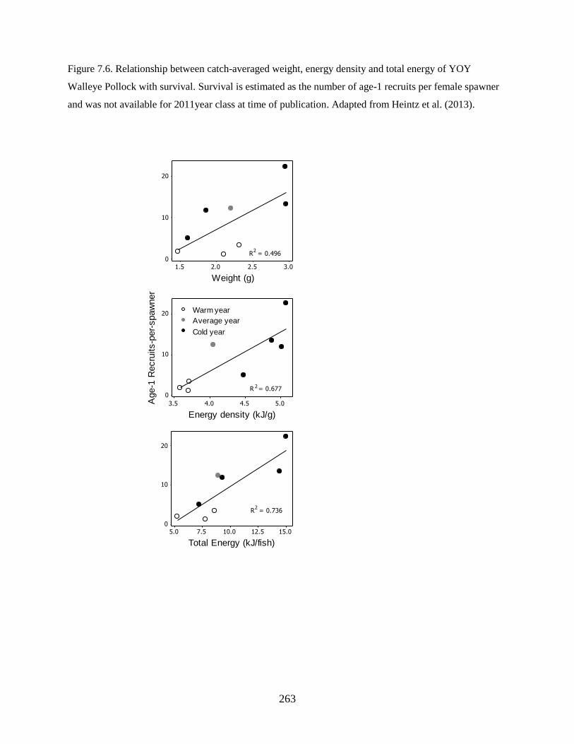
263
Figure 7.6. Relationship between catch-averaged weight, energy density and total energy of YOY
Walleye Pollock with survival. Survival is estimated as the number of age-1 recruits per female spawner
and was not available for 2011year class at time of publication. Adapted from Heintz et al. (2013).
3.02.52.01.5
20
10
0
Weight (g)
5.04.54.03.5
20
10
0
Energy density (kJ/g)
Age-1
Recru
its-p
er-
spaw
ner
Warm year
Average year
Cold year
15.012.510.07.55.0
20
10
0
Total Energy (kJ/fish)
R = 0.4962
R = 0.6772
R = 0.7362
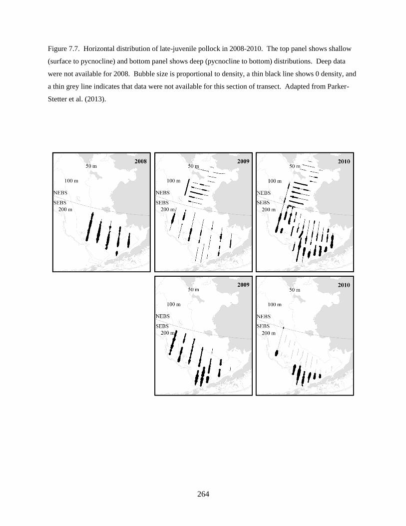
264
Figure 7.7. Horizontal distribution of late-juvenile pollock in 2008-2010. The top panel shows shallow
(surface to pycnocline) and bottom panel shows deep (pycnocline to bottom) distributions. Deep data
were not available for 2008. Bubble size is proportional to density, a thin black line shows 0 density, and
a thin grey line indicates that data were not available for this section of transect. Adapted from Parker-
Stetter et al. (2013).
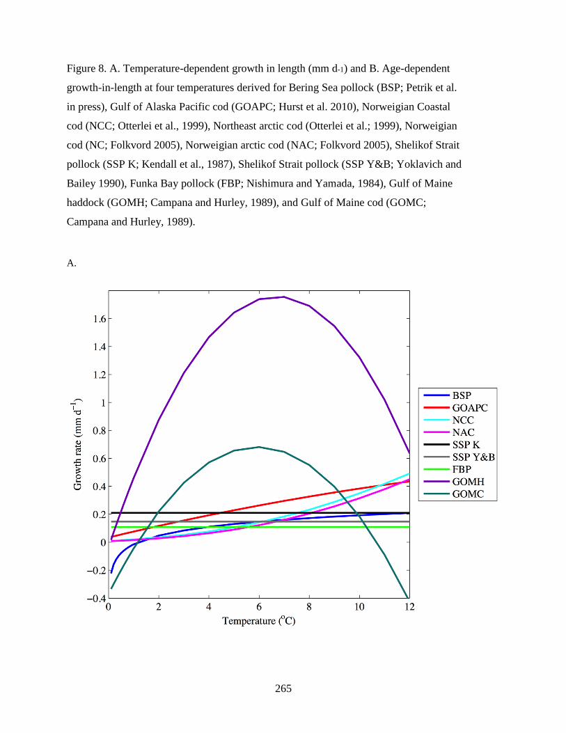
265
Figure 8. A. Temperature-dependent growth in length (mm d-1) and B. Age-dependent
growth-in-length at four temperatures derived for Bering Sea pollock (BSP; Petrik et al.
in press), Gulf of Alaska Pacific cod (GOAPC; Hurst et al. 2010), Norweigian Coastal
cod (NCC; Otterlei et al., 1999), Northeast arctic cod (Otterlei et al.; 1999), Norweigian
cod (NC; Folkvord 2005), Norweigian arctic cod (NAC; Folkvord 2005), Shelikof Strait
pollock (SSP K; Kendall et al., 1987), Shelikof Strait pollock (SSP Y&B; Yoklavich and
Bailey 1990), Funka Bay pollock (FBP; Nishimura and Yamada, 1984), Gulf of Maine
haddock (GOMH; Campana and Hurley, 1989), and Gulf of Maine cod (GOMC;
Campana and Hurley, 1989).
A.
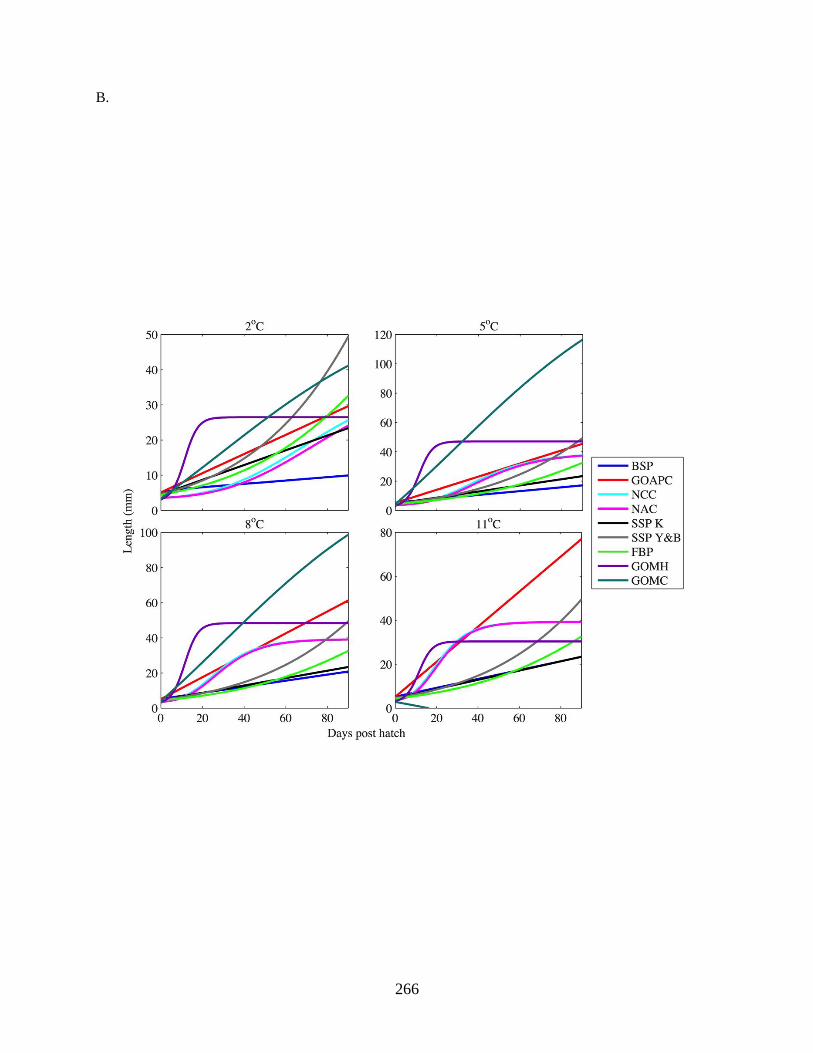
266
B.
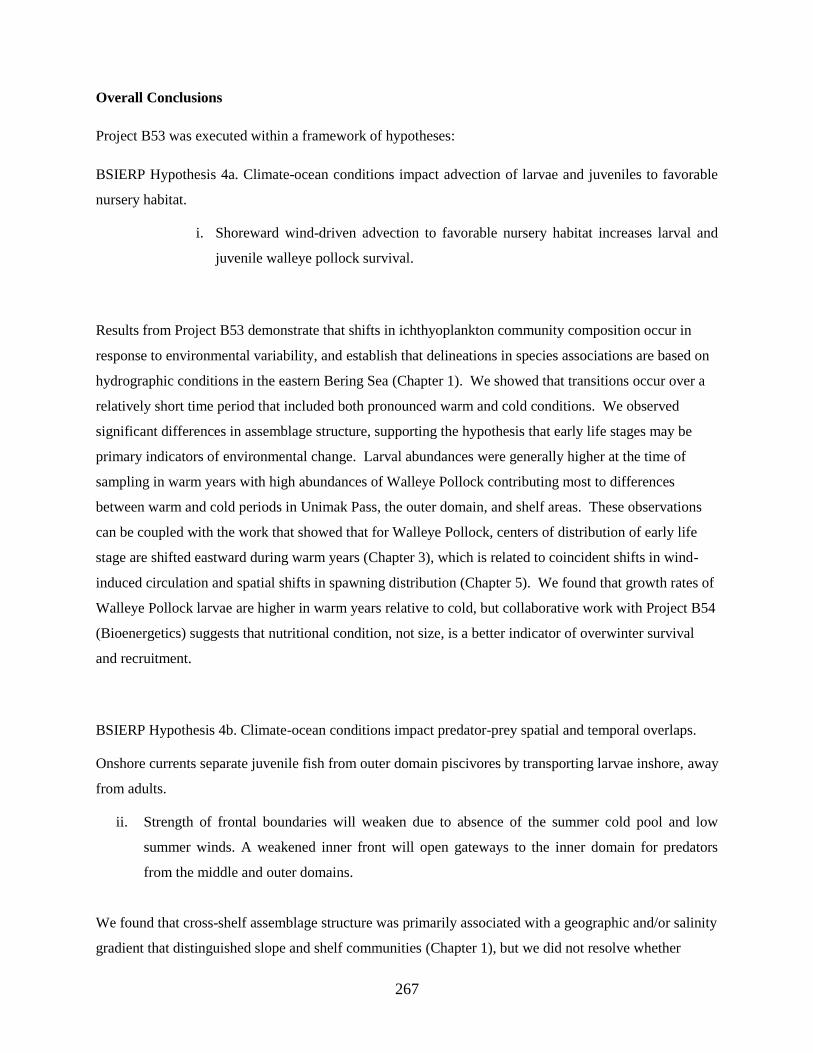
267
Overall Conclusions
Project B53 was executed within a framework of hypotheses:
BSIERP Hypothesis 4a. Climate-ocean conditions impact advection of larvae and juveniles to favorable
nursery habitat.
i. Shoreward wind-driven advection to favorable nursery habitat increases larval and
juvenile walleye pollock survival.
Results from Project B53 demonstrate that shifts in ichthyoplankton community composition occur in
response to environmental variability, and establish that delineations in species associations are based on
hydrographic conditions in the eastern Bering Sea (Chapter 1). We showed that transitions occur over a
relatively short time period that included both pronounced warm and cold conditions. We observed
significant differences in assemblage structure, supporting the hypothesis that early life stages may be
primary indicators of environmental change. Larval abundances were generally higher at the time of
sampling in warm years with high abundances of Walleye Pollock contributing most to differences
between warm and cold periods in Unimak Pass, the outer domain, and shelf areas. These observations
can be coupled with the work that showed that for Walleye Pollock, centers of distribution of early life
stage are shifted eastward during warm years (Chapter 3), which is related to coincident shifts in wind-
induced circulation and spatial shifts in spawning distribution (Chapter 5). We found that growth rates of
Walleye Pollock larvae are higher in warm years relative to cold, but collaborative work with Project B54
(Bioenergetics) suggests that nutritional condition, not size, is a better indicator of overwinter survival
and recruitment.
BSIERP Hypothesis 4b. Climate-ocean conditions impact predator-prey spatial and temporal overlaps.
Onshore currents separate juvenile fish from outer domain piscivores by transporting larvae inshore, away
from adults.
ii. Strength of frontal boundaries will weaken due to absence of the summer cold pool and low
summer winds. A weakened inner front will open gateways to the inner domain for predators
from the middle and outer domains.
We found that cross-shelf assemblage structure was primarily associated with a geographic and/or salinity
gradient that distinguished slope and shelf communities (Chapter 1), but we did not resolve whether
268
strength of the inner front influenced advection to the inner shelf. We did observe however, that the
advection of Alaska Coastal Current waters through Unimak Pass affects the distribution of larval fish on
the EBS shelf. Species entrained in, or advected by, ACC waters within Unimak Pass and the Bering Sea
shelf included Pacific Cod (Gadus macrocephalus) and Northern Rock Sole (Lepidopsetta polyxystra),
with higher overall abundances of these species in warm years. Unfortunately, our sampling design could
not resolve whether these larvae originated in the Gulf of Alaska or were entrained in ACC waters within
Unimak Pass and nearby spawning grounds. The impact of Gulf of Alaska larvae on Bering Sea
populations, and the degree to which the populations are connected, are important ecological (i.e.,
competition, predation) and fisheries management (number of sub-populations) questions. However,
while some studies have demonstrated larval drift from the Gulf of Alaska to the Bering Sea, for most
species the role of advection through Unimak Pass and the resulting connectivity between Gulf of Alaska
and Bering Sea populations is still largely unknown.
BSIERP Hypothesis 4c. Climate-ocean conditions impact the strength of fronts between domains and the
sizes of the domains.
iv. Strength of frontal boundaries will weaken due to absence of the summer cold pool and low
summer winds. Out-migrations of anadromous species will shift away from shore due to the
weakening of the inner front.
v. Strength of the inner front will weaken, allowing expansion of the inner domain, which will
increase the carrying capacity of the inner domain for juveniles.
A coupled ocean-sea ice model, conducted in hindcast mode for the period from 1994-2012, simulated
winds, stratification, ice, currents, and other ocean conditions over nearly two decades, encompassing
both warm and cold years (Chapter 5). The physical model was coupled to an IBM to simulate drift and
transport of Walleye Pollock larvae over the same period. We found that differences in dispersal were
due primarily to differences in spawning locations of adults, rather than to climate-mediated differences
in circulation or to temporal shifts in spawning time. Our results suggest that spatio-temporal variations
in frontal boundaries are not the primary motivator for observed spatial changes in distribution of young
Walleye Pollock.
BSIERP Hypothesis 6. Climate and ocean conditions influencing circulation patterns and domain
boundaries of the eastern Bering Sea shelf will affect the distribution, frequency, and persistence of fronts
and other prey-concentrating features and thus the foraging success of marine birds and mammals.
269
Physical conditions vary interannually over the Bering Sea shelf in response to atmospheric forcing, but
our results suggest that decision-making parameters exhibited by biological organisms responding to
abiotic variation may have a greater role in biotic aggregation (Chapters 3, 4, 5). We found that vertical
distribution of feeding larvae exhibited diel vertical migration, with results suggesting that vertical
distributions and diel migration potentially are driven by prey availability at sufficient light levels for
preflexion larvae to feed and a trade-off between prey access and predation risk for postflexion larvae.
Moreover, model results indicate that horizontal shifts in Walleye Pollock distribution between warm and
cold years were most likely due to spatial shifts in the distribution of spawning adults rather than to
oceanographic changes in frontal structure, stratification, or current direction and velocity alone. We
hypothesize that the spawning area for Walleye Pollock expands and contracts within certain undescribed
geographic boundaries of the broader spawning region, and is dependent upon sea ice presence,
temperature, and population biomass.
The majority of information learned during Project B53 supports a better understanding of the early life
history and ecology of Walleye Pollock. Unfortunately, despite a 20-year history of sampling in the
eastern Bering Sea led by the National Oceanic and Atmospheric Administration, collections of Pacific
Cod and Arrowtooth Flounder larvae are either very few (Pacific Cod) or not to species level (Arrowtooth
Flounder). Instances of catch of Pacific Cod larvae in bongo tows collected from the Bering Sea are
fewer than 300 (http://access.afsc.noaa.gov/ichthyo/index.php), and catches during the BSIERP program
years were less than 20. Records of Arrowtooth Flounder are greater than for Pacific Cod, and catches
were higher during BSIERP years as well, though historical difficulties with taxonomic resolution
between this species and a congeneric, Kamchatka Flounder, Atheresthes evermanni, required that
samples be identified only to the species level. We made great progress in reclassifying historical
samples to the species level using a combination of genetic and morphometric approaches, but ultimately
were not successful at species-specific resolution across all larval size classes. This limited what data
could be put into ecological context and the conclusions that could be derived. Accordingly, data for
Pacific Cod and Arrowtooth Flounder were deemed insufficiently robust to be utilized to the extent we
originally envisioned. As such, we focused on understanding the ecology of Walleye Pollock early life,
and provided information on Arrowtooth Flounder and Pacific Cod where possible.
270
BSIERP and Bering Sea Project Connections
We successfully collaborated with BSIERP projects B54 Seasonal Bioenergetics (Heintz et al.), B59
Surface Trawl Survey Acoustics (Horne, B52 Biophysical Moorings (Stabeno et al.), B90 Surface Trawl
Survey (Farley et al.), and B60 Walleye Pollock and Pacific Cod Distribution (Ciannelli et al.).
Working within an integrated research project such as BSIERP resulted in a far greater understanding of
ichthyoplankton dynamics within the larger framework of the Bering Sea ecosystem. The progression of
BSIERP began with more focused research efforts (i.e., individuals working to meet project-specific
goals), but as projects moved forward, cross-integration became a larger focus. At the onset of the project,
PI meetings felt disparate as projects were just getting “off the ground”. In hindsight, however, this may
be an inevitable part of the progression towards better integration. We felt we had sufficient time to meet
project-specific objectives, while also collaborating with several other efforts to enhance our
understanding of larval ecology across contrasting climate regimes in the EBS.
Seasonal Bioenergetics
On all BSIERP field surveys (2008, 2009, 2010) samples were collected and sent to Juneau, AK for use in
energetic and condition analyses. Samples from age-0 Walleye Pollock and age-0 Arrowtooth Flounder
were provided. Arrowtooth Flounder were conclusively identified at sea prior to shipment from DNA
analyses. Limited samples of Pacific Cod were made available from historical AFSC collections, but
samples were few. Very few Pacific Cod were collected during BSIERP field years. Analyses resulted
in a paper published by a graduate student (Siddon et al. 2013). Collaborations with B53 also included a
co-authored paper on the ecology and bioenergetics of Arrowtooth Flounder (De Forest et al., in press),
and co-authorship on a review paper on pollock ecology during the first year of life in the Bering Sea
(Duffy-Anderson et al., in press). Heintz and Duffy-Anderson also served as external graduate committee
members for graduate student E. Siddon (PhD, UAF). Work from the Siddon dissertation applied to both
projects. Other work included a collaborative paper on condition and recruitment of age-0 pollock
(Heintz et al. 2013)
Surface Trawl Survey Acoustics
We collaborated with project B59 by jointly advising postdoctoral researcher (T. Smart). Dr. Smart
worked with J. Horne and S. Parker-Stetter to examine factors affecting abundance of pollock in the EBS
(Smart et al. 2012 a, b) and vertical distribution of pollock in the EBS (Smart et al. 2013). Collaboration
also included co-authorship on a review paper on pollock ecology during the first year of life in the
Bering Sea (Duffy-Anderson et al. in press).
Biophysical Moorings
271
Collaborations with this project included joint ship time to recover/deploy BSIERP moorings collect
zooplankton samples around moorings along the 70 m isobath. Data from a portion of the joint sampling
was used in Smart et al. 2011. Collaborations also included discussion of implications of results from
Smart et al. 2011 and Smart et al. 2012a. Other collaborative papers include Stabeno et al. 2012, Stabeno
et al. in press.
Surface Trawl Survey
All ichthyoplankton from surface trawl surveys (BASIS) were sorted and identified by the FOCI Program
as matching contribution (Ann Matarese lead). All data were provided to BSIERP research. We also
collaborated with this project via sample sharing (3 BSIERP target fish species, zooplankton analyses and
information), and through the efforts of UAF graduate student E. Siddon and postdoctoral researcher T.
Smart. Collaborations resulted in two co-authored publications (Smart et al. 2012a) and Duffy-Anderson
et al. (in press). Other collaborations include Hunt et al. 2011 and Sigler et al. 2012.
Walleye Pollock and Pacific Cod Distribution
We collaborated with this project by providing historical data from AFSC ichthyoplankton surveys to
postdoctoral researcher N. Bacheler for use in data analyses and interpretation. Data sharing resulted in
three publications, Bacheler et al. 2009, Bachelor et al. 2010 (co-authored with J. Duffy-Anderson), and
Bacheler et al. (2012). These publications helped elucidate spawning areas of Walleye Pollock in the
Bering Sea, effects of water temperature on pollock spawning phenology, and landscape ecology and
density-dependent effects of spawning biomass on egg density. We also collaborated on a paper to
examine how variations in major currents (Bering Slope Current, cross-shelf currents) affect recruitment
of Walleye Pollock, Pacific Cod, Arrowtooth Flounder (Vestfals et al. in press). In addition, L. Ciannelli
trained postdoctoral associate T. Smart in spatial statistics for use in data analyses.
272
Management Implications
Predictions of continued warming trends in the Bering Sea heighten the need for mechanistic
understanding of factors that contribute to spatial and temporal shifts in Walleye Pollock biomass and to
variations in Walleye Pollock recruitment. It has long been recognized that population variability of
fecund marine species like Walleye Pollock is linked to factors influencing growth and survivorship of
early life history stages. Results from this project contribute to the growing body of knowledge of factors
influencing Walleye Pollock distribution, growth, abundance, survivorship, and recruitment.
Our work is useful to stock assessment and research managers and stakeholders as it identifies
critical areas of young Walleye Pollock production, which appear to be spatially and temporally variable
and dependent on climate conditions. This has important implications for management of the Walleye
Pollock roe fishery, which targets pre-spawning adults for commercial harvest. In addition, these dynamic
areas could be considered Essential Fish Habitat (EFH) for Walleye Pollock during spawning periods.
Next, we demonstrate that oceanographic conditions, in particular, temperature and zooplankton
prey availability, have pronounced effects not only on distribution of young fish but also on Walleye
Pollock rates of growth and mortality in the months prior to onset of the first winter. There is increasing
awareness that the quality of prey available to juvenile Walleye Pollock has an impact on recruitment
success. Results from our study, combined with those from B54 Seasonal Bioenergetics (Heintz et al.)
demonstrate mechanisms leading to differences in recruitment success under varying climate conditions.
Such biological responses to broad-scale climate changes can be incorporated into the stock assessment to
better predict recruitment success under future climate scenarios.
Finally, our work also points to the likelihood of thermally-mediated spatial expansions and
contractions of spawning areas, which is of significant interest to managers since contractions in spatial
spawning extent can be indicative of overall declines in population biomass. Additionally, changes in
spatial extent may result in changes in predator-prey dynamics; such information could be used in
Integrated Ecosystem Assessments (IEA; www.noaa.gov/iea).
We note that continued monitoring of Walleye Pollock populations in the eastern Bering Sea is
central to honing predictive capability. Long-term programs to monitor and evaluate interannual spatial
and temporal spawning variations, diet and nutritional condition of larvae and juveniles, and stage-
specific shifts in centers of distribution is central to validating the above observations and providing
stakeholders useful quantitative tools to successfully manage the fishery.
273
Publications (*primary and collaborative with other BSIERP projects)
*De Forest, L., Duffy-Anderson, J.T., Heintz, R., Matarese, A.M., Siddon, E., Smart, T. and Spies, I. In
press. Ecology and taxonomy of the early life stages of arrowtooth (Atheresthes stomias) and
Kamchatka (Atheresthes evermanni) flounder in the eastern Bering Sea. Deep Sea Research II:
Topical Studies in Oceanography. http://dx.doi.org/10.1016/j.dsr2.2014.05.005
*Duffy-Anderson, J.T., Barbeaux, S., Farley, E., Heintz, R., Horner, J., Parker-Stetter, S., Petrik, C.,
Siddon, E.C., and Smart, T.I. In review. An ecological synthesis of the first year of life of
Walleye Pollock (Gadus chalcogrammus) in the eastern Bering Sea. Deep Sea Research II:
Topical Studies in Oceanography.
Heintz, R.A., Siddon, E.C., Farley Jr, E.V., Napp, J.M. 2013. Correlation between recruitment and fall
condition of age-0 pollock (Theragra chalcogramma) from the eastern Bering Sea under varying
climate conditions. Deep Sea Research II: Topical Studies in Oceanography. 94:150-156.
Hunt, G.L., Coyle, K.O., Eisner, L.B., Farley, E.V., Heintz, R., Mueter, F.J., Napp, J.M., Overland, J.E.,
Ressler, P.H., Salo, S., Stabeno, P.J. 2011. Climate impacts on eastern Bering Sea foodwebs: a
synthesis of new data and an assessment of the Oscillating Control Hypothesis. ICES Journal of
Marine Science. 68: 1230-1243.
*Petrik, C., Duffy-Anderson, J.T., Mueter, F.J., Hedstrom, K., and Curchitser, E. In press. Modeling the
effect of climate variations on the transport and distribution of Walleye Pollock early life stages
in the eastern Bering Sea. Progress in Oceanography.
http://www.sciencedirect.com/science/article/pii/S0079661114001128
*Siddon, E.C., Duffy-Anderson, J.T., and Mueter, F. 2011. Community-level response of
ichthyoplankton to environmental variability in the eastern Bering Sea. Marine Ecology Progress
Series. 426: 225-239.
Sigler, M.F., Harvey, H.R., Ashjian, C.J., Lomas, M.W., Napp, J.M., Stabeno, P.J., Van Pelt, T. 2012.
How does climate change affect the Bering Sea Ecosystem? EOS. 91: 457-468.
*Smart, T., Duffy-Anderson, J.T., Horne, J. 2012a. Alternating climate states influence Walleye Pollock
life stages in the southeastern Bering Sea. Marine Ecology Progress Series. 455: 257-267.
*Smart, T., Duffy-Anderson, J.T., Horne, J., Farley, E., Wilson, C., and Napp, J. 2012b. Influence of
environment on Walleye Pollock eggs, larvae, and juveniles in the Southeastern Bering Sea.
Deep Sea Res. II: Topical Studies in Oceanography. 65-70: 196-207.
274
*Smart, T., Duffy-Anderson, J.T., and Siddon, E. 2013. Vertical distribution of early life stages of
walleye Pollock and implications for transport and connectivity. Deep Sea Research II: Topical
Studies in Oceanography. 94: 201-201.
Stabeno P.J., Farley E.V. Jr, Kachel N.B., Moore S., Mordy C.W., Napp J.M., Overland J.E., Pinchuk
A.I., Sigler M.F. 2012. A comparison of the physics of the northern and southern shelves of the
eastern Bering Sea and some implications for the ecosystem. Deep Sea Research II: Topical
Studies in Oceanography. 65-70: 14-30.
Stabeno, P.J., Kachel, N.B., Moore, S., Napp, J.M., Sigler, M.F., Yamaguchi, A., Zerbini, A.N. In press.
Comparison of warm and cold years on the southeastern Bering Sea shelf and some implications
for the ecosystem. Deep Sea Research II: Topical Studies in Oceanography. 65-70: 31-45.
Stabeno P.J., Napp J.M., Mordy C., Whitledge T. 2010. Factors influencing physical structure and lower
trophic levels of the eastern Bering Sea shelf in 2005: Sea ice, tides and winds. Progress in
Oceanography. 85: 180-196.
Vestfals, C., Ciannelli, L., Duffy-Anderson, J.T., and Ladd, C. In press. Effects of seasonal and
interannual variability of along-shelf and cross-shelf transport on groundfish recruitment in the
eastern Bering Sea. Deep Sea Research II: Topical Studies in Oceanography.
275
Poster and Oral Presentations (*Indicates award winner)
Bacheler, N., Ciannelli, L., Duffy-Anderson, J.T. and Bailey, K. Distribution of Walleye Pollock,
Atheresthes. spp., and Pacific Cod early life history stages in the Bering Sea. 2008. Poster, North
Pacific Research Board Annual Meeting. Anchorage, AK. October.
De Forest, L., Duffy-Anderson, J., Heintz, R., Matarese, A., Siddon, E., Smart, T., and Spies, I. 2011.
Current knowledge of the early life history of arrowtooth flounder (Atheresthes stomias) in the
eastern Bering Sea: with comments on Kamchatka flounder (A. evermanni). Gilbert
Ichthyological Society, Seabeck, WA. October.
De Forest, L., Smart, T., Duffy-Anderson, J., Matarese, A., Heintz, R., Siddon, E., Spies, I., and Cooper,
D. 2011. Current knowledge of the early life history of arrowtooth flounder (Atheresthes stomias)
in the eastern Bering Sea: with comments on Kamchatka flounder (A. evermanni). Poster,
International Flatfish Symposium, Ijmuiden, Netherlands. November.
De Forest, L., Duffy-Anderson, J.T., Heintz, R., Matarese, A., Siddon, E., Smart, T., and Spies, I. 2013.
Current knowledge on the ecology and taxonomy of the early life stages of arrowtooth
(Atheresthes stomias) and Kamchatka flounder (A. evermanni) in the eastern Bering Sea. (Poster)
Alaska Marine Science Symposium Anchorage, AK. January.
De Forest, L., Duffy-Anderson, J., Heintz, R., Matarese, A., Siddon, E., Smart, T., and Spies, I. 2013.
Ecology and taxonomy of the early life stages of arrowtooth flounder (Atheresthes stomias) and
Kamchatka flounder (A. evermanni) in the eastern Bering Sea. Larval Fish Conference, Miami,
FL. June.
Duffy-Anderson, J.T. 2011. Ichthyoplankton dynamics and seasonal bioenergetics in the southeast
Bering Sea. NPRB BSIERP PI Meeting, Anchorage, AK. March.
Duffy-Anderson, J.T., Hillgruber, N., Napp, J., Matarese, A., Eisner, L., and Heintz, R. 2009.
Ichthyoplankton dynamics and seasonal bioenergetics in the eastern Bering Sea. North Pacific
Research Board Annual Meeting. Girdwood, AK. October.
Duffy-Anderson, J.T., Siddon, E., Smart, T., and Hillgruber, N. 2009. Vertical distribution of larval
Walleye Pollock, Pacific Cod, and Arrowtooth Flounder in the eastern Bering Sea. North Pacific
Research Board Annual Meeting. Girdwood, AK. November.
Duffy-Anderson, J.T., Smart, T.I., Siddon, E., Mueter, F., Matarese, A., Eisner, L., Napp, J., and Heintz,
R. 2011. Ichthyoplankton and seasonal bioenergetics. BSIERP PI Meeting, Anchorage, AK.
January.
276
Matarese, A., De Forest, L., Duffy-Anderson, J., Smart, T., and Spies, I. 2013. Identification and
distribution of the early life stages of arrowtooth (Atheresthes stomias) and Kamchatka flounder
(A. evermanni) in the eastern Bering Sea. (Poster) Larval Fish Conference, Miami, FL. June.
Napp, J.M., Eisner, L.B., Farley, E.W., Stabeno, P.J., Hunt, Jr., G.L. 2010. Recent changes in
zooplankton abundance and biomass in the eastern Bering Sea, Alaska Marine Science
Symposium, Anchorage, AK, January.
Napp, J.M., Sigler, M.F., and Stabeno, P.J. Understanding ecosystem processes in the Bering Sea. 2010.
NOAA Headquarters Lunch Seminar, Silver Spring, MD, March.
Hillgruber, N., Duffy-Anderson, J.T., Eisner, L., Heintz, R., Matarese, A., Napp, J., and Siddon, E. 2008.
Distribution, transport, and condition of early life stages of Walleye Pollock, Pacific Cod, and
Arrowtooth Flounder in the eastern Bering Sea under the auspice of changing climatic conditions.
Contributed poster. Larval Fish Conference. Kiel, Germany. August.
Petrik, C.M., Duffy-Anderson, J.T., Mueter, F., Hedstrom, K., Danielson, S., Curchitser, E., and
Barbeaux, S. 2013. Modeling climate effects on the dispersal and distribution of pollock early
life stages in the eastern Bering Sea. ICES Annual Science Conference. Reykjavik, Iceland.
September.
*Petrik, C.M., Duffy-Anderson, J.T., Mueter, F., Hedstrom, K., Danielson, S., Curchitser, E., and
Barbeaux, S. 2013. Modeling climate effects on the dispersal and distribution of pollock early
life stages in the eastern Bering Sea. PICES Annual Science Conference. Nanaimo, British
Columbia. October. *Best Paper, Physical Oceanography section
*Siddon, E., Duffy-Anderson, J.T., and Mueter, F. 2010. Community-level response of ichthyoplankton
to environmental variability in the eastern Bering Sea. Western Groundfish Conference. April.
Juneau, AK.*Best Student Paper Award
Smart, T.I. and Duffy-Anderson, J.T. The Use of Generalized Additive Models to Investigate Alternating
Environmental States and the Early Life Stages of Walleye Pollock in the Eastern Bering Sea.
2010. Quantitative Seminar Series, School of Aquatic and Fishery Sciences, UW, January.
Smart, T.I. and Duffy-Anderson, J.T. Alternating Environmental States and the Early Life Stages of
Walleye Pollock in the Eastern Bering Sea. 2010. EcoFOCI Seminar Series, NOAA/AFSC,
December.
277
Smart, T.I., Siddon, E., Duffy-Anderson, J.T., and Hillgruber, N. 2009. Vertical distribution of larval
Walleye Pollock (Theragra chalcogramma), Pacific Cod (Gadus macrocephalus), and
Atheresthes spp. in the eastern Bering Sea (poster). BEST-BSIERP Principal Investigators
Meeting, October.
Smart, T., Duffy-Anderson, J.T., and Horne, J. 2011. Alternating climate states influence Walleye
Pollock early life stages in the southeastern Bering Sea. PICES/ESASS Symposium. May.
Smart, T., Duffy-Anderson, J.T., Horne, J., and Farley, E. 2011. Alternating climate states influence
Walleye Pollock early life stages in the southeastern Bering Sea. Alaska Marine Science
Symposium. January.
Smart, T.I., Duffy-Anderson, J.T., Horne, J., Farley, E., Stabeno, P. 2010. Alternating climate states and
the effects on vital rates of Walleye Pollock early life stages in the Bering Sea. Oral presentation,
Larval Biology Symposium, Wellington, NZ. August.
Smart, T., Siddon, E.C., Duffy-Anderson, J.T., and Hillgruber, N. 2010. Vertical distribution of two
common larval gadids, Walleye Pollock (Theragra chalcogramma) and Pacific Cod (Gadus
macrocephalus), in the eastern Bering Sea and their relationships with climate variables. Ocean
Sciences Meeting. Portland, OR. February.
*Siddon, E., Duffy-Anderson, J.T., Mueter, F., and Hillgruber, N. 2010. Interannual variability in cross-
shelf assemblage structure of ichthyoplankton in the eastern Bering Sea. Alaska Marine Science
Symposium, January. Anchorage, AK. *Best Student Paper Award
Siddon, E.C. Mueter, F.J., Heintz, R., and Duffy-Anderson, J.T. 2012. Shifts in community structure
reflect species-specific responses to climate variability in sub-arctic seas. PICES Early Career
Scientist Conference. Mallorca, Spain. April.
Smart, T., Siddon, E., Duffy-Anderson, J.T., and Hillgruber, N. 2009. Vertical distribution of larval
Walleye Pollock, Pacific Cod, and Arrowtooth Flounder in the eastern Bering Sea. North Pacific
Research Board Annual Meeting. Girdwood, AK. October.
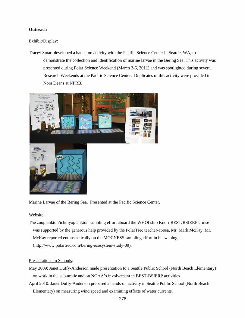
278
Outreach
Exhibit/Display:
Tracey Smart developed a hands-on activity with the Pacific Science Center in Seattle, WA, to
demonstrate the collection and identification of marine larvae in the Bering Sea. This activity was
presented during Polar Science Weekend (March 3-6, 2011) and was spotlighted during several
Research Weekends at the Pacific Science Center. Duplicates of this activity were provided to
Nora Deans at NPRB.
Marine Larvae of the Bering Sea. Presented at the Pacific Science Center.
Website:
The zooplankton/ichthyoplankton sampling effort aboard the WHOI ship Knorr BEST/BSIERP cruise
was supported by the generous help provided by the PolarTrec teacher-at-sea, Mr. Mark McKay. Mr.
McKay reported enthusiastically on the MOCNESS sampling effort in his weblog
(http://www.polartrec.com/bering-ecosystem-study-09).
Presentations in Schools:
May 2009: Janet Duffy-Anderson made presentation to a Seattle Public School (North Beach Elementary)
on work in the sub-arctic and on NOAA’s involvement in BEST-BSIERP activities
April 2010: Janet Duffy-Anderson prepared a hands-on activity in Seattle Public School (North Beach
Elementary) on measuring wind speed and examining effects of water currents.
279
March 2012: Janet Duffy-Anderson presented a marine plankton display as part of Science Day in Seattle
Public Schools. The presentation included several data examples from this project.
Community Meeting:
Franz Mueter presented a public seminar in Nome, Alaska, on May 29, 2012, on the spatial dynamics of
fishes in the Bering Sea with a special focus on the northern Bering Sea. The presentation
included examples of the distribution of early life stages from this project.
280
Acknowledgements
Funding for this project was provided by, the North Pacific Research Board’s Bering Sea Integrated
Ecosystem Research Program, the National Science Foundation’s Bering Ecosystem Study program,
NOAA Fisheries Alaska Fisheries Science Center’s Ecosystem and Fisheries Oceanography Coordinated
Investigations program, the University of Alaska, the University of Washington’s School of Aquatic and
Fishery Sciences, and Oregon State University’s College of Earth, Ocean, and Atmospheric Sciences.