NORTH DAKOTA GAME AND FISH DEPARTMENT

Final Report

Grassland Bird Response to Decreases in Grazing Pressure

Project T-31-R

April 1, 2011 – March 31, 2014

Terry Steinwand Director

Submitted by Greg Link

Chief, Conservation and Communications Division

June 2014

1

Final Report March 2014 Prepared by: Marissa Ahlering Project Title: Grassland Bird Response to Decreases in Grazing Pressure Species of Conservation Priority: Level 1: Willet, Upland Sandpiper, Marbled Godwit, Grasshopper Sparrow, Nelson’s Sparrow; Level 2: Sedge Wren, Dickcissel, Bobolink Contact Information: Principal Investigator: Dr. Marissa Ahlering

Title: Prairie Ecologist Organization: The Nature Conservancy

Address: 938 Lincoln, Vermillion, SD 57069 Phone: 605-658-0209 Email: mahlering@tnc.org Activity Period: April 1, 2011 – March 31, 2014 Location: The project took place in the Sheyenne River Delta area in the counties of Ransom and Richland. The research and monitoring was carried out on The Nature Conservancy (TNC)-owned Brown Ranch and the U. S. Forest Service (USFS)-owned Sheyenne National Grasslands. Overview of Project The North Dakota Comprehensive Wildlife Conservation Strategy (Hagen et al. 2005) and The Nature Conservancy (Sheyenne River Conservation Action Plan) both identify improper grazing practices as a threat to the tallgrass prairie in the Sheyenne River Delta. The goal of this project was to provide information about how to reduce the threat of improper grazing practices by examining the impacts of reduced grazing pressure on TNC properties in the landscape. Reduced grazing pressure should provide more habitat heterogeneity in the overall landscape, and increase the availability of high quality prairie for grassland breeding birds, such as Upland Sandpipers, Grasshopper Sparrows, Nelson’s Sparrows, Sedge Wren, Dickcissel, and Bobolink. The goal was to gain information about grassland bird response to grazing that could leverage changes in grazing practices on other agency and private lands. Objectives:

1. Conduct grassland bird surveys across TNC’s ~2,000 acres of grassland in the Sheyenne River Delta, with replication across areas with traditional and recently reduced grazing pressure.

2. Determine whether a reduction in grazing pressure increases the abundance of grassland breeding birds. 3. Determine whether a reduction in grazing pressure changes the composition of the grassland breeding bird

community. 4. Conduct vegetation sampling using belt transects, structural measurements and biomass clippings. 5. Evaluate the change in range condition (biomass productivity and invasive species) after grazing pressure is

reduced. Overall Summary Bird community richness on The Nature Conservancy pastures where grazing intensity had been reduced was similar to the USFS pastures where grazing intensity was consistently higher. However, some interesting trends in abundance for the four focal species were apparent. Grasshopper Sparrows, Upland Sandpipers and Bobolinks were all positively related to grazing intensity, with grazing intensity being the strongest predictor of abundance for the Grasshopper Sparrow. Upland Sandpipers were most strongly predicted by the occurrence of a recent burn, with lower abundances in those areas. Bobolink abundance was best predicted by vegetation characteristics and ecological site descriptions, and Marbled Godwit abundance was best predicted by burning and vegetation characteristics. The Nature Conservancy pastures were more heavily dominated by native vegetation but had higher

2

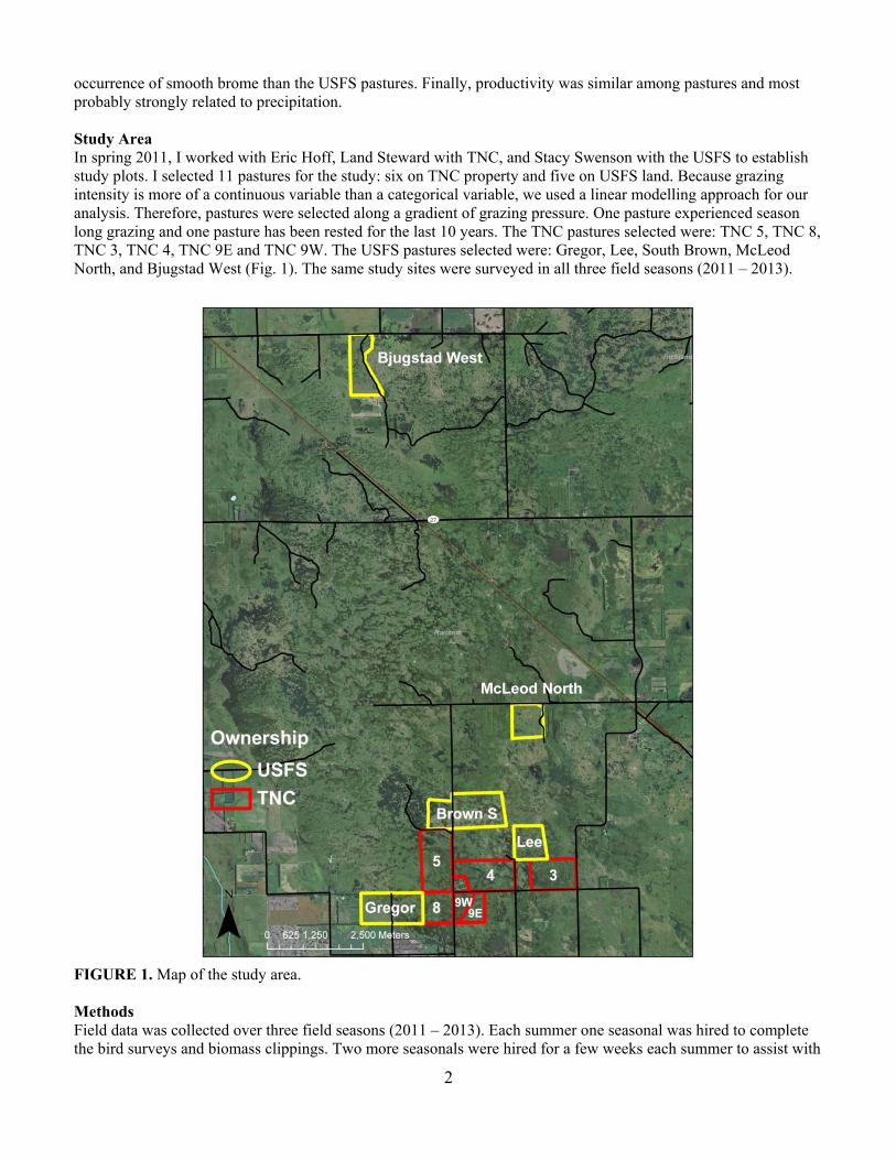
occurrence of smooth brome than the USFS pastures. Finally, productivity was similar among pastures and most probably strongly related to precipitation. Study Area In spring 2011, I worked with Eric Hoff, Land Steward with TNC, and Stacy Swenson with the USFS to establish study plots. I selected 11 pastures for the study: six on TNC property and five on USFS land. Because grazing intensity is more of a continuous variable than a categorical variable, we used a linear modelling approach for our analysis. Therefore, pastures were selected along a gradient of grazing pressure. One pasture experienced season long grazing and one pasture has been rested for the last 10 years. The TNC pastures selected were: TNC 5, TNC 8, TNC 3, TNC 4, TNC 9E and TNC 9W. The USFS pastures selected were: Gregor, Lee, South Brown, McLeod North, and Bjugstad West (Fig. 1). The same study sites were surveyed in all three field seasons (2011 – 2013).

FIGURE 1. Map of the study area. Methods Field data was collected over three field seasons (2011 – 2013). Each summer one seasonal was hired to complete the bird surveys and biomass clippings. Two more seasonals were hired for a few weeks each summer to assist with

3

the vegetation surveys. At the end of each season, the exact dates and stocking densities for each pasture were collected from TNC and the USFS along with the records for any prescribed fires or wildfires on the sites. Point Counts We surveyed a total of 61 randomly located point counts across all 11 study pastures. Point counts were 5 min. in length, started a half an hour before sunrise, stopped by 10:00 am in the morning and were done with good visibility and low wind conditions. At each point, we used laser range finders to estimate the distance to four focal species: Bobolinks, Grasshopper Sparrows, Upland Sandpipers and Marbled Godwits. We recorded presence/absence of all other species at the points. All points were visited 5 times throughout the summer between mid-May and the end of July. The same points were surveyed in all three field seasons. The observer was the same throughout each individual field season but differed among all three years. Vegetation Transects We used a modified belt transect to measure the vegetation in all the pastures (Grassland Monitoring Team Protocol v.7). We established one transect for every 10 acres in each pasture. Each transect was 25 m long and composed of 50 subplots. A vegetation community type was assigned to each subplot, and litter depth and vegetation height were measured at 5 m intervals along the transect. One Robel pole reading was taken at the center of each transect (Robel et al. 1970) to get a Visual Obstruction Reading (VOR), and a list of invasive and native indicator species was used as a checklist for each transect. These transects gave us an indication of vegetation structure and composition over the course of the study. We established a total of 210 transects across all 11 pastures. The same transects were surveyed in all three field seasons. Biomass Clipping We established 3 enclosures in each pasture to collect biomass clippings at the end of the field season. Clipping was done from the center of each enclosure during the second week in August. The enclosures worked well and were moved to new locations in each pasture in subsequent field seasons. The clippings were frozen until they were dried and weighed. Weather Data Precipitation varied quite a bit among the three field seasons. We obtained the precipitation data from the weather station in McLeod, ND. We obtained the annual precipitation for each field season from the previous year (e.g., for 2011 field season we used precipitation from the previous May 2010 – April 2011). The precipitation from the previous growing season and snow from the previous winter is what will impact the vegetation productivity and structure for a given field season. Management Data We collected the burning and grazing information for all 11 pastures each year. To standardize the grazing information, we used a grazing intensity measure in our models calculated as the number of animal months per acre. We used animal month instead of animal unit months because we did not have the information to correct for weight of the animals. Because birds have generally already arrived before animals are turned out into the pastures in mid to late May, we used the grazing intensity from the previous year to relate to bird abundance. The intensity of grazing the previous year is what would most strongly influence the vegetation and habitat that the birds have to select when they arrive the following spring. Both prescribed fire and wildfire occurred on our study sites during the course of the study. Burning can strongly influence the vegetation and habitat of the grasslands the year of a fire (Grant et al. 2010). We used a status of burned or not burned as a variable in our model, and a site-year combination was given a status of burned if it was burned at any time during the previous dormant season. Statistical Analysis We used the package unmarked in program R (Team 2014) to evaluate the impact of grazing, burning, precipitation, year, and vegetation variables on abundance of our four focal species: Grasshopper Sparrow, Upland

4

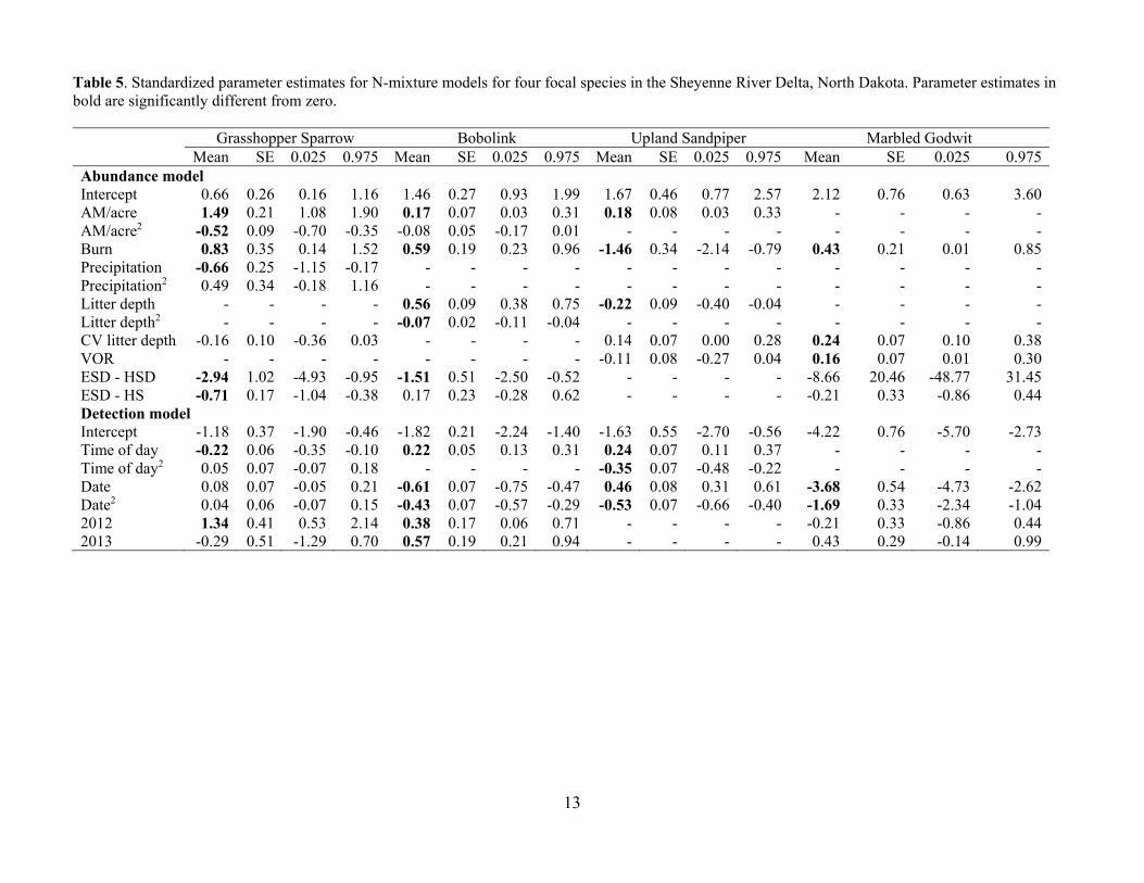
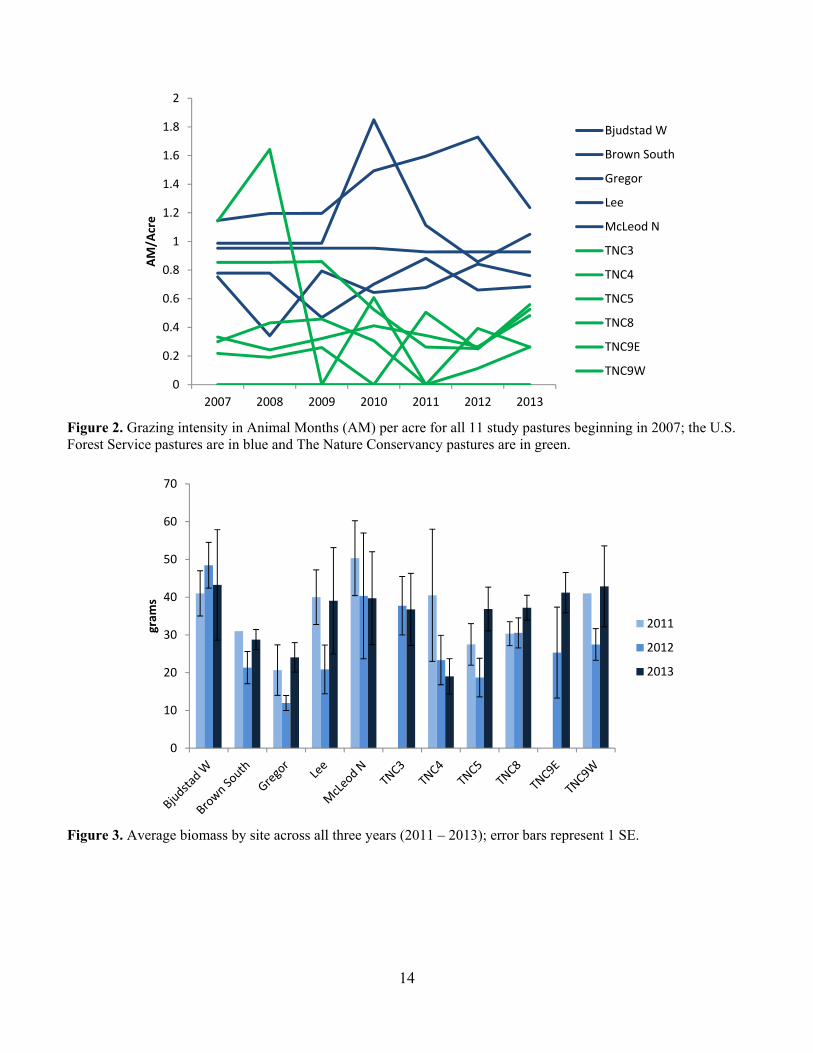
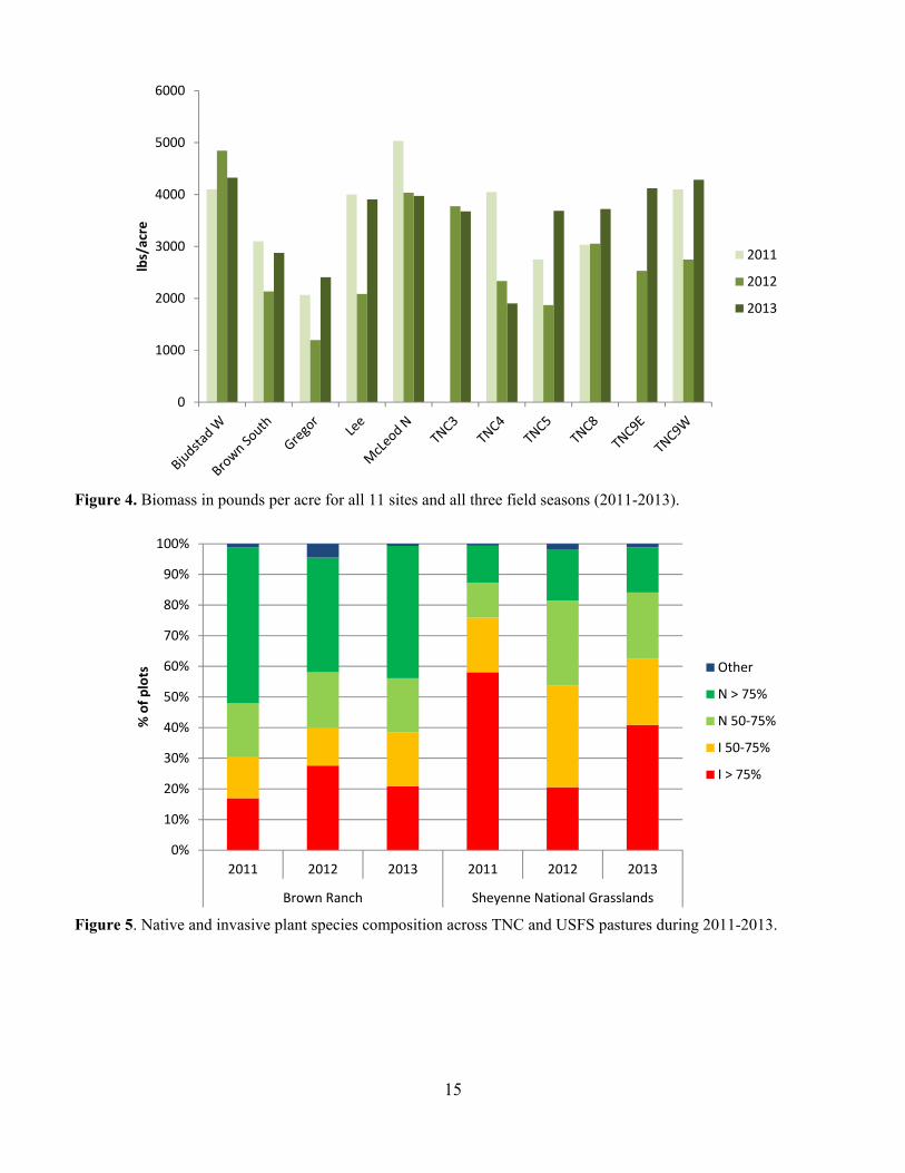
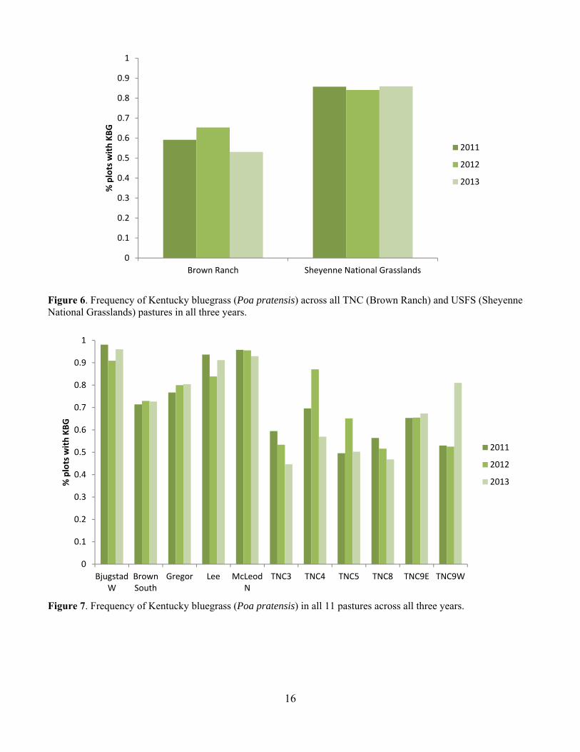
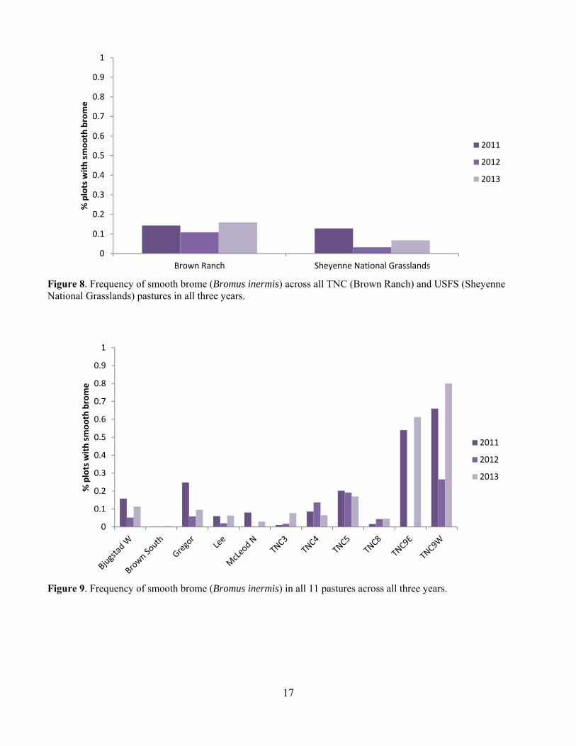
Sandpiper, Marbled Godwit and Bobolink (Fiske and Chandler 2011). We used the function pcount, which fits the N-mixture model (Royle 2004). We modeled each species individually. We evaluated year, date, date2, time and time2 as covariates on detection probability (Kery et al. 2005) and year, precipitation, grazing intensity, burn status, litter depth, the coefficient of variation of litter depth, and VOR as covariates on abundance (Table 1). We did not directly include observer in our models because observer was completely confounded by Year. We had different observers each year but within year the observer was the same for all counts. Therefore, Year is also a proxy for observer. To fit the models for each species, we first evaluated the model fit for all combinations of year, date, date2, time and time2 on detection probability with no covariates on abundance (Kery et al. 2005). We used AIC to select the top model. We then used stepwise forward selection to choose abundance covariates (Kery et al. 2013). We accepted a new term in the model only if the model had a lower AIC term and the model passed a likelihood ratio goodness of fit test (Kery et al. 2005). If we had a bad goodness of fit for all variables, we reran the model using negative binomial and zero inflated distributions. To assess goodness of fit for the top model, for each species we generated 100 replicate data sets using the parameter estimates from the AIC-best model. For each replicate data set, parameters were estimated and three fit statistics were computed: sum-of-squared errors, Freeman-Tukey, and chi-square. For each of the three methods, the group of simulated fit statistics formed the reference distribution to which the observed fit statistics were compared (Dixon 2002). Results and Discussion Grazing Intensity Grazing intensity spanned the range from 0 animal months/acre (AM/acre) to about 1.8 AM/acre over the course of the study (Fig. 2). At the start of the study in 2011, the grazing intensity on TNC pastures had been reduced below that of the USFS pastures and remained consistently lower for the duration of the project. Biomass Productivity We did not observe any strong trends in biomass productivity across ownerships (Fig. 3). Productivity on TNC pastures was comparable with the productivity on the USFS pastures. We did generally observe lower productivity on most pastures in 2012, which was a particularly dry year. We include here the summary in grams and in lbs/acre, because lbs/acre is used to calculate stocking densities (Fig. 4). Vegetation Composition Overall, TNC pastures had a higher percent cover of native dominated vegetation than the USFS pastures (Fig. 5). We see some variability in cover of invasive species that is likely related to variability in plant community expression under different weather conditions across the field seasons. Three of the most common invasive species were Kentucky bluegrass (Poa pratensis), smooth brome (Bromus inermis) and leafy spurge (Euphorbia esula). Kentucky bluegrass was by far the most frequently occurring invasive species across both TNC and USFS pastures (Fig. 6). Kentucky bluegrass does very well under grazing pressure (DeKeyser et al. 2013) and was more common on USFS pastures than TNC. By pasture, Kentucky bluegrass reaches near 100% occurrence on a couple of the USFS pastures and is over 40% occurrence on all pastures in all years (Fig. 7). Smooth brome is another invasive cool-season grass that is of great concern in the northern prairies (Grant et al. 2009, DeKeyser et al. 2013). Smooth brome was not nearly as common as Kentucky bluegrass and was generally more common in TNC pastures than USFS pastures (Figs. 8 & 9). Generally, smooth brome did not occur on more than 30% of the plots in a pasture with the exception of TNC 9E and TNC 9W (Fig. 9). On TNC 9 smooth brome was generally over 50% occurrence with a dramatic decrease in 2012 after a spring burn. Late spring burning has been shown to reduce smooth brome but the effects of grazing on brome are less clear (Bolwahn Salesman and Thomsen 2011).

5

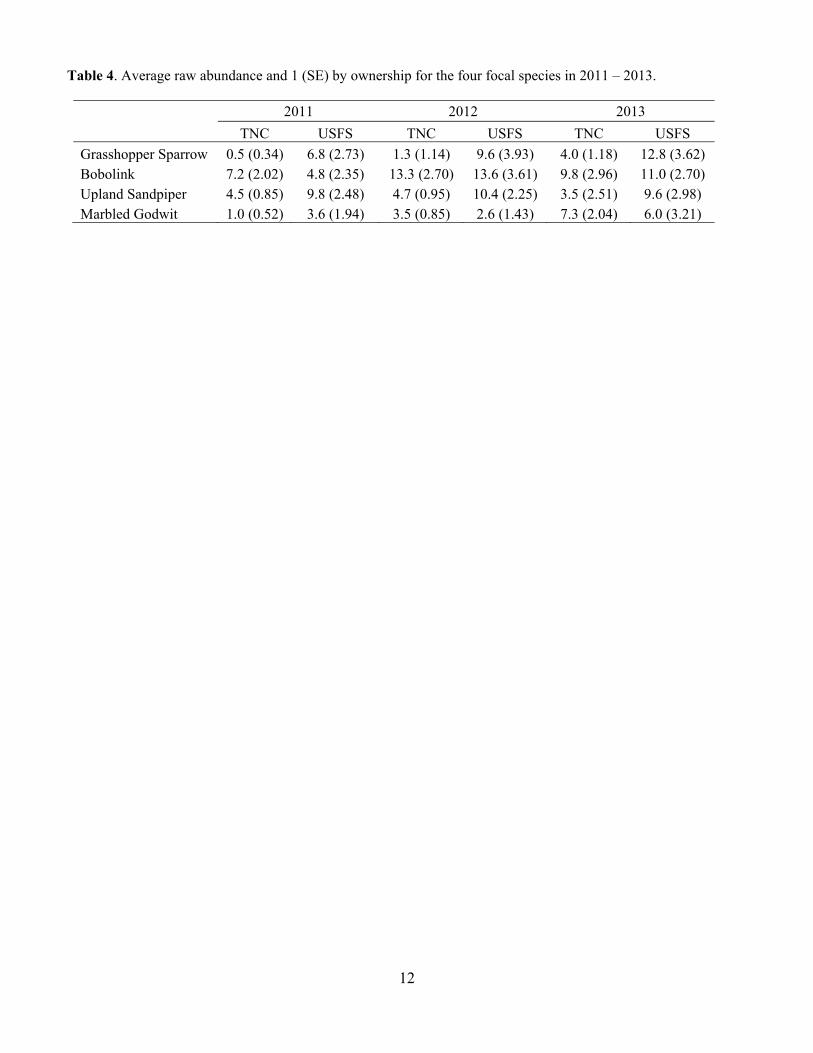
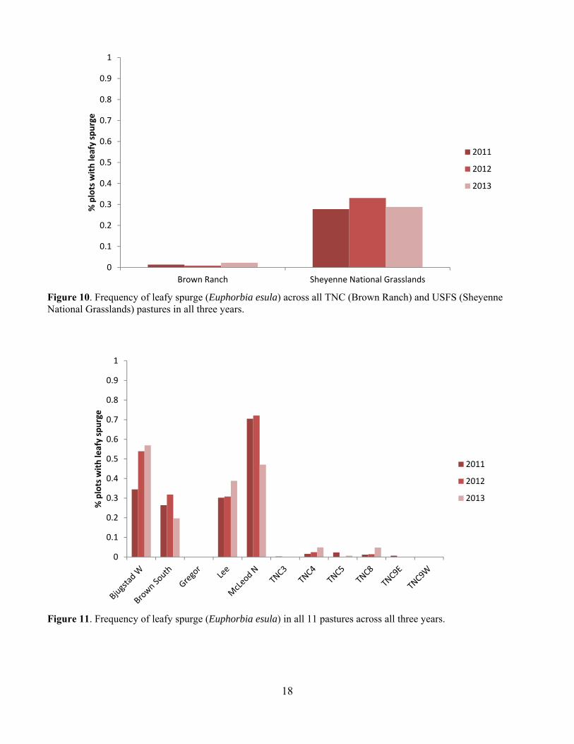
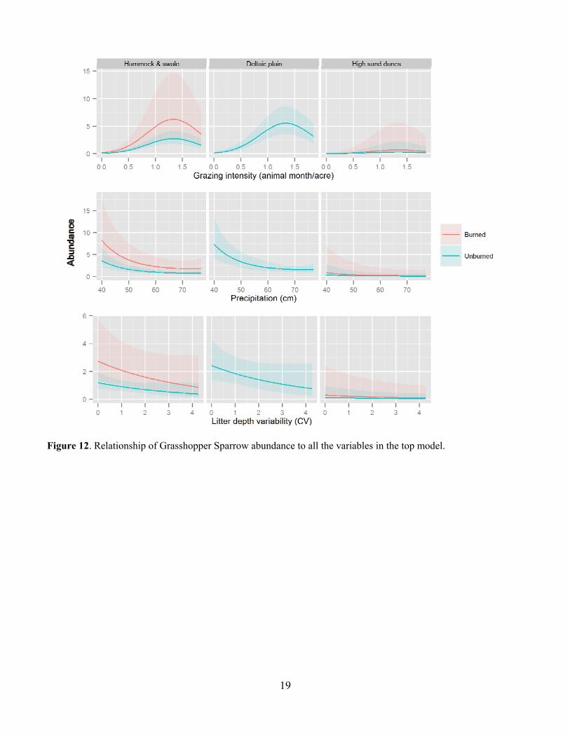
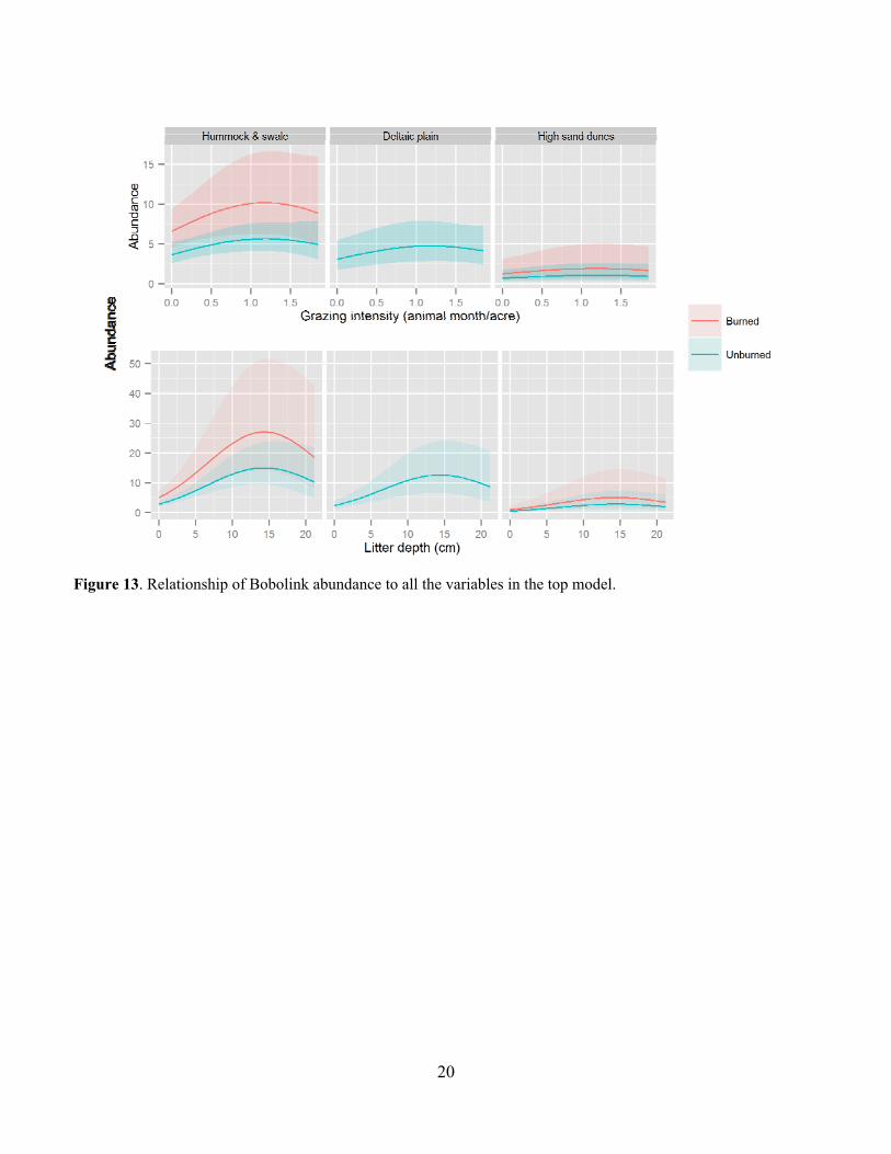
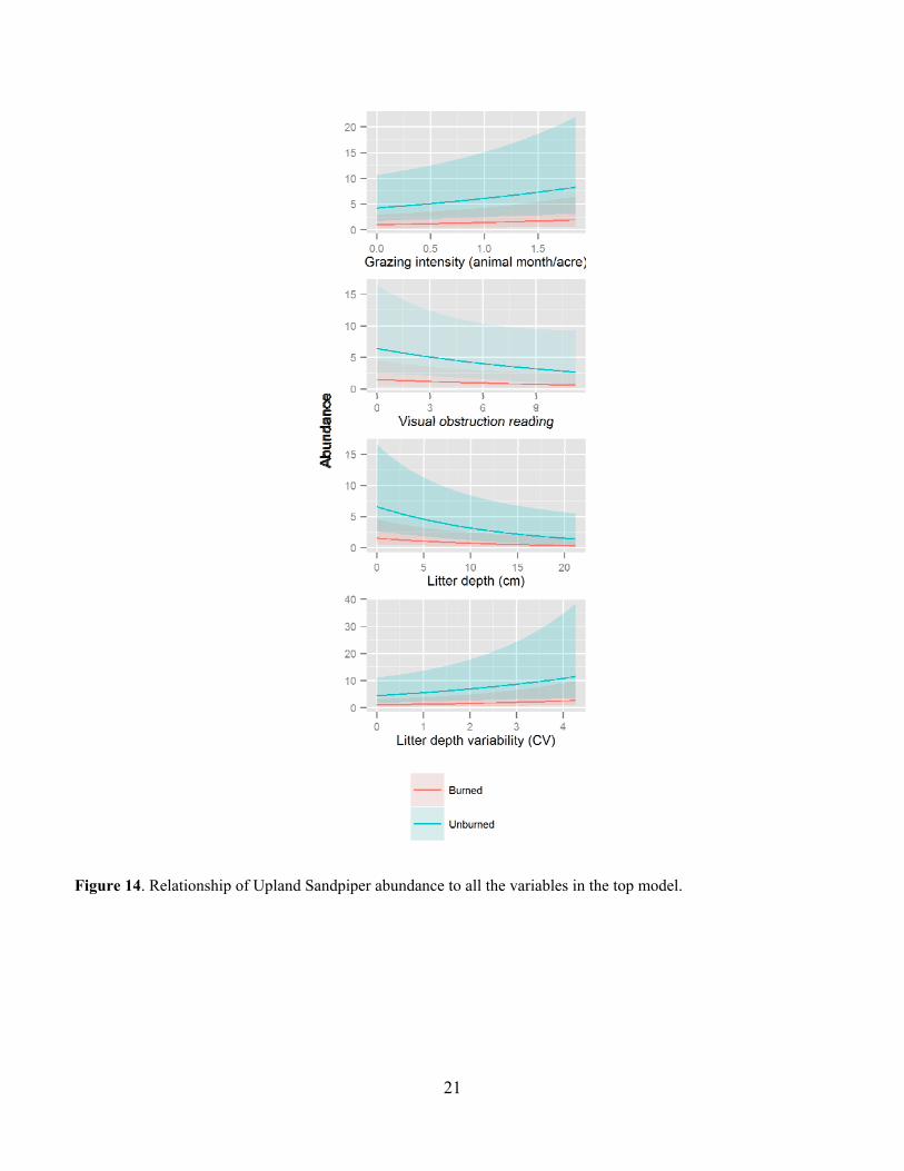
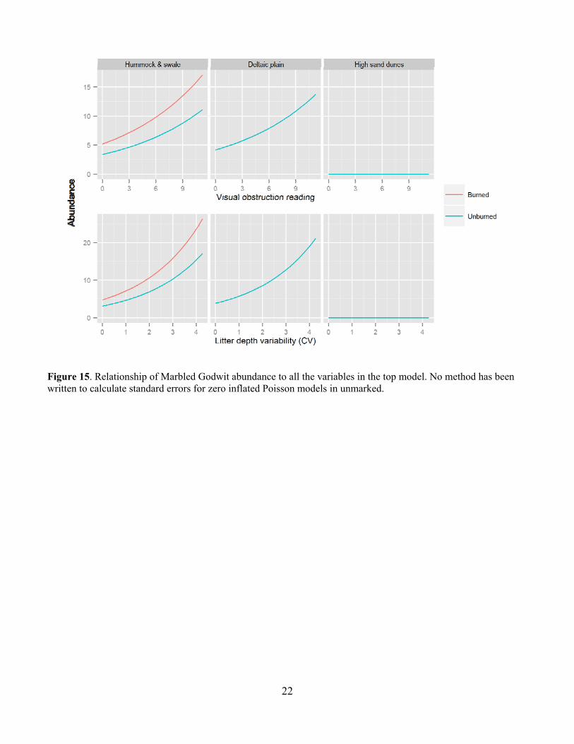
Leafy spurge was also a common invasive species in many of the pastures and was much more common on USFS pastures at around 30% occurrence than on TNC pastures at less than 5% occurrence (Fig. 10). Leafy spurge was fairly common on all but the Gregor USFS pasture (Fig. 11). Bird Abundance and Community Composition We detected 67 species across all years and all pastures, not including waterfowl species (Table 2). We detected 60 species in the TNC pastures and 59 species on the USFS pastures (Table 3). Of the four focal species, Bobolinks were the most ubiquitous species, detected on all pastures and in generally higher abundance (Table 4). Grasshopper Sparrows were much more common on the USFS pastures and increased in abundance each year. Upland Sandpipers were also detected on all pastures with the highest numbers seen on the USFS pastures. Marbled Godwits were not as common in general but saw an increase in abundance in 2013. For all four species, the AIC-best model fit adequately. All three parameters evaluated for detection probability were included in the top model for at least one species (Table 5). Date and the quadratic effect of date were included in all models but detection probability did not decline during the field season for all species. Time since sunrise and year were each included in the top model for three of the four species. Time since sunrise did not influence detection probability for Marbled Godwits, and year did not influence the detection probability for Upland Sandpipers. The strongest predictor of Grasshopper Sparrow abundance was grazing intensity (Table 5). Grasshopper Sparrows were generally positively related to grazing intensity, but the inclusion of the quadratic term for grazing intensity suggests a decrease in Grasshopper Sparrow abundance at the highest grazing intensities (Fig. 12). This is consistent with other studies that have found grazing to favor higher abundances of Grasshopper Sparrows in the eastern part of its distribution where vegetation is taller and more dense (Dechant et al. 1998 (revised 2002)). Abundance of Grasshopper Sparrows was higher on the deltaic plain ecological site and burned areas. Grasshopper Sparrow abundance increased as precipitation decreased during the three years of the study, which is consistent with their preference for the drier deltaic plain ecological sites. Finally, Grasshopper Sparrows had a negative relationship with litter depth, which is consistent with their positive association with grazing intensity but this effect was not strong or statistically significant. The top model for the Bobolink included the effects of litter depth, ESD, burning and grazing (Table 5). Bobolinks were generally positively related to litter depth, but the inclusion of the quadratic term suggests a decrease in abundance at the highest levels of litter depth (Fig. 13). This is consistent with previous reports that Bobolink abundance generally declines the year of a burn when litter is greatly reduced (Dechant et al. 1999 (revised 2001)). Bobolink abundance was also much higher on the hummock and swale and deltaic plain ecological sites than the high sand dunes. Finally, Bobolinks were positively related to grazing intensity but the relationship was weak. The top model for the Upland Sandpiper included grazing intensity, burning, litter depth, variability in litter depth and VOR (Table 5). The strongest predictor for Upland Sandpiper abundance was burning with lower abundances in recently burned areas (Fig. 14). However, they also had a positive relationship with grazing intensity and variability in litter depth along with a negative relationship with total litter depth and VOR. Taken together, these relationships are suggestive of higher abundances in areas with more open, sparse vegetation. Upland Sandpipers have been found to avoid recently burned areas for nesting and like many species with precocial young, they require habitat heterogeneity for nesting and brood rearing needs (Dechant et al. 1999 (revised 2002)). Three of the parameter estimates in the top model were significantly different from zero (Table 5). Marbled Godwit abundance was higher in recently burned areas and areas with greater VOR and more variability in litter depth (Fig. 15). Marbled Godwits nest in scrapes on the ground so recently burned areas likely provide better nest sites with low levels of residual vegetation on the ground (Dechant et al. 1998 (revised 2001)). Communication of Results Annual reports have been shared with the USFS office in Lisbon, ND. Preliminary results from this project were presented at the Ecological Society of American conference in August of 2013 in Minneapolis, MN and at the All

6

Science Meeting for The Nature Conservancy in December of 2013 in San Jose, CA. The final report will be shared widely, and a peer-reviewed publication is in prep for the final results. Acknowledgements We thank the North Dakota State Wildlife Grants Program for generously supporting this project with Wildlife and Sport Fish Restoration Program funds, and the U. S. Forest Service and the Sheyenne National Grasslands for granting access and cooperating with data collection for the project. We thank The Nature Conservancy and Eric Hoff at Brown Ranch for providing housing and logistical support throughout the project. We also thank Jennifer Benson, Heather Funk, Danielle Hernandez, Allison Beardsley, Brittany Sheridan, Maggi Sliwinski, Brittany Irle, Cara Bush and Jenna Daub for field data collection and Dr. Chris Merkord for assistance with data analysis. Literature Cited Bolwahn Salesman, J. and M. Thomsen. 2011. Smooth brome (Bromus inermis) in tallgrass prairies: a

review of control methods and future research directions. Ecological Restoration 29:374-381. Bragg, T. B. 1995. The physical environment of Great Plains grasslands. Pages 49-81 in A. Joern and K.

H. Keeler, editors. The Changing Prairie. Oxford University Press, New York. Chapman, R. N., D. M. Engle, R. E. Masters, and D. M. Leslie, Jr. 2004. Grassland vegetation and bird

communities in the southern Great Plains of North America. Agriculture, Ecosystems and Environment 104:577-585.

Dechant, J. A., M. F. Dinkins, D. H. Johnson, L. D. Igl, C. M. Goldade, B. D. Parkin, and B. R. Euliss. 1999 (revised 2002). Effects of management practices on grassland birds: Upland Sandpiper. Northern Prairie Wildlife Research Center, Jamestown, ND. 34 pages. http://www.npwrc.usgs.gov/resource/literatr/grasbird/larb/larb.htm

Dechant, J. A., M. L. Sondreal, D. H. Johnson, L. D. Igl, C. M. Goldade, M. P. Nenneman, and B. R. Euliss. 1998 (revised 2001). Effects of management practices on grassland birds: Marbled Godwit. Northern Prairie Wildlife Research Center, Jamestown, ND. 11 pages. http://www.npwrc.usgs.gov/resource/literatr/grasbird/larb/larb.htm

Dechant, J. A., M. L. Sondreal, D. H. Johnson, L. D. Igl, C. M. Goldade, M. P. Nenneman, and B. R. Euliss. 1998 (revised 2002). Effects of management practices on grassland birds: Grasshopper Sparrow. Northern Prairie Wildlife Research Center, Jamestown, ND. 28 pages. http://www.npwrc.usgs.gov/resource/literatr/grasbird/larb/larb.htm

Dechant, J. A., M. L. Sondreal, D. H. Johnson, L. D. Igl, C. M. Goldade, A. L. Zimmerman, and B. R. Euliss. 1999 (revised 2001). Effects of management practices on grassland birds: Bobolink. Northern Prairie Wildlife Research Center, Jamestown, ND. 24 pages. http://www.npwrc.usgs.gov/resource/literatr/grasbird/larb/larb.htm.

DeKeyser, E. S., M. Meehan, G. K. Clambey, and K. Krabbenhoft. 2013. Cool season invasive grasses in northern Great Plains natural areas. Natural Areas Journal 33:81-90.

Dixon, P. M. 2002. Bootstrap resampling. Encyclopedia of Environmetrics 1:212-220. Fisher, R. J. and S. K. Davis. 2010. From Wiens to Robel: a review of grassland-bird habitat selection.

Journal of Wildlife Management 74:265-273. Fiske, I. J. and R. B. Chandler. 2011. unmarked: an R package for fitting hierarchical models of wildlife

occurrence and abundance. Journal of Statistical Software 43:1-23. Fuhlendorf, S. D., W. C. Harrel, D. M. Engle, R. G. Hamilton, C. A. Davis, and D. M. Leslie, Jr. 2006.

Should heterogeneity be the basis for conservation? Grassland bird response to fire and grazing. Ecological Applications 16:1706-1716.

Grant, T. A., B. Flanders-Wanner, T. L. Shaffer, R. K. Murphy, and G. A. Knutsen. 2009. An emerging crisis across northern prairie refuges: prevalence of invasive plants and a plan for adaptive management. Ecological Restoration 27:58-65.

7

Grant, T. A., E. M. Madden, T. L. Shaffer, and J. S. Dockens. 2010. Effects of prescribed fire on vegetation and passerine birds in northern mixed-grass prairie. Journal of Wildlife Management 74:1841-1851.

Hovick, T. J., J. R. Miller, S. J. Dinsmore, D. M. Engle, D. M. Debinski, and S. D. Fuhlendorf. 2012. Effects of fire and grazing on grasshopper sparrow nest survival. Journal of Wildlife Management 76:19-27.

Kery, M., G. Guillera-Arroita, and J. J. Lahoz-Monfort. 2013. Analysing and mapping species range dynamics using occupancy models. Journal of Biogeography 40:1463-1474.

Kery, M., J. A. Royle, and H. Schmid. 2005. Modeling avian abundance from replicated counts using binomial mixture models. Ecological Applications 15:1450-1461.

Robel, R. J., J. N. Briggs, A. D. Dayton, and L. C. Hulbert. 1970. Relationships between visual obstruction measurements and weight of grassland vegetation. Journal of Range Management 23:295-297.

Royle, J. A. 2004. N-mixture models for estimating population size from spatially replicated counts. Biometrics 60:108-115.

Team, R. C. 2014. R: a language and environment for statistical computing. R Foundation for Statistical Computing. http://www.R-project.org.

8

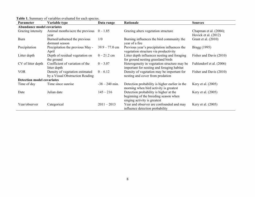
Table 1. Summary of variables evaluated for each species. Parameter Variable type Data range Rationale Sources Abundance model covariates Grazing intensity Animal months/acre the previous

year 0 – 1.85 Grazing alters vegetation structure Chapman et al. (2004);

Hovick et al. (2012) Burn Burned/unburned the previous

dormant season 1/0 Burning influences the bird community the

year of a fire Grant et al. (2010)

Precipitation Precipitation the previous May - April

39.9 – 77.0 cm Previous year’s precipitation influences the vegetation structure via productivity

Bragg (1995)

Litter depth Depth of residual vegetation on the ground

0 – 21.2 cm Litter depth influences nesting and foraging for ground nesting grassland birds

Fisher and Davis (2010)

CV of litter depth Coefficient of variation of the litter depth

0 – 3.07 Heterogeneity in vegetation structure may be important for nesting and foraging habitat

Fuhlendorf et al. (2006)

VOR Density of vegetation estimated by a Visual Obstruction Reading

0 – 6.12 Density of vegetation may be important for nesting and cover from predation

Fisher and Davis (2010)

Detection model covariates Time of day Time since sunrise -38 – 240 min. Detection probability is higher earlier in the

morning when bird activity is greatest Kery et al. (2005)

Date Julian date 145 – 216 Detection probability is higher at the beginning of the breeding season when singing activity is greatest

Kery et al. (2005)

Year/observer Categorical 2011 – 2013 Year and observer are confounded and may influence detection probability

Kery et al. (2005)

9

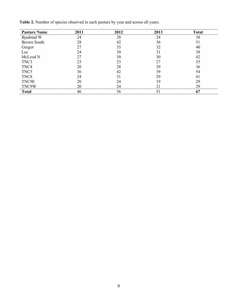
Table 2. Number of species observed in each pasture by year and across all years. Pasture Name 2011 2012 2013 Total Bjudstad W 24 28 24 38 Brown South 28 42 36 51 Gregor 27 35 32 40 Lee 24 30 31 38 McLeod N 27 30 30 42 TNC3 23 23 27 35 TNC4 20 28 29 36 TNC5 36 42 39 54 TNC8 24 31 29 41 TNC9E 20 24 19 29 TNC9W 20 24 21 29 Total 46 56 51 67

10

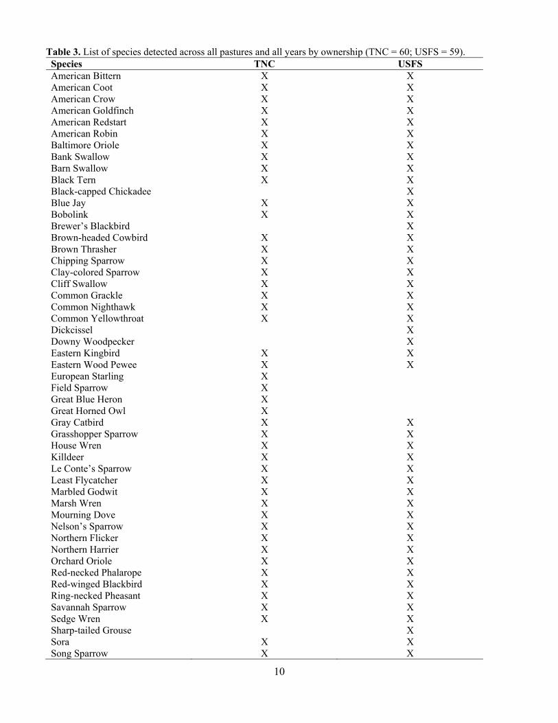
Table 3. List of species detected across all pastures and all years by ownership (TNC = 60; USFS = 59). Species TNC USFS American Bittern X X American Coot X X American Crow X X American Goldfinch X X American Redstart X X American Robin X X Baltimore Oriole X X Bank Swallow X X Barn Swallow X X Black Tern X X Black-capped Chickadee X Blue Jay X X Bobolink X X Brewer’s Blackbird X Brown-headed Cowbird X X Brown Thrasher X X Chipping Sparrow X X Clay-colored Sparrow X X Cliff Swallow X X Common Grackle X X Common Nighthawk X X Common Yellowthroat X X Dickcissel X Downy Woodpecker X Eastern Kingbird X X Eastern Wood Pewee X X European Starling X Field Sparrow X Great Blue Heron X Great Horned Owl X Gray Catbird X X Grasshopper Sparrow X X House Wren X X Killdeer X X Le Conte’s Sparrow X X Least Flycatcher X X Marbled Godwit X X Marsh Wren X X Mourning Dove X X Nelson’s Sparrow X X Northern Flicker X X Northern Harrier X X Orchard Oriole X X Red-necked Phalarope X X Red-winged Blackbird X X Ring-necked Pheasant X X Savannah Sparrow X X Sedge Wren X X Sharp-tailed Grouse X Sora X X Song Sparrow X X

11

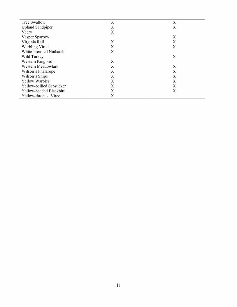
Tree Swallow X X Upland Sandpiper X X Veery X Vesper Sparrow X Virginia Rail X X Warbling Vireo X X White-breasted Nuthatch X Wild Turkey X Western Kingbird X Western Meadowlark X X Wilson’s Phalarope X X Wilson’s Snipe X X Yellow Warbler X X Yellow-bellied Sapsucker X X Yellow-headed Blackbird X X Yellow-throated Vireo X

12

Table 4. Average raw abundance and 1 (SE) by ownership for the four focal species in 2011 – 2013.

2011 2012 2013

TNC USFS TNC USFS TNC USFS

Grasshopper Sparrow 0.5 (0.34) 6.8 (2.73) 1.3 (1.14) 9.6 (3.93) 4.0 (1.18) 12.8 (3.62) Bobolink 7.2 (2.02) 4.8 (2.35) 13.3 (2.70) 13.6 (3.61) 9.8 (2.96) 11.0 (2.70) Upland Sandpiper 4.5 (0.85) 9.8 (2.48) 4.7 (0.95) 10.4 (2.25) 3.5 (2.51) 9.6 (2.98) Marbled Godwit 1.0 (0.52) 3.6 (1.94) 3.5 (0.85) 2.6 (1.43) 7.3 (2.04) 6.0 (3.21)

13

Table 5. Standardized parameter estimates for N-mixture models for four focal species in the Sheyenne River Delta, North Dakota. Parameter estimates in bold are significantly different from zero. Grasshopper Sparrow Bobolink Upland Sandpiper Marbled Godwit Mean SE 0.025 0.975 Mean SE 0.025 0.975 Mean SE 0.025 0.975 Mean SE 0.025 0.975Abundance model Intercept 0.66 0.26 0.16 1.16 1.46 0.27 0.93 1.99 1.67 0.46 0.77 2.57 2.12 0.76 0.63 3.60AM/acre 1.49 0.21 1.08 1.90 0.17 0.07 0.03 0.31 0.18 0.08 0.03 0.33 - - - -AM/acre2 -0.52 0.09 -0.70 -0.35 -0.08 0.05 -0.17 0.01 - - - - - - - -Burn 0.83 0.35 0.14 1.52 0.59 0.19 0.23 0.96 -1.46 0.34 -2.14 -0.79 0.43 0.21 0.01 0.85Precipitation -0.66 0.25 -1.15 -0.17 - - - - - - - - - - - -Precipitation2 0.49 0.34 -0.18 1.16 - - - - - - - - - - - -Litter depth - - - - 0.56 0.09 0.38 0.75 -0.22 0.09 -0.40 -0.04 - - - -Litter depth2 - - - - -0.07 0.02 -0.11 -0.04 - - - - - - - -CV litter depth -0.16 0.10 -0.36 0.03 - - - - 0.14 0.07 0.00 0.28 0.24 0.07 0.10 0.38VOR - - - - - - - - -0.11 0.08 -0.27 0.04 0.16 0.07 0.01 0.30ESD - HSD -2.94 1.02 -4.93 -0.95 -1.51 0.51 -2.50 -0.52 - - - - -8.66 20.46 -48.77 31.45ESD - HS -0.71 0.17 -1.04 -0.38 0.17 0.23 -0.28 0.62 - - - - -0.21 0.33 -0.86 0.44Detection model Intercept -1.18 0.37 -1.90 -0.46 -1.82 0.21 -2.24 -1.40 -1.63 0.55 -2.70 -0.56 -4.22 0.76 -5.70 -2.73Time of day -0.22 0.06 -0.35 -0.10 0.22 0.05 0.13 0.31 0.24 0.07 0.11 0.37 - - - -Time of day2 0.05 0.07 -0.07 0.18 - - - - -0.35 0.07 -0.48 -0.22 - - - -Date 0.08 0.07 -0.05 0.21 -0.61 0.07 -0.75 -0.47 0.46 0.08 0.31 0.61 -3.68 0.54 -4.73 -2.62Date2 0.04 0.06 -0.07 0.15 -0.43 0.07 -0.57 -0.29 -0.53 0.07 -0.66 -0.40 -1.69 0.33 -2.34 -1.042012 1.34 0.41 0.53 2.14 0.38 0.17 0.06 0.71 - - - - -0.21 0.33 -0.86 0.442013 -0.29 0.51 -1.29 0.70 0.57 0.19 0.21 0.94 - - - - 0.43 0.29 -0.14 0.99

14

Figure 2. Grazing intensity in Animal Months (AM) per acre for all 11 study pastures beginning in 2007; the U.S. Forest Service pastures are in blue and The Nature Conservancy pastures are in green.

Figure 3. Average biomass by site across all three years (2011 – 2013); error bars represent 1 SE.

0

0.2

0.4

0.6

0.8

1

1.2

1.4

1.6

1.8

2

2007 2008 2009 2010 2011 2012 2013

AM/A

cre

Bjudstad W

Brown South

Gregor

Lee

McLeod N

TNC3

TNC4

TNC5

TNC8

TNC9E

TNC9W

0

10

20

30

40

50

60

70

gram

s

2011

2012

2013

15

Figure 4. Biomass in pounds per acre for all 11 sites and all three field seasons (2011-2013).

Figure 5. Native and invasive plant species composition across TNC and USFS pastures during 2011-2013.

0

1000

2000

3000

4000

5000

6000

lbs/acre

2011

2012

2013

0%

10%

20%

30%

40%

50%

60%

70%

80%

90%

100%

2011 2012 2013 2011 2012 2013

Brown Ranch Sheyenne National Grasslands

% of plots Other

N > 75%

N 50‐75%

I 50‐75%

I > 75%

16

Figure 6. Frequency of Kentucky bluegrass (Poa pratensis) across all TNC (Brown Ranch) and USFS (Sheyenne National Grasslands) pastures in all three years.

Figure 7. Frequency of Kentucky bluegrass (Poa pratensis) in all 11 pastures across all three years.

0

0.1

0.2

0.3

0.4

0.5

0.6

0.7

0.8

0.9

1

Brown Ranch Sheyenne National Grasslands

% plots with KBG

2011

2012

2013

0

0.1

0.2

0.3

0.4

0.5

0.6

0.7

0.8

0.9

1

BjugstadW

BrownSouth

Gregor Lee McLeodN

TNC3 TNC4 TNC5 TNC8 TNC9E TNC9W

% plots with KBG

2011

2012

2013

17

Figure 8. Frequency of smooth brome (Bromus inermis) across all TNC (Brown Ranch) and USFS (Sheyenne National Grasslands) pastures in all three years.

Figure 9. Frequency of smooth brome (Bromus inermis) in all 11 pastures across all three years.

0

0.1

0.2

0.3

0.4

0.5

0.6

0.7

0.8

0.9

1

Brown Ranch Sheyenne National Grasslands

% plots with smooth brome

2011

2012

2013

0

0.1

0.2

0.3

0.4

0.5

0.6

0.7

0.8

0.9

1

% plots with smooth brome

2011

2012

2013

18

Figure 10. Frequency of leafy spurge (Euphorbia esula) across all TNC (Brown Ranch) and USFS (Sheyenne National Grasslands) pastures in all three years.

Figure 11. Frequency of leafy spurge (Euphorbia esula) in all 11 pastures across all three years.

0

0.1

0.2

0.3

0.4

0.5

0.6

0.7

0.8

0.9

1

Brown Ranch Sheyenne National Grasslands

% plots with leafy spurge

2011

2012

2013

0

0.1

0.2

0.3

0.4

0.5

0.6

0.7

0.8

0.9

1

% plots with leafy spurge

2011

2012

2013

19

Figure 12. Relationship of Grasshopper Sparrow abundance to all the variables in the top model.

20

Figure 13. Relationship of Bobolink abundance to all the variables in the top model.

21

Figure 14. Relationship of Upland Sandpiper abundance to all the variables in the top model.

22

Figure 15. Relationship of Marbled Godwit abundance to all the variables in the top model. No method has been written to calculate standard errors for zero inflated Poisson models in unmarked.