Normalizing economic loss from natural disasters - Centre for

The Munich Re Programme: Evaluating the Economics

of Climate Risks and Opportunities in the Insurance Sector

Normalizing economic loss from natural disasters: a global analysis

Eric Neumayer and Fabian Barthel

November 2010

Centre for Climate Change Economics and Policy Working Paper No. 41

Munich Re Programme Technical Paper No. 6

Grantham Research Institute on Climate Change and the Environment

Working Paper No. 31

The Centre for Climate Change Economics and Policy (CCCEP) was established by the University of Leeds and the London School of Economics and Political Science in 2008 to advance public and private action on climate change through innovative, rigorous research. The Centre is funded by the UK Economic and Social Research Council and has five inter-linked research programmes:

1. Developing climate science and economics 2. Climate change governance for a new global deal 3. Adaptation to climate change and human development 4. Governments, markets and climate change mitigation 5. The Munich Re Programme - Evaluating the economics of climate risks and

opportunities in the insurance sector (funded by Munich Re) More information about the Centre for Climate Change Economics and Policy can be found at: http://www.cccep.ac.uk. The Munich Re Programme is evaluating the economics of climate risks and opportunities in the insurance sector. It is a comprehensive research programme that focuses on the assessment of the risks from climate change and on the appropriate responses, to inform decision-making in the private and public sectors. The programme is exploring, from a risk management perspective, the implications of climate change across the world, in terms of both physical impacts and regulatory responses. The programme draws on both science and economics, particularly in interpreting and applying climate and impact information in decision-making for both the short and long term. The programme is also identifying and developing approaches that enable the financial services industries to support effectively climate change adaptation and mitigation, through for example, providing catastrophe insurance against extreme weather events and innovative financial products for carbon markets. This programme is funded by Munich Re and benefits from research collaborations across the industry and public sectors. The Grantham Research Institute on Climate Change and the Environment was established by the London School of Economics and Political Science in 2008 to bring together international expertise on economics, finance, geography, the environment, international development and political economy to create a world-leading centre for policy-relevant research and training in climate change and the environment. The Institute is funded by the Grantham Foundation for the Protection of the Environment, and has five research programmes:

1. Use of climate science in decision-making 2. Mitigation of climate change (including the roles of carbon markets and low-

carbon technologies) 3. Impacts of, and adaptation to, climate change, and its effects on development 4. Governance of climate change 5. Management of forests and ecosystems

More information about the Grantham Research Institute on Climate Change and the Environment can be found at: http://www.lse.ac.uk/grantham. This working paper is intended to stimulate discussion within the research community and among users of research, and its content may have been submitted for publication in academic journals. It has been reviewed by at least one internal referee before publication. The views expressed in this paper represent those of the author(s) and do not necessarily represent those of the host institutions or funders.

Normalizing Economic Loss from Natural Disasters: A Global Analysis

Accepted for publication and forthcoming in Global Environmental Change, Vol. 21, Issue 1, 2011

Eric Neumayer∗∗∗∗ and Fabian Barthel Department of Geography and Environment and The Grantham Research Institute on Climate Change and the Environment, London School of Economics and Political Science, Houghton Street, London WC2A 2AE, U.K. Fax: +44 (0)20 7955 7412 Tel: +44 (0)20 7955 7598

∗ Corresponding author (email: [email protected]). The authors acknowledge financial and other support from the Munich Re Programme “Evaluating the Economics of Climate Risks & Opportunities in the Insurance Sector” at LSE. All views expressed are our own and do not represent the views of Munich Re. We thank Jan Eichner, Eberhard Faust, Peter Hoeppe, Roger Pielke Jr., Nicola Ranger, Lenny Smith and an anonymous referee for many helpful comments. All errors are ours.

1

Normalizing Economic Loss from Natural Disasters: A Global Analysis

Abstract

Climate change is likely to lead to an increase in the frequency and/or intensity of

certain types of natural hazards, if not globally, then at least in certain regions. All

other things equal, this should lead to an increase in the economic toll from natural

disasters over time. Yet, all other things are not equal since affected areas become

wealthier over time and rational individuals and governments undertake defensive

mitigation measures, which requires normalizing economic losses if one wishes to

analyze trends in economic loss from natural disasters for detecting a potential climate

change signal. In this article, we argue that the conventional methodology for

normalizing economic loss is problematic since it normalizes for changes in wealth

over time, but fails to normalize for differences in wealth across space at any given

point of time. We introduce an alternative methodology that overcomes this problem

in theory, but faces many more problems in its empirical application. Applying,

therefore, both methods to the most comprehensive existing global dataset of natural

disaster loss, in general we find no significant upward trends in normalized disaster

damage over the period 1980 to 2009 globally, regionally, for specific disasters or for

specific disasters in specific regions. Due to our inability to control for defensive

mitigation measures, one cannot infer from our analysis that there have definitely not

been more frequent and/or more intensive weather-related natural hazards over the

study period already. Moreover, it may still be far too early to detect a trend if human-

induced climate change has only just started and will gain momentum over time.

2

1. Introduction

Has economic damage from natural disasters increased over time? This is a question

of high policy relevance for mainly two reasons. First, if it has then this could require

a policy response in terms of disaster risk management and disaster damage

mitigation and prevention. Second, an increasing trend of damage from natural

disasters could point in the direction that climatic changes may be the driving force,

which would have implications for the debate on reducing greenhouse gas emissions

(Bouwer 2009; Schmidt, Kemfert and Höppe 2009).1 This question has recently

attracted some broader media attention when critics accused both the Inter-

governmental Panel on Climate Change (IPCC) and the Stern (2007) Review of

allegedly reporting selected pieces of evidence in support of such a trend.2

A potential climate change signal is not easily detected from data of economic

loss from natural disasters, however. One cannot simply look at inflation-adjusted

damages from natural disasters and test for a time trend therein. While such an

analysis would be interesting for other reasons, any trend found may simply be due to

the fact that areas affected by natural disasters have become wealthier over time. For

example, people often move to disaster-prone areas such as floodplanes and coastal

areas because other characteristics of these areas attract them, which provide a higher

expected benefit than the expected cost following from damage in the uncertain event

of natural disaster. Even in the absence of migration, existing populations in affected

areas are bound to increase over time, while property values are bound to rise. Hence,

any increase in natural disaster damage may be entirely due to an increase in what can

potentially be destroyed, i.e. an increase in exposed wealth, rather than because of an

1 For example, IPCC (2001: 13) claims that ‘part of the observed upward trend in disaster losses

over the past 50 years is linked to socioeconomic factors (…), and part is linked to climatic factors, such as the observed changes in precipitation and flooding events’.

2 See, for example, Pielke (2007).

3

increase in the frequency and/or intensity (potential destructive power) of natural

hazards.3 Even then, a policy response may be required of course – for example, in the

form of discouraging people from migrating to disaster-prone areas and undertaking

measures to protect the lives and property of existing people in such areas.

The question that has attraced more scholarly attention, however, is whether

even after adjusting for changes in wealth, there is still an increasing trend in natural

disaster damage over time. Certainly, if one is interested in analyzing whether

climatic change plays a role in increasing disaster damage, then this is the question to

address. Existing scholarship seemingly provides an exhaustive negative answer to

this question already, but there is a large amount of terra incognita in terms of

adequate regional- and hazard-specific loss analyses, partly because of unavailability

of data. Existing scholarship comes to the conclusion that while natural variability in

weather patterns can explain some of the variability in disaster losses (Pielke and

Landsea 1998; Katz 2002; Pielke et al. 2008; Schmidt, Kemfert and Höppe 2009),

there is no evidence for a rising long-term trend in so-called “normalized” disaster

damage, which is the damage after adjustments for wealth changes over time. To be

sure, even if a trend was detected, one needs to be careful in attributing such a trend to

anthropogenic climate change, i.e. climate change caused by man-made greenhouse

gas emissions, since natural climate variability could provide an alternative

explanation. For example, some studies find an upward trend in normalized damage

from hurricanes in the US since the 1970s (e.g., Schmidt, Kemfert and Höppe 2009) –

a trend, which may well be explained by natural variability in hurricane landfall.

There are three reasons why the topic of natural disaster loss normalization

needs to be studied further. First, the vast majority of existing studies have either 3 Hazards are events triggered by natural forces. They will turn into natural disasters if people

are exposed to the hazard and are not resilient to fully absorbing the impact without damage to life or property (Schwab, Eschelbach and Brower 2007).

4

analyzed losses in the United States (Pielke and Landsea 1998; Brooks and Doswell

2001; Nordhaus 2006; Pielke et al. 2008; Vranes and Pielke 2009; Schmidt, Kemfert

and Höppe 2009) or other countries (Raghavan and Rajseh 2003; Crompton and

McAeneney 2008) or a region (Pielke et al. 2003; Barredo 2009).4 It remains to be

seen whether what holds true for these individual countries or regions will hold for

other countries, other regions and the world as a whole. Second, the one study that has

looked at disaster damage on a global scale (Miller et al. 2008) suffers from the fact

that it had to resort to assembling loss estimates from a plethora of sources, which will

use very different criteria and which will produce data of very varied quality. Third,

the normalization methodology used by practically all existing studies is, we argue

here, incomplete in that it normalizes for changes over time, but fails to normalize for

differences in spatial location at any point of time. This article addresses all three

shortcomings by analyzing a global sample in addition to region-specific samples, by

using a comprehensive high-quality database and by employing, in addition to the

conventional method, a methodology that normalizes both for changes over time and

differences over space. In other words, this article makes both a contribution to the

substance and the methodology of the literature studying economic loss from natural

disasters.

Despite these differences in research design, we come to similar conclusions

as existing studies: whilst we find massive increases in non-normalized inflation-

adjusted natural disaster damage, there is no longer any evidence for an increasing

trend once each natural disaster event has been normalized. It is premature to interpret

these findings as evidence that climatic factors have not led to an increase in

normalized disaster damage. This is because defensive mitigating measures

4 Bouwer (2009) provides a comprehensive literature review.

5

undertaken by rational individuals and governments in response to more frequent

and/or more intensive natural hazards may have reduced natural disaster losses such

that these measures would mask any increasing trend in normalized disaster damage.

Unfortunately, it is impossible to adequately account for measures such as improved

early warning systems, better building qualities, heightened flood defences etc. It is

therefore impossible to say whether one would see an increasing trend in normalized

natural disaster damages in the absence of such measures.

This article is structured as follows: Section 2 outlines the conventional

approach to normalise disaster losses, while Section 3 discusses its limitations. Our

alternative method is presented in Section 4. Results of a global analysis and for

various regions and disaster types are shown in Section 5, using both normalization

approaches. Section 6 concludes with an emphasis on the caveats and limitations that

necessarily accompany our analysis. In particular, we stress that our inability to take

into account defensive mitigating measures implies that one cannot infer from our

analysis that there has been no actual increase in the frequency and/or intensity of

weather-related natural hazards. Our analysis therefore cannot be used to undermine

the case for reducing greenhouse gas emissions – based on the precautionary principle

and justified in part by a desire to prevent or reduce a potentially increasing trend in

economic loss from natural disasters in the future.

2. The conventional approach to normalizing natural disaster loss

The conventional approach to normalizing natural disaster loss can be credited to

Roger Pielke Jr. and co-authors (see Pielke and Landsea 1998, Pielke et al. 1999,

2003, 2008; Vraines and Pielke 2009). The typical equation to compute normalized

damage according to this approach is as follows:

6

s s s st t

t t t

GDPdeflator Population Wealth per capitaNormalized Damage Damage

GDPdeflator Population Wealth per capita= ⋅ ⋅ ⋅ (1)

where s is the (chosen) year one wishes to normalize to, t is the year in which damage

occurred, the Gross Domestic Product (GDP) deflator adjusts for inflation (i.e.,

change in producer prices), while the remaining two correction factors adjust for

changes in population and wealth per capita. In theory, the population and wealth

changes should be based on data from the exact areas affected by the natural disaster

in question. However, in practice it is often impossible to determine the exact areas or

information on these areas is difficult or impossible to get, so scholars typically resort

to using data from the country or, if they can, from sub-country administrative units

known to be affected (e.g., counties or states). Studies differ with respect to how

wealth per capita is measured. Some use data on the value of capital stocks (e.g.,

Pielke and Landsea 1998; Brooks and Doswell 2001; Vranes and Pielke 2009;

Schmidt, Kemfert and Höppe 2009) or the value of dwellings (Crompton and

McAneney 2008; Pielke et al. 2008), others, often for lack of data, simply GDP per

capita (e.g., Raghavan and Rajseh 2003; Pielke et al. 2003; Nordhaus 2006; Miller et

al. 2008; Barredo 2009). With more than one disaster per year, the measure of disaster

loss per year is the sum of normalized damages from each disaster as per equation (1).

Pielke et al. (2008) justify the conventional normalization approach to disaster

losses by saying that it provides “longitudinally consistent estimates of the economic

damage” that past disasters would have caused “under contemporary levels of

population and development”. Normalization thus accounts for the fact that, even

after adjusting for inflation, actual damage from disasters in the past, when affected

areas were less populous and less wealthy, is typically smaller in absolute terms than

7

actual damage from contemporaneous disasters. It therefore adjusts past disaster

damage for wealth and population changes to make them comparable to absolute

contemporaneous disaster damage. In other words, past disasters would have caused

higher damage had they hit the same areas as back then nowadays and normalization

accounts for the fact that most places have become more populous and wealthier over

time.

3. Problems with the conventional normalization approach

The problem with conventional normalization is that it is incomplete. It adjusts for

changes in wealth and population over time, but fails to adjust for differences in

wealth and population across space at any given point of time. Conventional

normalization correctly posits that a disaster like the 1926 Great Miami hurricane

would have caused far more damage if it hit Miami nowadays since the value of what

can potentially become destroyed has increased tremendously over this time period

(Pielke et al. 1999). At the same time, however, a hurricane that hits Miami in any

year will cause a much larger damage than a hurricane that hits in the same year rural

parts of Florida with much lower population density and concentration of wealth.

Conventional normalization accounts for the former effect, but not for the latter. It

makes Miami in 1926 comparable to Miami in 2010, but fails to make Miami in

whatever year comparable to rural Florida or other areas affected by a particular

natural disaster in that same year.

The incompleteness of conventional normalization means that it is not a fully

valid measure of disaster loss for the purpose of detecting a trend in disaster loss over

time. In order to be a valid measure for this purpose, a normalization method must

fulfil the following two conditions:

8

a. Ceteris paribus, normalized loss in period 1 must be higher than

normalized loss in period 0 if more disasters of the same intensity strike in

period 1: higher frequency leads to higher loss.

b. Ceteris paribus, normalized loss in period 1 must be higher than

normalized loss in period 0 if the same number of disasters strike in

period 1 with higher intensity: higher intensity leads to higher loss.

Conventional normalization is not guaranteed to fulfil either condition. If more

disasters of the same intensity or the same number of disasters with higher intensity

strike less wealthy areas in period 1 than in period 0, then the conventionally

normalized loss from period 0 may well be higher than the loss in period 1, even in

the absence of any growth in wealth between period 0 and 1 (the ceteris paribus

assumption). By measuring absolute loss rather than relative loss (relative to what can

potentially be destroyed), conventional normalization fails to provide a valid measure

of disaster loss.

Will the failure to account for relative loss (relative to what can potentially be

destroyed) represent a problem for conventional normalization in detecting a trend? In

its defence, one could argue that contrary to temporal changes in wealth and

population for which one is bound to observe more wealth and population in later

compared to earlier periods due to population and economic growth, there is no

reason why one would expect that disasters systematically hit more populous or

wealthier areas relatively more than less populous or less wealthy areas in either

earlier or later periods. Invoking the law of large numbers, one could therefore argue

that normalization does not need to account for differences in spatial location since

with a very large number of disasters such differences in spatial location will cancel

each other out in an analysis of trends in the aggregated sum of disaster loss over

9

time: disasters will sometimes hit poor and low population density areas and

sometimes hit wealthy and high population areas, but with a very large number of

disasters the expected damage, normalized according to conventional methodology, is

the same in early as in later parts of the study period – much the same as with many

throws of a dice or many tosses of a coin the expected average dice count will be 3.5,

while the expected probability of heads will be 50%. However, depending on what

type of disaster (low or high frequency), what unit of aggregation (sub-country units,

country, region, global) and what length of study period one looks at, there may well

be too few relevant disasters to invoke the law of large numbers. Also, if one is

interested in disaster loss more generally, i.e. going beyond mere trend analysis over

time, then one needs to account for differences across spatial location to make a

meaningful comparison of relative disaster loss. If, for example, one wants to know

whether natural disasters cause relatively more damage in one part of a country,

region or the world than in another, then conventional normalization is obviously

unsuitable.

4. An alternative normalization method

The upshot of the discussion in the previous section is that if one wants to make

disaster losses that occur in different spatial locations and different time periods

comparable, then one needs to normalize for differences in both space and time. In

order to do so, we have developed another normalization approach that does exactly

this. Our normalization equation is specified as follows:

tt

t

DamageNormalized Damage

Wealth= , (2)

10

In way of explanation, first note that the population correction factor of the

conventional methodology is in fact redundant if one were to use in equation (1) a

correction factor for wealth rather than wealth per capita, since the sum of the change

in population and the change in wealth per capita equals the change in wealth. Hence,

by using wealth rather than wealth per capita in equation (2), we do not need to

account for population. Second, by dividing damage in year t by wealth in year t

rather than multiplying it with a correction factor s

t

Wealth

Wealth as per conventional

methodology, our normalization method does not normalize absolute damage values.

Rather, it expresses damages from any time period as relative damages, namely as a

relative loss of total wealth in affected areas, which is theoretically bounded below by

zero (no damage) and above by one (total loss of all wealth). Equation (2) can

therefore be interpreted as an actual-to-potential-loss (APLR) ratio. With more than

one disaster per year, our aggregate measure of disaster loss per year is the sum of

APLRs of any given year. As argued below, this provides a valid measure of disaster

loss, where validity is defined as per the previous section.

Because equation (2) measures relative rather than absolute loss, we do not

need to scale up or down absolute damages from different points of time to arrive at

normalized absolute damages as per conventional methodology. For the same reason,

we do not need to adjust for inflation, since damage relative to wealth is a ratio, which

is not subject to inflation distortion, as long as one divides either nominal damage by

nominal wealth in year t or damage expressed in constant prices of a given year by

wealth in prices of the same year. Lastly, note that relative damage normalization as

11

per equation (2) does not require the choice of a base year s to which damages are

normalized to as per conventional method of equation (1).5

It should be clear why, contrary to conventional methodology, our competing

normalization equation adjusts for differences across spatial location: by dividing

actual damage by the wealth in affected areas that can potentially be destroyed we

adjust for the fact that the same natural disaster will necessarily create more absolute

damage if it strikes a wealthier area than if it stroke a poorer area where there is less

potential wealth to be destroyed. But what about adjusting for differences over time?

By expressing normalized damage as damage in relation to wealth, no further

adjustment for differences in wealth over time are needed as relative damage is time-

invariant and therefore directly comparable across time. An example may advance

understanding of this crucial point. The 1926 Great Miami hurricane would have

created a much larger absolute damage than the absolute damage recorded at the time

were this hurricane to hit Miami in, say, 2010 instead and, following conventional

methodology, the absolute damage therefore needs to be scaled up in order to make it

comparable to absolute damages in 2010. Our normalization approach instead

normalizes each damage by the wealth that could have potentially been destroyed at

the time and by expressing each damage in the same invariant unit (the APLR, i.e.

ratio of actual to potential loss), no scaling up of previous disaster damages are

required. Absolute damages are not comparable over time and therefore need

adjustment along the lines of conventional methodology, but relative damages are

directly comparable over time and need no further adjustment.

Our proposed alternative normalization method is theoretically superior to

conventional normalization because it fulfils both conditions for a valid measure of 5 This is not an advantage of our methodology over conventional methodology since the choice

of a normalization ‘base’ year has no substantive implication. We merely mention it to facilitate understanding.

12

natural disaster loss, as defined in section 3. The sum of APLRs will be higher in

period 1 than in period 0 if, ceteris paribus, more disasters of the same intensity strike

in period 1 or if, ceteris paribus, the same number of disasters strike with higher

intensity in period 1. The first contingency would lead to more APLRs of the same

size to be added up to the aggregate sum of APLRs of period 1, while the second

contingency would lead to the same number of APLRs, but of larger size, to be added

up to the aggregate sum of APLRs of period 1.

5. Empirical analysis of trends in disaster losses

5.1 The Research Design

Our period of study covers the years 1980 to 2009. In principle, estimates of loss from

natural disasters exist before 1980, but it is only since 1980 that these are

systematically, comprehensively and consistently included in Munich Re’s NatCat

database (Munich Re, personal communication). The disadvantage of not being able

to use data from further back in time is that, ceteris paribus, the shorter the time series

of annual loss data the less likely any trend will be detected as statistically significant

(the smaller N, the number of observations, the higher the standard error of the

estimate). Also, the IPCC (2007a: 942) defines climate in a narrow sense “as the

average weather, or more rigorously, as the statistical description in terms of the mean

and variability of relevant quantities” over a period of 20 to 30 years, so our time

period of 30 years may be too short to identify changes in climate.

The NatCat database provides high quality data, but it is of course not perfect.

Economic damage is always estimated. Smaller disasters may be somewhat under-

reported in the early periods relative to later periods. This would slightly bias the

analysis toward finding a significant upward trend in disaster loss, which we do not

13

find in our empirical analysis below. At MunchRe, several members of staff scan

daily international and regional sources to compile information about disaster events.

Data on economic loss and victims are collected from a variety of sources including

government representatives, relief organisations and research facilities. Information

on economic losses, however, is also based on insurance claims to MunichRe’s

customers, which provide the best approximation to the actual damage. Initial reports

on fatalities and losses, which are usually available in the immediate aftermath of a

disaster, are often highly unreliable. Therefore, data in the NatCat database is updated

continuously as more accurate information becomes available, which might be even

years after the disaster event. Economic loss consists predominantly of damage to

buildings and the physical infrastructure, but also of production losses if economic

operations are interrupted as a result of the disaster. Even price increases as a

consequence of demand surges in the wake of large disasters are included.

For two reasons, we employ both conventional normalization methodology

and our proposed alternative. First, we wish to compare the results of the two

methodologies. Second, and more importantly, while we contend that our proposed

alternative methodology is theoretically superior to conventional normalization, it

faces many more problems in its empirical operationalization than conventional

normalization, particularly if applied at the global level.

The empirical problems with the theoretically correct measure of natural

disasters loss from equation (2) all have to do with accurately measuring the wealth

that can potentially be destroyed by a natural disaster, i.e. with the denominator in

equation (2). The first problem is that there typically are no good measures of wealth

available, particularly for a global analysis. We therefore need to use a proxy for

wealth, which in our case is gross domestic product (GDP). GDP has the advantage

14

that it captures well potential economic loss due to the interruption of economic

operations as a result of a natural disaster, but it is a relatively poor proxy for the

physical wealth stock potentially destroyable by disasters. Whereas economic wealth

is a stock, GDP is a flow of economic activity. Fortunately, despite GDP consisting in

part of intangible components such as services with scant correspondence to the value

of the physical wealth stock, on the whole GDP is highly correlated with it. But GDP

can only function as a proxy for wealth and typically understates it. Economists

estimate the ratio of the value of the physical man-made or manufactured capital stock

to GDP to lie somewhere in between 2 and 4 for a typical macro-economy (D’Adda

and Scorcu 2003). But this ratio will differ from country to country and, more

importantly, is a national macro-economic average, which can differ more drastically

across sub-country units.6 It also only captures the value of the physical capital stock

used for the production of consumption goods and services, but not the value of other

wealth held in the form of, for example, residential property. Moreover, the increasing

share of GDP consisting of intangible components such as services, which is observed

in many, but not all, countries implies that the growth rate of GDP possibly over-

estimates the growth rate of the physical wealth stock. This will bias the results

against finding a positive trend since disasters from past periods are scaled up too

strongly as a result of normalization.

The second problem stems from defining the area potentially affected by a

natural disaster, which determines the boundaries of wealth (or GDP) to be included

in the denominator of equation (2). Few natural disasters affect an entire country such

that the country’s total GDP could be taken as the proxy for potential wealth to be

6 It has also changed over time (see D’Adda and Scorcu 2003), but Krugman (1992: 54f.)

concludes that “there is a remarkable constancy of the capital-output ratio across countries; there is also a fairly stable capital-output ratio in advanced nations. These constancies have been well known for a long time and were in fact at the heart of the famous Solow conclusion that technological change, not capital accumulation, is the source of most growth.”

15

destroyed. Disasters are more likely to affect a smaller area. The problem is that it is

very difficult to know the exact affected area for each natural disaster. In our analysis,

we resort to the extreme simplifying assumption that each disaster affects an equally

sized area of 100 x 100 kilometres, i.e. 10,000 square kilometres arranged equally

around the reported centre of the disaster. This introduces some measurement error

and, potentially, some bias.7 In future research, we will tackle this issue and we will

attempt to measure the affected area more adequately contingent on specific natural

disasters and/or specific countries or regions looked at.

Readers will wonder why these empirical problems do not equally affect

conventional normalization methodology. The answer is that they do affect

conventional methodology, but differently and arguably less so. Conventional

normalization also suffers from, depending on the unit of analysis and the quality of

available data, having to resort to proxy measures of wealth and not knowing the

exact affected areas. But since conventional normalization only adjusts for changes in

wealth over time, rather than levels of wealth across time and space, it suffers less

from these problems. The assumption that growth in GDP is a good approximation for

growth in wealth in all areas affected by natural disasters is less restrictive than the

assumption that the GDP to wealth ratio is the same in all affected areas. Similarly, if

conventional normalization does not capture the true affected area, but takes some

7 The measurement error could be non-random (i.e. systematically under- or overestimating the

true affected area relatively more in earlier or later periods), but is more likely to be random. It could be non-random if, for example, one is willing to make the assumption that climate change leads to larger areas being affected over time such that our approximation would tend to under-estimate the affected area relatively more in later compared to earlier periods. Since this would lead us to over-estimate normalized damage in later periods and we mostly fail to find significant upward trends in normalized damage, we are not much concerned about this specific type of non-random measurement error. Random measurement error will lead to attenuation bias of the estimated coefficient toward zero and thus will make it less likely that we will find a statistically significant trend. A similar problem plagues the conventional normalization method, however. Its failure to account for spatial heterogeneity introduces a kind of measurement error. Even when this is random measurement error, the analysis will be somewhat biased against finding a significant trend. This caveat should be kept in mind when interpreting the findings of this and previous studies.

16

proxy thereof, then the error this introduces derives from the fact that the change in

wealth in the truly affected area can be different from the change in wealth in the area

assumed to be affected. The bias in growth rates is likely to be much smaller than the

bias in absolute levels of wealth, which is the relevant bias for our proposed

alternative normalization approach.

In sum, while normalization according to equation (2) is theoretically superior

to normalization according to equation (1), our proposed alternative faces many more

problems in empirical operationalization. We therefore regard it as complementary to

conventional normalization, definitely not as a substitute. If both normalization

methods lead to similar results, then we can be more confident in the results.

In the remainder of this section, we describe our empirical research design in

more detail. For the results generated with our alternative method, the starting point is

GDP data taken from the G-Econ project (G-Econ 2010), which provides worldwide

information on GDP in purchasing power parity, on a one degree latitude/one degree

longitude resolution. GDP data in purchasing power parity is preferable to GDP

estimates at exchange rates known to under-state GDP in poorer countries. Data is

available for 1990, 1995, 2000, and 2005. The dataset, developed by Nordhaus et al.

(2006) builds on previously established data for the gridded population of the world

and contains a cell-level equivalent to GDP. Data comes from various sources at

different levels of spatial disaggregation, such as regional GDP information, regional

income and employment by industry, or regional urban and rural population or

employment along with sectoral data on agricultural and non-agricultural incomes. If

regional data is not available, as is the case for many of the lowest-income countries

particularly in Africa, spatial distribution of population is taken to impute a spatial

17

GDP distribution (Nordhaus et al. 2006). To create gridded data, information is then

spatially rescaled from political boundaries to geophysical boundaries.

In a first step, we filled the gaps in time by intra-polation assuming a constant

growth rate. We then extrapolated the values backwards to 1980 and forward to 2009,

based on country growth rates, adjusted for differences in cell-level growth rates to

account for the fact that some regions, for instance urban centers, grow at a faster

pace than others. For backward extrapolation, we average annual country growth rates

with the cell growth rate between 1990 and 1995, while for forward extrapolation we

average annual country growth rates with the cell growth rate between 2000 and 2005.

As a consequence, cells that grew faster than the country average between 1990 and

1995 are also assumed to have grown faster than the country as a whole between 1980

and 1989, while cells that grew faster than the country average between 2000 and

2005 are also assumed to grow faster than average after 2005 to 2009.

With increasing distance from the equator, the size of a one degree

longitude/one degree latitude cell decreases. To correct for this, all cells are rescaled

to a cell size of 100 x 100 kilometres, i.e. 10,000 square kilometres, leaving the

proportion of land mass in each cell unchanged. This is equivalent to modelling a

quadrangular world. Under the assumption of an equal distribution of GDP within a

cell, we then divided each cell into nine subcells of the same size. For the largest

number of events, the NatCat database provides a geo-reference of the centre of the

disaster. The affected area of an event is taken to have the size of nine subcells, which

is equal to the original size of one cell.8 How the subcells are chosen depends on

where the centre of the disaster lies with respect to the gridded GDP-cells. Figure 1a

illustrates an example on the Northern hemisphere east of the zero meridian, in which 8 While we have tested for the effect of assuming different sizes of affected areas and found

results to be robust, in future research, we will adjust the size of the assumed affected area, making it contingent on the type of natural disaster analyzed.

18

the centre of the disaster is in the North-Eastern subcell of a one degree latitude/one

degree longitude cell. We calculated the affected area as the sum of four subcells in

the cell in which the disaster took place, plus two subcells of the cell adjacent in the

North, one subcell of the cell in the North-East, and two subcells of the cell in the

East. In 11.7 percent of the cases the geo-reference lies on the intersection of one

degree latitude and one degree longitude, which might be due to data inaccuracy. As

illustrated in Figure 1b, in these cases the affected area is simply the sum of the four

adjacent cells divided by four. Consequently, a quarter of the affected area comes

from each of the four adjacent cells in these cases.

Since GDP data provided by G-Econ (2010) is in constant 1995 international

dollar we deflated the disaster losses to year 1995 values, which are expressed in

nominal USD in NatCat, using the US GDP deflator. The normalized damage is then

calculated by dividing the deflated losses by the GDP of the affected area. This gives

the APLR for each disaster. Note that these APLRs are not bound from above by one

because GDP is only a proxy of wealth, which often will be several times larger than

GDP. Out of 19,360 disasters for which we have APLRs, 204 are above one.

However, in a very few cases we arrive at implausibly high APLRs where the loss in

relation to the assumed affected area is far too large to be plausible. In these cases, the

centre of disaster is usually located in a very sparsely populated area or on a small

island. This might indicate a coding error in the geo-referencing. In addition, wide-

ranging disasters such as droughts and wildfires are over-represented in the list of

disasters with top APLRs. For such disasters, it is hard to identify the centre and the

assumed affected area might be much smaller than the truly affected area. We decided

to drop 20 (out of 19,360) disasters with an APLR over 50. While this choice is

19

somewhat arbitrary, our results are not affected by choosing a lower threshold.9 They

also remain valid if we do not exclude these events from the analysis.

To arrive at the annual aggregate,10 the sum of APLRs of disasters happening

in one year is taken.11 To test for the existence of a trend, the time-variant sum of

APLRs from each year is regressed on a linear year variable and an intercept:

[Annual sum of APLRs]t = α0 + β1yeart + tε (3)

A trend is statistically significant if the null hypothesis that β1 is equal to zero can be

rejected at the ten percent level or lower. From a statistical point of view, this

approach is potentially problematic, but we found the results to be robust to

alternative approaches.12

For the conventional normalization approach, we normalised disaster losses to

2009 values by multiplying the original disaster damage, which is expressed in

nominal USD in NatCat, with three multipliers each accounting for the change in

producer price levels (using the US GDP deflator), as well as the changes in the

country’s population and GDP per capita in purchasing power parity, respectively.

We use country level data for population and GDP from World Bank (2010). To test

9 We tested various cut-off levels down to an APLR of more than 1.5. 10 Scholars so far have typically aggregated damage figures to annual aggregates. However, it is

not clear that annual aggregates are necessarily more appropriate than, say, monthly aggregates. We repeated our analysis using monthly aggregates and generally found no more evidence for increasing trends than with the annual aggregates.

11 We took the onset of a disaster as the relevant information for the year of occurrence. Most disasters are short-lived.

12 To understand why from a statistical point of view the approach taken is potentially problematic, note that the APLRs consist of the ratio of two rather random variables, the loss and the associated gross cell product (GCP) value, and the distribution of the annual sum of APLRs is likely to have a so-called “fat tail”. In our context, these fat tails appear, for example, if a disaster hits a very sparsely populated area with a very low GCP in the denominator. A consequence of fat tail distributed data series is that the trend detection power of common statistical tests might be low because a weak trend signal could be drowned out by the highly volatile fat tail data. As an alternative to our method, one can compensate for very large and very small APLR-outliers by summing the total disaster losses and the total affected GCP per year before calculating the ratio. This alternative measure mitigates the problem of heavy tails but comes at the cost of being a pure intensity measure as it neglects disaster frequency. We found no more evidence for significant trends in normalized disaster loss using this alternative to our preferred method, but we will tackle in more detail the question of the trend detecting power of different normalization methods in future research.

20

for the existence of a trend, the annual sum of normalized disaster losses from each

year is regressed on a linear year variable and an intercept:

[Annual sum of damage]2009t = α0 + β1yeart + tε (4)

As before, a trend is statistically significant if the null hypothesis that β1 is equal to

zero can be rejected at the ten percent level or lower. Robust standard errors are

employed in all estimations.

5.2 Results

We start by showing non-normalized natural disaster loss at the global level, where

loss is merely adjusted for inflation (see figure 2). There is a clear and statistically

significant upward trend.13 The question is: does this finding uphold if disaster loss is

normalized?

Figure 3 shows loss from all natural disasters at the global level once

normalized according to the conventional method and once normalized according to

the alternative method. Whereas figure 2 covers all natural disasters, we lose some

disasters (roughly 6 per cent) when normalizing loss due to lack of data.14 To ensure

comparability when contrasting results, the same sample is used for both

normalization approaches. The graphs look somewhat different, as one would expect

given the differences in underlying methodology. Normalized according to

conventional method, there is no statistically significant trend, whereas there is a

13 The coefficient and t-value of β1 in equation (3) and the corresponding p-value are displayed

at the bottom of each figure. Due to the devastating hurricane Katrina, which hit densely populated and wealthy areas on the South East coast of the USA in August 2005, this year shows extraordinarily high inflation-adjusted losses. Since this outlier is toward the end of the observed period, it could pivot the trend line upwards and inflate the significance of the trend. However, if we drop the year 2005, then the coefficient drops to 2.79, but the trend remains statistically significant at the five percent level (p-value: 0.012).

14 Figure 2 looks similar and the significantly positive trend remains if we restrict the sample of disasters to the ones for which we undertake normalization.

21

downward trend, significant at the 10 per cent level, according to the alternative

method.

For the purpose of detecting a climate change signal, it makes no sense to

include loss from all natural disasters since some disaster types will be practically

unaffected by climate change. In figure 4, we therefore have taken out geophysical

disasters (earthquakes, land slides, rock falls, subsidence, volcanic eruptions, and

tsunamis) and only include the following disaster types: blizzards, hail storms,

lightning, local windstorms, sandstorms, tropical cyclones, severe storms, tornados,

winter storms, avalanches, flash floods, general floods, storm surges, cold and heat

waves, droughts, winter damages, and wildfires. Both methods lead to the same result

as for all disasters: no significant trend over time according to conventional method, a

marginally significant downward trend according to the alternative method. If the

very small number of disasters with very large APLRs above 50 are kept in the

sample, the negative trend loses its significance (p-value of 0.115).

Climate change will not affect all regions or countries at different stages of

development equally and in the same way. In figures 5a to 5f we therefore look at

developed vis-à-vis developing countries as well as at specific regions of the world,

employing the same list of weather-related disasters as in figure 4. Looking at

developed nations first (figure 5a), no significant trend is found with the conventional

approach, but a relatively strong negative trend, which is statistically significant at the

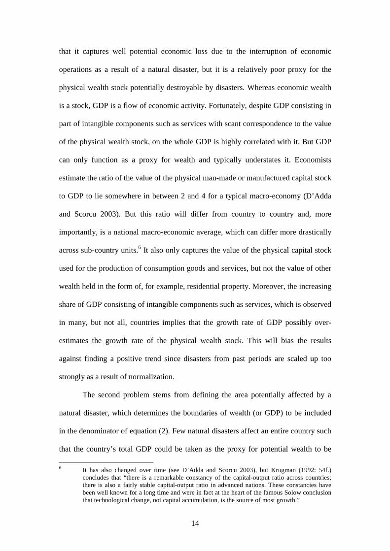
one percent level, is found using the alternative method.15 In contrast, the analysis

yields no significant trends using either method for developing countries (figure 5b).

This could possibly indicate a stronger capability of richer nations to fund defensive

15 Interestingly, while hurricane Katrina is the major reason for conventionally normalized loss

in 2005 to represent the largest loss in developed countries over the period 1980 to 2009, the sum of APLRs for 2005 is not even in the top three over this period. The reason is that while Katrina caused a very large economic loss, it also hit a relatively wealthy part of the developed world.

22

mitigating measures, which decrease vulnerability to natural disasters over time. As

shown in figure 5c, the negative and significant trend is prevalent when normalizing

with the alternative method for the US and Canada.16 For all other selected regions,

namely Western Europe (figure 5d), Latin America and the Caribbean (figure 5e), as

well as South and East Asia and Pacific countries (figure 5f), no statistically

significant trend is found under either approach.

Climate change also need not affect all climate-related disasters equally and in

the same way. In figures 6a to 6d we therefore look at specific disaster types at the

global level. For convective events (figure 6a), that is, damages from flash floods, hail

storms, tempest storms, tornados, and lightning, there is no statistically significant

trend, according to either normalization approaches. The same result is found for

storm events (figure 6b) and for tropical cyclones (figure 6c). For precipitation-related

events (figure 6d), we find no trend with the conventional approach, but a negative

trend with the alternative method, which is significant at the ten percent level.

There is concern about specific climate-related disasters affecting specific

regions, which is not sufficiently addressed by any of the analysis reported above. In

figures 7a to 7d, we therefore look at specific disaster events in specific regions or

countries. To begin with, Figure 7a displays disaster losses from convective events in

the US. For the United States, data quality in the NatCat dataset is high also for earlier

years back to 1970. We therefore are able to cover 40 years in this analysis. If losses

are normalized according to the conventional method, a positive and statistically

significant trend can be established. With the alternative method, however, the

positive trend is marginally insignificant (p-value of 0.129). For the same disaster

type in Europe, on the other hand, no significant trend is discernible after

16 The trend remains statistically significant at the five percent level if the large value in the year

1984 is excluded.

23

normalization with either approach (figure 7b). Disaster losses caused by hurricanes

in the US and in the Central American and Caribbean region have been subject to

various focussed studies (Pielke and Landsea 1998, Pielke et al. 2003, Nordhaus

2006, Pielke et al. 2008).17 We do not find a significant trend either in the United

States (figure 7c) or in Central America and the Caribbean (figure 7d), independent of

the normalisation approach applied. At face value, the result for the US contradicts

studies, which have found an upward trend in US hurricane losses since the 1970s

(e.g,, Schmidt, Kemfert and Höppe 2009). Note, however, that the trend with the

conventional normalization approach is not too far from statistical significance (p-

value of 0.166).18

6. Defensive mitigating measures

One of the problems with normalizing damage from natural disasters, independently

of the method chosen, is our inability to take into account defensive mitigating

measures, which rational individuals would undertake in response to an increasing

frequency and/or intensity of natural hazards. An increase in such measures could

prevent an increasing trend in natural disaster loss that would otherwise occur in the

absence of such measures and could thus prevent detection of a potential climate

change signal in the data. For example, flood defence measures in Western Europe

have dramatically reduced the risk of flood damages from winter storms (e.g., Lavery

and Donovan (2005) on the River Thames tidal defences or Ronde et al. (2003) on

flood defence development in the Netherlands), while stricter building codes

introduced in parts of coastal Florida from the mid-1990s onwards have significantly

17 Nordhaus (2006) finds a positive and significant trend in normalised tropical cyclone losses in

the United States. 18 Moreover, if we restrict our analysis to the exact same time period as Schmidt, Kemfert and

Höppe (2009) and regress, as they do, the log of normalized loss (rather than loss itself) on years, then we also find a significant trend.

24

reduced hurricane damage from Hurricane Charley in 2004 (Institute for Business and

Home Safety 2008). Our findings of a downward trend in natural disaster loss with

the alternative method for all natural disasters and for all non-geophysical disasters at

the global level could be driven by such measures. Splitting up the sample into

developed versus developing countries, we find a strong and more clearly statistically

significant downward trend for developed countries, but no trend whatsoever for

developing countries. This would also be consistent with increased defensive

mitigating measures since developed countries are much better able to fund such

measures than developing countries. To be sure, increased mitigating measures are

only one possible explanation for the findings, but not the only one.

With the possible exception of Crompton and McAneney (2008) who study

one specific type of natural disaster in one single country, due to lack of data no

existing study has been able to adequately take defensive mitigating measures into

account, and neither can we. Instead, we offer evidence on trends in the frequency of

natural disasters, which could tentatively point in the direction that such measures are

increasingly undertaken. To this effect, figure 8 shows trends in the simple count of

disasters, once for weather-related and once for geophysical disasters not related to

weather. There seems to be a clear upward trend in the frequency count of weather-

related disasters. There is also an upward trend in the frequency count of geophysical

disasters. However, the trend line for weather-related disaster counts suggests more

than a doubling over the period 1980 to 2009, whereas the trend line for geophysical

disasters suggests only a small percentage increase over this period. A natural

question is whether this strongly increasing trend in the frequency count of weather-

related disasters is driven by increased awareness and reporting of natural disasters in

later compared to earlier periods as well as by new settlements in areas that were

25

uninhabited before as populations and economies grow and where the same natural

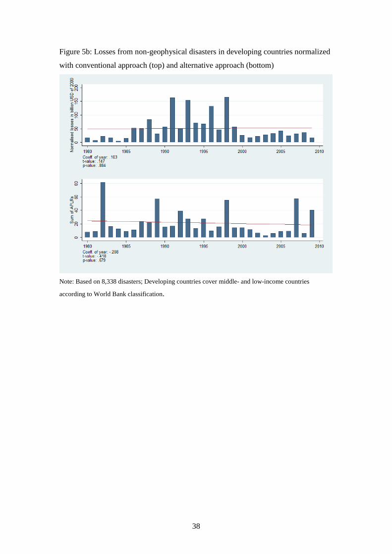
hazard would have gone unrecorded (no damage) before. To check this, in figure 9 we

repeat the exercise from figure 8, but this time restricting the analysis to major

disasters, for which a reporting bias is less likely. Major disasters are defined as

disasters that exceed a property damage value, which is linearly interpolated from 85

million USD in 1980 to 200 million USD in 2009, or exceed a (time-invariant) fatality

level of 100 people killed. As before, there is a clear upward trend in the frequency

count of major weather-related disasters, but there is also an upward trend in the count

of major geophysical disasters. As before, the frequency count of weather-related

disasters increases relatively more than the frequency count of geophysical disasters.

However, since there is no physical reason why the frequency count of major

geophysical disasters should have increased, some reporting bias is likely to remain

present even for major disasters, unless the increase can be fully explained by there

being fewer uninhabited areas available in later periods. It is impossible to say how

large this reporting bias is, but there could well be some increase in the frequency of

weather-related disasters beyond what can be explained by reporting bias.

Interestingly, one observes a similar upward trend in the frequency of weather-related

disasters, both all and major ones only, for a country like Germany, in which

reporting bias is not very likely and where no major expansion of population into

previously unsettled areas has taken place over the period of our study (no figures

shown, but available upon request).

Independently of the reason behind the strong increase in the frequency count

of weather-related disasters over our period of analysis, how can this be reconciled

with our finding of no upward trend in normalized damage from natural disasters?

There are three possibilities. First, there could be an opposite reporting bias in terms

26

of damage caused such that economic loss is over-estimated in the early years of our

study period and under-estimated in the later years. Second, weather-related natural

disasters could have become less intensive over time. Third, weather-related natural

disasters have not become less intensive, but defensive mitigating measures have

prevented increasingly frequent weather-related natural disasters from causing an

upward trend in normalized natural disaster loss. Since there is little reason to

presume that loss has been systematically over-estimated in the past or that weather-

related natural disasters have become less intensive, the third explanation presents a

distinct possibility.

7. Conclusion

In this article, we have analyzed whether one can detect an increasing trend in

historical data on economic damage from natural disasters. We have argued that the

conventional method used for normalization is theoretically problematic as it fails to

normalize for a spatially heterogeneous distribution of wealth which renders absolute

losses from different locations non-comparable to each other. We have proposed an

alternative method, which normalizes disaster loss for both differences in space and

time. The actual-to-potential loss (APLR) ratio provides a theoretically correct and

valid normalization method for economic disaster loss. Contrary to conventional

normalization, our proposed alternative is valid for the purpose of detecting a climate

signal in the sense that it will always attribute a higher value to periods in which,

ceteris paribus, more disasters of the same intensity take place or the same number of

disasters strike with higher intensity. Yet, our theoretically correct measure of disaster

loss encounters many more practical difficulties than the conventional normalization

27

method, particularly if applied at the global level. We have therefore undertaken our

analysis with both methods, regarding them as complements, not substitutes.

Independently of the method used, we find no significant upward trend in

normalized disaster loss. This holds true whether we include all disasters or take out

the ones unlikely to be affected by a changing climate. It also holds true if we step

away from a global analysis and look at specific regions or step away from pooling all

disaster types and look at specific types of disaster instead or combine these two sets

of dis-aggregated analysis.

Much caution is required in correctly interpreting these findings. What the

results tell us is that, based on historical data, there is no evidence so far that climate

change has increased the normalized economic loss from natural disasters. More

cannot be inferred from the data. In particular, one cannot infer from our analysis that

there have not been more frequent and/or more intensive weather-related natural

disasters.19 Our analysis necessarily cannot take into account defensive mitigating

measures undertaken by rational individuals and governments and a serious attempt at

trying to collect data on such measures should top the priority list for future research.

Such measures would translate into lower economic damage compared to the damage

in the absence of defensive mitigation and if mitigating measures have increased and

strengthened over time then this increasing trend toward mitigation could well mask

an increasing trend in natural disaster loss over time. Our finding of an increasing

trend in the frequency count of weather-related disasters, including only major ones,

tentatively points in the direction of an increasing trend toward such defensive

mitigating measures, unless the trend were fully explained by reporting bias. Besides

the issue of defensive mitigating measures, another caveat to keep in mind in making

19 In fact, our frequency count of weather-related natural disasters suggests increasing rather

than decreasing frequency of such disasters.

28

inferences from our analysis is that it is based on historical data. Available evidence

suggests that climatic change has only just begun and that it will take many years and

decades still before its consequences will be truly felt (IPCC 2007a, 2007b). If so, the

past will be a poor guide to the future.

In sum, while we find no evidence for an increasing trend in normalized

economic damage from natural disasters, this provides no reason for complacency.

That inflation-adjusted non-normalized disaster damage is significantly increasing

should prompt policy-makers into seriously considering measures to prevent the

further accumulation of wealth in disaster-prone areas. More importantly for the

debate on climate change, our results do not undermine the argument of those who,

based on the precautionary principle, call for reducing greenhouse gas emissions in

order to prevent or reduce a potentially increasing economic toll from natural disasters

in the future. We find no evidence for an increasing trend in the normalized economic

toll from natural disasters based on historical data, but given our inability to control

for defensive mitigating measures we cannot rule out its existence, let alone rule out

the possibility of an increasing trend in the future.

29

References

Barredo, J.I., 2009, Normalised flood losses in Europe: 1970–2006, Natural Hazards

and Earth Systems Sciences, 9, pp. 97-104.

Bouwer, Laurens M., 2009, Have past disaster losses increased due to anthropogenic

climate change?, Amsterdam: VU University.

Brooks, Harold E. and Charles A. Doswell, 2001, Normalized Damage from Major

Tornados in the United States: 1890-1999, Weather and Forecasting, 16, pp.

168-176.

Crompton, Ryan P. and K. John McAneney, 2008, Normalised Australian insured

losses from meteorological hazards: 1967-2006, Environmental Science &

Policy, pp. 371-378.

D’Adda, Carlo and Antonello E. Scorcu, 2003, On the Time Stability of the Output-

capital Ratio, Economic Modelling, 20, pp. 1175-1189.

De Ronde, J.G., J.P.M. Mulder, and R. Spanhoff, 2003, Morphological Developments

and Coastal Zone Management in the Netherlands, International Conference on

Estuaries and Coasts November 9-11, 2003, Hangzhou, China.

G-Econ, 2010, Geographically based Economic data, http://gecon.yale.edu/, last

accessed: March, 26th 2010.

IPCC, 2001, Climate Change 2001: Impacts, Adaptation, and Vulnerability, New

York: Cambridge University Press.

IPCC, 2007a, Climate Change 2007: The Physical Science Basis, New York:

Cambridge University Press.

IPCC, 2007b, Climate Change 2007: Impacts, Adaptation, and Vulnerability, New

York: Cambridge University Press.

30

Institute for Business and Home Safety, 2008, The Benefits of Modern Wind

Resistant Building Codes on Hurricane Claim Frequency and Severity – A

Summary Report; available at: http://www.ibhs.org/newsroom/downloads

/20070810_102941_10167.pdf.

Katz, R. W., 2002, Stochastic modeling of hurricane damage, Journal of Applied

Meteorology, 41(7), pp. 754-762.

Krugman, Paul, 1992, Comment. NBER Macroeconomics Annual, 7, pp. 54-56.

Lavery, Sarah and Bill Donovan, 2005, Flood risk management in the Thames

Estuary looking ahead 100 years, Philosophical Transactions of the Royal

Society A, 363, pp. 1455-1474.

Miller, Stuart, Robert Muir-Wood and Auguste Boissonade, 2008, An exploration of

trends in normalized weather-related catastrophe losses, in: Diaz, Henry F. and

Richard J. Murnane (eds), Climate Extremes and Society, New York: Cambridge

University Press.

Nordhaus, William D., 2006, The Economics of Hurricanes in the United States,

Working Paper. New Haven: Yale University.

Nordhaus, William, Q. Azam, D. Corderi, K. Hood, N. M. Victor, M, Mohammed, A,

Miltner, and J, Weiss, 2006, The G-Econ Database on Gridded Output: Methods

and Data, New Haven: Yale University.

Pielke, Roger A. Jr., 2007, Mistreatment of the economic impacts of extreme events

in the Stern Review Report on the Economics of Climate Change, Global

Environmental Change, 17, pp. 302-310.

Pielke, Roger A. Jr. and Christopher W. Landsea, 1998, Normalized Hurricane

Damages in the United States: 1925-1995, Weather and Forecasting, Sept. 1998,

pp. 621-631.

31

Pielke, Roger A. Jr., Christopher W. Landsea, Rade T. Musulin and Mary Downton,

1999, Evaluation of Catastrophe Models using a Normalized Historical Record,

Journal of Insurance Regulation, 18(2), pp. 177-194.

Pielke, Roger A. Jr., Jose Rubiera, Christopher Landsea, Mario L. Fernández, and

Roberta Klein, 2003, Hurricane Vulnerability in Latin America and The

Caribbean: Normalized Damages and Loss Potentials, Natural Hazards Review,

4(3), pp. 101-114.

Pielke, R. A., Jr., Gratz, J., Landsea, C. W., Collins, D., Saunders, M. A., and

Musulin, R., 2008, Normalized hurricane damages in the United States: 1900–

2005, Natural Hazards Review, 9(1), pp. 29-42.

Raghavan, S. and S. Rajseh, 2003, Trends in Tropical Cyclone Impact: A Study in

Andhra Pradesh, India, American Meteorological Society, 84, pp. 635-644.

Schmidt, Silvio, Claudia Kemfert and Peter Höppe, 2009, Tropical cyclone losses in

the USA and the impact of climate change — A trend analysis based on data

from a new approach to adjusting storm losses, Environmental Impact

Assessment Review, 29, pp. 359-369.

Schwab, Anna K., Katherine Eschelbach and David J. Brower, 2007, Hazard

Mitigation and Preparedness. Hoboken: Wiley & Sons.

Stern, Nicholas, 2007, The Economics of Climate Change – The Stern Review,

Cambridge: Cambridge University Press.

Vranes, Kevin and Roger Pielke Jr., 2009, Normalized Earthquake Damage and

Fatalities in the United States: 1900-2005, Natural Hazards Review, 10(3), pp.

84-101.

World Bank, 2010, World Development Indicators Online Database. Washington,

DC: World Bank.

32

Figure 1a: Determining the affected area.

Note: Example shows the situation on the Northern hemisphere east of the zero meridian; Dot shows

the geo-reference of disaster centre; different shades represent different levels of GDP.

1° lat

2° lat

3° lat

4° lat

1° long 2° long 3° long 4° long 5° long

33

Figure 1b: Determining the affected area if disaster centre is on the intersection of a

degree of longitude and a degree of latitude

Note: Example shows the situation on the Northern hemisphere east of the zero meridian; Dot shows

the geo-reference of disaster centre; different shades represent different levels of GDP.

1° lat

2° lat

3° lat

4° lat

1° long 2° long 3° long 4° long 5° long

34

Figure 2: Global deflated losses from natural disasters

Note: Based on 20,375 disasters.

35

Figure 3: Global losses from all natural disasters normalized with conventional

approach (top) and alternative approach (bottom)


36

Figure 4: Global losses from non-geophysical disasters normalized with conventional



37

Figure 5a: Losses from non-geophysical disasters in developed countries normalized

with conventional approach (top) and alternative approach (bottom)

Note: Based on 8,307 disasters; developed countries cover OECD countries and other high-income

countries according to World Bank classification.

38

Figure 5b: Losses from non-geophysical disasters in developing countries normalized


Note: Based on 8,338 disasters; Developing countries cover middle- and low-income countries

according to World Bank classification.

39

Figure 5c: Losses from non-geophysical disasters in USA and Canada normalized



40

Figure 5d: Losses from non-geophysical disasters in Western Europe normalized with

conventional approach (top) and alternative approach (bottom)


41

Figure 5e: Losses from non-geophysical disasters in Latin America and The

Caribbean normalized with conventional approach (top) and alternative approach

(bottom)


42

5f: Losses from non-geophysical disasters in South and East Asian and in Pacific

countries normalized with conventional approach (top) and alternative approach

(bottom)


43

Figure 6a: Global disaster losses from convective events normalized with


Note: Based on 5,869 disasters; Includes damages from flash floods, hail storms, tempest storms,

tornados, and lightning.

44

Figure 6b: Global disaster losses from storm events normalized with conventional


Note: Based on 6,179 disasters; Includes damages from winter storms (winter storm and blizzard/ snow storm), convective storms (hail storm, tempest storm, tornado, and lightning), sand storms, local windstorms, and storm surges.

45

Figure 6c: Global disaster losses from tropical cyclones normalized with conventional



46

Figure 6d: Global disaster losses from precipitation-related events normalized with


Note: Based on 6,507 disasters; Includes damages from flooding (flash flood and general flood) and

mass movement (rock falls, landslides, and avalanches).

47

Figure 7a: Disaster losses from convective events in the United States normalized




48

Figure 7b: Disaster losses from convective events in Western Europe normalized with




49

Figure 7c: Disaster losses from hurricanes in the United States normalized with


Note: Based on 118 disasters.

50

Figure 7d: Disaster losses from hurricanes in Central America and The Caribbean

normalized with conventional approach (top) and alternative approach (bottom)

Note: Based on 295 disasters.

51

Figure 8: Annual frequency count of geophysical and weather-related disasters

52

Figure 9: Annual frequency count of major geophysical and weather-related disasters

Documents

Normalizing economic loss from natural disasters - Centre for