Normaliz 3.1

Normaliz 3.1.1

March 31, 2016

Winfried Bruns, Tim Römer, Richard Sieg and Christof Söger

Normaliz 2 team member: Bogdan Ichim

http://normaliz.uos.de

mailto:[email protected]

Contents

1. Introduction 61.1. The objectives of Normaliz . . . . . . . . . . . . . . . . . . . . . . . . . . . 61.2. Platforms, implementation and access from other systems . . . . . . . . . . . 71.3. Major changes relative to version 3.0 . . . . . . . . . . . . . . . . . . . . . . 71.4. Future extensions . . . . . . . . . . . . . . . . . . . . . . . . . . . . . . . . 81.5. Download and installation . . . . . . . . . . . . . . . . . . . . . . . . . . . 8

2. Normaliz by examples 82.1. Terminology . . . . . . . . . . . . . . . . . . . . . . . . . . . . . . . . . . . 82.2. Practical preparations . . . . . . . . . . . . . . . . . . . . . . . . . . . . . . 92.3. A cone in dimension 2 . . . . . . . . . . . . . . . . . . . . . . . . . . . . . 11

2.3.1. The Hilbert basis . . . . . . . . . . . . . . . . . . . . . . . . . . . . 112.3.2. The cone by inequalities . . . . . . . . . . . . . . . . . . . . . . . . 132.3.3. The interior . . . . . . . . . . . . . . . . . . . . . . . . . . . . . . . 13

2.4. A lattice polytope . . . . . . . . . . . . . . . . . . . . . . . . . . . . . . . . 162.4.1. Only the lattice points . . . . . . . . . . . . . . . . . . . . . . . . . 18

2.5. A rational polytope . . . . . . . . . . . . . . . . . . . . . . . . . . . . . . . 182.5.1. The rational polytope by inequalities . . . . . . . . . . . . . . . . . . 21

2.6. Magic squares . . . . . . . . . . . . . . . . . . . . . . . . . . . . . . . . . . 222.6.1. With even corners . . . . . . . . . . . . . . . . . . . . . . . . . . . 252.6.2. The lattice as input . . . . . . . . . . . . . . . . . . . . . . . . . . . 27

2.7. Decomposition in a numerical semigroup . . . . . . . . . . . . . . . . . . . 28

1


mailto:[email protected]

2.8. A job for the dual algorithm . . . . . . . . . . . . . . . . . . . . . . . . . . 292.9. A dull polyhedron . . . . . . . . . . . . . . . . . . . . . . . . . . . . . . . . 29

2.9.1. Defining it by generators . . . . . . . . . . . . . . . . . . . . . . . . 312.10. The Condorcet paradoxon . . . . . . . . . . . . . . . . . . . . . . . . . . . . 32

2.10.1. Excluding ties . . . . . . . . . . . . . . . . . . . . . . . . . . . . . 332.10.2. At least one vote for every preference order . . . . . . . . . . . . . . 34

2.11. Testing normality . . . . . . . . . . . . . . . . . . . . . . . . . . . . . . . . 352.11.1. Computing just a witness . . . . . . . . . . . . . . . . . . . . . . . . 36

2.12. Inhomogeneous congruences . . . . . . . . . . . . . . . . . . . . . . . . . . 372.12.1. Lattice and offset . . . . . . . . . . . . . . . . . . . . . . . . . . . . 382.12.2. Variation of the signs . . . . . . . . . . . . . . . . . . . . . . . . . . 38

2.13. Integral closure and Rees algebra of a monomial ideal . . . . . . . . . . . . . 392.13.1. Only the integral closure . . . . . . . . . . . . . . . . . . . . . . . . 40

2.14. Only the convex hull . . . . . . . . . . . . . . . . . . . . . . . . . . . . . . 402.15. The integer hull . . . . . . . . . . . . . . . . . . . . . . . . . . . . . . . . . 412.16. Starting from a binomial ideal . . . . . . . . . . . . . . . . . . . . . . . . . 43

3. The input file 453.1. Input items . . . . . . . . . . . . . . . . . . . . . . . . . . . . . . . . . . . 46

3.1.1. The ambient space and lattice . . . . . . . . . . . . . . . . . . . . . 463.1.2. Plain vectors . . . . . . . . . . . . . . . . . . . . . . . . . . . . . . 463.1.3. Formatted vectors . . . . . . . . . . . . . . . . . . . . . . . . . . . . 473.1.4. Plain matrices . . . . . . . . . . . . . . . . . . . . . . . . . . . . . . 473.1.5. Formatted matrices . . . . . . . . . . . . . . . . . . . . . . . . . . . 483.1.6. Constraints in generic format . . . . . . . . . . . . . . . . . . . . . . 483.1.7. Computation goals and algorithmic variants . . . . . . . . . . . . . . 493.1.8. Comments . . . . . . . . . . . . . . . . . . . . . . . . . . . . . . . 493.1.9. Restrictions . . . . . . . . . . . . . . . . . . . . . . . . . . . . . . . 493.1.10. Default values . . . . . . . . . . . . . . . . . . . . . . . . . . . . . 503.1.11. Normaliz takes intersections (almost always) . . . . . . . . . . . . . 50

3.2. Homogeneous generators . . . . . . . . . . . . . . . . . . . . . . . . . . . . 503.2.1. Cones . . . . . . . . . . . . . . . . . . . . . . . . . . . . . . . . . . 503.2.2. Lattices . . . . . . . . . . . . . . . . . . . . . . . . . . . . . . . . . 51

3.3. Homogeneous Constraints . . . . . . . . . . . . . . . . . . . . . . . . . . . 513.3.1. Cones . . . . . . . . . . . . . . . . . . . . . . . . . . . . . . . . . . 513.3.2. Lattices . . . . . . . . . . . . . . . . . . . . . . . . . . . . . . . . . 52

3.4. Inhomogeneous generators . . . . . . . . . . . . . . . . . . . . . . . . . . . 523.4.1. Polyhedra . . . . . . . . . . . . . . . . . . . . . . . . . . . . . . . . 523.4.2. Lattices . . . . . . . . . . . . . . . . . . . . . . . . . . . . . . . . . 52

3.5. Inhomogeneous constraints . . . . . . . . . . . . . . . . . . . . . . . . . . . 523.5.1. Cones . . . . . . . . . . . . . . . . . . . . . . . . . . . . . . . . . . 523.5.2. Lattices . . . . . . . . . . . . . . . . . . . . . . . . . . . . . . . . . 53

2

3.6. Generic constraints . . . . . . . . . . . . . . . . . . . . . . . . . . . . . . . 533.6.1. Forced homogeneity . . . . . . . . . . . . . . . . . . . . . . . . . . 54

3.7. Relations . . . . . . . . . . . . . . . . . . . . . . . . . . . . . . . . . . . . 543.8. Unit vectors . . . . . . . . . . . . . . . . . . . . . . . . . . . . . . . . . . . 553.9. Grading . . . . . . . . . . . . . . . . . . . . . . . . . . . . . . . . . . . . . 55

3.9.1. lattice_ideal . . . . . . . . . . . . . . . . . . . . . . . . . . . . . 553.10. Dehomogenization . . . . . . . . . . . . . . . . . . . . . . . . . . . . . . . 563.11. Pointedness . . . . . . . . . . . . . . . . . . . . . . . . . . . . . . . . . . . 563.12. The zero cone . . . . . . . . . . . . . . . . . . . . . . . . . . . . . . . . . . 563.13. Additional input file for NmzIntegrate . . . . . . . . . . . . . . . . . . . . . 56

4. Computation goals and algorithmic variants 574.1. Default choices and basic rules . . . . . . . . . . . . . . . . . . . . . . . . . 574.2. Computation goals . . . . . . . . . . . . . . . . . . . . . . . . . . . . . . . 58

4.2.1. Lattice data . . . . . . . . . . . . . . . . . . . . . . . . . . . . . . . 584.2.2. Support hyperplanes and extreme rays . . . . . . . . . . . . . . . . . 584.2.3. Hilbert basis and related data . . . . . . . . . . . . . . . . . . . . . . 584.2.4. Enumerative data . . . . . . . . . . . . . . . . . . . . . . . . . . . . 584.2.5. Combined computation goals . . . . . . . . . . . . . . . . . . . . . 584.2.6. The class group . . . . . . . . . . . . . . . . . . . . . . . . . . . . . 594.2.7. Integer hull . . . . . . . . . . . . . . . . . . . . . . . . . . . . . . . 594.2.8. Triangulation and Stanley decomposition . . . . . . . . . . . . . . . 594.2.9. NmzIntegrate . . . . . . . . . . . . . . . . . . . . . . . . . . . . . . 594.2.10. Boolean valued computation goals . . . . . . . . . . . . . . . . . . . 59

4.3. Algorithmic variants . . . . . . . . . . . . . . . . . . . . . . . . . . . . . . 604.4. Integer type . . . . . . . . . . . . . . . . . . . . . . . . . . . . . . . . . . . 604.5. Control of computations . . . . . . . . . . . . . . . . . . . . . . . . . . . . 614.6. Rational and integer solutions in the inhomogeneous case . . . . . . . . . . . 61

5. Running Normaliz 625.1. Basic rules . . . . . . . . . . . . . . . . . . . . . . . . . . . . . . . . . . . . 635.2. Info about Normaliz . . . . . . . . . . . . . . . . . . . . . . . . . . . . . . . 635.3. Control of execution . . . . . . . . . . . . . . . . . . . . . . . . . . . . . . 635.4. Control of output files . . . . . . . . . . . . . . . . . . . . . . . . . . . . . . 645.5. Overriding the options in the input file . . . . . . . . . . . . . . . . . . . . . 64

6. More examples 646.1. Lattice points by approximation . . . . . . . . . . . . . . . . . . . . . . . . 646.2. The bottom decomposition . . . . . . . . . . . . . . . . . . . . . . . . . . . 666.3. Subdivision of large simplicial cones . . . . . . . . . . . . . . . . . . . . . . 676.4. Primal vs. dual – division of labor . . . . . . . . . . . . . . . . . . . . . . . 686.5. Explicit dehomogenization . . . . . . . . . . . . . . . . . . . . . . . . . . . 68

3

6.6. Nonpointed cones . . . . . . . . . . . . . . . . . . . . . . . . . . . . . . . . 706.6.1. A nonpointed cone . . . . . . . . . . . . . . . . . . . . . . . . . . . 706.6.2. A polyhedron without vertices . . . . . . . . . . . . . . . . . . . . . 726.6.3. Checking pointedness first . . . . . . . . . . . . . . . . . . . . . . . 736.6.4. Input of a subspace . . . . . . . . . . . . . . . . . . . . . . . . . . . 736.6.5. Data relative to the original monoid . . . . . . . . . . . . . . . . . . 74

6.7. Exporting the triangulation . . . . . . . . . . . . . . . . . . . . . . . . . . . 756.7.1. Nested triangulations . . . . . . . . . . . . . . . . . . . . . . . . . . 766.7.2. Disjoint decomposition . . . . . . . . . . . . . . . . . . . . . . . . . 77

6.8. Exporting the Stanley decomposition . . . . . . . . . . . . . . . . . . . . . . 786.9. Module generators over the original monoid . . . . . . . . . . . . . . . . . . 79

6.9.1. An inhomogeneous example . . . . . . . . . . . . . . . . . . . . . . 806.10. Precomputed support hyperplanes . . . . . . . . . . . . . . . . . . . . . . . 816.11. Shift, denominator, quasipolynomial and multiplicity . . . . . . . . . . . . . 826.12. A very large computation . . . . . . . . . . . . . . . . . . . . . . . . . . . . 84

7. Optional output files 857.1. The homogeneous case . . . . . . . . . . . . . . . . . . . . . . . . . . . . . 857.2. Modifications in the inhomogeneous case . . . . . . . . . . . . . . . . . . . 86

8. Performance 868.1. Parallelization . . . . . . . . . . . . . . . . . . . . . . . . . . . . . . . . . . 878.2. Running large computations . . . . . . . . . . . . . . . . . . . . . . . . . . 87

9. Distribution and installation 88

10.Compilation 8910.1. General . . . . . . . . . . . . . . . . . . . . . . . . . . . . . . . . . . . . . 8910.2. Linux . . . . . . . . . . . . . . . . . . . . . . . . . . . . . . . . . . . . . . 9010.3. Mac OS X . . . . . . . . . . . . . . . . . . . . . . . . . . . . . . . . . . . . 9010.4. Windows . . . . . . . . . . . . . . . . . . . . . . . . . . . . . . . . . . . . 90

11.Copyright and how to cite 91

A. Mathematical background and terminology 92A.1. Polyhedra, polytopes and cones . . . . . . . . . . . . . . . . . . . . . . . . . 92A.2. Cones . . . . . . . . . . . . . . . . . . . . . . . . . . . . . . . . . . . . . . 93A.3. Polyhedra . . . . . . . . . . . . . . . . . . . . . . . . . . . . . . . . . . . . 93A.4. Affine monoids . . . . . . . . . . . . . . . . . . . . . . . . . . . . . . . . . 95A.5. Affine monoids from binomial ideals . . . . . . . . . . . . . . . . . . . . . . 96A.6. Lattice points in polyhedra . . . . . . . . . . . . . . . . . . . . . . . . . . . 96A.7. Hilbert series . . . . . . . . . . . . . . . . . . . . . . . . . . . . . . . . . . 97A.8. The class group . . . . . . . . . . . . . . . . . . . . . . . . . . . . . . . . . 99

4

B. Annotated console output 99B.1. Primal mode . . . . . . . . . . . . . . . . . . . . . . . . . . . . . . . . . . . 99B.2. Dual mode . . . . . . . . . . . . . . . . . . . . . . . . . . . . . . . . . . . . 101

C. Normaliz 2 input syntax 103

D. libnormaliz 104D.1. Integer type as a template parameter . . . . . . . . . . . . . . . . . . . . . . 104

D.1.1. Alternative integer types . . . . . . . . . . . . . . . . . . . . . . . . 104D.2. Construction of a cone . . . . . . . . . . . . . . . . . . . . . . . . . . . . . 105D.3. Computations in a cone . . . . . . . . . . . . . . . . . . . . . . . . . . . . . 107D.4. Retrieving results . . . . . . . . . . . . . . . . . . . . . . . . . . . . . . . . 109

D.4.1. Checking computations . . . . . . . . . . . . . . . . . . . . . . . . . 109D.4.2. Rank, index and dimension . . . . . . . . . . . . . . . . . . . . . . . 109D.4.3. Support hyperplanes and constraints . . . . . . . . . . . . . . . . . . 110D.4.4. Extreme rays and vertices . . . . . . . . . . . . . . . . . . . . . . . 110D.4.5. Generators . . . . . . . . . . . . . . . . . . . . . . . . . . . . . . . 110D.4.6. Lattice points in polytopes and elements of degree 1 . . . . . . . . . 110D.4.7. Hilbert basis . . . . . . . . . . . . . . . . . . . . . . . . . . . . . . 111D.4.8. Module generators over original monoid . . . . . . . . . . . . . . . . 111D.4.9. Grading and dehomogenization . . . . . . . . . . . . . . . . . . . . 111D.4.10. Enumerative data . . . . . . . . . . . . . . . . . . . . . . . . . . . . 111D.4.11. Triangulation and disjoint decomposition . . . . . . . . . . . . . . . 112D.4.12. Stanley decomposition . . . . . . . . . . . . . . . . . . . . . . . . . 113D.4.13. Coordinate transformation . . . . . . . . . . . . . . . . . . . . . . . 113D.4.14. Class group . . . . . . . . . . . . . . . . . . . . . . . . . . . . . . . 114D.4.15. Integer hull . . . . . . . . . . . . . . . . . . . . . . . . . . . . . . . 114D.4.16. Excluded faces . . . . . . . . . . . . . . . . . . . . . . . . . . . . . 114D.4.17. Boolean valued results . . . . . . . . . . . . . . . . . . . . . . . . . 115

D.5. Exception handling . . . . . . . . . . . . . . . . . . . . . . . . . . . . . . . 116D.6. Control of output . . . . . . . . . . . . . . . . . . . . . . . . . . . . . . . . 116D.7. A simple program . . . . . . . . . . . . . . . . . . . . . . . . . . . . . . . . 117

5

1. Introduction

1.1. The objectives of Normaliz

The program Normaliz is a tool for computing the Hilbert bases and enumerative data of ratio-nal cones and, more generally, sets of lattice points in rational polyhedra. The mathematicalbackground and the terminology of this manual are explained in Appendix A. For a thoroughtreatment of the mathematics involved we refer the reader to [4] and [6]. The terminologyfollows [4]. For algorithms of Normaliz see [5], [7], [8] and [9]. Some new developments arebriefly explained in this manual.

Both polyhedra and lattices can be given by

(1) systems of generators and/or(2) constraints.

Since version 3.1, cones need not be pointed and polyhedra need not have vertices, but areallowed tom contain a positive-dimensional affine subspace.

In addition to generators and constraints, affine monoids can be defined by lattice ideals, inother words, by binomial equations.

In order to define a rational polyhedron by generators, one specifies a finite set of verticesx1, . . . ,xn ∈Qd and a set y1, . . . ,ym ∈ Zd generating a rational cone C. The polyhedron definedby these generators is

P = conv(x1, . . . ,xn)+C, C = R+y1 + · · ·+R+ym.

An affine lattice defined by generators is a subset of Zd given as

L = w+L0, L0 = Zz1 + · · ·+Zzr, w,z1, . . . ,zr ∈ Zd.

Constraints defining a polyhedron are affine-linear inequalities with integral coefficients, andthe constraints for an affine lattice are affine-linear diophantine equations and congruences.The conversion between generators and constraints is an important task of Normaliz.

The first main goal of Normaliz is to compute a system of generators for

P∩L.

The minimal system of generators of the monoid M =C∩L0 is the Hilbert basis Hilb(M) ofM. The homogeneous case, in which P = C and L = L0, is undoubtedly the most importantone, and in this case Hilb(M) is the system of generators to be computed. In the general casethe system of generators consists of Hilb(M) and finitely many points u1, . . . ,us ∈ P∩L suchthat

P∩L =s⋃

j=1

u j +M.

The second main goal are enumerative data that depend on a grading of the ambient lattice.Normaliz computes the Hilbert series and the Hilbert quasipolynomial of the monoid or set

6

of lattice points in a polyhedron. In combinatorial terminology: Normaliz computes Ehrhartseries and quasipolynomials of rational polyhedra. Via its offspring NmzIntegrate [11], Nor-maliz computes generalized Ehrhart series and Lebesgue integrals of polynomials over rationalpolytopes.

The computation goals of Normaliz can be set by the user. In particular, they can be restrictedto subtasks, such as the lattice points in a polytope or the leading coefficient of the Hilbert(quasi)polynomial.

Performance data of Normaliz can be found in [8].

Acknowledgement. The development of Normaliz is currently supported by the DFG SPP1489 “Algorithmische und experimentelle Methoden in Algebra, Geometrie und Zahlentheo-rie”.

1.2. Platforms, implementation and access from other systems

Executables for Normaliz are provided for Mac OS, Linux and MS Windows. If the executa-bles prepared cannot be run on your system, then you can compile Normaliz yourself (seeSection 10).

Normaliz is written in C++, and should be compilable on every system that has a GCC com-patible compiler. It uses the standard packages Boost and GMP (see Section 10). The paral-lelization is based on OpenMP.

The executables provided by us use the integer optimization program SCIP [1] for certainsubtasks, but the inclusion of SCIP must be activated at compile time.

Normaliz consists of two parts: the front end normaliz for input and output and the C++ librarylibnormaliz that does the computations.

Normaliz can be accessed from the following systems:

• SINGULAR via the library normaliz.lib,• MACAULAY 2 via the package Normaliz.m2,• COCOA via an external library and libnormaliz,• GAP via the GAP package NORMALIZINTERFACE [12] which uses libnormaliz,• POLYMAKE (thanks to the POLYMAKE team),• SAGE via an optional package by A. Novoseltsev.

The Singular and Macaulay 2 interfaces are contained in the Normaliz distribution. At present,their functionality is limited to Normaliz 2.10.

Furthermore, Normaliz is used by the B. Burton’s system REGINA.

Normaliz does not have its own interactive shell. We recommend the access via GAP forinteractive use.

1.3. Major changes relative to version 3.0

(1) Normaliz computes nonpointed cones and polyhedra without vertices.

7

(2) Rational and integral solutions of inhomogeneous systems can be separated.(3) Integer hull computation.(4) Normality test without computation of full Hilbert basis (in the negative case).(5) Normaliz can be run from the beginning with integers of type long long.(6) Computation of disjoint decomposition of the cone.

For version 3.1.1 we have added

(1) Input of generic constraints,(2) input of formatted vectors and matrices,(3) input of transposed matrices.

1.4. Future extensions

(1) Exploitation of symmetries.(2) Access from further systems.(3) Gröbner and Graver bases.

1.5. Download and installation

Download

• the zip file with the Normaliz source, documentation, examples and further platformindependent components, and• the zip file containing the executable(s) for your system

from the Normaliz website


and unzip both in the same directory of your choice. In it, a directory Normaliz3.0 (calledNormaliz directory in the following) is created with several subdirectories.

See Section 9 for more details on the distribution and consult Section 10 if you want to compileNormaliz yourself.

2. Normaliz by examples

2.1. Terminology

For the precise interpretation of parts of the Normaliz output some terminology is necessary,but this section can be skipped at first reading, and the user can come back to it when itbecomes necessary. We will give less formal descriptions along the way.

As pointed out in the introduction, Normaliz “computes” intersections P∩ L where P is arational polyhedron in Rd and L is an affine sublattice of Zd . It proceeds as follows:

8


(1) If the input is inhomogeneous, then it is homogenized by introducing a homogenizingcoordinate: the polyhedron P is replaced by the cone C(P): it is the closure of R+(P×{1} in Rd+1. Similarly L is replaced by L = Z(L×{1}). In the homogeneous case inwhich P is a cone and L is a subgroup of Zd , we set C(P) = P and L = L.

(2) The computations take place in the efficient lattice

E= L∩RC(P).

where RC(P) is the linear subspace generated by C(P). The internal coordinates arechosen with respect to a basis of E. The efficient cone is

C= R+(C(P)∩E).

(3) Inhomogeneous computations are truncated using the dehomogenization (defined im-plicitly or explicitly).

(4) The final step is the conversion to the original coordinates. Note that we must use thecoordinates of Rd+1 if homogenization has been necessary, simply because some outputvectors may be non-integral.

Normaliz computes inequalities, equations and congruences defining E and C. The outputcontains only those constraints that are really needed. They must always be used jointly: theequations and congruences define E, and the equations and inequalities define C. Altogetherthey define the monoid M = C∩E. In the homogeneous case this is the monoid to be com-puted. In the inhomogeneous case we must intersect M with the dehomogenizing hyperplaneto obtain P∩L.

In this section, only pointed cones (and polyhedra with vertices) will be discussed. Nonpointedcones will be addressed in Section 6.6.

2.2. Practical preparations

You may find it comfortable to run Normaliz via the GUI jNormaliz [2]. In the Normalizdirectory open jNormaliz by clicking jNormaliz.jar in the appropriate way. (We assume thatJava is installed on your machine.) In the jNormaliz file dialogue choose one of the input filesin the subdirectory example, say small.in, and press Run. In the console window you canwatch Normaliz at work. Finally inspect the output window for the results.

The menus and dialogues of jNormaliz are self explanatory, but you can also consult thedocumentation [2] via the help menu.

Moreover, one can, and often will, run Normaliz from the command line. This is fully ex-plained in Section 5. At this point it is enough to call Normaliz by typing

normaliz -c <project>

where <project> denotes for the project to be computed. Normaliz will load the file project.in.The option -c makes Normaliz to write a progress report on the terminal. Normaliz writes itsresults to <project>.out.

9

Figure 1: jNormaliz

Note that you may have to prefix normaliz by a path name, and <project> must contain apath to the input file if it is not in the current directory. Suppose the Normaliz directory is thecurrent directory and we are using a Linux or Mac system. Then

./normaliz -c example/small

will run small.in from the directory example. On Windows we must change this to

.\normaliz -c example\small

The commands given above will run Normaliz with the full parallelization that your systemcan deliver. For the very small examples in this tutorial you may want to add -x=1 to suppressparallelization.

As long as you don’t specify a computation goal on the command line or in the input file,Normaliz will use the default computation goals:

HilbertBasis

HilbertSeries

ClassGroup

The computation of the Hilbert series requires the explicit or implicit definition of a grading.Normaliz does only complain that a computation goal cannot be reached if the goal has beenset explicitly. For example, if you say HilbertSeries and there is no grading, an exceptionwill be thrown and Normaliz terminates, but an output file with the already computed data willbe written.

Normaliz will always print the results that are obtained on the way to the computation goalsand do not require extra effort.

Appendix B helps you to read the console output that you have demanded by the option -c.

10

2.3. A cone in dimension 2

We want to investigate the cone C = R+(2,1)+R+(1,3)⊂ R2:

0

This cone is defined in the input file 2cone.in:

amb_space 2

cone 2

1 3

2 1

The input tells Normaliz that the ambient space is R2, and then a cone with 2 generators isdefined, namely the cone C from above.

The figure indicates the Hilbert basis, and this is our first computation goal.

If you prefer to consider the columns of a matrix as input vectors (or have got a matrix in thisformat from another system) you can use the input

amb_space 2

cone transpose 2

1 2

3 1

Note that the 2 following transpose is now the number of columns. Later on we will alsoshow the use of formatted matrices.

2.3.1. The Hilbert basis

In order to compute the Hilbert basis, we run Normaliz from jNormaliz or by

./normaliz -c example/2cone

and inspect the output file:

4 Hilbert basis elements

2 extreme rays

2 support hyperplanes

Self explanatory so far.

11

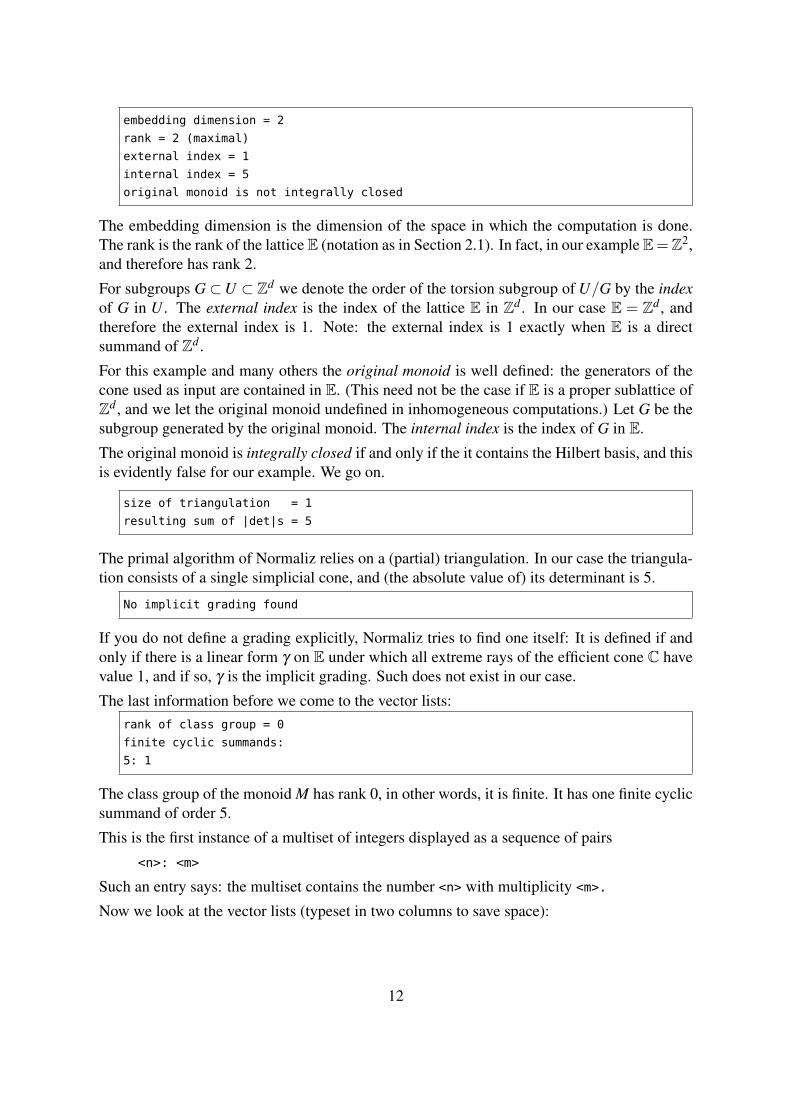
embedding dimension = 2

rank = 2 (maximal)

external index = 1

internal index = 5

original monoid is not integrally closed

The embedding dimension is the dimension of the space in which the computation is done.The rank is the rank of the lattice E (notation as in Section 2.1). In fact, in our example E=Z2,and therefore has rank 2.

For subgroups G⊂U ⊂ Zd we denote the order of the torsion subgroup of U/G by the indexof G in U . The external index is the index of the lattice E in Zd . In our case E = Zd , andtherefore the external index is 1. Note: the external index is 1 exactly when E is a directsummand of Zd .

For this example and many others the original monoid is well defined: the generators of thecone used as input are contained in E. (This need not be the case if E is a proper sublattice ofZd , and we let the original monoid undefined in inhomogeneous computations.) Let G be thesubgroup generated by the original monoid. The internal index is the index of G in E.

The original monoid is integrally closed if and only if the it contains the Hilbert basis, and thisis evidently false for our example. We go on.

size of triangulation = 1

resulting sum of |det|s = 5

The primal algorithm of Normaliz relies on a (partial) triangulation. In our case the triangula-tion consists of a single simplicial cone, and (the absolute value of) its determinant is 5.

No implicit grading found

If you do not define a grading explicitly, Normaliz tries to find one itself: It is defined if andonly if there is a linear form γ on E under which all extreme rays of the efficient cone C havevalue 1, and if so, γ is the implicit grading. Such does not exist in our case.

The last information before we come to the vector lists:rank of class group = 0

finite cyclic summands:

5: 1

The class group of the monoid M has rank 0, in other words, it is finite. It has one finite cyclicsummand of order 5.

This is the first instance of a multiset of integers displayed as a sequence of pairs

<n>: <m>

Such an entry says: the multiset contains the number <n> with multiplicity <m>.

Now we look at the vector lists (typeset in two columns to save space):

12

4 Hilbert basis elements: 2 extreme rays:

1 1 1 3

1 2 2 1

1 3

2 1 2 support hyperplanes:

-1 2

3 -1

The support hyperplanes are given by the linear forms (or inner normal vectors):

−x1 +2x2 ≥ 0,3x1− x2 ≥ 0.

If the order is not fixed for some reason, Normaliz sorts vector lists as follows : (1) by degreeif a grading exists and the application makes sense, (2) lexicographically.

2.3.2. The cone by inequalities

Instead by generators, we can define the cone by the inequalities just computed (2cone_ineq.in).We use this example to show the input of a formamtted matrix:

amb_space auto

inequalities

[[-1 2] [3 -1]]

A matrix of input type inequalities contains homogeneous inequalities. Normaliz can deter-mine the dimension of the ambient space from the formatted matrix. Therefore we can declarethe ambient space as being “auto determined” (but amb_space 2 is not forbidden).

We get the same result as with 2cone.in except that the data depending on the original monoidcannot be computed: the internal index and the information on the original monoid are missingsince there is no original monoid.

2.3.3. The interior

Now we want to compute the lattice points in the interior of our cone. If the cone C is givenby the inequalities λi(x) ≥ 0 (within aff(C)), then the interior is given by the inequalitiesλi(x)> 0. Since we are interested in lattice points, we work with the inequalities λi(x)≥ 1.

The input file 2cone_int.in says

amb_space 2

strict_inequalities 2

-1 2

3 -1

13

The strict inequalities encode the conditions

−x1 +2x2 ≥ 1,3x1− x2 ≥ 1.

This is our first example of inhomogeneous input.

0

Alternatively we could use the following two equivalent input files, in a more intuitive nota-tion:

amb_space 2

constraints 2

-1 2 > 0

3 -1 > 0

amb_space 2

constraints 2

-1 2 >= 1

3 -1 >= 1

Normaliz homogenizes inhomogeneous computations by introducing an auxiliary homogeniz-ing coordinate xd+1. The polyhedron is obtained by intersecting the homogenized cone withthe hyperplane xd+1 = 1. The recession cone is the intersection with the hyperplane xd+1 = 0.The recession monoid is the monoid of lattice points in the recession cone, and the set of latticepoints in the polyhedron is represented by its system of module generators over the recessionmonoid.

Note that the homogenizing coordinate serves as the denominator for rational vectors. In ourexample the recession cone is our old friend that we have already computed, and therefore weneed not comment on it.

2 module generators

4 Hilbert basis elements of recession monoid

1 vertices of polyhedron

2 extreme rays of recession cone

2 support hyperplanes of polyhedron

14


affine dimension of the polyhedron = 2 (maximal)

rank of recession monoid = 2

The only surprise may be the embedding dimension: Normaliz always takes the dimensionof the space in which the computation is done. It is the number of components of the outputvectors. Because of the homogenization it has increased by 1.



In this case the homogenized cone has stayed simplicial, but the determinant has changed.

dehomogenization:

0 0 1

The dehomogenization is the linear form δ on the homogenized space that defines the hyper-planes from which we get the polyhedron and the recession cone by the equations δ (x) = 1and δ (x) = 0, respectively. It is listed since one can also work with a user defined dehomoge-nization.

module rank = 1

This is the rank of the module of lattice points in the polyhedron over the recession monoid.In our case the module is an ideal, and so the rank is 1.

The output of inhomogeneous computations is always given in homogenized form. The lastcoordinate is the value of the dehomogenization on the listed vectors, 1 on the module gener-ators, 0 on the vectors in the recession monoid:

2 module generators: 4 Hilbert basis elements of recession monoid:

1 1 1 1 1 0

1 2 1 1 2 0

1 3 0

2 1 0

The module generators are (1,1) and (1,2).

1 vertices of polyhedron:

3 4 5

Indeed, the polyhedron has a single vertex, namely (3/5,4/5).

2 extreme rays of recession cone: 2 support hyperplanes of polyhedron:

1 3 0 -1 2 -1

2 1 0 3 -1 -1

The support hyperplanes are exactly those that we have used to define the polyhedron. This isobvious in our example, but need not always be true since one or more of the defining inputhyperplanes may be superfluous.

15

2.4. A lattice polytope

The file polytope.in contains

amb_space 4

polytope 4

0 0 0

2 0 0

0 3 0

0 0 5

The Ehrhart monoid of the integral polytope with the 4 vertices

(0,0,0) , (2,0,0) , (0,3,0) and (0,0,5)

in R3 is to be computed. The generators of the Ehrhart monoid are obtained by attaching afurther coordinate 1 to the vertices, and this explains amb_space 4. In fact, the input typepolytope is nothing but a convenient (perhaps superfluous) version of

amb_space 4

cone 4

0 0 0 1

2 0 0 1

0 3 0 1

0 0 5 1

Running normaliz produces the file polytope.out:


18 Hilbert basis elements of degree 1

4 extreme rays



rank = 4 (maximal)

external index = 1

internal index = 30


Perhaps a surprise: the lattice points of the polytope do not yield all Hilbert basis elements.



Nothing really new so far. But now Normaliz finds a grading given by the last coordinate. See3.9 below for general information on gradings.

grading:

0 0 0 1

16

degrees of extreme rays:

1: 4

Again we encounter the notation <n>: <m>: we have 4 extreme rays, all of degree 1.

Hilbert basis elements are not of degree 1

Perhaps a surprise: the polytope is not integrally closed as defined in [4]. Now we see theenumerative data defined by the grading:

multiplicity = 30

Hilbert series:

1 14 15

denominator with 4 factors:

1: 4

degree of Hilbert Series as rational function = -2

Hilbert polynomial:

1 4 8 5

with common denominator = 1

The polytope has Z3-normalized volume 30 as indicated by the multiplicity. The Hilbert(or Ehrhart) function counts the lattice points in kP, k ∈ Z+. The corresponding generatingfunction is a rational function H(t). For our polytope it is

1+14t +15t2

(1− t)4 .

The denominator is given in multiset notation: 1: 4 say that the factor (1− t1) occurs withmultiplicity 4.

The Ehrhart polynomial (again we use a more general term in the output file) of the polytopeis

p(k) = 1+4k+8k2 +5k3 .

In our case it has integral coefficients, a rare exception. Therefore one usually needs a denom-inator.

Everything that follows has already been explained.

rank of class group = 0


30: 1

***********************************************************************

17

18 Hilbert basis elements of degree 1:

0 0 0 1

...

2 0 0 1

1 further Hilbert basis elements of higher degree:

1 2 4 2

4 extreme rays: 4 support hyperplanes:

0 0 0 1 -15 -10 -6 30

0 0 5 1 0 0 1 0

0 3 0 1 0 1 0 0

2 0 0 1 1 0 0 0

The support hyperplanes give us a description of the polytope by inequalities: it is the solutionof the system of the 4 inequalities

x3 ≥ 0 , x2 ≥ 0 , x1 ≥ 0 and 15x1 +10x2 +6x3 ≤ 30 .

2.4.1. Only the lattice points

Suppose we want to compute only the lattice points in our polytope. In the language ofgraded monoids these are the degree 1 elements, and so we add Deg1Elements to our input file(polytope_deg1.in):

amb_space 4

polytope 4

0 0 0

2 0 0

0 3 0

0 0 5

Deg1Elements

/* This is our first explicit computation goal*/

We have used this opportunity to include a comment in the input file.

We lose all information on the Hilbert series, and from the Hilbert basis we only retain thedegree 1 elements.

2.5. A rational polytope

Normaliz has no special input type for rational polytopes. In order to process them one usesthe type cone together with a grading. Suppose the polytope is given by vertices

vi = (ri1, . . . ,rid), i = 1, . . . ,m, ri j ∈Q.

18

Then we write vi with a common denominator:

vi =

(pi1

qi, . . . ,

pid

qi

), pi j,qi ∈ Z, qi > 0.

The generator matrix is given by the rows

vi = (pi1, . . . , pid,qi), i = 1, . . . ,m.

We must add a grading since Normaliz cannot recognize it without help (unless all the qi areequal to 1). The grading linear form has coordinates (0, . . . ,0,1).

We want to investigate the Ehrhart series of the triangle P with vertices

(1/2,1/2), (−1/3,−1/3), (1/4,−1/2).

For this example the procedure above yields the input file rational.in:

amb_space 3

cone 3

1 1 2

-1 -1 3

1 -2 4

grading

unit_vector 3

HilbertSeries

This is the first time that we used the shortcut unit_vector <n> which represents the nth unitvector en ∈ Rd and is only allowed for input types which require a single vector.

From the output file we only list the data of the Ehrhart series.

multiplicity = 5/8

Hilbert series:

1 0 0 3 2 -1 2 2 1 1 1 1 2


1: 1 2: 1 12: 1


19

Hilbert series with cyclotomic denominator:

-1 -1 -1 -3 -4 -3 -2

cyclotomic denominator:

1: 3 2: 2 3: 1 4: 1

Hilbert quasi-polynomial of period 12:

0: 48 28 15 7: 23 22 15

1: 11 22 15 8: 16 28 15

2: -20 28 15 9: 27 22 15

3: 39 22 15 10: -4 28 15

4: 32 28 15 11: 7 22 15

5: -5 22 15 with common denominator = 48

6: 12 28 15

The multiplicity is a rational number. Since in dimension 2 the normalized area (of full-dimensional polytopes) is twice the Euclidean area, we see that P has Euclidean area 5/16.

Unlike in the case of a lattice polytope, there is no canonical choice of the denominator of theEhrhart series. Normaliz gives it in 2 forms. In the first form the numerator polynomial is

1+3t3 +2t4− t5 +2t6 +2t7 + t8 + t9 + t10 + t11 +2t12

and the denominator is(1− t)(1− t2)(1− t12).

As a rational function, H(t) has degree −3. This implies that 3P is the smallest integralmultiple of P that contains a lattice point in its interior.

Normaliz gives also a representation as a quotient of coprime polynomials with the denomi-nator factored into cyclotomic polynomials. In this case we have

H(t) =−1+ t + t2 + t3 +4t4 +3t5 +2t6

ζ 31 ζ 2

2 ζ3ζ4

where ζi is the i-th cyclotomic polynomial (ζ1 = t−1, ζ2 = t +1, ζ3 = t2+ t +1, ζ4 = t2+1).

Normaliz transforms the representation with cyclotomic denominator into one with denomi-nator of type (1− te1) · · ·(1− ter), r = rank, by choosing er as the least common multiple ofall the orders of the cyclotomic polynomials appearing, er−1 as the lcm of those orders thathave multiplicity ≥ 2 etc.

There are other ways to form a suitable denominator with 3 factors 1− te, for example g(t) =(1− t2)(1− t3)(1− t4) = −ζ 3

1 ζ 22 ζ3ζ4. Of course, g(t) is the optimal choice in this case.

However, P is a simplex, and in general such optimal choice may not exist. We will explainthe reason for our standardization below.

Let p(k) be the number of lattice points in kP. Then p(k) is a quasipolynomial:

p(k) = p0(k)+ p1(k)k+ · · ·+ pr−1(k)kr−1,

20

where the coefficients depend on k, but only to the extent that they are periodic of a certainperiod π ∈ N. In our case π = 12 (the lcm of the orders of the cyclotomic polynomials).

The table giving the quasipolynomial is to be read as follows: The first column denotes theresidue class j modulo the period and the corresponding line lists the coefficients pi( j) inascending order of i, multiplied by the common denominator. So

p(k) = 1+712

k+5

16k2, k ≡ 0 (12),

etc. The leading coefficient is the same for all residue classes and equals the Euclidean volume.

Our choice of denominator for the Hilbert series is motivated by the following fact: ei is thecommon period of the coefficients pr−i, . . . , pr−1. The user should prove this fact or at leastverify it by several examples.

Warning: It is tempting, but not a good idea to define the polytope by the input type vertices.It would make Normaliz compute the lattice points in the polytope, but not in the cone overthe polytope, and we need these to determine the Ehrhart series.

2.5.1. The rational polytope by inequalities

We extract the support hyperplanes of our polytope from the output file and use them as input(poly_ineq.in):

amb_space 3

inequalities 3

-8 2 3

1 -1 0

2 7 3

grading

unit_vector 3

HilbertSeries

These data tell us that the polytope, as a subset of R2, is defined by the inequalities

−8x1 +2x2 +3≥ 0,x1− x2 +0≥ 0,

2x1 +7x2 +3≥ 0.

These inequalities are inhomogeneous, but we are using the homogeneous input type inequalitieswhich amounts to introducing the grading variable x3, as we have done it for the generators.

Why don’t we define it by the “natural” inhomogeneous inequalities using inhom_inequalities?We could do it, but then only the polytope itself would be the object of computation, and wewould have no access to the Ehrhart series. We could just compute the lattice points in thepolytope. (Try it.)

21

The inequalities as written above look somewhat artificial. It is certainly more natural to writethem in the form

8x1−2x2 ≤ 3,x1− x2 ≥ 0,

2x1 +7x2 ≥−3.

and for the direct transformation into Normaliz input we have introduced the type constraints.But Normaliz would then interpret the input as inhomogeneous and we run into the same prob-lem as with inhom_inequalities. The way out: we tell Normaliz that we want a homoge-neous computation (poly_hom_const.in):

amb_space 3

hom_constraints 3

8 -2 <= 3

1 -1 >= 0

2 7 >= -3

grading

unit_vector 3

HilbertSeries

2.6. Magic squares

Suppose that you are interested in the following type of “square”

x1 x2 x3x4 x5 x6x7 x8 x9

and the problem is to find nonnegative values for x1, . . . ,x9 such that the 3 numbers in all rows,all columns, and both diagonals sum to the same constant M . Sometimes such squares arecalled magic and M is the magic constant. This leads to a linear system of equations

x1 + x2 + x3 = x4 + x5 + x6;x1 + x2 + x3 = x7 + x8 + x9;x1 + x2 + x3 = x1 + x4 + x7;x1 + x2 + x3 = x2 + x5 + x8;x1 + x2 + x3 = x3 + x6 + x9;x1 + x2 + x3 = x1 + x5 + x9;x1 + x2 + x3 = x3 + x5 + x7.

This system is encoded in the file 3x3magic.in:

22

amb_space 9

equations 7

1 1 1 -1 -1 -1 0 0 0

1 1 1 0 0 0 -1 -1 -1

0 1 1 -1 0 0 -1 0 0

1 0 1 0 -1 0 0 -1 0

1 1 0 0 0 -1 0 0 -1

0 1 1 0 -1 0 0 0 -1

1 1 0 0 -1 0 -1 0 0

grading

1 1 1 0 0 0 0 0 0

The input type equations represents homogeneous equations. The first equation reads

x1 + x2 + x3− x4− x5− x6 = 0,

and the other equations are to be interpreted analogously. The magic constant is a naturalchoice for the grading.

It seems that we have forgotten to define the cone. This may indeed be the case, but doesn’tmatter: if there is no input type that defines a cone, Normaliz chooses the positive orthant, andthis is exactly what we want in this case.

The output file contains the following:



4 extreme rays



rank = 3

external index = 1



grading:

1 1 1 0 0 0 0 0 0

with denominator = 3

The input degree is the magic constant. However, as the denominator 3 shows, the magicconstant is always divisible by 3, and therefore the effective degree is M /3. This degree isused for the multiplicity and the Hilbert series.


1: 4

23

Hilbert basis elements are of degree 1

This was not to be expected (and is no longer true for 4×4 squares).

multiplicity = 4

Hilbert series:

1 2 1


1: 3


Hilbert polynomial:

1 2 2


The Hilbert series is1+2t + t2

(1− t)3 .

The Hilbert polynomial isP(k) = 1+2k+2k2,

and after substituting M /3 for k we obtain the number of magic squares of magic constantM , provided 3 divides M . (If 3 - M , there is no magic square of magic constant M .)



2: 2

So the class group is Z⊕ (Z/2Z)2.


0 2 1 2 1 0 1 0 2

1 0 2 2 1 0 0 2 1

1 1 1 1 1 1 1 1 1

1 2 0 0 1 2 2 0 1

2 0 1 0 1 2 1 2 0


The 5 elements of the Hilbert basis represent the magic squares

2 0 10 1 21 2 0

1 0 22 1 00 2 1

1 1 11 1 11 1 1

1 2 00 1 22 0 1

0 2 12 1 01 0 2

All other solutions are linear combinations of these squares with nonnegative integer coeffi-cients. One of these 5 squares is clearly in the interior:

24

4 extreme rays: 4 support hyperplanes:

0 2 1 2 1 0 1 0 2 -2 -1 0 0 4 0 0 0 0

1 0 2 2 1 0 0 2 1 0 -1 0 0 2 0 0 0 0

1 2 0 0 1 2 2 0 1 0 1 0 0 0 0 0 0 0

2 0 1 0 1 2 1 2 0 2 1 0 0 -2 0 0 0 0

These 4 support hyperplanes cut out the cone generated by the magic squares from the linearsubspace they generate. Only one is reproduced as a sign inequality. This is due to the fact thatthe linear subspace has submaximal dimension and there is no unique lifting of linear formsto the full space.

6 equations: 3 basis elements of lattice:

1 0 0 0 0 1 -2 -1 1 1 0 -1 -2 0 2 1 0 -1

0 1 0 0 0 1 -2 0 0 0 1 -1 -1 0 1 1 -1 0

0 0 1 0 0 1 -1 -1 0 0 0 3 4 1 -2 -1 2 2

0 0 0 1 0 -1 2 0 -2

0 0 0 0 1 -1 1 0 -1

0 0 0 0 0 3 -4 -1 2

So one of our equations has turned out to be superfluous (why?). Note that also the equationsare not reproduced exactly. Finally, Normaliz lists a basis of the efficient lattice E generatedby the magic squares.

2.6.1. With even corners

We change our definition of magic square by requiring that the entries in the 4 corners are alleven. Then we have to augment the input file by the following (3x3magiceven.in):

congruences 4

1 0 0 0 0 0 0 0 0 2

0 0 1 0 0 0 0 0 0 2

0 0 0 0 0 0 1 0 0 2

0 0 0 0 0 0 0 0 1 2

The first 9 entries in each row represent the coefficients of the coordinates in the homogeneouscongruences, and the last is the modulus:

x1 ≡ 0 mod 2

is the first congruence etc.

We could also define these congruences in a better readable form:

constraints 4

1 0 0 0 0 0 0 0 0 ~ 0(2)

0 0 1 0 0 0 0 0 0 ~ 0(2)

0 0 0 0 0 0 1 0 0 ~ 0(2)

0 0 0 0 0 0 0 0 1 ~ 0(2)

25

The output changes accordingly:



4 extreme rays



rank = 3

external index = 4



grading:

1 1 1 0 0 0 0 0 0



2: 4

multiplicity = 1

Hilbert series:

1 -1 3 1


1: 1 2: 2



-1 1 -3 -1


1: 3 2: 2


0: 2 2 1

1: -1 0 1


After the extensive discussion in Section 2.5 it should be easy for you to write down the Hilbertseries and the Hilbert quasipolynomial. (But keep in mind that the grading has a denominator.)



4: 2

26

***********************************************************************



...

4 extreme rays:

0 4 2 4 2 0 2 0 4

2 0 4 4 2 0 0 4 2

2 4 0 0 2 4 4 0 2

4 0 2 0 2 4 2 4 0

We have listed the extreme rays since they have changed after the introduction of the congru-ences, although the cone has not changed. The reason is that Normaliz always chooses theextreme rays from the efficient lattice E.

4 support hyperplanes:

...

6 equations:

... 3 basis elements of lattice:

2 0 -2 -4 0 4 2 0 -2

2 congruences: 0 1 2 3 1 -1 0 1 2

1 0 0 0 0 0 0 0 0 2 0 0 6 8 2 -4 -2 4 4

0 1 0 0 1 0 0 0 0 2

The rank of the lattice has of course not changed, but after the introduction of the congruencesthe basis has changed.

2.6.2. The lattice as input

It is possible to define the lattice by generators. We demonstrate this for the magic squareswith even corners. The lattice has just been computed (3x3magiceven_lat.in):

amb_space 9

lattice 3

2 0 -2 -4 0 4 2 0 -2

0 1 2 3 1 -1 0 1 2

0 0 6 8 2 -4 -2 4 4

grading

1 1 1 0 0 0 0 0 0

It produces the same output as the version starting from equations and congruences.

27

lattice has a variant that takes the saturation of the sublattice generated by the input vectors(3x3magic_sat.in):

amb_space 9

saturation 3

2 0 -2 -4 0 4 2 0 -2

0 1 2 3 1 -1 0 1 2

0 0 6 8 2 -4 -2 4 4

grading

1 1 1 0 0 0 0 0 0

Clearly, we remove the congruences by this choice and arrive at the output of 3x3magic.in.

2.7. Decomposition in a numerical semigroup

Let S = 〈6,10,15〉, the numerical semigroup generated by 6,10,15. How can 97 be written asa sum in the generators?

In other words: we want to find all nonnegative integral solutions to the equation

6x1 +10x2 +15x3 = 97

Input (NumSemi.in):

amb_space 3

constraints 1

6 10 15 = 97

The equation cuts out a triangle from the positive orthant.

The set of solutions is a module over the monoid M of solutions of the homogeneous equation6x1 +10x2 +15x3 = 0. So M = 0.

6 module generators:

2 1 5 1

2 4 3 1

2 7 1 1

7 1 3 1

7 4 1 1

12 1 1 1

0 Hilbert basis elements of recession monoid:

The last line is as expected, and the 6 module generators are the goal of the computation.

Normaliz is smart enough to recognize that it must compute the lattice points in a polygon,and does exactly this. You can recognize it in the console output: it contains the line

Converting polyhedron to polytope

28

2.8. A job for the dual algorithm

We increase the size of the magic squares to 5× 5. Normaliz can do the same computationas for 3× 3 squares, but this will take some minutes. If we are only interested in the Hilbertbasis, we should use the dual algorithm for this example. The input file is 5x5dual.in:

amb_space 25

equations 11

1 1 1 1 1 -1 -1 -1 -1 -1 0 0 0 0 0 0 0 0 0 0 0 0 0 0 0

...

1 1 1 1 0 0 0 0 -1 0 0 0 -1 0 0 0 -1 0 0 0 -1 0 0 0 0

DualMode

grading

1 1 1 1 1 0 0 0 0 0 0 0 0 0 0 0 0 0 0 0 0 0 0 0 0

The choice of the dual algorithm implies the computation goal HilbertBasis. By addingDeg1Elements we could restrict the computation to the degree 1 elements.

The Hilbert basis contains 4828 elements, too many to be listed here.

If you want to run this example with default computation goals, use the file 5x5.in. It willcompute the Hilbert basis and the Hilbert series.

The size 6× 6 is out of reach for the Hilbert series, but the Hilbert basis can be computed indual mode. It takes some hours.

2.9. A dull polyhedron

We want to compute the polyhedron defined by the inequalities

ξ2 ≥−1/2,ξ2 ≤ 3/2,ξ2 ≤ ξ1 +3/2.

They are contained in the input file InhomIneq.in:

amb_space 2

constraints 3

0 2 >= -1

0 2 <= 3

-2 2 <= 3

grading

unit_vector 1

The grading says that we want to count points by the first coordinate.

29

It yields the output

2 module generators










dehomogenization:

0 0 1

grading:

1 0 0

The interpretation of the grading requires some care in the inhomogeneous case. We haveextended the input grading vector by an entry 0 to match the embedding dimension. For thecomputation of the degrees of lattice points in the ambient space you can either use only thefirst 2 coordinates or take the full scalar product of the point in homogenized coordinates andthe extended grading vector.

module rank = 2

multiplicity = 2

The module rank is 2 in this case since we have two “layers” in the solution module that areparallel to the recession monoid. This is of course also reflected in the Hilbert series.

Hilbert series:

1 1


1: 1

shift = -1

30

We haven’t seen a shift yet. It is always printed (necessarily) if the Hilbert series does not startin degree 0. In our case it starts in degree −1 as indicated by the shift −1. We thus get theHilbert series

t−1 t + t1− t

=t−1 +1

1− t.

Note: We used the opposite convention for the shift in Normaliz 2.

Note that the Hilbert (quasi)polynomial is always computed for the unshifted monoid definedby the input data. (This was different in previous versions of Normaliz.)


Hilbert polynomial:

2


***********************************************************************


-1 0 1

0 1 1


1 0 0


-4 -1 2

0 3 2

1 extreme rays of recession cone:

1 0 0

3 support hyperplanes of polyhedron:

0 -2 3

0 2 1

2 -2 3

The dual algorithm that was used in Section 2.8 can also be applied to inhomogeneous com-putations. We would of course loose the Hilbert series. In certain cases it may be preferableto suppress the computation of the vertices of the polyhedron if you are only interested in theinteger points; see Section 4.6.

2.9.1. Defining it by generators

If the polyhedron is given by its vertices and the recession cone, we can define it by these data(InhomIneq_gen.in):

31

amb_space 2

vertices 2

-4 -1 2

0 3 2

cone 1

1 0

grading

unit_vector 1

The output is identical to the version starting from the inequalities.

2.10. The Condorcet paradoxon

In social choice elections each of the k voters picks a preference order of the n candidates.There are n! such orders.

We say that candidate A beats candidate B if the majority of the voters prefers A to B. As theMarquis de Condorcet (and others) observed, “beats” is not transitive, and an election mayexhibit the Condorcet paradoxon: there is no Condorcet winner. (See [10] and the referencesgiven there for more information.)

We want to find the probability for k→∞ that there is a Condorcet winner for n= 4 candidates.The event that A is the Condorcet winner can be expressed by linear inequalities on the electionoutcome (a point in 24-space). The wanted probability is the lattice normalized volume of thepolytope cut out by the inequalities at k = 1. The file Condorcet.in:

amb_space 24

inequalities 3

1 1 1 1 1 1 -1 -1 -1 -1 -1 -1 1 1 -1 -1 1 -1 1 1 -1 -1 1 -1

1 1 1 1 1 1 1 1 -1 -1 1 -1 -1 -1 -1 -1 -1 -1 1 1 1 -1 -1 -1

1 1 1 1 1 1 1 1 1 -1 -1 -1 1 1 1 -1 -1 -1 -1 -1 -1 -1 -1 -1

nonnegative

total_degree

Multiplicity

The first inequality expresses that A beats B, the second and the third say that A beats C andD. (So far we do not exclude ties, and they need not be excluded for probabilities as k→ ∞.)

In addition to these inequalities we must restrict all variables to nonnegative values, and thisis achieved by adding the attribute nonnegative. The grading is set by total_degree. Itreplaces the grading vector with 24 entries 1. Finally Multiplicity sets the computationgoal.

From the output file we only mention the quantity we are out for:

multiplicity = 1717/8192

32

Since there are 4 candidates, the probability for the existence of a Condorcet winner is 1717/2048.

We can refine the information on the Condorcet paradoxon by computing the Hilbert series.Either we delete Multiplicity from the input file or, better, we add --HilbertSeries (orsimply -q) on the command line. The result:

Hilbert series:

1 5 133 363 4581 8655 69821 100915 ... 12346 890 481 15 6


1: 1 2: 14 4: 9


2.10.1. Excluding ties

Now we are more ambitious and want to compute the Hilbert series for the Condorcet para-doxon, or more precisely, the number of election outcomes having A as the Condorcet winnerdepending on the number k of voters. Moreover, as it is customary in social choice theory, wewant to exclude ties. The input file changes to CondorcetSemi.in:

amb_space 24

excluded_faces 3

1 1 1 1 1 1 -1 -1 -1 -1 -1 -1 1 1 -1 -1 1 -1 1 1 -1 -1 1 -1

1 1 1 1 1 1 1 1 -1 -1 1 -1 -1 -1 -1 -1 -1 -1 1 1 1 -1 -1 -1

1 1 1 1 1 1 1 1 1 -1 -1 -1 1 1 1 -1 -1 -1 -1 -1 -1 -1 -1 -1

nonnegative

total_degree

HilbertSeries

We could omit HilbertSeries, and the computation would include the Hilbert basis. Thetype excluded_faces only affects the Hilbert series. In every other respect it is equivalent toinequalities.

From the file CondorcetSemi.out we only display the Hilbert series:

Hilbert series:

6 15 481 890 12346 ... 100915 69821 8655 4581 363 133 5 1


1: 1 2: 14 4: 9

shift = 1


Surprisingly, this looks like the Hilbert series in the previous section read backwards, roughlyspeaking. This is true, and one can explain it as we will see below.

33

It is justified to ask why we don’t use strict_inequalities instead of excluded_faces.It does of course give the same Hilbert series. If there are many excluded faces, then it isbetter to use strict_inequalities. However, at present NmzIntegrate can only work withexcluded_faces.

2.10.2. At least one vote for every preference order

Suppose we are only interested in elections in which every preference order is chosen by atleast one voter. This can be modeled as follows (Condorcet_one.in):

amb_space 24

inequalities 3

1 1 1 1 1 1 -1 -1 -1 -1 -1 -1 1 1 -1 -1 1 -1 1 1 -1 -1 1 -1

1 1 1 1 1 1 1 1 -1 -1 1 -1 -1 -1 -1 -1 -1 -1 1 1 1 -1 -1 -1

1 1 1 1 1 1 1 1 1 -1 -1 -1 1 1 1 -1 -1 -1 -1 -1 -1 -1 -1 -1

strict_signs

1 1 1 1 1 1 1 1 1 1 1 1 1 1 1 1 1 1 1 1 1 1 1 1

total_degree

HilbertSeries

The entry 1 at position i of the vector strict_signs imposes the inequality xi≥ 1. A−1 wouldimpose the inequality xi ≤−1, and the entry 0 imposes no condition on the i-th coordinate.

Hilbert series:

1 5 133 363 4581 8655 69821 100915 ... 12346 890 481 15 6


1: 1 2: 14 4: 9

shift = 24


Again we encounter (almost) the Hilbert series of the Condorcet paradoxon (without sideconditions). It is time to explain this coincidence. Let C be the Condorcet cone defined bythe nonstrict inequalities, M the monoid of lattice points in it, I1 ⊂ M the ideal of latticepoints avoiding the 3 facets defined by ties, I2 the ideal of lattice points with strictly positivecoordinates, and finally I3 the ideal of lattice points in the interior of C. Moreover, let 1 ∈ Z24

be the vector with all entries 1.

Since 1 lies in the three facets defining the ties, it follows that I2 = M+1. This explains whywe obtain the Hilbert series of I2 by multiplying the Hilbert series of M by t24, as just observed.Generalized Ehrhart reciprocity (see [4, Theorem 6.70]) then explains the Hilbert series of I1that we observed in the previous section. Finally, the Hilbert series of I3 that we don’t havedisplayed is obtained from that of M by “ordinary” Ehrhart reciprocity. But we can also obtainI1 from I3: I1 = I3−1, and generalized reciprocity follows from ordinary reciprocity in thisvery special case.

34

The essential point in these arguments (apart from reciprocity) is that 1 lies in all supporthyperplanes of C except the coordinate hyperplanes.

You can easily compute the Hilbert series of I3 by making all inequalities strict.

2.11. Testing normality

We want to test the monoid A4×4×3 defined by 4×4×3 contingency tables for normality (see[5] for the background). The input file is A443.in:

amb_space 40

cone_and_lattice 48

1 0 0 0 0 0 0 0 0 0 0 0 0 0 0 0 1 0 0 0 0 0 0 0 0 0 0 0 1 0 0 0 0 0 0 0 0 0 0 0

...

0 0 0 0 0 0 0 0 0 0 0 0 0 0 0 1 0 0 0 0 0 0 0 0 0 0 0 1 0 0 0 0 0 0 0 0 0 0 0 1

HilbertBasis

Why cone_and_lattice? Well, we want to find out whether the monoid is normal, i.e.,whether M = C(M)∩ gp(M). If M is even integrally closed in Z24, then it is certainly inte-grally closed in the evidently smaller lattice gp(M), but the converse does not hold in general,and therefore we work with the lattice generated by the monoid generators.

It turns out that the monoid is indeed normal:original monoid is integrally closed

Actually the output file reveals that M is even integrally closed in Z24: the external index is 1,and therefore gp(M) is integrally closed in Z24.

The output files also shows that there is a grading on Z24 under which all our generators havedegree 1. We could have seen this ourselves: Every generator has exactly one entry 1 in thefirst 16 coordinates. (This is clear from the construction of M.)

A noteworthy detail from the output file:

size of partial triangulation = 48

It shows that Normaliz uses only a partial triangulation in Hilbert basis computations; see [5].

It is no problem to compute the Hilbert series as well if you are interested in it. Simply add -q

to the command line or remove HilberBasis from the input file. Then a full triangulation isneeded (size 2,654,272).

Similar examples are A543, A553 and A643. The latter is not normal, as we will see below. Evenon a standard PC or laptop, the Hilbert basis computation does not take very long becauseNormaliz uses only a partial triangulation. The Hilbert series can still be determined, but thecomputation time will grow considerably since the it requires a full triangulation. See [8] fortimings.

35

2.11.1. Computing just a witness

If the Hilbert basis is large and there are many support hyperplanes, memory can become anissue for Normaliz, as well as computation time. Often one is only interested in decidingwhether the given monoid is integrally closed (or normal). In the negative case it is enoughto find a single element that is not in the original monoid – a witness disproving integralclosedness. As soon as such a witness is found, Normaliz stops the Hilbert basis computation(but will continue to compute other data if they are asked for). We look at the example A643.in(for which the full Hilbert basis is not really a problem):

amb_space 54

cone_and_lattice 72

1 0 0 0 0 0 0 0 0 0 0 0 0 0 0 0 0 0 0 0 0 0 0 0 1 0 ...

...

0 0 0 0 0 0 0 0 0 0 0 0 0 0 0 0 0 0 0 0 0 0 0 1 0 0 ...

IsIntegrallyClosed

Don’t add HilbertBasis because it will overrule IsIntegrallyCosed!

The output:

72 extreme rays



rank = 42

external index = 1

internal index = 1


witness for not being integrally closed:

0 0 1 0 1 1 1 1 0 0 1 0 0 1 0 1 0 1 1 0 1 1 0 0 1 1 1 0 0 1 1 0 0 1 1 ...

grading:

1 1 1 1 1 1 1 1 1 1 1 1 1 1 1 1 1 1 1 1 1 1 1 1 0 0 0 0 0 0 0 0 0 0 0 ...


1: 72

***********************************************************************

72 extreme rays:

0 0 0 0 0 0 0 0 0 0 0 0 0 0 0 0 0 0 0 0 0 0 0 1 0 0 0 0 0 0 0 0 0 0 0 0 ...

...

If you repeat such a computation, you may very well get a different witness if several parallelthreads find witnesses. Only one of them is delivered.

36

2.12. Inhomogeneous congruences

We want to compute the nonnegative solutions of the simultaneous inhomogeneous congru-ences

x1 +2x2 ≡ 3 (7),2x1 +2x2 ≡ 4 (13)

in two variables. The input file InhomCong.in is

amb_space 2

constraints 2

1 2 ~ 3 (7)

2 2 ~ 4 (13)

This is an example of input of generic constraints. We use ~ as the best ASCII character forrepresenting the congruence sign ≡.

Alternatively one can use a matrix in the input As for which we must move the right hand sideover to the left.

amb_space 2

inhom_congruences 2

1 2 -3 7

2 2 -4 13

It is certainly harder to read.

The first vector list in the output:


0 54 1

1 1 1

80 0 1

Easy to check: if (1,1) is a solution, then it must generate the module of solutions togetherwith the generators of the intersections with the coordinate axes. Perhaps more difficult tofind:


0 91 0

1 38 0

3 23 0 1 vertices of polyhedron:

5 8 0 0 0 91

12 1 0

91 0 0

Strange, why is (0,0,1), representing the origin in R2, not listed as a vertex as well? Well thevertex shown represents an extreme ray in the lattice E, and (0,0,1) does not belong to E.

37


0 91 0

91 0 0


0 1 0

1 0 0

1 congruences:

58 32 1 91

Normaliz has simplified the system of congruences to a single one.

3 basis elements of lattice:

1 0 33

0 1 -32

0 0 91

Again, don’t forget that Normaliz prints a basis of the efficient lattice E.

2.12.1. Lattice and offset

The set of solutions to the inhomogeneous system is an affine lattice in R2. The lattice basisof E above does not immediately let us write down the set of solutions in the form w+L0 witha subgroup L0, but we can easily transform the basis of E: just add the first and the secondvector to obtain (1,1,1) – we already know that it belongs to E and any element in E with lastcoordinate 1 would do. Try the file InhomCongLat.in:

amb_space 2

offset

1 1

lattice 2

32 33

91 91

2.12.2. Variation of the signs

Suppose we want to solve the system of congruences under the condition that both variablesare negative (InhomCongSigns.in):

amb_space 2

inhom_congruences 2

1 2 -3 7

2 2 -4 13

38

signs

-1 -1

The two entries of the sign vector impose the sign conditions x1 ≤ 0 and x2 ≤ 0.

From the output we see that the module generators are more complicated now:


-11 0 1

-4 -7 1

-2 -22 1

0 -37 1

The Hilbert basis of the recession monoid is simply that of the nonnegative case multiplied by−1.

2.13. Integral closure and Rees algebra of a monomial ideal

Next, let us discuss the example MonIdeal.in (typeset in two columns):

amb_space 5

rees_algebra 9

1 2 1 2 1 0 3 4

3 1 1 3 5 1 0 1

2 5 1 0 2 4 1 5

0 2 4 3 2 2 2 4

0 2 3 4

The input vectors are the exponent vectors of a monomial ideal I in the ring K[X1,X2,X3,X4].We want to compute the normalization of the Rees algebra of the ideal. In particular we canextract from it the integral closure of the ideal. Since we must introduce an extra variable T ,we have amb_space 5.

In the Hilbert basis we see the exponent vectors of the Xi, namely the unit vectors with lastcomponent 0. The vectors with last component 1 represent the integral closure I of the ideal.There is a vector with last component 2, showing that the integral closure of I2 is larger than I2.

16 Hilbert basis elements:

0 0 0 1 0

...

5 1 0 1 1

6 5 2 2 2

11 generators of integral closure of the ideal:

0 2 3 4

...

5 1 0 1

39

The output of the generators of I is the only place where we suppress the homogenizing vari-able for “historic” reasons. If we extract the vectors with last component 1 from the extremerays, then we obtain the smallest monomial ideal that has the same integral closure as I.

10 extreme rays:

0 0 0 1 0

...

5 1 0 1 1

The support hyperplanes which are not just sign conditions describe primary decompositionsof all the ideals Ik by valuation ideals. It is not hard to see that none of them can be omitted forlarge k (for example, see: W. Bruns and G. Restuccia, Canonical modules of Rees algebras. J.Pure Appl. Algebra 201, 189–203 (2005)).


0 0 0 0 1

0 ...

6 0 1 3 -13

2.13.1. Only the integral closure

If only the integral closure of the ideal is to be computed, one can choose the input as follows(IntClMonId.in):

amb_space 4

vertices 9

1 2 1 2 1

...

2 2 2 4 1

cone 4

1 0 0 0

0 1 0 0

0 0 1 0

0 0 0 1

The generators of the integral closure appear as module generators in the output and the gen-erators of the smallest monomial ideal with this integral closure are the vertices of the polyhe-dron.

2.14. Only the convex hull

Normaliz computes convex hulls as should be very clear by now, and the only purpose ofthis section is to emphasize that the computation can be restricted to it by setting an explicitcomputation goal. We choose the input of the preceding section and add the computation goal(IntClMonIdSupp.in):

40

amb_space 4

vertices 9

1 2 1 2 1

...

2 2 2 4 1

vertices

cone 4

1 0 0 0

...

0 0 0 1

SupportHyperplanes

As you can see from the output, the support hyperplanes of the polyhedron are computed aswell as the extreme rays.

2.15. The integer hull

The integer hull of a polyhedron P is the convex hull of the set of lattice points in P (despite ofits name, it usually does not contain P). Normaliz computes by first finding the lattice pointsand then computing the convex hull. The computation of the integer hull is requested by thecomputation goal IntegerHull.

The computation is somewhat special since it creates a second cone (and lattice) Cint. Inhomogeneous computations the degree 1 vectors generate Cint by an input matrix of typecone_and_lattice. In inhomogeneous computations the module generators and the Hilbertbasis of the recession cone are combined and generate Cint. Therefore the recession cone isreproduced, even if the polyhedron should not contain a lattice point.

The integer hull computation itself is always inhomogeneous. The output file for Cint is<project>.IntHull.out.

As a very simple example we take rationalIH.in (rational.in augmented by IntegerHull):

amb_space 3

cone 3

1 1 2

-1 -1 3

1 -2 4

grading

unit_vector 3

HilbertSeries

IntegerHull

It is our rational polytope from Section 2.5. We know already that the origin is the only latticepoint it contains. Nevertheless let us have a look at rationalIH.IntHull.out:


41




affine dimension of the polyhedron = 0


internal index = 1

***********************************************************************


0 0 1



2 equations:

1 0 0

0 1 0

1 basis elements of lattice:

0 0 1

Since the lattice points in P are already known, the goal was to compute the constraints defin-ing the integer hull. Note that all the constraints defining the integer hull can be different fromthose defining P. In this case the integer hull is cit out by the 2 equations.

As a second example we take the polyhedron of Section 2.9. The integer hull is the ”green”polyhedron:

The input is InhomIneqIH.in ( InhomIneq.in augmented by IntegerHull). The data of theinteger hull are found in InhomIneqIH.IntHull.out:

...


-1 0 1

0 1 1

42


1 0 0


0 -1 1

0 1 0

1 -1 1

2.16. Starting from a binomial ideal

As an example, we consider the binomial ideal generated by

X21 X2−X4X5X6, X1X2

4 −X3X5X6, X1X2X3−X25 X6.

We want to find an embedding of the toric ring it defines and the normalization of the toricring. The input vectors are obtained as the differences of the two exponent vectors in thebinomials. So the input ideal lattice_ideal.in is

amb_space 6

lattice_ideal 3

2 1 0 -1 -1 -1

1 0 -1 2 -1 -1

1 1 1 0 -2 -1

In order to avoid special input rules for this case in which our object is not defined as asubset of an ambient space, but as a quotient of type generators/relations, we abuse the nameamb_space: it determines the space in which the input vectors live.

We get the output

6 original generators of the toric ring

namely the residue classes of the indeterminates.



So the toric ring defined by the binomials is not normal. Normaliz found the standard gradingon the toric ring. The normalization is generated in degree 1, too (in this case).

5 extreme rays



rank = 3 (maximal)

external index = 1

internal index = 1


43

We saw that already.



grading:

-2 1 1

This is the grading on the ambient space (or polynomial ring) defining the standard gradingon our subalgebra. The enumerative data that follow are those of the normalization!


1: 5


multiplicity = 10

Hilbert series:

1 6 3


1: 3


Hilbert polynomial:

1 3 5



class group is free

***********************************************************************

6 original generators:

0 0 1

3 5 2

0 1 0

1 2 1

1 3 0

1 0 3

This is an embedding of the toric ring defined by the binomials. There are many choices, andNormaliz has taken one of them. You should check that the generators in this order satisfythe binomial equations. Turning to the ring theoretic interpretation, we can say that the toricring defined by the binomial equations can be embedded into K[Y1,Y2,Y3] as a monomialsubalgebra that is generated by Y 0

1 Y 02 Y 1

3 ,. . . ,Y 11 Y 0

2 Y 33 .

44

Now the generators of the normalization:

9 Hilbert basis elements of degree 1: 5 extreme rays:

0 0 1 0 0 1

0 1 0 0 1 0

1 0 3 1 0 3

1 1 2 1 3 0

1 2 1 3 5 2

1 3 0

2 3 2 5 support hyperplanes:

2 4 1 -15 7 5

3 5 2 -3 1 2

0 0 1

0 1 0

1 0 0


3. The input file

The input file <project>.in consists of one or several items. There are several types of items:

(1) definition of the ambient space,(2) matrices with integer entries,(3) vectors with integer entries,(4) constraints in generic format,(5) computation goals and algorithmic variants,(6) comments.

An item cannot include another item. In particular, comments can only be included betweenother items, but not within another item. Matrices and vectors can have two different formats,plain and formatted.

Matrices and vectors are classified by the following attributes:

(1) generators, constraints, accessory,(2) cone/polyhedron, (affine) lattice,(3) homogeneous, inhomogeneous.

In this classification, equations are considered as constraints on the lattice because Normaliztreats them as such – for good reason: it is very easy to intersect a lattice with a hyperplane.

The line structure is irrelevant for the interpretation of the input, but it is advisable to use it forthe readability of the input file.

The input syntax of Normaliz 2 can still be used. It is explained in Appendix C.

45

3.1. Input items

3.1.1. The ambient space and lattice

The ambient space is specified as follows:

amb_space <d>

where <d> stands for the dimension d of the ambient vector space Rd in which the geometricobjects live. The ambient lattice A is set to Zd .

Alternatively one can define the ambient space implicitly by

amb_space auto

In this case the dimension of the ambient space is determined by Normaliz from the firstformatted vector or matrix in the input file. It is clear that any input item that requites theknowledge of the dimension can only follow after the first formatted vector or matrix.

In the following the letter d will always denote the dimension set with amb_space.

An example:

amb_space 5

indicates that polyhedra and lattices are subobjects of R5. The ambient lattice is Z5.

The first non-comment input item must specify the ambient space.

3.1.2. Plain vectors

A plain vector is built as follows:

<T>

<x>

Again <T> denotes the type and <x> is the vector itself. The number of components is deter-mined by the type of the vector and the dimension of the ambient space. At present, all vectorshave length d.

Example:

grading

1 0 0

For certain vectors there exist shortcuts. Examples:

total_degree

unit_vector 25

46

3.1.3. Formatted vectors

A formatted vector is built as follows:<T>

[ <x> ]

where <T> denotes the type and <x> is the vector itself. The components can be separatedby white space, commas or semicolons. An example showing all possibilities (not recom-mended):

grading

[1,0; 0 5]

3.1.4. Plain matrices

A plain matrix is built as follows:

<T> <m>

<x_1>

...

<x_m>

Here <T> denotes the type of the matrix, <m> the number of rows, and <x_1>,...,<x_m> are therows. The number of columns is implicitly defined by the dimension of the ambient space andthe type of the matrix. Example (with amb_space 3):

cone 3

1 2 3

4 5 6

11 12 13

Normaliz allows the input of matrices in transposed form:

<T> transpose <n>

<x_1>

...

<x_m>

Note that <n> is now the number of columns of the matrix that follows it (assumed to be thenumber of input vectors). The number of rows is determined by the dimension of the ambientspace and the type of the matrix. Example:

cone transpose 3

1 0 3

0 1 4

is equivalent to

47

cone 3

1 0

0 1

3 4

3.1.5. Formatted matrices

A formatted matrix is built as follows:<T>

[ [<x_1>]

...

[<x_m>] ]

Here <T> denotes the type of the matrix and <x_1>,. . . ,<x_m> are vectors. Legal separatorsare white space, commas and semicolons. An example showing all possibilities (not reallyrecommended):

cone [

[ 2 1][3 4];

[0 1],

[9 10] [11 12]

]

Similarly as plain matrices, formatted matrices can be given in transposed form.

3.1.6. Constraints in generic format

This input type is closer to standard notation than the encoding of constraints in matrices. Thegeneral type of equations and inequalities is

<x> <rel> <rhs>

where <x> denotes a vector of length d, <rel> is one of the relations =, <=, >=, <, > and<rhs> is an integer.

Congruences have the form

<x> ~ <rhs> (<mod>)

where <mod> is a nonzero integer.

Examples:

1 -2 >= 5

1 -1 = 0

-1 1 ~ 7 (9)

48

Note: all numbers and relation signs must be separated by white space.

3.1.7. Computation goals and algorithmic variants

These are single or compound words, such as

HilbertBasis

Multiplicity

The file can contain several computation goals, as in this example.

3.1.8. Comments

A comment has the form/* <text> */

where <text> stands for the text of the comment. It can have arbitrary length and stretch overseveral lines. Example:

/* This is a comment

*/

Comments are only allowed at places where also a new keyword would be allowed, especiallynot between the entries of a matrix or a vector. Comments can not be nested.

3.1.9. Restrictions

Input items can almost freely be combined, but there are some restrictions:

(1) Every input type can appear only once.(2) The types

cone, cone_and_lattice, polytope, rees_algebra

exclude each other mutually.(3) The input type subspace excludes polytope and rees_algebra.(4) The types

lattice, saturation, cone_and_latticeexclude each other mutually.

(5) polytope can not be combined with grading.(6) The only type that can be combined with lattice_ideal is grading.(7) The following types cannot be combined with inhomogeneous types or dehomogenization:

polytope, rees_algebra, excluded_faces

(8) The following types cannot be combined with inhomogeneous types:dehomogenization, support_hyperplanes

49

Apart from these restrictions, homogeneous and inhomogeneous types can be combined aswell as generators and constraints. A single inhomogeneous type or dehomogenization in theinput triggers an inhomogeneous computation.

3.1.10. Default values

If there is no lattice defining item, Normaliz (virtually) inserts the the unit matrix as an inputitem of type lattice. If there is no cone defining item, the unit matrix is (additionally) insertedas an input item of type cone.

If the input is inhomogeneous, then Normaliz provides default values for vertices and theoffset as follows:

(1) If there is an input matrix of lattice type lattice, but no offset, then the offset 0 isinserted.

(2) If there is an input matrix of type cone, but no vertices, then the vertex 0 is inserted.

3.1.11. Normaliz takes intersections (almost always)

The input may contain several cone defining items and several lattice defining items.

The sublattice L defined by the lattice input items is the intersection of the sublattices definedby the single items. The polyhedron P is defined as the intersection of all polyhedra definedby the single polyhedron defining items. The object then computed by Normaliz is

P∩L.

There are three notable exceptions to the rule that Normaliz takes intersections:

(1) vertices and cone form a unit. Together they define a polyhedron.(2) The same applies to offset and lattice that together define an affine lattice.(3) The subspace is added to cone or cone_and_lattice.

3.2. Homogeneous generators

3.2.1. Cones

The main type is cone. The other two types are added for special computations.

cone is a matrix with d columns. Every row represents a vector, and they define the conegenerated by them. Section 2.3, 2cone.in

subspace is a matrix with d columns. The linear subspace generated by the rows is added tothe cone. Section 6.6.4.

polytope is a matrix with d− 1 columns. It is internally converted to cone extending eachrow by an entry 1. Section 2.4, polytope.in

50

rees_algebra is a matrix with d− 1 columns. It is internally converted to type cone in twosteps: (i) each row is extended by an entry 1 to length d. (ii) The first d−1 unit vectorsof length d are appended. Section 2.13, MonIdeal.in.

Moreover, it is possible to define a cone and a lattice by the same matrix:

cone_and_lattice The vectors of the matrix with d columns define both a cone and a lattice.Section 2.11, A443.in.If subspace is used in combination with cone_and_lattice, then the sublattice gener-ated by its rows is added to the lattice generated by cone_and_lattice.

The Normaliz 2 types integral_closure and normalization can still be used. They aresynonyms for cone and cone_and_lattice, respectively.

3.2.2. Lattices

There are 3 types:

lattice is a matrix with d columns. Every row represents a vector, and they define the latticegenerated by them. Section 2.6.2, 3x3magiceven_lat.in

saturation is a matrix with d columns. Every row represents a vector, and they define thesaturation of the lattice generated by them. Section 2.6.2, 3x3magic_sat.in.

cone_and_lattice See Section 3.2.1.

3.3. Homogeneous Constraints

3.3.1. Cones

inequalities is a matrix with d columns. Every row (ξ1, . . . ,ξd) represents a homogeneousinequality

ξ1x1 + · · ·+ξdxd ≥ 0, ξi ∈ Z,

for the vectors (x1, . . . ,xd) ∈ Rd . Sections 2.3.2, 2.5.1 , 2cone_ineq.in, poly_ineq.insigns is a vector with d entries in {−1,0,1}. It stands for a matrix of type inequalities

composed of the sign inequalities xi ≥ 0 for the entry 1 at the i-th component and theinequality xi ≤ 0 for the entry −1. The entry 0 does not impose an inequality. See2.12.2, InhomCongSigns.in.

nonnegative It stands for a vector of type sign with all entries equal to 1. See Section 2.10,Condorcet.in.

excluded_faces is a matrix with d columns. Every row (ξ1, . . . ,ξd) represents an inequality

ξ1x1 + · · ·+ξdxd > 0, ξi ∈ Z,

for the vectors (x1, . . . ,xd) ∈Rd . It is considered as a homogeneous input type though itdefines inhomogeneous inequalities. The faces of the cone excluded by the inequalitiesare excluded from the Hilbert series computation, but excluded_faces behaves likeinequalities in every other respect . Section 2.10.1, CondorcetSemi.in.

51

support_hyperplanes is a matrix with d columns. It requires homogeneous input. It isthe input type for precomputed support hyperplanes. Therefore Normaliz checks if allinput generators satisfy the inequalities defined by them. Apart from this extra check, itbehaves like inequalities. Section 6.10, 2cone_supp.in.

3.3.2. Lattices

equations is a matrix with d columns. Every row (ξ1, . . . ,ξd) represents an equation

ξ1x1 + · · ·+ξdxd = 0, ξi ∈ Z,

for the vectors (x1, . . . ,xd) ∈ Rd . Section 2.6, 3x3magic.incongruences is a matrix with d+1 columns. Each row (ξ1, . . . ,ξd,c) represents a congruence

ξ1z1 + · · ·+ξdzd ≡ 0 mod c, ξi,c ∈ Z,

for the elements (z1, . . . ,zd) ∈ Zd . Section 2.6.1, 3x3magiceven.in.

3.4. Inhomogeneous generators

3.4.1. Polyhedra

vertices is a matrix with d+1 columns. Each row (p1, . . . , pd,q), q> 0, specifies a generatorof a polyhedron (not necessarily a vertex), namely

vi =

(p1

q, . . . ,

pn

q

), pi ∈ Z,q ∈ Z>0,

Section 2.9.1, InhomIneq_gen.inNote: vertices and cone together define a polyhedron. If vertices is present in theinput, then the default choice for cone is the empty matrix.

The Normaliz 2 input type polyhedron can still be used.

3.4.2. Lattices

offset is a vector with d entries. It defines the origin of the affine lattice. Section 2.12.1,InhomCongLat.in.Note: offset and lattice (or saturation) together define an affine lattice. If offsetis present in the input, then the default choice for lattice is the empty matrix.

3.5. Inhomogeneous constraints

3.5.1. Cones

inhom_inequalities is a matrix with d +1 columns. We consider inequalities

ξ1x1 + · · ·+ξdxd ≥ η , ξi,η ∈ Z,

52

rewritten asξ1x1 + · · ·+ξdxd +(−η)≥ 0

and then represented by the input vectors

(ξ1, . . . ,ξd,−η).

Section 2.9, InhomIneq.in.strict_inequalities is a matrix with d columns. We consider inequalities

ξ1x1 + · · ·+ξdxd ≥ 1, ξi ∈ Z,

represented by the input vectors(ξ1, . . . ,ξd).

Section 2.3.3, 2cone_int.in.strict_signs is a vector with d components in {−1,0,1}. It is the ”strict” counterpart to

signs. An entry 1 in component i represents the inequality xi > 0, an entry −1 theopposite inequality, whereas 0 imposes no condition on xi. 2.10.2, Condorcet_one.in

3.5.2. Lattices

inhom_equations is a matrix with d +1 columns. We consider equations

ξ1x1 + · · ·+ξdxd = η , ξi,η ∈ Z,

rewritten asξ1x1 + · · ·+ξdxd +(−η) = 0

and then represented by the input vectors

(ξ1, . . . ,ξd,−η).

See 2.7NumSemi.in.inhom_congruences We consider a matrix with d+2 columns. Each the row (ξ1, . . . ,ξd,−η ,c)

represents a congruence

ξ1z1 + · · ·+ξdzd ≡ η mod c, ξi,η ,c ∈ Z,

for the elements (z1, . . . ,zd) ∈ Zd . Section 2.12, InhomCongSigns.in.

3.6. Generic constraints

constraints allows the input of equations, inequalities and congruences in a format that isclose to standard notation. As for matrix types the keyword constraints is followedby the number of constraints. The syntax of generic constraints has been described inSection 3.2.1. If (ξ1, . . . ,ξd) is the vector on the left hand side and η the integer on the

53

right hand side, then the constraint defines the set of vectors (x1, . . . ,xd) such that therelation

ξ1x1 + . . .ξdxd rel η

is satisfied, where rel can take the values =,≤,≥,<,> with the represented by inputstrings =,<=,>=,<,>, respectively.The input string ~ represents a congruence ≡ and requires the additional input of amodulus. It represents the congruence

ξ1x1 + . . .ξdxd ≡ η (mod c).

Sections 2.3.3, 2cone_int.in, 2.3.3, 2.6.1, 2.7, NumSemi.in, 2.9, InhomIneq.in. 2.12,InhomCong.in.

A right hand side 6= 0 makes the input inhomogeneous, as well as the relations < and >. Strictinequalities are always understood as conditions for integers. So

ξ1x1 + . . .ξdxd < η

is interpreted asξ1x1 + . . .ξdxd ≤ η−1,

3.6.1. Forced homogeneity

It is often more natural to write constraints in inhomogeneous form, even when one wants thecomputation to be homogeneous. The type constraints does not allow this. Therefore wehave introduced

hom_constraints for the input of equations, non-strict inequalities and congruences in thesame format as constraints, except that these constraints are meant to be for a homo-geneous computation. It is clear that the left hand side has only d−1 entries now. SeeSection 2.5.1, poly_hom_const.in.

3.7. Relations

Relations do not select a sublattice of Zd or a subcone of Rd , but define a monoid as a quotientof Zd

+ modulo a system of congruences (in the semigroup sense!).

The rows of the input matrix of this type are interpreted as generators of a subgroup U ⊂ Zd ,and Normaliz computes an affine monoid and its normalization as explained in Section A.5.

Set G = Zd/U and L = G/torsion(G). Then the ambient lattice is A= Zr, r = rankL, and theefficient lattice is L, realized as a sublattice of A. Normaliz computes the image of Zd

+ in Land its normalization.

lattice_ideal is a matrix with d columns containing the generators of the subgroup U .Section 2.16, lattice_ideal.in.

54

The type lattice_ideal cannot be combined with any other input type (except grading)—such a combination would not make sense. (See Section 3.9.1 for the use of a grading in thiscase.)

3.8. Unit vectors

A grading or a dehomogenization is often given by a unit vector:

unit_vector <n> represents the nth unit vector in Rd where n is the number given by <n>.

This shortcut cannot be used as a row of a matrix. It can be used whenever a single vector isasked for, namely after grading, dehomogenization, signs and strict_signs. See Section2.5, rational.in

3.9. Grading

This type is accessory. A Z-valued grading can be specified in two ways:

(1) explicitly by including a grading in the input, or(2) implicitly. In this case Normaliz checks whether the extreme integral generators of the

monoid lie in an (affine) hyperplane A given by an equation λ (x) = 1 with a Z-linearform λ . If so, then λ is used as the grading.Implicit gradings are only possible for homogeneous computations.

Explicit definition of a grading:

grading is a vector of length d representing the linear form that gives the grading. Section2.5, rational.in.

total_degree represents a vector of length d with all entries equal to 1. Section 2.10,Condorcet.in.

Before Normaliz can apply the degree, it must be restricted to the effective lattice E. Even ifthe entries of the grading vector are coprime, it often happens that all degrees of vectors in Eare divisible by a greatest common divisor g > 1. Then g is extracted from the degrees, and itwill appear as denominator in the output file.

Normaliz checks whether all generators of the (recession) monoid have positive degree (afterpassage to the quotient modulo the unit group in the nonpointed case). Vertices of polyhedramay have degrees ≤ 0.

3.9.1. lattice_ideal

In this case the unit vectors correspond to generators of the monoid. Therefore the degreesassigned to them must be positive. Moreover, the vectors in the input represent binomialrelations, and these must be homogeneous. In other words, both monomials in a binomialmust have the same degree. This amounts to the condition that the input vectors have degree0. Normaliz checks this condition.

55

3.10. Dehomogenization

Like grading this is an accessory type.

Inhomogeneous input for objects in Rd is homogenized by an additional coordinate and thencomputed in Rd+1, but with the additional condition xd+1 ≥ 0, and then dehomogenizing allresults: the substitution xd+1 = 1 acts as the dehomogenization, and the inhomogeneous inputtypes implicitly choose this dehomogenization.

Like the grading, one can define the dehomogenization explicitly:

dehomogenization is a vector of length d representing the linear form δ .

The dehomogenization can be any linear form δ satisfying the condition δ (x)≥ 0 on the conethat is truncated. (In combination with constraints, the condition δ (x) ≥ 0 is automaticallysatisfied since δ is added to the constraints.)

The input type dehomogenization can only be combined with homogeneous input types, butmakes the computation inhomogeneous, resulting in inhomogeneous output. The polyhedroncomputed is the intersection of the cone C (and the lattice E) with the hyperplane given byδ (x) = 1, and the recession cone is C∩{x : δ (x) = 0}.A potential application is the adaptation of other input formats to Normaliz. The output mustthen be interpreted accordingly.

Section 6.5, dehomogenization.in.

3.11. Pointedness

Since version 3.1 Normaliz can also computed nonpointed cones and polyhedra without ver-tices.

3.12. The zero cone

The zero cone with an empty Hilbert basis is a legitimate object for Normaliz. Nevertheless awarning message is issued if the zero cone is encountered.

3.13. Additional input file for NmzIntegrate

NmzIntegrate, whether called by Normaliz or from the command line, needs an input file<project>.pnm that contains the polynomial for which the generalized Ehrhart series or theintegral is to be computed. See [11].

56

4. Computation goals and algorithmic variants

The library libnormaliz contains a class ConeProperties that collects computation goals, al-gorithmic variants and additional data that are used to control the work flow in libnormaliz aswell as the communication with other programs. The latter are not important for the Normalizuser, but are listed as a reference for libnormaliz.

All computation goals and algorithmic variants can be communicated to Normaliz in twoways:

(1) in the input file, for example HilbertBasis,(2) via a verbatim command line option, for example --HilbertBasis.

For the most important choices there are single letter command line options, for example -N

for HilbertBasis. The single letter options ensure backward compatibility to Normaliz 2. InjNormaliz they are also accessible via their full names.

Some computation goals apply only to homogeneous computations, and some others makesense only for inhomogeneous computations.

Some single letter command line options combine two or more computation goals, and somealgorithmic variants imply computation goals.

Normaliz can call NmzIntegrate. The three computation goals that require NmzIntegrate donot belong to the class ConeProperties.

4.1. Default choices and basic rules

If several computation goals are set, all of them are pursued. In particular, computation goalsin the input file and on the command line are accumulated. But

--ignore, -i on the command line switches off the computation goals and algorithmic vari-ants set in the input file.

The default computation goal is set if neither the input file nor command line contains a com-putation goal or an algorithmic variant that implies a computation goal. It is

HilbertBasis + HilbertSeries + ClassGroup.

If set explicitly in the input file or on the command line the following adds these computationgoals:

DefaultMode

It is possible to set DefaultMode explicitly in addition to other computation goals. If it is set,implicitly or explicitly, Normaliz will not complain about unreachable computation goals.

Normaliz collects all computation goals and algorithmic variants set in the input file and onthe command line. Note that some options may block others during the computation. Forexample, KeepOrder blocks BottomDecomposition. Moreover, Normaliz tries to omit super-fluous computations. For example, if the dual mode is called for the degree 1 elements, but

57

also the Hilbert series is to be computed, then the dual mode will be skipped since the degree1 elements can be got as a cheap byproduct of the Hilbert series.

4.2. Computation goals

The computation goal Sublattice does not imply any other computation goal. All other com-putation goals include Sublattice and SupportHyperplanes, apart from certain computationgoals based on the edual algorithm; see Section 4.6.

4.2.1. Lattice data

Sublattice, -S (upper case S) asks Normaliz to compute the data of the efficient sublattice.

4.2.2. Support hyperplanes and extreme rays

SupportHyperplanes, -s triggers the computation of support hyperplanes and extreme rays.

Normaliz tries to find a grading. In the inhomogeneous case the module rank is computed.

4.2.3. Hilbert basis and related data

HilbertBasis, -N triggers the computation of the Hilbert basis. In inhomogeneous compu-tations it asks for the Hilbert basis of the recession monoid and the module generators.

Deg1Elements, -1 restricts the computation to the degree 1 elements of the Hilbert basis.Requires the presence of a grading. Forbidden in inhomogeneous computations.

ModuleGeneratorsOverOriginalMonoid, -M computes a minimal system of generators ofthe integral closure over the original monoid (see Section 6.9). Requires the existenceof original monoid generators.

The boolean valued computation goal IsIntegrallyClosed is also related to the Hilbert basis;see Scection 4.2.10.

4.2.4. Enumerative data

The computation goals in this section require a grading. They include SupportHyperplanes.

HilbertSeries,-q triggers the computation of the Hilbert series.Multiplicity, -v restricts the computation to the multiplicity.

4.2.5. Combined computation goals

Can only be set by single letter command line options:

-n HilbertBasis + Multiplicity

-h HilbertBasis + HilbertSeries

58

-p Deg1Elements + HilbertSeries

4.2.6. The class group

ClassGroup, -C is self explanatory, includes SupportHyperplanes. Not allowed in inhomo-geneous computations.

4.2.7. Integer hull

IntegerHull, -H computes the integer hull of a polyhedron. Implies the computation of thelattice points in it.

More precisely: n homogeneous computations it implies Deg1Elements, in inhomogeneouscomputations it implies HilbertBasis. See Section 2.15.

4.2.8. Triangulation and Stanley decomposition

Triangulation, -T makes Normaliz to compute, store and export the full triangulation.ConeDecomposition, -D Normaliz computes a disjoint decomposition of the cone by semiopen

simplicial cones. Implies Triangulation.TriangulationSize, -t makes Normaliz count the simplicial cones in the full triangulation.TriangulationDetSum makes Normaliz additionally sum the absolute values of their deter-

minants.StanleyDec, -y makes Normaliz compute, store and export the Stanley decomposition. Only

allowed in homogeneous computations.

The triangulation and the Stanley decomposition are treated separately since they can becomevery large and may exhaust memory if they must be stored for output.

4.2.9. NmzIntegrate

The computation goals that require calling NmzIntegrate can only be set on the command line.

-E makes Normaliz compute a generalized Ehrhart series.-L makes Normaliz compute the leading coefficient of a generalized Ehrhart series.-I makes Normaliz compute an integral.

These computation goals require a homogeneous computation.

4.2.10. Boolean valued computation goals

They tell Normaliz to find out the answers to the questions they ask. Two of them are moreimportant than the others since they may infuence the course of the computations:

59

IsIntegrallyClosed, -w : is the original monoid integrally closed? Normaliz stops theHilbert basis computation as soon as it can decide whether the original monoid containsthe Hilbert basis (see Section 2.11.1).

IsPointed : is the efficient cone C pointed? This computation goal is sometimes useful togive Normaliz a hint that a nonpointed cone is to be expected. See Section 6.6.3.

The remaining ones:

IsDeg1ExtremeRays : do the extreme rays have degree 1?IsDeg1HilbertBasis : do the Hilbert basis elements have degree 1?IsReesPrimary : for the input type rees_algebra, is the monomial ideal primary to the irrel-

evant maximal ideal?

The last three computation goals are not really useful for Normaliz since they will be answeredautomatically. Note that they may trigger extensive computations.

4.3. Algorithmic variants

The default choice is the Normaliz primal algorithm that is based on a (partial) triangulation.

DualMode, -d activates the dual algorithm for the computation of the Hilbert basis and de-gree 1 elements. Includes HilbertBasis, unless Deg1Elements is set. It overrulesIsIntegrallyClosed.

Approximate, -r activates the approximation algorithm for the computation of degree 1 ele-ments. Nevertheless it does not imply Deg1Elements (we don’t want to block potentialother applications of Approximate.)

BottomDecomposition, -b tells Normaliz to use bottom decomposition in the primal algo-rithm.

KeepOrder, -k forbids Normaliz to reorder the generators of the efficient cone C. Onlyuseful if original monoid generators are defined. Blocks BottomDecomposition.

4.4. Integer type

There is no need to worry about the integer type chosen by Normaliz. All preparatory com-putations use infinite precision. The main computation is then tried with 64 bit integers. If itfails, it will be restarted with infinite precision.

The amount of computations done with infinite precision is usually very small, but the trans-formation of the computation results from 64 bit integers to infinite precision may take sometime. If you need the highest possible speed, you can suppress infinite precision completelyby

LongLong

However, in this case Normaliz cannot restart a failed computation.

On the other hand, the 64 bit attempt can be bypassed by

BigInt, -B

60

Note that Normaliz tries to avoid overflows by intermediate results (even if LongLong is set).If such overflow should happen, the computation is repeated locally with infinite precision.(The number of such GMP transitions is shown in the terminal output.) If a final result is toolarge, Normaliz must restart the computation globally.

BigInt and LongLong are not cone properties.

4.5. Control of computations

In addition to the computation goals in Section 4.2, the following elements of ConePropertiescontrol the work flow in libnormaliz and can be used by programs calling Normaliz to ensurethe availability of the data that are controlled by them.

ModuleGenerators controls the module generators in inhomogeneous computation.ExtremeRays controls the extreme rays.VerticesOfPolyhedron controls the vertices of the polyhedron in the inhomogeneous case.RecessionRank controls the rank of the recession monoid in inhomogeneous computations.AffineDim controls the affine dimension of the polyhedron in inhomogeneous computations.ModuleRank in inhomogeneous computations it controls the rank of the module of lattice

points in the polyhedron as a module over the recession monoid.ExcludedFaces controls the excluded faces.InclusionExclusionData controls data derived from the excluded faces.Grading controls the grading.Dehomogenization controls the dehomogenization.Generators controls the generators of the efficient cone.OriginalMonoidGenerators controls the generators of the original monoid.ReesPrimaryMultiplicity controls the multiplicity of a monomial ideal, provided it is pri-

mary to the maximal ideal generated by the indeterminates. Used only with the inputtype rees_algebra.

MaximalSubspace controls the computation of the maximal linear subspace of the (homoge-nized) cone.

WitnessNotIntegrallyClosed controls the computation of the witness against integral closed-ness.

4.6. Rational and integer solutions in the inhomogeneous case

The integer solutions of a homogeneous diophantine system generate the rational solutions aswell: every rational solution has a multiple that is an integer solution. Therefore the rationalsolutions do not need an extra computation. If you prefer geometric language: a rational coneis generated by its lattice points.

This is no longer true in the inhomogeneous case where the computation of the rational solu-tions is an extra task for Normaliz. This extra step is inevitable for the primal algorithm, but

61

not for the dual algorithm. In general, the computation of the rational solutions is much fasterthan the computation of the integral solutions, but this by no means always the case.

Therefore we have decoupled the two computations if the dual algorithm is applied to inho-mogeneous systems or to the computation of degree 1 points in the homogeneous case. Thecombinations

DualMode HilbertBasis, -dN

DualMode Deg1Elements, -d1

DualMode ModuleGenerators

do not imply the computation goal SupportHyperplanes (and not even Sublattice) whichwould trigger the computation of the rational solutions (geometrically: the vertices of thepolyhedron). If you want to compute them, you must add one of

SupportHyperplanes

ExtremeRays

VerticesOfPolyhedron

The last choice is only possible in the inhomogeneous case. Another possibility in the inho-mogeneous case is is to use simply DualMode.

5. Running Normaliz

The standard form for calling Normaliz is

normaliz [options] <project>

where <project> is the name of the project, and the corresponding input file is <project>.in.Note that normaliz may require to be prefixed by a path name, and the same applies to<project>. A typical example on a Linux or Mac system:

./normaliz --verbose -x=5 ../example/big

that for MS Windows must be converted to

.\normaliz --verbose -x=5 example\big

Normaliz uses the standard conventions for calls from the command line:

(1) the order of the arguments on the command line is arbitrary.(2) Single letter options are prefixed by the character - and can be grouped into one string.(3) Verbatim options are prefixed by the characters --.

The options for computation goals and algorithmic variants have been described in Section4. In this section the remaining options for the control of execution and output are discussed,together with some basic rules on the use of the options.

62

5.1. Basic rules

The options for computation goals and algorithms variants have been explained in Section4. The options that control the execution and the amount of output will be explained in thefollowing. Basic rules for the use of options:

1. If no <project> is given, the program will terminate.

2. The option -x differs from the other ones: <T> in -x=<T> represents a positive numberassigned to -x; see Section 5.3.

3. Normaliz will look for <project>.in as input file.

If you inadvertently typed rafa2416.in as the project name, then Normaliz will firstlook for rafa2416.in.in as the input file. If this file doesn’t exist, rafa2416.in will beloaded.

4. The options can be given in arbitrary order. All options, including those in the inputfile, are accumulated, and syntactically there is no mutual exclusion. However, someoptions may block others during the computation. For example, KeepOrder blocksBottomDecomposition.

5. If Normaliz cannot perform a computation explicitly asked for by the user, it will termi-nate. Typically this happens if no grading is given although it is necessary.

6. In the options include DefaultMode, Normaliz does not complain about missing data(anymore). It will simply omit those computations that are impossible.

7. If a certain type of computation is not asked for explicitly, but can painlessly be producedas a side effect, Normaliz will compute it. For example, as soon as a grading is presentand the Hilbert basis is computed, the degree 1 elements of the Hilbert basis are selectedfrom it.

5.2. Info about Normaliz

--help, -? displays a help screen listing the Normaliz options.--version displays information about the Normaliz executable.

5.3. Control of execution

The options that control the execution are:

--verbose, -c activates the verbose (“console”) behavior of Normaliz in which Normalizwrites additional information about its current activities to the standard output.

-x=<T> Here <T> stands for a positive integer limiting the number of threads that Normaliz isallowed access on your system. The default value is set by the operating system. If youwant to run Normaliz in a strictly serial mode, choose -x=1.

The number of threads can also be controlled by the environment variable OMP_NUM_THREADS.See Section 8.1 for further discussion.

63

5.4. Control of output files

In the default setting Normaliz writes only the output file <project>.out (and the files pro-duced by Triangulation and StanleyDec). The amount of output files can be increased asfollows:

--files, -f Normaliz writes the additional output files with suffixes gen, cst, and inv, pro-vided the data of these files have been computed.

--all-files, -a includes Files, Normaliz writes all available output files (except typ, thetriangulation or the Stanley decomposition, unless these have been requested).

--<suffix> chooses the output file with suffix <suffix>.

For the list of potential output files, their suffixes and their interpretation see Section 7. Theremay be several options --<suffix>.

If the computation goal IntegerHull is set, Normaliz computes a second cone and lattice.The output is contained in <project>.IntHull.out. The options for the output of <project>are applied to <project>.IntHull as well. There is no way to control the output of the twocomputations individually.

5.5. Overriding the options in the input file

Since Normaliz accumulates options, one cannot get rid of settings in the input file by com-mand line options unless one uses

--ignore, -i This option disables all settings in the input file.

6. More examples

In this section we discuss some advanced features of Normaliz.

6.1. Lattice points by approximation

In order to find the lattice points in a polytope P, old versions of Normaliz created the samevectors that are needed for the Hilbert basis computations, but used that no reduction is nec-essary to find the degree 1 points. They are automatically part of the Hilbert basis. Whilethis observation speeded up the computations considerably, the number of vectors to be cre-ated could simply make the computation impossible. This was especially true for rationalpolytopes whose vertices have large denominators.

Normaliz 3 takes the following approach: simplicial subcones S with rational vertices areapproximated by integral polytopes, and only the lattice points in S are kept. This is doneautomatically. Since version 2.11 the user can also choose a global approximation of the inputpolytope P by the option Approximate, and this is often a very good choice. It is not thedefault choice of Normaliz since the number of vertices of P should not be too large.

64

Another option that is often favorable is DualMode in connection with Deg1Elements. So thereare three choices for the computation of lattice points in polytopes:

Deg1Elements, -1 with local approximation of rational polytopes,Approximate Deg1Elements, -r1 combined with global approximation,DualMode Deg1Elements, -d1 dual mode optimized for the computation of degree 1 ele-

ments.

Our demonstration example is max_polytope_cand with the input file

amb_space 5

inequalities 11

-3 -3 -10 14 88

26 -3 19 14 361

-4 25 6 -49 133

2 -3 1 5 17

-2 -3 -7 11 61

-6 23 9 -30 233

-2 7 3 -9 81

-8 17 12 -65 183

8 -15 4 23 65

-8 -13 -28 45 241

-8 27 12 -35 321

grading

unit_vector 5

Approximate

Deg1Elements

set up for global approximation. (This is not a random input file; it has come up in connectionwith the paper “Quantum jumps of normal polytopes” by W. Bruns, J. Gubeladze and M.Michałek, arXiv:1504.01036.)

Despite of the large number of lattice points, the computation is extremely fast. Now removeApproximate. This will take considerably longer, but will not overstretch your patience. Notethat Normaliz will pass to GMP integers, which becomes necessary because of the huge de-terminants of the simplicial cones (without approximation).

The third choice using the dual algorithm is still o.k. though it takes the most time in this case.In other cases it may very well be the fastest.

You can also use inhomogeneous input with the default computation mode or dual mode.This is equivalent to homogeneous input with Deg1Elements and DualMode, respectively, inaddition.

65

6.2. The bottom decomposition

The triangulation size and the determinant sum of the triangulation are critical size parametersin Normaliz computations. Normaliz always tries to order the generators in such a way thatthe determinant sum is close to the minimum, and on the whole this works out well. The useof the bottom decomposition by BottomDecomposition, -b enables Normaliz to compute atriangulation with the optimal determinant sum for the given set of generators, as we willexplain in the following.

The determinant sum is independent of the order of the generators of the cone C if they lie ina hyperplane H. Then the determinant sum is exactly the normalized volume of the polytopespanned by 0 and C∩H. The triangulation itself depends on the order, but the determinantsum is constant.

H

C

This observation helps to find a triangulation with minimal determinant sum in the generalcase. We look at the bottom (the union of the compact faces) of the polyhedron generated byx1, . . . ,xn as vertices and C as recession cone, and take the volume underneath the bottom:

C

With the option BottomDecomposition, -b, Normaliz 3.0 computes a triangulation that re-spects the bottom facets. This yields the optimal determinant sum for the given generators. Ifone can compute the Hilbert basis by the dual algorithm, it can be used as input, and then oneobtains the absolute bottom of the cone, namely the compact facets of the convex hull of allnonzero lattice points.

Normaliz does not always use the bottom decomposition by default since its computationrequires some time and administrative overhead. However, as soon as the input “profile” isconsidered to be “rough” it is invoked. The measure of roughness is the ratio between themaximum degree (or L1 norm without a grading) and the minimum. A ratio≥ 10 activates thebottom decomposition.

The bottom decomposition is part of the subdivision of large simplicial cones discussed in thenext section.

Also see Section 6.12.

Note: the bottom decomposition cannot be activated by Normaliz if KeepOrder is used. In thiscase BottomDecomposition must be set explicitly if it is wanted.

66

6.3. Subdivision of large simplicial cones

Especially in computations with rational polytopes one encounters very large determinants thatcan keep the Normaliz primal algorithm from terminating in reasonable time. As an examplewe take hickerson-18.in from the LattE distribution [3]. It is simplicial and the complexityis totally determined by the large determinant ≈ 4.17×1014 (computed with -v).

If we are just interested in the degree 1 points, Normaliz uses the approximation method ofSection 6.1 and finds 44 degree 1 points very quickly. If we use these points together withthe extreme rays of the simplex, then the determinant sum decreases to ≈ 1.3×1012, and thecomputation of the Hilbert basis and the Hilbert series is in reach. But it is better to pursue theidea of subdividing large simplicial cones systematically. Normaliz employs two methods:

(1) computation of subdivision points by the IP solver SCIP,(2) computation of candidate subdivision points by approximation of the given simplicial

cone by an overcone that is generated by vectors of “low denominator”.

Normaliz tries to subdivide a simplicial cone if it has determinant ≥ 108. Both methods areused recursively via stellar subdivision until simplicial cones with determinant < 106 havebeen reached or no further improvement is possible. Furthermore, if some big simplices arestill remaining, method (2) is applied again in both cases with a higher approximation level.All subdivision points are then collected, and the start simplicial cone is subdivided withbottom decomposition, which in general leads to substantial further improvement.

The use of SCIP requires a Normaliz executable that is compiled with the option SCIP=yes

after the installation of SCIP. Without SCIP only the approximation method is used. However,it can happen that SCIP fails because the required precision cannot be reached by floatingpoint calculations. In this vase the approximation method will be tried as well.

The following table contains some performance data for subdivisions based on SCIP (paral-lelization with 20 threads).

hickerson-16 hickerson-18 knapsack_11_60

simplex volume 9.83×107 4.17×1014 2.8×1014

volume under bottom 8.10×105 3.86×107 2.02×107

volume used 3.93×106 5.47×107 2.39×107

runtime without subdivision 2 s >12 d >8 druntime with subdivision 0.5 s 46 s 5.1 s

Performance data for approximation:

hickerson-16 hickerson-18 knapsack_11_60

volume used 3.9×106 9.1×107 2.3×109

runtime with subdivision 0.7 s 58 s 2 m 36 s

A good nonsimplicial example showing the subdivision at work is hickerson_18plus1.in.

67

Note: After subdivision the decomposition of the cone may no longer be a triangulation in thestrict sense, but a decomposition that we call a nested triangulation; see 6.7.1.

6.4. Primal vs. dual – division of labor

The choice between the primal and the dual algorithm for Hilbert basis computations ispresently left to the user. Normaliz does not make a guess which algorithm might be faster. Ifthe number of support hyperplanes is small relative to the dimension, then the dual algorithmcan be much faster. This is in particular true for (in)homogeneous linear systems of equationswhere the number of support hyperplanes is bounded above by the number of indeterminates(+1 in the inhomogeneous case). The paper [8] contains computation times for many ex-amples that can help the user to choose the right algorithm. Note that the dual algorithm isarithmetically less critical than the primal algorithm since it basically only requires additionof vectors.

When both Hilbert basis and Hilbert series are to be computed, the best solution can be thecombination of both algorithms. We recommend 2equations.in as a demonstration examplewhich combines the algorithmic variant DualMode and the computation goal HilbertSeries:

amb_space 9

equations 2

1 6 -7 -18 25 -36 6 8 -9

7 -13 15 6 -9 -8 11 12 -2

total_degree

DualMode

HilbertSeries

The computation time (20 parallel threads) is 2 m 54 s whereas the default mode needs 4 h 4m 20 s.

In addition to showing that the combination of the primal and dual algorithm can be veryuseful, it also shows the power of the the subdivision of large simplicial cones and bottomdecomposition: while the “raw” determinant sum is≈ 7.7×1011 (you can compute it with theoptions -iv), the determinant sum of the Hilbert series computation is only ≈ 8.4×109.

6.5. Explicit dehomogenization

Inhomogeneous input for data in Rd is homogenized by an extra (d + 1)th coordinate. Thedehomogenization sets the last coordinate equal to 1. Other systems may prefer the first co-ordinate. By choosing an explicit dehomogenization Normaliz can be adapted to such input.The file dehomogenization.in

amb_space 3

inequalities 2

-1 1 0

-1 0 1

68

dehomogenization

unit_vector 1

indicates that in this case the first variable is the homogenizing one. The output file

1 module generators










dehomogenization:

1 0 0

module rank = 1

***********************************************************************


1 1 1


0 0 1

0 1 0

1 vertices of polyhedron: 2 support hyperplanes of polyhedron:

1 1 1 -1 0 1

-1 1 0


0 0 1

0 1 0

shows that Normaliz does the computation in the same way as with implicit dehomogeniza-tion, except that now the first coordinate decides what is in the polyhedron and what belongsto the recession cone, roughly speaking.

Note that the dehomogenization need not be a coordinate. It can be any linear form that isnonnegative on the cone generators.

69

6.6. Nonpointed cones

Nonpointed cones and nonpositive monoids contain nontrivial invertible elements. The maineffect is that certain data are no longer unique, or may even require a new definition. Animportant point to note is that cones always split off their unit groups as direct summandsand the same holds for normal affine monoids. Since Normaliz computes only normal affinemonoids, we can always pass to the quotient by the unit groups. Roughly speaking, all dataare computed for the pointed quotient and then lifted back to the original cone and monoid.It is inevitable that some data are no longer uniquely determined, but are unique only modulothe unit group, for example the Hilbert basis and the extreme rays. Also the multiplicity andthe Hilbert series are computed for the pointed quotient. From the algebraic viewpoint thismeans to replace the field K of coefficients by the group ring L of the unit group, which is aLaurent polynomial ring over K: instead of K-vector space dimensions one considers ranksover L.

6.6.1. A nonpointed cone

As a very simple example we consider the right halfplane (halfspace2.in):

amb_space 2

inequalities 1

1 0

When run in default mode, it yields the following output:



1 extreme rays



rank = 2 (maximal)

external index = 1

dimension of maximal subspace = 1



grading:

1 0


1: 1


70

multiplicity = 1

Hilbert series:

1


1: 1


Hilbert polynomial:

1



class group is free

***********************************************************************


1 0


1 extreme rays:

1 0

1 basis elements of maximal subspace:

0 1


1 0

In the preamble we learn that the cone contains a nontrivial subspace. In this case it is thevertical axis, and close to the end we see a basis of this subspace, namely (0,1). This basis isalways simultaneously a Z-basis of the unit group of the monoid. The rest of the output is whatwe have gotten for the positive horizontal axis which in this case is a natural representative ofthe quotient modulo the maximal subspace, The quotient can always be embedded in the coneor monoid respectively, but there is no canonical choice. We could have gotten (1,5) as theHilbert basis as well.

Normaliz has found a grading. Of course it vanishes on the unit group, but is positive on thequotient monoid modulo the unit group.

Note that the data of type “dimension” (embedding dimension, rank, rank of recession monoidin the inhomogeneous case, affine dimension of the polyhedron)) are measured before thepassage to the quotient modulo the maximal subspace. The same is true for equations andcongruences (which are trivial for the example above).

71

6.6.2. A polyhedron without vertices

We define the affine halfspace of the figure by gen_inhom_nonpointed.in:

amb_space 2

cone 3

1 -1

-1 1

0 1

vertices 1

-1 -1 3

It is clear that the “vertex” is not a vertex in the strict sense, bt only gives a displacement ofthe cone. The output when run in default mode:

1 module generators




2 support hyperplanes of polyhedron (homogenized)




internal index = 3




dehomogenization:

0 0 1

module rank = 1

***********************************************************************

72


0 0 1


0 1 0


0 -2 3


0 1 0


1 -1 0

2 support hyperplanes of polyhedron (homogenized):

0 0 1

3 3 2

The “vertex” of the polyhedron shown is of course the lifted version of the vertex modulo themaximal subspace. It is not the input “vertex”, but agrees with it up to a unit.

6.6.3. Checking pointedness first

Nonpointed cones will be an exception in Normaliz computations, and therefore Normalizassumes that the (recession) cone it must compute is pointed. Only in rare circumstances itcould be advisable to have this property checked first. There is no need to do so when thedual algorithm is used since it does not require the cone to be pointed. Moreover, if an explicitgrading is given or a grading dependent computation is asked for, one cannot save time bychecking the pointedness first.

The exceptional case is a computation, say of a Hilbert basis, by the primal algorithm in whichthe computation of the support hyperplanes needs very long time to be completed. If you areafraid this may happen, you can force Normaliz to compute the support hyperplanes rightaway by adding IsPointed to the computation goals. This is a disadvantage only if the coneis unexpectedly pointed.

6.6.4. Input of a subspace

If a linear subspace contained in the cone is known a priori, it can be given to Normaliz viathe input type subspace. If Normaliz detects a subspace, it appends the rows of the matrixto the generators of the cone, and additionally the negative of the sum of the rows (since wemust add the subspace as a cone). If subspace is combined with cone_and_lattice, then therows of subspace are also appended to the generators of the lattice. It is not assumed that the

73

vectors in subspace are linearly independent or generate the maximal linear subspace of thecone. A simple example (subspace4.in):

amb_space 4

cone 4

1 0 2 0

0 1 -2 1

0 0 0 1

0 0 0 -1

subspace 1

0 0 1 0

From the output:


0 1 0 0

1 0 0 0


2 extreme rays:

0 1 0 0

1 0 0 0


0 0 1 0

0 0 0 1


0 1 0 0

1 0 0 0

One should note that the maximal subspace is generated by the smallest face that contains allinvertible elements. Therefore, in order to make all vectors in a face invertible, it is enough toput a single vector from the interior of the face into subspace.

6.6.5. Data relative to the original monoid

If original monoid generators are defined, there are two data related to them that must be readwith care.

First of all, we consider the original monoid generators as being built from the vectors in cone

or cone_and_lattice plus the vectors in subspace and additionally the negative of the sumof the latter (as pointed out above).

The test for “Original monoid is integrally closed’ is correct – it returns true if and only ifthe original monoid as just defined indeed equals the computed integral closure. (There was amistake in version 3.0.)

74

The “module generators over the original monoid” only refer to the image of the originalmonoid and the image of the integral closure modulo the maximal subspace. They do not takeinto account that the unit group of the integral closure may not be generated by the originalgenerators. An example in which the lack of integral closedness is located in the unit group(normface.in):

amb_space 5

cone 4

0 0 0 1 1

1 0 0 1 1

0 1 0 1 1

0 0 1 1 1

subspace 4

0 0 0 0 1

1 0 0 0 1

0 1 0 0 1

1 1 2 0 1

From the output file:

...



unit group index = 2

...


0 0 0 1 0

...

1 module generators over original monoid:

0 0 0 0 0

The original monoid is not integrally closed since the unit group of the integral closure isstrictly larger than that of the original monoid: the extension has index 2, as indicated. Thequotients modulo the unit groups are equal, as can be seen from the generator over the originalmodoid or the Hilbert basis (of the integral closure) that is contained in the original monoid.

6.7. Exporting the triangulation

The option -T asks Normaliz to export the triangulation by writing the files <project>.tgn

and <project>.tri:

tgn The file tgn contains a matrix of vectors (in the coordinates of A) spanning the simplicialcones in the triangulation.

tri The file tri lists the simplicial subcones. There are two variants, depending on whetherConeDecomposition had been set. Here we assume that ConeDecomposition is not

75

computed. See Section 6.7.2 for the variant with ConeDecomposition.The first line contains the number of simplicial cones in the triangulation, and the nextline contains the number m+1 where m = rankE. Each of the following lines specifiesa simplicial cone ∆: the first m numbers are the indices (with respect to the order in thefile tgn) of those generators that span ∆, and the last entry is the multiplicity of ∆ inE, i. e. the absolute value of the determinant of the matrix of the spanning vectors (aselements of E).

The following example is the 2-dimensional cross polytope with one excluded face (cross2.in).The excluded face is irrelevant for the triangulation.

amb_space 3

polytope 4

1 0

0 1

-1 0

0 -1

excluded_faces 1

1 1 -1

Its tgn and tri files are

tgn tri

4 2

3 4

1 0 1 1 2 3 2

0 1 1 1 3 4 2

-1 0 1 plain

0 -1 1

We see the 4 vertices v1, . . . ,v4 in homogenized coordinates in tgn and the 2 simplices (or thesimplicial cones over them) in tri: both have multiplicity 2. The last word plain indicatesthat Normaliz has computed a triangulation in the strict sense, namely a simplicial subdivisionin which neighboring simplicial cones match along common faces. The alternative is nestedthat we discuss below.

In addition to the files <project>.tgn and <project>.tri, also the file <object>.inv iswritten. It contains the data of the file <project>.out above the line of stars in a human andmachine readable format.

6.7.1. Nested triangulations

If Normaliz has subdivided a simplicial cone of a triangulation of the cone C, the resultingdecomposition of C may no longer be a triangulation in the strict sense. It is rather a nestedtriangulation, namely a map from a rooted tree to the set of full-dimensional subcones of Cwith the following properties:

(1) the root is mapped to C,

76

(2) every other node is mapped to a full dimensional simplicial subcone,(3) the simplicial subcones corresponding to the branches at a node x form a triangulation

of the simplicial cone corresponding to x.

The following figure shows a nested triangulation:

For the Normaliz computations, nested triangulations are as good as ordinary triangulations,but in other applications the difference may matter. With the option -T, Normaliz prints theleaves of the nested triangulation to the tri file. They constitute the simplicial cones that arefinally evaluated by Normaliz.

The triangulation is always plain if -T is the only computation goal or if it is just combinedwith -v. Otherwise it can only fail to be plain if it contains determinants ≥ 108.

6.7.2. Disjoint decomposition

Normaliz can export the disjoint decomposition of the cone that it has computed. This decom-position is always computed together with a full triangulation, unless only the multiplicity isasked for. It represents the cone as the disjoint union of semiopen simplicial subcones. Thecorresponding closed cones constitute the triangulation, and from each of them some facetsare removed so that one obtains a disjoint decomposition. See [8] for more information. In thefollowing figure, the facets separating the triangles are omitted in the triangle on the − side.

+−+−+ −+

−+

−+

+− −

+

−++

+

+ +

+

+

+

If you want to access the disjoint decomposition, you must activate the computation goalConeDecomposition or use the command line option is -D. As an example we compute cross2.inwith the computation goal ConeDecomposition. The file cross2.tri now looks as follows:

2

7

77

1 2 3 2 0 0 0

2 3 4 2 0 0 1

plain

As before the first line contains the size of the triangulation and the second is the number ofentries of each row. The first 3 entries in each line are the indices of the extreme rays withrespect to the tgn file and the fourth entry is the determinant. They are followed by a 0/1vector indicating the open facets in the order in which they are opposite to the extreme rays.If the corresponding entry is 1, the facet must be removed.

In our example all facets of the first simplicial cone are kept, and from the second simplicialcone the facet opposite to the third extreme ray (with index 4 relative to tgn) must be removed.

6.8. Exporting the Stanley decomposition

The option -y makes Normaliz write the files <project>.tgn, <project>.dec and <project>.inv.Stanley decomposition is contained in the file with the suffix dec. But this file also containsthe inclusion/exclusion data if there are excluded faces:

(a) If there are any excluded faces, the file starts with the word in_ex_data. The next linecontains the number of such data that follow. Each of these lines contains the data of a faceand the coefficient with which the face is to be counted: the first number lists the number ofgenerators that are contained in the face, followed by the indices of the generators relative tothe tgn file and the last number is the coefficient.

(b) The second block (the first if there are no excluded faces) starts with the word Stanley_dec,followed by the number of simplicial cones in the triangulation.

For each simplicial cone ∆ in the triangulation this file contains a block of data:

(i) a line listing the indices i1, . . . , im of the generators vi1 , . . . ,vim relative to the order in tgn

(as in tri, m = rankE);

(ii) a µ×m matrix where µ is the multiplicity of ∆ (see above).

In the notation of [8], each line lists an “offset” x+ ε(x) by its coordinates with respectto vi1, . . . ,vim as follows: if (a1, . . . ,am) is the line of the matrix, then

x+ ε(x) =1µ(a1vi1 + · · ·+amvim).

The dec file of the example above is

in_ex_data

1

2 1 2 -1

Stanley_dec

2

1 3 4 1 2 3

2 2

78

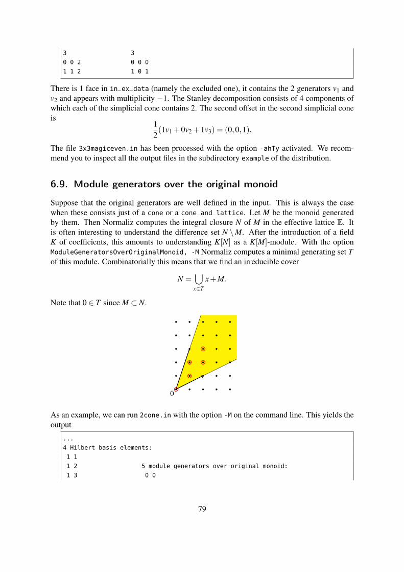
3 3

0 0 2 0 0 0

1 1 2 1 0 1

There is 1 face in in_ex_data (namely the excluded one), it contains the 2 generators v1 andv2 and appears with multiplicity −1. The Stanley decomposition consists of 4 components ofwhich each of the simplicial cone contains 2. The second offset in the second simplicial coneis

12(1v1 +0v2 +1v3) = (0,0,1).

The file 3x3magiceven.in has been processed with the option -ahTy activated. We recom-mend you to inspect all the output files in the subdirectory example of the distribution.

6.9. Module generators over the original monoid

Suppose that the original generators are well defined in the input. This is always the casewhen these consists just of a cone or a cone_and_lattice. Let M be the monoid generatedby them. Then Normaliz computes the integral closure N of M in the effective lattice E. Itis often interesting to understand the difference set N \M. After the introduction of a fieldK of coefficients, this amounts to understanding K[N] as a K[M]-module. With the optionModuleGeneratorsOverOriginalMonoid, -M Normaliz computes a minimal generating set Tof this module. Combinatorially this means that we find an irreducible cover

N =⋃x∈T

x+M.

Note that 0 ∈ T since M ⊂ N.

0

As an example, we can run 2cone.in with the option -M on the command line. This yields theoutput

...

4 Hilbert basis elements:

1 1

1 2 5 module generators over original monoid:

1 3 0 0

79

2 1 1 1

1 2

2 extreme rays: 2 2

1 3 2 3

2 1

In the nonpointed case Normaliz can only compute the module generators of N/N0 overM/(M ∩N0) where N0 is the unit group of N. If M0 6= M0, this is not a system of genera-tors of M over N.

6.9.1. An inhomogeneous example

Let us have a look at a very simple input file (genmod_inhom2.in):

amb_space 2

cone 2

0 3

2 0

vertices 1

0 0 1

ModuleGeneratorsOverOriginalMonoid

The cone is the positive orthant that we have turned into a polyhedron by adding the vertex(0,0). The original monoid is generated by (2,0) and (0,3).

In addition to the original monoid M and its integral closure N we have a third object, namelythe module P of lattice points in the polyhedron.We compute

1. the system of generators of P over N (the module generators) and

2. the system of generators of P over N (the module generators over original monoid).

We do not compute the system of generators of N over M (that we get in the homogeneouscase).

The output:

1 module generators




6 module generators over original monoid

3 support hyperplanes of polyhedron (homogenized)




internal index = 6


80


dehomogenization:

0 0 1

module rank = 1

***********************************************************************


0 0 1


0 1 0

1 0 0


0 0 1


0 1 0

1 0 0

6 module generators over original monoid:

0 0 1

0 1 1

0 2 1

1 0 1

1 1 1

1 2 1

3 support hyperplanes of polyhedron (homogenized):

0 0 1

0 1 0

1 0 0

6.10. Precomputed support hyperplanes

Computing the support hyperplanes can be a very time consuming task, and if it has beenthe first step in the exploration of a difficult example, it may be desirable, to use the supporthyperplanes as additional input in order to save computation time. This is especially true ifNormaliz must do an intermediate computation of the support hyperplanes because of a largenumber of simplicial cones to be evaluated. The file 2cone_supp.in is just a toy example:

81

amb_space 2

cone 2

2 1

1 3

support_hyperplanes 2

-1 2

3 -1

As pointed out in Section 3.3.1, Normaliz must trust you—here is no way of checking thecorrectness of this input without recomputing it.

6.11. Shift, denominator, quasipolynomial and multiplicity

In this section we discuss the interplay of shift, denominator of the grading and the quasipoly-nomial. As long as the denominator is 1, the situation is very simple and no ambiguity arises.See Section 2.9. We modify the example from that section as follows (InhomIneq_7.in):

amb_space 2

inhom_inequalities 3

0 2 1

0 -2 3

2 -2 3

grading

7 0

The output related to the grading is

grading:

7 0 0


module rank = 2

multiplicity = 2

Hilbert series:

1 1


1: 1

shift = -1


Hilbert polynomial:

2

82


The Hilbert series computed by hand is

t−7 +11− t7 .

We obtain it from the output as follows. The printed series is

1+ t1− t

.

Now the shift is applied and yieldst−1 +1

1− t.

Finally we make the substitution t 7→ t7, and obtain the desired result.

Now we add the complication x1 + x2 ≡−1 mod 8 ((InhomIneq_7_8.in):

amb_space 2

inhom_inequalities 3

0 2 1

0 -2 3

2 -2 3

grading

7 0

inhom_congruences 1

1 1 1 8

The result:grading:

7 0 0


module rank = 2

multiplicity = 1/4

Hilbert series:

1 0 0 0 0 0 0 1


8: 1

shift = -1



83

-1 1 -1 1 -1 1 -1


1: 1 4: 1 8: 1


0: 0 4: 0

1: 0 5: 0

2: 0 6: 1

3: 0 7: 1


The printed Hilbert series is1+ t7

1− t8 .

The application of the shift yieldst−1 + t6

1− t8 .

the correct result for the divided grading. The Hilbert quasipolynomial is computed for thedivided grading, as already explained in Section 2.6.1. As a last step, we can apply the substi-tution t 7→ t7 in order obtain the Hilbert series

t−7 + t42

1− t56

for the original grading.

Like the quasipolynomial, the multiplicity is computed for the divided grading.

6.12. A very large computation

The example CondEffPlur.in is one of the largest that Normaliz has mastered. The goal is tocompute the Condorcet efficiency of plurality voting for 4 candidates (see [10] and the refer-ences therein), even in the refined form of the Hilbert series. The Hilbert basis computationis extremely fast in DualMode so that it can be used as input. We tried three different setups(each with 30 parallel threads):

input triangulation size determinant sum computation timeinequalities 347,225,775,338 4,111,428,313,448 112:43:17 h

inequalities, -b 288,509,390,884 1,509,605,641,358 84:26:19 hHilbert basis, -b 335,331,680,623 1,433,431,230,802 97:50:05 h

The results show that the determinant sum of the bottom decomposition based on the extremerays (resulting from dualizing the input cone) comes very close to the absolute minimum thatis reached by the Hilbert basis as input. The latter leads to a finer triangulation, which, despiteof the smaller determinant sum, increases the computation time.

84

As long as the determinants are rather small (as in this computation), the two cases det = 1and det > 1 make the difference in computation complexity. In the first case Normaliz mustsolve 1 or 2 linear systems for the simplicial cone, in the latter 2 or 3.

Note: though Normaliz can compute this example, it is really a case for NmzIntegrate; see [8].It converts the computation time from days to hours.

7. Optional output files

When one of the options Files,-f or AllFiles, -a is activated, Normaliz writes additionaloutput files whose names are of type <project>.<type>. (Note that the options -T, Triangulation

and -y, StanleyDec as well as the options calling NmzIntegrate also write files in addition to<project>.out.) Moreover one can select the optional output files individually via commandline options. Most of these files contain matrices in a simple format:

<m>

<n>

<x_1>

...

<x_m>

where each row has <n> entries. Exceptions are the files with suffixes cst, inv, esp.

As pointed out in Section 5.4, the optional output files for the integer hull are the same as forthe original computation, as far as their content has been computed.

7.1. The homogeneous case

The option -f makes Normaliz write the following files:

gen contains the Hilbert basis. If you want to use this file as an input file and reproduce thecomputation results, then you must make it a matrix of type cone_and_lattice (andadd the dehomogenization in the inhomogeneous case).

cst contains the constraints defining the cone and the lattice in the same format as theywould appear in the input: matrices of types constraints following each other. Eachmatrix is concluded by the type of the constraints. Empty matrices are indicated by 0 asthe number of rows. Therefore there will always be at least 3 matrices.If a grading is defined, it will be appended. Therefore this file (with suffix in) as inputfor Normaliz will reproduce the Hilbert basis and all the other data computed, at leastin principle.

inv contains all the information from the file out that is not contained in any of the otherfiles.

If -a is activated, then the following files are written additionally:

ext contains the extreme rays of the cone.

85

ht1 contains the degree 1 elements of the Hilbert basis if a grading is defined.egn,esp These contain the Hilbert basis and support hyperplanes in the coordinates with re-

spect to a basis of E. esp contains the grading and the dehomogenization in the coordi-nates of E. Note that no equations for C∩E or congruences for E are necessary.

lat contains the basis of the lattice E.mod contains the module generators of the integral closure modulo the original monoid.msp contains the basis of the maximal subspace.

In order to select one or more of these files individually, add an option of type --<suffix> tothe command line where <suffix> can take the values

gen, cst, inv, ext, ht1, egn, esp, lat, mod, typ, msp

The type typ is not contained in Files or AllFiles since it can be extremely large. It is thematrix format described above. It is the product of the matrices corresponding to egn and thetranspose of esp. In other words, the linear forms representing the support hyperplanes of thecone C are evaluated on the Hilbert basis. The resulting matrix, with the generators corre-sponding to the rows and the support hyperplanes corresponding to the columns, is written tothis file.

The suffix typ is motivated by the fact that the matrix in this file depends only on the isomor-phism type of monoid generated by the Hilbert basis (up to row and column permutations). Inthe language of [4] it contains the standard embedding.

Note: the explicit choice of an optional output file does not imply a computation goal. Out-put files that would contain unknown data are simply not written without a warning or errormessage.

7.2. Modifications in the inhomogeneous case

The optional output files are a subset of those that can be produced in the homogeneous case.The main difference is that the generators of the solution module and the Hilbert basis of therecession monoid appear together in the file gen. They can be distinguished by evaluating thedehomogenization on them (simply the last component with inhomogeneous input), and thesame applies to the vertices of the polyhedron and extreme rays of the recession cone. The filecst contains the constraints defining the polyhedron and the recession module in conjunctionwith the dehomogenization, which is also contained in the cst file, following the constraints.

With -a the files egn and esp are produced. These files contain gen and the support hyper-planes of the homogenized cone in the coordinates of E, as well as the dehomogenization.

8. Performance

86

8.1. Parallelization

The executables of Normaliz have been compiled for parallelization on shared memory sys-tems with OpenMP. Parallelization reduces the “real” time of the computations considerably,even on relatively small systems. However, one should not underestimate the administrationaloverhead involved.

• It is not a good idea to use parallelization for very small problems.• On multi-user systems with many processors it may be wise to limit the number of

threads for Normaliz somewhat below the maximum number of cores.

The number of parallel threads can be limited by the Normaliz option -x (see Section 5.3) orby the commands

export OMP_NUM_THREADS=<T> (Linux/Mac)

or

set OMP_NUM_THREADS=<T> (Windows)

where <T> stands for the maximum number of threads accessible to Normaliz. For example,we often use

export OMP_NUM_THREADS=20

on a multi-user system system with 24 cores.

Limiting the number of threads to 1 forces a strictly serial execution of Normaliz.

The paper [8] contains extensive data on the effect of parallelization. On the whole Normalizscales very well. However, the dual algorithm often performs best with mild parallelization,say with 4 or 6 threads.

8.2. Running large computations

Normaliz can cope with very large examples, but it is usually difficult to decide a prioriwhether an example is very large, but nevertheless doable, or simply impossible. Thereforesome exploration makes sense.

See [8] for some very large computations. The following hints reflect the authors’ experiencewith them.

(1) Run Normaliz with the option -cs and pay attention to the terminal output. The numberof extreme rays, but also the numbers of support hyperplanes of the intermediate cones areuseful data.

(2) In many cases the most critical size parameter is the number of simplicial cones in thetriangulation. It makes sense to determine it as the next step. Even with the fastest potential

87

evaluation (option -v), finding the triangulation takes less time, say by a factor between 3 and10. Thus it makes sense to run the example with -t in order to explore the size.

As you can see from [8], Normaliz has successfully evaluated triangulations of size ≈ 5 ·1011

in dimension 24.

(3) Another critical parameter are the determinants of the generator matrices of the simplicialcones. To get some feeling for their sizes, one can restrict the input to a subset (of the extremerays computed in (1)) and use the option -v or the computation goal TriangulationDetSum ifthere is no grading.

The output file contains the number of simplicial cones as well as the sum of the absolutevalues of the determinants. The latter is the number of vectors to be processed by Normaliz intriangulation based calculations.

The number includes the zero vector for every simplicial cone in the triangulation. The zerovector does not enter the Hilbert basis calculation, but cannot be neglected for the Hilbertseries.

Normaliz has mastered calculations with > 1015 vectors.

(4) If the triangulation is small, we can add the option -T in order to actually see the triangu-lation in a file. Then the individual determinants become visible.

(5) If a cone is defined by inequalities and/or equations consider the dual mode for Hilbertbasis calculation, even if you also want the Hilbert series.

(6) The size of the triangulation and the size of the determinants are not dangerous for memoryby themselves (unless -T or -y are set). Critical magnitudes can be the number of supporthyperplanes, Hilbert basis candidates, or degree 1 elements.

9. Distribution and installation

In order to install Normaliz you should first download the basic package containing the docu-mentation, examples, source code, jNormaliz, NmzIntegrate and the packages for Singular andMacaulay2. Then unzip the downloaded file Normaliz3.0.zip in a directory of your choice.(Any other downloaded zip file for Normaliz should be unzipped in this directory, too.)

This process will create a directory Normaliz3.0 (called Normaliz directory) and several sub-directories in Normaliz3.0. The names of the subdirectories created are self-explanatory.Nevertheless we give an overview:

• In the main directory Normaliz3.0 you should find jNormaliz.jar, Copying and sub-directories.• The subdirectory source contains the source files. The subdirectory genEhrhart con-

tains the NmzIntegrate source.• The subdirectory doc contains the file you are reading and further documentation.• In the subdirectory example are the input and output files for some examples. It contains

all input files of examples of this documentation, except the toy examples of Section 3.

88

• Automated tests which run Normaliz on different inputs and options are contained inthe subdirectory test.• The subdirectory singular contains the SINGULAR library normaliz.lib and a PDF

file with documentation.• The subdirectory macaulay2 contains the MACAULAY2 package Normaliz.m2.• The subdirectory lib contains libraries for jNormaliz.

We provide executables for Windows, Linux (each in a 32 bit and a 64 bit version) and Mac.Download the archive file corresponding to your system Normaliz3.0<systemname>.zip andunzip it. This process will store the executables of Normaliz and NmzIntegrate in the directoryNormaliz3.0. In case you want to run Normaliz from the command line or use it from othersystems, you may have to copy the executables to a directory in the search path for executables.

Please remove old versions of normaliz, norm64 and normbig from your search path.

10. Compilation

We only describe the compilation of Normaliz. See the documentation of NmzIntegrate for itscompilation.

10.1. General

For compiling Normaliz the following libraries are needed:

• GMP including the C++ wrapper (libgmpxx and libgmp)• boost (headers only)• OpenMP 3.0 enabled compiler (to use parallelization, optional)

Furthermore we require some C++11 features (e.g. std::exception_ptr), supported by:

• GNU g++ 4.4,• clang++ 2.9,• Intel icpc 12.0

See https://github.com/Normaliz/Normaliz/issues/26 for a more detailed discussion.

The mentioned compilers are also able to handle OpenMP 3.0, with the exception of clang++,there the first OpenMP support was introduced in 3.7.

In the following we describe the configuration/build process using cmake. This has capabil-ities to find libraries and allows to change settings in a nice interface. It supports the com-pilation of the library as a static and a dynamic version and the installation of the library.Furthermore it can also be used to compile Normaliz including SCIP or offloads to Intel XeonPhi cards.

We will only handle the basic use of cmake for compilation, see the file source/INSTALL foradditional information, especially on how to use customized paths.

89

https://github.com/Normaliz/Normaliz/issues/26

10.2. Linux

On Ubuntu the following packages should be installed:

sudo apt-get install g++ libgmp-dev libboost-dev cmake cmake-curses-gui

We assume you start in the normaliz root dir (with subdirs source, example, ...).

1. Create a build directory where normaliz will be build and cd into it, e.g.

mkdir BUILD; cd BUILD

2. Initial configuration, have a look at the next sections for further information about theconfiguration.

cmake ../source

3. [Optional] Check configuration and maybe edit something (note the two ’c’s at thebeginning)

ccmake ../source

In the ccmake interface you can use this work flow:

• c (configure)• change entries if you like (use cursor keys and enter), then press c again• g (generate and exit)

4. compile

make

5. install it

make install

This will install the library headers, the produced libnormaliz and the normaliz exe-cutable. The installation path can be changed with ccmake (CMAKE_INSTALL_PREFIX).

10.3. Mac OS X

Currently Apple does not supply a compiler which supports OpenMP. We recommend the useof a current gcc.

To install this, and other prerequisites, we recommend using a package manager such asFink http://www.finkproject.org/, Homebrew http://brew.sh/, or MacPort https://www.macports.org/.

You can then follow the instructions for Linux.

10.4. Windows

One can compile Windows executables with the Cygwin port of GCC. Unfortunately it is notcompatible to OpenMP.

90

http://www.finkproject.org/

http://brew.sh/

https://www.macports.org/

https://www.macports.org/

Using Visual Studio is a bit tricky. Microsoft’s C++ compiler does not support OpenMP 3.0.Creating a Normaliz Visual Studio project via cmake is currently not fully supported. Thesupplied executables are compiled with icpc with a manually created project. Please contactus if you want to build Normaliz on Windows.

11. Copyright and how to cite

Normaliz 3.0 is free software licensed under the GNU General Public License, version 3. Youcan redistribute it and/or modify it under the terms of the GNU General Public License aspublished by the Free Software Foundation, either version 3 of the License, or (at your option)any later version.

It is distributed in the hope that it will be useful, but WITHOUT ANY WARRANTY; withouteven the implied warranty of MERCHANTABILITY or FITNESS FOR A PARTICULARPURPOSE. See the GNU General Public License for more details.

You should have received a copy of the GNU General Public License along with the program.If not, see http://www.gnu.org/licenses/.

Please refer to Normaliz in any publication for which it has been used:

W. Bruns, B. Ichim, T. Römer, R. Sieg and C. Söger: Normaliz. Algorithms for rationalcones and affine monoids. Available at http://normaliz.uos.de

The corresponding \bibitem:

\bibitem{Normaliz} W. Bruns, B. Ichim, T. R\"omer, R. Sieg and C. S\"oger:

Normaliz. Algorithms for rational cones and affine monoids.

Available at \url{http://normaliz.uos.de}.

A BibTeX entry:

@Misc{Normaliz,

author = {W. Bruns and B. Ichim and T. R\"omer and R. Sieg and C. S\"oger},

title = Normaliz. Algorithms for rational cones and affine monoids,

howpublished ={Available at \url{http://normaliz.uos.de}}

It is now customary to evaluate mathematicians by such data as numbers of publications,citations and impact factors. The data bases on which such dubious evaluations are based donot list mathematical software. Therefore we ask you to cite the article [8] in addition. This isvery helpful for the younger members of the team.

91

http://www.gnu.org/licenses/


A. Mathematical background and terminology

For a coherent and thorough treatment of the mathematical background we refer the reader to[4].

A.1. Polyhedra, polytopes and cones

An affine halfspace of Rd is a subset given as

H+λ= {x : λ (x)≥ 0},

where λ is an affine form, i.e., a non-constant map λ : Rd→R, λ (x) = α1x1+ · · ·+αdxd +β

with α1, . . . ,αd,β ∈ R. If β = 0 and λ is therefore linear, then the halfspace is called linear.The halfspace is rational if λ is rational, i.e., has rational coordinates. If λ is rational, wecan assume that it is even integral, i.e., has integral coordinates, and, moreover, that these arecoprime. Then λ is uniquely determined by H+

λ. Such integral forms are called primitive, and

the same terminology applies to vectors.

Definition 1. A (rational) polyhedron P is the intersection of finitely many (rational) halfs-paces. If it is bounded, then it is called a polytope. If all the halfspaces are linear, then P is acone.

The dimension of P is the dimension of the smallest affine subspace aff(P) containing P.

A support hyperplane of P is an affine hyperplane H that intersects P, but only in such a waythat H is contained in one of the two halfspaces determined by H. The intersection H ∩P iscalled a face of P. It is a polyhedron (polytope, cone) itself. Faces of dimension 0 are calledvertices, those of dimension 1 are called edges (in the case of cones extreme rays), and thoseof dimension dim(P)−1 are facets.

When we speak of the support hyperplanes of P, then we mean those intersecting P in a facet.Their halfspaces containing P cut out P from aff(P). If dim(P) = d, then they are uniquelydetermined (up to a positive scalar).

The constraints by which Normaliz describes polyhedra are

(1) linear equations for aff(P) and(2) linear inequalities (simply called support hyperplanes) cutting out P from aff(P).

In other words, the constraints are given by a linear system of equations and inequalities,and a polyhedron is nothing else than the solution set of a linear system of inequalities andequations. It can always be represented in the form

Ax≥ b, A ∈ Rm×d,b ∈ Rm,

if we replace an equation by two inequalities.

92

A.2. Cones

The definition describes a cone by constraints. One can equivalently describe it by generators:

Theorem 2 (Minkowski-Weyl). The following are equivalent for C ⊂ Rd;

1. C is a (rational) cone;

2. there exist finitely many (rational) vectors x1, . . . ,xn such that

C = {a1x1 + · · ·+anxn : a1, . . . ,an ∈ R+}.

By R+ we denote the set of nonnegative real numbers; Q+ and Z+ are defined in the sameway.

The conversion between the description by constraints and that by generators is one of thebasic tasks of Normaliz. It uses the Fourier-Motzkin elimination.

Let C0 be the set of those x ∈ C for which −x ∈ C as well. It is the largest vector subspacecontained in C. A cone is pointed if C0 = 0. If a rational cone is pointed, then it has uniquelydetermined extreme integral generators. These are the primitive integral vectors spanning theextreme rays. These can also be defined with respect to a sublattice L of Zd , provided C iscontained in RL. If a cone is not pointed, then Normaliz computes the extreme rays of thepointed C/C0 and lifts them to C. (Therefore they are only unique modulo C0.)

The dual cone C∗ is given by

C∗ = {λ ∈ (Rd)∗ : λ (x)≥ 0 for all x ∈C}.

Under the identification Rd = (Rd)∗∗ one has C∗∗ =C. Then one has

dimC0 +dimC∗ = d.

In particular, C is pointed if and only if C∗ is full dimensional, and this is the criterion forpointedness used by Normaliz. Linear forms λ1, . . . ,λn generate C∗ if and only if C is theintersection of the halfspaces H+

λi. Therefore the conversion from constraints to generators

and its converse are the same task, except for the exchange of Rd and its dual space.

A.3. Polyhedra

In order to transfer the Minkowski-Weyl theorem to polyhedra it is useful to homogenizecoordinates by embedding Rd as a hyperplane in Rd+1, namely via

κ : Rd → Rd+1, κ(x) = (x,1).

If P is a (rational) polyhedron, then the closure of the union of the rays from 0 through thepoints of κ(P) is a (rational) cone C(P), called the cone over P. The intersection C(P)∩(Rd×{0}) can be identified with the recession (or tail) cone

rec(P) = {x ∈ Rd : y+ x ∈ P for all y ∈ P}.

93

It is the cone of unbounded directions in P. The recession cone is pointed if and only if P hasat least one bounded face, and this is the case if and only if it has a vertex.

The theorem of Minkowski-Weyl can then be generalized as follows:

Theorem 3 (Motzkin). The following are equivalent for a subset P 6= /0 of Rd:

1. P is a (rational) polyhedron;

2. P = Q+C where Q is a (rational) polytope and C is a (rational) cone.

If P has a vertex, then the smallest choice for Q is the convex hull of its vertices, and C = rec(P)is uniquely determined.

The convex hull of a subset X ∈ Rd is

conv(X) = {a1x1 + · · ·+anxn : n≥ 1,x1, . . . ,xn ∈ X ,a1, . . . ,an ∈ R+,a1 + · · ·+an = 1}.

Clearly, P is a polytope if and only if rec(P) = {0}, and the specialization to this case oneobtains Minkowski’s theorem: a subset P of Rd is a polytope if and only if it is the convexhull of a finite set. A lattice polytope is distinguished by having integral points as vertices.

Normaliz computes the recession cone and the polytope Q if P is defined by constraints.Conversely it finds the constraints if the vertices of Q and the generators of C are specified.

Suppose that P is given by a system

Ax≥ b, A ∈ Rm×d, b ∈ Rm,

of linear inequalities (equations are replaced by two inequalities). Then C(P) is defined by thehomogenized system

Ax− xd+1b≥ 0

whereas the rec(P) is given by the associated homogeneous system

Ax≥ 0.

It is of course possible that P is empty if it is given by constraints since inhomogeneoussystems of linear equations and inequalities may be unsolvable. By abuse of language we callthe solution set of the associated homogeneous system the recession cone of the system.

Via the concept of dehomogenization, Normaliz allows for a more general approach. Thedehomogenization is a linear form δ on Rd+1. For a cone C in Rd+1 and a dehomogenizationδ , Normaliz computes the polyhedron P = {x∈ C : δ (x) = 1} and the recession cone C = {x∈C : δ (x) = 0}. In particular, this allows other choices of the homogenizing coordinate. (Oftenone chooses x0, the first coordinate then.)

In the language of projective geometry, δ (x) = 0 defines the hyperplane at infinity.

94

A.4. Affine monoids

An affine monoid M is a finitely generated submonoid of Zd for some d ≥ 0. This means:0 ∈M, M+M ⊂M, and there exist x1, . . . ,xn such that

M = {a1x1 + · · ·+anxn : a1, . . . ,an ∈ Z+}.

We say that x1, . . . ,xn is a system of generators of M. A monoid M is positive if x ∈ M and−x ∈M implies x = 0. An element x in a positive monoid M is called irreducible if it has nodecomposition x = y+ z with y,z ∈ M, y,z 6= 0. The rank of M is the rank of the subgroupgp(M) of Zd generated by M. (Subgroups of Zd are also called sublattices.) For certain aspectsof monoid theory it is very useful (or even necessary) to introduce coefficients from a field K(or a more general commutative ring) and consider the monoid algebra K[M].

Theorem 4 (van der Corput). Every positive affine monoid M has a unique minimal system ofgenerators, given by its irreducible elements.

We call the minimal system of generators the Hilbert basis of M. Normaliz computes Hilbertbases of a special type of affine monoid:

Theorem 5 (Gordan’s lemma). Let C ⊂ Rd be a (pointed) rational cone and let L ⊂ Zd be asublattice. Then C∩L is a (positive) affine monoid.

The monoids M =C∩L of the theorem have the pleasant property that the group of units M0(i.e., elements whose inverse also belongs to M) splits off as a direct summand. ThereforeM/M0 is a well-defied affine monoid. If M is not positive, then Normaliz computes a Hilbertbasis of M/M0 and lifts it to M.

Let M ⊂ Zd be an affine monoid, and let N ⊃M be an overmonoid (not necessarily affine), forexample a sublattice L of Zd containing M.

Definition 6. The integral closure (or saturation) of M in N is the set

MN = {x ∈ N : kx ∈M for some k ∈ Z,k > 0}.

If MN = M, one calls M integrally closed in N.

The integral closure M of M in gp(M) is its normalization. M is normal if M = M.

The integral closure has a geometric description:

Theorem 7.MN = cone(M)∩N.

Combining the theorems, we can say that Normaliz computes integral closures of affinemonoids in lattices, and the integral closures are themselves affine monoids as well. (Moregenerally, MN is affine if M and N are affine.)

95

In order to specify the intersection C∩ L by constraints we need a system of homogeneousinequalities for C. Every sublattice of Zd can be written as the solution set of a combined sys-tem of homogeneous linear diophantine equations and a homogeneous system of congruences(this follows from the elementary divisor theorem). Thus C∩ L is the solution set of a ho-mogeneous linear diophantine system of inequalities, equations and congruences. Conversely,the solution set of every such system is a monoid of type C∩L.

In the situation of Theorem 7, if gp(N) has finite rank as a gp(M)-module, MN is even a finitelygenerated module over M. I.e., there exist finitely many elements y1, . . . ,ym ∈ MN such thatMN =

⋃mi=1 M + yi. Normaliz computes a minimal system y1, . . . ,ym and lists the nonzero

yi as a system of module generators of MN modulo M. We must introduce coefficients tomake this precise: Normaliz computes a minimal system of generators of the K[M]-moduleK[MN ]/K[M].

A.5. Affine monoids from binomial ideals

Let U be a subgroup of Zn. Then the natural image M of Zn+ ⊂ Zn in the abelian group

G = Zn/U is a submonoid of G. In general, G is not torsionfree, and therefore M may notbe an affine monoid. However, the image N of M in the lattice L = G/torsion(G) is an affinemonoid. Given U , Normaliz chooses an embedding L ↪→ Zr, r = n− rankU , such that Nbecomes a submonoid of Zr

+. In general there is no canonical choice for such an embedding,but one can always find one, provided N has no invertible element except 0.

The typical starting point is an ideal J ⊂ K[X1, . . . ,Xn] generated by binomials

Xa11 · · ·X

ann −Xb1

1 · · ·Xbnn .

The image of K[X1, . . . ,Xn] in the residue class ring of the Laurent polynomial ring S =K[X±1

1 , . . . ,X±1n ] modulo the ideal JS is exactly the monoid algebra K[M] of the monoid M

above if we let U be the subgroup of Zn generated by the differences

(a1, . . . ,an)− (b1, . . . ,bn).

Ideals of type JS are called lattice ideals if they are prime. Since Normaliz automaticallypasses to G/torsion(G), it replaces JS by the smallest lattice ideal containing it.

A.6. Lattice points in polyhedra

Let P ⊂ Rd be a rational polyhedron and L ⊂ Zd be an affine sublattice, i.e., a subset w+L0where w ∈ Zd and L0 ⊂ Zd is a sublattice. In order to investigate (and compute) P∩L oneagain uses homogenization: P is extended to C(P) and L is extended to L = L0 +Z(w,1).Then one computes C(P)∩L . Via this “bridge” one obtains the following inhomogeneousversion of Gordan’s lemma:

96

Theorem 8. Let P be a rational polyhedron with vertices and L = w+L0 an affine lattice asabove. Set recL(P) = rec(P)∩L0. Then there exist x1, . . . ,xm ∈ P∩L such that

P∩L = {(x1 + recL(P))∩·· ·∩ (xm + recL(P))}.

If the union is irredundant, then x1, . . . ,xm are uniquely determined.

The Hilbert basis of recL(P) is given by {x : (x,0)∈Hilb(C(P)∩L )} and the minimal systemof generators can also be read off the Hilbert basis of C(P)∩L : it is given by those x for which(x,1) belongs to Hilb(C(P)∩L ). (Normaliz computes the Hilbert basis of C(P)∩L only at“levels” 0 and 1.)

We call recL(P) the recession monoid of P with respect to L (or L0). It is justified to call P∩La module over recL(P). In the light of the theorem, it is a finitely generated module, and it hasa unique minimal system of generators.

After the introduction of coefficients from a field K, recL(P) is turned into an affine monoidalgebra, and N = P∩L into a finitely generated torsionfree module over it. As such it has awell-defined module rank mrank(N), which is computed by Normaliz via the following com-binatorial description: Let x1, . . . ,xm be a system of generators of N as above; then mrank(N)is the cardinality of the set of residue classes of x1, . . . ,xm modulo recL(P).

Clearly, to model P∩ L we need linear diophantine systems of inequalities, equations andcongruences which now will be inhomogeneous in general. Conversely, the set of solutions ofsuch a system is of type P∩L.

A.7. Hilbert series

Normaliz can compute the Hilbert series and the Hilbert (quasi)polynomial of a graded monoid.A grading of a monoid M is simply a homomorphism deg : M→ Zg where Zg contains thedegrees. The Hilbert series of M with respect to the grading is the formal Laurent series

H(t) = ∑u∈Zg

#{x ∈M : degx = u}tu11 · · · t

ugg = ∑

x∈Mtdegx,

provided all sets {x ∈ M : degx = u} are finite. At the moment, Normaliz can only handlethe case g = 1, and therefore we restrict ourselves to this case. We assume in the followingthat degx > 0 for all nonzero x ∈ M and that there exists an x ∈ gp(M) such that degx = 1.(Normaliz always rescales the grading accordingly.) In the case of a nonpositive monoid, theseconditions must hold for M/M0, and its Hilbert series is considered as the Hilbert series of M.

The basic fact about H(t) in the Z-graded case is that it is the Laurent expansion of a rationalfunction at the origin:

Theorem 9 (Hilbert, Serre; Ehrhart). Suppose that M is a normal positive affine monoid. Then

H(t) =R(t)

(1− te)r , R(t) ∈ Z[t],

where r is the rank of M and e is the least common multiple of the degrees of the extremeintegral generators of cone(M). As a rational function, H(t) has negative degree.

97

The statement about the rationality of H(t) holds under much more general hypotheses.

Usually one can find denominators for H(t) of much lower degree than that in the theorem,and Normaliz tries to give a more economical presentation of H(t) as a quotient of two poly-nomials. One should note that it is not clear what the most natural presentation of H(t) is ingeneral (when e > 1). We discuss this problem in [8, Section 4]. The examples 2.5 and 2.6.1,may serve as an illustration.

A rational cone C and a grading together define the rational polytope Q =C∩A1 where A1 ={x : degx = 1}. In this sense the Hilbert series is nothing but the Ehrhart series of Q. Thefollowing description of the Hilbert function H(M,k) = #{x ∈M : degx = k} is equivalent tothe previous theorem:

Theorem 10. There exists a quasipolynomial q with rational coefficients, degree rankM− 1and period π dividing e such that H(M,k) = q(k) for all q≥ 0.

The statement about the quasipolynomial means that there exist polynomials q( j), j = 0, . . . ,π−1, of degree rankM−1 such that

q(k) = q( j)(k), j ≡ k (π),

andq( j)(k) = q( j)

0 +q( j)1 k+ · · ·+q( j)

r−1kr−1, r = rankM,

with coefficients q( j)i ∈Q. It is not hard to show that in the case of affine monoids all compo-

nents have the same degree r−1 and the same leading coefficient:

qr−1 =vol(Q)

(r−1)!,

where vol is the lattice normalized volume of Q (a lattice simplex of smallest possible volumehas volume 1). The multiplicity of M, denoted by e(M) is (r−1)!qr−1 = vol(Q).

Suppose now that P is a rational polyhedron in Rd , L⊂Zd is an affine lattice, and we considerN = P∩L as a module over M = recL(P). Then we must give up the condition that deg takesthe value 1 on gp(M) (see Section 6.11 for an example). But the Hilbert series

HN(t) = ∑x∈N

tdegx

is well-defined, and the qualitative statement above about rationality remain valid. However,in general the quasipolynomial gives the correct value of the Hilbert function only for k > rwhere r is the degree of the Hilbert series as a rational function.

Let m be the gcd of the numbers degx, x ∈M. (For M = {0} we set m = 1.) Then we mustdefine e(M) = e′(M)/m where e′(M) is the multiplicity of M with respect to the normalizedgrading deg/m. The multiplicity of N is given by

e(N) = mrank(N)e(M).

Since N may have generators in negative degrees, Normaliz shifts the degrees into Z+ bysubtracting a constant, called the shift. (The shift may also be positive.)

98

A.8. The class group

A normal affine monoid M has a well-defined divisor class group. It is naturally isomorphicto the divisor class group of K[M] where K is a field (or any unique factorization domain);see [4, 4.F], and especially [4, 4.56]. The class group classifies the divisorial ideals up toisomorphism. It can be computed from the standard embedding that sends an element x ofgp(M) to the vector σ(x) where σ is the collection of support forms σ1, . . . ,σs of M: Cl(M) =Zs/σ(gp(M)). Finding this quotient amounts to an application of the Smith normal form tothe matrix of σ .

B. Annotated console output

B.1. Primal mode

With./normaliz -c example/A443

we get the following terminal output.

\.....|

Normaliz 3.0 \....|

\...|

(C) The Normaliz Team, University of Osnabrueck \..|

September 2015 \.|

\|

************************************************************Compute: DefaultMode

************************************************************starting primal algorithm with full triangulation ...

Roughness 1

Generators sorted by degree and lexicographically

Generators per degree:

1: 48

Self explanatory so far (see Section 6.2 for the definition of roughness). Now the generatorsare inserted.

Start simplex 1 2 3 4 5 6 7 8 9 10 11 12 13 14 15 16 19 22 25 26 27 28 31 34

37 38 39 40 43 46

Normaliz starts by searching linearly independent generators with indices as small as possi-ble. They span the start simplex in the triangulation. The remaining generators are insertedsuccessively. (If a generator does not increase the cone spanned by the previous ones, it is notlisted, but this does not happen for A443.)

99

gen=17, 39 hyp, 4 simpl

We have now reached a cone with 39 support hyperplanes and the triangulation has 3 simplicesso far. We omit some generators until something interesting happens:

gen=35, 667 hyp, 85 pyr, 13977 simpl

In view of the number of simplices in the triangulation and the number of support hyperplanes,Normaliz has decided to build pyramids and to store them for later triangulation.

gen=36, 723 hyp, 234 pyr, 14025 simpl

...

gen=48, 4948 hyp, 3541 pyr, 14856 simpl

**************************************************level 0 pyramids remaining: 3541

**************************************************

Now these pyramids must be triangulated. They may produce not only simplices, but alsopyramids of higher level, and indeed they do so:

**************************************************all pyramids on level 0 done!


**************************************************



**************************************************1180 pyramids remaining on level 2, evaluating 2503294 simplices

At this point the preset size of the evaluation buffer for simplices has been exceeded. Normalizstops the processing of pyramids, and empties the buffer by evaluating the simplices.

||||||||||||||||||||||||||||||||||||||||||||||||||

2503294 simplices, 0 HB candidates accumulated.



**************************************************


This is a small computation, and the computation of pyramids goes level by level without thenecessity to return to a lower level. But in larger examples the buffer for level n+ 1 may befilled before level n is finished. Then it becomes necessary to go back.

100

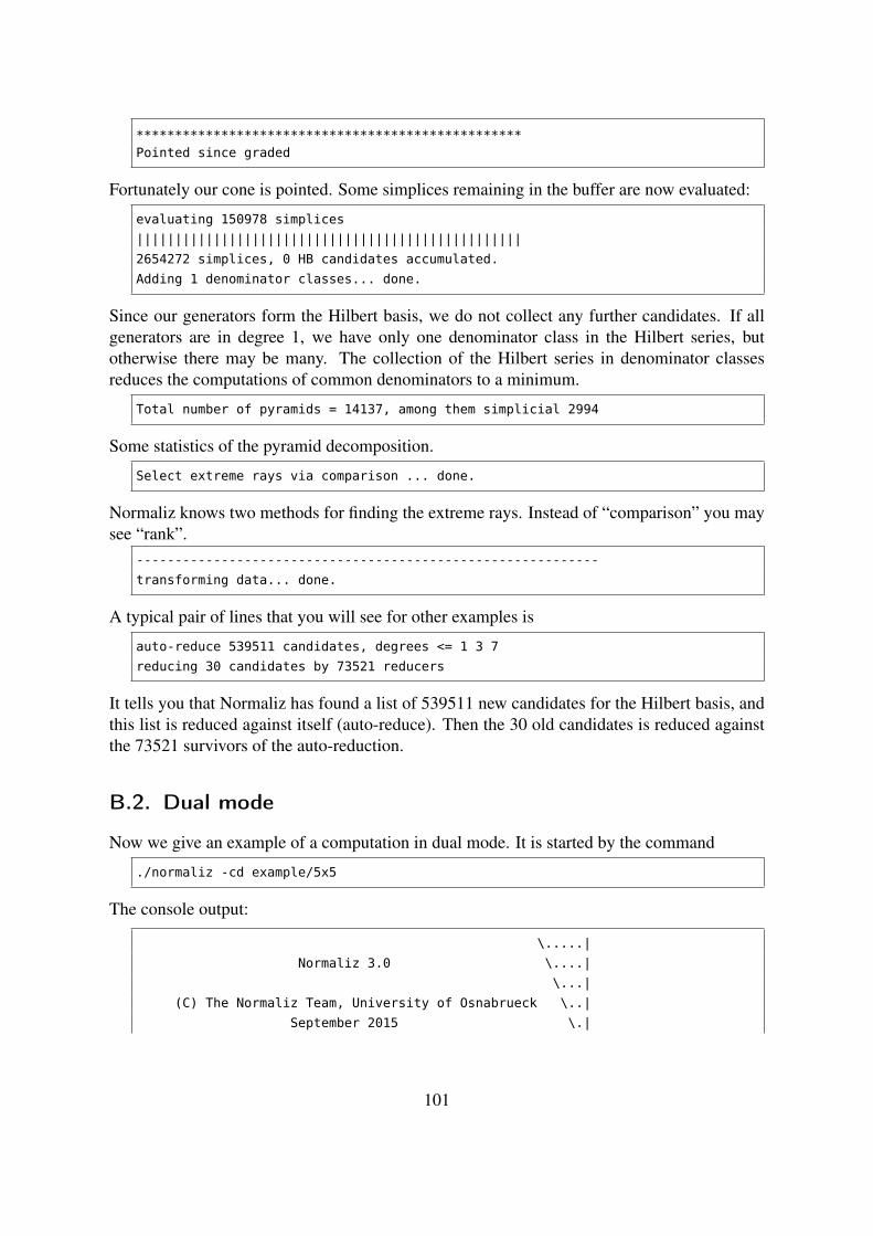
**************************************************Pointed since graded

Fortunately our cone is pointed. Some simplices remaining in the buffer are now evaluated:

evaluating 150978 simplices

||||||||||||||||||||||||||||||||||||||||||||||||||

2654272 simplices, 0 HB candidates accumulated.

Adding 1 denominator classes... done.

Since our generators form the Hilbert basis, we do not collect any further candidates. If allgenerators are in degree 1, we have only one denominator class in the Hilbert series, butotherwise there may be many. The collection of the Hilbert series in denominator classesreduces the computations of common denominators to a minimum.

Total number of pyramids = 14137, among them simplicial 2994

Some statistics of the pyramid decomposition.

Select extreme rays via comparison ... done.

Normaliz knows two methods for finding the extreme rays. Instead of “comparison” you maysee “rank”.

------------------------------------------------------------

transforming data... done.

A typical pair of lines that you will see for other examples is

auto-reduce 539511 candidates, degrees <= 1 3 7

reducing 30 candidates by 73521 reducers

It tells you that Normaliz has found a list of 539511 new candidates for the Hilbert basis, andthis list is reduced against itself (auto-reduce). Then the 30 old candidates is reduced againstthe 73521 survivors of the auto-reduction.

B.2. Dual mode

Now we give an example of a computation in dual mode. It is started by the command

./normaliz -cd example/5x5

The console output:

\.....|

Normaliz 3.0 \....|

\...|

(C) The Normaliz Team, University of Osnabrueck \..|

September 2015 \.|

101

\|

************************************************************Compute: DualMode

No inequalities specified in constraint mode, using non-negative orthant.

Indeed, we have used equations as the input.

************************************************************computing Hilbert basis ...

==================================================

cut with halfspace 1 ...

Final sizes: Pos 1 Neg 1 Neutral 0

The cone is cut out from the space of solutions of the system of equations (in this case) bysuccessive intersections with halfspaces defined by the inequalities. After such an intersectionwe have the positive half space, the “neutral” hyperplane and the negative half space. The finalsizes given are the numbers of Hilbert basis elements strictly in the positive half space, strictlyin the negative half space, and in the hyperplane. This pattern is repeated until all hyperplaneshave been used.

==================================================



We leave out some hyperplanes . . .

==================================================


auto-reduce 1159 candidates, degrees <= 13 27


==================================================


Positive: 1027 Negative: 367

..................................................


Sometimes reduction takes some time, and then Normaliz may issue a message on “auto-reduction” organized by degree (chosen for the algorithm, not defined by the given grading).The line of dots is printed is the computation of new Hilbert basis candidates takes time, andNormaliz wants to show you that it is not sleeping. Normaliz shows you the number of positiveand negative partners that must be pared produce offspring.

==================================================


Positive: 1856 Negative: 653

..................................................

auto-reduce 1899 candidates, degrees <= 19 39

102


All hyperplanes have been taken care of.

Find extreme rays

Find relevant support hyperplanes

Well, in connection with the equations, some hyperplanes become superfluous. In the outputfile Normaliz will list a minimal set of support hyperplanes that together with the equationsdefine the cone.

Hilbert basis 4828

The number of Hilbert basis elements computed is the sum of the last positive and neutralnumbers.

Find degree 1 elements

The input file contains a grading.

transforming data... done.

The computation of the new Hilbert basis after the intersection with the new hyperplane pro-ceeds in rounds, and there be many rounds . . . (not in the above example). then you can seeterminal output like

Round 100

Round 200

Round 300

Round 400

Round 500

C. Normaliz 2 input syntax

A Normaliz 2 input file contains a sequence of matrices. Comments or options are not allowedin it. A matrix has the format

<m>

<n>

<x_1>

...

<x_m>

<type>

where <m> denotes the number of rows, <n> is the number of columns and <x_1>...<x_n> arethe rows with <m> entries each. All matrix types of Normaliz 3 are allowed (with Normaliz 3),also grading and dehomogenization. These vectors must be encoded as matrices with 1 row.

103

The optional output files of with suffix cst are still in this format. Just create one and inspectit.

D. libnormaliz

The kernel of Normaliz is the C++ class library libnormaliz. It implements all the classes that arenecessary for the computations. The central class is Cone. It realizes the communication with thecalling program and starts the computations most of which are implemented in other classes. In thefollowing we describe th class Cone; other classes of libnormaliz may follow in the future.

Of course, Normaliz itself is the prime example for the use of libnormaliz, but it is rather complicatedbecause of the input and output it must handle. Therefore we have a added a simple example programat the end of this introduction.

libnormaliz defines its own name space. In the following we assume that

using namespace std;

using namespace libnormaliz;

have been declared. It is clear that opening these name spaces is dangerous. In this documentation weonly do it to avoid constant repetition of std:: and libnormaliz::

D.1. Integer type as a template parameter

A cone can be constructed for two integer types, long long and mpz_class. It is reasonable to choosempz_class since the main computations will then be tried with long long and restarted with mpz_class

if long long cannot store the results. This internal change of integer type is not possible if the coneis constructed for long long. (Nevertheless, the linear algebra routines can use mpz_class locally ifintermediate results exceed long long; have a look into matrix.cpp.)

Internally the template parameter is called Integer. In the following we assume that the integer typehas been fixed as follows:

typedef mpz_class Integer;

The internal passage from mpz_class to long long can be suppressed by

MyCone.deactivateChangeOfPrecision();

where we assume that MyCone has been constructed as described in the next section.

D.1.1. Alternative integer types

The predefined alternative to mpz_class is long long. It is possible to use libnormaliz with otherinteger types than mpz_class or long long, but we have tested only these types.

In an alternative configuration you have to include libnormaliz-all.cpp. (In this case you do notneed to link libnormaliz.a). If you want to use other types, you probably have to implement someconversion functions which you can find in integer.h. Namely the functions

104

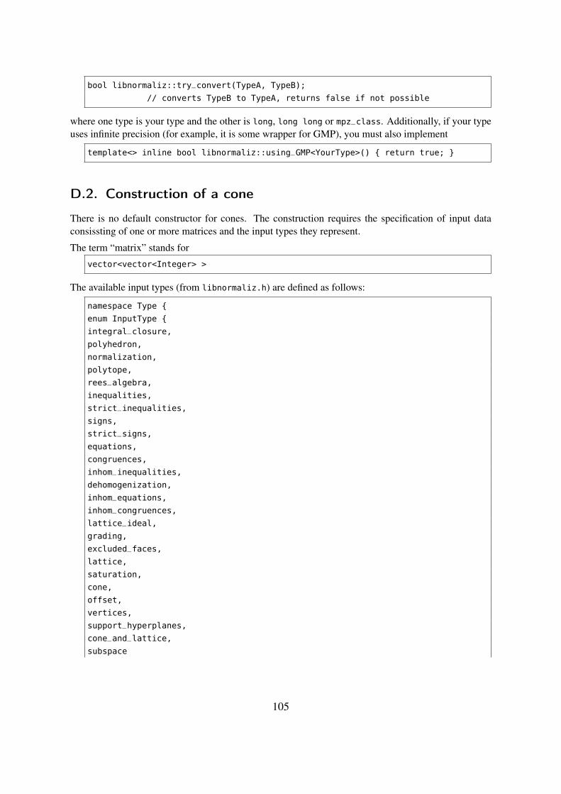
bool libnormaliz::try_convert(TypeA, TypeB);

// converts TypeB to TypeA, returns false if not possible

where one type is your type and the other is long, long long or mpz_class. Additionally, if your typeuses infinite precision (for example, it is some wrapper for GMP), you must also implement

template<> inline bool libnormaliz::using_GMP<YourType>() { return true; }

D.2. Construction of a cone

There is no default constructor for cones. The construction requires the specification of input dataconsissting of one or more matrices and the input types they represent.

The term “matrix” stands for

vector<vector<Integer> >

The available input types (from libnormaliz.h) are defined as follows:

namespace Type {

enum InputType {

integral_closure,

polyhedron,

normalization,

polytope,

rees_algebra,

inequalities,

strict_inequalities,

signs,

strict_signs,

equations,

congruences,

inhom_inequalities,

dehomogenization,

inhom_equations,

inhom_congruences,

lattice_ideal,

grading,

excluded_faces,

lattice,

saturation,

cone,

offset,

vertices,

support_hyperplanes,

cone_and_lattice,

subspace

105

};

} //end namespace Type

The input types are explained in Section 3. In certain environments it is not possible to use the enumer-ation. Therefore we provide a function that converts a string into the corresponding input type:

Type::InputType to_type(const string& type_string)

The types grading, dehomoneization and offset must be encoded as matrices with a single row. Wecome back to this point below.

The simplest constructor has the syntax

Cone<Integer>::Cone(InputType input_type, const vector< vector<Integer> >& Input)

and can be used as in the following example:

vector<vector <Integer> > Data = ...

Type::InputType type = cone;

Cone<Integer> MyCone = Cone<Integer>(type, Data);

For two and three pairs of type and matrix there are the constructors

Cone<Integer>::Cone(InputType type1, const vector< vector<Integer> >& Input1,

InputType type2, const vector< vector<Integer> >& Input2)

Cone<Integer>::Cone(InputType type1, const vector< vector<Integer> >& Input1,

InputType type2, const vector< vector<Integer> >& Input2,

InputType type3, const vector< vector<Integer> >& Input3)

If you have to combine more that three matrices, you can define a

map <InputType, vector< vector<Integer> > >

and use the constructor with syntax

Cone<Integer>::Cone(const map< InputType,

vector< vector<Integer> > >& multi_input_data)

For convenience we provide the function

vector<vector<Integer> > to_matrix<Integer>(vector<Integer> v)

It returns a matrix whose first row is v. A typical example:

size_t dim = ...

vector<vector <Integer> > Data = ...

Type::InputType type = cone;

vector<Integer> total_degree(dim,1);

Type::InputType grad = grading;

Cone<Integer> MyCone = Cone<Integer>(type, Data,grad,to_matix(total_degree));

106

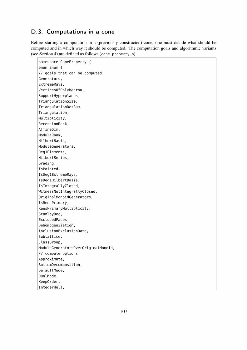
D.3. Computations in a cone

Before starting a computation in a (previously constructed) cone, one must decide what should becomputed and in which way it should be computed. The computation goals and algorithmic variants(see Section 4) are defined as follows (cone_property.h):

namespace ConeProperty {

enum Enum {

// goals that can be computed

Generators,

ExtremeRays,

VerticesOfPolyhedron,

SupportHyperplanes,

TriangulationSize,

TriangulationDetSum,

Triangulation,

Multiplicity,

RecessionRank,

AffineDim,

ModuleRank,

HilbertBasis,

ModuleGenerators,

Deg1Elements,

HilbertSeries,

Grading,

IsPointed,

IsDeg1ExtremeRays,

IsDeg1HilbertBasis,

IsIntegrallyClosed,

WitnessNotIntegrallyClosed,

OriginalMonoidGenerators,

IsReesPrimary,

ReesPrimaryMultiplicity,

StanleyDec,

ExcludedFaces,

Dehomogenization,

InclusionExclusionData,

Sublattice,

ClassGroup,

ModuleGeneratorsOverOriginalMonoid,

// compute options

Approximate,

BottomDecomposition,

DefaultMode,

DualMode,

KeepOrder,

IntegerHull,

107

MaximalSubspace,

ConeDecomposition,

EnumSize // this has to be the last entry, to get the number of entries in the enum

}; // remember to change also the string conversion function if you change this enum

}

The class ConeProperties is based on this enumeration. Its instantiation are essentially boolean vectorsthat can be accessed via the names in the enumeration. Instantiations of the class are used to setcomputation goals and algorithmic variants and to check whether the goals have been reached.

There exist versions of compute for up to 3 cone properties:

ConeProperties Cone<Integer>::compute(ConeProperty::Enum cp)

ConeProperties Cone<Integer>::compute(ConeProperty::Enum cp1,

ConeProperty::Enum cp2)

ConeProperties Cone<Integer>::compute(ConeProperty::Enum cp1,

ConeProperty::Enum cp2, ConeProperty::Enum cp3)

An example:

MyCone.compute(ConeProperty::HilberBasis, ConeProperty::Multiplicity)

If you want to specify more than 3 cone properties, you can define an instance of ConeProoerties

yourself and call

ConeProperties Cone<Integer>::compute(ConeProperties ToCompute)

An example:

ConeProperties Wanted;

Wanted.set(ConeProperty::Triangulation, ConeProperty::HilbertBasis);

MyCone.compute(Wanted);

All get... functions that are listed in the next section, try to compute the data asked for if they havenot yet been computed. Unless you are interested in more than a single result, we recommend touse compute since the data asked for can then be computed in a single run. For example, if theHilbert basis and the multiplicity are wanted, then it would be a bad idea to call getHilbertBasisand getMultiplicity consecutively.

Please inspect cone_property.cpp for the full list of methods implemented in the class ConeProperties.Here we only mention the constructors

ConeProperties::ConeProperties(ConeProperty::Enum p1)

ConeProperties::ConeProperties(ConeProperty::Enum p1, ConeProperty::Enum p2)

ConeProperties::ConeProperties(ConeProperty::Enum p1, ConeProperty::Enum p2,

ConeProperty::Enum p3)

and the functions

108

ConeProperties& ConeProperties::set(ConeProperty::Enum p1, bool value)

ConeProperties& ConeProperties::set(ConeProperty::Enum p1, ConeProperty::Enum p2)

bool ConeProperties::test(ConeProperty::Enum Property) const

The return value of compute can be used to check whether the computation goals have been reached:the reached goals are set to false, and the “surviving” ones are those that have not been reached. Butthere is a more explicit way to do this that we will explain in the next section.

A string can be converted to a cone property and conversely:

ConeProperty::Enum toConeProperty(const string&)

const string& toString(ConeProperty::Enum)

D.4. Retrieving results

As remarked above, all get... functions that are listed below, try to compute the data asked for if theyhave not yet been computed.

The functions that return a matrix encoded as vector<vector<Integer> > have variants that return amatrix encoded in the libnormaliz class Matrix<Integer>. These are not listed below; see cone.h.

D.4.1. Checking computations

In order to check whether a computation goal has been reached, one can use

bool Cone<Integer>::isComputed(ConeProperty::Enum prop) const

for example

bool done=MyCone.isComputed(ConeProperty::HilbertBasis)

D.4.2. Rank, index and dimension

size_t getEmbeddingDim()

size_t Cone<Integer>::getRank()

Integer Cone<Integer>::getIndex()

Integer Cone<Integer>::getUnitGroupIndex()

size_t Cone<Integer>::getRecessionRank()

long Cone<Integer>::getAffineDim()

size_t Cone<Integer>::getModuleRank()

The function getIndex() returns the internal index which is only defined if original generators aredefined. See Section D.4.13 for the external index.

109

The last three functions return values that are only well-defined after inhomogeneous computations.

D.4.3. Support hyperplanes and constraints

const vector< vector<Integer> >& Cone<Integer>::getSupportHyperplanes()

size_t Cone<Integer>::getNrSupportHyperplanes()

The first function returns the support hyperplanes of the (homogenized) cone. The second functionreturns the number of support hyperplanes.

Together with the equations and congruences the support hyperplanes can also be accessed by

map< InputType , vector< vector<Integer> > > Cone<Integer>::getConstraints ()

The map returned contains three pairs whose keys are

Type::inequalities

Type::equations

Type::congruences

D.4.4. Extreme rays and vertices

const vector< vector<Integer> >& Cone<Integer>::getExtremeRays()

size_t Cone<Integer>::getNrExtremeRays()

const vector< vector<Integer> >& Cone<Integer>::getVerticesOfPolyhedron()

size_t Cone<Integer>::getNrVerticesOfPolyhedron()

In the inhomogeneous case the first function returns the extreme rays of the recession cone, and thesecond the vertices of the polyhedron. (Together they form the extreme rays of the homogenized cone.)

D.4.5. Generators

const vector< vector<Integer> >& Cone<Integer>::getOriginalMonoidGenerators()

size_t Cone<Integer>::getNrOriginalMonoidGenerators()

Note that original generators are not always defined. The system of generators of the cone that is usedin the computations and its cardinality are returned by

const vector< vector<Integer> >& Cone<Integer>::getGenerators()

size_t Cone<Integer>::getNrGenerators()

D.4.6. Lattice points in polytopes and elements of degree 1

const vector< vector<Integer> >& Cone<Integer>::getDeg1Elements()

size_t Cone<Integer>::getNrDeg1Elements()

110

D.4.7. Hilbert basis

In the nonpointed case we need the maximal linear subspace of the cone:

const vector< vector<Integer> >& Cone<Integer>::getMaximalSubspace()

size_t Cone<Integer>::getDimMaximalSubspace()

One of the prime results of Normaliz and its cardinality are returned by

const vector< vector<Integer> >& Cone<Integer>::getHilbertBasis()

size_t Cone<Integer>::getNrHilbertBasis()

Inhomogeneous case the functions refer to the the Hilbert basis of the recession cone. The modulegeneraors of the lattice points in the polyhedron are accessed by

const vector< vector<Integer> >& Cone<Integer>::getModuleGenerators()

size_t Cone<Integer>::getNrModuleGenerators()

D.4.8. Module generators over original monoid

const vector< vector<Integer> >&

Cone<Integer>::getModuleGeneratorsOverOriginalMonoid()

size_t Cone<Integer>::getNrModuleGeneratorsOverOriginalMonoid()

D.4.9. Grading and dehomogenization

vector<Integer> Cone<Integer>::getGrading()

Integer Cone<Integer>::getGradingDenom()

The second function returns the denominator of the grading.

vector<Integer> Cone<Integer>::getDehomogenization()

D.4.10. Enumerative data

mpq_class Cone<Integer>::getMultiplicity()

Don’t forget that the multiplicity is measured by a rational, not necessarily integral polytope. Thereforeit need not be an integer.

The Hilbert series is stored in a class of its own. It is retrieved by

const HilbertSeries& Cone<Integer>::getHilbertSeries()

It contains several data fields that can be accessed as follows (see hilbert_series.h):

const vector<mpz_class>& getNum() const;

const map<long, denom_t>& getDenom() const;

111

const vector<mpz_class>& getCyclotomicNum() const;

const map<long, denom_t>& getCyclotomicDenom() const;

long getDegreeAsRationalFunction() const;

long getShift() const;

bool isHilbertQuasiPolynomialComputed() const;

vector< vector<mpz_class> > getHilbertQuasiPolynomial() const;

long getPeriod() const;

mpz_class getHilbertQuasiPolynomialDenom() const;

The first four functions refer to two representations of the Hilbert series as a rational function in thevariable t: the first has a denominator that is a product of polynomials (1− tg)e, the second has adenominator that is a product of cylotomic polynomials. In both cases the numerators are given bytheir coefficient vectors, and the denominators are lists of pairs (g,e) where in the second case g is theorder of the cyclotomic polynomial.

The degree as a rational function is of course independent of the chosen representation, but may benegative, as well as the shift that indicates with which power of t the numerator tarts. >since thedenominator has a nonzero constant term in both cases, this is exactly the smallest degree in which theHilbert function has a nonzero value.

The Hilbert quasipolynomial is represented by a vector whose length is the period and whose entries areitself vectors that represent the coefficients of the individual polynomials corresponding to the residueclasses modulo the period. These integers must be divided by the common denominator that is returnedby the last function.

For the input type rees_algebra we provide

Integer Cone<Integer>::getReesPrimaryMultiplicity()

D.4.11. Triangulation and disjoint decomposition

The triangulation, the size and the sum of the determinants are returned by

const vector< pair<vector<key_t>,Integer> >& Cone<Integer>::getTriangulation()

size_t Cone<Integer>::getTriangulationSize()

Integer Cone<Integer>::getTriangulationDetSum()

See Section 6.7 for the interpretation of these data. The first component of the pair is the vector ofindices of the simplicial cones in the triangulation. Note that the indices are here counted from 0(whereas they start from 1 in the tri file). The second component is the determinant.

The type of triangulation can be retrieved by

bool Cone<Integer>::isTriangulationNested()

bool Cone<Integer>::isTriangulationPartial()

If the disjoint decomposition has been computed, one gets the 0/1 vectors describing the facets to beremoved

112

const vector<vector<bool> >& Cone<Integer>::getOpenFacets()

D.4.12. Stanley decomposition

The Stanley decomposition is stored in a list whose entries correspond to the simplicial cones in thetriangulation:

const list< STANLEYDATA<Integer> >& Cone<Integer>::getStanleyDec()

Each entry is a record of type STANLEYDATA defined as follows:

struct STANLEYDATA {

vector<key_t> key;

Matrix<Integer> offsets;

};

The key has the same interpretation as for the triangulation, namely as the vector of indices of thegenerators of the simplicial cone (counted from 0). The matrix contains the coordinate vectors of theoffsets of the components of the decomposition that belong to the simplicial cone defined by the key.See Section 6.8 for the interpretation. The format of the matrix can be accessed by the followingfunctions of class Matrix<Integer>:

size_t nr_of_rows() const

size_t nr_of_columns() const

The entries are accessed in the same way as those of vector<vector<Integer> >.

D.4.13. Coordinate transformation

The coordinate transformation from the ambient lattice to the sublattice generated by the Hilbert basisand the basis of the maximal subspace can be returned as follows:

const Sublattice_Representation<Integer>& Cone<Integer>::getSublattice()

An object of type Sublattice_Representation models a sequence of Z-homomorphisms

Zr ϕ−→ Zn π−→ Zr

with the following property: there exists c ∈ Z, c 6= 0, such that π ◦ϕ = c · idZr . In particular ϕ isinjective. One should view the two maps as a pair of coordinate transformations: ϕ is determined bya choice of basis in the sublattice U = ϕ(Zr), and it allows us to transfer vectors from U ∼= Zr to theambient lattice Zn. The map π is used to realize vectors from U as linear combinations of the givenbasis of U ∼= Zr: after the application of π one divides by c. (If U is a direct summand of Zn, one canchoose c = 1, and conversely.) Normaliz considers vectors as rows of matrices. Therefore ϕ is givenas an r×n-matrix and π is given as an n× r matrix.

The data just described can be accessed as follows (sublattice_representation.h):

113

const vector<vector<Integer> >& getEmbedding() const

const vector<vector<Integer> >& getProjection() const

Integer getAnnihilator() const

Here “Embedding” refers to ϕ and “Projection” to π (though π is not always surjective). The “Annihi-lator” is the number c above. (It annihilates Zr modulo π(Zn).)

The numbers n and r are accessed in this order by

size_t getDim() const

size_t getRank() const

The external index, namely the order of the torsion subgroup of Zn/U , is returned by

mpz_class getExternalIndex() const

Very often ϕ and ψ are identity maps, and this property can be tested by

bool IsIdentity()const

The constraints computed by Normaliz are “hidden” in the sublattice representation. They van beaccessed by

const vector<vector<Integer> >& getEquations() const

const vector<vector<Integer> >& getCongruences() const

D.4.14. Class group

vector<Integer> Cone<Integer>::getClassGroup()

The return value is to be interpreted as follows: The entry for index 0 is the rank of the class group.The remaining entries contain the orders of the summands in a direct sum decomposition of the torsionsubgroup.

D.4.15. Integer hull

For the computation of the integer hull an auxiliary cone is constructed. A reference to it is returned by

Cone<Integer>& Cone<Integer>::getIntegerHullCone() const

For example, the support hyperplanes of the integer hull can be accessed by

MyCone.getIntegerHullCone().getSupportHyperplanes()

D.4.16. Excluded faces

Before using the excluded faces Normaliz makes the collection irredundant by discarding those thatare contained in others. The irredundant collection (given by hyperplanes that intersect the cone in the

114

faces) and its cardinality are returned by

const vector< vector<Integer> >& Cone<Integer>::getExcludedFaces()

size_t Cone<Integer>::getNrExcludedFaces()

For the computation of the Hilbert series the all intersections of the excluded faces are computed, andfor each resulting face the weight with which it must be counted is computed. These data can beaccessed by

const vector< pair<vector<key_t>,long> >&

Cone<Integer>::getInclusionExclusionData()

The first component of each pair contains the indices of the generators that lie in the face and the secondcomponent is the weight.

D.4.17. Boolean valued results

All the “questions” to the cone that can be asked by the boolean valued functions in this section start acomputation if the answer is not yet known.

The first, The question

bool Cone<Integer>::isIntegrallyClosed()

does not trigger a computation of the full Hilbert basis. The computation stops as soon as the answercan be given, and this is the case when an element in the integral closure has been found that is not inthe original monoid. Such an element is retrieved by

vector<Integer> Cone<Integer>::getWitnessNotIntegrallyClosed()

As discussed in Section 6.6.3 it can sometimes be useful to ask

bool Cone<Integer>::isPointed()

before a more complex computation is started.

The next two functions answer the question whether the Hilbert basis or at least the extreme rays livein degree 1.

bool Cone<Integer>::isDeg1ExtremeRays()

bool Cone<Integer>::isDeg1HilbertBasis()

Finally we have

bool Cone<Integer>::isInhomogeneous()

bool Cone<Integer>::isReesPrimary()

isReesPrimary() checks whether the ideal defining the Rees algebra is primary to the irrelevant max-imal ideal.

115

D.5. Exception handling

All exceptions that are thrown in libnormaliz are derived from the abstract class NormalizExceptionthat itself is derived from std::exception:

class NormalizException: public std::exception

The following exceptions must be caught by the calling program:

class ArithmeticException: public NormalizException

class BadInputException: public NormalizException

class NotComputableException: public NormalizException

class FatalException: public NormalizException

The ArithmeticException is leaves libnormaliz if a nonrecoverable overflow occurs (it is also usedinternally for the change of integer type). This should not happen for cones of integer type mpz_class,unless it is caused by a bug in the program. The BadInputException is thrown whenever the input isinconsistent; the reasons for this are manifold. The NotComputableException is thrown if a computa-tion goal cannot be reached. The FatalException should never appear. It covers error situations thatcan only be caused by a bug in the program. At many places libnormaliz has assert verificationsbuilt in that serve the same purpose.

There are two more exceptions for the communication within libnormaliz that should not leave it:

class NonpointedException: public NormalizException

class NotIntegrallyClosedException: public NormalizException

D.6. Control of output

By using

bool setVerboseDefault(bool v)

one can control the verbose output of libnormaliz. The default value is false. This is a global settingthat effects all cones constructed afterwards. However, for every cone one can set an individual valueof verbose by

bool Cone<Integer>::setVerbose(bool v)

Both functions return the previous value.

The default values of verbose output and error output are std::cout and std::cerr. These values canbe changed by

void setVerboseOutput(std::ostream&)

void setErrorOutput(std::ostream&)

116

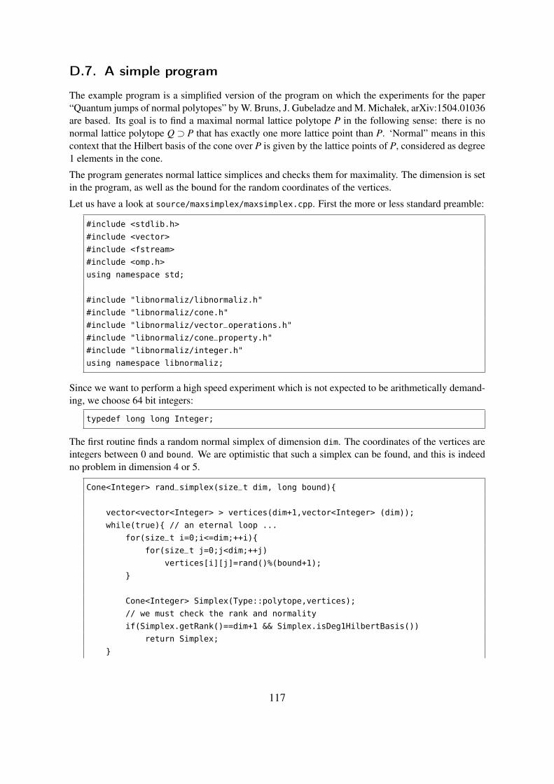
D.7. A simple program

The example program is a simplified version of the program on which the experiments for the paper“Quantum jumps of normal polytopes” by W. Bruns, J. Gubeladze and M. Michałek, arXiv:1504.01036are based. Its goal is to find a maximal normal lattice polytope P in the following sense: there is nonormal lattice polytope Q ⊃ P that has exactly one more lattice point than P. ‘Normal” means in thiscontext that the Hilbert basis of the cone over P is given by the lattice points of P, considered as degree1 elements in the cone.

The program generates normal lattice simplices and checks them for maximality. The dimension is setin the program, as well as the bound for the random coordinates of the vertices.

Let us have a look at source/maxsimplex/maxsimplex.cpp. First the more or less standard preamble:

#include <stdlib.h>

#include <vector>

#include <fstream>

#include <omp.h>

using namespace std;

#include "libnormaliz/libnormaliz.h"

#include "libnormaliz/cone.h"

#include "libnormaliz/vector_operations.h"

#include "libnormaliz/cone_property.h"

#include "libnormaliz/integer.h"

using namespace libnormaliz;

Since we want to perform a high speed experiment which is not expected to be arithmetically demand-ing, we choose 64 bit integers:

typedef long long Integer;

The first routine finds a random normal simplex of dimension dim. The coordinates of the vertices areintegers between 0 and bound. We are optimistic that such a simplex can be found, and this is indeedno problem in dimension 4 or 5.

Cone<Integer> rand_simplex(size_t dim, long bound){

vector<vector<Integer> > vertices(dim+1,vector<Integer> (dim));

while(true){ // an eternal loop ...

for(size_t i=0;i<=dim;++i){

for(size_t j=0;j<dim;++j)

vertices[i][j]=rand()%(bound+1);

}

Cone<Integer> Simplex(Type::polytope,vertices);

// we must check the rank and normality

if(Simplex.getRank()==dim+1 && Simplex.isDeg1HilbertBasis())

return Simplex;

}

117

vector<vector<Integer> > dummy_gen(1,vector<Integer>(1,1));

// to make the compiler happy

return Cone<Integer>(Type::cone,dummy_gen);

}

We are looking for a normal polytope Q ⊃ P with exactly one more lattice point. The potential extralattice points z are contained in the matrix jump_cands. There are two obstructions for Q = conv(P,z)to be tested: (i) z is the only extra lattice point and (ii) Q is normal. It makes sense to test them in thisorder since most of the time condition (i) is already violated and it is much faster to test.

bool exists_jump_over(Cone<Integer>& Polytope,

const vector<vector<Integer> >& jump_cands){

vector<vector<Integer> > test_polytope=Polytope.getExtremeRays();

test_polytope.resize(test_polytope.size()+1);

for(size_t i=0;i<jump_cands.size();++i){

test_polytope[test_polytope.size()-1]=jump_cands[i];

Cone<Integer> TestCone(Type::cone,test_polytope);

if(TestCone.getNrDeg1Elements()!=Polytope.getNrDeg1Elements()+1)

continue;

if(TestCone.isDeg1HilbertBasis())

return true;

}

return false;

}

In order to make the (final) list of candidates z as above we must compute the widths of P over itssupport hyperplanes.

vector<Integer> lattice_widths(Cone<Integer>& Polytope){

if(!Polytope.isDeg1ExtremeRays()){

cerr<< "Cone in lattice_widths is not defined by lattice polytope"<< endl;

exit(1);

}

vector<Integer> widths(Polytope.getNrExtremeRays(),0);

for(size_t i=0;i<Polytope.getNrSupportHyperplanes();++i){

for(size_t j=0;j<Polytope.getNrExtremeRays();++j){

// v_scalar_product is a useful function from vector_operations.h

Integer test=v_scalar_product(Polytope.getSupportHyperplanes()[i],

Polytope.getExtremeRays()[j]);

if(test>widths[i])

widths[i]=test;

}

}

return widths;

}

118

int main(int argc, char* argv[]){

time_t ticks;

srand(time(&ticks));

cout << "Seed " <<ticks << endl; // we may want to reproduce the run

size_t polytope_dim=4;

size_t cone_dim=polytope_dim+1;

long bound=6;

vector<Integer> grading(cone_dim,0);

// at some points we need the explicit grading

grading[polytope_dim]=1;

size_t nr_simplex=0; // for the progress report

Since the computations are rather small, we suppress parallelization (except for one step below).

while(true){

omp_set_num_threads(1);

Cone<Integer> Candidate=rand_simplex(polytope_dim,bound);

nr_simplex++;

if(nr_simplex%1000 ==0)

cout << "simplex " << nr_simplex << endl;

Maximality is tested in 3 steps. Most often there exists a lattice point z of height 1 over P. If so, thenconv(P,z) contains only z as an extra lattice point and it is automatically normal. In order to find sucha point we must move the support hyperplanes outward by lattice distance 1.

vector<vector<Integer> > supp_hyps_moved=Candidate.getSupportHyperplanes();

for(size_t i=0;i<supp_hyps_moved.size();++i)

supp_hyps_moved[i][polytope_dim]+=1;

Cone<Integer> Candidate1(Type::inequalities,supp_hyps_moved,

Type::grading,to_matrix(grading));

if(Candidate1.getNrDeg1Elements()>Candidate.getNrDeg1Elements())

continue; // there exists a point of height 1

Among the polytopes that have survived the height 1 test, most nevertheless have suitable points z closeto them, and it makes sense not to use the maximum possible height immediately. Note that we mustnow test normality explicitly.

cout << "No ht 1 jump"<< " #latt " << Candidate.getNrDeg1Elements() << endl;

// move the hyperplanes further outward


supp_hyps_moved[i][polytope_dim]+=polytope_dim;

Cone<Integer> Candidate2(Type::inequalities,supp_hyps_moved,

119

Type::grading,to_matrix(grading));

cout << "Testing " << Candidate2.getNrDeg1Elements()

<< " jump candidates" << endl; // including the lattice points in P

if(exists_jump_over(Candidate,Candidate2.getDeg1Elements()))

continue;

Now we can be optimistic that a maximal polytope P has been found, and we test all candidates z thatsatisfy the maximum possible bound on their lattice distance to P.

cout << "No ht <= 1+dim jump" << endl;

vector<Integer> widths=lattice_widths(Candidate);


supp_hyps_moved[i][polytope_dim]+=

-polytope_dim+(widths[i])*(polytope_dim-2);

The computation may become arithmetically critical at this point. Therefore we use mpz_class for ourcone. The conversion to and from mpz_class is done by routines contained in convert.h.

vector<vector<mpz_class> > mpz_supp_hyps;

convert(mpz_supp_hyps,supp_hyps_moved);

vector<mpz_class> mpz_grading=convertTo<vector<mpz_class> >(grading);

The computation may need some time now. Therefore we allow a little bit of parallelization.

omp_set_num_threads(4);

Since P doesn’t have many vertices (even if we use these routines for more general polytopes thansimplices), we don’t expect too many vertices for the enlarged polytope. In this situation it makessense to set the algorithmic variant Approximate.

Cone<mpz_class> Candidate3(Type::inequalities,mpz_supp_hyps,

Type::grading,to_matrix(mpz_grading));

Candidate3.compute(ConeProperty::Deg1Elements,ConeProperty::Approximate);

vector<vector<Integer> > jumps_cand; // for conversion from mpz_class

convert(jumps_cand,Candidate3.getDeg1Elements());

cout << "Testing " << jumps_cand.size() << " jump candidates" << endl;

if(exists_jump_over(Candidate, jumps_cand))

continue;

Success!

cout << "Maximal simplex found" << endl;

cout << "Vertices" << endl;

Candidate.getExtremeRaysMatrix().pretty_print(cout); // a goody from matrix.h

cout << "Number of lattice points = " << Candidate.getNrDeg1Elements();

cout << " Multiplicity = " << Candidate.getMultiplicity() << endl;

} // end while

} // end main

120

For the compilation of maxsimplex.cpp we have added a Makefile. Running the program needs a littlebit of patience. However, within a few hours a maximal simplex should have emerged. From a log file:

simplex 143000

No ht 1 jump #latt 9

Testing 22 jump candidates





No ht <= 1+dim jump


Maximal simplex found

Vertices

1 3 5 3 1

2 3 0 3 1

3 0 5 5 1

5 2 2 1 1

6 5 6 2 1

Number of lattice points = 29 Multiplicity = 275

References

[1] T. Achterberg. SCIP: Solving constraint integer programs. Mathematical Programming Compu-tation 1 (2009), 1–41. Available from http://mpc.zib.de/index.php/MPC/article/view/4

[2] V. Almendra and B. Ichim. jNormaliz 1.7. Available at http://normaliz.uos.de

[3] V. Baldoni, N. Berline, J.A. De Loera, B. Dutra, M. Köppe, S. Moreinis, G. Pinto, M. Vergne,J. Wu, A User’s Guide for LattE integrale v1.7.2, 2013. Software package LattE is available athttp://www.math.ucdavis.edu/~latte/

[4] W. Bruns and J. Gubeladze. Polytopes, rings, and K-theory. Springer 2009.

[5] W. Bruns, R. Hemmecke, B. Ichim, M. Köppe and C. Söger. Challenging computations ofHilbert bases of cones associated with algebraic statistics . Exp. Math.20 (2011), 25–33.

[6] W. Bruns and J. Herzog. Cohen-Macaulay rings. Rev. ed. Cambridge University Press 1998.

[7] W. Bruns and B. Ichim. Normaliz: algorithms for rational cones and affine monoids. J. Algebra324 (2010) 1098–1113.

[8] W. Bruns, B. Ichim and C. Söger. The power of pyramid decompositions in Normaliz. J. Symb.Comp., to appear. Preprint arXiv:1206.1916.

[9] W .Bruns and R. Koch. Computing the integral closure of an affine semigroup. Univ. Iagell. ActaMath. 39 (2001), 59–70.

[10] W. Bruns and C. Söger. The computation of generalized Ehrhart series in Normaliz. J. Symb.Comp. 68 (2015), 75–86.

[11] W. Bruns and C. Söger. NmzIntegrate 1.3. Available at http://normaliz.uos.de

121

http://mpc.zib.de/index.php/MPC/article/view/4


http://www.math.ucdavis.edu/~latte/


[12] S. Gutsche, M. Horn, C. Söger, NormalizInterface for GAP. Available at https://github.com/gap-packages/NormalizInterface.

[13] M. Köppe and S. Verdoolaege. Computing parametric rational generating functions with a pri-mal Barvinok algorithm. Electron. J. Comb. 15, No. 1, Research Paper R16, 19 p. (2008).

[14] L. Pottier. The Euclide algorithm in dimension n. Research report, ISSAC 96, ACM Press 1996.

122

https://github.com/gap-packages/NormalizInterface

https://github.com/gap-packages/NormalizInterface

Documents

Normaliz 3.1