Embed Size (px)
Citation preview
1
Marshall Alan Rogers-Martinez Department of Applied Physics and Applied Mathematics
Columbia University, New York, New York
Image Credit: Lola Jusidman
The Dynamics of Normal Faulting at Mid-Ocean Ridges
2
The Dynamics of Normal Faulting at Mid-Ocean Ridges
M. A. Rogers-Martinez1 1Department of Applied Physics and Applied Mathematics, Columbia University, New York, NY 10027
I. ABSTRACT In this paper we wish to explore the relation between the
energy release (specifically the moment magnitude, MW) of earthquakes at mid-ocean ridges, the maximum stress σ22 in the direction along strike and the size of the physical fault plane. Understanding such dynamics may eventually provide better insight into the production of new seafloor near axial magma chambers (AMC), as coseismic changes in tensile stress are believed to be instrumental in dike formation near AMCs, leading to the eventual production of new seafloor.
II. INTRODUCTION
To model our various deformation scenarios, the open-source program RELAX was used. RELAX evaluates the displacement and stress in a half space with gravity due to dislocations, Mogi sources, and surface traction. For the purposes of this paper, dislocations along discrete normal fault planes were used to simulate the stress environment.
Several approximations were made in order to run the computationally intensive simulations more smoothly. First, we assume a standard dip angle of 60°. However, as was shown by [Lavier et al., 1999], in order to obtain a large-offset low-angle normal fault, a relatively thin and cohesive brittle layer is required. Although our simulations are only concerned with the first several kilometers of oceanic brittle crust, the offsets used are on the order of millimeters to centimeters. Secondly, we assume an isotropic medium as our oceanic crust. However, it has been shown [Behn et al., 2002] that the Young’s modulus and yield strength of oceanic crust near spreading ridges varies somewhat with depth. As such, our assumption of an isotropic homogenous medium for fracture and seismic propagation may not provide realistic insight into coseismic stress states near normal faults along spreading ridges. Our third assumption is that slip is uniform along the fault, i.e. there is perfect shear. Because we are concerned with low energy earthquakes with small amounts of slip, such an approximation is likely admissible.
III. BACKGROUND A. GREEN’S FUNCTION AND THEORY1
RELAX solves the displacement field for static deformation in a three-dimensional half space using the elastic Green’s function. Consider the following Navier-Lamé equation for displacement:
µ !1!!
uj,ij + ui,ij"#$
%&' + fi = 0 (1)
where µ is the shear modulus, ui is the displacement, fi is the internal body force and α is a dimensionless parameter that can be expressed in terms of Lamé’s parameter λ or Poisson’s ratio ν:
! = " + µ" + 2µ
= 12 1!#( )
(2)
The boundary condition for this system of equations is:
qi +! ijn j + !"gu3ni = 0 , x3 = 0 (3)
where σij is the Cauchy stress tensor, qi is the surface traction, ρ is the density and ni is the vector normal to the surface, (0,0,-1). The solution displacement that satisfies (1) and (3) can be decomposed into both a particular and homogenous contribution:
ui = uih + ui
p (4) where the homogenous displacement field is a solution of the homogenous Navier’s equation with inhomogeneous boundary conditions:
!uj,ijh + (1!! )ui, jj
h = 0 (5)
The particular solution however satisfies (1) regardless of any inhomogeneous surface boundary conditions. The particular solution can be found in the Fourier domain as:
uip(k1,k2,k3) =
0, k1 = k2 = k3 = 01µ(1!! )klkl! ij !!kik j
4! 2 (klkl )2 f j, otherwise
"
#$
%$
(6)
where ki are the wavenumbers and the hats correspond to the Fourier transform of that variable.
It should be noted that the zero wavenumber component of the Fourier transform corresponds to a rigid-body displacement rather than an elastic deformation. The temporary solution requires a large correction to satisfy the boundary condition. However, these corrections are not particularly elucidating and the complete theoretical background regarding how RELAX solves for the displacement field in a three-dimensional half space can be found in the user manual [Barbot, 2011].
B. PHYSICAL OBSERVATIONS
In order to run meaningful simulations using RELAX we need both appropriate elastic moduli as well as a constraint on fault depth.
According to [Huang and Solomon, 1988], well-determined centroid depths of large ridge-axis earthquakes range from 1 to 6 km beneath the seafloor. That same paper determined that ill-defined centroid depths indicate the beginning of the brittle-ductile transition along spreading ridges. It was also found that for faster spreading rates, the maximum depth of well-defined centroids tended to decrease.
According to [Tolstoy et al., 2006], most on-axis seismicity is too small to be recorded by global seismic networks or regional hydrophone arrays. After deploying ocean bottom seismometers along a segment of the East Pacific Rise, it was found that the majority of the microseismicity on spreading ridges was concentrated at depths ~ .9 -1.4 km [Stroup et al., 2007].
For this short study we have limited the depth of the bottom of our fault plane to 1 km on the presumption that sufficient stresses exist in the upper brittle layer near spreading ridges to induce smaller magnitude earthquakes as well as the anecdotal evidence provided by [Stroup et al., 2007].
C. MATERIAL PROPERTIES
According to the results of a deep sea-drilling project2 concerned with volcanic breccias and basalts, a wide range of elastic constants were found for oceanic basalts. It has been
3
shown by [Behn et al., 2002] that elastic moduli near mid-ocean ridges are highly variable with depth however our shallow depth constraint of 1 km may act as a control for this phenomenon. The following moduli from a sample of flow basalt were used as input parameters while running RELAX:
Lamé Parameter, λ Shear Modulus, µ
50 GPa 32 GPa Table 1: Elastic moduli used with RELAX
[Christensen et al., 1980]
Because the local magnitude scale used by [Tolstoy et al., 2006] and [Stroup et al., 2007] does not provide for a direct relationship between fault plane size and amount of slip, we have chosen to use the moment magnitude scale, MW. By using this scale, we may control for the approximate energy released by various sized faults. The moment magnitude of an earthquake can easily be calculated as:
MW = 23
log10M0
1 N !m"#$
%&' ( 6.0 (7)
where M0 is the seismic moment of the earthquake. The seismic moment is computed as:
M0 = µAD (8) where µ is the shear modulus of the rock, A is the area of rupture along the fault and D is the average displacement along that area of rupture. For the purposes of this paper, a uniform slip was used, so D may be interpreted as the true displacement along the fault. Using (7) and (8), values for D were generated for faults of width 100 m, 333 m and 1000 m for MW = [0, 1, 2]. All faults that were modeled in this study preserved the same aspect ratio between the length l and width w of the fault such that:
l =10w (9)
D. MODEL GEOMETRY According to two-dimensional Mohr-Coulomb theory, the
optimal dip θ of a normal fault can be roughly approximated as [Buck, 1993]:
! = 45! + 12tan!1 µ f
(10)
where µf is the coefficient of friction between both sides of the fault plane. If we assume µf =.6 for our fault, the dip angle we use for our simulations run with RELAX is 60°.
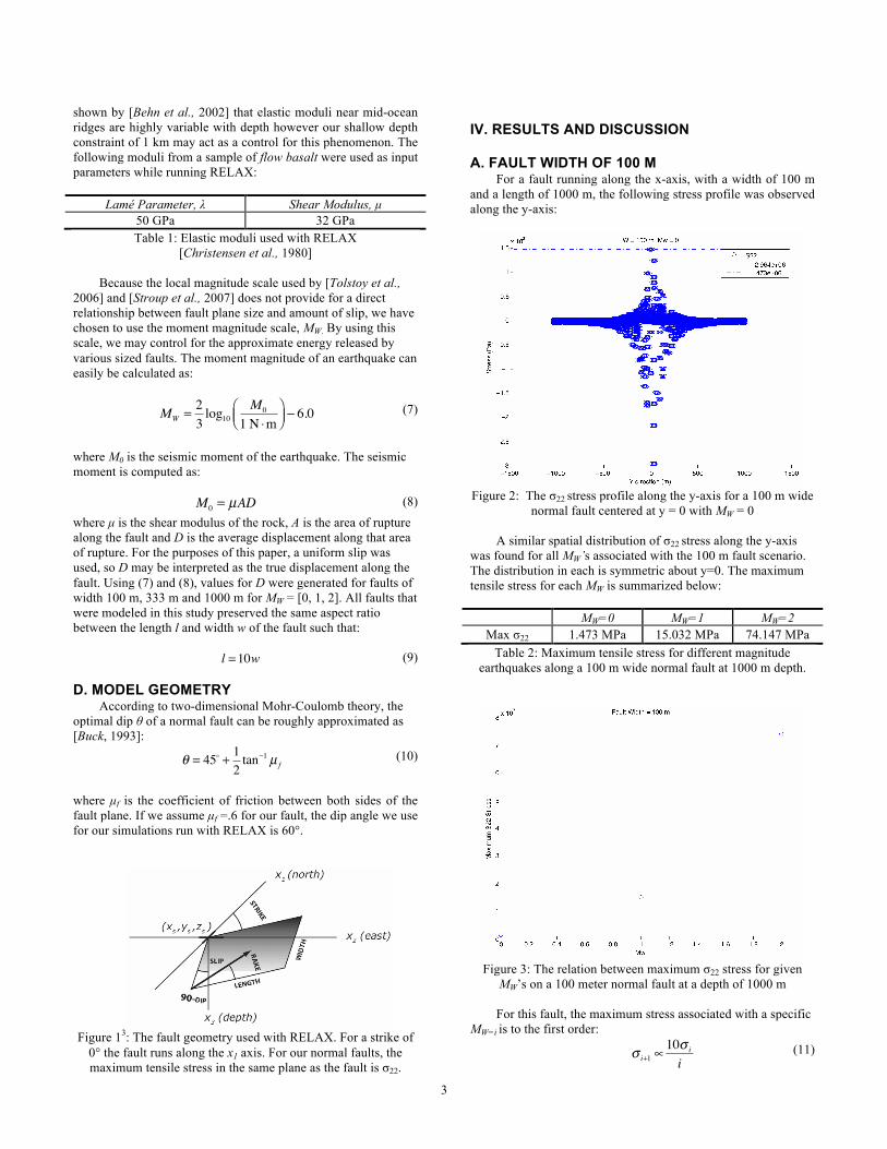
Figure 13: The fault geometry used with RELAX. For a strike of
0° the fault runs along the x1 axis. For our normal faults, the maximum tensile stress in the same plane as the fault is σ22.
IV. RESULTS AND DISCUSSION A. FAULT WIDTH OF 100 M
For a fault running along the x-axis, with a width of 100 m and a length of 1000 m, the following stress profile was observed along the y-axis:
Figure 2: The σ22 stress profile along the y-axis for a 100 m wide
normal fault centered at y = 0 with MW = 0
A similar spatial distribution of σ22 stress along the y-axis was found for all MW’s associated with the 100 m fault scenario. The distribution in each is symmetric about y=0. The maximum tensile stress for each MW is summarized below:
MW=0 MW=1 MW=2
Max σ22 1.473 MPa 15.032 MPa 74.147 MPa Table 2: Maximum tensile stress for different magnitude
earthquakes along a 100 m wide normal fault at 1000 m depth.
Figure 3: The relation between maximum σ22 stress for given
MW’s on a 100 meter normal fault at a depth of 1000 m
For this fault, the maximum stress associated with a specific MW=i is to the first order:
! i+1 !10! i
i (11)
4
Obviously it would have been preferable to have many
thousands of points to conclusively determine this relation, however for the computational resources at hand this was not possible, and only 3 data points were generated.
B. FAULT WIDTH OF 333 M
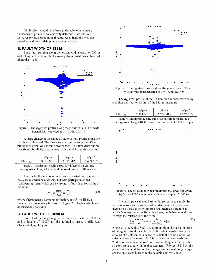
For a fault running along the x-axis, with a width of 333 m and a length of 3330 m, the following stress profile was observed along the y-axis:
Figure 4: The σ22 stress profile along the y-axis for a 333 m wide
normal fault centered at y = 0 with MW = 0
A large change in the shape of the σ22 stress profile along the y-axis was observed. The characteristic symmetric point of the previous distributions became pronounced. This new distribution was found for all MW’s associated with the 333 m fault scenario.
MW=0 MW=1 MW=2
Max σ22 0.696 MPa 3.897 MPa 17.409 MPa Table 3: Maximum tensile stress for different magnitude
earthquakes along a 333 m wide normal fault at 1000 m depth
For this fault, the maximum stress associated with a specific MW=i has a similar relationship, but with perhaps an added “dampening” term which can be thought of as a function of the ith moment:
! i+1 !10! i
i "d= ! i
d(i) (12)
where d represents a damping correction, and d(i) is likely a bounded and increasing function of degree 2 or higher which has absorbed any constants. C. FAULT WIDTH OF 1000 M
For a fault running along the x-axis, with a width of 1000 m and a length of 10000 m, the following stress profile was observed along the y-axis:
Figure 5: The σ22 stress profile along the y-axis for a 1000 m
wide normal fault centered at y = 0 with MW = 0
The σ22 stress profile of the 1000 m fault is characterized by a similar distribution as that of the 333 m long fault.
MW=0 MW=1 MW=2
Max σ22 0.504 MPa 2.529 MPa 14.237 MPa Table 4: Maximum tensile stress for different magnitude
earthquakes along a 1000 m wide normal fault at 1000 m depth
Figure 6: The relation between maximum σ22 stress for given
MW’s on a 1000 meter normal fault at a depth of 1000 m It would appear that as fault width (or perhaps simply the
area) increases, the derivative of the dampening function also increases, so that as the width of a fault increases the rate at which Max σ22 increases for a given magnitude becomes slower. Perhaps the relation is of the form:
limw!"
#d(i,w)#i
= "$ limw!"
#!max
#MW
w( ) = 0 (13)
where w is the width. Such a relation might make sense in terms of energetics. As the width of a fault tends towards infinity, the amount of displacement needed to radiate the same amount of seismic energy decreases. As this distance tends towards the “radius of molecular action” there will no longer be perceivable stresses associated with the displacement [Griffith, 1921]. At this point it is assumed that surface energy and internal body energy are the only contributions to the seismic energy release.
5
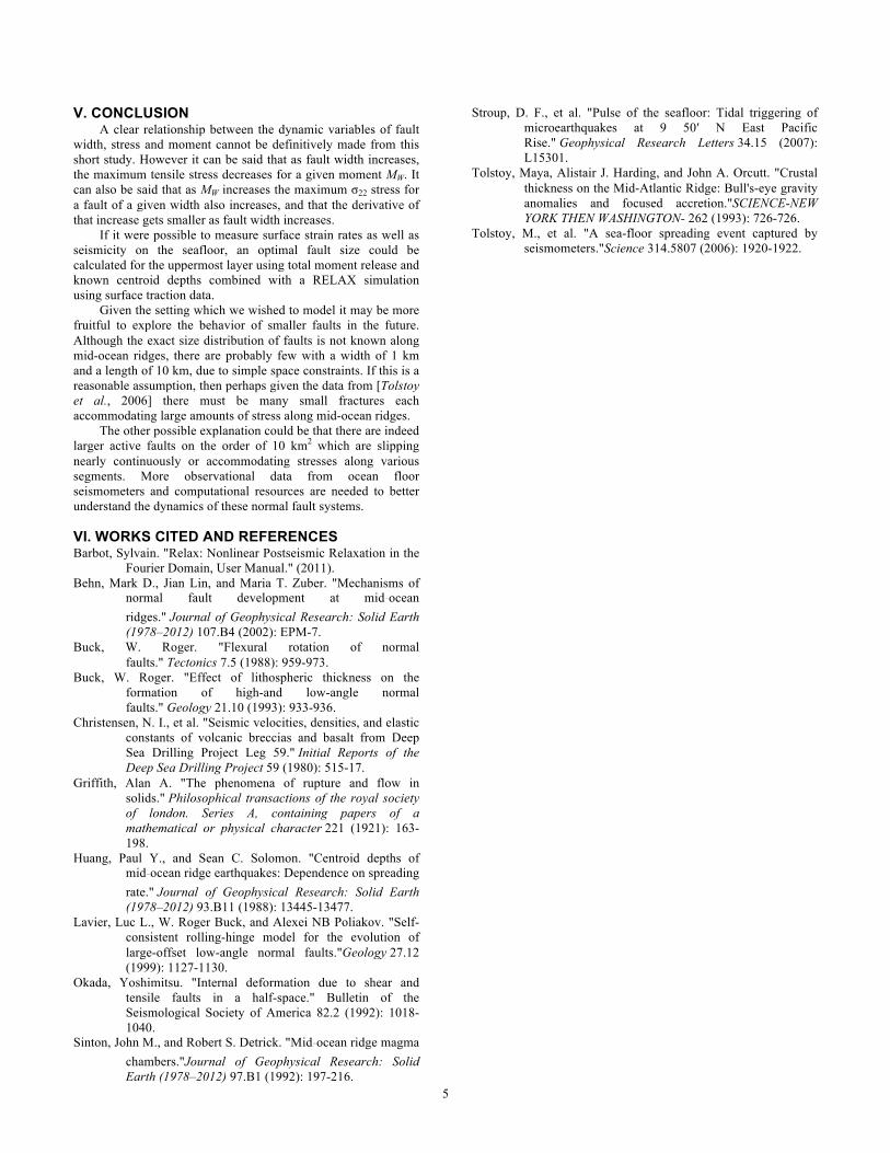
V. CONCLUSION A clear relationship between the dynamic variables of fault
width, stress and moment cannot be definitively made from this short study. However it can be said that as fault width increases, the maximum tensile stress decreases for a given moment MW. It can also be said that as MW increases the maximum σ22 stress for a fault of a given width also increases, and that the derivative of that increase gets smaller as fault width increases.
If it were possible to measure surface strain rates as well as seismicity on the seafloor, an optimal fault size could be calculated for the uppermost layer using total moment release and known centroid depths combined with a RELAX simulation using surface traction data.
Given the setting which we wished to model it may be more fruitful to explore the behavior of smaller faults in the future. Although the exact size distribution of faults is not known along mid-ocean ridges, there are probably few with a width of 1 km and a length of 10 km, due to simple space constraints. If this is a reasonable assumption, then perhaps given the data from [Tolstoy et al., 2006] there must be many small fractures each accommodating large amounts of stress along mid-ocean ridges.
The other possible explanation could be that there are indeed larger active faults on the order of 10 km2 which are slipping nearly continuously or accommodating stresses along various segments. More observational data from ocean floor seismometers and computational resources are needed to better understand the dynamics of these normal fault systems.
VI. WORKS CITED AND REFERENCES Barbot, Sylvain. "Relax: Nonlinear Postseismic Relaxation in the
Fourier Domain, User Manual." (2011). Behn, Mark D., Jian Lin, and Maria T. Zuber. "Mechanisms of
normal fault development at mid‐ocean ridges." Journal of Geophysical Research: Solid Earth (1978–2012) 107.B4 (2002): EPM-7.
Buck, W. Roger. "Flexural rotation of normal faults." Tectonics 7.5 (1988): 959-973.
Buck, W. Roger. "Effect of lithospheric thickness on the formation of high-and low-angle normal faults." Geology 21.10 (1993): 933-936.
Christensen, N. I., et al. "Seismic velocities, densities, and elastic constants of volcanic breccias and basalt from Deep Sea Drilling Project Leg 59." Initial Reports of the Deep Sea Drilling Project 59 (1980): 515-17.
Griffith, Alan A. "The phenomena of rupture and flow in solids." Philosophical transactions of the royal society of london. Series A, containing papers of a mathematical or physical character 221 (1921): 163-198.
Huang, Paul Y., and Sean C. Solomon. "Centroid depths of mid‐ocean ridge earthquakes: Dependence on spreading rate." Journal of Geophysical Research: Solid Earth (1978–2012) 93.B11 (1988): 13445-13477.
Lavier, Luc L., W. Roger Buck, and Alexei NB Poliakov. "Self-consistent rolling-hinge model for the evolution of large-offset low-angle normal faults."Geology 27.12 (1999): 1127-1130.
Okada, Yoshimitsu. "Internal deformation due to shear and tensile faults in a half-space." Bulletin of the Seismological Society of America 82.2 (1992): 1018-1040.
Sinton, John M., and Robert S. Detrick. "Mid‐ocean ridge magma chambers."Journal of Geophysical Research: Solid Earth (1978–2012) 97.B1 (1992): 197-216.
Stroup, D. F., et al. "Pulse of the seafloor: Tidal triggering of microearthquakes at 9 50′ N East Pacific Rise." Geophysical Research Letters 34.15 (2007): L15301.
Tolstoy, Maya, Alistair J. Harding, and John A. Orcutt. "Crustal thickness on the Mid-Atlantic Ridge: Bull's-eye gravity anomalies and focused accretion."SCIENCE-NEW YORK THEN WASHINGTON- 262 (1993): 726-726.
Tolstoy, M., et al. "A sea-floor spreading event captured by seismometers."Science 314.5807 (2006): 1920-1922.
6
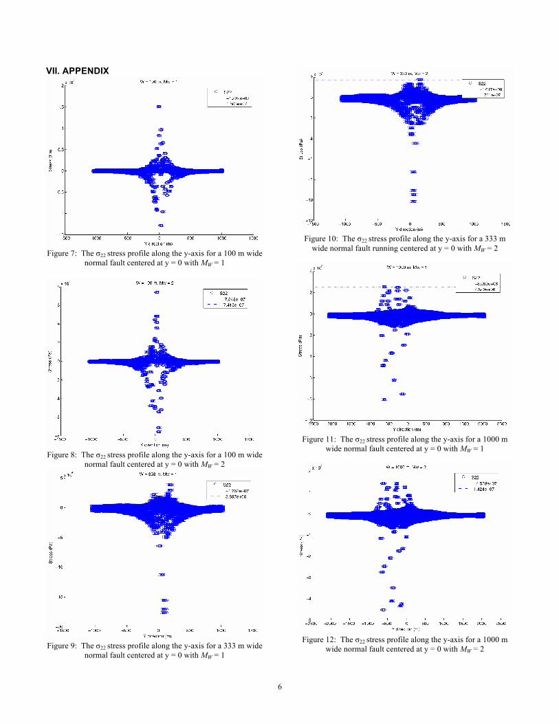
VII. APPENDIX
Figure 7: The σ22 stress profile along the y-axis for a 100 m wide
normal fault centered at y = 0 with MW = 1
Figure 8: The σ22 stress profile along the y-axis for a 100 m wide
normal fault centered at y = 0 with MW = 2
Figure 9: The σ22 stress profile along the y-axis for a 333 m wide
normal fault centered at y = 0 with MW = 1
Figure 10: The σ22 stress profile along the y-axis for a 333 m
wide normal fault running centered at y = 0 with MW = 2
Figure 11: The σ22 stress profile along the y-axis for a 1000 m wide normal fault centered at y = 0 with MW = 1
Figure 12: The σ22 stress profile along the y-axis for a 1000 m
wide normal fault centered at y = 0 with MW = 2
7
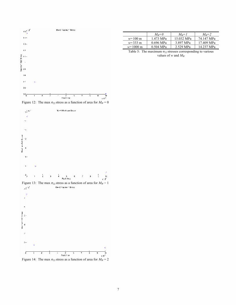
Figure 12: The max σ22 stress as a function of area for MW = 0
Figure 13: The max σ22 stress as a function of area for MW = 1
Figure 14: The max σ22 stress as a function of area for MW = 2
MW=0 MW=1 MW=2
w=100 m 1.473 MPa 15.032 MPa 74.147 MPa w=333 m 0.696 MPa 3.897 MPa 17.409 MPa
w=1000 m 0.504 MPa 2.529 MPa 14.237 MPa Table 5: The maximum σ22 stresses corresponding to various
values of w and MW
8
VIII. ENDNOTES 1 Barbot, Sylvain. "Relax: Nonlinear Postseismic Relaxation in the Fourier Domain, User Manual." (2011). 2 Christensen, N. I., et al. "Seismic velocities, densities, and elastic constants of volcanic breccias and basalt from Deep Sea Drilling Project Leg 59." Initial Reports of the Deep Sea Drilling Project 59 (1980): 515-17. 3 Barbot, Sylvain. "Relax: Nonlinear Postseismic Relaxation in the Fourier Domain, User Manual." (2011).