Embed Size (px)
Citation preview
Nonparametric Statistics

Salad bar, Pizza Hut, China, State of the Art in Structural
Engineering
Learning Objectives
1. Distinguish Parametric & Nonparametric Test Procedures
2. Explain a Variety of Nonparametric Test Procedures
3. Solve Hypothesis Testing Problems Using Nonparametric Tests
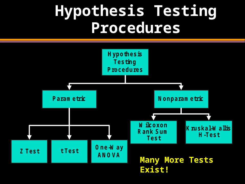
Hypothesis Testing Procedures
HypothesisTesting
Procedures
NonparametricParametric
Z Test
Kruskal-W allisH-Test
W ilcoxonRank Sum
Test
t Test One-W ayANOVA
Many More Tests Exist!
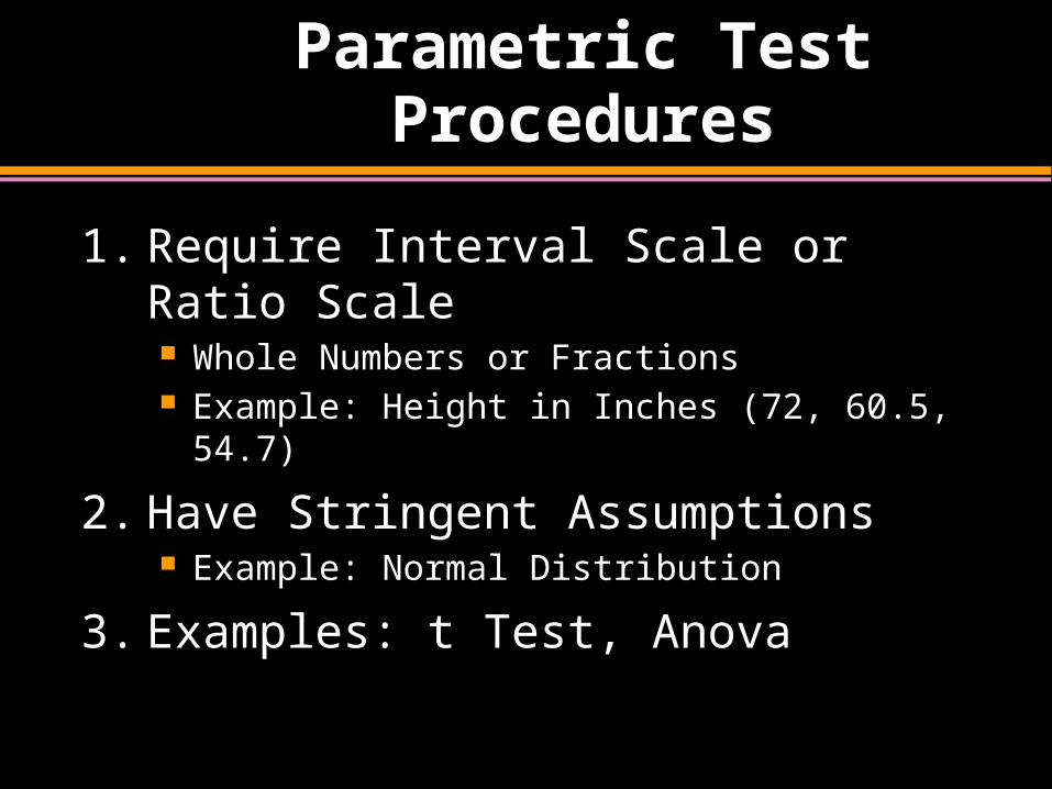
Parametric Test Procedures
1. Require Interval Scale or Ratio Scale Whole Numbers or Fractions Example: Height in Inches (72, 60.5, 54.7)
2. Have Stringent Assumptions Example: Normal Distribution
3. Examples: t Test, Anova
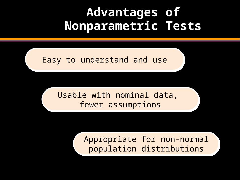
Advantages of Nonparametric Tests
Easy to understand and useEasy to understand and use
Usable with nominal data, fewer assumptions
Usable with nominal data, fewer assumptions
Appropriate for non-normal population distributions
Appropriate for non-normal population distributions
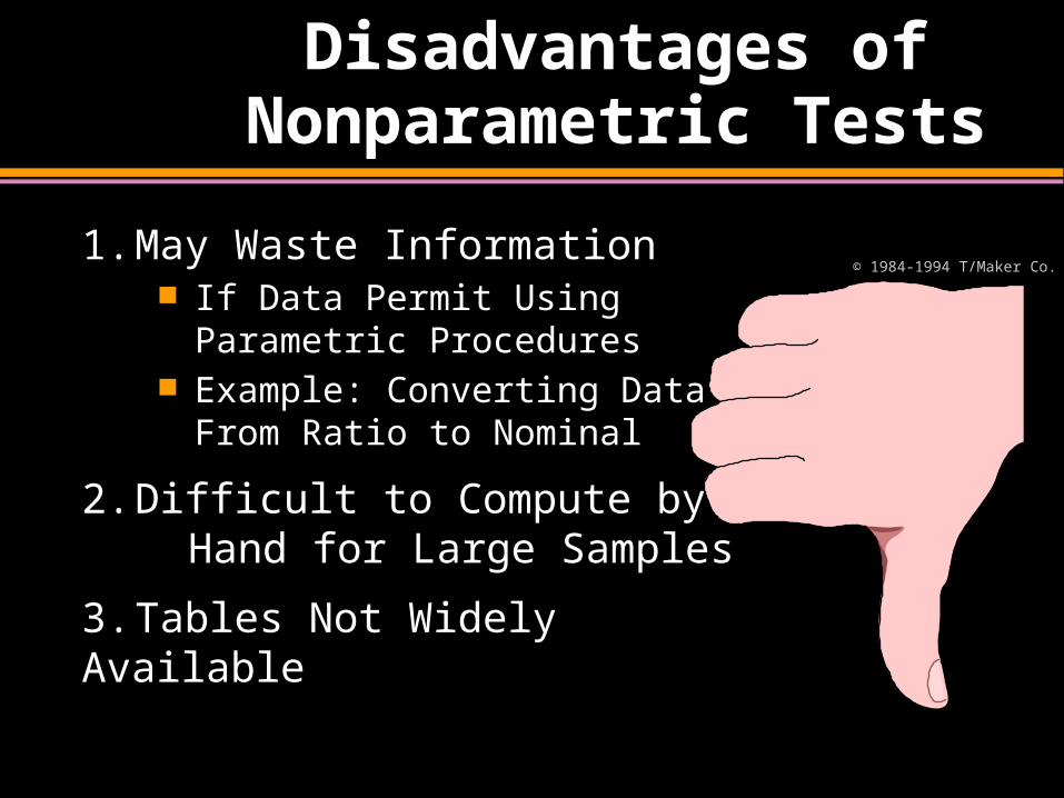
Disadvantages of Nonparametric Tests
1. May Waste Information If Data Permit Using Parametric
Procedures Example: Converting Data From
Ratio to Nominal
2. Difficult to Compute by Hand for Large Samples
3. Tables Not Widely Available
© 1984-1994 T/Maker Co.
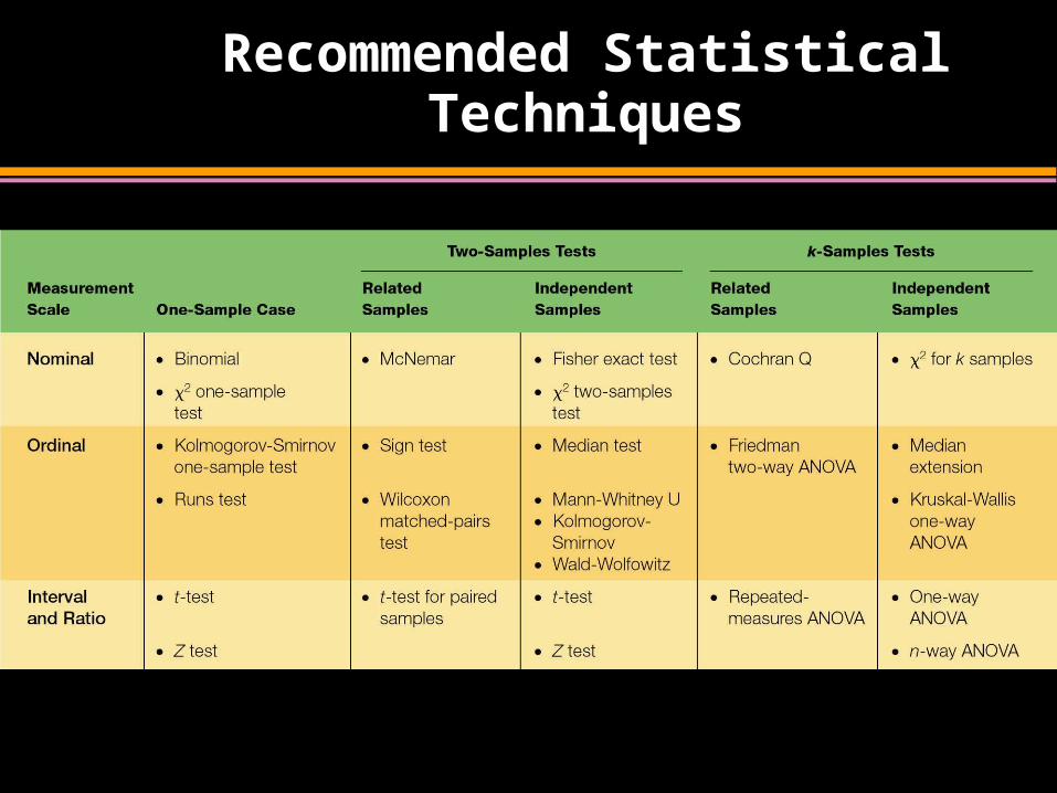
Recommended Statistical Techniques

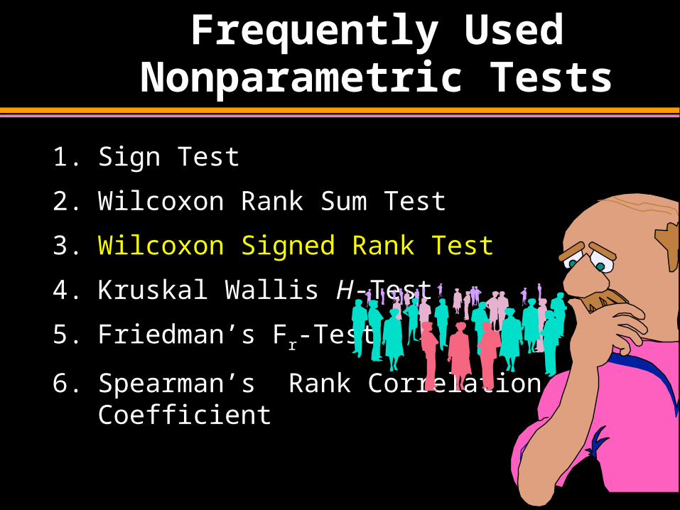
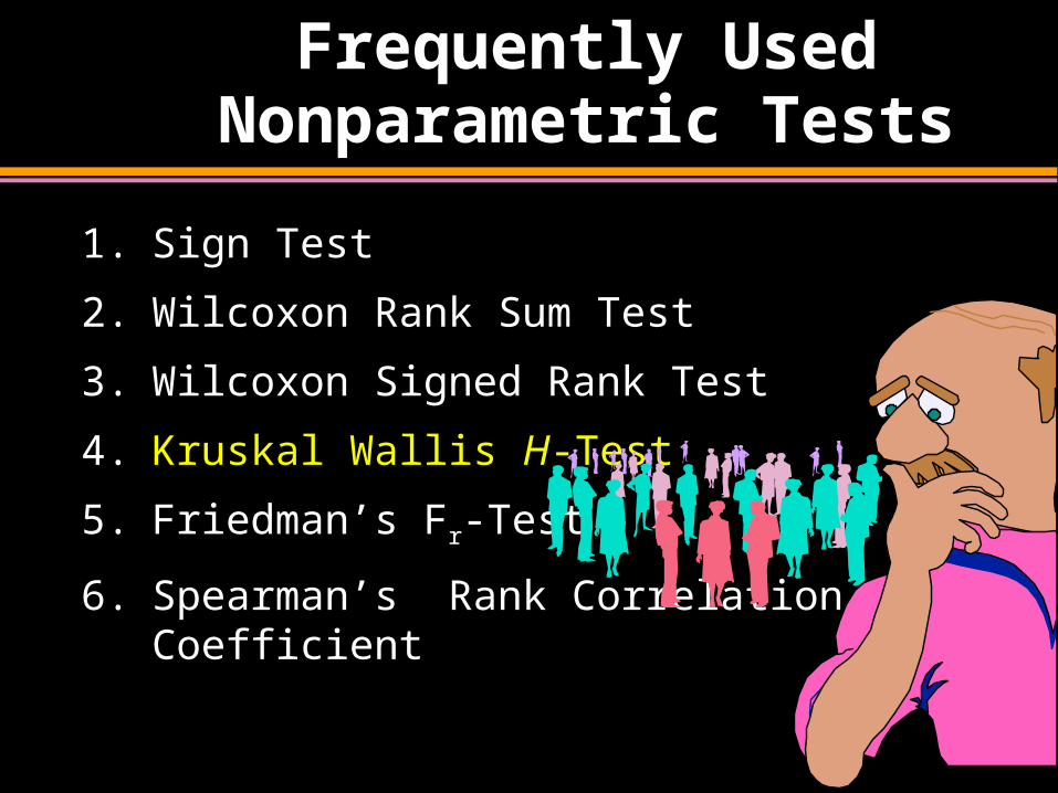
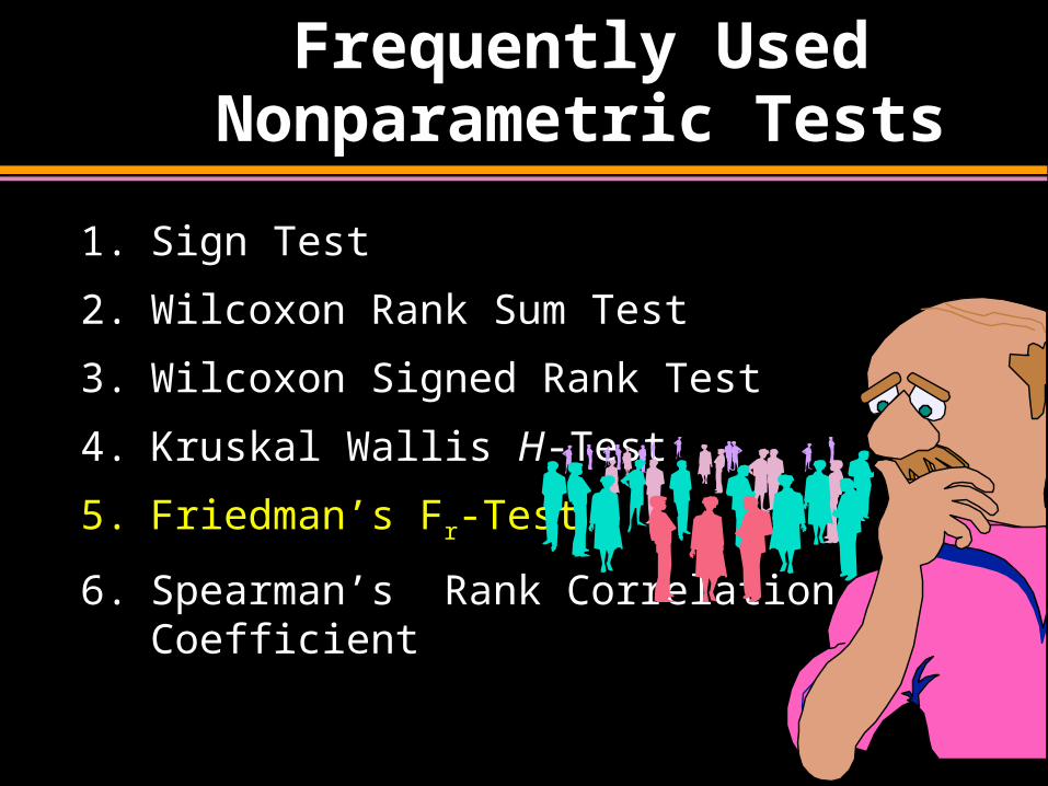
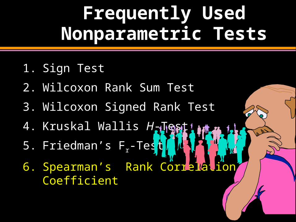
Frequently Used Nonparametric Tests
1. Sign Test
2. Wilcoxon Rank Sum Test
3. Wilcoxon Signed Rank Test
4. Kruskal Wallis H-Test
5. Friedman’s Fr-Test
6. Spearman’s Rank Correlation Coefficient

Single-Variable Chi-Square Test
Single-Variable Chi-Square Test
1. Compares the observed frequencies of categories to frequencies that would be expected if the null hypothesis were true.
2. Data are assumed to be a random sample.
3. Each subject can only have one entry in the chi-square table.
4. The expected frequency for each category should be at least 5.
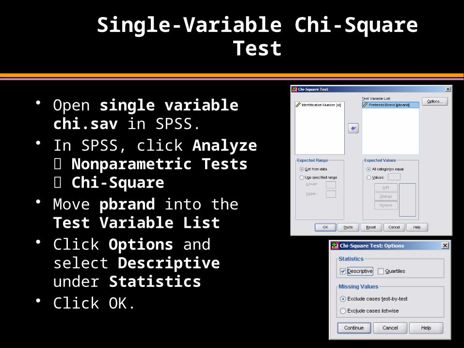
Single-Variable Chi-Square Test
• Open single variable chi.sav in SPSS.
• In SPSS, click Analyze Nonparametric Tests Chi-Square
• Move pbrand into the Test Variable List
• Click Options and select Descriptive under Statistics
• Click OK.
Single-Variable Chi-Square Test
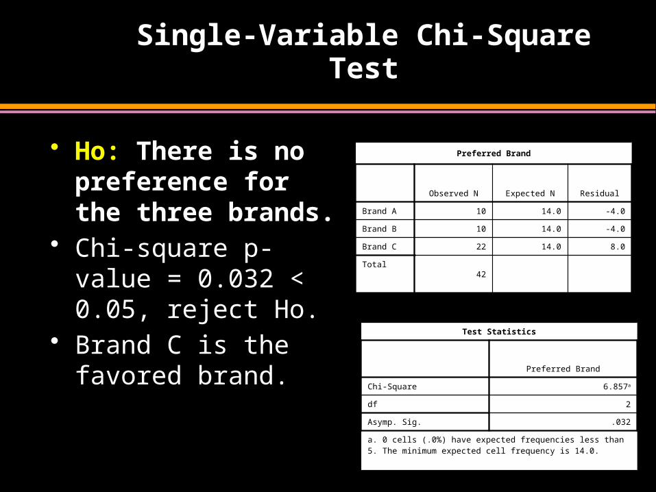
• Ho: There is no preference for the three brands.
• Chi-square p-value = 0.032 < 0.05, reject Ho.
• Brand C is the favored brand.
Test Statistics
Preferred Brand
Chi-Square 6.857a
df 2
Asymp. Sig. .032
a. 0 cells (.0%) have expected frequencies less than 5. The minimum expected cell frequency is 14.0.
Preferred Brand
Observed N Expected N Residual
Brand A 10 14.0 -4.0
Brand B 10 14.0 -4.0
Brand C 22 14.0 8.0
Total42
Sign Test
Sign Test
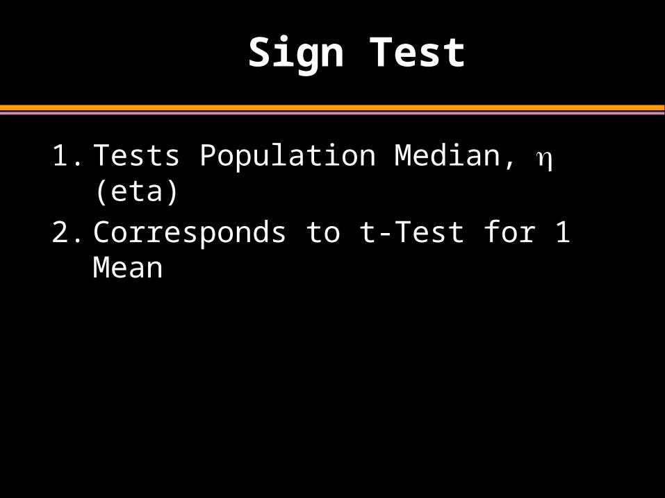
1. Tests Population Median, (eta)
2. Corresponds to t-Test for 1 Mean
Sign Test Uses P-Value
to Make Decision
.031.109
.219.273
.219
.109.031.004 .004
0%
10%
20%
30%
0 1 2 3 4 5 6 7 8 X
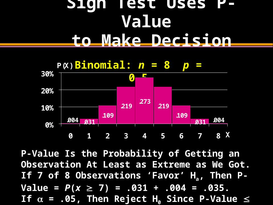
P(X) Binomial: n = 8 p = 0.5
P-Value Is the Probability of Getting an Observation At Least as Extreme as We Got. If 7 of 8 Observations ‘Favor’ Ha, Then P-Value = P(x 7) = .031 + .004 = .035. If = .05, Then Reject H0 Since P-Value .
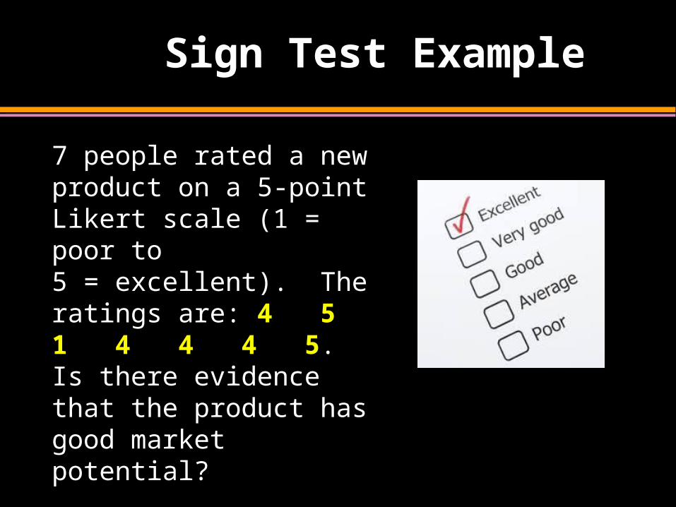
Sign Test Example
7 people rated a new product on a 5-point Likert scale (1 = poor to 5 = excellent). The ratings are: 4 5 1 4 4 4 5. Is there evidence that the product has good market potential?
R Sign Test
If there is no difference in preferences, then we would expect a rating > 3 to be equally likely as a rating < 3.
Hence, the probability that a rating > 3 (and < 3) is binomially distributed with p = 0.5 and n = 7.
Test statistic = 6
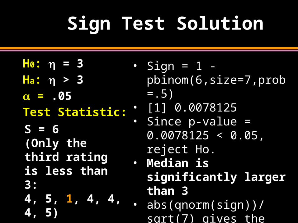
Sign Test Solution
H0: = 3
Ha: > 3
= .05
Test Statistic:
• Sign = 1 -pbinom(6,size=7,prob=.5)
• [1] 0.0078125 • Since p-value = 0.0078125
< 0.05, reject Ho.• Median is significantly
larger than 3• abs(qnorm(sign))/sqrt(7)
gives the approximate effect size.
S = 6 (Only the third rating is less than 3:4, 5, 1, 4, 4, 4, 5)
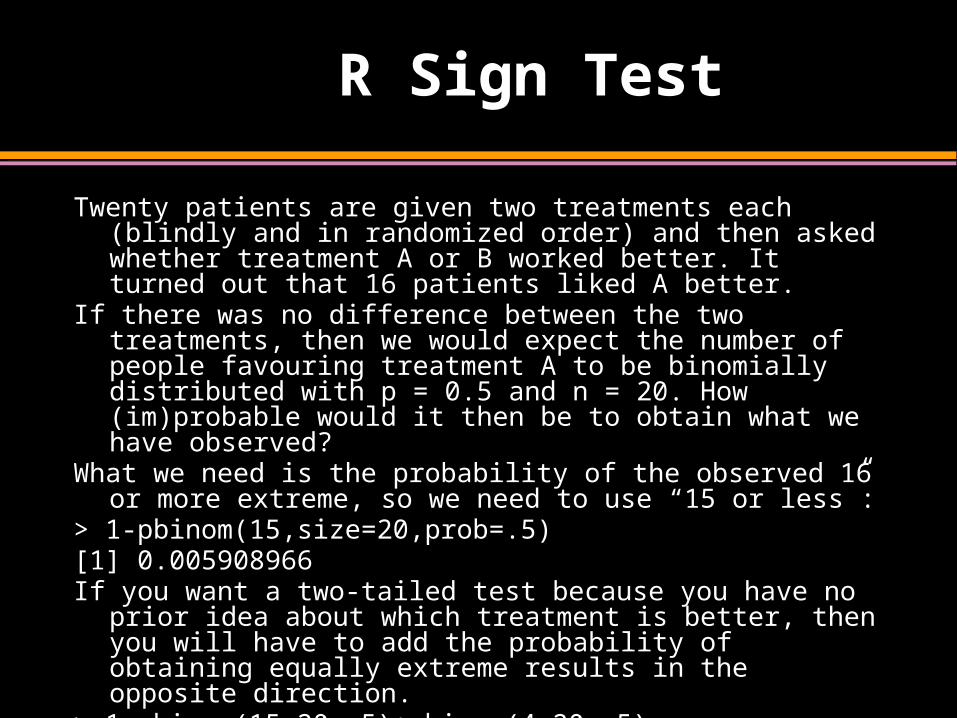
R Sign Test
Twenty patients are given two treatments each (blindly and in randomized order) and then asked whether treatment A or B worked better. It turned out that 16 patients liked A better.
If there was no difference between the two treatments, then we would expect the number of people favouring treatment A to be binomially distributed with p = 0.5 and n = 20. How (im)probable would it then be to obtain what we have observed?
What we need is the probability of the observed 16 or more extreme, so we need to use “15 or less”:
> 1-pbinom(15,size=20,prob=.5)[1] 0.005908966If you want a two-tailed test because you have no prior idea about
which treatment is better, then you will have to add the probability of obtaining equally extreme results in the opposite direction.
> 1-pbinom(15,20,.5)+pbinom(4,20,.5)[1] 0.01181793
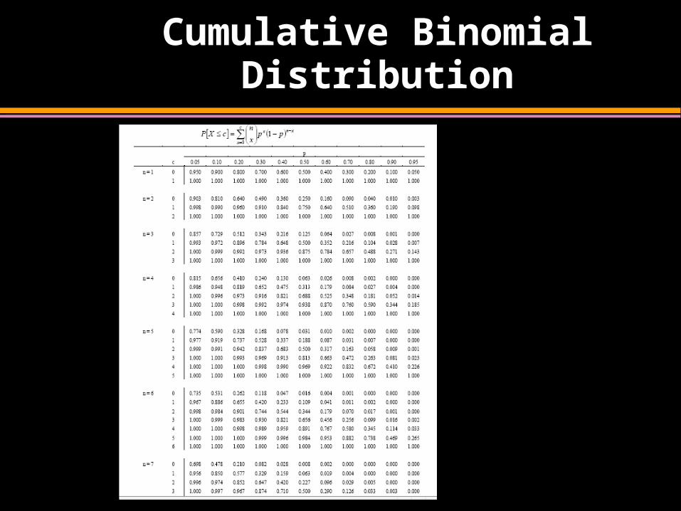
Cumulative Binomial Distribution
SPSS Sign Test
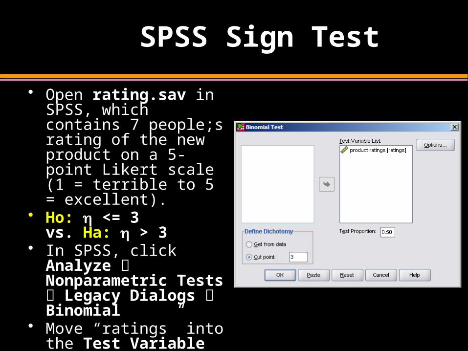
• Open rating.sav in SPSS, which contains 7 people;s rating of the new product on a 5-point Likert scale (1 = terrible to 5 = excellent).
• Ho: <= 3 vs. Ha: > 3
• In SPSS, click Analyze Nonparametric Tests Legacy Dialogs Binomial
• Move “ratings” into the Test Variable List, and set Cut point = 3.
• Click OK.
SPSS Sign Test
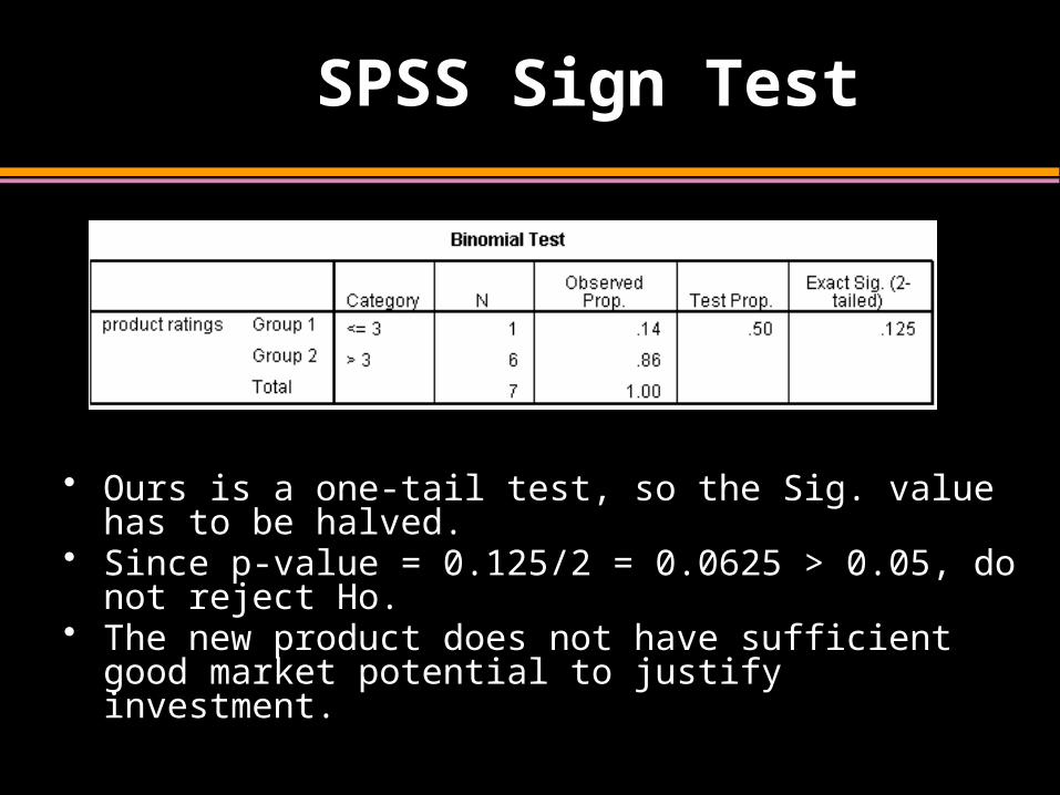
• Ours is a one-tail test, so the Sig. value has to be halved. • Since p-value = 0.125/2 = 0.0625 > 0.05, do not reject Ho.• The new product does not have sufficient good market
potential to justify investment.

Mann-Whitney Test

Frequently Used Nonparametric Tests
1. Sign Test
2. Wilcoxon Rank Sum Test
3. Wilcoxon Signed Rank Test
4. Kruskal Wallis H-Test
5. Friedman’s Fr-Test
6. Spearman’s Rank Correlation Coefficient
Mann-Whitney Test
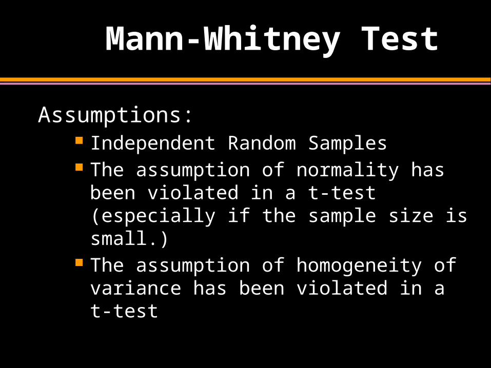
Assumptions: Independent Random Samples The assumption of normality has been
violated in a t-test (especially if the sample size is small.)
The assumption of homogeneity of variance has been violated in a t-test
Mann-Whitney Test
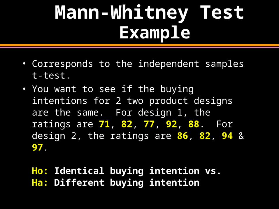
Example• Corresponds to the independent samples t-test.
• You want to see if the buying intentions for 2 two product designs are the same. For design 1, the ratings are 71, 82, 77, 92, 88. For design 2, the ratings are 86, 82, 94 & 97.
Ho: Identical buying intention vs. Ha: Different buying intention
Mann-Whitney Test Computation Table
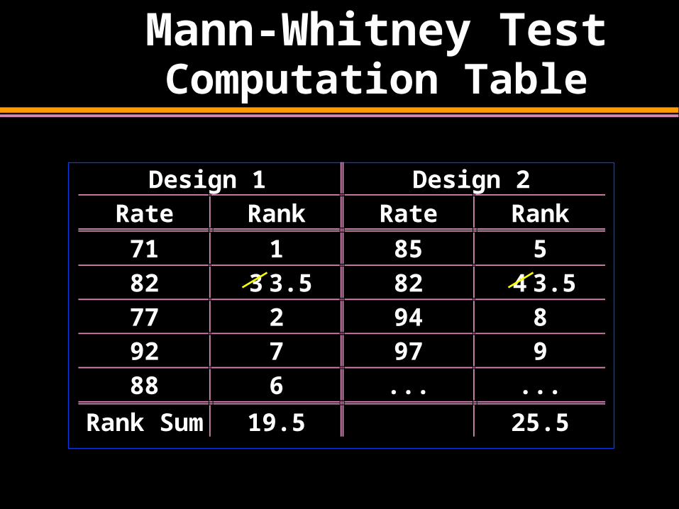
Design 1 Design 2Rate Rank Rate Rank
71 1 85 582 3 3.5 82 4 3.577 2 94 892 7 97 988 6 ... ...
Rank Sum 19.5 25.5
Mann-Whitney Test
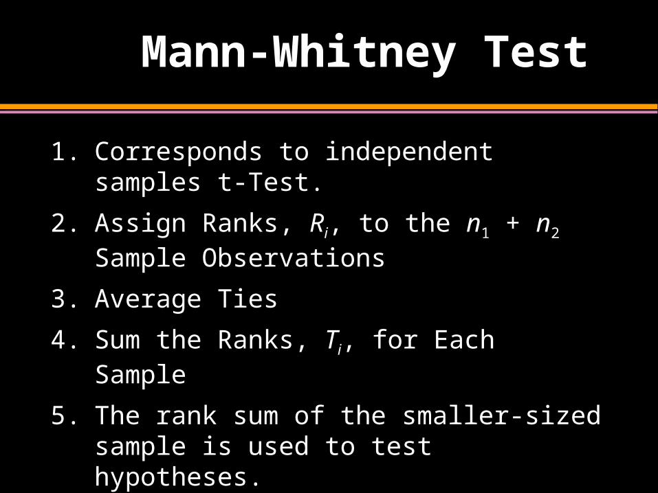
1. Corresponds to independent samples t-Test.
2. Assign Ranks, Ri, to the n1 + n2 Sample Observations
3. Average Ties
4. Sum the Ranks, Ti, for Each Sample
5. The rank sum of the smaller-sized sample is used to test hypotheses.
Mann-Whitney Test
Table (Portion)
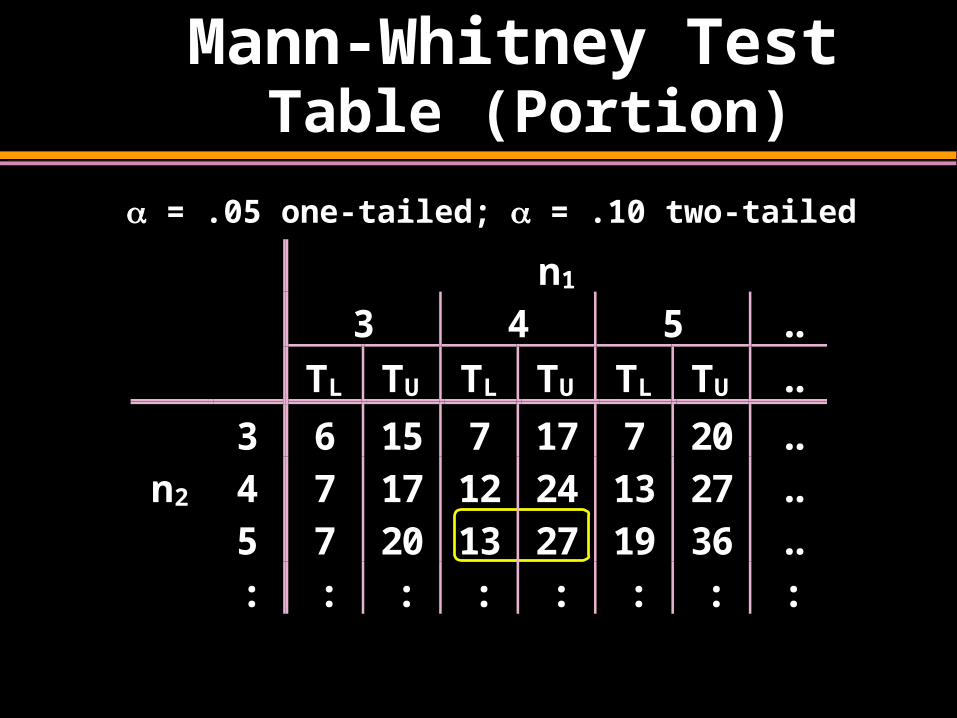
n1
3 4 5 ..
TL TU TL TU TL TU ..
3 6 15 7 17 7 20 ..n2 4 7 17 12 24 13 27 ..
5 7 20 13 27 19 36 ..: : : : : : : :
= .05 one-tailed; = .10 two-tailed
Mann-Whitney Test
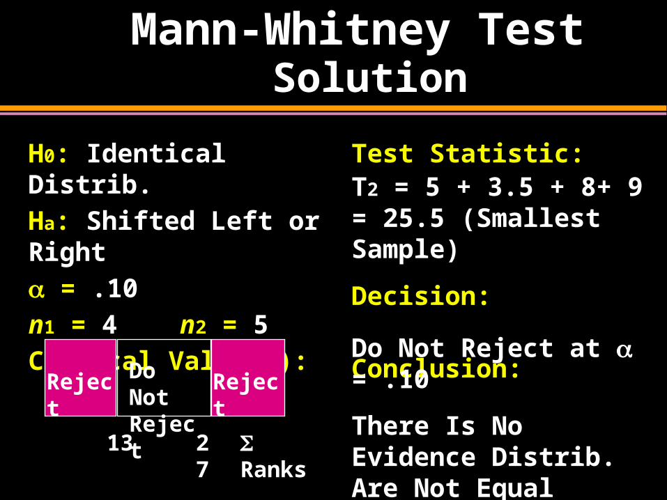
SolutionH0: Identical Distrib.
Ha: Shifted Left or Right
= .10
n1 = 4 n2 = 5
Critical Value(s):
Test Statistic:
Decision:
Conclusion:Do Not Reject at = .10
There Is No Evidence Distrib. Are Not Equal
Reject RejectDo Not Reject
13 27 Ranks
T2 = 5 + 3.5 + 8+ 9 = 25.5 (Smallest Sample)
R Wilcoxon Rank Sum Test
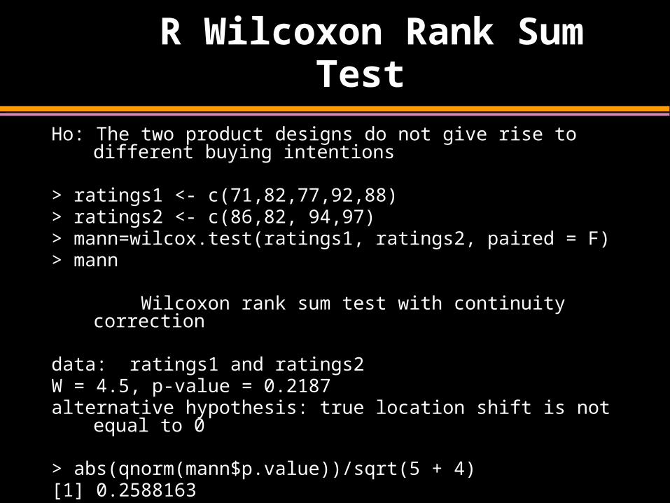
Ho: The two product designs do not give rise to different buying intentions
> ratings1 <- c(71,82,77,92,88)> ratings2 <- c(86,82, 94,97)> mann=wilcox.test(ratings1, ratings2, paired = F)> mann
Wilcoxon rank sum test with continuity correction
data: ratings1 and ratings2W = 4.5, p-value = 0.2187alternative hypothesis: true location shift is not equal to 0
> abs(qnorm(mann$p.value))/sqrt(5 + 4)[1] 0.2588163>
SPSS Mann-Whitney Test
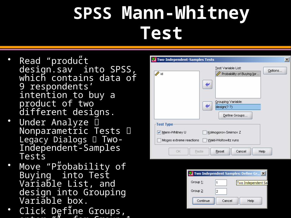
• Read “product design.sav” into SPSS, which contains data of 9 respondents’ intention to buy a product of two different designs.
• Under Analyze Nonparametric Tests Legacy Dialogs Two-Independent-Samples Tests
• Move “Probability of Buying” into Test Variable List, and design into Grouping Variable box.
• Click Define Groups, enter “1” for Group 1, and “2” for Group 2.
• Click Continue and then OK to get your output.
SPSS Mann-Whitney Test
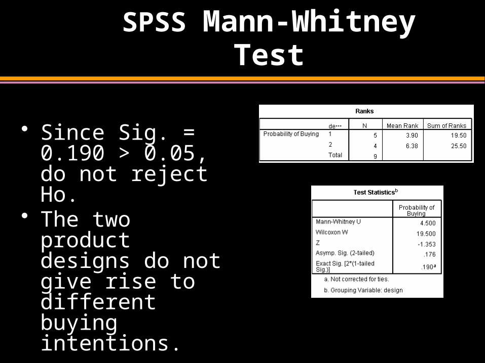
• Since Sig. = 0.190 > 0.05, do not reject Ho.
• The two product designs do not give rise to different buying intentions.

Wilcoxon Signed Rank Test
Frequently Used Nonparametric Tests
1. Sign Test
2. Wilcoxon Rank Sum Test
3. Wilcoxon Signed Rank Test
4. Kruskal Wallis H-Test
5. Friedman’s Fr-Test
6. Spearman’s Rank Correlation Coefficient
Wilcoxon Signed Rank Test
1. For repeated measurements taken from the same subject.
2. Corresponds to paired samples t-test.
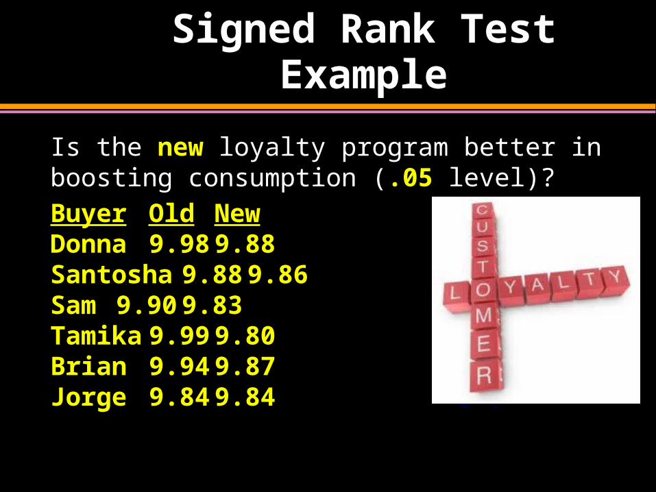
Signed Rank TestExample
Is the new loyalty program better in boosting consumption (.05 level)?
Buyer Old NewDonna 9.98 9.88Santosha 9.88 9.86Sam 9.90 9.83Tamika 9.99 9.80Brian9.94 9.87Jorge 9.84 9.84
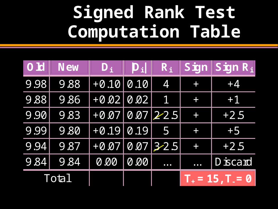
Signed Rank Test Computation Table
Old New Di |Di| Ri Sign Sign Ri
9.98 9.88 +0.10 0.10 4 + +4
9.88 9.86 +0.02 0.02 1 + +1
9.90 9.83 +0.07 0.07 2 2.5 + +2.5
9.99 9.80 +0.19 0.19 5 + +5
9.94 9.87 +0.07 0.07 3 2.5 + +2.5
9.84 9.84 0.00 0.00 ... ... Discard
Total T+ = 15, T- = 0
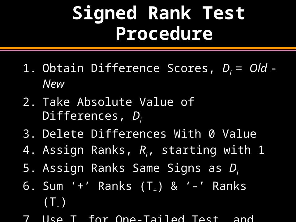
Signed Rank Test Procedure
1. Obtain Difference Scores, Di = Old - New
2. Take Absolute Value of Differences, Di
3. Delete Differences With 0 Value
4. Assign Ranks, Ri, starting with 1
5. Assign Ranks Same Signs as Di
6. Sum ‘+’ Ranks (T+) & ‘-’ Ranks (T-)
7. Use T- for One-Tailed Test, and the Smaller of T- or T+ for 2-Tail Test
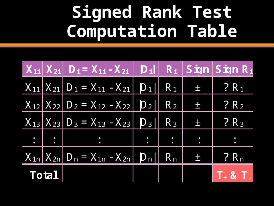
Signed Rank Test Computation Table
X1i X2i Di = X1i - X2i |Di| Ri Sign Sign Ri
X11 X21 D1 = X11 - X21 |D1| R1 ± ? R1
X12 X22 D2 = X12 - X22 |D2| R2 ± ? R2
X13 X23 D3 = X13 - X23 |D3| R3 ± ? R3
: : : : : : :
X1n X2n Dn = X1n - X2n |Dn| Rn ± ? Rn
Total T+ & T-
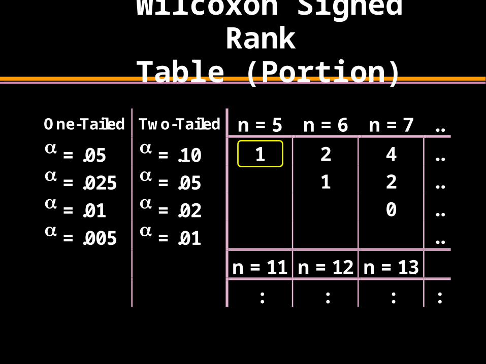
Wilcoxon Signed Rank
Table (Portion)
One-Tailed Two-Tailed n = 5 n = 6 n = 7 .. = .05 = .10 1 2 4 .. = .025 = .05 1 2 .. = .01 = .02 0 .. = .005 = .01 ..
n = 11 n = 12 n = 13
: : : :
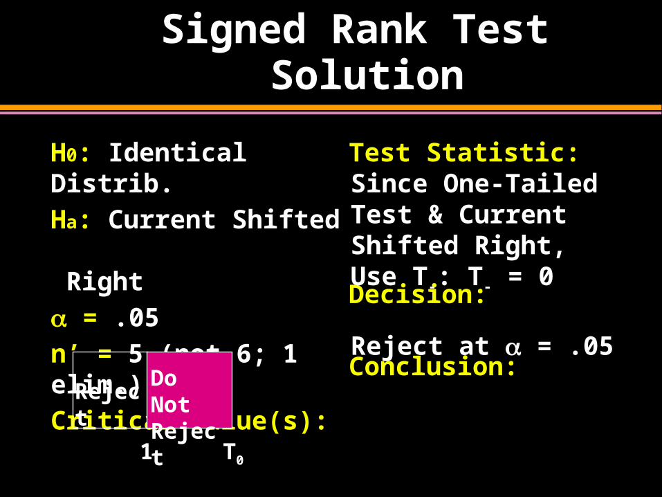
Signed Rank Test Solution
H0: Identical Distrib.
Ha: Current Shifted Right
= .05
n’ = 5 (not 6; 1 elim.)
Critical Value(s):
Test Statistic:
Decision:
Conclusion:Reject at = .05
RejectDo Not Reject
1 T0
Since One-Tailed Test & Current Shifted Right, Use T-: T- = 0
R Signed Rank Test
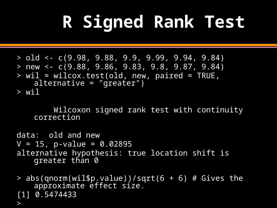
> old <- c(9.98, 9.88, 9.9, 9.99, 9.94, 9.84)> new <- c(9.88, 9.86, 9.83, 9.8, 9.87, 9.84)> wil = wilcox.test(old, new, paired = TRUE, alternative = "greater")> wil
Wilcoxon signed rank test with continuity correction
data: old and newV = 15, p-value = 0.02895alternative hypothesis: true location shift is greater than 0
> abs(qnorm(wil$p.value))/sqrt(6 + 6) # Gives the approximate effect size.
[1] 0.5474433>
SPSS Signed Rank Test
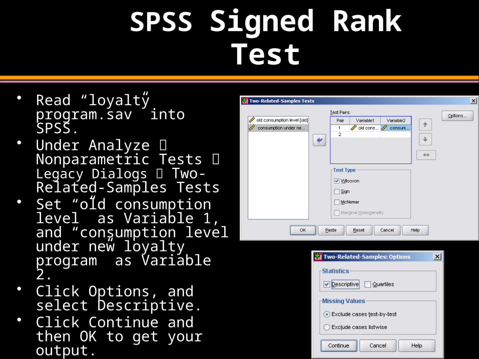
• Read “loyalty program.sav” into SPSS.
• Under Analyze Nonparametric Tests Legacy Dialogs Two-Related-Samples Tests
• Set “old consumption level” as Variable 1, and “consumption level under new loyalty program” as Variable 2.
• Click Options, and select Descriptive.
• Click Continue and then OK to get your output.
SPSS Signed Rank Test
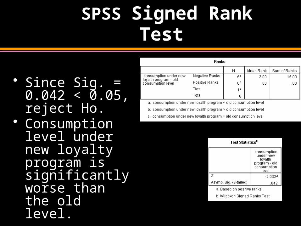
• Since Sig. = 0.042 < 0.05, reject Ho.
• Consumption level under new loyalty program is significantly worse than the old level.
Wilcoxon test
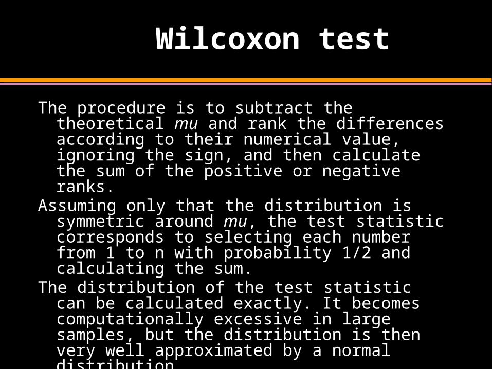
The procedure is to subtract the theoretical mu and rank the differences according to their numerical value, ignoring the sign, and then calculate the sum of the positive or negative ranks.
Assuming only that the distribution is symmetric around mu, the test statistic corresponds to selecting each number from 1 to n with probability 1/2 and calculating the sum.
The distribution of the test statistic can be calculated exactly. It becomes computationally excessive in large samples, but the distribution is then very well approximated by a normal distribution.
> wilcox.test(daily.intake, mu=7725)The test statistic V is the sum of the positive ranks.

Kruskal-Wallis H-Test
Frequently Used Nonparametric Tests
1. Sign Test
2. Wilcoxon Rank Sum Test
3. Wilcoxon Signed Rank Test
4. Kruskal Wallis H-Test
5. Friedman’s Fr-Test
6. Spearman’s Rank Correlation Coefficient
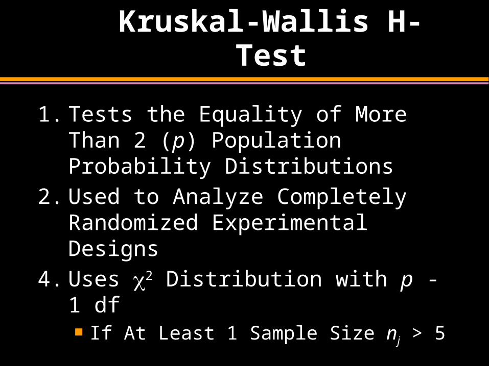
Kruskal-Wallis H-Test
1. Tests the Equality of More Than 2 (p) Population Probability Distributions
2. Used to Analyze Completely Randomized Experimental Designs
4. Uses 2 Distribution with p - 1 df If At Least 1 Sample Size nj > 5
Kruskal-Wallis H-Test Assumptions
1. Corresponds to ANOVA for More Than 2 Populations
2. Independent, Random Samples
3. At Least 5 Observations Per Sample
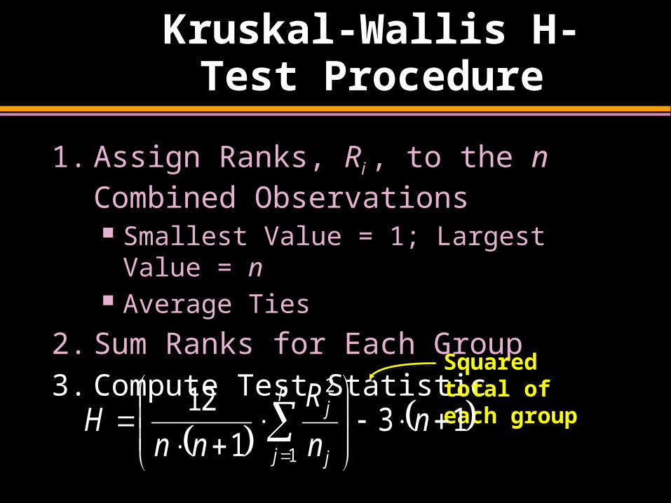
Kruskal-Wallis H-Test Procedure
1. Assign Ranks, Ri , to the n Combined Observations Smallest Value = 1; Largest Value = n Average Ties
2. Sum Ranks for Each Group
3. Compute Test Statistic
131
12
1
2
nn
R
nnH
p
j j
j
Squared total of each group
Kruskal-Wallis H-Test Example
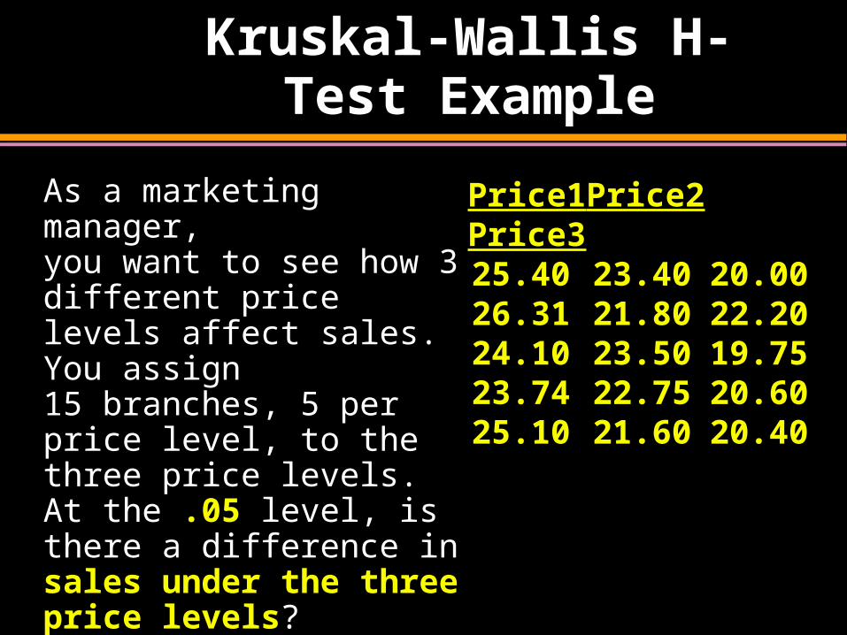
As a marketing manager, you want to see how 3 different price levels affect sales. You assign 15 branches, 5 per price level, to the three price levels. At the .05 level, is there a difference in sales under the three price levels?
Price1 Price2 Price325.40 23.40 20.0026.31 21.80 22.2024.10 23.50 19.7523.74 22.75 20.6025.10 21.60 20.40
Kruskal-Wallis H-Test
Solution
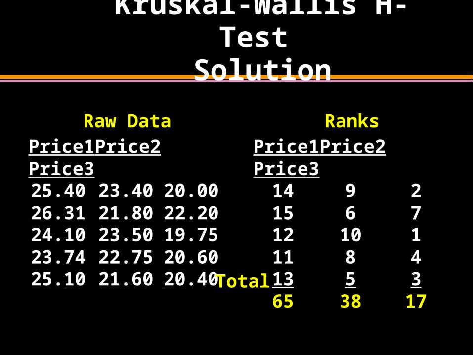
Raw Data
Price1 Price2 Price325.40 23.40 20.0026.31 21.80 22.2024.10 23.50 19.7523.74 22.75 20.6025.10 21.60 20.40
Ranks
Price1 Price2 Price314 9 215 6 712 10 111 8 413 5 365 38 17Total
Kruskal-Wallis H-Test
Solution
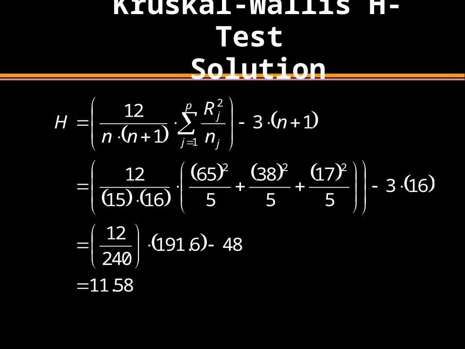
58.11
486.191240
12
1635
17
5
38
5
65
1615
12
131
12
222
1
2
nn
R
nnH
p
j j
j
20 5.991
Kruskal-Wallis H-Test
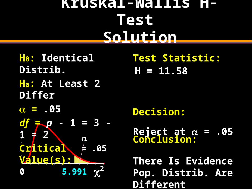
SolutionH0: Identical Distrib.
Ha: At Least 2 Differ
= .05
df = p - 1 = 3 - 1 = 2
Critical Value(s):
Test Statistic:
Decision:
Conclusion:Reject at = .05
There Is Evidence Pop. Distrib. Are Different
= .05
H = 11.58
Kruskal-Wallis H-Test
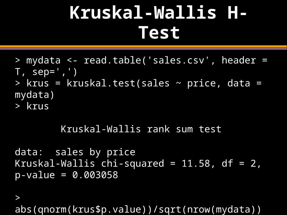
> mydata <- read.table('sales.csv', header = T, sep=',')> krus = kruskal.test(sales ~ price, data = mydata)> krus
Kruskal-Wallis rank sum test
data: sales by priceKruskal-Wallis chi-squared = 11.58, df = 2, p-value = 0.003058
> abs(qnorm(krus$p.value))/sqrt(nrow(mydata)) # Gives the approximate effect size.[1] 0.7078519>
Multiple Comparison
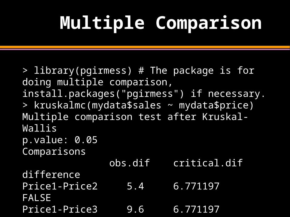
> library(pgirmess) # The package is for doing multiple comparison, install.packages("pgirmess") if necessary.> kruskalmc(mydata$sales ~ mydata$price)Multiple comparison test after Kruskal-Wallis p.value: 0.05 Comparisons obs.dif critical.dif differencePrice1-Price2 5.4 6.771197 FALSEPrice1-Price3 9.6 6.771197 TRUEPrice2-Price3 4.2 6.771197 FALSE

SPSS Kruskal-Wallis H-Test
• Read “sales.sav” into SPSS.
• Under Analyze Nonparametric Tests Legacy Dialogs K Independent Samples
• Move “sales” under Test Variable List, and “price” in Grouping Variable Box.
• Click Define Range, enter ‘1’ as Minimum and ‘3’ as Maximum.
• Click Options, and select Descriptive.
• Click Continue and then OK to get your output.
SPSS Kruskal-Wallis H-Test
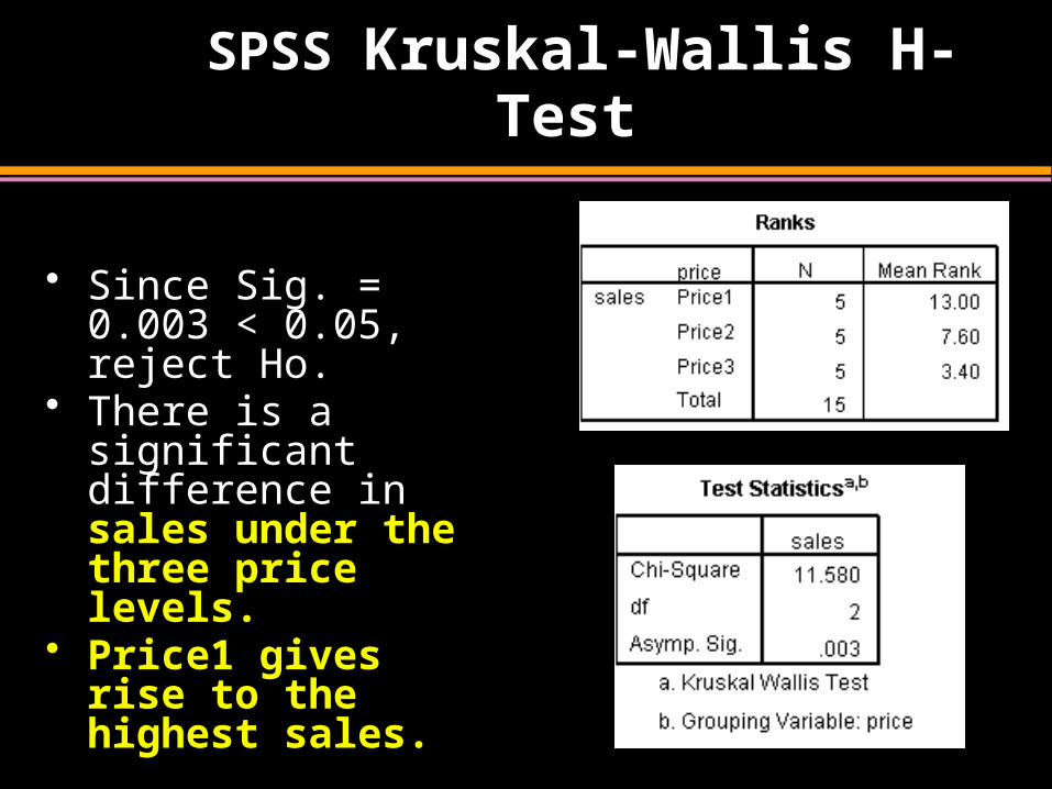
• Since Sig. = 0.003 < 0.05, reject Ho.
• There is a significant difference in sales under the three price levels.
• Price1 gives rise to the highest sales.
Friedman Fr-Test
Frequently Used Nonparametric Tests
1. Sign Test
2. Wilcoxon Rank Sum Test
3. Wilcoxon Signed Rank Test
4. Kruskal Wallis H-Test
5. Friedman’s Fr-Test
6. Spearman’s Rank Correlation Coefficient
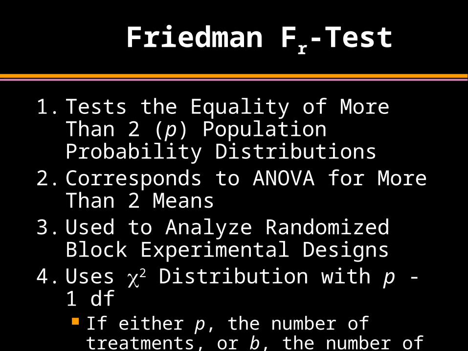
Friedman Fr-Test
1. Tests the Equality of More Than 2 (p) Population Probability Distributions
2. Corresponds to ANOVA for More Than 2 Means
3. Used to Analyze Randomized Block Experimental Designs
4. Uses 2 Distribution with p - 1 df If either p, the number of treatments, or b,
the number of blocks, exceeds 5
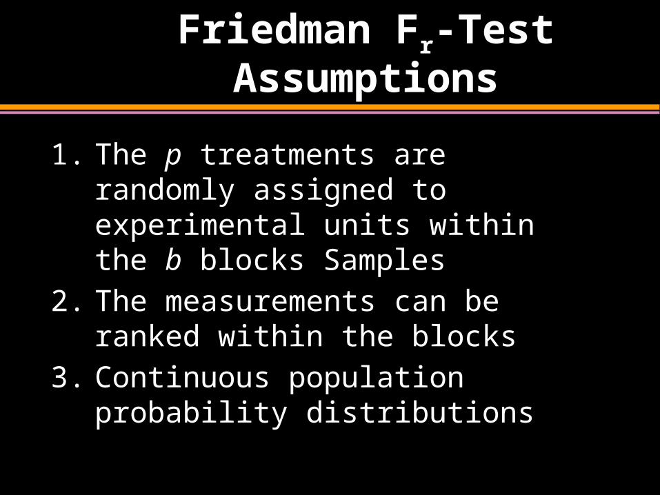
Friedman Fr-Test Assumptions
1. The p treatments are randomly assigned to experimental units within the b blocks Samples
2. The measurements can be ranked within the blocks
3. Continuous population probability distributions
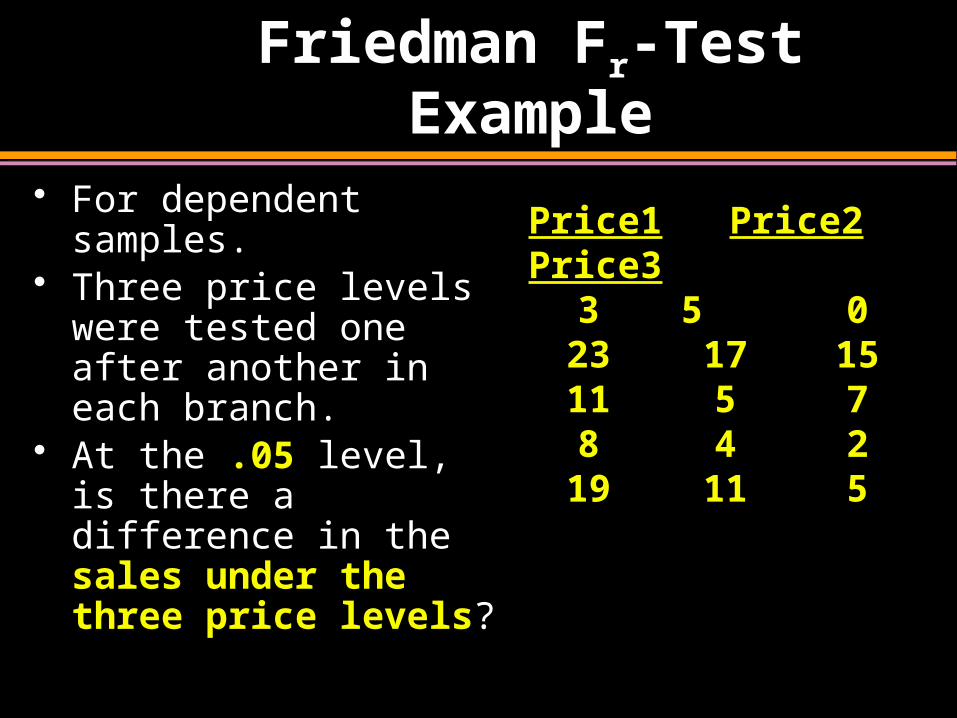
Friedman Fr-Test Example
• For dependent samples.• Three price levels were
tested one after another in each branch.
• At the .05 level, is there a difference in the sales under the three price levels?
Price1 Price2 Price33 5 0
23 17 1511 5 78 4 2
19 11 5
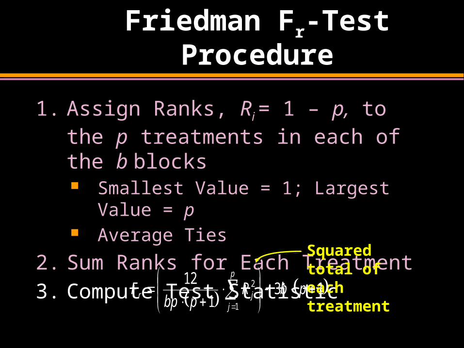
Friedman Fr-Test Procedure
1. Assign Ranks, Ri = 1 – p, to the p treatments in each of the b blocks Smallest Value = 1; Largest Value = p Average Ties
2. Sum Ranks for Each Treatment
3. Compute Test Statistic
131
12
1
2
pbRpbp
Fp
jjr
Squared total of each treatment
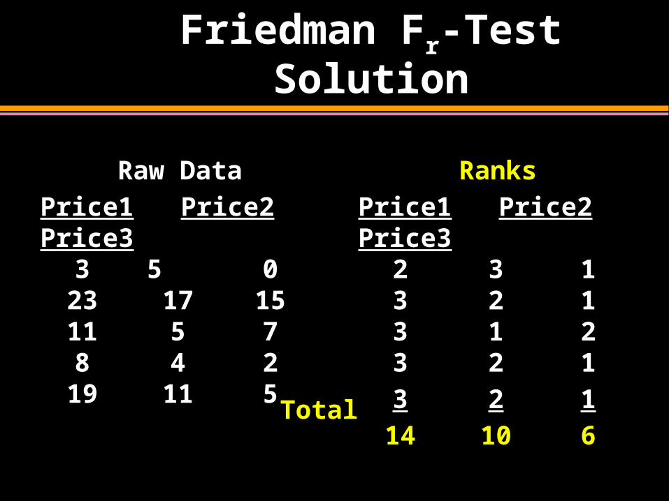
Friedman Fr-Test Solution
Raw Data
Price1 Price2 Price33 5 0
23 17 1511 5 78 4 2
19 11 5
Ranks
Price1 Price2 Price32 3 13 2 13 1 23 2 1
3 2 1
14 10 6Total
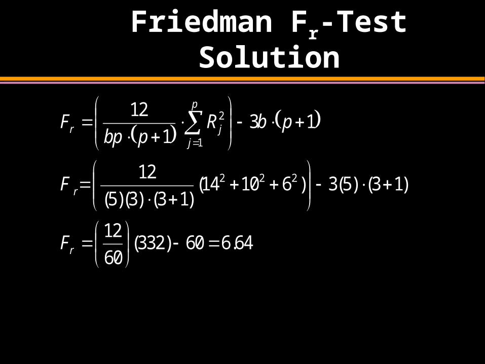
Friedman Fr-Test Solution
64.660)332(60
12
)13()5(3)61014()13()3)(5(
12
131
12
222
1
2
r
r
p
jjr
F
F
pbRpbp
F
20 5.991
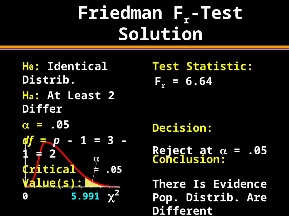
Friedman Fr-Test Solution
H0: Identical Distrib.
Ha: At Least 2 Differ
= .05
df = p - 1 = 3 - 1 = 2
Critical Value(s):
Test Statistic:
Decision:
Conclusion:Reject at = .05
There Is Evidence Pop. Distrib. Are Different
= .05
Fr = 6.64
Friedman Fr-Test
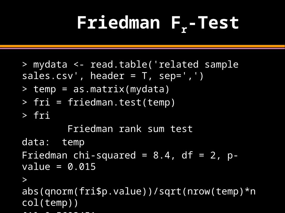
> mydata <- read.table('related sample sales.csv', header = T, sep=',')
> temp = as.matrix(mydata)
> fri = friedman.test(temp)
> fri
Friedman rank sum test
data: temp
Friedman chi-squared = 8.4, df = 2, p-value = 0.015
> abs(qnorm(fri$p.value))/sqrt(nrow(temp)*ncol(temp))
[1] 0.5603451
Friedman Fr-Test
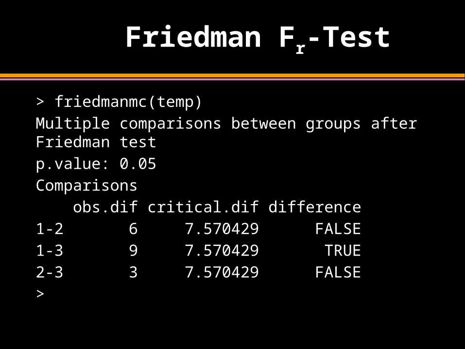
> friedmanmc(temp)
Multiple comparisons between groups after Friedman test
p.value: 0.05
Comparisons
obs.dif critical.dif difference
1-2 6 7.570429 FALSE
1-3 9 7.570429 TRUE
2-3 3 7.570429 FALSE
>
SPSS Friedman Fr-Test
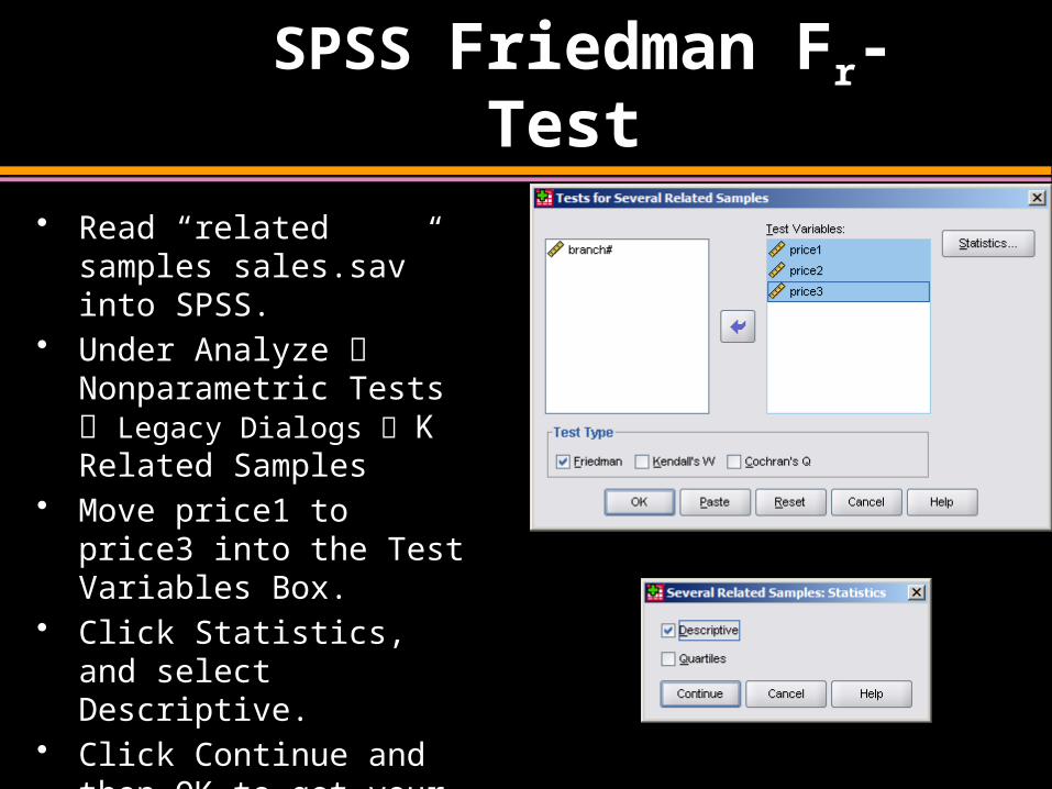
• Read “related samples sales.sav” into SPSS.
• Under Analyze Nonparametric Tests Legacy Dialogs K Related Samples
• Move price1 to price3 into the Test Variables Box.
• Click Statistics, and select Descriptive.
• Click Continue and then OK to get your output.
SPSS Friedman Fr-Test
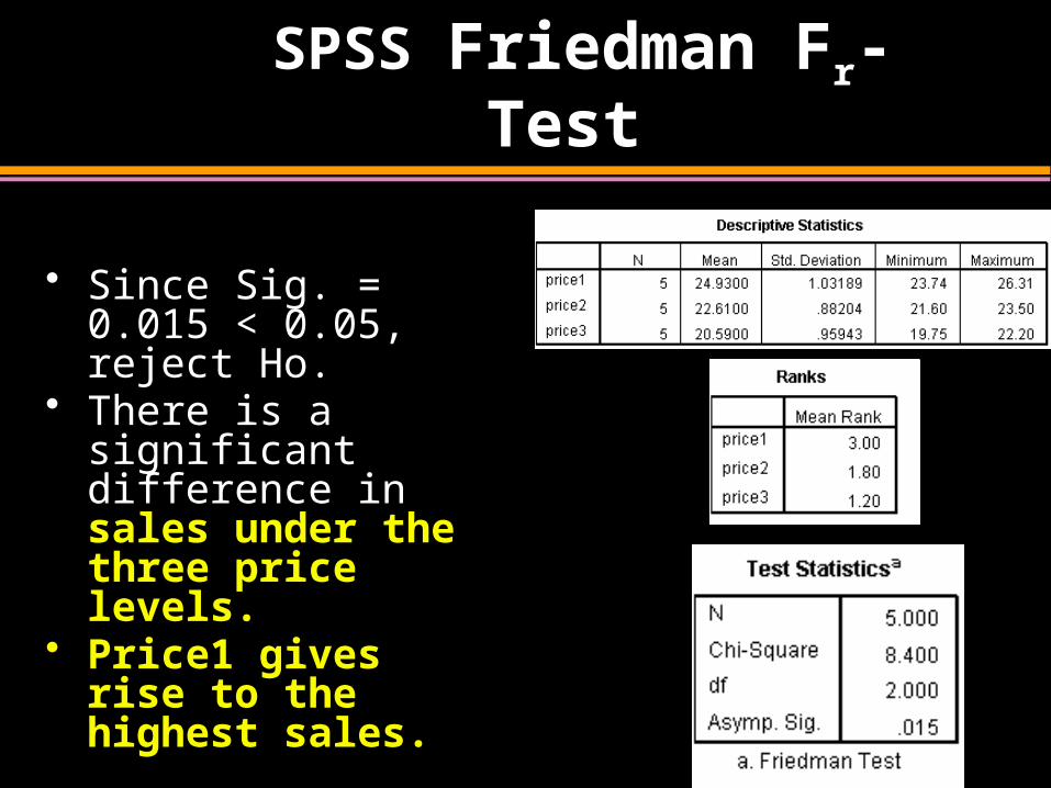
• Since Sig. = 0.015 < 0.05, reject Ho.
• There is a significant difference in sales under the three price levels.
• Price1 gives rise to the highest sales.
Frequently Used Nonparametric Tests
1. Sign Test
2. Wilcoxon Rank Sum Test
3. Wilcoxon Signed Rank Test
4. Kruskal Wallis H-Test
5. Friedman’s Fr-Test
6. Spearman’s Rank Correlation Coefficient
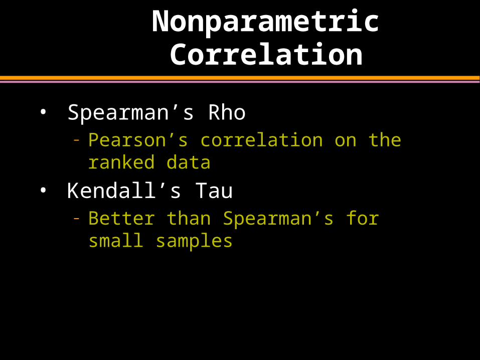
Nonparametric Correlation
• Spearman’s Rho– Pearson’s correlation on the ranked data
• Kendall’s Tau– Better than Spearman’s for small samples
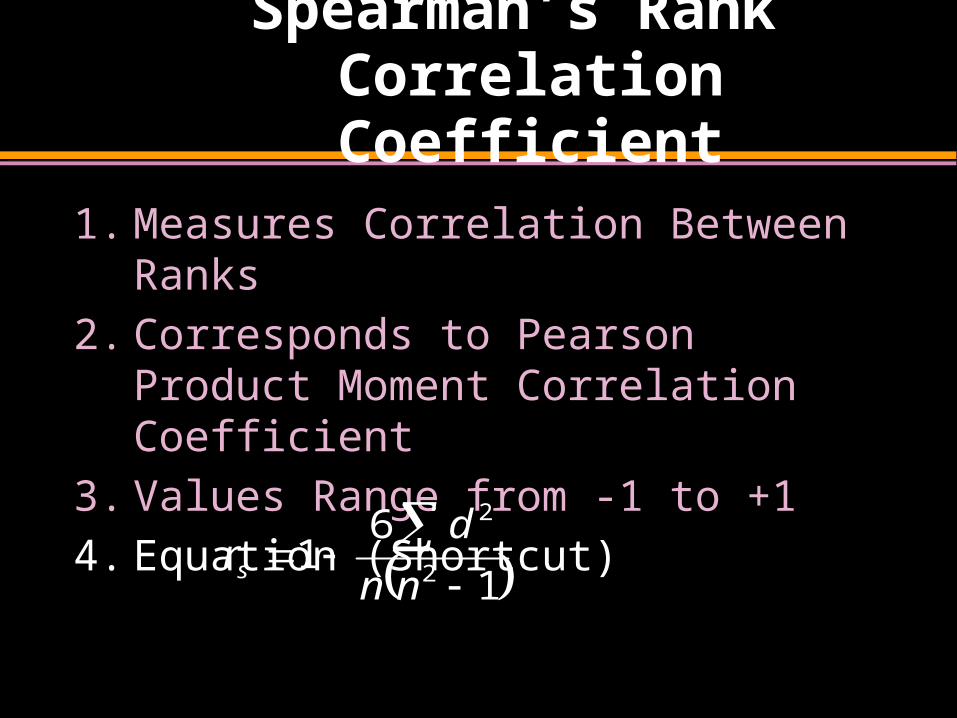
Spearman’s Rank Correlation Coefficient
1. Measures Correlation Between Ranks
2. Corresponds to Pearson Product Moment Correlation Coefficient
3. Values Range from -1 to +1
4. Equation (Shortcut)
1
61
2
2
nn
drs
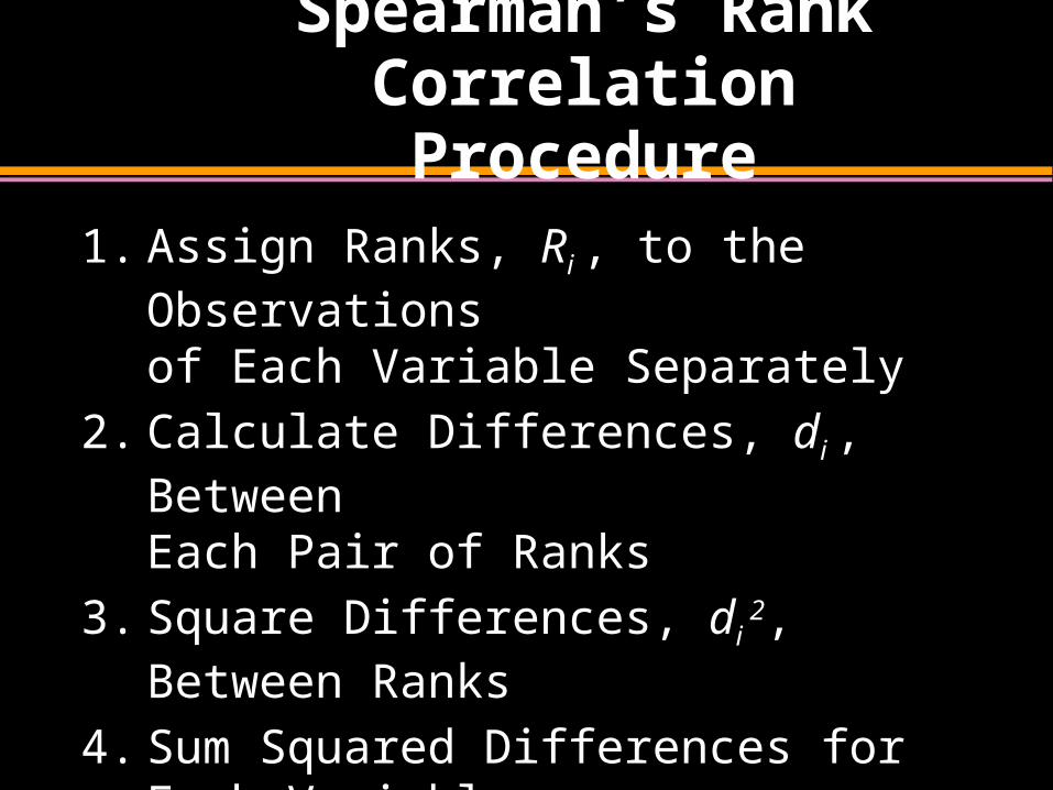
Spearman’s Rank Correlation Procedure
1. Assign Ranks, Ri , to the Observations of Each Variable Separately
2. Calculate Differences, di , Between Each Pair of Ranks
3. Square Differences, di 2, Between Ranks
4. Sum Squared Differences for Each Variable
5. Use Shortcut Approximation Formula
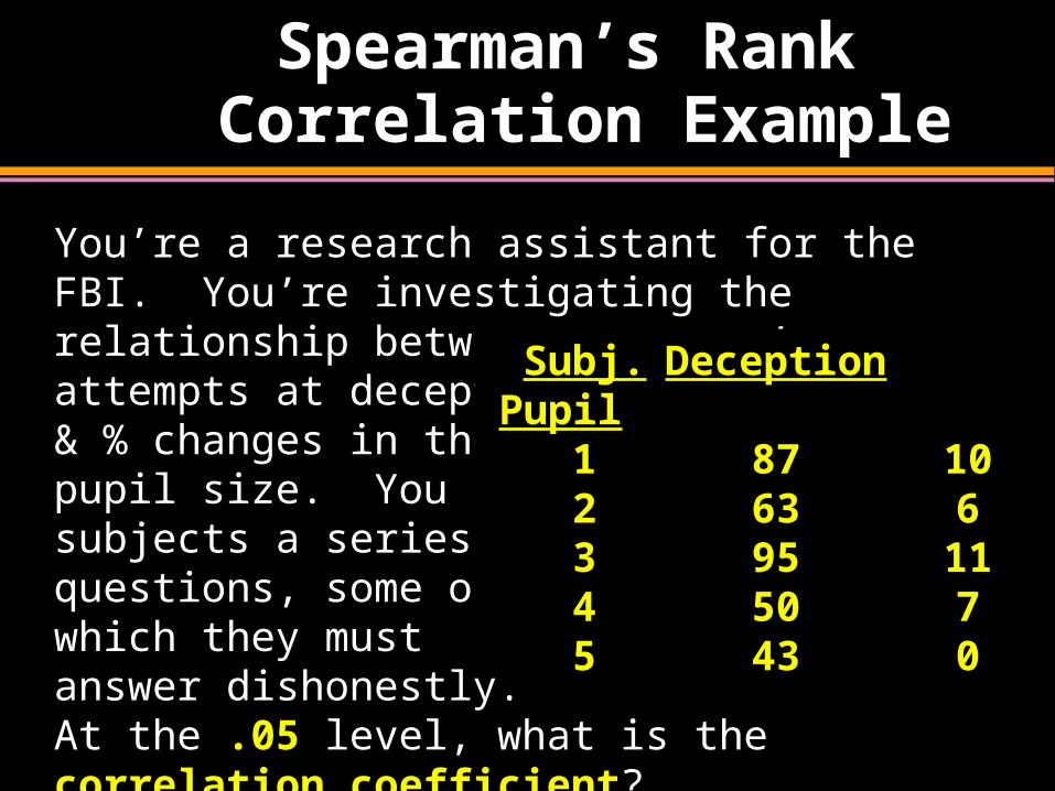
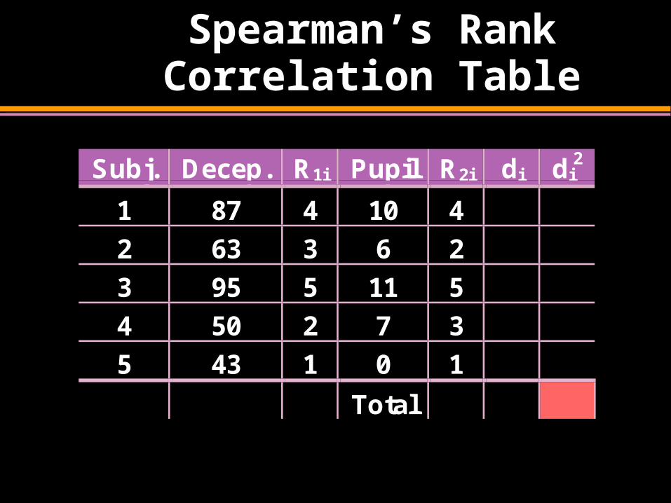
Spearman’s Rank Correlation Example
You’re a research assistant for the FBI. You’re investigating the relationship between a person’s attempts at deception & % changes in their pupil size. You ask subjects a series of questions, some of which they must answer dishonestly. At the .05 level, what is the correlation coefficient?
Subj. DeceptionPupil
1 87 102 63 63 95 114 50 75 43 0
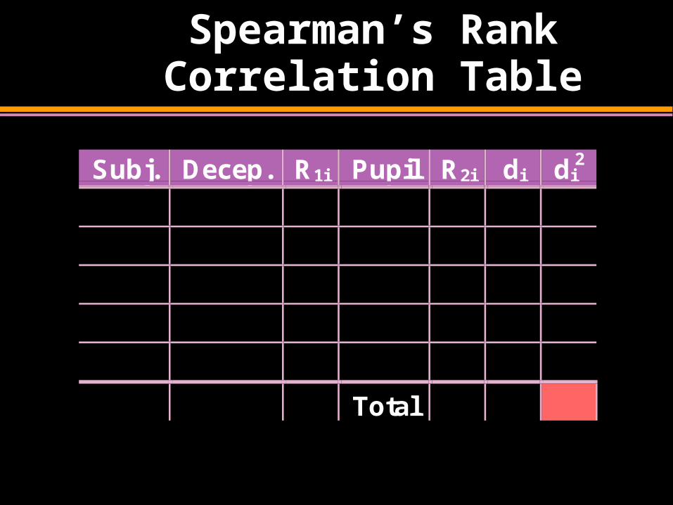
Spearman’s Rank Correlation Table
Subj. Decep. R1i Pupil R2i di di2
Total
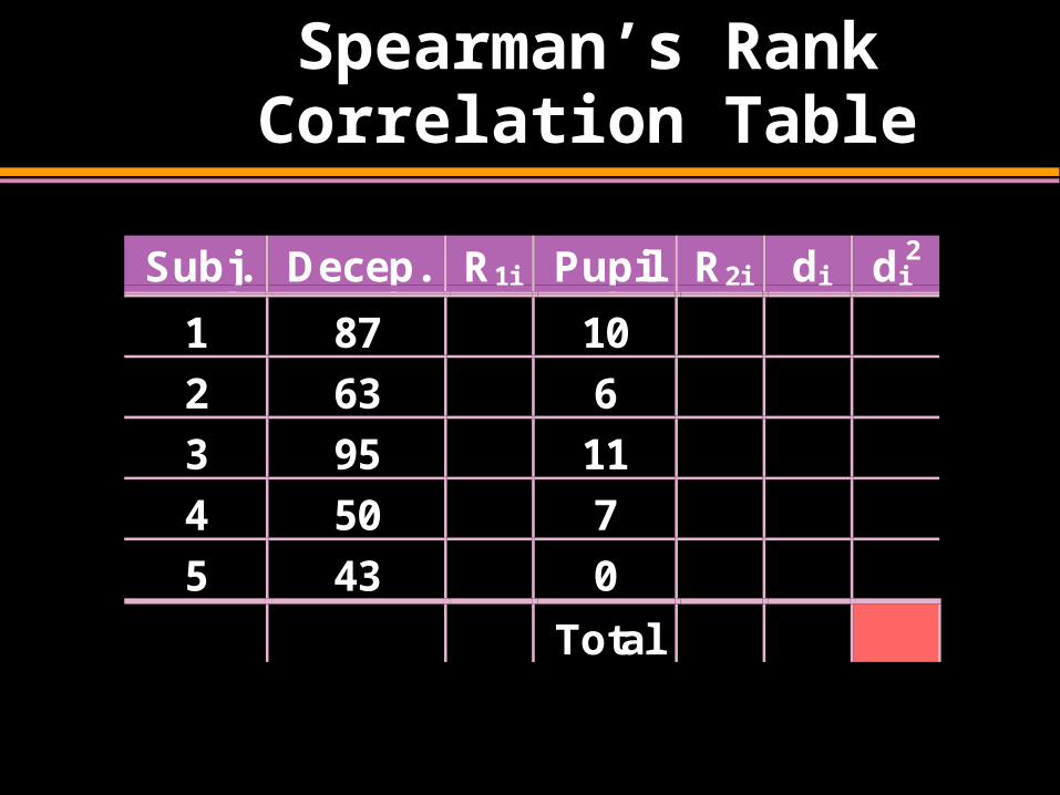
Spearman’s Rank Correlation Table
Subj. Decep. R1i Pupil R2i di di2
1 87 10
2 63 6
3 95 11
4 50 7
5 43 0
Total
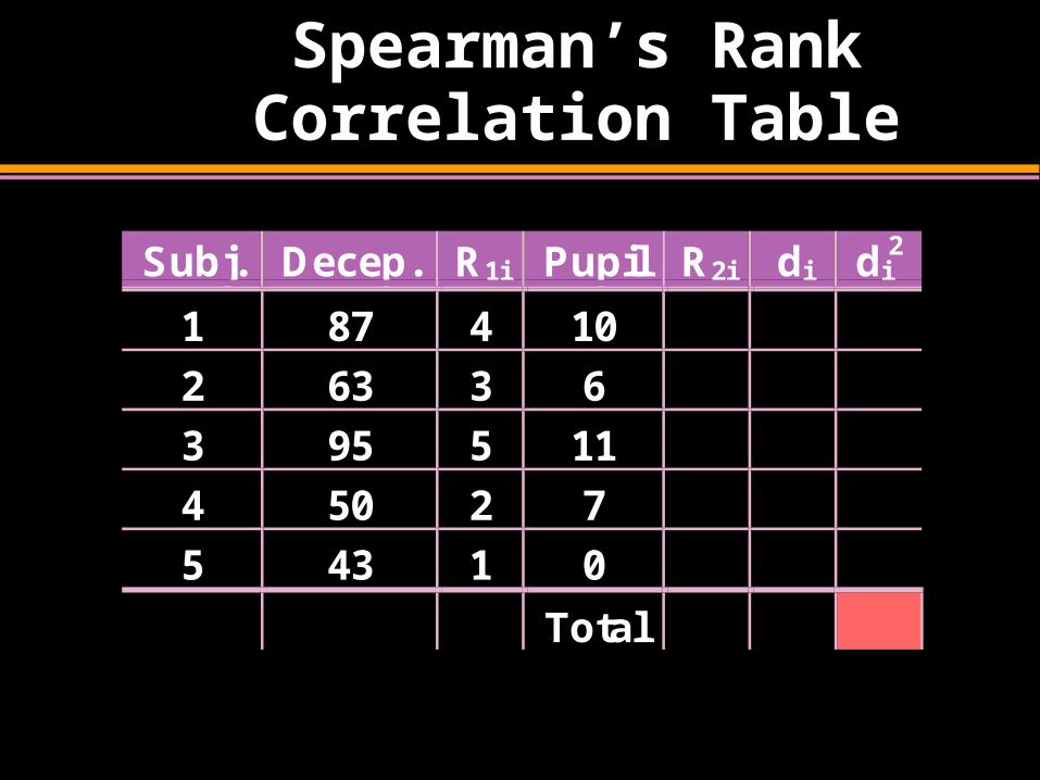
Spearman’s Rank Correlation Table
Subj. Decep. R1i Pupil R2i di di2
1 87 4 10
2 63 3 6
3 95 5 11
4 50 2 7
5 43 1 0
Total
Spearman’s Rank Correlation Table
Subj. Decep. R1i Pupil R2i di di2
1 87 4 10 4
2 63 3 6 2
3 95 5 11 5
4 50 2 7 3
5 43 1 0 1
Total
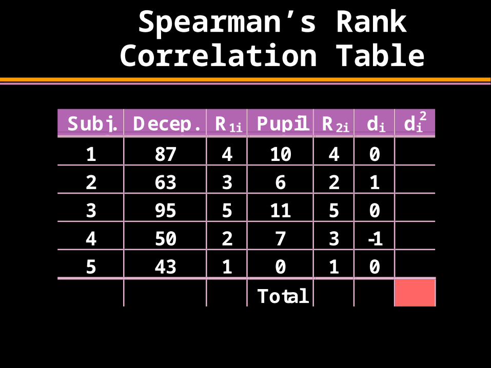
Spearman’s Rank Correlation Table
Subj. Decep. R1i Pupil R2i di di2
1 87 4 10 4 0
2 63 3 6 2 1
3 95 5 11 5 0
4 50 2 7 3 -1
5 43 1 0 1 0
Total
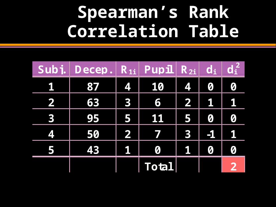
Spearman’s Rank Correlation Table
Subj. Decep. R1i Pupil R2i di di2
1 87 4 10 4 0 0
2 63 3 6 2 1 1
3 95 5 11 5 0 0
4 50 2 7 3 -1 1
5 43 1 0 1 0 0
Total 2
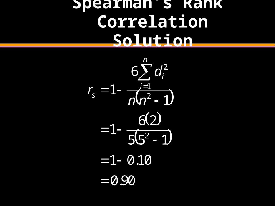
Spearman’s Rank Correlation Solution
90.0
10.01
155
261
1
61
2
21
2
nn
dr
n
ii
s
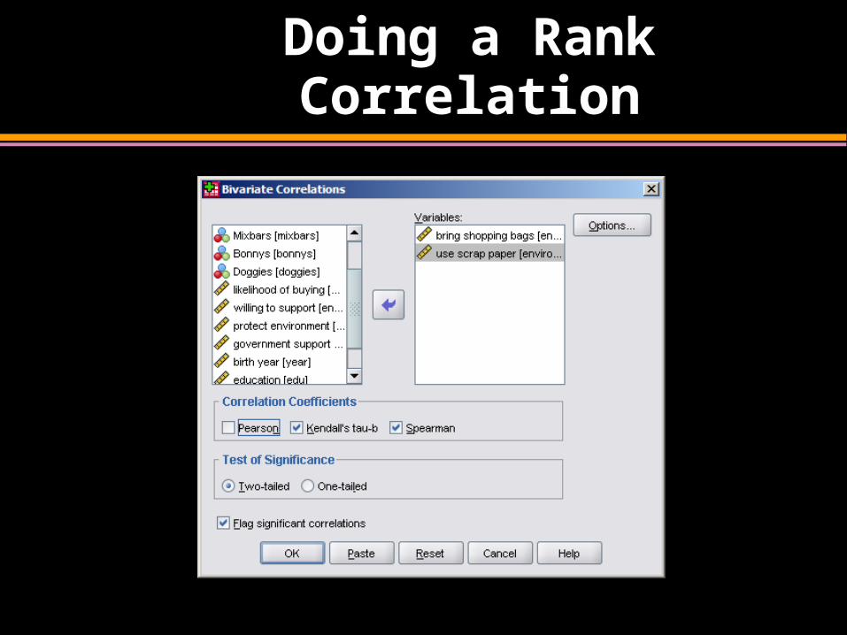
Doing a Rank Correlation
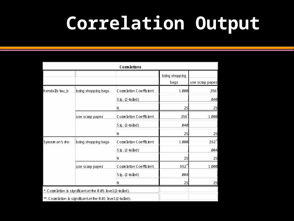
Correlation Output
Correlations
bring shopping
bags use scrap paper
Kendall's tau_b bring shopping bags Correlation Coefficient 1.000 .356*
Sig. (2-tailed) . .040
N 25 25
use scrap paper Correlation Coefficient .356* 1.000
Sig. (2-tailed) .040 .
N 25 25
Spearman's rho bring shopping bags Correlation Coefficient 1.000 .552**
Sig. (2-tailed) . .004
N 25 25
use scrap paper Correlation Coefficient .552** 1.000
Sig. (2-tailed) .004 .
N 25 25
*. Correlation is significant at the 0.05 level (2-tailed).
**. Correlation is significant at the 0.01 level (2-tailed).
20-88
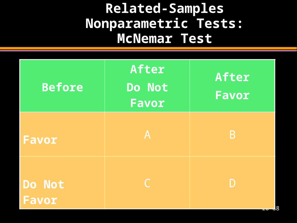
Related-Samples Nonparametric Tests:
McNemar Test
BeforeAfter
Do Not FavorAfterFavor
Favor A B
Do Not Favor C D
20-89
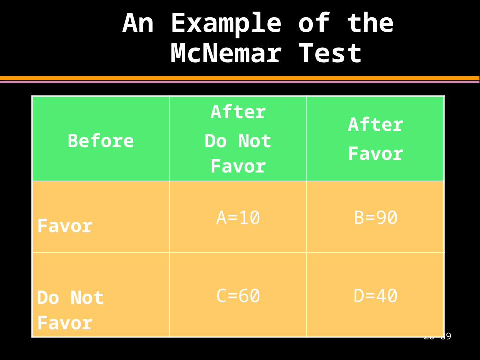
An Example of the McNemar Test
BeforeAfter
Do Not FavorAfterFavor
Favor A=10 B=90
Do Not Favor C=60 D=40
Chi-square Test
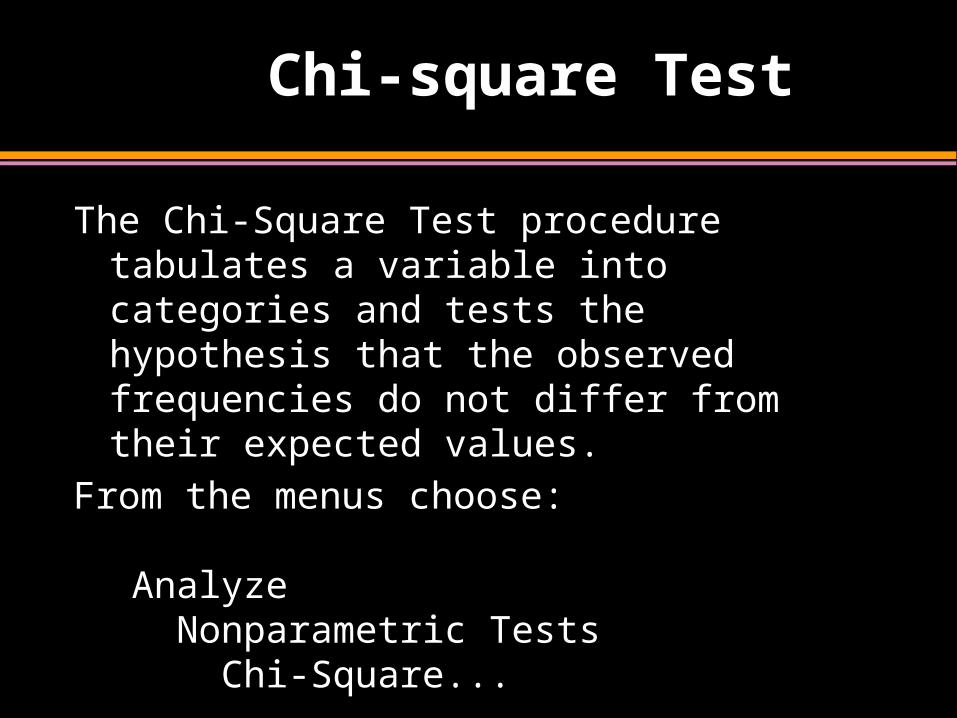
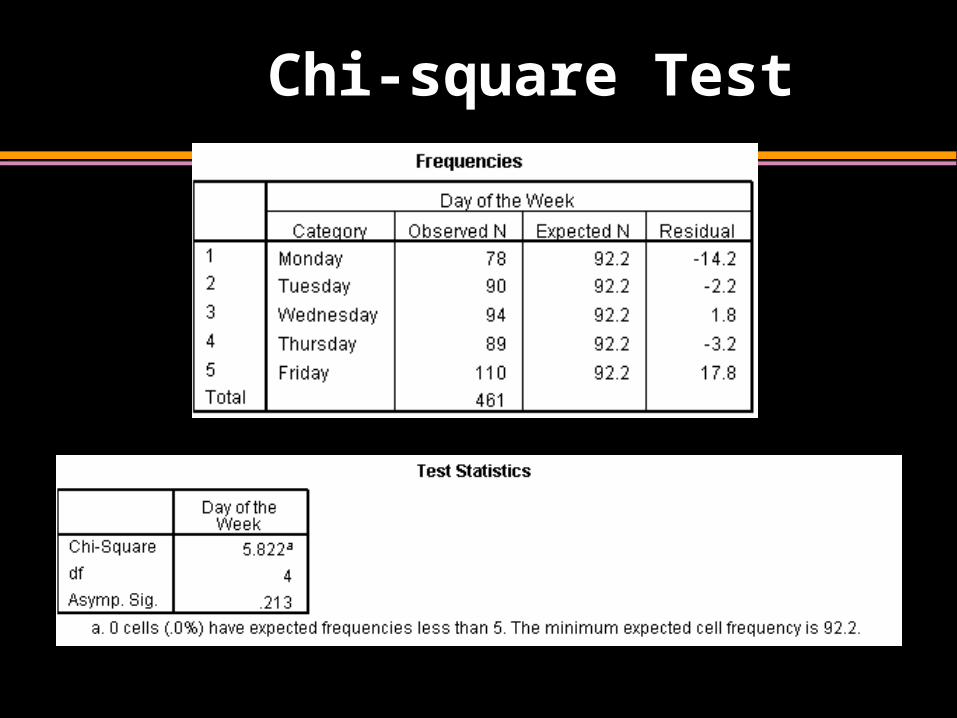
The Chi-Square Test procedure tabulates a variable into categories and tests the hypothesis that the observed frequencies do not differ from their expected values.
From the menus choose:
Analyze Nonparametric Tests Chi-Square...
Chi-square Test
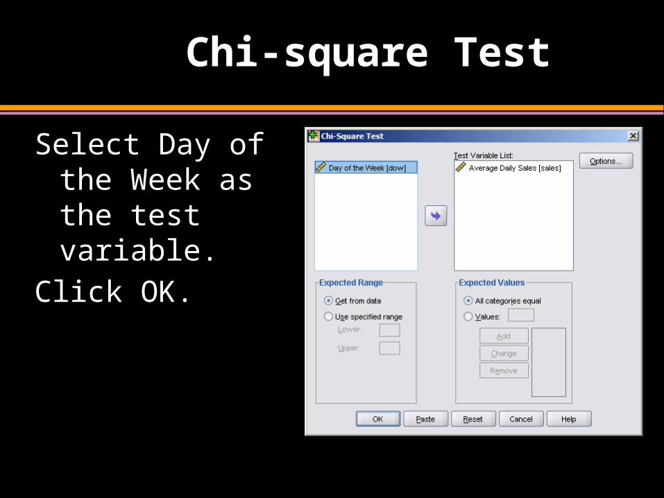
Select Day of the Week as the test variable.
Click OK.
Chi-square Test
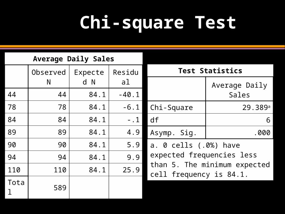
Average Daily Sales
Observed N Expected N Residual
44 44 84.1 -40.1
78 78 84.1 -6.1
84 84 84.1 -.1
89 89 84.1 4.9
90 90 84.1 5.9
94 94 84.1 9.9
110 110 84.1 25.9
Total589
Test Statistics
Average Daily Sales
Chi-Square 29.389a
df 6
Asymp. Sig. .000
a. 0 cells (.0%) have expected frequencies less than 5. The minimum expected cell frequency is 84.1.
Chi-square Test
Chi-square Test
End of Chapter
95


![Untitled-1 [bagelcafenyc.com]€¦ · Tuna Salad Low-Fat Vegetable Tuna Salad Spicy Tuna Salad Egg Salad Egg White Salad Baked Salmon Salad White Fish Salad Chopped Liver Chicken](https://img.pdfslide.us/doc/110x75/5fffad90e43d8b65ef058ba7/untitled-1-tuna-salad-low-fat-vegetable-tuna-salad-spicy-tuna-salad-egg-salad.jpg)