Nonparametric Modeling, Learning, and Inference - Brown University

Applied Bayesian Nonparametrics

1. Models & Inference

Tutorial at CVPR 2012Erik Sudderth Brown University

Additional detail & citations in background chapter: E. B. Sudderth, Graphical Models for Visual Object Recognition and Tracking, PhD Thesis, MIT, 2006.

Applied

Bayesian

Nonparametric

Statistics Learning probabilistic models of visual data.

Clustering & features, space & time, mostly unsupervised.

Complex data motivates models of unbounded complexity. We often need to learn the structure of the model itself.

Not no parameters! Models with infinitely many parameters. Distributions on uncertain functions, distributions, !

Focus on those models which are most useful in practice. To understand those models, we’ll start with theory!

Applied BNP: Part I •! Review of parametric Bayesian models

!! Finite mixture models !!Beta and Dirichlet distributions

•! Canonical Bayesian nonparametric (BNP) model families !!Dirichlet & Pitman-Yor processes for infinite clustering !!Beta processes for infinite feature induction

•! Key representations for BNP learning !! Infinite-dimensional stochastic processes !!Stick-breaking constructions !!Partitions and Chinese restaurant processes !! Infinite limits of finite, parametric Bayesian models

•! Learning and inference algorithms !!Representation and truncation of infinite models !!MCMC methods and Gibbs samplers !!Variational methods and mean field

Coffee Break

Applied BNP: Part II

Bayes Rule (Bayes Theorem) unknown parameters (many possible models)

observed data available for learning

prior distribution (domain knowledge)

likelihood function (measurement model)

posterior distribution (learned information)

θD

p(θ)

p(D | θ)p(θ | D)

p(θ,D) = p(θ)p(D | θ) = p(D)p(θ | D)

∝ p(D | θ)p(θ)

p(θ | D) =p(θ,D)

p(D)=

p(D | θ)p(θ)∑θ′∈Θ p(D | θ′)p(θ′)

Gaussian Mixture Models •! Observed feature vectors: •! Hidden cluster labels:

•! Hidden mixture means:

•! Hidden mixture covariances:

•! Hidden mixture probabilities:

xi ∈ Rd, i = 1, 2, . . . , N

µk ∈ Rd, k = 1, 2, . . . ,K

zi ∈ {1, 2, . . . ,K}, i = 1, 2, . . . , N

Σk ∈ Rd×d, k = 1, 2, . . . ,K

πk,

K∑

k=1

πk = 1

•! Gaussian mixture marginal likelihood:

p(xi | π, µ,Σ) =K∑

zi=1

πziN (xi | µzi ,Σzi)

p(xi | zi,π, µ,Σ) = N (xi | µzi ,Σzi)

Gaussian Mixture Models Mixture of 3 Gaussian

Distributions in 2D Contour Plot of Joint Density,

Marginalizing Cluster Assignments

0 0.2 0.4 0.6 0.8 1

0.25

0.3

0.35

0.4

0.45

0.5

0.55

0.6

0.65

0.7

0.75

0 0.1 0.2 0.3 0.4 0.5 0.6 0.7 0.8 0.9

0.25

0.3

0.35

0.4

0.45

0.5

0.55

0.6

0.65

0.7

p(xi | π, µ,Σ) =K∑

zi=1



Gaussian Mixture Models

Surface Plot of Joint Density, Marginalizing Cluster Assignments

Clustering with Gaussian Mixtures

C. Bishop, Pattern Recognition & Machine Learning

(a)

0 0.5 1

0

0.5

1 (b)

0 0.5 1

0

0.5

1

Complete Data Labeled by True Cluster Assignments

Incomplete Data: Points to be Clustered

Inference Given Cluster Parameters

(b)

0 0.5 1

0

0.5

1

Posterior Probabilities of Assignment to Each Cluster

Incomplete Data: Points to be Clustered

(c)

0 0.5 1

0

0.5

1

rik = p(zi = k | xi,π, θ) =πkp(xi | θk)∑K�=1 π�p(xi | θ�)

Learning Binary Probabilities Bernoulli Distribution: Single toss of a (possibly biased) coin

0 ≤ θ ≤ 1

Xi ∼ Ber(θ), i = 1, . . . , N

•! Suppose we observe N samples from a Bernoulli distribution with unknown mean:

•! What is the maximum likelihood parameter estimate?

p(x1, . . . , xN | θ) = θN1(1− θ)N0

Ber(x | θ) = θI(x=1)(1− θ)I(x=0)

θ̂ = argmaxθ

log p(x | θ) = N1

N

Beta Distributions

Probability density function: x ∈ [0, 1]

Γ(k) = (k − 1)!

Γ(x+ 1) = xΓ(x)

Beta Distributions

E[x] =a

a+ bV[x] =

ab

(a+ b)2(a+ b+ 1)

Mode[x] = arg maxx∈[0,1]

Beta(x | a, b) = a− 1

(a− 1) + (b− 1)

Bayesian Learning of Probabilities Bernoulli Likelihood: Single toss of a (possibly biased) coin

0 ≤ θ ≤ 1Ber(x | θ) = θI(x=1)(1− θ)I(x=0)

p(x1, . . . , xN | θ) = θN1(1− θ)N0

Beta Prior Distribution:

p(θ) = Beta(θ | a, b) ∝ θa−1(1− θ)b−1

p(θ | x) ∝ θN1+a−1(1− θ)N0+b−1 ∝ Beta(θ | N1 + a,N0 + b)

Posterior Distribution:

•! This is a conjugate prior, because posterior is in same family •! Estimate by posterior mode (MAP) or mean (preferred)

Sequence of Beta Posteriors

0 0.2 0.4 0.6 0.8 1

0

1

2

3

4

5

6

7

8

9

10

truth

n=5

n=50

n=100

Murphy 2012

Multinomial Simplex

Learning Categorical Probabilities Categorical Distribution: Single roll of a (possibly biased) die

Cat(x | θ) =K∏

k=1

θxk

k X = {0, 1}K ,

K∑

k=1

xk = 1

p(x1, . . . , xN | θ) =∏K

k=1 θNk

k

•! If we have Nk observations of outcome k in N trials:

•! The maximum likelihood parameter estimates are then:

•! Will this produce sensible predictions when K is large? For nonparametric models we let K approach infinity!

θ̂ = argmaxθ

log p(x | θ) θ̂k =Nk

N

Dirichlet Distributions

0

0.5

1

0

0.5

10

5

10

15

20

25

α=10.00

p

0

0.5

0

0.5

10

5

10

15

α=0.10

p

Moments:

Marginal Distributions:

Dirichlet Probability Densities

Dirichlet Samples

Dir(θ | 0.1, 0.1, 0.1, 0.1, 0.1) Dir(θ | 1.0, 1.0, 1.0, 1.0, 1.0)

Bayesian Learning of Probabilities

Dirichlet Prior Distribution:

Posterior Distribution:

•! This is a conjugate prior, because posterior is in same family

Categorical Distribution: Single roll of a (possibly biased) die

Cat(x | θ) =K∏

k=1

θxk

k X = {0, 1}K ,

K∑

k=1

xk = 1

p(x1, . . . , xN | θ) =∏K

k=1 θNk

k

p(θ) = Dir(θ | α) ∝K∏

k=1

θαk−1k

p(θ | x) ∝K∏

k=1

θNk+αk−1k ∝ Dir(θ | N1 + α1, . . . , NK + αK)

Directed Graphical Models Chain rule implies that any joint distribution equals:

Directed graphical model implies a restricted factorization:

pa(t) → parents with edges pointing to node t

nodes → random variables

Valid for any directed acyclic graph (DAG): equivalent to dropping conditional

dependencies in standard chain rule

Plates: Learning with Priors

•! Boxes, or plates, indicate replication of variables •! Variables which are observed, or fixed, are often shaded •! Prior distributions may themselves have hyperparameters λ

Gaussian Mixture Models

0 0.2 0.4 0.6 0.8 1

0.25

0.3

0.35

0.4

0.45

0.5

0.55

0.6

0.65

0.7

0.75

p(xi | π, µ,Σ) =K∑

zi=1



Finite Bayesian Mixture Models

(a)

•! Cluster frequencies: Symmetric Dirichlet

0

0.5

1

0

0.5

10

5

10

15

•! Cluster shapes: Any valid prior on chosen family (e.g., Gaussian mean & covariance)

•! Data: Assign each data item to a cluster, and sample from that cluster’s likelihood

zi ∼ Cat(π)

xi ∼ F (θzi)

Generative Gaussian Mixture Samples

•! Gaussian with known variance: Gaussian prior on mean •! Gaussian with unknown mean & variance: normal inverse-Wishart

Learning is simplest with conjugate priors on cluster shapes:

Mixtures as Discrete Measures

Θ

Θ

Θ

XToy visualization: 1D Gaussian mixture with unknown cluster

means and fixed variance

G(θ) =

K∑

k=1

πkδθk(θ)

•! Define mixture via a discrete probability measure on cluster parameters:

δθk atom, point mass, Dirac delta

•! Generate data via repeated draws G:

θ̄i = θzi

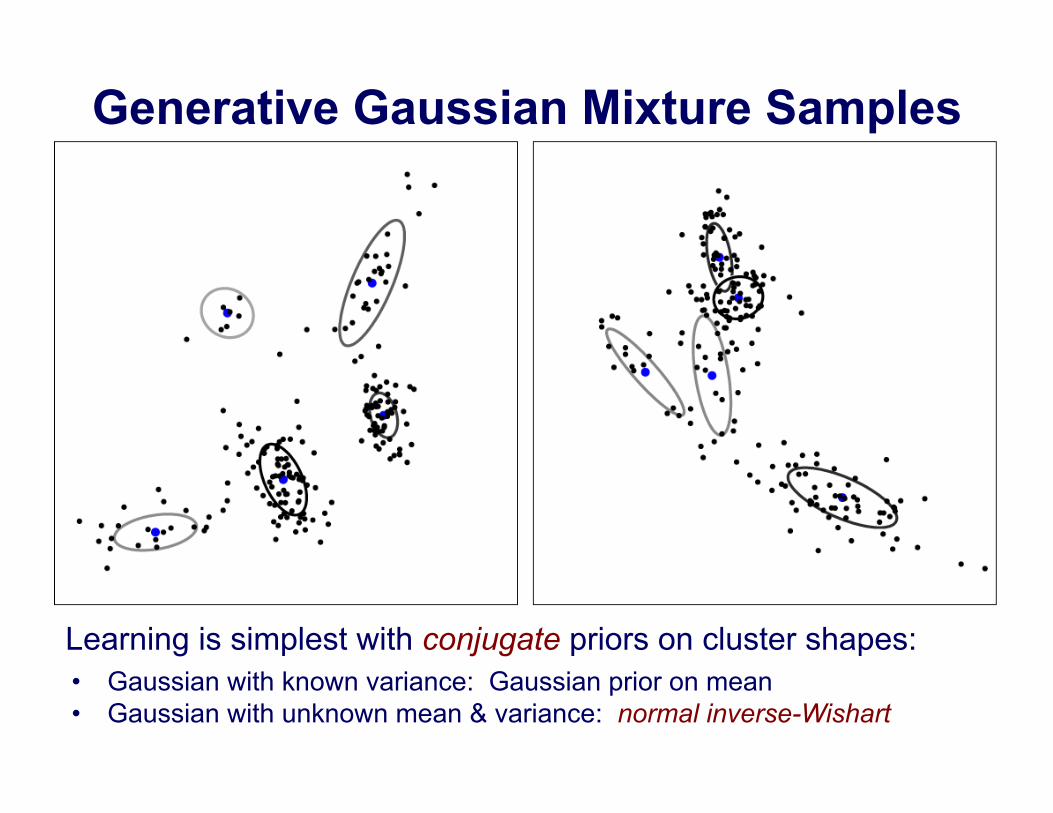
Mixtures Induce Partitions

(a)

zi ∼ Cat(π)

•! If our goal is clustering, the output grouping is defined by assignment indicator variables:

•! The number of ways of assigning N data points to K mixture components is KN

K ≥ N•! If this is much larger than the number of ways of partitioning that data:

33 = 27N=3: 5 partitions versus

Mixtures Induce Partitions

zi ∼ Cat(π)

•! If our goal is clustering, the output grouping is defined by assignment indicator variables:

•! The number of ways of assigning N data points to K mixture components is KN

K ≥ N•! If this is much larger than the number of ways of partitioning that data:

N=5: 52 partitions versus 55 = 3125

t t o s

ns versus 55 3

Courtesy Wikipedia

For any clustering, there is a unique partition, but many ways to

label that partition’s blocks.

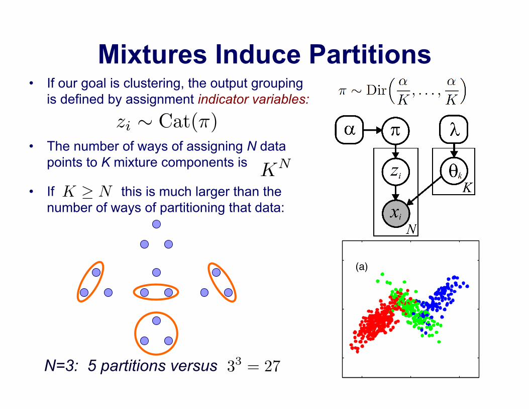
Dirichlet Process Mixtures The Dirichlet Process (DP) A distribution on countably infinite

discrete probability measures. Sampling yields a Polya urn.

Infinite Mixture Models As an infinite limit of finite

mixtures with Dirichlet weight priors

Stick-Breaking An explicit construction

for the weights in DP realizations

Chinese Restaurant Process (CRP) The distribution on

partitions induced by a DP prior



Dirichlet Process Mixtures

Nonparametric Clustering

•! Large Support: All partitions of the data, from one giant cluster to N singletons, have positive probability under prior

•! Exchangeable: Partition probabilities are invariant to permutations of the data

•! Desirable: Good asymptotics, computational tractability, flexibility and ease of generalization!

Clusters, arbitrarily ordered

Obs

erva

tions

, arb

itrar

ily o

rder

ed Ghahramani,

BNP 2009

Chinese Restaurant Process (CRP) •! Visualize clustering as a sequential process of customers

sitting at tables in an (infinitely large) restaurant: customers observed data to be clustered

tables distinct blocks of partition, or clusters

•! The first customer sits at a table. Subsequent customers randomly select a table according to:

number of tables occupied by the first N customers

number of customers seated at table k

k̄ a new, previously unoccupied table

K

Nk

α positive concentration parameter

Chinese Restaurant Process (CRP) ( )

CRPs & Exchangeable Partitions

•! The probability of a seating arrangement of N customers is independent of the order they enter the restaurant:

p(z1, . . . , zN | α) = Γ(α)

Γ(N + α)αK

K∏

k=1

Γ(Nk)

1

1 + α· 1

2 + α· · · 1

N − 1 + α=

Γ(α)

Γ(N + α)normalization constants

α

1 · 2 · · · (Nk − 1) = (Nk − 1)! = Γ(Nk)

first customer to sit at each table other customers joining each table

•! The CRP is thus a prior on infinitely exchangeable partitions

De Finetti’s Theorem •! Finitely exchangeable random variables satisfy:

•! A sequence is infinitely exchangeable if every finite subsequence is exchangeable

•! Exchangeable variables need not be independent, but always have a representation with conditional independencies:

An explicit construction is useful in hierarchical modeling!

De Finetti’s Directed Graph

What distribution underlies the infinitely exchangeable CRP?





Dirichlet Processes

•! Given a base measure (distribution) H & concentration parameter •! Then for any finite partition

the distribution of the measure of those cells is Dirichlet:

Ferguson 1973

Base Measure

α > 0

Dirichlet Processes

•! Marginalization properties of finite Dirichlet distributions satisfy Kolmogorov’s extension theorem for stochastic processes:

Ferguson 1973

Base Measure

DP Posteriors and Conjugacy

•! Does the posterior distribution of G have a tractable form? •! For any partition, the posterior mean given N observations is

G ∼ DP(α, H) θ̄i ∼ G, i = 1, . . . , N

•! In fact, the posterior distribution is another Dirichlet process, with mean that depends on the data’s empirical distribution:

DPs and Polya Urns

!! Consider an urn containing ! pounds of very tiny, colored sand (the space of possible colors is ")

!! Take out one grain of sand, record its color as !! Put that grain back, add 1 extra pound of that color !! Repeat this process!

θ̄1

•! Can we simulate observations without constructing G? •! Yes, by a variation on the classical balls in urns analogy:

G ∼ DP(α, H) θ̄i ∼ G, i = 1, . . . , N







A Stick-Breaking Construction

0 1

concentration parameter

•! Dirichlet process realizations are discrete with probability one:

G ∼ DP(α, H) G(θ) =

∞∑

k=1

πkδθk(θ)

Sethuraman 1994

•! Cluster shape parameters drawn from base measure: θk ∼ H

•! Cluster weights drawn from a stick-breaking process:

Dirichlet Stick-Breaking E[βk] =

1

1 + αβk ∼ Beta(1,α)

DPs and Stick Breaking









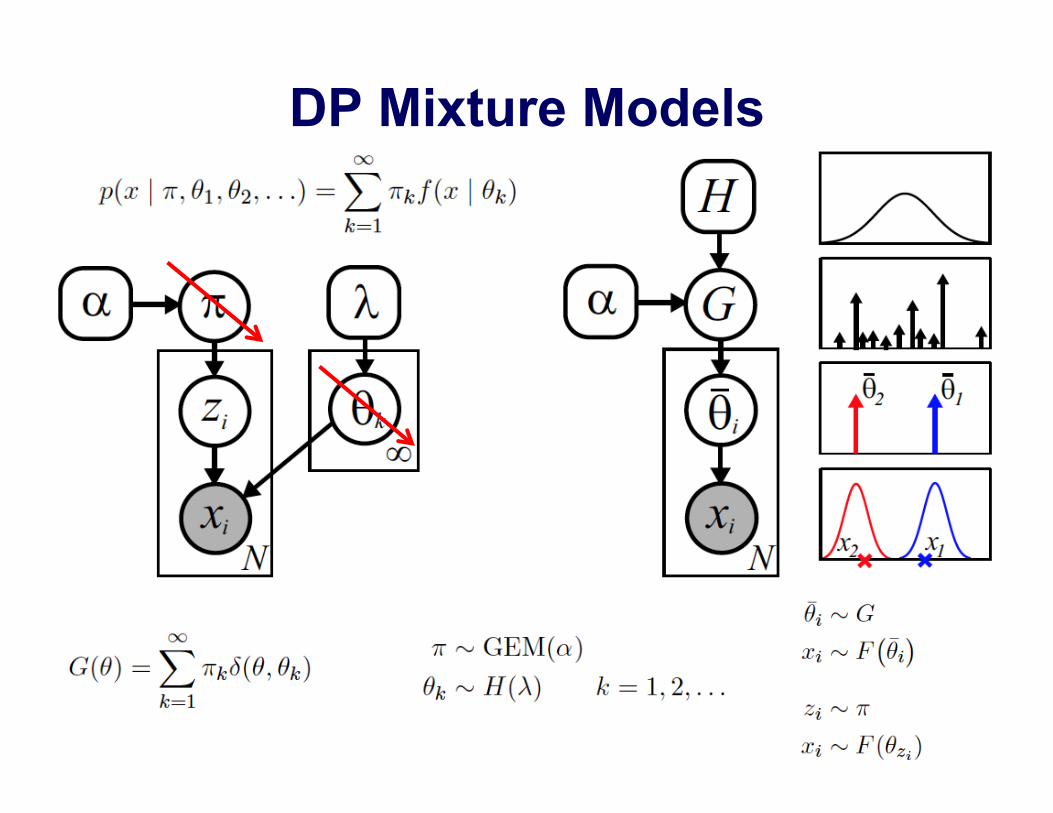
DP Mixture Models

G ∼ DP(α, H)

θ̄i ∼ Gxi ∼ F (θ̄i)

G(θ) =

∞∑

k=1

πkδθk(θ)

zi ∼ Cat(π)

xi ∼ F (θzi)

θk ∼ H(λ)π ∼ Stick(α)

•! Stick-breaking: Explicit size-biased sampling of weights •! Chinese restaurant process: Indicator sequence •! Polya urn: Corresponding parameter sequence

z1, z2, z3, . . .θ̄1, θ̄2, θ̄3, . . .

π

Samples from DP Mixture Priors

N=50


N=200


N=1000

Finite versus DP Mixtures tu es

π ∼ Stick(α)

zi ∼ Cat(π)

xi ∼ F (θzi)

Finite Mixture DP Mixture

GK(θ) =

K∑

k=1

πkδθk(θ)

THEOREM: For any measureable function f, as K → ∞

G ∼ DP(α, H)

θk ∼ H

Finite versus CRP Partitions a t t o s

π ∼ Stick(α)

zi ∼ Cat(π)

Finite Mixture DP Mixture

Chinese Restaurant Process:

p(z1, . . . , zN | α) = Γ(α)

Γ(N + α)

( α

K

)K+K+∏

k=1

Nk−1∏

j=1

(j +

α

K

)

p(z1, . . . , zN | α) = Γ(α)

Γ(N + α)αK+

K+∏

k=1

(Nk − 1)!

K+ number of blocks in cluster

Finite Dirichlet:

•! Probability of Dirichlet indicators approach zero as •! Probability of Dirichlet partition approaches CRP as K → ∞









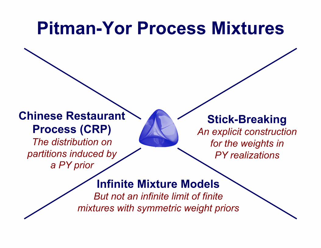
Pitman-Yor Process Mixtures

Infinite Mixture Models But not an infinite limit of finite

mixtures with symmetric weight priors


for the weights in PY realizations


partitions induced by a PY prior

Pitman-Yor Processes The Pitman-Yor process defines a distribution on

infinite discrete measures, or partitions

Dirichlet process:

0 1

Dirichlet Stick-Breaking

All stick indices

Pitman-Yor Stick-Breaking

Chinese Restaurant Process (CRP) customers observed data to be clustered

tables distinct blocks of partition, or clusters •! Partitions sampled from the PY process can be generated

via a generalized CRP, which remains exchangeable •! The first customer sits at a table. Subsequent customers

randomly select a table according to:

number of tables occupied by the first N customers

number of customers seated at table k

k̄ a new, previously unoccupied table

K

Nk

discount & concentration parameters 0 ≤ a < 1, b > −a

p(zN+1 = z | z1, . . . , zN ) =1

b+N

(K∑

k=1

(Nk − a)δ(z, k) + (b+Ka)δ(z, k̄)

)

Human Image Segmentations

Labels for more than 29,000 segments in 2,688 images of natural scenes

Statistics of Human Segments How many objects are in this image?

Many Small

Objects

Some Large

Objects

Object sizes follow a power law


Statistics of Semantic Labels

sky trees

person

lichen

rainbow wheelbarrow

waterfall


How frequent are text region labels?

Why Pitman-Yor?

Jim Pitman

Marc Yor

Generalizing the Dirichlet Process !!Distribution on partitions leads to a

generalized Chinese restaurant process

! Special cases of interest in probability: Markov chains, Brownian motion, !

Power Law Distributions DP PY

Number of unique clusters in N observations

Heaps Law:

Size of sorted cluster weight k

Goldwater, Griffiths, & Johnson, 2005 Teh, 2006

Natural Language Statistics

Zipf s Law:

An Aside: Toy Dataset Bias

! !"# $ $"# % %"# & &"# ' '"# #!

!"#

$

$"#

%

%"#

&

&"#

'

'"#

#()*+,-.-/01+234+

! !"# $ $"# % %"# & &"# ' '"# #!

!"#

$

$"#

%

%"#

&

&"#

'

'"#

#0)(35(67500+,-&-/01+234+

! !"# $ $"# % %"# & &"# ' '"# #!

!"#

$

$"#

%

%"#

&

&"#

'

'"#

#8914/0916+,-%-/01+234+

! !"# $ $"# % %"# & &"# ' '"# #!

!"#

$

$"#

%

%"#

&

&"#

'

'"#

#+:1);;03+,-'-/01+234+

! !"# $ $"# % %"# & &"# ' '"# #!

!"#

$

$"#

%

%"#

&

&"#

'

'"#

#2<9/)4/03+,-%-/01+234+

! !"# $ $"# % %"# & &"# ' '"# #!

!"#

$

$"#

%

%"#

&

&"#

'

'"#

#2=433/)4/03+ >9)(36,-%-/01+234+

- - - - - -Ng, Jordan, & Weiss, NIPS 2001

Pitman-Yor Process Mixtures

Infinite Mixture Models But not an infinite limit of finite

mixtures with symmetric weight priors


for the weights in PY realizations


partitions induced by a PY prior

Dirichlet processes and finite Dirichlet distributions do not produce

heavy-tailed, power law distributions

Latent Feature Models

•! Latent feature modeling: Each group of observations is associated with a subset of the possible latent features

•! Factorial power: There are 2K combinations of K features, while accurate mixture modeling may require many more clusters

•! Question: What is the analog of the DP for feature modeling?

Binary matrix indicating feature presence/absence

Depending on application, features can be associated with any parameter value of interest

Nonparametric Binary Features The Beta Process (BP)

A Levy process whose realizations are countably infinite collections of

atoms, with mass between 0 and 1.

Infinite Feature Models As an infinite limit of a finite

beta-Bernoulli binary feature model


for the feature frequencies in BP realizations

Indian Buffet Process (IBP)

The distribution on sparse binary matrices

induced by a BP

Poisson Distribution for Counts

X = {0, 1, 2, 3, . . .}

Poi(x | θ) = e−θ θx

x!θ > 0

Indian Buffet Process (IBP) •! Visualize feature assignment as a sequential process of

customers sampling dishes from an (infinitely long) buffet: customers observed data to be modeled

dishes binary features to be selected •! The first customer chooses dishes, •! Subsequent customer i randomly samples each previously

tasted dish k with probability

•! That customer also samples new dishes number of previous customers to sample dish k

Poisson(α)

fik ∼ Ber(mk

i

)

Poisson(α/i)

mk

α > 0

Binary Feature Realizations

•! IBP is exchangeable, up to a permutation of the order with which dishes are listed in the binary feature matrix

•! Clustering models like the DP have one “feature” per customer •! The number of features sampled at least once is

y

Ghahramani, BNP 2009

O(α logN)

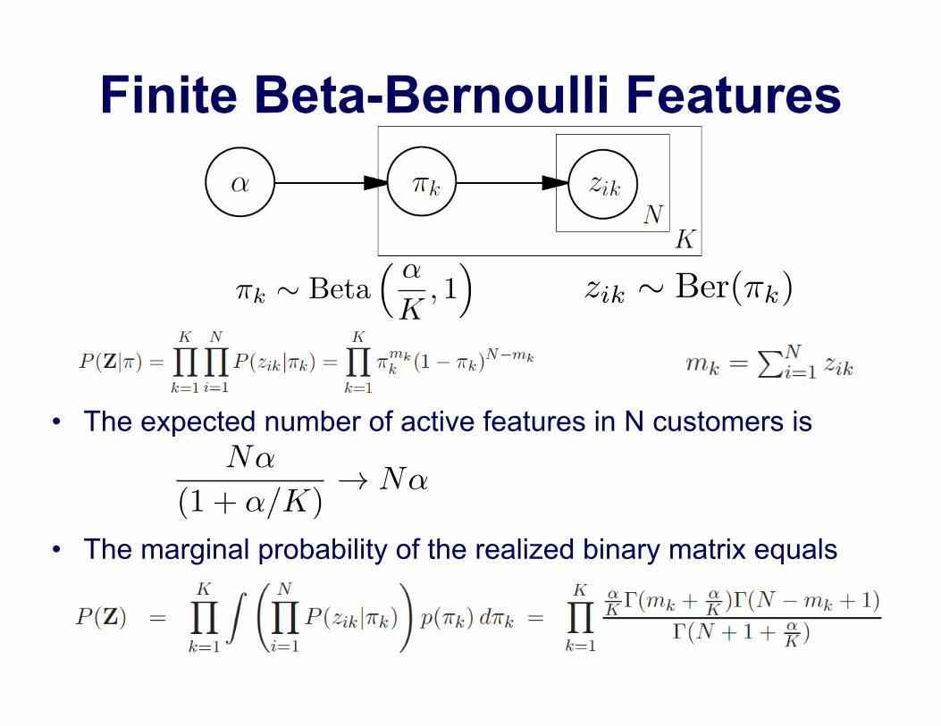
Finite Beta-Bernoulli Features

πk ∼ Beta( α

K, 1)

zik ∼ Ber(πk)

•! The expected number of active features in N customers is Nα

(1 + α/K)→ Nα

•! The marginal probability of the realized binary matrix equals

Beta-Bernoulli and the IBP •! We can show that the limit of the finite beta-Bernoulli model,

and the IBP, produce the same distribution on left-ordered-form equivalence classes of binary matrices:

•! Poisson distribution in IBP arises from the law of rare events: •! Flip K coins with probability of coming up heads •! As the distribution of the number of total heads

approaches Poisson(α)

α/KK → ∞

Nonparametric Binary Features The Beta Process (BP)

A Levy process whose realizations are countably infinite collections of

atoms, with mass between 0 and 1.

Infinite Feature Models As an infinite limit of a finite

beta-Bernoulli binary feature model


for the feature frequencies in BP realizations

Indian Buffet Process (IBP)

The distribution on sparse binary matrices

induced by a BP

Extensions: Additional control over feature sharing, power laws!

Nonparametric Learning

Finite Bayesian Models Set finite model order to be larger

than expected number of clusters or features.

Stick-Breaking Truncate stick-breaking

to produce provably accurate approximation.

CRP & IBP Tractably learn via finite

summaries of true, infinite model.

Infinite Stochastic Processes Conceptually useful, but usually

impractical or impossible for learning algorithms.

Markov Chain Monte Carlo

•! At each time point, state is a configuration of all the variables in the model: parameters, hidden variables, etc. •! We design the transition distribution so that

the chain is irreducible and ergodic, with a unique stationary distribution

z(0) z(1) z(2) z(t+1) ∼ q(z | z(t))

z(t)

q(z | z(t))

p∗(z)

p∗(z) =

∫

Zq(z | z′)p∗(z′) dz′

•! For learning, the target equilibrium distribution is usually the posterior distribution given data x: •! Popular recipes: Metropolis-Hastings and Gibbs samplers

p∗(z) = p(z | x)

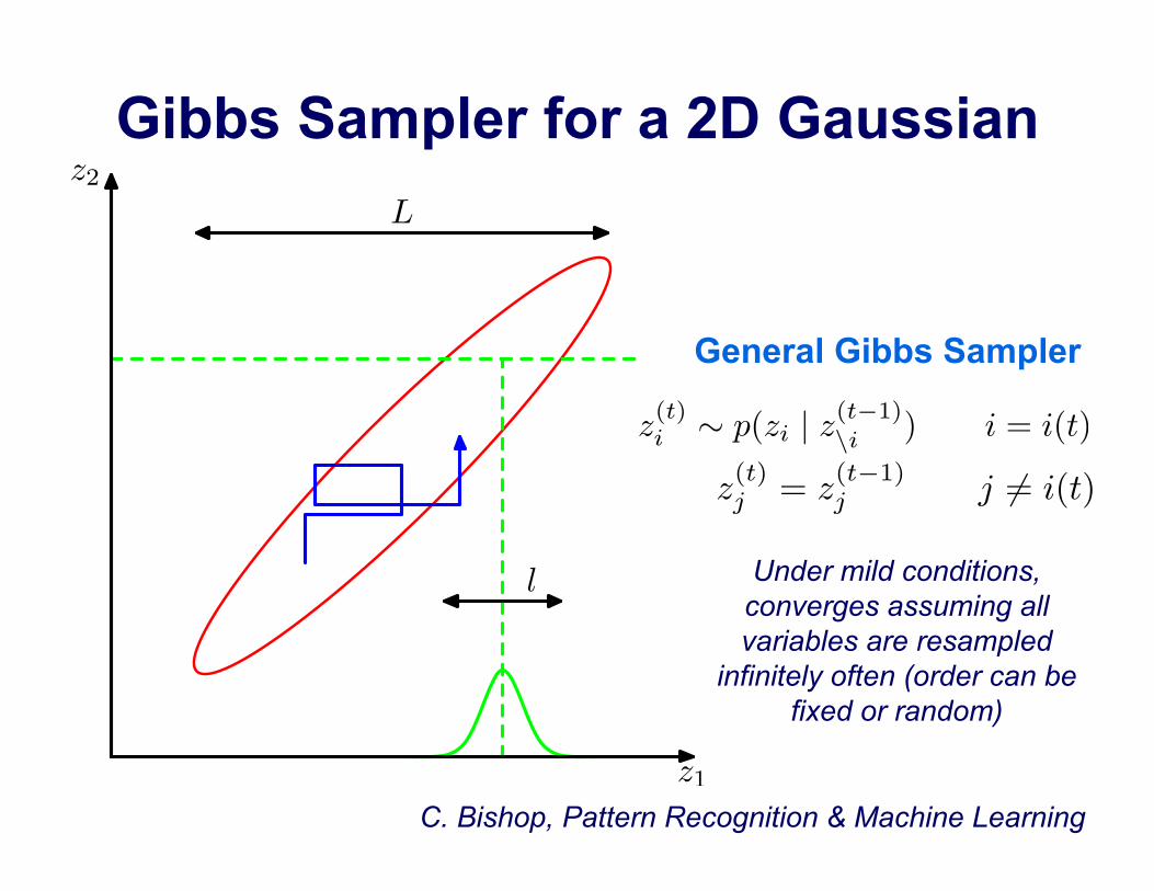
Gibbs Sampler for a 2D Gaussian

C. Bishop, Pattern Recognition & Machine Learning z1

z2

L

l

z(t)i ∼ p(zi | z(t−1)

\i ) i = i(t)

z(t)j = z

(t−1)j j �= i(t)

Under mild conditions, converges assuming all variables are resampled

infinitely often (order can be fixed or random)

General Gibbs Sampler

Finite Mixture Gibbs Sampler

Most basic approach: Sample z, #, $%

Standard Finite Mixture Sampler

Standard Sampler: 2 Iterations



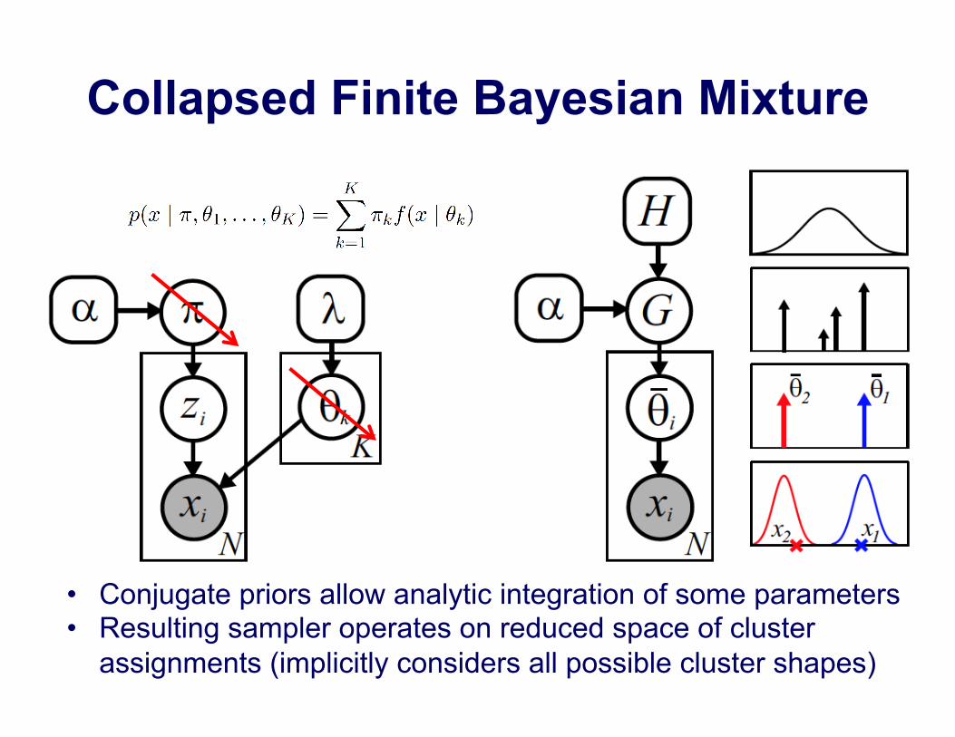
Collapsed Finite Bayesian Mixture

•! Conjugate priors allow analytic integration of some parameters •! Resulting sampler operates on reduced space of cluster

assignments (implicitly considers all possible cluster shapes)

Collapsed Finite Mixture Sampler

Standard versus Collapsed Samplers

DP Mixture Models

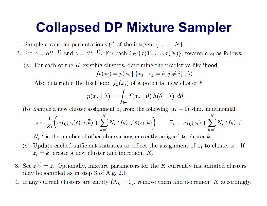
Collapsed DP Mixture Sampler

Collapsed DP Sampler: 2 Iterations



DP versus Finite Mixture Samplers

DP Posterior Number of Clusters

Bayesian Ockham’s Razor

William of Ockham

Plurality must never be posited without necessity.

Dm

θ

data

model

parameters

Even with uniform p(m), marginal likelihood provides a model selection bias

Example: Is this coin fair? M0: Tosses are from a fair coin: M1: Tosses are from a coin of unknown bias:

θ = 1/2

θ ∼ Unif(0, 1)

Marginal Likelihoods

Number of heads in N=5 tosses

M1

M0

•! ML: Always prefer M1 •! Bayes: Unbalanced counts

are much more likely with a biased coin, so favor M1

•! Bayes: Balanced counts only happen with some biased coins, so favor M0

Variational Approximations

(Multiply by one)

(Jensen’s inequality)

•! Minimizing KL divergence maximizes a likelihood bound •! Variational EM algorithms, which maximize for q(x) within

some tractable family, retain BNP model selection behavior

Mean Field for DP Mixtures

•! Truncate stick-breaking at some upper bound K on the true number of occupied clusters:

•! Priors encourage assigning data to fewer than K clusters

k = 1, . . . ,K − 1

πK = 1−K−1∑

k=1

πk

Blei & Jordan 2006

MCMC & Variational Learning

Finite Bayesian Models Set finite model order to be larger

than expected number of clusters or features.

Stick-Breaking Truncate stick-breaking

to produce provably accurate approximation.

CRP & IBP Tractably learn via finite

summaries of true, infinite model.

Infinite Stochastic Processes Conceptually useful, but usually

impractical or impossible for learning algorithms.

Applied BNP: Part II

Documents

Nonparametric Modeling, Learning, and Inference - Brown University