Nonparametric graphical model for counts

Journal of Machine Learning Research 21 (2020) 1-22 Submitted 5/19; Published 12/20

Nonparametric graphical model for counts

Arkaprava Roy [email protected] of BiostatisticsUniversity of FloridaGainesville, FL 32611, USA

David B Dunson [email protected]

Department of Statistics

Duke University

Durham, NC 27708-0251, USA

Editor: Robert McCulloch

Abstract

Although multivariate count data are routinely collected in many application areas, thereis surprisingly little work developing flexible models for characterizing their dependencestructure. This is particularly true when interest focuses on inferring the conditional in-dependence graph. In this article, we propose a new class of pairwise Markov randomfield-type models for the joint distribution of a multivariate count vector. By employing anovel type of transformation, we avoid restricting to non-negative dependence structures orinducing other restrictions through truncations. Taking a Bayesian approach to inference,we choose a Dirichlet process prior for the distribution of a random effect to induce greatflexibility in the specification. An efficient Markov chain Monte Carlo (MCMC) algorithmis developed for posterior computation. We prove various theoretical properties, includ-ing posterior consistency, and show that our COunt Nonparametric Graphical Analysis(CONGA) approach has good performance relative to competitors in simulation studies.The methods are motivated by an application to neuron spike count data in mice.

Keywords: Conditional independence, Dirichlet process, Graphical model, Markov ran-dom field, Multivariate count data

1. Introduction

Graphical models provide an appealing framework to characterize dependence in multivari-ate data Xi = (Xi1, . . . , XiP ) in an intuitive way. This article focuses on undirected graphi-cal models or Markov random fields (MRFs). In this approach, each random variable is as-signed as a node of a graph G which is characterized by the pair (V,E). Here V and E denotethe set of nodes and set of connected edges of the graph G, with V = 1, . . . , P and E ⊆V ×V . The graph G encodes conditional independence relationships in the data. We say Xl

and Xk are conditionally independent if P (Xl, Xk|X−(l,k)) = P (Xl|X−(l,k))P (Xk|X−(l,k)),with X−(l,k) denoting all random variables excluding Xl and Xk. Conditional independencebetween two random variables is equivalent to the absence of an edge between those twocorresponding nodes in the graph. Thus the conditional independence of Xl and Xk wouldimply that the edge (k, l) is not present i.e. (k, l) /∈ E.

c©2020 Arkaprava Roy, and David B Dunson.

License: CC-BY 4.0, see https://creativecommons.org/licenses/by/4.0/. Attribution requirements are providedat http://jmlr.org/papers/v21/19-362.html.

https://creativecommons.org/licenses/by/4.0/

http://jmlr.org/papers/v21/19-362.html

Roy and Dunson

Although there is a rich literature on graphical models, most of the focus has beenspecifically on Gaussian graphical models. For bounded discrete data, Ising (Ravikumaret al., 2010; Kolar et al., 2010) and multinomial graphical models (Jalali et al., 2011) havebeen studied. However, for unbounded count-valued data, the existing literature is limited.Multivariate count data are routinely collected in genomics, sports, imaging analysis, andtext mining among many other areas, but most of the focus has been on latent factor andcovariance structure models (Wedel et al., 2003; Zhou et al., 2012). The goal of this articleis to address this gap and provide a flexible framework for statistical inference in countgraphical models.

Besag first introduced pair-wise graphical models, deemed ‘auto-models’ in his seminalpaper on MRFs (Besag, 1974). To define a joint distribution on a spatial lattice, he startedwith an exponential family representation of the marginal distributions and then added first-order interaction terms. In the special case of count data, he introduced the Poisson auto-model. In this approach, the random variable at the i-th location Xi follows a conditionalPoisson distribution with mean µi, dependent on the neighboring sites. Then µi is giventhe form µi = exp(αi +

∑j βijXj). It can be shown that this conditional density model

admits a joint density if and only if βij ≤ 0 for all pairs of (i, j). Hence, only non-negativedependence can be accommodated. Gamma and exponential auto-models also have thesame restriction due to the non-negativity of the random variables.

Yang et al. (2013) truncated the count support within the Poisson auto-model to allowboth positive and negative dependence, effectively treating the data as ordered categorical.Allen and Liu (2012) fit the Poisson graphical model locally in a manner that allows bothpositive and negative dependence, but this approach does not address the problem of globalinference on G. Chiquet et al. (2018) let Xij ∼ Poi(exp(µj +Zij)) for 1 ≤ i ≤ n, 1 ≤ j ≤ Vand Zi ∼MVN(0,Σ). The graph is inferred through sparse estimation of Σ−1. Hadiji et al.(2015) proposed a non-parametric count model, with the conditional mean of each node anunknown function of the other nodes. Yang et al. (2015) defined a pairwise graphical modelfor count data that only allows negative dependence. Inouye et al. (2016a,b, 2017) modelsmultivariate count data under the assumption that the square root or more generally the j-th root, of the data is in an exponential family. This model allows for positive and negativedependence but under strong distributional assumptions.

In the literature on spatial data analysis, many count-valued spatial processes havebeen proposed, but much of the focus has been on including spatial random effects insteadof an explicit graphical structure. De Oliveira (2013) considered a random field on themean function of a Poisson model to incorporate spatial dependence. However, conditionalindependence or dependence structure in the mean does not necessarily represent that ofthe data. The Poisson-Log normal distribution, introduced by Aitchison and Ho (1989),is popular for analyzing spatial count data (Chan and Ledolter, 1995; Diggle et al., 1998;Chib and Winkelmann, 2001; Hay and Pettitt, 2001). Here also the graph structure of themean does not necessarily represent that of the given data. Hence, these models cannot beregarded as graphical models for count data. To study areal data, conditional autoregressivemodels (CAR) have been proposed (Gelfand and Vounatsou, 2003; De Oliveira, 2012; Wangand Kockelman, 2013). Although these models have an MRF-type structure, they assumethe graph G is known based on the spatial adjacency structure, while our focus is on inferringunknown G.

2


Gaussian copula models are popular for multivariate non-normal data (Xue-Kun Song,2000; Murray et al., 2013). Mohammadi et al. (2017) developed a computational algorithmto build graphical models based on Gaussian copulas using methods developed by Dobraet al. (2011). However, it is difficult to model multivariate counts with zero-inflated ormultimodal marginals using a Gaussian copula.

Within a semiparametric framework, Liu et al. (2009) proposed a nonparanormal graph-ical model in which an unknown monotone function of the observed data follows a multi-variate normal model with unknown mean and precision matrix subject to identifiabilityrestrictions. This model has been popular for continuous data, providing a type of Gaus-sian copula. For discrete data, the model is not directly appropriate, as mapping discreteto continuous data is problematic. To the best of our knowledge, there has been no workon nonparanormal graphical models for counts. In general, conditional independence can-not be ensured if the function of the random variable is not continuous. For example if fis not monotone continuous, then conditional independence of X and Y does not ensureconditional independence of f(X) and f(Y ).

In addition to proposing a flexible graphical model for counts, we aim to develop ef-ficient Bayesian computation algorithms. Bayesian computation for Gaussian graphicalmodels (GGMs) is somewhat well-developed (Dobra and Lenkoski, 2011; Wang, 2012, 2015;Mohammadi et al., 2015). Unfortunately, outside of GGMs, the likelihood-based inferenceis often problematic due to intractable normalizing constants. For example, the normalizingconstant in the Ising model is too expensive to compute except for very small P . Thereare approaches related to surrogate likelihood (Kolar and Xing, 2008) by relaxation of thelog-partition function (Banerjee et al., 2008). Kolar et al. (2010) use conditional likelihood.Besag (1975) chose a product of conditional likelihoods as a pseudo-likelihood to estimateMRFs. For exponential family random graphs, Van Duijn et al. (2009) compared maximumlikelihood and maximum pseudo-likelihood estimates in terms of bias, standard errors, cov-erage, and efficiency. Zhou and Schmidler (2009) numerically compared the estimates froma pseudo-posterior with exact likelihood-based estimates and found they are very similar insmall samples for Ising and Potts models. Also for pseudo-likelihood based methods asymp-totic unbiasedness and consistency have been studied (Comets, 1992; Jensen and Kunsch,1994; Mase, 2000; Baddeley and Turner, 2000). Pensar et al. (2017) showed consistency ofmarginal pseudo-likelihood for discrete-valued MRFs in a Bayesian framework.

Recently Dobra et al. (2018) used pseudo-likelihood for estimation of their Gaussiancopula graphical model. Although pseudo-likelihood is popular in the frequentist domainfor count data (Inouye et al., 2014; Ravikumar et al., 2010; Yang et al., 2013), its usageis still the nonstandard in Bayesian estimation for count MRFs. This is mainly becausecalculating conditional densities is expensive for count data due to unbounded support,making posterior computations hard to conduct. We implement an efficient Markov ChainMonte Carlo (MCMC) sampler for our model using pseudo-likelihood and pseudo-posteriorformulations. Our approach relies on a provably accurate approximation to the normalizingconstant in the conditional likelihood. We also provide a bound for the approximation errordue to the evaluation of the normalizing constant numerically.

In Section 2, we introduce our novel graphical model. In Section 3, some desirabletheoretical results are presented. Then we discuss computational strategies in Section 4

3

Roy and Dunson

and present simulation results in Section 5. We apply our method to neuron spike data inmice in Section 6. We end with some concluding remarks in Section 7.

2. Modeling

Before introducing the model, we define some of the Markov properties related to theconditional independence of an undirected graph. A clique of a graph is the set of nodeswhere every two distinct nodes are adjacent; that is, connected by an edge. Let us defineN (j) = l : (j, l) ∈ E. For three disjoint sets A, B and C of V , A is said to be separatedfrom B by C if every path from A to B goes through C. A path is an ordered sequenceof nodes i0, i1, . . . , im such that (ik−1, ik) ∈ E. The joint distribution is locally Markov ifXj ⊥ V \ Xj , N(j)|N(j). If for three disjoint sets A,B and C of V , XA and XB areindependent given XC whenever A and B are separated by C, the distribution is calledglobally Markov. The joint density is pair-wise Markov if for any i, j ∈ V such that(i, j) /∈ E, Xi and Xj are conditionally independent.

We consider here a pair-wise MRF (Wainwright et al., 2007; Chen et al., 2014) whichimplies the following joint probability mass function (pmf) for the P dimensional randomvariable X,

Pr(X1, . . . , XP ) ∝ exp

P∑i=1

f(Xi) +P∑l=2

∑j<l

f(Xj , Xl)

, (1)

where f(Xi) is called a node potential function, f(Xj , Xl) an edge potential function andwe have f(Xj , Xl) = 0 if there is no edge (j, l). Thus this distribution is pair-wise Markovby construction. Then (1) satisfies the Hammersley-Clifford theorem (Hammersley andClifford, 1971), which states that a probability distribution having a strictly positive densitysatisfies a Markov property with respect to the undirected graph G if and only if its densitycan be factorized over the cliques of the graph. Since our pair-wise MRF is pair-wise Markov,we can represent the joint probability mass function as a product of mass functions of thecliques of graph G. The existence of such a factorization implies that this distribution hasboth global and local Markov properties.

Completing a specification of the MRF in (1) requires an explicit choice of the poten-tial functions f(Xj) and f(Xj , Xl). In the Gaussian case, one lets f(Xj) = −αjX2

j andf(Xj , Xl) = −βjlXjXl, where αj and βjl correspond to the diagonal and off-diagonal ele-ments of the precision matrix Σ−1 = cov(X)−1. In general, the node potential functionscan be chosen to target specific univariate marginal densities. If the marginal distribution isPoisson, the appropriate node potential function is f(Xj) = αjXj− log(Xj !). One can thenchoose the edge potential functions to avoid overly restrictive constraints on the dependencestructure, such as only allowing non-negative correlations. Yang et al. (2013) identify edgepotential functions with these properties for count data by truncating the support; for ex-ample, to the range observed in the sample. This reduces the ability to generalize results,and in practice, estimates are sensitive to the truncation level. We propose an alternativeconstruction of the edge potentials that avoids truncation.

4


2.1 Model

We propose the following modified pmf for P -dimensional count-valued data X,

Pr(X1, . . . , XP ) ∝ exp

( P∑j=1

[αjXj − log(Xj !)]−P∑l=2

∑j<l

βjlF (Xj)F (Xl)

),

where F (·) is a monotone increasing bounded function with support [0,∞), f(Xj) = αjXj−log(Xj !) and f(Xj , Xl) = −βjlF (Xj)F (Xl) using the notation of (1).

Lemma 1 Let F (·) be uniformly bounded by U , then the normalizing constant, say A(α, β),can be bounded as,

exp

( P∑j=1

exp(αj)− U2P∑l=2

∑j<l

|βjl|)≤ A(α, β) ≤ exp

( P∑j=1

exp(αj) + U2P∑l=2

∑j<l

|βjl|).

These bounds can be obtained by elementary calculations. The constant A(α, β) is thesum of the above pmf over the support of X. The sum reduces to a product of P manyexponential series sums after replacing the function F (·) by its maximum.

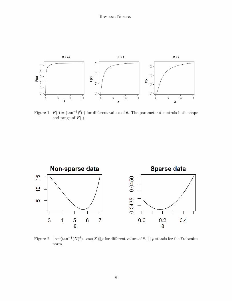
Thus by modifying the edge potential function in this way using a bounded function ofX, we can allow unrestricted support for all the parameters, allowing one to estimate bothpositive and negative dependence. Under the monotonicity restrictions on F (·), inference onthe conditional independence structure tends to be robust to the specific form chosen. We letF (·) = (tan−1(·))θ for some positive θ ∈ R+ to define a flexible class of monotone increasingbounded functions. The exponent θ provides additional flexibility, including impactingthe range of F (X),

(0, (π2 )θ

). The parameter θ can be estimated along with the other

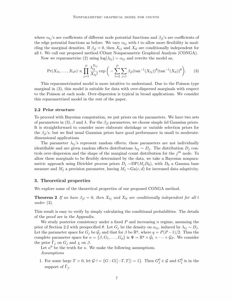
parameters, including the baseline parameters α controlling the marginal count distributionsand the coefficients βjl controlling the graphical dependence structure. For simplicity andinterpretability, we propose to estimate θ to minimize the difference in covariance betweenF (X) and X. Figure 1 illustrates how θ controls the range and shape of F (·). Figure 2shows how the difference between covariances of F (X) and X vary for different values ofθ in sparse and non-sparse data cases. In both cases, the difference function has a uniqueminimizer. Although the same strategy could be used to tune the truncation parameterin the Yang et al. (2013) approach, issues arise in estimating the support of the data basedon a finite sample, as new data may fall outside of the estimated support. Besides, theirapproach is less flexible in relying on parametric assumptions, while we use a mixture modelfor the αs to induce a nonparametric structure.

Letting Xt denote the tth independent realization of X, for t = 1, . . . , n, the pmf is

Pr(Xt1, . . . , XtP ) ∝ exp

( P∑j=1

[αtjXtj − log(Xtj !)]−

P∑l=2

∑j<l

βjl(tan−1(Xtj))θ(tan−1(Xtl))

θ

), (2)

5

Roy and Dunson

Figure 1: F (·) = (tan−1)θ(·) for different values of θ. The parameter θ controls both shapeand range of F (·).

Figure 2: ‖cov(tan−1(X)θ)−cov(X)‖F for different values of θ. ‖‖F stands for the Frobeniusnorm.

6


where αtj ’s are coefficients of different node potential functions and βjl’s are coefficients ofthe edge potential functions as before. We vary αtj with t to allow more flexibility in mod-eling the marginal densities. If βjl = 0, then Xtj and Xtl are conditionally independent forall t. We call our proposed method COunt Nonparametric Graphical Analysis (CONGA).

Now we reparametrize (2) using log(λtj) = αtj and rewrite the model as,

Pr(Xt1, . . . , XtP ) ∝P∏j=1

λXtj

tj

Xtj !exp

(−

P∑l=2

∑j<l

βjl(tan−1(Xtj))θ(tan−1(Xtl))

θ

). (3)

This reparametrizated model is more intuitive to understand. Due to the Poisson typemarginal in (3), this model is suitable for data with over-dispersed marginals with respectto the Poisson at each node. Over-dispersion is typical in broad applications. We considerthis reparametrized model in the rest of the paper.

2.2 Prior structure

To proceed with Bayesian computation, we put priors on the parameters. We have two setsof parameters in (3), β and λ. For the βjl parameters, we choose simple iid Gaussian priors.It is straightforward to consider more elaborate shrinkage or variable selection priors forthe βjl’s, but we find usual Gaussian priors have good performance in small to moderate-dimensional applications

The parameter λtj ’s represent random effects; these parameters are not individuallyidentifiable and are given random effects distributions λtj ∼ Dj . The distribution Dj con-trols over-dispersion and the shape of the marginal count distribution for the jth node. Toallow these marginals to be flexibly determined by the data, we take a Bayesian nonpara-metric approach using Dirichlet process priors Dj ∼DP(MjD0), with D0 a Gamma basemeasure and Mj a precision parameter, having Mj ∼Ga(c, d) for increased data adaptivity.

3. Theoretical properties

We explore some of the theoretical properties of our proposed CONGA method.

Theorem 2 If we have βjl = 0, then Xtj and Xtl are conditionally independent for all tunder (3).

This result is easy to verify by simply calculating the conditional probabilities. The detailsof the proof are in the Appendix.

We study posterior consistency under a fixed P and increasing n regime, assuming theprior of Section 2.2 with prespecified θ. Let Gj be the density on αtj , induced by λtj ∼ Dj .Let the parameter space for Gj be Gj and that for β be Rq, where q = P (P −1)/2. Thus thecomplete parameter space for κ = β,G1, . . . , Gp is Ψ = Rq × G1 × · · · × GP . We considerthe prior Γj on Gj and χ on β.

Let κ0 be the truth for κ. We make the following assumptions.Assumptions

1. For some large T > 0, let Ga = G : G([−T, T ]) = 1. Then G0j ∈ G and G0

j is in the

support of Γj .

7

Roy and Dunson

2. For some large C > 0, let Q = β : ‖β‖∞ < C, where ‖ · ‖∞ stands for the infinitynorm. Then β0 ∈ Q and β0 is in the support of χ.

3. E(Xtj) <∞ for all pairs of (t, j)

Theorem 3 Under the assumptions, 1-3, the posterior for κ is consistent at κ0.

We show that the truth belongs to the Kullback-Leibler support of the prior. Thus the

posterior probability of any neighborhood around the true p.m.f converges to one in P(n)κ0 -

probability as n goes to∞ as a consequence of Schwartz (1965). Here P(n)κ is the distribution

of a sample of n observations with parameter κ. Hence, the posterior is weakly consistent.The posterior is said to be strongly consistent if the posterior probability of any neighbor-hood around the true p.m.f convergences to one almost-surely. Support of the data is acountable space. The weak and strong topologies on countable spaces are equivalent byScheffe’s theorem. In particular, weak topology and total variation topology are equivalentfor discrete data. Weak consistency implies strong consistency. Thus the posterior for κ isalso strongly consistent at κ0. A detailed proof is in the Appendix.

Instead of assuming bounded support on the true distribution of random effects, onecan also assume it to have sub-Gaussian tails. The posterior consistency result still holdswith minor modifications in the current proof. Establishing graph selection consistency ofthe proposed method is an interesting area of future research when p is growing with n andλtj ’s are fixed effects. Since we are interested in a non-parametric graphical model, we donot explore that in this paper.

4. Computation

As motivated in Section 2.1, we estimate θ to minimize the differences in the sample covari-ance of X and F (X). In particular, the criteria is to minimize ‖cov(tan−1(X)θ)−cov(X)‖F .This is a simple one dimensional optimization problem, which is easily solved numerically.

To update the other parameters, we use an MCMC algorithm, building on the approachof Roy et al. (2018). We generate proposals for Metropolis-Hastings (MH) using a Gibbssampler derived under an approximated model. To avoid calculation of the global normal-izing constant in the complete likelihood, we consider a pseudo-likelihood correspondingto a product of conditional likelihoods at each node. This requires calculations of P localnormalizing constants which is computationally tractable.

The conditional likelihood at the j-th node is,

P (Xtj |Xt,−j) =

exp[log(λtj)Xtj − log(Xtj !) −

∑j 6=l βjltan−1(Xtj)θtan−1(Xtl)θ

]∑∞Xtj=0 exp

[log(λtj)Xtj − log(Xtj !) −

∑j 6=l βjltan−1(Xtj)θtan−1(Xtl)θ

] (4)

The normalizing constant is

∞∑Xtj=0

exp[log(λtj)Xtj − log(Xtj !) −

∑j 6=l

βjltan−1(Xtj)θtan−1(Xtl)θ].

8


We truncate this sum at a sufficiently large value B for the purpose of evaluating theconditional likelihood. The error in this approximation can be bounded by

exp(λtj)(1− CP (B + 1, λtj)) exp

−

∑j 6=l:βjl<0

βjl(π/2)θ(tan−1(Xtl))θ

,

where CP (x, l) is the cumulative distribution function of the Poisson distribution withmean l evaluated at x. The above bound can in turn be bounded by a similar expressionwith (tan−1(Xtl))

θ replaced by (π/2)θ. One can tune B based on the resulting bound onthe approximation error. In our simulation setting, even B = 70 makes the above boundnumerically zero. We use B = 100 as a default choice for all of our computations.

We update λ.j using the MCMC sampling scheme described in Chapter 5 of Ghosaland Van der Vaart (2017) for the Dirichlet process mixture prior of λij based on the aboveconditional likelihood. For clarity this algorithm is described below:

(i) Calculate the probability vector Qj for each j such that Qj(k) = Pois(Xij , λkj) andQj(i) = MjGa(λi,j , a+Xi,j , b+ 1).

(ii) Sample an index l from 1 : T with probability Qj/∑

kQj(k).

(iii) If l 6= i, λij = λlj . Otherwise sample a new value as described below.

(iv) Mj is sampled from Gamma(c + U, d − log(δ)), where U is the number of uniqueelements in λ.j , δ is sampled from Beta(Mj , T ), and Mj ∼Ga(c, d) a priori.

When we have to generate a new value for λtj in step (iii), we consider the followingscheme.

(i) Generate a candidate λctj from Gamma(a+Xtj , b+ 1).

(ii) Adjust the update λctj = λ0tj +K1(λctj−λ0

tj), where λ0tj is the current value and K1 < 1

is a tuning parameter, adjusted with respect to the acceptance rate of the resultingMetropolis-Hastings (MH) step.

(iii) We use the pseudo-likelihood based on the conditional likelihoods in (4) to calculatethe MH acceptance probability.

To generate β, we consider a new likelihood that the standardized (tan−1(Xtl))θ follows

a multivariate Gaussian distribution with precision matrix Ω such that Ωpq = Ωqp = βpqwith p < q and Ωpp = (V ar((tan−1(Xtl))

θ)−1)pp. Thus diagonal entries do not changeover iterations. We update Ωl,−l = Ωl,i : i 6= l successively. We also define Ω−l,−l as thesubmatrix by removing l-th row and column. Let s = (F (x)− F (X))T (F (x)− F (X)). Thuss is the P × P gram matrix of (tan−1X)θ, standardized over columns.

(i) Generate an update for Ωl,−l using the posterior distribution as in Wang (2012). Thusa candidate Ωc

l,−l is generated from MVN(−Csl,−l, C), where C = ((s22 + γ)Ω−1−l,−l +

D−1l )−1, where Dl is the prior variance corresponding to Ωl,−l

9

Roy and Dunson

(ii) Adjust the update Ωcl,−l = Ω0

l,−l + K2(Ωc

l,−l−Ω0l,−l)

‖(Ωcl,−l−Ω0

l,−l)‖2, where Ω0

l,−l is the current value

and K2 is a tuning parameter, adjusted with respect to the acceptance rate of thefollowing MH step. Also K2 should always be less than ‖(Ωc

l,−l − Ω0l,−l)‖2.

(iii) Use the pseudo-likelihood based on the conditional likelihoods in (4), multiplying overt to calculate the MH acceptance probability. π(θ0|θc) = π(θG) and π(θc|θ0) = π(θ′G),where θG is the original Gibbs update.

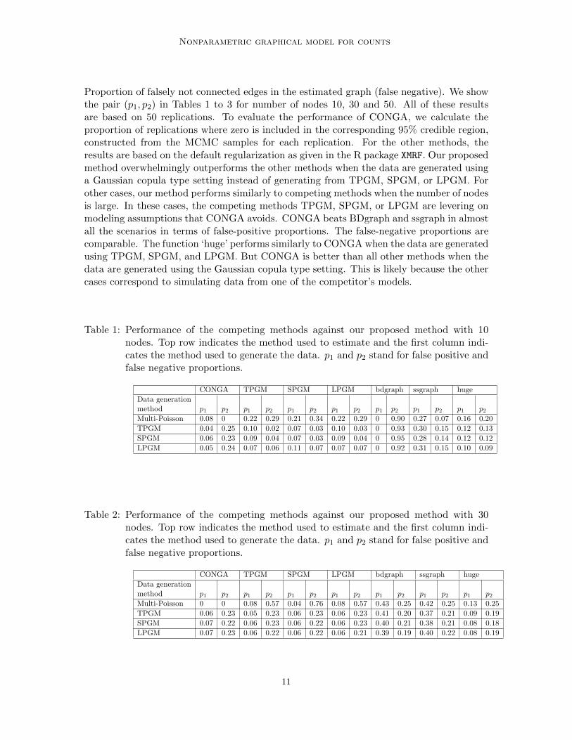
5. Simulation

We consider four different techniques for generating multivariate count data. One approachis based on a Gaussian copula type setting. The other three are based on competingmethods. We compare the methods based on false positive and false negative proportions.We include an edge in the graph between the jth and lth nodes if the 95% credible intervalfor βjl does not include zero. There is a decision-theoretic proof to justify such an approachin Thulin (2014). We compare our method CONGA with TPGM, SPGM, LPGM, huge,BDgraph, and ssgraph. The first three are available in R package XMRF and the last two arein R packages BDgraph and ssgraph respectively. The function huge is from R package hugewhich fits a nonparanormal graphical model. The last two methods fit graphical modelsusing Gaussian copulas and ssgraph uses spike and slab priors in estimating the edges.

To simulate data under the first scheme, we follow the steps given below.

(i) Generate n many multivariate normals of length c from MVN(0c,Ω−1c×c), where 0c is

the vector of zeros of length c. This produces a matrix X of dimension n× c.

(ii) We calculate the matrix Pn×c, which is Pij = Φ(Xij), where Φ is the cumulativedensity function of the standard normal.

(iii) The Poisson random variable Yn×c is Yij = QP (Pij , λ) for a given mean parameter λwith QP the quantile function of Poisson(λ).

Let X:,l denote the l-th column of X. In the above data generation setup, Ωpq = 0implies that Y:,p and Y:,q are conditionally independent due to Lemma 3 of Liu et al. (2009).The marginals are allowed to be multimodal at some of the nodes, which is not possibleunder the other simulation schemes.

Apart from the above approach, we also generate the data using R package XMRF from themodels Sub-Linear Poisson Graphical Model (SPGM), Truncated Poisson graphical Model(TPGM) (Yang et al., 2013), and Local Poisson Graphical Model (LPGM) (Allen and Liu,2012).

We choose ν3 = 100, which is the prior variance of the normal prior of βjl for all j, l.The choice ν3 = 100 makes the prior weakly informative. The parameter γ is chosen to be5 as given in Wang (2012). For the gamma distribution, we consider a = b = 1. For theDirichlet process mixture, we take c = d = 10. We consider n = 100 and P = 10, 30, 50.We collect 5000 post burn MCMC samples after burning in 5000 MCMC samples.

We compare the methods based on two quantities p1 and p2. We define these as p1

= Proportion of falsely connected edges in the estimated graph (false positive) and p2 =

10


Proportion of falsely not connected edges in the estimated graph (false negative). We showthe pair (p1, p2) in Tables 1 to 3 for number of nodes 10, 30 and 50. All of these resultsare based on 50 replications. To evaluate the performance of CONGA, we calculate theproportion of replications where zero is included in the corresponding 95% credible region,constructed from the MCMC samples for each replication. For the other methods, theresults are based on the default regularization as given in the R package XMRF. Our proposedmethod overwhelmingly outperforms the other methods when the data are generated usinga Gaussian copula type setting instead of generating from TPGM, SPGM, or LPGM. Forother cases, our method performs similarly to competing methods when the number of nodesis large. In these cases, the competing methods TPGM, SPGM, or LPGM are levering onmodeling assumptions that CONGA avoids. CONGA beats BDgraph and ssgraph in almostall the scenarios in terms of false-positive proportions. The false-negative proportions arecomparable. The function ‘huge’ performs similarly to CONGA when the data are generatedusing TPGM, SPGM, and LPGM. But CONGA is better than all other methods when thedata are generated using the Gaussian copula type setting. This is likely because the othercases correspond to simulating data from one of the competitor’s models.

Table 1: Performance of the competing methods against our proposed method with 10nodes. Top row indicates the method used to estimate and the first column indi-cates the method used to generate the data. p1 and p2 stand for false positive andfalse negative proportions.

CONGA TPGM SPGM LPGM bdgraph ssgraph huge

Data generationmethod p1 p2 p1 p2 p1 p2 p1 p2 p1 p2 p1 p2 p1 p2

Multi-Poisson 0.08 0 0.22 0.29 0.21 0.34 0.22 0.29 0 0.90 0.27 0.07 0.16 0.20

TPGM 0.04 0.25 0.10 0.02 0.07 0.03 0.10 0.03 0 0.93 0.30 0.15 0.12 0.13

SPGM 0.06 0.23 0.09 0.04 0.07 0.03 0.09 0.04 0 0.95 0.28 0.14 0.12 0.12

LPGM 0.05 0.24 0.07 0.06 0.11 0.07 0.07 0.07 0 0.92 0.31 0.15 0.10 0.09




Multi-Poisson 0 0 0.08 0.57 0.04 0.76 0.08 0.57 0.43 0.25 0.42 0.25 0.13 0.25

TPGM 0.06 0.23 0.05 0.23 0.06 0.23 0.06 0.23 0.41 0.20 0.37 0.21 0.09 0.19

SPGM 0.07 0.22 0.06 0.23 0.06 0.22 0.06 0.23 0.40 0.21 0.38 0.21 0.08 0.18

LPGM 0.07 0.23 0.06 0.22 0.06 0.22 0.06 0.21 0.39 0.19 0.40 0.22 0.08 0.19

11

Roy and Dunson




Multi-Poisson 0 0 0.01 0.88 0.02 0.76 0.02 0.75 0.46 0.22 0.44 0.25 0.15 0.26

TPGM 0.11 0.23 0.03 0.29 0.03 0.33 0.03 0.33 0.42 0.23 0.43 0.25 0.07 0.21

SPGM 0.11 0.25 0.03 0.33 0.03 0.31 0.03 0.33 0.43 0.21 0.41 0.26 0.08 0.22

LPGM 0.12 0.23 0.03 0.32 0.03 0.34 0.03 0.31 0.43 0.23 0.44 0.26 0.08 0.21

6. Neuron spike count application

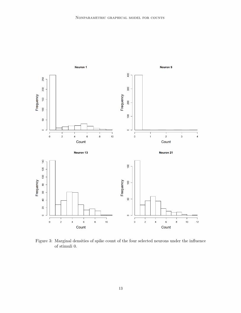
The dataset records neuron spike counts in mice across 37 neurons in the brain under theinfluence of three different external stimuli, 2-D sinusoids with vertical gradient, horizontalgradient, and the sum. These neurons are from the same depth of the visual cortex of amouse. The data are collected for around 400-time points. In Figure 3, we plot the marginaldensities of the spike counts of four neurons under the influence of stimuli 0. We see thatthere are many variations in the marginal densities, and the densities are multi-modal forsome of the cases. Marginally at each node, we also have that the variance is more thanthe corresponding mean for each of the three stimuli.

6.1 Estimation

We apply exactly the same computational approach as used in the simulation studies. Toadditionally obtain a summary of the weight of evidence of an edge between nodes j andl, we calculate Sjl =

(|0.5 − P (βjl > 0)|

)/0.5, with P (βjl > 0) the posterior probability

estimated from the MCMC samples. We plot the estimated graph with edge thicknessproportional to the values of Sjl. Thus thicker edges suggest greater evidence of an edge inFigures 4 to 6. To test for similarity in the graph across stimuli, we estimate 95% credible

regions for ∆s,s′

jl = βsjl − βs′jl , denoting the difference in the (j, l) edge weight parameter

under stimuli s and s′, respectively. We flag those edges (j, l) having 95% credible intervals

for ∆s,s′

jl not including zero as significantly different across stimuli.

6.2 Inference

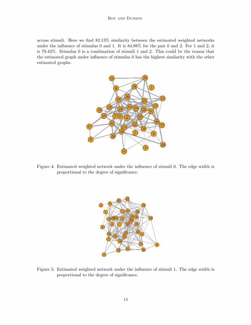
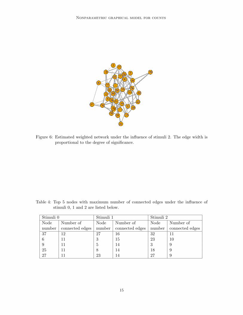
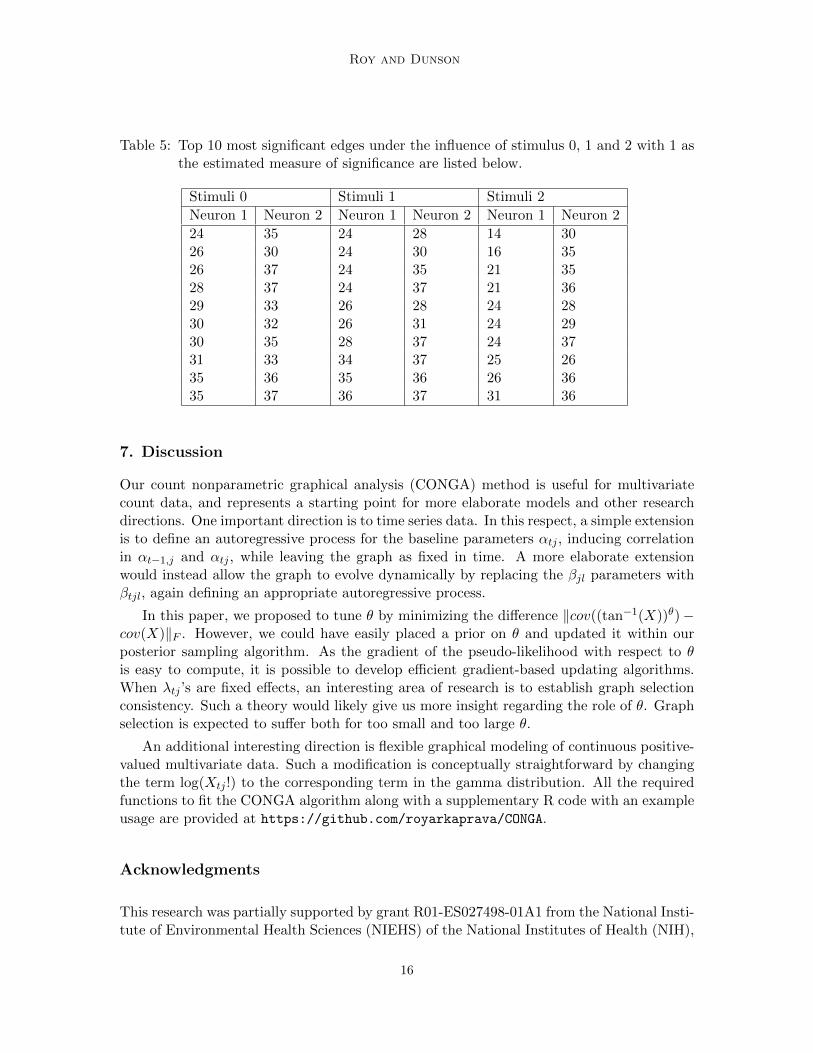
We find that there are 129, 199, and 110 connected edges respectively for stimuli 0, 1, and2. Among these edges, 38 are common for stimulus 0 and 1. The number is 15 for stimulus0 and 2, and 28 for stimulus 1 and 2. There are 6 edges that are common for all of thestimuli. These are (13,16), (8,27), (5,8), (33,35), (3,4) and (9, 14). Each node has at leastone edge with another node. We plot the estimated network in Figures 4 to 6. We calculatethe number of connected edges for each node and list the 5 most connected nodes in Table 4.We also list the most significant 10 edges for each stimulus in Table 5. We find that node27 is present in all of them. This node seems to have significant interconnections with othernodes for all of the stimuli. We also test the similarity in the estimated weighted network

12


Figure 3: Marginal densities of spike count of the four selected neurons under the influenceof stimuli 0.

13

Roy and Dunson

across stimuli. Here we find 82.13% similarity between the estimated weighted networksunder the influence of stimulus 0 and 1. It is 84.98% for the pair 0 and 2. For 1 and 2, itis 79.43%. Stimulus 0 is a combination of stimuli 1 and 2. This could be the reason thatthe estimated graph under influence of stimulus 0 has the highest similarity with the otherestimated graphs.

Figure 4: Estimated weighted network under the influence of stimuli 0. The edge width isproportional to the degree of significance.


14



Table 4: Top 5 nodes with maximum number of connected edges under the influence ofstimuli 0, 1 and 2 are listed below.

Stimuli 0 Stimuli 1 Stimuli 2

Node Number of Node Number of Node Number ofnumber connected edges number connected edges number connected edges

37 12 27 16 32 116 11 3 15 23 109 11 5 14 3 925 11 8 14 18 927 11 23 14 27 9

15

Roy and Dunson

Table 5: Top 10 most significant edges under the influence of stimulus 0, 1 and 2 with 1 asthe estimated measure of significance are listed below.

Stimuli 0 Stimuli 1 Stimuli 2

Neuron 1 Neuron 2 Neuron 1 Neuron 2 Neuron 1 Neuron 2

24 35 24 28 14 3026 30 24 30 16 3526 37 24 35 21 3528 37 24 37 21 3629 33 26 28 24 2830 32 26 31 24 2930 35 28 37 24 3731 33 34 37 25 2635 36 35 36 26 3635 37 36 37 31 36

7. Discussion

Our count nonparametric graphical analysis (CONGA) method is useful for multivariatecount data, and represents a starting point for more elaborate models and other researchdirections. One important direction is to time series data. In this respect, a simple extensionis to define an autoregressive process for the baseline parameters αtj , inducing correlationin αt−1,j and αtj , while leaving the graph as fixed in time. A more elaborate extensionwould instead allow the graph to evolve dynamically by replacing the βjl parameters withβtjl, again defining an appropriate autoregressive process.

In this paper, we proposed to tune θ by minimizing the difference ‖cov((tan−1(X))θ)−cov(X)‖F . However, we could have easily placed a prior on θ and updated it within ourposterior sampling algorithm. As the gradient of the pseudo-likelihood with respect to θis easy to compute, it is possible to develop efficient gradient-based updating algorithms.When λtj ’s are fixed effects, an interesting area of research is to establish graph selectionconsistency. Such a theory would likely give us more insight regarding the role of θ. Graphselection is expected to suffer both for too small and too large θ.

An additional interesting direction is flexible graphical modeling of continuous positive-valued multivariate data. Such a modification is conceptually straightforward by changingthe term log(Xtj !) to the corresponding term in the gamma distribution. All the requiredfunctions to fit the CONGA algorithm along with a supplementary R code with an exampleusage are provided at https://github.com/royarkaprava/CONGA.

Acknowledgments

This research was partially supported by grant R01-ES027498-01A1 from the National Insti-tute of Environmental Health Sciences (NIEHS) of the National Institutes of Health (NIH),

16

https://github.com/royarkaprava/CONGA


grant R01-MH118927 from the National Institute of Mental Health (NIMH) of the NIH, andgrant R01ES028804-01 from National Institute of Environmental Health Sciences (NIEHS).

17

Roy and Dunson

Appendix

Proof of Theorem 2

The conditional probability is given by,

P (Xtj , Xtl|Xt,−(j,l)) =

exp(∑

h∈(j,l)(αthXth − log(Xth!)−∑

g 6=h βgh(tan−1(Xtg))θ(tan−1(Xth))θ

)∑∞Xtj=0

∑∞Xtl=0 exp

(∑h∈(j,l)(αthXth − log(Xth!)−

∑g 6=h βgh(tan−1(Xtg))θ(tan−1(Xth))θ

) ,where Xt,−(j,l) = Xti : i 6= (j, l) and log(λth) = αth. Since βjl = 0, we can breakthe exponentiated terms into two such that Xtj and Xjl are separated out. That wouldimmediately give us, P (Xtj , Xtl|Xt,−(j,l)) = P (Xtj |Xt,−(j,l))P (Xtl|Xt,−(j,l)).

Proof of Theorem 3

For q, q∗ ∈ the space of probability measure P, let the Kullback-Leibler divergences be givenby

K(q∗, q) =

∫q∗ log

q∗

qV (q∗, q) =

∫q∗ log2 q

∗

q.

Let us denote pi,α,β(Xi) as the probability distribution of the data given below,

1

A(αi, β)exp

( P∑j=1

[αijXij − log(Xij !)] +P∑l=2

∑j<l

βijl(tan−1(Xij))θ(tan−1(Xil))

θ

),

where A(αi, β) is the normalizing constant and αi = αi1, . . . , αiP , β = βjl : 1 ≤ j < l ≤P. Let E(Xij) = Q. We have,

∂ log(A(αi, β))

∂αij=A(αij , β)

A(αi, β))E(Xij) ≤ Q, as,

A(αij , β)

A(αi, β))≤ 1,

and

∂(A(αi, β))

∂βjl≤ (

π

2)2θ(A(αi, β))

Thus we have, ∂ log(A(αi,β))∂αik

≤ Q for all 1 ≤ k ≤ P and ∂ log(A(αi,β))∂βjl

≤ (π2 )2θ.

This implies,

−P∑j=1

vij ≤ logpi,κ0(Xi)

pi,κ(Xi)≤

P∑j=1

vij ,

where vtj = (TQXtj + C∑P

l=2

∑j<l(tan−1(Xtj)) + (π2 )2θ(T + qC). We have E(vtj) < ∞

due to the last assumption. From the dominated convergence theorem as n→∞, we haveκ converges to κ0. Thus Kullback-Leibler divergences go to zero.

Thus the posterior is weakly consistent. The weak and strong topologies on count-able spaces are equivalent by Scheffe’s theorem. Thus the posterior for κ is also stronglyconsistent at κ0.

18


References

John Aitchison and CH Ho. The multivariate Poisson-log normal distribution. Biometrika,76(4):643–653, 1989.

Genevera I Allen and Zhandong Liu. A log-linear graphical model for inferring geneticnetworks from high-throughput sequencing data. In Bioinformatics and Biomedicine(BIBM), 2012 IEEE International Conference on, pages 1–6. IEEE, 2012.

Adrian Baddeley and Rolf Turner. Practical maximum pseudolikelihood for spatial pointpatterns: (with discussion). Australian & New Zealand Journal of Statistics, 42(3):283–322, 2000.

Onureena Banerjee, Laurent El Ghaoui, and Alexandre d’Aspremont. Model selectionthrough sparse maximum likelihood estimation for multivariate aussian or binary data.Journal of Machine Learning Research, 9(Mar):485–516, 2008.

Julian Besag. Spatial interaction and the statistical analysis of lattice systems. Journal ofthe Royal Statistical Society. Series B (Methodological), pages 192–236, 1974.

Julian Besag. Statistical analysis of non-lattice data. The Statistician, pages 179–195, 1975.

KS Chan and Johannes Ledolter. Monte carlo em estimation for time series models involvingcounts. Journal of the American Statistical Association, 90(429):242–252, 1995.

Shizhe Chen, Daniela M Witten, and Ali Shojaie. Selection and estimation for mixedgraphical models. Biometrika, 102(1):47–64, 2014.

Siddhartha Chib and Rainer Winkelmann. Markov chain monte carlo analysis of correlatedcount data. Journal of Business & Economic Statistics, 19(4):428–435, 2001.

Julien Chiquet, Mahendra Mariadassou, and Stephane Robin. Variational inference forsparse network reconstruction from count data. arXiv preprint arXiv:1806.03120, 2018.

Francis Comets. On consistency of a class of estimators for exponential families of Markovrandom fields on the lattice. The Annals of Statistics, pages 455–468, 1992.

Victor De Oliveira. Bayesian analysis of conditional autoregressive models. Annals of theInstitute of Statistical Mathematics, 64(1):107–133, 2012.

Victor De Oliveira. Hierarchical Poisson models for spatial count data. Journal of Multi-variate Analysis, 122:393–408, 2013.

Peter J Diggle, JA Tawn, and RA Moyeed. Model-based geostatistics. Journal of the RoyalStatistical Society: Series C (Applied Statistics), 47(3):299–350, 1998.

Adrian Dobra and Alex Lenkoski. Copula Gaussian graphical models and their applicationto modeling functional disability data. The Annals of Applied Statistics, 5(2A):969–993,2011.

19

Roy and Dunson

Adrian Dobra, Alex Lenkoski, and Abel Rodriguez. Bayesian inference for general Gaussiangraphical models with application to multivariate lattice data. Journal of the AmericanStatistical Association, 106(496):1418–1433, 2011.

Adrian Dobra, Reza Mohammadi, et al. Loglinear model selection and human mobility.The Annals of Applied Statistics, 12(2):815–845, 2018.

Alan E Gelfand and Penelope Vounatsou. Proper multivariate conditional autoregressivemodels for spatial data analysis. Biostatistics, 4(1):11–15, 2003.

Subhashis Ghosal and Aad Van der Vaart. Fundamentals of nonparametric Bayesian infer-ence, volume 44. Cambridge University Press, 2017.

Fabian Hadiji, Alejandro Molina, Sriraam Natarajan, and Kristian Kersting. Poisson depen-dency networks: Gradient boosted models for multivariate count data. Machine Learning,100(2-3):477–507, 2015.

John M Hammersley and Peter Clifford. Markov fields on finite graphs and lattices. Un-published manuscript, 1971.

John L Hay and Anthony N Pettitt. Bayesian analysis of a time series of counts withcovariates: an application to the control of an infectious disease. Biostatistics, 2(4):433–444, 2001.

David Inouye, Pradeep Ravikumar, and Inderjit Dhillon. Admixture of Poisson mrfs: Atopic model with word dependencies. In International Conference on Machine Learning,pages 683–691, 2014.

David I Inouye, Pradeep Ravikumar, and Inderjit S Dhillon. Generalized root models:beyond pairwise graphical models for univariate exponential families. arXiv preprintarXiv:1606.00813, 2016a.

David I Inouye, Pradeep Ravikumar, and Inderjit S Dhillon. Square root graphical mod-els: Multivariate generalizations of univariate exponential families that permit positivedependencies. arXiv preprint arXiv:1603.03629, 2016b.

David I Inouye, Eunho Yang, Genevera I Allen, and Pradeep Ravikumar. A review ofmultivariate distributions for count data derived from the Poisson distribution. WileyInterdisciplinary Reviews: Computational Statistics, 9(3):e1398, 2017.

Ali Jalali, Pradeep Ravikumar, Vishvas Vasuki, and Sujay Sanghavi. On learning discretegraphical models using group-sparse regularization. In Proceedings of the FourteenthInternational Conference on Artificial Intelligence and Statistics, pages 378–387, 2011.

Jens Ledet Jensen and Hans R Kunsch. On asymptotic normality of pseudo likelihoodestimates for pairwise interaction processes. Annals of the Institute of Statistical Mathe-matics, 46(3):475–486, 1994.

Mladen Kolar and Eric P Xing. Improved estimation of high-dimensional Ising models.arXiv preprint arXiv:0811.1239, 2008.

20


Mladen Kolar, Le Song, Amr Ahmed, Eric P Xing, et al. Estimating time-varying networks.The Annals of Applied Statistics, 4(1):94–123, 2010.

Han Liu, John Lafferty, and Larry Wasserman. The nonparanormal: Semiparametric esti-mation of high dimensional undirected graphs. Journal of Machine Learning Research,10(Oct):2295–2328, 2009.

Shigeru Mase. Marked gibbs processes and asymptotic normality of maximum pseudo-likelihood estimators. Mathematische Nachrichten, 209(1):151–169, 2000.

Abdolreza Mohammadi, Ernst C Wit, et al. Bayesian structure learning in sparse Gaussiangraphical models. Bayesian Analysis, 10(1):109–138, 2015.

Abdolreza Mohammadi, Fentaw Abegaz, Edwin van den Heuvel, and Ernst C Wit. Bayesianmodelling of dupuytren disease by using Gaussian copula graphical models. Journal ofthe Royal Statistical Society: Series C (Applied Statistics), 66(3):629–645, 2017.

Jared S Murray, David B Dunson, Lawrence Carin, and Joseph E Lucas. Bayesian Gaussiancopula factor models for mixed data. Journal of the American Statistical Association,108(502):656–665, 2013.

Johan Pensar, Henrik Nyman, Juha Niiranen, Jukka Corander, et al. Marginal pseudo-likelihood learning of discrete Markov network structures. Bayesian analysis, 12(4):1195–1215, 2017.

Pradeep Ravikumar, Martin J Wainwright, and John D Lafferty. High-dimensional Isingmodel selection using `1-regularized logistic regression. The Annals of Statistics, 38(3):1287–1319, 2010.

Arkaprava Roy, Brian J Reich, Joseph Guinness, Russell T Shinohara, and Ana-MariaStaicu. Spatial shrinkage via the product independent Gaussian process prior. arXivpreprint arXiv:1805.03240, 2018.

Lorraine Schwartz. On bayes procedures. Zeitschrift fur Wahrscheinlichkeitstheorie undverwandte Gebiete, 4(1):10–26, 1965.

Mans Thulin. Decision-theoretic justifications for Bayesian hypothesis testing using crediblesets. Journal of Statistical Planning and Inference, 146:133–138, 2014.

Marijtje AJ Van Duijn, Krista J Gile, and Mark S Handcock. A framework for the compar-ison of maximum pseudo-likelihood and maximum likelihood estimation of exponentialfamily random graph models. Social Networks, 31(1):52–62, 2009.

Martin J Wainwright, John D Lafferty, and Pradeep K Ravikumar. High-dimensional graph-ical model selection using `1 regularized logistic regression. In Advances in neural infor-mation processing systems, pages 1465–1472, 2007.

Hao Wang. Bayesian graphical lasso models and efficient posterior computation. BayesianAnalysis, 7(4):867–886, 2012.

21

Roy and Dunson

Hao Wang. Scaling it up: Stochastic search structure learning in graphical models. BayesianAnalysis, 10(2):351–377, 2015.

Yiyi Wang and Kara M Kockelman. A Poisson-lognormal conditional-autoregressive modelfor multivariate spatial analysis of pedestrian crash counts across neighborhoods. AccidentAnalysis & Prevention, 60:71–84, 2013.

Michel Wedel, Ulf Bockenholt, and Wagner A Kamakura. Factor models for multivariatecount data. Journal of Multivariate Analysis, 87(2):356–369, 2003.

Peter Xue-Kun Song. Multivariate dispersion models generated from Gaussian copula.Scandinavian Journal of Statistics, 27(2):305–320, 2000.

Eunho Yang, Pradeep K Ravikumar, Genevera I Allen, and Zhandong Liu. On Poissongraphical models. In Advances in Neural Information Processing Systems, pages 1718–1726, 2013.

Eunho Yang, Pradeep Ravikumar, Genevera I Allen, and Zhandong Liu. Graphical mod-els via univariate exponential family distributions. The Journal of Machine LearningResearch, 16(1):3813–3847, 2015.

Mingyuan Zhou, Lauren A Hannah, David B Dunson, and Lawrence Carin. Beta-negativebinomial process and Poisson factor analysis. In AISTATS, pages 1462–1471, 2012.

Xiang Zhou and Scott C Schmidler. Bayesian parameter estimation in Ising and Pottsmodels: A comparative study with applications to protein modeling. Technical report,Duke University, 2009.

22

Documents

Nonparametric graphical model for counts