Statistics & Probability Letters 8 (1989) 179-184

North-Holland

June 1989

NONPARAMETRIC BAYESIAN ANALYSIS OF THE ACCELERATED FAILURE TIME MODEL

Wesley JOHNSON

Division of Statistics, University of California, Davis, CA 95616, USA

Ronald CHRISTENSEN

Department of Mathematical Sciences, Montana State University, Bozeman, MT 59717, USA

Received April 1988 Revised July 1988

Abstract: The baseline probability distribution for accelerated failure time is modeled with a Dir&let process. A fully Bayesian analysis is developed for the estimation of regression coefficients as well as for the estimation of survival curves. The

practical difficulties associated with this theoretically desirable analysis are emphasized.

Keywords: accelerated failure time, Dirichlet process, empirical Bayes, non-parametric Bayes, semi-parametric model.

1. Introduction

The role of covariates in Bayesian nonparametric reliability analysis has received little attention. Kalbfleisch (1978) and Christensen and Johnson (1988) have developed partially Bayesian analyses for the Cox model and for the accelerated failure time model respectively. Both deal with the possibility of right censored observations. Kalbfleisch examined Gamma process priors and mentioned the use of Dirichlet priors. Christensen and Johnson considered only Dirichlet process priors. Burridge (1981) extended Kalbfleisch’s results for the Cox model by examining grouped data and arbitrary independent increments process priors. Burridge illustrated his results using Gamma processes. A fully Bayesian approach to these models has not yet been presented. In what follows, we examine the fully Bayesian analysis of the accelerated failure time model with uncensored data. The censored data problem is considerably more difficult.

In the accelerated failure time model, failure times T = (T,, . . . , Tn)T are modeled as

T = e-XTpV I

where xi=(xil,...,xip) T is a known vector of covariates, p is an unknown vector of regression coefficients and V = (V,, . . . , Vn)T is a random sample from a baseline distribution P. For our Bayesian analysis, we assume independent prior distributions on /3 and P. In particular, we take the prior on P to be a Dirichlet process with parametric measure a( .) defined on [0, 00). Section 2 discusses the fully Bayesian solution. Section 3 contains some concluding remarks.

2. Fully Bayesian approach

We use notation similar to Antoniak (1974). P is from a Dirichlet process with parameter (Y, written

p -S(a),

0167-7152/89/$3.50 0 1989, Elsevier Science Publishers B.V. (North-Holland) 179

Volume 8. Number 2 STATISTICS & PROBABILITY LETTERS June 1989

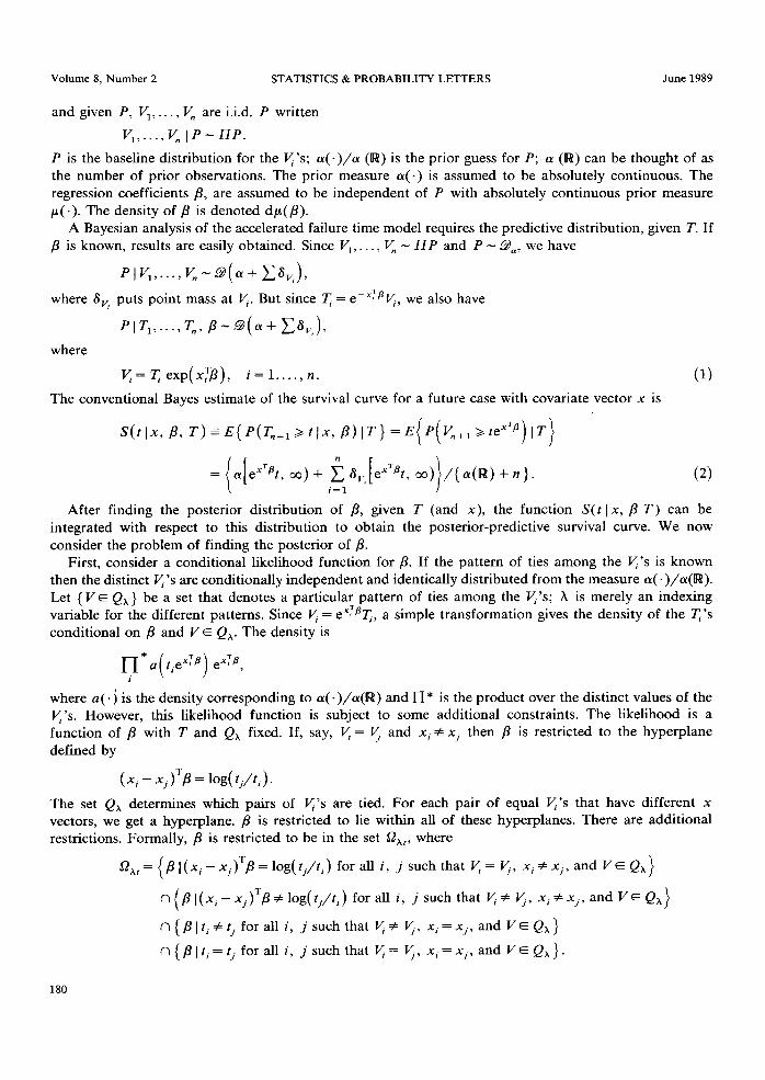
and given P, V ,,__. , V, are Cd. P written

V I,“‘, v, IP-rIP.

P is the baseline distribution for the V’s; (u( .)/a (R) is the prior guess for P; a (R) can be thought of as the number of prior observations. The prior measure CX( .) is assumed to be absolutely continuous. The regression coefficients /3, are assumed to be independent of P with absolutely continuous prior measure p( .). The density of p is denoted dp(p).

A Bayesian analysis of the accelerated failure time model requires the predictive distribution, given T. If /3 is known, results are easily obtained. Since VI,. . . , V, - IIP and P - ga, we have

PlVi:,..., K-++ D,)?

where 6, puts point mass at V. But since q = eCxfsV, we also have

PIT,,..., T,> P-+x+C&,),

where

V=q.exp(xTp), i=l,..., n. (1) The conventional Bayes estimate of the survival curve for a future case with covariate vector x is

S(t Ix, P, T) = E{ P(T,+i z~Jx,~)~T}=E(P(V,+,Z~~^~~)~~)

= l[ (Y eXTBt, co) + f: 6, eXTBt, co> /{a(R) + n}. 1 i=l 1 (2)

After finding the posterior distribution of p, given T (and x), the function S(t I x, /3 T) can be integrated with respect to this distribution to obtain the posterior-predictive survival curve. We now consider the problem of finding the posterior of p.

First, consider a conditional likelihood function for p. If the pattern of ties among the V’s is known then the distinct V’s are conditionally independent and identically distributed from the measure CX( .)/a(R). Let {V E Q,} be a set that denotes a particular pattern of ties among the V’s; X is merely an indexing variable for the different patterns. Since V = e xTBT, a simple transformation gives the density of the q’s conditional on /3 and V E QA. The density is

where a( 0) is the density corresponding to CX( * )/cy(R) and n * is the product over the distinct values of the V’s However, this likelihood function is subject to some additional constraints. The likelihood is a function of p with T and Q, fixed. If, say, V = 5 and xi Z x, then /3 is restricted to the hyperplane defined by

(x, - Xj)‘/3 = log( t/t,).

The set Q, determines which pairs of V’s are tied. For each pair of equal V’s that have different x vectors, we get a hyperplane. fl is restricted to lie within all of these hyperplanes. There are additional restrictions. Formally, p is restricted to be in the set fix,, where

52,,=(~I(xi-x,)TB=log(i,/r,) f oralli,jsuchthatV=~,xi+xi,andV~Q,)

n(81(X,-Xj)TBf10g(~j/ti) f oralli,jsuchthatV#~,x,#x,,andV~p^)

n{~ltj#t,foralli,jsuchthat~#~,xi=xj,andVEQ,}

n{~lti=r,foralli,jsuchthatV=I$,xi=xj,andV~Q,}.

180

Volume 8, Number 2 STATISTICS & PROBABILITY LETTERS June 1989

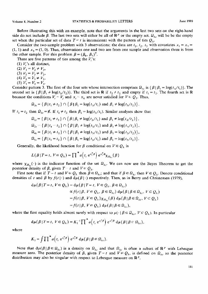
Before illustrating this with an example, note that the arguments in the last two sets on the right-hand side do not include p. The last two sets will either be all of R JJ or the empty set. 52,, will be be the empty set when the particular set of data T = t is inconsistent with the pattern of ties Q,.

Consider the two-sample problem with 3 observations; the data are t,, t,, t, with covariates x, = x2 = (1, 1) and x3 = (1, 0). Thus, observations one and two are from one sample and observation three is from the other sample. For this problem /3 = (&, &)T.

There are five patterns of ties among the v’s: (1) y’s all distinct, (2) I5 = v, + v,, (3) v, = v, + v,, (4) v, = v, + v,, (5) Vi = V, = V,.

Consider pattern 3. The first of the four sets whose intersection comprises O,, is { p 1 j?, = log( t/t,)}. The second set is { j3 1 PI # log(t,/t,)}. The third set is R if t, Z t, and empty if t, = t,. The fourth set is R because the conditions y = 5 and xi = xk are never satisfied for I/E Q,. Thus,

a,,={pltl#t2}n{(plP,=log(t3/t1)andP,#log(t,/t,))

If t, = t, then sl,, =fl. If t, # t, then pi = log(t,/t,). Similar analyses show that

~,,={~Ifl#f~}n{~IP1#log(t,/t,)andP,#log(t,/t,)},

fh,= {PItI=t2} n {PIP1+lod@d and&+hdt,/b)},

~n4t={PIfl#t,}n{pIP1#log(t,/t,)andP,=log(t,/t,)},

f&, = { P I 1, = t2 > n { P I PI = lodt,/t,) and PI = lo&,/t, I>.

Generally, the likelihood function for j3 conditional on VE QA is

L(fi I T= t, VE Q,) = n*a( ti ex:“) e”7BXn,,(/?)

where xc,,(.) is the indicator function of the set SL,,. We can now use the Bayes Theorem to get the posterior density of /3, given T = t and V E Q,.

First note that if T = t and V E QA then j3 E UL,,; and that if p E O,, then V/E Q,. Denote conditional densities of t and /3 by f(t I .) and dp(j3 1.) respectively. Then, as in Berry and Christensen (1979)

dp(P IT= t, VE Q,) = dp(P I T= t, P’E Qh, P E f&t)

af(t I P, VE Qh, P E %> +L(P IP 6 f&t, v= Q,)

=_f(t I Pp VE Q,>x,,,(P) +(P I P E 4, VE Q,>

=.f(t I P> VE Q,> dp(P I P E f&t)>

where the first equality holds almost surely with respect to p(. 1 p E LnXr, VE Q,). In particular

dp(@lT=t, V~Q,)=K;‘n*cz(t, ex’“) exfa dp(j?lj3E9,,),

Note that dp(P I j3 E a,,) is a density on 9,, and that a,, is often a subset of R p with Lebesgue measure zero. The posterior density of p, given T = t and VE Q,, is defined on 52,, so the posterior distribution may also be singular with respect to Lebesgue measure on Iw “.

181

Volume 8, Number 2 STATISTICS & PROBABILITY LETTERS June 1989

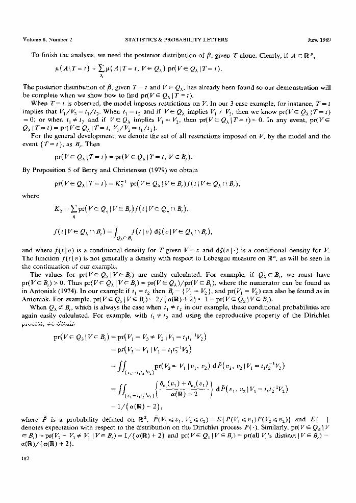
To finish the analysis, we need the postenor distribution of fi, given T alone. Clearly, if A c RP,

p(AIT=t)=xp(AIT=t, V~Q,)pr(l/~Q~l7’=?). x

The posterior distribution of p, given T = t and V E Q,, has already been found so our demonstration will be complete when we show how to find pr( V E Q, ) T = t).

When T = t is observed, the model imposes restrictions on V. In our 3 case example, for instance, T = t implies that Vi/V, = t,/r,. When t, = t, and if VE Q, implies Vi # V,, then we know pr( V E Qh 1 T = t)

= 0; or when t, f t, and if VE Qx implies Vi = V,, then pr(V’E Qx ( T = t) = 0. In any event, pr(VE Qh 1 T = t) = pr( VE Qx I T = t, VI/V, = fl/t2).

For the general development, we denote the set of all restrictions imposed on V, by the model and the event { T = t }, as B,. Then

pr(VEQX(T=t)=pr(VEQ,lT=t, VEB,).

By Proposition 5 of Berry and Christensen (1979) we obtain

pr(YEQhIT=t)=G1 pr(VEQhIVEB,)f(tl~/EQ,ng,),

where

K,=C~~(~/EQ~IVEB,)~(~IVEQ,~B,), 9

and where f( t I u) is a conditional density for T given V = u and dl( u ) .) is a conditional density for V. The function f(t ( u) is not generally a density with respect to Lebesgue measure on R”, as will be seen in the continuation of our example.

The values for pr(V E Qh ) I/ E B,) are easily calculated. For example, if Qh c B,, we must have pr( VE B,) > 0. Thus pr(VE Q, I VE B,) = pr( I/E Q*)/pr( VE B,), where the numerator can be found as in Antoniak (1974). In our example if t, = t, then B, = {Vi = V,}, and pr( V, = V,) can also be found as in Antoniak. For example, pr( V E Qs ) I/ E B,) = 2/{ cr(R) + 2) = 1 - pr( V E Q2 ) V E B,).

When Q, G B,, which is always the case when t, f t, in our example, these conditional probabilities are again easily calculated. For example, with f1 # t2 and using the reproductive property of the Dirichlet process, we obtain

pr(V~Q3)V~B,)=pr(Vl=V3fV2)Vl=tlt;1V2)

=pr(T/,=Vi IV,=t,t;‘V,)

= lJ ( u1 = t,t; bz)

pr(V3 = VI I q, u2> dj( u,, u2 IV, = t,t;‘&)

where i is a probability defined on R2, &V,<u,, V,~uu,)=E{P(V~“,uu,)P(V2/,uo,)} and E{ } denotes expectation with respect to the distribution on the Dirichlet process P(a). Similarly, pr( V E Q4 ) V

E B,) = pr( V2 = V3 Z Vi I VE B,) = l/{ a(R) + 2) and pr(VE Q, 1 VE B,) = pr(al1 y’s distinct I VE B,) =

oW{4~) + 2).

182

Volume 8, Number 2 STATISTICS & PROBABILITY LETI-ERS June 1989

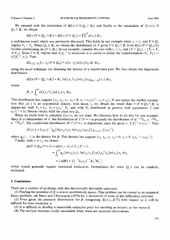
We proceed with the calculation of d{( u 1 VE Qh n B,), and finally to the calculation of f(t 1 u). If Q, c B,, we obtain

a well-known result which was previously discussed. This holds in our example when t, = t, and VE QA implies Vi = V,. When QA K B,, we obtain the distribution of V given VE Q, n B, from dS(u 1 VE Qx) by further conditioning on { V E B, }. In our example, consider the case with t, # t,, and { V E Q4 } = { V, = V, # Vi}. Since VE B, implies that V,V;’ is restricted, it is useful to define the transformation (V,, V,) + (V2Vze’, V2). Then

dL,v;l,v,(c, ~2 I VE Q,> = a(~> ~2)a(u,)u, dc du,,

using the usual technique for obtaining the density of a transformed pair. We thus obtain the degenerate distribution

dS(ulVE QJW) =K31,(t,t,‘u2)a(u2)u2~p,nB,(u2) do,,

where

K,=~ma(f,fr1u2)u(u2)u, du,.

This distribution has support { ul, u2, ug: u2 > 0, ul = u2tlt;‘, u3 = u2 }. If one makes the further assump- tion that a(.) is an exponential density, with mean 1, we obtain the result that V I T/E Q4 n B, is

degenerate with V, = V2, Vl = t,t;’ V, and with V, distributed as gamma with parameters 2 and (tit;’ + 1). Similar results hold for other sets QA.

When we know how to calculate f(t I u), we are done. We illustrate how to do this for our example. Since p is independent of V, the distribution of T I V = u is precisely the distribution of (e-“:flu,, epx:Bu2, e-X:Pu 3)T. The conditional distribution of T I V = u is degenerate, since for given u: T,T;’ = ulv;‘. Thus

At I u) = (t,t,)_lg,(ln(u,/r,), ln(v*t,/t,u,)}X~.,.i’)(t,t,‘),

where gp{ ., .} h d is t e ensity for p. This density has support {f,, t2, 1,: t, > 0, t, > 0, t,t;’ = v,v;'}.

Finally, with t, # t,, we obtain

pr(VEQ41T=t)=pr(V2=V,# V, IT=t)

=/P~p{ln(u2/h). ln(t,/t,)}a(t,t,‘u,)a(u,)u, du, 0

x {a(R) + 2) ~l(t,t,)-lK,‘K,‘,

which would generally require numerical evaluation. Probabilities for other Qx’s can be similarly evaluated.

3. Conclusions

There are a number of problems with this theoretically desireable approach: (1) Finding the posterior of p is almost prohibitively messy. This problem can be viewed as an empirical

Bayes problem; see Berry and Christensen (1979) for a discussion of some of the difficulties involved. (2) Even given the posterior distribution for p, integrating S(t I x, p T) with respect to it will be

difficult for even moderate p. (3) It is difficult to develop a reasonable subjective prior for anything as esoteric as the vector p. (4) The analysis becomes totally intractable when there are censored observations.

183

Volume 8. Number 2 STATISTICS & PROBABILITY LETTERS June 1989

Acknowledgement

Thanks to a careful referee for suggestions which improved the manuscript.

References

Antoniak, C.E. (1974), Mixtures of Dirichlet processes with applications to Bayesian nonparametric problems, Ann. Statist. 2, 1152-1174.

Berry, D. and R. Christensen (1979), Empirical Bayes estima- tion of a binomial parameter via mixtures of Dirichlet processes, Ann. Statist. 7, 558-568.

Burridge, J. (1981), Empirical Bayes analysis of survival times data, J. Roy. Statist. Sot. Ser. B 43, 65-75.

Christensen, R. and W. Johnson (1988), Modeling accelerated failure time with a Dirichlet process, Biometrika 75,

693-704. Cox, D.R. (1972) Regression models and life-tables, J. Roy.

Statist. Sot. Ser. B 34, 187-202.

Kalbfleisch, J.D. (1978), Nonparametric Bayesian analysis of survival time data, J. Roy. Statist. Sot. Ser. B 40, 214-221.

184