Embed Size (px)
Citation preview
University of Oxford
M.Sc. Mathematical Modelling andScientific Computing
Nonlinear Waves inGranular Lattices
Author:Michael P. Byrne
Supervisor:Dr Mason A. Porter
2009
Acknowledgements
I would like to thank my dissertation supervisor, Dr Mason Porter,
for his direction, suggestions and generous support throughout.
I would also like to acknowledge Dr Georgios Theocharis for his
helpful suggestions and for permission to use his code for the
simulations with discrete breathers.
This publication was based on work supported in part by Award
No KUK-C1-013-04 , made by King Abdullah University of Sci-
ence and Technology (KAUST).
Abstract
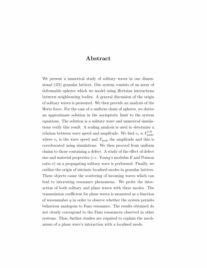
We present a numerical study of solitary waves in one dimen-
sional (1D) granular lattices. Our system consists of an array of
deformable spheres which we model using Hertzian interactions
between neighbouring bodies. A general discussion of the origin
of solitary waves is presented. We then provide an analysis of the
Hertz force. For the case of a uniform chain of spheres, we derive
an approximate solution in the asymptotic limit to the system
equations. The solution is a solitary wave and numerical simula-
tions verify this result. A scaling analysis is used to determine a
relation between wave speed and amplitude. We find vs ∝ F1/6peak,
where vs is the wave speed and Fpeak the amplitude and this is
corroborated using simulations. We then proceed from uniform
chains to those containing a defect. A study of the effect of defect
size and material properties (i.e. Young’s modulus E and Poisson
ratio ν) on a propagating solitary wave is performed. Finally, we
outline the origin of intrinsic localised modes in granular lattices.
These objects cause the scattering of incoming waves which can
lead to interesting resonance phenomena. We probe the inter-
action of both solitary and plane waves with these modes. The
transmission coefficient for plane waves is measured as a function
of wavenumber q in order to observe whether the system permits
behaviour analogous to Fano resonance. The results obtained do
not clearly correspond to the Fano resonances observed in other
systems. Thus, further studies are required to explain the mech-
anism of a plane wave’s interaction with a localised mode.
Contents
1 Introduction 1
2 Solitary Waves in Hertzian Chains 5
2.1 What is a Solitary Wave? . . . . . . . . . . . . . . . . . . . . 5
2.2 Wave Dispersion . . . . . . . . . . . . . . . . . . . . . . . . . 6
2.2.1 Non-Dispersive Waves . . . . . . . . . . . . . . . . . . 6
2.2.2 Dispersive Waves . . . . . . . . . . . . . . . . . . . . . 7
2.3 A Balance of Nonlinearity and Dispersion . . . . . . . . . . . . 9
2.4 Hertzian Chains . . . . . . . . . . . . . . . . . . . . . . . . . . 12
2.4.1 The Hertz Force . . . . . . . . . . . . . . . . . . . . . . 12
2.4.2 Equations of Motion and the Solitary Wave Solution . 15
2.5 Experimental Setup . . . . . . . . . . . . . . . . . . . . . . . . 18
2.6 Simulations and Results . . . . . . . . . . . . . . . . . . . . . 20
3 Defects in Granular Lattices 22
3.1 Overview of Granular Defects . . . . . . . . . . . . . . . . . . 22
3.2 Results and Discussion . . . . . . . . . . . . . . . . . . . . . . 24
3.2.1 Light and Heavy Defects . . . . . . . . . . . . . . . . . 25
3.2.2 The Effect of Young’s Modulus E and Poisson Ratio ν 28
4 Wave Interactions with Discrete Breathers 30
4.1 Introduction . . . . . . . . . . . . . . . . . . . . . . . . . . . . 30
4.2 The Phenomenon of Resonance . . . . . . . . . . . . . . . . . 30
4.3 Fano Resonance . . . . . . . . . . . . . . . . . . . . . . . . . . 32
4.3.1 The Fano-Anderson Model . . . . . . . . . . . . . . . . 35
4.4 Discrete Breathers . . . . . . . . . . . . . . . . . . . . . . . . 37
4.5 Results and Discussion . . . . . . . . . . . . . . . . . . . . . . 42
5 Conclusions 46
A Simulation Code 48
References 54
i
1 Introduction
This dissertation investigates the dynamics of a one dimensional chain of
spherical balls. The system can be modelled as a series of coupled nonlinear
oscillators, and as such exhibits many fascinating phenomena such as solitary
waves [22] and intrinsic localized modes [8]. Studies of nonlinear oscillator
chains began over fifty years ago with the Fermi-Pasta-Ulam (FPU) problem
and today it is still an active area of research [27].
One of the most interesting properties of these chains of nonlinear oscil-
lators is that they support the propagation of solitary waves. Waves of this
type are examples of nonlinear waves. Nonlinear waves have been studied
since the nineteenth century, for example by Stokes, Korteweg and deVries,
Boussinesq, and others [30]. Specifically, the solitary wave discovered exper-
imentally by John Scott Russell on a Scottish canal in the 1830s was shown
to be a solution to the following equation
ψt + (c0 + c1ψ)ψx + νψxxx = 0. (1.1)
In this equation, ψ denotes the displacement, the subscripts x and t indicate
partial derivatives with respect to those quantities, and c0, c1 and ν are
constants. This equation was initially introduced by Korteweg and deVries to
describe long waves in water of relatively shallow depth. However, Equation
(1.1), known as the KdV equation, has since been applied to other systems
due to it being one of the simplest equations to combine nonlinearity and
dispersion. The effect of these phenomena is discussed in detail in Chapter
2. However, the KdV equation is not alone in having solitary wave solutions
- the sine-Gordon and nonlinear Schrodinger equations have also been found
to yield such waves.
Solitary waves have been discovered in a variety of physical contexts,
from optics to waterways and many others. A recently observed occurrence
is in a system of discrete, barely touching spheres which interact via the
nonlinear Hertz force (see Section 2.4.1). Solitary waves in these Hertzian
lattices were first investigated by Nesterenko [23] and have since been probed
by experiments [3], numerical simulations [12], and by analytical calculations
[2]. Such a system is of interest for a variety of reasons: from understanding
1
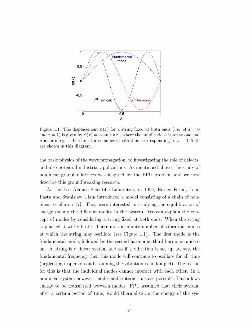
Figure 1.1: The displacement ψ(x) for a string fixed at both ends (i.e. at x = 0and x = 1) is given by ψ(x) = A sin(nπx), where the amplitude A is set to one andn is an integer. The first three modes of vibration, corresponding to n = 1, 2, 3,are shown in this diagram.
the basic physics of the wave propagation, to investigating the role of defects,
and also potential industrial applications. As mentioned above, the study of
nonlinear granular lattices was inspired by the FPU problem and we now
describe this groundbreaking research.
At the Los Alamos Scientific Laboratory in 1955, Enrico Fermi, John
Pasta and Stanislaw Ulam introduced a model consisting of a chain of non-
linear oscillators [7]. They were interested in studying the equilibration of
energy among the different modes in the system. We can explain the con-
cept of modes by considering a string fixed at both ends. When the string
is plucked it will vibrate. There are an infinite number of vibration modes
at which the string may oscillate (see Figure 1.1). The first mode is the
fundamental mode, followed by the second harmonic, third harmonic and so
on. A string is a linear system and so if a vibration is set up at, say, the
fundamental frequency then this mode will continue to oscillate for all time
(neglecting dispersion and assuming the vibration is undamped). The reason
for this is that the individual modes cannot interact with each other. In a
nonlinear system however, mode-mode interactions are possible. This allows
energy to be transferred between modes. FPU assumed that their system,
after a certain period of time, would thermalise i.e the energy of the sys-
2
tem would eventually be equipartioned between all the modes in the system.
However, after running simulations on their system they did not observe
equipartioning. To the astonishment of the researchers, the results showed
that although energy was initially shared between a number of modes, after
a period of time the system returned to a state that was close to the initial
state. In the 1960s the connection between the FPU problem and the work
performed on nonlinear waves by Korteweg-de Vries and others, was made
by Norman Zabusky and Martin Kruskal. Introducing a continuum model
of the FPU system, they realised that the partial differential equation de-
scribing the motion of the system was, in fact, the KdV equation which had
originally been derived more than sixty years previously. The solutions they
found were a particular type of solitary wave which they called a soliton1.
Although the motion of solitons in an FPU chain can be quite regular, the
system can also show chaotic behaviour depending on the initial conditions.
If the energy provided to the system is sufficiently high then chaos can al-
low energy to be transferred between modes leading to equipartition. The
complex behaviour and striking nonlinear effects observable in this seemingly
simple system have inspired extensive research and this problem is still being
investigated today [26].
Our investigations will begin with a system that is very similar to the
original FPU setup. We will examine the properties of a uniform chain of
spheres. The Hertz force will be introduced and an approximate solution to
the equations of motion of the system will be derived. We will also solve the
system numerically.
In Chapter 3, we introduce a defect to our lattice. Such impurities can
dramatically alter the behaviour of the granular chain. Using numerical
simulations, we vary the properties of this defect and investigate the effects
on the propagation of the solitary wave.
In addition to solitary waves, Hertzian systems have also been shown to
support intrinsic localised modes (ILMs), which are also known as discrete
breathers (DBs) [28]. These are spatially localised solutions to the equations
of motion which arise due to the combination of nonlinearity and discreteness
1The commonly used term soliton is a special case of a solitary wave. Solitons have anadditional amazing property which is that if two solitons collide they retain their propertiesand emerge intact [19].
3
in the system (see Section 4.3). Chapter 4 focuses on the interaction of
solitary and plane waves with a DB. Motivated by the observation of Fano
resonances in waveguide arrays [21], we numerically investigate the possibility
of a nonlinear “Fano-like” resonance due to the interaction of plane waves
with the DB. We term such a resonance as Fano-like because Fano resonance
itself is a linear phenomenon, this will be explored further in Chapter 4.
We end with our conclusions followed by the Appendices which contain
the Matlab codes used to perform the simulations for Chapters 2 and 3.
4
2 Solitary Waves in Hertzian Chains
2.1 What is a Solitary Wave?
In this chapter, we will begin by introducing the concept of nonlinear waves
and explaining how they arise. Following that, a description of the granular
lattice system that is the focus of this dissertation will be given. We will then
derive an approximate solution to the system’s equations of motion before
presenting the results of numerical simulations. In addition, we include a brief
discussion of the techniques used to investigate these systems experimentally.
As mentioned in Chapter 1, a 1D chain of spherical balls may support the
propagation of a solitary wave. Solitary waves are fundamentally different
to most of the waves we encounter in everyday life. Most waves, such as
sound waves and electromagnetic waves, are linear waves. Linear waves are
characterised by having a return force which is linearly dependent on the
displacement. Solitary waves, however, are nonlinear waves - the return force
is not directly proportional to the displacement from equilibrium [19]. This
can be illustrated more clearly by considering the equation for a sinusoidal
travelling wave, which we write as
u(x, t) = A sin(qx− ωt+ φ) (2.1)
where u is the displacement from equilibrium, A is the wave amplitude, q
the wave number, ω the angular frequency and φ an initial phase shift. We
know that ω = vq where v is the wave speed. An important point to note
is that Equation (2.1) is a solution to the equation for a harmonic oscillator,
i.e.
u(x, t) ≡ d2u
dt2= −ω2u(x, t) (2.2)
where the dot represents the derivative with respect to time. This equation
shows that the restoring force is linearly dependent on the displacement.
Another important property of linear waves is that the wave speed is in-
dependent of the wave amplitude, it depends only on the properties of the
material through which it passes [27].
However, not all return forces are linear. We will consider nonlinear forces
of the form
5
u = k(uα), α > 1 (2.3)
where k is a constant. Such nonlinear forces, combined with a phenomenon
known as dispersion (we will give a detailed discussion of dispersion in Section
2.2) can allow solitary waves to propagate in a given medium and this will
be illustrated in Section 2.3.
2.2 Wave Dispersion
In order to understand the origin of solitary waves, we must explain the
phenomenon of dispersion. A dispersive system is one in which the velocity
of a wave depends on its frequency. This dependence is expressed by a
dispersion relation that relates ω to q for a particular system.
2.2.1 Non-Dispersive Waves
First, we will consider non-dispersive waves. The non-dispersive wave equa-
tion is written as
∂2u
∂t2= v2∂
2u
∂x2. (2.4)
This equation admits travelling wave solutions. A particular class of these
solutions are sinusoidal travelling waves, an example of which is given by
Equation (2.1). Sinusoidal travelling waves are just a subset of the d’Alembert
solutions to Equation (2.4). D’Alembert’s general solution to Equation (2.4)
is written as
u(x, t) = F (x+ vt) +G(x− vt) (2.5)
where F and G are functions. This solution is interpreted as two waves with
speed v moving in opposite directions along the x-axis.
We use sinusoidal waves as an example to highlight the properties of
non-dispersive systems. These solutions can also be expressed as
u(x, t) = C exp[i(ωt− qx)] + C∗ exp[−i(ωt− qx)] (2.6)
where C is a constant (with complex conjugate C∗). Inserting this expression
into Equation (2.4) we see that in order for the solution to be valid, ω and
6
q must satisfy ω = ±vq. If we consider waves described by Equation (2.6)
to be travelling along a piece of string, for instance, then it is obvious that
each point on the string vibrates at the same angular frequency ω. Another
important property of these waves is the phase velocity vφ. For sinusoidal
travelling waves, vφ is given by [19]
dx
dt=ω
q≡ vφ. (2.7)
This quantity describes the velocity at which the entire wave profile moves.
For the waves we are currently discussing, vφ depends only on the properties
of the medium and not on the properties of the wave itself, such as its fre-
quency. For a sinusoidal travelling wave, constant values of the phase angle
move either to the left or to the right (if we consider a string, for example)
with a velocity v. As d’Alemberts solution (2.5) shows, this behaviour can
be generalized to non-sinusoidal waves which do not undergo harmonic vi-
brations. We now note that the phase angle will remain constant as long
as the variable Z ≡ x ± vt does so [19]. Any function u(x, t) in which x
and t appear only in the form x± vt will satisfy Equation (2.4) and also the
relation
∂u
∂t± v
(∂u
∂x
)= 0. (2.8)
This shows that any disturbance of the string from its equilibrium shape
may propagate along the string, with the entire waveform moving at velocity
v and thus not distorting its shape over space and time. This property of
non-dispersion is unique to Equation (2.4) and a system which obeys this
equation is said to be non-dispersive. An example of a physical system that
approximately obeys Equation (2.4) are longitudinal disturbances of a gas
within a cylinder (an example of an acoustic wave) [19].
2.2.2 Dispersive Waves
Non-dispersive waves are very special however. Returning to our example of
a string, when we described this system as non-dispersive we assumed that
the string was perfectly flexible, i.e. that the only transverse force was due
to tension. However, real strings are ‘stiff’, in that they tend to straighten
7
themselves even in the absence of tension. This additional force adds a
higher order term to Equation (2.4) and makes the system dispersive. By
considering the forces acting on a stiff string, we write the following equation
[19]
∂2u
∂t2= v2
(∂2u
∂x2− α∂
4u
∂x4
), (2.9)
where α is a positive constant dependent on the shape of the cross-section
and the elasticity of the string. We compare this to the non-dispersive wave
equation (2.4) and note the additional higher order term. We wish to know
whether such a system can still support the propagation of a travelling wave
and so we substitute the expression (2.6) for a sinusoidal travelling wave into
Equation (2.9) and find that ω and q must satisfy the following dispersion
relation
ω = ±vq(1 + αq2)1/2. (2.10)
For a perfectly flexible string (i.e. α = 0), this relation reduces to ω = vq
which is the dispersion relation for the non-dispersive systems we previ-
ously described. For a slightly stiff string with a wavelength that is not
too small, αq2 1 and we can write Equation (2.10) in the approximate
form ω ≈ ±vq(1 + 12αq2). We rewrite this expression as ω = cq − dq3, which
is an expression for the dispersion relation of a slightly dispersive system.
Substituting the equation for a sinusoidal travelling wave into this dispersion
relation, we can convert Equation (2.9) into
∂u
∂t+ v
(∂u
∂x
)+ d
(∂3u
∂x3
)= 0. (2.11)
This is an example of a travelling wave equation for a slightly dispersive
system. We may use the dispersion relation (2.10) to determine the phase
velocity vφ as we did for non-dispersive systems (see Equation (2.7)). For
the dispersive system we are considering, vφ is given by
|vφ| = v(1 + αq2)1/2. (2.12)
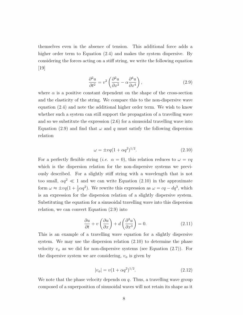
We note that the phase velocity depends on q. Thus, a travelling wave group
composed of a superposition of sinusoidal waves will not retain its shape as it
8
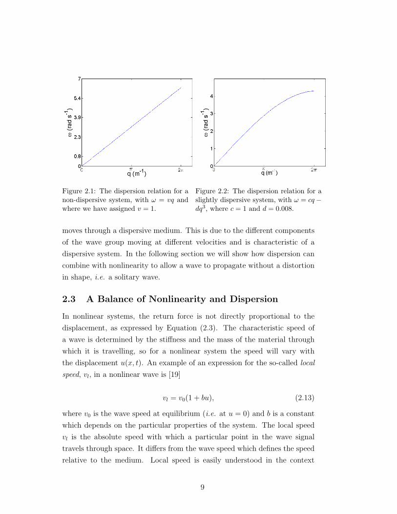
Figure 2.1: The dispersion relation for anon-dispersive system, with ω = vq andwhere we have assigned v = 1.
Figure 2.2: The dispersion relation for aslightly dispersive system, with ω = cq−dq3, where c = 1 and d = 0.008.
moves through a dispersive medium. This is due to the different components
of the wave group moving at different velocities and is characteristic of a
dispersive system. In the following section we will show how dispersion can
combine with nonlinearity to allow a wave to propagate without a distortion
in shape, i.e. a solitary wave.
2.3 A Balance of Nonlinearity and Dispersion
In nonlinear systems, the return force is not directly proportional to the
displacement, as expressed by Equation (2.3). The characteristic speed of
a wave is determined by the stiffness and the mass of the material through
which it is travelling, so for a nonlinear system the speed will vary with
the displacement u(x, t). An example of an expression for the so-called local
speed, vl, in a nonlinear wave is [19]
vl = v0(1 + bu), (2.13)
where v0 is the wave speed at equilibrium (i.e. at u = 0) and b is a constant
which depends on the particular properties of the system. The local speed
vl is the absolute speed with which a particular point in the wave signal
travels through space. It differs from the wave speed which defines the speed
relative to the medium. Local speed is easily understood in the context
9
of longitudinal waves where the medium moves back and forth along the
direction of propagation with an instantaneous speed u. If we denote the
wave speed as c then the local velocity can be written as vl = c+u. Assuming
the dispersion is negligible, the derivative u is in phase with the displacement
u which leads to the approximate form of vl given by Equation (2.13).
As described previously in the case of a linear system, in order for a signal
to travel undistorted in the positive x direction the displacement u(x, t) must
be a function of vt−x and must satisfy Equation (2.8). For a nonlinear system
with a wave velocity which varies as in Equation (2.13), the following holds:
∂u
∂t+ v0(1 + bu)
∂u
∂x= 0. (2.14)
Neglecting dispersion, nonlinearity causes a signal to be distorted as it moves
through the material. If we add dispersion to the system, it might seem rea-
sonable to assume that a material which is both dispersive and nonlinear
is likely to distort the shape of a signal. However, dispersion and nonlin-
earity can sometimes cancel each other out, allowing a stable waveform to
propagate indefinitely. We return to Equation (2.11), the wave equation for
a slightly dispersive system, and substitute in Equation (2.14) containing
the nonlinear term. This gives us the following wave equation which ap-
proximately describes the propagation of a wave in a slightly nonlinear and
slightly dispersive material
∂u
∂t+ v0(1 + bu)
∂u
∂x+ d
(∂3u
∂x3
)= 0. (2.15)
The equation above is in fact an expression of the KdV equation, initially
introduced in Chapter 1 (see Equation (1.1)). This equation may be solved
by a particular type of travelling wave, a solitary wave.
As shown previously, for a waveform u(x, t) to propagate without any
distortion of its shape, u must be a function of the variable Z. Using Z, we
transform Equation (2.15) from a partial differential equation (PDE) to an
ordinary differential equation (ODE), yielding
(v − v0)u′ − bv0uu′ − du′′′ = 0, u′ ≡ du
dZ. (2.16)
Directly integrating this equation twice gives
10
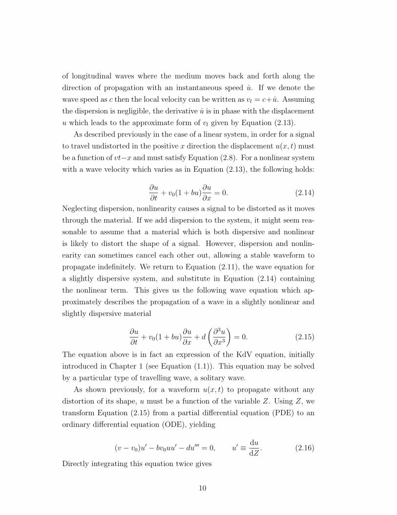
Figure 2.3: A plot of Equation (2.17)which is a solitary wave solution. Wehave set the constants β and γ equal toone.
Figure 2.4: A schematic diagram showingtwo neighbouring spheres under compres-sion. The spheres repel each other via theHertz force F , where F ∝ δ3/2
i,i+1.
1
2(v − v0)u2 − 1
6bv0u
3 − 1
2du′2 + Cu+D = 0,
where C and D are constants of integration. Assuming that our solitary
wave solution is localised, we require C = D = 0 to ensure that u, u′ → 0 as
Z → ±∞. We can now rewrite the equation as
du′2 = (v − v0 −1
3bv0u)u2.
The equation may be simplified to
(u′)2 = (A−Bu)u2
where A = (v − v0)/d and B = bv0/3d. This ODE has the solution
u = β sech2(γZ) (2.17)
where β = A/B and γ = 12A1/2. This is the solitary wave solution and is
plotted in Figure 2.3. Using the condition for a maximum (i.e. u′ = 0) we
can also deduce the wave speed v = v0(1+ 13bumax). Equation (2.17) gives us a
simple qualitative understanding of the effect of dispersion and nonlinearity
on our solitary wave: The more dispersive the medium (i.e larger d) the
11
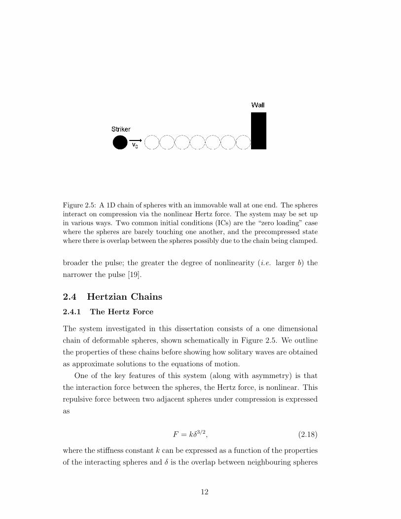
Figure 2.5: A 1D chain of spheres with an immovable wall at one end. The spheresinteract on compression via the nonlinear Hertz force. The system may be set upin various ways. Two common initial conditions (ICs) are the “zero loading” casewhere the spheres are barely touching one another, and the precompressed statewhere there is overlap between the spheres possibly due to the chain being clamped.
broader the pulse; the greater the degree of nonlinearity (i.e. larger b) the
narrower the pulse [19].
2.4 Hertzian Chains
2.4.1 The Hertz Force
The system investigated in this dissertation consists of a one dimensional
chain of deformable spheres, shown schematically in Figure 2.5. We outline
the properties of these chains before showing how solitary waves are obtained
as approximate solutions to the equations of motion.
One of the key features of this system (along with asymmetry) is that
the interaction force between the spheres, the Hertz force, is nonlinear. This
repulsive force between two adjacent spheres under compression is expressed
as
F = kδ3/2, (2.18)
where the stiffness constant k can be expressed as a function of the properties
of the interacting spheres and δ is the overlap between neighbouring spheres
12
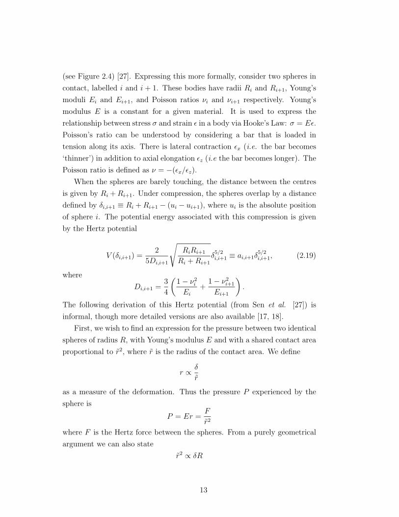
(see Figure 2.4) [27]. Expressing this more formally, consider two spheres in
contact, labelled i and i + 1. These bodies have radii Ri and Ri+1, Young’s
moduli Ei and Ei+1, and Poisson ratios νi and νi+1 respectively. Young’s
modulus E is a constant for a given material. It is used to express the
relationship between stress σ and strain ε in a body via Hooke’s Law: σ = Eε.
Poisson’s ratio can be understood by considering a bar that is loaded in
tension along its axis. There is lateral contraction εx (i.e. the bar becomes
‘thinner’) in addition to axial elongation εz (i.e the bar becomes longer). The
Poisson ratio is defined as ν = −(εx/εz).
When the spheres are barely touching, the distance between the centres
is given by Ri +Ri+1. Under compression, the spheres overlap by a distance
defined by δi,i+1 ≡ Ri +Ri+1 − (ui − ui+1), where ui is the absolute position
of sphere i. The potential energy associated with this compression is given
by the Hertz potential
V (δi,i+1) =2
5Di,i+1
√RiRi+1
Ri +Ri+1
δ5/2i,i+1 ≡ ai,i+1δ
5/2i,i+1, (2.19)
where
Di,i+1 =3
4
(1− ν2
i
Ei+
1− ν2i+1
Ei+1
).
The following derivation of this Hertz potential (from Sen et al. [27]) is
informal, though more detailed versions are also available [17, 18].
First, we wish to find an expression for the pressure between two identical
spheres of radius R, with Young’s modulus E and with a shared contact area
proportional to r2, where r is the radius of the contact area. We define
r ∝ δ
r
as a measure of the deformation. Thus the pressure P experienced by the
sphere is
P = Er =F
r2
where F is the Hertz force between the spheres. From a purely geometrical
argument we can also state
r2 ∝ δR
13
Combining the above expressions, we find that
E
(δ
r
)∝ F
δR⇒ E
(δ
R
)1/2
∝ F
δR.
Thus,
F ∝ ER1/2δ3/2.
We note the force is proportional to δ3/2, which is characteristic of the Hertz
law. Force is related to potential via the relation F = −dV/dδ, so
VHertz(δ) ∝ ER1/2δ5/2.
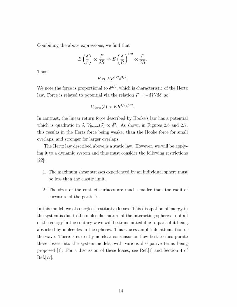
In contrast, the linear return force described by Hooke’s law has a potential
which is quadratic in δ, VHooke(δ) ∝ δ2. As shown in Figures 2.6 and 2.7,
this results in the Hertz force being weaker than the Hooke force for small
overlaps, and stronger for larger overlaps.
The Hertz law described above is a static law. However, we will be apply-
ing it to a dynamic system and thus must consider the following restrictions
[22]:
1. The maximum shear stresses experienced by an individual sphere must
be less than the elastic limit.
2. The sizes of the contact surfaces are much smaller than the radii of
curvature of the particles.
In this model, we also neglect restitutive losses. This dissipation of energy in
the system is due to the molecular nature of the interacting spheres - not all
of the energy in the solitary wave will be transmitted due to part of it being
absorbed by molecules in the spheres. This causes amplitude attenuation of
the wave. There is currently no clear consensus on how best to incorporate
these losses into the system models, with various dissipative terms being
proposed [1]. For a discussion of these losses, see Ref.[1] and Section 4 of
Ref.[27].
14
Figure 2.6: This plot shows a comparisonof F (δ) for Hooke’s law and Hertz’s law.We see that for small δ, FHooke > FHertz
but the opposite is true at larger δ.
Figure 2.7: V (δ) for the Hooke and Hertzpotentials. For lower δ, the Hooke systemcontains more potential energy but this isreversed for higher values of δ.
2.4.2 Equations of Motion and the Solitary Wave Solution
We now use the Hertz force to model the dynamics of our 1D granular lattice.
A system of N identical interacting spheres can be described with a set of
coupled nonlinear equations. We can write down the equation of motion for
the ith sphere as
miui = Ai−1,i(∆ + ui−1 − ui)3/2+ − Ai,i+1(∆ + ui − ui+1)
3/2+ , (2.20)
where Ai,i+1 ≡ (5/2)ai,i+1, ∆ arises due to an initial precompression, and the
index + indicates that the Hertz force is zero when the spheres are not in
contact [27]. An approximate solution to this system was first obtained by
Nesterenko [23]. Here we present a version of this solution used initially by
Chatterjee [2].
First, we are considering a chain of identical spheres so the force constants
Ai,i+1 are the same for 1 ≤ i ≤ N − 1. We denote this value k. The masses
are also identical so mi ≡ m, 1 ≤ i ≤ N . We are also going to assume there
is no precompression (i.e. the “zero loading” case) and thus ∆ = 0. Systems
such as this, where there is no linear force term, are known as “strongly
nonlinear”. We can now rewrite Equation (2.20) as
15
¨ui = (ui−1 − ui−1)3/2 − (ui − ui+1)3/2, 1 < i < N (2.21)
where ui(t) ≡ (k/m)2ui(t). In order to establish our solution, we assume that
when the chain of spheres is perturbed, this disturbance travels as a solitary
wave. Thus, the displacement of each sphere can be described by the same
function, albeit one which must be calculated at different times as the wave
moves through the chain. By this consideration, we can write
ui(t) = ui+1(t+ b), (2.22)
where b > 0 is a constant. Using Equation (2.22) and choosing an arbi-
trary sphere as a reference, we can rewrite Equation (2.21) in terms of the
displacement of this sphere as
¨u = [u(t+ b)− u(t)]3/2 − [u(t)− u(t− b)]3/2. (2.23)
Performing a power series expansion of u(t+ b), we obtain
u(t+ b) = u(t) + bdu
dt+b2
2!
d2u
dt2+ . . . .
We note at this point that we may also formulate this approximate solution
using a long-wavelength approximation, where it is assumed that the char-
acteristic spatial size of the perturbation is much greater than the distance
between spheres. This approach is taken by Nesterenko [23], Porter et al.
[25], and others.
Substituting the above expression into Equation (2.23) and then expand-
ing in powers of b we obtain
d2u
dt2=
3
2b5/2
√du
dt
d2u
dt2+
1
8b9/2
√du
dt
d4u
dt4
+1
8b9/2 d2u/dt2√
du/dt
+1
64b9/2 (d2u/dt2)3
(du/dt)3/2+O(b13/2).
(2.24)
We now truncate our series by ignoring terms of order O(b13/2) and higher.
We note that this is not mathematically rigorous, we are just attempting
16
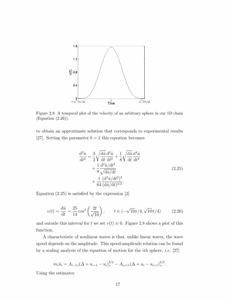
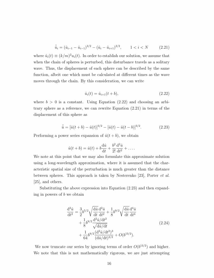
Figure 2.8: A temporal plot of the velocity of an arbitrary sphere in our 1D chain(Equation (2.26)).
to obtain an approximate solution that corresponds to experimental results
[27]. Setting the parameter b = 1 this equation becomes
d2u
dt2=
3
2
√du
dt
d2u
dt2+
1
8
√du
dt
d4u
dt4
+1
8
d2u/dt2√du/dt
+1
64
(d2u/dt2)3
(du/dt)3/2.
(2.25)
Equation (2.25) is satisfied by the expression [2]
v(t) =du
dt=
25
14cos4
(2t√10
), t ∈ (−
√10π/4,
√10π/4) (2.26)
and outside this interval for t we set v(t) ≡ 0. Figure 2.8 shows a plot of this
function.
A characteristic of nonlinear waves is that, unlike linear waves, the wave
speed depends on the amplitude. This speed-amplitude relation can be found
by a scaling analysis of the equation of motion for the ith sphere, i.e. [27]
miui = Ai−1,i(∆ + ui−1 − ui)3/2+ − Ai,i+1(∆ + ui − ui+1)
3/2+ .
Using the estimates
17
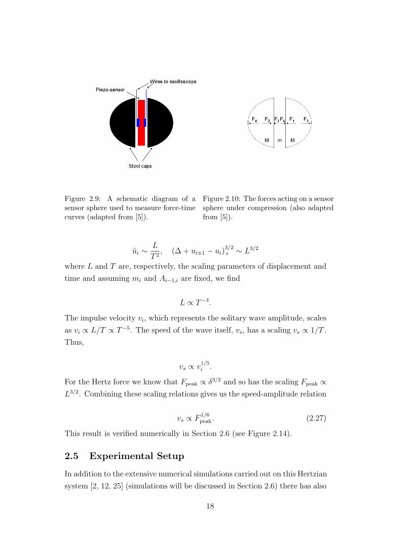
Figure 2.9: A schematic diagram of asensor sphere used to measure force-timecurves (adapted from [5]).
Figure 2.10: The forces acting on a sensorsphere under compression (also adaptedfrom [5]).
ui ∼L
T 2, (∆ + ui±1 − ui)3/2
+ ∼ L3/2
where L and T are, respectively, the scaling parameters of displacement and
time and assuming mi and Ai−1,i are fixed, we find
L ∝ T−4.
The impulse velocity vi, which represents the solitary wave amplitude, scales
as vi ∝ L/T ∝ T−5. The speed of the wave itself, vs, has a scaling vs ∝ 1/T .
Thus,
vs ∝ v1/5i .
For the Hertz force we know that Fpeak ∝ δ3/2 and so has the scaling Fpeak ∝L3/2. Combining these scaling relations gives us the speed-amplitude relation
vs ∝ F1/6peak. (2.27)
This result is verified numerically in Section 2.6 (see Figure 2.14).
2.5 Experimental Setup
In addition to the extensive numerical simulations carried out on this Hertzian
system [2, 12, 25] (simulations will be discussed in Section 2.6) there has also
18
Figure 2.11: A schematic diagram of an experimental setup to investigate a 1Dlattice with zero loading. The striker impacts the end of the chain with a velocityvinit sending a nonlinear wave propagating through the chain. The force at variouspoints is measured using piezo-sensors embedded within spheres and is relayed tothe oscilloscope. Figure adapted from Ref.[14].
been significant experimental work performed [15, 14, 25]. In this section we
provide a brief account of the experimental methods used.
Figure 2.11 shows the setup for a zero loading experiment. Force-time
measurements are made using piezo-sensors connected to oscilloscopes [25].
Whereas for numerical simulations a system consisting of hundreds of spheres
may be investigated; experimentalists are restricted to using smaller chains.
For instance, Job et al. use a maximum of fifty spheres [14] whilst Daraio et
al. investigate chains of seventy to eighty spheres [25]. Experimental setups
vary depending on the goals of the specific research, but it is typical to use
sensors to measure the force versus time for several spheres in the lattice. The
wave speed can also be obtained through “time-of-flight” measurements. One
technique for incorporating the sensor into the system is to insert it into the
middle of a sphere which has been sliced in half. It is important that the
properties of this “sensor sphere”, such as its mass and stiffness, are almost
identical to those of the other spheres in the lattice. Figure 2.9 is a schematic
diagram of a sensor sphere. In order to compare numerical and experimental
studies of the system, it is important to relate the forces measured by the
sensors to those calculated during simulations. This is described extensively
by Daraio et al. [5] and the following discussions are based on those in that
19
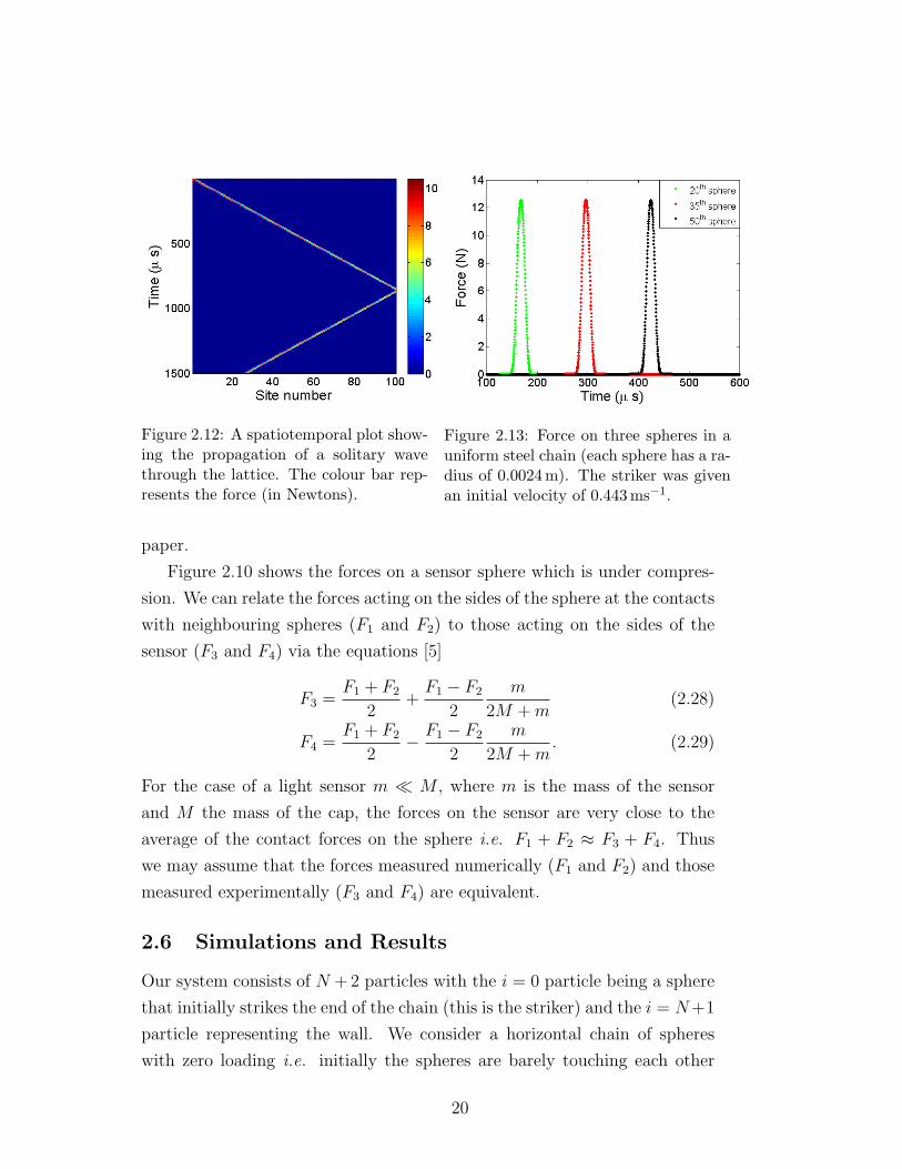
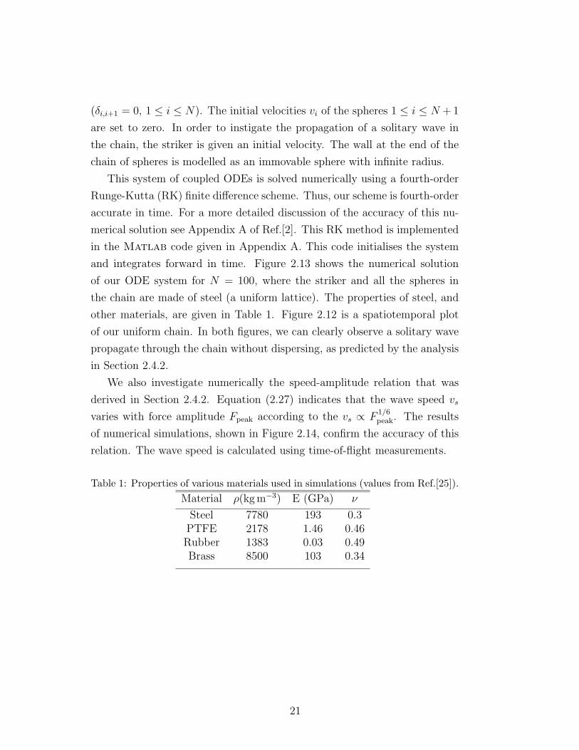
Figure 2.12: A spatiotemporal plot show-ing the propagation of a solitary wavethrough the lattice. The colour bar rep-resents the force (in Newtons).
Figure 2.13: Force on three spheres in auniform steel chain (each sphere has a ra-dius of 0.0024 m). The striker was givenan initial velocity of 0.443 ms−1.
paper.
Figure 2.10 shows the forces on a sensor sphere which is under compres-
sion. We can relate the forces acting on the sides of the sphere at the contacts
with neighbouring spheres (F1 and F2) to those acting on the sides of the
sensor (F3 and F4) via the equations [5]
F3 =F1 + F2
2+F1 − F2
2
m
2M +m(2.28)
F4 =F1 + F2
2− F1 − F2
2
m
2M +m. (2.29)
For the case of a light sensor m M , where m is the mass of the sensor
and M the mass of the cap, the forces on the sensor are very close to the
average of the contact forces on the sphere i.e. F1 + F2 ≈ F3 + F4. Thus
we may assume that the forces measured numerically (F1 and F2) and those
measured experimentally (F3 and F4) are equivalent.
2.6 Simulations and Results
Our system consists of N + 2 particles with the i = 0 particle being a sphere
that initially strikes the end of the chain (this is the striker) and the i = N+1
particle representing the wall. We consider a horizontal chain of spheres
with zero loading i.e. initially the spheres are barely touching each other
20
(δi,i+1 = 0, 1 ≤ i ≤ N). The initial velocities vi of the spheres 1 ≤ i ≤ N + 1
are set to zero. In order to instigate the propagation of a solitary wave in
the chain, the striker is given an initial velocity. The wall at the end of the
chain of spheres is modelled as an immovable sphere with infinite radius.
This system of coupled ODEs is solved numerically using a fourth-order
Runge-Kutta (RK) finite difference scheme. Thus, our scheme is fourth-order
accurate in time. For a more detailed discussion of the accuracy of this nu-
merical solution see Appendix A of Ref.[2]. This RK method is implemented
in the Matlab code given in Appendix A. This code initialises the system
and integrates forward in time. Figure 2.13 shows the numerical solution
of our ODE system for N = 100, where the striker and all the spheres in
the chain are made of steel (a uniform lattice). The properties of steel, and
other materials, are given in Table 1. Figure 2.12 is a spatiotemporal plot
of our uniform chain. In both figures, we can clearly observe a solitary wave
propagate through the chain without dispersing, as predicted by the analysis
in Section 2.4.2.
We also investigate numerically the speed-amplitude relation that was
derived in Section 2.4.2. Equation (2.27) indicates that the wave speed vs
varies with force amplitude Fpeak according to the vs ∝ F1/6peak. The results
of numerical simulations, shown in Figure 2.14, confirm the accuracy of this
relation. The wave speed is calculated using time-of-flight measurements.
Table 1: Properties of various materials used in simulations (values from Ref.[25]).Material ρ(kg m−3) E (GPa) ν
Steel 7780 193 0.3PTFE 2178 1.46 0.46Rubber 1383 0.03 0.49Brass 8500 103 0.34
21
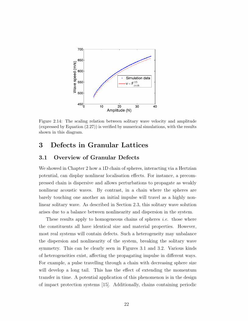
Figure 2.14: The scaling relation between solitary wave velocity and amplitude(expressed by Equation (2.27)) is verified by numerical simulations, with the resultsshown in this diagram.
3 Defects in Granular Lattices
3.1 Overview of Granular Defects
We showed in Chapter 2 how a 1D chain of spheres, interacting via a Hertzian
potential, can display nonlinear localisation effects. For instance, a precom-
pressed chain is dispersive and allows perturbations to propagate as weakly
nonlinear acoustic waves. By contrast, in a chain where the spheres are
barely touching one another an initial impulse will travel as a highly non-
linear solitary wave. As described in Section 2.3, this solitary wave solution
arises due to a balance between nonlinearity and dispersion in the system.
These results apply to homogeneous chains of spheres i.e. those where
the constituents all have identical size and material properties. However,
most real systems will contain defects. Such a heterogeneity may unbalance
the dispersion and nonlinearity of the system, breaking the solitary wave
symmetry. This can be clearly seen in Figures 3.1 and 3.2. Various kinds
of heterogeneities exist, affecting the propagating impulse in different ways.
For example, a pulse travelling through a chain with decreasing sphere size
will develop a long tail. This has the effect of extending the momentum
transfer in time. A potential application of this phenomenon is in the design
of impact protection systems [15]. Additionally, chains containing periodic
22
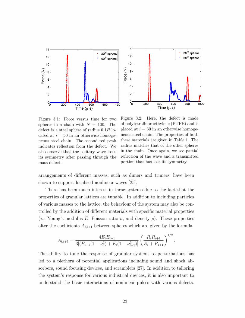
Figure 3.1: Force versus time for twospheres in a chain with N = 100. Thedefect is a steel sphere of radius 0.1R lo-cated at i = 50 in an otherwise homoge-neous steel chain. The second red peakindicates reflection from the defect. Wealso observe that the solitary wave losesits symmetry after passing through themass defect.
Figure 3.2: Here, the defect is madeof polytetrafluoroethylene (PTFE) and isplaced at i = 50 in an otherwise homoge-neous steel chain. The properties of boththese materials are given in Table 1. Theradius matches that of the other spheresin the chain. Once again, we see partialreflection of the wave and a transmittedportion that has lost its symmetry.
arrangements of different masses, such as dimers and trimers, have been
shown to support localised nonlinear waves [25].
There has been much interest in these systems due to the fact that the
properties of granular lattices are tunable. In addition to including particles
of various masses to the lattice, the behaviour of the system may also be con-
trolled by the addition of different materials with specific material properties
(i.e Young’s modulus E, Poisson ratio ν, and density ρ). These properties
alter the coefficients Ai,i+1 between spheres which are given by the formula
Ai,i+1 =4EiEi+1
3[(Ei+1(1− ν2i ) + Ei(1− ν2
i+1)]
(RiRi+1
Ri +Ri+1
)1/2
.
The ability to tune the response of granular systems to perturbations has
led to a plethora of potential applications including sound and shock ab-
sorbers, sound focusing devices, and scramblers [27]. In addition to tailoring
the system’s response for various industrial devices, it is also important to
understand the basic interactions of nonlinear pulses with various defects.
23

Figure 3.3: A spatio-temporal plot show-ing the propagation of a solitary wavethrough a lattice that contains a lightdefect located at site 100 (Rdefect =0.1Rchain, where Rdefect is the defect ra-dius and Rchain is the radius of the otherspheres in the chain). We note the sec-ondary waves that are created when thesolitary wave interacts with the defect.
Figure 3.4: Plotted above is the displace-ment of the light defect in an otherwisehomogeneous chain. We observe that thepropagating solitary wave causes the de-fect to shift suddenly and then oscillaterapidly. These oscillations cause the de-fect to collide with neighbouring spheres,creating the secondary waves we see inFigure 3.3.
Such an understanding can enable us to probe the internal composition of
solid objects in a nondestructive manner [13].
It is the impact of the size and material properties of defects on wave
propagation in Hertzian lattices that is the primary focus of this chapter.
We perform numerical simulations that probe the effect of different defects
on the properties of the solitary wave that propagates through the chain.
These results are presented below.
3.2 Results and Discussion
Initially we consider a steel defect of varying size in an otherwise homo-
geneous chain of steel spheres. The behaviour of the granular system is
remarkably different depending on whether the impurity is larger or smaller
than the other spheres in the chain. We now examine both these cases [12].
24
3.2.1 Light and Heavy Defects
As we just alluded to, a granular lattice with an embedded defect will show
very different behaviour depending on the size of that defect. These differ-
ences manifest themselves as different patterns of scattered waves. Firstly
we consider the effect of a light defect. By a light defect, we mean a sphere
that is lighter than the others in the chain (but which has the same values of
E and ν). Such a system is characterised by a backscattered solitary wave
followed by a succession of so-called secondary waves with successively de-
creasing amplitudes. The source point of these secondary waves is the defect
location. A portion of the initial impulse’s energy is transmitted by the de-
fect and this wave is also followed by secondary waves. These features can
be seen in Figure 3.1. Figure 3.4 shows the displacement of the defect versus
time. We see that the solitary wave propagating through the chain causes the
defect to oscillate. These oscillations are damped due to the defect colliding
with its nearest neighbours. It is these collisions that generate the secondary
waves that propagate through the chain in both directions, with the light
defect acting as a wave source. Figure 3.3, which is a spatio-temporal plot
of the forces on the chain spheres, also illustrates the behaviour of the light
defect. We observe the solitary wave travel through the lattice and encounter
the defect located at site 100. As we have outlined, this causes oscillations
of the defect, generating secondary waves of decreasing amplitude in both
directions. By looking at the slopes of the travelling wave patterns, we see
that these reduced-amplitude secondary waves travel at lower velocities than
the initial impulse. This is a typical nonlinear phenomenon and one which
we considered in Section 2.4.2. In that discussion, we used scaling analysis
to find the relation vs ∝ F1/6peak which was then verified numerically.
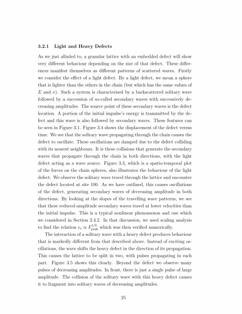
The interaction of a solitary wave with a heavy defect produces behaviour
that is markedly different from that described above. Instead of exciting os-
cillations, the wave shifts the heavy defect in the direction of its propagation.
This causes the lattice to be split in two, with pulses propagating in each
part. Figure 3.5 shows this clearly. Beyond the defect we observe many
pulses of decreasing amplitudes. In front, there is just a single pulse of large
amplitude. The collision of the solitary wave with this heavy defect causes
it to fragment into solitary waves of decreasing amplitudes.
25
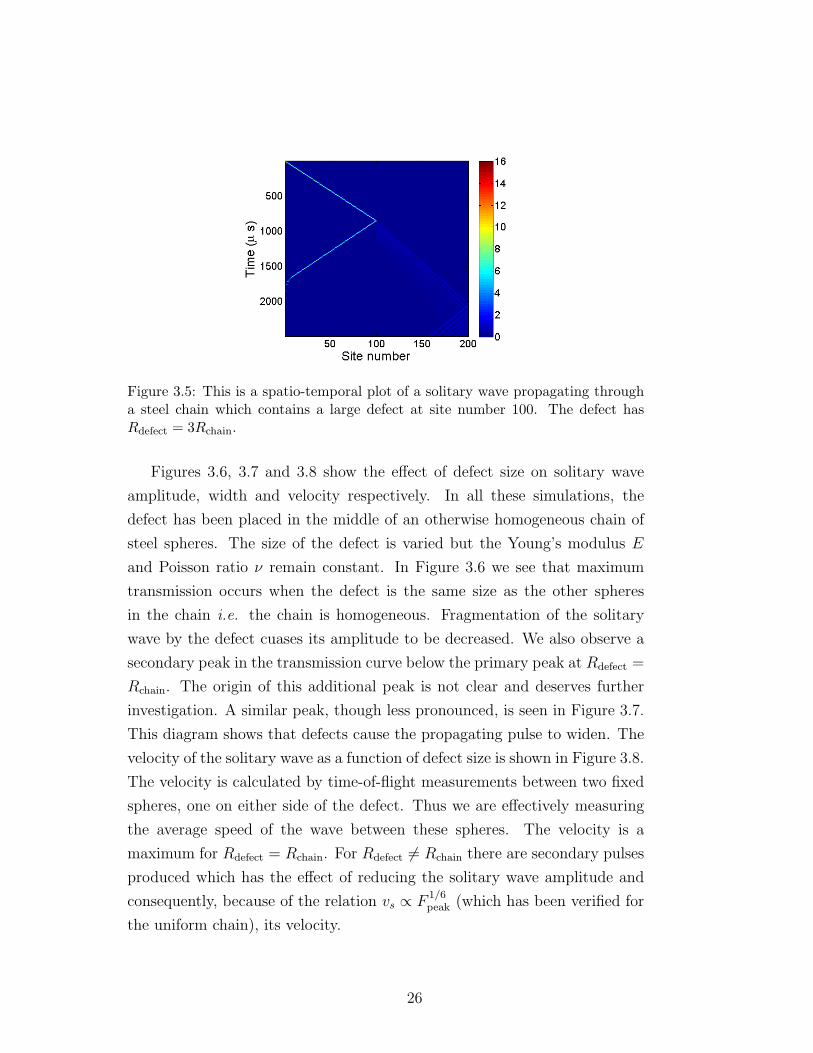
Figure 3.5: This is a spatio-temporal plot of a solitary wave propagating througha steel chain which contains a large defect at site number 100. The defect hasRdefect = 3Rchain.
Figures 3.6, 3.7 and 3.8 show the effect of defect size on solitary wave
amplitude, width and velocity respectively. In all these simulations, the
defect has been placed in the middle of an otherwise homogeneous chain of
steel spheres. The size of the defect is varied but the Young’s modulus E
and Poisson ratio ν remain constant. In Figure 3.6 we see that maximum
transmission occurs when the defect is the same size as the other spheres
in the chain i.e. the chain is homogeneous. Fragmentation of the solitary
wave by the defect cuases its amplitude to be decreased. We also observe a
secondary peak in the transmission curve below the primary peak at Rdefect =
Rchain. The origin of this additional peak is not clear and deserves further
investigation. A similar peak, though less pronounced, is seen in Figure 3.7.
This diagram shows that defects cause the propagating pulse to widen. The
velocity of the solitary wave as a function of defect size is shown in Figure 3.8.
The velocity is calculated by time-of-flight measurements between two fixed
spheres, one on either side of the defect. Thus we are effectively measuring
the average speed of the wave between these spheres. The velocity is a
maximum for Rdefect = Rchain. For Rdefect 6= Rchain there are secondary pulses
produced which has the effect of reducing the solitary wave amplitude and
consequently, because of the relation vs ∝ F1/6peak (which has been verified for
the uniform chain), its velocity.
26
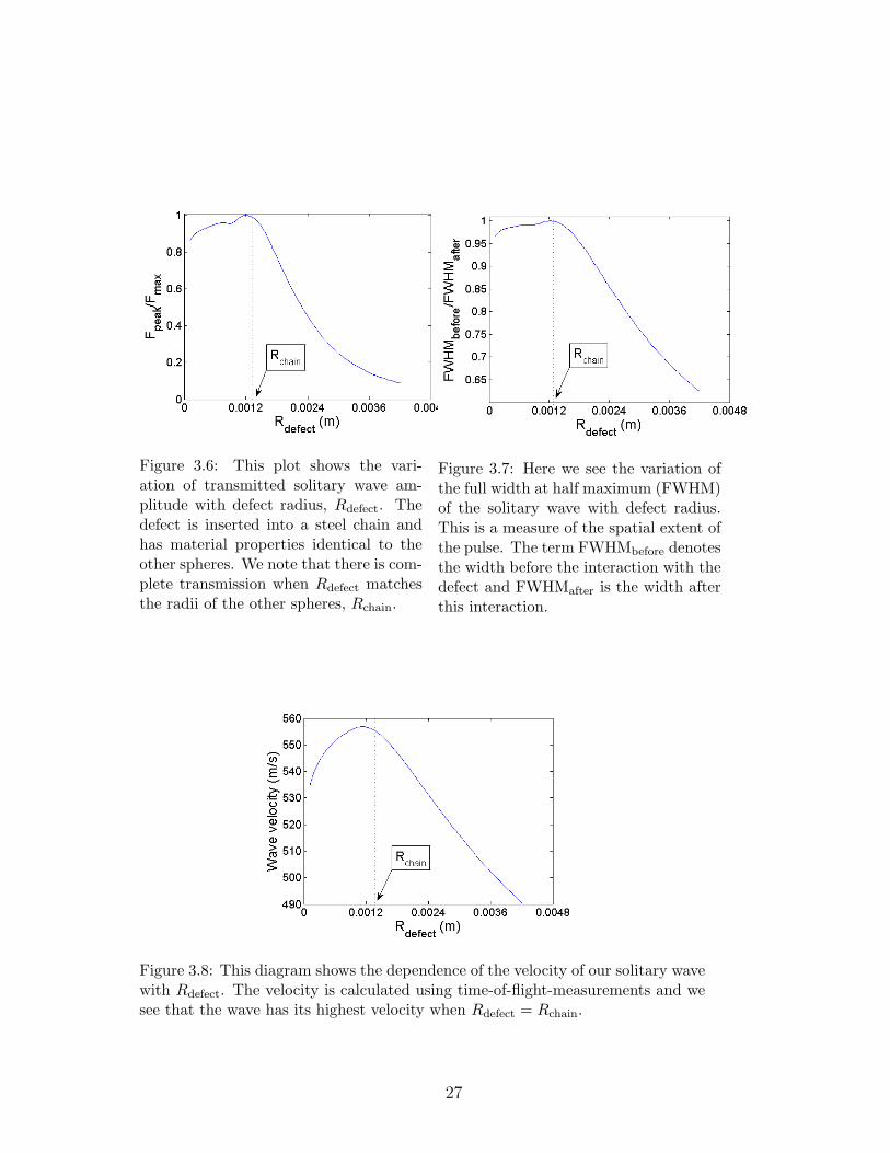
Figure 3.6: This plot shows the vari-ation of transmitted solitary wave am-plitude with defect radius, Rdefect. Thedefect is inserted into a steel chain andhas material properties identical to theother spheres. We note that there is com-plete transmission when Rdefect matchesthe radii of the other spheres, Rchain.
Figure 3.7: Here we see the variation ofthe full width at half maximum (FWHM)of the solitary wave with defect radius.This is a measure of the spatial extent ofthe pulse. The term FWHMbefore denotesthe width before the interaction with thedefect and FWHMafter is the width afterthis interaction.
Figure 3.8: This diagram shows the dependence of the velocity of our solitary wavewith Rdefect. The velocity is calculated using time-of-flight-measurements and wesee that the wave has its highest velocity when Rdefect = Rchain.
27
Figure 3.9: The variation of Fpeak/Fmax
with Young’s modulus E is plotted above.The size and other properties of the de-fect are kept constant and equal those ofthe other spheres.
Figure 3.10: This time we vary the Pois-son ratio ν and measure the transmittedamplitude of the incoming solitary wave.We again note that transmission is max-imised for νdefect = νchain.
3.2.2 The Effect of Young’s Modulus E and Poisson Ratio ν
In the previous section we considered a defect to be a sphere of varying size,
with all its other properties matching those of the chain. Now we consider
the effect of holding the defect size constant and varying, in turn, the Young’s
modulus E and Poisson ratio ν. The results are plotted in Figures 3.9-3.14.
In Figures 3.9 and 3.10 the transmitted solitary wave amplitude is plotted
as a function of E and ν respectively. Due to a material defect, the energy of
the solitary wave is not conserved as it moves through the granular lattice.
The interaction of the wave with the defect produces secondary waves that
carry away some of the original solitary wave’s energy [24]. It also causes the
amplitude of the wave to be decreased, as seen in Figures 3.9 and 3.10. The
variations are much smaller than those observed in Figure 3.6 indicating that
the defect’s mass is the predominant property when considering transmission.
The width of our solitary wave is measured both before and after inter-
action with the defect. The ratio FWHMbefore/FWHMafter is calculated for
varying E and ν. We observe that the pulse broadens as these properties
deviate from those of the other spheres in the chain.
Figures 3.13 and 3.14 show the variation of the wave velocity with E and
ν respectively. As the defect becomes “stiffer”, i.e. as E increases, the speed
28
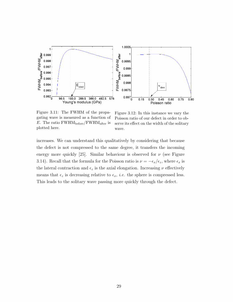
Figure 3.11: The FWHM of the propa-gating wave is measured as a function ofE. The ratio FWHMbefore/FWHMafter isplotted here.
Figure 3.12: In this instance we vary thePoisson ratio of our defect in order to ob-serve its effect on the width of the solitarywave.
increases. We can understand this qualitatively by considering that because
the defect is not compressed to the same degree, it transfers the incoming
energy more quickly [25]. Similar behaviour is observed for ν (see Figure
3.14). Recall that the formula for the Poisson ratio is ν = −εx/εz, where εx is
the lateral contraction and εz is the axial elongation. Increasing ν effectively
means that εz is decreasing relative to εx, i.e. the sphere is compressed less.
This leads to the solitary wave passing more quickly through the defect.
29
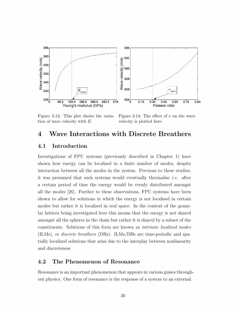
Figure 3.13: This plot shows the varia-tion of wave velocity with E.
Figure 3.14: The effect of ν on the wavevelocity is plotted here.
4 Wave Interactions with Discrete Breathers
4.1 Introduction
Investigations of FPU systems (previously described in Chapter 1) have
shown how energy can be localised in a finite number of modes, despite
interaction between all the modes in the system. Previous to these studies,
it was presumed that such systems would eventually thermalise i.e. after
a certain period of time the energy would be evenly distributed amongst
all the modes [26]. Further to these observations, FPU systems have been
shown to allow for solutions in which the energy is not localised in certain
modes but rather it is localised in real space. In the context of the granu-
lar lattices being investigated here this means that the energy is not shared
amongst all the spheres in the chain but rather it is shared by a subset of the
constituents. Solutions of this form are known as intrinsic localised modes
(ILMs), or discrete breathers (DBs). ILMs/DBs are time-periodic and spa-
tially localized solutions that arise due to the interplay between nonlinearity
and discreteness
4.2 The Phenomenon of Resonance
Resonance is an important phenomenon that appears in various guises through-
out physics. One form of resonance is the response of a system to an external
30
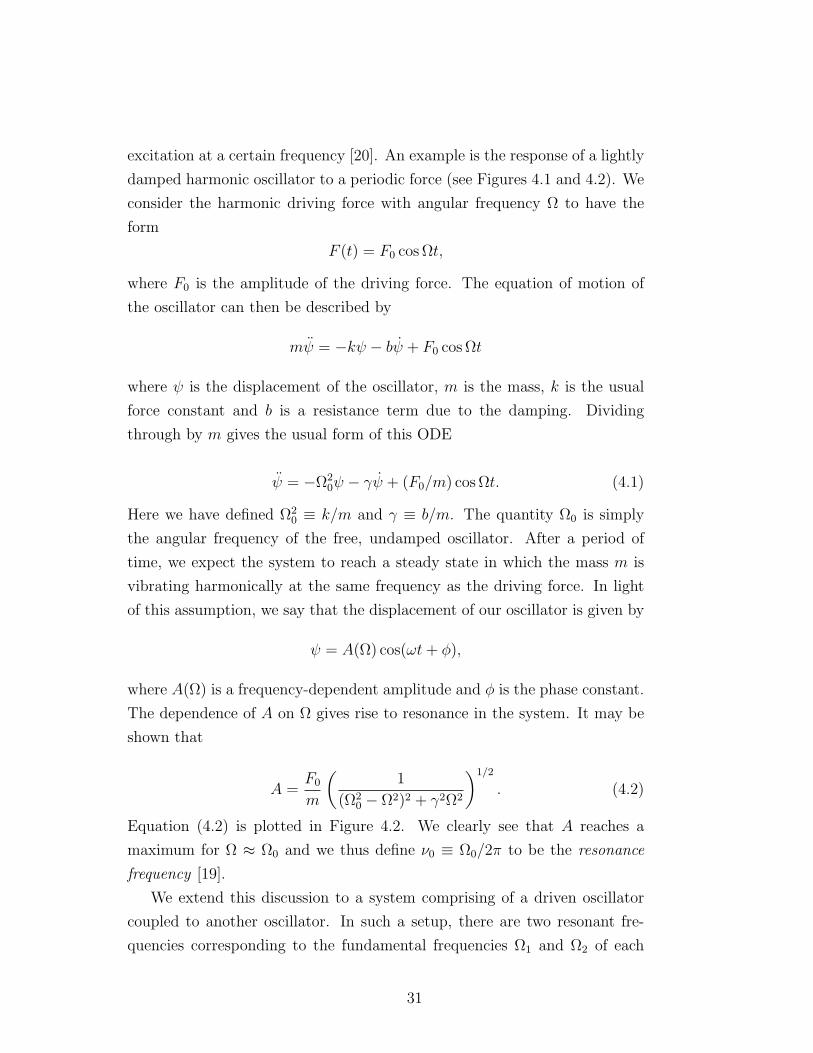
excitation at a certain frequency [20]. An example is the response of a lightly
damped harmonic oscillator to a periodic force (see Figures 4.1 and 4.2). We
consider the harmonic driving force with angular frequency Ω to have the
form
F (t) = F0 cos Ωt,
where F0 is the amplitude of the driving force. The equation of motion of
the oscillator can then be described by
mψ = −kψ − bψ + F0 cos Ωt
where ψ is the displacement of the oscillator, m is the mass, k is the usual
force constant and b is a resistance term due to the damping. Dividing
through by m gives the usual form of this ODE
ψ = −Ω20ψ − γψ + (F0/m) cos Ωt. (4.1)
Here we have defined Ω20 ≡ k/m and γ ≡ b/m. The quantity Ω0 is simply
the angular frequency of the free, undamped oscillator. After a period of
time, we expect the system to reach a steady state in which the mass m is
vibrating harmonically at the same frequency as the driving force. In light
of this assumption, we say that the displacement of our oscillator is given by
ψ = A(Ω) cos(ωt+ φ),
where A(Ω) is a frequency-dependent amplitude and φ is the phase constant.
The dependence of A on Ω gives rise to resonance in the system. It may be
shown that
A =F0
m
(1
(Ω20 − Ω2)2 + γ2Ω2
)1/2
. (4.2)
Equation (4.2) is plotted in Figure 4.2. We clearly see that A reaches a
maximum for Ω ≈ Ω0 and we thus define ν0 ≡ Ω0/2π to be the resonance
frequency [19].
We extend this discussion to a system comprising of a driven oscillator
coupled to another oscillator. In such a setup, there are two resonant fre-
quencies corresponding to the fundamental frequencies Ω1 and Ω2 of each
31
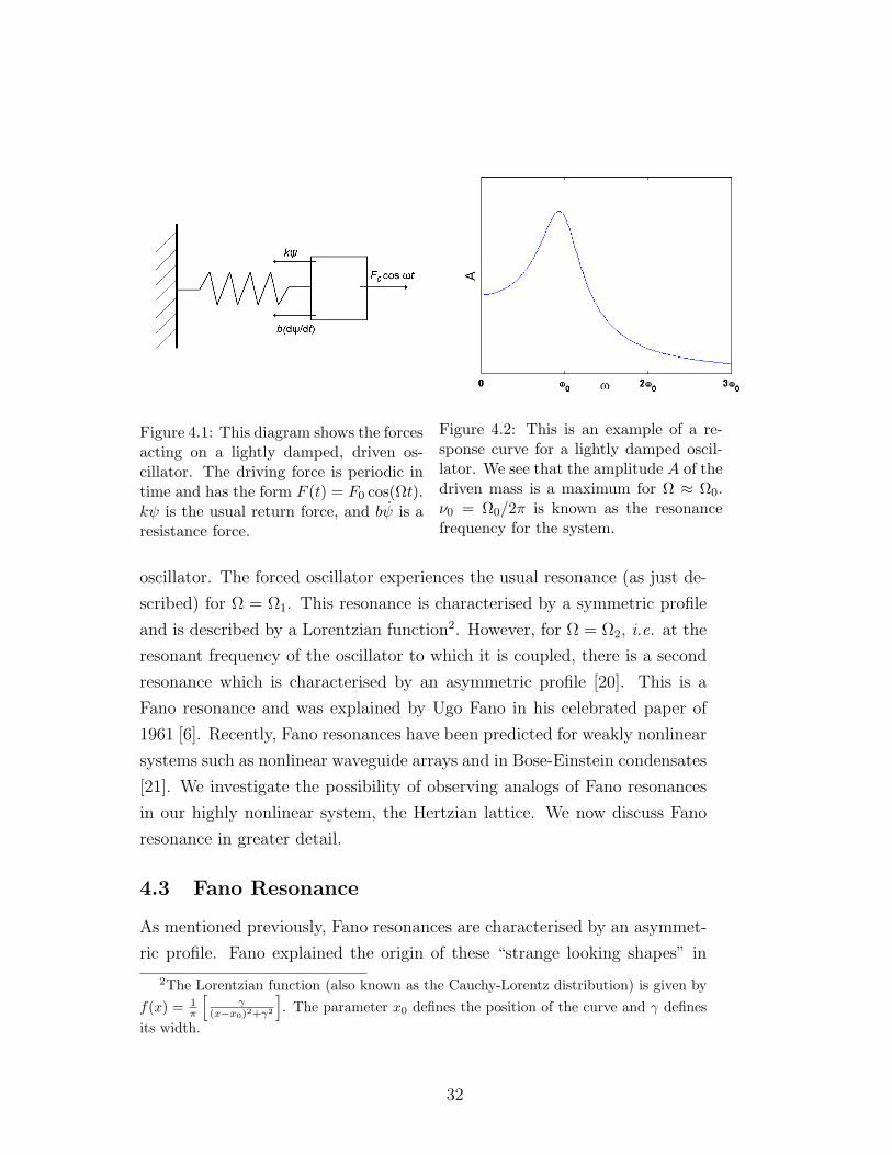
Figure 4.1: This diagram shows the forcesacting on a lightly damped, driven os-cillator. The driving force is periodic intime and has the form F (t) = F0 cos(Ωt).kψ is the usual return force, and bψ is aresistance force.
Figure 4.2: This is an example of a re-sponse curve for a lightly damped oscil-lator. We see that the amplitude A of thedriven mass is a maximum for Ω ≈ Ω0.ν0 = Ω0/2π is known as the resonancefrequency for the system.
oscillator. The forced oscillator experiences the usual resonance (as just de-
scribed) for Ω = Ω1. This resonance is characterised by a symmetric profile
and is described by a Lorentzian function2. However, for Ω = Ω2, i.e. at the
resonant frequency of the oscillator to which it is coupled, there is a second
resonance which is characterised by an asymmetric profile [20]. This is a
Fano resonance and was explained by Ugo Fano in his celebrated paper of
1961 [6]. Recently, Fano resonances have been predicted for weakly nonlinear
systems such as nonlinear waveguide arrays and in Bose-Einstein condensates
[21]. We investigate the possibility of observing analogs of Fano resonances
in our highly nonlinear system, the Hertzian lattice. We now discuss Fano
resonance in greater detail.
4.3 Fano Resonance
As mentioned previously, Fano resonances are characterised by an asymmet-
ric profile. Fano explained the origin of these “strange looking shapes” in
2The Lorentzian function (also known as the Cauchy-Lorentz distribution) is given byf(x) = 1
π
[γ
(x−x0)2+γ2
]. The parameter x0 defines the position of the curve and γ defines
its width.
32
terms of the interaction of a localised state with a continuum of propagation
modes. His description was initially introduced to explain sharp, asymmet-
ric profiles in atomic absorption spectra which had been observed by Beutler
[20]. Fano hypothesised that the unexpected profiles arose due to the inter-
action of a discrete excited state of an atom with a continuum which shared
the same energy. The interaction results in interference and the observed
profiles.
A qualitative understanding of these novel resonances was provided by
Fano in terms of the absorption of radiation by atoms. We now present
an account of this explanation based on the description given in Ref. [20].
Quantum theory tells us that electrons in atoms may only have certain energy
values i.e. the energy spectrum is discrete rather than continuous. Electrons
may move between different energy levels by absorbing or emitting packets
of radiation called photons. The energy of a photon is given by Ephoton = ~ω.
If Ephoton = E2 − E1, where E1 and E2 are the energies of levels 1 and 2
respectively, then an electron may move between these levels by absorbing
or emitting a photon of this frequency. Thus if we shine light of varying
frequency on a sample of atoms, there will be absorption resonance curves
at values of ω corresponding to various energy gaps. These absorption peaks
are symmetric and may be represented using the Lorentzian function defined
in the previous section.
However, a different situation can arise whereby absorption of radiation
occurs via a different mechanism. The Auger effect describes how an electron
from the inner core of an atom can be removed by high energy radiation (such
as an X-ray) leaving a vacancy in the core. An electron from a higher energy
level may relax into this “electron hole” resulting in a release of energy.
Sometimes this energy can be emitted in the form of a photon but often it is
transferred to another electron which is above the ionisation threshold and
this electron will escape from the atom. Due to the superposition principle,
the Auger effect can interfere with the normal relaxation processes in an
atom and this manifests itself as an asymmetric peak in the spectra of that
atom (Fano resonance).
An important concept in the understanding of Fano resonance (and of
wave scattering in general) is that of “channels”. In an atom, an excited
33
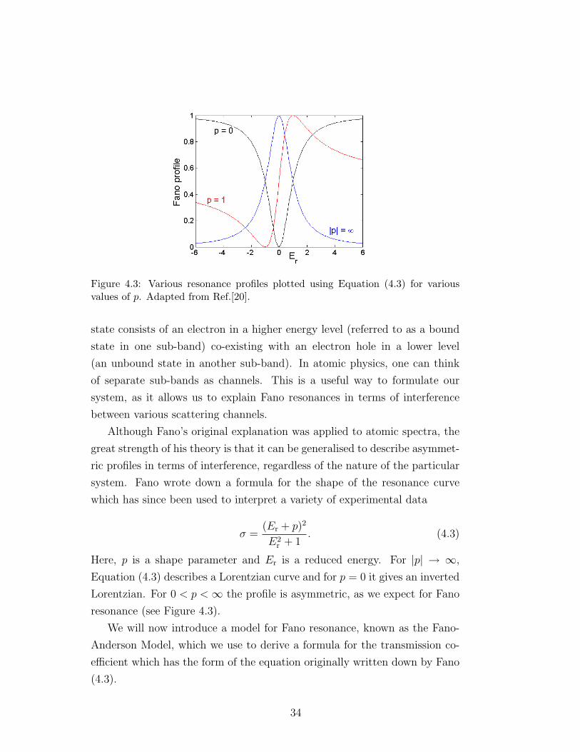
Figure 4.3: Various resonance profiles plotted using Equation (4.3) for variousvalues of p. Adapted from Ref.[20].
state consists of an electron in a higher energy level (referred to as a bound
state in one sub-band) co-existing with an electron hole in a lower level
(an unbound state in another sub-band). In atomic physics, one can think
of separate sub-bands as channels. This is a useful way to formulate our
system, as it allows us to explain Fano resonances in terms of interference
between various scattering channels.
Although Fano’s original explanation was applied to atomic spectra, the
great strength of his theory is that it can be generalised to describe asymmet-
ric profiles in terms of interference, regardless of the nature of the particular
system. Fano wrote down a formula for the shape of the resonance curve
which has since been used to interpret a variety of experimental data
σ =(Er + p)2
E2r + 1
. (4.3)
Here, p is a shape parameter and Er is a reduced energy. For |p| → ∞,
Equation (4.3) describes a Lorentzian curve and for p = 0 it gives an inverted
Lorentzian. For 0 < p <∞ the profile is asymmetric, as we expect for Fano
resonance (see Figure 4.3).
We will now introduce a model for Fano resonance, known as the Fano-
Anderson Model, which we use to derive a formula for the transmission co-
efficient which has the form of the equation originally written down by Fano
(4.3).
34
4.3.1 The Fano-Anderson Model
A relatively simple model that can be often invoked to explain the physics of
Fano resonance is the Fano-Anderson model. This is a discrete model which
can be described by the following Hamiltonian [20]
H =∑n
Cφnφ∗n−1 + EF |ψ|2 + VFψ
∗φ0 + complex conjugates, (4.4)
where the asterisk denotes the complex conjugate and H describes the energy
of two subsystems. The first is a linear discrete chain with field amplitude φn
at site n. The symbol C denotes the coupling constant between neighbouring
sites. This system allows the propagation of plane waves with the dispersion
relation ωq = 2C cos q. The state of the second subsystem is denoted ψ and
has an energy value EF , where EF denotes the Fermi energy. The interaction
between the subsystems is described by the coupling term VF from the state
ψ to site 0 of the discrete chain, φ0. Using Equation (4.4) the following
dynamical equations can be obtained:
iφn = C(φn−1 + φn+1) + VFψδn0
iψ = EFψ + VFφ0
(4.5)
where δn0 denotes the Kronecker delta. Due to the gauge invariance of these
equation, the time dependence can be removed using the ansatz
φn(t) = Ane−iωt,
ψn(t) = Be−iωt.(4.6)
These expressions inserted into Equations (4.5) give the following static equa-
tions
ωAn = C(An−1 + An+1) + VFBδn0,
ωB = EFB + VFA0.(4.7)
Given the dispersion relation for the linear system, i.e. ωq = 2C cos q, we
should look to solve the above system of equations using frequencies from
35
the propagation band i.e. ω = ωq. We are dealing with a wave scattering
problem so we can impose the following boundary conditions on An:
An =
IFanoeiqn + rFanoe−iqn, n < 0TFanoeiqn, n > 0
(4.8)
where IFano, rFano and TFano are the incoming, reflected and transmitted wave
amplitudes respectively. We use the second equation in the system (4.7) to
obtain
B =VFA0
ωq − EF.
Our system (4.7) can now be reduced to
ωqAn = C(An−1 + An+1) +V 2F
ωq − EFA0δn0. (4.9)
Examining Equation (4.9), we see that the magnitude of the scattering po-
tential V 2F /(ωq − EF ) is dependent on the plane wave frequency ωq. This is
important, as we note that for ωq = EF , the scattering potential is infinite
and prevents transmission of the incoming wave. This is a key feature of
Fano resonance.
We can derive an expression for the transmission coefficient T = |TFano/IFano|2
using a transfer matrix approach as described in Ref.[29]. First, write Equa-
tion (4.9) in the form of a transfer matrix
C
(An+1
An/C
)= Tn
(AnAn−1
)(4.10)
with
Tn =
(ωq −
V 2F
ωq−EFδn0 −C
1 0
). (4.11)
If there are n = Nleft sites to the left of site n = 0 and n = Nright sites to
the right, then we can write
C
(ANright
ANright−1/C
)= PNright
(A−Nleft+1
A−Nleft
)(4.12)
where
36
PNright= TNright
TNright−1 · · ·T1T0T−1 · · ·T−Nleft.
Using Equations (4.8) and (4.12) an expression for T may be derived. This
is given in Ref.[20] as
T =α2q
α2q + 1
, (4.13)
where
αq = cq(EF − ωq)/V 2F , cq = 2C sin q.
We note that Equation 4.13 corresponds to the formula introduced by Fano
(Equation (4.3)) to explain the unusual atomic absorption lines observed by
Beutler. Transmission vanishes for ωq = EF .
These discussions have shown the possibility of waves travelling through
a the linear chain interacting with those in the discrete state leading to Fano
resonance.
4.4 Discrete Breathers
As we have discussed in previous chapters, nonlinear lattices can support the
propagation of weakly and strongly nonlinear waves. These are solutions to
the equations of motion of the system, which are characterised by Hertzian
interactions between neighbouring spheres. Another family of solutions are
DBs, which are spatially localised and often time periodic excitations of the
lattice. In this chapter, we consider DBs in a precompressed chain. Snapshots
of an oscillating DB are shown in Figure 4.4. DBs are similar to solitary
waves with the added property of being periodic in time. They arise due
to the interplay of nonlinearity and discreteness in the system. Nonlinearity
indicates that the DB amplitude and localisation length are dependent on
the frequency of oscillation, Ωb, and can therefore be tuned. Discreteness
means that there is an upper bound, ωq, on the frequency spectrum of the
waves that can propagate through the chain [9].
The phenomenon of localised modes, and DBs in particular, is quite
widespread and such states have been experimentally observed in fields as
diverse as nonlinear optics, Josephson junctions, magnetic systems, and in
the lattice dynamics of crystals [9].
37
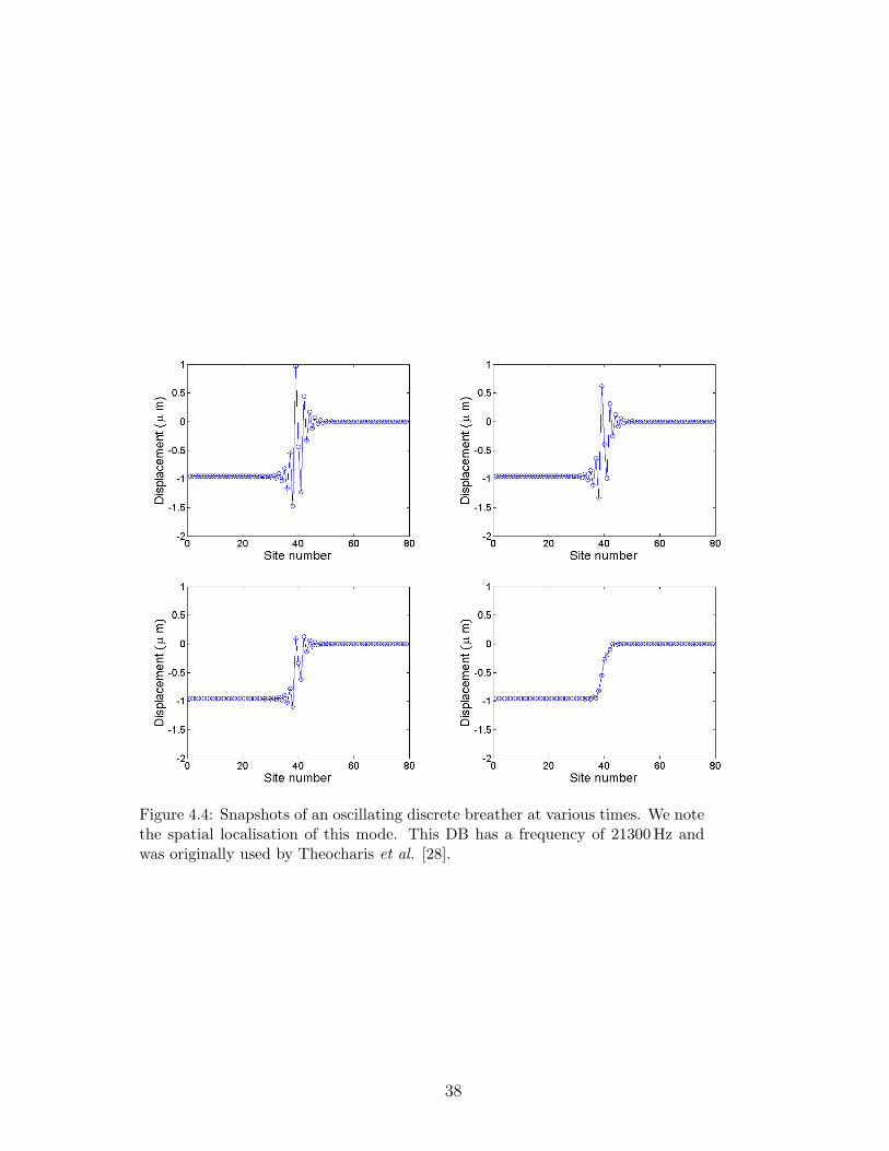
Figure 4.4: Snapshots of an oscillating discrete breather at various times. We notethe spatial localisation of this mode. This DB has a frequency of 21300 Hz andwas originally used by Theocharis et al. [28].
38
We begin a more quantitative description of DBs by considering the total
energy of our precompressed granular lattice i.e. the Hamiltonian H of the
system. The Hamiltonian will have kinetic energy (arising from the motion of
the spheres) and potential energy (due to sphere-sphere interactions) terms,
and we express it as
H =∑n
(1
2p2n +W (un − un−1)
). (4.14)
As in previous chapters, un denotes the displacement of sphere n from equi-
librium. The momentum is given by pn = un ≡ dun/dt and W (u) is the
interaction potential between spheres. The following conditions apply to
W (u); W (0) = W ′(0) = 0 and additionally we assume that W ′′ is positive
for small displacements, W ′′(0) > 0. The classical Hamilton equations of
motion are written as
un =∂H
∂pn, pn = − ∂H
∂un,
which lead us to a familiar set of coupled ODEs
un = −W ′(un − un−1) +W ′(un+1 − un). (4.15)
We expand W as a power series
W (u) =∞∑m
φmmum. (4.16)
Considering only small velocities and amplitudes, one can neglect all nonlin-
ear terms from the equations of motion and assume that φm = 0 for m > 2.
Thus, the coupled ODEs are now linear and have the form
un = φ2(un+1 + un−1 − 2un). (4.17)
The solution to this ODE can be written as a superposition of plane waves
where each is given by
un(t) = Aq cos(ωqt− qn+Bq), (4.18)
39
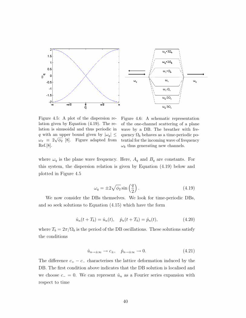
Figure 4.5: A plot of the dispersion re-lation given by Equation (4.19). The re-lation is sinusoidal and thus periodic inq with an upper bound given by |ωq| ≤ωπ ≡ 2
√φ2 [8]. Figure adapted from
Ref.[8].
Figure 4.6: A schematic representationof the one-channel scattering of a planewave by a DB. The breather with fre-quency Ωb behaves as a time-periodic po-tential for the incoming wave of frequencyωk thus generating new channels.
where ωq is the plane wave frequency. Here, Aq and Bq are constants. For
this system, the dispersion relation is given by Equation (4.19) below and
plotted in Figure 4.5
ωq = ±2√φ2 sin
(q2
). (4.19)
We now consider the DBs themselves. We look for time-periodic DBs,
and so seek solutions to Equation (4.15) which have the form
un(t+ Tb) = un(t), pn(t+ Tb) = pn(t), (4.20)
where Tb = 2π/Ωb is the period of the DB oscillations. These solutions satisfy
the conditions
un→±∞ → c±, pn→±∞ → 0. (4.21)
The difference c+ − c− characterises the lattice deformation induced by the
DB. The first condition above indicates that the DB solution is localised and
we choose c− = 0. We can represent un as a Fourier series expansion with
respect to time
40
un(t) =+∞∑j=−∞
AjneikΩbt (4.22)
and the localisation condition given by Equation (4.21) becomes
Aj 6=0,n→±∞ → 0, Aj=0,n→±∞ → c±. (4.23)
Substituting Equation (4.22) into the original system (4.15), a linearisation
of the expressions for Ajn and the boundary conditions (4.23) leads to the
nonresonance condition
jΩb 6= ωq (4.24)
for all i. This condition implies that Ωb > ωq (excluding the case where
j = 0).
An important property of localised modes is their stability, which can be
analysed by adding a small perturbation to the DB solution un:
un(t) = un + εn(t)
Inserting this expression into Equation (4.15), and retaining only the terms
that are linear in εn, we obtain the first order ODE system
εn = −W ′′(un − un−1)(εn − εn−1) +W ′′(un+1 − n)(εn+1 − εn). (4.25)
Integration of these equations relate ε(t) and ε(t) at t = Tb to the initial
conditions at t = 0 [4]. It also defines the following map(ε(Tb)ε(Tb)
)= F
(ε(0)ε(0)
)(4.26)
where we have defined ε ≡ (ε1, ε2, . . . ) and F is a symplectic Floquet ma-
trix. In general,a symplectic matrix A is a square matrix which satisfies
ATΓA = Γ, where Γ is a nonsingular, skew-symmetric matrix. Floquet the-
ory relates to ODEs which have the form x = B(t)x, where B(t) is a periodic
function. For a detailed discussion of Floquet matrices in the context of DBs
see Section VIII.A of Ref.[11]. The eigenvalues λ and eigenvectors ~y of F
41
provide information on the stability. A DB is said to be linearly stable if all
of the eigenvalues of its Floquet matrix F lie on the unit circle. This means
that any small perturbation to the system will not grow exponentially with
time [4]. In this case, the eigenvalues can be written as eiθ. The eigenvectors
are solutions to the Equation (4.25) and satisfy the Bloch condition [16]
εn(t+ Tb) = e−iθεn(t) (4.27)
where θ = ±ωqTb are the Floquet phases [10]. Using the Bloch condition, we
may now write solutions of Equation (4.25) in the form
εn(t) =+∞∑j=−∞
εnjei(ωq+jΩb)t. (4.28)
In Section 4.2 we introduced the idea of channels. The DB acts as a
time-periodic scattering potential for the incoming wave of frequency ωq and
as such, generates new channels of propagation at frequencies ωq + jΩb. If
ωq + jΩb 6= ωq′ for nonzero j then all channels are “closed” except for the
“open” channel j = 0. This situation corresponds to elastic scattering i.e.
the energies of the transmitted and reflected waves are equal. Otherwise, the
scattering is inelastic [8]. These channels are shown schematically in Figure
4.6.
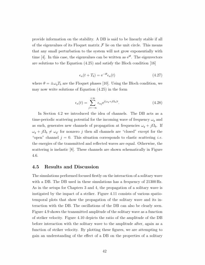
4.5 Results and Discussion
The simulations performed focused firstly on the interaction of a solitary wave
with a DB. The DB used in these simulations has a frequency of 21300 Hz.
As in the setups for Chapters 3 and 4, the propagation of a solitary wave is
instigated by the impact of a striker. Figure 4.11 consists of various spatio-
temporal plots that show the propagation of the solitary wave and its in-
teraction with the DB. The oscillations of the DB can also be clearly seen.
Figure 4.9 shows the transmitted amplitude of the solitary wave as a function
of striker velocity. Figure 4.10 depicts the ratio of the amplitude of the DB
before interaction with the solitary wave to the amplitude after, again as a
function of striker velocity. By plotting these figures, we are attempting to
gain an understanding of the effect of a DB on the properties of a solitary
42
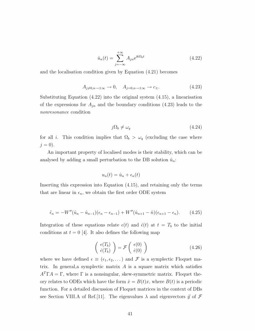
Figure 4.7: The other scenario we studyis the interaction of an impulse, gener-ated by a striker, with a DB.
Figure 4.8: This diagram shows the ini-tial setup of our simulation to investigatea plane wave’s interaction with a DB.
Figure 4.9: The transmitted amplitude ofthe solitary wave as a function of strikervelocity. Fmax is the initial amplitudeand Fpeak the amplitude after interactionwith the DB.
Figure 4.10: The ratio of the maximumamplitude of the DB before interactionwith the solitary wave to the maximumamplitude after, as a function of strikervelocity.
43
wave, and vice versa. Further research in this area is needed, perhaps using
additional DBs and solitary waves of different widths and amplitudes.
Finally, we examine the interaction of an attenuated plane wave with the
DB. Our goal is to create a plot analogous to Figure 3 of Ref. [21], which
shows the transmission coefficient of a plane wave interacting with a nonlinear
impurity mode as a function of wavenumber q. This figure shows the pos-
sibility of observing Fano resonances in saturable waveguide arrays. We are
interesting in investigating whether a nonlinear analogy of Fano resonance
can be observed in our system. Figure 4.8 shows an incoming attenuated
plane wave and the DB. The transmitted amplitude as a function of q is
given in Figure 4.12. Although there appear to be certain resonances in the
system, there is not a direct correspondence between these results and those
presented in Figure 3 of Ref. [21]. Consequently, we are unable to confirm
whether Fano resonances are possible in this granular system. Further stud-
ies will be necessary to investigate this system in greater detail in an effort
to explain the features of Figure 4.12.
44
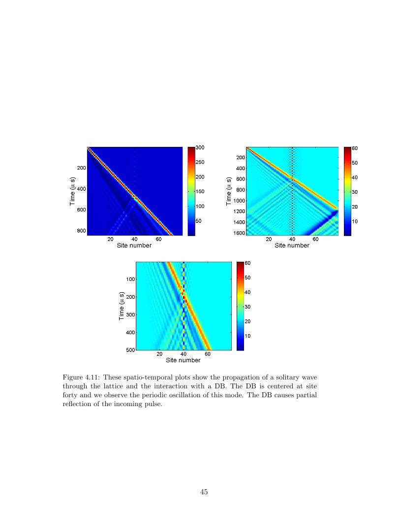
Figure 4.11: These spatio-temporal plots show the propagation of a solitary wavethrough the lattice and the interaction with a DB. The DB is centered at siteforty and we observe the periodic oscillation of this mode. The DB causes partialreflection of the incoming pulse.
45
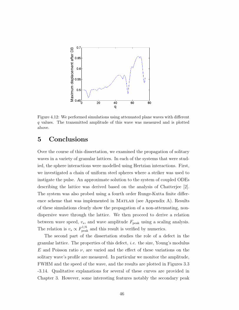
Figure 4.12: We performed simulations using attenuated plane waves with differentq values. The transmitted amplitude of this wave was measured and is plottedabove.
5 Conclusions
Over the course of this dissertation, we examined the propagation of solitary
waves in a variety of granular lattices. In each of the systems that were stud-
ied, the sphere interactions were modelled using Hertzian interactions. First,
we investigated a chain of uniform steel spheres where a striker was used to
instigate the pulse. An approximate solution to the system of coupled ODEs
describing the lattice was derived based on the analysis of Chatterjee [2].
The system was also probed using a fourth order Runge-Kutta finite differ-
ence scheme that was implemented in Matlab (see Appendix A). Results
of these simulations clearly show the propagation of a non-attenuating, non-
dispersive wave through the lattice. We then proceed to derive a relation
between wave speed, vs, and wave amplitude Fpeak using a scaling analysis.
The relation is vs ∝ F1/6peak and this result is verified by numerics.
The second part of the dissertation studies the role of a defect in the
granular lattice. The properties of this defect, i.e. the size, Young’s modulus
E and Poisson ratio ν, are varied and the effect of these variations on the
solitary wave’s profile are measured. In particular we monitor the amplitude,
FWHM and the speed of the wave, and the results are plotted in Figures 3.3
-3.14. Qualitative explanations for several of these curves are provided in
Chapter 3. However, some interesting features notably the secondary peak
46
observed in Figure 3.6 (and to a lesser extent in Figure 3.7) are not clearly
understood. A qualitative and quantitative description of these diagrams
should be a goal of future work in this area.
In Chapter 4 we introduced the concept of localised modes, specifically
DBs. The scattering of plane waves off DBs has been shown to produce
interesting resonance phenomena. Work by Naether et al. on waveguide
arrays had shown that Fano resonance could be observed in these systems
[21]. Using this work as a reference, we investigated whether our granular
lattice would show similar results. We employed the same numerical setup
as that used by Theocharis et al. [28] in which a DB is established in the
middle of a precompressed chain. We scatter plane waves with varying q off
the DB and measure the transmitted amplitude (see Figure 4.12). However,
there is not a direct correspondence between these results and those produced
by Naether et al.. Nevertheless, there appear to be interesting features in
Figure 4.12 that we don’t yet understand physically and this will be a focus
of future work.
47
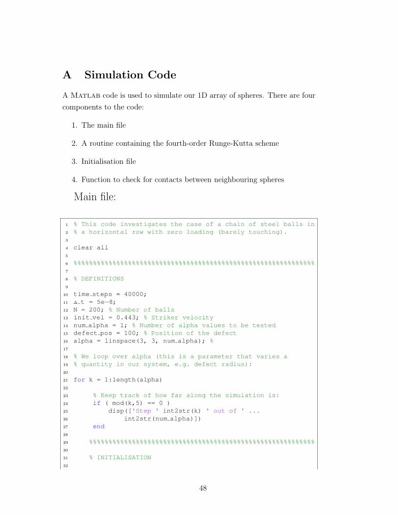
A Simulation Code
A Matlab code is used to simulate our 1D array of spheres. There are four
components to the code:
1. The main file
2. A routine containing the fourth-order Runge-Kutta scheme
3. Initialisation file
4. Function to check for contacts between neighbouring spheres
Main file:
1 % This code investigates the case of a chain of steel balls in2 % a horizontal row with zero loading (barely touching).3
4 clear all5
6 %%%%%%%%%%%%%%%%%%%%%%%%%%%%%%%%%%%%%%%%%%%%%%%%%%%%%%%%%%%%%%7
8 % DEFINITIONS9
10 time steps = 40000;11 ∆ t = 5e−8;12 N = 200; % Number of balls13 init vel = 0.443; % Striker velocity14 num alpha = 1; % Number of alpha values to be tested15 defect pos = 100; % Position of the defect16 alpha = linspace(3, 3, num alpha); %17
18 % We loop over alpha (this is a parameter that varies a19 % quantity in our system, e.g. defect radius):20
21 for k = 1:length(alpha)22
23 % Keep track of how far along the simulation is:24 if ( mod(k,5) == 0 )25 disp(['Step ' int2str(k) ' out of ' ...26 int2str(num alpha)])27 end28
29 %%%%%%%%%%%%%%%%%%%%%%%%%%%%%%%%%%%%%%%%%%%%%%%%%%%%%%%%%%30
31 % INITIALISATION32
48
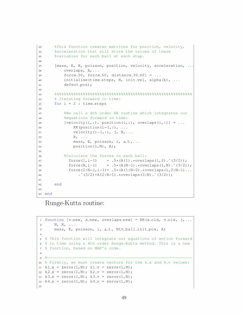
33 %This function creates matrices for position, velocity,34 %acceleration that will store the values of these35 %variables for each ball at each step.36
37 [mass, E, R, poisson, position, velocity, acceleration, ...38 overlaps, A,...39 force 30, force 60, distance 30 60] = ...40 initialise(time steps, N, init vel, alpha(k), ...41 defect pos);42
43 %%%%%%%%%%%%%%%%%%%%%%%%%%%%%%%%%%%%%%%%%%%%%%%%%%%%%%%%%%44 % Iterating forward in time:45 for i = 2 : time steps46
47 %We call a 4th order RK routine which integrates our48 %equations forward in time:49 [velocity(i,:), position(i,:), overlaps(i,:)] = ...50 RK(position(i−1,:), ...51 velocity(i−1,:), j, N,...52 R, ...53 mass, E, poisson, i, ∆ t,...54 position(1,N), A);55
56 %Calculate the forces on each ball:57 force(1,i−1) = .5*(A(1).*overlaps(i,2).ˆ(3/2));58 force(N,i−1) = .5*(A(N−1).*overlaps(i,N).ˆ(3/2));59 force(2:N−1,i−1)= .5*(A(1:N−2).*overlaps(i,2:N−1)...60 .ˆ(3/2)+A(2:N−1).*overlaps(3:N).ˆ(3/2));61
62 end63
64 end
Runge-Kutta routine:
1 function [v new, x new, overlaps new] = RK(x old, v old, j,...2 N, R, ...3 mass, E, poisson, i, ∆ t, Nth ball init pos, A)4
5 % This function will integrate our equations of motion forward6 % in time using a 4th order Runge−Kutta method. This is a new7 % function, based on MAP's code.8
9 %−−−−−−−−−−−−−−−−−−−−−−−−−−−−−−−−−−−−−−−−−−−−−−−−−−−−−−−−−−−−−10 % Firstly, we must create vectors for the k x and k v values:11 k1 x = zeros(1,N); k1 v = zeros(1,N);12 k2 x = zeros(1,N); k2 v = zeros(1,N);13 k3 x = zeros(1,N); k3 v = zeros(1,N);14 k4 x = zeros(1,N); k4 v = zeros(1,N);15
49
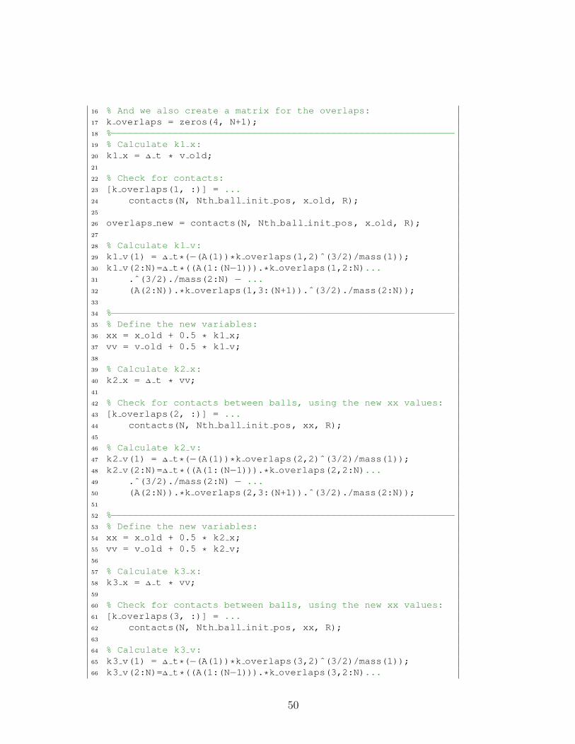
16 % And we also create a matrix for the overlaps:17 k overlaps = zeros(4, N+1);18 %−−−−−−−−−−−−−−−−−−−−−−−−−−−−−−−−−−−−−−−−−−−−−−−−−−−−−−−−−−−−−19 % Calculate k1 x:20 k1 x = ∆ t * v old;21
22 % Check for contacts:23 [k overlaps(1, :)] = ...24 contacts(N, Nth ball init pos, x old, R);25
26 overlaps new = contacts(N, Nth ball init pos, x old, R);27
28 % Calculate k1 v:29 k1 v(1) = ∆ t*(−(A(1))*k overlaps(1,2)ˆ(3/2)/mass(1));30 k1 v(2:N)=∆ t*((A(1:(N−1))).*k overlaps(1,2:N)...31 .ˆ(3/2)./mass(2:N) − ...32 (A(2:N)).*k overlaps(1,3:(N+1)).ˆ(3/2)./mass(2:N));33
34 %−−−−−−−−−−−−−−−−−−−−−−−−−−−−−−−−−−−−−−−−−−−−−−−−−−−−−−−−−−−−−35 % Define the new variables:36 xx = x old + 0.5 * k1 x;37 vv = v old + 0.5 * k1 v;38
39 % Calculate k2 x:40 k2 x = ∆ t * vv;41
42 % Check for contacts between balls, using the new xx values:43 [k overlaps(2, :)] = ...44 contacts(N, Nth ball init pos, xx, R);45
46 % Calculate k2 v:47 k2 v(1) = ∆ t*(−(A(1))*k overlaps(2,2)ˆ(3/2)/mass(1));48 k2 v(2:N)=∆ t*((A(1:(N−1))).*k overlaps(2,2:N)...49 .ˆ(3/2)./mass(2:N) − ...50 (A(2:N)).*k overlaps(2,3:(N+1)).ˆ(3/2)./mass(2:N));51
52 %−−−−−−−−−−−−−−−−−−−−−−−−−−−−−−−−−−−−−−−−−−−−−−−−−−−−−−−−−−−−−53 % Define the new variables:54 xx = x old + 0.5 * k2 x;55 vv = v old + 0.5 * k2 v;56
57 % Calculate k3 x:58 k3 x = ∆ t * vv;59
60 % Check for contacts between balls, using the new xx values:61 [k overlaps(3, :)] = ...62 contacts(N, Nth ball init pos, xx, R);63
64 % Calculate k3 v:65 k3 v(1) = ∆ t*(−(A(1))*k overlaps(3,2)ˆ(3/2)/mass(1));66 k3 v(2:N)=∆ t*((A(1:(N−1))).*k overlaps(3,2:N)...
50
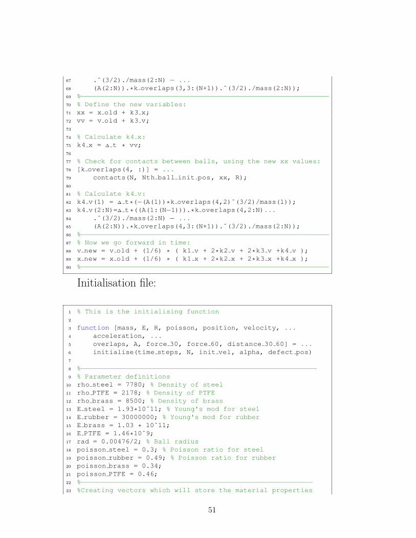
67 .ˆ(3/2)./mass(2:N) − ...68 (A(2:N)).*k overlaps(3,3:(N+1)).ˆ(3/2)./mass(2:N));69 %−−−−−−−−−−−−−−−−−−−−−−−−−−−−−−−−−−−−−−−−−−−−−−−−−−−−−−−−−−−−−70 % Define the new variables:71 xx = x old + k3 x;72 vv = v old + k3 v;73
74 % Calculate k4 x:75 k4 x = ∆ t * vv;76
77 % Check for contacts between balls, using the new xx values:78 [k overlaps(4, :)] = ...79 contacts(N, Nth ball init pos, xx, R);80
81 % Calculate k4 v:82 k4 v(1) = ∆ t*(−(A(1))*k overlaps(4,2)ˆ(3/2)/mass(1));83 k4 v(2:N)=∆ t*((A(1:(N−1))).*k overlaps(4,2:N)...84 .ˆ(3/2)./mass(2:N) − ...85 (A(2:N)).*k overlaps(4,3:(N+1)).ˆ(3/2)./mass(2:N));86 %−−−−−−−−−−−−−−−−−−−−−−−−−−−−−−−−−−−−−−−−−−−−−−−−−−−−−−−−−−−−−87 % Now we go forward in time:88 v new = v old + (1/6) * ( k1 v + 2*k2 v + 2*k3 v +k4 v );89 x new = x old + (1/6) * ( k1 x + 2*k2 x + 2*k3 x +k4 x );90 %−−−−−−−−−−−−−−−−−−−−−−−−−−−−−−−−−−−−−−−−−−−−−−−−−−−−−−−−−−−−−
Initialisation file:
1 % This is the initialising function2
3 function [mass, E, R, poisson, position, velocity, ...4 acceleration, ...5 overlaps, A, force 30, force 60, distance 30 60] = ...6 initialise(time steps, N, init vel, alpha, defect pos)7
8 %−−−−−−−−−−−−−−−−−−−−−−−−−−−−−−−−−−−−−−−−−−−−−−−−−−−−−−−−−−9 % Parameter definitions
10 rho steel = 7780; % Density of steel11 rho PTFE = 2178; % Density of PTFE12 rho brass = 8500; % Density of brass13 E steel = 1.93*10ˆ11; % Young's mod for steel14 E rubber = 30000000; % Young's mod for rubber15 E brass = 1.03 * 10ˆ11;16 E PTFE = 1.46*10ˆ9;17 rad = 0.00476/2; % Ball radius18 poisson steel = 0.3; % Poisson ratio for steel19 poisson rubber = 0.49; % Poisson ratio for rubber20 poisson brass = 0.34;21 poisson PTFE = 0.46;22 %−−−−−−−−−−−−−−−−−−−−−−−−−−−−−−−−−−−−−−−−−−−−−−−−−−−−−−−−−23 %Creating vectors which will store the material properties
51
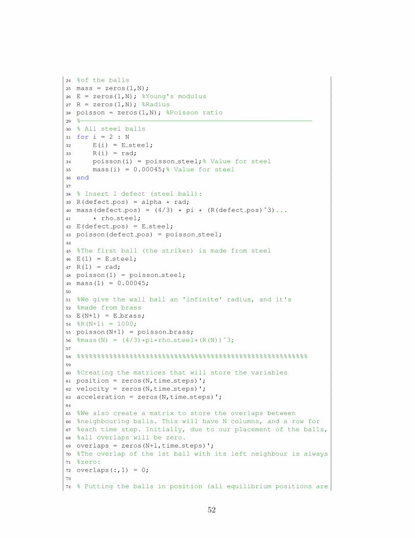
24 %of the balls25 mass = zeros(1,N);26 E = zeros(1,N); %Young's modulus27 R = zeros(1,N); %Radius28 poisson = zeros(1,N); %Poisson ratio29 %−−−−−−−−−−−−−−−−−−−−−−−−−−−−−−−−−−−−−−−−−−−−−−−−−−−−−−−−−30 % All steel balls31 for i = 2 : N32 E(i) = E steel;33 R(i) = rad;34 poisson(i) = poisson steel;% Value for steel35 mass(i) = 0.00045;% Value for steel36 end37
38 % Insert 1 defect (steel ball):39 R(defect pos) = alpha * rad;40 mass(defect pos) = (4/3) * pi * (R(defect pos)ˆ3)...41 * rho steel;42 E(defect pos) = E steel;43 poisson(defect pos) = poisson steel;44
45 %The first ball (the striker) is made from steel46 E(1) = E steel;47 R(1) = rad;48 poisson(1) = poisson steel;49 mass(1) = 0.00045;50
51 %We give the wall ball an 'infinite' radius, and it's52 %made from brass53 E(N+1) = E brass;54 %R(N+1) = 1000;55 poisson(N+1) = poisson brass;56 %mass(N) = (4/3)*pi*rho steel*(R(N))ˆ3;57
58 %%%%%%%%%%%%%%%%%%%%%%%%%%%%%%%%%%%%%%%%%%%%%%%%%%%%%%%%%59
60 %Creating the matrices that will store the variables61 position = zeros(N,time steps)';62 velocity = zeros(N,time steps)';63 acceleration = zeros(N,time steps)';64
65 %We also create a matrix to store the overlaps between66 %neighbouring balls. This will have N columns, and a row for67 %each time step. Initially, due to our placement of the balls,68 %all overlaps will be zero.69 overlaps = zeros(N+1,time steps)';70 %The overlap of the 1st ball with its left neighbour is always71 %zero:72 overlaps(:,1) = 0;73
74 % Putting the balls in position (all equilibrium positions are
52
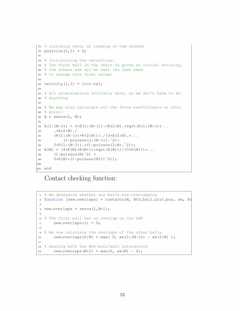
75 % initially zero, no loading in the system)76 position(1,1) = 0;77
78 % Initialising the velocities:79 % The first ball in the chain is given an initial velocity,80 % the others are all at rest (so just need81 % to change this first value)82
83 velocity(1,1) = init vel;84
85 % All accelerations initially zero, so we don't have to do86 % anything87
88 % We may also calculate all the force coefficients at this89 % point:90 A = zeros(1, N);91
92 A(1:(N−1)) = 4*E(1:(N−1)).*E(2:N).*sqrt(R(1:(N−1))...93 .*R(2:N)./94 (R(1:(N−1))+R(2:N)))./(3*E(2:N).*...95 (1−poisson(1:(N−1)).ˆ2)+96 3*E(1:(N−1)).*(1−poisson(2:N).ˆ2));97 A(N) = (4*E(N)*E(N+1)*sqrt(R(N)))/(3*E(N+1)*...98 (1−poisson(N)ˆ2) +99 3*E(N)*(1−poisson(N+1)ˆ2));
100
101 end
Contact checking function:
1 % We determine whether any balls are overlapping2 function [new overlaps] = contacts(N, Nth ball init pos, xx, R)3
4 new overlaps = zeros(1,N+1);5
6 % The first ball has no overlap on its LHS7 new overlaps(1) = 0;8
9 % We now calculate the overlaps of the other balls10 new overlaps(2:N) = max( 0, xx(1:(N−1)) − xx(2:N) );11
12 % Dealing with the Nth−ball/wall interaction13 new overlaps(N+1) = max(0, xx(N) − 0);
53
References
[1] R. Carretero-Gonzalez, D. Khatri, M.A. Porter, P.G. Kevrekidis, and
C. Daraio. Dissipative Solitary Waves in Granular Crystals. Physical
Review Letters, 102(2):024102, 2009.
[2] A. Chatterjee. Asymptotic Solution for Solitary Waves in a Chain of
Elastic Spheres. Physical Review E, 59(5):5912–5919, 1999.
[3] C. Coste, E. Falcon, and S. Fauve. Solitary waves in a chain of beads
under hertz contact. Physical Review E, 56(5):6104–6117, 1997.
[4] T. Cretegny, S. Aubry, and S. Flach. 1d Phonon Scattering by Discrete
Breathers. Physica D, 119(1-2):73 – 87, 1998.
[5] C. Daraio, V. F. Nesterenko, E. B. Herbold, and S. Jin. Strongly non-
linear waves in a chain of teflon beads. Physical Review E, 72(1):016603,
2005.
[6] U. Fano. Effects of configuration interaction on intensities and phase
shifts. Phys. Rev., 124(6):1866–1878, 1961.
[7] E. Fermi, J. Pasta, and S. Ulam. Studies of Nonlinear Problems. I. Los
Alamos Scientific Laboratory, Report LA-1940, 1955.
[8] S. Flach and A. Gorbach. Discrete Breathers in Fermi–Pasta–Ulam
lattices. Chaos, 15(1):015112, 2005.
[9] S. Flach and A. V. Gorbach. Discrete Breathers – Advances in theory
and applications. Physics Reports, 467(1-3):1 – 116, 2008.
[10] S. Flach, A. E. Miroshnichenko, and M. V. Fistul. Wave scattering by
Discrete Breathers. Chaos, 13(2):596–609, 2003.
[11] S. Flach and C. R. Willis. Discrete Breathers. arXiv:patt-sol/9704004v1,
1997.
[12] E. Hascoet and H.J. Herrmann. Shocks in Non-Loaded Bead Chains
with Impurities. The European Physical Journal B, 14(1):183 – 190,
2000.
54
[13] J. Hong and A. Xu. Nondestructive identification of impurities in gran-
ular medium. Applied Physics Letters, 81(25):4868–4870, 2002.
[14] S. Job, F. Melo, A. Sokolow, and S. Sen. Solitary wave trains in gran-
ular chains: Experiments, Theory and Simulations. Granular Matter,
10(1):13–20, 2007.
[15] S. Job, F. Santibanez, F. Tapia, and F. Melo. Wave Localization in
strongly nonlinear Hertzian chains with mass defect. arXiv:0901.3532v1,
2009.
[16] Charles Kittel. Introduction to Solid State Physics. Wiley, New York,
1996.
[17] L.D. Landau and E.M. Lifschitz. Theory of Elasticity. Pergamon, Ox-
ford, 1970.
[18] A.E.H. Love. A Treatise on the Mathematical Theory of Elasticity.
Dover, New York, Fourth edition, 2003.
[19] I. G. Main. Vibrations and Waves in Physics. CUP, Cambridge, Third
edition, 1993.
[20] A. E. Miroshnichenko, S. Flach, and Y. S. Kivshar. Fano resonances in
nanoscale structures. arXiv:0902.3014v4, 2009.
[21] U. Naether, D. E. Rivas, M. A. Larenas, M. I. Molina, and R. A. Vicen-
cio. Fano resonances in saturable waveguide arrays. arXiv:0906.1160v2,
2009.
[22] V. F. Nesterenko. Dynamics of Heterogeneous Materials. Springer-
Verlag, New York, 2001.
[23] V.F. Nesterenko. Propagation of Nonlinear Compression Pulses in
Granular Media. Journal of Applied Mechanics and Technical Physics,
24(5):733 – 743, 1983.
[24] L. Ponson, N. Bocchler, Y. Ming Lai, M.A. Porter, P.G. Kevrekidis, and
C. Daraio. Elastic Spin Chains. arXiv:0904.0426v1, 2009.
55
[25] M. A. Porter, C. Daraio, I. Szelengowicz, E. B. Herbold, and P.G.
Kevrekidis. Highly nonlinear solitary waves in heterogeneous periodic
granular media. Physica D, 238(6):666 – 676, 2009.
[26] M.A. Porter, N.J. Zabusky, B. Hu, and D.K. Campbell. Fermi, Pasta,
Ulam and the Birth of Experimental Mathematics. American Scientist,
97(6):214–221, 2009.
[27] S. Sen, J. Hong, J. Bang, E. Avalos, and R. Doney. Solitary Waves in
the Granular Chain. Physics Reports, 462(2):21 – 66, 2008.
[28] G. Theocharis, M. Kavousanakis, P.G. Kevrekidis, C. Daraio, M.A.
Porter, and I.G. Kevrekidis. Localized Breathing Modes in Granular
Crystals with Defects. arXiv:0906.4094v1, 2009.
[29] P. Tong, B. Li, and B. Hu. Wave transmission, phonon localization, and
heat conduction of a one-dimensional Frenkel-Kontorova chain. Physical
Review B, 59(13):8639–8645, 1999.
[30] G. B. Whitham. Linear and Nonlinear Waves. John Wiley & Sons,
1974.
56

![Nonlinear Counterpropagating Waves, Multisymplectic ...1].pdf · nonlinear counterpropagating waves, multisymplectic geometry, and the instability of standing waves∗ thomas j. bridges](https://img.pdfslide.us/doc/110x75/5b3b14a77f8b9a1a678e4c41/nonlinear-counterpropagating-waves-multisymplectic-1pdf-nonlinear-counterpropagating.jpg)