Nonlinear Soil Amplification: Its Corroboration in Taiwan

Bulletin of the Seismological Society of America, Vol. 85, No. 2, pp. 496-515, April 1995

Nonlinear Soil Amplification: Its Corroboration in Taiwan

by Igor A. Beresnev, Kuo-Liang Wen, and Yeong Tein Yeh

Abstract Nonlinear ground response at two strong-motion arrays in Taiwan is studied using the spectral ratio technique. At the SMART1 array, we calculate the frequency-dependent soil amplification functions as a ratio of the spectra at alluvium to rock sites, and study their dependence on the excitation level. Hor- izontal components of shear waves are considered. We compare (1) the average spectral ratios on weak and strong motions, (2) the ratios for the mainshocks and aftershocks, and (3) the ratios for the strong shear waves and their coda. At the SMART1 array, "weak motions" have a peak horizontal acceleration (PHA) less than 30 Gal. "Strong motions" are in the range of 100 to 267 Gal. Comparison of the average weak- and strong-motion spectral ratios shows a significant deamplification of strong motion between 2 and 9 Hz, exceeding the error margin estimated by the standard deviations. The maximum deamplification occurs at approximately 6.5 Hz where the average weak-motion amplification is 2.9 versus 0.40 in the strong motion. A similar pattern is exhibited by the ratios calculated for the mainshocks and the aftershocks, as well as for the shear waves and their coda. The spectral ratio calculated from a single realization of coda is identical to the average ratio obtained from many small earthquakes. At the SMART2, we analyze spectral ratios between the stations on Pleistocene terrace deposits and recent alluvium, which characterize the relative response at these two types of sediments. Weak motion is PHA less than 13 Gal, while strong motion extends from 100 to 295 Gal. Strong-motion spectral ratios between terrace and alluvial sites are consistently reduced in the frequency range from - 1 to 10 Hz, compared with the weak motion. This effect is insensitive to the variation in distance between stations from 7.9 to 11.4 km, as well as the azimuthal change of up to 80 ° in the station pair strike. We attribute the observed discrepancies between weak- and strong-motion amplifications to the differential nonlinear response occurring at terrace and alluvial sites. Our results document a significant nonlinear ground response at both arrays.

Introduction

Nonlinear effects in ground motion during large earthquakes have long been a controversial issue between seismologists and geotechnical engineers. Nonlin- ear effects have been routinely taken into account in earthquake engineering in the evaluation of seismic wave amplification by superficial deposits. However, seismologists rarely considered the possibility of these phenomena playing an important role (Aki and Richards, 1980, p. 9).

Explicit indications of the significance of nonlinear site response in seismological observations have appeared in the last years, owing to the progressive increase in the number of permanently operating strong- motion arrays and improvement in data quality. These

findings have increased seismological interest in the study of nonlinear seismic phenomena worldwide.

Linear and Nonlinear Amplification of Seismic Waves

That the amplitude of seismic waves approaching the earth's surface is magnified by superficial low-imped- ance layers is well understood. Works by Kanai et al.

(1956) and Gutenberg (1957) started a quantitative study of this phenomenon. The importance of soil amplification effects has been clearly demonstrated by the great recent Michoacan (Mexico) earthquake of 19 September 1985 (Celebi et a l . , 1987; Seed et a l . , 1988) and the

496

Nonlinear Soil Amplification: Its Corroboration in Taiwan 497

Loma Prieta (California) earthquake of 17 October 1989 (Borcherdt and Glassmoyer, 1992).

It has been known in geotechnical engineering that the soil response becomes nonlinear beyond a certain level of deformations. Stress-strain relationships in the range of shearing deformations produced by large earthquakes are nonlinear and hysteretic, as confirmed by numerous results of vibratory and cyclic loading tests performed on soil samples in many laboratories around the world. A typical stress-strain relationship in simple shear is shown in Figure 1. The experimentally recorded law is com- posed of an initial loading (skeleton)curve and of hysteresis loops developed upon subsequent unloading and reloading.

Two corollaries follow from the hysteretic material behavior. First, Figure 1 shows that the greater the maximum strain during the cycle, the lower the secant modulus Gscc. This means that the effective shear-wave velocity, that is defined by the shear modulus as V = V~G-~, where p is density, decreases as the strain increases. Second, hysteresis implies a loss of energy in each deformation cycle proportional to the area of the hysteretic loop. The increase in the maximum strain leads to the expansion of the loop that results in the increasing damping. In other words, not only the shear-wave velocity but also the damping in soil become dependent on wave amplitude if the nonlinearity is postulated.

How will the nonlinear deformation process mani- fest itself in seismological observation? Each surface layer overlying a rigid basement exhibits the resonances at the frequencies.

V f = (2n - 1) ~-~, (1)

where H is the layer thickness and n is a positive integer (Murphy et al., 1971, p. 114). Thus, resonance frequencies are proportional to the wave velocity and will be therefore shifted downward as the strain increases. Similarly, increased dissipation will reduce soil amplification in the strong motion compared to the weak motion (strong-motion deamplification effect).

A simple hyperbolic form of the initial loading curve is widely accepted in state-of-the-art soil engineering (broken line in Fig. 1):

Gm,~y r = f(~,) = , (2)

G.,,~ 1 ÷

"/'max

where ~- is the shear stress, y is the shear strain, Gm~x is the undisturbed modulus (tangent modulus at the origin in Fig. 1), and %,~ is the shear strength (the maximum stress that material can support in the initial state) (Har- din and Dmevich, 1972a, b; Yu et al., 1993). Yu et al.

(1993) used a public-domain computer code DESRA2 to outline the characteristic symptoms that distinguish linear and nonlinear responses in the soil model defined by equation (2). The differences in soil transfer functions are separated into three frequency bands. In the lowest range, the amplification is not affected by nonlinearity. In the central band, the nonlinear deamplification takes place. Finally, in the high frequencies, amplification is higher in nonlinear response than in the linear one.

The appearance of the specific frequency intervals where nonlinear and linear responses disagree can be predicted from simple qualitative reasonings. Indeed, in the low-frequency range, the wavelength is long enough and the waves do not really see the subsurface sediments. In the intermediate range, the extra attenuation of strong motions caused by hysteretic damping reduces their amplitudes relative to the weak motions. In the high- frequency band, this effect is counterbalanced by higher harmonics generation that increases strong-motion amplitudes. We give an idea of the plausible mechanism for higher harmonics generation in the Appendix. Ac- cording to these guidelines the observational seismological data can be inspected for the presence of nonlinear effects.

Geotechnical Constraints to Accept Nonlinear Soil Behavior

Nonlinear constitutive relation for soil originates from empirical data. Laboratory tests consistently show the reduction in shear moduli and increase in damping with increasing shear strain. Typical test data were published by Seed and Idriss (1969, 1970) and since then have

~0 r~

reloading branch _

Gmax

A Gsec

~ / ' / Shear Strain

/ \ unloading branch

Figure 1. Typical stress-strain relationship of soil in shear deformation (adapted from Moham- madioun and Pecker, 1984). Initial loading curve has a hyperbolic form (broken line). Subsequent unloading and reloading phases track a hysteretic path.

498 I.A. Beresnev, K.-L. Wen, and Y. T. Yeh

been extensively used in soil engineering. Modulus degradation and stress-dependent damping curves for different kinds of clays have been published by Iwasaki et

al. (1982) and Sun et al. (1988). Hardin and Drnevich (1972a, b) experimentally recorded hysteresis loops for a wide variety of soils. Typically, significant deviations from the linear elasticity occur at deformations larger than -10-2% (e.g., Erdik, 1987, Fig. 16).

Thus, nonlinear soil behavior above some acceleration level is postulated geotechnically. However, this is largely based on the results of the laboratory tests and the assumption that the in si tu materials behave likewise. Alternative literature similarly exists where the appli- cability of linear elastic models to strong ground-motion evaluation is substantiated (Tsai and Housner, 1970; Murphy et a l . , 1971; Joyner et a l . , 1981; Seale and Ar- chuleta, 1989). This can partly explain the origin of a continuous debate between seismologists and engineers about the significance of the nonlinear site effects (Finn, 1991, p. 205; Yu et a l . , 1993, p. 218). As Aki and Ir- ikura (1991, pp. 95-96) and Aki (1993, p. 108) state, seismologists are reluctant to accept the ground nonlinearity because the linear elastic models of seismic energy generation, propagation, and near-surface transforma- tion developed in seismology have worked reasonably well even at the strong-motion level.

What evidence of nonlinear soil behavior is needed to be considered as direct seismological evidence? One proof would demonstrate on real strong-motion records that the natural period and shear-wave velocity of sediments depend on the amplitude of excitation. Another proof would confirm that the empirical site amplification consistently diverges in weak and strong motions. Some of such evidence appeared recently, although the number of reliable observations remains scarce.

Existing Seismological Evidence of Nonlinear Site Response

Tokimatsu and Midorikawa (1981) were perhaps the first to demonstrate a shear modulus degradation effect at the strains of 10 -5 to 10 -3 from real strong-motion accelerograms. Their estimates were based on the observed fundamental periods, and the magnitude of the effect was within the range expected from the laboratory tests.

A question of nonlinear site amplification was ad- dressed by Jarpe et al. (1988) for accelerations up to 0.7 g using the aftershock data of the 1983 Coalinga (Cali- fornia) earthquake. Average alluvium to sandstone spectral ratios for 23 weak and seven strong events showed that the strong-motion amplification was significantly lower between --10 and 11 Hz. Nonlinear soil behavior was named as a most likely cause.

Singh et al. (1988) computed the spectral ratios between the soil station and the hill zone rocky station in Mexico City for the 1985 Michoacan earthquake and three

smaller events whose epicenters were about 300 km and more from the sites, that almost precluded the influence of source or path dissimilarities on the ratios. Singh et al. (1988, Fig. 2) pointed at the clear evidence of nonlinear clay behavior during the Michoacan earthquake. The corresponding spectral ratio was noticeably lower and peaks were shifted toward longer periods compared to the weak motions. The effect was distinct between 0.2 and 4 Hz.

The case of the Loma Prieta earthquake provides one of the most carefully established indications of the nonlinear elasticity of soil. Darragh and Shakal (1991) applied the spectral-ratio method to study the nonlinear response at Treasure Island and Gilroy number 2 soil sites with respect to the reference stations at Yerba Buena Is- land and Gilroy number 1, respectively. Treasure Island gave a much lower amplification in the Loma Prieta mainshock than in the subsequent aftershocks in the frequency range from 0.5 to 7 Hz, despite the relatively low PGA (peak ground acceleration) at the reference station of 0.07 g. The stiff alluvial site Gilroy number 2 displayed a less pronounced but still evident nonlinear effect.

Chin and Aki (1991) applied a stochastic modeling technique to simulate observed strong-motion accelerograms from the Loma Prieta earthquake. The observed and predicted accelerograms showed good agreement in their durations and spectral content; however, motions observed at soil sites at distances less than approximately 50 km from the epicenter had systematically smaller peak accelerations relative to the prediction. The authors attributed this disagreement to the deamplification that occurred in the Loma Prieta strong motions. The mean threshold acceleration beyond which Chin and Aki (1991) report the nonlinear behavior at soft sites is about 0.1 g, which did not contradict the geotechnical engineering expectations.

Chang et al. (1989) and Wen (1994) analyzed the spectral ratios of the surface to downhole accelerometers at the borehole drilled at the LSST (Lotung Large-Scale Seismic Test) sedimentary site in Taiwan (southwest quadrant of the SMART1 array). Using different tech- niques to backcalculate shear-wave velocities in the subsurface strata during strong shaking, Chang et al. (1989) observed their distinct dependence on acceleration amplitude. Shear moduli decreased to as low as 15 to 20% of the low-strain values as PGA at the surface reached the level of 0.21 g. The effect was clearly observed at all depths down to the bottom of the borehole at 47 m. Wen (1994) extended this study to the data set of 22 events recorded during the Lotung experiment. PGA's amounted to 0.26 g. The effect of shear-wave velocity reduction was studied in five acceleration windows, and the gradual decrease of velocities was clearly observed as amplitude increased from 0 to 50 Gal in the first window up to 200 to 260 Gal in the highest strain window.


Shear-wave velocities degraded to as little as 50% of their low-strain values.

In summary, geotechnical testing of soils and the limited seismological data obtained so far suggest that nonlinear soil behavior may become significant when surface accelerations exceed 0.1 to 0.2 g. Further direct seismological observations are needed to find out whether nonlinear site response is really pervasive. The aim of this study is to examine the validity of this hypothesis using the data from two Taiwan strong-motion arrays which have been recording local earthquakes progres- sively since 1980.

S MAR T1 and S M A R T 2 Strong Mot ion Arrays

The SMART1 seismic array was installed in the northeast corner of Taiwan (Fig. 2). It is a dense array of 39 force-balanced triaxial accelerometers configured in three concentric circles of radii 200, 1000, and 2000 m. There is one station at the center (C-00). All the stations are installed on the recent alluvial plain of the Lan- yang river with uniform site conditions. One station (E- 02) has been positioned outside the outer ring on the slate outcrop, and can be used as a reference rock station.

Abrahamson et al. (1987) give a detailed description of the SMART 1 array. The underlying geologic and velocity structures have been summarized by Wen and Yeh (1984). Figure 3 depicts a north-south cross section across the array. Elevations of the plain range from 5 to 20 m. Thickness of the top low-velocity soil layer is 9 to 15 m. The soils consist of sandy silt and silty sand with some gravel, and the stations are geotechnically classi- fied as "deep cohesionless soil sites." The second layer is alluvium. Basement rock is the Miocene Lushan formation with P-wave velocities of about 3300 to 4000 m / sec. Its outcropping to the south of the array has been occupied by the E-02 reference station.

A more detailed study of the subsurface structure has been carded out in the frame of the LSST project (Chang et al. , 1989; Wen, 1994). Borehole logs at the LSST site (Fig. 2, top) revealed that the shear-wave velocity gradually increased from - 1 1 0 m/sec at the surface to 200 to 220 m/sec at a depth of 18 m. Below, the shear-wave velocity increased to 250 to 280 m/sec at a depth of 60 m.

SMART1 ground motions were digitized as 12-bit words at 100 samples per second. The Nyquist frequency was 50 Hz, and the pre-event memory was set to 2.5 sec. All of the data underwent preprocessing that included baseline subtraction and high- and low-pass fil- tering with cut frequencies of 0.1 and 25 Hz, respectively.

The SMART1 array was in operation in the period of 1980 to 1990. It recorded 60 local earthquakes with local magnitudes ranging from 3.6 to 7.0 and hypocen-

tral distances from 2.2 to 151 km. The maximum acceleration recorded is 375 cm/sec 2.

The SMART2 accelerograph array (Beresnev et al. , 1994) is currently deployed at the eastern coast of Tai- wan around the city of Hualien starting from December 1990 (Fig. 2, bottom). The array consists of about 45 surface stations dispersed through the area of approximately 20 by 10 km. It does not have a regular geometric shape as SMART1; however, there is a dense subset of about 10 stations in its northern part. Among them, station 37 has one surface and three downhole instruments at depths of 50, 100, and 200 m.

All stations are equipped with Kinemetrics FBA-23 accelerometers with 16-bit SSR-1 three-channel recorders. The pre-event memory is set to 10 sec. Ground motions are digitized at 200 samples per second, so that the Nyquist frequency is 100 Hz. The cut frequency of the low-pass filter is increased to 50 Hz. These features ensure better data quality compared with the SMART1 accelerograms.

Detailed geologic structure beneath the SMART2 is less well known. A geologic map is shown in Figure 2. All the stations are located in the Longitudinal Valley bordering upon the late Paleozoic to Mesozoic Central Range to the west and the Miocene to Pliocene Coastal Range or the Pacific coast to the east. Elevations range from 6 m at station 1 to 91 m at station 36, showing a gradual lowering of the surface from the Central Range to the coast. Stations in the Valley are either on the Pleistocene terrace deposits or recent alluvium. The borehole drilled to 200 m in the vicinity of station 37 through the terrace deposits disclosed four layers. The upper one consists of sand with small gravel (0 to 7 m, Vs = 100 m/sec) , the second is gravel and mud with some sand (7 to 62 m, Vs = 400 m/sec) , the third is sand with clay and small gravel (62 to 150 m, Vs = 460 m/sec), and the fourth layer (below 150 m, Vs = 1060 m/sec) includes rock, pebble gravel, and sand. Bedrock was not encountered.

Over about 2 1/2 yr of operation, the SMART2 array has recorded about 220 events with local magnitudes ranging from 3.1 to 6.0 and hypocentral distances from 0.1 to 166 km. The maximum recorded acceleration is 317 Gal.

Me thod o f Site Response Analysis

In this study, we define the site response in terms of spectral ratios in which Fourier amplitude spectra of the acceleration at one station are divided by the spectra at the reference station. We compare the ratios calculated on weak and strong motions in order to determine whether any differences between them occur.

Each earthquake is characterized by a source spectrum and the wave path to the recording station. In the site response study, recordings of different events are not

500 I . A . Beresnev, K.-L. Wen, and Y. T. Yeh

S M A R T - 1

N

t LANYANG RIVER

I~ * LSST SITE Y • SMART| STATION

LOTUNG

TAIPEI

.OrUNG I "E0,

HUALIEN

EO2 I I

TAIWAN

24"04"

S M A R T - 2

24"00"

A T I O N

2 3 ° 5 0 , 121"30" 121"40'

Figure 2. Location and layout of SMART1 and SMART2 arrays in Taiwan. Q6 is the recent alluvium, Q4 are Pleistocene terrace deposits (gravel, sand, clay), Q] are Pleistocene sediments, MP is late Miocene to Pliocene rock, Mt is early Miocene agglomerate and sandstone, PM4.5 is late Paleozoic to Mesozoic schist, PM3 is late Paleozoic to Mesozoic limestone.


directly comparable unless source and path effects that may overshadow the site response are removed. The spectral-ratio method is a straightforward way to isolate the relative site effect.

If the stations are some distance apart, the ratio reduces the source and path effects that are common to the stations, leaving residuals caused by spatial variation in the source directivity and the difference in the propagation path, which are especially significant for local events. One way to quantify them is to calculate the average ratio and its standard deviation from an ensemble of local earthquakes. It would be reasonable to suppose then that the variations from a true site response due to the irreducible source and path effects are included in the value of standard deviation. If the comparison of the weak-motion and the strong-motion averages shows their discrepancy greater than the standard deviation, then this can be interpreted as a nonlinear effect.

We obtain the relative site response, corrected for the differential path effects caused by the attenuation and geometric spreading, using the expression (Jarpe et al . , 1988)

S1 gl rl

$ 2 g2 r 2

e ~ri-r2)y/vQ, (3)

where $1/$2 is the "true" site response, gi is the spectrum of the recorded motion, ri is the hypocentral distance, f is the frequency, V is the shear-wave velocity, and Q is the quality factor. In the subsequent calculation, we assume V = 3500 m/sec and a frequency-dependent Q = 225f k 1 that is characteristic to northeastern Taiwan (Wang, 1993). The choice of V and Q affects the spectral-ratio estimates. We varied V between 3.0 and 4.0 km/sec and Q between two observed extremes Q = 225f 11 and Q = 125f °'79 (Wang, 1993). The maximum differences in spectral ratios produced by these variations for a station spacing equal to 10 km are 4% at 1 Hz, 10% at 10 Hz, and 15% at 30 Hz. Strictly speaking, the used estimates of Q are valid for frequencies up to 10 Hz only. We extrapolate them to 30 Hz, which may not be precisely correct.

s 01

50 100

200

400

60C (m)

N SOIL ( 430-- 760m/s) . . . . . . . . . . . . . . . . . . . . . . . . . . . . . . . . . . . . . . . . . . . . . . 0

ALLUVIUM ( 1400-- 1700 rn/s ) 50

100 PLEISTOCENE FORMATION

~ ~ ( 1800-2000 m/s ) 200

LUSHAN ~ 400

0 - 600 (rn)

Figure 3. North-south profile of the structure beneath the SMART1 array.

The calculation of spectral ratios is carried out as follows: (1) an 8-sec window containing the shear wave is identified on the horizontal components; (2) the window is tapered on both sides using a 5% of window length half-bell cosine function; (3) the Fourier amplitude spectrum is calculated; (4) the spectrum is smoothed using a 3-point running Hanning average filter (Kanasewich, 1981, p. 456) having a width of approximately 0.1 and 0.2 Hz for the SMART1 and SMART2 records, respectively; and (5) the ratio of two smoothed spectra is then calculated and corrected using the formula (3). The number of smoothings was chosen empirically considering its visual effect on the spectral shape, and was equal to 40 for SMART1 and 80 for SMART2 spectra. In the figures below we plot the average horizontal spectral ratios, which are calculated by summing the squares of the ratios for the EW and NS components, dividing by 2, and taking the square root.

For all of the accelerograms where sufficiently long pre-event noise was recorded, we calculated the signal- to-noise ratio by dividing the smoothed amplitude spectra of the S-wave window and the pre-event noise. The reliable frequency band is defined as that band in which the signal-to-noise ratio is greater than 5. Examination of all the data gave a reliable frequency band of 1 to 10 Hz for the SMART1 and 1 to 30 Hz for the SMART2 records. Accordingly, the ratios are normally plotted in these bands, except for several cases where the reliable bands are wider.

At the SMART1 array, we take the ratios between the alluvial central station C-00 and the bedrock station E-02, spaced at 4.8 km. They represent an estimate of the amplification function of the sediments below the C- 00 site. One can see from Figure 2 that there are soil stations closer to E-02; for example, the distance between stations 0-07 and E-02 is 2.8 kin. The main reason for our choice was that C-00 was triggered 47 times while 0-07 was triggered only 32 times. The response at other SMART1 stations can be a topic of further anal- yses.

At the SMART2 array a bedrock station is not available. We examine the ratios at several station pairs, where one station is located on terrace deposits and one on alluvium. These ratios characterize the amplification at one type of soil relative to the other.

Soil Ampl i f ica t ion on W e a k and Strong Mot ion at S MA RT1 Array

Comparison of Average Amplification on Weak and Strong Motion

The events by the categories of weak and strong events are defined herein according to the peak surface acceleration. The SMARTI digital recorders have 2 g full scale with a 12-bit A / D converter. These parameters

502 I .A . Beresnev, K.-L. Wen, and Y. T. Yeh

Table 1 Selected SMART1 Events

Peak Acceler, C00/Peak Aceeler.

Event* and Date E-02 (Gal)

(m/d/yr) EW NS Mr. Depth A* (C-00)/A(E-02) (km) (km)

Weak Motion

25 (09/21/83) 27.8/19.6 28.0/19.8 6.8 32 (06/12/85) 19.5/6.1 17.9/13.5 6.0 34 (08/05/85) 17.6/15.4 20.9/12.1 5.8

Strong Motion

39 (01/16/86) 212.2/166.2 266.7/197.5 6.5 40 (05/20/86) 170.3/185.9 228.9/95.9 6.6 43 (07/30/86) 116.6/184.6 232.8/245.9 6.2 45 (11/14/86) 120.4/133.2 150.5/139.8 7.0

Aftershocks and Coda

40 coda* 35.7/12.0 32.8/13.1 41 (05/20/86) 35.8/32.5 50.6/49.1 6.2

43 coda* 25.6/9.2 31.0/9.6 44 (07/30/86) 31.7/17.2 45.9/20.8 4.9

18.0 100.5/96.9 5.3 48.5/48.2 1.3 34.4/30.1

10.2 24.4/27.0 15.8 69.7/65.1

1.6 6.0/3.7 13.9 77.3/72.7

21.8 74.2/69.6

2.3 5.4/4.3

*Event number corresponds to the original SMART1 classification. *Hypocentrat distance to the station in parenthesis. *Eight-seconds coda window starting at 8 sec after S-wave arrival.

25-30

39

A44

0 4 5

MAGNITUDE

7 0 ~ © 5 © 4

32 0

25 0

23-30 7 121-30 123-0

Figure 4. Epicenters of the SMARTI events selected for this analysis. The size of the circles scales with magnitude. Earthquakes that produced strong motions are distinguished by solid circles; weak motion earthquakes and aftershocks are shown by the open ones.

determine the minimum acceleration that can be recorded. Our visual inspection of the accelerograms evinced that motions with the PGA greater than - 1 0 Gal can be considered well recorded. Accordingly, we defined as weak motions those events that produced horizontal PGA's at both stations less or equal to 30 Gal, which should have satisfied the requirement of being well recorded. This upper value reflects a compromise between the necessity of acquiring as many events as possible, and the constraint that the event must remain weak. Three earthquakes that satisfied this criterion are shown in Table 1 (events 25, 32, and 34). Their minimum hypocentral distance to both stations is 30.1 kin.

According to the earlier seismological and geotechnical experience, departure from linearity can be roughly anticipated at accelerations beyond 100 Gal. Corre- spondingly, strong motions were selected if PGA's in EW and NS components at both stations exceeded this threshold. Keeping in mind that in stronger earthquakes the dimensions of the causative fault are larger, so that the f'mite-source effects in the spectral ratios may be more significant, we picked three strong events that were far- thest from the array. They are also tabulated in Table 1 (39, 40, and 45), the minimum hypocentral distance being 24.4 km. Overall peak horizontal acceleration is 267 Gal. Locations of all selected earthquakes relative to the array are shown in Figure 4. It is seen that they cover a variety of azimuths.

Figure 5 shows the average weak- and strong-motion spectral ratios calculated for these sets of events. Shaded bands represent + 1 standard deviation. To il-


lustrate how the smoothing procedure influences the shape of the function, we show the ratios corresponding to 5 and 40 smoothings at the top and the bottom of Figure 5, respectively, Smoothings were applied to individual ratios, not the averages. All subsequent SMART1 ratios are 40-fold smoothed.

Soil site amplifies the weak motion at all frequencies. Strong-motion ratios lie below the weak motion ones between - 2 and 9 Hz, the effect being larger than the error margin imposed by the standard deviation. The differences between weak- and strong-motion ratios are suggestive that nonlinear deamplification at the soil site took place. It is noteworthy that the strong-motion standard deviation above 2 Hz is generally lower than that

10 z

0

-4-O

o

u~

101

10 0

10-1

lO-e 1 10

10 e

I I I _

0 . , - - i

0

O3

101

10 0

10-1

10 -z 1 10

Frequency (Hz) Figure 5. Average weak-motion (thin line) and strong-motion (bold line) spectral ratios between soil and rock sites at SMART1 array. Three weak and three strong events are used to calculate the averages. Individual ratios have been computed as the geometric mean of the ratios for EW and NS components. Shaded areas represent - 1 S.D. about the average. Ratios shown at the top and the bottom correspond to 5 and 40 smoothings applied. Signal-to-noise proportion for all the frequencies is more than a factor of 5. Strong motions at the soil site are considerably deamplified between approximately 2 and 9 Hz compared with the weak motions, suggesting a nonlinear soil response.

in the weak motion, notwithstanding a wide variation in the azimuths of strong events. However, it is much higher below 2 Hz so that the ratios cannot be compared. Max- imum standard deviation in the weak motion curve at the bottom of Figure 4 is about 0.3 log units, which corresponds to a factor of 2.0.

Amplification drops below the uni ty value, turning into attenuation, between 4.5 and 7.5 Hz. Maximum deamplification occurs near 6.5 Hz where the average weak-motion amplification is 2.9 versus only 0.40 in the strong motion. Note that the arithmetic average of the peak EW and NS accelerations at the rock site in three strong events is 153 Gal. Nonlinear behavior of soil at this acceleration level can be indeed expected from existing experience.

Unfortunately, a collection of well-recorded weak events at the SMART1 array is not sufficient to provide a more representative statistics. The array was basically designed to document strong earthquakes. This limita- tion is overcome in the SMART2 case.

Comparison of Amplification in Mainshocks, Aftershocks, and Coda

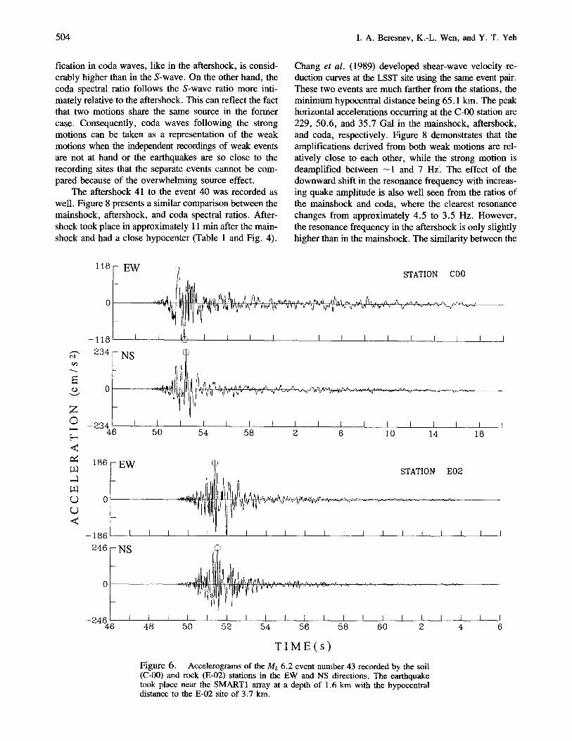
Event 43 (Table 1) took place in the proximity of the array and produced a peak horizontal acceleration of 246 Gal at the E-02 site. Recorded C-00 and E-02 accelerograms in the EW and NS directions are shown in Figure 6. Hypocentral distance to the E-02 station is just 3.7 km. This was a reason not to include this event in the plots in Figure 5. However, its aftershock (event 44, Table 1) occurred in about 7 min with almost coinciding hypocenter (Fig. 4), producing a PHA of 45.9 Gal. In the assumption that the source directivity pattern in these two events is similar, we compare their spectral ratios in Figure 7, where the thick line stands for the mainshock and the half-thick line for the aftershock. Strong motion is deamplified at almost the entire frequency range from 1 to 20 Hz, which is clear despite the possible over- shadowing of this effect by the differences in source radiation from two events. We attribute the discrepancy between strong- and weak-motion ratios to the manifes- tation of soil nonlinearity.

Also shown in Figure 7 (thin line) is the weak-motion amplification function calculated from the mainshock coda that immediately followed the S-wave window. Peak horizontal acceleration of 31.0 Gal in this part of accelerograms occurs at the C-00 site. Amplifi- cation functions calculated from coda have the advan- tage of representing the average of S-wave amplification for various directions of wave approach (Chin and Aki, 1991, p. 1861). Using a coda sample following a strong part of the accelerogram, we hypothesize that the linear- elastic soil response is restored after the termination of the strong shaking part where the motion is hysteretic. In fact, this conjecture is justified in Figure 7. Ampli-

504 I .A. Beresnev, K.-L. Wen, and Y. T. Yeh

fication in coda waves, like in the aftershock, is considerably higher than in the S-wave. On the other hand, the coda spectral ratio follows the S-wave ratio more inti- mately relative to the aftershock. This can reflect the fact that two motions share the same source in the former case. Consequently, coda waves following the strong motions can be taken as a representation of the weak motions when the independent recordings of weak events are not at hand or the earthquakes are so close to the recording sites that the separate events cannot be compared because of the overwhelming source effect.

The aftershock 41 to the event 40 was recorded as welt. Figure 8 presents a similar comparison between the mainshock, aftershock, and coda spectral ratios. After- shock took place in approximately 11 min after the mainshock and had a close hypocenter (Table 1 and Fig. 4).

Chang et al. (1989) developed shear-wave velocity reduction curves at the LSST site using the same event pair. These two events are much farther from the stations, the minimum hypocentral distance being 65.1 km. The peak horizontal accelerations occurring at the C-00 station are 229, 50.6, and 35.7 Gal in the mainshock, aftershock, and coda, respectively. Figure 8 demonstrates that the amplifications derived from both weak motions are relatively close to each other, while the strong motion is deamplified between ~ 1 and 7 Hz: The effect of the downward shift in the resonance frequency with increasing quake amplitude is also well seen from the ratios of the mainshock and coda, where the clearest resonance changes from approximately 4.5 to 3.5 Hz. However, the resonance frequency in the aftershock is only slightly higher than in the mainshock. The similarity between the

0

Z 0

< c~

. J U~

<

118

F EW

- 1 1 8 I

234 - NS

-231' 6

m

I

t t , I I ! I I I t I I I I I I

I I I I I 1 I I i I I I i I I 50 54 58 2 6 10 14 18

- 1 8 6 246

- 2 4 6 46

186 - EW

0

I

..... . , i 1

t

- N S

I I 48

E02

I , STATION

I I " ! I I I I I L I I i t I I

Jl

l ' ~ |

I I I I I I I I I I I i I I I I I I 50 5~ 54 56 58 60 2

I I

4 6

T I M E ( s )

Figure 6. Accelerograms of the ML 6.2 event number 43 recorded by the soil (C-00) and rock (E-02) stations in the EW and NS directions. The earthquake took place near the SMART1 array at a depth of 1.6 km with the hypocentral distance to the E-02 site of 3.7 kin.


weak-motion amplification functions suggests that the finite-source effects are not significant at these distances.

Soil Ampl i f ica t ion on W e a k and Strong Mot ion at S M A R T 2 Array

Due to the higher precision of the SMART2 instru- mentation, accelerograms with PGA equal to 2 to 3 Gal are considered well recorded, and consequently more weak-motion data are available. This permits a better statistical assessment of the variation in the weak-motion spectral ratios caused by factors different from the true site response.

In the following, we will compare the weak- and strong-motion spectral ratios between stations located on the Pleistocene terrace deposits and the recent alluvium in order to estimate the possible differences in their relative response due to nonlinear effects. Several pairs of such stations with different orientation in space will be chosen.

Weak- and Strong-Motion Amplification between Stations 3 and 36

Average Weak-Motion and Individual Strong-Motion Amplifications. Station 3 is located on Pleistocene terrace deposits at an elevation of 19 m. Station 36 is at the alluvial site that is close to the black schist Central Range outcrops at an elevation of 91 m (Fig. 2), albeit

10 2

0

~5

0 (1)

5Q

I0 i

10 o

I0-I

10-Z I I I I I I I I I I I I I I I I

1 10

Frequency (Hz) Figure 7. Spectral ratios between soil and rock stations at the SMART1 array calculated for the strong event 43 (thick line), its aftershock 44 (half- thick line), and S-wave coda of event 43 (thin line). Eight-seconds realization of coda, following the S-wave window, has been used. Signal-to-noise estimates allow extension of the usable frequency band to 20 Hz. Strong motion is deamplified at the soil site at almost all frequencies between 1 and 20 Hz in comparison with both weak motions, showing a nonlinear response.

the exact depth to the basement at this site is not known. Spacing between stations is 8.4 kin.

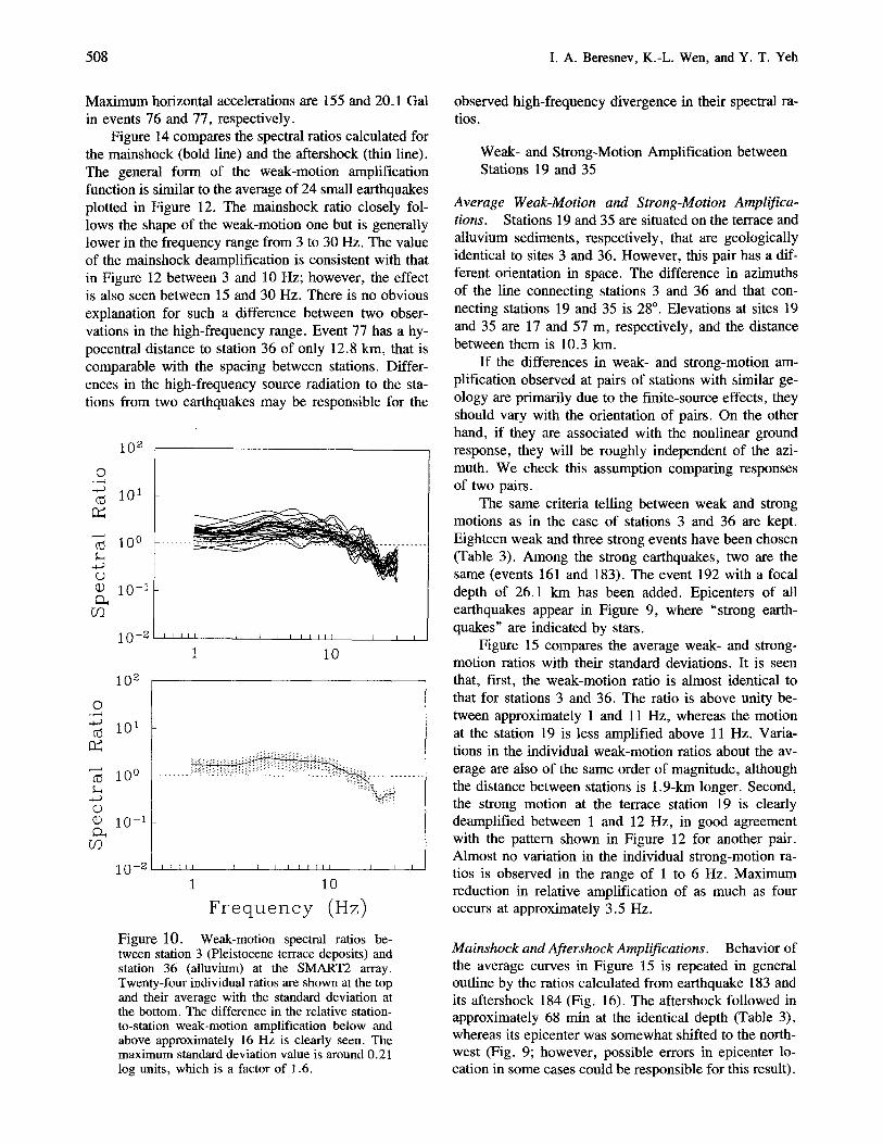
The individual event was attributed to the weak-motion class if the maximum horizontal acceleration at the stations in the pair did not exceed 13 Gal. This specific value has been chosen considering the necessity of gath- ering a sufficient number of weak-motion recordings. Twenty-four events fitting this requirement are listed in Table 2. Their locations are placed in Figure 9. Individ- ual ratios and their mean are plotted at the top of Figure 10. The mean and the standard deviation band are re- produced at the bottom of Figure 10. This plot shows that station 3 amplifies the weak motions below approximately 16 Hz and damps them between 16 and 30 Hz, relative to station 36. This observation may be due to the different surface geology at these sites. The maximum standard deviation of the weak-motion amplification is 0.21 log units, which corresponds to a factor of 1.6. This value is lower than in the SMART1 case, although the distance between stations has increased. The larger number of the events used in Figure 10 may have produced a more robust statistical estimate.

In selecting strong motions, we followed the same criterion as in the SMART1 case. The strong event was picked out if PGA's in EW and NS directions at both stations surpassed 100 Gal. Only two events met this requirement (events 161 and 183 in Table 2). Horizontal accelerograms of the earthquake 161 at stations 3 and 36 are exhibited in Figure 11. The choice of these events is especially favorable because both hypocenters are beneath the array at depths of 22.6 and 23.4 km, respec-

10 z

0

OQ

i0'

10 o

1 0 - I

1 0 - z I I 1 1 1 I I I t I I I I I I I

1 10

Frequency (Hz) Figure 8. Spectral ratios between soil and rock stations at the SMART1 array for the strong event 40 (thick line), its aftershock 41 (half-thick line), and S-wave coda of event 40 (thin line). Coda po- sition in the record is the same as in Figure 7. The longer hypocentral distance allows further reduction in source and path effects, which is reflected in the similarity of weak-motion ratios. Strong motion is deamplified between 1 and 7 Hz, showing a nonlinear response.


tively. The minimal hypocentral distance is 23.6 km, and the finite-source effects are believed to be insignificant.

Figure 12 compares the spectral ratios for two strong events with the average weak-motion ratio. Two observations are made. First, ratios produced by the strong motions are similar to each other. Second, strong motions at site 3 are largely deamplified compared with the weak motions in the frequency range from - 3 to 14 Hz. This effect is in excess of the uncertainty limits imposed by the standard deviation, and can be explained by the nonlinear behavior of soils underlying the two recording sites. Curiously, larger deamplification occurs at the terrace sediments than at younger alluvium which leads to a relative effect seen. The maximum average deampli-

fication is as much as 2.9 at 5.5 Hz (cf. a factor of 7.2 between the SMART1 soil and rock stations at 6.5 Hz). Unfortunately, geotechnical parameters of the sediments at these sites are unknown, so that the quantitative comparisons based on their physical properties cannot be made at this time.

Amplifications Derived from Coda Waves. Our aim is to infer again how the amplification function computed from the S-wave coda correlates with the average weak- motion amplification obtained from a representative number of small earthquakes. We calculate spectral ratios for the coda of earthquake 161 in the time windows starting at 4 and 8 sec after the S-wave arrival, where

Table 2 Selected SMART2 Events That Triggered Stations 36 and 3

Event* and Date (m/d/yr)

Peak Aeceler. 36/Peak Aeceler. 3 (Gal) Oepth

EW NS ML (kin)

56 (01/14/91) 59 (01/18/91) 60 (01/18/91) 62 (01/19/91) 63 (01/19/91) 64(01/19/91) 66 (01/20/91) 67 (01/21/91) 69 (01/21/91)

103(06/09/91) 110 (07/12/91) 113 (08/05/91) 117 (08/27/91) 118(08/27/91) 122 (09/21/91) 126 (10/08/91) 128 (10/14/91) 129 (10/15/91) 149 (01/11/92) 151 (01/29/92) 157 (03/09/92) 159 (03/11/92) 189 (07/23/92) 193 (08/17/92)

6.8/7.7 7.5/9.5 4.7/10.6 6.7/3.5 2.8/4.4 2.3/4.6 3.6 t3.8 4.4 ¢3.7 8.8 18.3 7.7/4.9

10.3/5.7 5.7/5.0 5.1/8.1 3.0/4.3 4.1/5.8 4.6/10.6 4.4/7.5 6.4/4.5 4.6/4.0

11.0/9.1 4.4/4.9 7.3/4.3

11.5/11.1 12.5/8.1

161 (03/21/92) 219.9/152.5 183 (06/25/92) 203.9/130.1

Weak Motion

3.4/11.4 9.4/11.0 4.6/5.4 5.5/4.2 4.0/5.1 3.8/5.4 4.6/5.2 4.6/3.4

12.2/7.0 7.3/6.9

12.3/8.2 8.5/5.9 5.5/8.2 4.9/6.7 4.8/8.7 4.4 4.0/9.8 4.5 5.2 ¢11.3 4.1 5.6/4.4 3.7 3.1/4.2 4.1 8.7/11.1 3.5 4.4 t4.0 4.3 5.9/4.7 3.3

12.9 tl l .7 4.7 12.5/11.0 4.3

Strong Motion

220.0/295.3 4.9 122.4/175.3 5.0

4.0 5.2 4.8 3.7 5.2 5.0 3.6 5.0 5.3 4.3 4.0 3.7 4.4 4.2

Other Mainshocks, Aftershocks, Coda

76 (02/25/91) i55.4/84.5 104.5/95.3 4.8 77 (02/25/91) 8.6/12.6 15.9/20.1 4.1

161 coda * 16,2/31.8 12.3/26.3 161 coda s 4.8/8.2 5.7/13.5

184 (06/25/92) 35.9126.3 19.2/31.8 3.8

0.9 0.9 3.3

12.6 5.6 2.3 8.8 2.6 2.9

10.7 10.1 13.5 7.4

13.3 12.5 16.3 8.8

10.1 34.3 16.1 22.3 12.6 21.2 22.6

22.6 23.4

16.8 11.7

23.3

*Event number corresponds to the original SMART2 classification. *Hypocentral distance to the station in parentheses. *Eight-seconds coda window starting at 4 sec after S-wave arrival. ~Eight-seconds coda window starting at 8 sec after S-wave arrival.

A*(36)/A(3) (kra)

16.7/11.9 38.0/45.3 38.9/46.8 14.6/20.0 29.8/32.0 28.1/29.7 11.1 ¢17.2 39.0/45.7 38.9/45.2 13.4 t19.4 13.1 q9.0 16.8/2t.0 28.3 t25.1 29.4 t22.5 30.1/23.1 30.2/25.5 19.0/12.8 11.8/17.7 41.2/37.2 16.2/18.5 26.1/23.1 13.8/13.6 24.9/26.8 25.2/26.9

24.6/24.0 26.1/23.6

17.4/21.1 12.8/18.0

26.9/24.7

Nonlinear Soil Amplification." Its Corroboration in Taiwan 507

peak horizontal accelerations are 31.8 and 13.5 Gal, respectively (Fig. 11 and Table 2). All the windows have a length of 8 sec. The S-wave spectral ratio and the average weak-motion ratio, both taken from Figure 12, are placed together with the coda ratios in Figure 13. A re- markable feature is that the single coda ratios fall within the shaded band around the average curve obtained from 24 weak earthquakes. Each of them diverges equally from the strong-motion ratio. This may be evidence that the amplification function obtained from the S-wave coda is

equivalent to the weak-motion amplification averaged over many small earthquakes.

Mainshock and Aftershock Amplifications. We seek independent confirmation of the presumable nonlinear effects disclosed in Figure 12 using available mainshock/ aftershock pairs. In the SMART2 data base, event 76 was followed by aftershock 77 that occurred within 27 rain with a contiguous hypocenter (Table 2, Fig. 9).

2 4 - 1 0

@

23-20 1 2 1 - 1 0

I I

60

59

67

69

I I I I I I

164

/ 192

I t " k , ,~ ,"4 =_

193 • • I I I (

189 1 • • • /

77 1 5 ) • ) 9 / 182

1 0 ~ 8 •

llO • ) 56

) 113 ]07

136

130

132

I

155

128

1 3 4

156 1 1 7

1¢9 118

114

126

I I I t /

1 2 2

0 10Kb I I

Figure 9. Epicenters of the SMART2 events selected for this analysis. Solid squares denote SMART2 stations. Events that produced strong motions are distinguished by stars; others are weak events and aftershocks.

1 2 2 - 0


Maximum horizontal accelerations are 155 and 20.1 Gal in events 76 and 77, respectively.

Figure 14 compares the spectral ratios calculated for the mainshock (bold line) and the aftershock (thin line). The general form of the weak-motion amplification function is similar to the average of 24 small earthquakes plotted in Figure 12. The mainshock ratio closely follows the shape of the weak-motion one but is generally lower in the frequency range from 3 to 30 Hz. The value of the mainshock deamplification is consistent with that in Figure 12 between 3 and 10 Hz; however, the effect is also seen between 15 and 30 Hz. There is no obvious explanation for such a difference between two observations in the high-frequency range. Event 77 has a hypocentral distance to station 36 of only 12.8 km, that is comparable with the spacing between stations. Differ- ences in the high-frequency source radiation to the stations from two earthquakes may be responsible for the

10 a

© . , - 4 - 4 - 0 <5 10~

, - - 4 10 °

..v..a

o ~o 10- I D~

lO-Z

i0 z

I I I I I

1 t I I I I I I I ~ I I I

10

0 - , - -4

oO I01

,-----4 I 0 °

0 10-~

1 0 - 2 I l l i l ~ t I I I I I l l I I

1 10

Frequency (Hz) Figure 10. Weak-motion spectral ratios between station 3 (Pleistocene terrace deposits) and station 36 (alluvium) at the SMART2 array. Twenty-four individual ratios are shown at the top and their average with the standard deviation at the bottom. The difference in the relative station- to-station weak-motion amplification below and above approximately 16 Hz is clearly seen. The maximum standard deviation value is around 0.21 log units, which is a factor of 1.6.

observed high-frequency divergence in their spectral ratios.

Weak- and Strong-Motion Amplification between Stations 19 and 35

Average Weak-Motion and Strong-Motion Amplifica- tions. Stations 19 and 35 are situated on the terrace and alluvium sediments, respectively, that are geologically identical to sites 3 and 36. However, this pair has a different orientation in space. The difference in azimuths of the line connecting stations 3 and 36 and that connecting stations 19 and 35 is 28 ° . Elevations at sites 19 and 35 are 17 and 57 m, respectively, and the distance between them is 10.3 km.

If the differences in weak- and strong-motion amplification observed at pairs of stations with similar geology are primarily due to the finite-source effects, they should vary with the orientation of pairs. On the other hand, if they are associated with the nonlinear ground response, they will be roughly independent of the azi- muth. We check this assumption comparing responses of two pairs.

The same criteria telling between weak and strong motions as in the case of stations 3 and 36 are kept. Eighteen weak and three strong events have been chosen (Table 3). Among the strong earthquakes, two are the same (events 161 and 183). The event 192 with a focal depth of 26.1 km has been added. Epicenters of all earthquakes appear in Figure 9, where "strong earthquakes" are indicated by stars.

Figure 15 compares the average weak- and strong- motion ratios with their standard deviations. It is seen that, first, the weak-motion ratio is almost identical to that for stations 3 and 36. The ratio is above unity between approximately 1 and 11 Hz, whereas the motion at the station 19 is less amplified above 11 Hz. Varia- tions in the individual weak-motion ratios about the average are also of the same order of magnitude, although the distance between stations is 1.9-km longer. Second, the strong motion at the terrace station 19 is clearly deamplified between 1 and 12 Hz, in good agreement with the pattern shown in Figure 12 for another pair. Almost no variation in the individual strong-motion ratios is observed in the range of 1 to 6 Hz. Maximum reduction in relative amplification of as much as four occurs at approximately 3.5 Hz.

Mainshock and Aftershock Amplifications. Behavior of the average curves in Figure 15 is repeated in general outline by the ratios calculated from earthquake 183 and its aftershock 184 (Fig. 16). The aftershock followed in approximately 68 min at the identical depth (Table 3), whereas its epicenter was somewhat shifted to the north- west (Fig. 9; however, possible errors in epicenter location in some cases could be responsible for this result).


Peak horizontal accelerations at the stations were 192 and 41.8 Gal in the mainshock and the aftershock, respectively. Decline in the strong-motion ratio in the frequency interval from 1 to 10 Hz is again clear from Fig- ure 16.

Comparison of Figures 12 through 14, on the one hand, and Figures 15 and 16, on the other hand, demonstrates that the differences in relative weak-motion and strong-motion amplification between terrace and alluvial deposits are roughly insensitive to the alignment of the station pair and variation of the distance between stations. This emphasizes that the differences in amplification are most probably caused by the effect of wave amplitude, not by the source directivity that might be significant in a few strong earthquakes considered in this analysis.

Weak- and Strong-Motion Amplification in Earthquakes 161 and 162

Finally, we verify the differences in weak- and strong- motion spectral ratios between terrace and alluvial sites

using event 161 and its aftershock 162. These earthquakes occurred at approximately the same depth of 22.6 and 24.8 km, respectively (Table 4). However, the aftershock epicenter seemingly moved approximately 13.1 km southeast of the mainshock (Fig. 9), so that the epicenters are located at opposite sides of the array (the same remark about the possible uncertainties in epicenter determination for weak earthquakes as above applies). This pair of earthquakes is of particular interest because earthquake 161 is one of the strongest events recorded by the SMART2 array. It caused an array-wide PHA of 311 Gal, while earthquake 162 produced just 5.9 Gal.

Among the stations triggered by both earthquakes, station 15 is on the recent alluvium and stations 20 and 33 are on Pleistocene deposits. The azimuthal difference in the alignment of pairs 20/15 and 33/15 is 33 °. Earth- quake 161 caused PHA's at sites 20, 33, and 15 of 79.8, 170, and 95.3 Gal, respectively. On the other hand, the corresponding accelerations in the aftershock were 3.8, 5.0, and 1.9 Gal (Table 4). We compare the relative

E O

Z

O

<

UJ

UJ

<

154 - EW

0 - -

- 1 5 4 I I

296 - NS

0 - -

- 2 9 6 I I 5 13

22O - EW

0

- 2 2 0 I 1

222 - N S

0

- 2 2 2 1 I 4 12

L,

r 3 , . ~

'~[',~r

Ill., l~,k.~i.,,..~L..

STATION 3

I ! I I I I I

~dJl. ....................

I I I I I I 21 29 37

STATION 36

. - I I ~ u . . . . . . .

|11111T1~ i . . . .

t I I I I I

~JL JLdl~ . . . . . . . . .

I I 2O

T I M E ( s )

I I I 28 36

Figure 11. Accelerograms of the ML 4.9 event 161 recorded by stations 3 and 36 in the EW and NS directions. The earthquake occurred beneath the SMART2 array at a depth of 22.6 km.

510 I .A . Beresnev, K.-L. Wen, and Y. T. Yeh

amplification at stations 20 and 33 with respect to station 15 at these contrasting acceleration levels.

Amplification at Station 20 Relative to Station 15. Two- station minimum hypocentral distances are 23.1 and 26.1

km for earthquakes 161 and 162, respectively. The distance between stations is 11.4 km. Mainshock and aftershock spectral ratios are shown in Figure 17. The shape of the ratios is similar in the whole frequency range, while the mainshock ratio is reduced between 1 and 7 Hz.

o

4.9 o ¢9

©

o q)

u~

10 2

I0 t

i0 o

i0-I

i0-2 , , , , ,

I

I I I I I I I I I I I

10

Frequency (Hz) Figure 12. Comparison of the average weak- motion spectral ratio between stations 3 and 36 (thin line) with the ratios calculated for two strong events (thick lines) at the SMART2 array. Strong- motion ratios deviate beyond the weak-motion standard deviation considerably in the frequency range from 3 to 14 Hz, showing a relative deamplification at the terrace deposits at site 3. This may be associated with the differential nonlinear soil behavior below the two stations.

10 z

101

I0 o

10-I

lO-Z i,,i,

1

I I I I I I I I I I

10

Frequency (Hz) Figure 13. Strong-motion amplification function for the event 161 (thick line), average weak- motion amplification function (thin line), both taken from Figure 12, together with the amplifications obtained from the S-wave coda of event 161 (other thin lines). Coda windows start at 4 and 8 sec after the S-wave arrival. It is seen that single coda amplifications are reliable estimates of the amplification function averaged over many small earthquakes.

I I

Amplification at Station 33 Relative to Station 15. Two- station minimum distances to the hypocenter are 22.9 and 26.1 km for the mainshock and the aftershock, respectively, which is almost identical to the preceding case. The separation distance is 7.9 km. Mainshock and aftershock ratios are shown in Figure 18. The curves differ from those in Figure 17. The weak-motion amplification is above unity for all the frequencies from 1 to 40 Hz. Since the denominator spectra in calculating correspond- ent ratios in Figures 17 and 18 are the same, the difference between them implies a change in the spectra at site 33 compared with site 20. It might be caused either by the variation in local geology, or the azimuthal variation in the source radiation. However, the mainshock curve is still reduced between 1 and 10 Hz in Figure 18. The amplitude dependence of the amplification seems to dominate the other changing conditions.

Thus, several independent examples show that the deamplification of the strong motion occurs at the site underlain by the terrace deposits, relative to the alluvial site. The relative amplification between - 1 and 10 Hz is insensitive to the rotation of the axis joining two stations and is apparently determined by the amplitude of the shaking developed at the surface. Since the curves in Figures 12 through 18 represent the response between two soil sites, the "deamplification" merely shows that terrace deposits exhibit a larger damping at high strains

10 z

0 .r..~

0 q)

CO

101

I0 o

10-I

1 0 - z , L L,,

1

. . . . . . . . . . . .

Figure 14. Spectral ratios for mainshock 76 and its aftershock 77. Deamplification of the mainshock at station 3 repeats the result of Figure 12. The usable frequency range stretches from 0.5 to 40 Hz in this example.

I I I , , I I I I I I I I I

10

Frequency (Hz)


than alluvial sediments. In this sense, the alluvial deposits behave as a more "linear" material in spite of their younger age, which seems paradoxical at first glance. However, the check using four station pairs showed that this effect was real.

Discussion

The goal of this study is to compare the amplification functions observed on weak and strong motions as

they emerge from the data of the SMART1 and SMART2 seismic arrays. In the analysis of the SMART1 records, we calculated amplifications of the soft alluvium site relative to the rock site. In the SMART2 case, where observations on rock sites have not been carded out, we compared amplifications on the terrace deposits with respect to the alluvial deposits. Significant divergences between the weak- and strong-motion amplification functions have been found in both cases.

Comparison of the average spectral ratios between

Table 3 Selected SMART2 Events That Triggered Stations 35 and 19

Peak Acceler. 35/Peak Acceler. 19 (Gal)

Event and Date Depth (m/d/yr) EW NS ML (kin)

Weak Motion

97 (04/22/91) 8.6/4.8 9.8/6.1 4.1 17.9 100 (05/05/91) 6.5/4.2 5.6/3.1 4.2 14.3 103 (06/09/91) 7.2/4.4 10.2/4.1 4.3 10.7 105 (06/19/91) 3.8/8.1 8.6/5.4 3.6 3.7 107 (06/28/91) 4.1/5.6 3.6/4.8 4.2 26.8 114 (08/08/91) 4.4/6.6 4.9/6.7 4.5 23.9 118 (08/27/91) 4.8/5.3 5.2/4.4 4.2 13.3 130 (10/18/91) 8.5/8.3 6.3/6.7 4.8 9.9 132 (11/03/91) 4.8/4.2 4.4/3.5 4.7 34.6 134 (11/04/91) 8.9/5.1 6.4/5.5 4.5 7.6 136 (11/07/91) 4.3/7.7 4.1/4.6 3.1 4.8 138 (11/24/91) 7.7/8.0 5.8/4.7 4.0 12.0 153 (02/21/92) 4.5/3.4 2.7/3.0 4.6 40.7 155 (03/03/92) 5.2/7.8 4.1/6.0 4.7 22.7 156 (03/04/92) 7.1/4.6 6.6/4.1 4.9 24.5 157 (03/09/92) 8.8/8.3 5.3/12.8 4.3 22.3 160 (03/15/92) 2.4/3.3 3.4/3.8 5.5 47.2 164 (04/02/92) 3.7/4.7 3.4/3.9 4.4 22.1

Strong Motion

161 (03/21/92) 170.1/132.1 249.2/217.7 4.9 22.6 183 (06/25/92) 147.6/106.3 191.9/106.1 5.0 23.4 192 (08/14/92) 159.4/132.1 149.4/111.3 5.2 26.1

Aftershock

184 (06/25/92) 41.8/16.5 21.4/14. l 3.8 23.3

*Hypocentral distance to the station in parentheses.

A*(35)/A(19) (km)

18.5/21.4 32.8/39.4 15.1/23.6 7.1 ¢5.8

31.8 ¢34.1 32.4 ¢30.6 27.9 123.0 23.4126.9 68.3/74.5 26.0/28.6 18.5/28.6 32.1/24.3 84.7/91.4 78.8/84.7 35.7/38.2 24.8/22.5

172.1/168.3 31.4/25.1

23.7/23.3 25.2/24.2 28.2/26.2

25.6/23.3

Table 4 Selected SMART2 Station Pairs Triggered by Events 161 and 162

Peak Accelerations in Pair

(Gal) Depth

Event EW NS M L (Ion)

Stations 15/20

161 47.7/79.1 95.3/79.8 4.9 22.6 162 1.7/2.9 1.9/3.8 3.7 24.8

Stations 15/33

t61 47.7/55.4 95.3/170.1 4.9 22.6 162 1.7/3.7 1.9/5.0 3.7 24.8

Hypocentral Distances for the Pair (km)

25.3/23.1 26.1/26.7

25.3/22.9 26.1/27.3

512 I .A . Beresnev, K.,L. Wen, and Y. T. Yeh

10 ~

0

o

[/3

101

10 o

10-1

lO-Z I I I I I I I I I I I I I I I I

i i0

Frequency (Hz) Figure 15. Average weak- (thin line) and strong-motion (bold line) spectral ratios between stations 19 and 35 at the SMART2 array. Stations 19 and 35 have geologies similar to those of stations 3 and 36, respectively, but their spatial alignment is different. The strong-motion ratio is reduced between approximately 1 and 12 Hz. Its deviation from the weak motion is consistent with Figure 12 in both the frequency range and magnitude. Agreement between two observations shows that nonlinear ground response, not the azimuthal variation in the source directivity, is the likely cause for the strong-motion ratio reduction.

10 ~

0 . , , - 4

0

101

10 o

10-1

1 0 - z I I I I I - I I I I I I I I I I I

1 10

Frequency (Hz) Figure 16. Spectral ratios for mainshock 183 and its aftershock 184. The strong-motion ratio is reduced in the frequency range from 1 to 10 Hz in agreement with Figure 15, while there are no obvious differences above 10 Hz. The reliable high- frequency range is up to 50 Hz.

alluvial and rock sites in the SMART1 array, calculated for three weak and three strong events, clearly demonstrates the reduction in the strong-motion ratio between approximately 2 and 9 Hz that exceeds the error margin dictated by the standard deviation. Strong accelerograms selected have a minimum horizontal acceleration of more

10 z

o

C) q)

cf~

101

10 o

10-1

1 0 - z I I I I I I I I I I I I I I I I

1 10

Frequency (Hz) Figure 17. Spectral ratios between sites 20 (terrace deposits) and 15 (alluvium) in mainshock 161 (bold line) and aftershock 162 (thin line). The spectral ratio for the mainshock is reduced, showing a deamplification at the terrace site.

10 z

0 ° , - -~

(6

o

D~ rf~

101

10 0

i 0 - I

1 0 - z I I I I I I I I I I I I l l I I

1 10

Frequency (Hz) Figure 18. Spectral ratios between sites 33 (terrace deposits) and 15 (alluvium) in mainshock 161 (bold line) and aftershock 162 (thin line). Dif- ferences in the weak-motion and strong-motion responses in the frequency range of approximately 1 to 10 Hz agree well with those observed at three other pairs of the SMART2 stations having different spatial orientation, showing that they are caused by the nonlinear deamplification produced by large-amplitude shaking at terrace deposits.

than 100 Gal. Maximum deamplification effect is observed near 6.5 Hz, where the difference between the weak- and strong-motion amplifications amounts to a factor of 7.2. The average strong-motion ratio falls off below the unity value in the frequency range from 4.5 to 7.5 Hz, which agrees with the recent data on soil response during the 1985 Michoacan and 1989 Loma Prieta earthquakes. It is important that the individual ratios calculated for the mainshocks, and their aftershocks and


shear-wave coda, exhibit the same general differences as do the average weak- and strong-motion ratios.

The SMART2 array provides an opportunity of a more thorough statistical analysis because of a larger number of small earthquakes recorded. It turns out that the variations in weak-motion spectral ratios, calculated for a variety of azimuths and hypocentral distances of earthquakes, have a rather modest value. For instance, the standard deviation of the weak-motion spectral ratio between stations 3 and 36, computed for 24 individual events, has a maximum value of about 0.21 log units (a factor of 1.6). We assume that the inherent source and path effects, which are irreducible by dividing the spectra, determine the value of this uncertainty and are im- plicitly included in it.

Significant differences in weak- and strong-motion spectral ratios appear on four geologically uniform station pairs, where the ratio of the spectrum at the terrace deposit site to the alluvium site is always taken. Re- gardless of the spatial orientation of a given pair the strong- motion ratio is always reduced in the frequency range be tween-1 and 10 Hz. This prevalent effect is insensitive to the variation in the distance between stations from 7.9 to 11.4 km, as well as to the rotation in the pair strike of up to 79 ° . Comparisons of the average weak- and strong-motion ratios, as well as the ratios for the mainshocks, aftershocks,~ and coda, support this conclu- sion. We attribute the observed strong-motion deamplification at the SMART2 pairs to the differential nonlinear response occurring at the terrace and alluvial sediments, that manifests itself as the apparent relative deamplification at the terrace site.

In most cases, we clearly see the existence of at least two distinctive frequency intervals contrasting the linear and nonlinear responses, similar to those discussed by Yu et al. (1993, p. 240). As a rule, ratios are not affected by nonlinearity at frequencies below 1 to 2 Hz [cf. 0.8 to 2.5 Hz for a corresponding cross-over frequency in Yu et a l . ' s (1993) theoretical modeling]. Physical explanation of this fact is clear: at the frequencies well below the natural one the wavelength of the incident waves is so long that the subsurface layers become "invisible" to them. In the central frequency band, very roughly between 1 and 10 Hz, the departure between the weak- and strong-motion ratios turns up. Fi- nally, spectral ratios converge again at frequencies higher than approximately 10 to 20 Hz [7 to 25 Hz in Yu et

al. 's (1993) report]. We have not observed the increased strong-motion ratios compared with those in weak motion in the high-frequency range, as Yu et al. (1993) predict, which could be accounted for by the nonlinear generation of higher harmonics (see Appendix). Unfa- vorable signal-to-noise ratios in this frequency range may have not permitted the observation of this effect. An- other explanation is that the competing effect of atten-

uation could make up for the increase in strong-motion ratios in the high frequencies.

We have shown by a direct comparison that the weak- motion amplification function derived from the S-wave coda in the strong-motion accelerogram is almost identical to the average amplification calculated from a large number of independent small earthquakes. Two corollaries are drawn from this fact. First, coda amplification can be regarded as an amplification of weak shear waves averaged over various angles of wave approach. Second, this proves that the motion ensuing a strong shear wave can be considered unaffected by the foregoing largely hysteretic oscillations, so that the linear soil response is recovered in coda.

Acknowledgments

We wish to thank Dr. H.-C. Chiu and the technical staff of the Institute of Earth Sciences of Academia Sinica who are in charge of the operation of the SMART2 array. Corrected accelerograms were prepared by W. G. Huang and the data processing group. We are also indebted to Mr. Huang for the assistance in preparing maps. Special thanks go to two reviewers for their constructive comments. This work was supported by the National Science Council, R.O.C. under Grant Numbers NSC 82-0202-M-001-132 and NSC 83-0202-M-001-0tM.

References

Abrahamson, N. A., B. A. Bolt, R. B. Darragh, J. Penzien, and Y. B. Tsai (1987). The SMARTI accelerograph array (1980-1987), a review, Earthquake Spectra 3, 263-287.

Aki, K. (1993). Local site effects on weak and strong ground motions, Tectonophysics 218, 93-111.

Aki, K. and K. Irikura (1991). Characterization and mapping of earthquake shaking for seismic zonation, in Proc. of the 4th Int. Conf. on Seismic Zonation, Stanford, California, Vol. 1, 61-110.

Aki, K. and P. Richards (1980). Quantitative Seismology. Theory and Methods, W. H. Freeman and Company, San Francisco.

Beresnev, I. A., K.-L. Wen, and Y. T. Yeh (1994). Source, path, and site effects on dominant frequency and spatial variation of strong ground motion recorded by SMART1 and SMART2 arrays in Taiwan, Earthquake Eng. Struct. Dyn. 23, 583-597.

Borcherdt, R. D. and G. Glassmoyer (1992). On the characteristics of local geology and their influence on ground motions generated by the Loma Prieta earthquake in the San Francisco Bay region, California, Bull. Seism. Soc. Am. 82, 603-641.

Celebi, M., J. Prince, C. Dietel, M. Onate, and G. Chavez (1987). The culprit in Mexico City--amplification of motions, Earth- quake Spectra 3, 315-328.

Chang, C.-Y., M. S. Power, Y. K. Tang, and C. M. Mok (1989). Evidence of nonlinear soil response during a moderate earthquake, in Proc. of the 12th Int. Conf. on Soil Mechanics and Foundation Engineering, Rio de Janeiro, Brazil, Vol. 3, 1-4.

Chin, B.-H. and K. Aki (1991). Simultaneous study of the source, path, and site effects on strong ground motion during the 1989 Loma Prieta earthquake: a preliminary result on pervasive nonlinear site effects, Bull. Seism. Soc. Am. 81, 1859-1884.

Darragh, R. B. and A. F. Shakal (1991). The site response of two rock and soil station pairs to strong and weak ground motion, Bull. Seism. Soc. Am. 81, 1885-1899.

Erdik, M. (1987). Site response analysis, in Strong Ground Motion Seismology, M. O. Erdik and M. N. Toksrz (Editors), D. Reidel Publishing Company, Dordrecht, Netherlands, 479-534.

514 I . A . Beresnev, K.-L. Wen, and Y. T. Yeh

Finn, W. D. L. (1991). Geotechnical engineering aspects of micro- zonation, in Proc. of the 4th Int. Conf. on Seismic Zonation, Stanford, California, Vol. 1, 199-259.

Gutenberg, B. (1957). Effects of ground on earthquake motion, Bull. Seism. Soc. Am. 47, 221-250.

Hardin, B. O. and V. P. Drnevich (1972a). Shear modulus and damping in soil: measurement and parameter effects, J. Soil Mech. Found. Div. ASCE 98, 603-624.

Hardin, B. O. and V. P. Drnevich (1972b). Shear modulus and damping in soil: design equations and curves, J. Soil Mech. Found. Div. ASCE 98, 667-692.

Iwasaki, T., K. Kawashima, and F. Tatsuoka (1982). Nonlinear seismic response analysis of soft soil deposits, in Proc. of the 7th European Conf. on Earthquake Engineering, Athens, Greece.

Jarpe, S. P., C. H. Cramer, B. E. Tucker, and A. F. Shakal (1988). A comparison of observations of ground response to weak and strong ground motion at Coalinga, California, Bull. Seism. Soc. Am. 78, 421-435.

Jones, G. L. and D. R. Kobett (1963). Interaction of elastic waves in an isotropic solid, J. Acoust. Soc. Am. 35, 5-10.

Joyner, W. B., R. E. Warrick, and T. E. Fumal (1981). The effect of quaternary alluvium on strong ground motion in the Coyote Lake, California, earthquake of 1979, Bull. Seism. Soc. Am. 71, 1333-1349.

Kanai, K., R. Takahasi, and H. Kawasumi (1956). Seismic characteristics of ground, in Proc. of the Worm Conf. on Earthquake Engineering, Berkeley, California, 31 - 1-31-16.

Kanasewich, E. R. (1981). Time Sequence Analysis in Geophysics, The University of Alberta Press, Winnipeg, Canada.

Mohammadioun, B. and A. Pecker (1984). Low-frequency transfer of seismic energy by superficial soil deposits and soft rocks, Earthquake Eng. Struct. Dyn. 12, 537-564.

Murphy, J. R., A, H. Davis, and N. L. Weaver (1971). Amplification of seismic body waves by low-velocity surface layers, Bull. Seism. Soc. Am. 61, 109-145.

Seale, S. H. and R. J. Archuleta (1989). Site amplification and attenuation of strong ground motion, Bull. Seism. Soc. Am. 79, 1673-1696.

Seed, H. B. and I. M. Idriss (1969). The influence of soil conditions on ground motions during earthquakes, J. Soil Mech. Found. Div. ASCE 94, 93-137.

Seed, H. B. and I. M. Idriss (1970). Soil moduli and damping factors for dynamic response analysis, Report No. EERC 70-10, Earth- quake Engineering Research Center, University of California, Berkeley.

Seed, H. B., M. P. Romo, J. I. Sun, A. Jaime, and J. Lysmer (1988). The Mexico Earthquake of September 19, 1985--relationships between soil conditions and earthquake ground motions, Earth- quake Spectra 4, 687-729.

Singh, S. K., J. Lermo, T. Dominguez, M. Ordaz, J. M. Espinosa, E. Mena, and R. Quaas (1988). The Mexico earthquake of Sep- tember 19, 1985--a study of amplification of seismic waves in the Valley of Mexico with respect to a hill zone site, Earthquake Spectra 4, 653-673.

Sun, J. I., R. Golesorkhi, and H. B. Seed (1988). Dynamic moduli and damping ratios for cohesive soils, Report No. UCB/EERC- 88/15, Department of Civil Engineering, University of Califor- nia, Berkeley.

Tokimatsu, K. and S. Midorikawa (1981). Nonlinear soil properties estimated from strong motion accelerograms, in Proc. of the Int. Conf. on Recent Advances in Geotechnical Earthquake Engi- neering and Soil Dynamics, St. Louis, Missouri, Vol. 1, 117- 122.

Tsai, N. C. and G. W. Housner (1970). Calculation of surface motions of a layered half-space, Bull. Seism. Soc. Am. 60, 1625- 1651.

Wang, J.-H. (1993). Q values of Taiwan: a review, J. Geol. Soc. China (Taiwan) 36, 15-24.

Wen, K.-L. (1994). Nonlinear soil response in ground motions, Earthquake Eng. Struct. Dyn. 23, 599-608.

Wen, K.-L. and Y. T. Yeh (1984). Seismic velocity structure beneath the SMARTI array, Bull. Inst. Earth Sci. Academia Sinica (Tai- wan) 4, 51-72.

Yu, G., J. G. Anderson, and R. Siddharthan (1993). On the characteristics of nonlinear soil response, Bull. Seism. Soc. Am. 83, 218-244.

Appendix

A tentative mechanism that leads to the increase in high-frequency content in the strong-motion spectra relative to the weak motions is proposed in this Appendix.

Seismic response of the soil in the 1D case is a solution of the equation of motion

02u Or - ( A 1 )

Po Ot 2 OZ'

where u is the horizontal displacement in shear wave

which propagates along the vertical axis z, P0 is undis-

turbed material density, and ~- is the shear stress. From the constitutive relation (2), assuming small deforma-

tions and using the b inomial expansion,

o- o_ ( ° - ) ~ - - - G~a~3' 1 3/ , (A2) ~'max

1 + - - 3 ' ~'m~

where the series is truncated, leaving only terms to the

second order in strain.

Defining strain as 3' = Ou/Oz, we obtain from equation (A2)

Or 02u (Gmax) z Ou 02u - - = G ~ a ~ - - 2 - ( A 3 ) OZ 0 7.2 Tmax OZ OZ 2"

This gives the fol lowing equation of motion from equation (A1):

02U 02U GZ,~Ou 02u Po ~-~ - G . ~ - - = - 2 - - ( A 4 )

0Z 2 Tma x 0Z 0Z 2"

Equation (A4) without the right-hand side represents a l inear wave equation. To have a notion of what kind

of solution a full nonl inear equation has, we seek its ap- proximate form using a perturbation method. Let u0 be a solution of the homogeneous equation (A4). Fol lowing a general idea of the perturbation method (e.g., Jones and Kobett , 1963, p. 6), we look for a small correction u ' to the l inear solution uo, introduced by the presence of the nonl inear term in equation (A4), as a solution of the inhomogeneous linear equation where uo is substi-


tuted into the right-hand side. This leads to the disturbed equation

OZu ' OZu ' G~o~ dUo 02//0 - - - G , . o ~ - 2 - - ( A 5 )

Po Ot s OZ 2 Tma x OZ OZ 2"

Let us take Uo as the sum of two harmonic waves with angular frequencies 0)1 and o92, wavenumbers kl and k2, and amplitude A:

Uo = A[sin (0)1t - k lz) + sin (o~t - k2z)]. (A6)

Substitution of equation (A6) into the right-hand side of equation (A5) gives

02U ' 02//' A2(72 P0 ~ - Gmax - - - v,,~x {k~ sin 2(0)1t - klz)

0Z 2 'i'ma x

+ k 3 sin 2(0)2t - ksz) + klkz(kl + kz)

sin[(0)~ + 0)2)t - (k~ + ks)z] + k~ks(k~ - ks)

sin[(0)1 - 0)0t - (k~ - k2)z]}. (A7)

The solution u' to the linear wave equation (A7) with the "driving force" terms determined by its right-hand

side will be the waves with the frequencies 20)1, 20)2, 0)1 - o92, and 0)1 "~- 0)2. In the real broadband earthquake signal, each individual frequency in the spectrum will generate its double frequency and the sum and difference with every other frequency. As a result, the source spectrum will expand to both low- and high-frequency ranges.

Low-frequency contribution from the nonlinearity will be of no importance because the surface layers have a finite thickness and the long-period waves will not ob- serve them. On the other hand, nonlinear generation of higher and sum harmonics will increase the values of the spectra at high frequencies in strong motions compared with the weak motions. This high-frequency amplification will appear most clearly above the comer frequency of the source spectra. Whether or not this effect will be realistically seen in the spectral ratios depends on the balance of the high-frequency generation and the competing effect of attenuation. Note that hysteretic char- acter of deformation is not required to produce the high- frequency generation effect.

Institute of Earth Sciences Academia Sinica P.O. Box 1-55 Nankang, Taipei 11529 Taiwan

Manuscript received 25 October 1993.

Documents

Nonlinear Soil Amplification: Its Corroboration in Taiwan