Embed Size (px)
Citation preview
Nonlinear Quantum Optics in Artificially StructuredMedia
by
Lukas Gordon Helt
A thesis submitted in conformity with the requirementsfor the degree of Doctor of Philosophy
Graduate Department of PhysicsUniversity of Toronto
c⃝ Copyright 2013 by Lukas Gordon Helt
Abstract
Nonlinear Quantum Optics in Artificially Structured Media
Lukas Gordon Helt
Doctor of Philosophy
Graduate Department of Physics
University of Toronto
2013
This thesis presents an analysis of photon pairs generated via either spontaneous para-
metric downconversion or spontaneous four-wave mixing in channel waveguides as well as
in microring resonators side-coupled to channel waveguides. The state of photons exiting
a particular device is calculated within a general Hamiltonian formalism that simplifies
the link between quantum nonlinear optics experiments and classical nonlinear optics ex-
periments. This state contains information regarding photon pair production efficiency
as well as modal and spectral correlations between the two photons, characterized by a
two-dimensional spectral distribution function called the biphoton wave function.
In the limit of a low probability of pair production, photon pair production efficien-
cies are cast into forms resembling corresponding well-known classical nonlinear optical
frequency conversion efficiencies, making it easy to see what plays the role of a classical
“seed” field in an un-seeded (quantum) process. This also allows photon pair production
efficiencies to be calculated based on the results of classical nonlinear optical experiments.
It is further calculated that, unless generated photons are collected over a very narrow fre-
quency range, their generation efficiency does not scale the same way with device length
in a channel waveguide, or resonance quality factor in a microring resonator, as might
be expected from the corresponding classical frequency conversion efficiency. Although
calculations do not include self- or cross-phase modulation, nor two-photon absorption
or free-carrier absorption, it is calculated that their neglect is justified in the low pair
production probability limit. Linear (scattering) loss is also neglected, though partially
addressed in the final chapter of this thesis.
ii
Biphoton wave functions are calculated explicitly, such that their shape and orien-
tation, including approximate analytic expressions for their widths, can easily be deter-
mined. This further allows estimation of the suitability of their associated photon pairs
for various quantum information processing applications. As an alternative to dispersion
engineering a channel waveguide photon pair source, it is calculated that microring res-
onators can very naturally produce nearly spectrally uncorrelated photon pairs, which
behave very much like idealized single-mode photons and are thus useful for applications
involving the interference of photons from multiple sources.
iii
Acknowledgements
Thanks must go to my principal supervisor, John Sipe, for his inspiration, guidance,
and support. I will leave the University of Toronto in 2013 with a PhD every bit as
excited about and interested in quantum mechanics as I became during his undergraduate
lectures back in 2004. I also would like to thank my co-supervisors Amr Helmy and Daniel
James for helping me stay on track as well as numerous useful comments and suggestions.
This thesis is better for them.
Thanks also goes to the excellent postdoctoral fellows of John’s Marco Liscidini and
Sergei Zhukovsky that I worked with at the University of Toronto. You are both hugely
responsible for shaping my methodology and outlook towards physics research, as well
as many of the successes of my PhD. I look forward to continuing to work with both of
you.
Thanks to Mike Steel, for inviting me to come visit Australia and hosting me at
Macquarie University for 9 weeks in 2012. It was an incredibly rewarding experience that
has led, and will hopefully continue to lead, to many interesting collaborations. Thanks
also goes to his PhD student Thomas Meany, who kindly invited me out to experience the
city, and all of the MQ Photonics and CUDOS teams, in particular Alex Clark, Chunle
Xiong, and Chad Husko, for their hospitality and many interesting discussions.
Thanks to my (largely experimental) collaborators Eric Zhu, Li Qian, Payam Abol-
ghasem, Dongpeng Kang, Rolf Horn, Nathalie Vermeulen, and Daniele Bajoni. I have
learned so much while working with you.
Thanks to my officemates throughout the years, Ganesh Ramachandran, Federico
Duque-Gomez, Rob Schaffer, Vijay Venkataraman, Aida Delfan, Sylvia Swiecicki, Zaheen
Sadeq, Amanda O’Halloran, Ting Wang, and the 10th floor crew, including Eric Lee, and
Jeff Rau, for letting me bounce ideas off of you, helping me understand things, and many
great discussions and lunches. I don’t think there’s much in life that Ganesh can’t help
with.
Thanks to my family, for instilling in me a desire for lifelong learning and encouraging
me to follow my dreams.
Thanks finally to my good friends Graham Haines and Mark Norman. You’ve been
there throughout the entire process and have played a major role in helping me see this
through to the end.
iv
Contents
1 Introduction 1
2 Formalism 9
2.1 Asymptotic-In and -Out Fields . . . . . . . . . . . . . . . . . . . . . . . 10
2.1.1 Structures of Interest . . . . . . . . . . . . . . . . . . . . . . . . . 10
2.1.2 Classical Formulation . . . . . . . . . . . . . . . . . . . . . . . . . 13
2.1.3 Quantum Formulation . . . . . . . . . . . . . . . . . . . . . . . . 19
2.2 Scattering in the Linear Regime . . . . . . . . . . . . . . . . . . . . . . . 23
2.2.1 A Concrete Example . . . . . . . . . . . . . . . . . . . . . . . . . 25
2.3 Scattering With Nonlinearities . . . . . . . . . . . . . . . . . . . . . . . . 30
2.4 Discussion . . . . . . . . . . . . . . . . . . . . . . . . . . . . . . . . . . . 38
3 Power Scaling Relationships 39
3.1 Non-Resonant Structures . . . . . . . . . . . . . . . . . . . . . . . . . . . 41
3.1.1 Second-Order Processes . . . . . . . . . . . . . . . . . . . . . . . 42
3.1.2 Third-Order Processes . . . . . . . . . . . . . . . . . . . . . . . . 52
3.2 Resonant Structures . . . . . . . . . . . . . . . . . . . . . . . . . . . . . 60
3.2.1 Second-Order Processes . . . . . . . . . . . . . . . . . . . . . . . 62
3.2.2 Third-Order Processes . . . . . . . . . . . . . . . . . . . . . . . . 67
3.3 Experimental Verification . . . . . . . . . . . . . . . . . . . . . . . . . . 69
3.3.1 Set Up . . . . . . . . . . . . . . . . . . . . . . . . . . . . . . . . . 69
3.3.2 Results . . . . . . . . . . . . . . . . . . . . . . . . . . . . . . . . . 72
3.4 Discussion . . . . . . . . . . . . . . . . . . . . . . . . . . . . . . . . . . . 74
4 Biphoton Engineering 76
4.1 General Expressions . . . . . . . . . . . . . . . . . . . . . . . . . . . . . 78
4.1.1 The State of Generated Photons . . . . . . . . . . . . . . . . . . . 78
4.1.2 The Biphoton Wave Function . . . . . . . . . . . . . . . . . . . . 80
v
4.2 Single-Source vs. Multi-Source Experiments . . . . . . . . . . . . . . . . 83
4.3 Shaping . . . . . . . . . . . . . . . . . . . . . . . . . . . . . . . . . . . . 86
4.3.1 SPDC Biphoton Probability Densities . . . . . . . . . . . . . . . . 87
4.3.2 SFWM Biphoton Probability Densities . . . . . . . . . . . . . . . 90
4.4 Connection to the Schmidt Number . . . . . . . . . . . . . . . . . . . . . 93
4.5 Discussion . . . . . . . . . . . . . . . . . . . . . . . . . . . . . . . . . . . 97
5 Powers at Which Nonlinear Processes Become Important 99
5.1 A Series of Inequalities . . . . . . . . . . . . . . . . . . . . . . . . . . . . 100
5.1.1 Pump Dispersion . . . . . . . . . . . . . . . . . . . . . . . . . . . 101
5.1.2 Self- and Cross-Phase Modulation . . . . . . . . . . . . . . . . . . 101
5.1.3 Two-Photon and Free-Carrier Absorption . . . . . . . . . . . . . . 103
5.2 A First Check . . . . . . . . . . . . . . . . . . . . . . . . . . . . . . . . . 105
5.3 Discussion . . . . . . . . . . . . . . . . . . . . . . . . . . . . . . . . . . . 106
6 Loss 107
6.1 Quantum Langevin Formalism . . . . . . . . . . . . . . . . . . . . . . . . 109
6.2 Propagation Examples . . . . . . . . . . . . . . . . . . . . . . . . . . . . 111
6.2.1 Coherent State . . . . . . . . . . . . . . . . . . . . . . . . . . . . 111
6.2.2 Two-Photon State . . . . . . . . . . . . . . . . . . . . . . . . . . 113
6.2.3 Squeezed Vacuum State . . . . . . . . . . . . . . . . . . . . . . . 116
6.3 Discussion . . . . . . . . . . . . . . . . . . . . . . . . . . . . . . . . . . . 120
7 Conclusion 122
A Evolution Operator Identities 127
B The CW Limit 130
C How The Biphoton Wave Function Affects Two Specific Experiments 136
D Analytic Expressions for the Schmidt Number 143
Bibliography 149
vi
List of Tables
3.1 Expressions for the “Idler” Power Generated via Corresponding Nonlinear
Optical Processes in Channel Waveguides . . . . . . . . . . . . . . . . . . 61
3.2 Expressions for the “Idler” Power Generated via Corresponding Nonlinear
Optical Processes in Microring Resonators . . . . . . . . . . . . . . . . . 70
vii

List of Figures
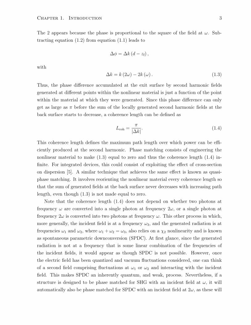
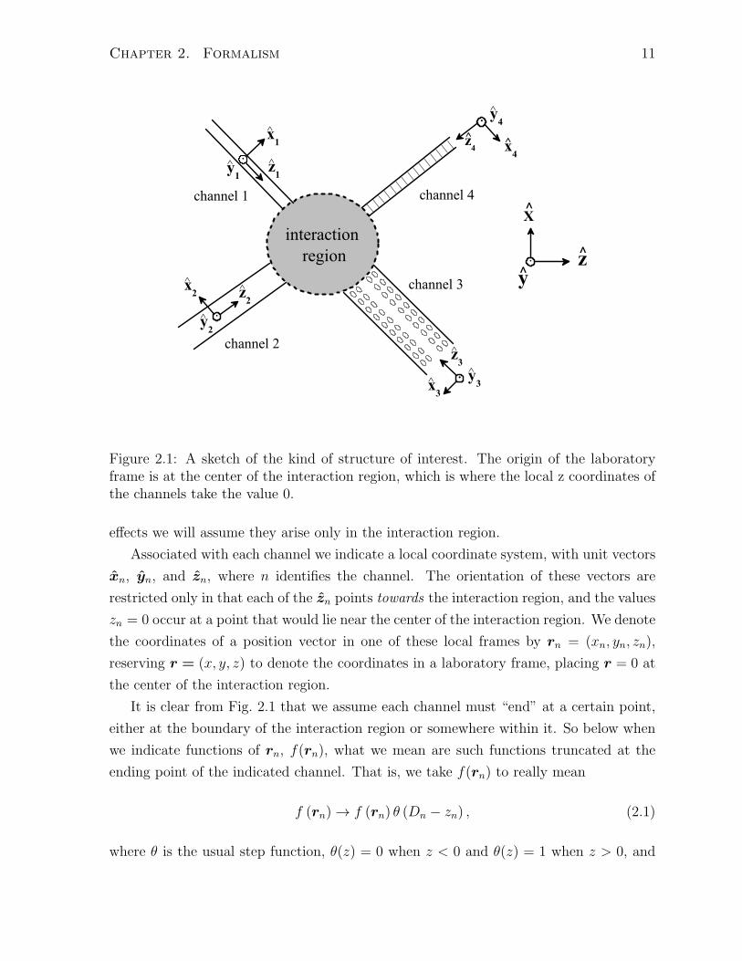
2.1 A sketch of the kind of structure of interest. The origin of the laboratory
frame is at the center of the interaction region, which is where the local z
coordinates of the channels take the value 0. . . . . . . . . . . . . . . . . 11
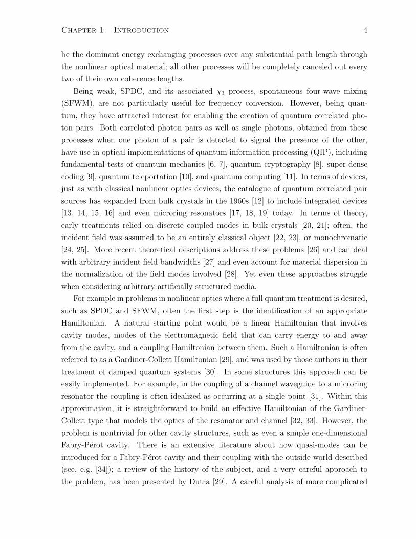
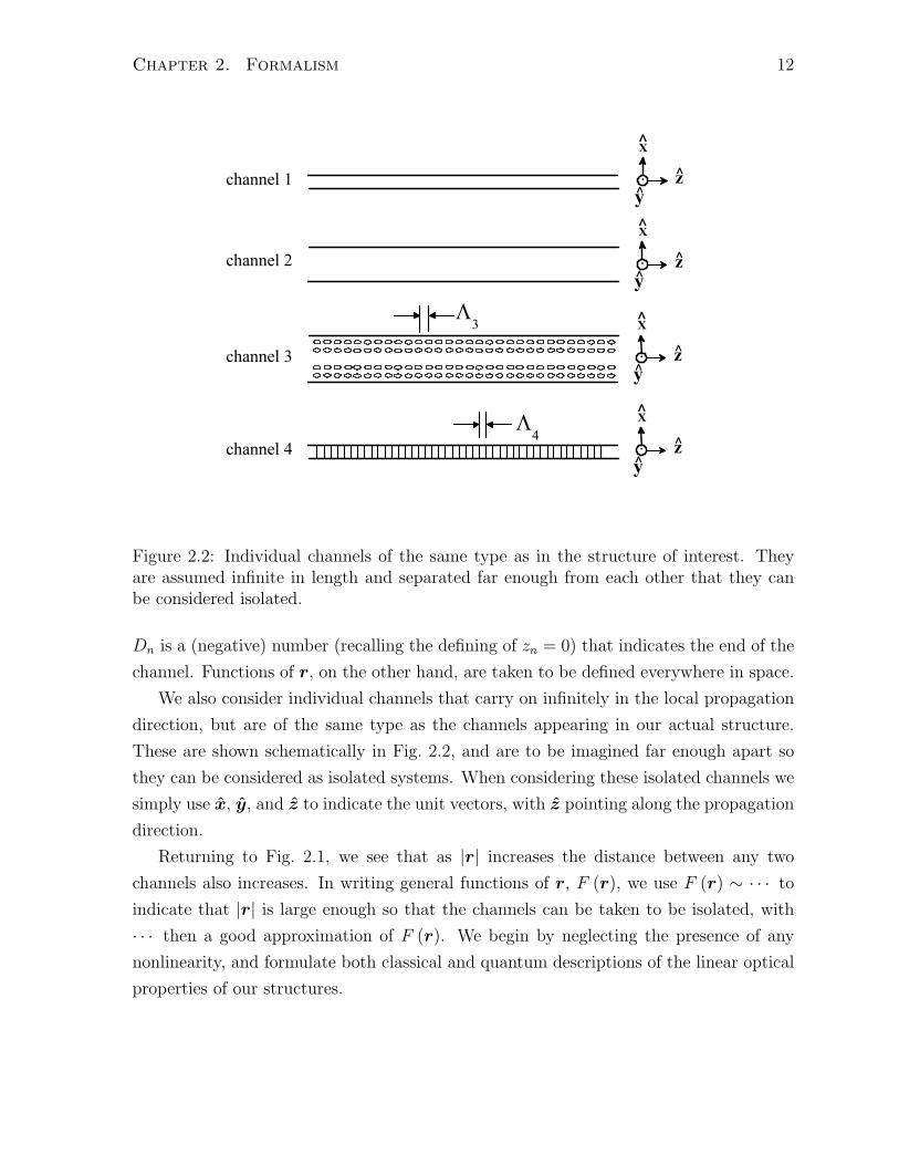
2.2 Individual channels of the same type as in the structure of interest. They
are assumed infinite in length and separated far enough from each other
that they can be considered isolated. . . . . . . . . . . . . . . . . . . . . 12
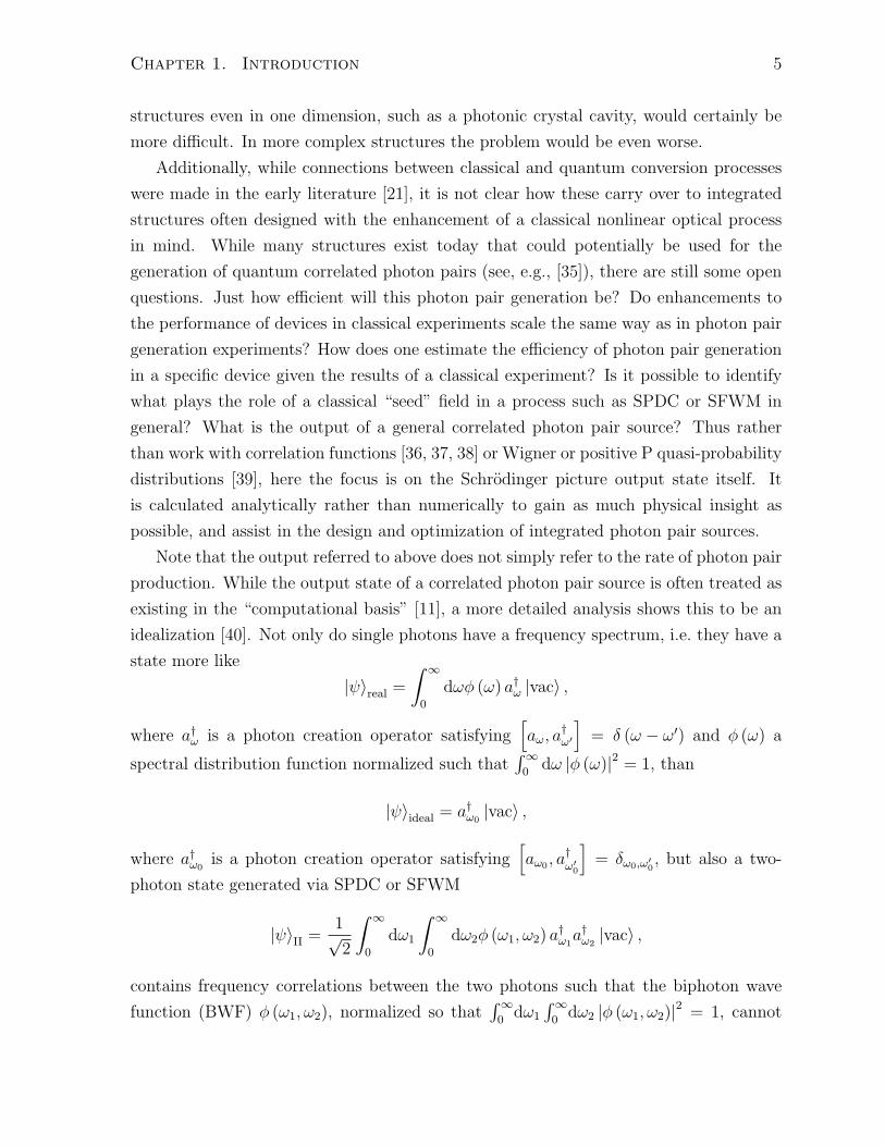
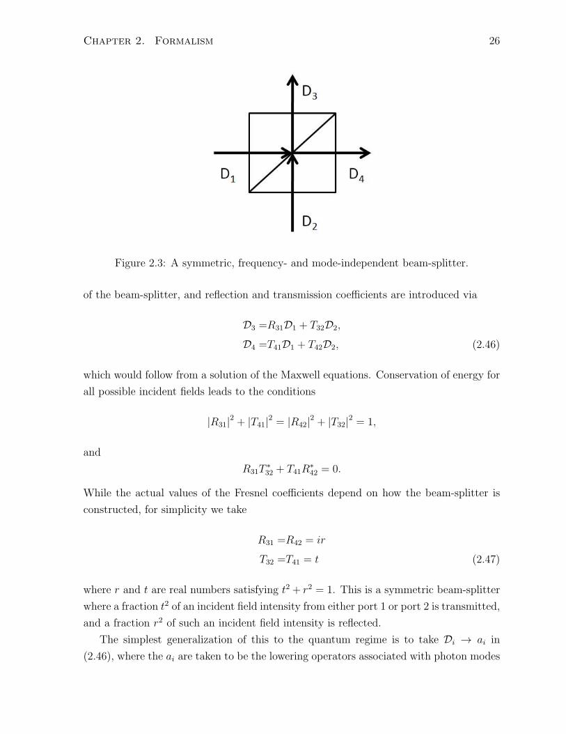
2.3 A symmetric, frequency- and mode-independent beam-splitter. . . . . . . 26
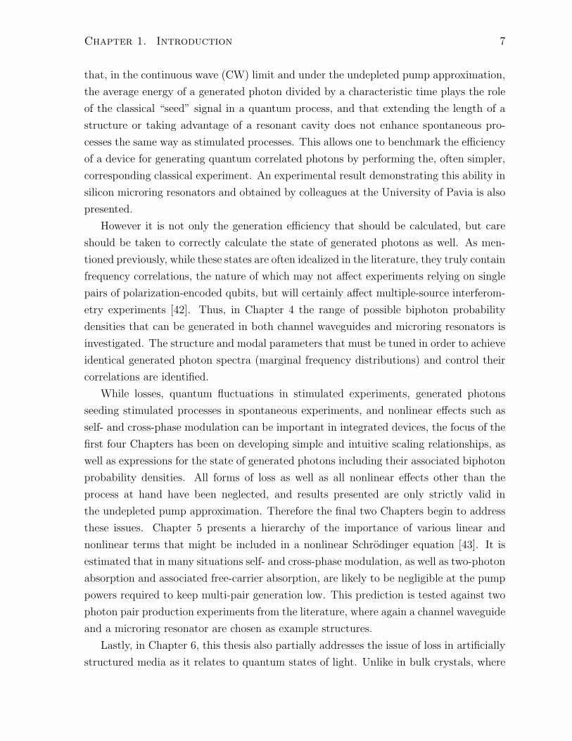
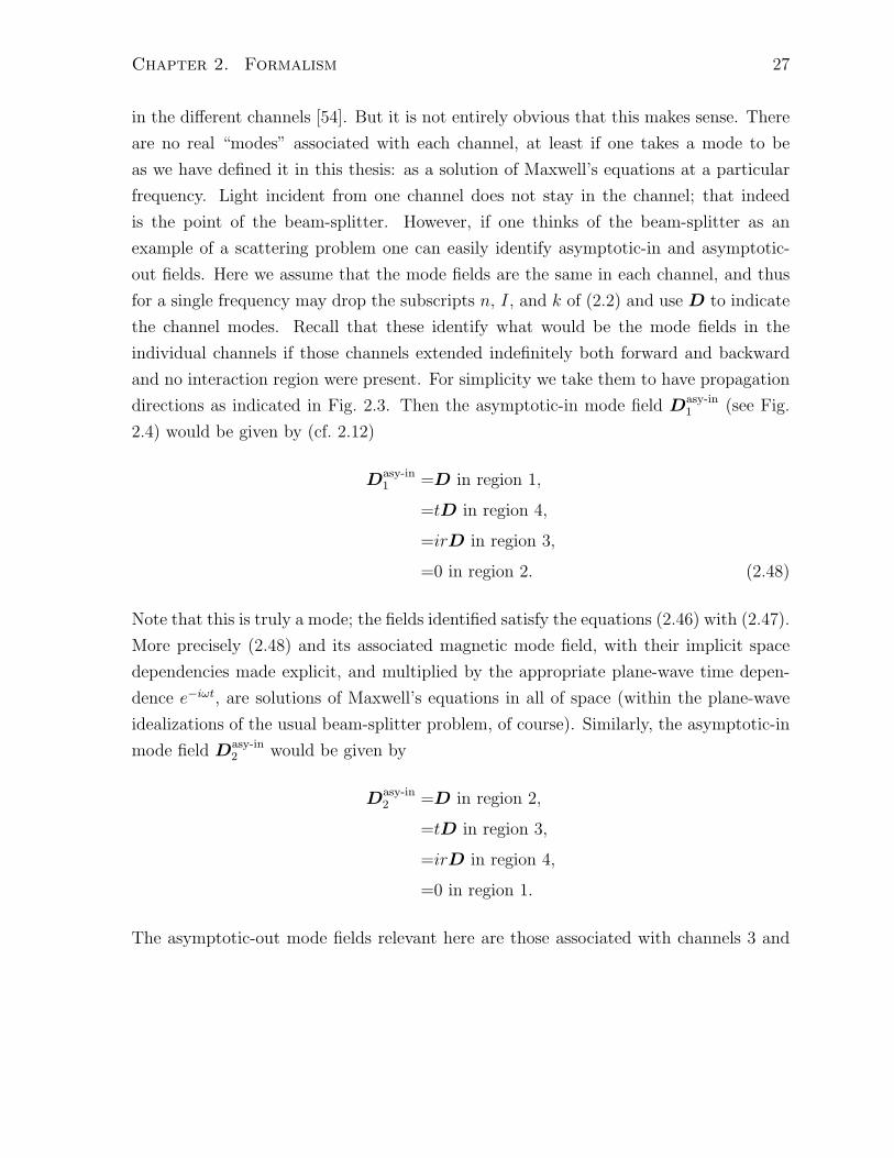
2.4 A beam-splitter described by asymptotic mode fields. . . . . . . . . . . . 29
3.1 Schematic of frequencies generated by second- and third-order nonlinear
optical processes, organized according to spontaneous, stimulated, and
reverse processes, with corresponding processes occupying the first two
columns. . . . . . . . . . . . . . . . . . . . . . . . . . . . . . . . . . . . . 40
3.2 Schematic of frequency spacings of second- and third-order nonlinear op-
tical processes. . . . . . . . . . . . . . . . . . . . . . . . . . . . . . . . . 41
3.3 Schematic of an effectively one-dimensional non-resonant structure. . . . 41
3.4 Schematic of a microring resonator side-coupled to a channel waveguide. 62
3.5 Transmission spectrum of the R = 5 µm ring. The inset shows a high-
resolution spectrum of the resonance at λ = 1558.5 nm. . . . . . . . . . . 71
3.6 (a) Example of a SFWM spectrum for a R = 5 µm ring resonator. (b)
Scaling of the estimated number of SFWM-generated signal (blue circles)
and idler (red triangles) photons inside the ring with varying PP, as well as
FWM-generated idler photons (black squares) with 47 µW injected at the
signal resonance. The black dashed line is the best fit to the FWM data
from Eq. (3.59) and the blue short dashed line is the theoretical prediction
from Eq. (3.60). . . . . . . . . . . . . . . . . . . . . . . . . . . . . . . . . 73
viii
3.7 (a) Scaling of the generated idler intensities with the ring radius, for FWM
and SFWM. The dashed lines are guides to the eye proportional to R−2.
(b) Ratio between the generated idler photons in SFWM and FWM ex-
periments performed using the same pump power [see Eq. (3.61)] for all
four rings investigated. The dashed line is given by Eq. (3.61). . . . . . . 74
4.1 Symmetry of a type-I BWF. We refer to the dashed red line as the 45
line, and the solid blue line as the pump line. . . . . . . . . . . . . . . . . 79
4.2 Theorist’s sketch of an entanglement swapping experiment. It is assumed
that at a polarization beam-splitter (PBS), vertically polarized photons
are reflected and horizontally polarized photons are transmitted. . . . . . 85
4.3 Sketch of potential pump waveform contributions to the SPDC biphoton
probability density (4.7). A representative pump pulse bandwidth ∆ω is
increased as panels move from left to right. . . . . . . . . . . . . . . . . . 87
4.4 Sketch of potential phase matching function contributions to the channel
SPDC biphoton probability density (4.8). A representative value of the
angle it makes with the horizontal θ (see (4.13)) is increased from 45 to
180 as panels move from left to right across the top row followed by the
bottom row. . . . . . . . . . . . . . . . . . . . . . . . . . . . . . . . . . . 89
4.5 Sketch of potential resonance function contributions to the microring ring
resonator SPDC biphoton probability density (4.9), for various resonance
linewidths. From left to right: ΩP ≈ Ωµ ≈ Ων ; ΩP ≫ Ωµ,Ων with Ωµ ≈ Ων ;
and ΩP ≫ Ωµ,Ων with Ωµ ≫ Ων . . . . . . . . . . . . . . . . . . . . . . . 90
6.1 Temporal evolution of the two-photon, single-photon, and vacuum contri-
bution to the lossy two-photon state. . . . . . . . . . . . . . . . . . . . . 117
ix
Chapter 1
Introduction
The field of nonlinear optics, first explored over 50 years ago [1], continues today to
see improvements in conversion efficiency and reductions in system size. Advances in
materials science research and fabrication techniques are moving bulk crystal experiments
onto a chip and into integrated commercial devices. Microring resonators, for instance,
have found use in signal processing and optical sensing, as classical frequency conversion
processes within them are well-understood [2, 3]. As with the move to integrated circuits
from vacuum tubes and discrete elements, microring resonators and other artificially
structured media allow for nonlinear optical applications to be realized more compactly
and requiring less power than with bulk crystal optics.
Such frequency conversion processes are possible because in general a nonlinear optical
material is capable of having an induced polarization P (r, t), and thus emitting radiation
[4], proportional to all incident fields as well as any power of each. A simple model that
illustrates this is
P i (r, t) =∑j
ε0χij1 (r)Ej (r, t) +
∑jk
ε0χijk2 (r)Ej (r, t)Ek (r, t)
+∑jkl
ε0χijkl3 (r)Ej (r, t)Ek (r, t)El (r, t) + · · · .
where ε0 is the permittivity of free space, χ1 (r) is the linear electric susceptibility, χ2 (r)
the second-order nonlinear electric susceptibility, χ3 (r) the third-order nonlinear electric
susceptibility, Ei (r, t) the ith component of the total electric field, and superscripts
indicate Cartesian components. The χ’s are taken to be real and, while they depend
on position and therefore allow the nonlinear optical material to be inhomogeneous, the
response is taken to be local in both time and space. That they are real and the response
is local implies that absorptive and dispersive effects, respectively, are negligible over the
1

Chapter 1. Introduction 2
frequency range of interest. From the viewpoint of an underlying microscopic theory, this
results when said frequency range is well below any resonant frequencies of the nonlinear
medium. As the total electric field can be composed of many incident fields, each at a
different frequency, the emitted radiation can be at any frequency nω1 +mω2 + ..., where
n and m are integers and ω1 and ω2 are the frequencies associated with the incident fields.
This allows for a multitude of possible energy exchanging processes involving incident
and generated fields.
Yet just because an energy exchanging process is possible in a material does not
automatically mean that it is efficient. The conversion efficiency of a given process
can be limited because the polarization induced by the incident field(s) is composed of
many local polarizations, which may or may not be radiating in phase. That is, fields
originating at different points within the material with the nonlinear electric susceptibility
will accumulate phase as they travel, which may add constructively or destructively at
the back or exit surface of the material. The technique of phase matching ensures that,
for at least one energy exchanging process, the sum of these fields at the back surface
only increases with increasing path length through the nonlinear optical material. Thus,
over substantial path lengths, phase matching can determine which energy exchanging
processes are most efficient, as all others will have sums of locally generated fields that
at some point decrease with increasing path length.
By way of example, consider the process of second harmonic generation (SHG) in a
uniform medium. In this process, there is one incident field, only a second order nonlinear
electric susceptibility, χ2, is required, and the generated radiation is at twice the frequency
of the incident field, also known as the second harmonic. Note that this process is not
possible in a material that has a center of inversion, as symmetry arguments show that
the only possible χ2 for such a material is one that is equal to zero. For simplicity, assume
a dispersive material, i.e. one where k(2ω) = 2k(ω), with a non-zero χ2, and take the
propagation to be entirely in the z direction. Then the phase, ϕ, accumulated at the
back surface, z = zb, by a field generated at the front or entrance surface, z = zf, can be
expressed as
ϕzf (zb) = k (2ω) (zb − zf) = k (2ω) (d− zf) + k (2ω) (zb − d) . (1.1)
Similarly, the phase accumulated at the back surface by a field generated at some point,
z = d, between the front and back surfaces can be expressed as
ϕd (zb) = 2k (ω) (d− zf) + k (2ω) (zb − d) . (1.2)
Chapter 1. Introduction 3
The 2 appears because the phase is proportional to the square of the field at ω. Sub-
tracting equation (1.2) from equation (1.1) leads to
∆ϕ = ∆k (d− zf) ,
with
∆k = k (2ω) − 2k (ω) . (1.3)
Thus, the phase difference accumulated at the exit surface by second harmonic fields
generated at different points within the nonlinear material is just a function of the point
within the material at which they were generated. Since this phase difference can only
get as large as π before the sum of the locally generated second harmonic fields at the
back surface starts to decrease, a coherence length can be defined as
Lcoh =π
|∆k|. (1.4)
This coherence length defines the maximum path length over which power can be effi-
ciently produced at the second harmonic. Phase matching consists of engineering the
nonlinear material to make (1.3) equal to zero and thus the coherence length (1.4) in-
finite. For integrated devices, this could consist of exploiting the effect of cross-section
on dispersion [5]. A similar technique that achieves the same effect is known as quasi-
phase matching. It involves reorienting the nonlinear material every coherence length so
that the sum of generated fields at the back surface never decreases with increasing path
length, even though (1.3) is not made equal to zero.
Note that the coherence length (1.4) does not depend on whether two photons at
frequency ω are converted into a single photon at frequency 2ω, or a single photon at
frequency 2ω is converted into two photons at frequency ω. This other process in which,
more generally, the incident field is at a frequency ω3, and the generated radiation is at
frequencies ω1 and ω2, where ω1 + ω2 = ω3, also relies on a χ2 nonlinearity and is known
as spontaneous parametric downconversion (SPDC). At first glance, since the generated
radiation is not at a frequency that is some linear combination of the frequencies of
the incident fields, it would appear as though SPDC is not possible. However, once
the electric field has been quantized and vacuum fluctuations considered, one can think
of a second field comprising fluctuations at ω1 or ω2 and interacting with the incident
field. This makes SPDC an inherently quantum, and weak, process. Nevertheless, if a
structure is designed to be phase matched for SHG with an incident field at ω, it will
automatically also be phase matched for SPDC with an incident field at 2ω, as these will
Chapter 1. Introduction 4
be the dominant energy exchanging processes over any substantial path length through
the nonlinear optical material; all other processes will be completely canceled out every
two of their own coherence lengths.
Being weak, SPDC, and its associated χ3 process, spontaneous four-wave mixing
(SFWM), are not particularly useful for frequency conversion. However, being quan-
tum, they have attracted interest for enabling the creation of quantum correlated pho-
ton pairs. Both correlated photon pairs as well as single photons, obtained from these
processes when one photon of a pair is detected to signal the presence of the other,
have use in optical implementations of quantum information processing (QIP), including
fundamental tests of quantum mechanics [6, 7], quantum cryptography [8], super-dense
coding [9], quantum teleportation [10], and quantum computing [11]. In terms of devices,
just as with classical nonlinear optics devices, the catalogue of quantum correlated pair
sources has expanded from bulk crystals in the 1960s [12] to include integrated devices
[13, 14, 15, 16] and even microring resonators [17, 18, 19] today. In terms of theory,
early treatments relied on discrete coupled modes in bulk crystals [20, 21]; often, the
incident field was assumed to be an entirely classical object [22, 23], or monochromatic
[24, 25]. More recent theoretical descriptions address these problems [26] and can deal
with arbitrary incident field bandwidths [27] and even account for material dispersion in
the normalization of the field modes involved [28]. Yet even these approaches struggle
when considering arbitrary artificially structured media.
For example in problems in nonlinear optics where a full quantum treatment is desired,
such as SPDC and SFWM, often the first step is the identification of an appropriate
Hamiltonian. A natural starting point would be a linear Hamiltonian that involves
cavity modes, modes of the electromagnetic field that can carry energy to and away
from the cavity, and a coupling Hamiltonian between them. Such a Hamiltonian is often
referred to as a Gardiner-Collett Hamiltonian [29], and was used by those authors in their
treatment of damped quantum systems [30]. In some structures this approach can be
easily implemented. For example, in the coupling of a channel waveguide to a microring
resonator the coupling is often idealized as occurring at a single point [31]. Within this
approximation, it is straightforward to build an effective Hamiltonian of the Gardiner-
Collett type that models the optics of the resonator and channel [32, 33]. However, the
problem is nontrivial for other cavity structures, such as even a simple one-dimensional
Fabry-Perot cavity. There is an extensive literature about how quasi-modes can be
introduced for a Fabry-Perot cavity and their coupling with the outside world described
(see, e.g. [34]); a review of the history of the subject, and a very careful approach to
the problem, has been presented by Dutra [29]. A careful analysis of more complicated
Chapter 1. Introduction 5
structures even in one dimension, such as a photonic crystal cavity, would certainly be
more difficult. In more complex structures the problem would be even worse.
Additionally, while connections between classical and quantum conversion processes
were made in the early literature [21], it is not clear how these carry over to integrated
structures often designed with the enhancement of a classical nonlinear optical process
in mind. While many structures exist today that could potentially be used for the
generation of quantum correlated photon pairs (see, e.g., [35]), there are still some open
questions. Just how efficient will this photon pair generation be? Do enhancements to
the performance of devices in classical experiments scale the same way as in photon pair
generation experiments? How does one estimate the efficiency of photon pair generation
in a specific device given the results of a classical experiment? Is it possible to identify
what plays the role of a classical “seed” field in a process such as SPDC or SFWM in
general? What is the output of a general correlated photon pair source? Thus rather
than work with correlation functions [36, 37, 38] or Wigner or positive P quasi-probability
distributions [39], here the focus is on the Schrodinger picture output state itself. It
is calculated analytically rather than numerically to gain as much physical insight as
possible, and assist in the design and optimization of integrated photon pair sources.
Note that the output referred to above does not simply refer to the rate of photon pair
production. While the output state of a correlated photon pair source is often treated as
existing in the “computational basis” [11], a more detailed analysis shows this to be an
idealization [40]. Not only do single photons have a frequency spectrum, i.e. they have a
state more like
|ψ⟩real =
∫ ∞
0
dωϕ (ω) a†ω |vac⟩ ,
where a†ω is a photon creation operator satisfying[aω, a
†ω′
]= δ (ω − ω′) and ϕ (ω) a
spectral distribution function normalized such that∫∞0
dω |ϕ (ω)|2 = 1, than
|ψ⟩ideal = a†ω0|vac⟩ ,
where a†ω0is a photon creation operator satisfying
[aω0 , a
†ω′0
]= δω0,ω′
0, but also a two-
photon state generated via SPDC or SFWM
|ψ⟩II =1√2
∫ ∞
0
dω1
∫ ∞
0
dω2ϕ (ω1, ω2) a†ω1a†ω2
|vac⟩ ,
contains frequency correlations between the two photons such that the biphoton wave
function (BWF) ϕ (ω1, ω2), normalized so that∫∞0
dω1
∫∞0
dω2 |ϕ (ω1, ω2)|2 = 1, cannot

Chapter 1. Introduction 6
be factored into a product of a function of ω1 and a function of ω2, i.e. ϕ (ω1, ω2) =f (ω1) f (ω2). These issues become quite important when interacting single photons with
e.g. quantum memories [41] and interfering photons produced from multiple sources [42],
respectively. However as there is more freedom in the design of artificially structured
media than bulk crystals, there is also more freedom over the exact form the BWF, and
thus the biphoton probability density |ϕ (ω1, ω2)|2, that they produce takes compared to
bulk crystals.
In short, the move from bulk crystal optics to integrated devices has brought with it
a number of theoretical challenges and questions. There is a need for theoretical tools
that can calculate the output of a wide range of correlated photon pair sources, allowing
for easy comparison of the utility of various sources for varied applications as well as the
optimization of proposed sources for specific applications before development is started.
This thesis presents and applies just that, and is organized as follows.
In Chapter 2 a general Hamiltonian formalism that places quantum and classical wave
mixing processes on equal theoretical footing is presented. It correctly accounts for mate-
rial and modal dispersion in the normalization of the linear modes of the system, and can
easily be applied to integrated nonlinear structures. Building upon the backward Heisen-
berg picture approach of Yang et al. [28], it leverages the solutions of linear scattering
problems to attack nonlinear scattering problems, allowing the consideration of complex
cavity structures without the need to construct a Hamiltonian for the cavity modes or for
coupling between cavity modes and propagating modes. Indeed, this approach makes it
very simple to identify the physics of all of the interactions of the fields involved, whether
classical or quantum, as well as all approximations involved in a given calculation. This
is made possible by taking advantage of the fact that, to first approximation, one expects
the output state from a given device to consist of an undepleted pump as well as the
state of generated photons; calculating the evolution of the undepleted pump, which is
often quite simple, and pulling it aside implies that what remains in the output state
must be the generated photons of interest.
In Chapter 3 the formalism is applied to two specific structure types, both when a
second-order nonlinearity is dominant and when a third-order nonlinearity is dominant,
to answer questions relating to pair generation efficiency, enhancement, and scaling. The
formalism introduced in the previous Chapter enables general expressions for the output
state to be written down regardless of the source, and comparisons between the genera-
tion efficiencies of SPDC and difference frequency generation (DFG) or SHG, as well as
between those of SFWM and classical four-wave mixing (FWM), in both channel waveg-
uides and microring resonator structures are made as examples. In all cases it is shown
Chapter 1. Introduction 7
that, in the continuous wave (CW) limit and under the undepleted pump approximation,
the average energy of a generated photon divided by a characteristic time plays the role
of the classical “seed” signal in a quantum process, and that extending the length of a
structure or taking advantage of a resonant cavity does not enhance spontaneous pro-
cesses the same way as stimulated processes. This allows one to benchmark the efficiency
of a device for generating quantum correlated photons by performing the, often simpler,
corresponding classical experiment. An experimental result demonstrating this ability in
silicon microring resonators and obtained by colleagues at the University of Pavia is also
presented.
However it is not only the generation efficiency that should be calculated, but care
should be taken to correctly calculate the state of generated photons as well. As men-
tioned previously, while these states are often idealized in the literature, they truly contain
frequency correlations, the nature of which may not affect experiments relying on single
pairs of polarization-encoded qubits, but will certainly affect multiple-source interferom-
etry experiments [42]. Thus, in Chapter 4 the range of possible biphoton probability
densities that can be generated in both channel waveguides and microring resonators is
investigated. The structure and modal parameters that must be tuned in order to achieve
identical generated photon spectra (marginal frequency distributions) and control their
correlations are identified.
While losses, quantum fluctuations in stimulated experiments, generated photons
seeding stimulated processes in spontaneous experiments, and nonlinear effects such as
self- and cross-phase modulation can be important in integrated devices, the focus of the
first four Chapters has been on developing simple and intuitive scaling relationships, as
well as expressions for the state of generated photons including their associated biphoton
probability densities. All forms of loss as well as all nonlinear effects other than the
process at hand have been neglected, and results presented are only strictly valid in
the undepleted pump approximation. Therefore the final two Chapters begin to address
these issues. Chapter 5 presents a hierarchy of the importance of various linear and
nonlinear terms that might be included in a nonlinear Schrodinger equation [43]. It is
estimated that in many situations self- and cross-phase modulation, as well as two-photon
absorption and associated free-carrier absorption, are likely to be negligible at the pump
powers required to keep multi-pair generation low. This prediction is tested against two
photon pair production experiments from the literature, where again a channel waveguide
and a microring resonator are chosen as example structures.
Lastly, in Chapter 6, this thesis also partially addresses the issue of loss in artificially
structured media as it relates to quantum states of light. Unlike in bulk crystals, where
Chapter 1. Introduction 8
usually coupling and absorption losses are the most relevant losses, the dominant loss
in integrated devices is often scattering loss due to sidewall roughness from fabrication
imperfections. Hamiltonians for systems of statistically independent reservoirs and the
coupling of waveguide modes to them are introduced, and quantum Langevin equations
are solved, with the reservoir modes eventually traced over, to calculate the propagation
of a coherent state, two-photon state, and squeezed-vacuum state in the presence of
scattering loss, while preserving the necessary canonical equal-time bosonic commutation
relations as the system evolves.
The seventh and eighth paragraphs of this introduction are published in [44] and
[45] respectively. Chapter 2 contains excerpts from M. Liscidini, L. G. Helt, and J.
E. Sipe, ”Asymptotic fields for a Hamiltonian treatment of nonlinear electromagnetic
phenomena,” Phys. Rev. A, 85(1):013833, (2012). Copyright (2012) by the American
Physical Society. Additionally, the first two Sections of Chapter 3 are published in [45]
(albeit with a slightly different calculation method) and the experimental Section (3.3)
of Chapter 3 is adapted from [18].
Chapter 2
Formalism
In this Chapter I introduce the formalism upon which much of this thesis is based. It
is a Hamiltonian formalism for which the field dynamics and normalization condition
are well-known [46], but it leverages classical asymptotic-in and asymptotic-out fields
to expand the magnetic and electric displacement fields and field operators into sets of
modes that are useful for describing both classical and quantum nonlinear optics problems
in artificially structured media. These fields are the stationary solutions of the classical
linear Maxwell equations, and can be evaluated analytically or numerically.
This strategy avoids the introduction of artificial “cavity modes,” which of course do
not truly exist in e.g. a microring resonator or photonic crystal structure, as well as their
coupling to input/output channels; the enhancement of nonlinear optical effects due to
the time light spends in a cavity-like structure is completely captured by the distribution
of the asymptotic-in and asymptotic-out fields. Further, in photon generation problems
the formalism takes advantage of the fact that, in the perturbative limit, the output state
is expected to consist of an undepleted pump as well as the state of generated photons.
This enables the state of the pump to be isolated and pulled aside, for its evolution is
well-known and can be easily calculated [43], and allows identification of the remainder of
the output state with the state of generated photons. Performing this isolation before the
output state is calculated avoids the need to separate the (potentially non-commuting)
operators of the pump and generated fields with Baker-Campbell-Hausdorff relations [47],
and thus makes the physics of both the pump and generated photons more transparent.
While earlier work has anticipated some aspects of what is presented here in optics
[48, 49], and analogous approaches have arisen in the treatment of electron transport in
channels and cavity-like structures (see, e.g. [50]), here a general framework for problems
in nonlinear quantum optics is developed. The formalism can consider single-particle
states, as in elementary quantum scattering theory, as well as more complicated states
9
Chapter 2. Formalism 10
including coherent states, squeezed vacua, and Fock states. Additionally, both the ma-
terial and modal dispersion of the input and output channels, such as those sketched in
Fig. 2.1, can be important in the analysis of real artificially structured materials; this
approach can include them very naturally.
2.1 Asymptotic-In and -Out Fields
The asymptotic-in/-out field (operator) expansion harks back to the elementary scatter-
ing theory in quantum mechanics. There one can introduce asymptotic-in and asymptotic-
out states, as done in the classic paper of Breit and Bethe [51]. These are full solutions
of the (linear) Schrodinger equation, including the scattering potential, and exist every-
where in space. But they are built so that a superposition of them corresponds to an
incident wave packet at t = −∞ (asymptotic-in), or an exiting wave packet at t = ∞(asymptotic-out) [52]. In elementary quantum mechanics the construction of these states
constitutes a solution of the scattering problem itself. In photonics the construction of
the corresponding solutions of the linear Maxwell equations for a structure such as that
in Fig. 2.1, which can often be found numerically even if not analytically, constitutes a
solution of only the linear scattering problem. Indeed, as we show in detail below, that
linear scattering problem can be encapsulated in a transformation from the asymptotic-in
to the asymptotic-out fields. However, those fields also form the natural basis for the
treatment of a nonlinear optics problem, especially if the nonlinearity can be idealized
as restricted to an “interaction” region as indicated schematically in Fig. 2.1; in the par-
ticular example of a microring resonator side-coupled to a channel waveguide this would
correspond to the ring itself.
2.1.1 Structures of Interest
We consider structures of the form indicated schematically in Fig. 2.1, where there are a
number of channels connected by an interaction region. The channels could all be of the
same type, or of different types, as indicated in the figure. However, it will be useful to
adopt the language appropriate for the kinds of channels sketched in Fig. 2.1 to fix the
notation. The only really important assumption is that these channels identify all the
ways that energy can move towards or away from the interaction region, i.e. all pathways
of any significance are taken into account, neglecting absorption and scattering losses for
now. We leave the details of the interaction region, indicated only in “cartoon fashion”
by the central circular region, unspecified for the moment. When we include nonlinear
Chapter 2. Formalism 11
yz
^^.
X
channel 2
channel 3
channel 4
y4^
^
interaction region
.
x4^z
4.y1^
x1^
z1^
y2^
x2^
z2^
y3^
z3^
x3^ .
channel 1
.
Figure 2.1: A sketch of the kind of structure of interest. The origin of the laboratoryframe is at the center of the interaction region, which is where the local z coordinates ofthe channels take the value 0.
effects we will assume they arise only in the interaction region.
Associated with each channel we indicate a local coordinate system, with unit vectors
xn, yn, and zn, where n identifies the channel. The orientation of these vectors are
restricted only in that each of the zn points towards the interaction region, and the values
zn = 0 occur at a point that would lie near the center of the interaction region. We denote
the coordinates of a position vector in one of these local frames by rn = (xn, yn, zn),
reserving r = (x, y, z) to denote the coordinates in a laboratory frame, placing r = 0 at
the center of the interaction region.
It is clear from Fig. 2.1 that we assume each channel must “end” at a certain point,
either at the boundary of the interaction region or somewhere within it. So below when
we indicate functions of rn, f(rn), what we mean are such functions truncated at the
ending point of the indicated channel. That is, we take f(rn) to really mean
f (rn) → f (rn) θ (Dn − zn) , (2.1)
where θ is the usual step function, θ(z) = 0 when z < 0 and θ(z) = 1 when z > 0, and
Chapter 2. Formalism 12
yz
^^.
X
yz
^^.
X
yz
^^.
X
channel 1
channel 2
channel 3
channel 4
yz
^^.
X
Figure 2.2: Individual channels of the same type as in the structure of interest. Theyare assumed infinite in length and separated far enough from each other that they canbe considered isolated.
Dn is a (negative) number (recalling the defining of zn = 0) that indicates the end of the
channel. Functions of r, on the other hand, are taken to be defined everywhere in space.
We also consider individual channels that carry on infinitely in the local propagation
direction, but are of the same type as the channels appearing in our actual structure.
These are shown schematically in Fig. 2.2, and are to be imagined far enough apart so
they can be considered as isolated systems. When considering these isolated channels we
simply use x, y, and z to indicate the unit vectors, with z pointing along the propagation
direction.
Returning to Fig. 2.1, we see that as |r| increases the distance between any two
channels also increases. In writing general functions of r, F (r), we use F (r) ∼ · · · to
indicate that |r| is large enough so that the channels can be taken to be isolated, with
· · · then a good approximation of F (r). We begin by neglecting the presence of any
nonlinearity, and formulate both classical and quantum descriptions of the linear optical
properties of our structures.

Chapter 2. Formalism 13
2.1.2 Classical Formulation
A starting point for our calculations will be the classical optics of the isolated channels
sketched in Fig. 2.2. Since the displacement field D (r, t) and the magnetic field B (r, t)
are divergenceless, it is useful to consider them as our fundamental fields. The fields
E (r, t) and H (r, t) are then taken as derived fields, and our constitutive relations are
strictly taken as conditions that relate E (r, t) and H (r, t) to D (r, t) and B (r, t).
Within such a framework the Maxwell equations ∂B (r, t) /∂t = −∇ × E (r, t) and
∂D (r, t) /∂t = ∇×H (r, t) guarantee that if D (r, t) and B (r, t) are set divergenceless
as an initial condition then they will remain so. Alternately, if we seek stationary fields
D (r, t) = DnIk (r) e−iωnIkt + c.c.,
B (r, t) = BnIk (r) e−iωnIkt + c.c., (2.2)
where c.c. stands for complex conjugation, those same Maxwell equations guarantee
that D (r, t) and B (r, t) are divergenceless. Our notation is motivated by the fact that
these fields are simply the propagation modes (e.g. “lowest-order TE-like mode” of a ridge
waveguide or “first TM-band” of a photonic crystal), I, of the channels, n, for given wave
number dependent frequencies ωnIk > 0. They can be found starting from the equations
for the time derivatives, along with linear constitutive relations. Neglecting magnetic
effects and taking the medium to be isotropic, for stationary fields the constitutive rela-
tions are of the form HnIk (r) = µ−10 BnIk (r) and EnIk (r) = ϵ−1
0 n−2 (r;ωnIk)DnIk (r),
where ϵ0n2 (r;ωnIk) is the dielectric constant at the frequency ωnIk to be determined.
These lead to time-independent Maxwell equations for the displacement and magnetic
mode fields
∇×[
DnIk (r)
n2 (r;ωnIk)
]= iε0ωnIkBnIk (r) ,
∇×BnIk (r) = −iµ0ωnIkDnIk (r) . (2.3)
which can then be combined into a Hermitian eigenvalue problem or so-called “Master
equation”
∇×[∇×BnIk (r)
n2 (r;ωnIk)
]=ω2nIk
c2BnIk (r) , (2.4)
for ωnIk = 0 subject to the divergence condition ∇ ·BnIk (r) = 0; the DnIk (r) can then
be found from the BnIk (r) using the second of (2.3). In practice, (2.4) can be solved
using FDTD, local eigensolver, or iterative methods. We can then expand the full fields
Chapter 2. Formalism 14
for a set of isolated channels as shown in Fig. 2.1 according to
D (r, t) =∑
n,I∈σn
∫ ∞
−∞dk γnIke
−iωnIktDnIk (r) + c.c.,
B (r, t) =∑
n,I∈σn
∫ ∞
−∞dk γnIke
−iωnIktBnIk (r) + c.c., (2.5)
with complex mode amplitudes γnIk; the set of modes allowed in channel n is specified
by σn. Here we are only interested in modes confined to the structure, and in general
only over a certain frequency range, and so the integral range from −∞ to ∞ in (2.5)
is schematic; in general there will be mode cut-offs, and if the waveguide structure has
periodicity in the z direction the range of k will at most be the first Brillouin zone. To
take into account possible periodicity along the z direction of the structure we write
DnIk (r) =dnIk (r)√
2πeikz,
BnIk (r) =bnIk (r)√
2πeikz, (2.6)
where the functions dnIk (r) and bnIk (r) are periodic in the z direction with the period-
icity, Λn, of the structure,
dnIk (r) = dnIk (r + Λnz) , (2.7)
bnIk (r) = bnIk (r + Λnz) . (2.8)
We assume no significant absorption or scattering losses in the frequency range of interest,
but material dispersion is taken into account by the normalization condition [46]
1
Λn
∫V
d3rd∗nIk (r) · dnIk (r)
ε0n2 (r;ωnIk)
vp (r;ωnIk)
vg (r;ωnIk)= 1, (2.9)
where vp and vg are group and phase velocities, respectively, and the integration is per-
formed over a volume V corresponding to the entire (x, y) plane as well as a single period
Λn along the z axis. This condition is obtained from consideration of the full polari-
ton modes of the system, including electromagnetic and medium components. While
the medium component can be found from the electromagnetic component and the re-
sponse of the system n (r;ωnIk) [46], for our purposes it suffices to concentrate on the
electromagnetic component. Note that while the full polariton modes form a complete
orthonormal set, their electromagnetic component need not be orthogonal. The solutions

Chapter 2. Formalism 15
at k and −k are not independent, and the relation between them can be fixed by taking
DnI(−k) (r) = D∗nIk (r) ,
BnI(−k) (r) = −B∗nIk (r) . (2.10)
We return to Fig. 2.1 now, and look for solutions of the classical Maxwell equations
for this structure that oscillate at frequency ωnIk and have mode fields of the form
Dasy-innIk (r) = DnIk (rn) + Dout
nIk (r) ,
Basy-innIk (r) = BnIk (rn) + Bout
nIk (r) , (2.11)
for positive k, where the “out” superscript indicates that far from the interaction re-
gion DoutnIk(r) and Bout
nIk(r) consist of “out-going” waves, i.e. waves traveling in the −zn
direction, in each channel. We write this as
Dasy-innIk (r) ∼ DnIk (rn) +
∑n′,I′∈σn′
∫ ∞
0
dk′ T outnI;n′I′ (k, k′)Dn′I′(−k′) (rn′) , (2.12)
for positive k. We refer to(Dasy-in
nIk (r) ,Basy-innIk (r)
)as an asymptotic-in mode field. Re-
call from above that the tilde indicates that the right hand side of (2.12) is only a valid
approximation to Dasy-innIk (r) in the asymptotic regime, i.e. for large |r|. For an interac-
tion region with dimensions on the order of tens of wavelengths of a given asymptotic
mode field, the asymptotic regime generally corresponds to at least several thousands of
wavelengths from the interaction region. This is indeed true for a cavity structure, where
the fields within a few wavelengths of the cavity have a more complicated form than in
(2.12). However, it should be noted that in some cases this regime may be relaxed. For
some effectively one-dimensional structures, for which there is only one output channel
directly in line with the input channel, such as a planar one-dimensional photonic crys-
tal, it may be relaxed all the way to the edge of the interaction region itself [44]. Of
more importance is that in practice sources and detectors are placed far enough from the
interaction region to be in the asymptotic regime, and so it is photons corresponding to
the fields on right hand side of (2.12) that are created and/or detected.
In expressions like (2.12) when coordinates such as rn appear on the right hand side
of the equation, the implication is that they should be evaluated at the physical point
corresponding to the coordinates r in the laboratory frame appearing on the left hand side
of the equation (but recall (2.1)). Since this mode field corresponds to a field oscillating
at frequency ωnIk, the only k′ for which T outnI;n′I′ (k, k′) can be non-vanishing are those for
Chapter 2. Formalism 16
which ωn′I′k′ = ωnIk for positive k and k′. If we denote by snI;n′I′ (k) the positive value
of k′ for which indeed ωn′I′k′ = ωnIk holds for each given k, then T outnI;n′I′ (k, k′) must be
of the form
T outnI;n′I′ (k, k′) = τ outnI;n′I′ (k) δ (k′ − snI;n′I′ (k)) , (2.13)
where the Dirac delta function provides the restriction.
The form of τ outnI;n′I′(k) is of course determined by the interaction region, but the
physics of (2.12) is clear. Far from the interaction region, the exact solution Dasy-innIk (r)
of Maxwell’s equations corresponds to a wave “in-coming” in mode I of channel n, and
“out-going” waves in general in all modes of all channels. Thus these asymptotic-in mode
fields are analogous to the asymptotic-in states that appear in the elementary quantum
theory of scattering [51]. They share with them an important feature, which we now
recall.
Suppose that we construct a superposition of asymptotic-in mode fields of the form
D (r, t) =∑
n,I∈σn
∫ ∞
0
dk αnIke−iωnIktDasy-in
nIk (r) + c.c.,
B (r, t) =∑
n,I∈σn
∫ ∞
0
dk αnIke−iωnIktBasy-in
nIk (r) + c.c. (2.14)
Choosing the complex amplitudes αnIk such that, were we to put γnIk = αnIk for k > 0
and vanishing otherwise in (2.5), we would have field profiles propagating in the +zn
direction in each channel and, at t = 0, the field profiles would be centered at zn = 0; at
t0 ≪ 0, they would correspond to field profiles centered at zn ≪ 0. Following arguments
in [51], as t→ −∞ the fields (D (r, t) ,B (r, t)) of (2.14) can be written in the simplified
form
D (r, t) →∑
n,I∈σn
∫ ∞
0
dk αnIke−iωnIktDnIk (rn) + c.c.,
B (r, t) →∑
n,I∈σn
∫ ∞
0
dk αnIke−iωnIktBnIk (rn) + c.c. (2.15)
That is, we have field profiles incident on the interaction region from the different chan-
nels; at such an early time the fields DoutnIk (r) and Bout
nIk (r) in (2.11) can be neglected,
not because they are small, but because they are added together with different phases in
(2.14) for different k such that their net contribution vanishes. As t → ∞, on the other
hand, when with our choice of γnIk in (2.5) the field profiles would be centered at zn ≫ 0,
only the DoutnIk (r) and Bout
nIk (r) in the asymptotic-in mode fields will make a contribution

Chapter 2. Formalism 17
to (2.14). Indeed, the only regions of rn for which the part of the field arising from the
superposition of the DnIk (rn) and BnIk (rn) would make a contribution correspond to
the region Dn > zn in the notation of (2.1), and thus do not correspond to regions in
the physical structure. Thus for t → ∞ there are only out-going field profiles in each
channel.
Such a superposition (2.14), with the amplitudes αnIk properly chosen, corresponds to
a scattering experiment with fields incident in general from each channel, as described by
(2.15). Two important consequences follow from this. The first is that the asymptotic-in
mode fields can be calculated numerically, even if they cannot be found or reasonably
modeled analytically. The second is that since the asymptotic-in mode fields can be used
to model all scattering experiments, they can be used to describe all electromagnetic
fields of the system, as long as there are no modes of the electromagnetic field completely
bound to the interaction region. And so (2.14) can be taken as an expansion of all
electromagnetic fields of interest.
Similarly we can introduce asymptotic-out mode fields: full solutions of the Maxwell
equations labeled by positive k and of the form
Dasy-outnIk (r) = DnI(−k) (rn) + Din
nIk (r) ,
Basy-outnIk (r) = BnI(−k) (rn) + Bin
nIk (r) , (2.16)
where the “in” superscript indicates that far from the interaction region DinnIk(r) and
BinnIk(r) consist of “in-coming” waves, i.e. waves traveling in the +zn direction, in each
channel. We write this as
Dasy-outnIk (r) ∼ DnI(−k) (rn) +
∑n′,I′∈σn′
∫ ∞
0
dk′ T innI;n′I′ (k, k′)Dn′I′k′ (rn′) , (2.17)
and, again using the fact that this field must be oscillating at frequency ωnI(−k) = ωnIk,
the coefficient T innI;n′I′ (k, k′) must be of the form
T innI;n′I′ (k, k′) = τ innI;n′I′ (k) δ (k′ − snI;n′I′ (k)) .
We can identify the physics of these mode fields in analogy with the scenario considered
Chapter 2. Formalism 18
above for the asymptotic-in mode fields. Here we construct
D (r, t) =∑
n,I∈σn
∫ ∞
0
dk βnIke−iωnIktDasy-out
nIk (r) + c.c.,
B (r, t) =∑
n,I∈σn
∫ ∞
0
dk βnIke−iωnIktBasy-out
nIk (r) + c.c., (2.18)
and now choose the complex amplitudes βnIk such that, were we to put γnI(−k) = βnIk for
k > 0 and vanishing otherwise in (2.5), we would have field profiles propagating in the
−zn direction in each channel and, at t = 0, the field profiles would be centered at zn = 0;
at t1 ≫ 0, they would correspond to field profiles centered at zn ≪ 0. Again following
arguments in [51], as t→ ∞ the fields (D (r, t) ,B (r, t)) of (2.18) can be written in the
simplified form
D (r, t) →∑
n,I∈σn
∫ ∞
0
dk βnIke−iωnIktDnI(−k) (rn) + c.c.,
B (r, t) →∑
n,I∈σn
∫ ∞
0
dk βnIke−iωnIktBnI(−k) (rn) + c.c. (2.19)
Here we have field profiles moving away from the interaction region in all the channels;
as t→ −∞, on the other hand, there are only in-coming field profiles in each channel.
Again neglecting any possible electromagnetic field modes bound to the interaction
region, we can take (2.18) to be an expansion of all electromagnetic fields of interest.
Indeed, both of the expansions (2.14) and (2.18) correspond to field profiles incident on
the interaction region for t ≪ 0, and field profiles moving away from the interaction
region for t ≫ 0. The difference is that in the asymptotic-in expansion it is easier to
identify the amplitudes of the fields incident on the structure (the αnIk, see (2.15)),
and in the asymptotic-out expansion it is easier to identify the amplitudes of the fields
departing from the structure (the βnIk, see (2.19)). Clearly the two sets of mode fields
are not independent; looking at the mode fields in (2.11) and (2.16), and recalling the
choice (2.10), Maxwell’s equations ensure that we have
Dasy-outnIk (r) =
(Dasy-in
nIk (r))∗,
Basy-outnIk (r) =
(−Basy-in
nIk (r))∗. (2.20)
So a determination of the asymptotic-in mode fields suffices to determine the asymptotic-
Chapter 2. Formalism 19
out mode fields as well. From the asymptotic forms (2.12) and (2.17) we find the relations
T innI;n′I′ (k, k′) =
(T outnI;n′I′ (k, k′)
)∗, (2.21)
These expressions allow us to rewrite a number of equations in the following Section that
involve the T outnI;n′I′ (k, k′) in equivalent forms that instead involve the T in
nI;n′I′ (k, k′).
2.1.3 Quantum Formulation
This is a convenient point to quantize the electromagnetic field. For the isolated channels
of Fig. 2.2 we can write our field operators as
D (r) =∑
n,I∈σn
∫ ∞
−∞dk
√~ωnIk
2cnIkDnIk (r) + H.c.,
B (r) =∑
n,I∈σn
∫ ∞
−∞dk
√~ωnIk
2cnIkBnIk (r) + H.c., (2.22)
where we work in the Schrodinger picture. The factors√
~ωnIk/2 are explicitly included
in the definitions of D (r) and B (r) so that, with the mode fields DnIk (r) and BnIk (r)
normalized as above (recall (2.8) and (2.9)), the operators cnIk and their adjoints c†nIksatisfy the canonical commutation relations,
[cnIk, cn′I′k′ ] = 0,[cnIk, c
†n′I′k′
]= δnn′δII′δ (k − k′) . (2.23)
With these definitions, the linear Hamiltonian for these isolated channels is given by
HIC =∑
n,I∈σn
∫ ∞
−∞dk~ωnIkc
†nIkcnIk, (2.24)
neglecting the zero-point energy.
Turning now to the structure of Fig. 2.1, we will be interested in states |ψ(t)⟩ such that
for t = t0 ≪ 0 we have energy moving toward the interaction region, and for t = t1 ≫ 0
energy is departing from the interaction region. We can expand the field operators in
Chapter 2. Formalism 20
terms of the asymptotic-in fields
D (r) =∑
n,I∈σn
∫ ∞
0
dk
√~ωnIk
2anIkD
asy-innIk (r) + H.c.,
B (r) =∑
n,I∈σn
∫ ∞
0
dk
√~ωnIk
2anIkB
asy-innIk (r) + H.c., (2.25)
or asymptotic-out fields
D (r) =∑
n,I∈σn
∫ ∞
0
dk
√~ωnIk
2bnIkD
asy-outnIk (r) + H.c.,
B (r) =∑
n,I∈σn
∫ ∞
0
dk
√~ωnIk
2bnIkB
asy-outnIk (r) + H.c. (2.26)
Looking at the first (2.25) of these, we use the expression (2.12) to write
D (r) ∼∑
n,I∈σn
∫ ∞
0
dk
√~ωnIk
2anIkDnIk (rn) + H.c.
+∑
n,I∈σn
∫ ∞
0
dk
√~ωnIk
2cnIkDnI(−k) (rn) + H.c., (2.27)
where we have used (2.13) and
cnIk =∑
n′,I′∈σn′
∫ ∞
0
dk′an′I′k′Toutn′I′;nI (k′, k) . (2.28)
Now as t→ −∞ only the first term in (2.27) will be relevant, and since in this limit we
could either use (2.27) or the isolated channel limit (2.22) to describe the electromagnetic
field operators, following (2.23) we must have
[anIk, an′I′k′ ] = 0,[anIk, a
†n′I′k′
]= δnn′δII′δ (k − k′) . (2.29)
As t→ ∞ only the second term in (2.27) will be relevant, and again since we could either
Chapter 2. Formalism 21
use (2.27) or the isolated channel limit (2.22) we must have
[cnIk, cn′I′k′ ] = 0,[cnIk, c
†n′I′k′
]= δnn′δII′δ (k − k′) . (2.30)
The first of (2.30) automatically follows from (2.28), and the second identifies the condi-
tion ∑n′,I′∈σn′
∫ ∞
0
dk′ T outn′I′;n1I1
(k′, k1)[T outn′I′;n2I2
(k′, k2)]∗
= δn1n2δI1I2δ (k1 − k2) . (2.31)
Corresponding arguments starting from (2.26) and the asymptotic form (2.17) of the
asymptotic-out mode fields leads to
[bnIk, bn′I′k′ ] = 0,[bnIk, b
†n′I′k′
]= δnn′δII′δ (k − k′) , (2.32)
and again (2.31), written in terms of the T inn′I′;nI (k′, k) (recall (2.21)).
We can now identify the relation between the Dasy-outnIk (r) and the Dasy-in
nIk (r); (2.20)
gives one relation involving complex conjugation, but since both asymptotic-in and -out
fields are complete it is possible to identify a relation of the form
Dasy-outnIk (r) =
∑n′,I′∈σn′
∫ ∞
0
dk′ C (nIk;n′I ′k′)Dasy-inn′I′k′ (r) . (2.33)
As both Dasy-outnIk (r) and Dasy-in
nIk (r) correspond to solutions with frequency ωnIk, we can
expect the coefficients C (nIk;n′I ′k′) to contain a factor δ (k′ − snI;n′I′(k)). It suffices
to look at the asymptotic form of the two sides of (2.20), and compare the out-going
parts; these must be equal, and using (2.12) and (2.17) we find this is satisfied with
C (nIk;n′I ′k′) =[T outn′I′;nI(k
′, k)]∗
= T inn′I′;nI (k′, k), where we have used (2.21), and so we
have
Dasy-outnIk (r) =
∑n′,I′∈σn′
∫ ∞
0
dk′ T inn′I′;nI (k′, k)Dasy-in
n′I′k′ (r) . (2.34)
The factor T inn′I′;nI (k′, k) is restricted to k = sn′I′;nI (k′), which is the same as the re-
striction k′ = snI;n′I′ (k) that was expected. With this in hand we can determine the
relation between the lowering operators anIk and bnIk appearing in the expansions (2.25)
and (2.26) in terms of asymptotic-in and asymptotic-out fields respectively. Using (2.34)
Chapter 2. Formalism 22
in (2.26) and comparing with (2.25), we find
anIk =∑
n′,I′∈σn′
∫ ∞
0
dk′T innI;n′I′ (k, k′) bn′I′k′ . (2.35)
Using the commutation relations for the anIk and their adjoints (2.29), and those of the
bnIk and their adjoints (2.32), along with (2.21), we find
∑n′,I′∈σn′
∫ ∞
0
dk′ T outn1I1;n′I′ (k1, k
′)[T outn2I2;n′I′ (k2, k
′)]∗
= δn1n2δI1I2δ (k1 − k2) , (2.36)
which complements (2.31). An additional useful property of the T innI;n′I′ (k, k′) can be
obtained by substituting (2.12) in (2.34). This leads to
Dasy-outnIk (r) ∼
∑n′I′∈σn′
∫ ∞
0
dk′
T inn′I′;nI (k′, k)Dn′I′k′ (rn′)
+∑
n′′I′′∈σn′′
∫ ∞
0
dk′′T inn′I′;nI (k′, k)T out
n′I′;n′′I′′ (k′, k′′)Dn′′I′′(−k′′) (rn′′)
=
∑n′I′∈σn′
∫ ∞
0
dk′T inn′I′;nI (k′, k)Dn′I′k′ (rn′) + DnI(−k) (rn) ,
where in the last line we have used (2.21) and (2.31). Comparing this result with (2.17)
shows that
T inn′I′;nI (k′, k) = T in
nI;n′I′ (k, k′) . (2.37)
Expressions for Dasy-innIk (r) in terms of the Dasy-out
nIk (r), the bnIk in terms of the anIk, and
the T outnI;n′I′ (k, k′) can be similarly derived; we find
Dasy-innIk (r) =
∑n′,I′∈σn′
∫ ∞
0
dk′ T outn′I′;nI (k′, k)Dasy-out
n′I′k′ (r) , (2.38)
bnIk =∑
n′,I′∈σn′
∫ ∞
0
dk′T outnI;n′I′ (k, k′) an′I′k′ , (2.39)
and
T outn′I′;nI (k′, k) = T out
nI;n′I′ (k, k′) . (2.40)
Chapter 2. Formalism 23
2.2 Scattering in the Linear Regime
We now treat the quantum optics of scattering from our structure in the linear regime.
Because of the form of the isolated channel Hamiltonian, arguments along the lines of
those following (2.25) and (2.26) lead to a Hamiltonian for the structure of Fig. 2.1 of
HL =∑
n,I∈σn
∫ ∞
0
dk ~ωnIka†nIkanIk
=∑
n,I∈σn
∫ ∞
0
dk ~ωnIkb†nIkbnIk. (2.41)
We construct an initial state |ψ (t0)⟩ for t0 ≪ 0 that corresponds to energy incident
on the interaction region from one or more of the channels. For reasons that will soon
become apparent, we write this state in the form
|ψ (t0)⟩ = e−iHLt0/~Kin
(µnIka
†nIk
, µ∗
nIkanIk)|vac⟩
= Kin
(µnIk (t0) a
†nIk
, µ∗
nIk (t0) anIk)|vac⟩ , (2.42)
where µnIk (t) = µnIke−iωnIkt with µnIk a set of complex numbers having units of the
square root of length, |vac⟩ is the vacuum state of the system, Kin(µnIka
†nIk
, µ∗
nIkanIk)
is a function of the sets of operators and complex numbers indicated, and in the second
line we have used the fact that exp(iHLt0/~) |vac⟩ = |vac⟩. Because of the nature of the
asymptotic-in mode fields, it will be easy to write down expectation values of operators
in |ψ(t0)⟩, as we illustrate in an example below. Note that with our choice of the form
of the initial state (2.42), at all later times we will have
|ψ (t)⟩ = e−iHLt/~Kin
(µnIka
†nIk
, µ∗
nIkanIk)|vac⟩ . (2.43)
For times t ≫ 0, however, it will be convenient to write the set anIk in terms of the
set bnIk, and the seta†nIk
in terms of the set
b†nIk
, using (2.35). The function
Kin
(µnIka
†nIk
, µ∗
nIkanIk)
written in terms of the bnIk andb†nIk
will then define
a new function according to
Kout
(νnIkb
†nIk
, ν∗nIkbnIk
)= Kin
(µnIka
†nIk
, µ∗
nIkanIk),
Chapter 2. Formalism 24
where the use of (2.35) is implicit and the νnIk are defined by said use. At any time,
from (2.42) we can then write
|ψ (t)⟩ = e−iHLt/~Kout
(νnIkb
†nIk
, ν∗nIkbnIk
)|vac⟩ ,
and so at a time t1 ≫ 0 we then have
|ψ (t1)⟩ = e−iHLt1/~Kout
(νnIkb
†nIk
, ν∗nIkbnIk
)|vac⟩
= Kout
(νnIk (t1) b
†nIk
, ν∗nIk (t1) bnIk
)|vac⟩ , (2.44)
where νnIk (t) = νnIke−iωnIkt, and due to the properties of the asymptotic-out mode fields
it will be convenient to write down the expectation value of operators at t1 using this
form.
As an example, suppose we want to describe coherent states incident on the structure
at t0. Then we take
Kin
(µnIka
†nIk
, µ∗
nIkanIk)
= exp
( ∑n,I∈σn
∫ ∞
0
dk µnIka†nIk − H.c.
),
and from (2.42) we have
|ψ (t0)⟩ = exp
( ∑n,I∈σn
∫ ∞
0
dkµnIk (t0) a†nIk − H.c.
)|vac⟩ .
In evaluating ⟨ψ (t0) |D (r) |ψ (t0)⟩ we will have
⟨ψ (t0) |D (r) |ψ (t0)⟩ →∑
n,I∈σn
∫ ∞
0
dk
√~ωnIk
2µnIk (t0)DnIk (rn) + c.c.,
for t0 ≪ 0 which mimics our classical description (see the first of (2.15)), assuming
that the µnIk
√~ωnIk/2 have the properties of αnIk; only the “in-coming” part makes a
contribution to the asymptotic-in field expansion of (2.27). Now using (2.35) and (2.21)
we can construct Kout
(νnIkb
†nIk
, ν∗nIkbnIk
); we find
Kout
(νnIkb
†nIk
, ν∗nIkbnIk
)= exp
( ∑n,I∈σn
∫ ∞
0
dkνnIkb†nIk − H.c.
),

Chapter 2. Formalism 25
where
νnIk =∑
n′,I′∈σn′
∫ ∞
0
dk′T outn′I′;nI (k′, k)µn′I′k′ .
Then from (2.44) we have
|ψ(t1)⟩ = exp
( ∑n,I∈σn
∫ ∞
0
dkνnIk (t1) b†nIk − H.c.
),
and for t1 large enough only the out-going part of Dasy-outnIk (r) (see (2.17)) in the first
of (2.26) will give a contribution to quantities such as ⟨ψ (t1) |D (r) |ψ (t1)⟩, and we will
have
⟨ψ (t1) |D (r) |ψ (t1)⟩ →∑
n,I∈σn
∫ ∞
0
dk
√~ωnIk
2νnIk (t1)DnI(−k) (rn) + c.c., (2.45)
for t1 ≫ 0.
This example is particularly simple because it essentially repeats the classical calcu-
lation given earlier. Indeed, following the calculation (2.15) to times t≫ 0 and using the
results of the discussion below that equation, we find the same expression as (2.45) if we
replace νnIk√
~ωnIk/2 by αnIk to start. More important is the general strategy, which
allows us to move from a representation in terms of the asymptotic-in mode fields to one
in terms of the asymptotic-out mode fields, and we now explore with a concrete example.
2.2.1 A Concrete Example
As a familiar passive linear optical system, we consider a symmetric, frequency- and
mode-independent, beam-splitter with two input channels or “ports”, 1 and 2, and two
output ports, 3 and 4 (see Fig. 2.3). We also use these numbers to identify regions of
space where we want to specify the field, and thus we can say that we are interested in
problems where light is incident on the beam-splitter from regions 1 and 2, and exits into
regions 3 and 4.
The usual strategy (see e.g. [53]) starts in the classical regime, with equations that
connect the fields in the different numbered regions of space: In region 1 we have a
(usually assumed plane-) wave propagating towards the beam-splitter with amplitude D1,
in region 2 we have a wave propagating towards the beam-splitter with amplitude D2,
in region 3 we have a way propagating away from the beam-splitter with amplitude D3,
and in region 4 we have a wave propagating away from the beam-splitter with amplitude
D4. In a careful discussion the amplitudes are usually taken to be those at the position
Chapter 2. Formalism 26
Figure 2.3: A symmetric, frequency- and mode-independent beam-splitter.
of the beam-splitter, and reflection and transmission coefficients are introduced via
D3 =R31D1 + T32D2,
D4 =T41D1 + T42D2, (2.46)
which would follow from a solution of the Maxwell equations. Conservation of energy for
all possible incident fields leads to the conditions
|R31|2 + |T41|2 = |R42|2 + |T32|2 = 1,
and
R31T∗32 + T41R
∗42 = 0.
While the actual values of the Fresnel coefficients depend on how the beam-splitter is
constructed, for simplicity we take
R31 =R42 = ir
T32 =T41 = t (2.47)
where r and t are real numbers satisfying t2 + r2 = 1. This is a symmetric beam-splitter
where a fraction t2 of an incident field intensity from either port 1 or port 2 is transmitted,
and a fraction r2 of such an incident field intensity is reflected.
The simplest generalization of this to the quantum regime is to take Di → ai in
(2.46), where the ai are taken to be the lowering operators associated with photon modes
Chapter 2. Formalism 27
in the different channels [54]. But it is not entirely obvious that this makes sense. There
are no real “modes” associated with each channel, at least if one takes a mode to be
as we have defined it in this thesis: as a solution of Maxwell’s equations at a particular
frequency. Light incident from one channel does not stay in the channel; that indeed
is the point of the beam-splitter. However, if one thinks of the beam-splitter as an
example of a scattering problem one can easily identify asymptotic-in and asymptotic-
out fields. Here we assume that the mode fields are the same in each channel, and thus
for a single frequency may drop the subscripts n, I, and k of (2.2) and use D to indicate
the channel modes. Recall that these identify what would be the mode fields in the
individual channels if those channels extended indefinitely both forward and backward
and no interaction region were present. For simplicity we take them to have propagation
directions as indicated in Fig. 2.3. Then the asymptotic-in mode field Dasy-in1 (see Fig.
2.4) would be given by (cf. 2.12)
Dasy-in1 =D in region 1,
=tD in region 4,
=irD in region 3,
=0 in region 2. (2.48)
Note that this is truly a mode; the fields identified satisfy the equations (2.46) with (2.47).
More precisely (2.48) and its associated magnetic mode field, with their implicit space
dependencies made explicit, and multiplied by the appropriate plane-wave time depen-
dence e−iωt, are solutions of Maxwell’s equations in all of space (within the plane-wave
idealizations of the usual beam-splitter problem, of course). Similarly, the asymptotic-in
mode field Dasy-in2 would be given by
Dasy-in2 =D in region 2,
=tD in region 3,
=irD in region 4,
=0 in region 1.
The asymptotic-out mode fields relevant here are those associated with channels 3 and
Chapter 2. Formalism 28
4, and are given by
Dasy-out3 =D in region 3,
=tD in region 2,
= − irD in region 1,
=0 in region 4,
and
Dasy-out4 =D in region 4,
=tD in region 1,
= − irD in region 2,
=0 in region 3.
Again, note that each of these mode fields satisfies (2.46) with (2.47).
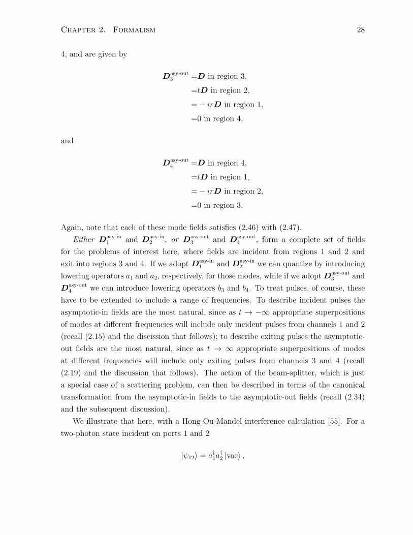
Either Dasy-in1 and Dasy-in
2 , or Dasy-out3 and Dasy-out
4 , form a complete set of fields
for the problems of interest here, where fields are incident from regions 1 and 2 and
exit into regions 3 and 4. If we adopt Dasy-in1 and Dasy-in
2 we can quantize by introducing
lowering operators a1 and a2, respectively, for those modes, while if we adopt Dasy-out3 and
Dasy-out4 we can introduce lowering operators b3 and b4. To treat pulses, of course, these
have to be extended to include a range of frequencies. To describe incident pulses the
asymptotic-in fields are the most natural, since as t → −∞ appropriate superpositions
of modes at different frequencies will include only incident pulses from channels 1 and 2
(recall (2.15) and the discission that follows); to describe exiting pulses the asymptotic-
out fields are the most natural, since as t → ∞ appropriate superpositions of modes
at different frequencies will include only exiting pulses from channels 3 and 4 (recall
(2.19) and the discussion that follows). The action of the beam-splitter, which is just
a special case of a scattering problem, can then be described in terms of the canonical
transformation from the asymptotic-in fields to the asymptotic-out fields (recall (2.34)
and the subsequent discussion).
We illustrate that here, with a Hong-Ou-Mandel interference calculation [55]. For a
two-photon state incident on ports 1 and 2
|ψ12⟩ = a†1a†2 |vac⟩ ,
Chapter 2. Formalism 29
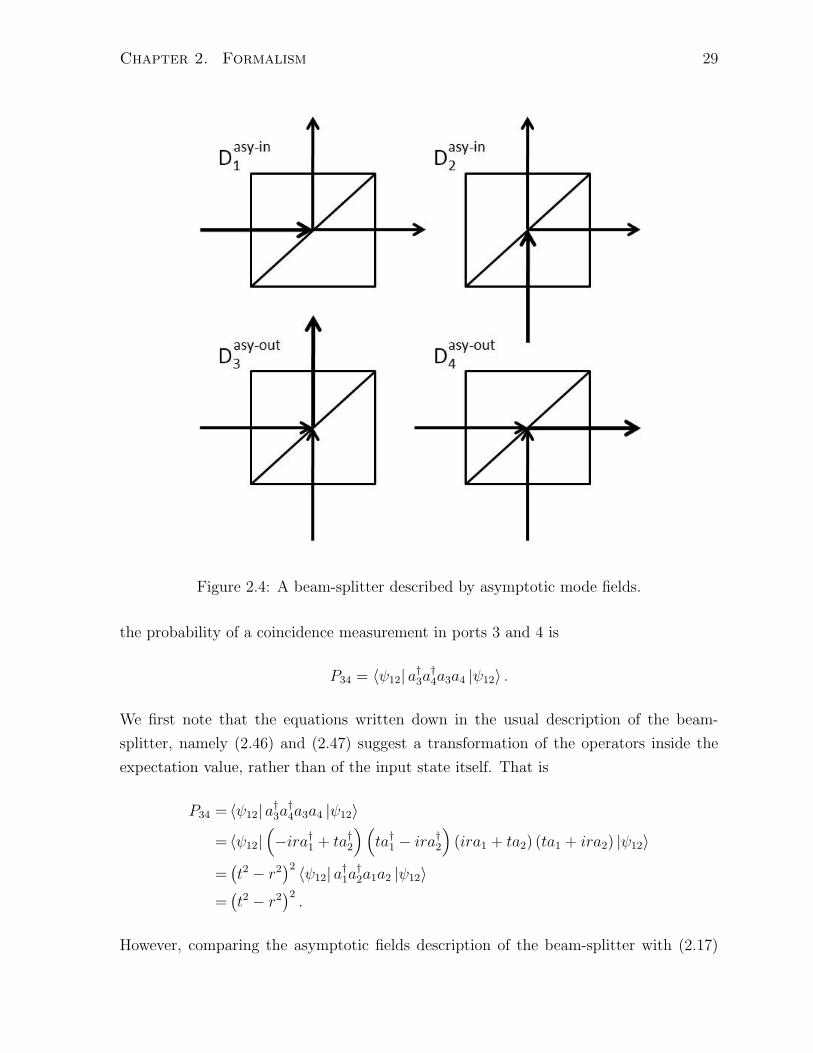
Figure 2.4: A beam-splitter described by asymptotic mode fields.
the probability of a coincidence measurement in ports 3 and 4 is
P34 = ⟨ψ12| a†3a†4a3a4 |ψ12⟩ .
We first note that the equations written down in the usual description of the beam-
splitter, namely (2.46) and (2.47) suggest a transformation of the operators inside the
expectation value, rather than of the input state itself. That is
P34 = ⟨ψ12| a†3a†4a3a4 |ψ12⟩
= ⟨ψ12|(−ira†1 + ta†2
)(ta†1 − ira†2
)(ira1 + ta2) (ta1 + ira2) |ψ12⟩
=(t2 − r2
)2 ⟨ψ12| a†1a†2a1a2 |ψ12⟩
=(t2 − r2
)2.
However, comparing the asymptotic fields description of the beam-splitter with (2.17)
Chapter 2. Formalism 30
shows that for this beam-splitter (2.47) we have, still in our simplified notation
T in3;1 =T in
4;2 = ir
T in4;1 =T in
3;2 = t.
This suggests a transformation of the state as prescribed by (2.35). That is,
|ψ12⟩ =a†1a†2 |vac⟩
=(−irb†3 + tb†4
)(tb†3 − irb†4
)|vac⟩
=[−irt
(b†3b
†3 + b†4b
†4
)+(t2 − r2
)b†3b
†4
]|vac⟩ ,
where we have used (2.37) and so the probability of a coincidence measurement is
P34 = ⟨ψ12| b†3b†4b3b4 |ψ12⟩
=(t2 − r2
) (t2 − r2
)=(t2 − r2
)2,
as expected. Thus it is seen that in linear problems the scattering is described by noth-
ing more than a change of basis from asymptotic-in to asymptotic-out mode fields; the
physics of the scattering is contained within the asymptotic mode fields themselves. If
nonlinearities are included the situation is more complicated, but the strategy devised
here can be extended to aid in the solution of such problems. We turn to that in the
next Section.
2.3 Scattering With Nonlinearities
We now include a nonlinear term in our Hamiltonian,
H = HL +HNL,
assuming that only field operators in the interaction region contribute to HNL. When
HNL is considered explicitly in subsequent Chapters, we will neglect terms (arising from
commutators) that constitute corrections to HL or the ground state expectation value,
as well as terms containing only creation or only annihilation operators, as they do not
approximately conserve energy, a concept that will be more clearly defined at the end
of this Section. This leaves us with a normal-ordered nonlinear Hamiltonian, containing
Chapter 2. Formalism 31
three operators for a second-order nonlinearity or four for a third-order nonlinearity, for
which one can clearly see the destruction of photons leading to the creation of other
photons.
As there is no nonlinearity in the region of excitation, we can still start with a state
|ψ(t0)⟩ at t0 ≪ 0 consisting of energy incident on the interaction region but far from it,
|ψ (t0)⟩ = e−iHLt0/~Kin
(ζnIk(t0)a
†nIk
, ζ∗nIk(t0)anIk
)|vac⟩ ,
where we have introduced the set of variables ζnIk(t) in place of µnIk(t) as now
that we are considering nonlinearities the temporal evolution of the operators may be
more complicated than simple phase accumulation for which ζnIk(t) is just ζnIke−iωnIk(t−t0)
where the ζnIk are complex numbers with units of the square root of length. The temporal
evolution of the ζnIk(t) will be specified below. We define an asymptotic-in ket |ψin⟩as the ket to which this would evolve at t = 0 were there no nonlinearity:
|ψin⟩ = e−iHL(0−t0)/~ |ψ (t0))⟩
= Kin
(ζnIk(t0)a
†nIk
, ζ∗nIk(t0)anIk
)|vac⟩ . (2.49)
In fact the ket evolves according to the entire Hamiltonian H, and at a later time t1 the
ket will be
|ψ (t1)⟩ = e−iH(t1−t0)/~ |ψ (t0)⟩ .
The asymptotic-out ket is the ket that would evolve to this from t = 0 were there no
nonlinearity,
|ψ (t1)⟩ = e−iHL(t1−0)/~ |ψout⟩ , (2.50)
or
|ψout⟩ = eiHLt1/~ |ψ (t1)⟩
= eiHLt1/~e−iH(t1−t0)/~ |ψ (t0)⟩
= eiHLt1/~e−iH(t1−t0)/~e−iHLt0/~ |ψin⟩
= U (t1, t0) |ψin⟩ ,
where
U (t1, t0) ≡ eiHLt1/~e−iH(t1−t0)/~e−iHLt0/~. (2.51)
The entire effect of the nonlinearity is described in the transition |ψin⟩ → |ψout⟩; the rest
of the dynamics in the evolution from |ψ(t0)⟩ → |ψ(t1)⟩ is purely linear and more easily
Chapter 2. Formalism 32
described. In the absence of nonlinearity, of course, H = HL and clearly |ψout⟩ = |ψin⟩.More generally, although the form (2.49) is the easiest in which to specify the incoming
fields, for the ultimate calculation of the out-going fields it is usually more convenient to
use the alternate form
|ψin⟩ = Kout
(ηnIk(t0)b
†nIk
, η∗nIk(t0)bnIk
)|vac⟩ ,
where the variables ηnIk(t) are introduced in place of νnIk (t) for the same reason
ζnIk(t) were introduced in place of µnIk(t), and can be found for a particular state
in terms of ζnIk(t) using (2.35). Then the transition to |ψout⟩ ,
|ψout⟩ = U(t1, t0)Kout
(ηnIk(t0)b
†nIk
, η∗nIk(t0)bnIk
)|vac⟩
can be calculated or approximated using the asymptotic-out basis, as well as, if desired,
the transformation (2.50) to |ψ(t1)⟩. However, we will see that this general strategy can
be simplified in examples we give later.
As an aid in calculating |ψout⟩ we introduce a formal ket |Ψ (t)⟩ according to
|Ψ (t)⟩ = U (t, t0) |ψin⟩ , (2.52)
where t varies from t0 to t1, and so
|ψin⟩ = |Ψ (t0)⟩ ,
|ψout⟩ = |Ψ (t1)⟩ . (2.53)
From its definition (2.51) we have
i~dU (t, t0)
dt= eiHLt/~ (−HL +H) e−iH(t−t0)/~e−iHLt0/~
= eiHLt/~HNLe−iH(t−t0)/~e−iHLt0/~
= eiHLt/~HNLe−iHLt/~eiHLt/~e−iH(t−t0)/~e−iHLt0/~
= eiHLt/~HNLe−iHLt/~U (t, t0)
= V(b†nIk
, bnIk ; t
)U (t, t0) ,
where we have defined
V(b†nIk
, bnIk ; t
)= eiHLt/~HNLe
−iHLt/~, (2.54)
Chapter 2. Formalism 33
and so in particular
i~d
dt|Ψ (t)⟩ = V
(b†nIk
, bnIk ; t
)|Ψ (t)⟩ . (2.55)
At times t1 > t > t0 we then seek a |Ψ (t)⟩ of the form
|Ψ (t)⟩ = Kout
(ηnIk (t) b†nIk
, η∗nIk (t) bnIk
) ∣∣∣Ψ (t)⟩, (2.56)
such that the evolution of∣∣∣Ψ (t)
⟩then follows from the dynamics of |Ψ (t)⟩. From (2.53)
and (2.49) it is clear that ∣∣∣Ψ (t0)⟩
= |vac⟩ ,
and from (2.52), (2.49), and (2.56) we have
|ψin⟩ = |Ψ (t0)⟩ = Kout
(ηnIk (t0) b
†nIk
, η∗nIk (t0) bnIk
) ∣∣∣Ψ (t0)⟩,
|ψout⟩ = |Ψ (t1)⟩ = Kout
(ηnIk (t1) b
†nIk
, η∗nIk (t1) bnIk
) ∣∣∣Ψ (t1)⟩, (2.57)
so the problem of finding |ψout⟩ from |ψin⟩ is reduced to the problem of evolving∣∣∣Ψ (t)
⟩from t0 to t1. This task can be simplified by choosing a proper evolution of the ηnIk (t).
At least roughly speaking, it is clear that the “best” η (t) – in the sense that the
evolution of the resulting∣∣∣Ψ (t)
⟩from t0 to t1 is best approximated as the state just
remaining in the vacuum – identifies the “best” evolution of the asymptotic-in ket in the
absence of photon generation.
From (2.56) we have∣∣∣Ψ(t)⟩
= K†out
(ηnIk (t) b†nIk
, η∗nIk (t) bnIk
)|Ψ (t)⟩ ,
Chapter 2. Formalism 34
so
i~d
dt
∣∣∣Ψ(t)⟩
=
(i~
d
dtK†
out
(ηnIk (t) b†nIk
, η∗nIk (t) bnIk
))|Ψ (t)⟩
+K†out
(ηnIk (t) b†nIk
, η∗nIk (t) bnIk
)V(b†nIk
, bnIk ; t
)|Ψ (t)⟩
=
(i~
d
dtK†
out
(ηnIk (t) b†nIk
, η∗nIk (t) bnIk
))×Kout
(ηnIk (t) b†nIk
, η∗nIk (t) bnIk
) ∣∣∣Ψ (t)⟩
+K†out
(ηnIk (t) b†nIk
, η∗nIk (t) bnIk
)V(b†nIk
, bnIk ; t
)×Kout
(ηnIk (t) b†nIk
, η∗nIk (t) bnIk
) ∣∣∣Ψ (t)⟩, (2.58)
where we have used (2.55). Defining
Hb (t)K†out
(ηnIk (t) b†nIk
, η∗nIk (t) bnIk
)≡ i~
d
dtK†
out
(ηnIk (t) b†nIk
, η∗nIk (t) bnIk
),
(2.59)
and
V (t) ≡K†out
(ηnIk (t) b†nIk
, η∗nIk (t) bnIk
)V(b†nIk
, anIk ; t
)×Kout
(ηnIk (t) b†nIk
, η∗nIk (t) bnIk
), (2.60)
we rewrite (2.58) as
i~d
dt
∣∣∣Ψ (t)⟩
= H (t)∣∣∣Ψ (t)
⟩,
where
H (t) = Hb (t) + V (t) .
For the particular case of a generalized coherent state as the asymptotic-in state
|ψin⟩ = exp
( ∑n,I∈σn
∫ ∞
0
dk ζnIk (t0) a†nIk − H.c.
)∣∣∣Ψ (t0)⟩
= exp
( ∑n,I∈σn
∫ ∞
0
dk ηnIk(t0)b†nIk − H.c.
)∣∣∣Ψ (t0)⟩,
where
ηnIk(t0) =∑
n′,I′∈σn′
∫ ∞
0
dk′T outn′I′;nI (k′, k) ζn′I′k′ (t0) ,
Chapter 2. Formalism 35
we have, using a Baker-Campbell-Hausdorff relation [47],
K†out
(ηnIk (t) b†nIk
, η∗nIk (t) bnIk
)= exp
(−∑
n,I∈σn
∫ ∞
0
dk ηnIk(t)b†nIk +∑
n,I∈σn
∫ ∞
0
dk η∗nIk(t)bnIk
)
= exp
(−∑
n,I∈σn
∫ ∞
0
dk ηnIk(t)b†nIk
)exp
( ∑n,I∈σn
∫ ∞
0
dk η∗nIk(t)bnIk
)
× exp
(−1
2
∑n,I∈σn
∫ ∞
0
dk |ηnIk(t)|2).
Furthermore, using
exp
(−∑
n,I∈σn
∫ ∞
0
dk ηnIk(t0)b†nIk + H.c.
)bnIk exp
( ∑n,I∈σn
∫ ∞
0
dk ηnIk(t0)b†nIk − H.c.
)=bnIk + ηnIk (t) ,
we find (recall (2.59))
Hb (t) =i~2
∑n,I∈σn
∫ ∞
0
dk
[(dη∗nIk(t)
dtηnIk(t) − η∗nIk(t)
dηnIk(t)
dt
)+ 2
(dη∗nIk(t)
dtbnIk −
dηnIk(t)
dtb†nIk
)],
as well as
V (t) = V(b†nIk + η∗nIk (t)
, bnIk + ηnIk (t) ; t
),
and recognize that by a proper choice of the dynamics of ηnIk(t) we can eliminate terms
in V (t) that are first order in the operators. The equations the ηnIk(t) satisfy are the
equations that would follow for the asymptotic-out mode amplitudes in the corresponding
classical problem; they include the full classical nonlinear evolution through the material,
including the classical generation of any higher harmonics, the classical mixing of any
combinations of frequencies, and the like. Of course, they need not be determined by
solving those equations; they can be determined with the aid of whatever approximations
might be appropriate, or even from a numerical solution of the nonlinear equations for the
Maxwell fields, and then extracting the ηnIk(t). But however they are determined, their
use in (2.56) describes how the quantum problem would evolve if the modes remained in
coherent states with amplitudes determined by these classical solutions. All “quantum
Chapter 2. Formalism 36
effects” are contained in how the “new” H(t) will cause∣∣∣Ψ(t)
⟩to differ from the vacuum
as t varies from t0 to t1. As such, the operatorsb†nIk
and bnIk now appearing in
H(t) can be understood as operators that describe fluctuations about the classical state
described by the ηnIk. Particular examples will be presented in the next Chapter.
With terms that are first order in the operators eliminated, it is clear that we may
split H(t) into a piece that involves a single raising operator followed by a single lowering
operator, which we call HX (t), as well as a piece consisting of terms that involve no
operators (and thus have no influence on the dynamics of the fields), or two raising or
two lowering operators, or higher powers of operators, which we call Hrest (t). Loosely
speaking, the first piece corresponds to self- and cross-modulation-like terms while the
second to photon pair generation and squeezing-like terms. The goal is thus to solve
i~d
dt
∣∣∣Ψ(t)⟩
= (HX (t) +Hrest (t))∣∣∣Ψ(t)
⟩, (2.61)
subject to the initial condition ∣∣∣Ψ(t0)⟩
= |vac⟩ , (2.62)
so that we may determine
|ψout⟩ = exp
( ∑n,I∈σn
∫ ∞
0
dk ηnIk(t1)b†nIk − H.c.
)∣∣∣Ψ(t1)⟩.
The coherent state in front of∣∣∣Ψ(t1)
⟩is what |ψin⟩ would evolve to were there no non-
linearity. To solve (2.61) we introduce an evolution operator of the form
U (t, t′) = UX (t, t′)Urest (t, t′) ,
such that ∣∣∣Ψ(t)⟩
= U (t, t′)∣∣∣Ψ(t′)
⟩,
with
i~dUX (t, t′)
dt= HX (t)UX (t, t′) , (2.63)
and
UX (t, t′) |vac⟩ = U †X (t, t′) |vac⟩ = |vac⟩ . (2.64)
Chapter 2. Formalism 37
From (2.61) it is seen that the evolution operator satisfies
i~dU (t, t′)
dt= (HX (t) +Hrest (t))U (t, t′) ,
and thus
i~dUrest (t, t′)
dt= U †
X (t, t′)Hrest (t)UX (t, t′)Urest (t, t′) . (2.65)
Finally, applying Theorem III from the classic paper of Magnus [56], namely that
d
dtU (t) = A (t)U (t) ,
has solution
U (t) = eΩ(t),
where
Ω (t) =
∫ t
0
A (τ) dτ +1
2
∫ t
0
[A (τ) ,
∫ τ
0
A (σ) dσ
]dτ + · · · , (2.66)
we find the solution for (2.65) to first order in the nonlinearity
dUrest (t, t′)
dt= exp
(1
i~
∫ t
t′U †X (τ, t′)Hrest (τ)UX (τ, t′) dτ
),
and are able to solve∣∣∣Ψ(t1)⟩
= U (t1, t0)∣∣∣Ψ(t0)
⟩= UX (t1, t0)Urest (t1, t0)U
†X (t1, t0) |vac⟩
= U †X (t0, t1) exp
(1
i~
∫ t1
t0
U †X (τ, t0)Hrest (τ)UX (τ, t0) dτ
)UX (t0, t1) |vac⟩
= exp
(1
i~
∫ t1
t0
U †X (τ, t1)Hrest (τ)UX (τ, t1) dτ
)|vac⟩ , (2.67)
where we have used (2.62) and (2.64) in the second line, as well as (A.10) in the third
and (A.9) in the fourth. We note that the time integral in (2.67), via the exponential
factors introduced through (2.54), determines which terms in Hrest (τ) are approximately
energy conserving. The longer the time from t0 to t1 the stronger the requirement that
the exponential factors approximately sum to zero. Terms with exponential factors that
do not approximately sum to zero may be neglected with little error. Returning to the
discussion at the start of this Section, it is clearly not possible for the exponential factors
to sum to zero if all of the factors have the same sign, i.e. if they all result from creation
Chapter 2. Formalism 38
operators or all result from annihilation operators.
Lastly, if we consider a general operator, O, residing in Hrest (τ) and ask how it evolves
under the unitary transformation U †X (t, t′)OUX (t, t′) ≡ O (t) seen in (2.67), we can use
(2.63) to show
i~d
dtO (t) =
[O (t) , HX (t)
],
subject to the initial condition
O (t′) = U †X (t′, t′)OUX (t′, t′)
= O.
This completes the specification of∣∣∣Ψ(t1)
⟩and thus |ψout⟩.
2.4 Discussion
In this Chapter I have presented a Hamiltonian formalism useful for calculations in
nonlinear classical and quantum optics which is applicable to a large variety of photonic
systems, from integrated circuits to layered structures. It exploits asymptotic-in and
asymptotic-out fields, in close analogy with scattering theory in quantum mechanics.
These fields are the stationary solutions of the classical linear Maxwell equations, and
can be evaluated analytically or numerically. In Section 2.1 it was demonstrated that
such solutions can be used to describe the electromagnetic field in either a classical or
a quantum framework, and so from the results of classical calculations it is possible
to construct an appropriate Hamiltonian associated with the problem of interest. In
particular, in Section 2.2 it was shown that the linear scattering problem can be viewed
as a basis transformation from that of asymptotic-in fields to that of asymptotic-out
fields. In Section 2.3 this strategy was applied to the description of scattering in the
presence of nonlinearities.
Examples in Chapter 3 illustrate the versatility of this approach. They show how
this strategy leverages solutions of the classical linear Maxwell equations, found either
analytically or numerically, to simplify the solution of nonlinear classical or quantum
problems. They also show how it highlights the physics of the nonlinear interaction and
its enhancement in cavity structures.
Chapter 3
Power Scaling Relationships
With the formalism established in the previous Chapter, I now employ it to calculate the
average number of photons generated in integrated devices under various pumping situa-
tions. The formalism places quantum and corresponding classical wave mixing processes
in both straight waveguides and cavity structures on equal theoretical footing, making
it easy to compare how one process scales relative to another while identifying common
terms.
Note that there is a difference between what is meant by corresponding processes, and
reverse processes. For the purposes of this Chapter, corresponding processes are pumped
at the same frequency whereas reverse processes have opposite pump and generated
frequencies (see Fig. 3.1). For example, SPDC is a quantum χ2 process in which a pump
photon at ωP is converted into a photon at each ωS and ωI, with ωP = ωS + ωI (see Fig.
3.2). The classical χ2 process corresponding to SPDC is DFG, in which a pump photon at
ωP as well as a seed photon at ωS create a photon at ωI. SPDC’s reverse process, on the
other hand, is sum frequency generation (SFG) in which pump photons at each ωS and
ωI are converted into a photon at ωP. Similarly the classical χ3 process corresponding to
SFWM, where two pump photons at ωP are converted into a photon at each ωS and ωI,
with 2ωP = ωS + ωI (see Fig. 3.2), is FWM, where two pump photons at ωP as well as a
seed photon at ωS lead to a photon at ωI. The χ3 process that is the reverse of SFWM is
dual-pump SFWM, in which photons at each ωS and ωI are converted into two photons
at ωP. While it is true that knowledge of the efficiency of the classical reverse process of a
quantum process in a given device - or indeed that of any nonlinear optical process of the
same order as the quantum process - will allow one to infer something about the efficiency
of said quantum process in the same device, it is convenient to compare quantum and
classical processes each pumped at the same frequency. Therefore this Chapter focuses
on corresponding processes.
39
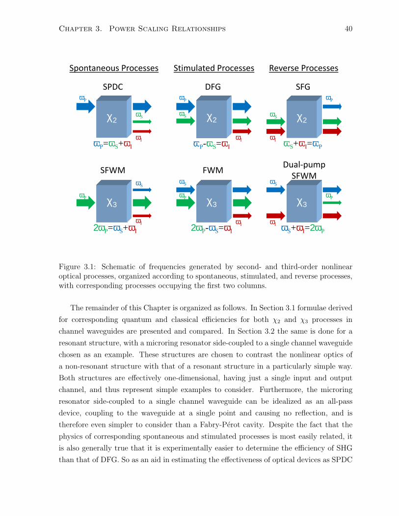
Chapter 3. Power Scaling Relationships 40
Stimulated ProcessesSpontaneous Processes Reverse Processes
ωP
χ2
ωI
DFG
ωP-ωS=ωI
SFG
χ2ωS
ωS+ωI=ωP
ωP
ωIωP=ωS+ωI
ωP
χ2ωS
SPDC
ωI
ωS
χ3
FWM
ωP-ωS=ωI
ωP
ωS
2ωP-ωS=ωI
ωI
χ3
Dual-pump
SFWM
ωS+ωI=ωP
ωS
ωS+ωI=2ωP
ωP
ωI
SFWM
ωP=ωS+ωI
χ3
2ωP=ωS+ωI
ωP
ωS
ωI
Figure 3.1: Schematic of frequencies generated by second- and third-order nonlinearoptical processes, organized according to spontaneous, stimulated, and reverse processes,with corresponding processes occupying the first two columns.
The remainder of this Chapter is organized as follows. In Section 3.1 formulae derived
for corresponding quantum and classical efficiencies for both χ2 and χ3 processes in
channel waveguides are presented and compared. In Section 3.2 the same is done for a
resonant structure, with a microring resonator side-coupled to a single channel waveguide
chosen as an example. These structures are chosen to contrast the nonlinear optics of
a non-resonant structure with that of a resonant structure in a particularly simple way.
Both structures are effectively one-dimensional, having just a single input and output
channel, and thus represent simple examples to consider. Furthermore, the microring
resonator side-coupled to a single channel waveguide can be idealized as an all-pass
device, coupling to the waveguide at a single point and causing no reflection, and is
therefore even simpler to consider than a Fabry-Perot cavity. Despite the fact that the
physics of corresponding spontaneous and stimulated processes is most easily related, it
is also generally true that it is experimentally easier to determine the efficiency of SHG
than that of DFG. So as an aid in estimating the effectiveness of optical devices as SPDC
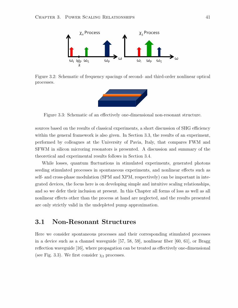
Chapter 3. Power Scaling Relationships 41
Figure 3.2: Schematic of frequency spacings of second- and third-order nonlinear opticalprocesses.
Figure 3.3: Schematic of an effectively one-dimensional non-resonant structure.
sources based on the results of classical experiments, a short discussion of SHG efficiency
within the general framework is also given. In Section 3.3, the results of an experiment,
performed by colleagues at the University of Pavia, Italy, that compares FWM and
SFWM in silicon microring resonators is presented. A discussion and summary of the
theoretical and experimental results follows in Section 3.4.
While losses, quantum fluctuations in stimulated experiments, generated photons
seeding stimulated processes in spontaneous experiments, and nonlinear effects such as
self- and cross-phase modulation (SPM and XPM, respectively) can be important in inte-
grated devices, the focus here is on developing simple and intuitive scaling relationships,
and so we defer their inclusion at present. In this Chapter all forms of loss as well as all
nonlinear effects other than the process at hand are neglected, and the results presented
are only strictly valid in the undepleted pump approximation.
3.1 Non-Resonant Structures
Here we consider spontaneous processes and their corresponding stimulated processes
in a device such as a channel waveguide [57, 58, 59], nonlinear fiber [60, 61], or Bragg
reflection waveguide [16], where propagation can be treated as effectively one-dimensional
(see Fig. 3.3). We first consider χ2 processes.
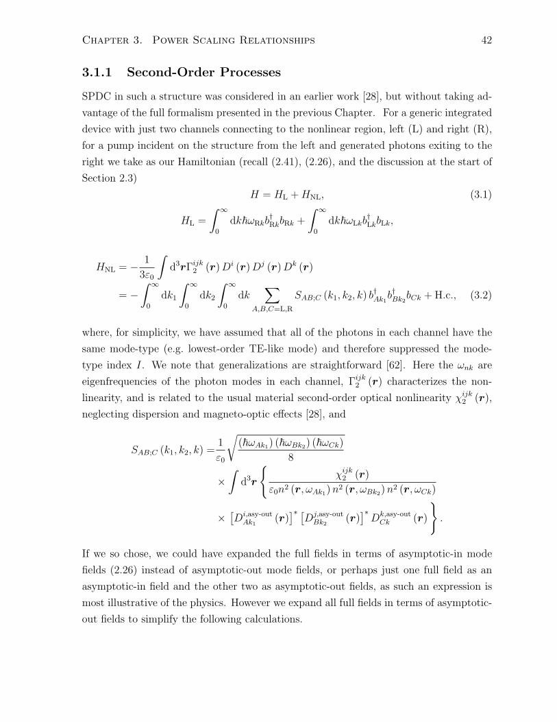
Chapter 3. Power Scaling Relationships 42
3.1.1 Second-Order Processes
SPDC in such a structure was considered in an earlier work [28], but without taking ad-
vantage of the full formalism presented in the previous Chapter. For a generic integrated
device with just two channels connecting to the nonlinear region, left (L) and right (R),
for a pump incident on the structure from the left and generated photons exiting to the
right we take as our Hamiltonian (recall (2.41), (2.26), and the discussion at the start of
Section 2.3)
H = HL +HNL, (3.1)
HL =
∫ ∞
0
dk~ωRkb†RkbRk +
∫ ∞
0
dk~ωLkb†LkbLk,
HNL = − 1
3ε0
∫d3rΓijk
2 (r)Di (r)Dj (r)Dk (r)
= −∫ ∞
0
dk1
∫ ∞
0
dk2
∫ ∞
0
dk∑
A,B,C=L,R
SAB;C (k1, k2, k) b†Ak1b†Bk2
bCk + H.c., (3.2)
where, for simplicity, we have assumed that all of the photons in each channel have the
same mode-type (e.g. lowest-order TE-like mode) and therefore suppressed the mode-
type index I. We note that generalizations are straightforward [62]. Here the ωnk are
eigenfrequencies of the photon modes in each channel, Γijk2 (r) characterizes the non-
linearity, and is related to the usual material second-order optical nonlinearity χijk2 (r),
neglecting dispersion and magneto-optic effects [28], and
SAB;C (k1, k2, k) =1
ε0
√(~ωAk1) (~ωBk2) (~ωCk)
8
×∫
d3r
χijk2 (r)
ε0n2 (r, ωAk1)n2 (r, ωBk2)n
2 (r, ωCk)
×[Di,asy-out
Ak1(r)]∗ [
Dj,asy-outBk2
(r)]∗Dk,asy-out
Ck (r)
.
If we so chose, we could have expanded the full fields in terms of asymptotic-in mode
fields (2.26) instead of asymptotic-out mode fields, or perhaps just one full field as an
asymptotic-in field and the other two as asymptotic-out fields, as such an expression is
most illustrative of the physics. However we expand all full fields in terms of asymptotic-
out fields to simplify the following calculations.

Chapter 3. Power Scaling Relationships 43
Note that we can also write an asymptotic-in ket of the form
|ψin⟩ = exp
(∫ ∞
0
dkζLk (t0) a†Lk − H.c.
)|vac⟩ ,
in terms of b†nk operators instead of a†nk operators, that is
|ψin⟩ = exp
( ∑C=L,R
∫ ∞
0
dkηCk (t0) b†Ck − H.c.
)|vac⟩ ,
where
ηCk (t0) =
∫ ∞
0
dk′T outL;C(k′, k)ζLk′ (t0) .
However, restricting ourselves to devices that are all-pass filters (i.e. devices that do not
reflect the pump pulse back along the same channel) we can simplify this as
|ψin⟩ = exp
(∫ ∞
0
dkηRk (t0) b†Rk − H.c.
)|vac⟩ ,
where
ηRk (t0) =
∫ ∞
0
dk′T outL;R(k′, k)ζLk′ (t0) ,
and find (recall (2.59), (2.54), and (2.60))
Hb (t) =i~2
∫ ∞
0
dk
[(dη∗Rk (t)
dtηRk (t) − η∗Rk (t)
dηRk (t)
dt
)+ 2
(dη∗Rk (t)
dtbRk −
dηRk (t)
dtb†Rk
)],
V (t) = −∫ ∞
0
dk1
∫ ∞
0
dk2
∫ ∞
0
dk∑
A,B,C=L,R
[SAB;C (k1, k2, k; t)
(b†Ak1
+ η∗Rk1(t) δAR
)×(b†Bk2
+ η∗Rk2(t) δBR
)(bCk + ηRk (t) δCR
)+ H.c.
], (3.3)
where
SAB;C (k1, k2, k; t) = SAB;C (k1, k2, k) ei(ωAk1+ωBk2
−ωCk)t. (3.4)
This expression identifies approximately energy conserving terms as those for which
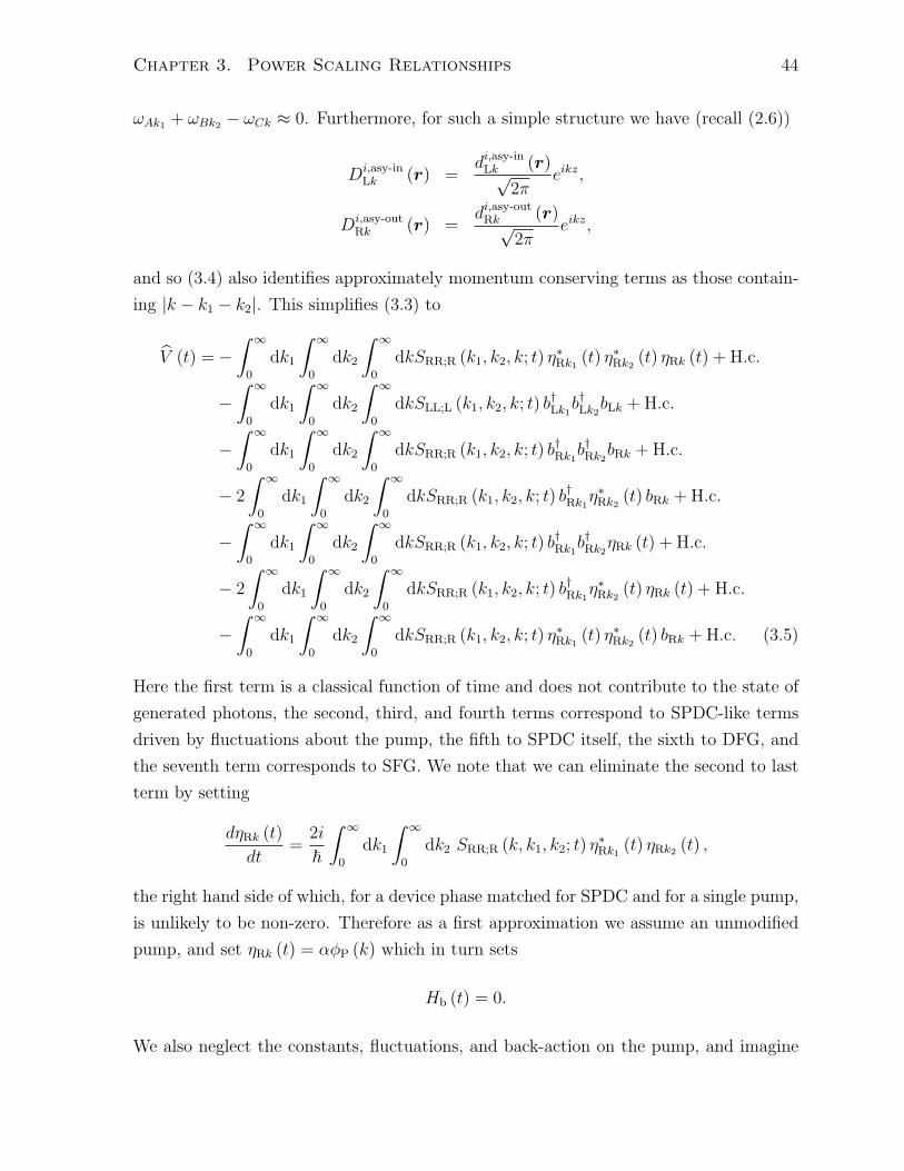
Chapter 3. Power Scaling Relationships 44
ωAk1 + ωBk2 − ωCk ≈ 0. Furthermore, for such a simple structure we have (recall (2.6))
Di,asy-inLk (r) =
di,asy-inLk (r)√2π
eikz,
Di,asy-outRk (r) =
di,asy-outRk (r)√2π
eikz,
and so (3.4) also identifies approximately momentum conserving terms as those contain-
ing |k − k1 − k2|. This simplifies (3.3) to
V (t) = −∫ ∞
0
dk1
∫ ∞
0
dk2
∫ ∞
0
dkSRR;R (k1, k2, k; t) η∗Rk1(t) η∗Rk2
(t) ηRk (t) + H.c.
−∫ ∞
0
dk1
∫ ∞
0
dk2
∫ ∞
0
dkSLL;L (k1, k2, k; t) b†Lk1b†Lk2bLk + H.c.
−∫ ∞
0
dk1
∫ ∞
0
dk2
∫ ∞
0
dkSRR;R (k1, k2, k; t) b†Rk1b†Rk2
bRk + H.c.
− 2
∫ ∞
0
dk1
∫ ∞
0
dk2
∫ ∞
0
dkSRR;R (k1, k2, k; t) b†Rk1η∗Rk2
(t) bRk + H.c.
−∫ ∞
0
dk1
∫ ∞
0
dk2
∫ ∞
0
dkSRR;R (k1, k2, k; t) b†Rk1b†Rk2
ηRk (t) + H.c.
− 2
∫ ∞
0
dk1
∫ ∞
0
dk2
∫ ∞
0
dkSRR;R (k1, k2, k; t) b†Rk1η∗Rk2
(t) ηRk (t) + H.c.
−∫ ∞
0
dk1
∫ ∞
0
dk2
∫ ∞
0
dkSRR;R (k1, k2, k; t) η∗Rk1(t) η∗Rk2
(t) bRk + H.c. (3.5)
Here the first term is a classical function of time and does not contribute to the state of
generated photons, the second, third, and fourth terms correspond to SPDC-like terms
driven by fluctuations about the pump, the fifth to SPDC itself, the sixth to DFG, and
the seventh term corresponds to SFG. We note that we can eliminate the second to last
term by setting
dηRk (t)
dt=
2i
~
∫ ∞
0
dk1
∫ ∞
0
dk2 SRR;R (k, k1, k2; t) η∗Rk1
(t) ηRk2 (t) ,
the right hand side of which, for a device phase matched for SPDC and for a single pump,
is unlikely to be non-zero. Therefore as a first approximation we assume an unmodified
pump, and set ηRk (t) = αϕP (k) which in turn sets
Hb (t) = 0.
We also neglect the constants, fluctuations, and back-action on the pump, and imagine
Chapter 3. Power Scaling Relationships 45
the pump to contain photons at roughly twice the frequency of the generated photons,
leading us to keep only
Hb (t) + V (t) = −α∫ ∞
0
dk1
∫ ∞
0
dk2
∫ ∞
0
dkSRR;R (k1, k2, k; t) b†Rk1b†Rk2
ϕP (k) + H.c.
This greatly simplifies the calculation of the output state, as here UX (t1, t0) = I, (recall
(2.63)) and we find (recall (2.57) and (2.67))
|ψout⟩ = exp
(α
∫ ∞
0
dkϕP (k) b†Rk − H.c.
)|ψgen⟩ ,
where
|ψgen⟩ = exp
(iα
~
∫ ∞
0
dk1
∫ ∞
0
dk2
∫ ∞
0
dkϕP (k)
×[∫ t1
t0
dτSRR;R (k1, k2, k; τ)
]b†Rk1
b†Rk2− H.c.
)|vac⟩ .
With the nonlinearity centered at r = 0 such that the pump pulse only interacts with it
for times near t = 0, we extend t0 → −∞, and t1 → ∞, and find that the state of SPDC
generated photons in a two-channel device due to an exciting pump pulse can be written
as the single-mode squeezed vacuum
|ψgen⟩ = exp
(β√2
∫ ∞
0
dk1
∫ ∞
0
dk2ϕ (k1, k2) b†Rk1
b†Rk2− H.c.
)|vac⟩ ,
where |β|2 is proportional to the average number of photons in the pump pulse NP = |α|2
and
ϕ (k1, k2) =2√
2πα
β
i
~
∫ ∞
0
dkϕP (k)SRR;R (k1, k2, k) δ (ωRk1 + ωRk2 − ωRk) . (3.6)
Alternately, switching to a description in terms of frequency rather than wavenumber
[28],
|ψgen⟩ = exp(βC†
II − H.c.)|vac⟩ , (3.7)
where
C†II =
1√2
∫ ∞
0
dω1
∫ ∞
0
dω2ϕ (ω1, ω2) b†Rω1
b†Rω2, (3.8)
Chapter 3. Power Scaling Relationships 46
such that C†II |vac⟩ is a normalized two-photon state characterized by the BWF
ϕ (ω1, ω2) =iπ
√dk (ω1)
dω1
√dk (ω2)
dω2
(√dk (ω)
dω
)ω=ω1+ω2
×
√~ (ω1 + ω2)ω1ω2 (χ2)
2 NP
ε0 |β|2 n6ϕP (ω1 + ω2) J (ω1, ω2) , (3.9)
with
J (ω1, ω2) =n3
χ2
∫d3r
χijk (r)
ε3/20 n2 (r, ω1)n2 (r, ω2)n2 (r, ω1 + ω2)
×[Di,asy-out
Rk(ω1)(r)]∗ [
Dj,asy-outRk(ω2)
(r)]∗Dk,asy-out
Rk(ω1+ω2)(r)
, (3.10)
and the n and χ2 are, respectively, a typical value of refractive index and a typical
value of second-order nonlinearity introduced solely for convenience. We note that the
BWF contains information about the correlations between generated photons that can
be expressed in terms of frequency (3.9), wavenumber
ϕ (k1, k2) =
√dk (ω1)
dω1
√dk (ω2)
dω2
−1
ϕ (ω1, ω2) ,
or even time
ϕ (t1, t2) =1
2π
∫dω1dω2ϕ (ω1, ω2) e
i(ω1t1+ω2t2).
However, as we view said correlations to be the result of energy (and momentum) conser-
vation, in this thesis we prefer to work with BWFs represented in the frequency domain.
While everything above has been quite general, for the kind of device considered here,
a channel waveguide in which all propagation, from channel L through the nonlinearity
to channel R, occurs along the z direction
Di,asy-inLk(ω) (r) = Di,asy-out
Rk(ω) (r) = dik(ω) (x, y)eikz√
2π, (3.11)
and so we drop the redundant label R for the remainder of this Section. This simplifies
Chapter 3. Power Scaling Relationships 47
(3.9) to
ϕ (ω1, ω2) =iL
√dk (ω1)
dω1
√dk (ω2)
dω2
(√dk (ω)
dω
)ω=ω1+ω2
×
√ω1ω2 (χ2)
2 NP
8πε0 |β|2 n6
√~ (ω1 + ω2)
A [k (ω1) , k (ω2) , k (ω1 + ω2)]
× ϕP (ω1 + ω2) sinc [k (ω1) + k (ω2) − k (ω1 + ω2)]L/2 , (3.12)
where L is the length of the nonlinear structure, and
A [k (ω1) , k (ω2) , k (ω1 + ω2)]
=
∣∣∣∣∣∣∫
dxdyn3χijk
2 (x, y)[dik(ω1)
(x, y)]∗ [
djk(ω2)(x, y)
]∗dkk(ω1+ω2)
(x, y)
χ2ε3/20 n2 (x, y;ω1)n2 (x, y;ω2)n2 (x, y;ω1 + ω2)
∣∣∣∣∣∣−2
, (3.13)
is an effective area with dik(ω) (x, y) the i-th component of the displacement field at fre-
quency ω, and n (x, y;ω) the material refractive index at frequency ω, both at waveguide
cross-sectional position (x, y), and we have chosen the mode amplitudes such that we can
take the phase associated with the effective area to be zero [28].
That C†II |vac⟩ is normalized requires∫ ∞
0
dω1
∫ ∞
0
dω2 |ϕ (ω1, ω2)|2 = 1,
which in turn determines |β|. In the limit |β| ≪ 1,
|ψgen⟩ ≈ |vac⟩ + βC†II |vac⟩ ,
and 2 |β|2 ≡ ND can be thought of as the average number of generated photons per pump
pulse. Indeed this line of thinking holds even in the limit of a pulse long enough that its
intensity spectrum that can be approximated as a Dirac delta function, |ϕP (ω1 + ω2)|2 ≈δ (ω1 + ω2 − ωP), in comparison to the phase matching sinc function of the BWF of
(3.12); the result for ND is then
ND =2~ωPNPL
2
PAT, (3.14)
provided |β| ≪ 1. Note that in deriving (3.14) we have integrated over ω2, and taken the
effective area, A, and group velocities, v−1SH(F ) = (dk/dω)ω=ωP (ωP /2), as constant over the
Chapter 3. Power Scaling Relationships 48
generation bandwidth time
T =2π∫ ωP/2
0dΩ[1 − (2Ω/ωP)2
]sinc2 [k (ωP/2 + Ω) + k (ωP/2 − Ω) − k (ωP)]L/2
,
(3.15)
where Ω = ω1 − ωP/2 represents positive detuning from ωP/2, and P =
8ε0n6v2FvSH/ (χ2ωP)2 is a characteristic power for a χ2 material [2]. Yet it is also true that
if we consider a constant rate of pump photons or average pump power, PP = ~ωPNP/T ,
where T is the time that the pump is on, ND/T = 2PPL2/(PAT ) can be thought of as
the average rate of generated photons provided that |β| √p1 ≪ 1, where√p1 is the largest
Schmidt coefficient in a Schmidt decomposition [63] of the BWF. For if one writes (3.8)
in the basis of the Schmidt modes, and calculates the expectation value of the number of
photons in (3.7), one sees that (3.14) remains true in the continuous wave (CW) limit,
provided PP ≪ PA/L2 (see (B.6)). Defining PI = ~ωFND/ (2T ) as the average generated
power associated with one photon of each pair, we rewrite (3.14) as
PI =~ωF
TPPL
2
PA. (3.16)
To derive expressions for classical second-order nonlinear processes we begin with
the same Hamiltonian as above (3.1) and proceed more or less as above, yet keeping
different terms. For a DFG calculation, we take the pump and signal as both incident
from the left and, while they may or may not exist in two distinct propagation modes
of the waveguide, take their center frequencies separated enough that we can still give
them distinct labels aLSk ≡ aSk, and aLPk ≡ aPk, with[aSk, a
†Pk
]= 0. This is certainly
true for a CW calculation. We take as our input state
|ψin⟩ = exp
(∑I=S,P
∫ ∞
0
dkηIk (t0) b†Ik − H.c.
)|vac⟩ , (3.17)
and, making approximations similar to above find
Hb (t)+V (t) = −2α∗SαP
∫ ∞
0
dk
∫ ∞
0
dk1
∫ ∞
0
dk2SRR;R (k, k1, k2; t) b†Rkϕ
∗S (k1)ϕP (k2)+H.c.,
and thus
|ψgen⟩ = exp
(β
∫ ∞
0
dωϕ (ω) b†Rω − H.c.
)|vac⟩ ,
Chapter 3. Power Scaling Relationships 49
with the single photon wave function
ϕ (ω) =√
2iπ
∫ ∞
0
dω1
√dk (ω)
dω
√dk (ω1)
dω1
√dk (ω2)
dω2
ω2=ω+ω1
×
√~ωω1 (ω + ω1) (χ2)
2 |αS|2 |αP|2
ε0 |β|2 n6ϕ∗S (ω1)ϕP (ω + ω1) J (ω, ω1)
, (3.18)
where
ϕI (ω) =sin [(ω − ωI)T/2]
(ω − ωI)√πT/2
, (3.19)
and J (ω1, ω2) is as above (3.10). Note that here, under the undepleted pump approxi-
mation, |β|2 corresponds to the number of generated idler photons.
For a channel waveguide (3.11)
ϕ (ω) =iL
∫ ∞
0
dω1
√dk (ω)
dω
√dk (ω1)
dω1
√dk (ω2)
dω2
ω2=ω+ω1
×
√ωω1 (χ2)
2 |αS|2 |αP|2
4πε0 |β|2 n6
√~ (ω + ω1)
A [k (ω) , k (ω1) , k (ω + ω1)]
× ϕ∗S (ω1)ϕP (ω + ω1) sinc [k (ω) + k (ω1) − k (ω + ω1)]L/2
.
If we make the approximation∣∣∣∣∫ ∞
0
dω1
√ω1 (ω + ω1)ϕ
∗S (ω)ϕP (ω + ω1) sinc [k (ω) + k (ω1) − k (ω + ω1)]L/2
∣∣∣∣2≈ ωS (ω + ωS) sinc2 [k (ω) + k (ωS) − k (ω + ωS)]L/2
∣∣∣∣∫ ∞
−∞dω1ϕ
∗S (ω1)ϕP (ω + ω1)
∣∣∣∣2= ωS (ω + ωS) sinc2 [k (ω) + k (ωS) − k (ω + ωS)]L/2 2π
T|ϕP (ω + ωS)|2 , (3.20)
then, as the normalization∫∞0
dω |ϕ (ω)|2 = 1 determines |β|, in the CW limit, we can
calculate
|β|2 =~ (ωP − ωS) |αS|2
T
2 |αP|2 L2
PAsinc2 [k (ωP − ωS) + k (ωS) − k (ωP)]L/2 ,
where we have taken ωP = ωSH, vP = vSH, and assumed that the signal frequency is close
Chapter 3. Power Scaling Relationships 50
enough to half the pump frequency that, outside the sinc function, ωS ≈ ωP−ωS ≈ ωP/2
as well as (dk/dω)ω=(ωS)≈ (dk/dω)ω=(ωP−ωS)
≈ v−1F and dik(ωS)
(x, y) ≈ di(ωP−ωS)(x, y) ≈
dik(ωP/2)(x, y). Defining PI = ~ (ωP − ωS) |β|2 /T ≈ ~ωS |β|2 /T , PS = ~ωS |αS|2 /T ≈
~ (ωP − ωS) |αS|2 /T , PP = ~ωP |αP|2 /T ≈ 2~ωS |αP|2 /T , we can write this in the more
usual form
PI = PSPPL
2
PAsinc2
[k (ωP − ωS) + k (ωS) − k (ωP)]
L
2
. (3.21)
If we had instead followed the same steps and assumptions for a CW SHG calculation,
starting from the seventh of (3.5), we would have found
PSH =P 2FL
2
PAsinc2
[k (2ωF) − 2k (ωF)]
L
2
, (3.22)
which agrees with the well-known result [64]: exact agreement is achieved if we set our Aequal to the effective area presented there, and then, for we are free to do so, set n = n
and χ2 = 2d′ijk/ε0, as well as approximate vm ≈ c/n.
Comparing our quantum (3.16) and classical (3.21), (3.22) expressions, we first note
that SPDC, DFG, and SHG all scale the same way with the characteristic power, P ,
and effective area, A, of the device. But an important difference is the way in which
energy conservation enters in these expressions. For CW pumps in classical (stimulated)
experiments the generated light appears at a single frequency that is tunable by varying
the pump (and signal, in DFG) frequency, as determined by energy conservation. The
efficiency of the process is determined by how well phase matching is achieved, in DFG
for the so-determined idler frequency ωI = ωP − ωS, as expressed in the sinc2 function
appearing in (3.21). On the contrary, in quantum (spontaneous) experiments, since
only the energy sum of the signal and idler photons is fixed in the approximately CW
experiments described by (3.16), there is a probability of photons being generated over
a wide frequency range, centered about ωP/2. This ‘left spectral linewidth of emission”
[65] is determined by T −1. Comparing (3.16) in the limit of perfect phase matching with
(3.21), we see that in the quantum case the role of the classical “seed” power PS is played
by ~ωF/T , the average energy of one downconverted photon in a time T , and that the
wider the bandwidth of possible emission, the larger the fluctuating power available to
drive the process.
Turning now to an evaluation of T , if the phase matching condition is satisfied over a
range that is small compared to the range of integration, i.e. when 1− (2Ω/ωP)2 remains
essentially constant over the frequency range within which the squared sinc function is
Chapter 3. Power Scaling Relationships 51
significantly nonzero, we have
T ≈ 2π∫ ωP/2
0dΩ sinc2 [k (ωP/2 − Ω) + k (ωP/2 + Ω) − k (ωP )]L/2
. (3.23)
Taylor expanding dispersion relations to quadratic order about the phase matched case
i.e.
k (ω) = k (ωP/2) +1
vF(ω − ωP/2) +
β2 (ωP/2)
2(ω − ωP/2)2 , (3.24)
for 2k (ωP/2) − k (ωP) = 0, we find
T ≈ 3
2
√2π |β2 (ωP/2)|L, (3.25)
from (3.23) for a pump centered at the phase matched frequency, and thus, inserting
(3.25) in (3.16) we obtain
PI =~ωF
32
√2π |β2 (ωP/2)|L
PPL2
PA. (3.26)
Since the time T is determined by material dispersion, it is proportional to L1/2. There-
fore the generated power scales as L3/2 in an SPDC experiment, and not with the square
of the device length as it does in DFG. We note that the spontaneous expression (3.16),
with T given by (3.23) agrees with a previously published result [65]: exact agreement
is achieved if we set our A equal to the effective area presented there, and then, for we
are free to do so, set n = (nSnInP)1/3 and χ2 = 2deff/ε0, and approximate vm ≈ c/nm, as
well as ωI ≈ ωS = ωF, similar to above.
So far we have assumed that the SPDC is unfiltered. If a bandpass filter with band-
width ∆ω = 2πB is used, narrow enough that the sinc function varies negligibly over
that range, the time T of (3.23) becomes
T (Ω) ≈(B sinc2 [k (ωP/2 − Ω) + k (ωP/2 + Ω) − k (ωP)]L/2
)−1,
where Ω + ωP/2 identifies the center frequency of the bandpass filter, and the generated
power
PI (Ω) =~ωF
B−1
PPL2
PAsinc2
[k (ωP/2 − Ω) + k (ωP/2 + Ω) − k (ωP)]
L
2
, (3.27)
scales with L2 as in the classical expression. Note that when comparing DFG (3.21) to
this expression (3.27) it is not just the efficiency of the process that has changed - reduced
Chapter 3. Power Scaling Relationships 52
by a factor of ~ωF/ (B−1PS) - but also the frequency of generated light has gone from
being determined by ωI = ωP − ωS, to being characterized by a spectral density. And so
here it is by tuning Ω that the idler frequency is selected, rather than by tuning ωS as in
the stimulated (DFG) scenario.
Finally, it is interesting to consider the artificial scenario in which there is no disper-
sion and the interacting fields are perfectly phase matched. In practice this assumption
may not be so unrealistic, for if the system length L is much shorter than the coher-
ence length Lcoh = π/ |k (ωP/2 − Ω) + k (ωP/2 + Ω) − k (ωP)| over the integration range
of (3.15) where the modes exist, then the sinc function is essentially unity everywhere
there. Of course, an actual calculation would have to take into account mode cut-offs
in limiting the range of integration [28]. But if we further neglect those cut-offs and
assume that the modes exist over the entire integration range of (3.15), then if there is
no filtering we find that the generation bandwidth time is on the order of the period of
a generated photon T = 3π/ (ωP/2), so that
PI =~ωF
32τF
PPL2
PA, (3.28)
where we have identified τm = 2π/ωm as a typical photon period. Unlike in (3.26), here
the output also scales as L2, for there is no length dependent bandwidth over which the
output is generated.
With these considerations, determination of the material parameters L2/ (PA) in a
classical experiment (here, DFG or SHG) allows for an accurate prediction of the average
power of photons generated via SPDC.
3.1.2 Third-Order Processes
The method and results of this Section closely parallel that of the second-order case. We
begin with the Hamiltonian
H = HL +HNL, (3.29)
HL =
∫ ∞
0
dk~ωLkb†LkbLk +
∫ ∞
0
dk~ωRkb†RkbRk,
Chapter 3. Power Scaling Relationships 53
HNL = − 1
4ε0
∫d3rΓijkl
3 (r)Di (r)Dj (r)Dk (r)Dl (r)
= −∫ ∞
0
dk1
∫ ∞
0
dk2
∫ ∞
0
dk3
∫ ∞
0
dk4
×∑
A,B,C,D=L,R
SAB;CD (k1, k2, k3, k4) b†Ak1
b†Bk2bCk3bDk4
where
SAB;CD (k1, k2, k3, k4) =3
2ε0
√(~ωAk1) (~ωBk2) (~ωCk3) (~ωDk4)
16
×∫
dr
χijkl3 (r)
ε20n2 (r, ωAk1)n
2 (r, ωBk2)n2 (r, ωCk3)n
2 (r, ωDk4)
×[Di,asy-out
Ak1(r)]∗ [
Dj,asy-outBk2
(r)]∗Dk,asy-out
Ck3(r)Dl,asy-out
Dk4(r)
,
and we have neglected terms corresponding to three-photon generation or third harmonic
generation as these processes are not phase matched for the devices considered here.
Again, we have chosen to expand the full fields in terms of asymptotic-out fields only.
For an input coherent state of the form
|ψin⟩ = exp
(∫ ∞
0
dkζLk (t0) a†Lk − H.c.
)|vac⟩
= exp
(∫ ∞
0
dkηRk (t0) b†Rk − H.c.
)|vac⟩ ,
where
ηRk (t0) =
∫ ∞
0
dk′T outL;R(k′, k)ζLk′ (t0) ,
as again we restrict ourselves to all-pass filters, we find (recall (2.59), (2.54), and (2.60))
Hb (t) =i~2
∫ ∞
0
dk
[(dη∗Rk (t)
dtηRk (t) − η∗Rk (t)
dηRk (t)
dt
)+ 2
(dη∗Rk (t)
dtbRk −
dηRk (t)
dtb†Rk
)],
Chapter 3. Power Scaling Relationships 54
V (t) = −∫ ∞
0
dk1
∫ ∞
0
dk2
∫ ∞
0
dk3
∫ ∞
0
dk4∑
A,B,C,D=L,R
[SAB;CD (k1, k2, k3, k4)
×(b†Ak1
+ η∗Rk1(t) δAR
)(b†Bk2
+ η∗Rk2(t) δBR
)× (bCk3 + ηRk3 (t) δCR) (bDk4 + ηRk4 (t) δDR)
],
where
SAB;CD (k1, k2, k3, k4; t) = SAB;CD (k1, k2, k3, k4) ei(ωAk1
+ωBk2−ωCk3
−ωDk4)t.
This expression identifies approximately energy conserving terms as those for which
ωAk1 + ωBk2 − ωCk3 − ωDk4 ≈ 0, and approximately momentum conserving terms as
those containing |k3 + k4 − k1 − k2|. This simplifies V (t) to
V (t)
= −∫ ∞
0
dk1
∫ ∞
0
dk2
∫ ∞
0
dk3
∫ ∞
0
dk4SRR;RR (k1, k2, k3, k4) η∗Rk1
(t) η∗Rk2(t) ηRk3 (t) ηRk4 (t)
−∫ ∞
0
dk1
∫ ∞
0
dk2
∫ ∞
0
dk3
∫ ∞
0
dk4SLL;LL (k1, k2, k3, k4) b†Lk1b†Lk2bLk3bLk4
−∫ ∞
0
dk1
∫ ∞
0
dk2
∫ ∞
0
dk3
∫ ∞
0
dk4SRR;RR (k1, k2, k3, k4) b†Rk1
b†Rk2bRk3bRk4
− 2
∫ ∞
0
dk1
∫ ∞
0
dk2
∫ ∞
0
dk3
∫ ∞
0
dk4SRR;RR (k1, k2, k3, k4) b†Rk1
b†Rk2bRk3ηRk4 (t)
− 2
∫ ∞
0
dk1
∫ ∞
0
dk2
∫ ∞
0
dk3
∫ ∞
0
dk4SRR;RR (k1, k2, k3, k4) b†Rk1
η∗Rk2(t) bRk3bRk4
−∫ ∞
0
dk1
∫ ∞
0
dk2
∫ ∞
0
dk3
∫ ∞
0
dk4SRR;RR (k1, k2, k3, k4) b†Rk1
b†Rk2ηRk3 (t) ηRk4 (t)
−∫ ∞
0
dk1
∫ ∞
0
dk2
∫ ∞
0
dk3
∫ ∞
0
dk4SRR;RR (k1, k2, k3, k4) η∗Rk1
(t) η∗Rk2(t) bRk3bRk4
− 4
∫ ∞
0
dk1
∫ ∞
0
dk2
∫ ∞
0
dk3
∫ ∞
0
dk4SRR;RR (k1, k2, k3, k4) b†Rk1
η∗Rk2(t) ηRk3 (t) bRk4
− 2
∫ ∞
0
dk1
∫ ∞
0
dk2
∫ ∞
0
dk3
∫ ∞
0
dk4SRR;RR (k1, k2, k3, k4) b†Rk1
η∗Rk2(t) ηRk3 (t) ηRk4 (t)
− 2
∫ ∞
0
dk1
∫ ∞
0
dk2
∫ ∞
0
dk3
∫ ∞
0
dk4SRR;RR (k1, k2, k3, k4) η∗Rk1
(t) η∗Rk2(t) bRk3ηRk4 (t) ,
where the first terms is a classical function of time and does not contribute to the state
of generated photons, the second and third terms correspond to squeezing of pump, the
fourth and fifth to SFWM-like terms that result in back action on the pump, the sixth
and seventh to SFWM itself, the eighth to XPM of the generated photons caused by the
Chapter 3. Power Scaling Relationships 55
pump, and the final two terms also to SFWM-like terms that result in back action on
the pump. We note that we can eliminate the final two terms by setting
dηRk (t)
dt=
2i
~
∫ ∞
0
dk1
∫ ∞
0
dk2
∫ ∞
0
dk3SRR;RR (k, k2, k3, k4; t) η∗Rk2
(t) ηRk3 (t) ηRk4 (t) ,
however, as a first approximation we assume an unmodified pump, and neglect the con-
stant term as well as the squeezing, back action on the pump, and SPM or XPM-like
terms, leaving only
Hb (t) + V (t)
= −∫ ∞
0
dk1
∫ ∞
0
dk2
∫ ∞
0
dk3
∫ ∞
0
dk4 SRR;RR (k1, k2, k3, k4; t) a†Rk1
a†Rk2ηRk3 (t) ηRk4 (t)
−∫ ∞
0
dk1
∫ ∞
0
dk2
∫ ∞
0
dk3
∫ ∞
0
dk4 SRR;RR (k1, k2, k3, k4; t) η∗Rk1
(t) η∗Rk2(t) bRk3bRk4 ,
with ηRk (t) = αϕP (k).
Following the approach above, we find the state of generated photons to be
|ψgen⟩ = exp(βC†
II − H.c.)|vac⟩ ,
where |β|2 is proportional to the average number of photons in the pump pulse NP = |α|2
and
C†II =
1√2
∫ ∞
0
dω1
∫ ∞
0
dω2ϕ (ω1, ω2) b†Rω1
b†Rω2,
such that C†II |vac⟩ is a normalized two-photon state characterized by the BWF
ϕ (ω1, ω2) =3iπ
√dk (ω1)
dω1
√dk (ω2)
dω2
∫ ω1+ω2
0
dω
[√dk (ω)
dω
(√dk (ω′)
dω′
)ω′=ω1+ω2−ω
×
√~2ω1ω2ω (ω1 + ω2 − ω) (χ3)
2 N 2P
8ε20 |β|2 n8
ϕP (ω)ϕP (ω1 + ω2 − ω) J (ω1, ω2, ω)
],
(3.30)
Chapter 3. Power Scaling Relationships 56
with
J (ω1, ω2, ω) =n4
χ3
∫d3r
χijkl3 (r)
ε20n2 (r, ω1)n2 (r, ω2)n2 (r, ω)n2 (r, ω1 + ω2 − ω)
×[Di,asy-out
Rk(ω1)(r)]∗ [
Dj,asy-outRk(ω2)
(r)]∗Dk,asy-out
Rk(ω) (r)Dl,asy-outRk(ω1+ω2−ω) (r)
.
(3.31)
For a channel waveguide (3.11) the BWF can simply be written
ϕ (ω1, ω2) =3iL
√dk (ω1)
dω1
√dk (ω2)
dω2
∫ ω1+ω2
0
dω
(√dk (ω)
dω
(√dk (ω′)
dω′
)ω′=ω1+ω2−ω
×
√ω1ω2 (χ3)
2N 2P
128π2ε20 |β|2 n8
√~2ω (ω1 + ω2 − ω)
A2 [k (ω1) , k (ω2) , k (ω) , k (ω1 + ω2 − ω)]ϕP (ω)
× ϕP (ω1 + ω2 − ω) sinc [k (ω1) + k (ω2) − k (ω) − k (ω1 + ω2 − ω)]L/2
),
(3.32)
where
A [k (ω1) , k (ω2) , k (ω) , k (ω1 + ω2 − ω)]
=
∣∣∣∣∣∣∫
dxdyn4χijkl
2 (x, y)[dik(ω1)
(x, y)]∗ [
djk(ω2)(x, y)
]∗dkk(ω) (x, y) dlk(ω1+ω2−ω) (x, y)
χ3ε3/20 n2 (x, y;ω1)n2 (x, y;ω2)n2 (x, y;ω)n2 (x, y;ω1 + ω2 − ω)
∣∣∣∣∣∣−1
,
(3.33)
is an effective area and, as above, we have chosen the mode amplitudes such that we can
take its phase to be zero. We calculate the average power associated with one photon of
each pair generated due to a CW SFWM process in a channel waveguide pumped at ωP,
following the same arguments as above including the low-power limit in which the result
is valid (see (B.7)). Making the additional approximation cf. (3.20)∣∣∣∣∫ ω1+ω2
0
dω√ω (ω1 + ω2 − ω)ϕP (ω)ϕP (ω1 + ω2 − ω)
× sinc [k (ω1) + k (ω2) − k (ω) − k (ω1 + ω2 − ω)]L/2∣∣∣∣2
≈ ω2P sinc2 [k (ω1) + k (ω2) − 2k (ωP)]L/2 2π
T|ϕP (ω1 + ω2 − ωP )|2 , (3.34)
Chapter 3. Power Scaling Relationships 57
we find
PI =~ωP
T(γPPL)2 , (3.35)
where L is the length of the nonlinear structure, γ = 3χ3ωP/ (4ε0v2n4A) is the usual
nonlinear parameter [43], PP = ~ωPNP/T and PI = ~ωPND/ (2T ), analogous to the
expressions preceding (3.16), with the generation bandwidth time
T =2π∫ ωP
0dΩ[1 − (Ω/ωP)2
]sinc2 [2k (ωP) − k (ωP + Ω) − k (ωP − Ω)]L/2
, (3.36)
and Ω = ω1 − ωP representing positive detuning from ωP. This result is in a form that
anticipates the classical FWM result, namely
PI = PS (γPPL)2 sinc2 [2k (ωP) − k (ωS) − k (2ωP − ωS)]L/2 . (3.37)
The classical equation is derived from the same Hamiltonian as the quantum equation
(3.29), in much the same fashion as the expressions for classical second-order processes
were. Using the same input state (3.17) and assumptions as above we find
Hb (t) + V (t) = − 2α∗Sα
2P
∫ ∞
0
dk1
∫ ∞
0
dk2
∫ ∞
0
dk3
∫ ∞
0
dk4
[SRR;RR (k1, k2, k3, k4; t)
× b†Rk1ϕ∗S (k2)ϕP (k3)ϕP (k4) + H.c.
],
and thus
|ψgen⟩ = exp
(β
∫ ∞
0
dωϕ (ω) b†Rω − H.c.
)|vac⟩ ,
with the single photon wave function
ϕ (ω) =3iπ
√dk (ω)
dω
∫ ∞
0
dω1
∫ ω−ω1
0
dω2
√dk (ω1)
dω1
√dk (ω2)
dω2
(√dk (ω′)
dω′
)ω′=ω+ω1−ω2
×
√~2ωω1ω2 (ω + ω1 − ω2) (χ3)
2 |αS|2 |αP|4
2ε20 |β|2 n8
× ϕ∗S (ω1)ϕP (ω2)ϕP (ω + ω1 − ω2) J (ω, ω1, ω2)
], (3.38)
Chapter 3. Power Scaling Relationships 58
where J (ω1, ω2, ω) is as above (3.31). For a channel waveguide (3.11)
ϕ (ω) =3iL
√dk (ω)
dω
∫ ∞
0
dω1
∫ ω−ω1
0
dω2
√dk (ω1)
dω1
√dk (ω2)
dω2
(√dk (ω′)
dω′
)ω′=ω+ω1−ω2
×
√ω (χ3)
2 |αS|2 |αP|4
32π2ε20 |β|2 n8
√~2ω1ω2 (ω + ω1 − ω2)
A2 [k (ω) , k (ω1) , k (ω2) , k (ω + ω1 − ω2)]
× ϕ∗S (ω1)ϕP (ω2)ϕP (ω + ω1 − ω2)
× sinc [k (ω) + k (ω1) − k (ω2) − k (ω + ω1 − ω2)]L/2
),
and, as the normalization∫∞0
dω |ϕ (ω)|2 = 1 determines |β|, in the CW limit we calculate
|β|2 = |αS|2 (γPPL)2 sinc2 [k (ωS) + k (ωP − ωS) − 2k (ωP)]L/2 ,
where we have taken ωP ≈ ωS ≈ ωI. Defining PI = ~ (ωP − ωS) |β|2 /T ≈ ~ωS |β|2 /T ,
PS = ~ωS |αS|2 /T we can write this in the more usual form (3.37).
Comparing the corresponding results here, we see that there is a clear analogy with
the comparison of second-order processes in that the classical (stimulated) process leads
to the generation of a fixed idler frequency, for set pump and signal frequencies, with an
efficiency determined by the familiar phase matching function. Similarly, in the quantum
(spontaneous) process the signal and idler photons can be generated over a range of
frequencies determined by a bandwidth T −1. Comparing (3.37) in the limit of perfect
phase matching with (3.35), we see that the role of the seed power PS in the classical
(stimulated) process is played by ~ωP/T in the quantum (spontaneous) process, the
average energy of one generated photon in a time T , and that the wider the bandwidth
of possible emission, the larger the fluctuating power available to drive the process.
We now turn to an evaluation of T (3.36). If the phase matching condition is satisfied
over a range that is small compared to the range of integration, we note that 1− (Ω/ωP )2
stays very close to 1 over the range of frequencies in which the squared sinc function is
significantly nonzero, and a Taylor expansion of the dispersion relation, similar to (3.24)
but about ωP ,
k (ω) = k(ωP ) +1
v(ω − ωP) +
β2 (ωP)
2(ω − ωP)2 ,
in (3.36) leads to
T ≈ 3
2
√2π |β2 (ωP)|L. (3.39)

Chapter 3. Power Scaling Relationships 59
This is essentially the same expression found above for the SPDC generation bandwidth
time (3.25) when generated photons are collected over the entire available bandwidth.
Substituting (3.39) in (3.35) we obtain
PI =~ωP
32
√2π |β2 (ωP)|L
(γPPL)2 . (3.40)
Since the time T is determined by material dispersion it is proportional to L1/2, and
therefore the generated power scales as L3/2 in a SFWM experiment, and not with the
square of the device length as it does in FWM. We note that (3.35), (3.39), and (3.37)
agree with well-known results [26, 43].
If instead of looking at the entire SFWM spectrum we choose to focus on a narrow
spectral region of bandwidth 2πB, we find
T (Ω) ≈(B sinc2 [2k (ωP) − k (ωP + Ω) − k (ωP − Ω)]L/2
)−1.
Under this assumption, for a particular detuning 0 ≤ Ω ≤ ωP, from ωP, the generated
power can be written
PI (Ω) =~ωP
B−1(γPPL)2 sinc2
[2k (ωP) − k (ωP + Ω) − k (ωP − Ω)]
L
2
, (3.41)
and scales with L2 as in the classical expression.
In the somewhat artificial scenario in which the system length is much smaller than the
coherence length Lcoh = π/ |2k (ωP) − k (ωP + Ω) − k (ωP − Ω)| over the relevant range
of integration (3.36), where again we neglect the fact that in a real calculation some of
this integration range will not contribute due to mode cut-offs, we find T = 3π/ωP if
there is no filtering, and the generated power becomes (cf. (3.28))
PI =~ωP
32τP
(γPPL)2 , (3.42)
where τP = 2π/ωP is a typical photon period. Unlike in (3.40), here the output also scales
as L2, for there is no length dependent bandwidth over which the output is generated.
We conclude this Section by summarizing all of the results for spontaneous and stim-
ulated processes in a channel waveguide. If one wishes to make a quick estimate of the
average generated photon power at a certain input power, in either an SPDC or SFWM
experiment, one can simply perform the corresponding classical experiment, extract the
relevant material and structure parameters, and lastly replace PS with the energy of a
Chapter 3. Power Scaling Relationships 60
typical generated photon (~ωP/2 or ~ωP, for SPDC or SFWM respectively) divided by
the generation bandwidth time T and adjusting accordingly for any filtering before de-
tection. If the power can be collected over the entire generation bandwidth, then (3.25)
or (3.39) should be used. It is interesting to note that for the spontaneous processes
in the short system length limit L ≪ Lcoh, if mode cut-offs are neglected a power of
2~ω/ (3τ) (about 26 µW for a 1 eV photon) plays the role of the classical “seed” power
of the corresponding classical calculation for both SPDC (3.28) and SFWM (3.42).
The expressions required for such estimates (the “idler” powers generated in second-
and third-order nonlinear processes) are shown in Tab. 3.1. In this table, we have chosen
to rewrite the expressions to highlight the dependence on quantities that might be of
interest in guiding the design of a device or in helping the interpretation of experimental
results. Interestingly, for a channel waveguide, the scaling behavior of either stimulated
or spontaneous processes with the length L of the channel is independent of the order
of the nonlinearity. In particular, the efficiency of phase matched stimulated generation
scales with L2 whether we are considering DFG or FWM. The same scaling is obtained for
the generation rate of spontaneous processes within a sufficiently narrow spectral region
around the phase matching condition. Similarly, the generated idler power, integrated
over the entire spectrum, scales with L3/2 for both SPDC and SFWM, as in the absence
of filtering the generation bandwidth time scales as L1/2. Of the quantum expressions,
we note that the bandpass filtered expression is most often investigated experimentally,
especially for third-order nonlinear devices where strong pump suppression is required
and Raman noise should be avoided [15], and so L2 scaling is typically observed. Finally,
considering the field enhancement due to the light confinement in the channel, which
is inversely proportional to the effective area, we observe that the generated power is
independent of the nature of the process, stimulated or spontaneous, while it depends
upon the order of the nonlinearity. Indeed, for DFG and SPDC, the generation rate is
proportional to 1/A, while for FWM and SFWM it scales with γ2 ∝ 1/A2.
3.2 Resonant Structures
In this Section we consider corresponding processes in a resonant structure, in particular
a microring resonator side-coupled to a channel waveguide [66, 67, 31] (see Fig. 3.4).
Nonlinear processes can be largely amplified near particular frequencies when large field
enhancements are achieved due to constructive interference of the electromagnetic field
inside the ring. Thus, compared to processes in channel waveguides, we expect to be able
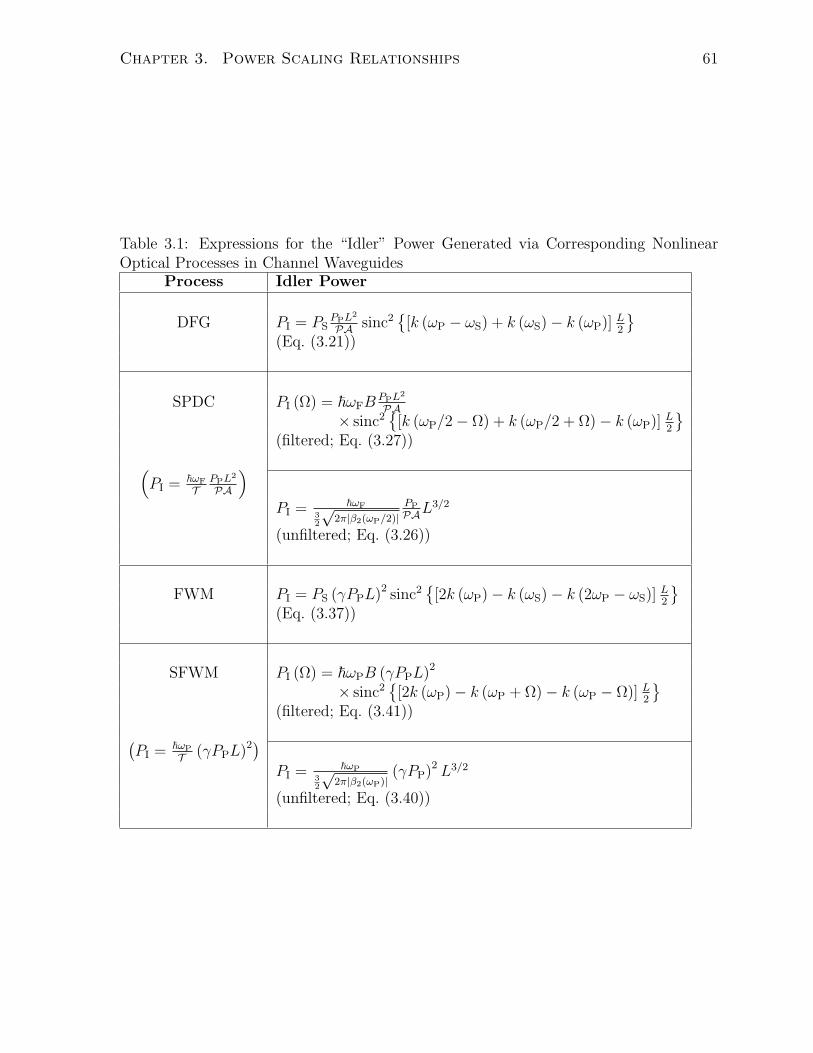
Chapter 3. Power Scaling Relationships 61
Table 3.1: Expressions for the “Idler” Power Generated via Corresponding NonlinearOptical Processes in Channel Waveguides
Process Idler Power
DFG PI = PSPPL
2
PA sinc2
[k (ωP − ωS) + k (ωS) − k (ωP)] L2
(Eq. (3.21))
SPDC PI (Ω) = ~ωFBPPL
2
PA× sinc2
[k (ωP/2 − Ω) + k (ωP/2 + Ω) − k (ωP)] L
2
(filtered; Eq. (3.27))(
PI = ~ωF
TPPL
2
PA
)PI = ~ωF
32
√2π|β2(ωP/2)|
PP
PAL3/2
(unfiltered; Eq. (3.26))
FWM PI = PS (γPPL)2 sinc2
[2k (ωP) − k (ωS) − k (2ωP − ωS)] L2
(Eq. (3.37))
SFWM PI (Ω) = ~ωPB (γPPL)2
× sinc2
[2k (ωP) − k (ωP + Ω) − k (ωP − Ω)] L2
(filtered; Eq. (3.41))(
PI = ~ωP
T (γPPL)2)
PI = ~ωP32
√2π|β2(ωP)|
(γPP)2 L3/2
(unfiltered; Eq. (3.40))
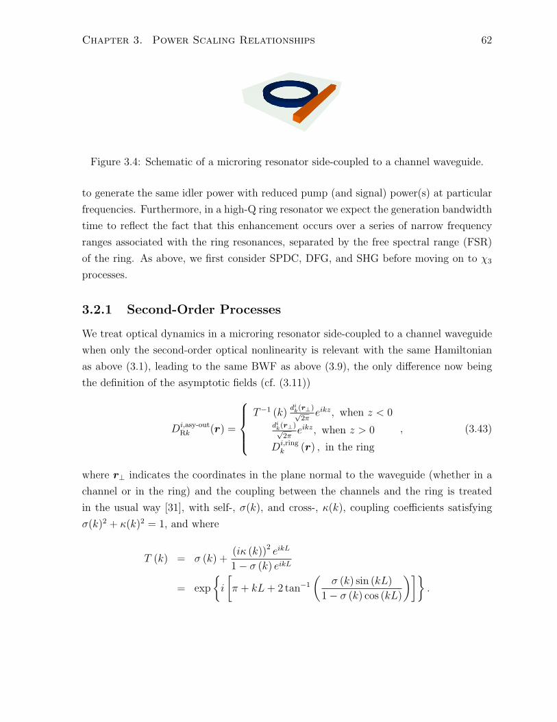
Chapter 3. Power Scaling Relationships 62
Figure 3.4: Schematic of a microring resonator side-coupled to a channel waveguide.
to generate the same idler power with reduced pump (and signal) power(s) at particular
frequencies. Furthermore, in a high-Q ring resonator we expect the generation bandwidth
time to reflect the fact that this enhancement occurs over a series of narrow frequency
ranges associated with the ring resonances, separated by the free spectral range (FSR)
of the ring. As above, we first consider SPDC, DFG, and SHG before moving on to χ3
processes.
3.2.1 Second-Order Processes
We treat optical dynamics in a microring resonator side-coupled to a channel waveguide
when only the second-order optical nonlinearity is relevant with the same Hamiltonian
as above (3.1), leading to the same BWF as above (3.9), the only difference now being
the definition of the asymptotic fields (cf. (3.11))
Di,asy-outRk (r) =
T−1 (k)
dik(r⊥)√2π
eikz, when z < 0dik(r⊥)√
2πeikz, when z > 0
Di,ringk (r) , in the ring
, (3.43)
where r⊥ indicates the coordinates in the plane normal to the waveguide (whether in a
channel or in the ring) and the coupling between the channels and the ring is treated
in the usual way [31], with self-, σ(k), and cross-, κ(k), coupling coefficients satisfying
σ(k)2 + κ(k)2 = 1, and where
T (k) = σ (k) +(iκ (k))2 eikL
1 − σ (k) eikL
= exp
i
[π + kL+ 2 tan−1
(σ (k) sin (kL)
1 − σ (k) cos (kL)
)].
Chapter 3. Power Scaling Relationships 63
The field in the ring is written as
Di,ringk (r) =
iκ(k)
1 − σ(k)eikLdik (r⊥, ζ/R)√
2πeikζ ,
where ζ is the coordinate in the counterclockwise direction along the ring circumference
of length L = 2πR, and ring resonances are described by k (ωm0)R = Nm with Nm ∈ Z.
While our formalism can treat nonlinear susceptibility tensors of general symmetry,
for instance rings made of III-V semiconductors in which there are unusual quasi-phase
matching conditions [2], for the sake of simplicity we here assume that the nonlinearity
experienced by the field of a ring mode remains constant as that field circles the ring. We
also assume that the fields involved are at frequencies near resonances, leading to strong
field enhancement due to constructive interference in the ring resonator and allowing
us to safely neglect any nonlinear effects outside the ring in the waveguide, where such
enhancement does not take place. To quantify how close the fields are to ring resonances,
consider first the example of SHG where we assume that (2k (ωF0) − k (ωSH0))R = 2NF−NSH = 0. For the frequencies ωF0 and ωSH0 , in general we will have ωSH0 = 2ωF0
because of dispersion, but we will assume that the fundamental and second harmonic
frequencies ωF and ωSH respectively, with ωSH = 2ωF, are characterized by detunings
δF(SH) = ωF(SH) − ωF0(SH0) so small that LδF(SH)/vF(SH) ≪ 1. Thus
ϕ (ω1, ω2) =iL
√dk (ω1)
dω1
√dk (ω2)
dω2
(√dk (ω)
dω
)ω=ω1+ω2
×
√ω1ω2 (χ2)
2NP
8πε0 |β|2 n6
√~ (ω1 + ω2)
A [k (ω1) , k (ω2) , k (ω1 + ω2)]
× ϕP (ω1 + ω2) sinc [k (ω1) + k (ω2) − k (ω1 + ω2)]L/2
× −iκ (k (ω1))
1 − σ(k (ω1))e−ik(ω1)L
−iκ (k (ω2))
1 − σ(k (ω2))e−ik(ω2)L
iκ(k (ω1 + ω2))
1 − σ(k (ω1 + ω2))eik(ω1+ω2)L,
(3.44)
and, for a CW pump of frequency ωP ≡ ωSH = ωSH0 , at a ring resonance, taking the
effective area, group velocities, and coupling terms κSH = κ (ωP), κF = κ (ωP/2), as
constant, we find that the average generated power associated with one photon of each
pair is
PI =~ωF
TPPL
2
PA|FP (ωP)|2 , (3.45)
Chapter 3. Power Scaling Relationships 64
with the generation bandwidth time being
T =2π/
(∫ ωP /2
0
dΩ[1 − (2Ω/ωP)2
]sinc [k (ωP/2 − Ω) + k (ωP/2 + Ω) − k (ωP)]L/2
× |FF (ωP/2 − Ω)|2 |FF (ωP/2 + Ω)|2),
provided PP ≪ PA/(L2 |FF (ωF0)|
3 |FP (ωP)|2)
(see (B.8)). Here P , A, PI, PP, and Ω
are as above (3.16), and the
Fm (ω) =iκm
1 − σmeik(ω)L,
are field enhancement factors. In the limit of no loss, these field enhancement factors
are equivalent to those defined in [3]. In particular, when the frequency is at a ring
resonance frequency, ω = ωm0 , we can write the enhancement factors in terms of the
quality factor(s) of the ring
Fm (ωm0) = 2i
√Qmvmωm0L
. (3.46)
Classical expressions follow easily from (3.18) using (3.43) for the asymptotic fields.
Employing a similar approach to the channel calculation above, a CW DFG calculation
yields
PI = PSPPL
2
PA|FS (ωS)|2 |FI (ωP − ωS)|2 |FP (ωP)|2 , (3.47)
whereas the SHG result is
PSH =P 2FL
2
PA|FF (ωF)|4 |FF (2ωF)|2 . (3.48)
We note that (3.48) was presented earlier [2], with consideration for arbitrary detuning
from resonance, for a GaAs ring resonator in which quasi-phase matching must be taken
into account.
We now turn to a comparison of the classical (stimulated) processes described by
(3.47) and (3.48), and the quantum (spontaneous) process described by (3.45). Note first
that, setting aside intensity enhancement factors, there is a quantum power ~ωF/T that
plays the role of the seed power PS in (3.47), analogous to what was seen in comparing
SPDC (3.16) with DFG (3.21) in a channel waveguide. For the structures considered
here there is an intensity enhancement factor for the pump |FP (ωP)|2 (two, resulting
in |FF (ωF)|4 in (3.48)) appearing in all three expressions (3.45), (3.47), and (3.48). In
Chapter 3. Power Scaling Relationships 65
the stimulated processes we also have intensity enhancement factors associated with
the signal input and idler output in (3.47), and with the second harmonic output in
(3.48). In (3.45), which describes an unseeded process, the frequency enhancement factors
associated with the generated fields reside in the generation bandwidth time T , and reflect
the fact that there is a range of frequencies over which the generated photons can appear.
Unlike in the channel calculation, looking only at photons generated within only a single
resonance near ωSH0/2, so that we may take
T ≈ 2π∫ ωP /2
0dΩ |FF (ωP/2 − Ω)|2 |FF (ωP/2 + Ω)|2
,
that time can be calculated here exactly, in the limit of small detuning and weak cou-
pling (σm ≈ 1), so that the intensity enhancement factors (i.e. absolute value of field
enhancement factors squared) become Lorentzians
|Fm (ω)|2 =κ2m
(1 − σm)2 + (ω − ωm0)2 (L/vm)2
,
and under the mild assumption that the integration range over the Lorentzians can be
extended to infinity without serious error. The result across a single resonance is
T =|FF (ωF0)|
4 L3 (2ωF0 − ωP)2 + 16v2FL
8v3F |FF (ωF0)|2 , (3.49)
where recall ωP = ωSH0 is the center frequency of the ring resonance at which the pump
frequency ωP is also centered, and ωF0 is the center frequency of the ring resonance in
which ωP/2 resides. We see that generation efficiency is worse the farther ωF0 is from
ωSH0/2. For ωF0 sufficiently close to ωSH0/2 we have
T =2L
vF |FF (ωF0)|2
=ωF0L
2
2v2FQF
, (3.50)
where we have used (3.46). We note that a similar result, albeit in a slightly different
form and calculated for a GaAs add/drop ring resonator instead of a ring resonator side-
coupled to a single channel waveguide, was previously presented [32]. Substituting (3.50)
Chapter 3. Power Scaling Relationships 66
in (3.45) we find
PI =~ωFvF
2L |FF (ωF0)|2
PPL2
PA|FP (ωP)|2 |FF0 (ωF0)|
4
=~ωF
QF
16πτF0
PPL2
PAQPvPωPL
(QFvFωF0L
)2
, (3.51)
where we have introduced τF0 = 2π/ωF0 . On the basis of (3.47) and (3.48), and the
fact the intensity enhancement factors |Fm (ωm0)|2 are proportional to the Qm (3.46),
one might have expected to see three quality factors in (3.51). However, because of the
resonance, the generation bandwidth time is also increased by a factor of QF and so there
are, in the end, only two that result.
Recall that we have assumed that all of the light is collected over a full ring resonance
linewidth. If one had a narrow enough filter with bandwidth 2πB that would select
out photons generated within just a small window of a ring resonance, the associated
calculation would yield
PI (Ω) =~ωF
B−1
PPL2
PA|FP (ωP)|2 |FF (ωP/2 − Ω)|2 |FF (ωP/2 + Ω)|2 , (3.52)
where Ω + ωP/2 now represents the center frequency of the accepted light.
It is worth noting that there is an entire frequency “comb” of resonances on either side
of half of the resonance being pumped that essentially satisfy both energy and momentum
conservation for the generated correlated photon pairs. Generation is significant up
until ωS0 + ωI0 − ωP0 (2ωF0 − ωP for the case considered above) becomes too large.
Quantifying this a bit more, the generation rate will be reduced by a factor of two
when ωS0 + ωI0 − ωP = 4vF/(|FF (ωF0)|
2 L)
= ωF0/QF (recall (3.49)). Taylor expanding
ωS0,I0 = ωF0 + vF (N −NF) /R + ΞF (N −NF)2 /R2, still taking 2ωF0 − ωP ≈ 0, and
remembering that if ωS0 is associated with resonance order N that ωI0 is associated with
resonance order NP −N , we find ωS0 + ωI0 − ωP0 = 2ΞF (N −NF)2 /R2. Thus, when
N −NF = R [ωF0/ (2 |ΞF|QF)]1/2 ,
the generation rate drops by a factor of two.
Armed with (3.47),(3.45), and (3.52), a classical (namely, DFG or SHG) experi-
ment that determines L2/ (PA) as well as the strength of a typical enhancement factor,
|FF (ωF0)|2, allows for an accurate prediction of the average power of photons generated
in a corresponding quantum experiment.
Chapter 3. Power Scaling Relationships 67
3.2.2 Third-Order Processes
As with the second order ring calculations, we can use the general expressions derived in
the Section on non-resonant structures to greatly simplify the calculations for a microring
resonator side-coupled to a channel waveguide. Starting with the same BWF as above
(3.30), and using the asymptotic fields appropriate for a microring resonator (3.43) we
find
ϕ (ω1, ω2) =3iL
√dk (ω1)
dω1
√dk (ω2)
dω2
∫ ω1+ω2
0
dω
[√dk (ω)
dω
(√dk (ω′)
dω′
)ω′=ω1+ω2−ω
×
√ω1ω2 (χ3)
2N 2P
128π2ε20 |β|2 n8
√~2ω (ω1 + ω2 − ω)
A2 [k (ω1) , k (ω2) , k (ω) , k (ω1 + ω2 − ω)]ϕP (ω)
× ϕP (ω1 + ω2 − ω) sinc [k (ω1) + k (ω2) − k (ω) − k (ω1 + ω2 − ω)]L/2
× −iκ (k (ω1))
1 − σ(k (ω1))e−ik(ω1)L
−iκ (k (ω2))
1 − σ(k (ω2))e−ik(ω2)L
× iκ(k (ω))
1 − σ(k (ω))eik(ω)Liκ(k (ω1 + ω2 − ω))
1 − σ(k (ω1 + ω2 − ω))eik(ω1+ω2−ω)L
], (3.53)
Assuming that the pump frequency ωP is at the center of one of the ring resonances,
ωP = ωP0 , and making the same approximation about integrating over the pump functions
as above (3.34), we find the average power associated with half of the generated photons
to be [33]
PI =~ωP
T(γPPL)2 |FP (ωP)|4 . (3.54)
We have also assumed that we are looking at photons generated within a pair of reso-
nances near enough to NP that we may take all group velocities, cross-sectional displace-
ment mode fields, resonant frequencies, and thus field enhancement factors to be those
of the pump, as well as the appropriate low-power limit (see (B.9)). The generation
bandwidth time is
T =2π∫ ωP
0dΩ |FP (ωP − Ω)|2 |FP (ωP + Ω)|2
.
Starting from (3.38), the corresponding CW FWM calculation yields
PI = PS (γPPL)2 |FP (ωP)|4 |FS (ωS)|2 |FI (2ωP − ωS)|2 , (3.55)
where γ is as above. We note that this expression agrees with a well-known result [3],
in the limit of no loss, small detuning, and weak coupling (σ ≈ 1). The comparison of
the classical (stimulated) process described by (3.55) with the quantum (spontaneous)
Chapter 3. Power Scaling Relationships 68
process described by (3.54) largely follows the comparison between (3.47) and (3.45)
respectively for second-order processes. Again we find that the generation bandwidth
time T can be calculated, with the result here given by
T =2L
vP |FP (ωP)|2
=ωPL
2
2v2PQP
, (3.56)
and thus, if photons are collected across an entire ring resonance linewidth, substituting
(3.56) in (3.54) we find
PI =~ωPvP
2L |FP (ωP)|2(γPPL)2 |FP (ωP)|8
=~ωP
QP
64πτP
(γPPL)2(QPvPωPL
)4
, (3.57)
where we have introduced τP = 2π/ωP. Note that the appearance of QP in the generation
bandwidth time leads to a net dependence of PI on three powers of QP, rather than the
four that might be expected from (3.55). If one had a filter with bandwidth 2πB, and
collected photons generated within just a small window of a ring resonance, one would
find instead
PI (Ω) =~ωP
B−1(γPPL)2 |FP (ωP)|4 |FP (ωP − Ω)|2 |FP (ωP + Ω)|2 , (3.58)
where Ω + ωP is the center of the narrow frequency window selected by the filter.
Once more there is an entire frequency comb of generated photons. Here the gener-
ation rate is reduced by a factor of two when ωS0 + ωI0 − 2ωP = 4vP/(|FP (ωP)|2 L
)=
ωP/QP. Taylor expanding as above while remembering that if ωS0 is associated with
resonance order N that ωI0 is associated with resonance order 2NP − N , we find that,
quite similar to above, when
N −NP = R [ωP/ (2 |ΞP|QP)]1/2 ,
the generation rate drops by a factor of two.
We conclude our analysis by summarizing in Tab. 3.2 all of the results for stimulated
and spontaneous processes in microring resonators. Here we report the “idler” powers as
a function of the quality factors Q and ring radius R, which are parameters that can be
easily measured and thus are experimentally used to characterize a device. These quan-
Chapter 3. Power Scaling Relationships 69
tities are directly related to the on-resonant intensity enhancement factors |FP (ωP)|2, as
such enhancement depends on the effective mode volume (∝ AR) as well as constructive
interference of the field in the ring, which is proportional to the time that light spends
in the resonator (proportional to Q).
Looking at the expressions reported in Tab. 3.2 we see that for DFG and SPDC, the
generated powers are inversely proportional to AR. Similarly, the generated idler powers
in FWM and SFWM scale with the inverse of (AR)2. In other words, the intensity
enhancement associated with the volume of the region in which light is confined has
the same weight, whether the process is spontaneous or stimulated. The situation is
different if we focus on the scaling of the generated powers with Q. In this case, unfiltered
SPDC and SFWM “ idler” powers are proportional to Q2 and Q3, respectively, while the
corresponding processes DFG and FWM scale with Q3 and Q4, respectively. Finally, as in
channel waveguides, stimulated and spontaneous powers scale the same when we consider
the spontaneous generated power in a sufficiently narrow spectral region centered at the
idler/signal resonance.
3.3 Experimental Verification
In response to our theoretical work, our experimental colleagues at the University of
Pavia, Italy, investigated the efficiencies of FWM and SFWM in silicon microring res-
onators as functions of pump power for various ring radii R and resonance quality factors
Q [18]. While not involved in the experiment I was involved in its analysis, and connected
some of the scaling expressions developed earlier in this Chapter with their results. This
Section summarizes that collaborative work. In particular the expressions (3.55) and
(3.57) are investigated, as is the ratio between them.
3.3.1 Set Up
The resonators under investigation were fabricated on a silicon-on-insulator (SOI) wafer
via e-beam lithography and inductively coupled plasma etching. Rings with radii of 5,
10, 20, and 30 µm were side-coupled to a bus waveguide. The waveguides and rings
have a 220 × 500 nm2 rectangular cross section. Spot-size converters were used for
efficient coupling [68]. The silicon chip was finally coated with a protective polymethyl
methacrylate (PMMA) layer.
The samples’ linear properties were characterized using a swept laser. As an example,
the transmission curve for the R = 5 µm ring is shown in Fig. 3.5. The spectrum shows
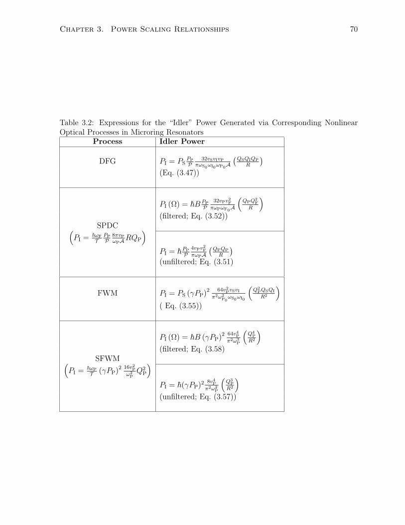
Chapter 3. Power Scaling Relationships 70
Table 3.2: Expressions for the “Idler” Power Generated via Corresponding NonlinearOptical Processes in Microring Resonators
Process Idler Power
DFG PI = PSPP
P32vSvIvP
πωS0ωI0
ωP0A
(QSQIQP
R
)(Eq. (3.47))
PI (Ω) = ~B PP
P32vPv
2F
πωPωF0A
(QPQ
2F
R
)(filtered; Eq. (3.52))
SPDC(PI = ~ωF
TPP
P8πvPωPA
RQP
)PI = ~PP
P4vPv
2F
πωPA
(QFQP
R
)(unfiltered; Eq. (3.51)
FWM PI = PS (γPP)264v2PvSvI
π2ω2P0
ωS0ωI0
(Q2
PQSQI
R2
)( Eq. (3.55))
PI (Ω) = ~B (γPP)264v4Pπ2ω3
P
(Q4
P
R2
)(filtered; Eq. (3.58)
SFWM(PI = ~ωP
T (γPP)216v2Pω2PQ2
P
)PI = ~(γPP)2
8v4Pπ2ω2
P
(Q3
P
R2
)(unfiltered; Eq. (3.57))
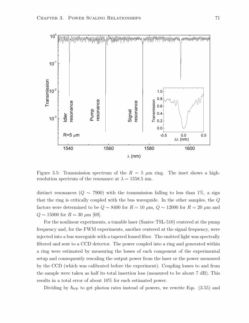
Chapter 3. Power Scaling Relationships 71
-0.5 0.0 0.5
0.0
0.2
0.4
0.6
0.8
1.0
1540 1560 1580 1600
10-3
10-2
10-1
100
(nm)
Sign
alre
sona
nce
Idle
rre
sona
nce
R=5 m
Tran
smis
sion
Pum
pre
sona
nce
Tra
nsm
issi
on
(nm)
Figure 3.5: Transmission spectrum of the R = 5 µm ring. The inset shows a high-resolution spectrum of the resonance at λ = 1558.5 nm.
distinct resonances (Q ∼ 7900) with the transmission falling to less than 1%, a sign
that the ring is critically coupled with the bus waveguide. In the other samples, the Q
factors were determined to be Q ∼ 8400 for R = 10 µm, Q ∼ 12000 for R = 20 µm and
Q ∼ 15000 for R = 30 µm [69].
For the nonlinear experiments, a tunable laser (Santec TSL-510) centered at the pump
frequency and, for the FWM experiments, another centered at the signal frequency, were
injected into a bus waveguide with a tapered lensed fiber. The emitted light was spectrally
filtered and sent to a CCD detector. The power coupled into a ring and generated within
a ring were estimated by measuring the losses of each component of the experimental
setup and consequently rescaling the output power from the laser or the power measured
by the CCD (which was calibrated before the experiment). Coupling losses to and from
the sample were taken as half its total insertion loss (measured to be about 7 dB). This
results in a total error of about 10% for each estimated power.
Dividing by ~ωP to get photon rates instead of powers, we rewrite Eqs. (3.55) and
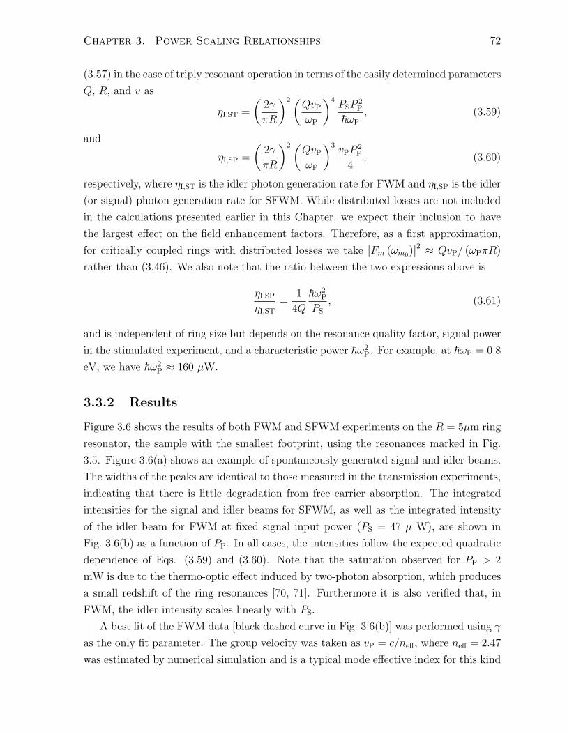
Chapter 3. Power Scaling Relationships 72
(3.57) in the case of triply resonant operation in terms of the easily determined parameters
Q, R, and v as
ηI,ST =
(2γ
πR
)2(QvPωP
)4PSP
2P
~ωP
, (3.59)
and
ηI,SP =
(2γ
πR
)2(QvPωP
)3vPP
2P
4, (3.60)
respectively, where ηI,ST is the idler photon generation rate for FWM and ηI,SP is the idler
(or signal) photon generation rate for SFWM. While distributed losses are not included
in the calculations presented earlier in this Chapter, we expect their inclusion to have
the largest effect on the field enhancement factors. Therefore, as a first approximation,
for critically coupled rings with distributed losses we take |Fm (ωm0)|2 ≈ QvP/ (ωPπR)
rather than (3.46). We also note that the ratio between the two expressions above is
ηI,SPηI,ST
=1
4Q
~ω2P
PS
, (3.61)
and is independent of ring size but depends on the resonance quality factor, signal power
in the stimulated experiment, and a characteristic power ~ω2P. For example, at ~ωP = 0.8
eV, we have ~ω2P ≈ 160 µW.
3.3.2 Results
Figure 3.6 shows the results of both FWM and SFWM experiments on the R = 5µm ring
resonator, the sample with the smallest footprint, using the resonances marked in Fig.
3.5. Figure 3.6(a) shows an example of spontaneously generated signal and idler beams.
The widths of the peaks are identical to those measured in the transmission experiments,
indicating that there is little degradation from free carrier absorption. The integrated
intensities for the signal and idler beams for SFWM, as well as the integrated intensity
of the idler beam for FWM at fixed signal input power (PS = 47 µ W), are shown in
Fig. 3.6(b) as a function of PP. In all cases, the intensities follow the expected quadratic
dependence of Eqs. (3.59) and (3.60). Note that the saturation observed for PP > 2
mW is due to the thermo-optic effect induced by two-photon absorption, which produces
a small redshift of the ring resonances [70, 71]. Furthermore it is also verified that, in
FWM, the idler intensity scales linearly with PS.
A best fit of the FWM data [black dashed curve in Fig. 3.6(b)] was performed using γ
as the only fit parameter. The group velocity was taken as vP = c/neff, where neff = 2.47
was estimated by numerical simulation and is a typical mode effective index for this kind
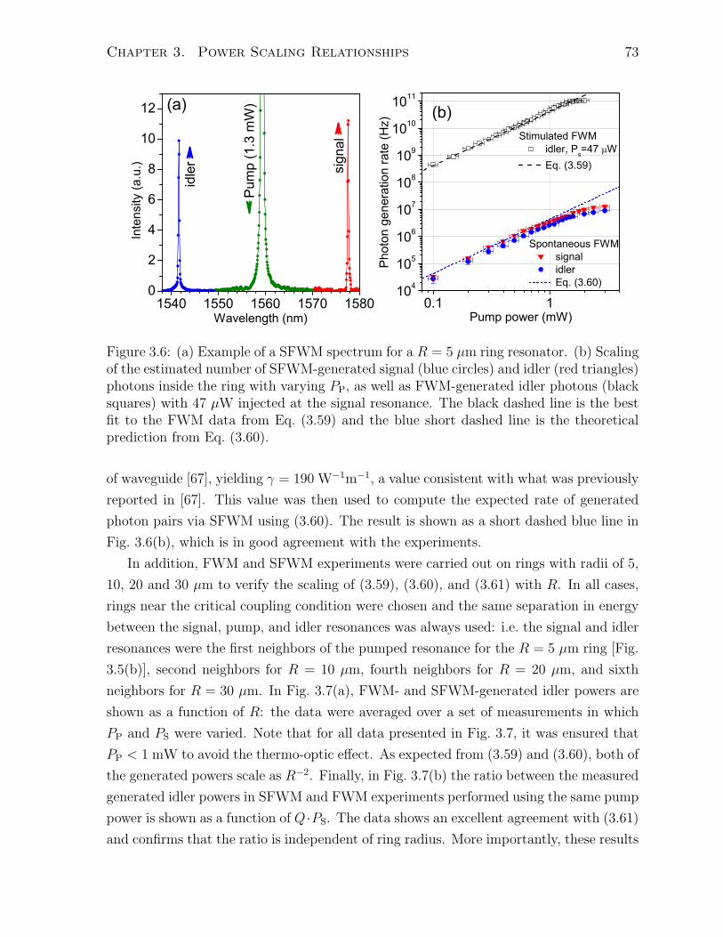
Chapter 3. Power Scaling Relationships 73
1540 1550 1560 1570 15800
2
4
6
8
10
12
0.1 1104
105
106
107
108
109
1010
1011
(b)
Pum
p (1
.3 m
W)
sign
al
Inte
nsity
(a.u
.)
Wavelength (nm)
idle
r
(a)
Spontaneous FWM signal idler Eq. (3.60)
Stimulated FWM idler, Ps=47 W Eq. (3.59)
Pho
ton
gene
ratio
n ra
te (H
z)
Pump power (mW)
Figure 3.6: (a) Example of a SFWM spectrum for a R = 5 µm ring resonator. (b) Scalingof the estimated number of SFWM-generated signal (blue circles) and idler (red triangles)photons inside the ring with varying PP, as well as FWM-generated idler photons (blacksquares) with 47 µW injected at the signal resonance. The black dashed line is the bestfit to the FWM data from Eq. (3.59) and the blue short dashed line is the theoreticalprediction from Eq. (3.60).
of waveguide [67], yielding γ = 190 W−1m−1, a value consistent with what was previously
reported in [67]. This value was then used to compute the expected rate of generated
photon pairs via SFWM using (3.60). The result is shown as a short dashed blue line in
Fig. 3.6(b), which is in good agreement with the experiments.
In addition, FWM and SFWM experiments were carried out on rings with radii of 5,
10, 20 and 30 µm to verify the scaling of (3.59), (3.60), and (3.61) with R. In all cases,
rings near the critical coupling condition were chosen and the same separation in energy
between the signal, pump, and idler resonances was always used: i.e. the signal and idler
resonances were the first neighbors of the pumped resonance for the R = 5 µm ring [Fig.
3.5(b)], second neighbors for R = 10 µm, fourth neighbors for R = 20 µm, and sixth
neighbors for R = 30 µm. In Fig. 3.7(a), FWM- and SFWM-generated idler powers are
shown as a function of R: the data were averaged over a set of measurements in which
PP and PS were varied. Note that for all data presented in Fig. 3.7, it was ensured that
PP < 1 mW to avoid the thermo-optic effect. As expected from (3.59) and (3.60), both of
the generated powers scale as R−2. Finally, in Fig. 3.7(b) the ratio between the measured
generated idler powers in SFWM and FWM experiments performed using the same pump
power is shown as a function of Q·PS. The data shows an excellent agreement with (3.61)
and confirms that the ratio is independent of ring radius. More importantly, these results
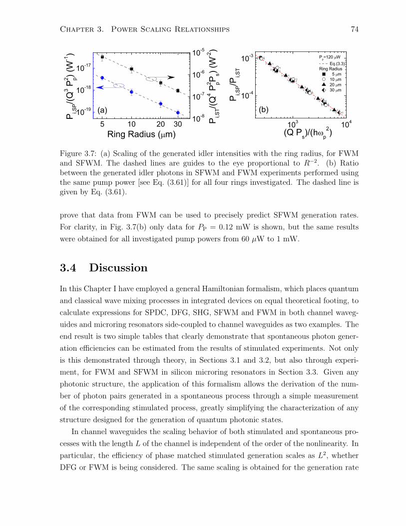
Chapter 3. Power Scaling Relationships 74
5 10 20 3010-19
10-18
10-17
103 104
10-4
10-3
P i,SP/(Q
3 P2 p) (
W-1)
Ring Radius ( m)
10-8
10-7
10-6
10-5
Pi,S
T/(Q4 P
2 pP s) (W
-2)
(b)(a)
Pp=120 W Eq.(3.3)
Ring Radius 5 m 10 m 20 m 30 m
P i,SP/P
i,ST
(Q Ps)/(h p2)
Figure 3.7: (a) Scaling of the generated idler intensities with the ring radius, for FWMand SFWM. The dashed lines are guides to the eye proportional to R−2. (b) Ratiobetween the generated idler photons in SFWM and FWM experiments performed usingthe same pump power [see Eq. (3.61)] for all four rings investigated. The dashed line isgiven by Eq. (3.61).
prove that data from FWM can be used to precisely predict SFWM generation rates.
For clarity, in Fig. 3.7(b) only data for PP = 0.12 mW is shown, but the same results
were obtained for all investigated pump powers from 60 µW to 1 mW.
3.4 Discussion
In this Chapter I have employed a general Hamiltonian formalism, which places quantum
and classical wave mixing processes in integrated devices on equal theoretical footing, to
calculate expressions for SPDC, DFG, SHG, SFWM and FWM in both channel waveg-
uides and microring resonators side-coupled to channel waveguides as two examples. The
end result is two simple tables that clearly demonstrate that spontaneous photon gener-
ation efficiencies can be estimated from the results of stimulated experiments. Not only
is this demonstrated through theory, in Sections 3.1 and 3.2, but also through experi-
ment, for FWM and SFWM in silicon microring resonators in Section 3.3. Given any
photonic structure, the application of this formalism allows the derivation of the num-
ber of photon pairs generated in a spontaneous process through a simple measurement
of the corresponding stimulated process, greatly simplifying the characterization of any
structure designed for the generation of quantum photonic states.
In channel waveguides the scaling behavior of both stimulated and spontaneous pro-
cesses with the length L of the channel is independent of the order of the nonlinearity. In
particular, the efficiency of phase matched stimulated generation scales as L2, whether
DFG or FWM is being considered. The same scaling is obtained for the generation rate
Chapter 3. Power Scaling Relationships 75
of spontaneous processes within a sufficiently narrow spectral region around the phase
matching condition. Similarly, the generated idler power, integrated over the entire
spectrum, scales with L3/2 for both SPDC and SFWM in a channel, as in the absence of
filtering the generation bandwidth time scales as L1/2. This is in contrast with the results
for a microring resonator, in which all second order processes scale with ring radius R as
R−1 and all third-order processes as R−2 regardless of filtering. Considering enhancement
due to light confinement in the channel, which is inversely proportional to the effective
area, one sees that this effect on the generated power is independent of the nature of the
process, stimulated or spontaneous, while it depends upon the order of the nonlinearity.
Indeed, for DFG and SPDC, the generation rate is proportional to 1/A, while for FWM
and SFWM it scales with γ2 ∝ 1/A2. This result is consistent with the fact that for
the example of a channel the scaling with L is due solely to the interference of the fields
generated at different positions in the channel. That is, there is no L-dependent field
enhancement. Again this is in contrast with the results for a microring side-coupled to a
channel waveguide, in which the additional confinement in the direction of propagation
due to the ring plays a role. DFG and FWM scale with Q3 and Q4, respectively, in a
ring resonator as do the corresponding spontaneous processes within a sufficiently nar-
row spectral region centered at the idler/signal resonance. Unfiltered SPDC and SFWM
generated powers, on the other hand, are proportional to Q2 and Q3, respectively.
Chapter 4
Biphoton Engineering
Not all photons are created equal, nor should they be. Different applications demand
quantum correlated photon pairs with different properties. For example, maximal vio-
lation of Bell’s inequality [6, 7] using polarization entangled photons requires only that
both photons of a given pair have the same marginal frequency distribution, whereas
entanglement swapping of polarization entangled photon pairs may be spoiled by any
sort of frequency correlations [42]. Further, interaction with various other systems (e.g.
quantum memories) necessitates the generation of photons with specific frequency band-
widths. Thus, in addition to predicting the rate of pair generation, as in the previous
Chapter, it is also important to understand the range of possible quantum correlated
states of photon pairs that can be generated in various artificially structured media.
In this Chapter I examine the general form of the biphoton probability density∣∣∣ϕC(R)2(3)µν (ω1, ω2)
∣∣∣2 ,associated with photons generated in each a channel waveguide, C, and a microring res-
onator side-coupled to a channel waveguide, R, via a second- or third-order nonlinearity,
denoted by 2 and 3 respectively, as well as the parameters that need to be adjusted in or-
der to achieve a particular shape of the biphoton probability density for each nonlinearity
in each structure. The Greek subscripts, while not used in the previous Chapter, label
the generated photon mode-types (i.e. they are the I’s in (2.26)), and will be discussed
further in the following Section. While similar idealized theoretical investigations have
been carried out previously, such as how to create frequency uncorrelated photon pairs
via type-II (defined in Section 4.1) SPDC in bulk crystals [72] as well as in Bragg reflec-
tion waveguides [73], how to create maximally polarization-entangled photons via SPDC
in Bragg reflection waveguides [74], an analysis of the performance of bulk crystal SPDC-
76
Chapter 4. Biphoton Engineering 77
generated photon pairs in entanglement swapping gates and type-I fusion gates [42], and
the optimization of SPDC-generated photons for quantum information processing [40],
here the scope is grander. The widths of biphoton probability densities associated with
photon pairs generated via not only type-I or type-II SPDC, but also type-I or type-II
SFWM, and not only generated in channel waveguides, but also generated in microring
resonators, are catalogued such that approximate analytic expressions for the Schmidt
numbers [63] of the associated BWFs can be easily obtained, and suitability of the vari-
ous photon pairs for two specific applications can be easily quantified. It is demonstrated
that the shape of the biphoton probability density depends strongly on dispersion for
a channel waveguide, and strongly on coupling between the ring and the waveguide for
a microring resonator. This second fact presents a novel way to realize the efficient
generation of uncorrelated photons on a chip.
In Section 4.1 general expressions for the state of generated photons from a SPDC or
SFWM process in either a channel waveguide or microring resonator as well as their asso-
ciated BWFs are presented. We do not consider any phase accumulated by the generated
photons on their way to a detector, or even while propagating in the nonlinear material
itself, as it can, at least in principle, be compensated for by an opposite-signed dispersive
element. As application examples, in Section 4.2 we discuss CHSH inequality violation
[7] and entanglement swapping [42], corresponding to a classic single photon pair source
application and multi-source application respectively, with consideration given to how
the BWF influences each. In Section 4.3 possible associated biphoton probability densi-
ties, centered at the origin, are explored, along with approximate analytic expressions for
their widths. These expressions are in terms of pump and photon pair source parameters,
providing a method to engineer the correlations in the biphoton probability density nec-
essary for successful implementation of one of the aforementioned applications through
careful waveguide design and choice of pump pulse bandwidth. A more quantitative
analysis focusing on the Schmidt number is presented in Section 4.4, where a comparison
is made with double-Gaussian BWFs, for which the Schmidt number can be calculated
analytically, and in Section 4.5 a discussion of these results follows.
As in the previous Chapter, here all nonlinear effects other than SPDC or SFWM are
neglected, the results presented are only strictly valid in the undepleted pump approxi-
mation at low enough pump powers, and all forms of loss are neglected as well. While
it is true that the BWF associated with a photon pair source in the lab may not meet
all of these idealizations, it is also true that if an idealized source is not suitable for a
particular application then any non-idealizations will certainly not improve its suitability.
Therefore the results of this Chapter can be thought of as source design guidelines, if not
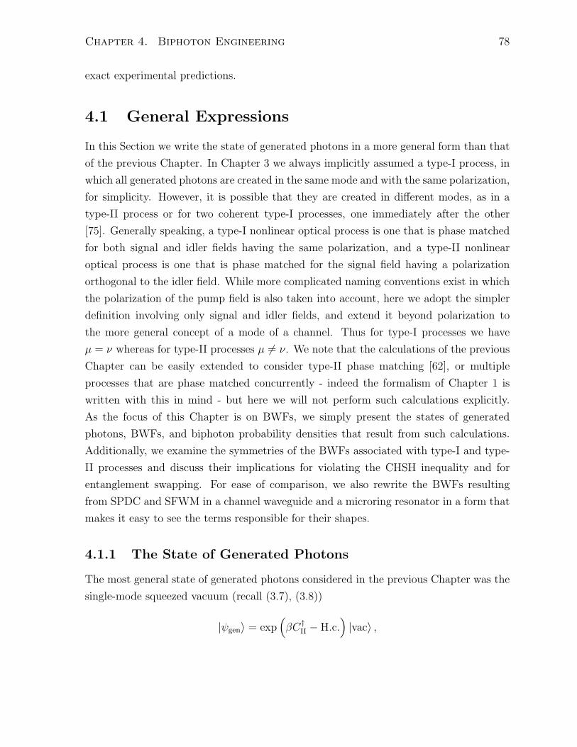
Chapter 4. Biphoton Engineering 78
exact experimental predictions.
4.1 General Expressions
In this Section we write the state of generated photons in a more general form than that
of the previous Chapter. In Chapter 3 we always implicitly assumed a type-I process, in
which all generated photons are created in the same mode and with the same polarization,
for simplicity. However, it is possible that they are created in different modes, as in a
type-II process or for two coherent type-I processes, one immediately after the other
[75]. Generally speaking, a type-I nonlinear optical process is one that is phase matched
for both signal and idler fields having the same polarization, and a type-II nonlinear
optical process is one that is phase matched for the signal field having a polarization
orthogonal to the idler field. While more complicated naming conventions exist in which
the polarization of the pump field is also taken into account, here we adopt the simpler
definition involving only signal and idler fields, and extend it beyond polarization to
the more general concept of a mode of a channel. Thus for type-I processes we have
µ = ν whereas for type-II processes µ = ν. We note that the calculations of the previous
Chapter can be easily extended to consider type-II phase matching [62], or multiple
processes that are phase matched concurrently - indeed the formalism of Chapter 1 is
written with this in mind - but here we will not perform such calculations explicitly.
As the focus of this Chapter is on BWFs, we simply present the states of generated
photons, BWFs, and biphoton probability densities that result from such calculations.
Additionally, we examine the symmetries of the BWFs associated with type-I and type-
II processes and discuss their implications for violating the CHSH inequality and for
entanglement swapping. For ease of comparison, we also rewrite the BWFs resulting
from SPDC and SFWM in a channel waveguide and a microring resonator in a form that
makes it easy to see the terms responsible for their shapes.
4.1.1 The State of Generated Photons
The most general state of generated photons considered in the previous Chapter was the
single-mode squeezed vacuum (recall (3.7), (3.8))
|ψgen⟩ = exp(βC†
II − H.c.)|vac⟩ ,
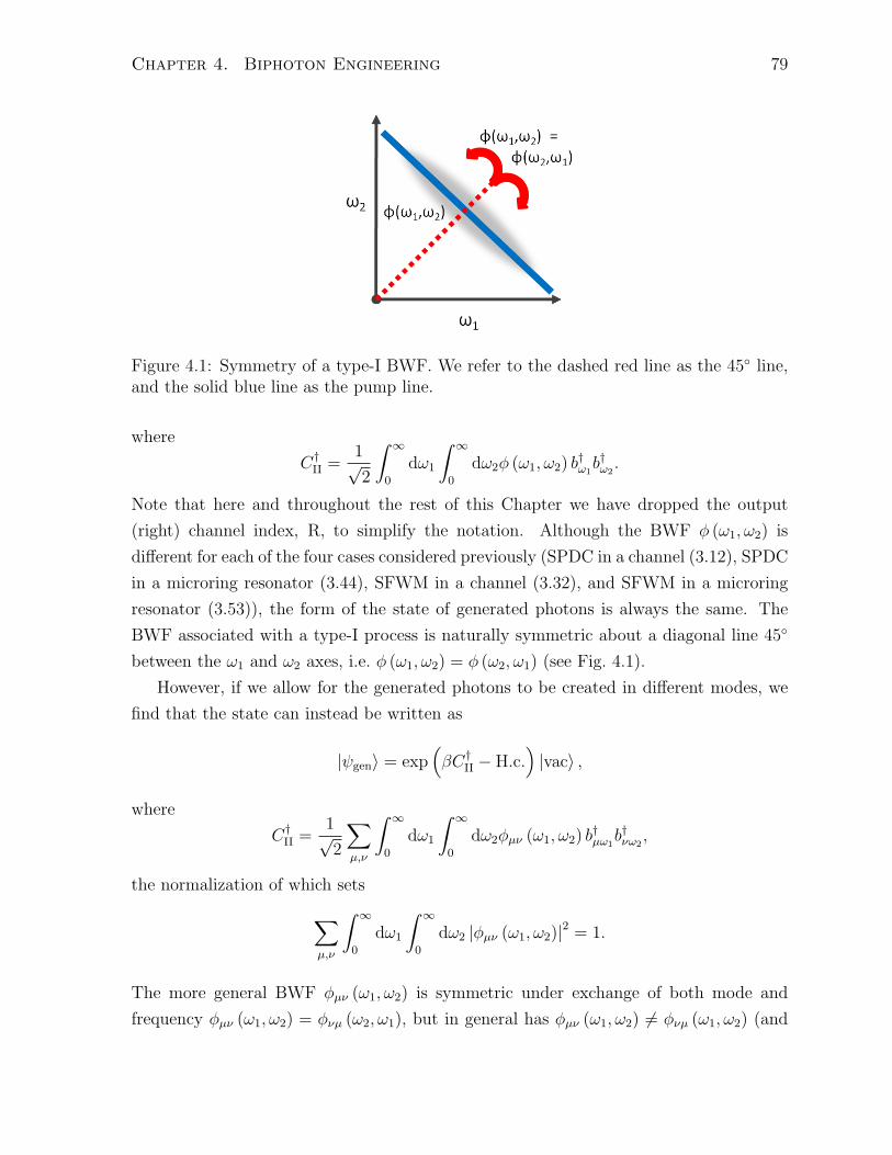
Chapter 4. Biphoton Engineering 79
Figure 4.1: Symmetry of a type-I BWF. We refer to the dashed red line as the 45 line,and the solid blue line as the pump line.
where
C†II =
1√2
∫ ∞
0
dω1
∫ ∞
0
dω2ϕ (ω1, ω2) b†ω1b†ω2.
Note that here and throughout the rest of this Chapter we have dropped the output
(right) channel index, R, to simplify the notation. Although the BWF ϕ (ω1, ω2) is
different for each of the four cases considered previously (SPDC in a channel (3.12), SPDC
in a microring resonator (3.44), SFWM in a channel (3.32), and SFWM in a microring
resonator (3.53)), the form of the state of generated photons is always the same. The
BWF associated with a type-I process is naturally symmetric about a diagonal line 45
between the ω1 and ω2 axes, i.e. ϕ (ω1, ω2) = ϕ (ω2, ω1) (see Fig. 4.1).
However, if we allow for the generated photons to be created in different modes, we
find that the state can instead be written as
|ψgen⟩ = exp(βC†
II − H.c.)|vac⟩ ,
where
C†II =
1√2
∑µ,ν
∫ ∞
0
dω1
∫ ∞
0
dω2ϕµν (ω1, ω2) b†µω1b†νω2
,
the normalization of which sets∑µ,ν
∫ ∞
0
dω1
∫ ∞
0
dω2 |ϕµν (ω1, ω2)|2 = 1.
The more general BWF ϕµν (ω1, ω2) is symmetric under exchange of both mode and
frequency ϕµν (ω1, ω2) = ϕνµ (ω2, ω1), but in general has ϕµν (ω1, ω2) = ϕνµ (ω1, ω2) (and

Chapter 4. Biphoton Engineering 80
thus ϕµν (ω1, ω2) = ϕµν (ω2, ω1)). More specifically the dispersion relation, or dependence
of k on ω, is not necessarily the same for each of the fields involved, meaning that this
type of BWF is not, in general, symmetric about a diagonal line 45 between the ω1 and
ω2 axes (see Fig. 4.1). We refer to this line as the 45 line, and a line perpendicular to
it and passing through the center of the BWF as the pump line.
Focusing on polarization modes (horizontal, H, and vertical, V) only, note that while
|ψHVVH⟩ ∝1√2
∫ ∞
0
dω1
∫ ∞
0
dω2
[ϕHV (ω1, ω2) b
†Hω1
b†Vω2+ ϕVH (ω1, ω2) b
†Vω1
b†Hω2
]|vac⟩ ,
(4.1)
should be written as such to make its symmetric nature explicit, it could just as easily
be written as
|ψHVVH⟩ ∝√
2
∫ ∞
0
dω1
∫ ∞
0
dω2ϕHV (ω1, ω2) b†Hω1
b†Vω2|vac⟩ ,
i.e. all of the information about the correlations between the two photons is contained
within a single function with fixed polarization indices ϕHV (ω1, ω2), and the other piece
of the total BWF ϕVH (ω1, ω2) can be calculated from symmetry arguments. This is why
often only a single function with fixed polarization indices is plotted in the literature [27].
However the same is not true for a state such as
|ψHHVV⟩ ∝1√2
∫ ∞
0
dω1
∫ ∞
0
dω2
[ϕHH (ω1, ω2) b
†Hω1
b†Hω2+ ϕVV (ω1, ω2) b
†Vω1
b†Vω2
]|vac⟩ .
(4.2)
Furthermore, symmetry arguments ensure that, for the state |ψHVVH⟩ (4.1),∫ ∞
0
dω1
∫ ∞
0
dω2 |ϕHV (ω1, ω2)|2 =
∫ ∞
0
dω1
∫ ∞
0
dω2 |ϕVH (ω1, ω2)|2 = 1/2,
whereas while∫ ∞
0
dω1
∫ ∞
0
dω2 |ϕHH (ω1, ω2)|2 +
∫ ∞
0
dω1
∫ ∞
0
dω2 |ϕVV (ω1, ω2)|2 = 1,
for the state |ψHHVV⟩ (4.2), it is not necessary that they are both equal.
4.1.2 The Biphoton Wave Function
As we are concerned with the shape of the absolute value squared of each of these two-
dimensional functions here, we rewrite each in a form that highlights the pieces with the
greatest influence on their shape. Whether photon pair generation occurs due to a SPDC
Chapter 4. Biphoton Engineering 81
process in a channel waveguide or in a microring resonator, the resulting BWF has the
same general form (cf. (3.12), (3.44))
ϕC2µν (ω1, ω2) = BC2
µν (ω1, ω2)ϕP (ω1 + ω2) θC2µν (ω1, ω2) ,
ϕR2µν (ω1, ω2) = BR2
µν (ω1, ω2)ϕP (ω1 + ω2) θR2µν (ω1, ω2) . (4.3)
Here
BC2µν (ω1, ω2) =iL
√dkµ (ω1)
dω1
√dkν (ω2)
dω2
(√dkP (ω)
dω
)ω=ω1+ω2
×
√ω1ω2 (χ2)
2 NP
8πε0 |β|2 n6
√~ (ω1 + ω2)
A [kµ (ω1) , kν (ω2) , kP (ω1 + ω2)],
and
BR2µν (ω1, ω2) = − iBC2
µν (ω1, ω2) sinc [kµ (ω1) + kν (ω2) − kP (ω1 + ω2)]L/2
× κµκνκPvµvνvP/L3
are benign functions of generated photon frequencies, or functions which have little influ-
ence over the shape of the biphoton probability density, i.e. they are essentially constant
over the range over which the product of the other two functions is significantly nonzero.
Additionally A is an effective area for the nonlinear process (see (3.13)), ϕP (ω) the
pump pulse waveform, and κ (with κ2 + σ2 = 1) the cross-coupling coefficient between
bus waveguide and ring, with σ the self-coupling coefficient. Note that the phase match-
ing sinc function is included in the benign function for SPDC in a microring resonator
BR2µν (ω1, ω2), as here we are assuming that the center frequencies of the three fields in-
volved are on resonance and that these resonances are narrow enough that the squared
sinc function appearing in the biphoton probability density is approximately unity over
a resonance linewidth. That is, for some ωµ + ων = ωP, set so that km (ωm)L = 2πNm,
with Nm an integer for m = µ, ν or P, we have kµ (ωµ) + kν (ων) = kP (ωP). Thus when
Fm (ω) =iκ (km (ω))
1 − σ(km (ω))eikm(ω)L
≈ iκmvm/L
Ωm − i (ω − ωm),
is a reasonable approximation for all three resonances, where we have defined κ (km (ωm)) ≡κm, σ (km (ωm)) ≡ σm, Ωm = (1 − σm) vm/L and assumed weak coupling, σm ≈ 1, we find

Chapter 4. Biphoton Engineering 82
kµ (ω1) + kν (ω2) − kP (ω1 + ω2) ≈ kµ (ωµ) + kν (ων) − kP (ωµ + ων) = 0. The quantity Ω
can also be thought of as half the full-width at half-maximum (FWHM) of the resonance
linewidth, and is related to the quality factor Q via Ωm = ωm/ (2Qm). Furthermore we
take
ϕP (ω) =exp
(− (ω − ωP )2 / (2∆2
ω))(√
2π∆ω
)1/2 ,
as the pump waveform - a function of the sum of generated photon frequencies - and
θC2µν (ω1, ω2) = sinc [kµ (ω1) + kν (ω2) − kP (ω1 + ω2)]L/2 ,
θR2µν (ω1, ω2) = [Ωµ + i (ω1 − ωµ)]−1 [Ων + i (ω2 − ων)]−1 [ΩP − i (ω1 + ω2 − ωP)]−1 ,
are more complicated functions of the generated photon frequencies.
Similarly, for SFWM, taking ωµ + ων = 2ωP, so that kµ (ωµ) + kν (ων) = 2kP (ωP), we
have (cf. (3.32), (3.53))
ϕC3µν (ω1, ω2) = BC3
µν (ω1, ω2) θC3µν (ω1, ω2) ,
ϕR3µν (ω1, ω2) = BR3
µν (ω1, ω2) θR3µν (ω1, ω2) , (4.4)
with
BC3µν (ω1, ω2) ≈3iL
√dkµ (ω1)
dω1
√dkν (ω2)
dω2
√ω1ω2 (χ3)
2 N 2P
128π2ε20 |β|2 n8
×
(√dkP (ω)
dω
∣∣∣∣∣ω=ωP
)2√~2ω2
P
A2 [kµ (ω1) , kν (ω2) , kP (ωP) , kP (ωP)],
BR3µν (ω1, ω2) ≈BC3
µν (ω1, ω2) sinc [kµ (ω1) + kν (ω2) − 2kP (ωP)]L/2
× κµκνκ2Pvµvνv
2P/L
4
as well as
θC3µν (ω1, ω2) =
∫ ω1+ω2
0
dω (ϕP (ω)ϕP (ω1 + ω2 − ω)
× sinc [kµ (ω1) + kν (ω2) − kP (ω) − kP (ω1 + ω2 − ω)]L/2) ,
Chapter 4. Biphoton Engineering 83
θR3µν (ω1, ω2) =
∫ ω1+ω2
0
dωϕP (ω)ϕP (ω1 + ω2 − ω) [Ωµ + i (ω1 − ωµ)]−1 [Ων + i (ω2 − ων)]−1
× [ΩP − i (ω − ωP)]−1 [ΩP − i (ω1 + ω2 − ω − ωP)]−1 ,if we assume that the group velocities, coupling constants, effective area (see (3.33)), and
sinc function are also essentially constant over the integral over ω. Note that, unlike for
SPDC, θC3µν (ω1, ω2) and θR3
µν (ω1, ω2) contain integrals over the pump waveform. This is
because two pump photons are annihilated in a SFWM process, and energy conservation
alone, expressed by a Dirac delta function in our formalism (recall (3.6)), is not enough
to set the frequency of each generated photon in relation to more than one pump photon.
4.2 Single-Source vs. Multi-Source Experiments
Again focusing on just polarization modes for simplicity, we imagine an idealized state
preparation in which a single pair of photons of the type (4.1) or (4.2) is separated with
a 50/50 beam-splitter, and then directed to an appropriate set of polarization beam-
splitters and phase delays to become one of the four states [76]
∣∣Ψ±⟩12
=1√2
∫ ∞
0
dω1
∫ ∞
0
dω2 [ϕHV (ω1, ω2) |H (ω1) V (ω2)⟩12
± ϕVH (ω1, ω2) |V (ω1) H (ω2)⟩12] , (4.5)
∣∣Φ±⟩12
=1√2
∫ ∞
0
dω1
∫ ∞
0
dω2 [ϕHH (ω1, ω2) |H (ω1) H (ω2)⟩12
± ϕVV (ω1, ω2) |V (ω1) V (ω2)⟩12] , (4.6)
where |A (ω1)B (ω2)⟩12 = b†Aω1;1b†Bω2;2
|vac⟩, the additional labels 1 and 2 indicating which
beam-splitter port the photon exited. While half of the time the photons will both end
up exiting the same 50/50 beam-splitter port, these events are simply ignored here in our
idealized picture of possible photon pair sources. Alternatively, a similar effect could be
obtained with a dichroic beam-splitter without taking a 3dB penalty [74]. As the two pho-
tons now exist in separate channels and some have been neglected, the BWFs should be
renormalized such that∫∞0
dω1
∫∞0
dω2 |ϕHV (ω1, ω2)|2 =∫∞0
dω1
∫∞0
dω2 |ϕVH (ω1, ω2)|2 =
1, and∫∞0
dω1
∫∞0
dω2 |ϕHH (ω1, ω2)|2 +∫∞0
dω1
∫∞0
dω2 |ϕVV (ω1, ω2)|2 = 2. Note that such
a renormalization does not affect any of the θC(R)2(3)µν (ω1, ω2) or ϕP (ω) functions that de-
termine the shape of the various BWFs, but simply introduces a multiplicative constant
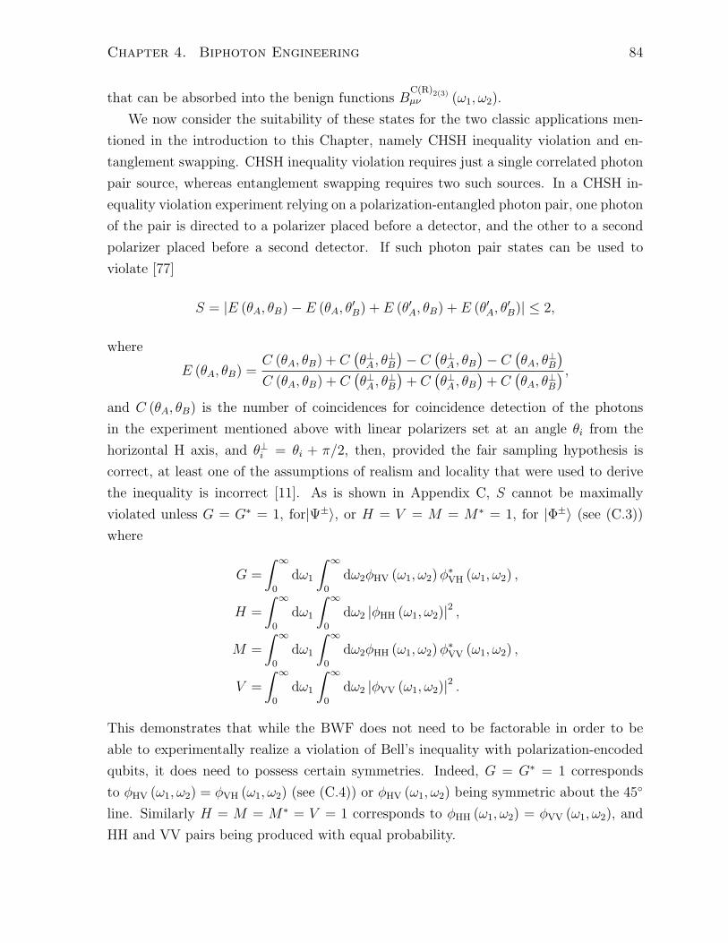
Chapter 4. Biphoton Engineering 84
that can be absorbed into the benign functions BC(R)2(3)µν (ω1, ω2).
We now consider the suitability of these states for the two classic applications men-
tioned in the introduction to this Chapter, namely CHSH inequality violation and en-
tanglement swapping. CHSH inequality violation requires just a single correlated photon
pair source, whereas entanglement swapping requires two such sources. In a CHSH in-
equality violation experiment relying on a polarization-entangled photon pair, one photon
of the pair is directed to a polarizer placed before a detector, and the other to a second
polarizer placed before a second detector. If such photon pair states can be used to
violate [77]
S = |E (θA, θB) − E (θA, θ′B) + E (θ′A, θB) + E (θ′A, θ
′B)| ≤ 2,
where
E (θA, θB) =C (θA, θB) + C
(θ⊥A , θ
⊥B
)− C
(θ⊥A , θB
)− C
(θA, θ
⊥B
)C (θA, θB) + C
(θ⊥A , θ
⊥B
)+ C
(θ⊥A , θB
)+ C
(θA, θ⊥B
) ,and C (θA, θB) is the number of coincidences for coincidence detection of the photons
in the experiment mentioned above with linear polarizers set at an angle θi from the
horizontal H axis, and θ⊥i = θi + π/2, then, provided the fair sampling hypothesis is
correct, at least one of the assumptions of realism and locality that were used to derive
the inequality is incorrect [11]. As is shown in Appendix C, S cannot be maximally
violated unless G = G∗ = 1, for|Ψ±⟩, or H = V = M = M∗ = 1, for |Φ±⟩ (see (C.3))
where
G =
∫ ∞
0
dω1
∫ ∞
0
dω2ϕHV (ω1, ω2)ϕ∗VH (ω1, ω2) ,
H =
∫ ∞
0
dω1
∫ ∞
0
dω2 |ϕHH (ω1, ω2)|2 ,
M =
∫ ∞
0
dω1
∫ ∞
0
dω2ϕHH (ω1, ω2)ϕ∗VV (ω1, ω2) ,
V =
∫ ∞
0
dω1
∫ ∞
0
dω2 |ϕVV (ω1, ω2)|2 .
This demonstrates that while the BWF does not need to be factorable in order to be
able to experimentally realize a violation of Bell’s inequality with polarization-encoded
qubits, it does need to possess certain symmetries. Indeed, G = G∗ = 1 corresponds
to ϕHV (ω1, ω2) = ϕVH (ω1, ω2) (see (C.4)) or ϕHV (ω1, ω2) being symmetric about the 45
line. Similarly H = M = M∗ = V = 1 corresponds to ϕHH (ω1, ω2) = ϕVV (ω1, ω2), and
HH and VV pairs being produced with equal probability.
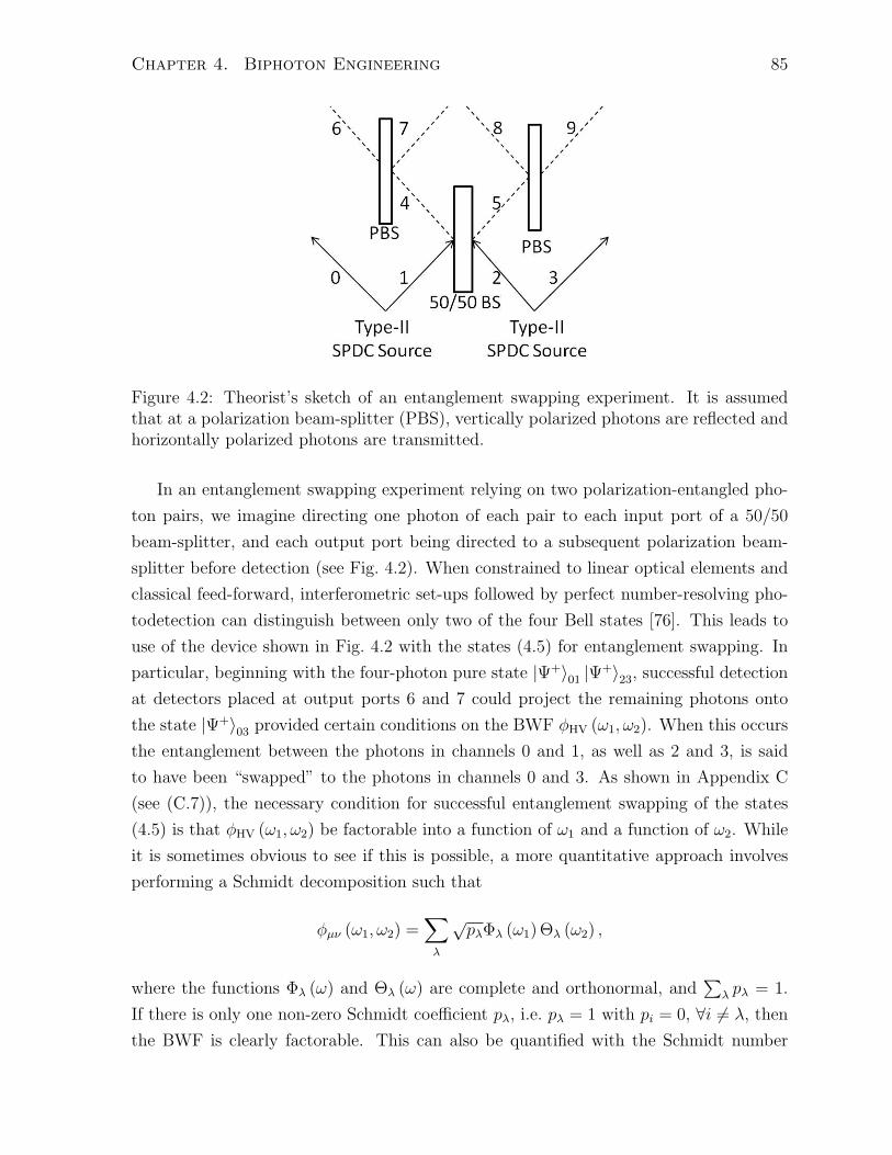
Chapter 4. Biphoton Engineering 85
Figure 4.2: Theorist’s sketch of an entanglement swapping experiment. It is assumedthat at a polarization beam-splitter (PBS), vertically polarized photons are reflected andhorizontally polarized photons are transmitted.
In an entanglement swapping experiment relying on two polarization-entangled pho-
ton pairs, we imagine directing one photon of each pair to each input port of a 50/50
beam-splitter, and each output port being directed to a subsequent polarization beam-
splitter before detection (see Fig. 4.2). When constrained to linear optical elements and
classical feed-forward, interferometric set-ups followed by perfect number-resolving pho-
todetection can distinguish between only two of the four Bell states [76]. This leads to
use of the device shown in Fig. 4.2 with the states (4.5) for entanglement swapping. In
particular, beginning with the four-photon pure state |Ψ+⟩01 |Ψ+⟩23, successful detection
at detectors placed at output ports 6 and 7 could project the remaining photons onto
the state |Ψ+⟩03 provided certain conditions on the BWF ϕHV (ω1, ω2). When this occurs
the entanglement between the photons in channels 0 and 1, as well as 2 and 3, is said
to have been “swapped” to the photons in channels 0 and 3. As shown in Appendix C
(see (C.7)), the necessary condition for successful entanglement swapping of the states
(4.5) is that ϕHV (ω1, ω2) be factorable into a function of ω1 and a function of ω2. While
it is sometimes obvious to see if this is possible, a more quantitative approach involves
performing a Schmidt decomposition such that
ϕµν (ω1, ω2) =∑λ
√pλΦλ (ω1) Θλ (ω2) ,
where the functions Φλ (ω) and Θλ (ω) are complete and orthonormal, and∑
λ pλ = 1.
If there is only one non-zero Schmidt coefficient pλ, i.e. pλ = 1 with pi = 0, ∀i = λ, then
the BWF is clearly factorable. This can also be quantified with the Schmidt number
Chapter 4. Biphoton Engineering 86
K = (∑
λ p2λ)
−1[63], which reaches a minimum of 1 when the BWF is factorable, and
is larger otherwise. We note that the more well-known version of the Schmidt number
as defined in e.g. Nielsen and Chuang [11] is simply the number of non-zero Schmidt
coefficients. However, as we are not interested in doing any calculations with the Schmidt
number but simply using it to characterize the frequency correlations in a given BWF,
we prefer Law and Eberly’s definition K [63]. Theirs appears more reasonable from a
physical point of view, for if there were 1000 Schmidt coefficients and 999 of them were
only as large as 10−5, Nielsen and Chuang’s definition would give a Schmidt number of
1000, whereas K ≈ 1.02. As mentioned in the introduction to this Chapter, approximate
methods of determining the Schmidt number K, and thus whether a BWF is factorable
and the photons from a given source suitable for, say, entanglement swapping, will be
presented in Section 4.4.
4.3 Shaping
For ease of comparing the shapes of the four biphoton probability densities introduced
above, we center all of them at the origin. Defining Ω1 = ω1 − ωµ, Ω2 = ω2 − ων ,
Ω = ω − ωP, with ωµ + ων = ωP for SPDC and ωµ + ων = 2ωP for SFWM, as well as
Taylor expanding dispersion relations to second order
km (ω) = km (ωm) + v−1m (ω − ωm) + Λm (ω − ωm)2 ,
we have
|ϕP (Ω)|2 =exp (−Ω2/∆2
ω)√2π∆ω
, (4.7)
with
∣∣θC2µν (Ω1,Ω2)
∣∣2 = sinc2[v−1µ Ω1 + v−1
ν Ω2 − v−1P (Ω1 + Ω2)
+ ΛµΩ21 + ΛνΩ2
2 − ΛP (Ω1 + Ω2)2]L/2 , (4.8)
∣∣θR2µν (Ω1,Ω2)
∣∣2 =[Ω2
µ + Ω21
]−1 [Ω2
ν + Ω22
]−1 [Ω2
P + (Ω1 + Ω2)2]−1
, (4.9)
for SPDC and
∣∣θC3µν (Ω1,Ω2)
∣∣2 =
∣∣∣∣∫ Ω1+Ω2
−ωP
dΩϕP (Ω)ϕP (Ω1 + Ω2 − Ω) sinc[v−1µ Ω1 + v−1
ν Ω2 − v−1P (Ω1 + Ω2)
+ ΛµΩ21 + ΛνΩ2
2 − ΛPΩ2 − ΛP (Ω1 + Ω2 − Ω)2]L/2
∣∣∣∣2 , (4.10)
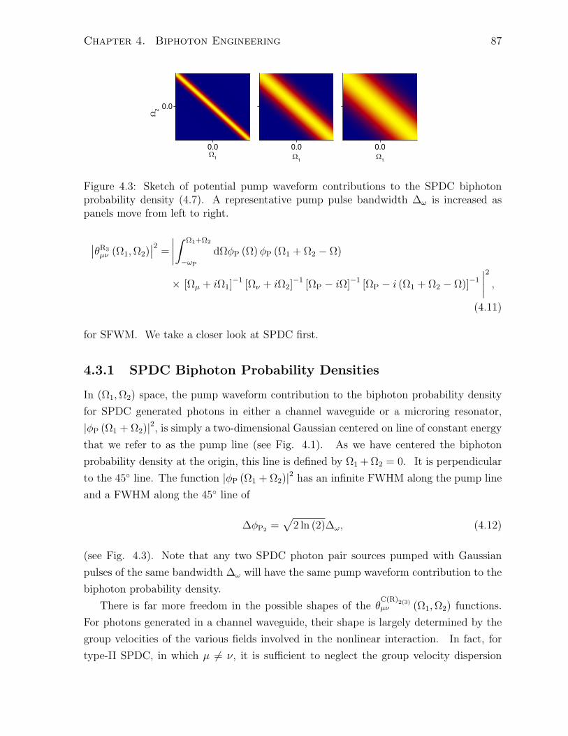
Chapter 4. Biphoton Engineering 87
0.0
0.021
0.01
0.01
Figure 4.3: Sketch of potential pump waveform contributions to the SPDC biphotonprobability density (4.7). A representative pump pulse bandwidth ∆ω is increased aspanels move from left to right.
∣∣θR3µν (Ω1,Ω2)
∣∣2 =
∣∣∣∣∫ Ω1+Ω2
−ωP
dΩϕP (Ω)ϕP (Ω1 + Ω2 − Ω)
× [Ωµ + iΩ1]−1 [Ων + iΩ2]
−1 [ΩP − iΩ]−1 [ΩP − i (Ω1 + Ω2 − Ω)]−1
∣∣∣∣2 ,(4.11)
for SFWM. We take a closer look at SPDC first.
4.3.1 SPDC Biphoton Probability Densities
In (Ω1,Ω2) space, the pump waveform contribution to the biphoton probability density
for SPDC generated photons in either a channel waveguide or a microring resonator,
|ϕP (Ω1 + Ω2)|2, is simply a two-dimensional Gaussian centered on line of constant energy
that we refer to as the pump line (see Fig. 4.1). As we have centered the biphoton
probability density at the origin, this line is defined by Ω1 + Ω2 = 0. It is perpendicular
to the 45 line. The function |ϕP (Ω1 + Ω2)|2 has an infinite FWHM along the pump line
and a FWHM along the 45 line of
∆ϕP2 =√
2 ln (2)∆ω, (4.12)
(see Fig. 4.3). Note that any two SPDC photon pair sources pumped with Gaussian
pulses of the same bandwidth ∆ω will have the same pump waveform contribution to the
biphoton probability density.
There is far more freedom in the possible shapes of the θC(R)2(3)µν (Ω1,Ω2) functions.
For photons generated in a channel waveguide, their shape is largely determined by the
group velocities of the various fields involved in the nonlinear interaction. In fact, for
type-II SPDC, in which µ = ν, it is sufficient to neglect the group velocity dispersion
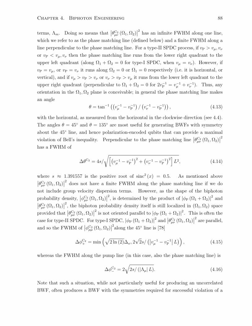
Chapter 4. Biphoton Engineering 88
terms, Λm. Doing so means that∣∣θC2
µν (Ω1,Ω2)∣∣2 has an infinite FWHM along one line,
which we refer to as the phase matching line (defined below) and a finite FWHM along a
line perpendicular to the phase matching line. For a type-II SPDC process, if vP > vµ, vν
or vP < vµ, vν then the phase matching line runs from the lower right quadrant to the
upper left quadrant (along Ω1 + Ω2 = 0 for type-I SPDC, when vµ = vν). However, if
vP = vµ, or vP = vν it runs along Ω2 = 0 or Ω1 = 0 respectively (i.e. it is horizontal, or
vertical), and if vµ > vP > vν or vν > vP > vµ it runs from the lower left quadrant to the
upper right quadrant (perpendicular to Ω1 + Ω2 = 0 for 2v−1P = v−1
µ + v−1ν ). Thus, any
orientation in the Ω1,Ω2 plane is conceivable; in general the phase matching line makes
an angle
θ = tan−1((v−1µ − v−1
P
)/(v−1ν − v−1
P
)), (4.13)
with the horizontal, as measured from the horizontal in the clockwise direction (see 4.4).
The angles θ = 45 and θ = 135 are most useful for generating BWFs with symmetry
about the 45 line, and hence polarization-encoded qubits that can provide a maximal
violation of Bell’s inequality. Perpendicular to the phase matching line∣∣θC2
µν (Ω1,Ω2)∣∣2
has a FWHM of
∆θC2 = 4s/
√[(v−1µ − v−1
P
)2+(v−1ν − v−1
P
)2]L2, (4.14)
where s ≈ 1.391557 is the positive root of sinc2 (x) = 0.5. As mentioned above∣∣θC2µν (Ω1,Ω2)
∣∣2 does not have a finite FWHM along the phase matching line if we do
not include group velocity dispersion terms. However, as the shape of the biphoton
probability density,∣∣ϕC2
µν (Ω1,Ω2)∣∣2, is determined by the product of |ϕP (Ω1 + Ω2)|2 and∣∣θC2
µν (Ω1,Ω2)∣∣2, the biphoton probability density itself is still localized in (Ω1,Ω2) space
provided that∣∣θC2
µν (Ω1,Ω2)∣∣2 is not oriented parallel to |ϕP (Ω1 + Ω2)|2. This is often the
case for type-II SPDC. For type-I SPDC, |ϕP (Ω1 + Ω2)|2 and∣∣θC2
µν (Ω1,Ω2)∣∣2 are parallel,
and so the FWHM of∣∣ϕC2
µµ (Ω1,Ω2)∣∣2along the 45 line is [78]
∆ϕC2+ = min
(√2 ln (2)∆ω, 2
√2s/
(∣∣v−1µ − v−1
P
∣∣L)) , (4.15)
whereas the FWHM along the pump line (in this case, also the phase matching line) is
∆ϕC2− = 2
√2s/ (|Λµ|L). (4.16)
Note that such a situation, while not particularly useful for producing an uncorrelated
BWF, often produces a BWF with the symmetries required for successful violation of a
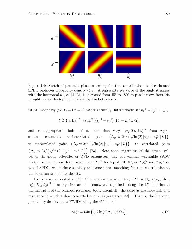
Chapter 4. Biphoton Engineering 89
0.0
2
0.0
0.0
2
1
0.01
0.01
Figure 4.4: Sketch of potential phase matching function contributions to the channelSPDC biphoton probability density (4.8). A representative value of the angle it makeswith the horizontal θ (see (4.13)) is increased from 45 to 180 as panels move from leftto right across the top row followed by the bottom row.
CHSH inequality (i.e. G = G∗ = 1) rather naturally. Interestingly, if 2v−1P = v−1
µ + v−1ν ,
∣∣θC2µν (Ω1,Ω2)
∣∣2 ≈ sinc2[(v−1µ − v−1
P
)(Ω1 − Ω2)L/2
],
and an appropriate choice of ∆ω can then vary∣∣ϕC2
µν (Ω1,Ω2)∣∣2 from repre-
senting essentially anti-correlated pairs(
∆ω ≪ 2s/(√
ln (2)∣∣v−1
µ − v−1P
∣∣L)),
to uncorrelated pairs(
∆ω ≈ 2s/(√
ln (2)∣∣v−1
µ − v−1P
∣∣L)), to correlated pairs(∆ω ≫ 2s/
(√ln (2)
∣∣v−1µ − v−1
P
∣∣L)) [73]. Note that, regardless of the actual val-
ues of the group velocities or GVD parameters, any two channel waveguide SPDC
photon pair sources with the same θ and ∆θC2 for type-II SPDC, or ∆ϕC2+ and ∆ϕC2
− for
type-I SPDC, will make essentially the same phase matching function contribution to
the biphoton probability density.
For photons generated via SPDC in a microring resonator, if ΩP ≈ Ωµ ≈ Ων , then∣∣θR2µν (Ω1,Ω2)
∣∣2 is nearly circular, but somewhat “squished” along the 45 line due to
the linewidth of the pumped resonance being essentially the same as the linewidth of a
resonance in which a downconverted photon is generated [33]. That is, the biphoton
probability density has a FWHM along the 45 line of
∆ϕR2+ = min
(√2 ln (2)∆ω,
√2ΩP
), (4.17)
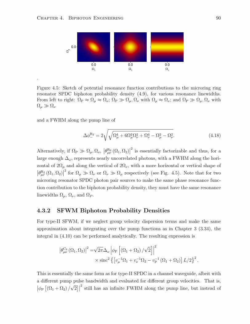
Chapter 4. Biphoton Engineering 90
0.0
0.0
21
0.01
0.01
.
Figure 4.5: Sketch of potential resonance function contributions to the microring ringresonator SPDC biphoton probability density (4.9), for various resonance linewidths.From left to right: ΩP ≈ Ωµ ≈ Ων ; ΩP ≫ Ωµ,Ων with Ωµ ≈ Ων ; and ΩP ≫ Ωµ,Ων withΩµ ≫ Ων
and a FWHM along the pump line of
∆ϕR2− = 2
√√Ω4
µ + 6Ω2µΩ2
ν + Ω4ν − Ω2
µ − Ω2ν . (4.18)
Alternatively, if ΩP ≫ Ωµ,Ων ,∣∣θR2
µν (Ω1,Ω2)∣∣2 is essentially factorizable and thus, for a
large enough ∆ω, represents nearly uncorrelated photons, with a FWHM along the hori-
zontal of 2Ωµ and along the vertical of 2Ων , with a more horizontal or vertical shape of∣∣θR2µν (Ω1,Ω2)
∣∣2 for Ωµ ≫ Ων or Ων ≫ Ωµ respectively (see Fig. 4.5). Note that for two
microring resonator SPDC photon pair sources to make the same phase resonance func-
tion contribution to the biphoton probability density, they must have the same resonance
linewidths Ωµ, Ων , and ΩP .
4.3.2 SFWM Biphoton Probability Densities
For type-II SFWM, if we neglect group velocity dispersion terms and make the same
approximation about integrating over the pump functions as in Chapter 3 (3.34), the
integral in (4.10) can be performed analytically. The resulting expression is
∣∣θC3µν (Ω1,Ω2)
∣∣2 =√
2π∆ω
∣∣∣ϕP
[(Ω1 + Ω2) /
√2]∣∣∣2
× sinc2[v−1µ Ω1 + v−1
ν Ω2 − v−1P (Ω1 + Ω2)
]L/2
2.
This is essentially the same form as for type-II SPDC in a channel waveguide, albeit with
a different pump pulse bandwidth and evaluated for different group velocities. That is,∣∣ϕP
[(Ω1 + Ω2) /
√2]∣∣2 still has an infinite FWHM along the pump line, but instead of
Chapter 4. Biphoton Engineering 91
a FWHM along the 45 line of√
2 ln (2)∆ω, as in (4.12), here the pump has a FWHM
along the 45 line of
∆ϕP3 = 2√
ln 2∆ω =√
2∆ϕP2 . (4.19)
Furthermore, as
∣∣θC2µν (Ω1,Ω2)
∣∣2 = sinc2[v−1µ Ω1 + v−1
ν Ω2 − v−1P (Ω1 + Ω2)
]L/2
,
when group velocity dispersion terms can be neglected, the sinc squared function in∣∣θC3µν (Ω1,Ω2)
∣∣2 has an infinite FWHM along the phase matching line, which is rotated
clockwise through an angle θ from the horizontal, as above (see (4.13)), and a FWHM in
the direction perpendicular to the phase matching line of ∆θC2 , also as above (see(4.14)).
Note that again we only make a connection between the forms of the SPDC and SFWM
functions - their arguments need not be the same.
When µ = ν instead, group velocity terms must be kept, and an analytic result
becomes possible only in the limit of a long pulse
∣∣θC3µµ (Ω1,Ω2)
∣∣2 ∝ ∣∣∣ϕP
[(Ω1 + Ω2) /
√2]∣∣∣2
× sinc2[(
v−1µ − v−1
P
)(Ω1 + Ω2)
+ (Λµ/2 − ΛP) (Ω1 + Ω2)2 + Λµ/2 (Ω1 − Ω2)
2]L/22=∣∣∣ϕP
[(Ω1 + Ω2) /
√2]∣∣∣2 ∣∣θC2
µµ (Ω1,Ω2)∣∣2
such that, as above, the FWHM of∣∣ϕC3
µµ (Ω1,Ω2)∣∣2 along the 45 line is
∆ϕC3+ = min
(2√
ln (2)∆ω, 2√
2s/(∣∣v−1
µ − v−1P
∣∣L)) ,and the FWHM along the pump line (in this case, also the phase matching line) is (4.16)
∆ϕC3− = ∆ϕC2
− = 2√
2s/ (|Λµ|L). (4.20)
Thus we see that it is mathematically possible to achieve identical biphoton probabil-
ity densities from channel resonator SPDC and SFWM pair sources, provided that the
relevant pump waveform contributions, group velocities and/or GVD parameters can be
made identical. In practice, however, it is likely that this is only achievable over a given
frequency range and not over the entire phase matching bandwidth. Furthermore, note
that while channel SFWM biphoton probability densities associated with shorter dura-
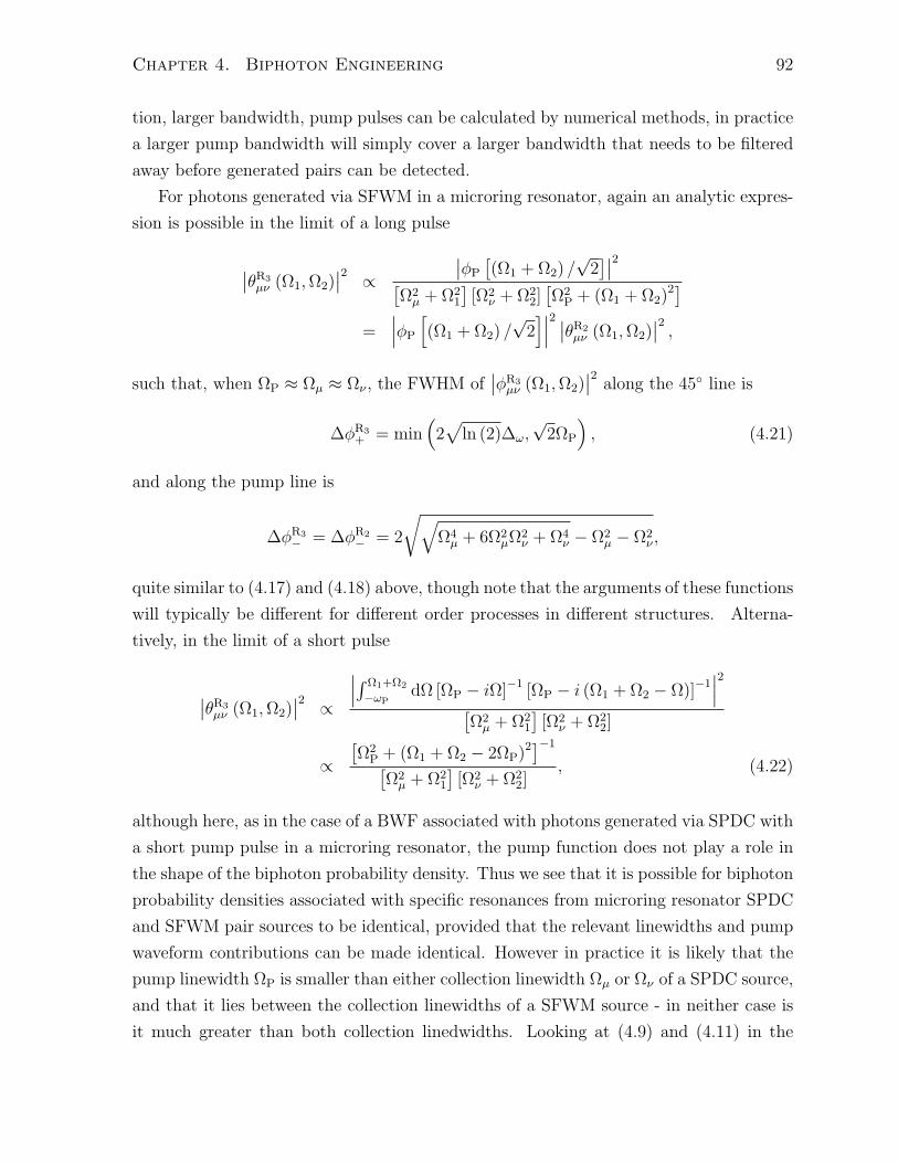
Chapter 4. Biphoton Engineering 92
tion, larger bandwidth, pump pulses can be calculated by numerical methods, in practice
a larger pump bandwidth will simply cover a larger bandwidth that needs to be filtered
away before generated pairs can be detected.
For photons generated via SFWM in a microring resonator, again an analytic expres-
sion is possible in the limit of a long pulse
∣∣θR3µν (Ω1,Ω2)
∣∣2 ∝∣∣ϕP
[(Ω1 + Ω2) /
√2]∣∣2[
Ω2µ + Ω2
1
][Ω2
ν + Ω22][Ω2
P + (Ω1 + Ω2)2]
=∣∣∣ϕP
[(Ω1 + Ω2) /
√2]∣∣∣2 ∣∣θR2
µν (Ω1,Ω2)∣∣2 ,
such that, when ΩP ≈ Ωµ ≈ Ων , the FWHM of∣∣ϕR3
µν (Ω1,Ω2)∣∣2 along the 45 line is
∆ϕR3+ = min
(2√
ln (2)∆ω,√
2ΩP
), (4.21)
and along the pump line is
∆ϕR3− = ∆ϕR2
− = 2
√√Ω4
µ + 6Ω2µΩ2
ν + Ω4ν − Ω2
µ − Ω2ν ,
quite similar to (4.17) and (4.18) above, though note that the arguments of these functions
will typically be different for different order processes in different structures. Alterna-
tively, in the limit of a short pulse
∣∣θR3µν (Ω1,Ω2)
∣∣2 ∝
∣∣∣∫ Ω1+Ω2
−ωPdΩ [ΩP − iΩ]−1 [ΩP − i (Ω1 + Ω2 − Ω)]−1
∣∣∣2[Ω2
µ + Ω21
][Ω2
ν + Ω22]
∝[Ω2
P + (Ω1 + Ω2 − 2ΩP)2]−1[
Ω2µ + Ω2
1
][Ω2
ν + Ω22]
, (4.22)
although here, as in the case of a BWF associated with photons generated via SPDC with
a short pump pulse in a microring resonator, the pump function does not play a role in
the shape of the biphoton probability density. Thus we see that it is possible for biphoton
probability densities associated with specific resonances from microring resonator SPDC
and SFWM pair sources to be identical, provided that the relevant linewidths and pump
waveform contributions can be made identical. However in practice it is likely that the
pump linewidth ΩP is smaller than either collection linewidth Ωµ or Ων of a SPDC source,
and that it lies between the collection linewidths of a SFWM source - in neither case is
it much greater than both collection linedwidths. Looking at (4.9) and (4.11) in the
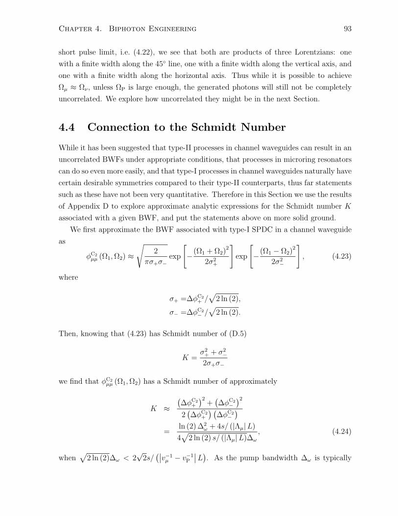
Chapter 4. Biphoton Engineering 93
short pulse limit, i.e. (4.22), we see that both are products of three Lorentzians: one
with a finite width along the 45 line, one with a finite width along the vertical axis, and
one with a finite width along the horizontal axis. Thus while it is possible to achieve
Ωµ ≈ Ων , unless ΩP is large enough, the generated photons will still not be completely
uncorrelated. We explore how uncorrelated they might be in the next Section.
4.4 Connection to the Schmidt Number
While it has been suggested that type-II processes in channel waveguides can result in an
uncorrelated BWFs under appropriate conditions, that processes in microring resonators
can do so even more easily, and that type-I processes in channel waveguides naturally have
certain desirable symmetries compared to their type-II counterparts, thus far statements
such as these have not been very quantitative. Therefore in this Section we use the results
of Appendix D to explore approximate analytic expressions for the Schmidt number K
associated with a given BWF, and put the statements above on more solid ground.
We first approximate the BWF associated with type-I SPDC in a channel waveguide
as
ϕC2µµ (Ω1,Ω2) ≈
√2
πσ+σ−exp
[−(Ω1 + Ω2)
2
2σ2+
]exp
[−(Ω1 − Ω2)
2
2σ2−
], (4.23)
where
σ+ =∆ϕC2+ /√
2 ln (2),
σ− =∆ϕC2− /√
2 ln (2).
Then, knowing that (4.23) has Schmidt number of (D.5)
K =σ2+ + σ2
−
2σ+σ−
we find that ϕC2µµ (Ω1,Ω2) has a Schmidt number of approximately
K ≈(∆ϕC2
+
)2+(∆ϕC2
−)2
2(∆ϕC2
+
) (∆ϕC2
−)
=ln (2) ∆2
ω + 4s/ (|Λµ|L)
4√
2 ln (2) s/ (|Λµ|L)∆ω
, (4.24)
when√
2 ln (2)∆ω < 2√
2s/(∣∣v−1
µ − v−1P
∣∣L). As the pump bandwidth ∆ω is typically
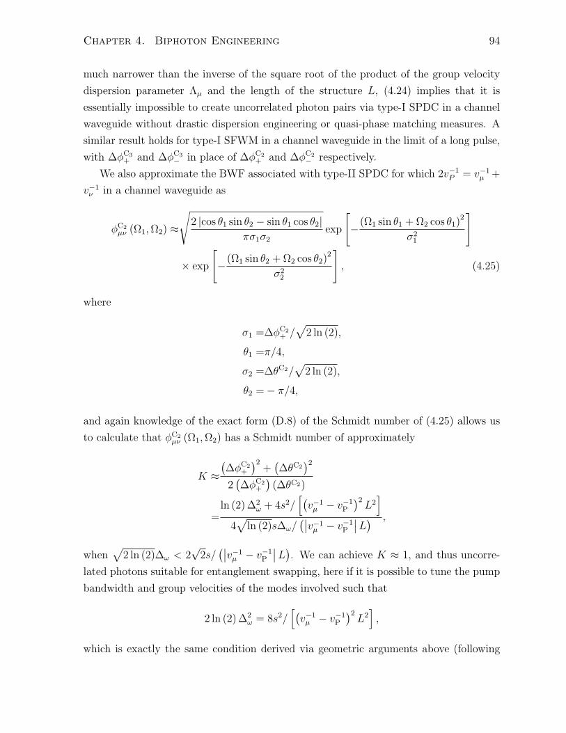
Chapter 4. Biphoton Engineering 94
much narrower than the inverse of the square root of the product of the group velocity
dispersion parameter Λµ and the length of the structure L, (4.24) implies that it is
essentially impossible to create uncorrelated photon pairs via type-I SPDC in a channel
waveguide without drastic dispersion engineering or quasi-phase matching measures. A
similar result holds for type-I SFWM in a channel waveguide in the limit of a long pulse,
with ∆ϕC3+ and ∆ϕC3
− in place of ∆ϕC2+ and ∆ϕC2
− respectively.
We also approximate the BWF associated with type-II SPDC for which 2v−1P = v−1
µ +
v−1ν in a channel waveguide as
ϕC2µν (Ω1,Ω2) ≈
√2 |cos θ1 sin θ2 − sin θ1 cos θ2|
πσ1σ2exp
[−(Ω1 sin θ1 + Ω2 cos θ1)
2
σ21
]
× exp
[−(Ω1 sin θ2 + Ω2 cos θ2)
2
σ22
], (4.25)
where
σ1 =∆ϕC2+ /√
2 ln (2),
θ1 =π/4,
σ2 =∆θC2/√
2 ln (2),
θ2 = − π/4,
and again knowledge of the exact form (D.8) of the Schmidt number of (4.25) allows us
to calculate that ϕC2µν (Ω1,Ω2) has a Schmidt number of approximately
K ≈(∆ϕC2
+
)2+(∆θC2
)22(∆ϕC2
+
)(∆θC2)
=ln (2) ∆2
ω + 4s2/[(v−1µ − v−1
P
)2L2]
4√
ln (2)s∆ω/(∣∣v−1
µ − v−1P
∣∣L) ,
when√
2 ln (2)∆ω < 2√
2s/(∣∣v−1
µ − v−1P
∣∣L). We can achieve K ≈ 1, and thus uncorre-
lated photons suitable for entanglement swapping, here if it is possible to tune the pump
bandwidth and group velocities of the modes involved such that
2 ln (2) ∆2ω = 8s2/
[(v−1µ − v−1
P
)2L2],
which is exactly the same condition derived via geometric arguments above (following
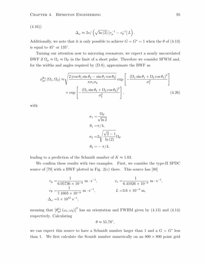
Chapter 4. Biphoton Engineering 95
(4.16))
∆ω ≈ 2s/(√
ln (2)∣∣v−1
µ − v−1P
∣∣L) .Additionally, we note that it is only possible to achieve G = G∗ = 1 when the θ of (4.13)
is equal to 45 or 135.
Turning our attention now to microring resonators, we expect a nearly uncorrelated
BWF if Ωµ ≈ Ων ≈ ΩP in the limit of a short pulse. Therefore we consider SFWM and,
for the widths and angles required by (D.8), approximate the BWF as
ϕR3µν (Ω1,Ω2) ≈
√2 |cos θ1 sin θ2 − sin θ1 cos θ2|
πσ1σ2exp
[−(Ω1 sin θ1 + Ω2 cos θ1)
2
σ21
]
× exp
[−(Ω1 sin θ2 + Ω2 cos θ2)
2
σ22
], (4.26)
with
σ1 =ΩP√ln 2
θ1 =π/4,
σ2 =2
√√2 − 1
ln (2)ΩP
θ2 = − π/4,
leading to a prediction of the Schmidt number of K ≈ 1.03.
We confirm these results with two examples. First, we consider the type-II SPDC
source of [79] with a BWF plotted in Fig. 2(c) there. This source has [80]
vµ =1
6.05736 × 10⁻⁹m · s−1, vν =
1
6.41026 × 10⁻⁹m · s−1,
vP =1
7.1603 × 10⁻⁹m · s−1, L =3.6 × 10⁻³ m,
∆ω =5 × 10¹² s−1,
meaning that∣∣θC2
µν (ω1, ω2)∣∣2 has an orientation and FWHM given by (4.13) and (4.14)
respectively. Calculating
θ ≈ 55.78,
we can expect this source to have a Schmidt number larger than 1 and a G = G∗ less
than 1. We first calculate the Scmidt number numerically on an 800 × 800 point grid
Chapter 4. Biphoton Engineering 96
spanning from −1 × 10¹⁴ s−1 to 1 × 10¹⁴ s−1 along both axes, and find K = 18.5. This
corresponds to an entropy of entanglement
E = −∑λ
pλ log2 pλ,
of E ≈ 4.55 which is quite close to the value published in [79] of E = 4.6. Calculating K
instead using the analytic result (D.8) for the Gaussian approximation (4.25), we have
σ1 =∆ω
≈5 × 10¹² s−1
θ1 =π/4,
σ2 =2√
2s√ln 2
[(v−1µ − v−1
P
)2+(v−1ν − v−1
P
)2]L2
≈9.8455 × 10¹¹ s−1,
θ2 = tan−1
(v−1µ − v−1
P
v−1ν − v−1
P
)≈ 55.78,
and thus find K ≈ 13.2. This demonstrates that while the double Gaussian approxi-
mation of Appendix D is useful for obtaining an approximation to the Schmidt number,
it cannot capture the oscillations of the squared sinc function and therefore underesti-
mates the true Schmidt number. Indeed, when the double-Gaussian form of the BWF
is calculated numerically, we also find K ≈ 13.2. Both values suggest that this source
is not suitable as a source for an entanglement swapping protocol. This source also
has G = G∗ ≈ 0.1, and so fringe visibility will be reduced in correlated polarization
measurements.
Second, we consider the SFWM ring resonator source of [33] with a biphoton wave
function plotted in Fig. 2(b) there. This source has
∆ω =
√2 ln 2
vT, v = 1.71 × 10⁸ m · s−1, T = 5 ns,
Ωµ ≈Ων ≈ ΩP = 2π (0.74 GHz) ,
meaning that it has a biphoton probability density that looks like (4.22), with widths
along the 45 line and pump line of (4.21) and (4.18) respectively. We thus expect this
Chapter 4. Biphoton Engineering 97
source to have K ≈ 1.03. While not exact, this value is also close to the published
(numerically calculated) value of K = 1.09. Again, the double Gaussian approximation
has slightly simplified things and therefore caused an underestimation of the true Schmidt
number. Nevertheless, the Schmidt number is nearly unity, demonstrating that this
source is much more suitable than the other for creating photon pairs to be used for
entanglement swapping.
4.5 Discussion
In this Chapter I have examined the biphoton probability densities associated with pho-
ton pairs generated via SPDC or SFWM in either a channel waveguide or microring
resonator side-coupled to a channel waveguide under idealized conditions. In Section 4.1
they were written in a general form that made it easy to see the terms most responsible for
their shape. While many terms are rather benign, the pump function and phase match-
ing sinc function in a channel waveguide, and pump function and Lorentzian linewidth
functions in a microring resonator have a great deal of influence over the shape of the
biphoton probability density. In Section 4.2 I considered two potential uses of photon
pairs, violation of Bell’s inequality, which involves just a single source and destroys both
photons, and entanglement swapping, which involves two sources and uses two photons
to fix the state of the other two. While the polarization-entangled qubits used in these
applications are often thought of as being single-mode, a more general theory using the
states introduced in Section 4.1 suggests that they are frequency correlated. These cor-
relations are characterized by a biphoton probability density that, as was shown here,
must possess certain properties in order for the application to be successful. It must have
certain symmetries to maximally violate Bell’s inequality, and must be factorable for per-
fect entanglement swapping. In Section 4.3 parameters that govern these properties are
identified, and in Section 4.4 analytic expressions for the Schmidt number are presented
and put to the test. In a channel waveguide, there are many ways to use dispersion
engineering to achieve the group velocities necessary to allow control of the correlations
of the generated photons by tuning only the spectral width of the pump. In a microring
resonator, provided resonances can be found that satisfy both energy conservation and
phase matching, this control essentially happens for free. However, to get truly uncor-
related photons, and not a Schmidt number simply “near” 1, one needs to engineer the
FWHMs of the resonance linewidths associated with the fields involved in the photon
generation process. In practice, it may be difficult to achieve a pump resonance linewidth
that is much larger than either of the other two resonance linewidths, ΩP ≫ Ωµ,Ων , as

Chapter 4. Biphoton Engineering 98
resonance linewidths are generally going to be narrower at higher frequencies due to the
evanescent field outside the waveguide dropping off more quickly at higher frequencies.
Still, in a device in which the pump and generated photons are in different modes, it may
be possible to work around this issue.
Chapter 5
Powers at Which Nonlinear
Processes Become Important
Up until now calculations have largely ignored nonlinear effects other than the photon
pair generation process under consideration. This makes for clean and intuitive expres-
sions, but leaves much to worry about. Two-photon absorption (TPA) and associated
free-carrier absorption (FCA) could cause generated photons to become lost, self-phase
modulation (SPM) of the pump and cross-phase modulation (XPM) of the generated
photons could cause the optimal pump and collection frequencies to shift, multiple pairs
could be produced simultaneously instead of a single pair, and dispersion of the pump
pulse could become important if shorter and shorter pulses are used to increase the peak
pump power. Yet even without taking any of these effects into account, the scaling rela-
tionships developed in Chapter 3 do a decent job of predicting the photon pair generation
efficiency of a device [81, 18]. To explain this, in this chapter I clarify the relationship be-
tween the various nonlinear processes mentioned above in photon pair sources made of a
material with only a third-order nonlinearity χ3, and demonstrate that if one works with
pump powers low enough to suppress multi-pair generation, one is often automatically
constraining the strength of many other nonlinear processes as well.
In Section 5.1 we derive expressions for when multi-pair production becomes relevant
for a SFWM process both in a channel waveguide and a microring resonator. Written as
inequalities, they allow for easy comparison with known conditions for the pump powers
at which other nonlinear processes become relevant. In Section 5.2 these inequalities are
put to the test for devices in the literature, taking a channel waveguide and a microring
resonator as specific examples, and a discussion of these results follows in Section 5.3.
Linear (scattering) loss is addressed in the following Chapter.
99
Chapter 5. Powers at Which Nonlinear Processes Become Important100
5.1 A Series of Inequalities
As discussed in Chapter 2 following Eq. (3.12) for a state of generated photons of the
form
|ψgen⟩ = exp(βC†
II − H.c.)|vac⟩ ,
exiting the right R channel of a given device, where
C†II =
1√2
∫ ∞
0
dω1
∫ ∞
0
dω2ϕ (ω1, ω2) b†Rω1
b†Rω2,
when |β| ≪ 1
|ψgen⟩ ≈ |vac⟩ + βC†II |vac⟩ ,
and |β|2 can be thought of as the average number of generated photon pairs per pump
pulse. Dividing (3.40) and (3.57) by T/ (~ωP) where T is the duration of the pump
pulse, in the long-pulse limit we find that the total pair production probability is
NC3,idealpairs =
∣∣βC3∣∣2 =
2
3(γPPL)2
√T 2
2π |β2 (ωP)|L, (5.1)
in a channel waveguide and
NR3,idealpairs =
∣∣βR3∣∣2 =
vPL
2(γPP)2 |FP (ωP)|6 T, (5.2)
in a microring resonator side-coupled to a channel waveguide, just as in Appendix B.
Here γ = 3χ3ωP/ (4ε0v2n4A) is the usual nonlinear parameter [43] with A an effective
area (3.33), the GVD parameter β2 = d2k/dω2∣∣ωP
, PP = ~ωPNP/T is the average pump
power, |FP (ωP)| is a resonant field enhancement factor (3.46), and L is the length of the
device. Furthermore, it has been assumed that the channel waveguide is pumped at its
phase-matching frequency, and the ring resonator at a resonance frequency with adjacent
generated photon collection resonances that are phase-matched and conserve energy (i.e.
pumped near the zero dispersion wavelength). While TPA, FCA, SPM, and XPM have
been neglected in these calculations, we note that they represent the maximum possible
number of generated photon pairs per pump pulse, i.e. for a phase matched process the
inclusion of additional nonlinear effects would only lead to a lower number of generated
photon pairs, and so we refer to (5.1) and (5.2) as the ideal number of generated photon
pairs in each type of structure.
Chapter 5. Powers at Which Nonlinear Processes Become Important101
5.1.1 Pump Dispersion
For a channel waveguide, the long-pulse limit corresponds to the pump pulse bandwidth
∆P ≈ 4a/T , where a ≈ 1.8955 is the positive root of sinc (x) = 0.5 being smaller than the
phase-matching bandwidth ∆M = 4√a/ [|β2 (ωP)|L] whereas for a microring resonator
it corresponds to the pump pulse bandwidth being smaller than a resonance linewidth
∆R = ωP/Q where Q is the quality factor of the ring. Note that we have assumed a
pump pulse of the form
ϕP (ω) =
√T
2πsinc
((ω − ωP)
T
2
),
for these approximations, as in Appendix B, and that ∆M, with β2 (ωP) = 2Λµ, is closely
related to ∆C3− (4.20), as the former is a width of the BWF and the latter a width of
the biphoton probability density. The long-pulse limit ensures efficient photon pair
generation, as no pump bandwidth is wasted outside the phase-matching bandwidth or
resonance linewidth. Also, for systems in which ∆R ≪ ∆M, the long-pulse limit ensures
∆P ≪ ∆M
4a
T≪ 4
√a
|β2 (ωP)|L
L ≪ LD
a, (5.3)
where LD = T 2/ |β2| is the usual dispersion length [43]. Thus we see that if the pump
pulse is long enough to ensure that photons are generated efficiently [28], dispersion of
its waveform may be neglected during propagation through the device.
5.1.2 Self- and Cross-Phase Modulation
With pump pulse bandwidth concerns dispensed with, we now turn to considerations
regarding the pump pulse power. Introducing the nonlinear length LNL = (γPP)−1 [43],
we can rewrite (5.1) as
NC3,idealpairs =
2
3
(L
LNL
)2√
LD
2πL,
Then, if one demands that
NC3,idealpairs ≪ 1, (5.4)
because we have L ≪ LD (5.3), in order for the average number of generated pairs per
pump pulse in a channel waveguide to remain much less than one, and thus the average
Chapter 5. Powers at Which Nonlinear Processes Become Important102
probability of 4-photon generation much much less than one, we see that, qualitatively,
we must demand L ≪ LNL. We note that this is the condition required for one to
be able to neglect self- and cross-phase modulation effects. Thus simply by working
with pump pulses long enough and weak enough to ensure efficient pair generation per
pump pulse without any multi-pair generation, one also ensures that said pulses do not
undergo significant dispersion, undergo significant SPM, or affect significant XPM as
they propagate through the nonlinear device. Being a bit more precise we find that
(5.4) in fact demands
L≪(
9πL4NL
2LD
)1/3
, (5.5)
or
PP ≪(
9πL
2LD
)1/4
(γL)−1 . (5.6)
In the true CW limit, these become (see (B.7))
L≪(
9π
64s
)1/4
LNL, (5.7)
and
PP ≪(
9π
64s
)1/4
(γL)−1 , (5.8)
where s ≈ 1.3916 is the positive root of sinc2 (x) = 0.5.
The equations are similar for the ring resonator. We first rewrite (5.2) as
NR3,idealpairs =
1
2
(L
LNL
)2√
|β2|LDv2PL2
|FP (ωP)|6 ,
and, because L≪ LD demanding that
NR3,idealpairs ≪ 1, (5.9)
also qualitatively requires L ≪ LNL. However, being more careful, we find that (5.9) in
fact requires
L≪(
4L4NL
|β2|LDv2P
)1/2
|FP (ωP)|−6 , (5.10)
or
PP ≪(
4L2
|β2|LDv2P
)1/4
(γL)−1 |FP (ωP)|−3 . (5.11)
Chapter 5. Powers at Which Nonlinear Processes Become Important103
In the true CW limit (see (B.9)) these become
L≪
(√2 − 1
16s2
)1/4
LNL |FP (ωP)|−7/2 , (5.12)
and
PP ≪
(√2 − 1
16s2
)1/4
(γL)−1 |FP (ωP)|−7/2 . (5.13)
5.1.3 Two-Photon and Free-Carrier Absorption
We also consider FCA and TPA. Looking at Eq. (1) of [82], and based on the grounds
that self- and cross-phase modulation can be neglected for PP ≪ (γ L)−1, two-photon
absorption can be neglected in a channel waveguide provided
PP ≪ 2AβTPAL
, (5.14)
where βTPA is the TPA coefficient [82]. If we are working in the limit L ≪ LNL then if
one can show that
LNL . 2AβTPAPP
, (5.15)
or, written another way, thatβTPA
2A. γ,
then (5.14) is assuredly satisfied and two-photon absorption can safely be neglected.
Similarly, free-carrier absorption can be neglected in a channel waveguide provided
[83]
PP ≪ 3~ωPAσT
, (5.16)
where σ is the free-carrier absorption coefficient [83]. Again, given L ≪ LNL, if one is
able to show thatTσ
3~ωPAγ. L,
orTσ
3~ωPAL. γ,
then (5.16) is guaranteed to be satisfied. In the CW limit, from Eq. (2) of [83] (or Eq.
Chapter 5. Powers at Which Nonlinear Processes Become Important104
(2) of [82]), the free carrier density will reach steady-state at
βTPAP2Pτc
2~ωTA2,
where τc is the free-carrier lifetime, and so again referring to Eq. (1) of [82], we expect
FCA to be negligible in a CW experiment in a channel waveguide if
βTPAP2Pτc
2~ωPA2
σ
2L≪ 1,
or
PP ≪(
4~ωPA2
βTPAτcσL
)1/2
. (5.17)
Thus, knowing L≪ LNL, if one is able to show that(βTPAτcσ
4~ωPA2L
)1/2
. γ,
then (5.17) is guaranteed to be satisfied.
For pulsed SFWM in a channel waveguide, for instance, we see that if the photon
pair source is such that (9πL
2LD
)1/4βTPA
2A. γ,
and (9πL
2LD
)1/4Tσ
3~ωPAL. γ,
then by working in the long-pulse limit and keeping the pump power low enough to
suppress multi-pair production (5.6) one automatically also avoids pump pulse dispersion,
SPM, XPM, TPA, and FCA.
Note that if considering these processes in a microring resonator instead of a channel
waveguide, the pump powers at which TPA and FCA become relevant (the right hand
sides of (5.14), (5.16), and (5.17)) will be reduced by a factor of |FP (ωP)|2. Also, rather
than simply taking L ≪ LNL, a more precise calculation would involve substituting one
of (5.5), (5.7), (5.10), or (5.12), (5.6), (5.8), (5.11), or (5.13) for L or PP as appropriate..
Chapter 5. Powers at Which Nonlinear Processes Become Important105
5.2 A First Check
In this section we look at SFWM experiments in a silicon microring resonator [18] as well
as a silicon slow light photonic crystal [81]. The photon generation experiment in the
ring used a CW laser while the photonic crystal experiment used a pulsed laser with a
duration of T = 14 ps, both centered near λP = 1550 nm. In silicon, it is known that
n2 = 5 × 10⁻¹⁸ m2·W−1, βTPA = 1 × 10⁻¹¹ m·W−1, σ = 1.45 × 10⁻²¹ m2 [82], and τc = 1
ns [83]. The slow light structure has a length of 96 µm, while the microring resonator
has radius of 5 µm. In addition, the slow light structure has a nonlinear parameter
of γ × S2 ≈ 4000 m−1·W−1 while the ring has γ ≈ 190 m−1·W−1, where S ≈ 10 is a
slow-down factor [82]. Furthermore, the GVD parameter in the slow light structure is
β2 (ωP) = 1.3 ns2km−1, and the enhancement factor in the ring is |FP (ωP )|2 ≈ 390.
Knowing γ = 2πn2/ (λPA) means that in the ring A ≈ 0.11 µm2 in the ring and
A ≈ 0.51 µm2 in the slow-light structure. Thus, in the ring(√2 − 1
16s2
)1/4
|FP (ωP)|−3/2 βTPA
2A≈ 1.8 × 10⁻¹ m−1 · W−1,
and (√2 − 1
16s2
)1/4
|FP (ωP)|−3/2
(βTPAτcσ
4~ωPA2L
)1/2
≈ 3.1 × 10⁵ m−1 · W−1,
whereas in the photonic crystal
(9πL
2LD
) 14 βTPA × S2
2A≈ 3.0 × 10² m−1 · W−1,
and (9πL
2LD
) 14 Tσ × S
3~ωPAL≈ 3.3 × 10³ m−1 · W−1,
It is clear that in the photonic crystal, multi-pair production will occur for lower pump
powers than TPA, or FCA. In the ring, we still need to check if FCA will occur for
lower pump powers than other processes. More specifically, multi pair-production will
become an issue in the slow light structure unless (5.6) PP ≪ 0.80 W, FCA unless
(5.16) PP ≪ 0.96 W, SPM and XPM unless PP ≪[(γL)−1 =
]2.6 W, and TPA unless
(5.14) PP ≪ 10.6 W. In the ring resonator the hierarchy is much the same, multi-
pair production will become an issue unless (5.13) PP ≪ 1.7 mW, FCA unless (5.17)
PP ≪ 9.2 mW, SPM and XPM unless PP ≪[(γL |FP (ωP)|2
)−1=]
0.34 W, and TPA
unless PP ≪ 1.7 W. Perhaps not surprisingly, in the ring experiment, pump powers did
Chapter 5. Powers at Which Nonlinear Processes Become Important106
not go much higher than 1 mW, whereas in the slow-light structure experiment they were
kept under 0.7 W. This ensured that the pump powers were always under the lowest,
namely the multi-pair production power, inequality, and therefore allowed a theory that
did not take SPM, XPM, FCA, nor TPA into account to still make accurate predictions.
5.3 Discussion
In many photon pair generation experiments with integrated devices, one may worry
about the strength of nonlinear processes other than the one responsible for the generation
of photon pairs. In Section 5.1 of this Chapter, I have presented a number of equations
that suggest that, for an appropriately designed source, many of these processes need not
become important if one works with powers low enough to suppress multi-pair production.
These equations were confirmed by looking at the parameters associated with two photon
pair sources in the literature in Section 5.2. In both experiments, pump powers were
indeed kept below powers at which multi-pair production would become significant, with
powers at which XPM, SPM, FCA, or TPA would become significant all being higher.
Chapter 6
Loss
In this chapter I consider the effects of scattering loss on a given state of generated
photons. This certainly does not solve the problem of how to best account for photon
loss and generation simultaneously within the same medium, but is an important first
step that serves to demonstrate that there is nothing pathological about such loss when
introduced within a particular model.
To include loss in the kinds of systems introduced in Chapter 2, one can imagine
connecting the channel modes to systems of statistically independent reservoirs at tem-
perature T . This phenomenological model allows for light to couple out of the guided
waveguide modes to unguided modes, and the temperature of the reservoirs is eventually
taken to be 0 so that no light can ever scatter back into the waveguide modes. We note
that this assumption, which is quite reasonable here as room temperature blackbody
radiation at the frequencies of interest is negligible, greatly simplifies the calculation of
how a given state of generated photons decays.
Indeed from knowledge of how a coherent state decays when coupled to a zero-
temperature reservoir, one could perhaps try to include scattering loss “by hand” for
a given state of generated photons with a decaying exponential term that is fit with
data extracted from a classical experiment. However it is not entirely clear whether a
two-photon state should decay according to the same exponential term, or perhaps the
same exponential term squared, or how the single photon probability of a density oper-
ator that originally represented a two-photon state grows and then falls, not to mention
how a squeezed state behaves. Thus, loss is introduced here within the general Hamil-
tonian formalism of Chapter 2, preserving the necessary canonical equal-time bosonic
commutation relations as the system evolves, with a view to considering photon loss and
generation simultaneously. This approach enables the evolution of all of the pieces of a
given state of generated photons, expressed as a density operator, to be understood.
107
Chapter 6. Loss 108
The full Hamiltonian is now
H = HL +HNL +HR +HI,
where
HR =∑
n,I∈σn
∫dkdµ~ΩnIµkB
†nIµkBnIµk,
HI =∑
n,I∈σn
∫dkdµ~
(cnIµkb
†nIkBnIµk + c∗nIµkB
†nIµkbnIk
), (6.1)
with [bnIk, b
†n′I′k′
]=δnn′δII′δ (k − k′) ,[
BnIµk, B†n′I′µ′k′
]=δnn′δII′δ (µ− µ′) δ (k − k′) , (6.2)
and all other commutators zero; the µ describes the magnitude of the reservoir wavevec-
tors in directions transverse to the propagation direction of the guided waveguide mode.
From here, one could one could derive an expression for the evolution of the reduced
density operator for an asymptotic-in state composed of waveguide operators. Written
as a differential equation, this is known as the Master Equation, and can be put into
Lindblad form [84]. Alternatively, one could work with the Glauber-Sudarshan P func-
tion representation for the density operator [85, 86] and arrive at a Fokker-Planck type
equation [87, 88]. However, we find that the approach that most clearly captures the
physics and appears to lend itself to integration with the formalism introduced in Chap-
ter 2 is a quantum Langevin formalism in which equations of motion are derived for
waveguide operators in terms of “fluctuating” reservoir operators, which are later traced
out of the appropriate density operator. In what follows, we consider loss in the absence
of any nonlinearity and how it affects different “already generated” states. In Section 6.1
we introduce the general formalism, deriving expressions for the evolution of waveguide
operators, and in Section 6.2 we apply the formalism to a coherent state, a two-photon
state, and a squeezed vacuum state, before discussing these results in Section 6.3.
Chapter 6. Loss 109
6.1 Quantum Langevin Formalism
The Heisenberg equations of motion for the b†nIk (t) and B†nIµk (t) are (recall (2.41))
db†nIk (t)
dt= − i
~
[b†nIk (t) , HL +HR +HI
]= iωnIkb
†nIk (t) + i
∫dµc∗nIµkB
†nIµk (t) ,
dB†nIµk (t)
dt= − i
~
[B†
nIµk (t) , HL +HR +HI
]= iΩnIµkB
†nIµk (t) + icnIµkb
†nIk (t) , (6.3)
the second of which can be solved immediately
B†nIµk (t) = i
∫ t
t0
b†nIk (τ) cnIµkeiΩnIµk(t−τ)dτ +B†
nIµkeiΩnIµk(t−t0), (6.4)
where the lack of a time variable associated with the reservoir operator indicates that it
is a Schrodinger operator. Substituting (6.4) in the first of (6.3), we find
db†nIk (t)
dt=iωnIkb
†nIk (t)
+ i
∫dµc∗nIµk
(i
∫ t
t0
b†nIk (τ) cnIµkeiΩnIµk(t−τ)dτ +B†
nIµkeiΩnIµk(t−t0)
)=iωnIkb
†nIk (t)
−∫
dµ
(∫ t
t0
b†nIk (τ) |cnIµk|2 eiΩnIµk(t−τ)dτ + iB†nIµkc
∗nIµke
iΩnIµk(t−t0)
).
To evaluate the first integral, we note that the guided modes will only interact strongly
with reservoir modes that approximately conserve energy and momentum. If scattering
losses are small, we expect that when a guided mode is scattered out of the waveguide
it will keep essentially the same value of k and µ (µ = 0). Thus, we expect only a very
small range of µ values, centered about µ = 0, to be relevant to the problem. With this
in mind, we approximate |cnIµk|2 as constant over the µ of interest(|cnIµk|2
)µ=0
≡ cnIk
such that∫dµ
∫ t
t0
a†nIk (τ) |cnIµk|2 eiΩnIµk(t−τ)dτ = cnIk
∫dµ
∫ t
t0
a†nIk (τ) eiΩnIµk(t−τ)dτ.
Further, we write
dµ =dµ
dΩnIµk
dΩnIµk,
also approximating dµdΩnIµk
as constant,(
dµdΩnIµk
)µ=0
≡ 1v′nIk
, over the µ of interest, and
Chapter 6. Loss 110
arrive at a quantum mechanical Langevin equation
db†nIk (t)
dt=iωnIkb
†nIk (t) − cnIk
v′nIk
∫dΩnIµk
∫ t
t0
b†nIk (τ) eiΩnIµk(t−τ)dτ
− i
∫dµB†
nIµkc∗nIµke
iΩnIµk(t−t0)
= (iωnIk − βnIk) b†nIk (t) − F †nIk (t) , (6.5)
where we have defined the loss parameter
βnIk ≡ πcnIk/v′nIk, (6.6)
and the fluctuation term
F †nIk (t) ≡ i
∫dµB†
nIµkc∗nIµke
iΩnIµk(t−t0).
Although an exponential decay of b†nIk (t) is implied by (6.5) even without the fluctu-
ation term, the fluctuation term’s presence is necessary to ensure that the equal-time
commutation relations of b†nIk (t) do not vary with time, a property that will be verified
below. While it is possible, in principle, to determine the cnIk and thus the βnIk from first
principles, an ad hoc approach would be to determine the βnIk directly from the results
of classical experiments. Indeed βnIk is the object, not cnIk, that appears in equations
describing how a given state of generated photons decays.
The Langevin equation (6.5) has solution
b†nIk (t) = Λ†nIk (t) + Γ†
nIk (t) ,
where, setting t0 = 0 for convenience, we have defined
Γ†nIk (t) ≡−
∫ t
0
F †nIk (τ) e(iωnIk−βnIk)(t−τ)dτ
Λ†nIk (t) ≡b†nIke
(iωnIk−βnIk)t,
Chapter 6. Loss 111
with commutation relations (recall (6.2) and (6.6))[FnIk (t) , F †
n′I′k′ (t′)]
=2βnIkδnn′δII′δ (t− t′) δ (k − k′) ,[ΛnIk (t) ,Λ†
n′I′k′ (t)]
=e−2βnIktδnn′δII′δ (k − k′) ,[ΓnIk (t) ,Γ†
n′I′k′ (t)]
=(1 − e−2βnIkt
)δnn′δII′δ (k − k′) ,[
Λ†nIk (t) ,Γ†
n′I′k′ (t)]
=0. (6.7)
Note that, as required, the equal-time commutation relation for b†nIk (t) is the same as
that for b†nIk[bnIk (t) , b†n′I′k′ (t)
]=e−2βnIktδnn′δII′δ (k − k′) +
(1 − e−2βnIkt
)δnn′δII′δ (k − k′)
=δnn′δII′δ (k − k′) .
6.2 Propagation Examples
We describe the evolution of the state incident on the lossy region with a reduced den-
sity operator, found by forming the linear system density operator and tracing over the
reservoir oscillators
ρred (t) = TrR(ρtot (t)
)= TrR (|ψ (t)⟩ ⟨ψ (t)|) ,
at temperature T = 0. In all of the following examples we consider a single mode state
propagating in a single channel, and so drop the unnecessary labels n and I.
6.2.1 Coherent State
As a first example, we consider a coherent state
|ψ⟩coh = |z⟩ = ezA†0−H.c. |vac⟩ , (6.8)
where z is a complex number,
A†0 =
∫dkϕ0 (k) b†k,
Chapter 6. Loss 112
and ∫dk |ϕ0 (k)|2 = 1.
In writing |vac⟩ we have implicitly assumed that it consists of both a system part and
a reservoir part |vac⟩ = |vac⟩S ⊗ |vac⟩R, and while the eventual trace will be taken over
only the reservoir part, leaving the system part behind, we will still write just |vac⟩ for
simplicity of notation. The temporal evolution of this state can be expressed as a product
of system and reservoir states
|ψ (t)⟩coh =ez∫dkϕ0(k)b
†k(t)−H.c. |vac⟩
=ez∫dkϕ0(k)[Λ†
k(t)+Γ†k(t)]−H.c. |vac⟩
=ez∫dkϕ0(k)Λ
†k(t)−H.c. |vac⟩ ez
∫dkϕ0(k)Γ
†k(t)−H.c. |vac⟩ ,
where we have used the fourth of (6.7).
We assume |ϕP (k)|2 to be peaked strongly enough for some k ≡ k0 that in integrals
over it involving the loss parameter βk we may approximate the loss parameter by its
value at k0, e.g. ∫dk |ϕ0 (k)|2 e−2βkt ≈ e−2β0t,
where we have defined β0 ≡ βk0 . This allows us to write |ψ (t)⟩coh in the following form
|ψ (t)⟩coh = ezf0(t)A†0(t)−H.c. |vac⟩ ezg0(t)B
†0(t)−H.c. |vac⟩ ,
where
f0 (t) =
√[∫dkϕ∗
0 (k) Λk (t) ,
∫dk′ϕ0 (k′) Λ†
k′ (t)
]= e−β0t,
g0 (t) =
√[∫dkϕ∗
0 (k) Γk (t) ,
∫dk′ϕ0 (k′) Γ†
k′ (t)
]=√
1 − e−2β0t, (6.9)
and the operators
A†0 (t) =
∫dkϕ0 (k) Λ†
k (t)
f0 (t),
B†0 (t) =
∫dkϕ0 (k) Γ†
k (t)
g0 (t), (6.10)
Chapter 6. Loss 113
are boson creation operators satisfying equal-time canonical commutation relations[A0 (t) , A†
0 (t)]
=[B0 (t) , B†
0 (t)]
= 1.
Writing
|ψ (t)⟩coh = |f0 (t)⟩ |g0 (t)⟩ ,
where
|f0 (t)⟩ =ezf0(t)A†0(t)−H.c. |vac⟩ ,
|g0 (t)⟩ =ezg0(t)B†0(t)−H.c. |vac⟩ ,
it is seen that
ρredcoh (t) = |f0 (t)⟩ ⟨f0 (t)|TrR
(∫d2g0(t)
π|g0 (t)⟩ ⟨g0 (t)| g′0 (t)⟩ ⟨g′0 (t)|
)= |f0 (t)⟩ ⟨f0 (t)|
∫d2g0(t)
π|⟨g0 (t)| g′0 (t)⟩|2
= |f0 (t)⟩ ⟨f0 (t)|∫
d2g0(t)
πe|g0(t)−g′0(t)|2
= |f0 (t)⟩ ⟨f0 (t)| , (6.11)
and, as expected, the coherent input state (6.8) decays exponentially and remains coher-
ent.
6.2.2 Two-Photon State
Let us instead consider a different state incident on the lossy region, the two-photon
input state
|ψ⟩II =1√2
∫dk1dk2ϕ (k1, k2) b
†k1b†k2 |vac⟩ , (6.12)
where the BWF is normalized ∫dk1dk2 |ϕ (k1, k2)|2 = 1,
and symmetric ϕ (k1, k2) = ϕ (k2, k1), propagating along the waveguide and able to scatter
out. The calculations that follow are most easily understood if a Schmidt decomposition
Chapter 6. Loss 114
is performed on the BWF
ϕ (k1, k2) =∑λ
√pλΦλ (k1) Φλ (k2) ,
where Φλ is a set of orthonormal functions, and the probabilities sum to 1 i.e.∫dkΦ∗
λ (k) Φλ′ (k) =δλλ′ ,∑λ
pλ =1.
Following the calculations above, the two-photon state evolves according to
|ψ (t)⟩II =1√2
∫dk1dk2ϕ (k1, k2)
[Λ†
k1(t) + Γ†
k1(t)] [
Λ†k2
(t) + Γ†k2
(t)]|vac⟩
=1√2
∫dk1dk2
∑λ
√pλΦλ (k1) Φλ (k2)
[Λ†
k1(t) + Γ†
k1(t)] [
Λ†k2
(t) + Γ†k2
(t)]|vac⟩
=1√2
∑λ
√pλ
[fλ (t)A†
λ (t) + gλ (t)B†λ (t)
] [fλ (t)A†
λ (t) + gλ (t)B†λ (t)
]|vac⟩ ,
where, assuming |Φλ (k)|2 to be peaked at some k ≡ kλ similar to above (6.9), we have
defined
fλ (t) =
√[∫dkΦ∗
λ (k′) Λk (t) ,
∫dk′λΦ (k′) Λ†
k′ (t)
]= e−βλt,
gλ (t) =
√[∫dkΦ∗
λ (k′) Γk (t) ,
∫dk′λΦ (k′) Γ†
k′ (t)
]=√
1 − e−2βλt, (6.13)
where βλ ≡ βkλ , and (6.10)
A†λ (t) =
∫dkΦλ (k) Λ†
k (t)
fλ (t),
B†λ (t) =
∫dkΦλ (k) Γ†
k (t)
gλ (t), (6.14)
so that [Aλ (t) , B†
λ′ (t)]
= 0,[Aλ (t) , A†
λ′ (t)]
=[Bλ (t) , B†
λ′ (t)]
= δλλ′ .
Chapter 6. Loss 115
We now construct the density operator for this state
ρtotII (t) = |ψ (t)⟩II ⟨ψ (t)|II
=1
2
∑λλ′
√pλpλ′
[fλ (t)A†
λ (t) + gλ (t)B†λ (t)
] [fλ (t)A†
λ (t) + gλ (t)B†λ (t)
]|vac⟩
× ⟨vac| [fλ′ (t)Aλ′ (t) + gλ′ (t)Bλ′ (t)] [fλ′ (t)Aλ′ (t) + gλ′ (t)Bλ′ (t)],
and trace over the reservoir oscillators
ρredII (t) = TrR (|ψ (t)⟩II ⟨ψ (t)|II)
=1
2
∑λλ′
(√pλpλ′
[fλ (t) fλ′ (t)]2A†
λ (t)A†λ (t) |vac⟩ ⟨vac|Aλ′ (t)Aλ′ (t)
+ 4fλ (t) fλ′ (t) gλ (t) gλ′ (t)A†λ (t) |vac⟩ ⟨vac|Aλ′ (t) δλλ′
+2 [gλ (t) gλ′ (t)]2 |vac⟩ ⟨vac| δλλ′
)=
1
2
∑λλ′
√pλpλ′ [fλ (t) fλ′ (t)]2A†
λ (t)A†λ (t) |vac⟩ ⟨vac|Aλ′ (t)Aλ′ (t)
+ 2∑λ
pλ [fλ (t) gλ (t)]2A†λ (t) |vac⟩ ⟨vac|Aλ (t) +
∑λ
pλ [gλ (t)]4 |vac⟩ ⟨vac| .
This final expression for the reduced density operator suggests that the input state now
has a probability of being either a two-photon state, a one-photon state, or a zero-photon
state, which we write as
ρredII (t) =∑λ,λ′
√pλpλ′PIIλ,λ′
(t) |IIλ (t)⟩ ⟨IIλ′ (t)| +∑λ
pλPIλ,λ (t) |Iλ (t)⟩ ⟨Iλ (t)|
+∑λ
pλP0λ,λ (t) |vac⟩ ⟨vac| , (6.15)
where
PIIλ,λ′ (t) = [fλ (t) fλ′ (t)]2 = e−2(βλ+βλ′ )t,
PIλ,λ′(t) =2 [fλ (t) fλ′ (t)] [gλ (t) gλ′ (t)] = 2e−(βλ+βλ′ )t
√1 − e−2βλt
√1 − e−2β′
λt,
P0λ,λ′(t) = [gλ (t) gλ′ (t)]2 = 1 − e−2βλt − e−2βλ′ t + e−2(βλ+βλ′ )t,
Chapter 6. Loss 116
|IIλ (t)⟩ =1√2A†
λ (t)A†λ (t) |vac⟩ ,
|Iλ (t)⟩ =A†λ (t) |vac⟩ ,
and
⟨IIλ (t)| IIλ′ (t)⟩ =δλλ′ ,
⟨Iλ (t)| Iλ′ (t)⟩ =δλλ′ .
Note that the probability for a particular Schmidt mode λ to contain two, one, or zero
photons sums to 1, i.e.
PIIλ,λ (t) + PIλ,λ (t) + P0λ,λ (t) = 1,
for all times. Also note that decoherence does not occur any faster than the decay of the
lossiest Schmidt mode, i.e.
PIIλf ,λ(t) = e
−2(βλf
+βλ
)t> PIIλf ,λf
(t) = e−4βλft ∀t, λ = λf ,
where βλfis the largest loss parameter.
Finally, we plot the dynamics of the three probabilities for a specific λ below in units
of τ = βλt, where it is seen that PIλ,λ (τ) reaches a maximum value of 1/2, and PIIλ,λ (τ)
intersects with P0λ,λ (τ) at a value of 1/4, when τ = ln (2) /2. Note also that PIλ,λ (τ)
intersects with PIIλ,λ (τ) and, later, P0λ,λ (τ) at a value of 4/9, when τ = ln (3/2) /2
and τ = ln (3/2) respectively. Thus, while each Schmidt mode potentially decays at a
different rate, each always has a conserved probability of first being a two-photon state,
then later a one photon state, and finally a vacuum state, with the probability of the
photon pair being found within a given Schmidt mode given by pλ.
6.2.3 Squeezed Vacuum State
Lastly, let us consider the “squeezed vacuum” state which would be the result of a SPDC
(recall (3.7), (3.8) or SFWM process
|ψ (t)⟩sq = e∫ β√
2dk1dk2ϕ(k1,k2)b
†k1
b†k2−H.c. |vac⟩ .
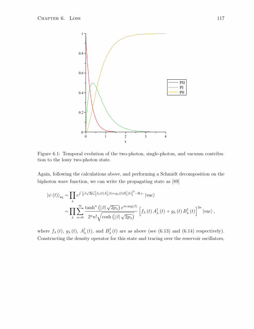
Chapter 6. Loss 117
Figure 6.1: Temporal evolution of the two-photon, single-photon, and vacuum contribu-tion to the lossy two-photon state.
Again, following the calculations above, and performing a Schmidt decomposition on the
biphoton wave function, we can write the propagating state as [89]
|ψ (t)⟩sq =∏λ
e∫
12β√2pλ[fλ(t)A†
λ(t)+gλ(t)B†λ(t)]
2−H.c. |vac⟩
=∏λ
∞∑n=0
tanhn(|β|
√2pλ)ein arg(β)
2nn!√
cosh(|β|
√2pλ) [
fλ (t)A†λ (t) + gλ (t)B†
λ (t)]2n
|vac⟩ ,
where fλ (t), gλ (t), A†λ (t), and B†
λ (t) are as above (see (6.13) and (6.14) respectively).
Constructing the density operator for this state and tracing over the reservoir oscillators,
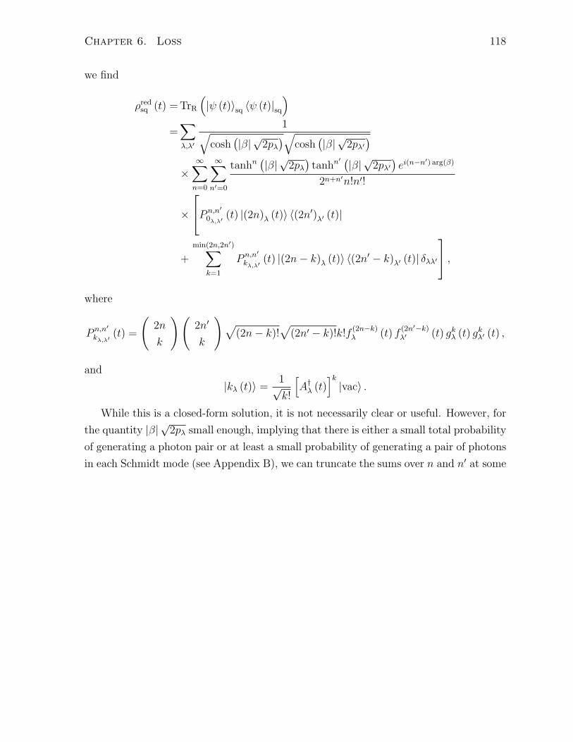
Chapter 6. Loss 118
we find
ρredsq (t) = TrR
(|ψ (t)⟩sq ⟨ψ (t)|sq
)=∑λ,λ′
1√cosh
(|β|
√2pλ)√
cosh(|β|
√2pλ′
)×
∞∑n=0
∞∑n′=0
tanhn(|β|
√2pλ)
tanhn′ (|β|√2pλ′)ei(n−n′) arg(β)
2n+n′n!n′!
×
P n,n′
0λ,λ′(t) |(2n)λ (t)⟩ ⟨(2n′)λ′ (t)|
+
min(2n,2n′)∑k=1
P n,n′
kλ,λ′(t) |(2n− k)λ (t)⟩ ⟨(2n′ − k)λ′ (t)| δλλ′
,where
P n,n′
kλ,λ′(t) =
(2n
k
)(2n′
k
)√(2n− k)!
√(2n′ − k)!k!f
(2n−k)λ (t) f
(2n′−k)λ′ (t) gkλ (t) gkλ′ (t) ,
and
|kλ (t)⟩ =1√k!
[A†
λ (t)]k
|vac⟩ .
While this is a closed-form solution, it is not necessarily clear or useful. However, for
the quantity |β|√
2pλ small enough, implying that there is either a small total probability
of generating a photon pair or at least a small probability of generating a pair of photons
in each Schmidt mode (see Appendix B), we can truncate the sums over n and n′ at some
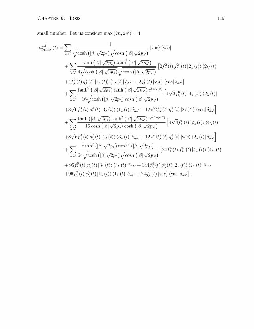
Chapter 6. Loss 119
small number. Let us consider max (2n, 2n′) = 4.
ρred2-pairs (t) =∑λ,λ′
1√cosh
(|β|
√2pλ)√
cosh(|β|
√2pλ′
) |vac⟩ ⟨vac|
+∑λ,λ′
tanh(|β|
√2pλ)
tanh′ (|β|√2pλ′
)4√
cosh(|β|
√2pλ)√
cosh(|β|
√2pλ′
) [2f 2λ (t) f 2
λ′ (t) |2λ (t)⟩ ⟨2λ′ (t)|
+4f 2λ (t) g2λ (t) |1λ (t)⟩ ⟨1λ (t)| δλλ′ + 2g4λ (t) |vac⟩ ⟨vac| δλλ′
]+∑λ,λ′
tanh2(|β|
√2pλ)
tanh(|β|
√2pλ′
)ei arg(β)
16√
cosh(|β|
√2pλ)
cosh(|β|
√2pλ′
) [4√
3f 6λ (t) |4λ (t)⟩ ⟨2λ (t)|
+8√
6f 4λ (t) g2λ (t) |3λ (t)⟩ ⟨1λ (t)| δλλ′ + 12
√2f 2
λ (t) g4λ (t) |2λ (t)⟩ ⟨vac| δλλ′
]+∑λ,λ′
tanh(|β|
√2pλ)
tanh2(|β|
√2pλ′
)e−i arg(β)
16 cosh(|β|
√2pλ)
cosh(|β|
√2pλ′
) [4√
3f 6λ (t) |2λ (t)⟩ ⟨4λ (t)|
+8√
6f 4λ (t) g2λ (t) |1λ (t)⟩ ⟨3λ (t)| δλλ′ + 12
√2f 2
λ (t) g4λ (t) |vac⟩ ⟨2λ (t)| δλλ′
]+∑λ,λ′
tanh2(|β|
√2pλ)
tanh2(|β|
√2pλ′
)64√
cosh(|β|
√2pλ)√
cosh(|β|
√2pλ′
) [24f 4λ (t) f 4
λ′ (t) |4λ (t)⟩ ⟨4λ′ (t)|
+ 96f 6λ (t) g2λ (t) |3λ (t)⟩ ⟨3λ (t)| δλλ′ + 144f 4
λ (t) g4λ (t) |2λ (t)⟩ ⟨2λ (t)| δλλ′
+96f 2λ (t) g6λ (t) |1λ (t)⟩ ⟨1λ (t)| δλλ′ + 24g8λ (t) |vac⟩ ⟨vac| δλλ′
],
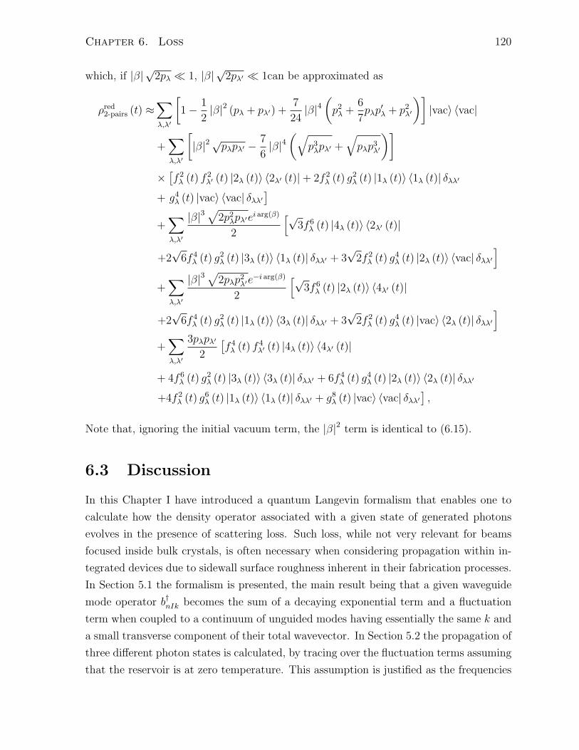
Chapter 6. Loss 120
which, if |β|√
2pλ ≪ 1, |β|√
2pλ′ ≪ 1can be approximated as
ρred2-pairs (t) ≈∑λ,λ′
[1 − 1
2|β|2 (pλ + pλ′) +
7
24|β|4
(p2λ +
6
7pλp
′λ + p2λ′
)]|vac⟩ ⟨vac|
+∑λ,λ′
[|β|2√pλpλ′ − 7
6|β|4
(√p3λpλ′ +
√pλp3λ′
)]×[f 2λ (t) f 2
λ′ (t) |2λ (t)⟩ ⟨2λ′ (t)| + 2f 2λ (t) g2λ (t) |1λ (t)⟩ ⟨1λ (t)| δλλ′
+ g4λ (t) |vac⟩ ⟨vac| δλλ′]
+∑λ,λ′
|β|3√
2p2λpλ′ei arg(β)
2
[√3f 6
λ (t) |4λ (t)⟩ ⟨2λ′ (t)|
+2√
6f 4λ (t) g2λ (t) |3λ (t)⟩ ⟨1λ (t)| δλλ′ + 3
√2f 2
λ (t) g4λ (t) |2λ (t)⟩ ⟨vac| δλλ′
]+∑λ,λ′
|β|3√
2pλp2λ′e−i arg(β)
2
[√3f 6
λ (t) |2λ (t)⟩ ⟨4λ′ (t)|
+2√
6f 4λ (t) g2λ (t) |1λ (t)⟩ ⟨3λ (t)| δλλ′ + 3
√2f 2
λ (t) g4λ (t) |vac⟩ ⟨2λ (t)| δλλ′
]+∑λ,λ′
3pλpλ′
2
[f 4λ (t) f 4
λ′ (t) |4λ (t)⟩ ⟨4λ′ (t)|
+ 4f 6λ (t) g2λ (t) |3λ (t)⟩ ⟨3λ (t)| δλλ′ + 6f 4
λ (t) g4λ (t) |2λ (t)⟩ ⟨2λ (t)| δλλ′
+4f 2λ (t) g6λ (t) |1λ (t)⟩ ⟨1λ (t)| δλλ′ + g8λ (t) |vac⟩ ⟨vac| δλλ′
],
Note that, ignoring the initial vacuum term, the |β|2 term is identical to (6.15).
6.3 Discussion
In this Chapter I have introduced a quantum Langevin formalism that enables one to
calculate how the density operator associated with a given state of generated photons
evolves in the presence of scattering loss. Such loss, while not very relevant for beams
focused inside bulk crystals, is often necessary when considering propagation within in-
tegrated devices due to sidewall surface roughness inherent in their fabrication processes.
In Section 5.1 the formalism is presented, the main result being that a given waveguide
mode operator b†nIk becomes the sum of a decaying exponential term and a fluctuation
term when coupled to a continuum of unguided modes having essentially the same k and
a small transverse component of their total wavevector. In Section 5.2 the propagation of
three different photon states is calculated, by tracing over the fluctuation terms assuming
that the reservoir is at zero temperature. This assumption is justified as the frequencies
Chapter 6. Loss 121
of interest in the waveguide are at a much higher blackbody radiation temperature than
room temperature. It also ensures that mode mixing is limited, such that there is no
photon decoherence time that is shorter than any photon loss time.
It is shown that a coherent state decays exponentially and stays coherent, and that
the “two-photon” portion of a two-photon density operator decays twice as fast as a
coherent state. The evolution of the single-photon and vacuum portion of a two-photon
density operator was also calculated and plotted in Fig. 6.1. For a given Schmidt mode,
λ, the single-photon probability reaches a maximum value of 1/2 when βλt = ln (2) /2,
at which point it is more probable than either its associated two-photon or vacuum
density operator. For all times beyond βλt = ln (3/2), the associated vacuum density
operator is most probable, rising from 4/9 to 1. Lastly, the density operator for a
squeezed vacuum state experiencing loss, expanded in the number state basis for the
Schmidt modes in the limit of a low probability of pair production, is shown to exhibit
exactly the same statistics as a two-photon density operator. Thus it it clear that there is
nothing particularly abnormal about a quantum Langevin formalism for loss as applied to
general states of generated photons propagating in waveguide structures, and introduced
within the framework presented in Chapter 2 of this thesis. This is an important first
step towards a calculation that takes into account photon generation and scattering loss
simultaneously.
Chapter 7
Conclusion
This thesis has presented an analysis of quantum nonlinear optical phenomena in artifi-
cially structured media, specifically photon pair production via either SPDC or SFWM in
channel waveguides as well as microring resonators side-coupled to channel waveguides.
Not only are photon pair production efficiencies calculated, and cast in a form resem-
bling corresponding well-known classical nonlinear optical frequency conversion efficien-
cies, but the states of generated photons themselves, characterized by two-dimensional
spectral distribution functions called biphoton wave functions, are also calculated. This
allows for easy comparison of the utility of various sources for varied applications as well
as the optimization of proposed sources for specific applications before development is
started.
In Chapter 2 I presented a Hamiltonian formalism that leverages classical asymptotic-
in and asymptotic-out fields, in close analogy with scattering theory in quantum mechan-
ics, to expand the magnetic and electric displacement fields and field operators into sets
of modes that are useful for describing both classical and quantum nonlinear optics
problems in artificially structured media. These fields are the stationary solutions of the
classical linear Maxwell equations, and can be evaluated analytically or numerically. This
strategy places classical and corresponding quantum nonlinear optical processes on equal
theoretical footing, and simplifies problems involving cavity-like structures as it avoids
the construction of Hamiltonians for the cavity modes as well as coupling between cavity
modes and propagating modes. When considering quantum nonlinear optics problems,
the formalism takes advantage of the fact that, in the perturbative limit, the output state
is expected to consist of an undepleted pump as well as the state of generated photons;
calculating the evolution of the undepleted pump, which is often quite simple, and pulling
it aside implies that what remains in the output state must be the generated photons of
interest. Additionally, both the material and modal dispersion of the input and output
122
Chapter 7. Conclusion 123
channels are correctly accounted for.
While the formalism can consider quite general input states of light, such as Fock
states and squeezed states, of arbitrary bandwidth and duration, this thesis only con-
sidered coherent input states described by Gaussian spectral distributions. Furthermore,
evolution of the input coherent state pump was not considered using the full apparatus of
the theory and instead, as a first approximation, the pump was left unmodified. Although
it is argued in Chapter 5 that it is reasonable to neglect SPM of the pump field, XPM
of the generated fields induced by the pump field, and TPA and associated FCA caused
by the pump field when pump powers are kept low enough to ensure a low probability
of photon pair production, future work should consider what happens at higher pump
powers. Whether or not analytic forms of the pair production efficiency and biphoton
wave function could still be found remains an open question, but the formalism allows
for such quantities to be calculated numerically if not analytically in the presence of
self-and cross-phase modulation. Additionally, it would be fruitful to look beyond the
undepleted pump approximation and examine the quantum to classical transition that
occurs as generated fields begin to seed classical frequency conversion processes.
I then applied the formalism of Chapter 2 to channel waveguides and microring res-
onators to calculate DFG, SHG, and SPDC efficiencies when a second-order nonlinearity
is dominant, and FWM and SFWM efficiencies when a third-order nonlinearity is domi-
nant. Use of the same formalism to make both quantum and classical calculations enabled
links between corresponding processes to be readily apparent; I was able to show that
photon pair generation efficiencies could be cast into forms resembling well-known clas-
sical frequency conversion efficiencies. I showed that, in the long pump pulse limit and
under the undepleted pump approximation, the average energy of a generated photon
divided by a characteristic time related to the photon generation bandwidth plays the
role of the classical “seed” signal in a quantum process: the larger the possible emission
bandwidth, the larger the fluctuating power available to drive the process. This close
link between quantum and classical nonlinear optical processes also allows photon pair
production efficiencies to be calculated based on the results of classical nonlinear optical
experiments, a result that was recently experimentally confirmed in silicon microring res-
onators by colleagues at the University of Pavia in Italy [18]. Furthermore, I calculated
that the scaling of these efficiencies as functions of device length L in a channel waveg-
uide and resonance quality factor Q in a microring resonator are different than what
might be expected from classical expressions. The generated idler power, integrated over
the entire spectrum, scales with L3/2 for both SPDC and SFWM in a channel, unless
filtered to within a narrow spectral region around the phase matching condition, in which
Chapter 7. Conclusion 124
case it scales as L2 for both SDC and SFWM in a channel waveguide, much like DFG,
SHG, and FWM in a channel waveguide. In a ring resonator DFG and FWM scale with
Q3 and Q4, respectively, as SPDC and SFWM, respectively within a sufficiently narrow
spectral region centered at the idler/signal resonance. On the other hand, SPDC gener-
ated power collected across an entire ring resonance is proportional to Q2 and SFWM
generated power to Q3, as not only are each the fields involved in a nonlinear process
enhanced by Q but the characteristic time related to the photon generation bandwidth
is also enhanced by Q.
While other results listed above have confirmed existing results in the literature, my
results for photon pair production efficiencies in microring resonators are entirely new.
The expressions, and experimental confirmation, highlight the strength and versatility
of the formalism introduced in Chapter 2. Furthermore, there is no reason why similar
comparisons between quantum and classical processes could not be derived for other
structures. It would be useful to know if the scaling with Q is peculiar to microring
resonators, or a general feature of all resonant photonic structures. The formalism could
also be used in the future to calculate efficiencies for three-photon generation, dual-pump
SFWM, or even “translation” of single photon states from one center frequency to another
with two appropriate input fields [90] in resonant and non-resonant structures.
In Chapter 4, I catalogued the shapes and orientations of possible biphoton proba-
bility densities associated with pairs of SPDC- and SFWM-generated photons in both
channel waveguides and microring resonators. Again, to the best of my knowledge, the
microring resonator results are completely new. Knowledge of these functions enables
knowledge of the spectral correlations that exist between pairs of generated photons,
and thus their suitability for various quantum information processing applications. By
examining two specific applications, namely Bell’s inequality violation and entanglement
swapping, requiring a single photon pair and two photon pairs respectively, in detail and
without “tracing over the frequency degree of freedom” as in [42] I have determined con-
ditions sufficient for each application to be successful: the biphoton wave function must
possess certain symmetries to maximally violate Bell’s inequality, and must be factorable
for perfect entanglement swapping, confirming results for bulk crystal SPDC-generated
states [40]. While there are many methods have been proposed to control these correla-
tions in channel waveguides [72, 73, 74], I have shown microring resonators to be more
naturally suited to generating essentially frequency uncorrelated photon pairs, both pic-
torially and through the development of analytic expressions for the Schmidt number
[63] of any biphoton wave function that can be approximated as a product of two general
Gaussian functions. This property of microring resonators is due to their photon gen-

Chapter 7. Conclusion 125
eration bandwidth tending to be (locally) limited by a resonance linewidth and not by
phase matching.
Unfortunately, while broad enough pump pulses incident on microring resonators can
generate nearly spectrally uncorrelated photons, a small degree of correlation still often
exists unless spectral filtering is employed. As with the scaling relationships developed
in Chapter 3, it is not known if this is a general feature of all resonant structures, or a
property specific to microring resonators. A useful future investigation would be to look
at other types of resonant structures and the biphoton probability densities that they
can produce, in addition to the power scaling relationships that hold for them.
As mentioned above, in all of the calculations of Chapters 2 and 3 I have neglected
the effects of SPM, XPM, TPA, and FCA. Terms associated with SPM and XPM arose
naturally from the Hamiltonian formalism in calculations involving a third-order nonlin-
earity, but, as a first approximation, were discarded to keep the pump unmodified as it
evolves and to keep expressions for generation efficiencies simple and intuitive. Despite
this, it was also shown in Chapter 3 that the theoretical predictions worked quite well
under a specific set of experimental conditions [18]. The worry that something important
might have been left out of the theory and the reality that such an omission did not seem
to matter in practice was reconciled in Chapter 5, where I determined that the pump
powers used in the experiment described in Chapter 3 were too low to cause significant
SPM, XPM, TPA, or FCA. Indeed, I showed that, for an appropriately designed channel
waveguide or microring resonator, many of these processes need not become important if
one works with powers low enough to suppress multi-pair production. As this is typically
the regime of interest, it seems reasonable that such processes may rarely need to be
included in theoretical treatments of realistic devices.
Scattering loss was also neglected in the calculations of Chapters 2 and 3, and so
in the final Chapter of this thesis I partially addressed how it might be included in
future work. Rather than directly tackle the problem of simultaneous photon generation
and loss, I investigated the linear loss of “already generated” states within a quantum
Langevin formalism for loss. This approach guarantees that the cannonical equal-time
bosonic commutation relations of the system operators are conserved for all times. Rather
than attempt to include such loss by hand, from say, knowledge of how a coherent state
decays when coupled to a zero-temperature reservoir, with this method I was able to
calculate the temporal evolution of the two-photon, single-photon, and vacuum pieces of
a density operator for an initial two-photon state experiencing linear scattering loss. For
a given Schmidt mode, λ, of the two-photon state, the single-photon probability reaches
a maximum value of 1/2 when βλt = ln(2)/2, where βλ is the loss parameter for the given
Chapter 7. Conclusion 126
Schmidt mode, at which point it is more probable than either its associated two-photon
or vacuum density operator. For all times beyond βλt = ln(3/2), the associated vacuum
density operator is most probable, rising from 4/9 to 1. Furthermore, I demonstrated
that such terms can be recovered from a full squeezed-vacuum state undergoing linear
scattering loss in the limit of a small probability of pair production, and calculated that,
within such a model, decoherence does not occur any faster than the decay of the lossiest
Schmidt mode. This can be understood by recalling that a zero-temperature reservoir
limits mode mixing.
This suggests that there is nothing pathological about linear scattering loss on general
photonic states, and serves as a first step to the introduction of such loss within the
formalism introduced at the start of this thesis. A challenge will be how to reconcile the
instantaneous nature of the scattering theory approach to photon generation of Chapter
2 with the continuous nature of the loss experienced by photon states of Chapter 6, but
a possible work-around could involve the use of reservoir oscillators that are defined with
respect to spatial coordinates rather than k-space coordinates.
Appendix A
Evolution Operator Identities
Here we consider evolution operators that specify the formal solution
|ψ (t)⟩ = U (t, t′) |ψ (t′)⟩ , (A.1)
to the time-dependent Schrodinger equation
i~d
dt|ψ (t)⟩ = H (t) |ψ (t)⟩ , (A.2)
defined such that
U(t0, t0) = I, (A.3)
for some initial t0. By taking appropriate partial derivatives of (A.1) and substituting
(A.2) we find
i~∂U(t, t′)
∂t=H(t)U(t, t′),
i~∂U(t, t′)
∂t′= − U(t, t′)H(t′), (A.4)
or
dU(t, t′) =
(1
i~H(t)U(t, t′)
)dt+
(− 1
i~U(t, t′)H(t′)
)dt′.
For U(t, t′) to be really a function of just the two variables (t, t′), and not also on the
path in the (τ1, τ2) plane used to get from (τ, τ) to the (t, t′) of interest, this must be a
total derivative. That is, we must have
∂
∂t′
(1
i~H(t)U(t, t′)
)=
∂
∂t
(− 1
i~U(t, t′)H(t′)
), (A.5)
127
Appendix A. Evolution Operator Identities 128
and using (A.4) it is easy to see that this is satisfied. So this evolution (A.4) can be used
to together with (A.3) to map out a unique U(t, t′) for each (t, t′). Note that, viewing
(A.5) as a fundamental, required property of U(t, t′), we could have just as easily started
our discussion assuming U(t, t′) to have the properties (A.4) in the absence of any kets,
instead of assuming (A.1) and (A.2).
Other properties of U(t, t′) follow from (A.3) and (A.4). First note that
d
dτU(τ, τ) =
(∂U(t, t′)
∂t
)t=t′=τ
+
(∂U(t, t′)
∂t′
)t=t′=τ
=
(1
i~H(t)U(t, t′)
)t=t′=τ
+
(− 1
i~U(t, t′)H(t2)
)t=t′=τ
=1
i~[H(τ), U(τ, τ)] . (A.6)
From (A.3) we have that (d
dτU(τ, τ)
)t=t0
= 0,
and taking the derivative of (A.6) and using that expression itself we find
d2
dt2U(t, t) =
1
i~
[dH(t)
dt, U(t, t)
]− 1
~2[H(t), [H(t), U(t, t)]] ,
and so (d2
dt2U(t, t)
)t=t0
= 0,
and so on for all higher derivatives. So we have
U(t, t) = I, (A.7)
for all t, not just t0.
Next we look at
∂
∂t
(U †(t, t′)U(t, t′
)) =
1
i~U †(t, t′)H(t)U(t, t′) − 1
i~U †(t, t′)H(t)U(t, t′) = 0,
where we have used the adjoint of the first of (A.4) and the fact that H(t) is Hermitian.
All higher derivatives vanish, and since U †(t′, t′)U(t′, t′) = I by virtue of (A.7), we see
that
U †(t, t′)U(t, t′) = U(t, t′)U †(t, t′) = I, (A.8)
for all t and t′, where the second of these follows from an argument similar to the first.
Appendix A. Evolution Operator Identities 129
So the operator U(t, t′) is unitary for all (t, t′).
Finally, we look at
∂
∂t′(U(t, t′)U(t′, t′′)) = − 1
i~U(t, t′)H(t′)U(t′, t′′) +
1
i~U(t, t′)H(t′)U(t′, t′′) = 0,
where we have used (A.4), and since all higher derivatives also vanish we can write that
U(t, t′)U(t′, t′′) = U(t, t′′)U(t′′, t′′). The latter is just U(t, t′′) by virtue of (A.7), and so
we have
U(t, t′)U(t′, t′′) = U(t, t′′) (A.9)
for all t2. A special case of this is
U(t, t′)U(t′, t) = I,
and right-multiplying by U †(t′, t) and using (A.8) we find
U(t, t′) = U †(t′, t). (A.10)
Appendix B
The CW Limit
We consider a state of generated photons of the form
|ψgen⟩ = exp(βC†
II − H.c.)|vac⟩ , (B.1)
where, neglecting the output (right) channel index R,
C†II |vac⟩ =
1√2
∫ ∞
0
dω1
∫ ∞
0
dω2ϕ (ω1, ω2) b†ω1b†ω2
|vac⟩ ,
is a normalized two-photon state characterized by the (normalized) BWF ϕ (ω1, ω2). We
perform a Schmidt decomposition of the BWF [63], so that
ϕ (ω1, ω2) =∑λ
√pλΦλ (ω1) Φλ (ω2) ,
where Φλ is a complete set of orthonormal functions, and the probabilities sum to 1
i.e.
∫dωΦ∗
λ (ω) Φλ′ (ω) =δλλ′ ,∑λ
Φλ (ω) Φ∗λ (ω′) =δ (ω − ω′) ,∑λ
pλ =1,
130
Appendix B. The CW Limit 131
and we also have
A†λ =
∫dωΦλ (ω) b†ω∑
λ
Φ∗λ (ω′)A†
λ =
∫dω∑λ
Φ∗λ (ω′) Φλ (ω) b†ω
=b†ω′
b†ω =∑λ
Φ∗λ (ω)A†
λ. (B.2)
As a quick aside, note that for a double Gaussian BWF
ϕ (ω1, ω2) =
√2
πσ+σ−e− (ω1−ω2)
2
2σ2− e
− (ω1+ω2)2
2σ2+ , (B.3)
the Schmidt decomposition can be found exactly (see Appendix D)
ϕ (ω1, ω2) =∞∑n=0
√pnΦn (ω1) Φn (ω2) ,
for σ− ≥ σ+, where
pn =nn
(n+ 1)n+1 ,
with
n =(σ+ − σ−)2
4σ+σ−.
The Schmidt decomposition allows us to write the generated state (B.1) as
|ψgen⟩ = exp
(β√2
∫ ∞
0
dω1
∫ ∞
0
dω2
∑λ
√pλΦλ (ω1) Φλ (ω2) b
†ω1b†ω2
− H.c.
)|vac⟩
=∏λ
exp
(β
√pλ2
∫ ∞
0
dω1
∫ ∞
0
dω2Φλ (ω1) Φλ (ω2) b†ω1b†ω2
− H.c.
)|vac⟩
=∏λ
exp(β√pλC
†IIλ
− H.c.)|vac⟩ ,
Appendix B. The CW Limit 132
where
C†IIλ
|vac⟩ =1√2
∫ ∞
0
dω1
∫ ∞
0
dω2Φλ (ω1) Φλ (ω2) b†ω1b†ω2
|vac⟩
=1√2A†
λA†λ |vac⟩ ,
and with this established we can now easily calculate the expectation value of the number
of photons in the output state. The number operator is, remembering (B.2),
N =
∫dωb†ωbω =
∑λ
A†λAλ,
and thus, recalling the transformations
S (z) aS† (z) = a cosh (|z|) + a†ei arg(z) sinh (|z|) ,
S (z) a†S† (z) = a† cosh (|z|) + ae−i arg(z) sinh (|z|) ,
where
S† (z) = S−1 (z) = e12(za†a†−H.c.),
we find the expectation value of the number operator to be
ND = ⟨ψgen|N |ψgen⟩
=
[⟨vac|
∏λ
S†λ
(β√
2pλ
)][∑λ′
A†λ′Aλ′
][∏λ′′
Sλ′′
(β√
2pλ′′
)|vac⟩
]=∑λ′
∏λ,λ′′
⟨vac|S†λ
(β√
2pλ
)A†
λ′Aλ′Sλ′′
(β√
2pλ′′
)|vac⟩
=∑λ
⟨vac|[A†
λ cosh(∣∣∣β√2pλ
∣∣∣)+ Aλe−i arg(β
√2pλ) sinh
(∣∣∣β√2pλ
∣∣∣)]×[Aλ cosh
(∣∣∣β√2pλ
∣∣∣)+ A†λe
i arg(β√2pλ) sinh
(∣∣∣β√2pλ
∣∣∣)] |vac⟩
=∑λ
sinh2(|β|√
2pλ
). (B.4)
Reasonable approximations lead to simple analytic forms of the BWFs associated with
various photon generation processes in various structures, from which we can approximate
a σ+ and a σ−. The form of the BWF used here for a SPDC or SFWM process in a
Appendix B. The CW Limit 133
channel waveguide is (see (3.12))
ϕC2 (ω1, ω2) =BC2 (ω1, ω2)ϕP (ω1 + ω2)
× sinc
[(ω1 + ω2 − ωP)
(1
vF− 1
vSH
)L
2
+
(ΛSHL
2− ΛFL
4
)(ω1 + ω2 − ωP)2 − ΛF
4L (ω1 − ω2)
2
],
and (see (3.32))
ϕC3 (ω1, ω2) =BC3 (ω1, ω2)
∫ ω1+ω2
0
dω
(ϕP (ω)ϕP (ω1 + ω2 − ω)
× sinc
ΛP
[(ω − ω1 + ω2
2
)2
−(ω1 − ω2
2
)2]L
),
respectively, where the BC2(3) (ω1, ω2) are benign functions of ω1 and ω2, and ϕP (ω) is
the pump pulse waveform. In a microring resonator they have a similar form, namely
(see (3.44), and (3.53))
ϕR2 (ω1, ω2) =BR2 (ω1, ω2)ϕP (ω1 + ω2)
[i (ω1 + ω2 − ωP) − vSH
|FP(ωP)|L
]−1[i (ω1 − ωF0) + vF
|FF(ωF0)|L
] [i (ω2 − ωF0) + vF
|FF(ωF0)|L
] ,
ϕR3 (ω1, ω2) =
BR3 (ω1, ω2)∫ ω1+ω2
0dω ϕP(ω)ϕP(ω1+ω2−ω)[
i(ω−ωP)−vP
|FP(ωP)|L
][i(ω1+ω2−ω−ωP)−
vP|FP(ωP)|L
][i (ω1 − ωP) + vP
|FP(ωP)|L
] [i (ω2 − ωP) + vP
|FP(ωP)|L
] .
We consider a “top hat” pulse in time, with width T and center frequency ωP
ϕP (ω) =
√T
2πsinc
((ω − ωP)
T
2
), (B.5)
Appendix B. The CW Limit 134
and, in the limit of a long pulse (see (3.34)), find
ϕC3 (ω1, ω2) ≈BC3 (ω1, ω2)
√2π
TϕP (ω1 + ω2 − ωP )
× sinc
ΛP
[(ωP − ω1 + ω2
2
)2
−(ω1 − ω2
2
)2]L
,
ϕR3 (ω1, ω2) ≈|FP (ωP)|2 L2BR3 (ω1, ω2)
√2πTϕP (ω1 + ω2 − ωP)
v2P
[i (ω1 − ωP) + vP
|FP(ωP)|L
] [i (ω2 − ωP) + vP
|FP(ωP)|L
] ,as well as (see (3.16), (3.35), (3.45), and (3.54))
∣∣βC2∣∣2 =
PPL2
PAT
3√π |ΛF|L∣∣βC3
∣∣2 = (γPPL)2T
3√π |ΛP|L
,
∣∣βR2∣∣2 =
vFL
2
PP
PA|FF (ωF0)|
2 |FP (ωP)|2 T,∣∣βR3∣∣2 =
vPL
2(γPP)2 |FP (ωP)|6 T,
for each of the four BWFs, respectively. Setting the FWHM of the absolute value
squared of the ω1 + ω2 part of (B.3) to equal the FWHM of the absolute value squared
of (B.5) we find
σ+ ≈ 2s√ln (2)T
,
and similarly find
σC2− ≈
√4s
ln (2) |ΛF|L,
σC3− ≈
√4s
ln (2) |ΛP|L,
σR2− ≈2
√ (√2 − 1
)v2F
ln (2) |FF (ωF0)|2 L2
,
σR3− ≈2
√ (√2 − 1
)v2P
ln (2) |FP (ωP)|2 L2,
where s ≈ 1.3916 is the positive root of sinc2 (x) = 0.5. In each of these four cases, as
Appendix B. The CW Limit 135
T → ∞, σ− >> σ+ and n ≈ σ−/ (4σ+), with pn ≈ n−1, or, more specifically,
nC2 ≈ T
4√s |ΛF|L
≈(pC2n
)−1,
nC3 ≈ T
4√s |ΛP|L
≈(pC3n
)−1,
nR2 ≈ TvF√√
2 − 1
4s |FF (ωF0)|L≈(pR2n
)−1,
nR3 ≈TvP√√
2 − 1
4s |FP (ωP)|L≈(pR3n
)−1.
Thus, we see that, provided β√
2pλ ≪ 1, or(PPL
2
PAT
3√π |ΛF|L
)1/2(2
4√s |ΛF|LT
)1/2
≪ 1
⇒ PP ≪(
9π
64s
)1/2 PAL2
, (B.6)((γPPL)2
T
3√π |ΛP|L
)1/2(2
4√s |ΛP|LT
)1/2
≪ 1
⇒ PP ≪(
9π
64s
)1/4
(γL)−1 , (B.7)(vFL
2
PP
PA|FF (ωF0)|
2 |FP (ωP)|2 T)1/2
(2
4s |FF (ωF0)|LTvF
√√2 − 1
)1/2
≪ 1
⇒ PP ≪
(√2 − 1
16s2
)1/2PA
L2 |FF (ωF0)|3 |FP (ωP)|2
, (B.8)
(vPL
2(γPP)2 |FP (ωP)|6 T
)1/2(
24s |FP (ωP)|LTvP
√√2 − 1
)1/2
≪ 1
⇒ PP ≪
(√2 − 1
16s2
)1/4(γL)−1
|FP (ωP)|7/2. (B.9)
which are valid even as T → ∞. If the inequality is satisfied in one of the four cases
above, then the associated number of photons (B.4) can be approximated as
ND ≈∑λ
∣∣∣β√2pλ
∣∣∣2=2 |β|2 .
Appendix C
How The Biphoton Wave Function
Affects Two Specific Experiments
If a number of identical photon pair states can be used to violate [77]
S = |E (θA, θB) − E (θA, θ′B) + E (θ′A, θB) + E (θ′A, θ
′B)| ≤ 2,
where
E (θA, θB) =C (θA, θB) + C
(θ⊥A , θ
⊥B
)− C
(θ⊥A , θB
)− C
(θA, θ
⊥B
)C (θA, θB) + C
(θ⊥A , θ
⊥B
)+ C
(θ⊥A , θB
)+ C
(θA, θ⊥B
) ,and C (θA, θB) is the number of coincidences for coincidence detection of photons passing
through linear polarizers set at an angle θi from the horizontal, H, axis, and θ⊥i = θi+π/2,
then, provided the fair sampling hypothesis is correct, at least one of the assumptions of
realism and locality that were used to derive the inequality is incorrect [11]. While the
coincidences in the preceding equations are meant to be determined experimentally, they
may be theoretically approximated as the expectation value of the linear polarization
projection operator
PθAθB ≡∫
dωdω′ |θA (ω) θB (ω′)⟩12 ⟨θA (ω) θB (ω′)|12 ,
where
|θA (ω) θB (ω′)⟩12 = cos θA cos θB |H (ω) H (ω′)⟩12 + cos θA sin θB |H (ω) V (ω′)⟩12+ sin θA cos θB |V (ω) H (ω′)⟩12 + sin θA sin θB |V (ω) V (ω′)⟩12 ,
136
Appendix C. How The Biphoton Wave Function Affects Two Specific Experiments137
or
C (θA, θB) = Tr (PθAθBρ) ,
where ρ is a density operator. Defining the four generalized Bell states
∣∣Ψ±⟩12
=1√2
∫ ∞
0
dω1
∫ ∞
0
dω2 [ϕHV (ω1, ω2) |H (ω1) V (ω2)⟩12
± ϕVH (ω1, ω2) |V (ω1) H (ω2)⟩12] ,
∣∣Φ±⟩12
=1√2
∫ ∞
0
dω1
∫ ∞
0
dω2 [ϕHH (ω1, ω2) |H (ω1) H (ω2)⟩12
± ϕVV (ω1, ω2) |V (ω1) V (ω2)⟩12] ,
normalized according to∫ ∞
0
dω1
∫ ∞
0
dω2 |ϕHV (ω1, ω2)|2 =
∫ ∞
0
dω1
∫ ∞
0
dω2 |ϕVH (ω1, ω2)|2 = 1, (C.1)
∫ ∞
0
dω1
∫ ∞
0
dω2 |ϕHH (ω1, ω2)|2 +
∫ ∞
0
dω1
∫ ∞
0
dω2 |ϕVV (ω1, ω2)|2 = 2,
ρ takes the form |Ψ+⟩ ⟨Ψ+|, |Ψ−⟩ ⟨Ψ−|, |Φ+⟩ ⟨Φ+|, or |Φ−⟩ ⟨Φ−|. Thus, we find
C (θA, θB)
= Tr (PθAθBρ)
=∑σ1,σ2
∫dΩ1dΩ2 ⟨σ1 (Ω1) σ2 (Ω2)|12 PθAθBρ |σ1 (Ω1)σ2 (Ω2)⟩12
=
12
[cos2 θA sin2 θB ± (G+G∗) cos θA sin θB sin θA cos θB
+ sin2 θA cos2 θB]
for |Ψ±⟩1212
[H cos2 θA cos2 θB ± (M +M∗) cos θA sin θB sin θA cos θB
+ V sin2 θA sin2 θB]
for |Φ±⟩12
, (C.2)
Appendix C. How The Biphoton Wave Function Affects Two Specific Experiments138
where we have used (C.1) and defined
G =
∫ ∞
0
dω1
∫ ∞
0
dω2ϕHV (ω1, ω2)ϕ∗VH (ω1, ω2) ,
H =
∫ ∞
0
dω1
∫ ∞
0
dω2 |ϕHH (ω1, ω2)|2 ,
M =
∫ ∞
0
dω1
∫ ∞
0
dω2ϕHH (ω1, ω2)ϕ∗VV (ω1, ω2) ,
V =
∫ ∞
0
dω1
∫ ∞
0
dω2 |ϕVV (ω1, ω2)|2 . (C.3)
Note that (C.2) reduces to the more familiar
C (θA, θB) =1
2sin2 (θA ± θB) ,
if and only if G+G∗ = 2 for |Ψ±⟩12, and reduces to the more familiar
C (θA, θB) =1
2cos2 (θA ∓ θB) ,
if and only if H = V = 1, as well as M + M∗ = 2 for |Φ±⟩12. If these conditions are
satisfied, maximal violation of the CHSH inequality, S = 2√
2, can be achieved for a
proper choice of θA, θB, θ′A, and θ′B. If they are not, S will be less than 2√
2, and the
inequality may not even be violated. As an example, setting θ′A−θA = π/4, θB−θA = π/8,
and θ′B − θA = 3π/8 yields S = 2√
2 for the state |Ψ−⟩12 when G = G∗ = 1.
The conditions on (C.3) above imply that the biphoton wave function posesses certain
symmetries. To see this, recall the Schwarz inequality∣∣∣∣∫ dω1dω2A (ω1, ω2)B∗ (ω1, ω2)
∣∣∣∣2 ≤ ∫ dω1dω2 |A (ω1, ω2)|2∫
dω1dω2 |B (ω1, ω2)|2 ,
the equality holding for A (ω1, ω2) ∝ B (ω1, ω2). This allows us to write
|G|2 ≤ 1,
as well as
|M |2 ≤ HV .
The first of these inequalities, combined with G+G∗ = 2, implies that G is real and thus
Appendix C. How The Biphoton Wave Function Affects Two Specific Experiments139
|Ψ±⟩12 behaves like the idealized single-mode Bell states
1√2
(|HV⟩12 ± |VH⟩12) ,
in general (rank-1) local polarization measurements if and only if
ϕHV (ω1, ω2) = ϕVH (ω1, ω2) . (C.4)
Similarly, |M |2 ≤ HV combined with H = V = 1 and M + M∗ = 2, implies that M is
real and thus |Φ±⟩12 behaves like the idealized single-mode Bell states
1√2
(|HH⟩12 ± |VV⟩12) ,
in general (rank-1) local polarization measurements if and only if
ϕHH (ω1, ω2) = ϕVV (ω1, ω2) . (C.5)
Alternatively, if either of the states
∣∣Ψ±⟩01
∣∣Ψ±⟩23, (C.6)
is passed through the series of beam-splitters shown in Fig. 4.2, one might try to trigger on
detectors in specific channels such that the entanglement that existed between channels
0 and 1 (or 2 and 3) is “swapped” to channels 0 and 3. In particular, if photons are
detected in channels 6 and 7 or 8 and 9 then |Ψ+⟩01 |Ψ+⟩23 is “swapped” to |Ψ+⟩03, and
if photons are detected in channels 6 and 8 or 7 and 9 then |Ψ−⟩01 |Ψ−⟩23 is “swapped”
to |Ψ−⟩03, provided the biphoton wave function satisfies a condition shown below. Note
that with the set up of Fig. 4.2 only these two states can be successfully swapped. In fact,
when constrained to linear optical elements and classical feed-forward, assuming perfect
number-resolving photodetection, perfect distinguishability of only two of the four Bell
states is possible [76], and thus even with a different interferometric set-up only two of
the four Bell states could be successfully swapped. Therefore we focus our attention here
on the states (C.6). To pass the photons in channels 1 and 2 through the input arms of
Appendix C. How The Biphoton Wave Function Affects Two Specific Experiments140
a 50/50 beam-splitter is to make the transformation
bAω;1 →1√2
(bAω;5 − ibAω;4)
bAω;2 →1√2
(bAω;4 − ibAω;5) ,
and to pass each output from the 50/50 beam-splitter through a polarization beam-
splitter is to make the transformation
bVω;4 → −ibVω;7, bHω;4 → bHω;6,
bVω;5 → −ibVω;8, bHω;5 → bHω;9.
Thus, dropping the integration limits for ease of notation, the states (C.6) become
∣∣Ψ±⟩01
∣∣Ψ±⟩23
→1
4
∫dω1dω2dω
′1dω
′2 ϕHV (ω1, ω2)ϕHV (ω′
1, ω′2)
× [−i |H (ω1) V (ω2) H (ω′1) V (ω′
2)⟩0863 − |H (ω1) V (ω2) H (ω′1) V (ω′
2)⟩0893− |H (ω1) V (ω2) H (ω′
1) V (ω′2)⟩0763 + i |H (ω1) V (ω2) H (ω′
1) V (ω′2)⟩0793]
± ϕHV (ω1, ω2)ϕVH (ω′1, ω
′2)
× [− |H (ω1) V (ω2) V (ω′1) H (ω′
2)⟩0873 + i |H (ω1) V (ω2) V (ω′1) H (ω′
2)⟩0883+i |H (ω1) V (ω2) V (ω′
1) H (ω′2)⟩0773 + |H (ω1) V (ω2) V (ω′
1) H (ω′2)⟩0783]
± ϕVH (ω1, ω2)ϕHV (ω′1, ω
′2)
× [|V (ω1) H (ω2) H (ω′1) V (ω′
2)⟩0963 − i |V (ω1) H (ω2) H (ω′1) V (ω′
2)⟩0993−i |V (ω1) H (ω2) H (ω′
1) V (ω′2)⟩0663 − |V (ω1) H (ω2) H (ω′
1) V (ω′2)⟩0693]
+ ϕVH (ω1, ω2)ϕVH (ω′1, ω
′2)
× [−i |V (ω1) H (ω2) V (ω′1) H (ω′
2)⟩0973 − |V (ω1) H (ω2) V (ω′1) H (ω′
2)⟩0983− |V (ω1) H (ω2) V (ω′
1) H (ω′2)⟩0673 + i |V (ω1) H (ω2) V (ω′
1) H (ω′2)⟩0683]
≡∣∣Ψ±⟩ .
Then two photons can be detected to project the photons in channels 0 and 3 onto the
desired state. The state that remains after such detection can be written as a reduced
density operator. For instance, if photons from |Ψ±⟩ are detected in channels 6 and 7

Appendix C. How The Biphoton Wave Function Affects Two Specific Experiments141
we find
ρ67 =1
2
∫dΩ1dΩ2dω1dω2dω3dω4
× [ϕHV (ω1,Ω2)ϕHV (Ω1, ω2)ϕ∗HV (ω3,Ω2)ϕ
∗HV (Ω1, ω4)
× |H (ω1) V (ω2)⟩03 ⟨H (ω3) V (ω4)|03+ ϕHV (ω1,Ω2)ϕHV (Ω1, ω2)ϕ
∗VH (ω3,Ω1)ϕ
∗VH (Ω2, ω4)
× |H (ω1) V (ω2)⟩03 ⟨V (ω3) H (ω4)|03+ ϕVH (ω1,Ω1)ϕVH (Ω2, ω2)ϕ
∗HV (ω3,Ω2)ϕ
∗HV (Ω1, ω4)
× |V (ω1) H (ω2)⟩03 ⟨H (ω3) V (ω4)|03+ ϕVH (ω1,Ω1)ϕVH (Ω2, ω2)ϕ
∗VH (ω3,Ω1)ϕ
∗VH (Ω2, ω4)
× |V (ω1) H (ω2)⟩03 ⟨V (ω3) H (ω4)|03] ,
where
ρnm =Trnm (Pnm |Ψ±⟩ ⟨Ψ±|)
⟨Ψ±|Pnm |Ψ±⟩,
and
Pnm =
∫dΩ1dΩ2 |H (Ω1) V (Ω2)⟩nm ⟨H (Ω1) V (Ω2)|nm ,
Similarly
ρ98 = ρ67 ≡ ρΨ+ ,
and
ρ68 = ρ97 =1
2
∫dΩ1dΩ2dω1dω2dω3dω4
× [ϕHV (ω1,Ω2)ϕHV (Ω1, ω2)ϕ∗HV (ω3,Ω2)ϕ
∗HV (Ω1, ω4)
× |H (ω1) V (ω2)⟩03 ⟨H (ω3) V (ω4)|03− ϕHV (ω1,Ω2)ϕHV (Ω1, ω2)ϕ
∗VH (ω3,Ω1)ϕ
∗VH (Ω2, ω4)
× |H (ω1) V (ω2)⟩03 ⟨V (ω3) H (ω4)|03− ϕVH (ω1,Ω1)ϕVH (Ω2, ω2)ϕ
∗HV (ω3,Ω2)ϕ
∗HV (Ω1, ω4)
× |V (ω1) H (ω2)⟩03 ⟨H (ω3) V (ω4)|03+ ϕVH (ω1,Ω1)ϕVH (Ω2, ω2)ϕ
∗VH (ω3,Ω1)ϕ
∗VH (Ω2, ω4)
× |V (ω1) H (ω2)⟩03 ⟨V (ω3) H (ω4)|03]
≡ ρΨ−
A successful entanglement swapping operation would mean that we could write the
Appendix C. How The Biphoton Wave Function Affects Two Specific Experiments142
density matrices ρΨ+ and ρΨ− as |Ψ+⟩03 ⟨Ψ+|03 and |Ψ−⟩03 ⟨Ψ−|03, respectively. To
examine the conditions necessary for this to be possible, we perform the Schmidt decom-
position
ϕHV (ω1, ω2) =∑λ
√pλΦλ (ω1) Θλ (ω2) ,
Note that the Schmidt functions are orthonormal, satisfying∫dωΦλ (ω) Φ∗
λ′ (ω) =
∫dωΘλ (ω) Θ∗
λ′ (ω) = δλλ′ ,
and that√pλ > 0∀λ with
∑λ pλ = 1. Thus, we may simplify the density matrices above
to
ρΨ± =1
2
∑λλ′
pλpλ′
∫dω1dω2dω3dω4
× [Φλ (ω1) Θλ′ (ω2) Φ∗λ (ω3) Θ∗
λ′ (ω4) |H (ω1) V (ω2)⟩03 ⟨H (ω3) V (ω4)|03± Φλ (ω1) Θλ′ (ω2) Θ∗
λ′ (ω3) Φ∗λ (ω4) |H (ω1) V (ω2)⟩03 ⟨V (ω3) H (ω4)|03
± Θλ (ω1) Φλ′ (ω2) Φ∗λ′ (ω3) Θ∗
λ (ω4) |V (ω1) H (ω2)⟩03 ⟨H (ω3) V (ω4)|03+ Θλ (ω1) Φλ′ (ω2) Θ∗
λ (ω3) Φλ′ (ω4) |V (ω1) H (ω2)⟩03 ⟨V (ω3) H (ω4)|03] ,
and calculate their fidelity [11] with |Ψ±⟩03 ⟨Ψ±|03
FΨ± =√
⟨Ψ±|03 ρΨ± |Ψ±⟩03.
We find
FΨ± =
√∑λ
p3λ,
a quantity which is less than 1 unless there is only a single Schmidt coefficient√p1 = 1.
Thus entanglement swapping can be successful for the states |Ψ±⟩01 |Ψ±⟩23 if and only if
the biphoton wave function is factorable
ϕHV (ω1, ω2) = Φ (ω1) Θ (ω2) . (C.7)
Appendix D
Analytic Expressions for the
Schmidt Number
Here we make a connection between the reduced density operator of two-dimensional
functions that are the product of two Gaussian functions, which in many cases serve
as a good approximation to a particular BWF, and the momentum representation of
the density operator of a harmonic oscillator, as the latter has well-known eigenvalues
and eigenfunctions, permitting an analytic expression for the Schmidt decomposition
[63] of said two-dimensional functions. That an analytic expression for the Schmidt
decomposition of a double-Gaussian function exists is well-known [72, 40, 91], but unlike
previous works here we provide a full and more physical derivation for very general
products of two Gaussian functions. The derivation is based on a set of unpublished
notes of John Sipe’s [92].
A harmonic oscillator of mass m and resonant frequency ω at temperature T , has
density operator
⟨p| ρHO |p′⟩ =x0
~√π
1√2n+ 1
exp
[−(2n+ 1)x20
4~2(p− p′)
2
]exp
[− x20
4~2 (2n+ 1)(p+ p′)
2
],
(D.1)
where x0 =√~/ (mω), and n = exp [~ω/ (kBT )] − 1−1, is the expected number of
excitations at temperature T where kB is Boltzmann’s constant. The eigenfunctions of
(D.1) are ∫dp′ ⟨p| ρHO |p′⟩ψn (p′) = pnψn (p′) ,
where
ψn (p) = (−i)n√
x02nn!~π1/2
exp
(−x
20p
2
2~2
)Hn
(x0p~
),
143

Appendix D. Analytic Expressions for the Schmidt Number 144
and
pn =nn
(n+ 1)n+1 ,
with Hn (x) the usual Hermite polynomials. Note that
K =
(∞∑n=0
p2n
)−1
= 2n+ 1,
and thus it can be said that the Schmidt number, K, of ⟨p| ρHO |p′⟩ is 2n + 1. The
task is now to massage the reduced density operator associated with various products of
Gaussian functions into the form of (D.1).
One such product is
ϕ (Ω1,Ω2) =
√2
πσ+σ−exp
[−(Ω1 cos θ − Ω2 sin θ)2
σ2−
]exp
[−(Ω1 sin θ + Ω2 cos θ)2
σ2+
],
(D.2)
Appendix D. Analytic Expressions for the Schmidt Number 145
for which
ρred (Ω1,Ω′1) =
∫dΩ2ϕ (Ω1,Ω2)ϕ
∗ (Ω′1,Ω2)
=2
πσ+σ−
∫dΩ2
exp
[−(Ω1 cos θ − Ω2 sin θ)2 + (Ω′
1 cos θ − Ω2 sin θ)2
σ2−
]
× exp
[−(Ω1 sin θ + Ω2 cos θ)2 + (Ω′
1 sin θ + Ω2 cos θ)2
σ2+
]
=2 exp
[−(
cos2 θ2σ2
−+ sin2 θ
2σ2+
)(Ω1 − Ω′
1)2]
πσ+σ−
×∫
dΩ2
exp
−2(
Ω2 sin θ −(
Ω1+Ω′1
2
)cos θ
)2σ2−
× exp
−2(
Ω2 cos θ +(
Ω1+Ω′1
2
)sin θ
)2σ2+
=2 exp
[−σ2
+ cos2 θ+σ2− sin2 θ
2σ2+σ2
−(Ω1 − Ω′
1)2]
πσ+σ−
∫dΩ2 exp
[−(aΩ2
2 + bΩ2 + c)]
=
√2
π(σ2+ sin2 θ + σ2
− cos2 θ) exp
[−σ2+ cos2 θ + σ2
− sin2 θ
2σ2+σ
2−
(Ω1 − Ω′1)
2
]
× exp
[− 1
2(σ2+ sin2 θ + σ2
− cos2 θ) (Ω1 + Ω′
1)2
], (D.3)
where the final equality follows from the identity∫dx exp
(−(ax2 + bx+ c
))=
√π
aexp
(b2 − 4ac
4a
), (D.4)
with
a = 2
(σ2+ sin2 θ + σ2
− cos2 θ
σ2+σ
2−
)b = 2 (Ω1 + Ω′
1) sin θ cos θ
(σ2− − σ2
+
σ2+σ
2−
)c = (Ω1 + Ω′
1)2
(cos2 θ
2σ2−
+sin2 θ
2σ2+
).
Appendix D. Analytic Expressions for the Schmidt Number 146
Comparing (D.3) with (D.1), we see that if we set
x40 =4(σ2+ cos2 θ + σ2
− sin2 θ)~4
σ2+σ
2−(σ2+ sin2 θ + σ2
− cos2 θ) ,
and
2n+ 1 =
√(σ2+ cos2 θ + σ2
− sin2 θ) (σ2+ sin2 θ + σ2
− cos2 θ)
σ+σ−,
the two expressions agree, and thus (D.2) has a Schmidt number of
K =
√(σ2+ cos2 θ + σ2
− sin2 θ) (σ2+ sin2 θ + σ2
− cos2 θ)
σ+σ−. (D.5)
Note that (D.5) reduces to the more familiar [78]
K =σ2+ + σ2
−
2σ+σ−,
when θ = π/4.
Similarly
ϕ (Ω1,Ω2) =
√2 |cos θ1 sin θ2 − sin θ1 cos θ2|
πσ1σ2
× exp
[−(Ω1 sin θ1 + Ω2 cos θ1)
2
σ21
]exp
[−(Ω1 sin θ2 + Ω2 cos θ2)
2
σ22
], (D.6)
Appendix D. Analytic Expressions for the Schmidt Number 147
has reduced density operator
ρred (Ω1,Ω′1) =
∫dΩ2ϕ (Ω1,Ω2)ϕ
∗ (Ω′1,Ω2)
=2 |cos θ1 sin θ2 − sin θ2 cos θ1|
πσ1σ2
×∫
dΩ2
exp
[−(Ω1 sin θ1 + Ω2 cos θ1)
2 + (Ω′1 cos θ1 + Ω2 sin θ1)
2
σ21
]
× exp
[−(Ω1 sin θ2 + Ω2 cos θ2)
2 + (Ω′1 sin θ2 + Ω2 cos θ2)
2
σ22
]
=2 |cos θ1 sin θ2 − sin θ2 cos θ1|
πσ1σ2exp
[−(
sin2 θ12σ2
1
+sin2 θ2
2σ22
)(Ω1 − Ω′
1)2
]
×∫
dΩ2
exp
−2(
Ω2 cos θ1 +(
Ω1+Ω′1
2
)sin θ1
)2σ21
× exp
−2(
Ω2 cos θ2 +(
Ω1+Ω′1
2
)sin θ2
)2σ22
=2 |cos θ1 sin θ2 − sin θ1 cos θ2|
πσ1σ2exp
[−σ
21 sin2 θ2 + σ2
1 sin2 θ22σ2
1σ22
(Ω1 − Ω′1)
2
]×∫
dΩ2 exp(−(aΩ2
2 + bΩ2 + c))
=
√2 (cos θ1 sin θ2 − cos θ2 sin θ1)
2
π (σ21 cos2 θ2 + σ2
2 cos2 θ1)exp
[−σ
21 sin2 θ2 + σ2
2 sin2 θ12σ2
1σ22
(Ω1 − Ω′1)
2
]× exp
[−(cos θ1 sin θ2 − cos θ2 sin θ1)
2
2 (σ21 cos2 θ2 + σ2
2 cos2 θ1)(Ω1 + Ω′
1)2
], (D.7)
where again the last equality follows from (D.4), this time with
a =2
(σ21 cos2 θ2 + σ2
2 cos2 θ1σ21σ
22
)b =2 (Ω1 + Ω′
1)
(σ21 sin θ2 cos θ2 + σ2
2 sin θ1 cos θ1σ21σ
22
)c = (Ω1 + Ω′
1)2
(sin2 θ1
2σ21
+sin2 θ2
2σ22
).
Appendix D. Analytic Expressions for the Schmidt Number 148
Comparing (D.7) and (D.1) we see that the two expressions agree if we set
x40 =4 (cos θ1 sin θ2 − cos θ2 sin θ1)
2 (σ21 sin2 θ2 + σ2
2 sin2 θ1)
(σ21 cos2 θ2 + σ2
2 cos2 θ1) ~4
(σ21 cos2 θ2 + σ2
2 cos2 θ1)2σ21σ
22
,
and
2n+ 1 =
√(σ21 sin2 θ2 + σ2
2 sin2 θ1)
(σ21 cos2 θ2 + σ2
2 cos2 θ1)
σ21σ
22 (cos θ1 sin θ2 − cos θ2 sin θ1)
2 ,
making the Schmidt number for (D.6)
K =
√(σ21 sin2 θ2 + σ2
2 sin2 θ1)
(σ21 cos2 θ2 + σ2
2 cos2 θ1)
σ21σ
22 (cos θ1 sin θ2 − cos θ2 sin θ1)
2 . (D.8)
Bibliography
[1] P. A. Franken, A. E. Hill, C. W. Peters, and G. Weinreich. Generation of optical
harmonics. Phys. Rev. Lett., 7(4):118–119, Aug 1961.
[2] Z. Yang, P. Chak, A. D. Bristow, H. M. van Driel, R. Iyer, J. S. Aitchison, A. L.
Smirl, and J. E. Sipe. Enhanced second-harmonic generation in AlGaAs microring
resonators. Opt. Lett., 32(7):826–828, Apr 2007.
[3] P. P. Absil, J. V. Hryniewicz, B. E. Little, P. S. Cho, R. A. Wilson, L. G. Joneckis,
and P.-T. Ho. Wavelength conversion in GaAs micro-ring resonators. Opt. Lett.,
25(8):554–556, Apr 2000.
[4] J. D. Jackson. Classical Electrodynamics. John Wiley & Sons Inc., New York, NY,
3rd edition, 1999.
[5] A. C. Turner, C. Manolatou, B. S. Schmidt, M. Lipson, M. A. Foster, J. E. Sharping,
and A. L. Gaeta. Tailored anomalous group-velocity dispersion in silicon channel
waveguides. Opt. Express, 14(10):4357–4362, May 2006.
[6] J. S. Bell. On the Einstein Podolsky Rosen paradox. Physics, 1(3):195–200, Nov
1964.
[7] J. F. Clauser, M. A. Horne, A. Shimony, and R. A. Holt. Proposed experiment to
test local hidden-variable theories. Phys. Rev. Lett., 23(15):880–884, Oct 1969.
[8] C. H. Bennett and G Brassard. Quantum cryptography: Public key distribution and
coin tossing. In Proceedings of the IEEE International Conference on Computers,
Systems and Signal Processing, pages 175–179. IEEE Press, Dec 1984.
[9] C. H. Bennett and S. J. Wiesner. Communication via one- and two-particle operators
on Einstein-Podolsky-Rosen states. Phys. Rev. Lett., 69(20):2881–2884, Nov 1992.
149
Bibliography 150
[10] C. H. Bennett, G. Brassard, C. Crepeau, R. Jozsa, A. Peres, and W. K. Wootters.
Teleporting an unknown quantum state via dual classical and Einstein-Podolsky-
Rosen channels. Phys. Rev. Lett., 70(13):1895–1899, Mar 1993.
[11] Michael A. Nielsen and Isaac L. Chuang. Quantum Computation and Quantum
Information. Cambridge University Press, New York, NY, 2004.
[12] D. Magde and H. Mahr. Study in ammonium dihydrogen phosphate of spontaneous
parametric interaction tunable from 4400 to 16 000 A. Phys. Rev. Lett., 18(21):905–
907, May 1967.
[13] T. Suhara, H. Okabe, and M. Fujimura. Generation of polarization-entangled pho-
tons by type-II quasi-phase-matched waveguide nonlinear-optic device. IEEE Pho-
tonic. Tech. L., 19(14):1093 –1095, Jul 2007.
[14] B. Bijlani, P. Abolghasem, and A. S. Helmy. Second harmonic generation in ridge
Bragg reflection waveguides. Appl. Phys. Lett., 92(10):101124, Mar 2008.
[15] C. Xiong, G. D. Marshall, A. Peruzzo, M. Lobino, A. S. Clark, D.-Y. Choi, S. J.
Madden, C. M. Natarajan, M. G. Tanner, R. H. Hadfield, S. N. Dorenbos, T. Zijlstra,
V. Zwiller, M. G. Thompson, J. G. Rarity, M. J. Steel, B. Luther-Davies, B. J.
Eggleton, and J. L. O’Brien. Generation of correlated photon pairs in a chalcogenide
As2S3 waveguide. Appl. Phys. Lett., 98(5):051101, Jan 2011.
[16] R. Horn, P. Abolghasem, B. J. Bijlani, D. Kang, A. S. Helmy, and G. Weihs. Mono-
lithic source of photon pairs. Phys. Rev. Lett., 108(15):153605, Apr 2012.
[17] S. Clemmen, K. Phan Huy, W. Bogaerts, R. G. Baets, Ph. Emplit, and S. Massar.
Continuous wave photon pair generation in silicon-on-insulator waveguides and ring
resonators. Opt. Express, 17(19):16558–16570, Sep 2009.
[18] S. Azzini, D. Grassani, M. Galli, L. C. Andreani, M. Sorel, M. J. Strain, L. G.
Helt, J. E. Sipe, M. Liscidini, and D. Bajoni. From classical four-wave mixing to
parametric fluorescence in silicon microring resonators. Opt. Lett., 37(18):3807–3809,
Sep 2012.
[19] E. Engin, D. Bonneau, C. M. Natarajan, A. Clark, M. G. Tanner, R. H. Hadfield,
S. N. Dorenbos, V. Zwiller, K. Ohira, N. Suzuki, H. Yoshida, N. Iizuka, M. Ezaki,
J. L. O’Brien, and M. G. Thompson. Photon pair generation in silicon micro-ring
resonator and enhancement via reverse bias, 2012. arXiv:1204.4922.
Bibliography 151
[20] W. H. Louisell, A. Yariv, and A. E. Siegman. Quantum fluctuations and noise in
parametric processes. I. Phys. Rev., 124(6):1646–1654, Dec 1961.
[21] D. A. Kleinman. Theory of optical parametric noise. Phys. Rev., 174(3):1027–1041,
Oct 1968.
[22] R. Ghosh, C. K. Hong, Z. Y. Ou, and L. Mandel. Interference of two photons in
parametric down conversion. Phys. Rev. A, 34(5):3962–3968, Nov 1986.
[23] T. E. Keller and M. H. Rubin. Theory of two-photon entanglement for sponta-
neous parametric down-conversion driven by a narrow pump pulse. Phys. Rev. A,
56(2):1534–1541, Aug 1997.
[24] P. G. Kwiat, W. A. Vareka, C. K. Hong, H. Nathel, and R. Y. Chiao. Correlated
two-photon interference in a dual-beam Michelson interferometer. Phys. Rev. A,
41(5):2910–2913, Mar 1990.
[25] M. H. Rubin, D. N. Klyshko, Y. H. Shih, and A. V. Sergienko. Theory of two-
photon entanglement in type-II optical parametric down-conversion. Phys. Rev. A,
50(6):5122–5133, Dec 1994.
[26] E. Brainis. Four-photon scattering in birefringent fibers. Phys. Rev. A, 79(2):023840,
Feb 2009.
[27] W. P. Grice and I. A. Walmsley. Spectral information and distinguishability in type-
II down-conversion with a broadband pump. Phys. Rev. A, 56(2):1627–1634, Aug
1997.
[28] Z. Yang, M. Liscidini, and J. E. Sipe. Spontaneous parametric down-conversion in
waveguides: A backward Heisenberg picture approach. Phys. Rev. A, 77(3):033808,
Mar 2008.
[29] S. M. Dutra. Cavity Quantum Electrodynamics: The Strange Theory of Light in a
Box. Wiley-Interscience, Dec 2004.
[30] C. W. Gardiner and M. J. Collett. Input and output in damped quantum systems:
Quantum stochastic differential equations and the master equation. Phys. Rev. A,
31(6):3761–3774, Jun 1985.
[31] J. E. Heebner, R. Grover, and T. Ibrahim. Optical Microresonators: Theory, Fabri-
cation, and Applications. Springer, London, 2008.
Bibliography 152
[32] Z. Yang and J. E. Sipe. Generating entangled photons via enhanced spontaneous
parametric downconversion in AlGaAs microring resonators. Opt. Lett., 32(22):3296–
3298, Nov 2007.
[33] L. G. Helt, Z. Yang, M. Liscidini, and J. E. Sipe. Spontaneous four-wave mixing in
microring resonators. Opt. Lett., 35(18):3006–3008, Sep 2010.
[34] B. J. Dalton and P. L. Knight. The standard model in cavity quantum electrody-
namics. I. General features of mode functions for a Fabry-Perot cavity. J. Mod.
Opt., 46(13):1817–1837, Nov 1999.
[35] C. Monat, A. S. Clark, C. Xiong, C. Grillet, G. D. Marshall, M. J. Steel, J. Li,
L. O’Faolain, T. F. Krauss, and B. J. Eggleton. Correlated photon-pair generation
in an ultra-compact silicon photonic crystal waveguide. In CLEO:2011 - Laser
Applications to Photonic Applications, page PDPC4. Optical Society of America,
2011.
[36] Paul L. Voss, Kahraman G. Koprulu, and Prem Kumar. Raman-noise-induced
quantum limits for χ(3) nondegenerate phase-sensitive amplification and quadra-
ture squeezing. J. Opt. Soc. Am. B, 23(4):598–610, Apr 2006.
[37] Q. Lin, F. Yaman, and Govind P. Agrawal. Photon-pair generation by four-wave
mixing in optical fibers. Opt. Lett., 31(9):1286–1288, May 2006.
[38] M. G. Banaee and Jeff F. Young. Squeezed state generation in photonic crystal
microcavities. Opt. Express, 16(25):20908–20919, Dec 2008.
[39] P. D. Drummond and J. F. Corney. Quantum noise in optical fibers. i. stochastic
equations. J. Opt. Soc. Am. B, 18(2):139–152, Feb 2001.
[40] A. B. U’Ren, K. Banaszek, and I. A. Walmsley. Photon engineering for quantum
information processing. Quantum Inf. Comput., 3(7):480–502, Oct 2003.
[41] N. Sangouard and H. Zbinden. What are single photons good for? J. Mod. Opt.,
59(17):1458–1464, Oct 2012.
[42] T. S. Humble and W. P. Grice. Effects of spectral entanglement in polarization-
entanglement swapping and type-I fusion gates. Phys. Rev. A, 77(2):022312, Feb
2008.
[43] G. P. Agrawal. Nonlinear Fiber Optics. Academic Press, Burlington, MA, 4th
edition, 2007.
Bibliography 153
[44] M. Liscidini, L. G. Helt, and J. E. Sipe. Asymptotic fields for a Hamiltonian treat-
ment of nonlinear electromagnetic phenomena. Phys. Rev. A, 85(1):013833, Jan
2012.
[45] L. G. Helt, M. Liscidini, and J. E. Sipe. How does it scale? Comparing quantum
and classical nonlinear optical processes in integrated devices. J. Opt. Soc. Am. B,
29(8):2199–2212, Aug 2012.
[46] N. A. R. Bhat and J. E. Sipe. Hamiltonian treatment of the electromagnetic field in
dispersive and absorptive structured media. Phys. Rev. A, 73(6):063808, Jun 2006.
[47] Y. S. Kim and M. E. Boz. Phase Space Picture of Quantum Mechanics: Group
Theoretical Approach. World Scientific, Singapore, 1991.
[48] R. Graham. Quantum Langevin equation and input-output fields for arbitrary linear
response. Z. Phys. B Con. Mat., 76(2):265–271, Jun 1989.
[49] S. Fan, S. E. Kocabas, and J.-T. Shen. Input-output formalism for few-photon
transport in one-dimensional nanophotonic waveguides coupled to a qubit. Phys.
Rev. A, 82(6):063821, Dec 2010.
[50] J. Imry. Introduction to Mesoscopic Physics. Mesoscopic Physics and Nanotechnol-
ogy. Oxford University Press, USA, 1997.
[51] G. Breit and H. A. Bethe. Ingoing waves in final state of scattering problems. Phys.
Rev., 93(4):888–890, Feb 1954.
[52] J. R. Taylor. Scattering Theory: The Quantum Theory of Nonrelativistic Collisions.
John Wiley & Sons, Inc., New York, NY, 1972.
[53] R. Loudon. The lossless optical beam-splitter. chapter 3.2. Oxford University Press,
3rd edition, 2000.
[54] R. Loudon. Beam-splitter input-output relations. chapter 5.7. Oxford University
Press, 3rd edition, 2000.
[55] C. K. Hong, Z. Y. Ou, and L. Mandel. Measurement of subpicosecond time intervals
between two photons by interference. Phys. Rev. Lett., 59(18):2044–2046, Nov 1987.
[56] W. Magnus. On the exponential solution of differential equations for a linear oper-
ator. Commun. Pure Appl. Math., 7(4):649–673, Nov 1954.
Bibliography 154
[57] S. Tanzilli, W. Tittel, H. De Riedmatten, H. Zbinden, P. Baldi, M. DeMicheli, D.B.
Ostrowsky, and N. Gisin. PPLN waveguide for quantum communication. Eur. Phys.
J. D, 18(2):155–160, Feb 2002.
[58] J. E. Sharping, K. F. Lee, M. A. Foster, A. C. Turner, B. S. Schmidt, M. Lipson,
A. L. Gaeta, and P. Kumar. Generation of correlated photons in nanoscale silicon
waveguides. Opt. Express, 14(25):12388–12393, Dec 2006.
[59] M. B. Nasr, S. Carrasco, B. E. A. Saleh, A. V. Sergienko, M. C. Teich, J. P. Torres,
L. Torner, D. S. Hum, and M. M. Fejer. Ultrabroadband biphotons generated via
chirped quasi-phase-matched optical parametric down-conversion. Phys. Rev. Lett.,
100(18):183601, May 2008.
[60] E. Y. Zhu, Z. Tang, L. Qian, L. G. Helt, M. Liscidini, J. E. Sipe, C. Corbari,
A. Canagasabey, M. Ibsen, and P. G. Kazansky. Direct generation of polarization-
entangled photon pairs in a poled fiber. Phys. Rev. Lett., 108(21):213902, May 2012.
[61] C. Liang, K. F. Lee, M. Medic, P. Kumar, R. H. Hadfield, and S. W. Nam. Character-
ization of fiber-generated entangled photon pairs with superconducting single-photon
detectors. Opt. Express, 15(3):1322–1327, Feb 2007.
[62] L. G. Helt, E. Y. Zhu, M. Liscidini, L. Qian, and J. E. Sipe. Proposal for in-fiber
generation of telecom-band polarization-entangled photon pairs using a periodically
poled fiber. Opt. Lett., 34(14):2138–2140, Jul 2009.
[63] C. K. Law and J. H. Eberly. Analysis and interpretation of high transverse entangle-
ment in optical parametric down conversion. Phys. Rev. Lett., 92(12):127903, Mar
2004.
[64] A. Yariv. Quantum Electronics. Wiley, New York, NY, 2nd edition, 1975.
[65] A. De Rossi, V. Berger, M. Calligaro, G. Leo, V. Ortiz, and X. Marcadet. Parametric
fluorescence in oxidized aluminum gallium arsenide waveguides. Appl. Phys. Lett.,
79(23):3758–3760, Dec 2001.
[66] M. Ferrera, L. Razzari, D. Duchesne, R. Morandotti, Z. Yang, M. Liscidini, J. E.
Sipe, S. Chu, B. E. Little, and D. J. Moss. Low-power continuous-wave nonlin-
ear optics in doped silica glass integrated waveguide structures. Nat. Photonics,
2(12):737–740, Dec 2008.
Bibliography 155
[67] A. C. Turner, M. A. Foster, A. L. Gaeta, and M. Lipson. Ultra-low power parametric
frequency conversion in a silicon microring resonator. Opt. Express, 16(7):4881–4887,
Mar 2008.
[68] M. Notomi, A. Shinya, S. Mitsugi, E. Kuramochi, and H. Ryu. Waveguides,
resonators and their coupled elements in photonic crystal slabs. Opt. Express,
12(8):1551–1561, Apr 2004.
[69] The variation of the quality factor between the signal, pump, and idler resonances
is below 2% for all four rings. The value we have taken for the quality factor in the
equations is an average of the Qs of the three resonances.
[70] V. R. Almeida and M. Lipson. Optical bistability on a silicon chip. Opt. Lett.,
29(20):2387–2389, Oct 2004.
[71] It was verified that the quadratic trend is maintained up to the maximum available
pump power if the pump wavelength is retuned to compensate for the thermo-optic
redshift of the resonances for PP > 2 mW. This implies that Q degradation due to
free carrier absorption can be neglected for all the investigated PP. The data of Fig.
2 are taken with a fixed value of the pump energy.
[72] W. P. Grice, A. B. U’Ren, and I. A. Walmsley. Eliminating frequency and space-time
correlations in multiphoton states. Phys. Rev. A, 64(6):063815, Nov 2001.
[73] J. Svozilık, M. Hendrych, A. S. Helmy, and J. P. Torres. Generation of paired
photons in a quantum separable state in Bragg reflection waveguides. Opt. Express,
19(4):3115–3123, Feb 2011.
[74] S. V. Zhukovsky, L. G. Helt, D. Kang, P. Abolghasem, A. S. Helmy, and J. E. Sipe.
Generation of maximally-polarization-entangled photons on a chip. Phys. Rev. A,
85(1):013838, Jan 2012.
[75] P. G. Kwiat, E. Waks, A. G. White, I. Appelbaum, and P. H. Eberhard. Ultrabright
source of polarization-entangled photons. Phys. Rev. A, 60(2):R773–R776, Aug 1999.
[76] P. Kok and B.W. Lovett. Introduction to Optical Quantum Information Processing.
Cambridge University Press, 2010.
[77] A. Aspect, P. Grangier, and G. Roger. Experimental realization of Einstein-
Podolsky-Rosen-Bohm Gedankenexperiment : A new violation of Bell’s inequalities.
Phys. Rev. Lett., 49(2):91–94, Jul 1982.
Bibliography 156
[78] S. V. Zhukovsky, L. G. Helt, P. Abolghasem, D. Kang, J. E. Sipe, and A. S. Helmy.
Bragg reflection waveguides as integrated sources of entangled photon pairs. J. Opt.
Soc. Am. B, 29(9):2516–2523, Sep 2012.
[79] A. M. Braczyk, T. C. Ralph, W. Helwig, and C. Silberhorn. Optimized generation of
heralded Fock states using parametric down-conversion. New J. Phys., 12(6):063001,
Jun 2010.
[80] Private communication with Dr. Agata Branczyk.
[81] C. Xiong, C. Monat, A. S. Clark, C. Grillet, G. D. Marshall, M. J. Steel, J. Li,
L. O’Faolain, T. F. Krauss, J. G. Rarity, and B. J. Eggleton. Slow-light enhanced
correlated photon pair generation in a silicon photonic crystal waveguide. Opt. Lett.,
36(17):3413–3415, Sep 2011.
[82] C. Monat, B. Corcoran, M. Ebnali-Heidari, C. Grillet, B. J. Eggleton, T. P. White,
L. O’Faolain, and T. F. Krauss. Slow light enhancement of nonlinear effects in silicon
engineered photonic crystal waveguides. Opt. Express, 17(4):2944–2953, Feb 2009.
[83] L. Yin and G. P. Agrawal. Impact of two-photon absorption on self-phase modulation
in silicon waveguides. Opt. Lett., 32(14):2031–2033, Jul 2007.
[84] G. Lindblad. On the generators of quantum dynamical semigroups. Commun. Math
Phys., 48(2):119–130, Jun 1976.
[85] E. C. G. Sudarshan. Equivalence of semiclassical and quantum mechanical descrip-
tions of statistical light beams. Phys. Rev. Lett., 10(7):277–279, Apr 1963.
[86] R. J. Glauber. Coherent and incoherent states of the radiation field. Phys. Rev.,
131(6):2766–2788, Sep 1963.
[87] H. Haken. Light: Waves, Photons, Atoms. North-Holland, 1981.
[88] H.J. Carmichael. Fokker-planck equation for the damped harmonic oscillator. In
Statistical Methods in Quantum Optics, chapter 3.1.4. Springer, 1999.
[89] D. R. Truax. Baker-Campbell-Hausdorff relations and unitarity of SU(2) and SU(1,1)
squeeze operators. Phys. Rev. D, 31(8):1988–1991, Apr 1985.
[90] H. J. McGuinness, M. G. Raymer, and C. J. McKinstrie. Theory of quantum fre-
quency translation of light in optical fiber: application to interference of two photons
of different color. Opt. Express, 19(19):17876–17907, Sep 2011.

Bibliography 157
[91] A. I. Lvovsky, W. Wasilewski, and K. Banaszek. Decomposing a pulsed optical
parametric amplifier into independent squeezers. J. Mod. Opt., 54(5):721–733, Mar
2007.
[92] J. E. Sipe. DGBiphoton. Unpublished, pages 1–15, 2004.