Embed Size (px)
DESCRIPTION
Nonlinear Programming III. Constrained Optimization Techniques. Introduction. This part of the course deals with techniques that are applicable to the solution of the constrained optimization problem: - PowerPoint PPT Presentation
Citation preview
Nonlinear Programming III
Constrained Optimization Techniques
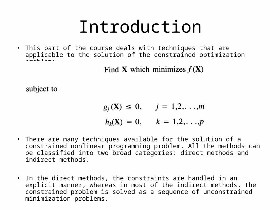
Introduction• This part of the course deals with techniques that are applicable to the
solution of the constrained optimization problem:
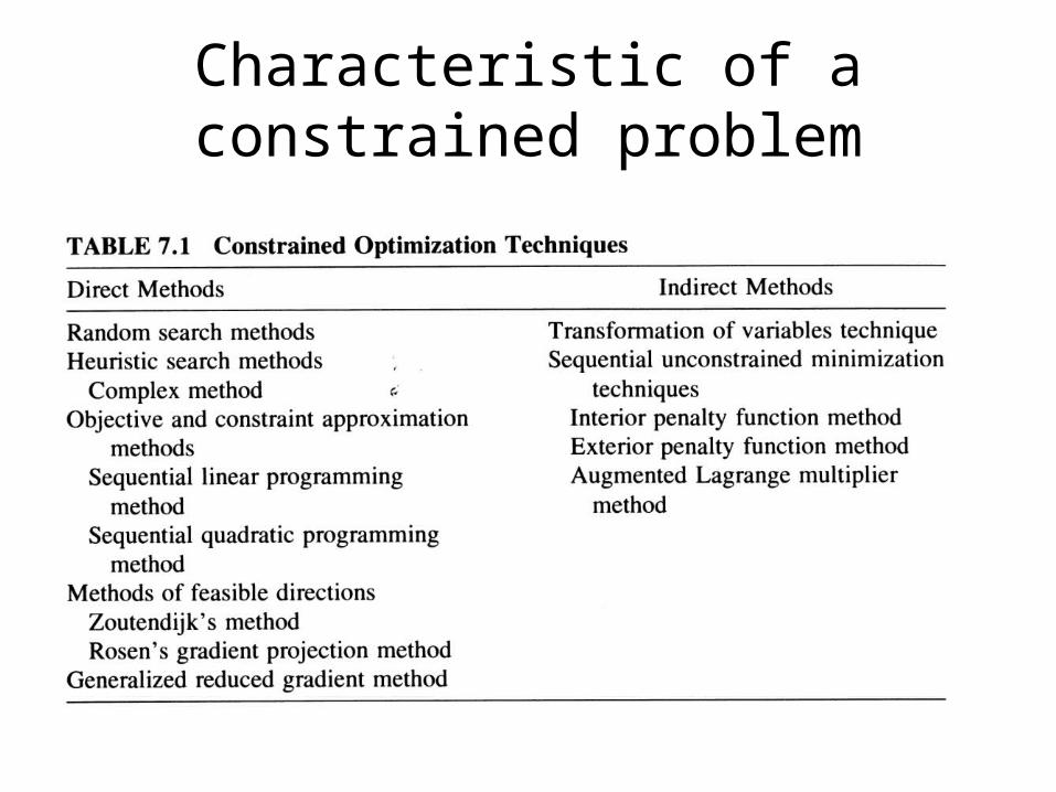
• There are many techniques available for the solution of a constrained nonlinear programming problem. All the methods can be classified into two broad categories: direct methods and indirect methods.
• In the direct methods, the constraints are handled in an explicit manner, whereas in most of the indirect methods, the constrained problem is solved as a sequence of unconstrained minimization problems.
Characteristic of a constrained problem
Characteristic of a constrained problem
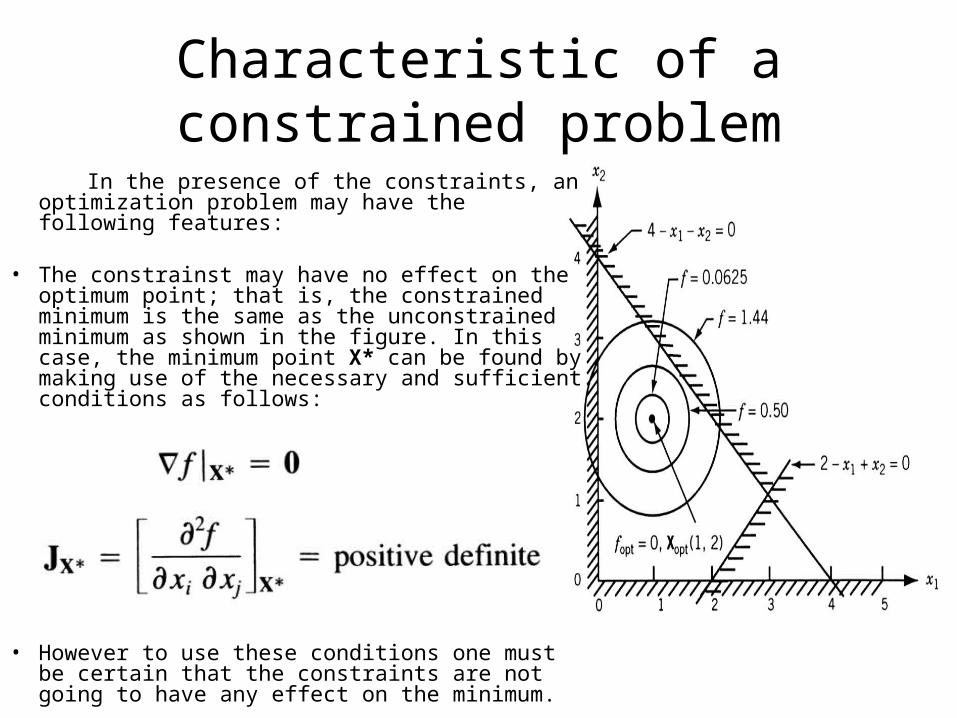
In the presence of the constraints, an optimization problem may have the following features:
• The constrainst may have no effect on the optimum point; that is, the constrained minimum is the same as the unconstrained minimum as shown in the figure. In this case, the minimum point X* can be found by making use of the necessary and sufficient conditions as follows:
• However to use these conditions one must be certain that the constraints are not going to have any effect on the minimum.
Characteristic of a constrained problem
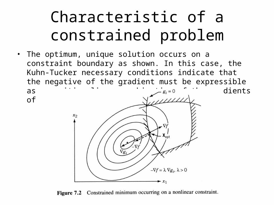
• The optimum, unique solution occurs on a constraint boundary as shown. In this case, the Kuhn-Tucker necessary conditions indicate that the negative of the gradient must be expressible as a positive linear combination of the gradients of the active constraints.
Characteristic of a constrained problem
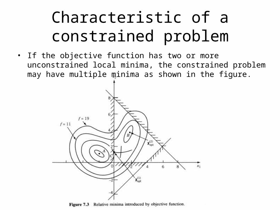
• If the objective function has two or more unconstrained local minima, the constrained problem may have multiple minima as shown in the figure.
Characteristic of a constrained problem
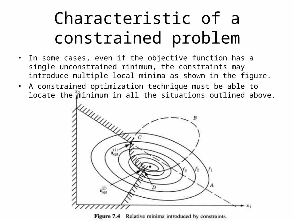
• In some cases, even if the objective function has a single unconstrained minimum, the constraints may introduce multiple local minima as shown in the figure.
• A constrained optimization technique must be able to locate the minimum in all the situations outlined above.
Direct Methods RANDOM SEARCH METHODS
The random search methods described for unconstrained minimization can be used with minor modifications to solve a constrained optimization problem. The basic procedure can be described by the following steps:
1. Generate a trial design vector using one random number for each design variable.
2. Verify whether the constraints are satisfied at the trial design vector. Usually, the equality constraints are considered satisfactory whenever their magnitudes lie within a specified tolerance. If any constraint is violated, continue generating new trial vectors until a trial vector that satisfies all the constraints is found.
3. If all the constraints are satisfied, retain the current trial vector as the best design if it gives a reduced objective function value compared to the previous best available design. Otherwise, discard the current feasible trial vector and proceed to step 1 to generate a new trial design vector.
4. The best design available at the end of generating a specified maximum number of trial design vectors is taken as the solution of the constrained optimization problem.
RANDOM SEARCH METHODS• It can be seen that several modifications can be made to the basic
procedure indicated above. For example, after finding a feasible trial design vector, a feasible direction can be generated (using random numbers) and a one-dimensional search can be conducted along the feasible direction to find an improved feasible design vector.
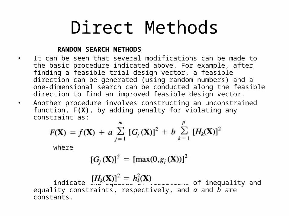
• Another procedure involves constructing an unconstrained function, F(X), by adding penalty for violating any constraint as:
where
indicate the squares of violations of inequality and equality constraints,
respectively, and a and b are constants.
Direct Methods
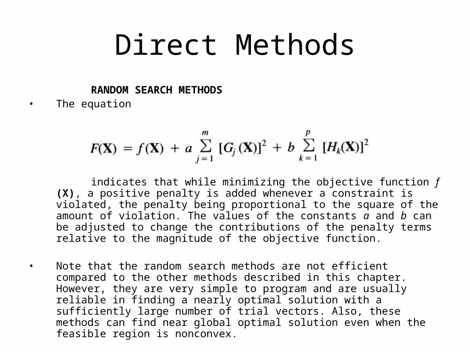
Direct Methods RANDOM SEARCH METHODS• The equation
indicates that while minimizing the objective function f (X), a positive penalty is added whenever a constraint is violated, the penalty being proportional to the square of the amount of violation. The values of the constants a and b can be adjusted to change the contributions of the penalty terms relative to the magnitude of the objective function.
• Note that the random search methods are not efficient compared to the other methods described in this chapter. However, they are very simple to program and are usually reliable in finding a nearly optimal solution with a sufficiently large number of trial vectors. Also, these methods can find near global optimal solution even when the feasible region is nonconvex.
Direct MethodsSEQUENTIAL LINEAR PROGRAMMING
• In the sequential linear programming (SLP) method, the solution of the original nonlinear programming problem is found by solving a series of linear programming problems.
• Each LP problem is generated by approximating the nonlinear objective and constraint functions using first-order Taylor series expansions about the current design vector Xi.
• The resulting LP problem is solved using the simplex method to find the new design vector Xi+1.
• If Xi+1 does not satisfy the stated convergence criteria, the problem is relinearized about the point Xi+1 and the procedure is continued until the optimum solution X* is found.
Direct Methods
SEQUENTIAL LINEAR PROGRAMMING
• If the problem is a convex programming problem, the linearized constraints always lie entirely outseide the deasible region. Hence the optimum solution of the approximating LP problem, which lies at a vertex of the new feasible region, will lie outside the original feasible region.
• However, by relinearizing the problem about the new point and repeating the process, we can achieve convergence to the solution of the original problem in a few iterations.
• The SLP method is also known as the cutting plane method.
Direct methods
SEQUENTIAL LINEAR PROGRAMMING
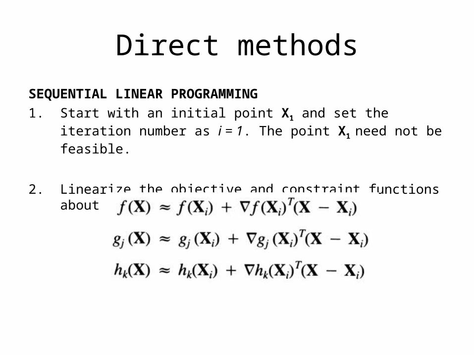
1. Start with an initial point X1 and set the iteration number as i = 1. The point X1 need not be feasible.
2. Linearize the objective and constraint functions about the point Xi as
Direct methods
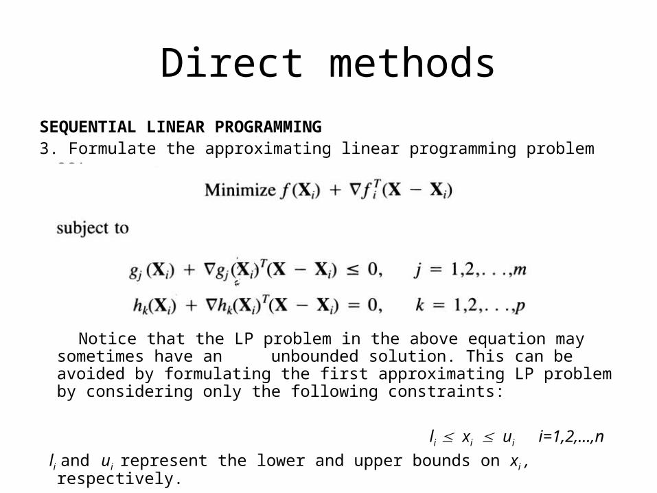
SEQUENTIAL LINEAR PROGRAMMING3. Formulate the approximating linear programming problem as:
Notice that the LP problem in the above equation may sometimes have an unbounded solution. This can be avoided by formulating the first approximating LP problem by considering only the following constraints:
li xi ui i=1,2,...,n
li and ui represent the lower and upper bounds on xi , respectively.
Direct methods
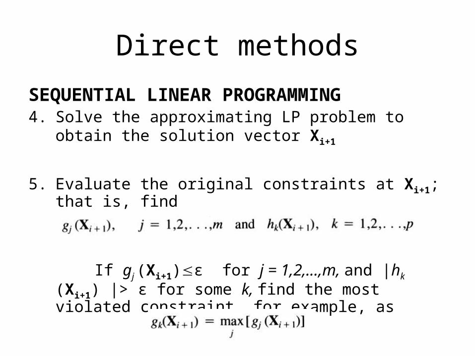
SEQUENTIAL LINEAR PROGRAMMING4. Solve the approximating LP problem to obtain the
solution vector Xi+1
5. Evaluate the original constraints at Xi+1; that is, find
If gj (Xi+1)ϵ for j = 1,2,...,m, and |hk (Xi+1) |> ϵ for some k, find the most violated constraint, for example, as
Direct methods
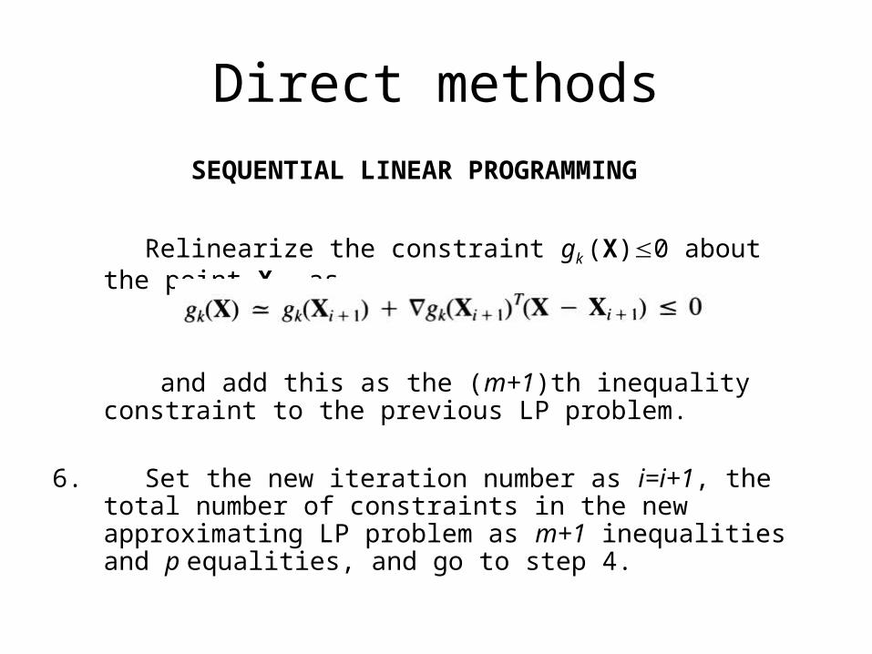
SEQUENTIAL LINEAR PROGRAMMING
Relinearize the constraint gk (X)0 about the point Xi+1 as and add this as the (m+1)th inequality constraint to the
previous LP problem.
6. Set the new iteration number as i=i+1, the total number of constraints in the new approximating LP problem as m+1 inequalities and p equalities, and go to step 4.
Direct methods
The sequential linear programming method has several advantages:
1. It is an efficient technique for solving complex programming problems with nearly linear objective functions.
2. Each of the approximating problems will be a LP problem and hence can be solved quite efficiently. Moreover, any two consecutive approximating LP problems differ by only one constraint, and hence the dual simplex method can be used to solve the sequence of approximating LP problems much more efficiently.
3. The method can easily be extended to solve integer programming problems. In this case, one integer LP problem has to be solved in each stage.
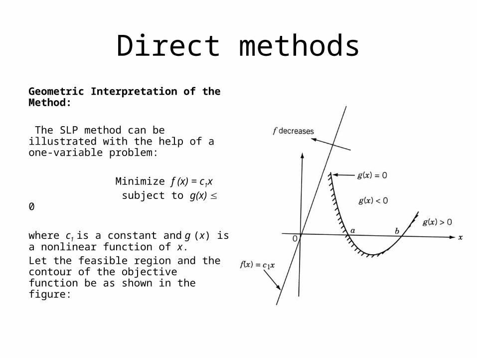
Direct methodsGeometric Interpretation of the Method:
The SLP method can be illustrated with the help of a one-variable problem:
Minimize f (x) = c1x subject to g(x) 0
where c1 is a constant and g (x) is a nonlinear function of x. Let the feasible region and the contour of the objective function be as shown in the figure:
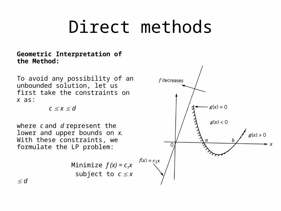
Direct methodsGeometric Interpretation of the Method:
To avoid any possibility of an unbounded solution, let us first take the constraints on x as: c x d
where c and d represent the lower and upper bounds on x. With these constraints, we formulate the LP problem:
Minimize f (x) = c1x subject to c x d
Sequential Linear Programming Problem
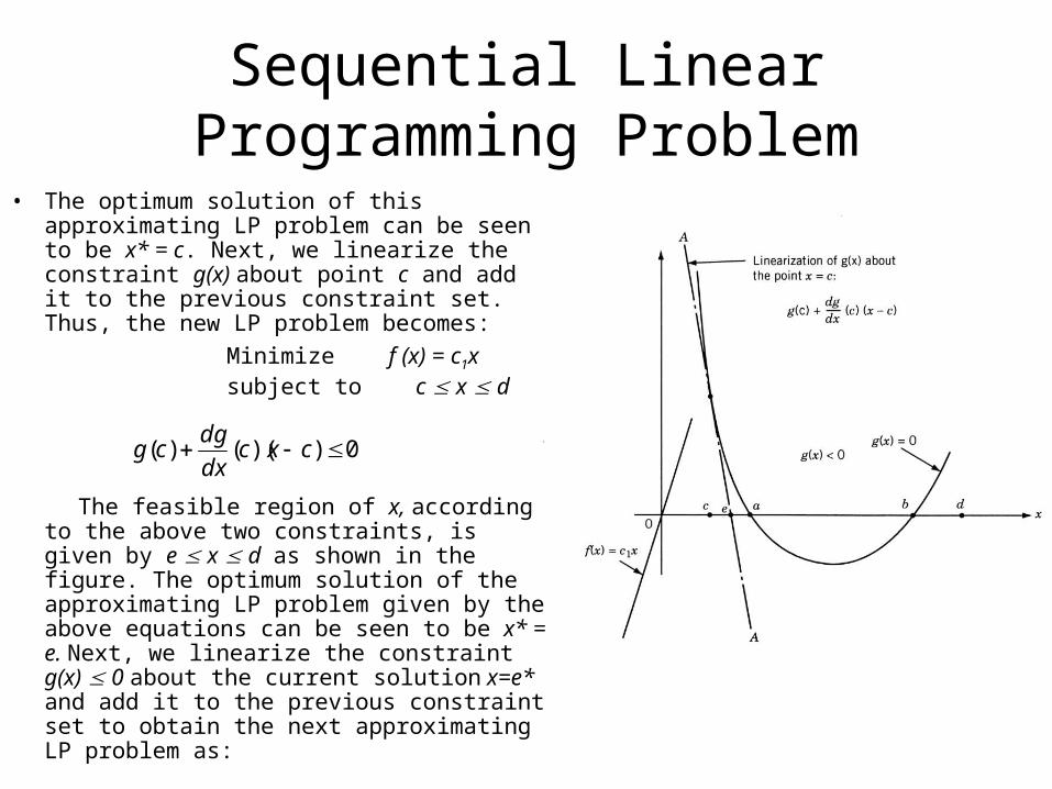
• The optimum solution of this approximating LP problem can be seen to be x* = c. Next, we linearize the constraint g(x) about point c and add it to the previous constraint set. Thus, the new LP problem becomes:
Minimize f (x) = c1x subject to c x d
The feasible region of x, according to the above
two constraints, is given by e x d as shown in the figure. The optimum solution of the approximating LP problem given by the above equations can be seen to be x* = e. Next, we linearize the constraint g(x) 0 about the current solution x=e* and add it to the previous constraint set to obtain the next approximating LP problem as:
0))(()( cxcdx
dgcg
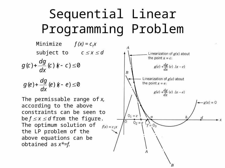
Sequential Linear Programming Problem
Minimize f (x) = c1x
subject to c x d
The permissable range of x, according to the above constraints can be seen to be f x d from the figure. The optimum solution of the LP problem of the above equations can be obtained as x*=f.
0))(()( cxcdx
dgcg
0))(()( exedx
dgeg
Sequential Linear Programming
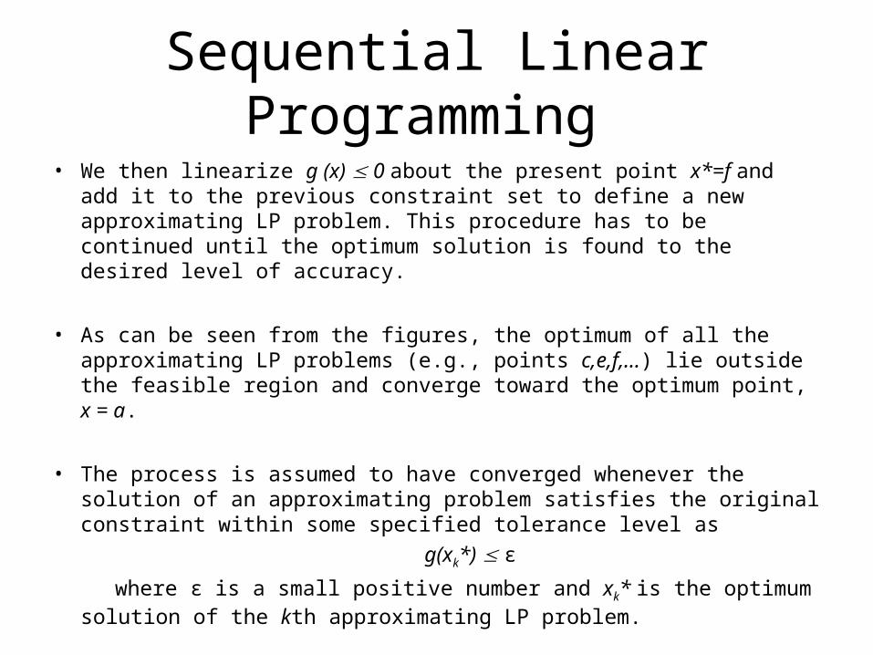
• We then linearize g (x) 0 about the present point x*=f and add it to the previous constraint set to define a new approximating LP problem. This procedure has to be continued until the optimum solution is found to the desired level of accuracy.
• As can be seen from the figures, the optimum of all the approximating LP problems (e.g., points c,e,f,...) lie outside the feasible region and converge toward the optimum point, x = a.
• The process is assumed to have converged whenever the solution of an approximating problem satisfies the original constraint within some specified tolerance level as
g(xk*) ϵ
where ϵ is a small positive number and xk* is the optimum solution of the kth approximating LP problem.
Sequential Linear Programming
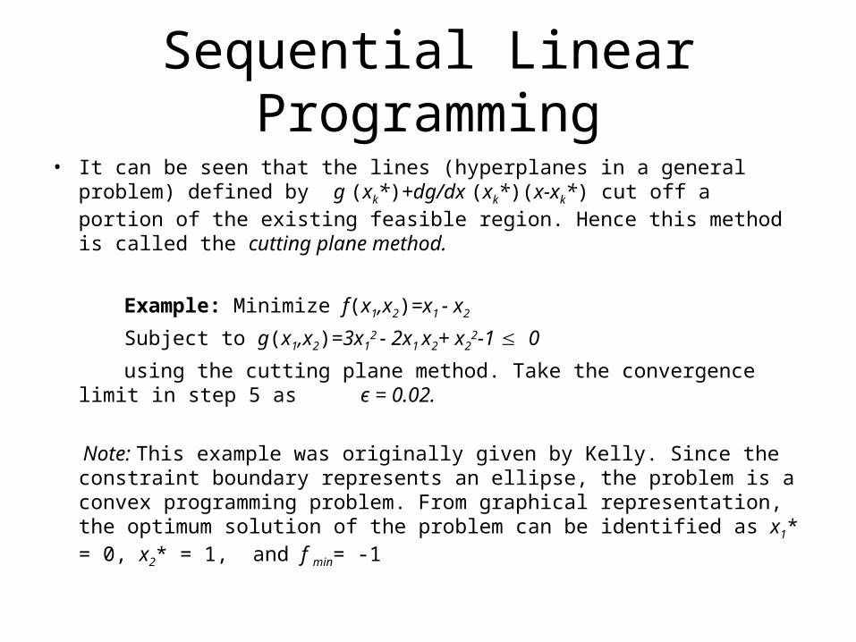
• It can be seen that the lines (hyperplanes in a general problem) defined by g (xk*)+dg/dx (xk*)(x-xk*) cut off a portion of the existing feasible region. Hence this method is called the cutting plane method.
Example: Minimize f(x1,x2)=x1 - x2
Subject to g(x1,x2)=3x12
- 2x1 x2+ x22-1 0
using the cutting plane method. Take the convergence limit in step 5 as ϵ = 0.02.
Note: This example was originally given by Kelly. Since the constraint boundary represents an ellipse, the problem is a convex programming problem. From graphical representation, the optimum solution of the problem can be identified as x1* = 0, x2* = 1, and f min= -1
Sequential Linear Programming
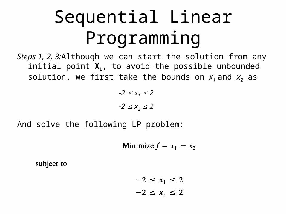
Steps 1, 2, 3:Although we can start the solution from any initial point X1, to avoid the possible unbounded solution, we first take the bounds on x1 and x2 as
And solve the following LP problem:
-2 x1 2
-2 x2 2
Sequential Linear Programming
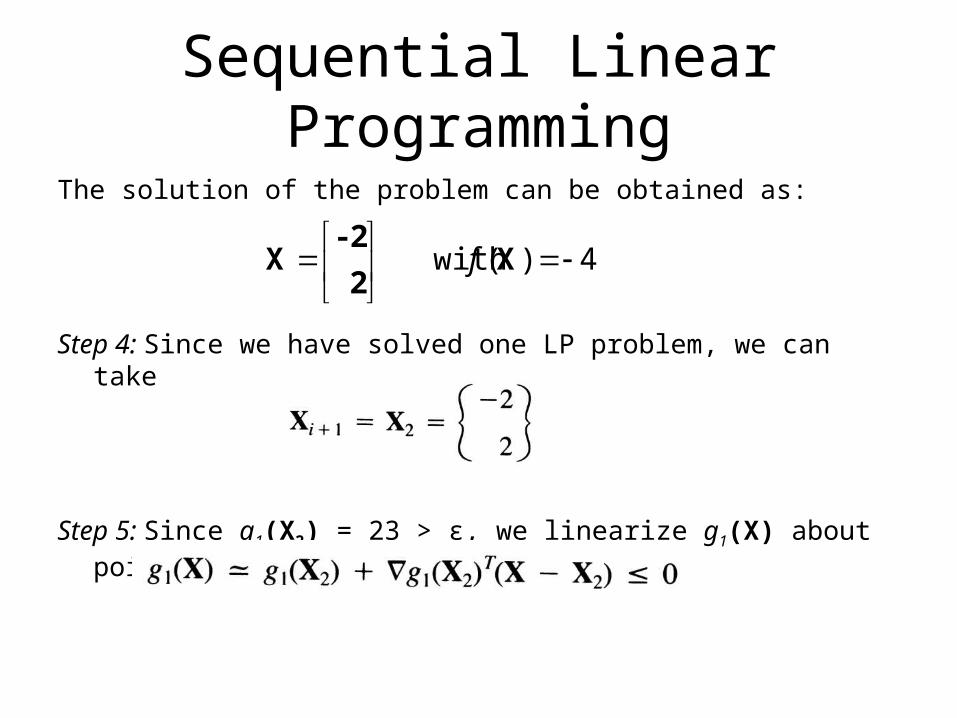
The solution of the problem can be obtained as:
Step 4: Since we have solved one LP problem, we can take
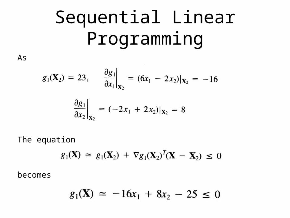
Step 5: Since g1(X2) = 23 > ϵ, we linearize g1(X) about point X2 as
4)( with
X
2
2-X f
Sequential Linear Programming
As
The equation
becomes
Sequential Linear Programming
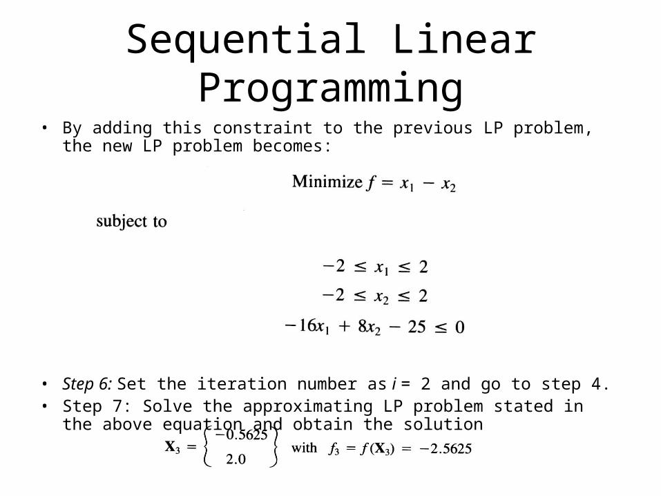
• By adding this constraint to the previous LP problem, the new LP problem becomes:
• Step 6: Set the iteration number as i = 2 and go to step 4.• Step 7: Solve the approximating LP problem stated in the above equation
and obtain the solution
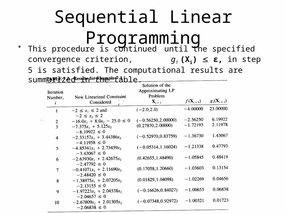
Sequential Linear Programming• This procedure is continued until the specified convergence criterion,
g1 (Xi) ϵ, in step 5 is satisfied. The computational results are summarized in the table.
Sequential Quadratic Programming
• The sequential quadratic programming is one of the most recently developed and perhaps one of the best methods of optimization.
• The method has a theoretical basis that is related to
1. The solution of a set of nonlinear equations using Newton’s method.
2. The derivation of simultaneous nonlinear equations using Kuhn-Tucker conditions to the Lagrangian of the constrained optimization problem.
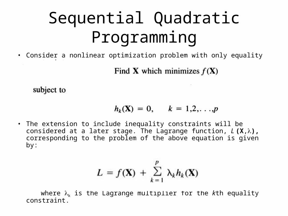
• Consider a nonlinear optimization problem with only equality constraints as:
• The extension to include inequality constraints will be considered at a later stage. The Lagrange function, L (X,), corresponding to the problem of the above equation is given by:
where k is the Lagrange multiplier for the kth equality constraint.
Sequential Quadratic Programming
Sequential Quadratic Programming
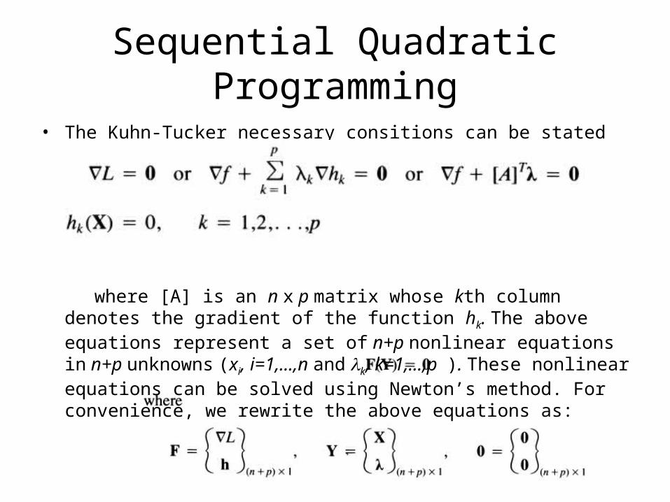
• The Kuhn-Tucker necessary consitions can be stated as:
where [A] is an n x p matrix whose kth column denotes the gradient of the function hk. The above equations represent a set of n+p nonlinear equations in n+p unknowns (xi, i=1,...,n and k, k=1,...,p ). These nonlinear equations can be solved using Newton’s method. For convenience, we rewrite the above equations as:
Sequential Quadratic Programming
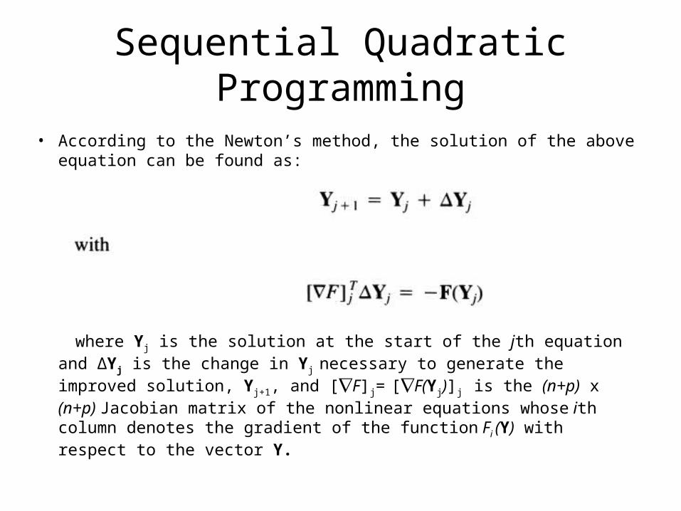
• According to the Newton’s method, the solution of the above equation can be found as:
where Yj is the solution at the start of the jth equation and ∆Yj is the change in Yj necessary to generate the improved solution, Yj+1, and [F]j=
[F(Yj)]j is the (n+p) x (n+p) Jacobian matrix of the nonlinear equations whose ith column denotes the gradient of the function Fi (Y) with respect to the vector Y.
Sequential Quadratic Programming
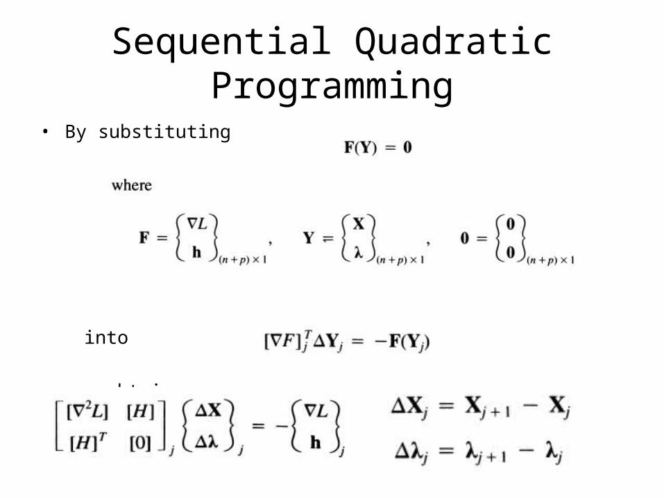
• By substituting
into
we obtain:
Sequential Quadratic Programming Method
where
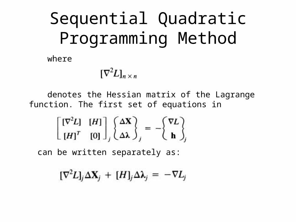
denotes the Hessian matrix of the Lagrange function. The first set of equations in
can be written separately as:
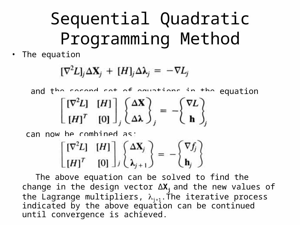
• The equation
and the second set of equations in the equation
can now be combined as:
The above equation can be solved to find the change in the design vector ∆Xj and the new values of the Lagrange multipliers, j+1.The iterative process indicated by the above equation can be continued until convergence is achieved.
Sequential Quadratic Programming Method
Sequential Quadratic Programming Method
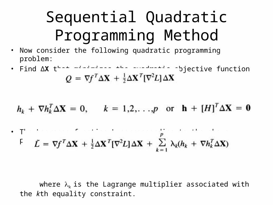
• Now consider the following quadratic programming problem:
• Find ∆X that minimizes the quadratic objective function
subject to the linear equality constraints
• The Lagrange function L corresponding to the above problem is given by:
where k is the Lagrange multiplier associated with the kth equality constraint.
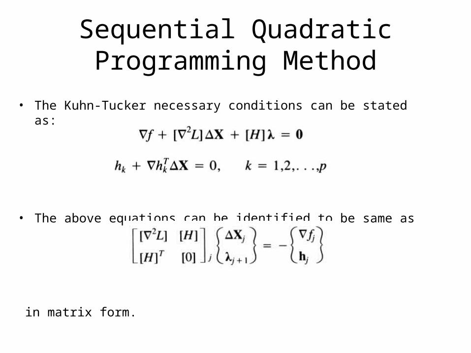
• The Kuhn-Tucker necessary conditions can be stated as:
• The above equations can be identified to be same as
in matrix form.
Sequential Quadratic Programming Method
Sequential Quadratic Programming Method
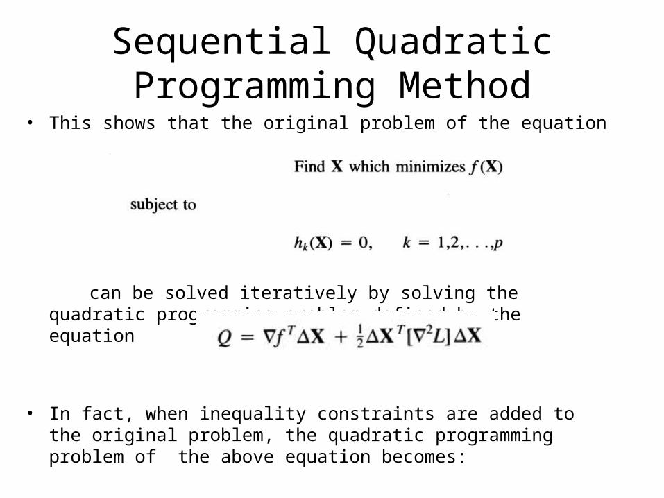
• This shows that the original problem of the equation
can be solved iteratively by solving the quadratic programming problem defined by the equation
• In fact, when inequality constraints are added to the original problem, the quadratic programming problem of the above equation becomes:
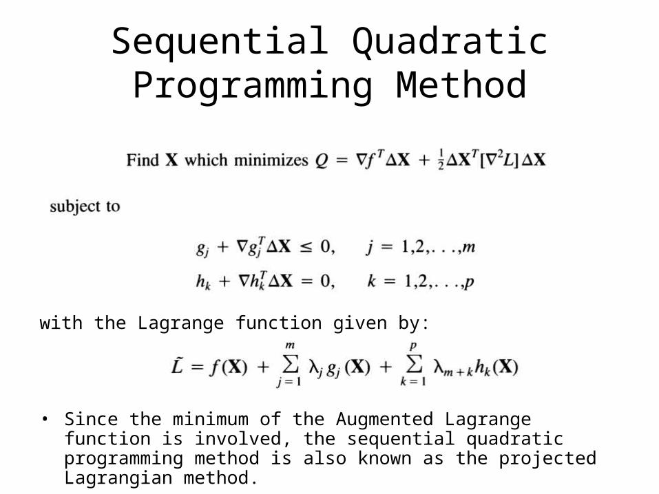
with the Lagrange function given by:
• Since the minimum of the Augmented Lagrange function is involved, the sequential quadratic programming method is also known as the projected Lagrangian method.
Sequential Quadratic Programming Method
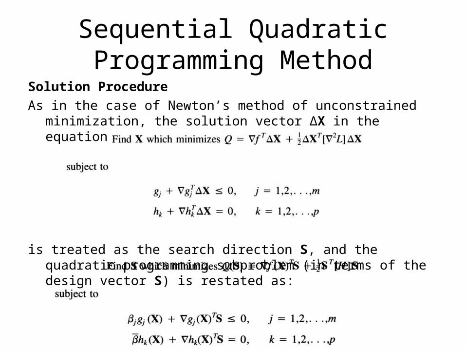
Solution Procedure
As in the case of Newton’s method of unconstrained minimization, the solution vector ∆X in the equation
is treated as the search direction S, and the quadratic programming subproblem (in terms of the design vector S) is restated as:
Sequential Quadratic Programming Method
Sequential Quadratic Programming Method
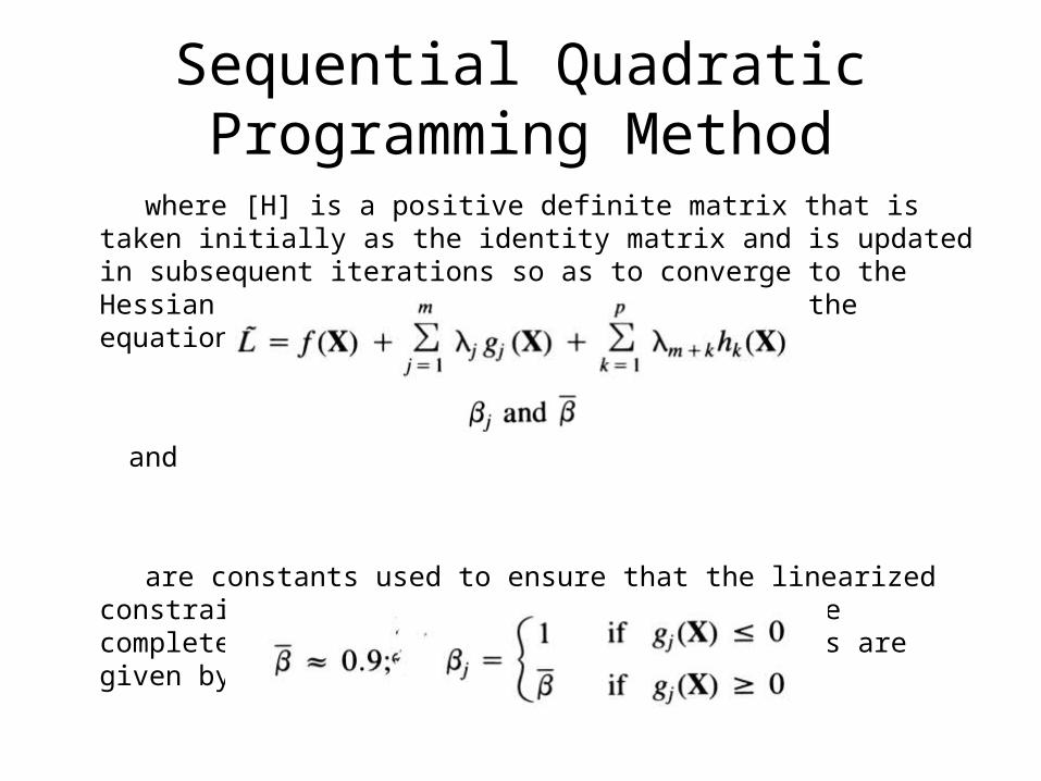
where [H] is a positive definite matrix that is taken initially as the identity matrix and is updated in subsequent iterations so as to converge to the Hessian matrix of the Lagrange function of the equation:
and
are constants used to ensure that the linearized constraints do not cut off the feasible space completely. Typical values of these constants are given by:
Sequential Quadratic Programming Method
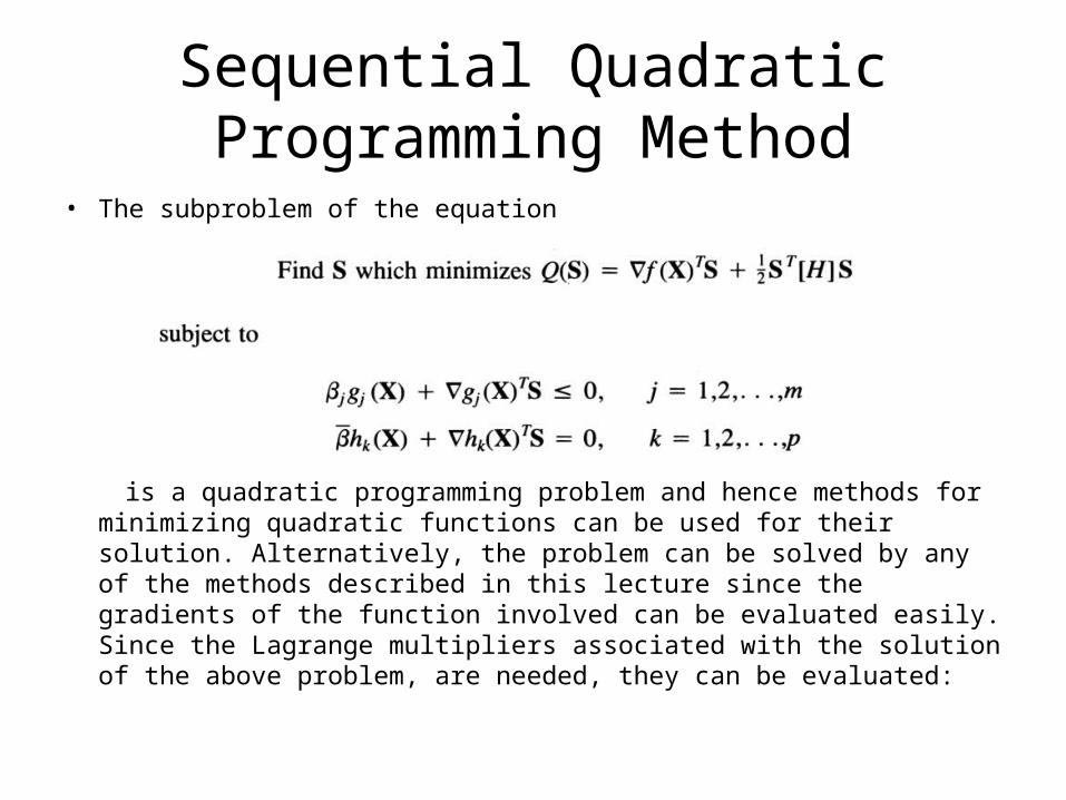
• The subproblem of the equation
is a quadratic programming problem and hence methods for minimizing quadratic functions can be used for their solution. Alternatively, the problem can be solved by any of the methods described in this lecture since the gradients of the function involved can be evaluated easily. Since the Lagrange multipliers associated with the solution of the above problem, are needed, they can be evaluated:
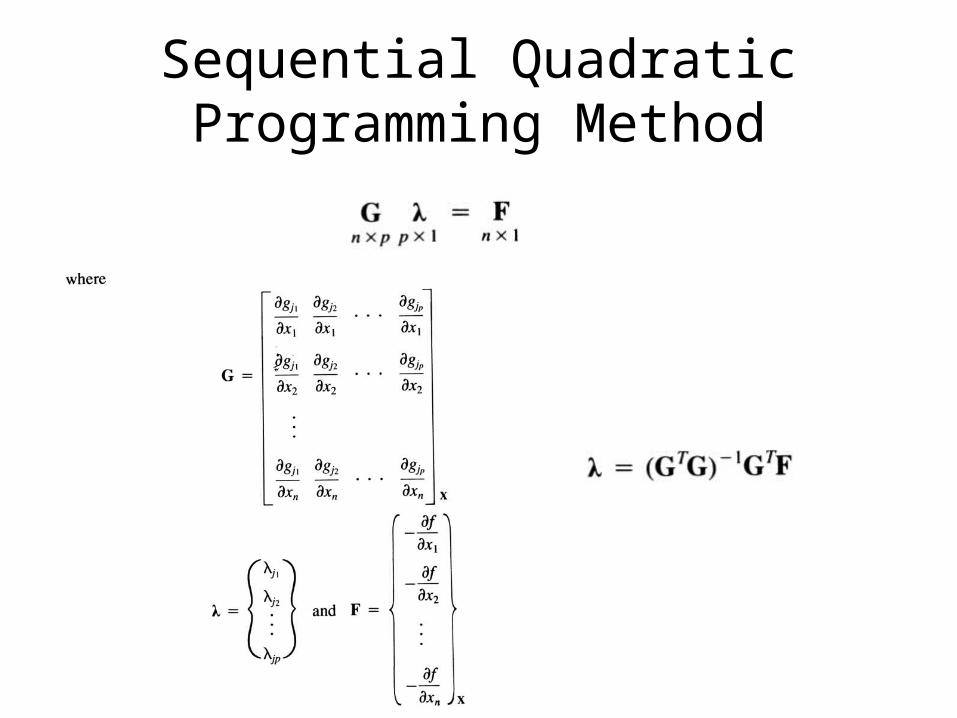
Sequential Quadratic Programming Method
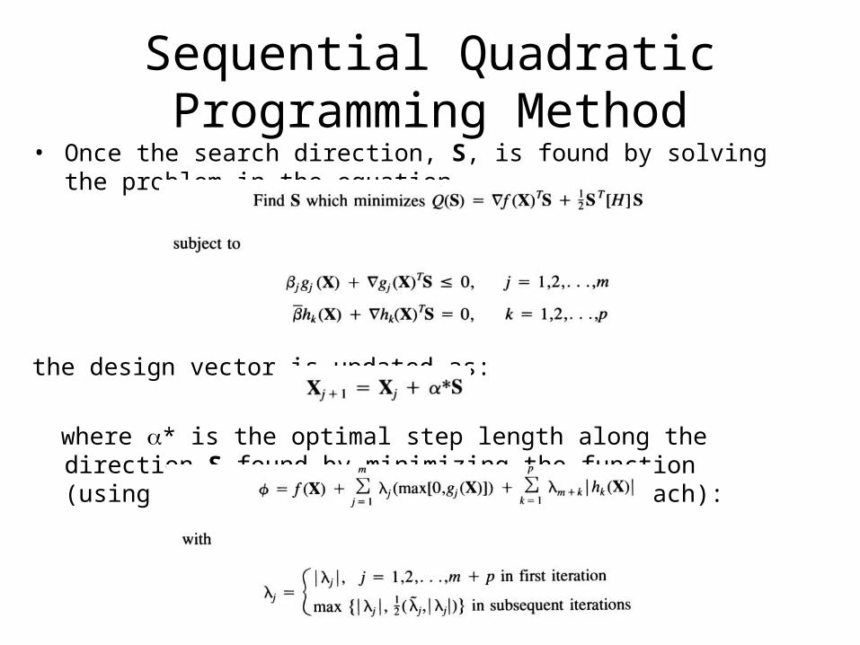
• Once the search direction, S, is found by solving the problem in the equation
the design vector is updated as:
where * is the optimal step length along the direction S found by minimizing the function (using an exterior penalty function approach):
Sequential Quadratic Programming Method
Sequential Quadratic Programming Method
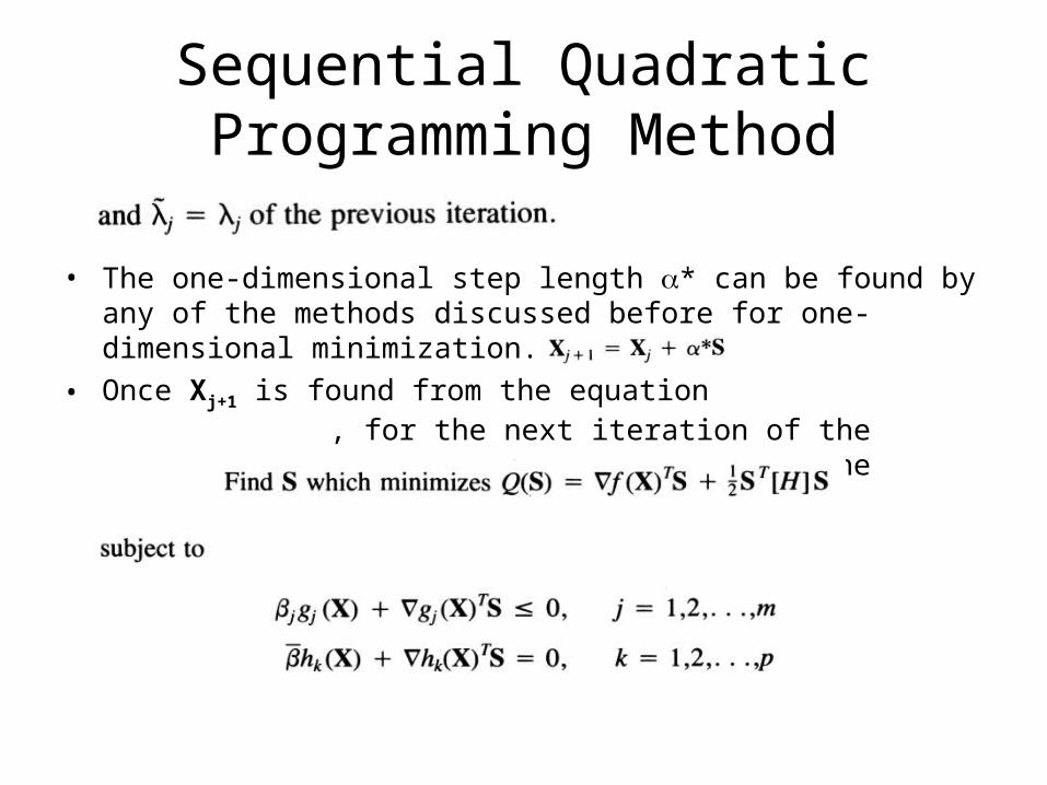
• The one-dimensional step length * can be found by any of the methods discussed before for one-dimensional minimization.
• Once Xj+1 is found from the equation , for the next iteration of the Hessian matrix [H] is updated to improve the quadratic approximation in the equation
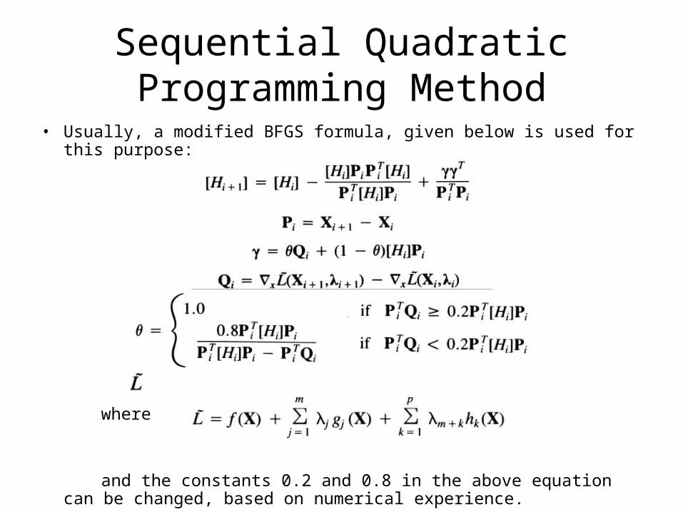
• Usually, a modified BFGS formula, given below is used for this purpose:
where is given by
and the constants 0.2 and 0.8 in the above equation can be changed, based on numerical experience.
Sequential Quadratic Programming Method
Sequential Quadratic Programming Method
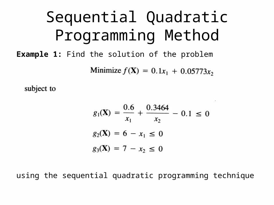
Example 1: Find the solution of the problem
using the sequential quadratic programming technique
Sequential Quadratic Programming Method - Example 1
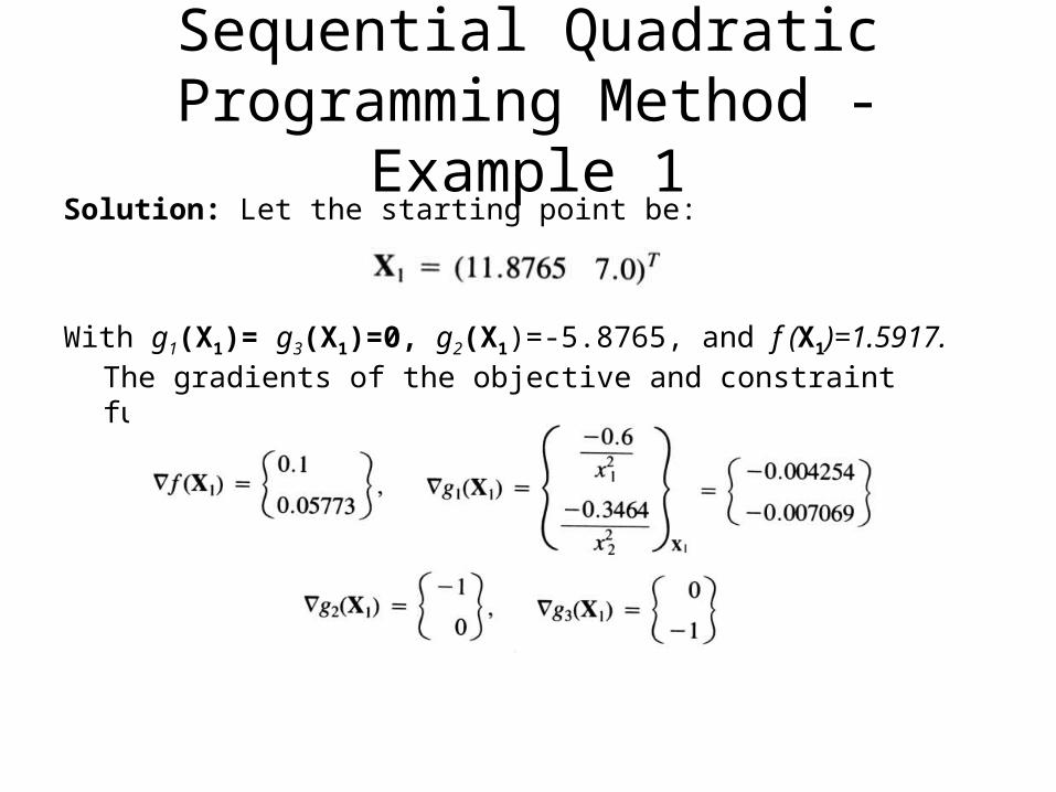
Solution: Let the starting point be:
With g1(X1)= g3(X1)=0, g2(X1)=-5.8765, and f (X1)=1.5917. The gradients of the objective and constraint functions at X1 are given by:
Sequential Quadratic Programming Method - Example 1
Solution:
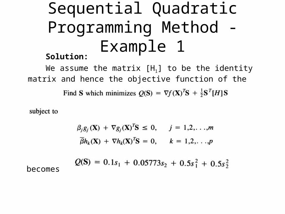
We assume the matrix [H1] to be the identity matrix and hence the objective function of the equation
becomes
Sequential Quadratic Programming Method - Example 1
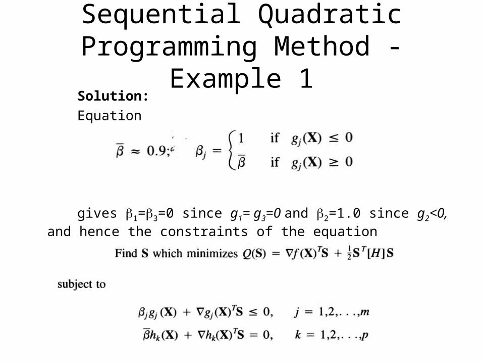
Solution:
Equation
gives 1=3=0 since g1= g3=0 and 2=1.0 since g2<0, and hence the constraints of the equation
Sequential Quadratic Programming Method - Example 1
Solution:
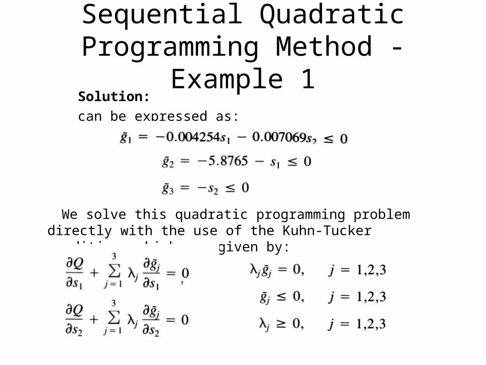
can be expressed as:
We solve this quadratic programming problem directly with the use of the Kuhn-Tucker conditions which are given by:
Sequential Quadratic Programming Method - Example 1
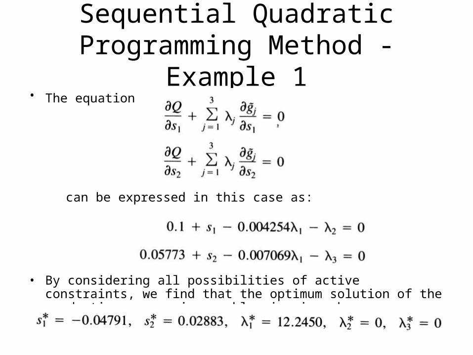
• The equations
can be expressed in this case as:
• By considering all possibilities of active constraints, we find that the optimum solution of the quadratic programming problem is given by
Sequential Quadratic Programming Method - Example 1
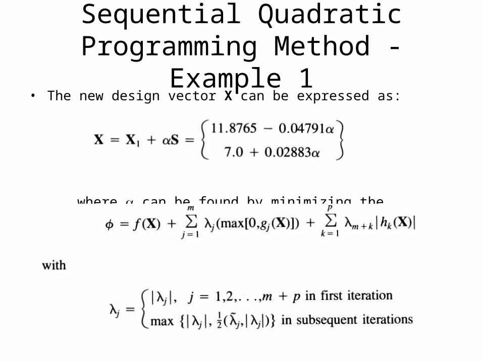
• The new design vector X can be expressed as:
where can be found by minimizing the function in equation
Sequential Quadratic Programming Method - Example 1
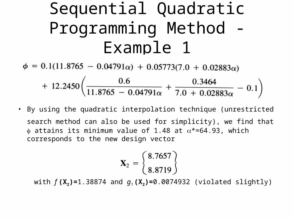
• By using the quadratic interpolation technique (unrestricted search method
can also be used for simplicity), we find that attains its minimum value of 1.48 at *=64.93, which corresponds to the new design vector
with f (X2)=1.38874 and g1 (X2)=0.0074932 (violated slightly)
Sequential Quadratic Programming Method - Example 1
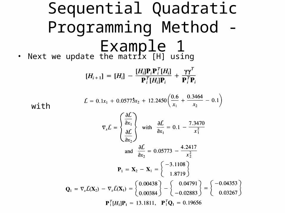
• Next we update the matrix [H] using
with
Sequential Quadratic Programming Method - Example 1
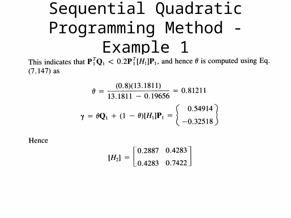
Sequential Quadratic Programming Method - Example 1
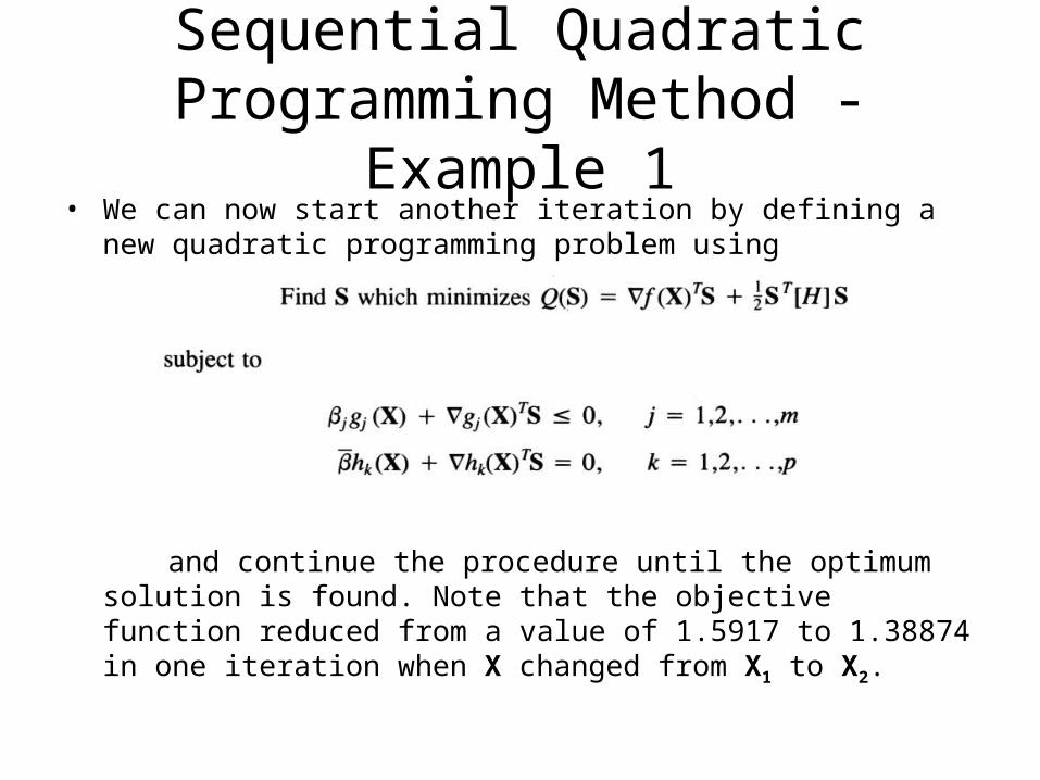
• We can now start another iteration by defining a new quadratic programming problem using
and continue the procedure until the optimum solution is found. Note that the objective function reduced from a value of 1.5917 to 1.38874 in one iteration when X changed from X1 to X2.
Indirect methods
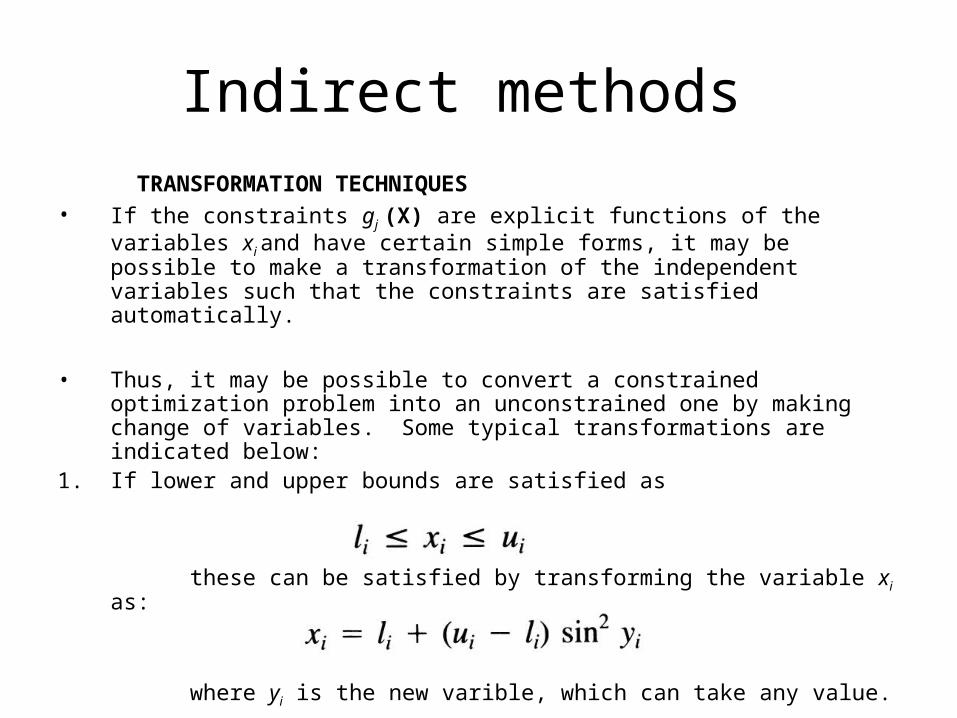
TRANSFORMATION TECHNIQUES• If the constraints gj (X) are explicit functions of the variables xi and have
certain simple forms, it may be possible to make a transformation of the independent variables such that the constraints are satisfied automatically.
• Thus, it may be possible to convert a constrained optimization problem into an unconstrained one by making change of variables. Some typical transformations are indicated below:
1. If lower and upper bounds are satisfied as
these can be satisfied by transforming the variable xi as:
where yi is the new varible, which can take any value.
Indirect methods
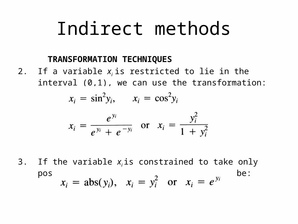
TRANSFORMATION TECHNIQUES
2. If a variable xi is restricted to lie in the interval (0,1), we can use the transformation:
3. If the variable xi is constrained to take only positive values, the transformation can be:
Indirect methods
TRANSFORMATION TECHNIQUES
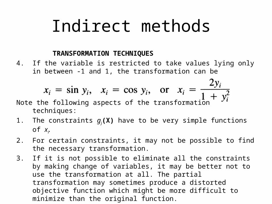
4. If the variable is restricted to take values lying only in between -1 and 1, the transformation can be
Note the following aspects of the transformation techniques:
1. The constraints gj(X) have to be very simple functions of xi.
2. For certain constraints, it may not be possible to find the necessary transformation.
3. If it is not possible to eliminate all the constraints by making change of variables, it may be better not to use the transformation at all. The partial transformation may sometimes produce a distorted objective function which might be more difficult to minimize than the original function.
Indirect methods-Example 1
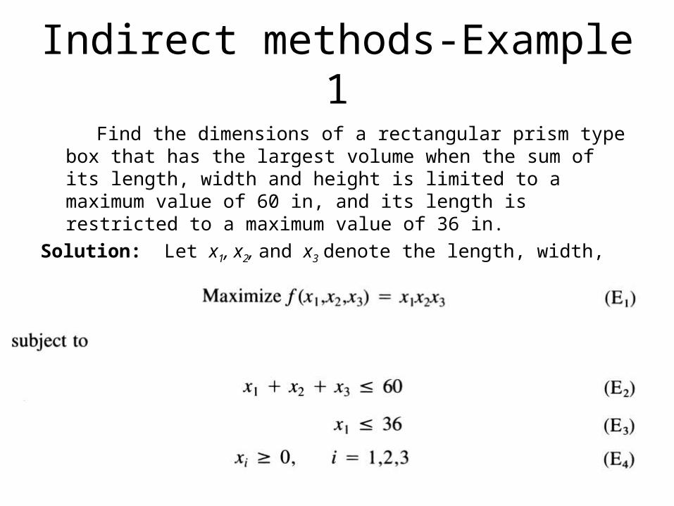
Find the dimensions of a rectangular prism type box that has the largest volume when the sum of its length, width and height is limited to a maximum value of 60 in, and its length is restricted to a maximum value of 36 in.
Solution: Let x1, x2, and x3 denote the length, width, and height of the box, respectively. The problem can be stated as follows:
Indirect methods-Example 1
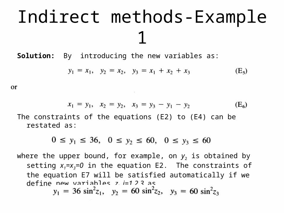
Solution: By introducing the new variables as:
The constraints of the equations (E2) to (E4) can be restated as:
where the upper bound, for example, on y2 is obtained by setting x1=x3=0 in the equation E2. The constraints of the equation E7 will be satisfied automatically if we define new variables zi, i=1,2,3, as
Indirect methods-Example 1
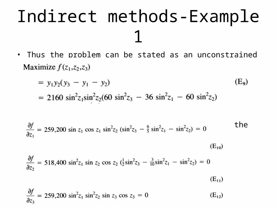
• Thus the problem can be stated as an unconstrained problem as follows:
• The necessary conditions of optimality yield the relations:
• Equation E12 gives the nontrivial solution as cos z3=0 or sin2z3=1. Hence the equations E10 and E11 yield sin2z1=5/9 and sin2z2=1/3.
• Thus the optimal solution is given by x1*=20 in., x2*=20 in., x3*=20 in., and the maximum volume =8000 in3.
BASIC APPROACH OF THE PENALTY FUNCTION METHOD
• Penalty function methods transform the basic optimization problem into alternative formulations such that numerical solutions are sought by solving a sequence of unconstrained minimization problems.
Indirect methods
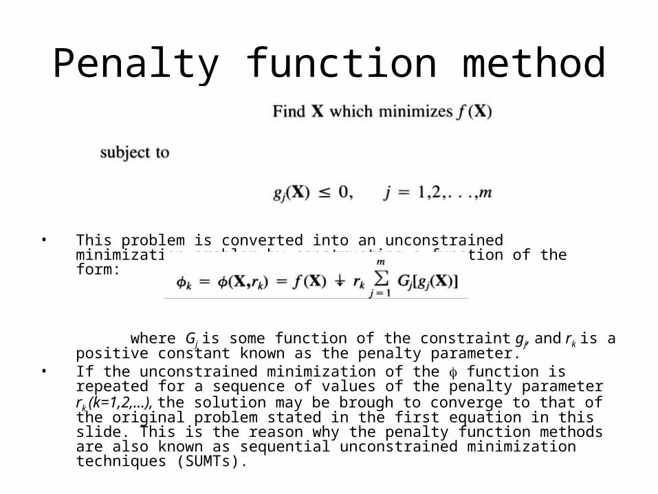
• This problem is converted into an unconstrained minimization problem by constructing a function of the form:
where Gj is some function of the constraint gj, and rk is a positive constant known as the penalty parameter.
• If the unconstrained minimization of the function is repeated for a sequence of values of the penalty parameter rk (k=1,2,...), the solution may be brough to converge to that of the original problem stated in the first equation in this slide. This is the reason why the penalty function methods are also known as sequential unconstrained minimization techniques (SUMTs).
Penalty function method
Penalty function method
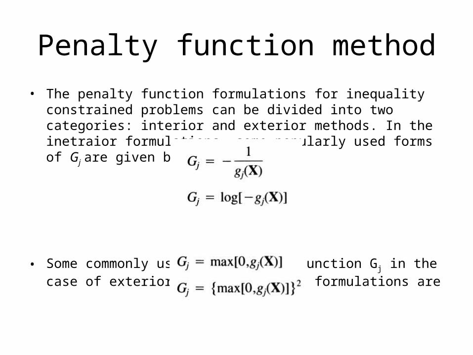
• The penalty function formulations for inequality constrained problems can be divided into two categories: interior and exterior methods. In the inetraior formulations, some popularly used forms of Gj are given by:
• Some commonly used forms of the function Gj in the case of exterior penalty function formulations are
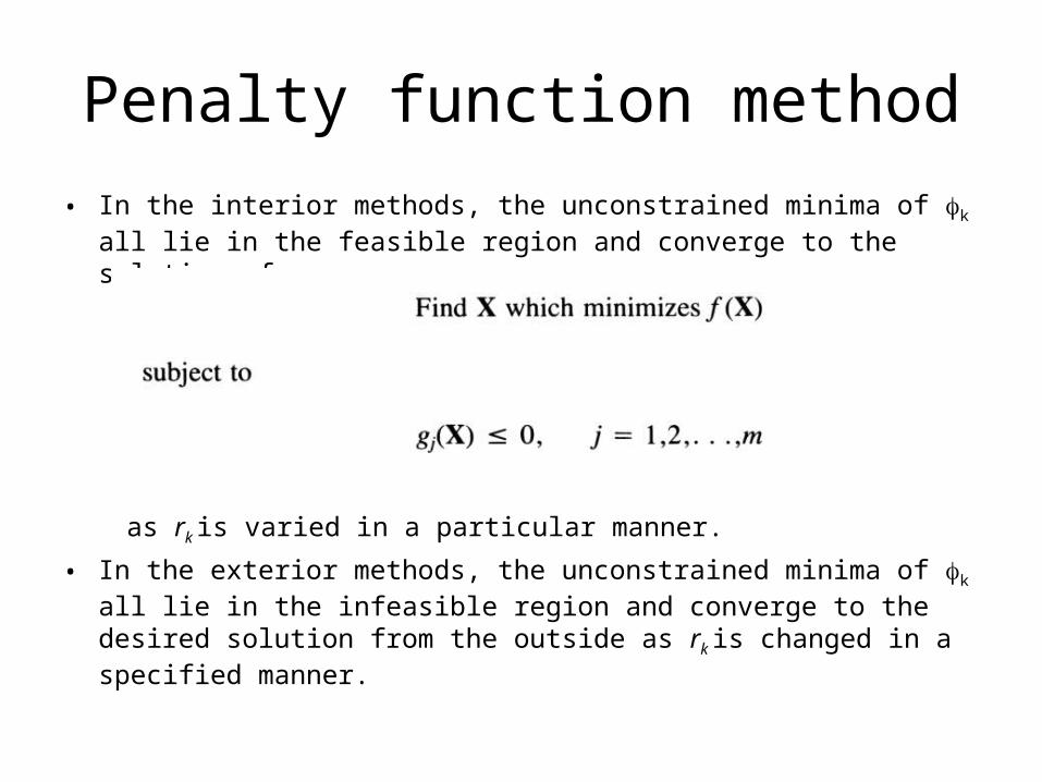
• In the interior methods, the unconstrained minima of k all lie in the feasible region and converge to the solution of
as rk is varied in a particular manner.
• In the exterior methods, the unconstrained minima of k all lie in the infeasible region and converge to the desired solution from the outside as rk
is changed in a specified manner.
Penalty function method
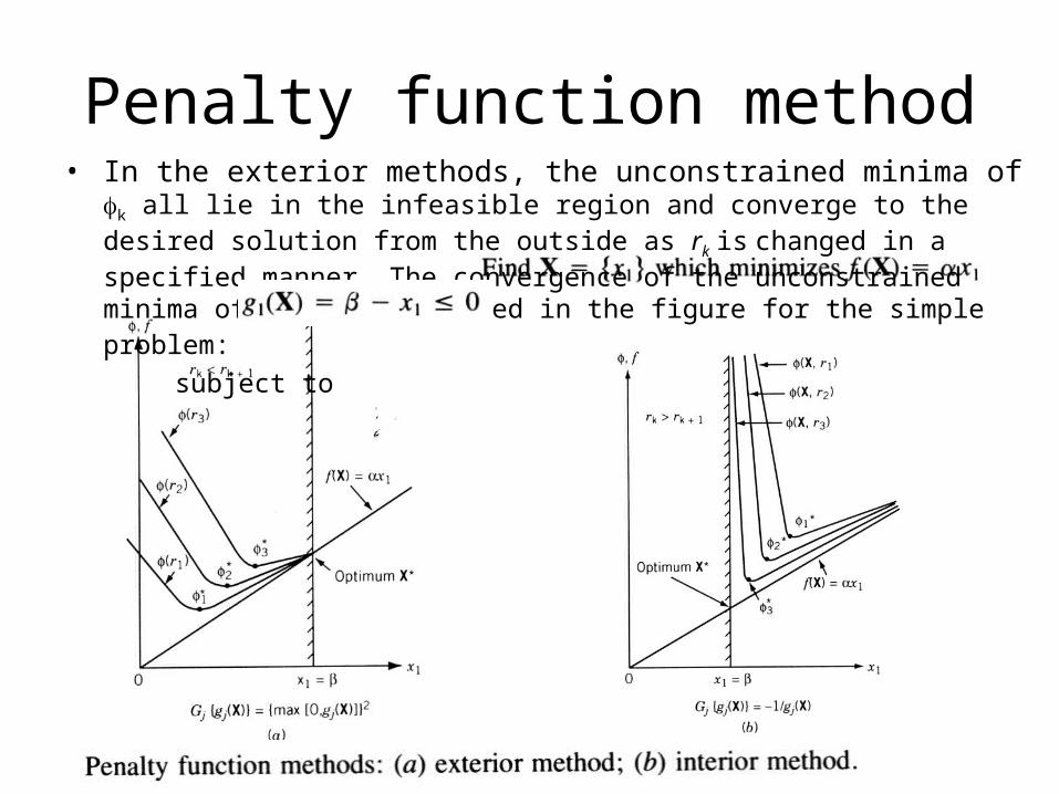
• In the exterior methods, the unconstrained minima of k all lie in the infeasible region and converge to the desired solution from the outside as rk is changed in a specified manner. The convergence of the unconstrained minima of k is illustrated in the figure for the simple problem:
subject to
Penalty function method
Penalty function method
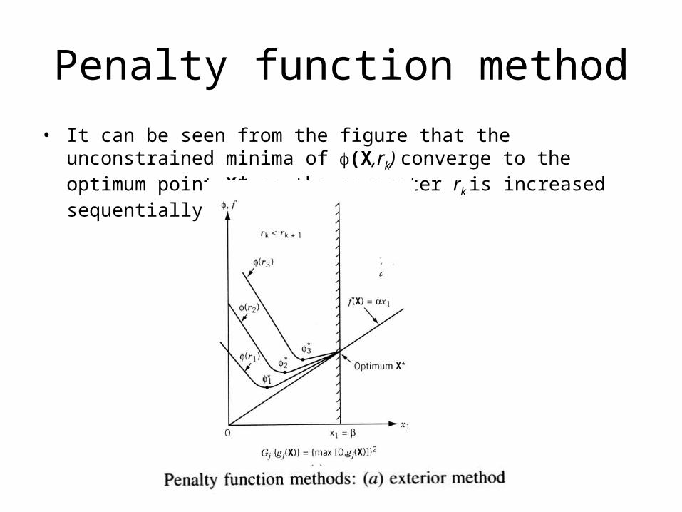
• It can be seen from the figure that the unconstrained minima of (X,rk) converge to the optimum point X* as the parameter rk is increased sequentially.
Penalty function method
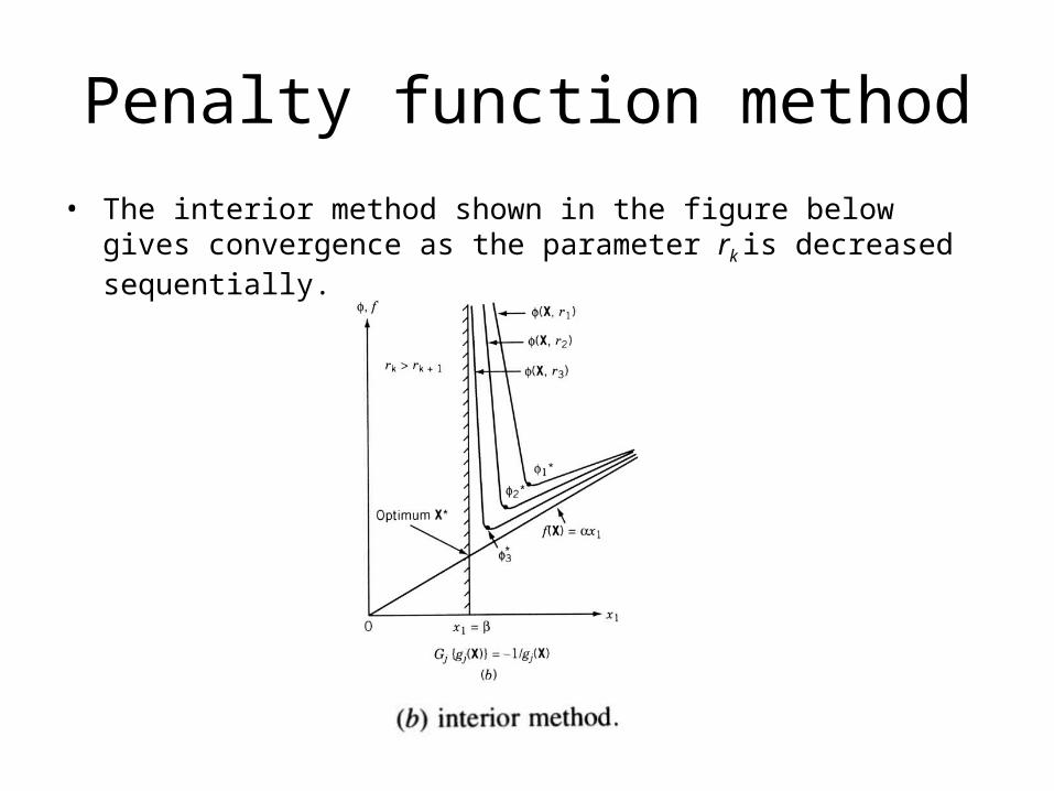
• The interior method shown in the figure below gives convergence as the parameter rk is decreased sequentially.
Penalty function method
• There are several reasons for the appeal of the penalty function formulations. One main reason, which can be observed from the figures in the previous slides is that the sequential nature of the method allows a gradual or sequential approach to criticality of the constraints.
• In addition, the sequential process permits a graded approximation to be used in the analysis of the system. This means that if the evaluation of f and gj [and hence (X,rk) ] for any specified design vector X is computationally very difficult, we can use coarse approximations during the early stages of optimization (when the unconstrained minima of k are far away from the optimum) and finer or more detailed analysis approximation during the final stages of optimization.
Interior Penalty Function Method
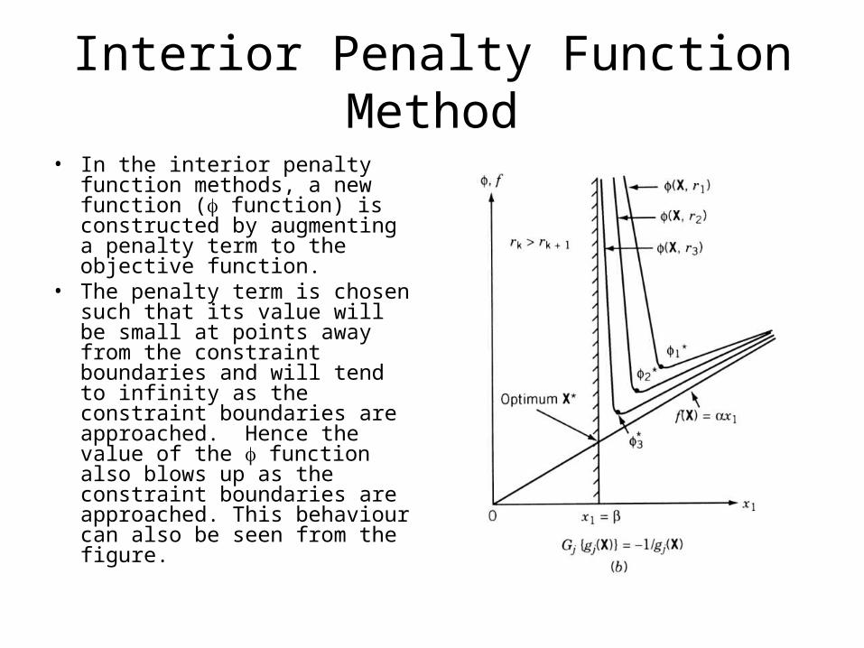
• In the interior penalty function methods, a new function ( function) is constructed by augmenting a penalty term to the objective function.
• The penalty term is chosen such that its value will be small at points away from the constraint boundaries and will tend to infinity as the constraint boundaries are approached. Hence the value of the function also blows up as the constraint boundaries are approached. This behaviour can also be seen from the figure.
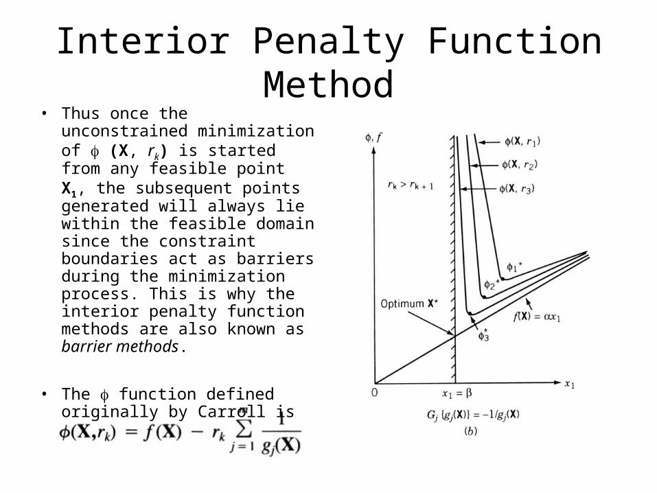
Interior Penalty Function Method• Thus once the unconstrained
minimization of (X, rk) is started from any feasible point X1, the subsequent points generated will always lie within the feasible domain since the constraint boundaries act as barriers during the minimization process. This is why the interior penalty function methods are also known as barrier methods.
• The function defined originally by Carroll is
Interior Penalty Function Method
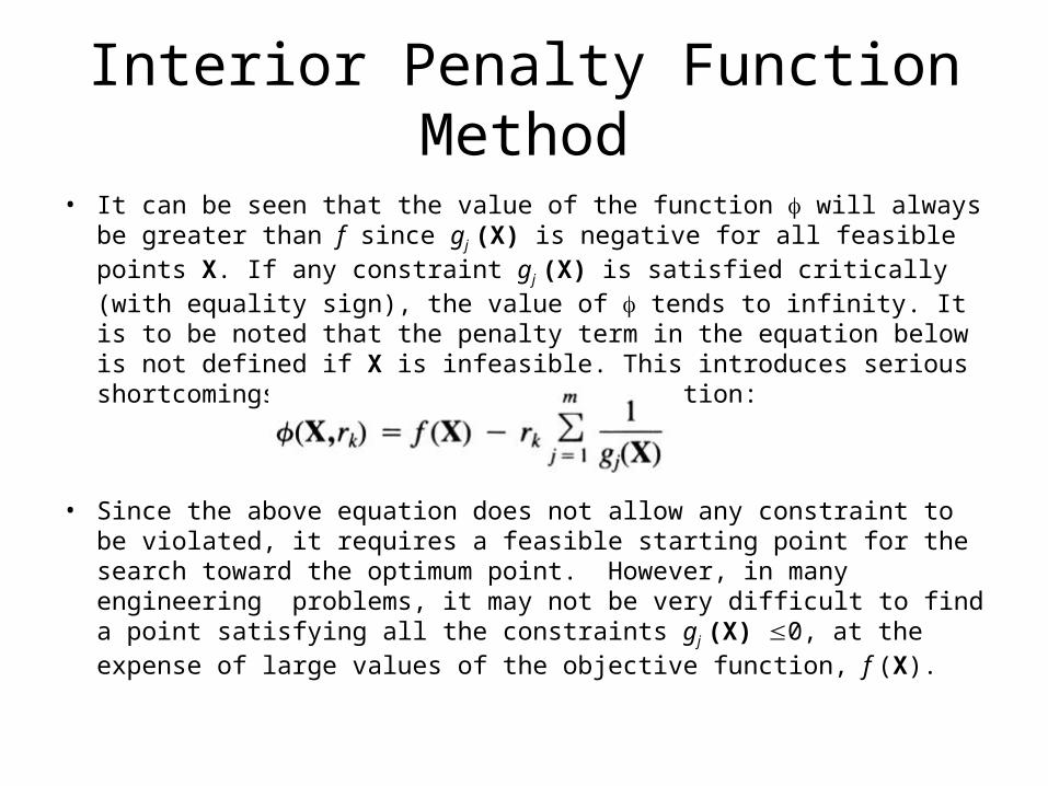
• It can be seen that the value of the function will always be greater than f since gj (X) is negative for all feasible points X. If any constraint gj (X) is satisfied critically (with equality sign), the value of tends to infinity. It is to be noted that the penalty term in the equation below is not defined if X is infeasible. This introduces serious shortcomings while using the below equation:
• Since the above equation does not allow any constraint to be violated, it requires a feasible starting point for the search toward the optimum point. However, in many engineering problems, it may not be very difficult to find a point satisfying all the constraints gj (X) 0, at the expense of large values of the objective function, f (X).
Interior Penalty Function Method
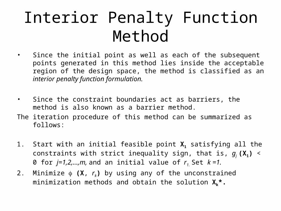
• Since the initial point as well as each of the subsequent points generated in this method lies inside the acceptable region of the design space, the method is classified as an interior penalty function formulation.
• Since the constraint boundaries act as barriers, the method is also known as a barrier method.
The iteration procedure of this method can be summarized as follows:
1. Start with an initial feasible point X1 satisfying all the constraints with strict inequality sign, that is, gj (X1) < 0 for j=1,2,...,m, and an initial value of r1. Set k =1.
2. Minimize (X, rk) by using any of the unconstrained minimization methods and obtain the solution Xk*.
Interior Penalty Function Method
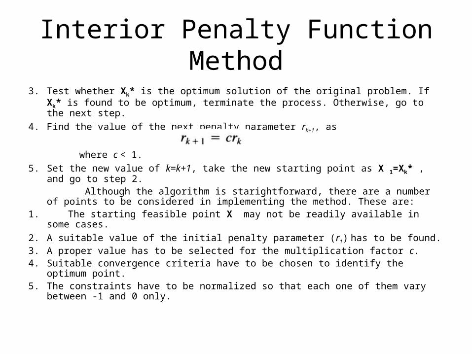
3. Test whether Xk* is the optimum solution of the original problem. If Xk* is found to be optimum, terminate the process. Otherwise, go to the next step.
4. Find the value of the next penalty parameter rk+1, as
where c < 1.
5. Set the new value of k=k+1, take the new starting point as X 1=Xk* , and go to step 2.
Although the algorithm is starightforward, there are a number of points to be considered in implementing the method. These are:
1. The starting feasible point X may not be readily available in some cases.
2. A suitable value of the initial penalty parameter (r1) has to be found.3. A proper value has to be selected for the multiplication factor c.4. Suitable convergence criteria have to be chosen to identify the optimum point.5. The constraints have to be normalized so that each one of them vary between -1
and 0 only.
Starting Feasible Point X1
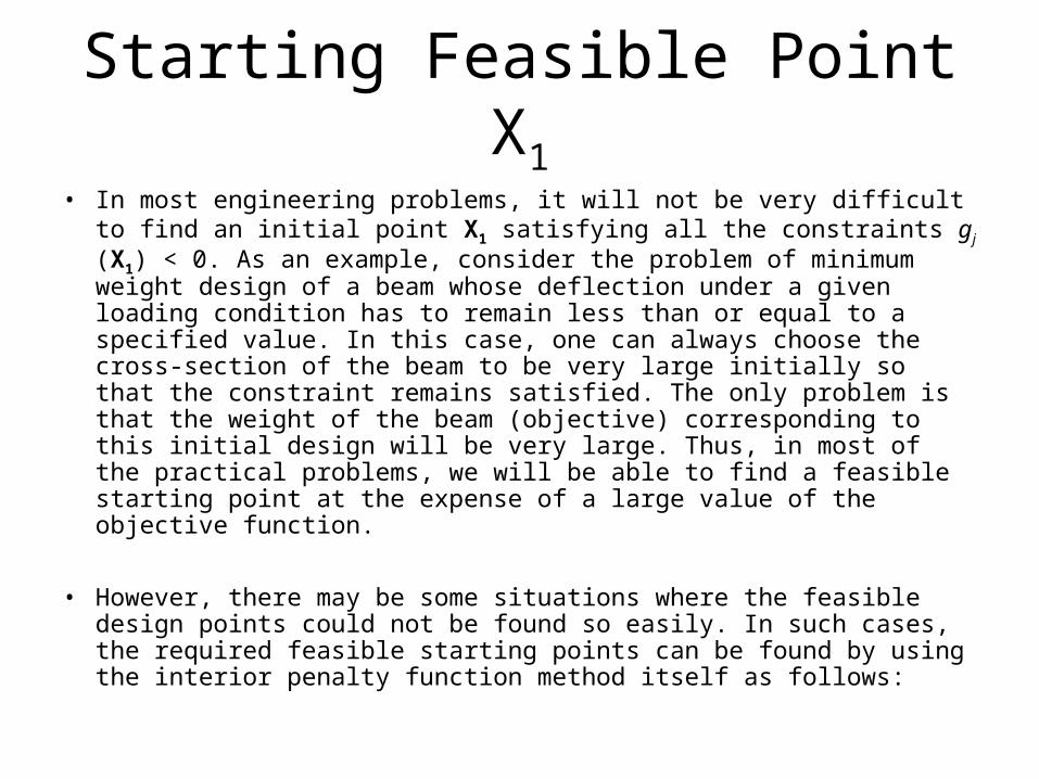
• In most engineering problems, it will not be very difficult to find an initial point X1 satisfying all the constraints gj (X1) < 0. As an example, consider the problem of minimum weight design of a beam whose deflection under a given loading condition has to remain less than or equal to a specified value. In this case, one can always choose the cross-section of the beam to be very large initially so that the constraint remains satisfied. The only problem is that the weight of the beam (objective) corresponding to this initial design will be very large. Thus, in most of the practical problems, we will be able to find a feasible starting point at the expense of a large value of the objective function.
• However, there may be some situations where the feasible design points could not be found so easily. In such cases, the required feasible starting points can be found by using the interior penalty function method itself as follows:

Starting Feasible Point X1
1. Choose an arbitrary point X1 and evaluate the constraints gj (X) at the point X1. Since the point X1 is arbitrary, it may not satisfy all the constraints with strict inequality sign. If r out of the total of m constraints are violated, renumber the constraints such that the last r constraints will become the violated ones, that is,
2. Identify the constraint that is violated most at the point X1, that is, find the integer k such that
Starting Feasible Point X1
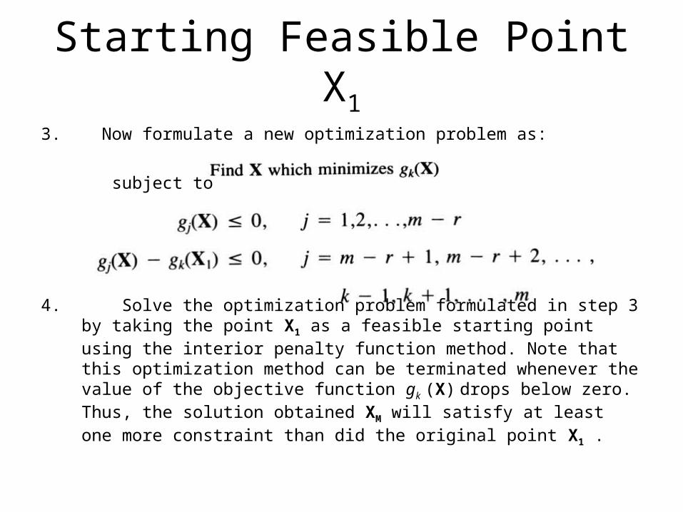
3. Now formulate a new optimization problem as:
subject to
4. Solve the optimization problem formulated in step 3 by taking the point X1 as a feasible starting point using the interior penalty function method. Note that this optimization method can be terminated whenever the value of the objective function gk (X) drops below zero. Thus, the solution obtained XM will satisfy at least one more constraint than did the original point X1 .
Starting Feasible Point X1
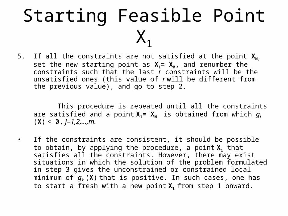
5. If all the constraints are not satisfied at the point XM, set the new starting point as X1= XM, and renumber the constraints such that the last r constraints will be the unsatisfied ones (this value of r will be different from the previous value), and go to step 2.
This procedure is repeated until all the constraints are satisfied and a point X1= XM is obtained from which gj (X) < 0, j=1,2,...,m.
• If the constraints are consistent, it should be possible to obtain, by applying the procedure, a point X1 that satisfies all the constraints. However, there may exist situations in which the solution of the problem formulated in step 3 gives the unconstrained or constrained local minimum of gk (X) that is positive. In such cases, one has to start a fresh with a new point X1 from step 1 onward.
Initial value of the penalty parameter r1
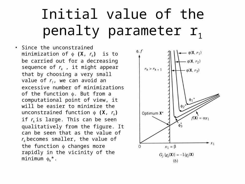
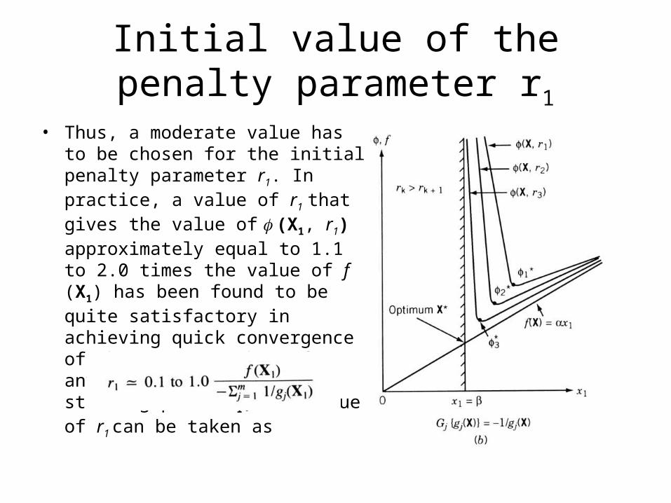
• Since the unconstrained minimization of (X, rk) is to be carried out for a decreasing sequence of rk , it might appear that by choosing a very small value of r1, we can avoid an excessive number of minimizations of the function . But from a computational point of view, it will be easier to minimize the unconstrained function (X, rk) if rk is large. This can be seen qualitatively from the figure. It can be seen that as the value of rk becomes smaller, the value of the function changes more rapidly in the vicinity of the minimum k*.
Initial value of the penalty parameter r1
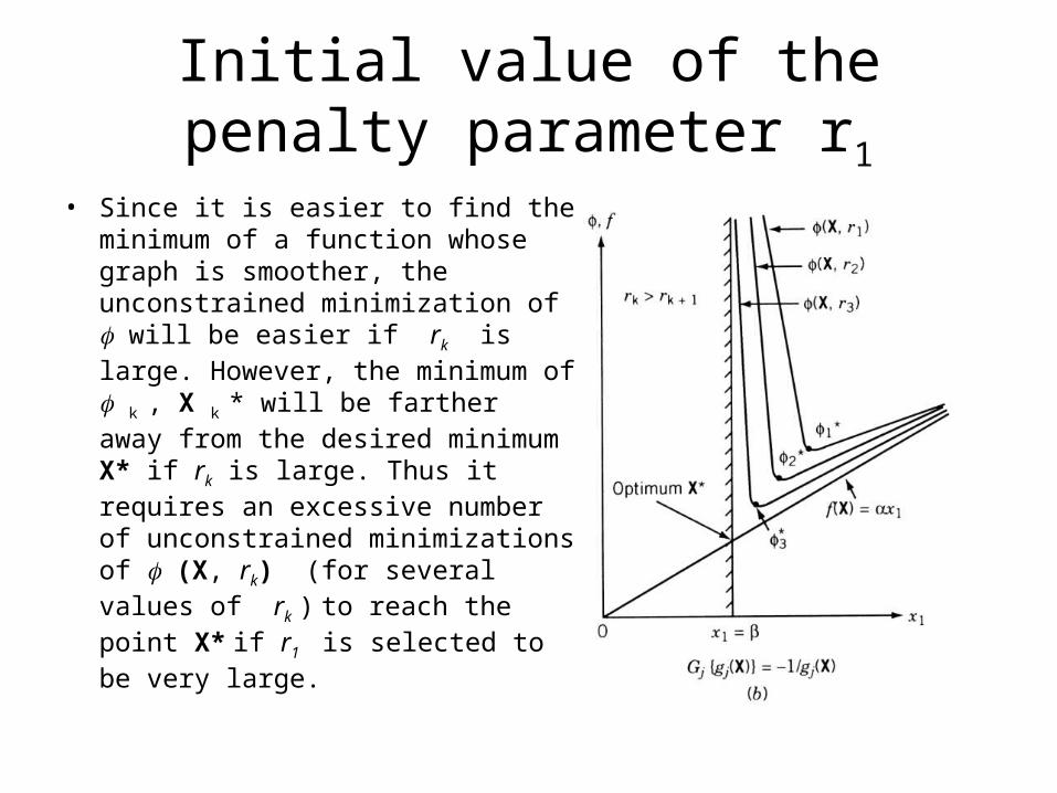
• Since it is easier to find the minimum of a function whose graph is smoother, the unconstrained minimization of will be easier if rk is large. However, the minimum of k , X k * will be farther away from the desired minimum X* if rk is large. Thus it requires an excessive number of unconstrained minimizations of (X, rk) (for several values of rk ) to reach the point X* if r1 is selected to be very large.
Initial value of the penalty parameter r1
• Thus, a moderate value has to be chosen for the initial penalty parameter r1. In practice, a value of r1 that gives the value of (X1, r1) approximately equal to 1.1 to 2.0 times the value of f (X1) has been found to be quite satisfactory in achieving quick convergence of the process. Thus, for any initial feasible starting point X1, the value of r1 can be taken as
Subsequent values of the penalty parameter
• Once the initial value of rk is chosen, the subsequent values of rk have to be chosen such that
For convenience, the values of rk are chosen according to the relation
where c<1. The value of c can be taken as 0.1, 0.2 or 0.5.
Convergence Criteria
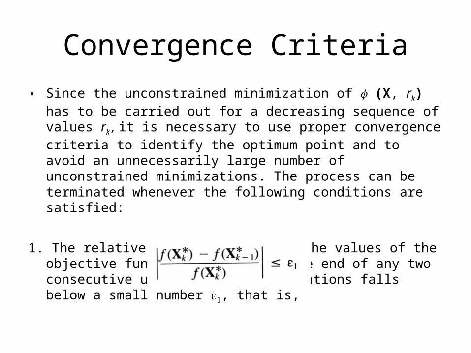
• Since the unconstrained minimization of (X, rk) has to be carried out for a decreasing sequence of values rk , it is necessary to use proper convergence criteria to identify the optimum point and to avoid an unnecessarily large number of unconstrained minimizations. The process can be terminated whenever the following conditions are satisfied:
1. The relative difference between the values of the objective function obtained at the end of any two consecutive unconstrained minimizations falls below a small number 1, that is,
Convergence Criteria
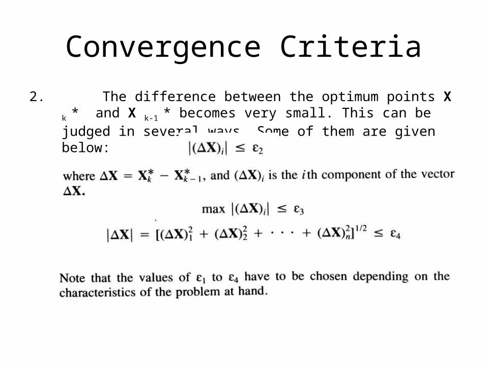
2. The difference between the optimum points X k * and X k-1 * becomes very small. This can be judged in several ways. Some of them are given below:
Normalization of Constraints
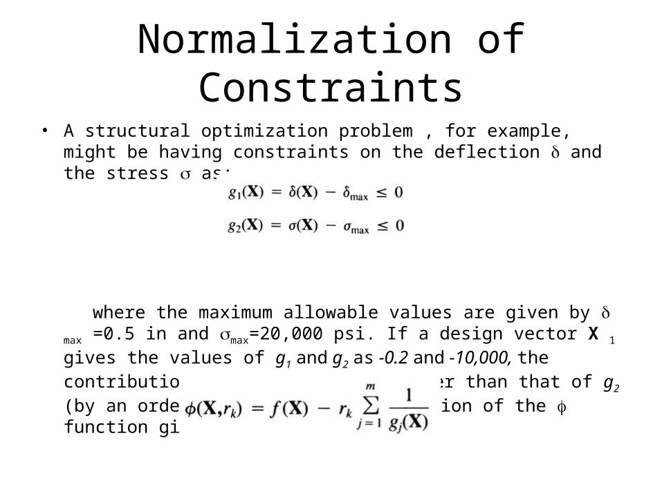
• A structural optimization problem , for example, might be having constraints on the deflection and the stress as:
where the maximum allowable values are given by max =0.5 in and max=20,000 psi. If a design vector X 1 gives the values of g1 and g2 as -0.2 and -10,000, the contribution of g1 will be much larger than that of g2 (by an order of 104) in the formulation of the function given by the equation
Normalization of Constraints
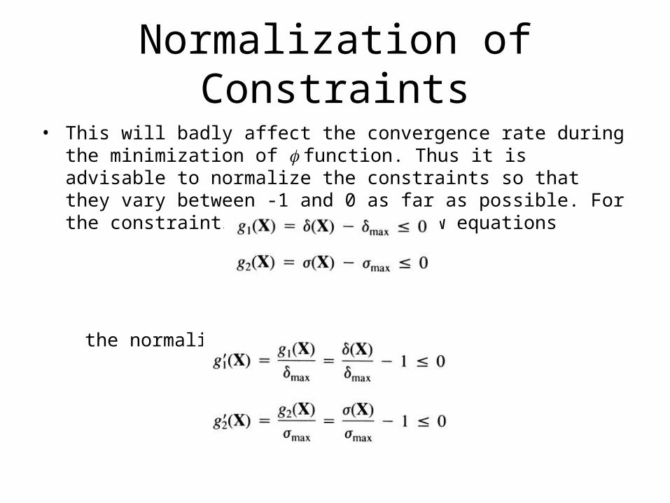
• This will badly affect the convergence rate during the minimization of function. Thus it is advisable to normalize the constraints so that they vary between -1 and 0 as far as possible. For the constraints shown in the below equations
the normalization can be done as:
Normalization of Constraints
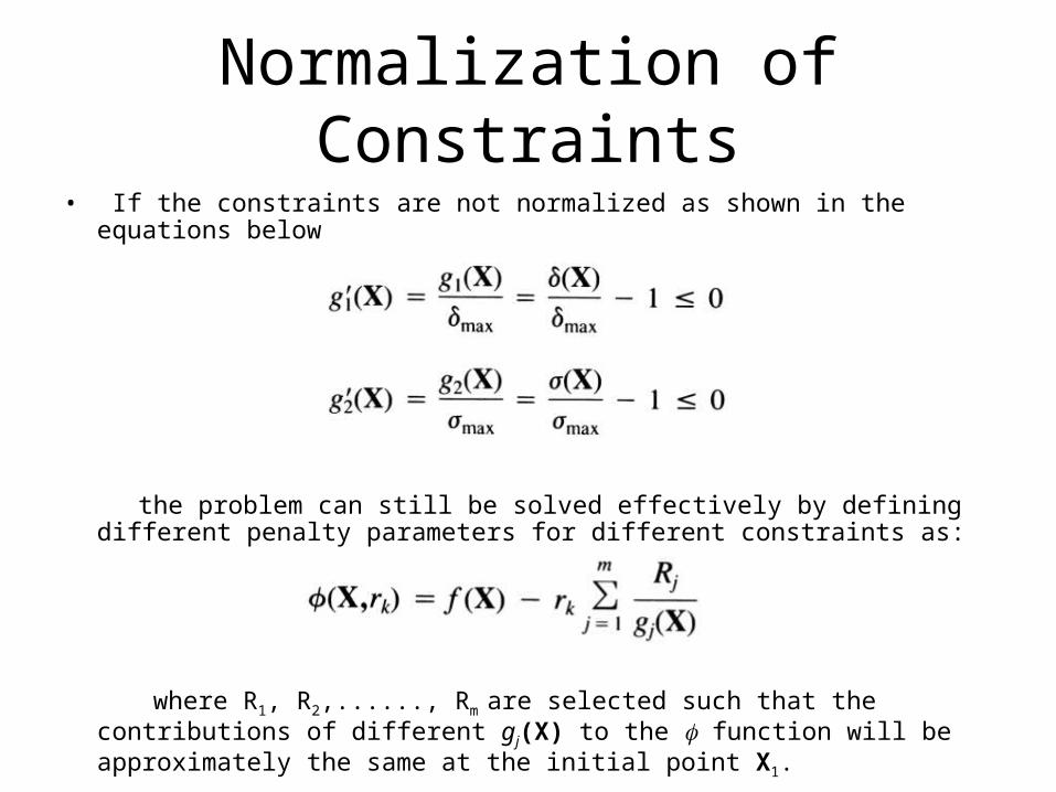
• If the constraints are not normalized as shown in the equations below
the problem can still be solved effectively by defining different penalty parameters for different constraints as:
where R1, R2,......, Rm are selected such that the contributions of different gj(X) to the function will be approximately the same at the initial point X1.
Normalization of Constraints
• When the unconstrained minimization of (X, rk) is carried for a decreasing sequence of values of rk , the values of R1, R2,......, Rm will not be altered; however, they are expected to be effective in reducing the disparities between the contributions of the various constraints to the function.
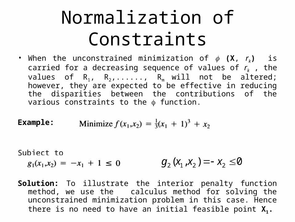
Example:
Subject to
Solution: To illustrate the interior penalty function method, we use the
calculus method for solving the unconstrained minimization problem in this case. Hence there is no need to have an initial feasible point X1.
0),( 2212 xxxg
Example 1
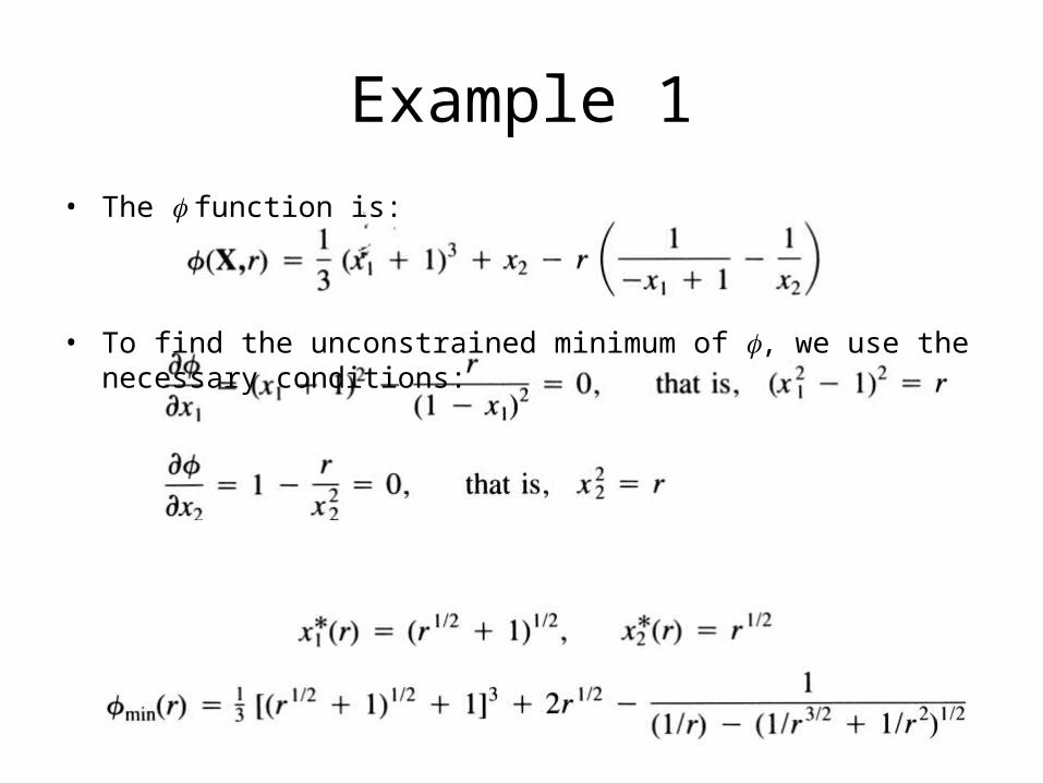
• The function is:
• To find the unconstrained minimum of , we use the necessary conditions:
• These equations give:
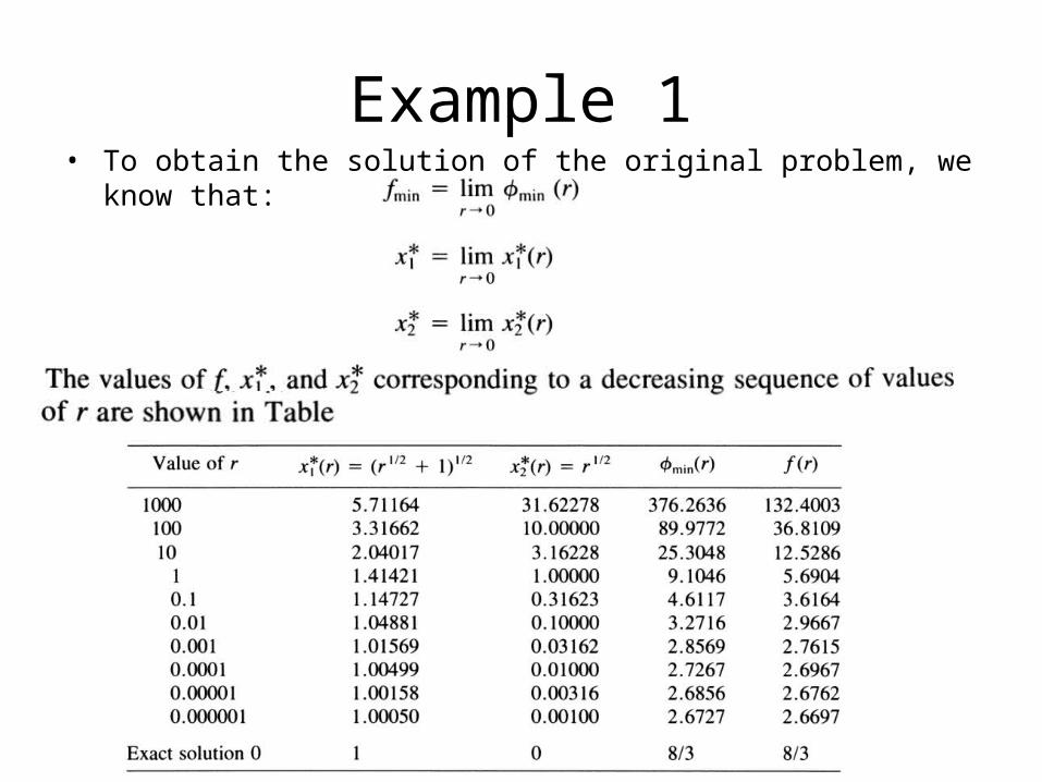
Example 1• To obtain the solution of the original problem, we know that:
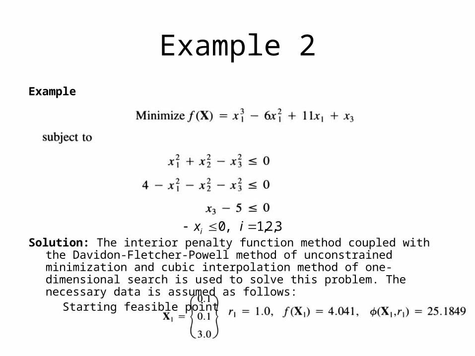
Example 2Example
Solution: The interior penalty function method coupled with the Davidon-Fletcher-
Powell method of unconstrained minimization and cubic interpolation method of one-dimensional search is used to solve this problem. The necessary data is assumed as follows:
Starting feasible point:
3,2,1,0 ixi
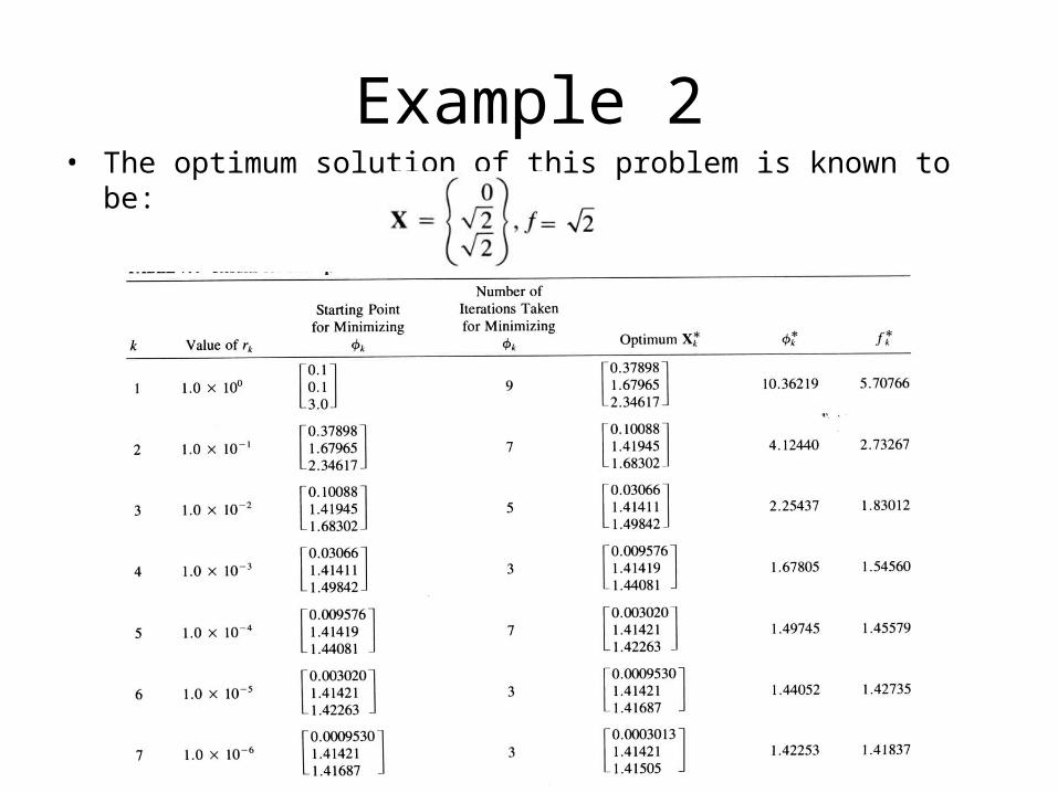
• The optimum solution of this problem is known to be:
Example 2
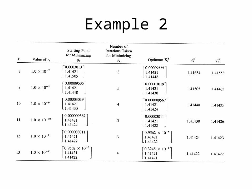
Example 2
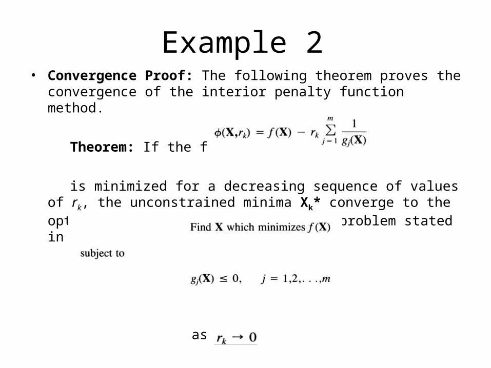
• Convergence Proof: The following theorem proves the convergence of the interior penalty function method.
Theorem: If the function
is minimized for a decreasing sequence of values of rk, the unconstrained minima Xk* converge to the optimum solution of the constrained problem stated in
as
Example 2
Convex Programming Problem
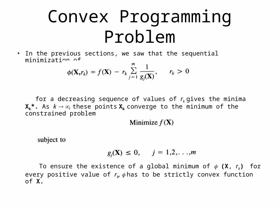
• In the previous sections, we saw that the sequential minimization of
for a decreasing sequence of values of rk gives the minima Xk*. As k , these points Xk converge to the minimum of the constrained problem
To ensure the existence of a global minimum of (X, rk) for every positive value of rk, has to be strictly convex function of X.
Convex Programming Problem
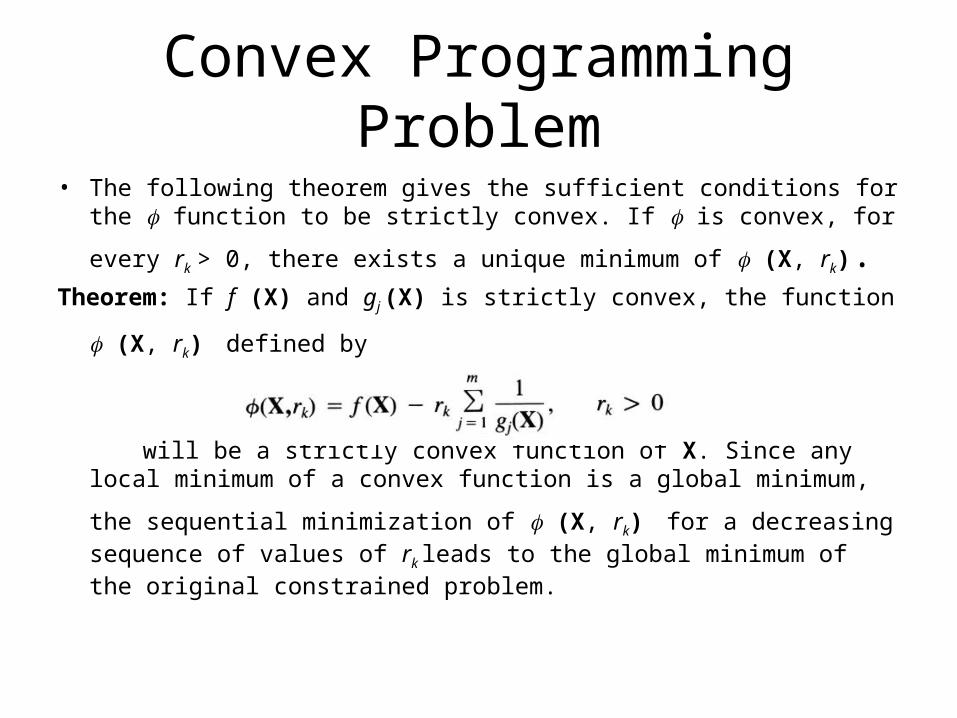
• The following theorem gives the sufficient conditions for the function to be strictly convex. If is convex, for every rk > 0, there exists a unique
minimum of (X, rk).
Theorem: If f (X) and gj (X) is strictly convex, the function (X, rk) defined by
will be a strictly convex function of X. Since any local minimum of a convex function is a global minimum, the sequential minimization of (X,
rk) for a decreasing sequence of values of rk leads to the global minimum of the original constrained problem.
Convex Programming Problem
• When the convexity conditions are not satisfied, or when the functions are so complex that we do not know beforehand whether the convexity conditions are satisfied, it will not be possible to prove that the minimum found by the SUMT method is a global one. In such cases, one has to satisfy with a local minimum only.
• However, one can always reapply the SUMT method from different feasible starting points and try to find a better local minimum point if the problem has several local minima. Of course, this procedure requires more computational effort.
Exterior Penalty Function Method
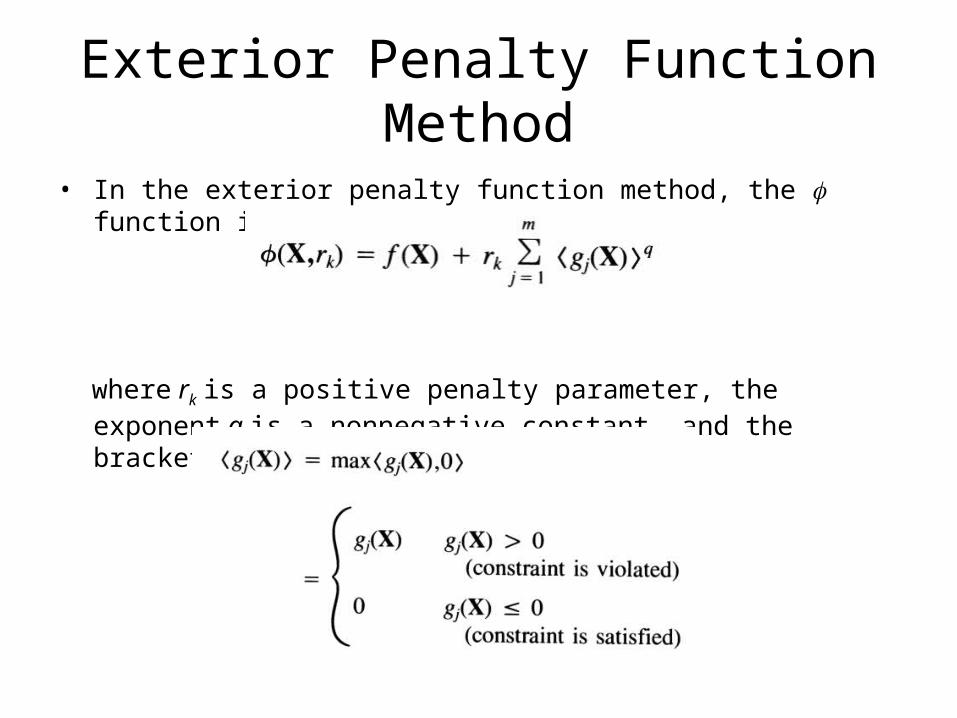
• In the exterior penalty function method, the function is generally taken as:
where rk is a positive penalty parameter, the exponent q is a nonnegative constant, and the bracket function gj(X) is defined as:
Exterior Penalty Function Method
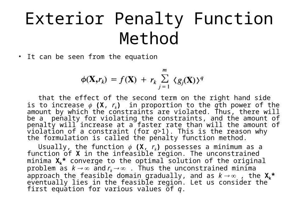
• It can be seen from the equation
that the effect of the second term on the right hand side is to increase (X, rk) in proportion to the qth power of the amount by which the constraints are violated. Thus, there will be a penalty for violating the constraints, and the amount of penalty will increase at a faster rate than will the amount of violation of a constraint (for q>1). This is the reason why the formulation is called the penalty function method.
Usually, the function (X, rk) possesses a minimum as a function of X in the infeasible region. The unconstrained minima Xk* converge to the optimal solution of the original problem as k and rk . Thus the unconstrained minima approach the feasible domain gradually, and as k , the Xk* eventually lies in the feasible region. Let us consider the first equation for various values of q.
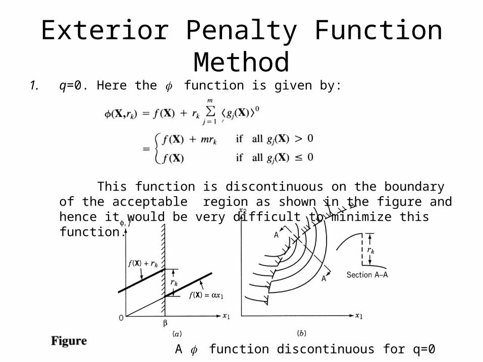
Exterior Penalty Function Method1. q=0. Here the function is given by:
This function is discontinuous on the boundary of the acceptable region as shown in the figure and hence it would be very difficult to minimize this function.
A function discontinuous for q=0
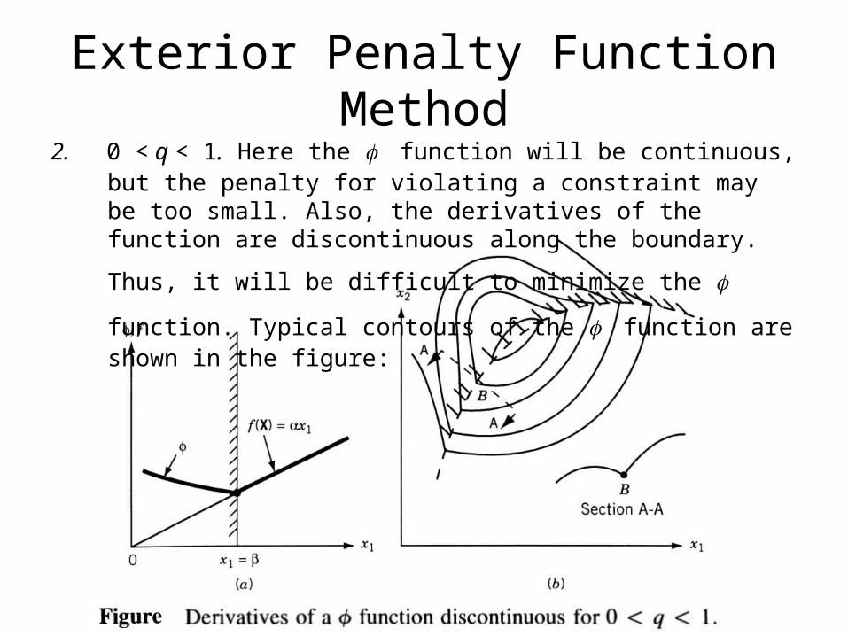
Exterior Penalty Function Method2. 0 < q < 1. Here the function will be continuous, but the penalty for
violating a constraint may be too small. Also, the derivatives of the function are discontinuous along the boundary. Thus, it will be difficult
to minimize the function. Typical contours of the function are shown in the figure:
Exterior Penalty Function Method
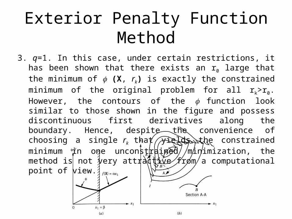
3. q=1. In this case, under certain restrictions, it has been shown that there exists an r0 large that the minimum of (X, rk) is exactly the constrained minimum of the original problem for all rk>r0. However, the contours of the function look similar to those shown in the figure and possess discontinuous first derivatives along the boundary. Hence, despite the convenience of choosing a single rk that yields the constrained minimum in one unconstrained minimization, the method is not very attractive from a computational point of view.
Exterior Penalty Function Method
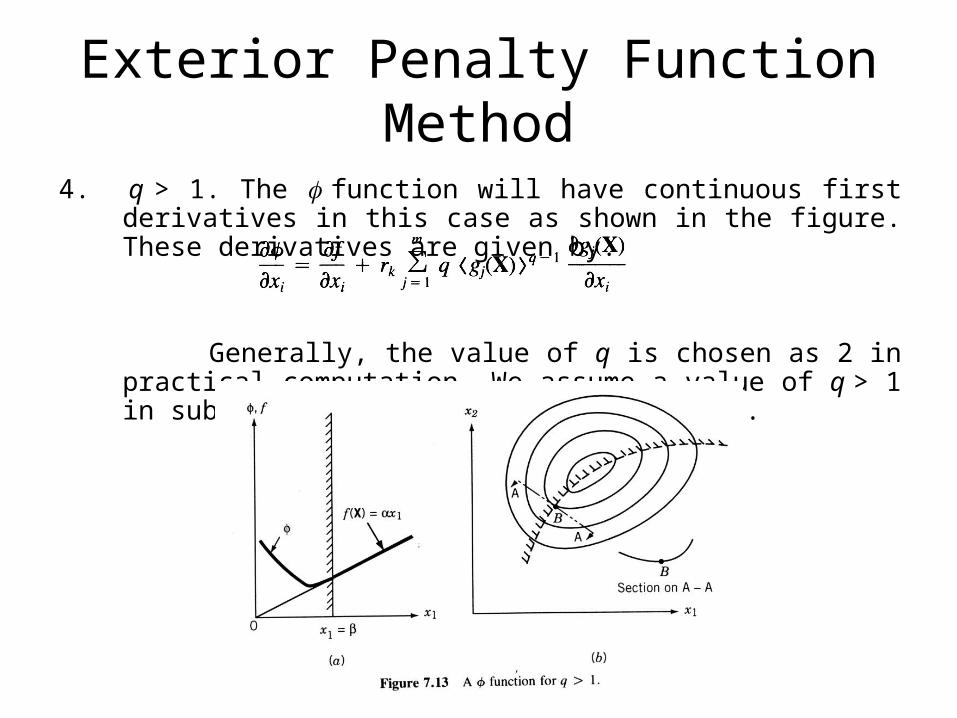
4. q > 1. The function will have continuous first derivatives in this case as shown in the figure. These derivatives are given by:
Generally, the value of q is chosen as 2 in practical computation. We assume a value of q > 1 in subsequent discussion of this method.
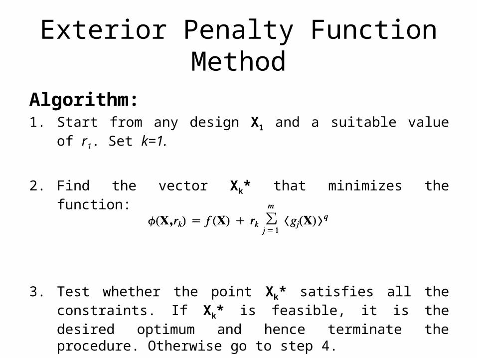
Algorithm:1. Start from any design X1 and a suitable value of r1. Set k=1.
2. Find the vector Xk* that minimizes the function:
3. Test whether the point Xk* satisfies all the constraints. If Xk* is feasible, it is the desired optimum and hence terminate the procedure. Otherwise go to step 4.
Exterior Penalty Function Method
Exterior Penalty Function Method
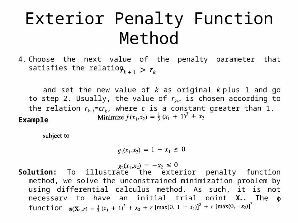
4. Choose the next value of the penalty parameter that satisfies the relation
and set the new value of k as original k plus 1 and go to step 2. Usually, the value of rk+1 is chosen according to the relation rk+1=crk, where c is a constant greater than 1.
Example
Solution: To illustrate the exterior penalty function method, we solve the unconstrained minimization problem by using differential calculus method. As such, it is not necessary to have an initial trial point X1. The function is
Exterior Penalty Function Method
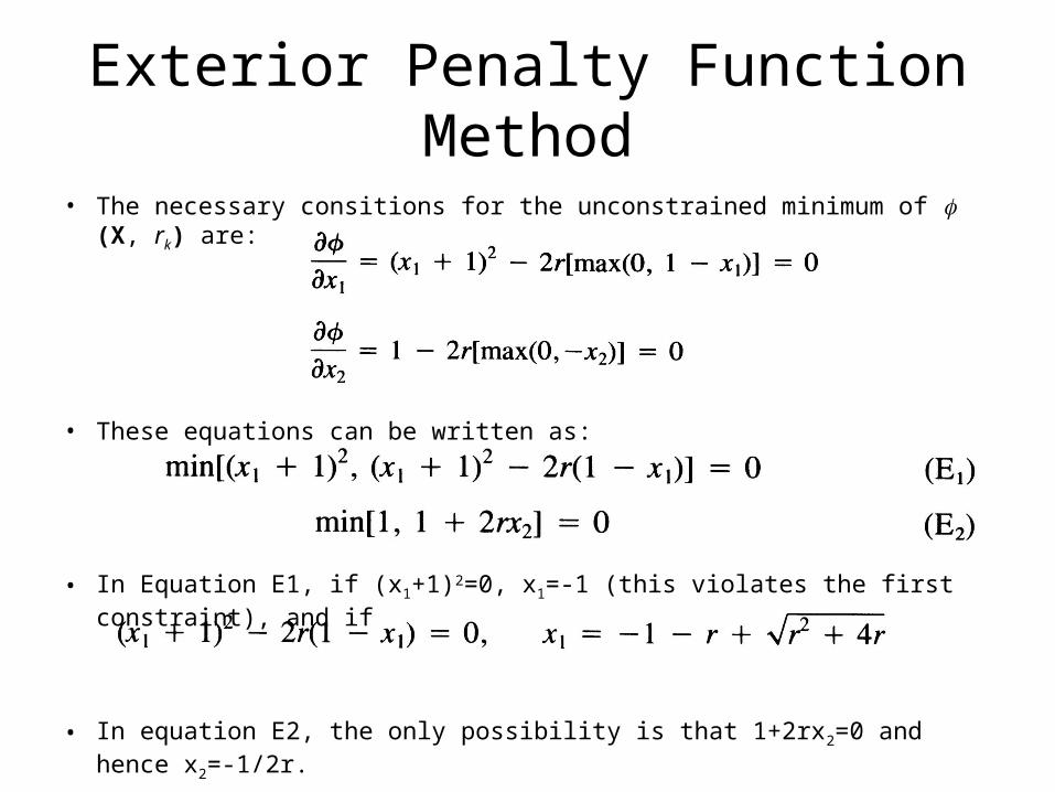
• The necessary consitions for the unconstrained minimum of (X, rk) are:
• These equations can be written as:
• In Equation E1, if (x1+1)2=0, x1=-1 (this violates the first constraint), and if
• In equation E2, the only possibility is that 1+2rx2=0 and hence x2=-1/2r.
Exterior Penalty Function Method
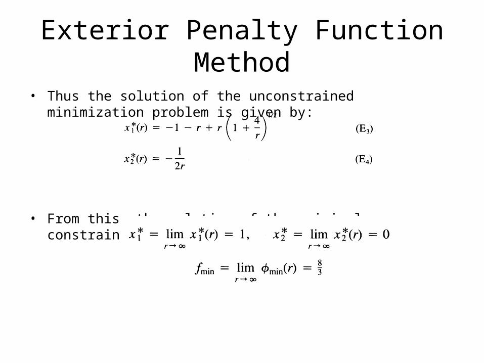
• Thus the solution of the unconstrained minimization problem is given by:
• From this, the solution of the original constrained problem can be obtained as
Exterior Penalty Function Method
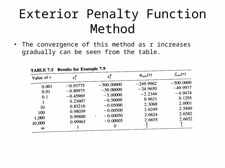
• The convergence of this method as r increases gradually can be seen from the table.
Exterior Penalty Function Method
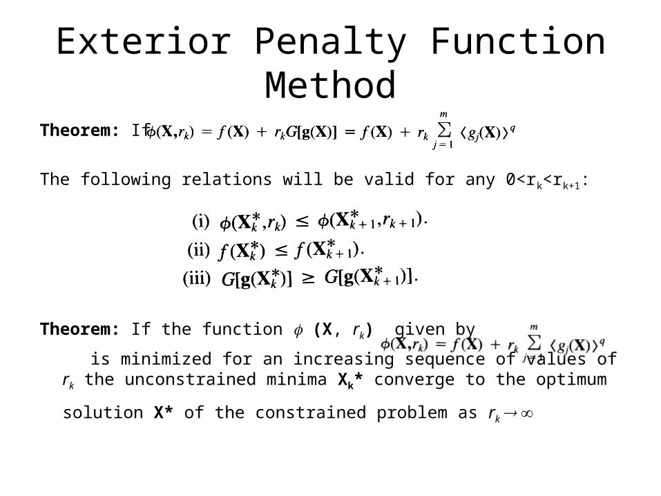
Theorem: If
The following relations will be valid for any 0<rk<rk+1:
Theorem: If the function (X, rk) given by
is minimized for an increasing sequence of values of rk the unconstrained minima Xk* converge to the optimum solution X* of the constrained
problem as rk
Extrapolation Technique in the Interior Penalty Function Method
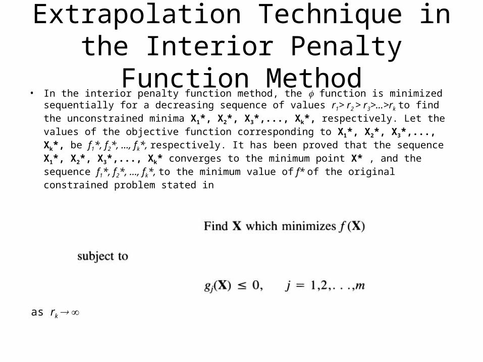
• In the interior penalty function method, the function is minimized sequentially for a decreasing sequence of values r1> r2 > r3>...>rk to find the unconstrained minima X1*, X2*, X3*,..., Xk*, respectively. Let the values of the objective function corresponding to X1*, X2*, X3*,..., Xk*, be f1*, f2*, ..., fk*, respectively. It has been proved that the sequence X1*, X2*, X3*,..., Xk* converges to the minimum point X* , and the sequence f1*, f2*, ..., fk*, to the minimum value of f* of the original constrained problem stated in
as rk
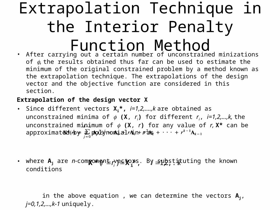
• After carrying out a certain number of unconstrained minizations of , the results obtained thus far can be used to estimate the minimum of the original constrained problem by a method known as the extrapolation technique. The extrapolations of the design vector and the objective function are considered in this section.
Extrapolation of the design vector X
• Since different vectors Xi*, i=1,2,….,k are obtained as unconstrained minima of (X, ri) for different ri, i=1,2,…,k, the unconstrained minimum of (X, r) for any value of r, X* can be approximated by a polynomial in r as
• where Aj are n-component vectors. By substituting the known conditions
in the above equation , we can determine the vectors Aj, j=0,1,2,…,k-1 uniquely.
Extrapolation Technique in the Interior Penalty Function Method
kirr i ,...,2,1*,)( iX*X
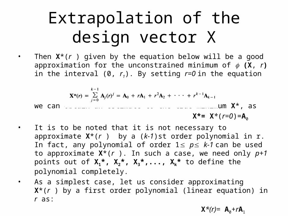
• Then X*(r ) given by the equation below will be a good approximation for the unconstrained minimum of (X, r) in the interval (0, r1). By setting r=0 in the equation
we can obtain an estimate to the true minimum X*, as
X*= X*(r=0)=A0
• It is to be noted that it is not necessary to approximate X*(r ) by a (k-1)st order polynomial in r. In fact, any polynomial of order 1 p k-1 can be used to approximate X*(r ). In such a case, we need only p+1 points out of X1*, X2*, X3*,..., Xk* to define the polynomial completely.
• As a simplest case, let us consider approximating X*(r ) by a first order polynomial (linear equation) in r as:
X*(r)= A0+rA1
Extrapolation of the design vector X
Extrapolation of the design vector X
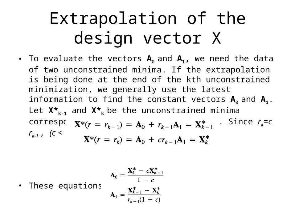
• To evaluate the vectors A0 and A1, we need the data of two unconstrained minima. If the extrapolation is being done at the end of the kth unconstrained minimization, we generally use the latest information to find the constant vectors A0 and A1. Let X*k-1 and X*k be the unconstrained minima corresponding to rk-1 and rk , respectively. Since rk=c rk-1 , (c < 1), the equation X*= A0+rA1 gives
• These equations give
Extrapolation of the design vector X
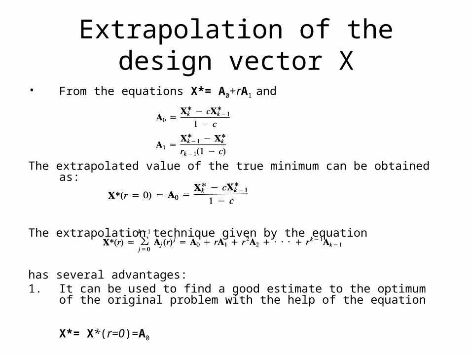
• From the equations X*= A0+rA1 and
The extrapolated value of the true minimum can be obtained as:
The extrapolation technique given by the equation
has several advantages:1. It can be used to find a good estimate to the optimum of the original problem
with the help of the equation
X*= X*(r=0)=A0
Extrapolation of the design vector X
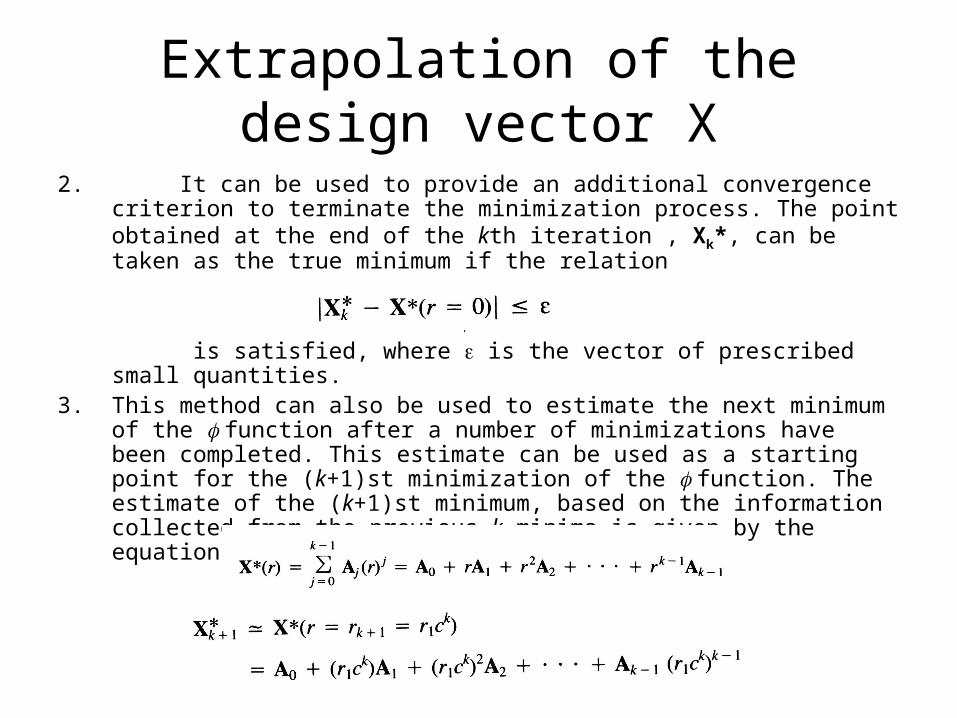
2. It can be used to provide an additional convergence criterion to terminate the minimization process. The point obtained at the end of the kth iteration , Xk*, can be taken as the true minimum if the relation
is satisfied, where is the vector of prescribed small quantities.3. This method can also be used to estimate the next minimum of the
function after a number of minimizations have been completed. This estimate can be used as a starting point for the (k+1)st minimization of the function. The estimate of the (k+1)st minimum, based on the information collected from the previous k minima is given by the equation
as
Extrapolation of the design vector X
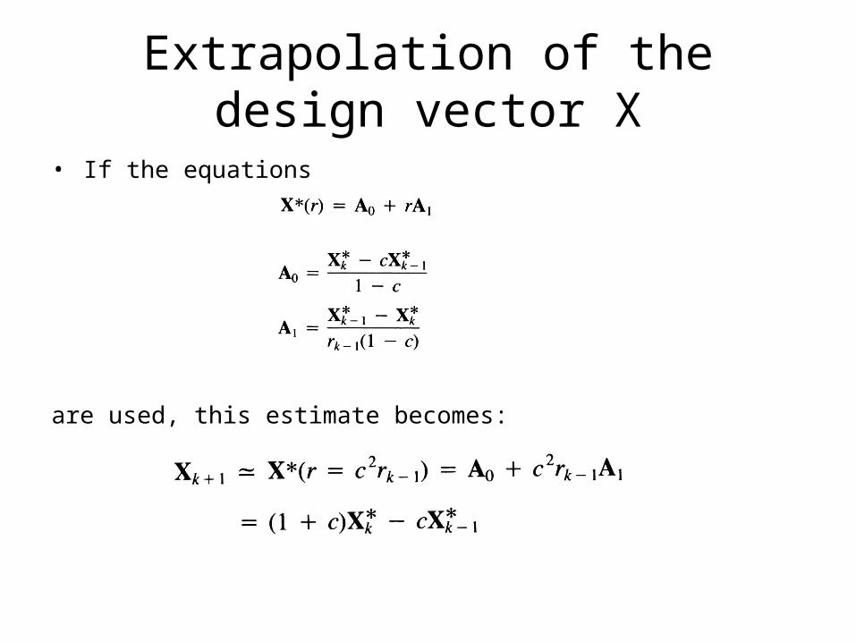
• If the equations
are used, this estimate becomes:
Extrapolation of the design vector X
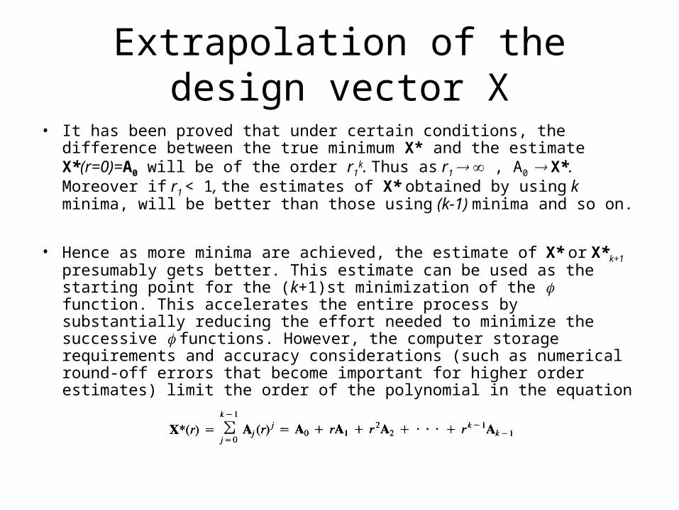
• It has been proved that under certain conditions, the difference between the true minimum X* and the estimate X*(r=0)=A0 will be of the order r1
k. Thus as r1 , A0 X*. Moreover if r1 < 1, the estimates of X* obtained by using k minima, will be better than those using (k-1) minima and so on.
• Hence as more minima are achieved, the estimate of X* or X*k+1 presumably gets better. This estimate can be used as the starting point for the (k+1)st minimization of the function. This accelerates the entire process by substantially reducing the effort needed to minimize the successive functions. However, the computer storage requirements and accuracy considerations (such as numerical round-off errors that become important for higher order estimates) limit the order of the polynomial in the equation
Extrapolation of the design vector X
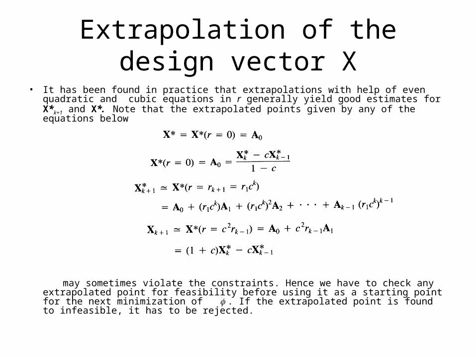
• It has been found in practice that extrapolations with help of even quadratic and cubic equations in r generally yield good estimates for X*k+1 and X*. Note that the extrapolated points given by any of the equations below
may sometimes violate the constraints. Hence we have to check any extrapolated point for feasibility before using it as a starting point for the next minimization of . If the extrapolated point is found to infeasible, it has to be rejected.
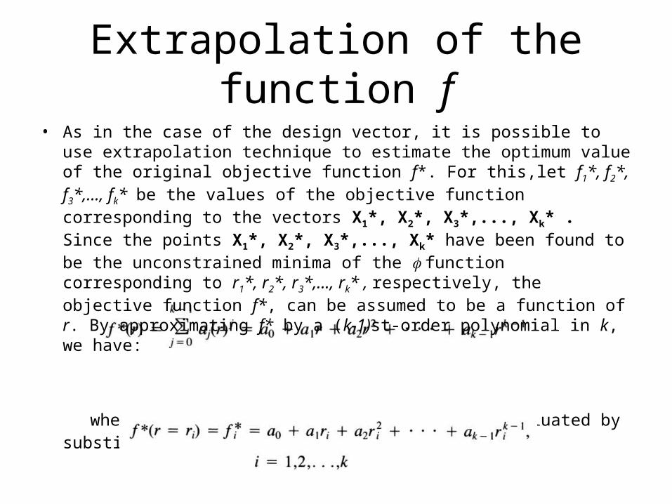
• As in the case of the design vector, it is possible to use extrapolation technique to estimate the optimum value of the original objective function f*. For this,let f1*, f2*, f3*,..., fk* be the values of the objective function corresponding to the vectors X1*, X2*, X3*,..., Xk* . Since the points X1*, X2*, X3*,..., Xk* have been found to be the unconstrained minima of the function corresponding to r1*, r2*, r3*,..., rk* , respectively, the objective function f*, can be assumed to be a function of r. By approximating f* by a (k-1)st-order polynomial in k, we have:
where the k constants aj, j=0,1,2,…,k-1 can be evaluated by substituting the known conditions
Extrapolation of the function f
Extrapolation of the function f
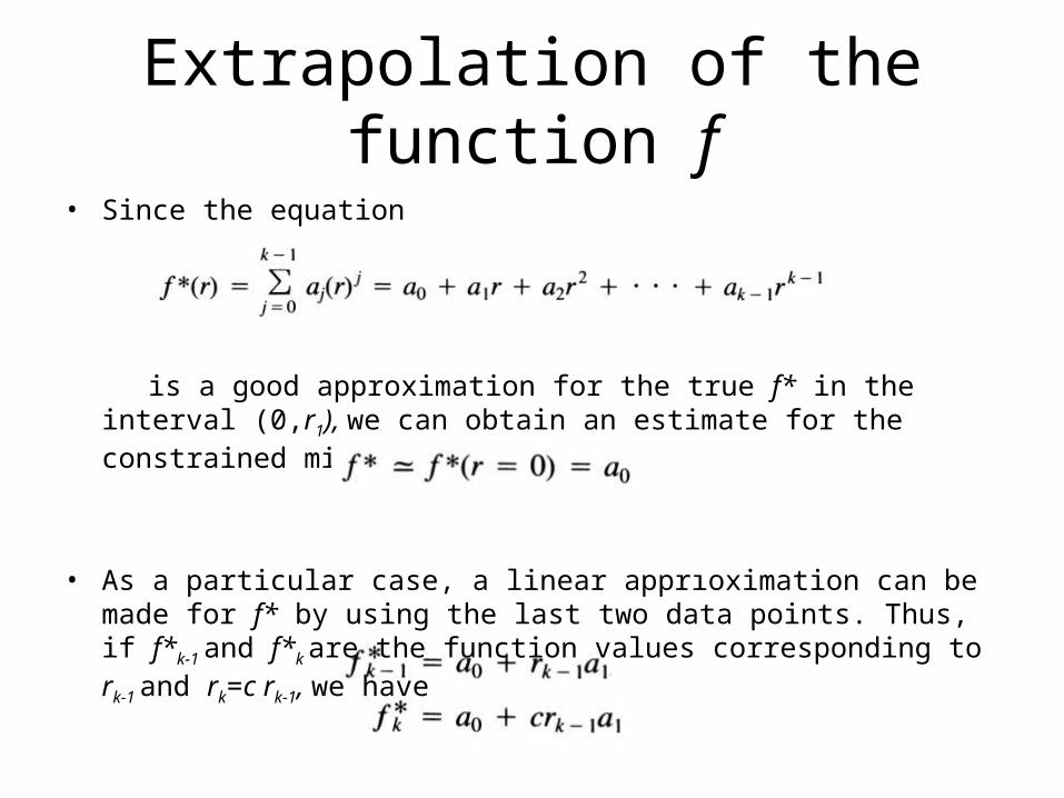
• Since the equation
is a good approximation for the true f* in the interval (0,r1), we can obtain an estimate for the constrained minimum of f as:
• As a particular case, a linear apprıoximation can be made for f* by using the last two data points. Thus, if f*k-1 and f*k are the function values corresponding to rk-1 and rk=c rk-1, we have
Extrapolation of the function f
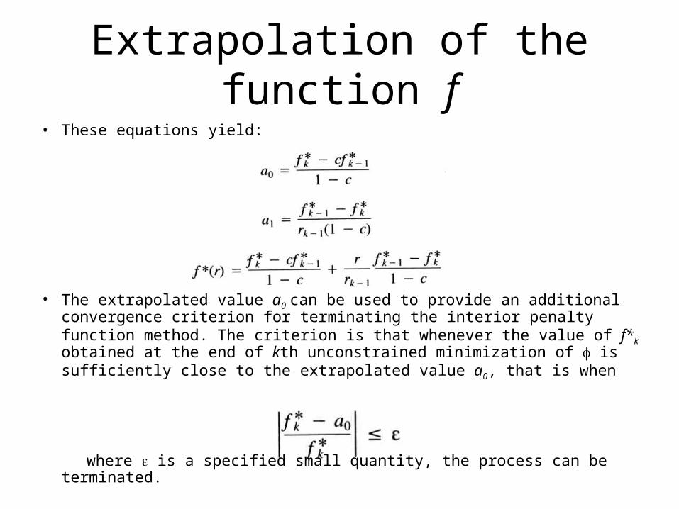
• These equations yield:
• The extrapolated value a0 can be used to provide an additional convergence criterion for terminating the interior penalty function method. The criterion is that whenever the value of f*k obtained at the end of kth unconstrained minimization of is sufficiently close to the extrapolated value a0, that is when
where is a specified small quantity, the process can be terminated.
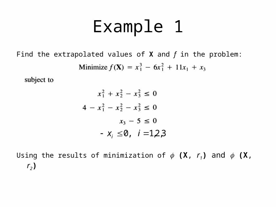
Example 1
Find the extrapolated values of X and f in the problem:
Using the results of minimization of (X, r1) and (X, r2)
3,2,1,0 ixi
Example 1
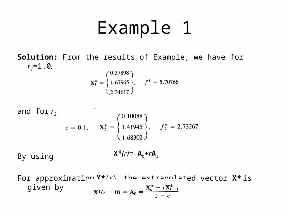
Solution: From the results of Example, we have for r1=1.0,
and for r2 = 1, we have
By using
For approximating X*(r), the extrapolated vector X* is given by
X*(r)= A0+rA1
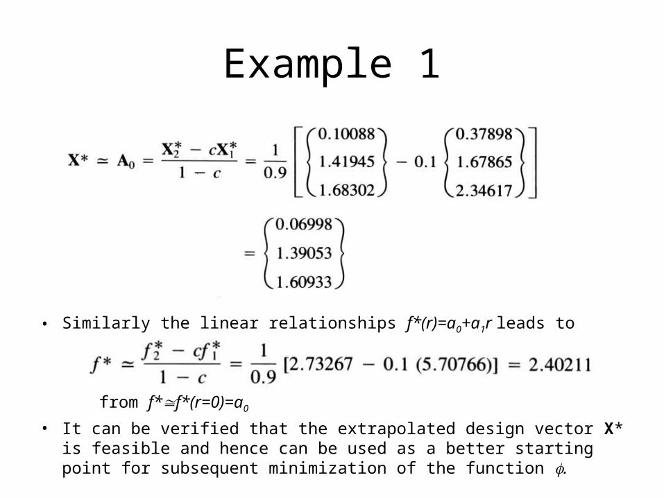
Example 1
• Similarly the linear relationships f*(r)=a0+a1r leads to
from f*f*(r=0)=a0
• It can be verified that the extrapolated design vector X* is feasible and hence can be used as a better starting point for subsequent minimization of the function .
Extended interior penalty function methods
• In the interior penalty function approach, the function is defined within the feasible domain. As such, if any of the one-dimensional minimization methods discussed before is used, the resulting optimal step lengths might lead to infeasible designs. Thus, the one-dimensional minimization methods have to be modified to avoid this problem.
• An alternative method known as the extended interior penalty function method, has been proposed in which the function is defined outside the feasible region.
• The extended interior penalty function method combines the best features of the interior and exterior methods for inequality constraints. Several types of extended interior penalty function formulations are described in this section.
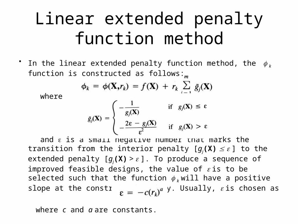
• In the linear extended penalty function method, the k function is constructed as follows:
where
and is a small negative number that marks the transition from the interior penalty [gj(X) ] to the extended penalty [gj(X) > ]. To produce a sequence of improved feasible designs, the value of is to be selected such that the function k will have a positive slope at the constraint boundary. Usually, is chosen as
where c and a are constants.
Linear extended penalty function method
Linear extended penalty function method
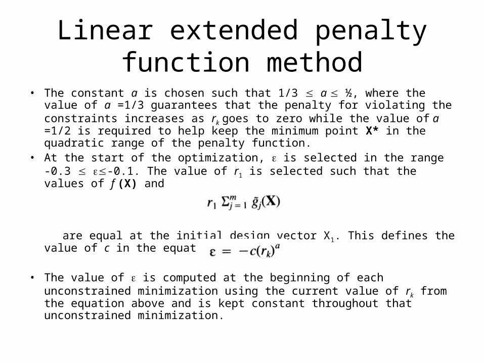
• The constant a is chosen such that 1/3 a ½, where the value of a =1/3 guarantees that the penalty for violating the constraints increases as rk goes to zero while the value of a =1/2 is required to help keep the minimum point X* in the quadratic range of the penalty function.
• At the start of the optimization, is selected in the range -0.3 -0.1. The value of r1 is selected such that the values of f (X) and
are equal at the initial design vector X1. This defines the value of c in the equation
• The value of is computed at the beginning of each unconstrained minimization using the current value of rk from the equation above and is kept constant throughout that unconstrained minimization.
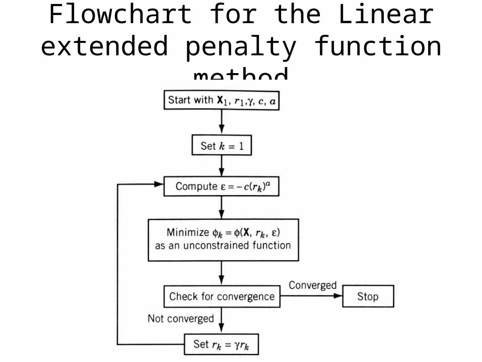
Flowchart for the Linear extended penalty function method
• The k function defined by the equation
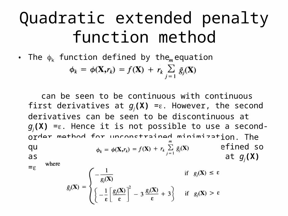
can be seen to be continuous with continuous first derivatives at gj(X) =. However, the second derivatives can be seen to be discontinuous at gj(X) =. Hence it is not possible to use a second-order method for unconstrained minimization. The quadratic extended penalty function is defined so as to have continuous second derivatives at gj(X) = as follows:
Quadratic extended penalty function method
Quadratic extended penalty function method
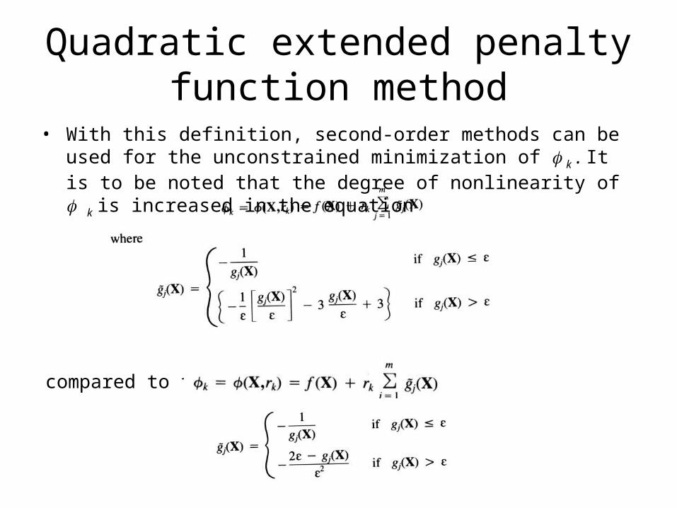
• With this definition, second-order methods can be used for the unconstrained minimization of k . It is to be noted that the degree of nonlinearity of k is increased in the equation
compared to the equation
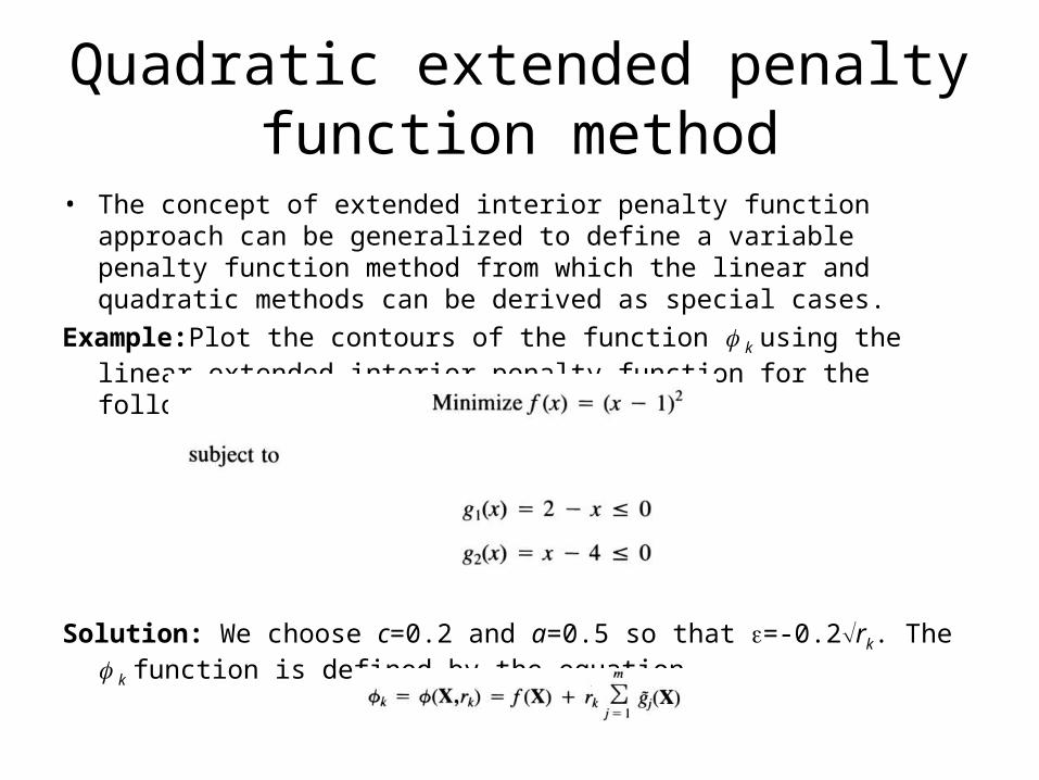
• The concept of extended interior penalty function approach can be generalized to define a variable penalty function method from which the linear and quadratic methods can be derived as special cases.
Example:Plot the contours of the function k using the linear extended interior penalty function for the following problem:
Solution: We choose c=0.2 and a=0.5 so that =-0.2rk. The k function is defined by the equation
Quadratic extended penalty function method
Quadratic extended penalty function method
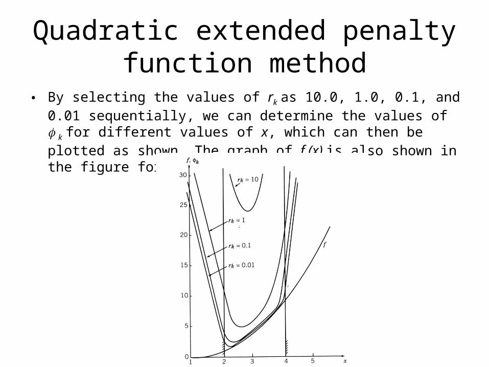
• By selecting the values of rk as 10.0, 1.0, 0.1, and 0.01 sequentially, we can determine the values of k for different values of x, which can then be plotted as shown. The graph of f (x) is also shown in the figure for comparison:
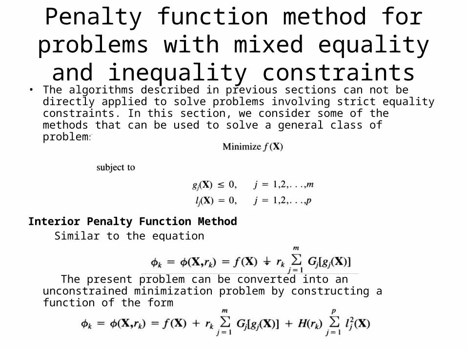
• The algorithms described in previous sections can not be directly applied to solve problems involving strict equality constraints. In this section, we consider some of the methods that can be used to solve a general class of problems.
Interior Penalty Function Method Similar to the equation
The present problem can be converted into an unconstrained minimization problem by constructing a function of the form
Penalty function method for problems with mixed equality and inequality constraints
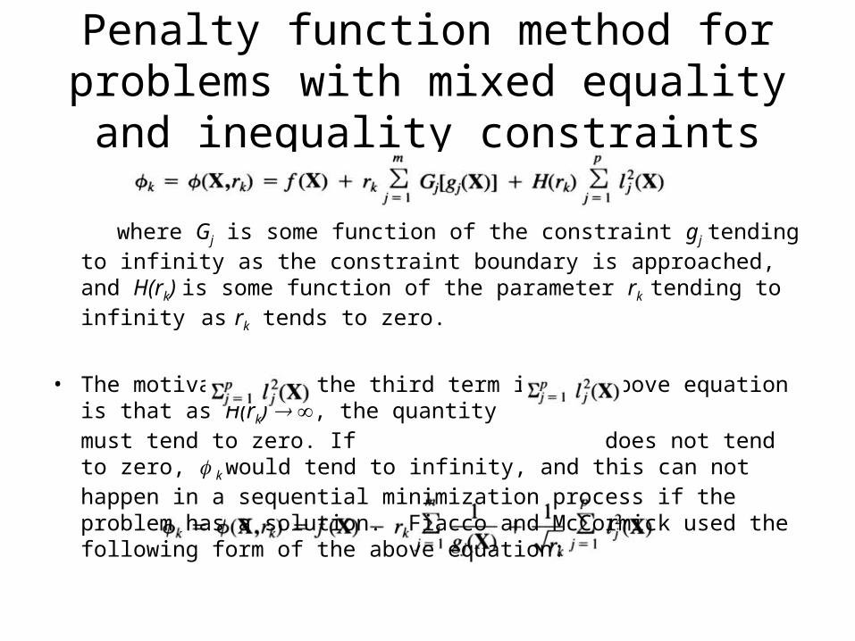
where Gj is some function of the constraint gj tending to infinity as the constraint boundary is approached, and H(rk) is some function of the parameter rk tending to infinity as rk tends to zero.
• The motivation of the third term in the above equation is that as H(rk) , the quantity must tend to zero. If does not tend to zero, k would tend to infinity, and this can not happen in a sequential minimization process if the problem has a solution. Fiacco and McCormick used the following form of the above equation:
Penalty function method for problems with mixed equality and inequality constraints
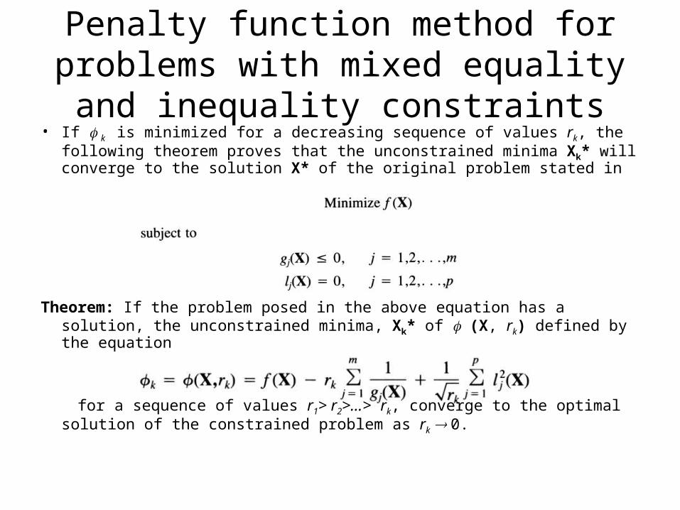
• If k is minimized for a decreasing sequence of values rk, the following theorem proves that the unconstrained minima Xk* will converge to the solution X* of the original problem stated in
Theorem: If the problem posed in the above equation has a solution, the unconstrained minima, Xk* of (X, rk) defined by the equation
for a sequence of values r1> r2>...> rk, converge to the optimal solution of the constrained problem as rk 0.
Penalty function method for problems with mixed equality and inequality constraints
Penalty function method for problems with mixed equality and inequality constraints
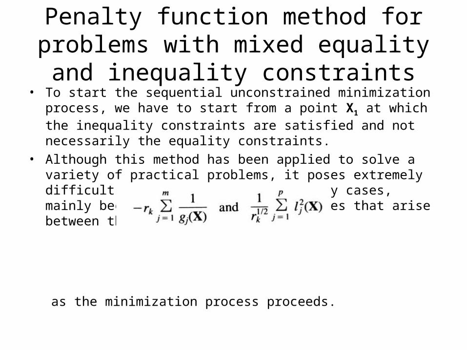
• To start the sequential unconstrained minimization process, we have to start from a point X1 at which the inequality constraints are satisfied and not necessarily the equality constraints.
• Although this method has been applied to solve a variety of practical problems, it poses extremely difficult minimization problem in many cases, mainly because of the scale disparities that arise between the penalty terms
as the minimization process proceeds.
Exterior Penalty Function Method
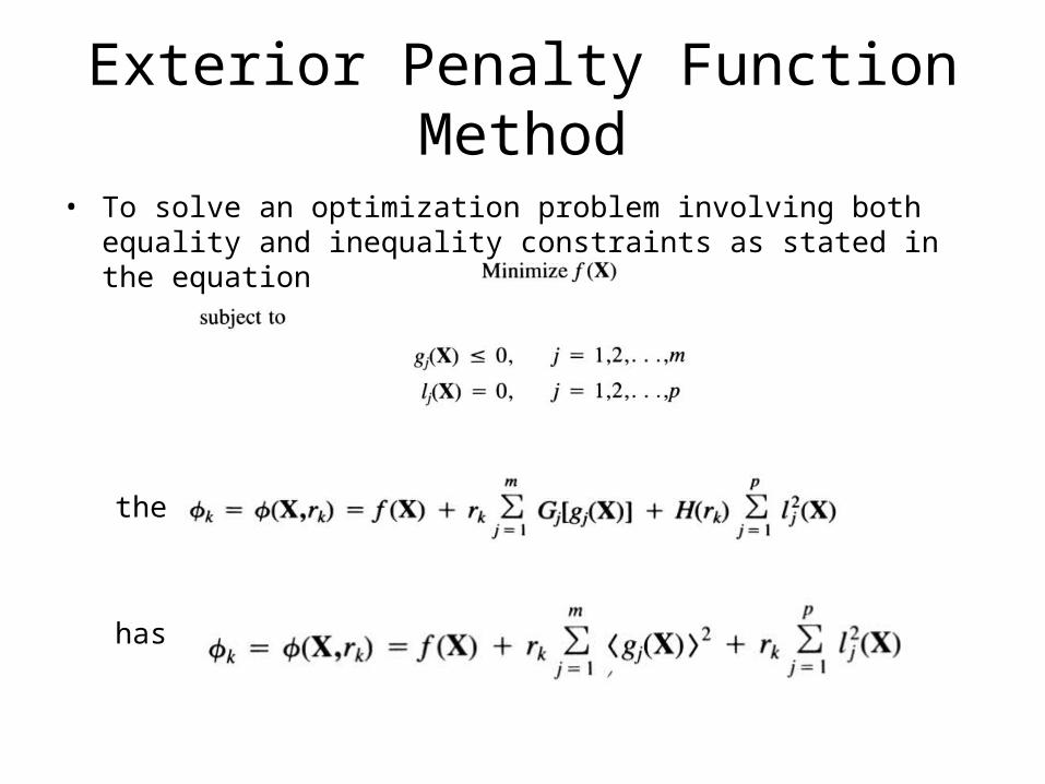
• To solve an optimization problem involving both equality and inequality constraints as stated in the equation
the following form of the equation
has been proposed:
Exterior Penalty Function Method
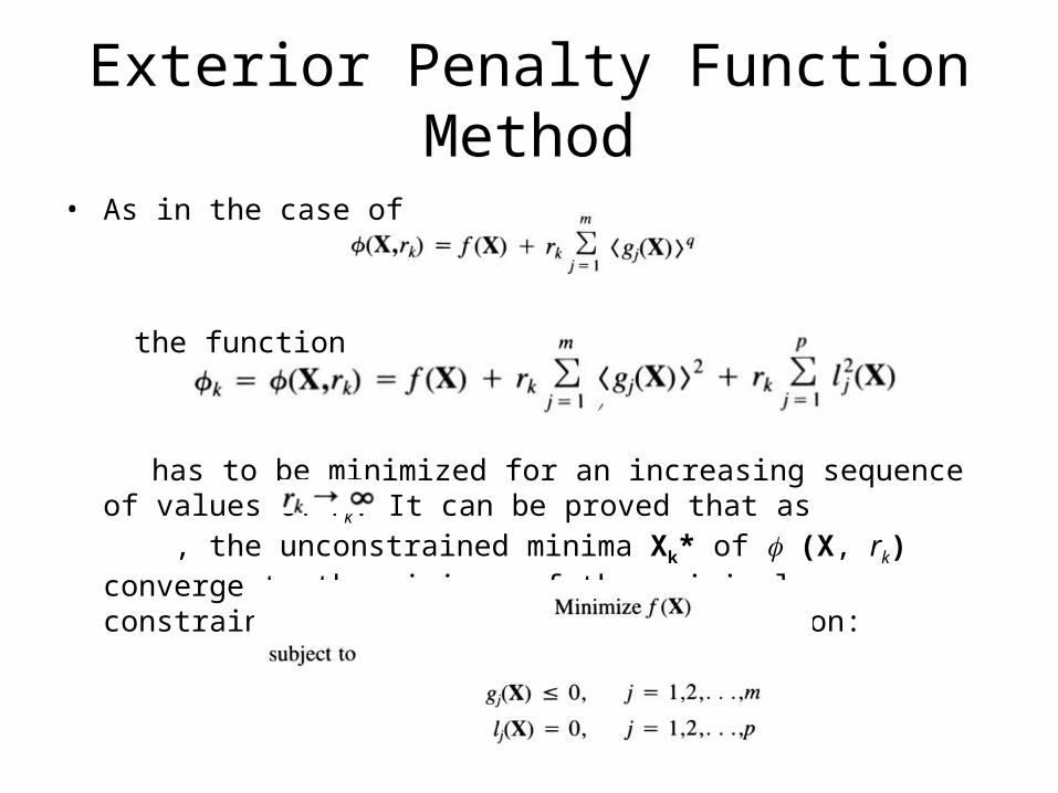
• As in the case of
the function
has to be minimized for an increasing sequence of values of rk. It can be proved that as , the unconstrained minima Xk* of (X, rk) converge to the minimum of the original constrained problem stated in the equation:
Penalty function method for parametric constraints
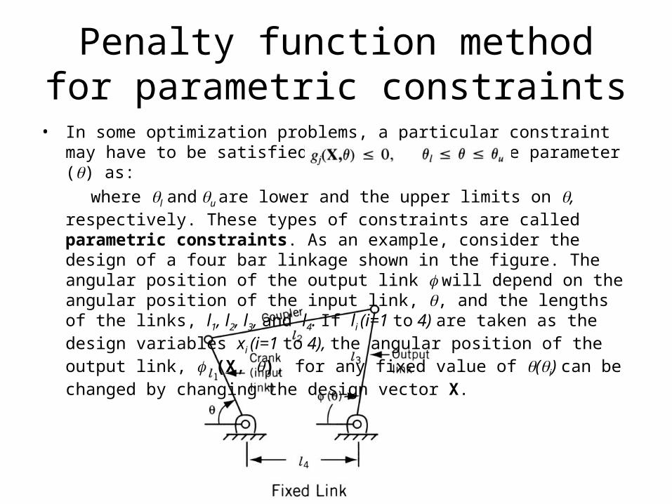
• In some optimization problems, a particular constraint may have to be satisfied over a range of some parameter () as:
where l and u are lower and the upper limits on , respectively. These types of constraints are called parametric constraints. As an example, consider the design of a four bar linkage shown in the figure. The angular position of the output link will depend on the angular position of the input link, , and the lengths of the links, l1, l2, l3, and l4. If li (i=1 to 4) are taken as the design variables xi (i=1 to 4), the angular position of the output link, (X, ), for any fixed value of (i) can be changed by changing the design vector X.
Penalty function method for parametric constraints
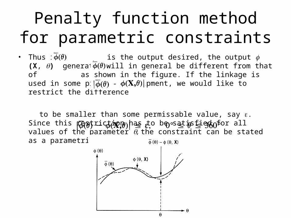
• Thus if is the output desired, the output (X, ) generated will in general be different from that of as shown in the figure. If the linkage is used in some precision equipment, we would like to restrict the difference
to be smaller than some permissable value, say . Since this restriction has to be satisfied for all values of the parameter , the constraint can be stated as a parametric constraint
Penalty function method for parametric constraints
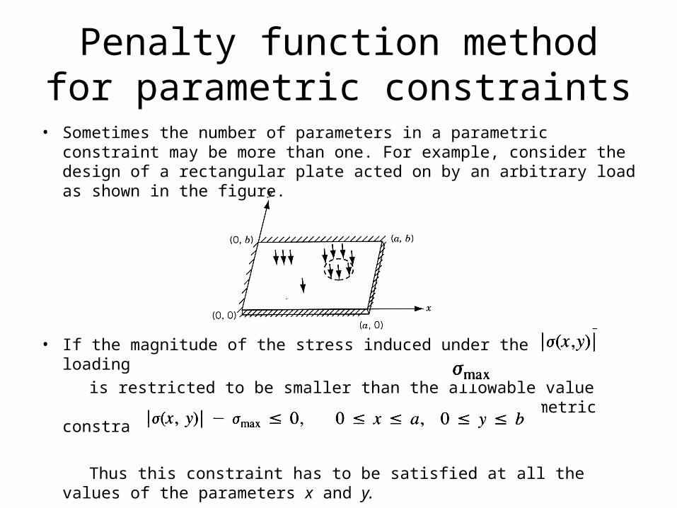
• Sometimes the number of parameters in a parametric constraint may be more than one. For example, consider the design of a rectangular plate acted on by an arbitrary load as shown in the figure.
• If the magnitude of the stress induced under the given loading
is restricted to be smaller than the allowable value , the constraint can be stated as a parametric constraint as
Thus this constraint has to be satisfied at all the values of the parameters x and y.
Penalty function method for parametric constraints
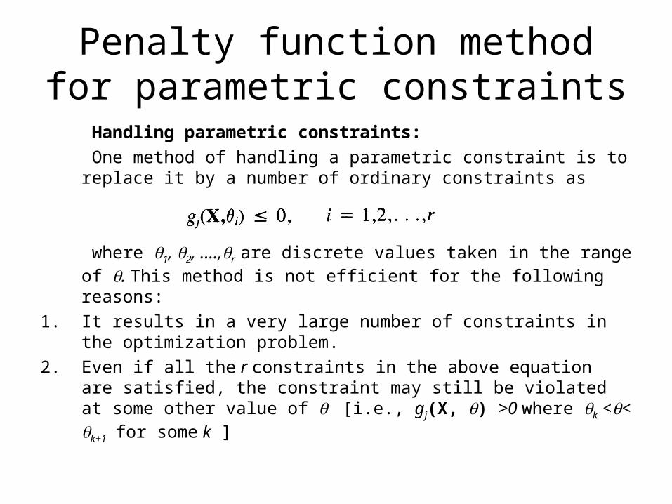
Handling parametric constraints:
One method of handling a parametric constraint is to replace it by a number of ordinary constraints as
where 1, 2, ….,r are discrete values taken in the range of . This method is not efficient for the following reasons:
1. It results in a very large number of constraints in the optimization problem.
2. Even if all the r constraints in the above equation are satisfied, the constraint may still be violated at some other value of [i.e., gj(X, ) >0 where k << k+1 for some k ]
Penalty function method for parametric constraints
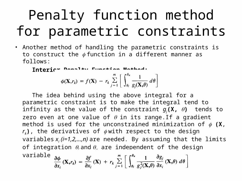
• Another method of handling the parametric constraints is to construct the function in a different manner as follows:
Interior Penalty Function Method:
The idea behind using the above integral for a parametric constraint is to make the integral tend to infinity as the value of the constraint gj(X, ) tends to zero even at one value of in its range.If a gradient method is used for the unconstrained minimization of (X, rk), the derivatives of with respect to the design variables xi (i=1,2,…,n) are needed. By assuming that the limits of integration l and u are independent of the design variables xi, the above equation gives:
Penalty function method for parametric constraints
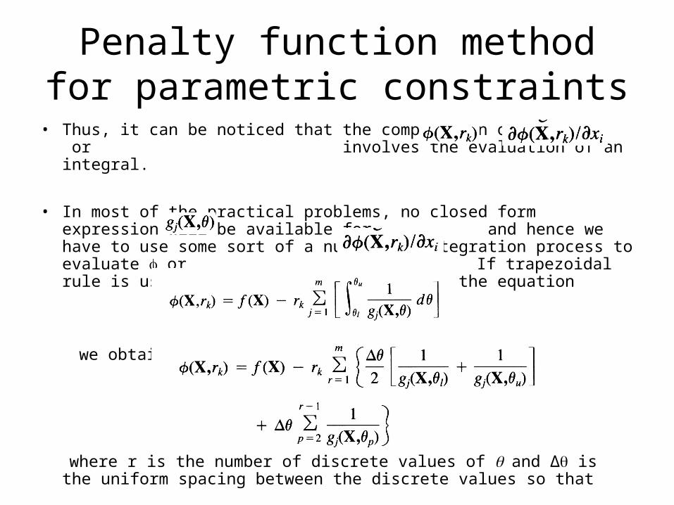
• Thus, it can be noticed that the computation of or involves the evaluation of an integral.
• In most of the practical problems, no closed form expression will be available for and hence we have to use some sort of a numerical integration process to evaluate or If trapezoidal rule is used to evaluate the integral in the equation
we obtain:
where r is the number of discrete values of and Δ is the uniform spacing between the discrete values so that
Penalty function method for parametric constraints
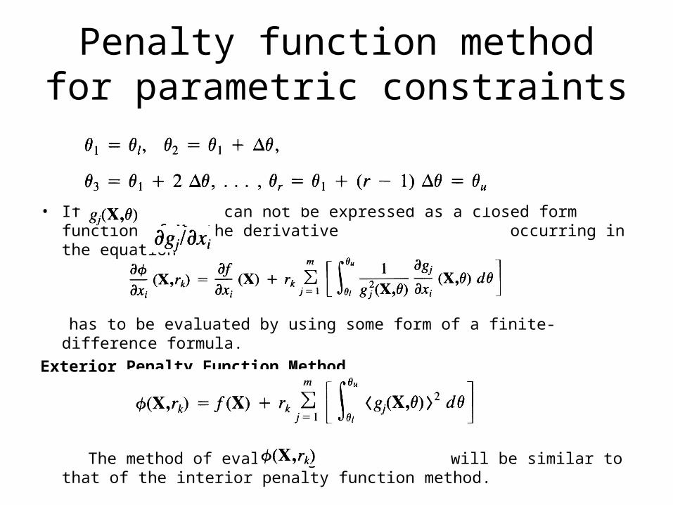
• If can not be expressed as a closed form function of X, the derivative occurring in the equation
has to be evaluated by using some form of a finite-difference formula.
Exterior Penalty Function Method
The method of evaluating will be similar to that of the interior penalty function method.
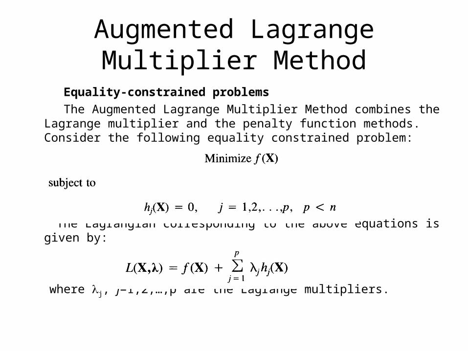
Equality-constrained problems
The Augmented Lagrange Multiplier Method combines the Lagrange multiplier and the penalty function methods. Consider the following equality constrained problem:
The Lagrangian corresponding to the above equations is given by:
where j, j=1,2,…,p are the Lagrange multipliers.
Augmented Lagrange Multiplier Method
Augmented Lagrange Multiplier Method
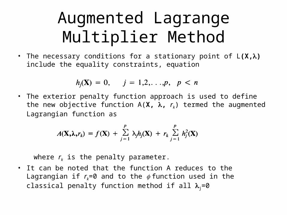
• The necessary conditions for a stationary point of L(X,) include the equality constraints, equation
• The exterior penalty function approach is used to define the new objective function A(X, , rk) termed the augmented Lagrangian function as
where rk is the penalty parameter.
• It can be noted that the function A reduces to the Lagrangian if rk=0 and to the function used in the classical penalty function method if all j=0
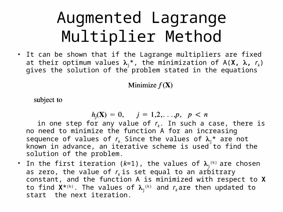
Augmented Lagrange Multiplier Method
• It can be shown that if the Lagrange multipliers are fixed at their optimum values j*, the minimization of A(X, , rk) gives the solution of the problem stated in the equations
in one step for any value of rk. In such a case, there is no need to minimize the function A for an increasing sequence of values of rk. Since the values of j* are not known in advance, an iterative scheme is used to find the solution of the problem.
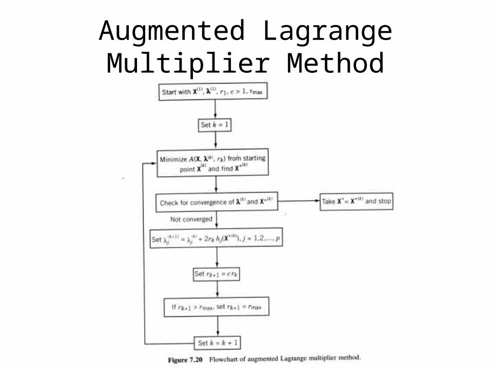
• In the first iteration (k=1), the values of j(k) are chosen as zero, the value of
rk is set equal to an arbitrary constant, and the function A is minimized with respect to X to find X*(k). The values of j
(k) and rk are then updated to start the next iteration.
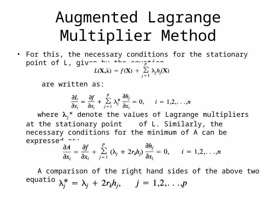
Augmented Lagrange Multiplier Method
• For this, the necessary conditions for the stationary point of L, given by the equation
are written as:
where j* denote the values of Lagrange multipliers at the stationary point of L. Similarly, the necessary conditions for the minimum of A can be expressed as:
A comparison of the right hand sides of the above two equations yield:
Augmented Lagrange Multiplier Method
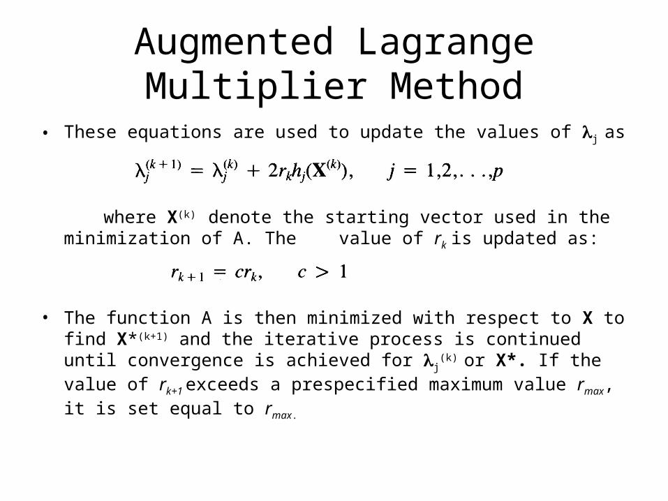
• These equations are used to update the values of j as
where X(k) denote the starting vector used in the minimization of A. The value of rk is updated as:
• The function A is then minimized with respect to X to find X*(k+1) and the iterative process is continued until convergence is achieved for j
(k) or X*. If the value of rk+1 exceeds a prespecified maximum value rmax, it is set equal to rmax.
Augmented Lagrange Multiplier Method
Augmented Lagrange Multiplier Method
Inequality constrained problems
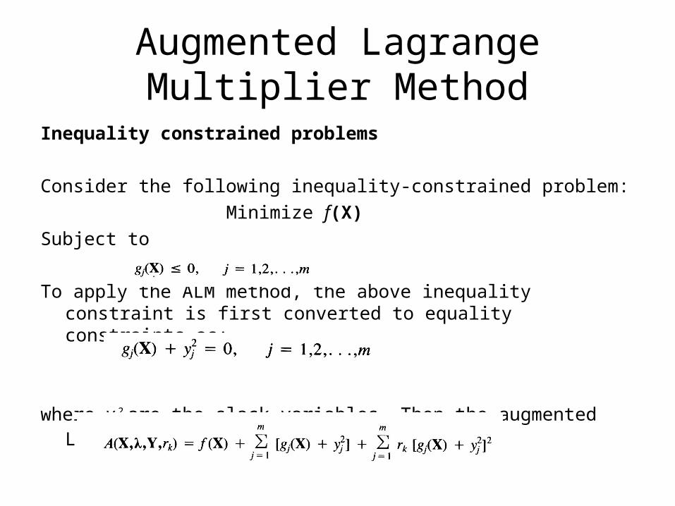
Consider the following inequality-constrained problem:
Minimize f(X)
Subject to
To apply the ALM method, the above inequality constraint is first converted to equality constraints as:
where yj2 are the slack variables. Then the augmented Lagrangian function is
constructed as:
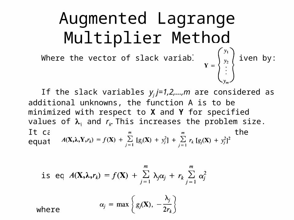
Where the vector of slack variables Y is given by:
If the slack variables yj j=1,2,…,m are considered as additional unknowns, the function A is to be minimized with respect to X and Y for specified values of j and rk. This increases the problem size. It can be shown that the function A given by the equation
is equivalent to
where
Augmented Lagrange Multiplier Method
Augmented Lagrange Multiplier Method
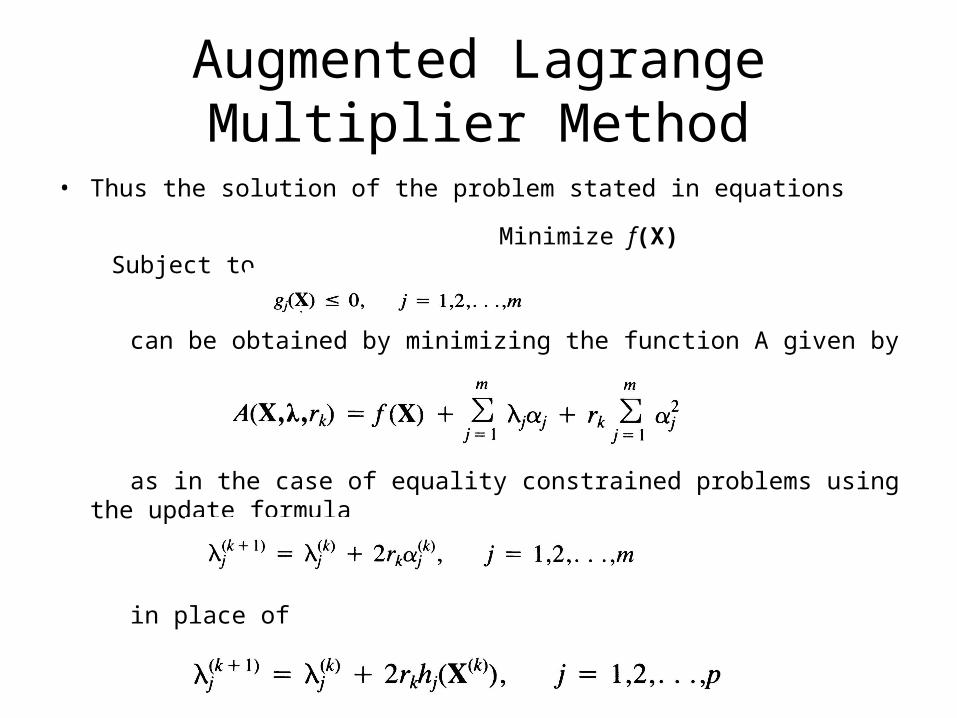
• Thus the solution of the problem stated in equations
can be obtained by minimizing the function A given by
as in the case of equality constrained problems using the update formula
in place of
Minimize f(X)Subject to
Augmented Lagrange Multiplier Method
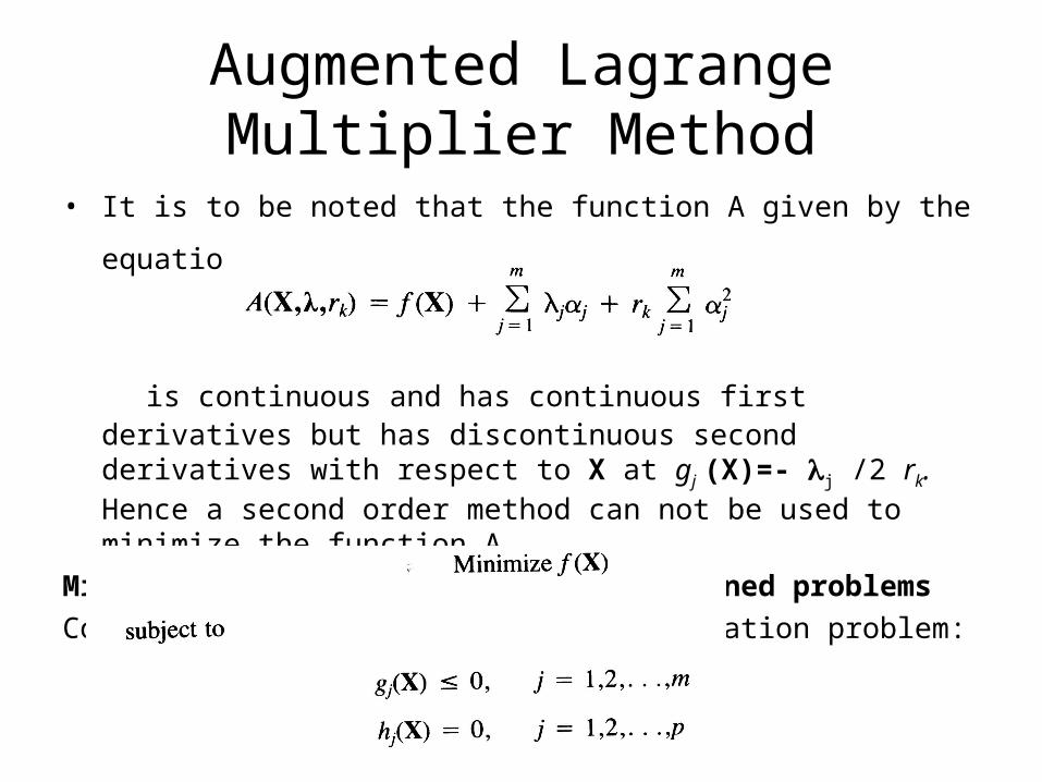
• It is to be noted that the function A given by the equation
is continuous and has continuous first derivatives but has discontinuous second derivatives with respect to X at gj (X)=- j /2 rk. Hence a second order method can not be used to minimize the function A.
Mixed equality and inequality constrained problems
Consider the following general optimization problem:
• This problem can be solved by combining the procedures of the two preceding sections. The augmented Lagrangian function is defined as:
where is given by:
• The solution of the given problem above can be found by minimizing the function A as in the case of equality constrained problems using the update formula:
Augmented Lagrange Multiplier Method
Augmented Lagrange Multiplier Method
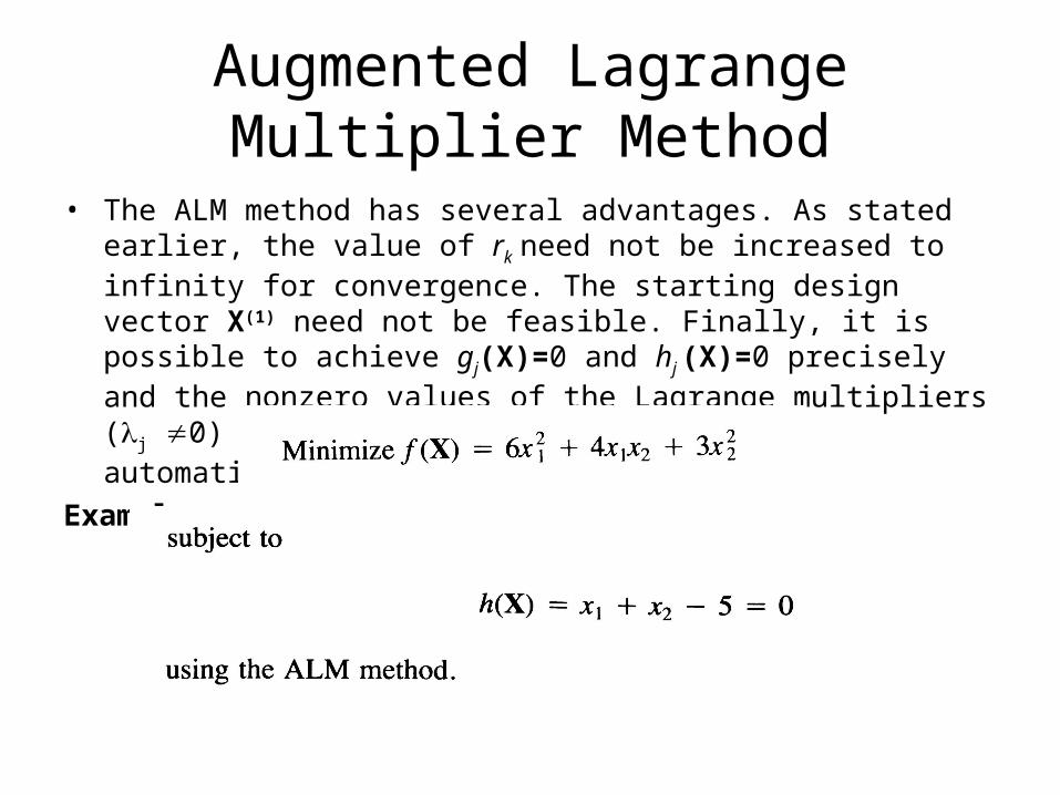
• The ALM method has several advantages. As stated earlier, the value of rk need not be increased to infinity for convergence. The starting design vector X(1) need not be feasible. Finally, it is possible to achieve gj(X)=0 and hj (X)=0 precisely and the nonzero values of the Lagrange multipliers (j 0) identify the active constraints automatically.
Example:
Augmented Lagrange Multiplier Method
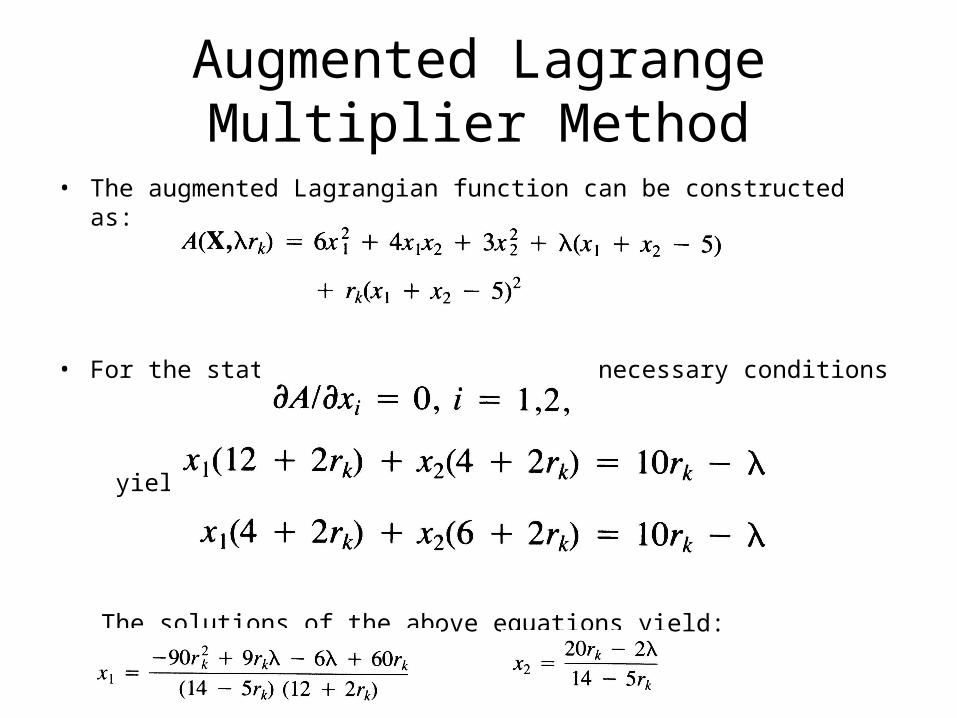
• The augmented Lagrangian function can be constructed as:
• For the stationary point of A, the necessary conditions
yield
The solutions of the above equations yield:
Augmented Lagrange Multiplier Method
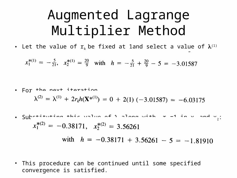
• Let the value of rk be fixed at 1and select a value of (1) =0. This gives
• For the next iteration
• Substituting this value of along with rk =1 in x1 and x2:
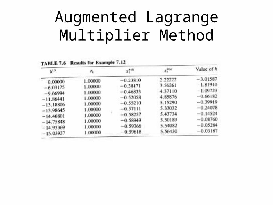
• This procedure can be continued until some specified convergence is satisfied.
Augmented Lagrange Multiplier Method


![Nonlinear Programming Models Fabio Schoen Introductionfor all x,y ∈ Ω,λ ∈ [0,1] Nonlinear Programming Models – p. 5 Convex Functions x y Nonlinear Programming Models – p](https://img.pdfslide.us/doc/110x75/60025c042470c9743d105bb3/nonlinear-programming-models-fabio-schoen-for-all-xy-a-a-01-nonlinear.jpg)