1

Nonlinear phenomena in optical fibers

Halina Abramczyk

Technical University of Lodz, Laboratory of Laser Molecular Spectroscopy, 93- 590 Lodz,

Wroblewskiego 15 str, Poland, abramczy@mitr.p.lodz.pl, www.mitr.p.lodz.pl/raman

, www.mitr.p.lodz.pl/evu

Max Born Institute, Marie Curie Chair, 12489 Berlin, Max Born Str 2A, abramczy@mbi-

berlin.de

4. Nonlinear phenomena

4.1. Second-order nonlinear phenomena

4.2. Third-order nonlinear phenomena

4.3. Stimulated Raman scattering

4.4. Stimulated Brillouin scattering

4.5. Four-wave mixing (FWM)

4.6. Self-phase modulation (SPM)

4.7. Cross phase modulation (XPM)

4.8. Theoretical description of GVD phenomenon and self-phase modulation

4.8.1. Nonlinear Schrödinger equation

4.8.2. Inclusion of the higher order nonlinear effects in the nonlinear Schrödinger

equation

4.8.3. Derivation of formula for pulse broadening due to the GVD effect

4. Nonlinear phenomena

For many years the nonlinear phenomena were the matter of concern for relatively

narrow circle of professionals dealing with the laser spectroscopy. So far, Raman scattering

phenomena have widely been used in chemistry, materials engineering, and physics for

research on the nature of interactions, chemical bonds and properties of semiconductors.

During the last decade the interest in the stimulated Raman scattering and other nonlinear

optical phenomena has significantly increased with the development of optical

telecommunication. After 2000, almost all systems (long-haul – defined as 300 to 800 km

and ultralong-haul – above 800km) have been using Raman amplification, substituting the

most conventional in nineties EDFAs, erbium-doped fibre amplifiers. Despite the Raman

amplification phenomenon had been demonstrated in optical waveguides by Stolen and Ippen

in the beginning of seventies [1], the eighties and the former half of nineties were dominated

by EDFA amplifiers. In the latter half of nineties the increase of interest in Raman amplifiers

occurred. Evidently, the physics of Raman scattering phenomenon has remained the same

since Raman and Krishnan publication in Nature in 1929 [2]. However, for the phenomenon

to be applied there has to occur the significant progress in the optical waveguide technologies

[3-5].

The radiation emitted by conventional light sources like electric bulbs, photoflash

lamps, etc., is neither monochromatic nor coherent in time and space. Intensity of electric

field of radiation emitted by conventional light sources is small (10-103 V/cm). Radiation of

such intensity, when interacting with matter (reflection of light, scattering, absorption and

refraction of light), does not change its macro- and microscopic properties, because it is

several orders of magnitude smaller than the intensity of electric field in matter (of the order

2

of 109 V/cm). The intensity of laser light, in particular generated by pulse lasers emitting short

pulses, can reach values of the order of 1012

W/cm2 that corresponds to the intensity of the

electric field of radiation of 105 to 10

8 V/cm. It is therefore comparable to the intensity of

electric fields in matters.

Weak electric fields E of radiation generate electric induction D,

PED π4 , (4.1)

which depends on the polarisation of a medium P. For small values of light intensities, the

polarisation is linearly related to the intensity of electric field E:

EP1

, (4.2)

where 1

- electric susceptibility.

The above formula arises from the fact that the medium polarisation P is a sum of orientation

polarisation orient

P )3

(2

orientE

kTNP

and induced polarisation

indP

)(ind

ENP .

If the intensity of the electric field E increases, the medium polarisation is no longer

linearly dependent on E and should be expressed by the formula

...EEEP 33221

(4.3)

For the correctness of notation, the above formula can be rewritten taking into account the

fact that the electric susceptibility is not a scalar but a tensor:

...EEEEEEP lkjijklkjijkjiji 321

(4.4)

For the repeated subscripts of and the field intensity E, the summation over the x,y,z

components of the field intensity should be done. If several weak electric fields act on a

medium (e.g. a few leaser beams), the electric polarisation in a linear approximation is a sum

of polarisation components of individual fields:

...tttt ,,,, rPrPrPrP 321 (4.5)

It means that the weak electric fields meet the superposition principle, according to which the

electromagnetic waves propagate in a medium independently, without mutual interaction. All

the optical phenomena that can be approximated by that principle are called the linear optical

phenomena. In case of strong electric fields the approximation (4.5) is not valid. The electric

fields do not meet the superposition principle any longer. All the optical phenomena not

meeting the superposition principle are called the nonlinear optical phenomena. An example

of the nonlinear phenomenon is the dependence of the refractive index n on light intensity

(Kerr effect). For low intensities of light the index is constant. However, if a medium is

exposed to the light of the high intensity this is no longer valid and the refractive index is

proportional to E2

and makes liquids birefringent like crystals. Another example of linear

phenomena is the absorption Lambert-Beer law

)exp(0 clI/IT (4.6)

or

clT

A 1

ln , (4.7)

where T is the transmittance of a system and it corresponds to the ratio of the output beam

intensity I that went through the medium to the input beam I0, - absorption coefficient, c –

concentration of substance absorbing the light, l –length of an optical path. Within the linear

optics the absorption coefficient does not depend on light intensity. For higher light intensities

the absorption coefficient does depend on that intensity.

3

4.1. Second-order nonlinear phenomena [6]

The second-order nonlinear phenomena are described by the second term of the

equation (4.4):

kjijkiEEP

)2( (4.8)

The most often employed second-order nonlinear phenomena are as follows: a) second

harmonic generation, b) frequency mixing, c) parametric amplification. The detailed

discussion of the second-order nonlinear phenomena can be found elsewhere [4].

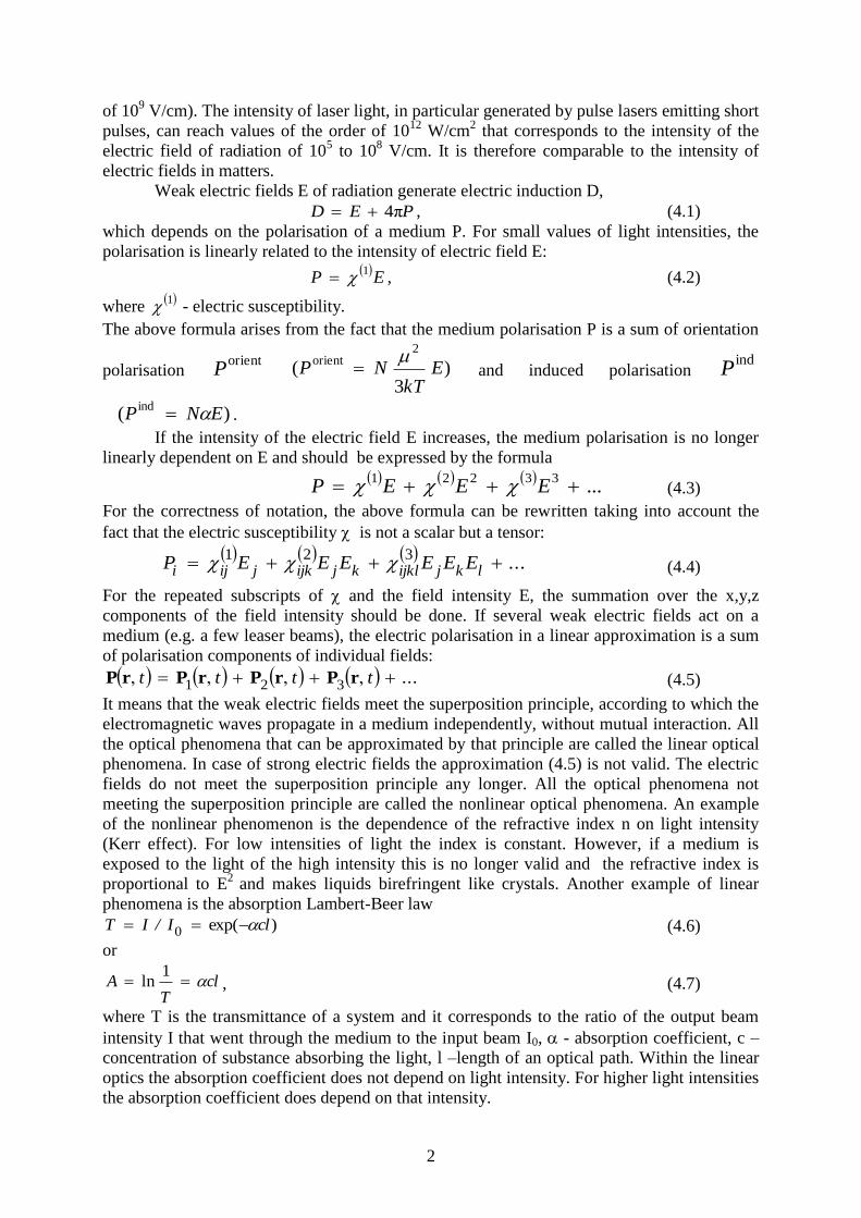
The second harmonic generation can be exemplified by the following experiment. Let

us direct a ruby laser light of the wavelength 694.3 nm on a nonlinear crystal. When we

rotate the crystal, one can notice that at a specific angle between the direction of laser beam

and the optical axis, the crystal output laser beam consists of two components: 694.3 nm and

694.3 nm/2 = 347.15 nm. Therefore, apart from the fundamental component 694.3 nm there

appears additional component, called the second harmonic of the frequency twice as high as

the fundamental (Fig. 4.3). The name of the process of the second harmonic generation can

also be abbreviated to SHG.

Fig. 4.1. Scheme of the second harmonic generation (SHG)

The second-order nonlinear phenomena are not so important in glass optical fibers. The silica

glasses in contrast to crystals have amorphous structure with the inversion center and do not

have the distinguished axis of symmetry. The inversion center simply means that the second –

order term (4.8) disappears and SHG do not occur in glass optical fibers. The detailed

description of the second-order nonlinear phenomena can be found in [4].

4.2. Third-order nonlinear phenomena [6]

One of the best known nonlinear optical phenomenon of the third-order is the

stimulated Raman scattering. Raman scattering processes can be expressed by the following

equation

lkjijklkjijkiji EEEEEEP 321 . (4.9)

The first term of the equation refers to the linear polarisation and depicts the spontaneous

linear Raman scattering. The second term express the spontaneous nonlinear Raman

scattering (hyperRaman scattering, HRS). The third term corresponds to the stimulated

Raman scattering.

4

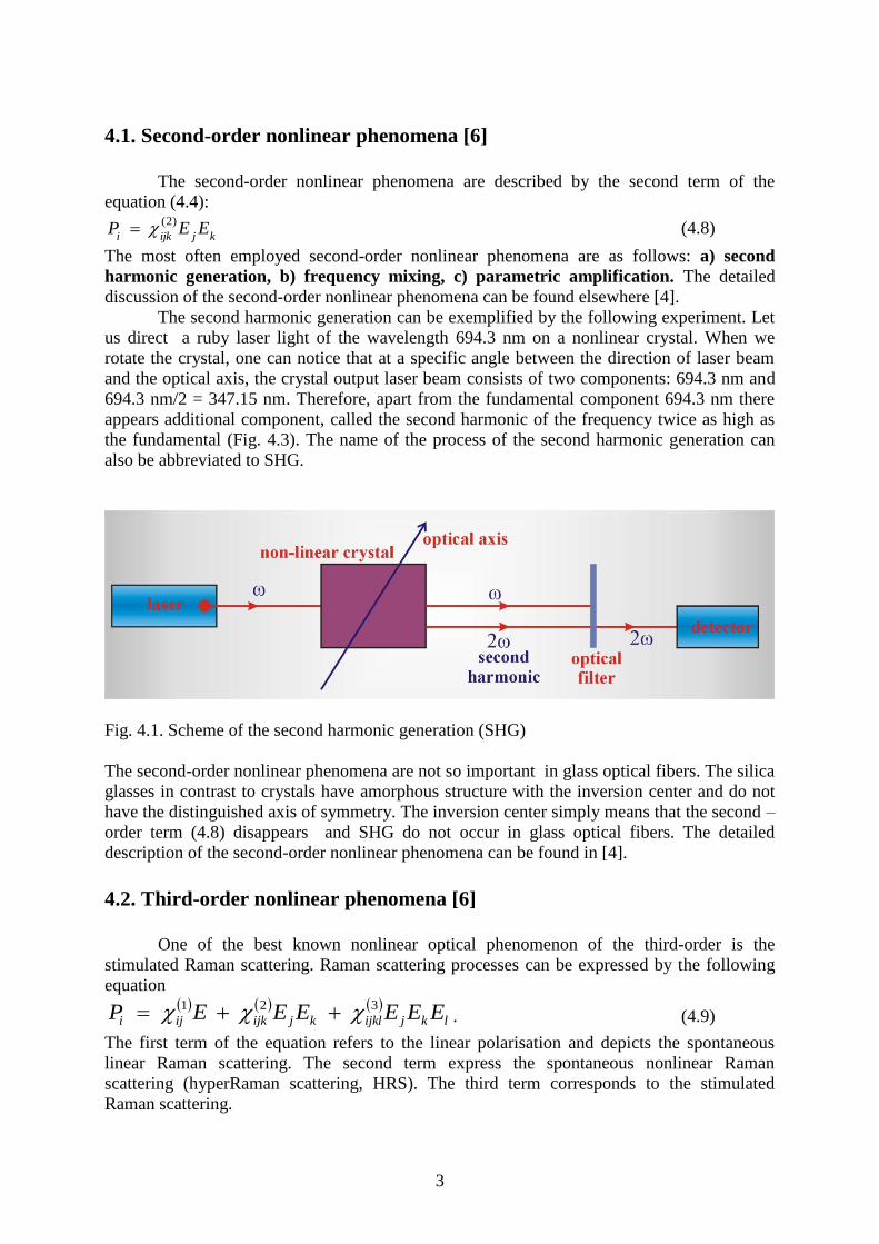
The spontaneous nonlinear Raman scattering has been described in a range of

textbooks. The spontaneous Raman scattering can be outlined according to the scheme

below(Fig. 4.2):

Fig. 4.2. Scheme of Rayleigh and Raman scattering.

E0 and E1 states correspond to the electronic states; the states enumerated with the quantum

numbers denote the vibration states. When a photon of light with energy of L

which is

lower than the resonance energy 01EEE , falls onto a molecule, it undergoes the

elastic or the inelastic scattering. The elastic scattering is called Rayleigh scattering, whereas

the inelastic scattering – Raman scattering. The scattering process can be described

classically. The electric field of the intensity tEL

rkcos0

produces the electron

polarisation P of a medium that is time-modulated with the frequency of L . Changeable

over time the polarisation of medium induces the emission of electromagnetic waves of the

same frequency L (when dipole vibration are not modulated by vibrations of a molecule of

the frequency wib

) or the frequency L wib

(if the vibrations of dipole are additionally

modulated by the vibrations of a molecule with the frequency of wib

). When the incident

and scattered radiation frequencies are the same and equal L , we call the phenomenon

Rayleigh scattering or elastic scattering. When the frequency of the scattered radiation is

lower )(wibL

or higher wibL

than the frequency of incident radiation L .

The scattered radiation of the frequency wibL

is called the Stokes Raman scattering

and that of the frequency wibL

- anti-Stokes Raman scattering.

Quantum description can also be applied for the Raman scattering processes. The

incident photon excites a molecule being in an electron state E0 and a ground vibrational state

( = 0) to a virtual state E that meets the condition 10 EEE . The lifetime of the

molecule being in the virtual state is very short and afterwards it turns to: a) the initial state

),( 00 E that is accompanied by the photon emission of L energy (Rayleigh

scattering), b) the excited vibration state ),( 10 E emitting photons of energy

5

wibL (Stokes Raman scattering) or c) if the photon irradiates a molecule in the

electronic state E0 and the excited vibration state = 1, then it returns to the ground state

),( 00 E that is accompanied by the emission of the energy photon, wibL (anti-

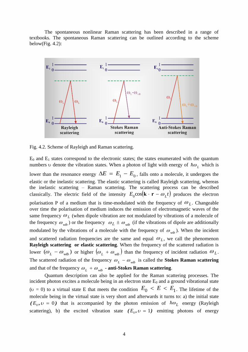
Stokes Raman scattering). When the intensity of the incident radiation increases, the

probability of the two photons Raman and Rayleigh scattering increases. Such phenomena are

known as hyperRaman or hyperRayleigh (Fig. 4.3) and they are described by the second term

of the (4.9).

Fig. 4.3. Hyper-Rayleigh and hyper-Raman scattering

4.3. Stimulated Raman scattering (SRS)

The above described processes belong to the group of spontaneous scattering

phenomena. Now, let us focus on the nonlinear third-order optical phenomena (3), which

are responsible for the stimulated Raman scattering (the third term in (4.9)).

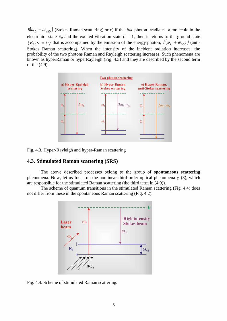
The scheme of quantum transitions in the stimulated Raman scattering (Fig. 4.4) does

not differ from these in the spontaneous Raman scattering (Fig. 4.2).

Fig. 4.4. Scheme of stimulated Raman scattering.

6

The difference is that the incident laser beam of the frequency L

characterised by the high

intensity generates a strong Stokes beam wibLs . As a result the Stokes beam

stimulates additional Stokes scattering from the virtual state E. This effect is analogous to the

spontaneous and stimulated emission in a laser. The main difference is that absorption,

spontaneous and stimulated emission occur between the stationary quantum states. For the

incident and the scattered light of high intensity, two beams - L and s

exist and interact

with molecules of the system. This interaction leads to the generation of the phase coherent

vibrations of the frequency sLwib . This denotes that all the molecules of the

system vibrate in the same phase of the frequency wib

, because the effects of inter- or

intramolecular interactions destroying the coherence are much lower than the strong

interaction of a molecule with the electric fields of the beams L

and s

.

The stimulated anti-Stokes scattering is generated in a similar way. The spontaneous

Raman scattering generates a weak anti-Stokes signal, since the population of the excited

vibration levels is low according to the Boltzmann distribution. Illumination of a system with

a high intensity L beam leads to a perturbation of the Bolzmann distribution and as a result

the stimulated anti-Stokes intensity increases significantly.

The stimulated Raman scattering is the special case of the four-wave interaction

3214 , (4.10)

04321 kkkkk . (4.11)

The equations (4.10) and (4.11) describe either three input 321

,, beams and one output

4 beam interaction or two-fold interaction of the same beam like in the case of the

stimulated Raman scattering. Indeed, the four-wave interaction for the stimulated Stokes

scattering can be written as follows

LLLLwibL)(

sss4 , (4.12)

thus, s4 ; L

1 ; s2

; L

3 . (4.13)

The intensity of the stimulated Stokes scattering, w

SI , can be expressed by the following

formula

2

2223

2

2

/kl

/kllIIAI L

sinS

w

S , (4.14)

where: A – a constant, LI and SI - the intensities of the incident (pumping) and Stokes

scattering beams, l – optical path length.

The anti-Stokes stimulated scattering can be written as a four-wave interaction

sAS

LLwibL , (4.15)

thus AS4 ;

L

1;

L

2;

S3 . (4.16)

The intensity of the stimulated anti-Stokes scattering, w

ASI , is expressed by the equation

2

2223

2

2

/kl

/kllIIAI L

sinS

w

AS . (4.17)

The expressions (4.14) and (4.17) do not differ in the form, however, one should notice that

the phase matching condition, k , varies for the Stokes and the anti-Stokes stimulated

7

scattering. The phase matching condition for the stimulated Stokes scattering takes the

following form (4.12)

0SLSLkkkkk , (4.18)

which indicates that the phase matching condition is satisfied for every propagation direction

of the stimulated Stokes scattering. It means that the phase matching between the pumping

beam, L , Stokes beam, s

, and vibrations is achieved automatically.

In case of the anti-Stokes scattering the phase matching condition takes the form

(4.15)

ASSASS2 kkkkkkkk

LLL . (4.19)

and the phase matching condition is only met for those directions that comply with the

relation

SAS2 kkk

L. (4.20)

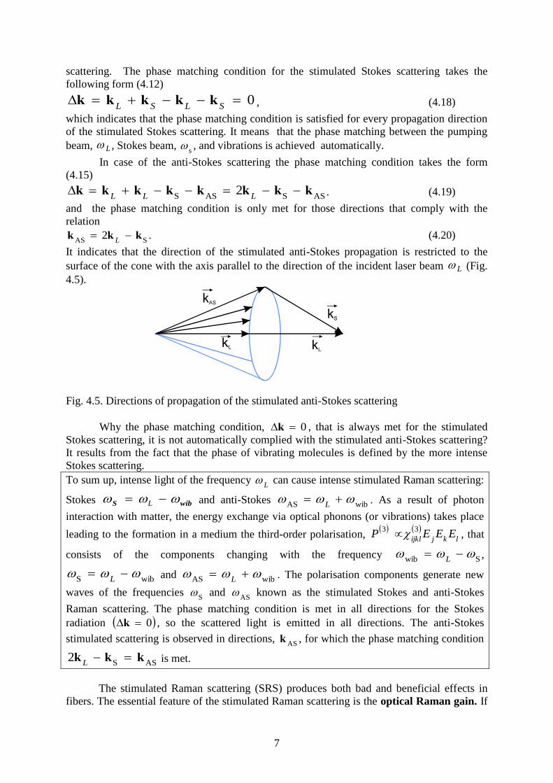
It indicates that the direction of the stimulated anti-Stokes propagation is restricted to the

surface of the cone with the axis parallel to the direction of the incident laser beam L (Fig.

4.5).

Fig. 4.5. Directions of propagation of the stimulated anti-Stokes scattering

Why the phase matching condition, 0k , that is always met for the stimulated

Stokes scattering, it is not automatically complied with the stimulated anti-Stokes scattering?

It results from the fact that the phase of vibrating molecules is defined by the more intense

Stokes scattering.

To sum up, intense light of the frequency L

can cause intense stimulated Raman scattering:

Stokes wibS L and anti-Stokes wibAS

L . As a result of photon

interaction with matter, the energy exchange via optical phonons (or vibrations) takes place

leading to the formation in a medium the third-order polarisation,

lkjijklEEEP

33 , that

consists of the components changing with the frequency Swib

L ,

wibS

L and wibAS

L . The polarisation components generate new

waves of the frequencies S

and AS

known as the stimulated Stokes and anti-Stokes

Raman scattering. The phase matching condition is met in all directions for the Stokes

radiation 0k , so the scattered light is emitted in all directions. The anti-Stokes

stimulated scattering is observed in directions, ASk , for which the phase matching condition

ASS2 kkk

L is met.

The stimulated Raman scattering (SRS) produces both bad and beneficial effects in

fibers. The essential feature of the stimulated Raman scattering is the optical Raman gain. If

8

in a medium, in which the stimulated Raman scattering occurs, two beams are guided: a beam

called pumping beam of L

frequency and the additional one of the lower frequency equals

to the Stokes component frequency wibS L (propagating signal beam) the latter

beam is significantly amplified. Therefore, we can expect the stimulated Raman scattering can

be employed to amplify the input signal pulse in an optical fiber in a similar way as it

undergoes in EDFAs, erbium-doped fibre amplifiers. The essential difference is the

amplification of the propagating beam via the stimulated Raman scattering and the

occurrence of the bathochromic shift (the Stokes component) vibl S with respect

to the pumping beam, where vib denotes vibration frequency of the molecules of the fiber

material (glass or dopants).

The Raman stimulated scattering in optical fiber can amplify weak propagating signal

of frequency s

if the intense light is simultaneously pumped into a fiber with the frequency

L corresponding the amplification Raman spectrum vibl S . Maximum of

amplification occurs only if the difference vibl S equals to the maximum of the

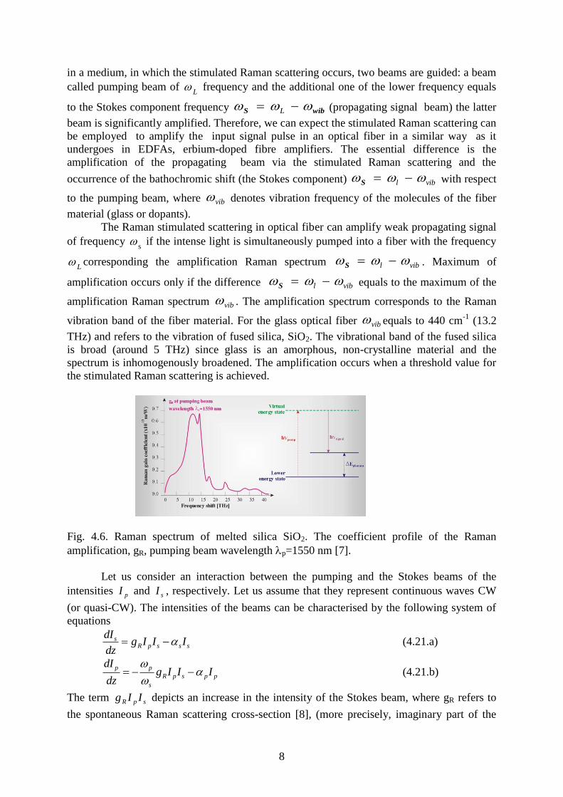
amplification Raman spectrum vib . The amplification spectrum corresponds to the Raman

vibration band of the fiber material. For the glass optical fiber vib equals to 440 cm-1

(13.2

THz) and refers to the vibration of fused silica, SiO2. The vibrational band of the fused silica

is broad (around 5 THz) since glass is an amorphous, non-crystalline material and the

spectrum is inhomogenously broadened. The amplification occurs when a threshold value for

the stimulated Raman scattering is achieved.

Fig. 4.6. Raman spectrum of melted silica SiO2. The coefficient profile of the Raman

amplification, gR, pumping beam wavelength p=1550 nm [7].

Let us consider an interaction between the pumping and the Stokes beams of the

intensities pI and sI , respectively. Let us assume that they represent continuous waves CW

(or quasi-CW). The intensities of the beams can be characterised by the following system of

equations

ssspRs IIIg

dz

dI (4.21.a)

ppspR

s

ppIIIg

dz

dI

(4.21.b)

The term spR IIg depicts an increase in the intensity of the Stokes beam, where gR refers to

the spontaneous Raman scattering cross-section [8], (more precisely, imaginary part of the

9

third-order electric susceptibility 3

ijkl in the equation (4.9)), s p - coefficients describing

loses in an optical fiber for the Stokes and the pumping beams. One can accurately derive the

equations (4.21.a - 4.21.b) from the Maxwell equations but they can also be intuitively

understood as phenomenological equations. It becomes particularly clear for the case when

the loses in the equation (4.21.b) are neglected, then we can write

0

p

p

s

s

z

II

d

d

(4.22)

This equation states that the total number of photons remains constant in the process of SRS.

In order to achieve the pumping beam pI intensity threshold value, the set of equations

(4.21.a - 4.21.b) has to be solved. To simplify the case, let us neglect the first term in the

equation (4.21.b)

pp

z

pI

d

dI (4.23)

Solving the equation (4.23) and inserting to the equation (4.21a) we obtain

SSSpRz II)zexp(Ig

dz

dI 0 (4.24)

where 0I denotes the intensity of pumping beam at the input, for z=0.

Solving the equation (4.24) we get

LLIgexpILI seffRss 00 (4.25)

where L denotes the length of an optical fiber, while effL is an effective length of an optical

fiber

p

p

eff

LexpL

1 (4.26)

The equation (4.25) says that at (z=0) where the pumping beam is injected the intensity of

the signal beam is equal 0sI and as a result of the stimulated Raman scattering is amplified

to the value LI s when propagating along the length L. Here we assumed that during the

process of SRS the photons of the frequency are generated. Indeed, SRS process amplifies

all signals of the frequencies from the Raman band range (Fig. 4.6). Therefore the equation

(4.25) should be substituted by the integration over whole Raman amplification band.

dLLIgexpLP seffpRs

0 (4.27)

In order to solve the equation (4.27) the specific form of )(gg RR has to be known,

where p . Since usually the relation is not known, )(gg RR has to be

expanded into Taylor series around the Stokes frequency S and after substitution of

the expansion we obtain

LLIgexpPLP seffRR

eff

ss 00 (4.28)

where

effs

eff

s BP 0 (4.29)

2

1

2

22

1

0

2

s

R

eff

eff

g

LIB

(4.30)

10

effB has the meaning of the effective Stokes bandwidth, and depends also on the pumping

intensity and the fiber length L. The expression (4.29) can be treated as a good first-order

approximation for estimation of the threshold power eff

sP 0 , which is defined as the power of

the Stokes beam power equal to the pumping power at the end of a fiber of the length L.

LexpPLPLP pps 0 (4.31)

where effAIP 00 while effA denotes the effective surface of the optical fiber core defined

by the equation:

dxdyy,xF

dxdyy,xF

Aeff4

22

(4.32)

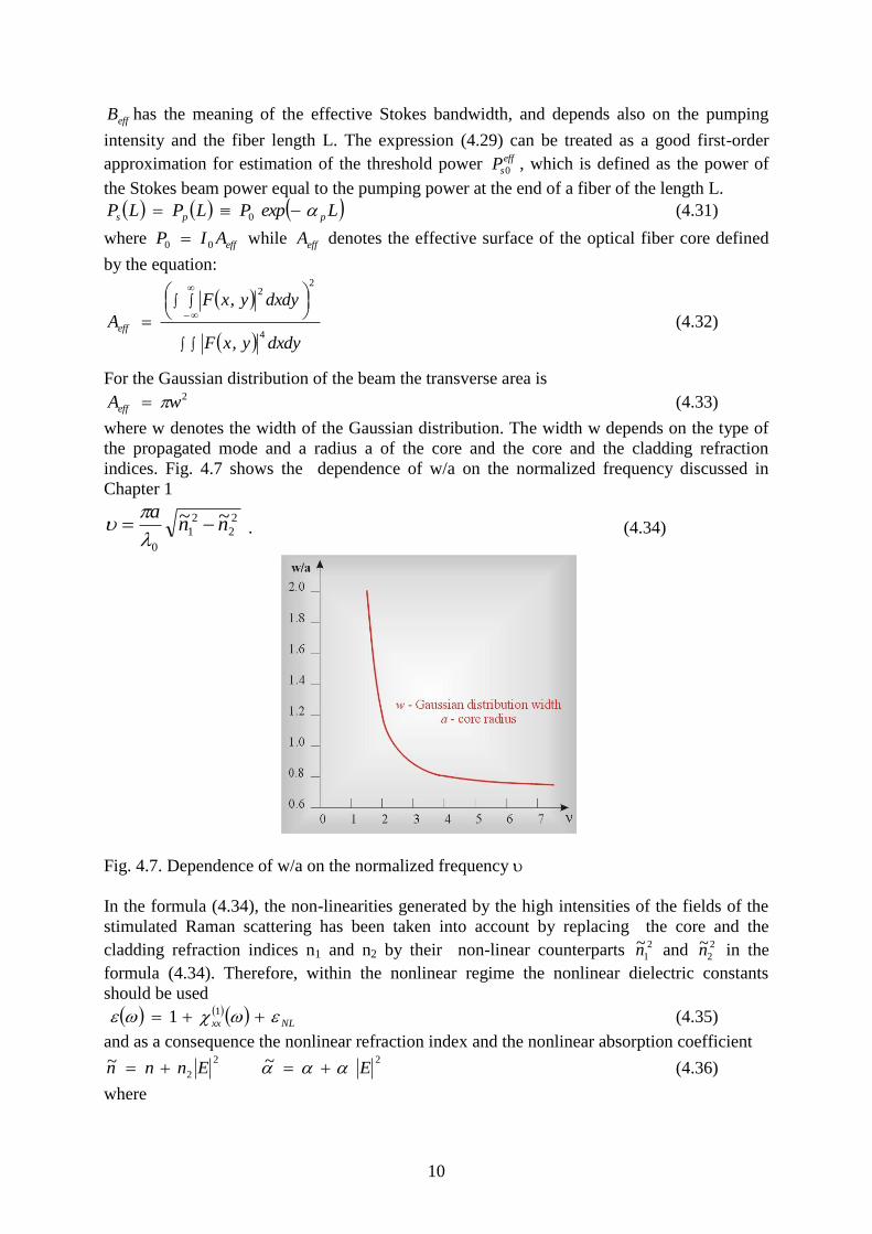
For the Gaussian distribution of the beam the transverse area is 2wAeff (4.33)

where w denotes the width of the Gaussian distribution. The width w depends on the type of

the propagated mode and a radius a of the core and the core and the cladding refraction

indices. Fig. 4.7 shows the dependence of w/a on the normalized frequency discussed in

Chapter 1

2

2

2

1

0

~~ nna

. (4.34)

Fig. 4.7. Dependence of w/a on the normalized frequency

In the formula (4.34), the non-linearities generated by the high intensities of the fields of the

stimulated Raman scattering has been taken into account by replacing the core and the

cladding refraction indices n1 and n2 by their non-linear counterparts 2

1~n and 2

2~n in the

formula (4.34). Therefore, within the nonlinear regime the nonlinear dielectric constants

should be used

NLxx 11 (4.35)

and as a consequence the nonlinear refraction index and the nonlinear absorption coefficient 2

2 Ennn~ 2

E~ (4.36)

where

11

3

28

3xxxxRe

nn , 30

24

3xxxxIm

nc

(4.37)

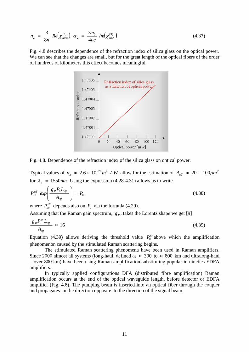
Fig. 4.8 describes the dependence of the refraction index of silica glass on the optical power.

We can see that the changes are small, but for the great length of the optical fibers of the order

of hundreds of kilometers this effect becomes meaningful.

Fig. 4.8. Dependence of the refraction index of the silica glass on optical power.

Typical values of W/m.n 220

2 1062 allow for the estimation of 210020 mAeff

for nmp 1550 . Using the expression (4.28-4.31) allows us to write

0

0

0 PA

LPgexpP

eff

effReff

s

(4.38)

where eff

sP 0 depends also on 0P via the formula (4.29).

Assuming that the Raman gain spectrum, Rg , takes the Lorentz shape we get [9]

160

eff

eff

cr

R

A

LPg (4.39)

Equation (4.39) allows deriving the threshold value crP0 above which the amplification

phenomenon caused by the stimulated Raman scattering begins.

The stimulated Raman scattering phenomena have been used in Raman amplifiers.

Since 2000 almost all systems (long-haul, defined as 300 to 800 km and ultralong-haul

– over 800 km) have been using Raman amplification substituting popular in nineties EDFA

amplifiers.

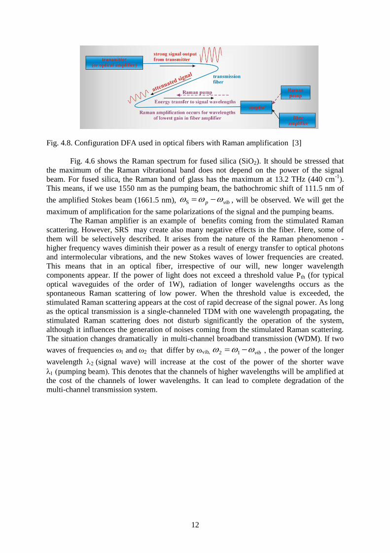
In typically applied configurations DFA (distributed fibre amplification) Raman

amplification occurs at the end of the optical waveguide length, before detector or EDFA

amplifier (Fig. 4.8). The pumping beam is inserted into an optical fiber through the coupler

and propagates in the direction opposite to the direction of the signal beam.

12

Fig. 4.8. Configuration DFA used in optical fibers with Raman amplification [3]

Fig. 4.6 shows the Raman spectrum for fused silica (SiO2). It should be stressed that

the maximum of the Raman vibrational band does not depend on the power of the signal

beam. For fused silica, the Raman band of glass has the maximum at 13.2 THz (440 cm-1

).

This means, if we use 1550 nm as the pumping beam, the bathochromic shift of 111.5 nm of

the amplified Stokes beam (1661.5 nm), vibp S , will be observed. We will get the

maximum of amplification for the same polarizations of the signal and the pumping beams.

The Raman amplifier is an example of benefits coming from the stimulated Raman

scattering. However, SRS may create also many negative effects in the fiber. Here, some of

them will be selectively described. It arises from the nature of the Raman phenomenon -

higher frequency waves diminish their power as a result of energy transfer to optical photons

and intermolecular vibrations, and the new Stokes waves of lower frequencies are created.

This means that in an optical fiber, irrespective of our will, new longer wavelength

components appear. If the power of light does not exceed a threshold value Pth (for typical

optical waveguides of the order of 1W), radiation of longer wavelengths occurs as the

spontaneous Raman scattering of low power. When the threshold value is exceeded, the

stimulated Raman scattering appears at the cost of rapid decrease of the signal power. As long

as the optical transmission is a single-channeled TDM with one wavelength propagating, the

stimulated Raman scattering does not disturb significantly the operation of the system,

although it influences the generation of noises coming from the stimulated Raman scattering.

The situation changes dramatically in multi-channel broadband transmission (WDM). If two

waves of frequencies andthatdiffer by vib vib 12 the power of the longer

wavelength (signal wave) will increase at the cost of the power of the shorter wave

pumping beam. This denotes that the channels of higher wavelengths will be amplified at

the cost of the channels of lower wavelengths. It can lead to complete degradation of the

multi-channel transmission system.

13

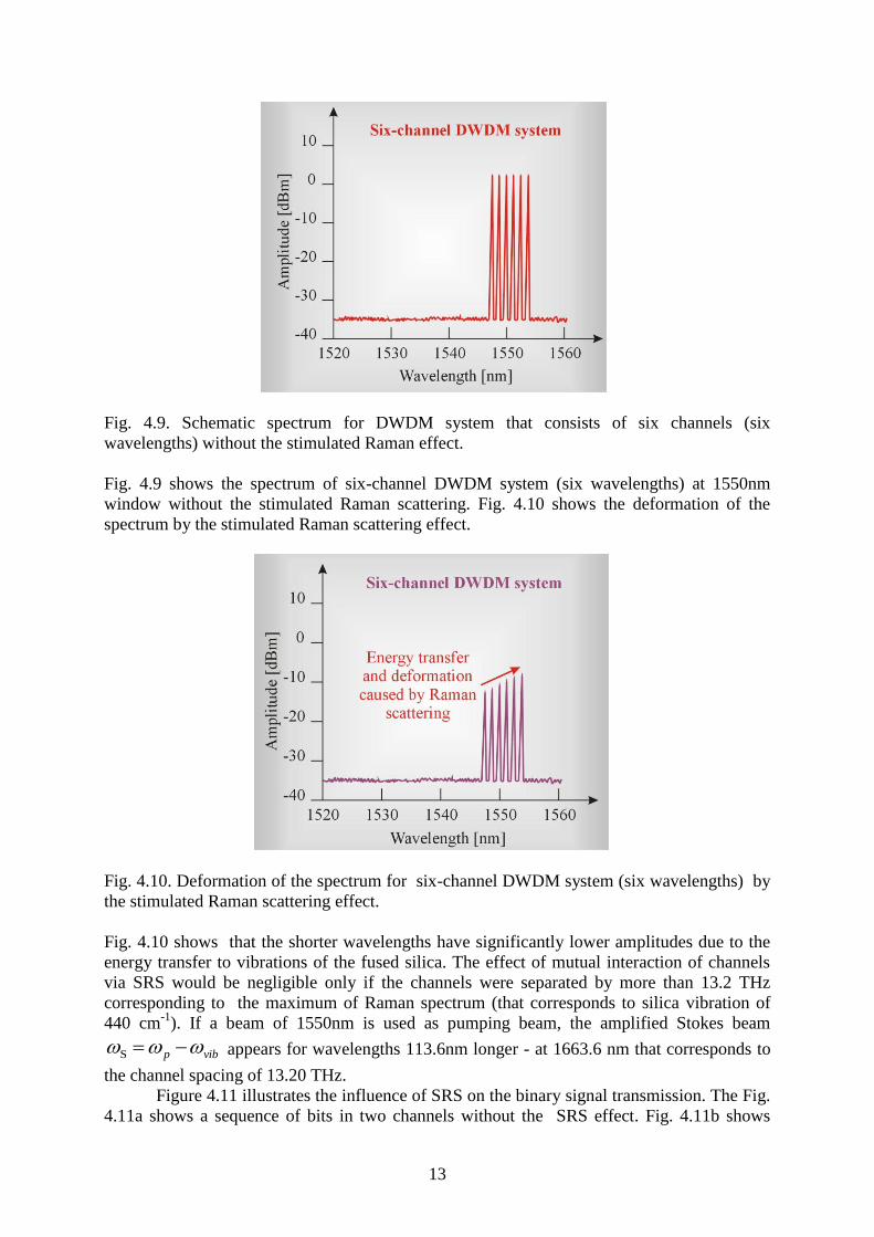
Fig. 4.9. Schematic spectrum for DWDM system that consists of six channels (six

wavelengths) without the stimulated Raman effect.

Fig. 4.9 shows the spectrum of six-channel DWDM system (six wavelengths) at 1550nm

window without the stimulated Raman scattering. Fig. 4.10 shows the deformation of the

spectrum by the stimulated Raman scattering effect.

Fig. 4.10. Deformation of the spectrum for six-channel DWDM system (six wavelengths) by

the stimulated Raman scattering effect.

Fig. 4.10 shows that the shorter wavelengths have significantly lower amplitudes due to the

energy transfer to vibrations of the fused silica. The effect of mutual interaction of channels

via SRS would be negligible only if the channels were separated by more than 13.2 THz

corresponding to the maximum of Raman spectrum (that corresponds to silica vibration of

440 cm-1

). If a beam of 1550nm is used as pumping beam, the amplified Stokes beam

vibp S appears for wavelengths 113.6nm longer - at 1663.6 nm that corresponds to

the channel spacing of 13.20 THz.

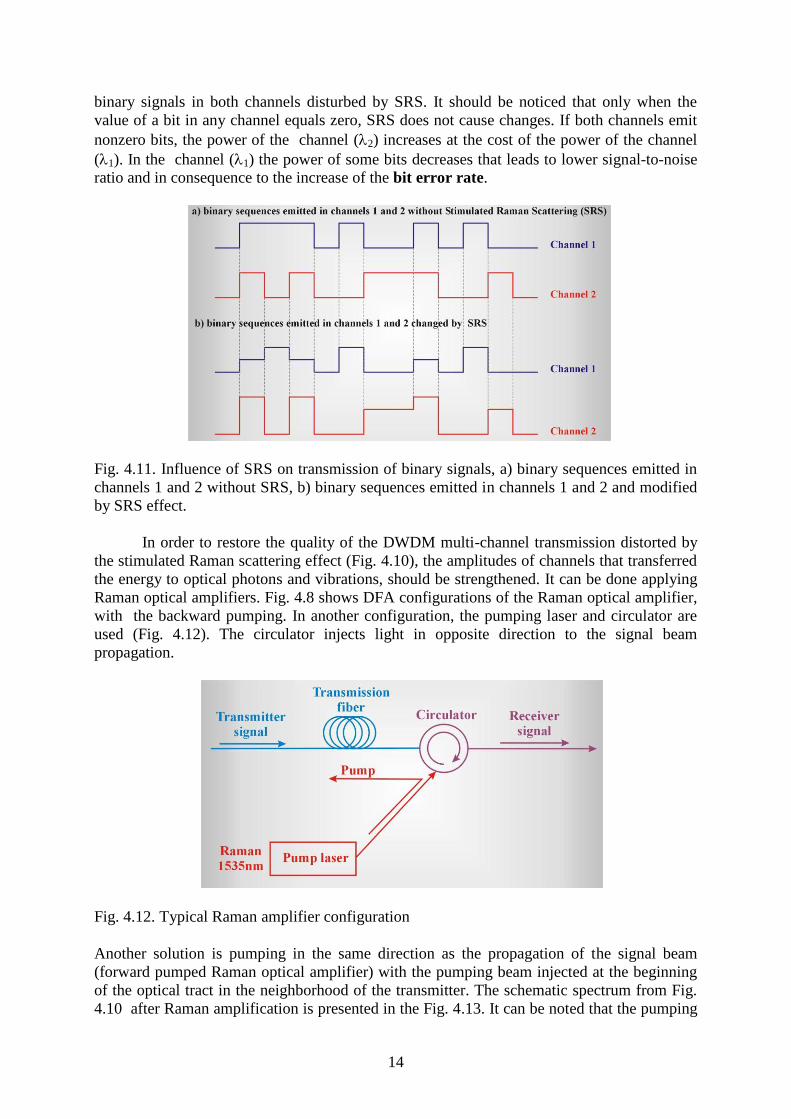
Figure 4.11 illustrates the influence of SRS on the binary signal transmission. The Fig.

4.11a shows a sequence of bits in two channels without the SRS effect. Fig. 4.11b shows

14

binary signals in both channels disturbed by SRS. It should be noticed that only when the

value of a bit in any channel equals zero, SRS does not cause changes. If both channels emit

nonzero bits, the power of the channel (2) increases at the cost of the power of the channel

(1). In the channel (1) the power of some bits decreases that leads to lower signal-to-noise

ratio and in consequence to the increase of the bit error rate.

Fig. 4.11. Influence of SRS on transmission of binary signals, a) binary sequences emitted in

channels 1 and 2 without SRS, b) binary sequences emitted in channels 1 and 2 and modified

by SRS effect.

In order to restore the quality of the DWDM multi-channel transmission distorted by

the stimulated Raman scattering effect (Fig. 4.10), the amplitudes of channels that transferred

the energy to optical photons and vibrations, should be strengthened. It can be done applying

Raman optical amplifiers. Fig. 4.8 shows DFA configurations of the Raman optical amplifier,

with the backward pumping. In another configuration, the pumping laser and circulator are

used (Fig. 4.12). The circulator injects light in opposite direction to the signal beam

propagation.

Fig. 4.12. Typical Raman amplifier configuration

Another solution is pumping in the same direction as the propagation of the signal beam

(forward pumped Raman optical amplifier) with the pumping beam injected at the beginning

of the optical tract in the neighborhood of the transmitter. The schematic spectrum from Fig.

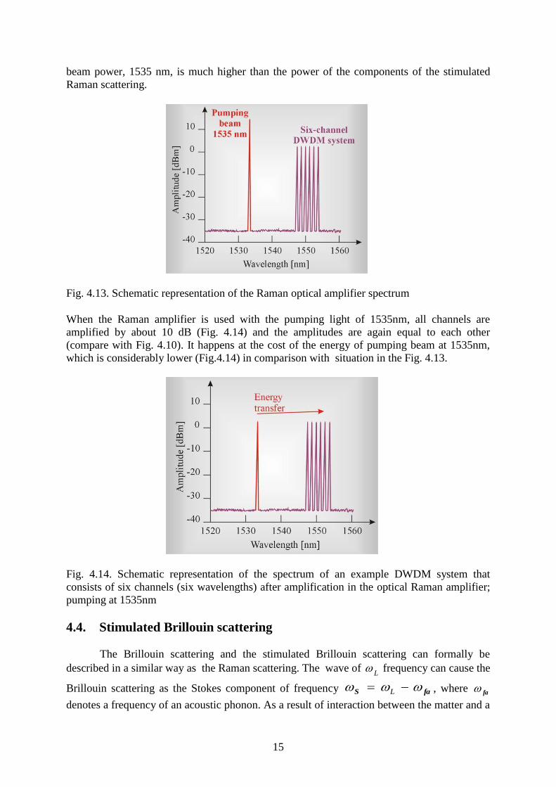
4.10 after Raman amplification is presented in the Fig. 4.13. It can be noted that the pumping

15

beam power, 1535 nm, is much higher than the power of the components of the stimulated

Raman scattering.

Fig. 4.13. Schematic representation of the Raman optical amplifier spectrum

When the Raman amplifier is used with the pumping light of 1535nm, all channels are

amplified by about 10 dB (Fig. 4.14) and the amplitudes are again equal to each other

(compare with Fig. 4.10). It happens at the cost of the energy of pumping beam at 1535nm,

which is considerably lower (Fig.4.14) in comparison with situation in the Fig. 4.13.

Fig. 4.14. Schematic representation of the spectrum of an example DWDM system that

consists of six channels (six wavelengths) after amplification in the optical Raman amplifier;

pumping at 1535nm

4.4. Stimulated Brillouin scattering

The Brillouin scattering and the stimulated Brillouin scattering can formally be

described in a similar way as the Raman scattering. The wave of L

frequency can cause the

Brillouin scattering as the Stokes component of frequency faS L , where fa

denotes a frequency of an acoustic phonon. As a result of interaction between the matter and a

16

light photons the energy exchange occurs via acoustic photons leading to the third-order

polarization of in medium,

lkjijklEEEP

33 . The fundamental difference lies in the

interaction of light photons with acoustic phonons in contrast to the Raman scattering where

the interactions between light photons and molecular vibrations occur. The acoustic phonons

are of much lower frequencies than optical photons. The frequency of the acoustic phonon is

expressed by the following formula

s

fa

n4 (4.40)

where s denotes the speed of sound in optical waveguide, n – refraction index. One can

estimate the typical acoustic frequency from (4.40) which is equals to 69 GHz at wavelength

of 1550nm.

The Brillouin scattering becomes the stimulated Brillouin scattering when the

pumping threshold value is exceeded to generate the Stokes amplification. The bandwidth of

the Brillouin amplification is much narrower than that of the Raman band and is equal

approximately around B =20 MHz for 1550 nm. For comparison, the Raman amplification

band is broad and equals around 5THz. This means that the highest amplification (the lowest

threshold value) occurs for the sources of spectral bandwidth smaller than 20MHz. Indeed, the

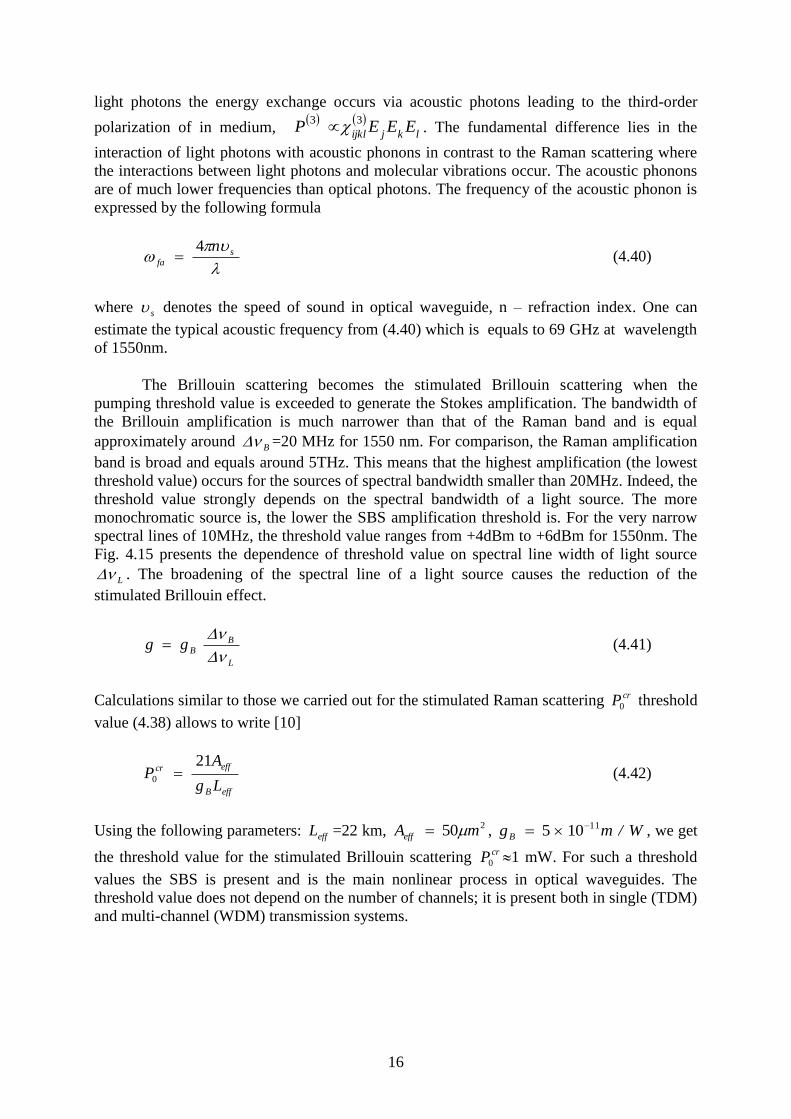
threshold value strongly depends on the spectral bandwidth of a light source. The more

monochromatic source is, the lower the SBS amplification threshold is. For the very narrow

spectral lines of 10MHz, the threshold value ranges from +4dBm to +6dBm for 1550nm. The

Fig. 4.15 presents the dependence of threshold value on spectral line width of light source

L . The broadening of the spectral line of a light source causes the reduction of the

stimulated Brillouin effect.

L

BBgg

(4.41)

Calculations similar to those we carried out for the stimulated Raman scattering crP0 threshold

value (4.38) allows to write [10]

effB

effcr

Lg

AP

210 (4.42)

Using the following parameters: effL =22 km, 250 mAeff , W/mgB

11105 , we get

the threshold value for the stimulated Brillouin scattering crP0 1 mW. For such a threshold

values the SBS is present and is the main nonlinear process in optical waveguides. The

threshold value does not depend on the number of channels; it is present both in single (TDM)

and multi-channel (WDM) transmission systems.

17

Fig. 4.15. The dependence of the threshold value on spectral line width.

Although the mechanisms of simulated Raman and Brillouin scattering are formally similar,

there exist a few fundamental differences. First, the scattering amplification coefficient,

W/cmgB

9104 , is twice as high as the corresponding coefficient for Raman

scattering. It means a power of a few mW is enough for SBS effect production contrary to

SRS where a power of above 200 mW causes SRS amplification. Second, contrary to Raman

scattering, which propagates in both directions in an optical waveguide, Brillouin scattering

propagates only in reverse direction in single-mode optical waveguides. Reverse process of

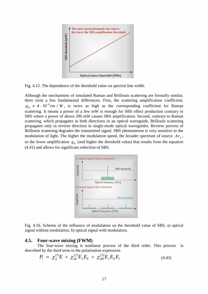
Brillouin scattering degrades the transmitted signal. SBS phenomenon is very sensitive to the

modulation of light. The higher the modulation speed, the broader spectrum of source L ,

so the lower amplification Bg (and higher the threshold value) that results from the equation

(4.41) and allows for significant reduction of SBS.

Fig. 4.16. Scheme of the influence of modulation on the threshold value of SBS, a) optical

signal without modulation, b) optical signal with modulation.

4.5. Four-wave mixing (FWM) The four-wave mixing is nonlinear process of the third order. This process is

described by the third term in the polarisation expression

lkjijklkjijkiji EEEEEEP 321 (4.43)

18

As it has been shown in the chapter 3, the stimulated Raman scattering can be regarded as a

special case of four-wave interaction

3214 (4.44)

04321 kkkkk

Also the third harmonic generation is a special case of FWM, which appears when

321 (4.45)

and we obtain

11114 3 . (4.46)

In case of the single-channel optical transmission, the generation of the III harmonic is

not a problem, since this nonlinear component can easily be filtrated, because it is in the

spectral region significantly distant from the transmitted signal of 1 frequency. However, in

the multi-channel systems with slightly different channel frequencies, the four-wave mixing

leads to various combinations and some of them precisely overlap with the signal beam and

the filtration becomes impossible. It is clear that the four-wave mixing is disadvantageous in

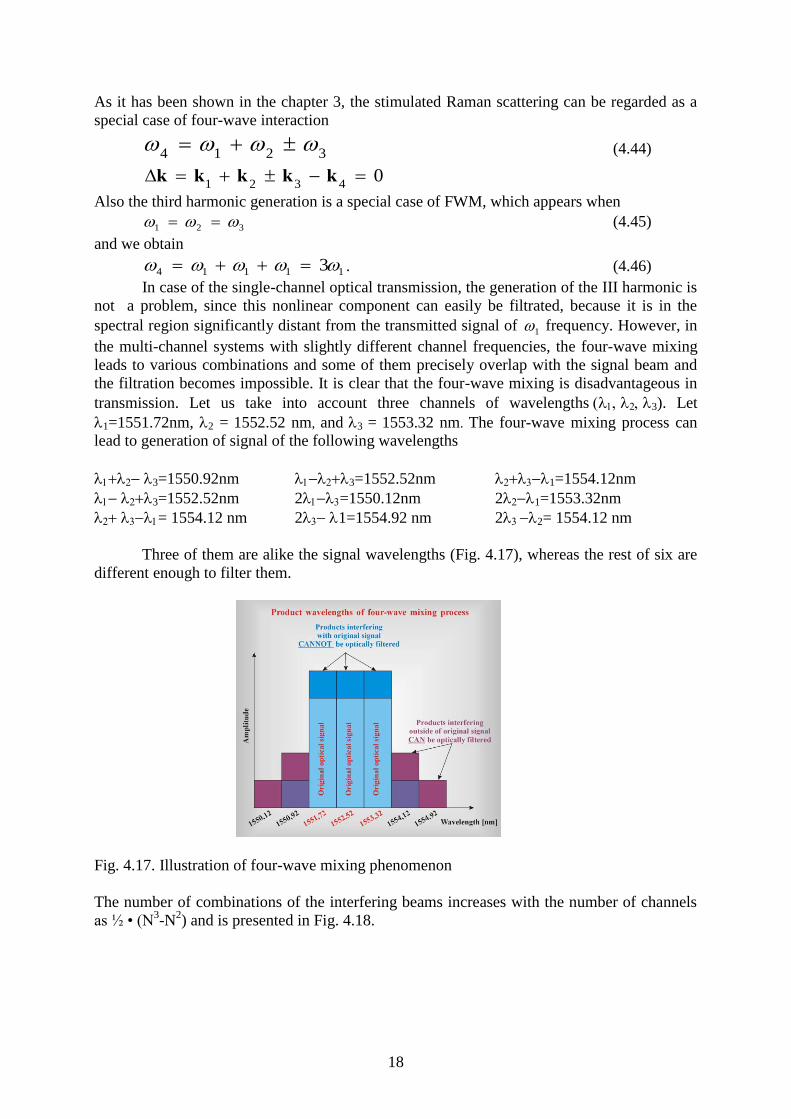
transmission. Let us take into account three channels of wavelengths3). Let

1=1551.72nm, 2 = 1552.52 nm, and 3 = 1553.32 nm. The four-wave mixing process can

lead to generation of signal of the following wavelengths

3=1550.92nm

3=1552.52nm

= 1554.12 nm

3=1552.52nm

2=1550.12nm

21=1554.92 nm

1=1554.12nm

21=1553.32nm

22= 1554.12 nm

Three of them are alike the signal wavelengths (Fig. 4.17), whereas the rest of six are

different enough to filter them.

Fig. 4.17. Illustration of four-wave mixing phenomenon

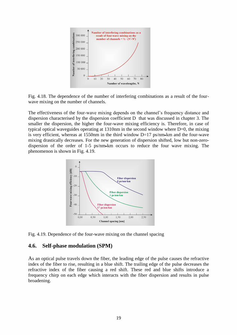
The number of combinations of the interfering beams increases with the number of channels

as ½ • (N3-N

2) and is presented in Fig. 4.18.

19

Fig. 4.18. The dependence of the number of interfering combinations as a result of the four-

wave mixing on the number of channels.

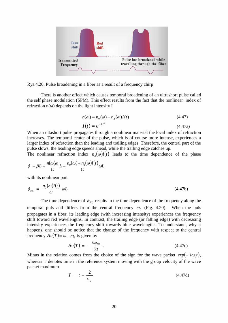
The effectiveness of the four-wave mixing depends on the channel’s frequency distance and

dispersion characterised by the dispersion coefficient D that was discussed in chapter 3. The

smaller the dispersion, the higher the four-wave mixing efficiency is. Therefore, in case of

typical optical waveguides operating at 1310nm in the second window where D=0, the mixing

is very efficient, whereas at 1550nm in the third window D=17 ps/nmkm and the four-wave

mixing drastically decreases. For the new generation of dispersion shifted, low but non-zero-

dispersion of the order of 1-5 ps/nmkm occurs to reduce the four wave mixing. The

phenomenon is shown in Fig. 4.19.

Fig. 4.19. Dependence of the four-wave mixing on the channel spacing

4.6. Self-phase modulation (SPM)

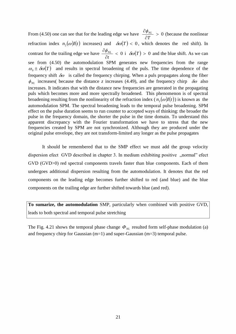
As an optical pulse travels down the fiber, the leading edge of the pulse causes the refractive

index of the fiber to rise, resulting in a blue shift. The trailing edge of the pulse decreases the

refractive index of the fiber causing a red shift. These red and blue shifts introduce a

frequency chirp on each edge which interacts with the fiber dispersion and results in pulse

broadening.

20

Rys.4.20. Pulse broadening in a fiber as a result of a frequency chirp

There is another effect which causes temporal broadening of an ultrashort pulse called

the self phase modulation (SPM). This effect results from the fact that the nonlinear index of

refraction n() depends on the light intensity I

)()()()( 20 tInnn (4.47) 2

)( tetI (4.47a)

When an ultashort pulse propagates through a nonlinear material the local index of refraction

increases. The temporal center of the pulse, which is of course more intense, experiences a

larger index of refraction than the leading and trailing edges. Therefore, the central part of the

pulse slows, the leading edge speeds ahead, while the trailing edge catches up.

The nonlinear refraction index tIn 2 leads to the time dependence of the phase

L

C

tInnL

C

nL

20

with its nonlinear part

L

C

tInNL

2 (4.47b)

The time dependence of NL results in the time dependence of the frequency along the

temporal puls and differs from the central frequency 0 (Fig. 4.20). When the puls

propagates in a fiber, its leading edge (with increasing intensity) experiences the frequency

shift toward red wavelengths. In contrast, the trailing edge (or falling edge) with decreasing

intensity experiences the frequency shift towards blue wavelengths. To understand, why it

happens, one should be notice that the change of the frequency with respect to the central

frequency 0 T is given by

T

T NL

. (4.47c)

Minus in the relation comes from the choice of the sign for the wave packet tiexp 0 ,

whereas T denotes time in the reference system moving with the group velocity of the wave

packet maximum

g

tT

2 (4.47d)

21

From (4.50) one can see that for the leading edge we have 0

T

NL (because the nonlinear

refraction index tIn 2 increases) and 0T , which denotes the red shift). In

contrast for the trailing edge we have 0

t

NL i 0T and the blue shift. As we can

see from (4.50) the automodulation SPM generates new frequencies from the range

0 T and results in spectral broadening of the puls. The time dependence of the

frequency shift is called the frequency chirping. When a puls propagates along the fiber

NL increases( because the distance z increases (4.49), and the frequency chirp also

increases. It indicates that with the distance new frequencies are generated in the propagating

puls which becomes more and more spectrally broadened. This phenomenon is of spectral

broadening resulting from the nonlinearity of the refraction index ( tIn 2 ) is known as the

automodulation SPM. The spectral broadening leads to the temporal pulse broadening. SPM

effect on the pulse duration seems to run counter to accepted ways of thinking: the broader the

pulse in the frequency domain, the shorter the pulse in the time domain. To understand this

apparent discrepancy with the Fourier transformation we have to stress that the new

frequencies created by SPM are not synchronized. Although they are produced under the

original pulse envelope, they are not transform-limited any longer as the pulse propagates

It should be remembered that to the SMP effect we must add the group velocity

dispersion efect GVD described in chapter 3. In medium exhibiting positive „normal” efect

GVD (GVD>0) red spectral components travels faster than blue components. Each of them

undergoes additional dispersion resulting from the automodulation. It denotes that the red

components on the leading edge becomes further shifted to red (and blue) and the blue

components on the trailing edge are further shifted towards blue (and red).

To sumarize, the automodulation SMP, particularly when combined with positive GVD,

leads to both spectral and temporal pulse stretching

The Fig. 4.21 shows the temporal phase change NL resulted form self-phase modulation (a)

and frequency chirp for Gaussian (m=1) and super-Gaussian (m=3) temporal pulse.

22

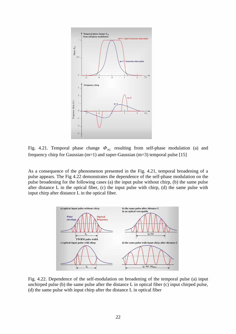
Fig. 4.21. Temporal phase change NL resulting from self-phase modulation (a) and

frequency chirp for Gaussian (m=1) and super-Gaussian (m=3) temporal pulse [15]

As a consequence of the phenomenon presented in the Fig. 4.21, temporal broadening of a

pulse appears. The Fig 4.22 demonstrates the dependence of the self-phase modulation on the

pulse broadening for the following cases (a) the input pulse without chirp, (b) the same pulse

after distance L in the optical fiber, (c) the input pulse with chirp, (d) the same pulse with

input chirp after distance L in the optical fiber.

Fig. 4.22. Dependence of the self-modulation on broadening of the temporal pulse (a) input

unchirped pulse (b) the same pulse after the distance L in optical fiber (c) input chirped pulse,

(d) the same pulse with input chirp after the distance L in optical fiber

23

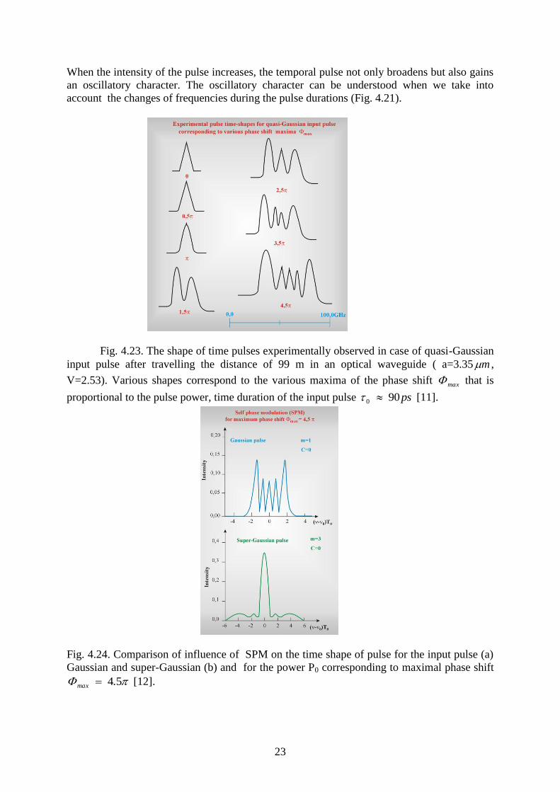
When the intensity of the pulse increases, the temporal pulse not only broadens but also gains

an oscillatory character. The oscillatory character can be understood when we take into

account the changes of frequencies during the pulse durations (Fig. 4.21).

Fig. 4.23. The shape of time pulses experimentally observed in case of quasi-Gaussian

input pulse after travelling the distance of 99 m in an optical waveguide ( a=3.35 m ,

V=2.53). Various shapes correspond to the various maxima of the phase shift max that is

proportional to the pulse power, time duration of the input pulse ps900 [11].

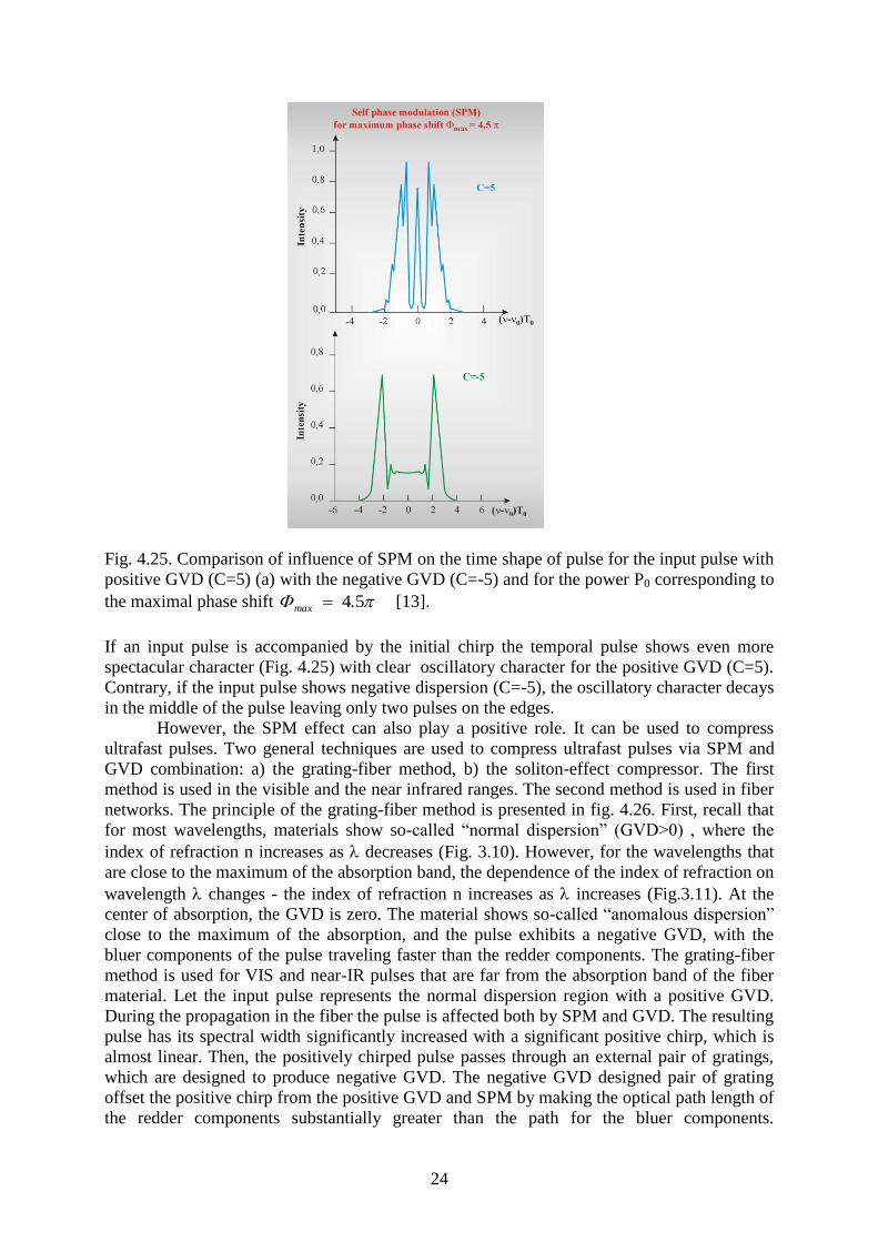
Fig. 4.24. Comparison of influence of SPM on the time shape of pulse for the input pulse (a)

Gaussian and super-Gaussian (b) and for the power P0 corresponding to maximal phase shift

54.max [12].

24

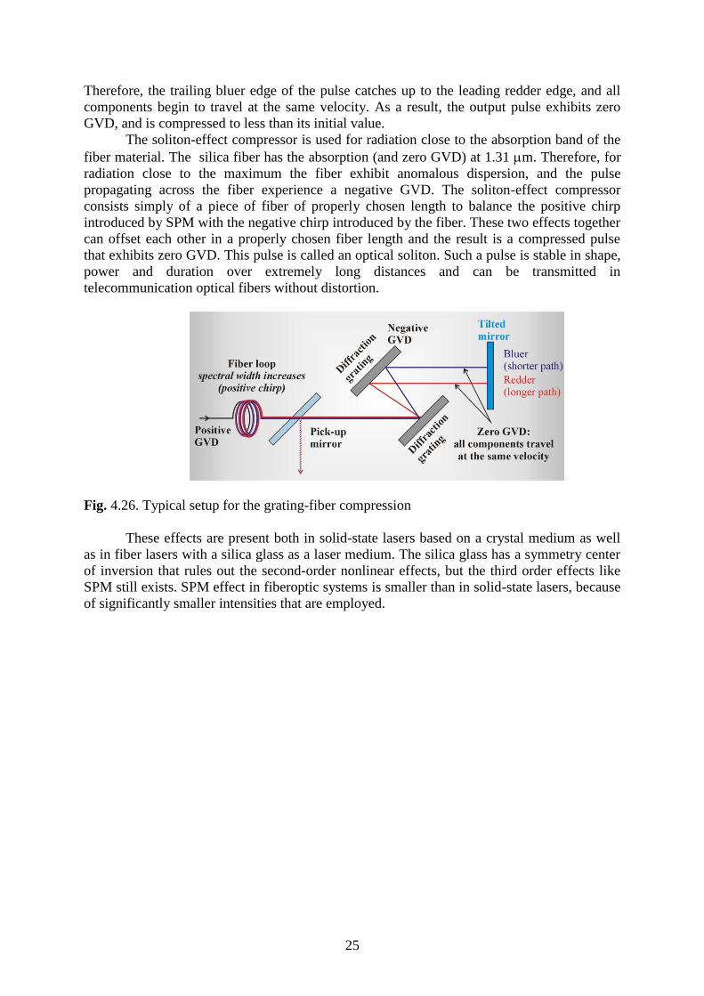
Fig. 4.25. Comparison of influence of SPM on the time shape of pulse for the input pulse with

positive GVD (C=5) (a) with the negative GVD (C=-5) and for the power P0 corresponding to

the maximal phase shift 54.max [13].

If an input pulse is accompanied by the initial chirp the temporal pulse shows even more

spectacular character (Fig. 4.25) with clear oscillatory character for the positive GVD (C=5).

Contrary, if the input pulse shows negative dispersion (C=-5), the oscillatory character decays

in the middle of the pulse leaving only two pulses on the edges.

However, the SPM effect can also play a positive role. It can be used to compress

ultrafast pulses. Two general techniques are used to compress ultrafast pulses via SPM and

GVD combination: a) the grating-fiber method, b) the soliton-effect compressor. The first

method is used in the visible and the near infrared ranges. The second method is used in fiber

networks. The principle of the grating-fiber method is presented in fig. 4.26. First, recall that

for most wavelengths, materials show so-called “normal dispersion” (GVD>0) , where the

index of refraction n increases as decreases (Fig. 3.10). However, for the wavelengths that

are close to the maximum of the absorption band, the dependence of the index of refraction on

wavelength changes - the index of refraction n increases as increases (Fig.3.11). At the

center of absorption, the GVD is zero. The material shows so-called “anomalous dispersion”

close to the maximum of the absorption, and the pulse exhibits a negative GVD, with the

bluer components of the pulse traveling faster than the redder components. The grating-fiber

method is used for VIS and near-IR pulses that are far from the absorption band of the fiber

material. Let the input pulse represents the normal dispersion region with a positive GVD.

During the propagation in the fiber the pulse is affected both by SPM and GVD. The resulting

pulse has its spectral width significantly increased with a significant positive chirp, which is

almost linear. Then, the positively chirped pulse passes through an external pair of gratings,

which are designed to produce negative GVD. The negative GVD designed pair of grating

offset the positive chirp from the positive GVD and SPM by making the optical path length of

the redder components substantially greater than the path for the bluer components.

25

Therefore, the trailing bluer edge of the pulse catches up to the leading redder edge, and all

components begin to travel at the same velocity. As a result, the output pulse exhibits zero

GVD, and is compressed to less than its initial value.

The soliton-effect compressor is used for radiation close to the absorption band of the

fiber material. The silica fiber has the absorption (and zero GVD) at 1.31 m. Therefore, for

radiation close to the maximum the fiber exhibit anomalous dispersion, and the pulse

propagating across the fiber experience a negative GVD. The soliton-effect compressor

consists simply of a piece of fiber of properly chosen length to balance the positive chirp

introduced by SPM with the negative chirp introduced by the fiber. These two effects together

can offset each other in a properly chosen fiber length and the result is a compressed pulse

that exhibits zero GVD. This pulse is called an optical soliton. Such a pulse is stable in shape,

power and duration over extremely long distances and can be transmitted in

telecommunication optical fibers without distortion.

Fig. 4.26. Typical setup for the grating-fiber compression

These effects are present both in solid-state lasers based on a crystal medium as well

as in fiber lasers with a silica glass as a laser medium. The silica glass has a symmetry center

of inversion that rules out the second-order nonlinear effects, but the third order effects like

SPM still exists. SPM effect in fiberoptic systems is smaller than in solid-state lasers, because

of significantly smaller intensities that are employed.

26

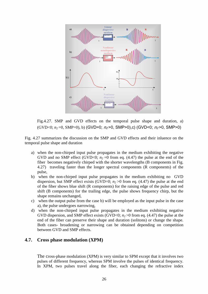
Fig.4.27. SMP and GVD effects on the temporal pulse shape and duration, a)

(GVD<0; n2 =0, SMP=0), b) (GVD=0; n2 >0, SMP>0),c) (GVD<0; n2 >0, SMP>0)

Fig. 4.27 summarizes the discussion on the SMP and GVD effects and their inluence on the

temporal pulse shape and duration

a) when the non-chirped input pulse propagates in the medium exhibiting the negative

GVD and no SMP effect (GVD<0; n2 =0 from eq. (4.47) the pulse at the end of the

fiber becomes negatively chirped with the shorter wavelengths (B components in Fig.

4.27) traveling faster than the longer spectral components (R components) of the

pulse,

b) when the non-chirped input pulse propagates in the medium exhibiting no GVD

dispersion, but SMP effect exists (GVD=0; n2 >0 from eq. (4.47) the pulse at the end

of the fiber shows blue shift (R components) for the raising edge of the pulse and red

shift (B components) for the trailing edge, the pulse shows frequency chirp, but the

shape remains unchanged,

c) when the output pulse from the case b) will be employed as the input pulse in the case

a), the pulse undergoes narrowing,

d) when the non-chirped input pulse propagates in the medium exhibiting negative

GVD dispersion, and SMP effect exists (GVD<0; n2 >0 from eq. (4.47) the pulse at the

end of the fiber can preserve their shape and duration (solitons) or change the shape.

Both cases- broadening or narrowing can be obtained depending on competition

between GVD and SMP effects.

4.7. Cross phase modulation (XPM)

The cross-phase modulation (XPM) is very similar to SPM except that it involves two

pulses of different frequency, whereas SPM involve the pulses of identical frequency.

In XPM, two pulses travel along the fiber, each changing the refractive index

27

tInL as the optical power increases. If these two pulses happen to overlap, they

will introduce distortion into the other pulses through XPM. In contrast to SPM, the

fiber dispersion has little impact on XPM. Increasing the fiber effective area reduces

XPM and all other fiber nonlinearities.

4.8. Theoretical description of GVD phenomenon and self-phase

modulation SPM [14,15]

4.8.1. Nonlinear Schrodinger equation

Polarization controls matter-radiation interaction, therefore it plays significant role in

description of phenomena occurring in optical waveguides.

Polarization operator for N molecules is described with the equation

m

mPP rrˆ

(4.49)

where Pm(r) polarization of molecule m

1

0

ˆˆ mmmmmmm RruRRrqduP rr

(4.50)

Here, mr̂ is the position operator, qma is the electric charge of particle (electron or

nucleus) belonging to molecule m, Rm is a molecular center of mass (or charge), the u–

integration is a number integration that ensures the correct coefficients of the multipolar

expansion of the polarization operator.

Most commonly we shall invoke the dipole approximation where we keep only the first

electric term in the multipolar expansion. The equation (4.50) is then simplified to the form

m

m

mP Rrr - ˆ (4.51)

where m is the dipole moment operator for the mth

molecule and is given by

mmmm Rrq ˆ . (4.52)

The mRr is the Dirac delta function

mm

m

m

RfdrRrrf

Rr

Rr

)(

0 . mRr

(4.53)

The electric field of the laser t,rE interacts with the matter through the polarization

)(rP . The radiation-matter interaction is given by the semiclassical Hamiltonian

28

rrr dPt,E)t(H int . (4.54)

The radiation-matter interaction described by eq. (4.54) can be simplified if we assume the

dipole approximation (eq. (4.51)). The dipole approximation denotes that a single particle has

a size much smaller than the optical wavelength and the particle may be represented by a

point dipole. When the dipole approximation is made we can focus on the temporal response

of a single particle to the electric laser field and the Hamiltonian Hint from (eq.( 4.54)) can be

written as

VrE ttH ,)(int , (4.55)

with the dipole operator

rrV q (4.56)

where the sum runs over all the electrons and nuclei a with charges qa at positions r .

In the semiclassical description of the interaction the material system is treated quantum

mechanically whereas the transverse radiation field t,rE is considered classical.

In the Schrödinger picture, the semiclassical approximation results in the Maxwell-

Liouville equations:

tPtc

tEtc

tE ,4

,1

,2

2

22

2

2rr

r (4.57)

)(ˆ, tPTrtP rr (4.58)

)t(,Hi

t

)t(T

(4.59)

The dynamics of the system is calculated by solving coupled equation for the electric field

and the polarization. As we said, the optical polarization tP ,r is the primary goal of any

theory of optical spectroscopy because it plays a key role for interpreting optical

measurements. To calculate the polarization tP ,r which is a physical observable we have to

average over the statistical ensamble (eq. (4.58)) with the nonequilibrium density operator

)(t by taking a trace Tr. The density operator )(t can be obtained by solving the Liouville

equation (4.59) where HT is given by

intHHHT (4.60)

and describes the Hamiltonian H of the molecular system (matter) and the Hamiltonian of

interaction matter-radiation Hint given by eq. (4.54).

Unfortunately, the equation (4.59) is easy to solve only for the thermal equilibrium

(t=t0) when the electric field of the laser does not disturb the system (Hint=0) and the canonical

density operator is given by

HexpTr

Hexpt0

(4.61)

where 1

BTk

, k is the Boltzman constant, and T is the temperature.

For nonequilibrium situation, when the laser beam begins to interact with the molecular

system, the eq. (4.59) is not easy to solve. Usually, a perturbative order by order expansion of

the response in the fields is applied which indicates that the time-dependent density operator

can be expanded in powers of the electric fields

29

)()()()()( )3()2()1()0( ttttt (4.62)

where (n) denotes th n

th order contribution in the electric field, (0)

(t) = (-).

Upon the substitution (4.62) into (4.58) we obtained the Taylor expansion of the polarizaion

in powers of the radiation field tE ,r

tPtPtPtP ,,,, )3()2()1(rrrr (4.63)

As we explained in chapter 5 this expansion corresponds to the linear and nonlinear optical

processes. The linear term P(1)

is responsible for linear optics, P(2)

is responsible for second-

order processes such as SHG or frequency sum generation, P(3)

is the third-order polarization

that is responsible for THG and many other processes that is measured by a broard variety of

laser techniques such as four-wave mixing, pump-probe spectroscopy or polarization-gating.

It can be shown 9.6

that the nth

order polarizability tP ,)n(r is expressed by the n

th-order

nonlinear response functions S(n)

that provide the complete information about the time

evolution of the system measured by the optical spectroscopy of the nth

order and is given by 9.6

:

0

111,,,)n(

1

0

1

0

)n( ,,,,11

ttttEtttEttESdtdtdttP nnnnntttnn nn rrrr

(4.64)

where the response function S(n)

is given by

,0,,

,,,

1111

2111

)n(

VtVttVttV

ttti

tttS

nn

n

n

nn (4.65)

Here )( is the Heavyside step function [ 1)( for t>0 and 0)( for t<0],

0 represents the equilibrium density operator, which does not evolve with time

only when the molecular Hamiltonia H does not interact with electric field of the laser. The

operator V(t) from eq. (4.65) can be expressed as

H

iVH

iV

expexp)( (4.66)

and represents the dipole operator from eq. (4.56) in the interaction picture. One can see from

eqs. (4.64-4.66) that the polarization response P(n)

is expressed by the n-time points

correlation functions.

For the linear response P(1)

that controls all linear spectroscopy optical measurements

(for example absorption, spontaneous Raman scattering) the response function S(1)

is

simplified to the from

)0(,111

)1( VtVti

tS

(4.67)

and represents well known two-points correlation functions. These functions describe

dynamics of vibrational relaxation in IR and Raman spectroscopy through the vibrational

correlation function )0()( QtQ and dynamics of reorientational relaxation. The higher-order

response functions are a little more complicated, but at some approximations they can be

30

factorized and expressed as a product of two-time point correlation functions. The exact form

of various responses for a specific nonlinear spectroscopy, including pump-probe,

polarization-getting, echoes, coherent Raman the reader can find in Mukamel’s book [14].

The equation (4.57) simplifies to the following wave equation

2

2

02

2

02

2

2

2 1

t

)t(P

t

)t(P

t

)t(E

c)t(E NLL

r,r,r,r, (4.68)

where )t(PL r, and )t(PNL r, are linear and non-linear polarization, accordingly, so )t(PL r,

is the first term in the (4.4) expression and )t(PNL r, includes all remaining terms.

Let us assume that electromagnetic wave is quasi-monochromatic, so its spectral width is

much smaller than frequency of the centre of wave packet 0 ( 10 / ). This

approximation is met for pulses of duration ps.100 , since the frequency of centre is of

the order of s15

0 10 .

It is convenient to separate the fast varying part 0 and slowly varying with time the pulse

envelope (slowly varying envelope approximation) and put down a wave as

.c.ctiexpt,Ext,E 02

1rr

(4.69)

and

.c.ctiexpt,Pxt, LL 02

1rrP

(4.70)

.c.ctiexpt,Pxt, NLNL 02

1rrP

(4.71)

where x

is the unit polarization vector in x direction. Expressing polarization through the

electric susceptibilities of the appropriate order in time domain /)(

xx tt 1 and

321

3 tt,tt,tt)(

xxx we obtain

///

xxL dt)t,(ttt, rErP

1

0 (4.72.a)

321321321

3

0 dtdtdt)t,()t,()t,(tt,tt,ttt, xxxNL rErErErP

(4.72.b)

and using (4.69) we get

////

xxL dtttiexp)t,(Ettt,P

0

1

0 rr

dtiexp,E

~~xx 00

10

2

r (4.73)

where )(

xx~ 1 and 0 ,E

~r denote the susceptibility and the electric field in the frequency

domain after the Fourier transformation. We express t,PNL r in the similar way. Generally,

the response functions 321

3 tt,tt,tt)(

xxx are complex function of time. The nonlinear

response of the system can be simplified significantly if we assume that the response is

immediate. It is the drastic simplification because it is only electron polarization that is

31

immediate, vibrational degrees of freedom related to oscillations of molecule nuclei are much

slower and the corresponding response of nuclei is not immediate after application of pulse of

electric field. Obviously, this approximation can not be applied for description of the

stimulated Raman scattering, because these are vibrations which decide about the Raman

phenomenon. However, in first approximation, when we discuss the influence of pulses of

time duration ps.100 and we are not concerned of Raman effects, we can use that

approximation. Then, the response function can be written

)tt()tt()tt(tt,tt,tt )(

xxx

)(

xxx 321

3

321

3 (4.74)

where )tt( 1 function is the Dirac delta function (4.53)

The equation (4.72.b) takes the form of

t,t,t,t,NL rErErErP 3

0 (4.75)

and if we use (4.71) we obtain

t,Et,P NLNL rr 0 (4.76)

where NL denotes nonlinear contribution to dielectric constant

23

4

3t,ExxxxNL r (4.77)

After substitution (4.69) - (4.71) to (4.68) we obtain the Helmholz equation

02

0

2 E~

kE~

(4.78)

where:

ck

0 ; NLxx

~ 11 (4.79)

and

dttiexpt,E,E~

00

rr (4.80)

To derive the Helmholtz equation for the nonlinear regime, additional assumption of NL

=const was needed, which is not generally valid due to the dependence on the field intensity.

Let us assume that in the first approximation that due to slowly varying envelope

approximation the approximation NL =const employed in solving (4.68) is acceptable. Like

in the linear approximation, the real and the imaginary part of dielectric constant depend on

refraction coefficient n~ and absorption coefficient ~

2

02 )k/~in~( (4.81)

In the nonlinear regime the refraction coefficient n~ and the absorption coefficient depend on

field intensity and usually they take the form 2

2 Ennn~ , 2

2 E~ (4.82)

where

3

28

3xxxxRe

nn , 30

24

3xxxxIm

nc

(4.83)

32

Applying the method of variables separation, which we have already used in chapter 1 in

order to solve the Helmholtz equation for the linear case, we can write the intensity of the

field 0 ,rE~

as a product of the field component y,xF in perpendicular plane to the

propagation of wave, the component of slowly varying envelope in the z direction

0 ,zA~

and the fast varying component of ziexp 0

ziexp,zA~

y,xF,rE~

000 (4.84)

where 0 is the wave vector (we called it the propagation constant in chapter 1) and is the

first term in Taylor series expansion

... 3

3

02

2

01006

1

2

1 (4.85)

where

0

m

m

md

d ...,m 21 (4.86)

Substituting (4.84 ) into Helmholtz equation (4.78) we obtain

022

02

2

2

2

F

~k

y

F

x

F (4.86 )

02 2

0

2

0

A~~

z

A~

i (4.87)

We can determine the wave vector ~

from the equation (4.86) analogously to the method

shown in chapter 1, where we described the propagation of modes in optical waveguides.

Using (4.81), we can approximate the dielectric constant by

nnnnn 222 (4.88)

where n is a nonlinear term of the refraction index and it is expressed by the equation

0

2

22k

iEnn

(4.89)

The equation (4.86) can be solved using the first-order perturbation theory. Namely, if 2n , the equation (4.86) is a solution of F(x,y) for the mode distribution of HE11 in a

single-mode optical waveguide that was described in chapter 1. Having solution of the zero-

order, F(x,y), we insert the perturbation of nn2 to the equation (4.86) and solve it using the

first-order perturbation method

(4.90)

where

(4.91)

dxdyy,xF

dxdyy,xFnk

2

2

0

33

One can calculate E(r,t) from the equation (4.69) and polarizations of )t(PL r, and )t(PNL r,

from (4.72a) via substitution

c.ctziexpt,zAy,xFxt, 002

1

rE (4.92)

where A(z,t) is the inverse Fourier transform of ),z(A~

0

dtizAtzA 00 exp,~

2

1,

. (4.93)

),z(A~

0 can be derived from the equation (4.87) that can be written as

A~iz

A~

0

(4.94)

where 2

0

2 ~

is substituted by )~

( 002 .

In order to transform t,zA to the time domain, the inverse Fourier transform should be

applied, (4.93), for both sides of (4.94) that leads to

Ait

Ai

t

A

z

A

2

2

21

2 (4.95)

Using (4.89) in (4.91) we can calculate and insert it to (4.95). Finally, we get time-

domain wave equation

AAiAt

Ai

t

A

z

A 2

2

2

21

22

(4.96)

This equation is known as the nonlinear Schrödinger equation (NLS) and plays a significant

role in description of GVD effects and nonlinearity of optical waveguides.

that includes the following effects:

- losses in optical waveguide – term A2

,

- group velocity of the centre of pulse - t

A

1 ,

- dispersion of the group velocity GVD - 2

2

2

2 t

Ai

,

- nonlinearity of optical waveguide AAi2

where

effcA

n 02 (4.97)

and

dxdyy,xF

dxdyy,xF

Aeff

4

2

2

(4.98)

Typical values of the parameters in equation (4.96) in standard glass single-mode optical

waveguides for 1.5 m :

34

W/m.n 220

2 1062 ; 210020 mAeff ;

km/W 1101 ; km/ps2

2 20

4.8.2. Inclusion of the higher order nonlinear effects in the nonlinear

Schrödinger equation

Despite its usefulness for description of light propagation in optical waveguides for

pulses longer than 1ps, the Schrödinger equation (4.96) is insufficient for characterisation of

nonlinear phenomena such as the stimulated Raman scattering (SRS), the stimulated Brillouin

scattering (SBS), the self-phase modulation (SPM), the four-wave mixing. Furthermore, the

inclusion of the third term, 3 , in Taylor expansion (4.85) is occasionally necessary.

Now, we will show the methods that include these effects. Generally, the response

functions 321

3 tt,tt,tt)(

xxx are complex function of time. As we have shown in the

previous chapter, the nonlinear response of a system can significantly be simplified if the

immediate response is assumed

)tt()tt()tt(tt,tt,tt )(

xxx

)(

xxx 321

3

321

3 (4.99)

This is the drastic simplification since only electron polarisation is immediate, vibrations of

molecule nuclei are much slower and the corresponding response to the applied electric field

is not immediate This approximation definitely cannot be used for description of the

stimulated Raman scattering, since these are vibrations that decide on the Raman scattering.

The phenomenon can be included by the response function R [16]

321

3

321

3 ttttttRtt,tt,tt (4.100)

where 1ttR is a nonlinear response function, normalized so that

dt)t(R =1. The

expression (4.100) is only correct for non-resonance conditions.

Substituting (4.100) to (4.72b) we get

1

2

11

3

0 dtt,rEttRt,rEt,rPt

NL

(4.101)

Applying analogous procedure as we employed in chapter 3, one can show [17] that in the

frequency domain the equation similar to the Helmholtz one can be derived

ddz,E~

z,E~

z,E~

R~

cikE

~knE

~1212112

23

0

2

0

22

(4.102)

where 1 R~

is the Fourier transform of the response function of 1ttR . Treating the

right-hand expression as a perturbation, we can derive the expression for the mode

distribution, F(x,y), and for the wave vector

~

(4.103)

35

where is a perturbation, but it is not expressed by formula (4.91). Defining slowly

varying function A(z,t) in the same way as in the equation (4.92) we get [17]

tdtt,zAtRt,zAt

ii

t

A

t

Ai

t

AA

z

A '2

0

3

3

3

2

2

21 1

622

(4.104)

The equation (4.104) is valid not only for the slowly varying envelope approximation used

before, but also for the pulses as short as several optical cycles.

The response function, tR , can be written as follows

thftftR RRR 1 (4.105)

where the first term describes immediate polarisation from electronic contribution, and the

second term, Rf , depicts contribution of polarisation coming from vibrations. The function of

thR is connected with the Raman amplification described in chapter 4.3.

RRR h~

Imfcn

g 3

0

0 (4.106)

where Im corresponds to the imaginary part of the Fourier transform Rh~

of the response

function of thR . The real term can be derived from the imaginary one using Kramers-

Kronig relation [18]. Applying various models for vibrations one can derive the analytical

form of the thR . Below, the form of thR for dumped oscillations is presented [19]

12

2

21

2

2

2

1

tsin

texpthR (4.107)

The equation 4.104 can be simplified if we assume that pulses are short ( ps50 ), however

noticeably longer than the time interval of just few optical cycles ( fs100 ). Then

expansion into Taylor series can be applied

222

t,zAt

tt,zAtt,zA ''

(4.108)

Defining the first moment of the response function as

0

d

h~

ImdfdttthfdtttRT R

RRRR (4.109)

and taking into account the fact that

dt)t(R =1 we get the equation after inserting (4.108)

into (4.109)

T

AATAA

T

iAAi

T

A

T

AiA

z

AR

2

2

0

2

3

3

3

2

2

2

622

(4.110)

36

This equation is expressed in the reference system that moves with the group velocity, g ,

of the centre of the wave packet where

ztz

tTg

1

(4.111)

When comparing the equation 4.110 with the nonlinear Schrödinger equation (NLS) (4.96),

we can notice three new terms, which are responsible for

3

3

3

6 T

A

- introduces the third order dispersion. The inclusion of this dispersion

turned out to be necessary for short pulses since they represent a very broad spectrum,

AAT

i 2

0

- introduces the first derivative of nonlinear polarization and it is

responsible for self-steeping and shock formation [ 20 ]

T

AATR

2

is connected with Raman effect. It is responsible for the self-frequency

shift [21] and it is induced by intrapulse scattering.

In practice, when a pulse duration ps50 , the last two terms are negligible. Moreover,

the first term is also insignificant if the wavelength of the pulse centre is not close to the

wavelength, where the dispersion coefficient D=0. Therefore, we can write

022

2

2

2

2

AA

T

AA

i

z

Ai

(4.112)

This equation is similar to the nonlinear Schrödinger equation (4.96), if the moving

reference system is applied, (4.111).

When the peak-power of pulses reaches the order of 1GW/cm2, fifth-order nonlinear

terms should be included in (4.4). This effect can be included through replacement of

parameter in (4.112) by the modified parameter

2

02

0 11

AbAb

As

s

(4.113)

where sb denotes the saturation parameter. In practice, for glass optical waveguides

2Abs <<1 and equation 4.112 can successfully be used even in case of relatively high

peak-powers. However if saturation effect exists, we take it into account through inclusion

(4.113) into the equation (4.112). Such equation is named the cubic-quintic NLS equation.

4.8.3. The derivation of formula for pulse broadening due to the GVD effect

[15]

In chapter 3 we showed that the group velocity dispersion, GVD, causes pulse

broadening. In that chapter, we will derive the formulas that were used in chapter 3.

The analysis will be confined to pulses longer than ps50 , so the nonlinear

Schrödinger equation (4.112) can be applied

37

AAT

AA

i

z

Ai

2

2

2

2

22

(4.114)

As we said in chapter 4.8.2, this equation includes

loses in an optical waveguide – term A2

,

group velocity – it was the term t

A

1 in eq. (4.96) that was taken into account in

(4.114) via introduction the moving reference system

ztz

tTg

1

group velocity dispersion, GVD, 2

2

2

2 T

A

,

nonlinearity of optical waveguide, AA2

Let us introduce normalized the time scale with respect to the input pulse duration 0

00

g

zt

T

(4.115)

and the normalized pulse amplitude, ,zU , that is independent of loses in an optical

waveguide

,zU/zexpP,zA 20 (4.116)

where 0P denotes power of the input pulse.

Using relations of (4.115-4.116) in 4.114 we get

UU

L

zexpU

L

sgn

z

Ui

NLD

2

2

2

2

2

(4.117)

where 12 sgn represemts the sign of 2 parameter that characterises GVD, and

2

2

0

DL ,

0

1

PLNL

. (4.118)

DL and NLL is known in literature as the dispersion length and the nonlinear length,

respectively and characterize the optical length L of a fiber, for which dispersion effects and

nonlinear effects are negligible (4.117)

if the length of optical waveguide fulfils the condition of DLL and NLLL ,

both the group velocity dispersion effects, GVD, and the nonlinear effects can be

neglected,

if NLLL but DLL , the nonlinear effects are negligible, but GVD is important

resulting in temporal pulse broadening,

if DLL but NLLL , the dispersion effects are negligible in comparison to the

nonlinear effects, time pulse distortion is caused by the self-phase modulation, SPM.

38

Of course the first case, when both GVD and SMP effects are negligible, is the most

desirable case for optical transmission. We can estimate DL and NLL from eq. (4.118) for

certain input powers 0P and duration of pulses 0 , assuming typical values of

km/ps2

2 20 and 113 kmW in the window of 1550nm. For short pulses and low

input powers 0P , i.e. WP 10 , ps10 , the second case with GVD dominates with

12

2

00

P

L

L

NL

D (4.119)

For longer pulses and high input powers 0P , e.g. WP 10 , the self-phase modulation SMP

dominates

12

2

00

P

L

L

NL

D . (4.120)

Summarizing this part of discussion we can say that

for standard telecommunications optical waveguides of the length of 50-80km in the

window of 1550nm km/ps2

2 20 and pulses of 0 >100ps, kmLD 500 , the

dispersion effects, GVD, are negligible ( DLL ). However for shorter pulses of 0 of

the order of 1 ps, mLD 50 , the dispersion effect is not negligible since DLL .

Let us consider now the influence of GVD dispersion on the pulse broadening. In

chapter 3 we showed that the group velocity dispersion, GVD, causes pulse broadening

(3.27a). Now we will derive that expression and other formulas, which are useful in analysis

of pulse distortion caused by GVD dispersion. Let us neglect the influence of nonlinearity,

SPM, inserting =0 into (4.114) and (4.117) we obtain

2

2

2

2 T

U

z

Ui

(4.121)

The equation can simply be solved in the frequency domain, if we use the inverse Fourier

transform

dTiexp,zU~

T,zU

2

1 (4.122)

Using (4.122) in (4.121) we get the equation

U~

z

U~

i 2

22

1

(4.123)

with the solution

z

iexp,U

~,zU

~ 2

22

0 (4.124)

39

The expression (4.124) illustrates that the dispersion effect, GVD, causes phase shift of each

frequency separately. The magnitude of that shift depends on the optical path z of a pulse

propagating in an optical fiber. Coming back to the time domain (4.122) and substituting

(4.124) we obtain

dTizi

exp,U~

T,zU

2

22

02

1 (4.125)

where ,U~

0 is the normalized amplitude of the input pulse for z=0 in the frequency

domain and is expressed via the Fourier transform

dTTiexpT,U,U~

00 (4.126)

Let us assume the incident pulse has the Gaussian shape

2

0

2

20

TexpT,U (4.127)

where 0 the is pulse duration defined as the half-width for the intensity corresponding to 1/e

of its maximal value and is related to the full width at half maximum through the relation of

002

1

665122 .lnTFWHM (4.128)

Using (4.127) in (4.126) and (4.125) we get

zi

Texp

zi

T,zU2

2

0

2

2

1

2

2

0

0

2

(4.129)

Comparing (4.127) with (4.129) we can state that the pulse keeps the Gaussian shape but it

exhibits broadening

2

1

2

0 1

DL

zz (4.130)

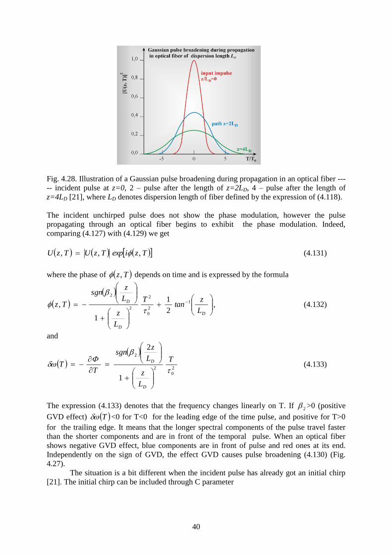
40

Fig. 4.28. Illustration of a Gaussian pulse broadening during propagation in an optical fiber ---

-- incident pulse at z=0, 2 – pulse after the length of z=2LD, 4 – pulse after the length of

z=4LD [21], where LD denotes dispersion length of fiber defined by the expression of (4.118).

The incident unchirped pulse does not show the phase modulation, however the pulse

propagating through an optical fiber begins to exhibit the phase modulation. Indeed,

comparing (4.127) with (4.129) we get

T,ziexpT,zUT,zU (4.131)

where the phase of T,z depends on time and is expressed by the formula

D

D

D

L

ztan

T

L

z

L

zsgn

T,z 1

2

0

2

2

2

2

1

1

, (4.132)

and

2

0

2

2

1

2

T

L

z

L

zsgn

TT

D

D

(4.133)

The expression (4.133) denotes that the frequency changes linearly on T. If 2 >0 (positive

GVD effect) T <0 for T<0 for the leading edge of the time pulse, and positive for T>0

for the trailing edge. It means that the longer spectral components of the pulse travel faster

than the shorter components and are in front of the temporal pulse. When an optical fiber

shows negative GVD effect, blue components are in front of pulse and red ones at its end.

Independently on the sign of GVD, the effect GVD causes pulse broadening (4.130) (Fig.

4.27).

The situation is a bit different when the incident pulse has already got an initial chirp

[21]. The initial chirp can be included through C parameter

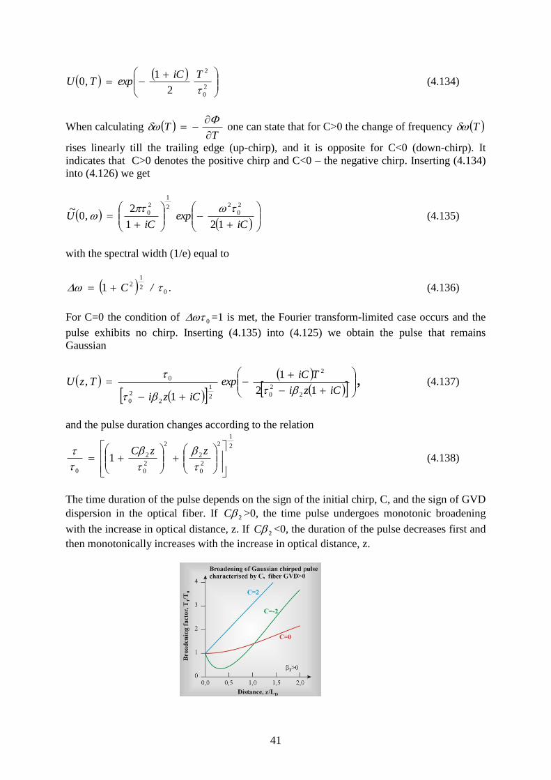
41

2

0

2

2

10

TiCexpT,U (4.134)

When calculating T

T

one can state that for C>0 the change of frequency T

rises linearly till the trailing edge (up-chirp), and it is opposite for C<0 (down-chirp). It

indicates that C>0 denotes the positive chirp and C<0 – the negative chirp. Inserting (4.134)

into (4.126) we get

iCexp

iC,U

~

121

20

2

0

22

1

2

0 (4.135)

with the spectral width (1/e) equal to

02

121 /C . (4.136)

For C=0 the condition of 0 =1 is met, the Fourier transform-limited case occurs and the

pulse exhibits no chirp. Inserting (4.135) into (4.125) we obtain the pulse that remains

Gaussian

iCzi

TiCexp

iCzi

T,zU12

1

1 2

2

0

2

2

1

2

2

0

0

, (4.137)

and the pulse duration changes according to the relation

2

1

2

2

0

2

2

2

0

2

0

1

zzC (4.138)

The time duration of the pulse depends on the sign of the initial chirp, C, and the sign of GVD

dispersion in the optical fiber. If 2C >0, the time pulse undergoes monotonic broadening

with the increase in optical distance, z. If 2C <0, the duration of the pulse decreases first and

then monotonically increases with the increase in optical distance, z.

42

Fig. 4.29. Broadening of Gaussian chirped pulse characterised by C parameter during

propagation in optical waveguide of positive dispersion, GVD>0, ----- pulse for C=0, C=2 –

pulse with input positive GVD dispersion, C=-2 pulse with input negative GVD dispersion

[21]. When a fibre shows GVD<0 the same curves characterize bandwidth broadening when

we change signs of C.

It is easy to understand the initial effect of pulse shortening looking at (4.138) equation. If

2C <0 at the input, a pulse shows its own negative GVD (characterized by C parameter)

opposite to GVD of the fiber in which it starts to propagate. It means that shorter

wavelengths, which travelled faster at the input, start to demonstrate a delay effect and longer

wavelengths starts to travel faster down the fiber. It leads to compensation of the GVD

dispersion effect. The pulse reaches minimum for such the distance of minz in optical

waveguide when both effects are compensated (GVD = 0). The distance can be derived form

the (4.138) expression

DLC

Cz

2min1

(4.139)

For minz the pulse is the shortest min and it shows transform-limited spectral band width,

,

212

0

1 /min)C(

(4.140)

where 1min .

When the pulse propagates further, for distances longer than minz GVD effect of the optical

waveguide starts to dominate and the pulse becomes exhibit broadening again.

Now, we will return to the analysis of the self-phase modulation (SPM). As we said in

chapter 3 this effect comes from the fact that the nonlinear refraction coefficient )(n 2

depends on pulse intensity )t(I

)t(I)(n)(n)(n 20 . (4.141)

Let us assume that GVD is negligible. In eq. (4.117) we can put 02 to obtain

UUL

ie

z

U

NL

z2

(4.142)

where U is the normalized amplitud defined by (4.116), NLL is the nonlinear length

1

0

PLNL (4.143)

where depends on the nonlinear refraction index 2n (4.141), oP is the peak power of the

puls. Equation (4.142) can be easily solved substituting NLiexpVU where NL is

nonlinear phase (4.47b). We get

0

z

V , 2V

L

e

z NL

zNL

(4.150)

43

The solution of eq.(4.142) is constant, the integral over the length L is

T,LiexpT,UT,LU NL0 (4.151)

where U(0,T) is the normalized amplitude for z=0, the nonlinear phase NL for z=L is

obtained as

NLeffNL L/LT,UT,L2

0 (4.152)

where the effective length effL is defined as

/LexpLeff 1 (4.153)

Maximum of nonlinear phase is in the center of the temporal pulse (T=0), because we showed

that NL depends on the intensity. Thus, for the amplitude normalized as U(0,0)=1, we get

eff

NL

eff

max LPL

L0 (4.154)

As we showed in chapter 4.6 the spectral broadening of the pulse due to SMP comes from

the time dependence of nonlinear phase NL . The transient frequency 0 T along

the pulse can be calculated from

2,0 TU

TL

L

TT

NL

effNL

(4.155)

The temporal broadening depends on the shape of U(0.T). Let us assume that the shape is

given by

m

z

TiCexpT,U

2

02

10 (4.156)

Substituting (4.156) into (4.155) we get

mT

Texp

T

T

L

L

T

mT

m

NL

eff2

2

0

12

00

(4.157)

From (4.157) one can see that for T<0 (leading edge of the pulse), 0 (red shift), for

T=0 (puls center), 0 , for T>0 (trailing edge), 0 (blue shift).

Derived here formulas help to understand the phase modulation (frequency chirp) shown in

Fig. 4.21 which illustrates the principle of automodulation SPM.

44

1. R.H. Stolen, E.P. Ippen, Raman gain in glass optical waveguides, Appl. Phys. Lett.

Vol.22, no.6, 1973

2. 3.V. V. Raman and K. S. Krishnan, "A new type of secondary radiation", Nature 121,

501-2 (1928)

3. J. Hecht, Raman amplifiers boost system margins at high speed, Laser Focus World

37(6) (June, 2001) 135-140

4. J. Hecht, Mitigating nonlinear effects is essential to long-haul transmission systems,

Laser Focus World 38(5) (May, 2002) 155-162

5. M. Islam, M. Nietubyc, Not a pretty picture, WDM solutions 3(3) (March 2001)

6. Halina Abramczyk, Introduction to Laser Spectroscopy, Elsevier, New York, 2005

7. M. N. Islam, IEEE Journal of selected Topics in Quantum Electronics, vol.8, no. 3,

2002

8. Y. R. Shen, The principles of Nonlinear Optics, Wiley, New York, 1984, chap. 10

9. R. G. Smith, Appl. Opt. 11, 2489 (1972)]

10. G. P. Agrawal, Nonlinear fiber optics, 3rd

edition, Academic Press, 2001, p. 361

11. R. H. Stolen, C. Lin, Phys. Rev. A 17, 1448 (1978)]

12. G. P. Agrawal, Nonlinear fiber optics, 3rd

edition, Academic Press, 2001, p. 104

13. G. P. Agrawal, Nonlinear fiber optics, 3rd

edition, Academic Press, 2001, p.105

14. S. Mukamel, Principles of Nonlinear Spectroscopy, Oxford, 1995

15. G. P. Agrawal, Nonlinear fiber optics, 3rd

edition, Academic Press, 2001

16. K.J. Blow, D. Wood, IEEE J. Quantum Electron. 25, 2665 (1989)]

17. P.M. Mamyshev, S. V. Chernikov, Opt. Lett. 15, 1076 (1990)]

18. M.Schubert, B. Wilhelmi, Nonlinear Optics and Quantum Electronics, Wiley, New

York, 1986

19. K.J. Blow, D. Wood, IEEE J. Quantum Electron. 25, 2665 (1989)]

20. S. Blair, K. Wagner, Opt. Quantum Electron. 30, 697 (1998)

21. G. P. Agrawal, "Nonlinear fiber optics", 3rd

edition, Academic Press, 2001