Nonlinear Parameter Estimation

Q550: Models in Cognitive Science

Lecture 8

•  We want to estimate the optimum parameters for our cognitive model using an objective function. Then we can quantitatively compare our models.

Some Issues in Parameter Estimation: 1.  Linear vs. nonlinear models 2.  Data considerations/Fitting approaches

Techniques for Parameter Estimation

Linear vs. Nonlinear Models •  Estimating parameters in a cognitive model is similar to

estimating regression coefficients

•  However, regression models belong to the general linear class, whereas cognitive models are usually nonlinear…this affects our search for parameters

•  Linear models satisfy a special condition: the average of the predictions from two different sets of parameters = the prediction produced by the average of the two sets of parameters. Nonlinear models do not satisfy this property

Linear vs. Nonlinear Models •  Estimating the parameters of a linear model can usually

be done with a single-step algorithm that is guaranteed to produce an optimal solution

•  There are no single-step solutions for estimating the parameters of a nonlinear model: we must search the (often complex) parameter space for the optimal solution

•  There is no guarantee that the optimal solution will be found (but we can still try)

Data Considerations •  Before estimating parameters, we need to be clear

about the data to be used.

•  Assume that we have 10 participants per group, 11 delay conditions, and 200 observations per delay point

1.  Aggregate modeling

2.  Individual modeling

3.  Hierarchical modeling

1. Aggregate Modeling •  Easiest approach: one set of parameters estimated for

normal group; another set for the amnesic group

•  However, this assumes no individual differences within group…e.g., all individuals in the normal condition have the same decay rates

•  Importance of individual differences (see Estes; Ashby & Maddox, etc.)

•  A bad example from early learning theory: incremental strength learning models vs. all-or-none models. What if AON was generating model w/ individual differences on amount of training required to find solution to problem

•  Cf. Exponential law of practice (Brown, Heathcote, & Mewhort, 2000, PBR)

The Danger of Averaging Over Subjects •  Pooling or averaging data from many subjects can

produce misleading results as an artifact of grouping (Sidman, 1960)

•  Averaging can produce results that do not characterize any subject who participated. More importantly, it can produce a result supporting theory X when perhaps it shouldn’t (Estes)

•  E.g.: Manis (1971) tested children in a discrimination learning task…stimuli were simple objects, and your will have to learn which feature is the diagnotic one (shape, color, position, etc.)

Trial 1:

Trial 2:

Trial 3:

Trial 4:

Trial 5:

Trial 6:

+

+

+

+

+

+

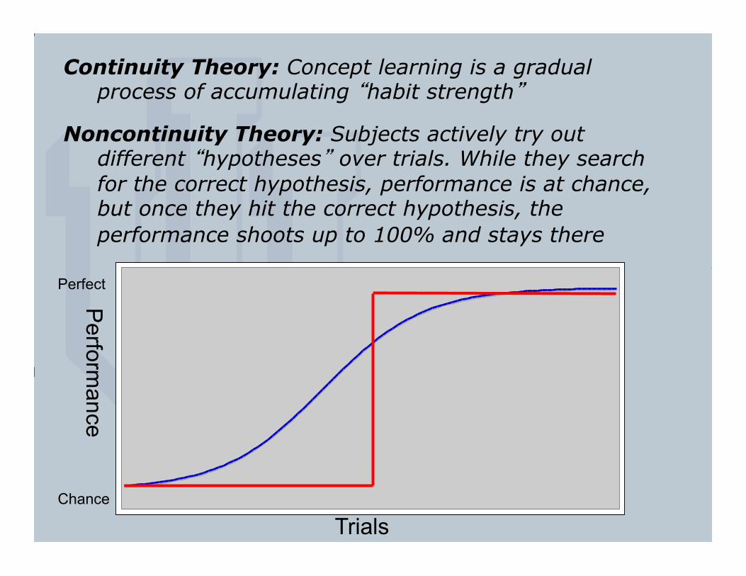
Continuity Theory: Concept learning is a gradual process of accumulating “habit strength”

Noncontinuity Theory: Subjects actively try out different “hypotheses” over trials. While they search for the correct hypothesis, performance is at chance, but once they hit the correct hypothesis, the performance shoots up to 100% and stays there

Trials

Perform

ance

Chance

Perfect

Here are the averaged data. Continuity is right!!

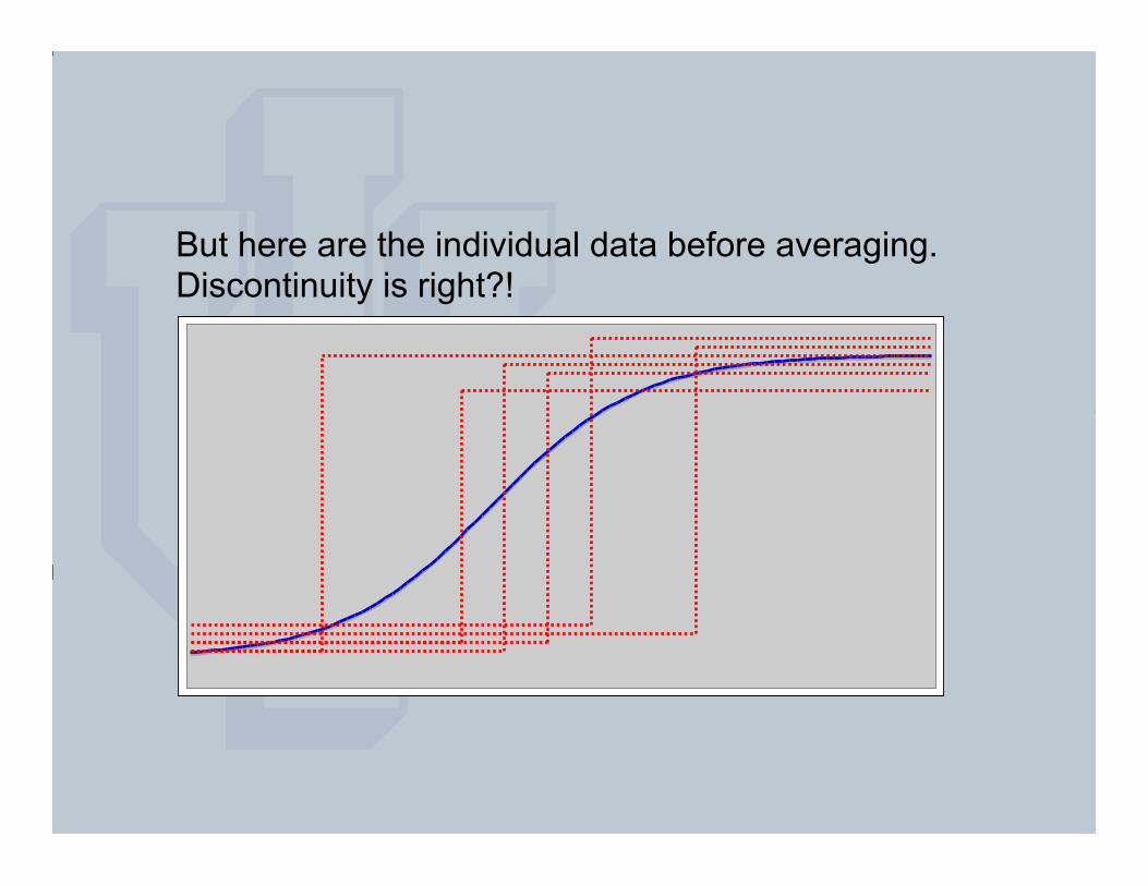
But here are the individual data before averaging. Discontinuity is right?!

2. Individual Modeling •  Estimate parameters for each individual separately

•  Separate parameters (and even separate models) may be best fit for different individuals

•  Requires a large amount of data from each subject

•  Preferred method if parameters represent cognitive factors you expect to vary across subjects

•  Compute the parameters for each group, then compare the parameter distributions across groups for significant differences…does the mean decay rate differ?

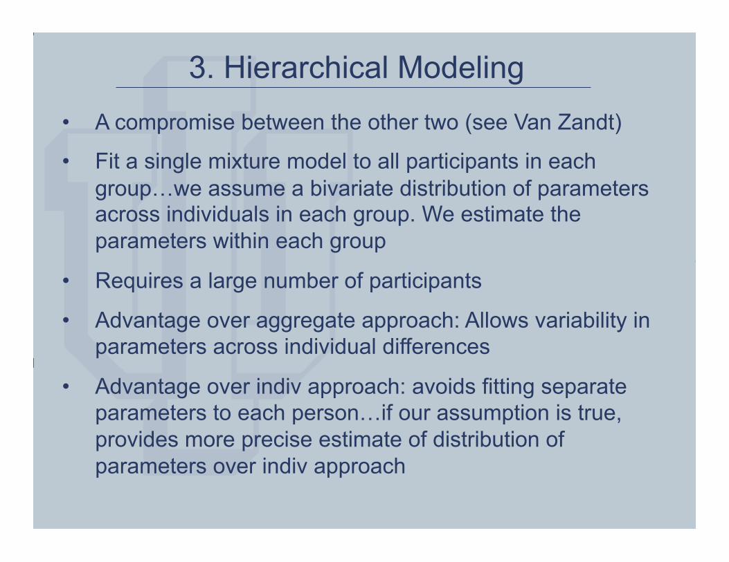
3. Hierarchical Modeling •  A compromise between the other two (see Van Zandt)

•  Fit a single mixture model to all participants in each group…we assume a bivariate distribution of parameters across individuals in each group. We estimate the parameters within each group

•  Requires a large number of participants

•  Advantage over aggregate approach: Allows variability in parameters across individual differences

•  Advantage over indiv approach: avoids fitting separate parameters to each person…if our assumption is true, provides more precise estimate of distribution of parameters over indiv approach

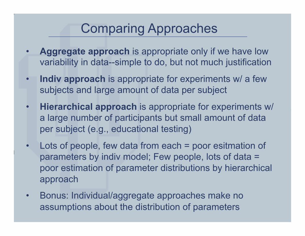
Comparing Approaches •  Aggregate approach is appropriate only if we have low

variability in data--simple to do, but not much justification

•  Indiv approach is appropriate for experiments w/ a few subjects and large amount of data per subject

•  Hierarchical approach is appropriate for experiments w/ a large number of participants but small amount of data per subject (e.g., educational testing)

•  Lots of people, few data from each = poor esitmation of parameters by indiv model; Few people, lots of data = poor estimation of parameter distributions by hierarchical approach

•  Bonus: Individual/aggregate approaches make no assumptions about the distribution of parameters

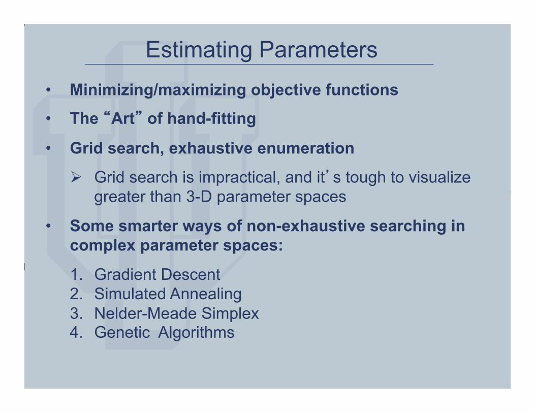
Estimating Parameters •  Minimizing/maximizing objective functions

•  The “Art” of hand-fitting

•  Grid search, exhaustive enumeration

Ø  Grid search is impractical, and it’s tough to visualize greater than 3-D parameter spaces

•  Some smarter ways of non-exhaustive searching in complex parameter spaces:

1.  Gradient Descent 2.  Simulated Annealing 3.  Nelder-Meade Simplex 4.  Genetic Algorithms

Gradient Descent Algorithms •  Take steps downhill to determine parameter values that

minimize the objective function

LOOP •  Determine starting point--take a step to all possible

adjacent grid points, and compute change in SSE

•  Determine which point produces the steepest descent, and take a step in that direction

•  We now have a new set of parameter values that are better starting values

UNTIL (Flat)

•  Continue process until we reach a point where a move in any direction leads uphill…this is the set of parameters that minimizes the objective function

Amnesics

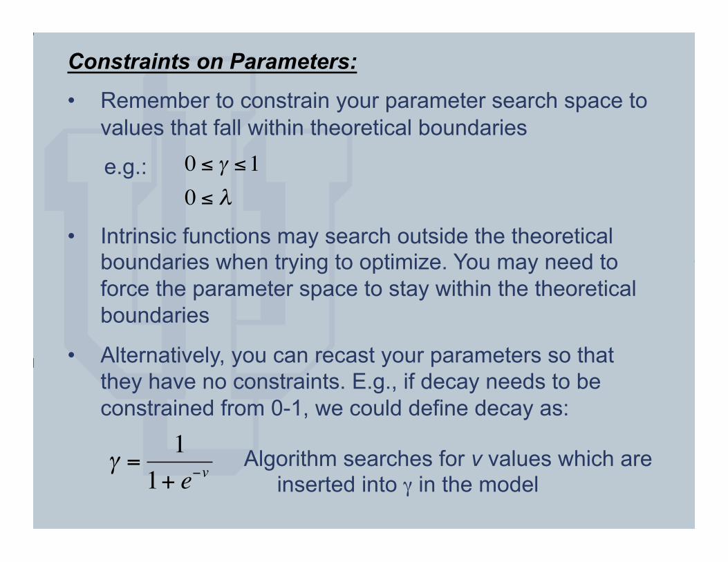
Constraints on Parameters:

•  Remember to constrain your parameter search space to values that fall within theoretical boundaries

e.g.:

•  Intrinsic functions may search outside the theoretical

boundaries when trying to optimize. You may need to force the parameter space to stay within the theoretical boundaries

•  Alternatively, you can recast your parameters so that they have no constraints. E.g., if decay needs to be constrained from 0-1, we could define decay as:

€

0 ≤ γ ≤1

0 ≤ λ

€

γ =1

1+ e−v

Algorithm searches for v values which are inserted into γ in the model

Flat Minimum Problem:

•  If the parameter space is has a flat region, the search process may terminate prematurely b/c changed in the objective function are too small to detect improvements

•  Near the minimum point, changes in one parameter can be compensated for by changes in another

•  Flatness near the minimum produces parameter estimates with large standard errors

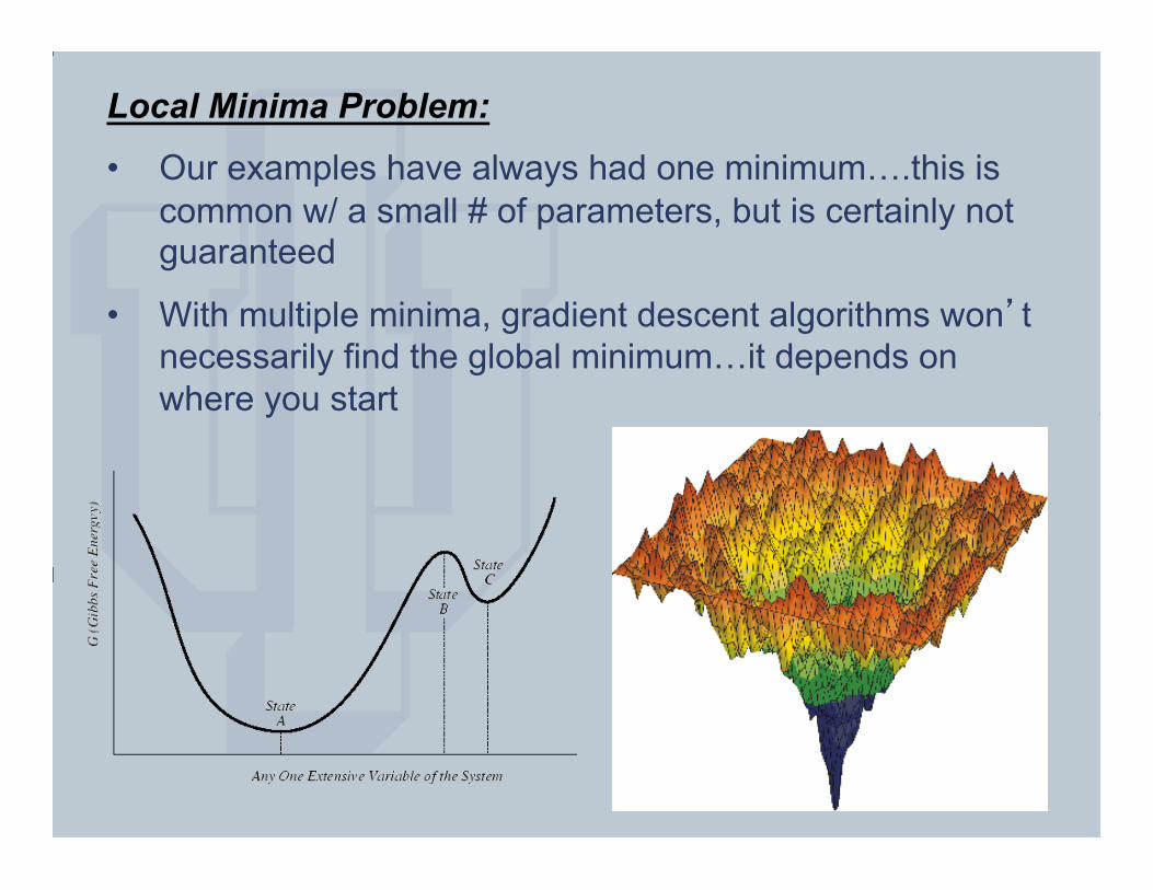
Local Minima Problem:

•  Our examples have always had one minimum….this is common w/ a small # of parameters, but is certainly not guaranteed

•  With multiple minima, gradient descent algorithms won’t necessarily find the global minimum…it depends on where you start

Local Minima Problem:

•  One way to avoid getting stuck in a local minimum is to try several starting positions

•  As the # of parameters increases, the possibility of more local minima increases

Simulated Annealing

•  Useful in highly nonlinear spaces with large # of parms

•  Based on annealing in metallurgy: heating/cooling of a material to increase the size of its crystals and reduce their defects

•  If you were fitting 100 parameters with a grid search method, you could find the global minimum in several million years of computation Ø  Simulated annealing will quickly find a “pretty good”

solution Ø  Cf. Particle swarm algorithm

Simulated Annealing •  Select a starting position

LOOP •  Randomly select a new position and evaluate it

compared to old position •  With probability p, select superior; w/ probability (1-p)

select inferior •  Increment p UNTIL (Flat)

Early in search, bounces up and down a lot to escape local minima; later in search, converges toward global minimum

Nelder-Meade Simplex •  Gradient descent requires smooth parameter spaces to

compute gradient--otherwise, use a non-derivative based search

•  Simplex: minimize the area of a tetrahedron in n-dimensional space (aka: tripod search)

Tetrahedron (3-simplex)

Petachoron (4-simplex)

Hexa-5-tope (5-simplex)

…etc.

Nelder-Meade Simplex •  Select 3 random points for the simplex

LOOP •  Select a 4th point within the simplex, or at an edge •  For each point, compute the objective function, and

retain the best 3 of 4 points (step towards optimum solution)

UNTIL (no further improvement)

Many optimal simplex algorithms exist…plenty of code online. It is one of the most popular parameter estimation algorithms b/c of its efficiency and reliability

In Matlab: fminsearch() or fminunc()

Downhill

Amnesics

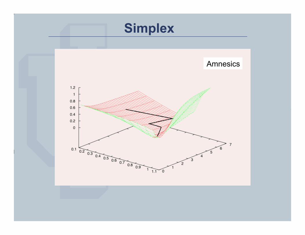
Simplex

Amnesics

Downhill

Simplex

Running a Simplex in Matlab [Parms, Obj_Func] = fminsearch(‘Model’, Parms, options)

•  Parms is a vector that has one element for each parameter

•  Model is the name of a file that returns an objective function (Model.m should be in same directory)

•  You have to give fminsearch starting values for the parameters, and it will start intelligently walking in the space from this starting point to the lowest point of Obj_Func

•  So, 2 files: Model.m and Fit_Model.m in same directory

Using fminsearch() Model.m: Makes predictions using parameters handed to it and

returns the value of objective function (min)

function [resp] = Model(Parms)% a vector w/ 1 value for each parameter

global Data •  Make model predictions in Pred vector

•  Compute obj_func (e.g., SSE) between Data and Pred

resp = obj_func

end % function Model

Using fminsearch() Fit_Model.m: The simplex controlling selection of parameters to hand

to the model each iteration (step of a leg)

global Data;

Parms = zeros(1,k); % k = # of parameters we need to fit

Data = [#, #, #, ….]; % Data you are trying to fit model to

Parms(1) = #; Parms(2) = #; % Initial parameters; just a guess

Options = optimset(‘Display’, ‘Iter’);

[Parms, obj_func] = fminsearch(‘Model’, Parms, options); •  Print optimum parameters and final minimized objective function

Optimum parameters for retention model? Homework (Due Feb 17): What are the optimum parameters for our

retention model if we assume that it is the correct model for Amnesiacs and Normals? Hand in code, optimum parameters, minimized SSE

Data(:,1) = [0.95 0.91 0.92 0.90 0.86 0.91 0.80 0.82 0.81 0.74 0.73]; % Normals Data(:,2) = [0.96 0.91 0.91 0.81 0.76 0.75 0.72 0.65 0.64 0.61 0.60]; % Amnesiacs Use fminsearch() to find the optimum parameters for each group

Our parameters are λ (sensitivity parameter) and γ (decay rate)

…but let’s simplify this model

€

p A | x(t)[ ] =eλoAγ

t

eλoAγ

t

+ eλoBγt

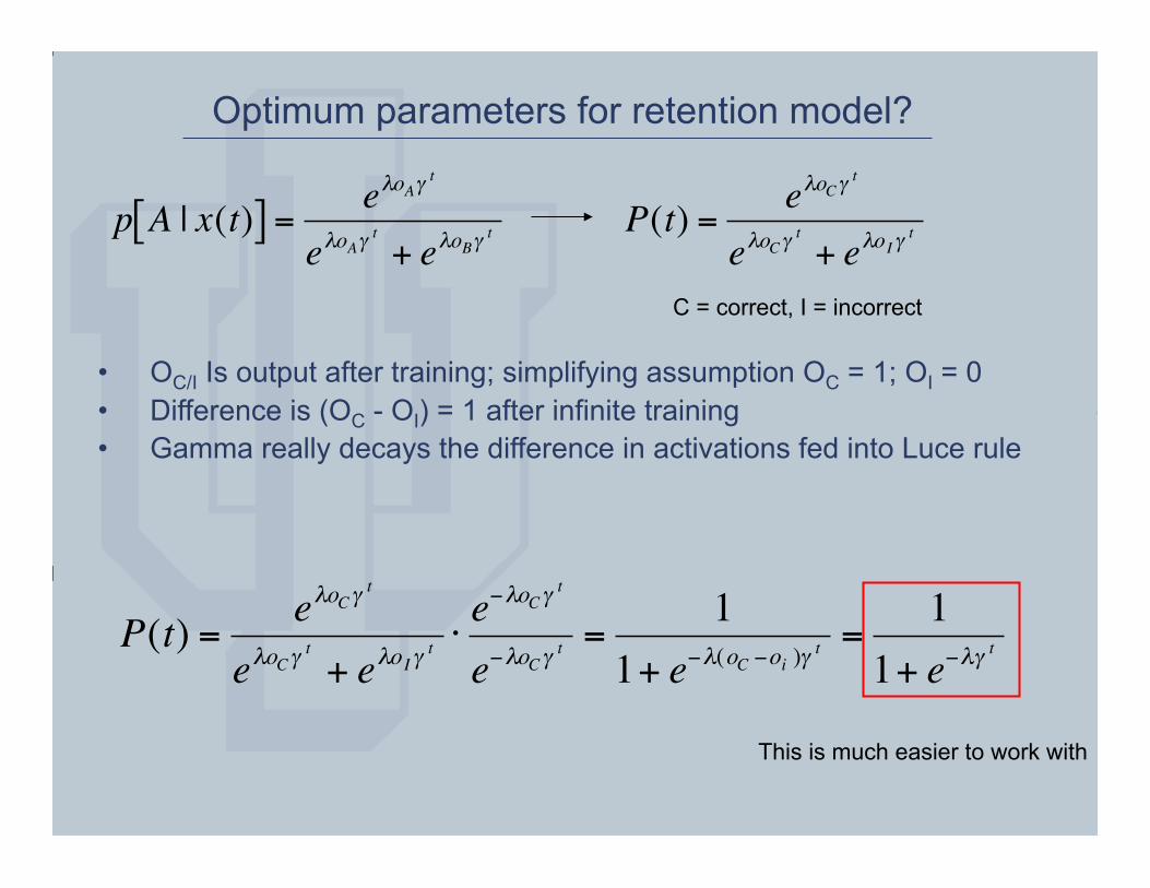
Optimum parameters for retention model?

•  OC/I Is output after training; simplifying assumption OC = 1; OI = 0 •  Difference is (OC - OI) = 1 after infinite training •  Gamma really decays the difference in activations fed into Luce rule

€

p A | x(t)[ ] =eλoAγ

t

eλoAγ

t

+ eλoBγt

€

P(t) =eλo

Cγ t

eλo

Cγ t

+ eλo

Iγ t

C = correct, I = incorrect

€

P(t) =eλo

Cγ t

eλo

Cγ t

+ eλo

Iγ t⋅e−λo

Cγ t

e−λo

Cγ t

=1

1+ e−λ(o

C−o

i)γ t

=1

1+ e−λγ t

This is much easier to work with

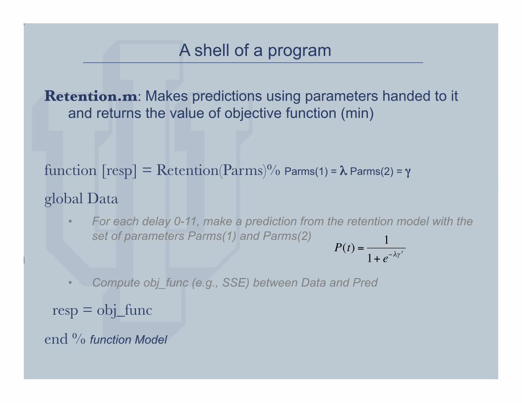
A shell of a program Retention.m: Makes predictions using parameters handed to it

and returns the value of objective function (min)

function [resp] = Retention(Parms)% Parms(1) = λ Parms(2) = γ

global Data •  For each delay 0-11, make a prediction from the retention model with the

set of parameters Parms(1) and Parms(2)

•  Compute obj_func (e.g., SSE) between Data and Pred

resp = obj_func

end % function Model

€

P(t) =1

1+ e−λγ t

A shell of a program Fit_Retention.m: The simplex controlling selection of parameters to

hand to the model each iteration (step of a leg)

global Data;

Parms = zeros(1,2); % k = 2 of parameters we need to fit (lambda, gamma)

Group = zeros(11,2); % Data: 11 observations for 2 groups Group(:,1) = [0.95 0.91 0.92 0.90 0.86 0.91 0.80 0.82 0.81 0.74 0.73]; % Normals

Group(:,2) = [0.96 0.91 0.91 0.81 0.76 0.75 0.72 0.65 0.64 0.61 0.60]; % Amnesiacs

Data = Group(:,1) % let’s fit normals first

Parms(1) = 1; Parms(2) = 0.8; % Initial parameters; just a guess

Options = optimset(‘Display’, ‘Iter’);

[Parms, obj_func] = fminsearch(‘Retention’, Parms, options);