NONLINEAR MIXED EFFECTSMODELS

An Overview and Update

Marie DavidianDepartment of Statistics

North Carolina State University

http://www.stat.ncsu.edu/∼davidian

Based on: Davidian, M. and Giltinan, D.M. (2003), “Nonlinear Models

for Repeated Measurement Data: An Overview and Update,”

JABES 8, 387–419

IBC2004 1

Outline

• Introduction

• The Setting

• The Model

• Inferential Objectives and Model Interpretation

• Implementation

• Extensions and Recent Developments

• Discussion

IBC2004 2

Introduction

Common situation in agricultural, environmental, and biomedical

applications:

• A continuous response evolves over time (or other condition) within

individuals from a population of interest

• Inference focuses on features or mechanisms that underlie individual

profiles of repeated measurements of the response and how these vary

in the population

• A theoretical or empirical model for individual profiles with parameters

that may be interpreted as representing such features or mechanisms is

available

IBC2004 3

Introduction

Nonlinear mixed effects model: aka hierarchical nonlinear model

• A formal statistical framework for this situation

• A “hot ” methodological research area in the early 1990s

• Now widely accepted as a suitable approach to inference, with

applications routinely reported and commercial software available

• Many recent extensions, innovations

IBC2004 4

Introduction

Nonlinear mixed effects model: aka hierarchical nonlinear model

• A formal statistical framework for this situation

• A “hot ” methodological research area in the early 1990s

• Now widely accepted as a suitable approach to inference, with

applications routinely reported and commercial software available

• Many recent extensions, innovations

Objective of this talk: An updated review of the model and survey of

recent advances

IBC2004 4

The Setting

Example 1: Pharmacokinetics

• Broad goal : Understand intra-subject processes of drug absorption,

distribution, and elimination governing achieved concentrations

• . . . and how these vary across subjects

• Critical for developing dosing strategies and guidelines

IBC2004 5

The Setting

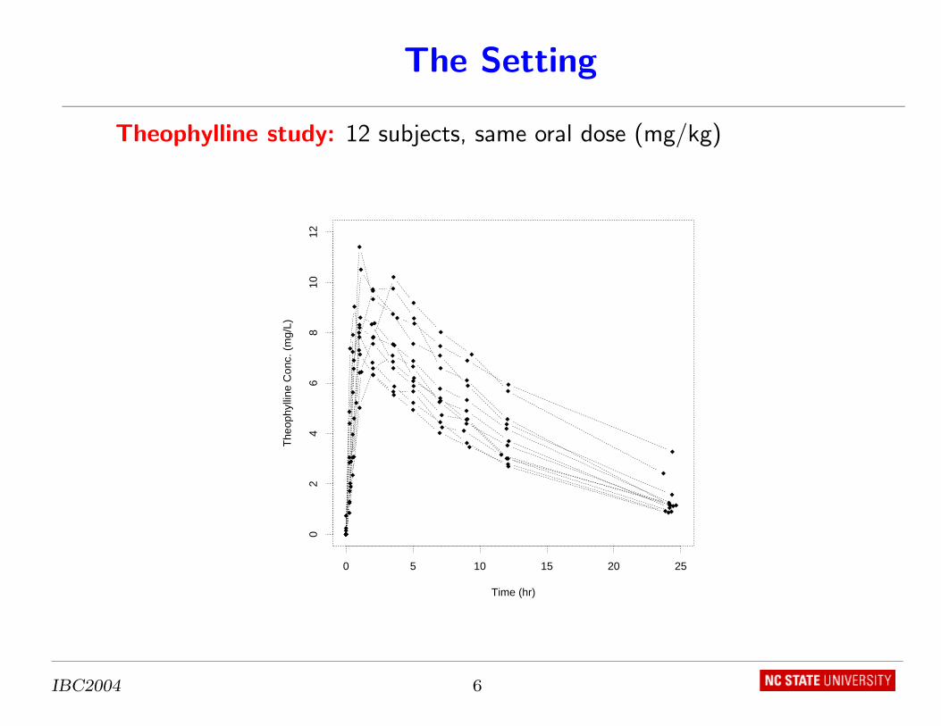
Theophylline study: 12 subjects, same oral dose (mg/kg)

Time (hr)

The

ophy

lline

Con

c. (

mg/

L)

0 5 10 15 20 25

02

46

810

12

IBC2004 6

The Setting

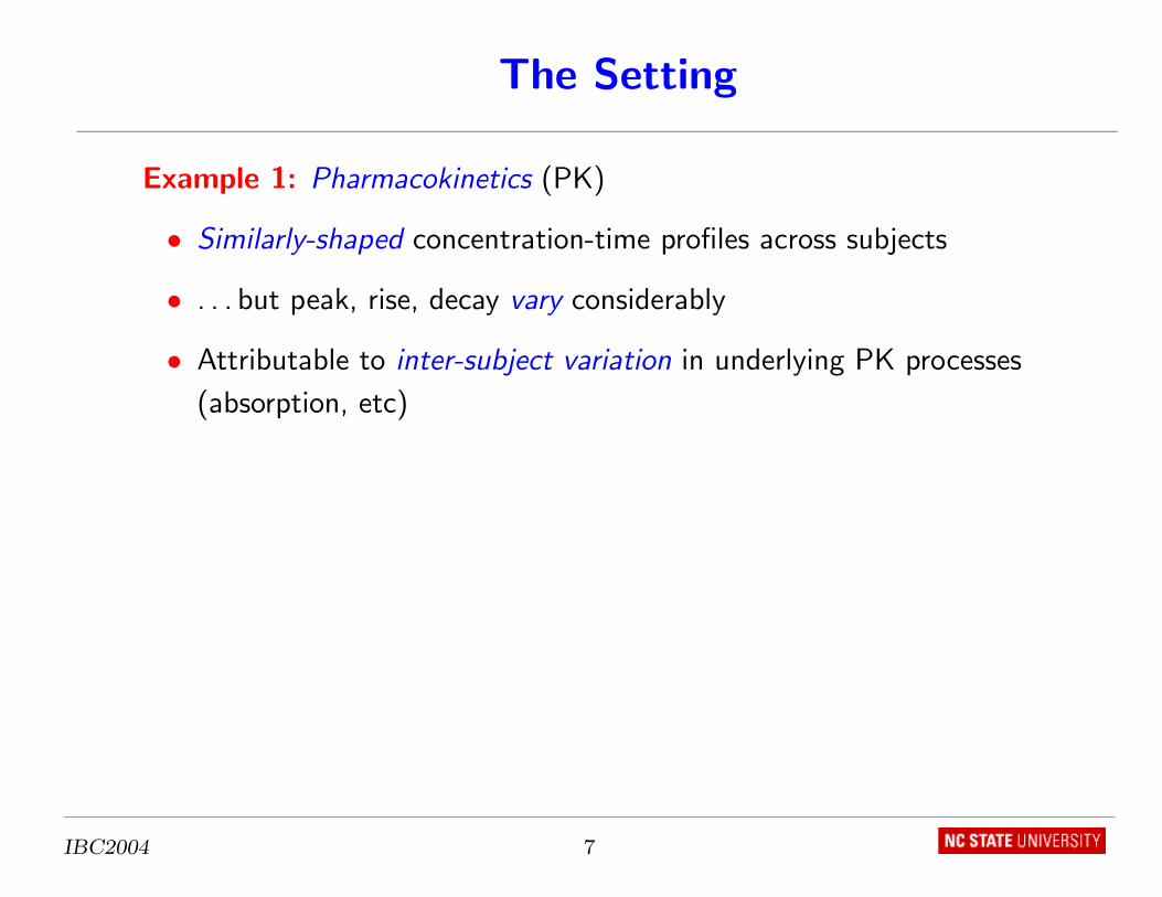
Example 1: Pharmacokinetics (PK)

• Similarly-shaped concentration-time profiles across subjects

• . . . but peak, rise, decay vary considerably

• Attributable to inter-subject variation in underlying PK processes

(absorption, etc)

IBC2004 7

The Setting

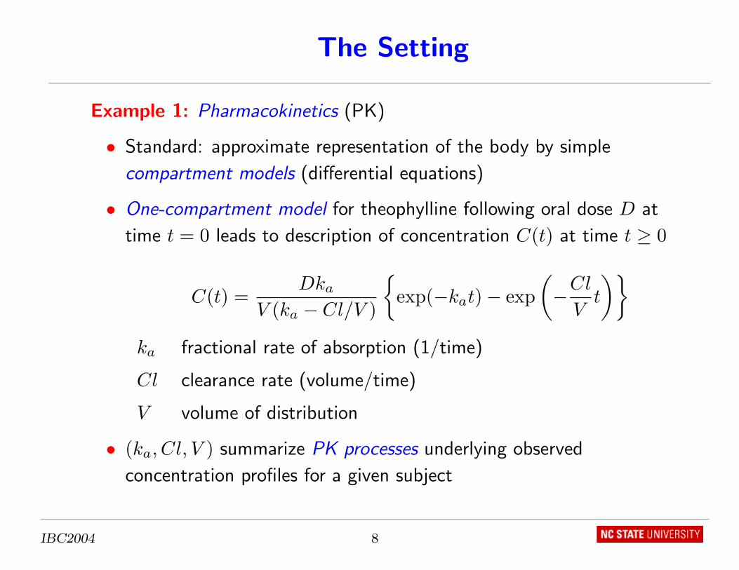
Example 1: Pharmacokinetics (PK)

• Standard: approximate representation of the body by simple

compartment models (differential equations)

• One-compartment model for theophylline following oral dose D at

time t = 0 leads to description of concentration C(t) at time t ≥ 0

C(t) =Dka

V (ka − Cl/V )

{exp(−kat)− exp

(−Cl

Vt

)}

ka fractional rate of absorption (1/time)

Cl clearance rate (volume/time)

V volume of distribution

• (ka, Cl, V ) summarize PK processes underlying observed

concentration profiles for a given subject

IBC2004 8

The Setting

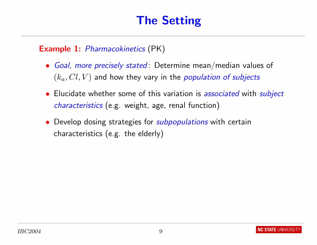
Example 1: Pharmacokinetics (PK)

• Goal, more precisely stated : Determine mean/median values of

(ka, Cl, V ) and how they vary in the population of subjects

• Elucidate whether some of this variation is associated with subject

characteristics (e.g. weight, age, renal function)

• Develop dosing strategies for subpopulations with certain

characteristics (e.g. the elderly)

IBC2004 9

The Setting

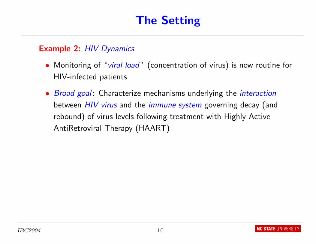
Example 2: HIV Dynamics

• Monitoring of “viral load ” (concentration of virus) is now routine for

HIV-infected patients

• Broad goal : Characterize mechanisms underlying the interaction

between HIV virus and the immune system governing decay (and

rebound) of virus levels following treatment with Highly Active

AntiRetroviral Therapy (HAART)

IBC2004 10

The Setting

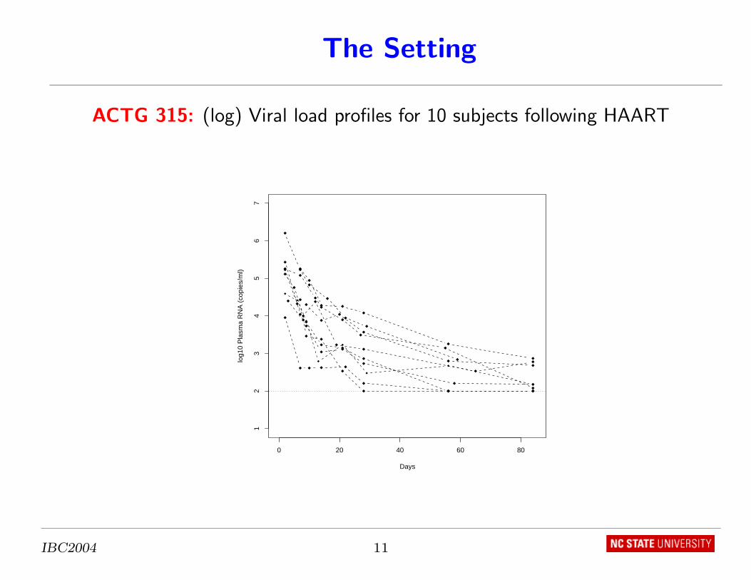
ACTG 315: (log) Viral load profiles for 10 subjects following HAART

0 20 40 60 80

12

34

56

7

Days

log1

0 P

lasm

a R

NA

(co

pies

/ml)

IBC2004 11

The Setting

Example 2: HIV Dynamics

• Similarly-shaped profiles with different decay patterns

• Complication – Viral load assay has lower limit of quantification

IBC2004 12

The Setting

Example 2: HIV Dynamics

• Represent body by system of ordinary differential equations, e.g.

dX

dt= (1− ε)kV T − δX

dV

dt= pX − cV

X, T size of infected, uninfected immune cell populations

V size of viral population, c viral clearance

δ infected cell death rate, p viral production rate

k probability of infection, ε treatment efficacy

• Parameters characterize intra-subject mechanisms related to

interaction between virus and immune system

IBC2004 13

The Setting

Example 2: HIV Dynamics

• Complication – Expression for V (viral load) may not be available in a

closed form

• Further complication – All states of the system of ODEs may not have

been measured

• Goal, more precisely stated : Elucidate “typical ” parameter values

(mean/median), variation across subjects, associations with measures

of pre-treatment disease status

IBC2004 14

The Setting

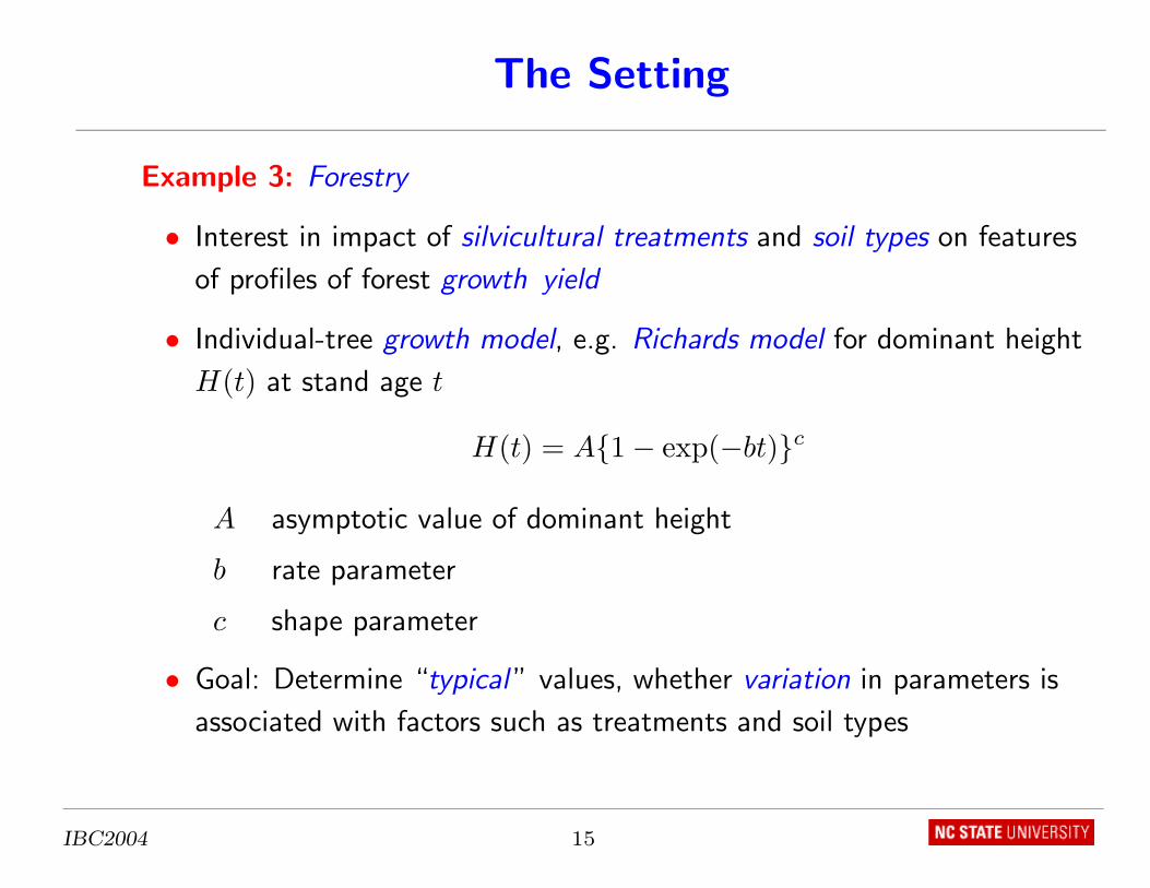
Example 3: Forestry

• Interest in impact of silvicultural treatments and soil types on features

of profiles of forest growth yield

• Individual-tree growth model, e.g. Richards model for dominant height

H(t) at stand age t

H(t) = A{1− exp(−bt)}c

A asymptotic value of dominant height

b rate parameter

c shape parameter

• Goal: Determine “typical ” values, whether variation in parameters is

associated with factors such as treatments and soil types

IBC2004 15

The Setting

Further applications:

• Dairy science

• Wildlife science

• Fisheries science

• Biomedical science

IBC2004 16

The Model

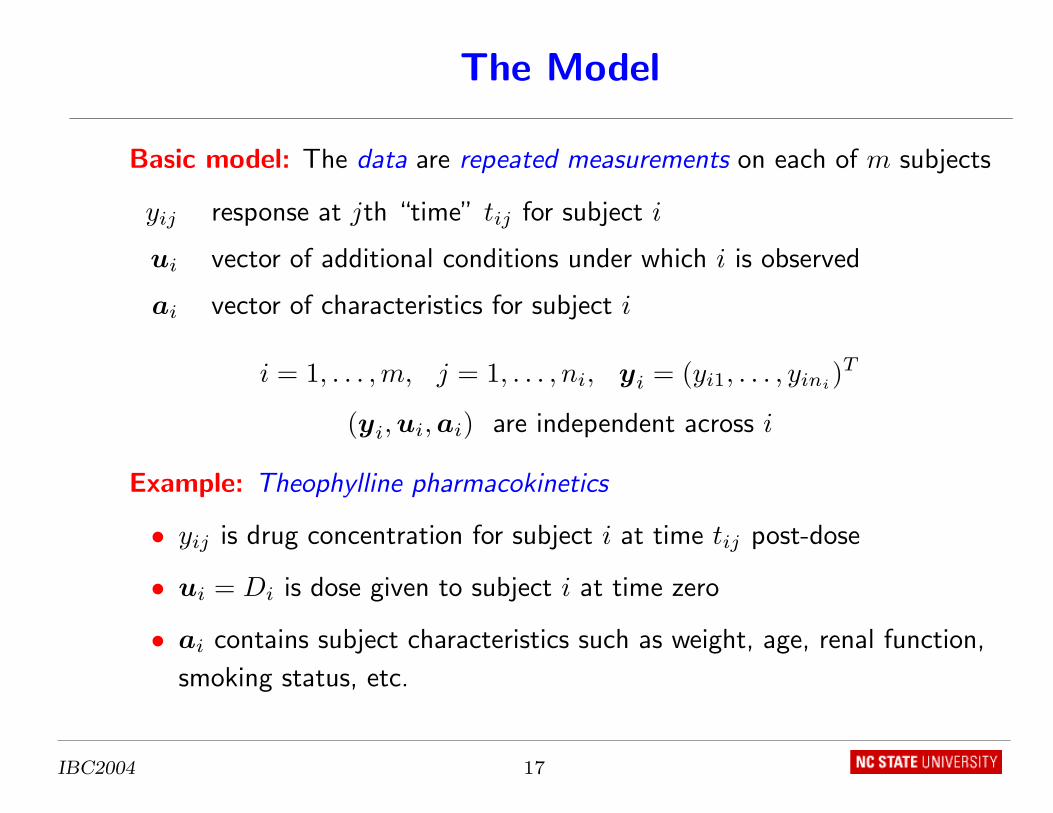
Basic model: The data are repeated measurements on each of m subjects

yij response at jth “time” tij for subject i

ui vector of additional conditions under which i is observed

ai vector of characteristics for subject i

i = 1, . . . , m, j = 1, . . . , ni, yi = (yi1, . . . , yini)T

(yi, ui, ai) are independent across i

Example: Theophylline pharmacokinetics

• yij is drug concentration for subject i at time tij post-dose

• ui = Di is dose given to subject i at time zero

• ai contains subject characteristics such as weight, age, renal function,

smoking status, etc.

IBC2004 17

The Model

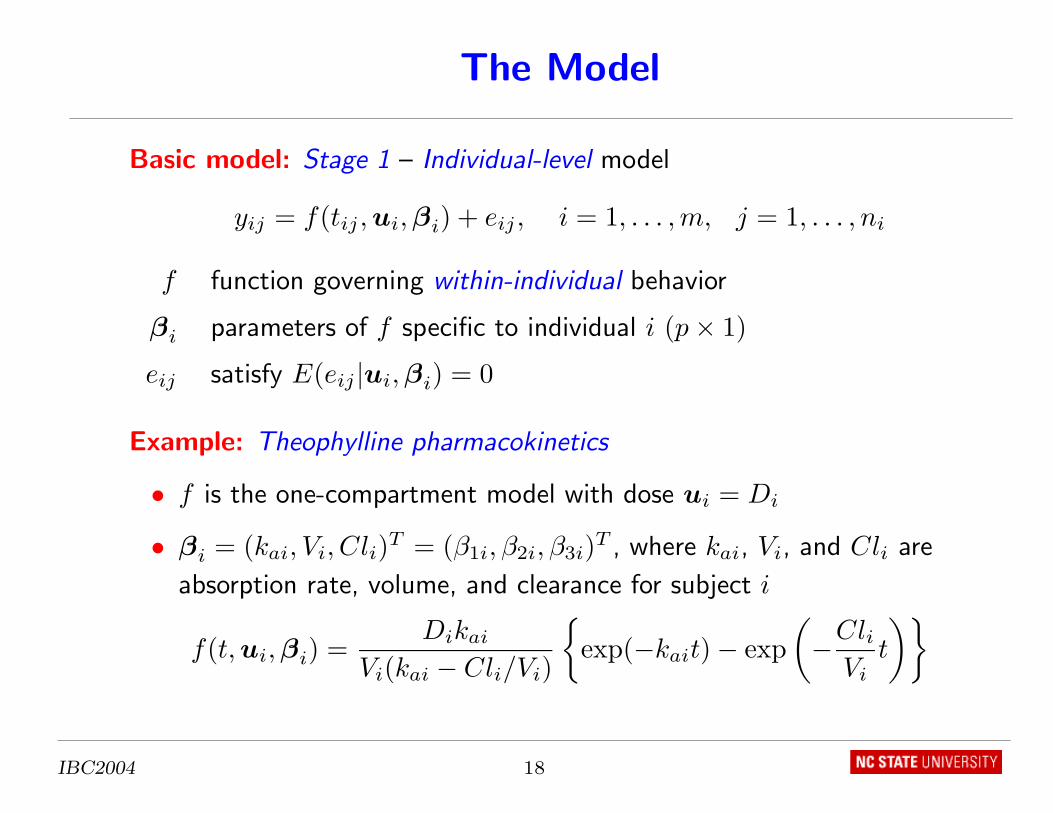
Basic model: Stage 1 – Individual-level model

yij = f(tij , ui, βi) + eij , i = 1, . . . , m, j = 1, . . . , ni

f function governing within-individual behavior

βi parameters of f specific to individual i (p× 1)

eij satisfy E(eij |ui, βi) = 0

Example: Theophylline pharmacokinetics

• f is the one-compartment model with dose ui = Di

• βi = (kai, Vi, Cli)T = (β1i, β2i, β3i)T , where kai, Vi, and Cli are

absorption rate, volume, and clearance for subject i

f(t, ui, βi) =Dikai

Vi(kai − Cli/Vi)

{exp(−kait)− exp

(−Cli

Vit

)}

IBC2004 18

The Model

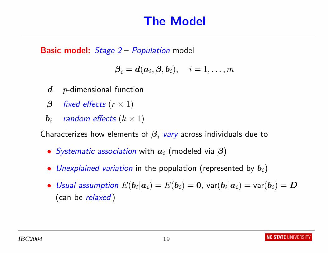
Basic model: Stage 2 – Population model

βi = d(ai, β, bi), i = 1, . . . , m

d p-dimensional function

β fixed effects (r × 1)

bi random effects (k × 1)

Characterizes how elements of βi vary across individuals due to

• Systematic association with ai (modeled via β)

• Unexplained variation in the population (represented by bi)

• Usual assumption E(bi|ai) = E(bi) = 0, var(bi|ai) = var(bi) = D

(can be relaxed )

IBC2004 19

The Model

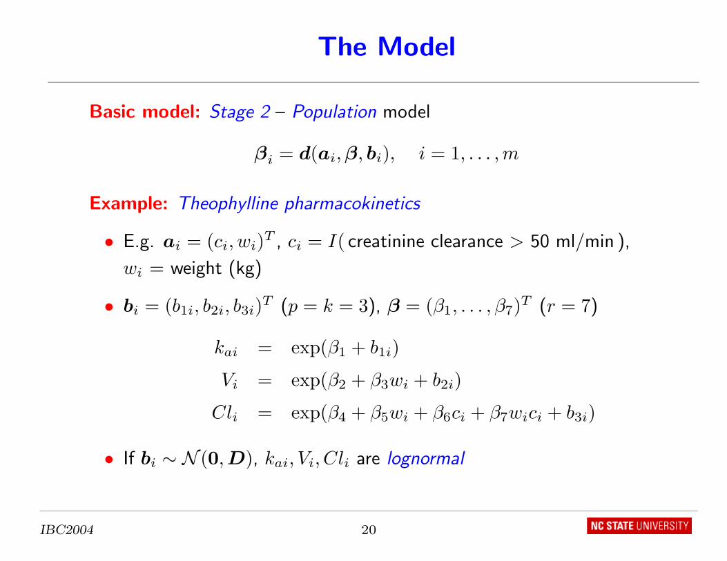
Basic model: Stage 2 – Population model

βi = d(ai, β, bi), i = 1, . . . , m

Example: Theophylline pharmacokinetics

• E.g. ai = (ci, wi)T , ci = I( creatinine clearance > 50 ml/min ),

wi = weight (kg)

• bi = (b1i, b2i, b3i)T (p = k = 3), β = (β1, . . . , β7)T (r = 7)

kai = exp(β1 + b1i)

Vi = exp(β2 + β3wi + b2i)

Cli = exp(β4 + β5wi + β6ci + β7wici + b3i)

• If bi ∼ N (0, D), kai, Vi, Cli are lognormal

IBC2004 20

The Model

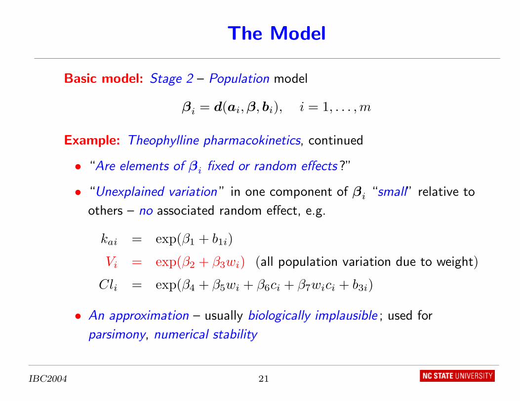
Basic model: Stage 2 – Population model

βi = d(ai, β, bi), i = 1, . . . , m

Example: Theophylline pharmacokinetics, continued

• “Are elements of βi fixed or random effects ?”

• “Unexplained variation ” in one component of βi “small” relative to

others – no associated random effect, e.g.

kai = exp(β1 + b1i)

Vi = exp(β2 + β3wi) (all population variation due to weight)

Cli = exp(β4 + β5wi + β6ci + β7wici + b3i)

• An approximation – usually biologically implausible ; used for

parsimony, numerical stability

IBC2004 21

The Model

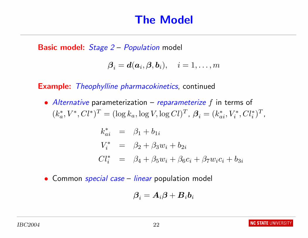
Basic model: Stage 2 – Population model

βi = d(ai, β, bi), i = 1, . . . , m

Example: Theophylline pharmacokinetics, continued

• Alternative parameterization – reparameterize f in terms of

(k∗a, V ∗, Cl∗)T = (log ka, log V, log Cl)T , βi = (k∗ai, V∗i , Cl∗i )T ,

k∗ai = β1 + b1i

V ∗i = β2 + β3wi + b2i

Cl∗i = β4 + β5wi + β6ci + β7wici + b3i

• Common special case – linear population model

βi = Aiβ + Bibi

IBC2004 22

The Model

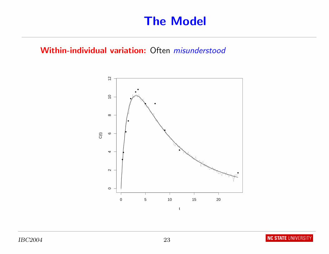
Within-individual variation: Often misunderstood

IBC2004 23

The Model

Within-individual variation: Often misunderstood

t

C(t

)

0 5 10 15 20

02

46

810

12

IBC2004 23

The Model

Within-individual variation: Conceptual perspective

• E(yij |ui, βi) = f(tij , ui, βi) =⇒ f represents i’s “on-average ”

profile (smooth curve)

• f may not capture all within-individual processes perfectly, “local

fluctuations ” =⇒ actual realized profile (jittery line)

• f(t, ui, βi) is average over all possible realizations =⇒ “inherent

tendency ” for i’s profile evolution

• =⇒ βi is “inherent characteristic ” of i

• =⇒ Interest focuses on inherent properties of individuals rather than

actual response realizations

IBC2004 24

The Model

Within-individual variation: Conceptual perspective

• Within-individual stochastic process

yi(t, ui) = f(t, ui, βi) + eR,i(t, ui) + eM,i(t, ui)

E{eR,i(t, ui)|ui, βi} = E{eM,i(t, ui)|ui, βi} = 0

• Thus yij = yi(tij , ui), eR,i(tij , ui) = eR,ij , eM,i(tij , ui) = eM,ij

yij = f(tij , ui, βi) + eR,ij + eM,ij︸ ︷︷ ︸eij

eR,i = (eR,i1, . . . , eR,ini)T , eM,i = (eM,i1, . . . , eM,ini

)T

• eR,i(t, ui) = “realization deviation process ”

• eM,i(t, ui) = “measurement error process ”

IBC2004 25

The Model

Within-individual variation: Conceptual perspective

• Model for eR,i(t, ui) and hence eR,i based on assumptions about

actual realization variance, correlation

var(eR,i|ui, βi) = T1/2i (ui, βi, δ)Γi(ρ)T 1/2

i (ui, βi, δ), (ni × ni)

• Model for eM,i(t, ui) and hence eM,i based on assumptions about

measurement error variance

var(eM,i|ui, βi) = Λi(ui, βi, θ), (ni × ni) diagonal matrix

• Common assumption – realization, measurement error processes

independent =⇒var(yi|ui, βi) = var(eR,i|ui, βi) + var(eM,i|ui, βi) = Ri(ui, βi, ξ)

ξ = (δT , ρT , θT )T

IBC2004 26

The Model

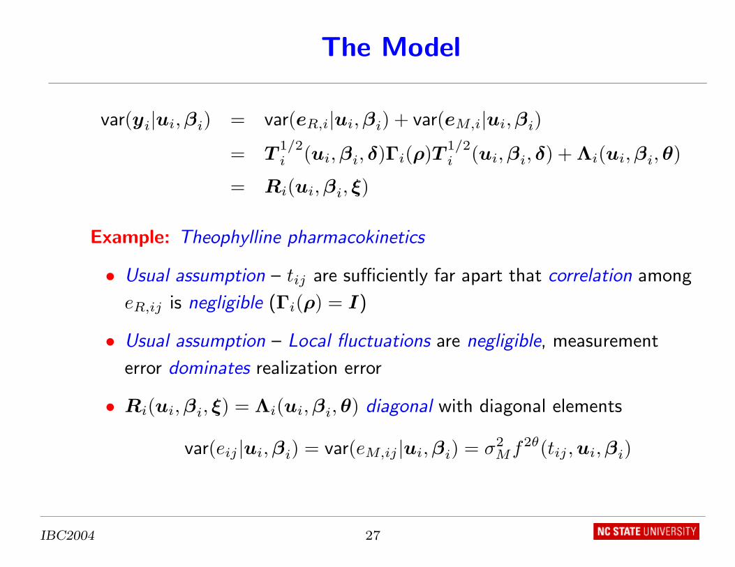
var(yi|ui, βi) = var(eR,i|ui, βi) + var(eM,i|ui, βi)

= T1/2i (ui, βi, δ)Γi(ρ)T 1/2

i (ui, βi, δ) + Λi(ui, βi, θ)

= Ri(ui, βi, ξ)

Example: Theophylline pharmacokinetics

• Usual assumption – tij are sufficiently far apart that correlation among

eR,ij is negligible (Γi(ρ) = I)

• Usual assumption – Local fluctuations are negligible, measurement

error dominates realization error

• Ri(ui, βi, ξ) = Λi(ui, βi, θ) diagonal with diagonal elements

var(eij |ui, βi) = var(eM,ij |ui, βi) = σ2Mf2θ(tij , ui, βi)

IBC2004 27

The Model

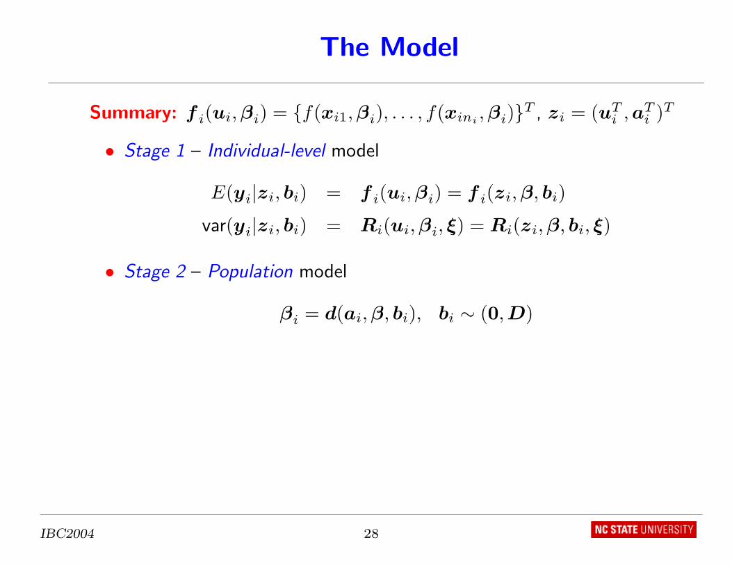
Summary: f i(ui, βi) = {f(xi1, βi), . . . , f(xini, βi)}T , zi = (uT

i , aTi )T

• Stage 1 – Individual-level model

E(yi|zi, bi) = f i(ui, βi) = f i(zi, β, bi)

var(yi|zi, bi) = Ri(ui, βi, ξ) = Ri(zi, β, bi, ξ)

• Stage 2 – Population model

βi = d(ai, β, bi), bi ∼ (0, D)

IBC2004 28

The Model

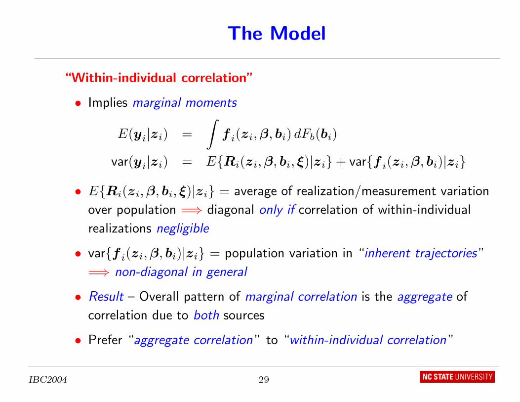
“Within-individual correlation”

• Implies marginal moments

E(yi|zi) =∫

f i(zi, β, bi) dFb(bi)

var(yi|zi) = E{Ri(zi, β, bi, ξ)|zi}+ var{f i(zi, β, bi)|zi}

• E{Ri(zi, β, bi, ξ)|zi} = average of realization/measurement variation

over population =⇒ diagonal only if correlation of within-individual

realizations negligible

• var{f i(zi, β, bi)|zi} = population variation in “inherent trajectories ”

=⇒ non-diagonal in general

• Result – Overall pattern of marginal correlation is the aggregate of

correlation due to both sources

• Prefer “aggregate correlation ” to “within-individual correlation ”

IBC2004 29

Inferential Objectives and Model Interpretation

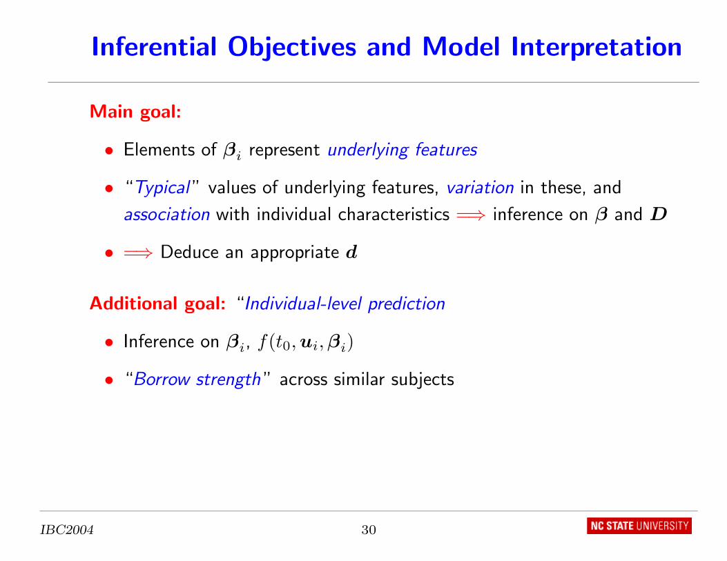
Main goal:

• Elements of βi represent underlying features

• “Typical ” values of underlying features, variation in these, and

association with individual characteristics =⇒ inference on β and D

• =⇒ Deduce an appropriate d

Additional goal: “Individual-level prediction

• Inference on βi, f(t0, ui, βi)

• “Borrow strength ” across similar subjects

IBC2004 30

Inferential Objectives and Model Interpretation

Subject-specific model:

• Not the same as the population averaged approach of modeling

E(yi|zi), var(yi|zi) directly

• Explicitly acknowledges individual behavior

• Interest in the “typical value,” variation of underlying features βi, not

in the “typical response profile” and overall variation about it

• Incorporates scientific assumptions embedded in the model f for

individual behavior

IBC2004 31

Implementation

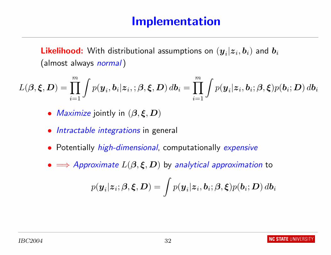
Likelihood: With distributional assumptions on (yi|zi, bi) and bi

(almost always normal )

L(β, ξ, D) =m∏

i=1

∫p(yi, bi|zi, ; β, ξ, D) dbi =

m∏i=1

∫p(yi|zi, bi; β, ξ)p(bi; D) dbi

• Maximize jointly in (β, ξ, D)

• Intractable integrations in general

• Potentially high-dimensional, computationally expensive

• =⇒ Approximate L(β, ξ, D) by analytical approximation to

p(yi|zi; β, ξ, D) =∫

p(yi|zi, bi; β, ξ)p(bi; D) dbi

IBC2004 32

Implementation

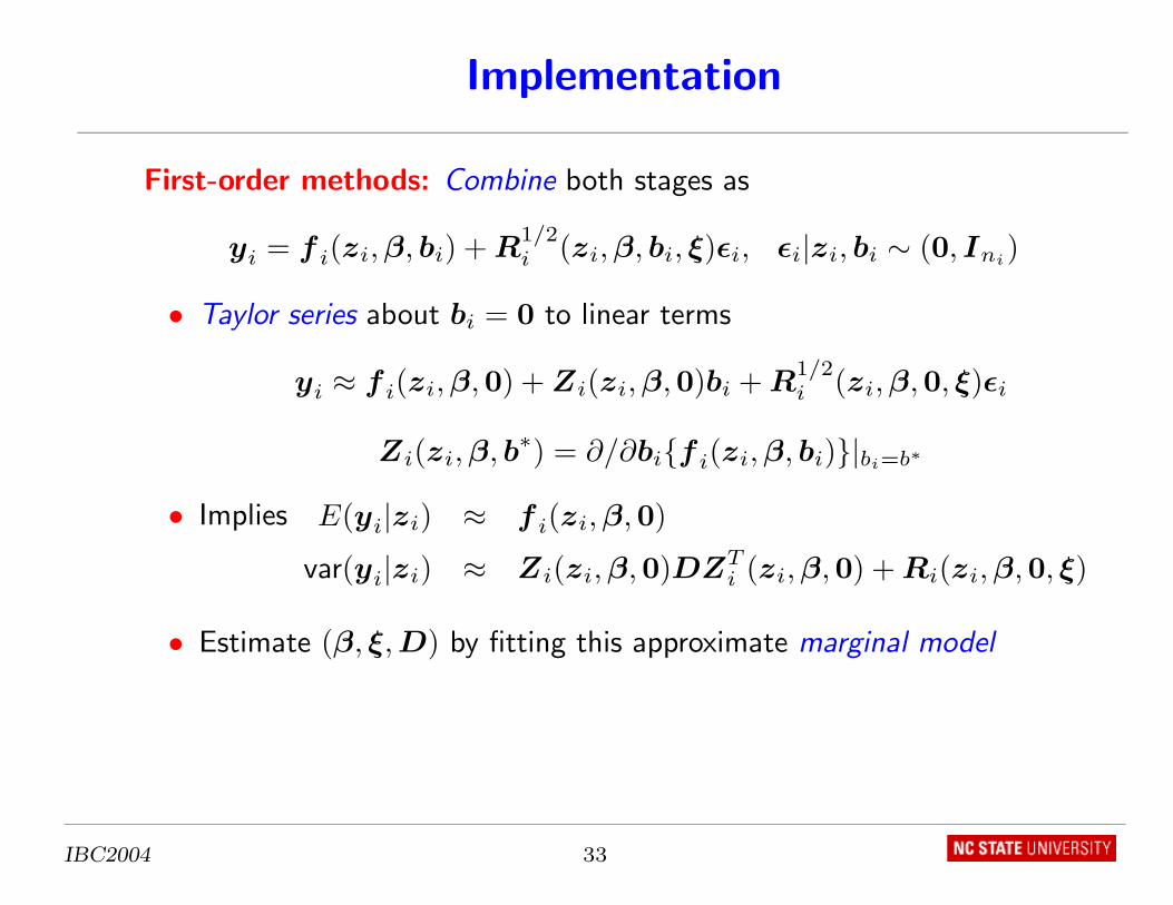
First-order methods: Combine both stages as

yi = f i(zi, β, bi) + R1/2i (zi, β, bi, ξ)εi, εi|zi, bi ∼ (0, Ini

)

• Taylor series about bi = 0 to linear terms

yi ≈ f i(zi, β,0) + Zi(zi, β,0)bi + R1/2i (zi, β,0, ξ)εi

Zi(zi, β, b∗) = ∂/∂bi{f i(zi, β, bi)}|bi=b∗

• Implies E(yi|zi) ≈ f i(zi, β,0)

var(yi|zi) ≈ Zi(zi, β,0)DZTi (zi, β,0) + Ri(zi, β,0, ξ)

• Estimate (β, ξ, D) by fitting this approximate marginal model

IBC2004 33

Implementation

First-order methods: Software

• SAS macro nlinmix with expand=zero – Solve a set of generalized

estimating equations (“GEE-1 ”) based on these marginal moments

• nonmem fo method, SAS proc nlmixed with method=firo –

Maximize normal likelihood with these marginal moments (“GEE-2 ”)

• proc nlmixed cannot handle dependence of Ri on βi, β

• Obvious potential for bias

IBC2004 34

Implementation

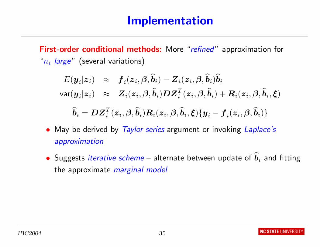
First-order conditional methods: More “refined ” approximation for

“ni large ” (several variations)

E(yi|zi) ≈ f i(zi, β, b̂i)−Zi(zi, β, b̂i)b̂i

var(yi|zi) ≈ Zi(zi, β, b̂i)DZTi (zi, β, b̂i) + Ri(zi, β, b̂i, ξ)

b̂i = DZTi (zi, β, b̂i)Ri(zi, β, b̂i, ξ){yi − f i(zi, β, b̂i)}

• May be derived by Taylor series argument or invoking Laplace’s

approximation

• Suggests iterative scheme – alternate between update of b̂i and fitting

the approximate marginal model

IBC2004 35

Implementation

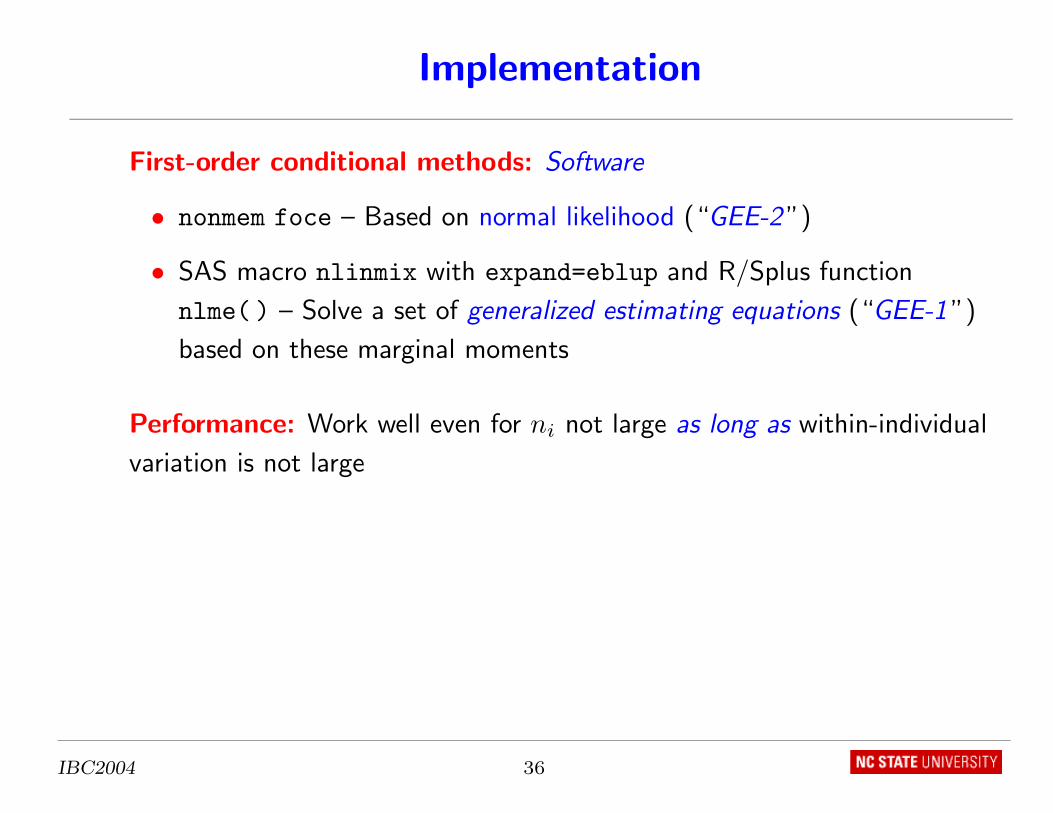
First-order conditional methods: Software

• nonmem foce – Based on normal likelihood (“GEE-2 ”)

• SAS macro nlinmix with expand=eblup and R/Splus function

nlme( ) – Solve a set of generalized estimating equations (“GEE-1 ”)

based on these marginal moments

Performance: Work well even for ni not large as long as within-individual

variation is not large

IBC2004 36

Implementation

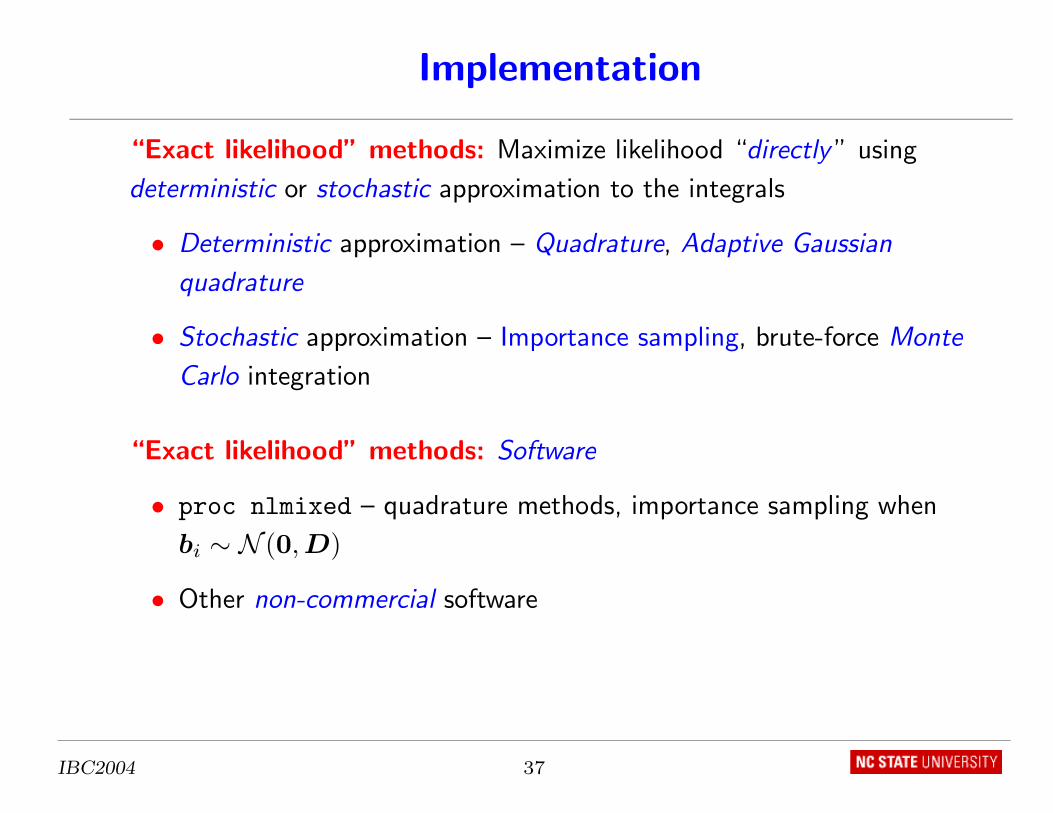
“Exact likelihood” methods: Maximize likelihood “directly ” using

deterministic or stochastic approximation to the integrals

• Deterministic approximation – Quadrature, Adaptive Gaussian

quadrature

• Stochastic approximation – Importance sampling, brute-force Monte

Carlo integration

“Exact likelihood” methods: Software

• proc nlmixed – quadrature methods, importance sampling when

bi ∼ N (0, D)

• Other non-commercial software

IBC2004 37

Implementation

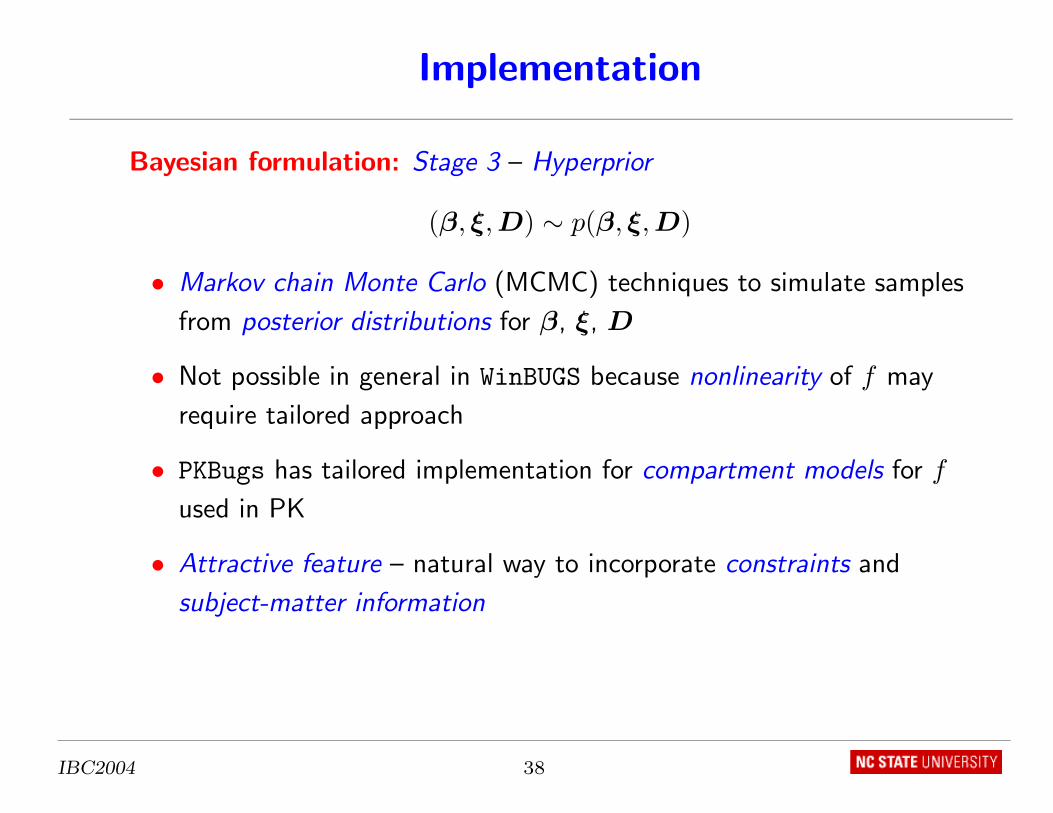
Bayesian formulation: Stage 3 – Hyperprior

(β, ξ, D) ∼ p(β, ξ, D)

• Markov chain Monte Carlo (MCMC) techniques to simulate samples

from posterior distributions for β, ξ, D

• Not possible in general in WinBUGS because nonlinearity of f may

require tailored approach

• PKBugs has tailored implementation for compartment models for f

used in PK

• Attractive feature – natural way to incorporate constraints and

subject-matter information

IBC2004 38

Extensions and Recent Developments

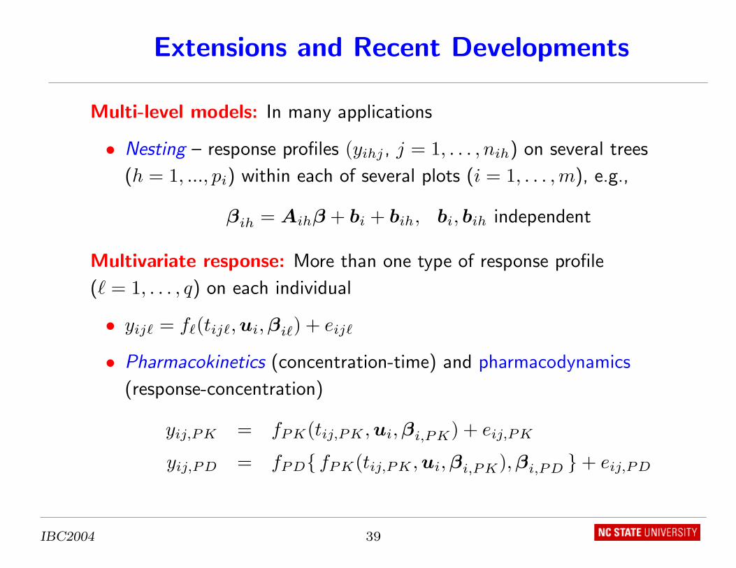
Multi-level models: In many applications

• Nesting – response profiles (yihj , j = 1, . . . , nih) on several trees

(h = 1, ..., pi) within each of several plots (i = 1, . . . , m), e.g.,

βih = Aihβ + bi + bih, bi, bih independent

Multivariate response: More than one type of response profile

(` = 1, . . . , q) on each individual

• yij` = f`(tij`, ui, βi`) + eij`

• Pharmacokinetics (concentration-time) and pharmacodynamics

(response-concentration)

yij,PK = fPK(tij,PK , ui, βi,PK) + eij,PK

yij,PD = fPD{ fPK(tij,PK , ui, βi,PK), βi,PD }+ eij,PD

IBC2004 39

Extensions and Recent Developments

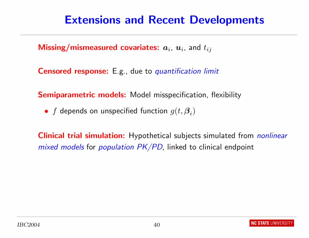
Missing/mismeasured covariates: ai, ui, and tij

Censored response: E.g., due to quantification limit

Semiparametric models: Model misspecification, flexibility

• f depends on unspecified function g(t, βi)

Clinical trial simulation: Hypothetical subjects simulated from nonlinear

mixed models for population PK/PD, linked to clinical endpoint

IBC2004 40

Discussion

• The nonlinear mixed model is now a standard inferential tool used

routinely in many applications

• For extensive references and more details see

Davidian, M. and Giltinan, D.M. (2003), “Nonlinear Models

for Repeated Measurement Data: An Overview and Update,”

JABES 8, 387–419

IBC2004 41