Embed Size (px)
Citation preview
Nonlinear Large Deformation Analysis of RC Bare Frames
Subjected to Lateral Loads
by
Harinadha Babu Raparla, Pradeep Kumar Ramancharla
in
Indian Concrete Institute
Report No: IIIT/TR/2012/-1
Centre for Earthquake EngineeringInternational Institute of Information Technology
Hyderabad - 500 032, INDIAFebruary 2012
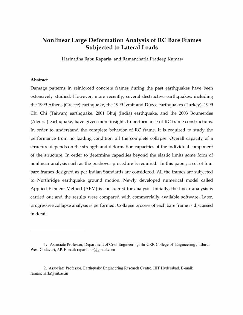
Nonlinear Large Deformation Analysis of RC Bare Frames Subjected to Lateral Loads
Harinadha Babu Raparla1 and Ramancharla Pradeep Kumar2
Abstract
Damage patterns in reinforced concrete frames during the past earthquakes have been
extensively studied. However, more recently, several destructive earthquakes, including
the 1999 Athens (Greece) earthquake, the 1999 Đzmit and Düzce earthquakes (Turkey), 1999
Chi Chi (Taiwan) earthquake, 2001 Bhuj (India) earthquake, and the 2003 Boumerdes
(Algeria) earthquake, have given more insights to performance of RC frame constructions.
In order to understand the complete behavior of RC frame, it is required to study the
performance from no loading condition till the complete collapse. Overall capacity of a
structure depends on the strength and deformation capacities of the individual component
of the structure. In order to determine capacities beyond the elastic limits some form of
nonlinear analysis such as the pushover procedure is required. In this paper, a set of four
bare frames designed as per Indian Standards are considered. All the frames are subjected
to Northridge earthquake ground motion. Newly developed numerical model called
Applied Element Method (AEM) is considered for analysis. Initially, the linear analysis is
carried out and the results were compared with commercially available software. Later,
progressive collapse analysis is performed. Collapse process of each bare frame is discussed
in detail.
1. Associate Professor, Department of Civil Engineering, Sir CRR College of Engineering , Eluru,
West Godavari, AP. E-mail: [email protected]
2. Associate Professor, Earthquake Engineering Research Centre, IIIT Hyderabad. E-mail:
Introduction
A large number of reinforced concrete multi storied framed buildings were heavily
damaged and many of them collapsed completely during earthquakes of the last decade
viz., the 1999 Athens (Greece) earthquake, the 1999 Đzmit and Düzce earthquakes (Turkey),
1999 Chi Chi (Taiwan) earthquake, 2001 Bhuj (India) earthquake, and the 2003 Boumerdes
(Algeria) earthquake. These damages have clearly shown strengths of the structure to give
ground motion. Strength of a structure mainly depends on deformation capacities of the
individual component of the structure. In order to determine capacities beyond the elastic
limits some form of nonlinear analysis such as the pushover procedure is required. Usually
seismic demands are computed by nonlinear static analysis of the structure, which is
subjected to monotonically increasing lateral forces with an invariant height-wise
distribution until a target displacement is reached. However, clear understanding of the
performance under critical dynamic loading cannot be understood by this procedure. For
this purpose, we need to use highly efficient numerical modeling procedures.
Simulation of such a behavior is not an easy job using currently available numerical
techniques. Currently available numerical methods for structural analysis can be classified
into two categories. In the first category, model is based on continuum material equations.
The finite element method (FEM) is typical example of this category. The mathematical
model of the structure is modified to account for reduced resistance of yielding
components. For two dimensional models computer programs are available that directly
model nonlinear behavior efficiently in static way and to some reasonable level of accuracy
in dynamic way. However, to perform collapse far exceeding their elastic limit is a difficult
task to many numerical methods. Currently there are several limitations in adopting this
approach. For example in high nonlinear case where crack has initiated and element is not
detached from the structure, smeared crack approach is followed. However, smeared Crack
approach cannot be adopted in zones where separation occurs between adjacent structural
elements. While, Discrete Crack Methods assume that the location and direction of crack
propagation are predefined before the analysis. With this group of the methods, analysis of
structures, especially concrete structures, can be performed at most before collapse. The
second category of methods uses the discrete element techniques, like the Rigid Body and
Spring Model (RBSM)7)and Modified or Extended Distinct Element Method, (MDEM or
EDEM) 8) The main advantage of these methods is that they can simulate the cracking
process with relatively simple technique compared to the FEM, while the main
disadvantage is that crack propagation depends mainly on the element shape, size and
arrangement. Analysis using the RBSM could not be performed up to complete collapse of
the structure. On the other hand, the EDEM can follow the structural behavior from zero
loading and up to complete collapse of the structure. However, the accuracy of EDEM in
small deformation range is less than that of the FEM. Hence, the failure behavior obtained
by repeated many calculations is affected due to cumulative errors and cannot be predicted
accurately using the EDEM. However, AEM has the capability of simulating behavior of
structures from zero loading to collapse can be followed with reliable accuracy, reasonable
CPU time and with relatively simple material models. Hence in this research, numerical
simulation is performed with Applied Element Method (AEM).
The major advantages of the Applied Element Method (AEM) are simple modeling and
programming and high accuracy of the results with relatively short CPU time. Using the
AEM, highly nonlinear behavior, i.e. crack initiation, crack propagation, separation of
structural elements, rigid body motion of failed elements and collapse process of the
structure can be followed with high accuracy. In this paper, AEM is used to perform the
analysis.
Overview of the Numerical Method
In this research numerical simulation is performed with applied element method. In AEM 1,
2 ) structure is modeled as an assembly of small elements which is made by dividing of the
structure virtually, as shown in figure 1. The two elements shown in figure 1 are assumed
to be connected by pairs of normal and shear springs located at contact points which are
distributed around the element edges. Each pair of springs totally represents stresses and
deformations of a certain area (hatched area in figure.1b) of the studied elements. The
spring stiffness is determined as shown in equation.1
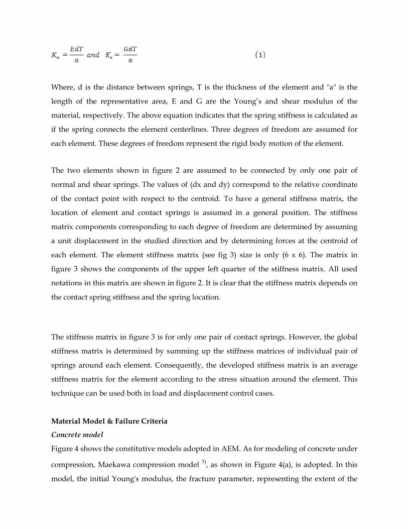
Where, d is the distance between springs, T is the thickness of the element and "a" is the
length of the representative area, E and G are the Young’s and shear modulus of the
material, respectively. The above equation indicates that the spring stiffness is calculated as
if the spring connects the element centerlines. Three degrees of freedom are assumed for
each element. These degrees of freedom represent the rigid body motion of the element.
The two elements shown in figure 2 are assumed to be connected by only one pair of
normal and shear springs. The values of (dx and dy) correspond to the relative coordinate
of the contact point with respect to the centroid. To have a general stiffness matrix, the
location of element and contact springs is assumed in a general position. The stiffness
matrix components corresponding to each degree of freedom are determined by assuming
a unit displacement in the studied direction and by determining forces at the centroid of
each element. The element stiffness matrix (see fig 3) size is only (6 x 6). The matrix in
figure 3 shows the components of the upper left quarter of the stiffness matrix. All used
notations in this matrix are shown in figure 2. It is clear that the stiffness matrix depends on
the contact spring stiffness and the spring location.
The stiffness matrix in figure 3 is for only one pair of contact springs. However, the global
stiffness matrix is determined by summing up the stiffness matrices of individual pair of
springs around each element. Consequently, the developed stiffness matrix is an average
stiffness matrix for the element according to the stress situation around the element. This
technique can be used both in load and displacement control cases.
Material Model & Failure Criteria
Concrete model
Figure 4 shows the constitutive models adopted in AEM. As for modeling of concrete under
compression, Maekawa compression model 3), as shown in Figure 4(a), is adopted. In this
model, the initial Young's modulus, the fracture parameter, representing the extent of the
internal damage of concrete and the compressive plastic strain are introduced to define the
envelope for compressive stresses and compressive strains. Therefore unloading and
reloading can be conveniently described. The tangent modulus is calculated according to
the strain at the spring location. After peak stresses, spring stiffness is assumed as a
minimum value (1% of initial value) to avoid negative stiffness. This results in difference
between calculated stress and stress corresponds to the spring strain. These residual
stresses are redistributed by applying the redistributed force values in the reverse direction
in the next loading step.
For concrete springs subjected to tension, spring stiffness is assumed as the initial stiffness
until reaching the cracking point. After cracking, stiffness of springs subjected to tension is
set to be zero. The residual stresses are then redistributed in the next loading step by
applying the redistributed force values in the reverse direction. For concrete springs, the
relationship between shear stress and shear strain is assumed to remain linear till the
cracking of concrete. Then, the shear stresses drop down as shown in figure 4(b). The level
of drop of shear stresses depends on the aggregate interlock and friction at the crack
surface.
Reinforcing bars Model
For reinforcement springs, the model presented by Ristic et al.4) is used and it is shown in
Figure 5. The tangent stiffness of reinforcement is calculated based on the strain from the
reinforcement spring, loading status (either loading or unloading) and the previous history
of steel spring which controls the Bauschinger's effect.
The main advantage of this model is that it can consider easily the effects of partial
unloading and Baushinger's effect without any additional complications to the analysis.
After reaching 10% tensile strain, it is assumed that the reinforcement bar is cut. The force
carried by the reinforcement bar is redistributed, when it reaches the failure criterion 2) by
applying the redistributed force to the corresponding elements in the reverse direction.
Small deformation vs large deformation
Even though the analysis to be performed is dynamic, equations remain same in both static
as well as dynamic cases except for inertia and damping terms.
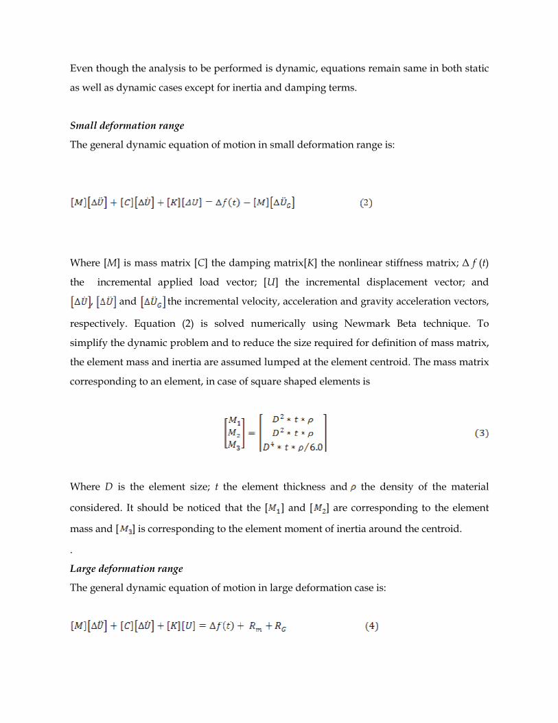
Small deformation range
The general dynamic equation of motion in small deformation range is:
Where [M] is mass matrix [C] the damping matrix[K] the nonlinear stiffness matrix; ∆ f (t)
the incremental applied load vector; [U] the incremental displacement vector; and
, and the incremental velocity, acceleration and gravity acceleration vectors,
respectively. Equation (2) is solved numerically using Newmark Beta technique. To
simplify the dynamic problem and to reduce the size required for definition of mass matrix,
the element mass and inertia are assumed lumped at the element centroid. The mass matrix
corresponding to an element, in case of square shaped elements is
Where D is the element size; t the element thickness and the density of the material
considered. It should be noticed that the [ ] and [ ] are corresponding to the element
mass and [ ] is corresponding to the element moment of inertia around the centroid.
.
Large deformation range
The general dynamic equation of motion in large deformation case is:
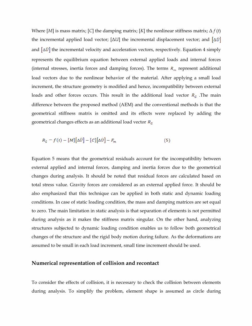
Where [M] is mass matrix; [C] the damping matrix; [K] the nonlinear stiffness matrix; ∆ f (t)
the incremental applied load vector; [∆U] the incremental displacement vector; and
and the incremental velocity and acceleration vectors, respectively. Equation 4 simply
represents the equilibrium equation between external applied loads and internal forces
(internal stresses, inertia forces and damping forces). The terms represent additional
load vectors due to the nonlinear behavior of the material. After applying a small load
increment, the structure geometry is modified and hence, incompatibility between external
loads and other forces occurs. This result in the additional load vector .The main
difference between the proposed method (AEM) and the conventional methods is that the
geometrical stiffness matrix is omitted and its effects were replaced by adding the
geometrical changes effects as an additional load vector
Equation 5 means that the geometrical residuals account for the incompatibility between
external applied and internal forces, damping and inertia forces due to the geometrical
changes during analysis. It should be noted that residual forces are calculated based on
total stress value. Gravity forces are considered as an external applied force. It should be
also emphasized that this technique can be applied in both static and dynamic loading
conditions. In case of static loading condition, the mass and damping matrices are set equal
to zero. The main limitation in static analysis is that separation of elements is not permitted
during analysis as it makes the stiffness matrix singular. On the other hand, analyzing
structures subjected to dynamic loading condition enables us to follow both geometrical
changes of the structure and the rigid body motion during failure. As the deformations are
assumed to be small in each load increment, small time increment should be used.
Numerical representation of collision and recontact
To consider the effects of collision, it is necessary to check the collision between elements
during analysis. To simplify the problem, element shape is assumed as circle during
collision. This assumption is acceptable if the element size is relatively small. Even in case
of relatively large elements used, it may be reasonable because in the deformation range of
collision, the sharp corners of elements are broken due to the stress concentration and the
edge of the elements become round shape. Based on the assumptions, only distance
between the centres of the elements is calculated to check collision 5)
Contact and collision forces are considered in the analysis through collision springs, which
are added at the locations where collision or recontact between elements occurs. The effects
of separation, recontact and collision can be considered easily with high accuracy and
without large increase of the CPU time. The main advantage of the proposed technique
compared to the Extended Distinct Element Method (EDEM) is that the time increment can
be much larger than the EDEM.
Calculation of Time Step
Time effects are continuous since the start of loading till the end of analysis. As the
nonlinear dynamic phenomenon is very complicated to be solved using exact solutions,
approximate numerical solution for the dynamic equation is adopted. The numerical
solution is based on assumption of a small time step that can follow the structural behavior.
The selection of the time step is very important. Having too short a time step will result in
very long analysis time. Using a large time step thus a short analysis time will result in less
accurate analysis. The numerical solution may fail to converge if the selected time step is
large. Say that the time step is ∆T, and then the shortest period that can be considered in the
analysis is 2∆T. Thus all the frequencies higher than that will not affect the analysis 6)
The applied excitation is applied as a record with a recording time step. For calculation
purposes, the recording time step is subdivided into smaller steps called calculation time
steps. The ratio of recording calculation time step is usually bigger than unity. The bigger
ratio is the better the accuracy and the convergence of results. Earthquakes usually requires
time step as 0.001 to 0.01 sec for analysis. When collision is expected to occur, the time step
should be less than the contact time between elements to have good contact relations.
Case Studies
For the purpose of this study, we selected four bare frames viz., single storey-single bay,
three storey-one bay, five storey-one bay and ten storey-three bay as shown in the figures
8a, 9a, 10a and 11a respectively. Storey heights and bay widths are considered constant i.e.,
4.0 m and 3.9 m respectively in the entire one bay structure. All these two dimensional RC
bare frames, are designed to withstand normal gravity and lateral loads as per IS codes.
Design has considered all the frames as ordinary moment resisting frames. These bare RC
frames of different stories are modeled with reinforcement and appropriate materials for
the simulation. The numerical simulation is performed with applied element method
(AEM). Column and beam sizes are fixed as 0.3m×0.3m. Longitudinal and lateral
reinforcement details of all the one bay frames are taken from the designs obtained as per IS
codes. For numerical modeling element size is taken as constant i.e., 100mm×100mm for all
the one bay frames. For ten storey- three bay frame Storey heights and each bay width(c/c)
are taken as 4.2m and 7.8m respectively. Column and beam sizes are fixed as 600mm ×
600mm and 300mm × 600mm respectively for all the floors of ten storey frame.
Longitudinal and lateral reinforcement details of ten storey frame are taken from designs
obtained as per IS codes. For numerical modeling element size is taken as constant i.e.,
300mm × 300mm for ten storey -three bay frames. Material properties used in the analysis
are described in table 1. Damping value is taken as 5%.
Initially, eigen value analysis is performed for finding the natural frequencies and mode
shapes of the structure. Fundamental natural periods of four structures are 61.05, 17.92,
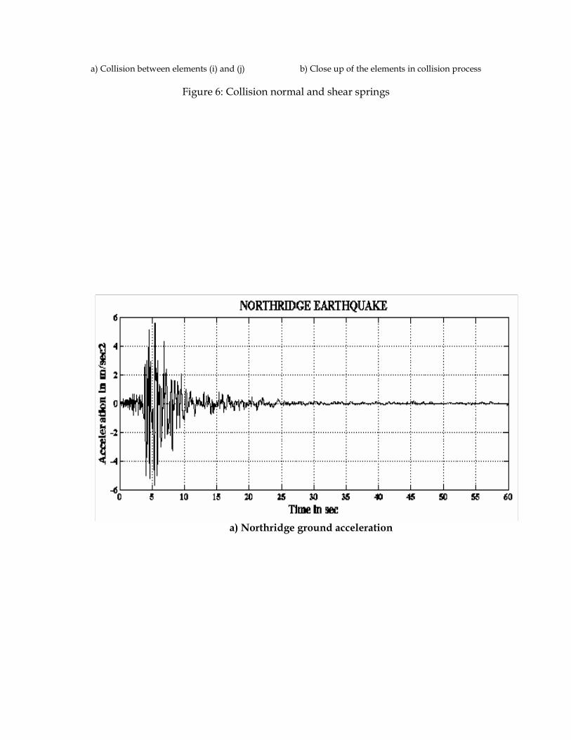
10.12 and 6.04 rad/sec respectively. For performing dynamic analysis, Northridge
earthquake has been considered. Ground motion time history and Fourier amplitude
spectrum of the earthquake are shown in the figures 7 a and b. From the figure 7a it can be
seen that the ground motion has PGA at around 5 sec and from figure 7b predominant
frequencies range from 1 to 4 hz. Hence, the structures falling in that frequency band will
have maximum displacement amplitude.
In dynamic analysis, first linear analysis is performed. The responses obtained by AEM
simulations are studied and compared with the results of other software for the
verification. The results of dynamic linear analysis are in agreement with SAP-2000 9) and
STAAD 10) package results. Secondly, nonlinear dynamic analysis is performed by giving
Northridge earthquake ground motion. Details of these cases are described below.
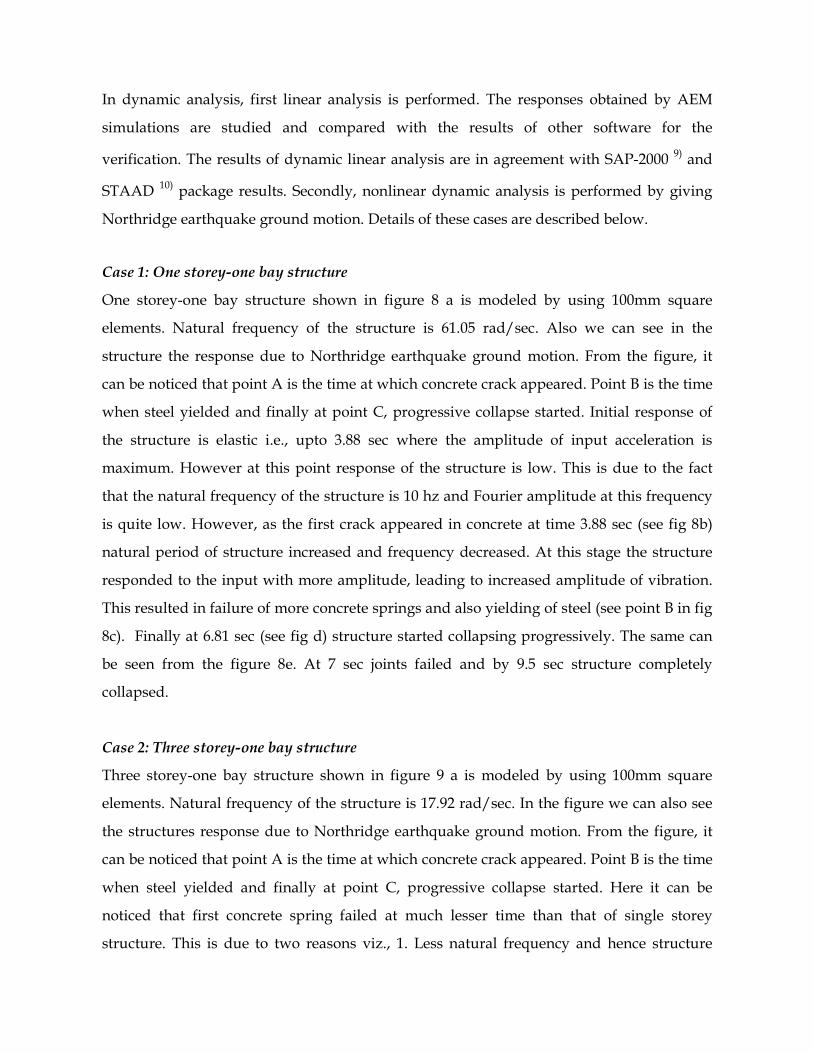
Case 1: One storey-one bay structure
One storey-one bay structure shown in figure 8 a is modeled by using 100mm square
elements. Natural frequency of the structure is 61.05 rad/sec. Also we can see in the
structure the response due to Northridge earthquake ground motion. From the figure, it
can be noticed that point A is the time at which concrete crack appeared. Point B is the time
when steel yielded and finally at point C, progressive collapse started. Initial response of
the structure is elastic i.e., upto 3.88 sec where the amplitude of input acceleration is
maximum. However at this point response of the structure is low. This is due to the fact
that the natural frequency of the structure is 10 hz and Fourier amplitude at this frequency
is quite low. However, as the first crack appeared in concrete at time 3.88 sec (see fig 8b)
natural period of structure increased and frequency decreased. At this stage the structure
responded to the input with more amplitude, leading to increased amplitude of vibration.
This resulted in failure of more concrete springs and also yielding of steel (see point B in fig
8c). Finally at 6.81 sec (see fig d) structure started collapsing progressively. The same can
be seen from the figure 8e. At 7 sec joints failed and by 9.5 sec structure completely
collapsed.
Case 2: Three storey-one bay structure
Three storey-one bay structure shown in figure 9 a is modeled by using 100mm square
elements. Natural frequency of the structure is 17.92 rad/sec. In the figure we can also see
the structures response due to Northridge earthquake ground motion. From the figure, it
can be noticed that point A is the time at which concrete crack appeared. Point B is the time
when steel yielded and finally at point C, progressive collapse started. Here it can be
noticed that first concrete spring failed at much lesser time than that of single storey
structure. This is due to two reasons viz., 1. Less natural frequency and hence structure
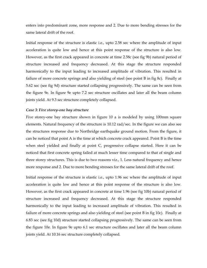
enters into predominant zone, more response and 2. Due to more bending stresses for the
same lateral drift of the roof.
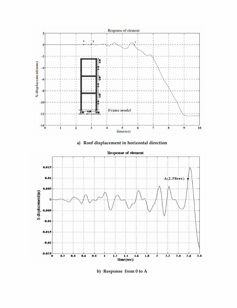
Initial response of the structure is elastic i.e., upto 2.58 sec where the amplitude of input
acceleration is quite low and hence at this point response of the structure is also low.
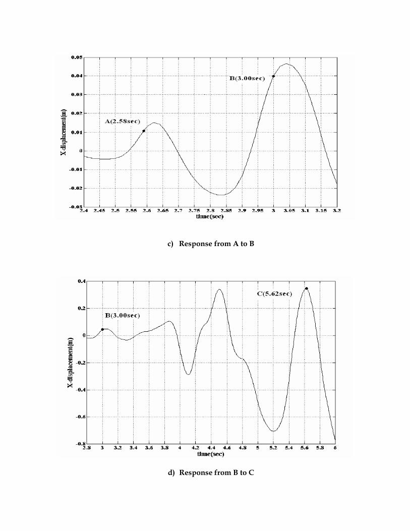
However, as the first crack appeared in concrete at time 2.58c (see fig 9b) natural period of
structure increased and frequency decreased. At this stage the structure responded
harmonically to the input leading to increased amplitude of vibration. This resulted in
failure of more concrete springs and also yielding of steel (see point B in fig 8c). Finally at
5.62 sec (see fig 9d) structure started collapsing progressively. The same can be seen from
the figure 9e. In figure 9e upto 7.2 sec structure oscillates and later all the beam column
joints yield. At 9.3 sec structure completely collapsed.
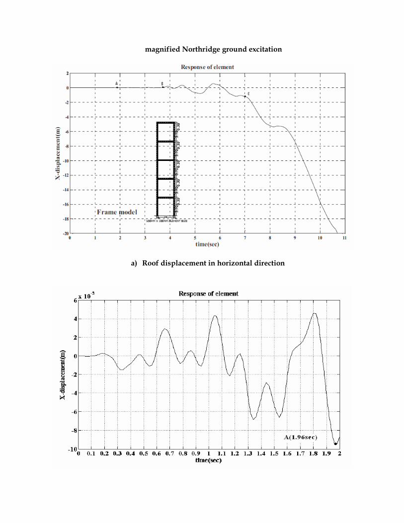
Case 3: Five storey-one bay structure
Five storey-one bay structure shown in figure 10 a is modeled by using 100mm square
elements. Natural frequency of the structure is 10.12 rad/sec. In the figure we can also see
the structures response due to Northridge earthquake ground motion. From the figure, it
can be noticed that point A is the time at which concrete crack appeared. Point B is the time
when steel yielded and finally at point C, progressive collapse started. Here it can be
noticed that first concrete spring failed at much lesser time compared to that of single and
three storey structures. This is due to two reasons viz., 1. Less natural frequency and hence
more response and 2. Due to more bending stresses for the same lateral drift of the roof.
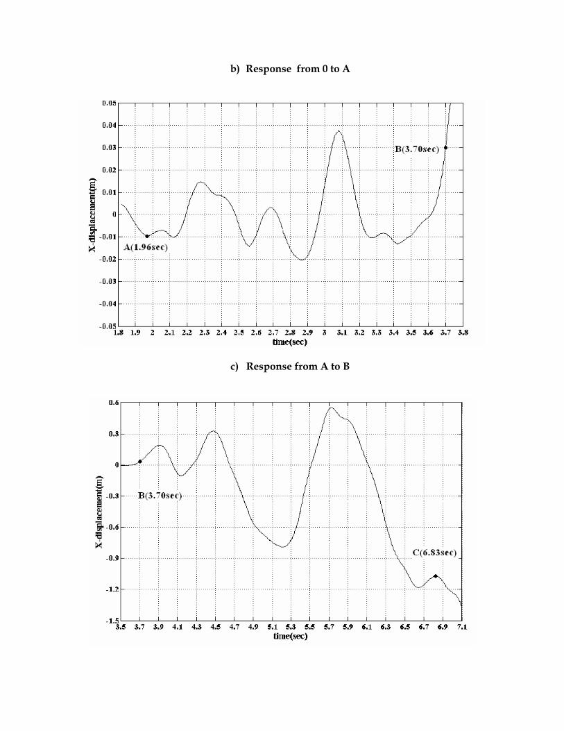
Initial response of the structure is elastic i.e., upto 1.96 sec where the amplitude of input
acceleration is quite low and hence at this point response of the structure is also low.
However, as the first crack appeared in concrete at time 1.96 (see fig 10b) natural period of
structure increased and frequency decreased. At this stage the structure responded
harmonically to the input leading to increased amplitude of vibration. This resulted in
failure of more concrete springs and also yielding of steel (see point B in fig 10c). Finally at
6.83 sec (see fig 10d) structure started collapsing progressively. The same can be seen from
the figure 10e. In figure 9e upto 6.1 sec structure oscillates and later all the beam column
joints yield. At 10.16 sec structure completely collapsed.
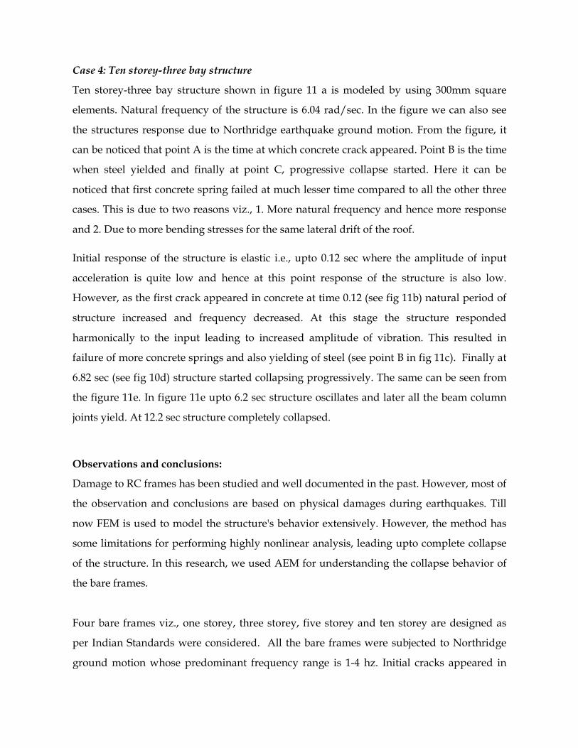
Case 4: Ten storey-three bay structure
Ten storey-three bay structure shown in figure 11 a is modeled by using 300mm square
elements. Natural frequency of the structure is 6.04 rad/sec. In the figure we can also see
the structures response due to Northridge earthquake ground motion. From the figure, it
can be noticed that point A is the time at which concrete crack appeared. Point B is the time
when steel yielded and finally at point C, progressive collapse started. Here it can be
noticed that first concrete spring failed at much lesser time compared to all the other three
cases. This is due to two reasons viz., 1. More natural frequency and hence more response
and 2. Due to more bending stresses for the same lateral drift of the roof.
Initial response of the structure is elastic i.e., upto 0.12 sec where the amplitude of input
acceleration is quite low and hence at this point response of the structure is also low.
However, as the first crack appeared in concrete at time 0.12 (see fig 11b) natural period of
structure increased and frequency decreased. At this stage the structure responded
harmonically to the input leading to increased amplitude of vibration. This resulted in
failure of more concrete springs and also yielding of steel (see point B in fig 11c). Finally at
6.82 sec (see fig 10d) structure started collapsing progressively. The same can be seen from
the figure 11e. In figure 11e upto 6.2 sec structure oscillates and later all the beam column
joints yield. At 12.2 sec structure completely collapsed.
Observations and conclusions:
Damage to RC frames has been studied and well documented in the past. However, most of
the observation and conclusions are based on physical damages during earthquakes. Till
now FEM is used to model the structure's behavior extensively. However, the method has
some limitations for performing highly nonlinear analysis, leading upto complete collapse
of the structure. In this research, we used AEM for understanding the collapse behavior of
the bare frames.
Four bare frames viz., one storey, three storey, five storey and ten storey are designed as
per Indian Standards were considered. All the bare frames were subjected to Northridge
ground motion whose predominant frequency range is 1-4 hz. Initial cracks appeared in
concrete first, as the height of the structure is increasing. It means that three storey structure
yielded first compared to single storey structure. It can be clearly understood that
predominant frequency of the singly storey structure is away from resonating frequency of
the ground motion compared to three storey building. Also, as the structure vibrates, more
bending stresses are likely to develop in taller structure due to same drift compared to
shorter structure. This phenomenon is clearly seen in all the bare frames. Even after the first
yield, resistance was offered, as steel in resisting dominantly the flexural tension. Once the
re-bars started failing, stiffness reduced significantly. Since all the structures are
indeterminate structures, capacity is high. All the structures predominantly behaved in
bending mode. However, as the steel bars were cut, then the progressive collapse phase
started in the frames. It started in single storey frame at 6.7 sec, in three storey frame at 5.8
sec, in five storey frame at 7 sec and in ten storey frame at 6.8 sec. From the above, it can be
concluded that the progressive collapse can be studied by AEM, starting from no loading
upto complete collapse.
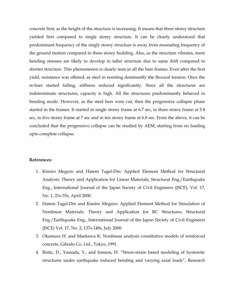
References:
1. Kimiro Meguro and Hatem Tagel-Din: Applied Element Method for Structural
Analysis: Theory and Application for Linear Materials, Structural Eng./Earthquake
Eng., International Journal of the Japan Society of Civil Engineers (JSCE), Vol. 17,
No. 1, 21s-35s, April 2000.
2. Hatem Tagel-Din and Kimiro Meguro: Applied Element Method for Simulation of
Nonlinear Materials: Theory and Application for RC Structures, Structural
Eng./Earthquake Eng., International Journal of the Japan Society of Civil Engineers
(JSCE) Vol. 17, No. 2, 137s-148s, July 2000.
3. Okamura H. and Maekawa K: Nonlinear analysis constitutive models of reinforced
concrete, Gihodo Co. Ltd., Tokyo, 1991.
4. Ristic, D., Yamada, Y., and Iemura, H. “Stress-strain based modeling of hysteretic
structures under earthquake induced bending and varying axial loads”, Research
report No. 86-ST-01, School of Civil Engineering, Kyoto University, Kyoto,
Japan,1986
5. Hatem Tagel-Din: Collision of Structures during Earthquakes, Proceedings of the
12th European Conference on Earthquake Engineering, London, UK, September 9th -
September 13th, 2002.
6. Extreme Loading for Structures Technical Manual,ASI,2006
7. Kawai T Recent developments of the Rigid Body and Spring Model (RBSM) in
structural analysis, Seiken Seminar Text Book, Institute of Industrial Science, The
University of Tokyo, pp. 226-237, 1986.
8. Meguro K. and Hakuno M: Fracture analyses of structures by the modified distinct
element method, Structural Eng./Earthquake Eng., Vol. 6. No. 2, 283s-294s., Japan
Society of Civil Engineers, 1989.
9. SAP2000, Version Advanced 11.0.0, “Structural Analysis Program,” Computers and Structures Inc., 2000.
10. STAAD Pro, general-purpose structural analysis and design solution, Bentley California, USA, 2006.
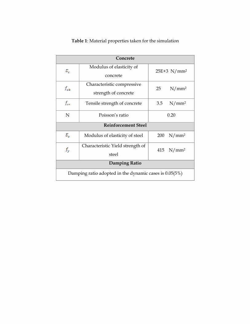
Table 1: Material properties taken for the simulation
Concrete
Modulus of elasticity of
concrete 25E+3 N/mm2
Characteristic compressive
strength of concrete 25 N/mm2
Tensile strength of concrete 3.5 N/mm2
Ν Poisson’s ratio 0.20
Reinforcement Steel
Modulus of elasticity of steel 200 N/mm2
Characteristic Yield strength of
steel 415 N/mm2
Damping Ratio
Damping ratio adopted in the dynamic cases is 0.05(5%)
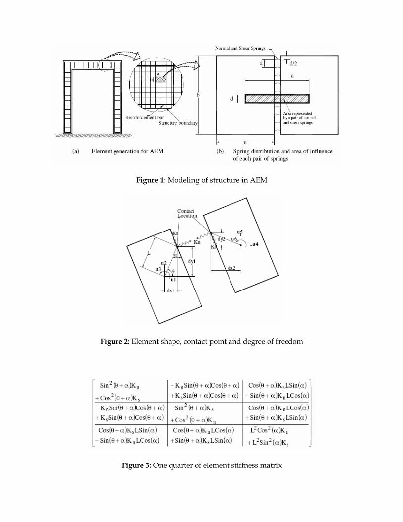
Figure 1: Modeling of structure in AEM
Figure 2: Element shape, contact point and degree of freedom
Figure 3: One quarter of element stiffness matrix
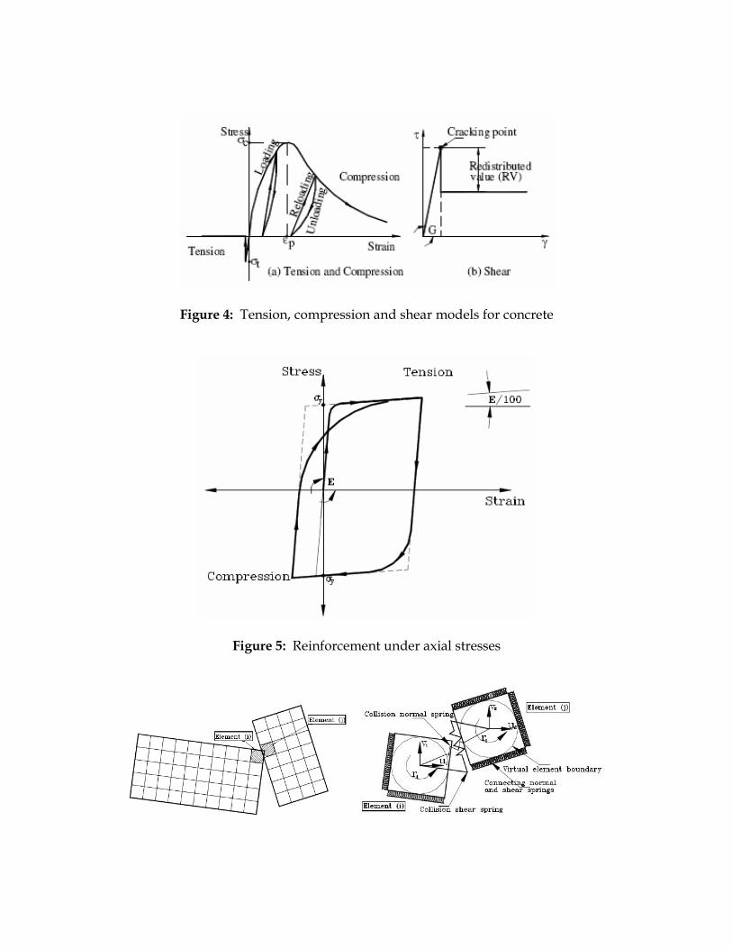
Figure 4: Tension, compression and shear models for concrete
Figure 5: Reinforcement under axial stresses
a) Collision between elements (i) and (j) b) Close up of the elements in collision process
Figure 6: Collision normal and shear springs
a) Northridge ground acceleration
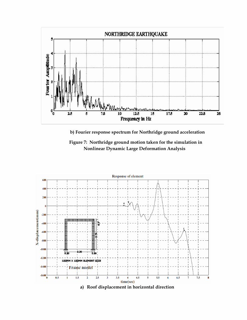
b) Fourier response spectrum for Northridge ground acceleration
Figure 7: Northridge ground motion taken for the simulation in
Nonlinear Dynamic Large Deformation Analysis
a) Roof displacement in horizontal direction
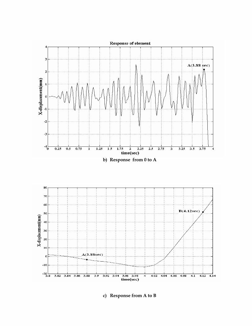
b) Response from 0 to A
c) Response from A to B
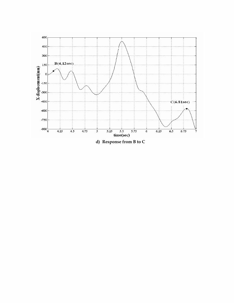
d) Response from B to C
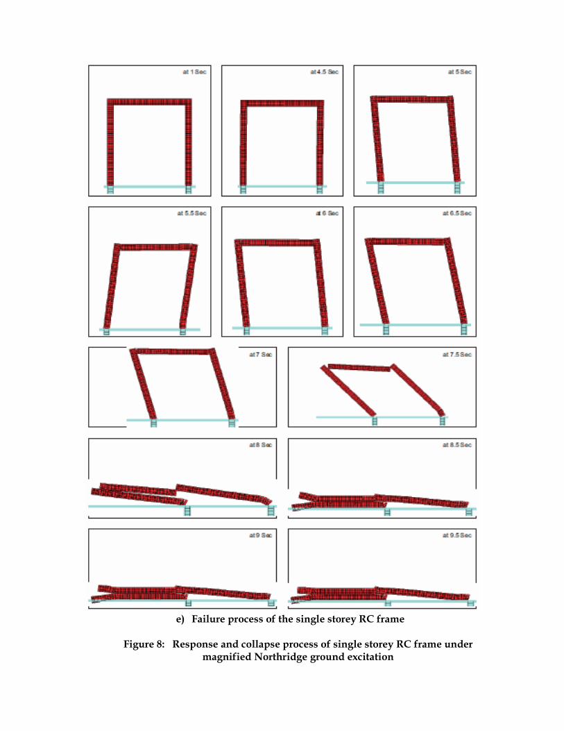
e) Failure process of the single storey RC frame
Figure 8: Response and collapse process of single storey RC frame under
magnified Northridge ground excitation
a) Roof displacement in horizontal direction
b) Response from 0 to A
c) Response from A to B
d) Response from B to C
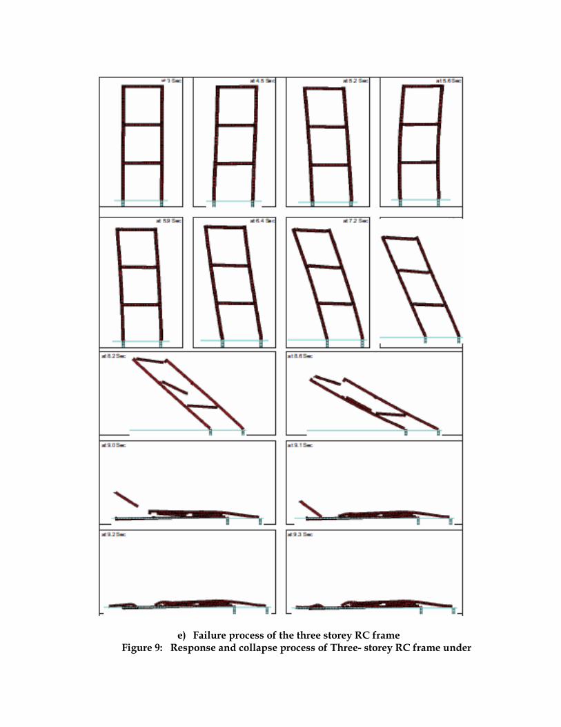
e) Failure process of the three storey RC frame Figure 9: Response and collapse process of Three- storey RC frame under
magnified Northridge ground excitation
a) Roof displacement in horizontal direction
b) Response from 0 to A
c) Response from A to B

d) Response from B to C
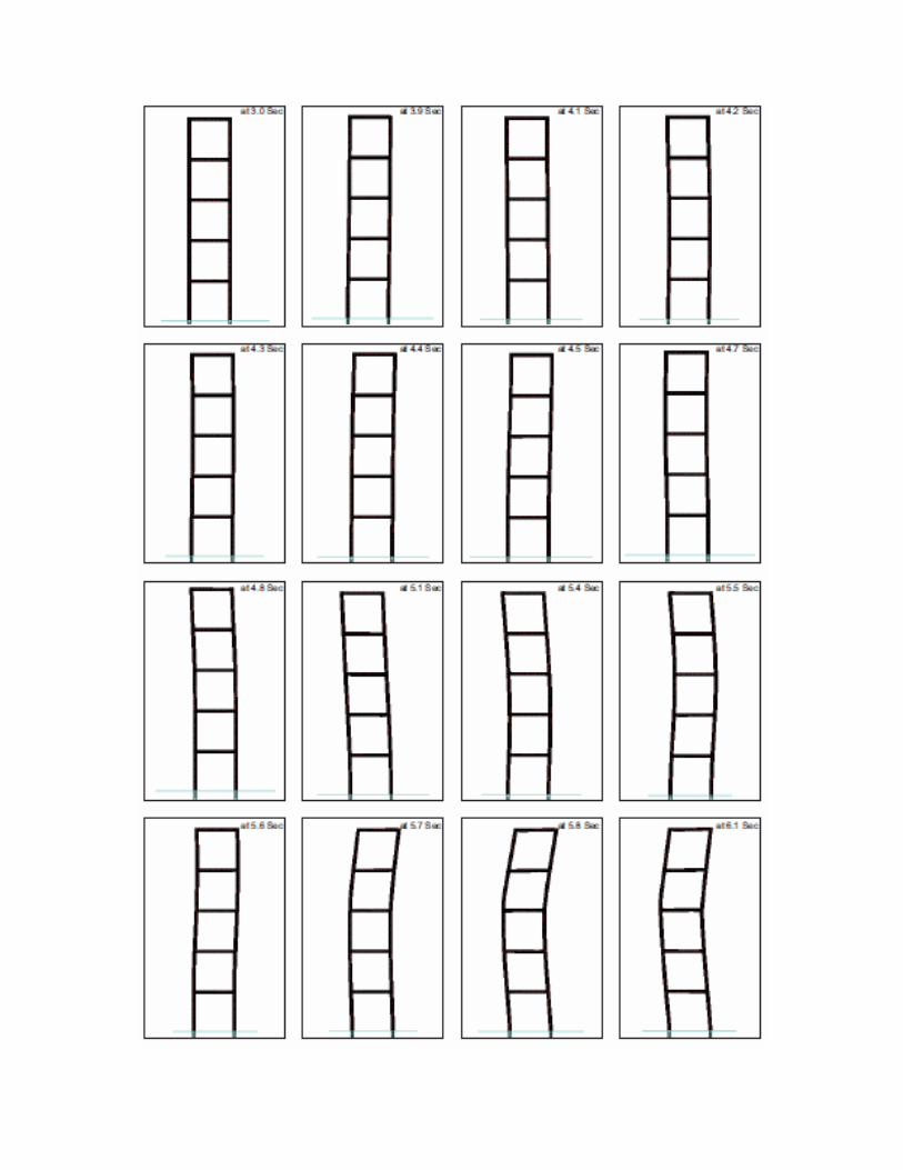
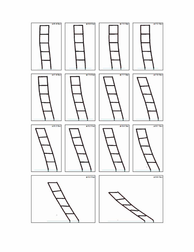
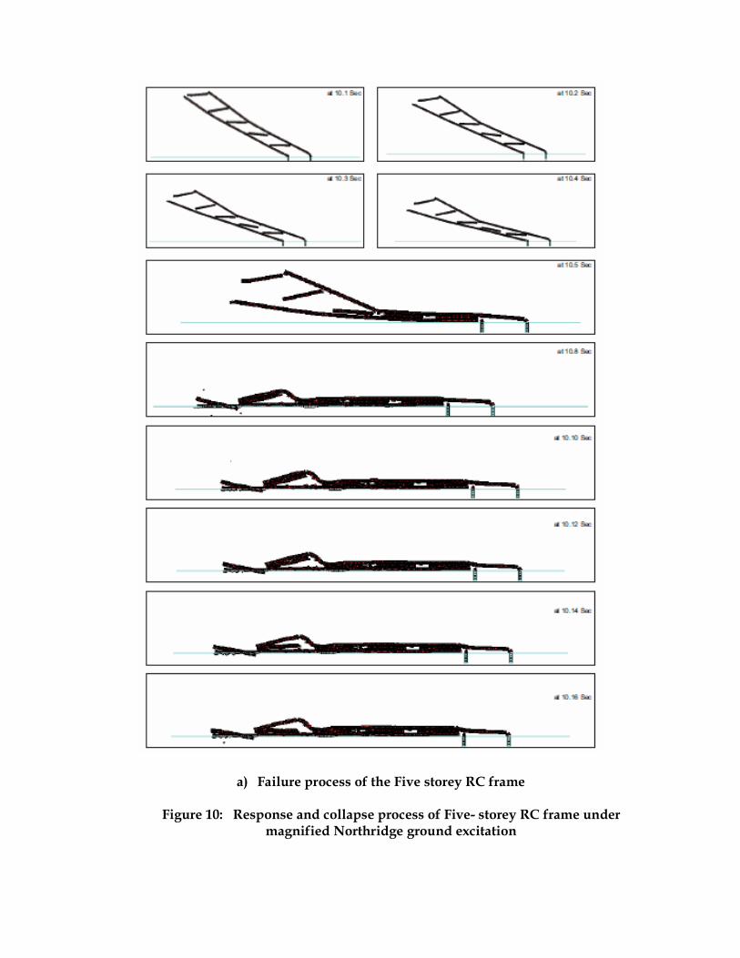
a) Failure process of the Five storey RC frame
Figure 10: Response and collapse process of Five- storey RC frame under magnified Northridge ground excitation
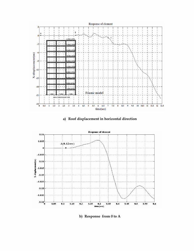
a) Roof displacement in horizontal direction
b) Response from 0 to A
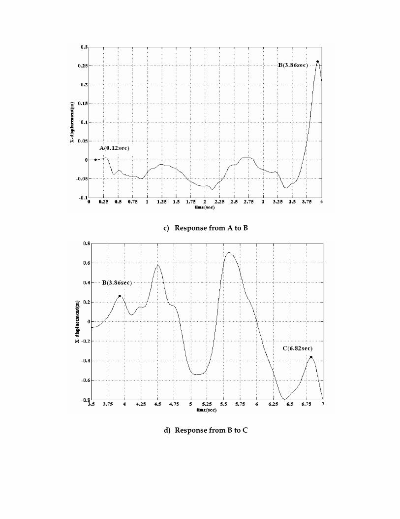
c) Response from A to B
d) Response from B to C
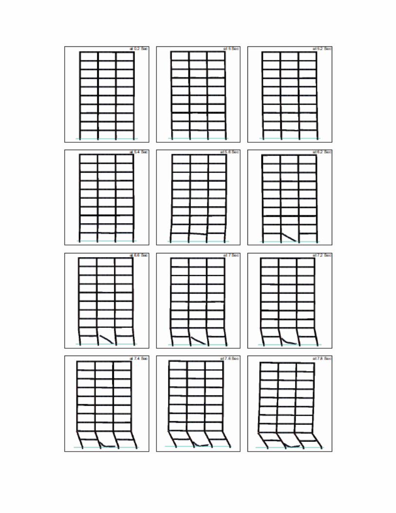
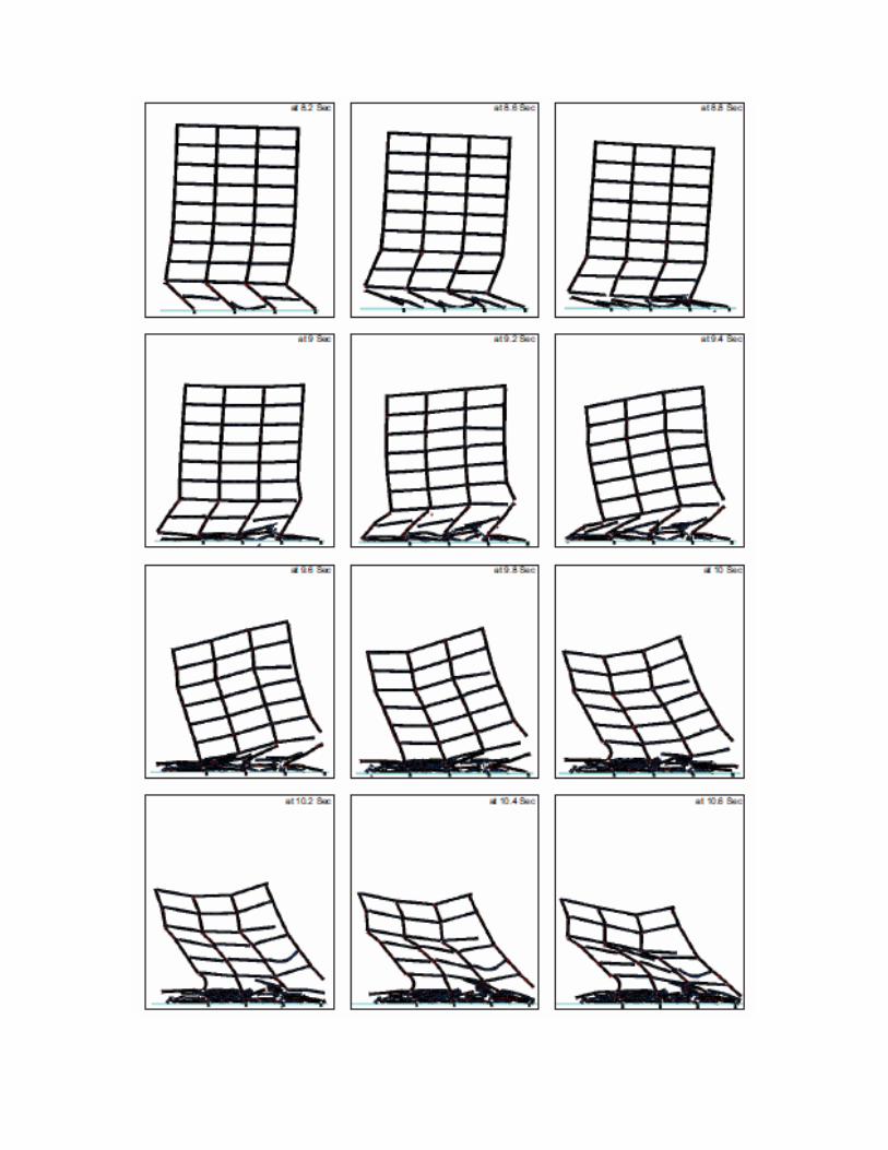
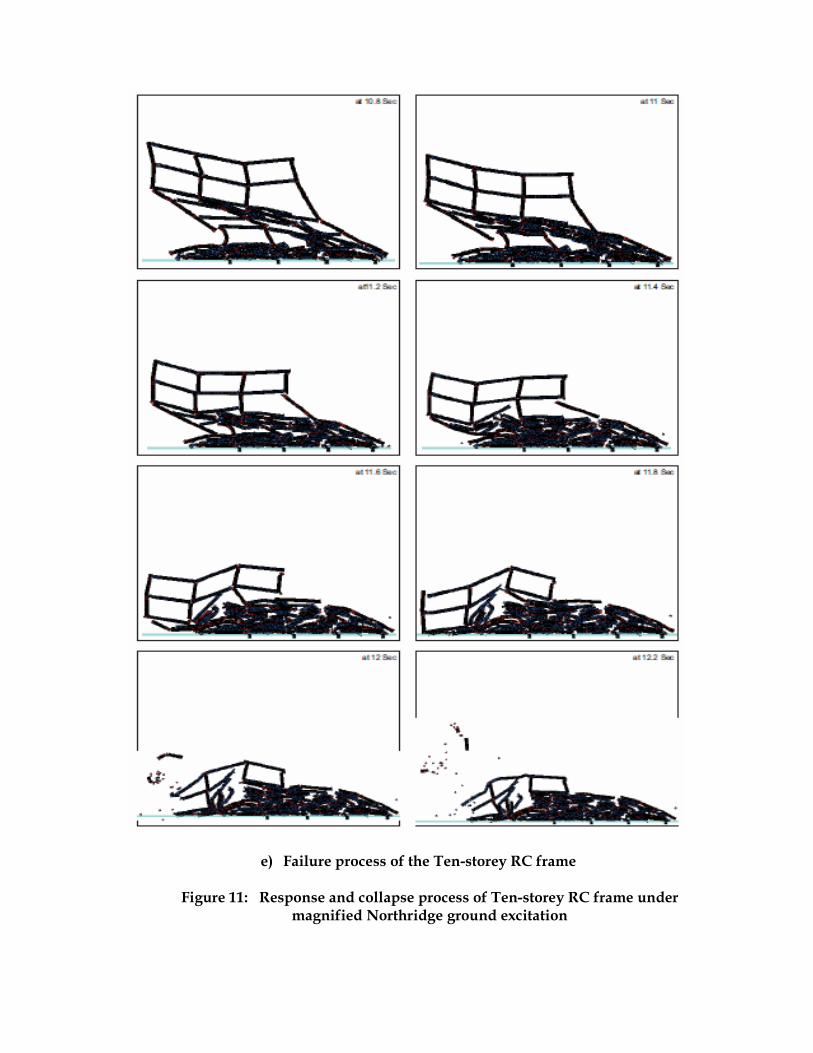
e) Failure process of the Ten-storey RC frame
Figure 11: Response and collapse process of Ten-storey RC frame under magnified Northridge ground excitation