NONLINEAR JOINT ELEMENT FOR THE ANALYSIS OF REINFORCEMENT

BARS USING FINITE ELEMENTS

R. Durand1

, M. M. Farias2

1Department of Civil and Environmental Engineering, University of Brasilia (durand@unb.br)

2Department of Geotechnical Engineering, University of Brasilia

Abstract. Reinforcement bars are commonly found in engineering works such as soil nailing,

tunnel excavation with the NATM process and in the conventional and pre-stressed reinforced

concrete structures. Three approaches are found in the literature for the finite element analy-

sis of such inclusions: the discrete, the smeared and the embedded methods. Each method has

its own advantages, however none of them can account for the behavior of the interface be-

tween the reinforcement bar and the reinforced medium. The contact simulation is crucial in

many cases since the critical failure zone could be the interface itself. This kind of simulation

was achieved with the semi-embedded method, proposed by the authors, which combines the

advantages of the discrete and embedded methods. In this case reinforcements are composed

by real bar elements linked to solid elements by means of joint elements. Each joint element

comprises a set of real nodes which are connected to the bar elements and another set of vir-

tual nodes that are linked to particular positions within a trespassed solid element. Joint ele-

ments can adopt a nonlinear constitutive model in order to simulate the behavior of an inter-

face failure zone. This paper describes a new and simpler formulation for the semi-embedded

method that renders the implementation straightforward. A pull-out test application example

is performed showing excellent accuracy.

Keywords: Finite elements, Reinforcement, Semi-embedded method.

1. INTRODUCTION

Reinforcement bars are commonly used in Geotechnical works such as soil nailing and

tunnel excavation with the NATM technique. On the other hand, the finite element method

(FEM) is the most popular numerical technique to analyze such structures, due to its versatili-

ty to incorporate complex geometries, heterogeneities and advanced constitutive models for

geomaterials. Reinforcement bars introduced in the soil mass represent discontinuities which

are not easily accounted for using the FEM. Three methods are described in the literature [9]

to consider such inclusions: the smeared, the discrete and the embedded methods. The

smeared or homogenized method is apparently the simplest. It is employed in cases where

Blucher Mechanical Engineering ProceedingsMay 2014, vol. 1 , num. 1www.proceedings.blucher.com.br/evento/10wccm

there is a uniform distribution of reinforcements, so that the elements in this region can be

simulated as a new homogeneous material with a different stiffness. However, finding this

equivalent stiffness is not a simple matter. The smeared method has been applied in the analy-

sis of reinforced concrete panels, for instance. Nevertheless, this method is not suitable for

applications in which the distribution of bars is not uniform, such as in the case of soil nailing

with different lengths and inclinations.

The discrete method corresponds to the conventional finite element approach using bar

or beam elements. In this case, a new finite element mesh, connecting nodes along the bars to

the surrounding soil elements, must be drawn for each reinforcement configuration under

analyses during the design stage of a given structure. Furthermore the mesh should be rela-

tively refined along the bar-soil interface. This remeshing can be time consuming and compli-

cated, mainly in three-dimensional analyses as it is the case for bar reinforcements.

The embedded method, on the other hand, allows the reinforcement bars to trespass

freely the solid elements. Therefore, a single background mesh can be used to analyze all pos-

sible reinforcement configurations under consideration during the design. This is the main

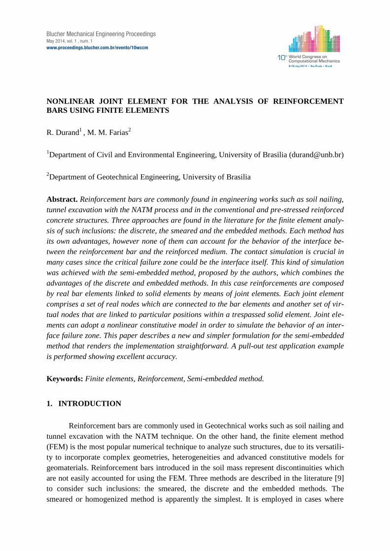
advantage of the embedded method. Figure 1 shows a comparison of the required meshes for

analyses using the discrete and embedded methods. Details of the embedded method may be

found in [5], [8] and [1]. The reinforcement bars are considered by transferring their stiffness

to that of surrounding solid elements. In order to achieve this embedment it is generally as-

sumed a perfect adherence between the bars and the involving solid. This is a serious short-

coming, since failure may happen along the bar-soil interface.

In order to account for the relative displacements in the interface between the bars and

the surrounding medium, [8], [2] and [6] presented an iterative procedure in which the em-

bedded method is used in a first stage and the results are used to solve a second system con-

sidering the bars and joint elements simulated as elasto-plastic springs. The approach works

relatively well, but it still has some drawbacks: for instance, it is not possible to apply external

boundary conditions directly to the bar nodes.

A new method, called semi-embedded, was introduced by Durand (2008) in order to

simulate the interface behavior and to take advantage of the strongest points of the discrete

and embedded methods. In this method, the interface is simulated by means of a set of joint

elements that link the soil with the reinforcements. These joint elements are represented by

non-linear springs located at the nodes of the reinforcement bars and these springs link the

reinforcement with the trespassed elements. Since the springs are attached at specific points,

this approach will be referred to as “punctual interface modeling”.

If the method considers the nodes of the trespassing bars as real nodes that take part in

the global system, then it becomes easy to apply direct boundary conditions, such as pull out

forces or prescribed displacements. This is an additional advantage of the semi-embedded

method in relation to the embedded method in which boundary conditions prescription is

rather cumbersome. In addition, by varying the stiffness of the springs in different regions, it

is also possible to simulate fully anchored zones and free sliding zones, such as in anchored

retaining walls.

The punctual interface approach is still not perfect. The discrete joints do not represent

the behavior along the whole interface, but just at the attachment points to which an arbitrary

proportional area is assigned. Thus, a better approach is desirable in order to take into account

all area along the interface. This paper improves the semi-embedded method providing a new

formulation where the joint elements are not discrete but continuous.

Figure 1. Comparison of finite element meshes for the discrete and embedded element.

2. THE SEMI-EMBEDDED METHOD

An entirely new approach called semi-embedded method, which combines features

from the discrete and the embedded method, was introduced by [3]. As in the embedded

method the reinforcement bars are allowed to trespass the solid elements in any position.

However, the bars elements are discrete and have their own independent nodes, which add

only a few extra degrees of freedom to the background mesh. Although the bars cross the sol-

id elements, these elements are not split into different regions. This is achieved by superim-

posing the bars over the solid elements and connecting them by means of springs which act as

joint elements. The springs connect the independent extra nodes of the bars to fictitious (or

virtual) anchoring nodes along the sides of the solid elements. These virtual nodes do not add

any extra degree of freedom to the system and have their displacements computed by interpo-

lation from the nodes of the solid elements, as if they were perfectly adhered to the soil mass.

The reinforcement bars follow the conventional F.E. formulation, but the interface re-

quires special formulation. Two interface formulations will be described in this paper. The

first one represents the original formulation introduced by [3] called punctual interface model-

ing. The second approach represents a new and more comprehensive formulation which will

be referred to as “continuous interface modeling”.

2.1 Reinforcement discretization

Prior to the analysis with the semi-embedded method, all reinforcements are defined

by their starting and ending points. During the mesh generation process they should be discre-

tized into bar elements within the bounds of the trespassed elements. In addition, joint ele-

ments should be generated in order to link the bar elements with the surrounding soil.

Reinforcement

Finite element

mesh

Conventional finite

element corbel analysis

Reinforcement

Finite element

mesh

Embedded finite

element corbel analysis

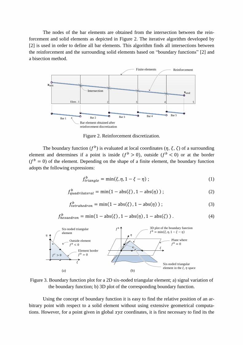
The nodes of the bar elements are obtained from the intersection between the rein-

forcement and solid elements as depicted in Figure 2. The iterative algorithm developed by

[2] is used in order to define all bar elements. This algorithm finds all intersections between

the reinforcement and the surrounding solid elements based on “boundary functions” [2] and

a bisection method.

Figure 2. Reinforcement discretization.

The boundary function ( ) is evaluated at local coordinates ( , , ) of a surrounding

element and determines if a point is inside ( , outside ( ) or at the border

( ) of the element. Depending on the shape of a finite element, the boundary function

adopts the following expressions:

( ; (1)

( ( ( ; (2)

( ( ( ; (3)

( ( ( ( . (4)

Figure 3. Boundary function plot for a 2D six-noded triangular element; a) signal variation of

the boundary function; b) 3D plot of the corresponding boundary function.

Using the concept of boundary function it is easy to find the relative position of an ar-

bitrary point with respect to a solid element without using extensive geometrical computa-

tions. However, for a point given in global coordinates, it is first necessary to find its the

Finite elements

Intersection

Elem . 1 2 3 4 5

Reinforcement

Bar 1 Bar 2 Bar 3 Bar 4 Bar 5

Bar element obtained after

reinforcement discretization

(a) (b)

Element border

Plane whereOutside element

Six-noded triangular

element

Six-noded triangular

element in the , space

3D plot of the boundary function

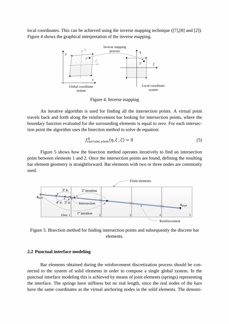
local coordinates. This can be achieved using the inverse mapping technique ([7],[8] and [2]).

Figure 4 shows the graphical interpretation of the inverse mapping.

Figure 4. Inverse mapping

An iterative algorithm is used for finding all the intersection points. A virtual point

travels back and forth along the reinforcement bar looking for intersection points, where the

boundary function evaluated for the surrounding elements is equal to zero. For each intersec-

tion point the algorithm uses the bisection method to solve de equation:

( (5)

Figure 5 shows how the bisection method operates iteratively to find an intersection

point between elements 1 and 2. Once the intersection points are found, defining the resulting

bar element geometry is straightforward. Bar elements with two or three nodes are commonly

used.

Figure 5. Bisection method for finding intersection points and subsequently the discrete bar

elements.

2.2 Punctual interface modeling

Bar elements obtained during the reinforcement discretization process should be con-

nected to the system of solid elements in order to compose a single global system. In the

punctual interface modeling this is achieved by means of joint elements (springs) representing

the interface. The springs have stiffness but no real length, since the real nodes of the bars

have the same coordinates as the virtual anchoring nodes in the solid elements. The denomi-

P

P

Global coordinate

system

Local coordinate

system

Inverse mapping

process

1º iteration

2º iteration3º it.

4º it. 5º it.

Finite elements

Intersection

Elem. 1 2 3 4 5

Reinforcement

nation semi-embedded refers to the springs (not the bars) and comes from the fact that only

one node of the spring is compatible (embedded) with the displacements of the nodes of the

solid element.

Real nodes in the bars have their own equilibrium equations and their displacements

are obtained directly when the global system is solved. However, equilibrium of the fictitious

nodes on the solid elements is satisfied only in a weak sense and their displacements are com-

puted by interpolation for the displacements of the real nodes of the trespassed solid elements.

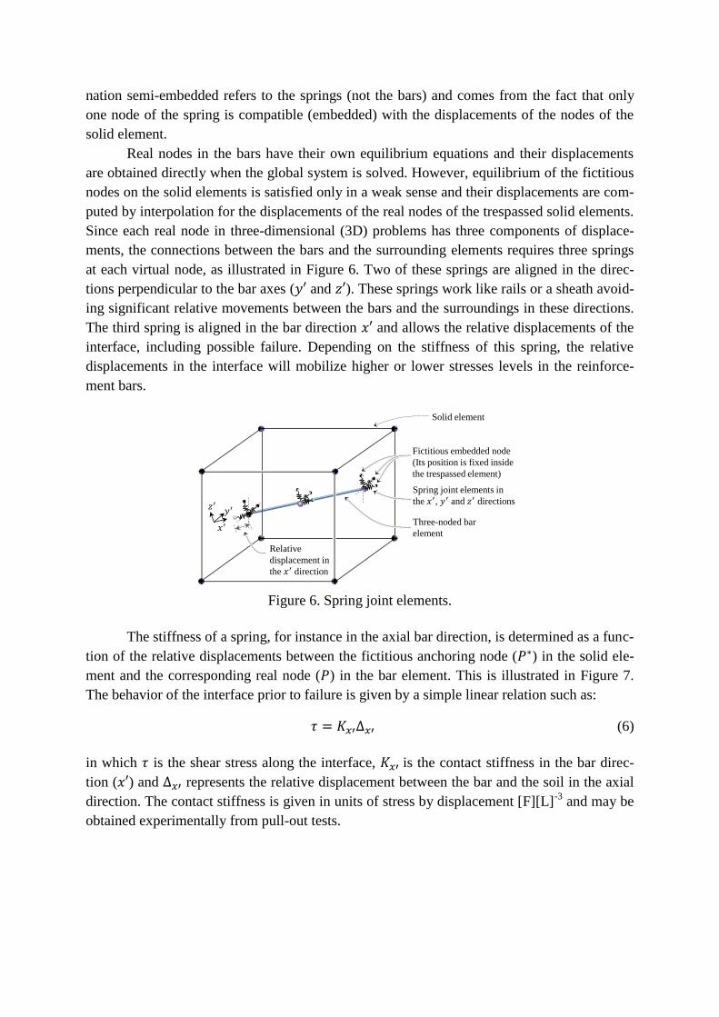
Since each real node in three-dimensional (3D) problems has three components of displace-

ments, the connections between the bars and the surrounding elements requires three springs

at each virtual node, as illustrated in Figure 6. Two of these springs are aligned in the direc-

tions perpendicular to the bar axes ( and ). These springs work like rails or a sheath avoid-

ing significant relative movements between the bars and the surroundings in these directions.

The third spring is aligned in the bar direction and allows the relative displacements of the

interface, including possible failure. Depending on the stiffness of this spring, the relative

displacements in the interface will mobilize higher or lower stresses levels in the reinforce-

ment bars.

Figure 6. Spring joint elements.

The stiffness of a spring, for instance in the axial bar direction, is determined as a func-

tion of the relative displacements between the fictitious anchoring node ( ) in the solid ele-

ment and the corresponding real node ( ) in the bar element. This is illustrated in Figure 7.

The behavior of the interface prior to failure is given by a simple linear relation such as:

(6)

in which is the shear stress along the interface, is the contact stiffness in the bar direc-

tion ( ) and represents the relative displacement between the bar and the soil in the axial

direction. The contact stiffness is given in units of stress by displacement [F][L]-3

and may be

obtained experimentally from pull-out tests.

Three-noded bar

element

Fictitious embedded node

(Its position is fixed inside

the trespassed element)

Solid element

Relative

displacement in

the direction

Spring joint elements in

the , and directions

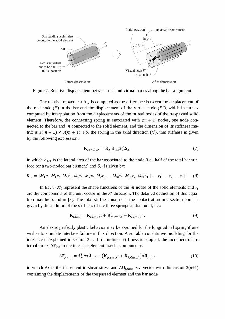
Figure 7. Relative displacement between real and virtual nodes along the bar alignment.

The relative movement is computed as the difference between the displacement of

the real node ( ) in the bar and the displacement of the virtual node ( ), which in turn is

computed by interpolation from the displacements of the real nodes of the trespassed solid

element. Therefore, the connecting spring is associated with ( ) nodes, one node con-

nected to the bar and connected to the solid element, and the dimension of its stiffness ma-

trix is ( ( . For the spring in the axial direction ( ), this stiffness is given

by the following expression:

(7)

in which is the lateral area of the bar associated to the node (i.e., half of the total bar sur-

face for a two-noded bar element) and is given by:

[ ] . (8)

In Eq. 8, represent the shape functions of the nodes of the solid elements and

are the components of the unit vector in the direction. The detailed deduction of this equa-

tion may be found in [3]. The total stiffness matrix in the contact at an intersection point is

given by the addition of the stiffness of the three springs at that point, i.e.:

. (9)

An elastic perfectly plastic behavior may be assumed for the longitudinal spring if one

wishes to simulate interface failure in this direction. A suitable constitutive modeling for the

interface is explained in section 2.4. If a non-linear stiffness is adopted, the increment of in-

ternal forces in the interface element may be computed as:

( ) (10)

in which is the increment in shear stress and is a vector with dimension 3(n+1)

containing the displacements of the trespassed element and the bar node.

Surrounding region that

belongs to the solid element

Bar

Real and virtual

nodes ( and )

initial position

After deformationBefore deformation

Virtual node

Real node

Initial position Relative displacement

2.3 Continuous interface modeling

The continuous interface modeling represents a variant formulation for the interface

element in the semi-embedded method. Whereas the punctual interface modeling considers

joint elements constituted by a set of springs placed at the bar nodes, the continuous interface

modeling replaces the set of springs by a special single joint element. This special element

links a bar element to the corresponding trespassed element without adding extra nodes to the

system. Instead of single contact points, the special joint element represents all the contact

points in the interface and its stiffness is determined by integration using the Gauss quadra-

ture.

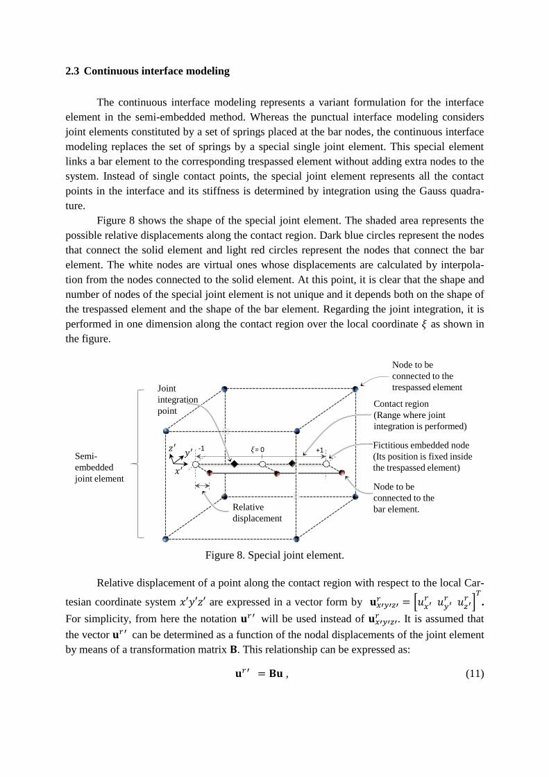
Figure 8 shows the shape of the special joint element. The shaded area represents the

possible relative displacements along the contact region. Dark blue circles represent the nodes

that connect the solid element and light red circles represent the nodes that connect the bar

element. The white nodes are virtual ones whose displacements are calculated by interpola-

tion from the nodes connected to the solid element. At this point, it is clear that the shape and

number of nodes of the special joint element is not unique and it depends both on the shape of

the trespassed element and the shape of the bar element. Regarding the joint integration, it is

performed in one dimension along the contact region over the local coordinate as shown in

the figure.

Figure 8. Special joint element.

Relative displacement of a point along the contact region with respect to the local Car-

tesian coordinate system are expressed in a vector form by [

]

.

For simplicity, from here the notation will be used instead of . It is assumed that

the vector can be determined as a function of the nodal displacements of the joint element

by means of a transformation matrix . This relationship can be expressed as:

, (11)

Node to be

connected to the

bar element.

Fictitious embedded node

(Its position is fixed inside

the trespassed element)

Node to be

connected to the

trespassed element

= 0 +1-1Semi-

embedded

joint element

Contact region

(Range where joint

integration is performed)

Relative

displacement

Joint

integration

point

where the joint displacements vector comprises all displacements of the nodes of the

trespassed element plus the displacements of the nodes of the bar element according to:

[

] . (12)

Once matrix is calculated, the joint element stiffness matrix can be determined in a

traditional way as:

∫ , (13)

where

represents the constitutive matrix of the joint material that relates the relative dis-

placements vector with the increments in the contact stress vector

[ ] and is the area of the cylindrical contact surface. Using the Gauss

quadrature and since , where is the perimeter of the contact section, the stiffness

matrix can be expressed as the summation along the integration points:

∑

. (14)

The matrix is fundamental in this formulation and its determination will be outlined

now. First, it is considered that the displacement vector at the virtual embedded nodes are

obtained as a function of the nodal displacements of the trespassed element. This relation-

ship can be determined by interpolation using the shape functions of the solid element. In

this case means the shape function of solid element node evaluated at the embedded

node . Assuming a solid element with nodes and embedded nodes in the joint element

then:

{

}

[

]

{

}

(15)

The Eq. 15 can be expressed in a condensed matrix form as:

. (16)

Assuming a preliminary joint displacement vector of the form [ ] , the relative dis-

placement vector in the system evaluated at an arbitrary point along the contact region

can be expressed by interpolation as:

[ ] {

} , (17)

where is a matrix containing the direction cosines in the directions of , and

and is a matrix that contains interpolation functions for the contact region which are as-

sumed to be equal to those of the bar element. The matrix can be represented in extended

form as:

[

]. (18)

Substituting Eq. 15 into Eq. 17, the following expression is obtained:

[ ] [

] , (19)

which after some rearrangement can be expressed by convenience as:

[ ] [

] (20)

With Eq. 20, a direct relationship between the relative displacements vector and the

joint displacement vector [ ] is obtained by means of the product [ ]

which by comparison with the Eq. 11 represents the desired matrix . Later, the internal forc-

es in the joint element can be calculated simply as:

∫ , (21)

or using the Gauss quadrature, as the summation along the integration points:

∑

. (22)

Two Gauss integration points are recommended for the case of two embedded nodes, and

three for the case of three embedded nodes.

2.4 Interface constitutive modeling

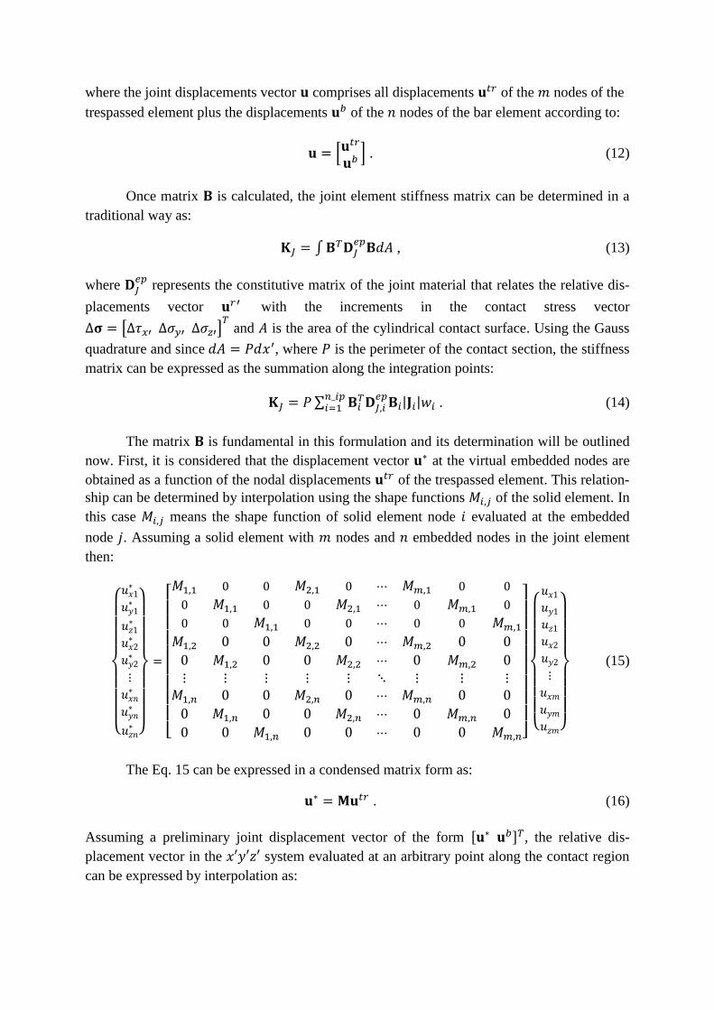
For a given point in the interface this constitutive modeling aims to find the elasto-

plastic relationship between the relative displacements vector [

]

(see

Figure 9) and the corresponding stress vector in the interface given by [ ] .

Assuming that the interface failure occurs only along the bar direction , the elasto-plastic

modeling will just relate with . These variables will be denoted simply as and for

the sake of simplicity. For the other variables, assuming an elastic relationship with high stiff-

ness should be enough, since it is considered that relative displacements in the directions

and are negligible.

Figure 9. Directions of displacement vector components , and .

This derivation will consider a one dimensional elasto-plastic model with some little

hardening, similar to a scheme proposed by [10]. In this case, the relative displacement

plays the role of deformation in the conventional elastic-plastic theory. The interface strength

may be given by a criterion similar to that of Mohr-Coulomb (MC), by assuming an adhesion

parameter and a friction angle . In this case, the MC failure criterion for the interface can

be expressed as:

, (23)

where is the shear stress in the contact region in the bar direction and represents the

average confining stress which can be obtained by interpolating the trespassed element stress-

es as described in section 2.5.

Before failure, a simple elastic behavior can be adopted by means of an interface shear

stiffness modulus :

. (24)

The stiffness modulus can be obtained experimentally from pull-out tests according to:

, (25)

where and are, respectively, the pull-out force and the final displacement obtained

during the test.

Regarding the confining stress in Eq. 23, it is worth noting that this value is not a

constant and depends on the surrounding stresses level that can change during the analysis.

Figure 10 shows two stress-displacement trajectories and which are limited by the MC

failure criterion. Both trajectories have different confining stress values, so they will reach the

failure surface at different points.

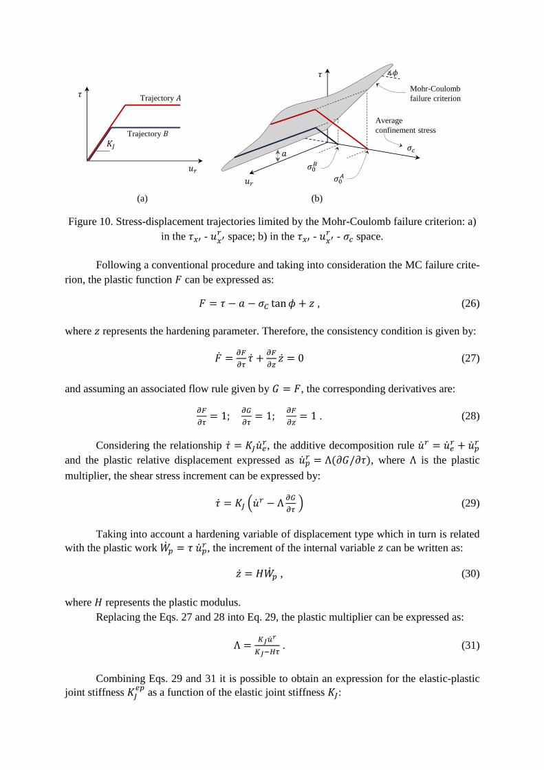
Figure 10. Stress-displacement trajectories limited by the Mohr-Coulomb failure criterion: a)

in the - space; b) in the -

- space.

Following a conventional procedure and taking into consideration the MC failure crite-

rion, the plastic function can be expressed as:

, (26)

where represents the hardening parameter. Therefore, the consistency condition is given by:

(27)

and assuming an associated flow rule given by , the corresponding derivatives are:

. (28)

Considering the relationship , the additive decomposition rule

and the plastic relative displacement expressed as ( , where is the plastic

multiplier, the shear stress increment can be expressed by:

(

) (29)

Taking into account a hardening variable of displacement type which in turn is related

with the plastic work , the increment of the internal variable can be written as:

, (30)

where represents the plastic modulus.

Replacing the Eqs. 27 and 28 into Eq. 29, the plastic multiplier can be expressed as:

. (31)

Combining Eqs. 29 and 31 it is possible to obtain an expression for the elastic-plastic

joint stiffness

as a function of the elastic joint stiffness :

Mohr-Coulomb

failure criterion

Average

confinement stress

(a) (b)

Trajectory

Trajectory

. (32)

In addition, the increment in the hardening parameter is given by:

(33)

Since the vector of relative displacements contains components in the three direc-

tions, it is convenient to express an elasto-plastic matrix that relates the increment in relative

displacements with the joint stress increment:

[

] [

] [

] , (34)

where represent the stiffness in the directions and perpendicular to the interface. Fi-

nally, the elastic-plastic matrix for the semi-embedded joint element can be written simply as:

[

] . (35)

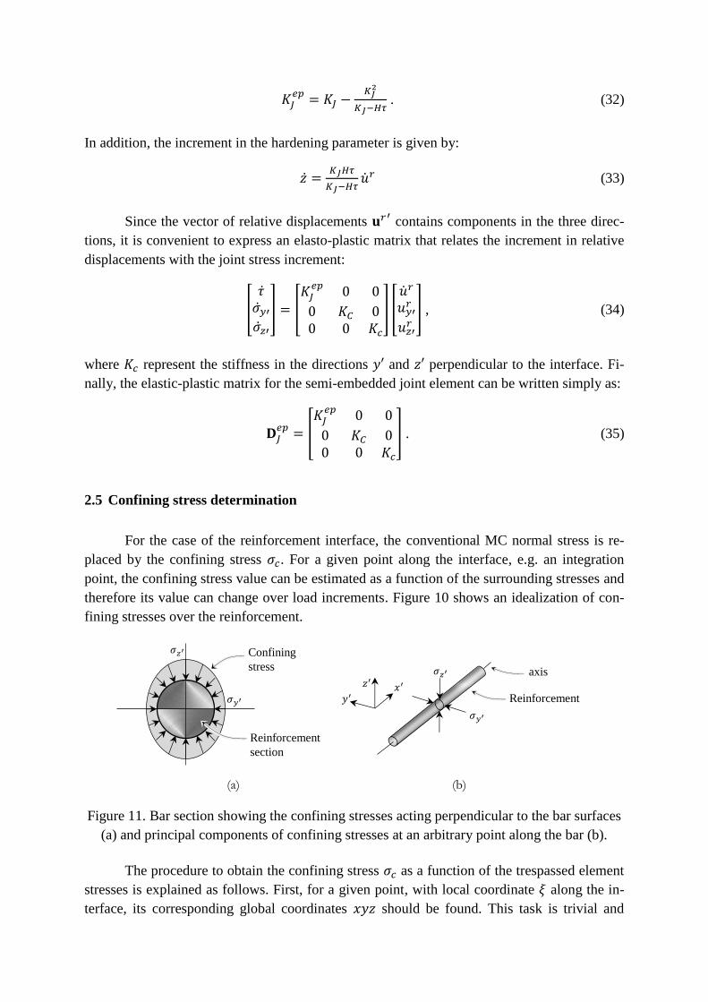
2.5 Confining stress determination

For the case of the reinforcement interface, the conventional MC normal stress is re-

placed by the confining stress . For a given point along the interface, e.g. an integration

point, the confining stress value can be estimated as a function of the surrounding stresses and

therefore its value can change over load increments. Figure 10 shows an idealization of con-

fining stresses over the reinforcement.

Figure 11. Bar section showing the confining stresses acting perpendicular to the bar surfaces

(a) and principal components of confining stresses at an arbitrary point along the bar (b).

The procedure to obtain the confining stress as a function of the trespassed element

stresses is explained as follows. First, for a given point, with local coordinate along the in-

terface, its corresponding global coordinates should be found. This task is trivial and

(a) (b)

Reinforcement

section

Confining

stress

Reinforcement

axis

easily done by interpolation of the embedded nodal coordinates. After the global coordinates

of the point are found, they should be converted to local coordinates related to the tres-

passed element. For these coordinates, the stress vector could be found by a process of

extrapolation and interpolation from the stresses in the trespassed element according to:

( ( ) , (36)

where is a matrix containing the stresses from all integration points of the trespassed ele-

ment:

[

]

, (37)

E is an extrapolation matrix that allows the determination of nodal values from the values

given at integration points (see [4]). is a vector containing the trespassed element shape

functions evaluated at local coordinates and .

The stresses vector given by Eq. 36 can be transformed into the system by a

conventional change in coordinates systems by means of a matrix according to:

{

}

[

]

{

}

, (38)

where , and are scalars representing the directional cosines between the and

coordinate systems. Applying this coordinates transformation in Eq. 36 the following expres-

sion is obtained:

( ( ) (39)

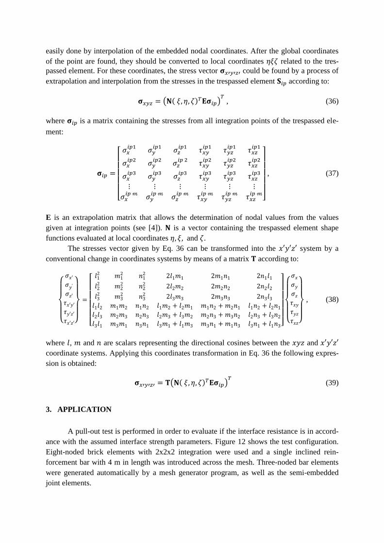
3. APPLICATION

A pull-out test is performed in order to evaluate if the interface resistance is in accord-

ance with the assumed interface strength parameters. Figure 12 shows the test configuration.

Eight-noded brick elements with 2x2x2 integration were used and a single inclined rein-

forcement bar with 4 m in length was introduced across the mesh. Three-noded bar elements

were generated automatically by a mesh generator program, as well as the semi-embedded

joint elements.

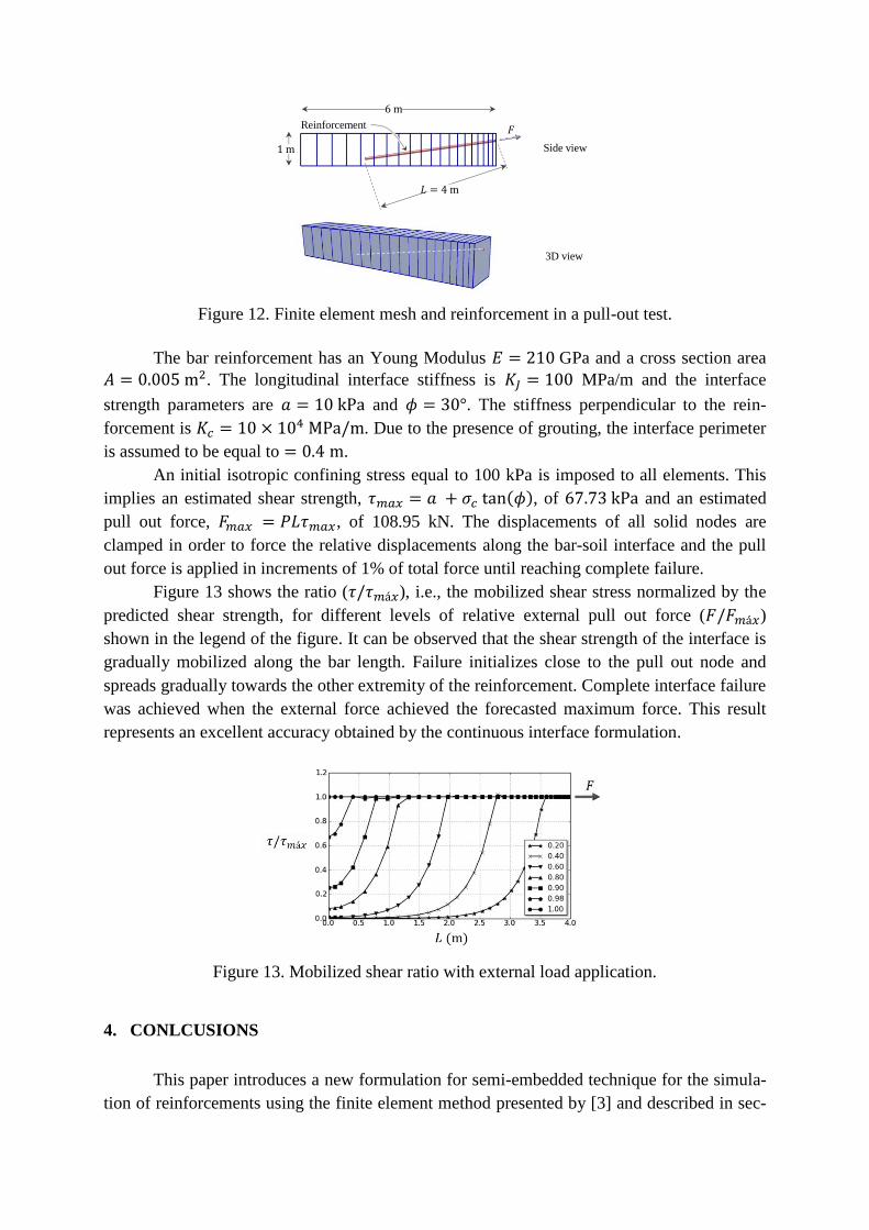
Figure 12. Finite element mesh and reinforcement in a pull-out test.

The bar reinforcement has an Young Modulus GPa and a cross section area

. The longitudinal interface stiffness is MPa/m and the interface

strength parameters are and . The stiffness perpendicular to the rein-

forcement is . Due to the presence of grouting, the interface perimeter

is assumed to be equal to .

An initial isotropic confining stress equal to 100 kPa is imposed to all elements. This

implies an estimated shear strength, ( , of and an estimated

pull out force, , of 108.95 kN. The displacements of all solid nodes are

clamped in order to force the relative displacements along the bar-soil interface and the pull

out force is applied in increments of 1% of total force until reaching complete failure.

Figure 13 shows the ratio ( ), i.e., the mobilized shear stress normalized by the

predicted shear strength, for different levels of relative external pull out force ( )

shown in the legend of the figure. It can be observed that the shear strength of the interface is

gradually mobilized along the bar length. Failure initializes close to the pull out node and

spreads gradually towards the other extremity of the reinforcement. Complete interface failure

was achieved when the external force achieved the forecasted maximum force. This result

represents an excellent accuracy obtained by the continuous interface formulation.

Figure 13. Mobilized shear ratio with external load application.

4. CONLCUSIONS

This paper introduces a new formulation for semi-embedded technique for the simula-

tion of reinforcements using the finite element method presented by [3] and described in sec-

Side view

Reinforcement

3D view

tion 2.2. The main advantage of this new formulation is that the interface between a bar and

the reinforced medium can be simulated as a continuum using a single special interface ele-

ment instead of a set of springs.

In addition to the neater formulation, the proposed changes make implementation and

further development much simpler and straightforward.

The method can be applied in 2D or 3D and it is independent on the element type or

constitutive behavior of the solid background elements. In this paper, it was tested for a sim-

ple pull-out test with excellent accuracy.

5. REFERENCES

[1] Andrade, H.A.C., “Numerical procedures for the analisys of drainage elements is soils”.

MSc Dissertation, Pontifical Catholic University of Rio de Janeiro, Rio de Janeiro, Brazil,

125 p, 2003.

[2] Durand, R., “Embedded stiffness method in the tree-dimensional analysis of reinforce-

ments via finite elements”. MSc Dissertation, University of Brasilia, Brasilia, Brazil, 95

p., 2003.

[3] Durand, R., “Three-dimensional analysis of geotechnical structures subjected to rein-

forcement and drainage”. PhD Thesis, University of Brasilia, Brasilia, Brazil, 153 p, 2008.

[4] Durand, R., Farias, M.M., “A generalized method for the extrapolation of internal values

to the nodal points of finite elements”. In: 2nd International Workshop in Computational

Geotechnics, IWS-Fortaleza, 1, 21-28, 2004.

[5] Elwi, A.E., Hrudey, T.M., “Finite element model for curved embedded reinforcements”.

Engineering Mechanics, ASCE, 115(4), 740-754, 1989.

[6] Farias, M. M., Durand, R., “Embedded stiffness approach to compute the optimum con-

figuration of reinforcements”. In: NUMOG IX, International Symposium on Numerical

Models in Geomechanics, 1, 549-555, 2004.

[7] Farias, M.M., Naylor, D.J., “Safety analysis using finite elements”. Computers and Ge-

otechnics, Elsevier Science, 22(2), 165-181, 1998.

[8] Hartl, H., “Development of a continuum-mechanics-based tool for 3D finite element anal-

ysis of reinforced concrete structures and application to problems of soil-structure interac-

tion”, PhD Thesis, Graz University of Technology, Graz, Austria, 250 p, 2002.

[9] Kwak, H.G., Filippou, F.C., “Finite element analysis of reinforced concrete structures

under monotonic loads”. Report No. UCB/SEMM-90/14, Department of Civil Engineer-

ing, University of California, Berkeley, USA, 120 p, 1990.

[10] Nakai, T., “Finite element computations for active and passive earth pressure problems

of retaining wall”. Soils and Foundations, 25(3), 98-11, 1985.