-1-

NONLINEAR FOURIER ANALYSIS OF DEEP-WATER, RANDOM WAVE TRAINS

A. R. Osborne, M. Onorato and M. Serio

Dipartimento di Fisica Generale dell'Università Via Pietro Giuria 1, Torino 10125, Italy

Donald T. Resio

U. S. Army Engineer Research and Development Center

Coastal and Hydraulics Laboratory, 3909 Halls Ferry Road Vicksburg, MS 39180-6199, U.S.A.

1. INTRODUCTION The focus of this paper is to address a new approach for the Fourier analysis of deep-water wave trains. The method is intrinsically nonlinear and describes a nonlinear Fourier spectrum which includes (1) The nonlinear superposition of quasi-linear sine

or Stokes wave components. (2) The nonlinear superposition of nonlinear wave

packets and their space/time dynamics. (3) The Stokes wave nonlinearity. (4) The influence of the wave/current interaction on

the nonlinear spectrum. How is it that a nonlinear Fourier approach can simultaneously contain all of these features? One begins by writing a linear wave equation for the envelope of a linear wave train:

i(ψ t + Cgψ x ) + µψ xx = 0 (1)

where ψ (x,t ) is the complex envelope of the wave train, Cg is the group speed, ωo is the carrier frequency, ko is the wave number, ωo

2 = gko is the deep-water dispersion relation and µ = −ω o / 8ko

2 . This is just about the simplest wave equation imaginable. The complex envelope, ψ (x,t ), is related to the surface elevation, η(x,t ), by:

η(x,t ) = ψ (x,t )eiko x −iω ot + c.c. (2)

Because (1) and (2) are linear equations the Fourier structure is trivial: The usual linear Fourier transform solves (1) for all (Cauchy) initial conditions! So, assuming that (1) is true, then (a) modeling of wave trains is simple (the FFT algorithm suffices for computing the space/time evolution), (b) the Fourier analysis of oceanic data is also straightforward using the FFT and (c) filtering, computation of transfer functions and the computation of power spectra follows in a natural way. How can we ever imagine doing anything better? We have all the tools for understanding how linear waves behave in the oceanic environment. Of course (1) is narrow banded, but we can always improve this feature to arbitrary

order by adding additional linear dispersive terms to the equation.

For wind-wave modeling we ordinarily go a step farther by introducing a kinetic equation which includes nonlinear three, four or five-wave interactions and the results have resulted in spectacular improvement in predictive capability over the last few decades. However wind wave models, being based on kinetic equations, filter out coherent effects in a nonlinear wave train, i.e. solitary waves, soliton packets and unstable packet modes (in the Benjamin-Feir sense) tend to be thrown out like the baby in the bath water, to use traditional idiom. Indeed a major contribution to oceanic rogue wave dynamics (extreme waves) has been recently attributed to the Benjamin-Feir instability by a number of authors (Osborne, et al [2000]; Trulsen and Dysthe [1997; 1999], Janssen [2003]). Is it possible to do something really simple to modify (1) to give us back some of these nonlinear effects lost in the conversion to kinetic equations? Can it be that a kind of nonlinear Fourier analysis awaits discovery while proceeding in this direction? Can it be that this nonlinear Fourier analysis can also solve kinetic equations? The answers to these and many other fundamental questions are in the affirmative. A step in this direction is documented herein.

Indeed we are about to describe and use a method which allows one to implement a kind of nonlinear Fourier analysis procedure which has two kinds of nonlinear Fourier modes: (1) weakly nonlinear Stokes waves and (2) nonlinear, unstable wave packets which have complex dynamics. The unstable wave packets can, in certain circumstances, lead to extreme waves that can be interpreted as rogue or freak waves.

To modify (1) for nonlinear effects we have carried out the simplest possible approach. We have added a simple cubic nonlinearity:

i(ψ t + Cgψ x ) + µψ xx + ν ψ 2ψ = 0 (3)

-2-

where ν = −ω oko2 / 2 . This is the so-called nonlinear

Schroedinger (NLS) equation, the simplest possible nonlinear wave equation for deep-water wave dynamics. We realize that this is just a small step toward full understanding of nonlinear wave trains, but it is an important step, because as we shall see there is much to learn. Eq. (3) has the list of surprising properties given in the first paragraph above. These properties arise as a consequence of the exact solution of (3) for periodic boundary conditions using the inverse scattering transform. In the last half of the twentieth century a number of important theoretical developments have been made with regard to the understanding of nonlinear wave propagation [Novikov, et al, 1980; Ablowitz and Segur, 1981; Dodd, et al, 1982; Newell, 1985]. Of particular relevance to the present work has been the discovery of large classes of nonlinear wave equations whose solutions may be computed without approximation using a new technique referred to as the inverse scattering transform (IST). IST may be viewed as a kind of nonlinear Fourier analysis, valid for fully nonlinear wave motion, which has many of the nice features that render ordinary Fourier analysis such a useful tool for the analysis of oceanic wave motions. Practical implementation of IST has been made possible by a number of theoretical advances [Boyd, 1981, 1990; Date and Tanaka, 1976; Dubrovin, et al., 1976; Flaschka and McLaughlin, 1976; Its and Matveev, 1975; McKean and Trubowitz, 1976] with regard to the case for periodic boundary conditions and in a recent papers of Osborne [1995, 2002] in which techniques are developed for the simple exploitation of the method from physical, mathematical and numerical points of view. The approach has been cast in terms of a kind of nonlinear Fourier analysis which, in the small amplitude limit, reduces to the ordinary, linear Fourier transform. It is for this reason that the nonlinear Fourier approach may be viewed as a generalization of linear Fourier analysis. The remainder of the paper is organized as follows. Section 2 discusses linear Fourier analysis while Section 3 discusses nonlinear Fourier analysis for the NLS equation. Section 4 gives three examples of unstable wave packets. Section 5 discusses modulation theory for the NLS equation and provides a basis for a nonlinearity (Benjamin-Feir) parameter based on inverse scattering theory. Characteristics of random wave trains subjected to the BF instability are briefly reviewed in Section 6. Section 7 discusses application of periodic inverse scattering theory to the analysis of random waves in the wave tank facility at Marintek, Trondheim, Norway. 2. LINEAR FOURIER ANALYSIS

Fourier analysis allows the construction of linear wave trains, η(x ,t ) , by a linear superposition of sine waves:

η(x,t ) = Cn cos knx − ω nt + φn( )n=1

N

∑ (4) In the present case there are N sine waves which are interpreted as "degrees of freedom" or "Fourier components" in the wave train. In Eq. (4) the Cn are the Fourier amplitudes, the kn are the wave numbers, the ω n are the frequencies and the φn are the phases. The relationship between the frequencies, ω n , and the wave numbers, kn , is given by the dispersion relation, written symbolically: ω n = ωn (kn ). The dispersion relation defines the physics via the correspondences

∂∂t

↔ −iω , ∂

∂x↔ ik

For example the simple dispersion relation for deep water wave trains is given by

ω = Cgk + µk 2 (5) which has the associated partial differential equation (1). The simplest periodic solution to (1) is a travelling sine wave η(x,t ) = Co cos ko x − ωot + φo( ) from which the general Fourier solution for N components may be constructed by (4). The important point is that the amplitudes of the sine waves and their phases are constants of the motion, provided that the motion is linear. In oceanic applications one is often interested in the analysis of time series, i.e. measurements of the wave amplitude, η(0, t) , taken at a fixed spatial location over some convenient time interval; this implies setting x = 0 in (4).

3. NONLINEAR FOURIER ANALYSIS We proceed by writing the NLS equation in a form that is simpler for theoretical calculations

iut + uxx + 2 u2 u = 0 (6) This equation arises from (3) by a simple rescaling and translation:

u = λψ ; µt → t ; x − Cgt → x (7) The Fourier structure of the nonlinear Schroedinger equation (6) is given by [Kotljarov and Its, 1976; Tracy and Chen, 1988]

u(x, t) = Aoθ(x, t | B,δ − )θ(x, t | B,δ + )

e2 iAo2t (8)

where the Riemann theta functions, θ(x, t | B,δ± ), are given by:

-3-

θ(x, t) = ...M2 = −∞

∞

∑M1 = −∞

∞

∑ (9)

... exp i Mn Xnn=1

N

∑ +12

Mmn=1

N

∑ Bmn Mnm =1

N

∑

MN =−∞

∞

∑

where Xn = kn x − ωnt − δ n

± The wave numbers, kn , frequencies, ωn , and phases, δ n , are computed by the methods of algebraic geometry (see [Osborne, 2002] for a review and a list of references). It should be noted that the theta functions (9) are just generalized Fourier series, where the spectral amplitudes correspond to a (Riemann) matrix, B , rather than to a vector, Cn , as in linear Fourier analysis (4). To better understand the solutions of (3) using the nonlinear Fourier decomposition (9) let us consider a number of simple examples. The ratio of theta functions, θ(x, t | B,δ − ) / θ(x, t | B,δ + ) , is the complex modulation envelope function. When there is no modulation, θ(x, t | B,δ − ) / θ(x, t | B,δ + ) = 1, we have

u(x, t) = Aoe2 iAo2t (10)

This is the so-called plane wave solution of the NLS equation. It corresponds to an unmodulated carrier wave. To understand these nonlinear spectral solutions it is necessary to discuss the so-called spectral eigenvalue problem for the NLS equation, first found by Zakharov and Shabat [1972]: iφ1x + iuφ2 = λφ1

(11) −iφ2 x + iu*φ1 = λφ2 The values of the eigenvalues are crucial for describing the solutions (8) of NLS (6). Here we assume periodic boundary conditions to determine solutions of (11). Indeed one works in the λ -plane, Fig. 1.

Figure. 1. Lambda plane where the nonlinear Fourier spectrum for the NLS equation lives. The lambda plane is a complex plane for the eigenvalues of (11) which have real and imaginary parts, λ = λR + iλI , corresponding to the real and imaginary axes in Fig. 1. The simplest case is for the plane wave solution (10). This is the case of an unmodulated carrier wave of amplitude Ao . In the lambda plane (for which the spectrum is a perfect mirror image between the upper and lower half planes) the eigenvalues λ = ±iAo on the imaginary axis correspond to the carrier wave, Ao . The modulations correspond to double points (pairs of eigenvalues) connected by spines (curves of spectrum connecting the double points). Two kinds of spectrum exist for NLS: (1) Stokes waves (for which the two eigenvalues of the double point are connected by a spine across the real axis) and (2) unstable wave packets (for which the two eigenvalues are connected by a spine contained entirely in the upper half plane (and also in the lower half plane by specular reflection). The Stokes waves have a Riemann matrix which is 1x1 (a scalar) while the unstable wave packets have a 2x2 matrix. Unstable wave packets are characterized by double points in the upper and lower half planes. Their spectrum contains five numbers: Ao, ε,θ, λRc , λIc (see Fig. 1). Here Ao is the carrier amplitude, ε is the half-distance between the double points, θ is the angle of a straight line connecting the double points and the complex pair (λRc, λIc ) corresponds to the centroid of the double points in the lambda plane. Thus five parameters are required to describe a single unstable wave packet, i.e. the nonlinear interaction between the carrier and a long-wave unstable modulation. The unstable packet modes have very interesting physical behavior: They are packets which can, early in their evolution, correspond to a small modulation of the carrier and

-4-

then later become large modulations which can reach up to several times the carrier amplitude. An important property of an unstable packet mode is the maximum amplitude it can reach during its evolution. This can be computed by the simple formula:

ηmaxAo

= 2λIAo

+ 1 (12)

In the light of this discussion of the lambda plane it is interesting to recall where historical wave tank experiments have resided in the lambda plane. Roughly, these correspond to the small vertical box of eigenvalue pairs on or near the imaginary axis as shown in Fig. 1; these correspond to three of the five parameters being identically zero: Ao, 0,0, 0, λIc. Indeed, based on this observation, most of the lambda plane has yet to be explored. In our view, many surprises await future exploration of the entire plane. We already know about Stokes wave solutions of the NLS equation, i.e. they correspond to the dnoidal wave solutions of the equation and are double points with spines crossing the real axis (Fig. 1). To save space we move immediately to solutions of NLS that correspond to unstable wave packets. 4. ANALYTICAL EXAMPLES OF UNSTABLE WAVE PACKETS A large number of examples of unstable wave packets are known [Osborne, et al, 2000]. We consider three cases: (1) Ao, 0,0, 0, Ao / 2 , (2) Ao, 0,0, 0, Ao and (3) Ao, 0,0, 0, 2Ao . The first case lies on the imaginary axis below the carrier, the second lies directly on the carrier and the third lies above the carrier in the lambda plane. The first case considered has the following solution to the NLS equation:

u(x, t) = Aocos[ 2 Ao x]sech[2Ao

2t] + i 2tanh[2Ao2t]

2 − cos[ 2Aox]sech[2Ao2t]

e

2iAo2t

(13) The imaginary part of the eigenvalue is λI = iAo / 2 and the maximum packet amplitude is then given by

ηmaxAo

= 2λIAo

+ 1 ≅ 2.4

Figure. 2. Modulus of unstable wave packet that lies below the carrier in the complex lambda plane with spectrum: Ao, 0,0, 0, Ao / 2 . This case is typical of previous studies of the Benjamin-Feir instability, i.e. we have a small amplitude modulation in the far past. As seen in Fig. 2 the small modulation is not easily visible at early times, it appears to be a broad flat plane over all x at small t. Then exponential growth is seen to lead to a finite amplitude of ~2.41 times the carrier amplitude and then the wave decreases in amplitude as the modulation effectively disappears for large times. This solution to NLS (13) is periodic in x and decays exponentially for large past and future times; it can be viewed as a single nonlinear mode (a single Fourier component) of NLS with a 2x2 period matrix. The second case (which lies directly on the carrier) is shown in Fig. 3. It has the exact solution (see [Osborne, et al 2000] and references therein]) given by

u(x, t) = Ao 1−4(1+ 4iAo

2t )1 +16Ao

4t2 + 4Ao2 x2

(14)

Here the imaginary part of the eigenvalue is λI = iAo and thus the maximum wave height is given by:

ηmaxAo

= 2λIAo

+ 1 = 3.0

From (14) we see that this solution to NLS is characterized by an algebraic decay for large x and t. In the spirit of the periodic inverse scattering transform (14) is a nonlinear Fourier component in the theory.

-5-

Figure. 3. Modulus of unstable wave packet that lies on the carrier in the complex lambda plane with spectrum: Ao, 0,0, 0, Ao. The third case (above the carrier) is shown in Fig. 4.

u(x, t) = Ao 1+2 cos[4 2Ao

2t] + i 2 sin[4 2Ao2t]( )

cos[4 2 Ao2t] + 2 cosh[2Ao x]

e2 iAo

2t

(15) The eigenvalue is given by λI = i 2Ao so that the maximum height has the value

ηmaxA

= 2λ IA

+ 1 ≅ 3.8 This case lies above the carrier and is no longer a small amplitude modulation for times far in the past. Indeed the solution is periodic in t and exponentially decaying in x. Note that for small time in Fig. 4 the spatial variation in the solution is a large amplitude modulation. This behavior is characteristic of spectral components with centroid above the carrier in the lambda plane [Tracy and Chen, 1988].

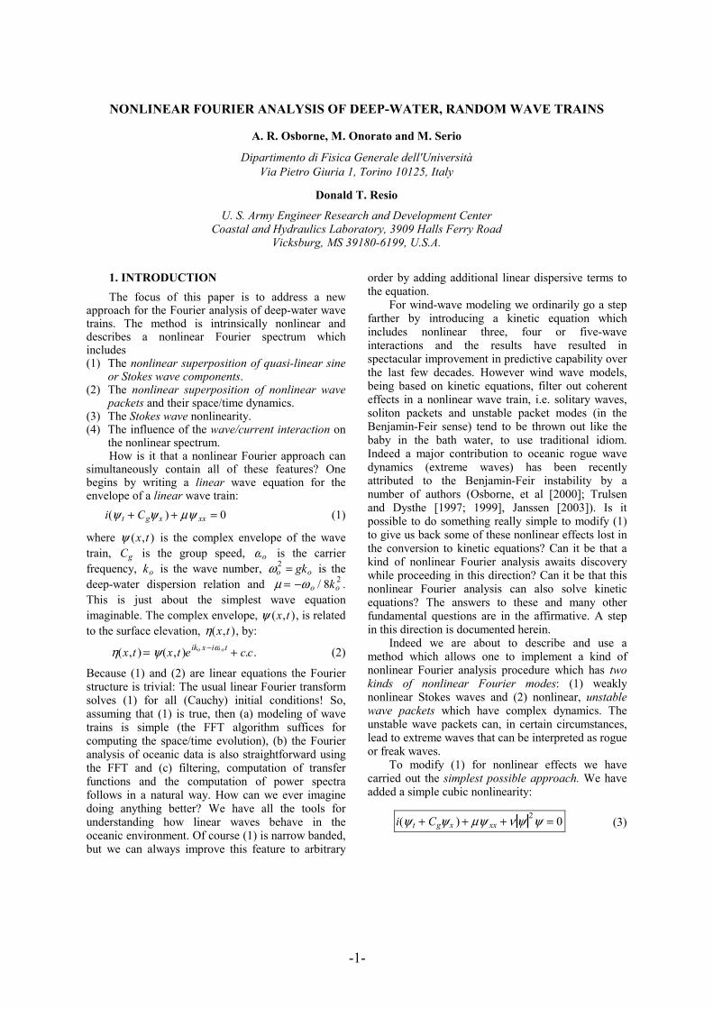
Figure. 4. Modulus of unstable wave packet that lies above the carrier in the complex lambda plane with spectrum: Ao, 0,0, 0, 2Ao . At this points is seems clear that there are an infinite number of solutions of the NLS equation each corresponding to particular values for the parameters in the spectrum Ao, ε,θ, λRc , λIc . This is also true of the linear Fourier spectrum where there is a four-parameter family for amplitude A, wave number k, frequency ω and phase φ for each sine wave component: A, k, ω, φ . However, for the IST solution of the NLS equation the basis functions and the space/time dynamics are much less boring than simple sine waves, as verified by Figs. 2-4. 5. MODULATION THEORY FOR THE NLS EQUATION Small amplitude modulation theory for the NLS equation predicts a number of interesting features about the nonlinear propagation of initially small amplitude sine wave modulations. One of the most important is shown in Fig. 5 where a small amplitude modulation of a carrier wave is shown (both the real and the imaginary parts of the carrier are given). At a later time this small modulation develops into an unstable wave packet as seen in Fig. 6. In the present case the maximum amplitude is about 2.6 times the carrier height. One of the important properties of an unstable wave packet is the growth rate:

Ω = iωoko2ao

2 K2 2ko

2ao

1− K

2 2ko2ao

2

(16)

This is Yuen’s result [Yuen, 1988] when squared, but we leave this equation in the above form to emphasize the dependence on the Benjamin-Feir parameter. The

-6-

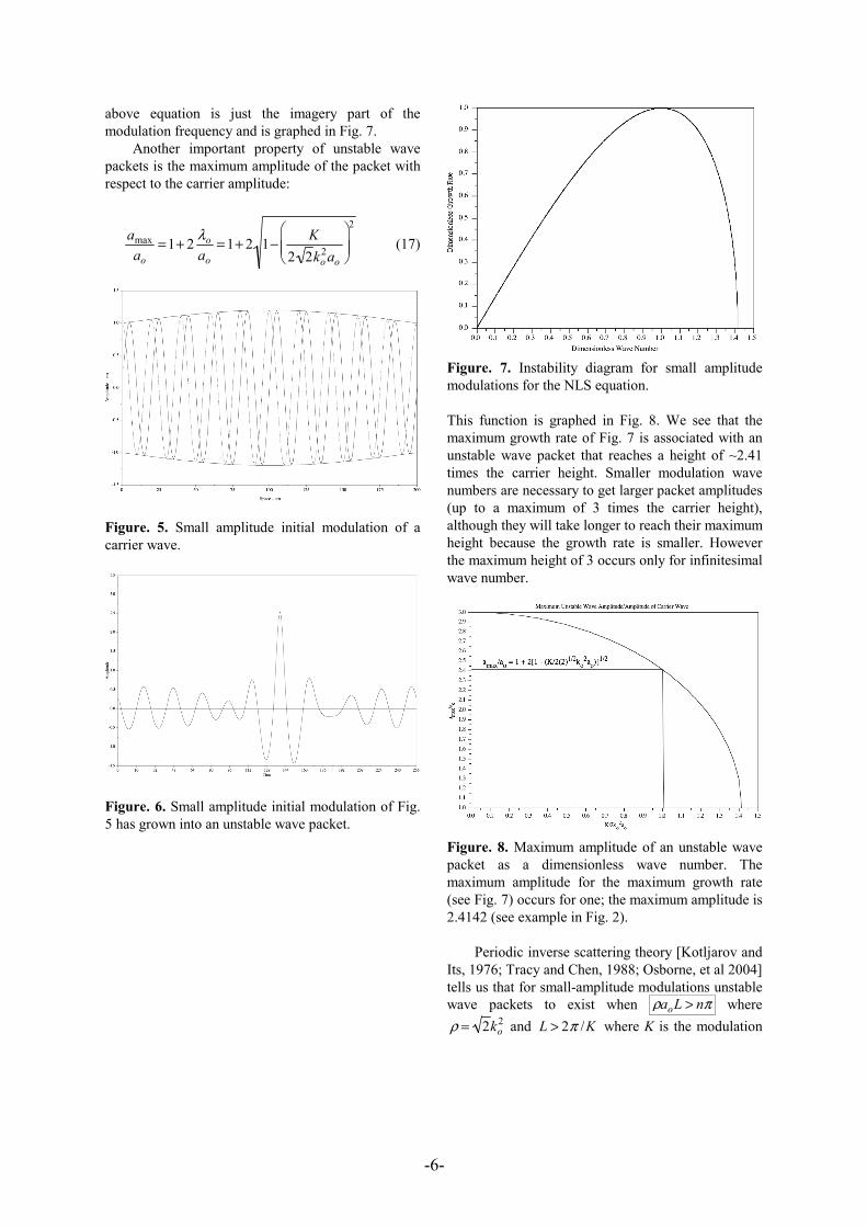
above equation is just the imagery part of the modulation frequency and is graphed in Fig. 7. Another important property of unstable wave packets is the maximum amplitude of the packet with respect to the carrier amplitude:

amax

ao=1+ 2 λo

ao= 1+ 2 1− K

2 2ko2ao

2

(17)

Figure. 5. Small amplitude initial modulation of a carrier wave.

Figure. 6. Small amplitude initial modulation of Fig. 5 has grown into an unstable wave packet.

Figure. 7. Instability diagram for small amplitude modulations for the NLS equation. This function is graphed in Fig. 8. We see that the maximum growth rate of Fig. 7 is associated with an unstable wave packet that reaches a height of ~2.41 times the carrier height. Smaller modulation wave numbers are necessary to get larger packet amplitudes (up to a maximum of 3 times the carrier height), although they will take longer to reach their maximum height because the growth rate is smaller. However the maximum height of 3 occurs only for infinitesimal wave number.

Figure. 8. Maximum amplitude of an unstable wave packet as a dimensionless wave number. The maximum amplitude for the maximum growth rate (see Fig. 7) occurs for one; the maximum amplitude is 2.4142 (see example in Fig. 2). Periodic inverse scattering theory [Kotljarov and Its, 1976; Tracy and Chen, 1988; Osborne, et al 2004] tells us that for small-amplitude modulations unstable wave packets to exist when ρaoL > nπ where ρ = 2ko

2 and L > 2π /K where K is the modulation

-7-

wave number, ao is the carrier amplitude and ko is the carrier wave number. Here n is an integer, n =1,2... that counts the number of unstable wave packets in a wave train. This provides a useful definition of nonlinearity in terms of a kind of Benjamin-Feir parameter:

IBF = ρaoLπ

= 2 2ko2ao

K> n (18)

We see that this is the same parameter that appears in the growth rate (16) and the maximum amplitude (17) of an unstable packet, which we now rewrite:

Ω = iωoko2ao

2 IBF2 −1IBF

2 (19)

amax

ao=1+ 2

IBF2 −1IBF

(20)

Two of the most useful results for estimating unstable wave packet behavior can be written in terms of the Benjamin-Feir parameter! It is also clear that unstable wave packet (a nonlinear mode in the spectrum) has the imaginary part of the centroid of the associated double point that is also a function of the Benjamin-Feir parameter:

λI = aoIBF

2 − 1IBF

and the inverse:

IBF =ao

ao2 − λI

2

Thus there is a unique relationship between the BF parameter and the spectrum of an unstable wave packet. 6. CHARACTERISTICS OF RANDOM WAVE TRAINS USING IST Here we focus on a time series of length T, significant wave height Hs = 4σ (σ is the standard deviation of the time series) and fo is the peak spectral frequency. Use the fact that ∆k /ko = 2∆f / fo (where ∆f =1/T , ∆k ≡ K ) and the Benjamin-Feir parameter becomes:

IBF = 2 koao∆f / fo

> n ~ carrier wave steepnessspectral bandwidth

It is common to take the steepness in the form:

koao = 2π 2

gHsTo

−2 where we have used ao = 2σ . This definition is convenient because for a sine wave of amplitude a we have σ = 2a /2 and hence an estimate of the carrier amplitude give the obvious result ao = a . We are left with an estimate of the Benjamin-Feir parameter for a random wave train:

IBF = 2π 2

gHs fo

3

∆f> n (21)

This provides a convenient way to estimate the number of unstable wave packets in a time series. It should be remembered that this is just a rough estimate of the number of unstable wave packets. Only the precise inverse scattering transform calculation will provide the optimal estimate. Fig. 9 shows some of the important aspects of a time series (or space series) and its spectrum. This example is a JONSWAP power spectrum with γ = 6 . It is easy to see why enhancing γ increases the Benjamin-Feir parameter and therefore increases the number of unstable packets in a wave train. This occurs because enhancing γ increases the steepness and decreases the band width of the spectrum. How high to unstable wave packets become with respect to significant wave height? Use ao = 2σ , Hs = 4σ and (17) we find:

Hmax =2

22

λIao

+1

Hs

For example for λI = ao / 2 we have Hmax = 1.704Hs , for λI = ao we get Hmax = 2.121Hs and for λI = ao then Hmax = 2.707Hs . These bracket the often assumed “definition” of a rogue wave: Hmax > 2.2Hs . 7. TRONDHEIM WAVE TANK EXPERIMENTS We have conducted a number of deep-water, random wave experiments in the facility at Marintek in Trondheim, Norway. The tank is 10 m by 10 m by 270 m. We conducted the experiments discussed herein using standard software for wave generation

-8-

using random Fourier phases and the JONSWAP power spectrum:

P( f ) =g2α *

(2π)4 f 5 e− 5

4fd

*

f

4

γexp − 1

2f − fd

*( )/ σo fd*( )2

Figure. 9. A JONSWAP power spectrum with enhancement parameter γ = 6 . Shown are the necessary parameters for computing the Benjamin-Feir nonlinearity parameter: IBF = (2π 2 /g)Hs fo

3 /∆f . For present purposes we varied only the parameter γ , the others remained their standard values. Nineteen probes were place along the tank and time series of one half hour were recorded at a rate of 40 Hz. A typical experiment is shown in Fig. 10, where we used γ = 6 . The lowest time series in Fig. 10 corresponds to the input JONSWAP spectrum after it had traveled for 10 m (Probe 1). Probe 8, which is herein fully analyzed for unstable wave packet behavior, is 70 m from the wave maker (count probe numbers upwards skipping the horizontal straight line above Probe 1). The time series considered herein are shown in Figs. 11 and 12; they have 4096 points and their temporal period is 102.4 s. For reference we put several properties of the wave train directly on Figs. 11 and 12. The time series in Fig. 11 is at Probe 1, where the properties of the waves are still quite like those expected of the JONSWAP spectrum. On the other hand Fig. 12 shows the same part of the wave dynamics (found by shifting along the time axis using the linear group speed) at Probe 8, 70 meters from the wave maker. It is clear that the character of the wave train at Probe 8 is quite different from that at Probe 1. The packets at Probe 1 are broad and low, while the packets at probe 8 are narrow and high. This is the effect of the Benjamin-Feir instability on the nonlinear dynamics of a random wave train. Fig. 10 offers hours of entertainment for those interested in

learning how this instability affects random wave trains.

Figure. 10. A 200 sec section of a random wave experiment conducted at Marintek. We used the value γ = 6 for the JONSWAP power spectrum. We show the linear Fourier transform of the Probe 8 time series in Fig. 13. Also shown are the bounds of the band pass filter used to remove the Stokes contribution to the wave dynamics. This is a necessary step, because the NLS equation does not contain directly the Stokes effect, which is instead included only in Eq. (2). The filtered wave train is shown in Fig. 14, along with the modulus of the envelope of the wave train, which has been computed using the Hilbert transform. The standard deviation σ of the wave train and the amplitude of the carrier wave ao = 2σ are shown in the figure. In Fig. 15 we show the results of the inverse scattering transform computation on the time series of Fig. 14. We discuss briefly how to interpret this interesting nonlinear spectrum. Note that the horizontal frequency axis is centered at the peak of the spectrum where the frequency is taken to be zero. There are two kinds of IST spectrum. The first kind

-9-

of spectrum has simple sine waves (or at most low amplitude Stokes wave components) that are shown connecting to the frequency axis by a line, a “spine”. These are the low lying components to the right and left of the spectrum and one can think of them as being like ordinary linear Fourier components. The other kind of spectrum is totally new and consists of unstable wave packets. These consist of double points connected by a spine. When the double points are degenerate no spine can be seen because the two points lie almost on top of each other. In other cases the spines can be seen clearly connecting the double points. In any event any isolated cross, or two crosses connected by a spine are unstable packet modes. Crosses connected to the frequency axis by a spine are quasi-linear modes (like linear Fourier components). Thus all of the crosses in Fig. 15 in the upper part of the picture are unstable packets; there are 13 of them, the larger of which are candidates for extreme waves at some point during their nonlinear evolution.

Figure. 11. A 4096 point time series from Probe 1 at 10 m from the wave maker.

Figure. 12. A 4096 point time series from Probe 8 at 70 m from the wave maker. Three extreme waves

have amplitudes that are greater than three standard deviations. Two of the waves are greater than twice the significant wave height.

Figure. 13. Fourier transform of time series at Probe 8 in Fig. 12. The location of the band pass filter that removes the Stokes contribution is also shown.

Figure. 14. Application of the Hilbert transform to the time series at Probe 8 in Fig. 12 to determine the modulus of the envelope of the wave train. This step also includes the filtering operation discussed in Fig. 13.

Figure. 15. Inverse scattering transform spectrum of the time series at Probe 8 in Fig. 12. Eigenvalue pairs

-10-

which are in the upper part of the graph correspond to large unstable wave packets. The carrier height is at 0.054 m. To properly interprete the IST spectrum of Fig. 15 we compare to the linear Fourier spectrum on the same scale, see Fig. 16. All of the modes are stable and consist of sine waves. How can the nonlinear spectrum in Fig. 15 have so many unstable wave packets? Because, simply put, they have robbed energy from the linear Fourier modes.

Figure. 16. Linear Fourier spectrum of the time series at Probe 8 in Fig. 12. The scale is the same as the IST spectrum in Fig. 15, so that comparison of the two can be made. We finally compare the heights of the largest observed packets in the time series of Fig. 12. with inverse scattering theory using Fig. 15 and Eq. (12). The results are shown in Fig. 17. The theory of Eq. (12) is shown as a solid line. The wave heights measured from Fig. 14 (which has been filtered for the Stokes effect) are shown as solid squares. The wave heights measured from Fig. 12 (no filtering for the Stokes effect) are shown as open squares. One does not expect perfect agreement between theory and experiment because the measurements at Probe 8 give the packet heights only at one spatial location. Since the packets are unstable their amplitudes are undergoing considerable space/time dynamics and we cannot expect that they will all be at their maximum heights at any spatial location. Nevertheless the results of Fig. 17 are indicative. It is interesting to note that the Benjamin-Feir parameter, as computed by eq. (21), is IBF = 9.79 . This result is based upon linearized modulation theory and should be compared to the number of unstable packets in Fig. 15, namely, 13. Complete inverse scattering theory contains the full NLS spectrum, including large amplitude modulations. In the present case the number of fully nonlinear modes

is 13, larger than the 9 modes estimated by the BF parameter. 8. SUMMARY AND DISCUSSION We have used the periodic inverse scattering transform to study the nonlinear dynamics of deep-water wave trains, both theoretically and experimentally. Experimentally we have used IST as a time series analysis tool to enhance our understanding of measured wave trains in the wave tank facility at Marintek, Trondheim, Norway. We have discussed how deep water wave trains have two kinds of spectrum, namely, a near linear component and a separate component of unstable wave packets. These packets are discrete components of the IST spectrum, they have their own nonlinear space/time dynamics and also nonlinearly interact with one another and the near-linear background sea state.

Figure. 17. The largest packet heights predicted by theory (solid line) to the actual packet heights measured from Fig. 12 (with Stokes contribution) and Fig. 13 (Stokes contribution filtered out). This work was supported in part by the European Community, a Cofin Grant and two MURST (Ministero Università e Ricerca Scientifica Tecnologica) grants from Italy. REFERENCES

Ablowitz, M. J. and H. Segur, 1981: Solitons and the Inverse Scattering Transform (SIAM, Philadelphia).

Boyd, J. P., 1990: Adv. Appl. Mech, Vol. 27, 1. Bryant, P. J., 1973: Periodic Waves in Shallow Water, J. Fluid.

Mech. 59, 625-644.. Date, E. and S. Tanaka, 1976: Periodic multi-soliton solutions

of Korteweg-deVries equation and Toda lattice, Prog. Theoret. Phys. Supp., Vol. 59, 107-126.

Dodd, R. K., J. E. Eilbeck, J. D. Gibbon and H. C. Morris, 1982: Solitons and Nonlinear Wave Equations (Academic Press, London).

-11-

Dubrovin, B. A., V. B. Matveev and S. P. Novikov, 1976: Nonlinear equations of Korteweg-deVries type, finite zoned linear operators, and Abelian varieties, Russian Math. Surv., Vol. 31, 59-146.

Fermi, E., J. Pasta and S. Ulam, 1974: Studies of nonlinear problems, I, Los Alamos Rep. LA1940, 1955; reprod. in Nonlinear Wave Motion, A. C. Newell, ed. (American Mathematical Society, Providence).

Flaschka, H. and D. W. McLaughlin, 1976: Canonically conjugate variables for KdV and Toda lattice under periodic boundary conditions, Prog. Theoret. Phys., Vol. 55, 438-456.

Its, A. R. and V. B. Matveev, 1975: The periodic Korteweg-deVries equation, Func. Anal. and Appl., Vol. 9(1), 67ff.

Janssen, P. A. E. M. 2003 Nonlinear Four-Wave Interactions and Freak Waves J.Physical Ocean. 33, 863–883.

Korteweg, D. J. and G. deVries, 1895: On the change of form of long waves advancing in a rectangular canal, and on a new type of long stationary waves, Philos. Mag. Ser., Vol. 5(39), 422-443.

Kotljarov, V. P. and A. R. Its, 1976 Dopovidi Akad. Nauk. UkRSR., Ser. A, Vol. 11, 965-968 (in Ukranian).

LeBlond, P. H. and L. A. Mysak, 1978: Waves in the Ocean (Elsevier, Amsterdam).

McKean, H. P. and E. Trubowitz, 1976: Hill's operator and hyperelliptic function theory in the presence of infinitely many branch points, Comm. Pure Appl. Math., Vol. 29, 143-226.

Mei, C. C. and U. Ý Ý U nlÝ Ý u ata , 1972: Harmonic generation in shallow water waves. Waves on Beaches, edited by R. E. Meyer (Academic, New York) 181-202.

Mei, C. C., 1983: The Applied Dynamics of Ocean Surface Waves (John Wiley, New York).

Miles, J. W., 1980: Solitary Waves, Annual Rev. Fluid Mech., Vol. 12, 11-43.

Newell, A. C., 1985: Solitons in Mathematics and Physics (SIAM, Philadelphia).

Novikov, S. P., S. V. Manakov, and M. P. Pitaevskii, V. E. Zakharov, 1980: Theory of solitons. The Inverse Scattering Method, (Consultants Bureau, New York).

Osborne, A. R., 1993: Numerical construction of nonlinear wave-train solutions of the periodic Korteweg-deVries equation, Phys. Rev. E, 48(1), 296-309.

Osborne, A. R., 1995: Solitons in the periodic Korteweg-deVries equation, the θ-funtion representation, and the analysis of nonlinear, stochastic wave trains, Phys. Rev. E, Vol. 52(1), 1105-1122.

Osborne, A. R. and Petti, M., 1994: Laboratory-generated, shallow-water surface waves: Analysis using the periodic, inverse scattering transform, Phys. Fluids, Vol. 6(5), 1727-1744.

Osborne, A. R., Onorato, M., Serio, M., 2000: The nonlinear dynamics of rogue waves and holes in deep-water wave trains, Phys. Lett. A 275, 386.

Osborne, A. R., 2002: Nonlinear Ocean Waves and the Inverse Scattering Transform, Scattering, ed. by Roy Pike and P. Sabatier, Academic Press.

Osborne, A. R., Bergmasco, L., Serio, M., Bianco, L., Cavaleri, L., Drago, M., Iovenitti, L. and Viezzoli, D., 1996: Nonlinear shoaling of shallow-water waves: Perspective in terms of the inverse scattering transform, Il Nuovo Cimento, 19C(1), 151-175.

Tracy, E. R. and Chen, H. H. 1988, Phys. Rev. A 37, 815. Trulsen, K. and Dysthe, K.B. 1997 Freak Waves -A three-

dimensional wave simulation Proceedings of the 21st Symposium on Naval Hydrodynamics (National Academy Press, Washington, DC, 1997), 550-560.

Trulsen, K., Stansberg, C. T. and Velarde M.G. 1999 Laboratory Evidence of three dimensional frequency downshift of

waves in a long tank Phys. of Fluids, 11, 235–237. Weigel, R., 1964: Oceanographical Engineering. (Prentice-

Hall, Englewood Cliffs, N.J.). Whitham, G. B, 1974: Linear and Nonlinear Waves (John

Wiley, New York).