Nonlinear Dynamics & Vision

Hugh R. WilsonBiology & Centre for Vision Research

York University

Outline

• Whirlwind tour of nonlinear dynamics• Overview of higher form vision areas• Marroquin illusion• Detailed analysis of competitive

networks in rivalry

Nonlinear Dynamics: Equilibria & Linearization

• Coupled, first order equations• Solve for steady states or

equilibrium points• Compute Jacobian matrix• Evaluate at each steady state• Determine eigenvalues

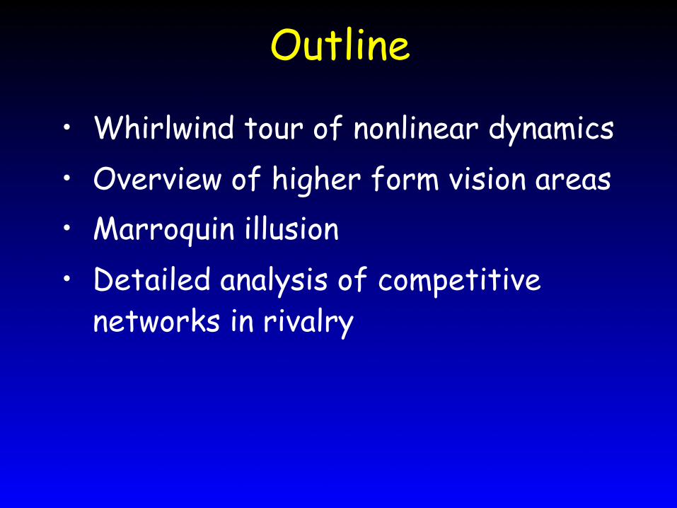
Linearized Stability Analysis

€

dxdt

= F(x,y)

dydt

=G(x,y)

€

J =

∂F∂x

∂F∂y

∂G∂x

∂G∂y

x,y=Equilibrium

• All real(eig) < 0, asymptotic stability• Any real(eig) > 0, unstable• Pure imaginary eig: theorem does not

apply

Nonlinear Oscillations• Limit cycles: cannot exist in linear systems• Only one general theorem: Hopf Bifurcation

Theorem• Conservative oscillations (analogous to

linear systems) can exist, but not in neural systems

• Chaos can occur in > 2 dimensions• All neural oscillations are limit cycles!

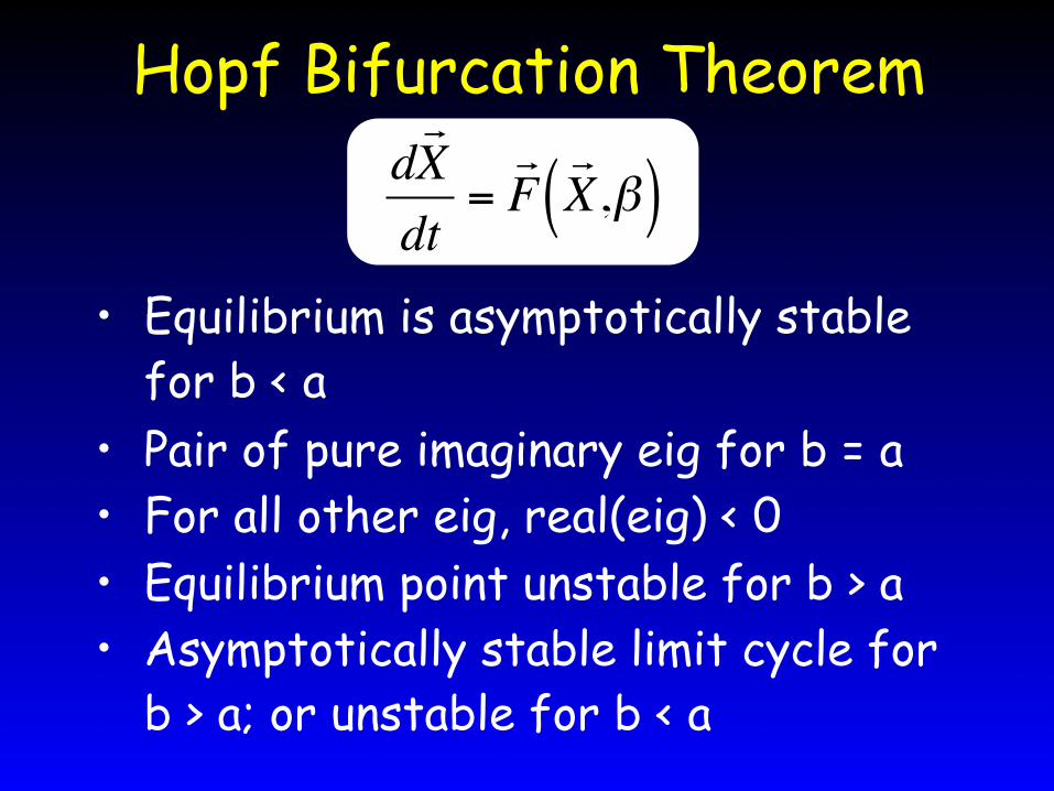
Hopf Bifurcation Theorem

• Equilibrium is asymptotically stable for b < a

• Pair of pure imaginary eig for b = a• For all other eig, real(eig) < 0• Equilibrium point unstable for b > a• Asymptotically stable limit cycle for

b > a; or unstable for b < a

€

dr X

dt=

r F

r X ,β( )

Hopf Addendum

• Limit cycle emerges with infinitesimal amplitude

• Frequency = Im(eig)/2pi• Hodgkin Huxley Euations exhibit

Hopf bifurcation

€

dr X

dt=

r F

r X ,β( )

Nonlinear Oscillations Caveats• Not all limit cycles emerge via Hopf

bifurcations• Example: Mammalian cortical neurons• Conservative oscillations (analogous to

linear systems) can exist, but not in neural systems

• Chaos can occur in > 2 dimensions• All neural oscillations are limit cycles!

Conduction & Spiking Dynamics

• Two-compartment model (Rinzel et al)• Excitatory neurons: slow AHP currents• Simple but accurate cubic model (Wilson, 1999)

dVdt = – a V2 – b V V – ENa – R V – EK + Iinput

τ Rd Rdt = – R + cV2

(conductance)x(potential)

Phase Plane & Spike Generation

-0.2 0 0.2 0.4 0.6 0.8-0.2

0

0.2

0.4

0.6

0.8

1

V

R

-0.2 0 0.2 0.4 0.6 0.8-0.2

0

0.2

0.4

0.6

0.8

1

V

R

0 10 20 30 40 50 60 70 80 90 100-0.1

0

0.1

0.2

0.3

0.4

0.5

0.6

0.7

0.8

0.9

V (N

orm

alize

d Un

its)

Time (arbitrary units)

Fit to Human Action Potentials

-80

-60

-40

-20

0

20

40

0 1 2 3

HumanEqn (9.10)

Pote

ntia

l (m

V)

Time (msec)

A

-80

-60

-40

-20

0

20

40

0 1 2 3

HumanEqn (9.10)

Pote

ntia

l (m

V)

Time (msec)

A

Foehring et al, 1991

Spike Rate Adaptation• Human excitatory cortical neurons:

slow hyperpolarizing current• Causes spike rate adaptation

dVdt = – a V2 – b V V – E Na – R V – EK – H V – EK +I

τ Rd Rdt = – R + cV2

τ Hd Hdt = – H + gV2 Very slow K+ current

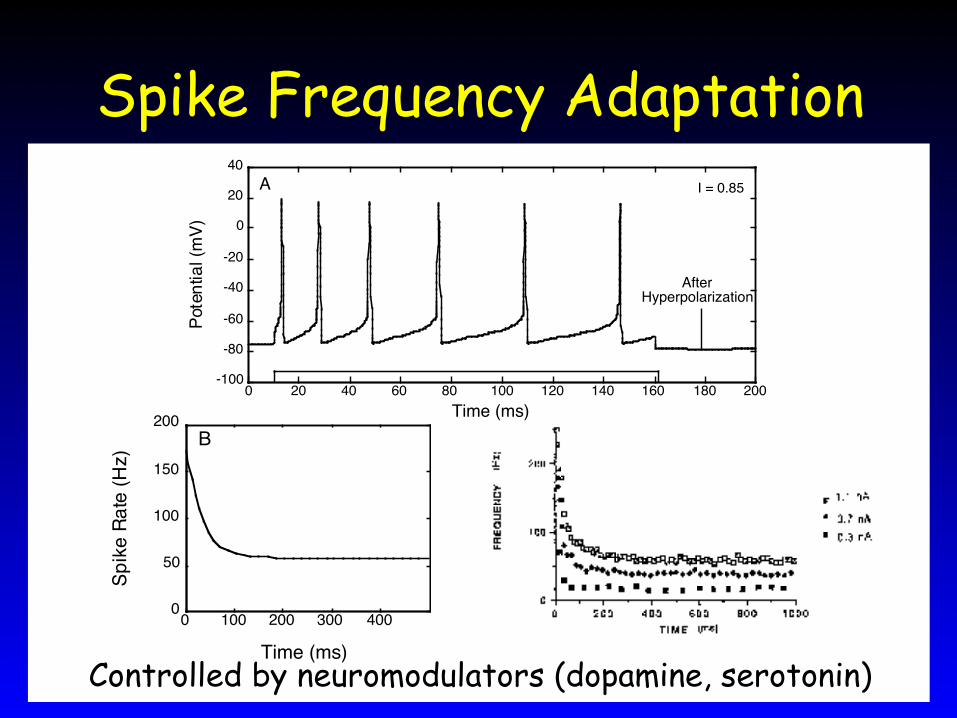
Spike Frequency Adaptation

0 100 200 300 4000

50

100

150

200

Time (ms)

B

Spik

e Ra

te (H

z)

0 20 40 60 80 100 120 140 160 180 200-100

-80

-60

-40

-20

0

20

40I = 0.85

Time (ms)

Pote

ntia

l (m

V)

AfterHyperpolarization

A

Controlled by neuromodulators (dopamine, serotonin)

Lyapunov Functions & Memory

• Positive definite function U(t) around an equilibrium

• dU/dt < 0 along trajectories in a region surrounding equilibrium

• Then equilibrium is asymptotically stable• Lyapunov fcns. always exist, but not unique

€

dUdt

=∂U∂xii

∑ dxidt

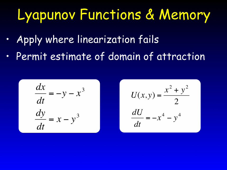
Lyapunov Functions & Memory• Apply where linearization fails• Permit estimate of domain of attraction

€

dxdt

= −y − x 3

dydt

= x − y 3

€

U(x,y) =x 2 + y 2

2dUdt

= −x 4 − y 4

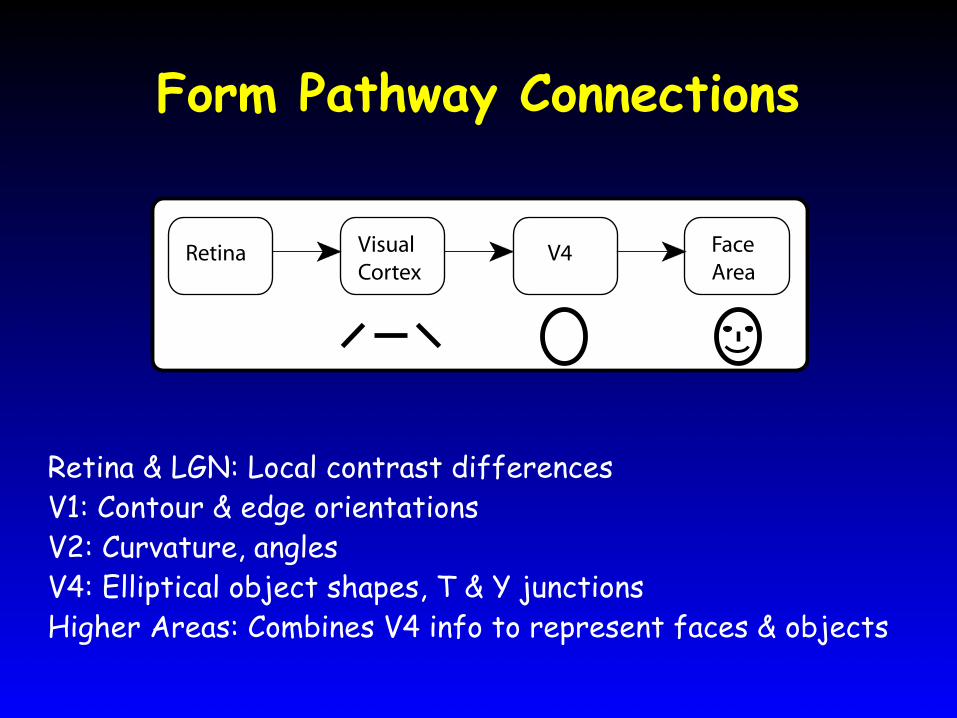
Form Pathway Connections

Retina & LGN: Local contrast differencesV1: Contour & edge orientationsV2: Curvature, anglesV4: Elliptical object shapes, T & Y junctionsHigher Areas: Combines V4 info to represent faces & objects

Retina VisualCortex

FaceArea

V4

Form Pathway Connections

Area to area feedback connectionsSkipping connectionsFeedback local but patchy

V1 V4 TEO TEV2

fMRI of V4

Wilkinson et al, Current Biology (2000)

V4 & FFA Activation

0

0.2

0.4

0.6

0.8

1

1.2

1.4

V1 V4 FFA

ConcentricRadialParallelFaces

Resp

onse

(% s

igna

l cha

nge)

Cortical Area

0

0.2

0.4

0.6

0.8

1

1.2

1.4

V1 V4 FFA

ConcentricRadialParallelFaces

Resp

onse

(% s

igna

l cha

nge)

Cortical Area

0

0.2

0.4

0.6

0.8

1

1.2

1.4

V1 V4 FFA

ConcentricRadialParallelFaces

Resp

onse

(% s

igna

l cha

nge)

Cortical Area

0

0.2

0.4

0.6

0.8

1

1.2

1.4

V1 V4 FFA

ConcentricRadialParallelFaces

Resp

onse

(% s

igna

l cha

nge)

Cortical Area

* *

**

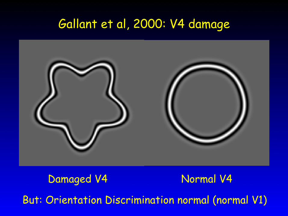
Gallant et al, 2000: V4 damage

Normal V4Damaged V4

But: Orientation Discrimination normal (normal V1)

Receptive Field Size Increases

0.1°

1°

10°

100°Receptive Field Sizes

RF DiameterKobatake & TanakaOp de Beeck et al

RF D

iam

eter

Cortical Area

Diameter = 0.09°·Area3.04

V1 V2 V4 TEO TE

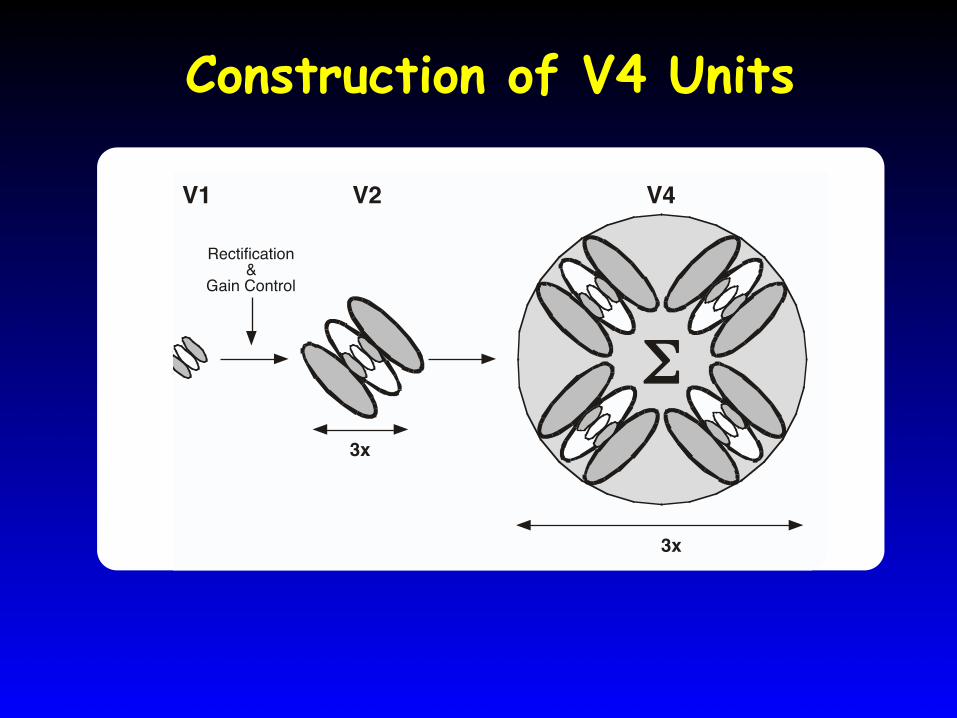
Construction of V4 Units

3x

3x

Σ

Rectification&

Gain Control

V1 V2 V4

3x

3x

Σ

Rectification&

Gain Control

fMRI & Distance from MeanMean Face

1

1.2

1.4

1.6

2 4 6 8 10 12 14 16Face geometry (%)

FFA neurons increase firing with distance from mean faceNature Neuroscience, October, 2005

Marroquin Illusion (1976)

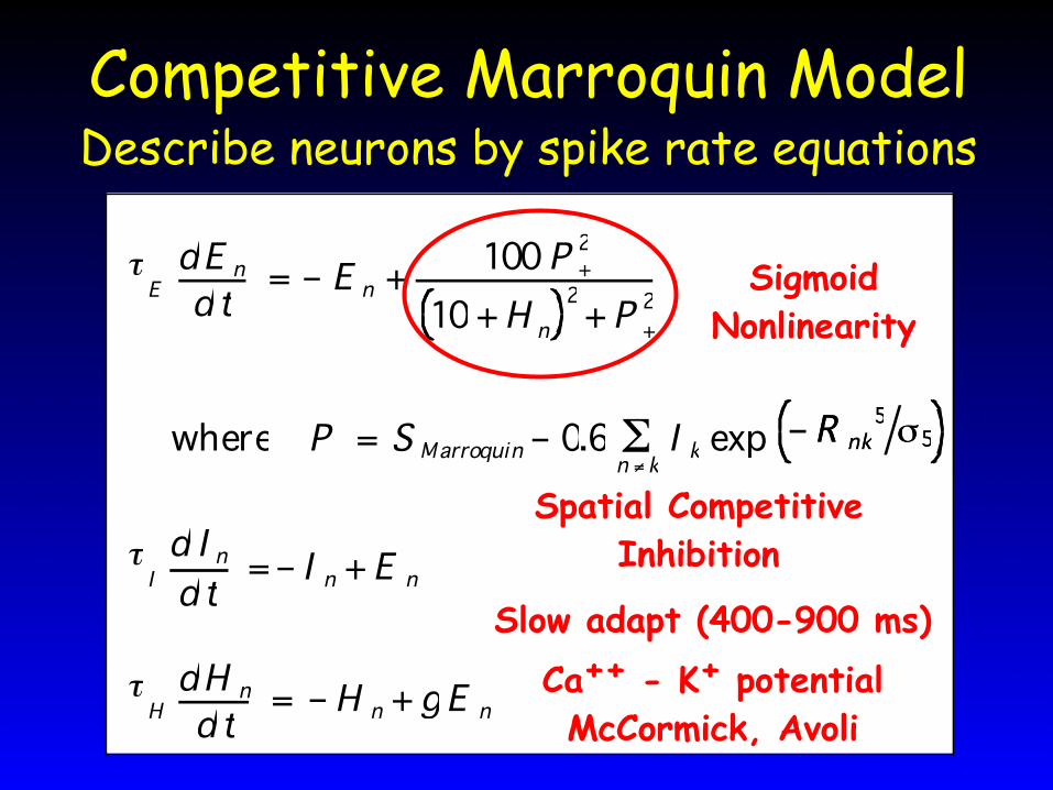
Competitive Marroquin Model

τEdE n

d t= – E n +

100P +2

10+H n2+P +

2

where P = S Marroquin – 0.6 I k exp – R nk5 σ5– R nk5 σ5Σ

n ≠ k

τId I n

d t= – I n + E n

τHdH n

d t= – H n +gE n

Slow adapt (400-900 ms) Ca++ - K+ potential McCormick, Avoli

Spatial Competitive Inhibition

Describe neurons by spike rate equations

Sigmoid Nonlinearity

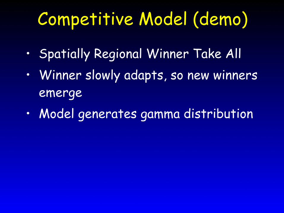
Competitive Model (demo)

• Spatially Regional Winner Take All• Winner slowly adapts, so new winners

emerge• Model generates gamma distribution

Gamma Distribution

0

5

10

15

20

0 2 4 6 8 10

FWGamma

Inte

rval

Cou

nt

Interval Duration (sec)

N = 103

0

10

20

30

40

50

60

70

0 2 4 6 8 10

ModelGamma

Interval Duration (sec)

N = 478

Too many long intervals for true Gamma!