J Fluid Mech (1994) uol 258 pp 191-216 Copyright 0 1994 Cambridge University Press

191

Nonlinear dynamics of viscous droplets By E BECKERT W J HILLER A N D T A KOWALEWSKIf

Max-Planck-Institut fiir Stromungsforschung Bunsenstrasse 10 D-37073 Gottingen Germany

(Received 9 July 1992 and in revised form 21 May 1993)

Nonlinear viscous droplet oscillations are analysed by solving the Navier-Stokes equation for an incompressible Auid The method is based on mode expansions with modified solutions of the corresponding linear problem A system of ordinary differential equations including all nonlinear and viscous terms is obtained by an extended application of the variational principle of Gauss to the underlying hydrodynamic equations Results presented are in a very good agreement with experimental data up to oscillation amplitudes of 80 of the unperturbed droplet radius Large-amplitude oscillations are also in a good agreement with the predictions of Lundgren amp Mansour (boundary integral method) and Basaran (Galerkin-finite element method) The results show that viscosity has a large effect on mode coupling phenomena and that in contradiction to the linear approach the resonant mode interactions remain for asymptotically diminishing amplitudes of the fundamental mode

1 Introduction The study of droplet dynamics can be traced back to the early work of Lord

Rayleigh (1879) Lamb (1932 pp 473-475 639-641) extended the inviscid linear analysis including weak dissipative effects and later Chandrasekhar (1961 pp 466477) solved the full viscous problem by mode analysis Subsequently Prosperetti (1977 1980u b) noted that the linear theory left open some questions about the initial value problem For example the amplitudes of Chandrasekharrsquos eigenfunctions are unknown for the oscillations of a deformed droplet starting from rest The analysis of initial vorticity generation first performed by Prosperetti is repeated here (in Appendix A) using a new formulation for the velocity field leading to an analytic solution for the problem

Although during the last decades nonlinear droplet dynamics has become the object of several theoretical and experimental investigations it remains one of the classical problems in hydrodynamics for which a complete theoretical solution is lacking However theoretical models describing particular aspects of nonlinear droplet dynamics have become very important in several applications for example in measuring fluid properties like surface tension and viscosity (Hiller amp Kowalewski 1989 Becker Hiller amp Kowalewski 1991) or in nuclear physics (Brosa amp Becker 1988 Brosa et uZ 1989) In particular the possibility of non-intrusive measurements of dynamic surface tension by the oscillating droplet method is of great interest for the determination of physico-chemical properties of liquid mixtures (Defay amp Petre 197 1

t Present address Institut fur Atmospharenphysik an der Universitat Rostock eV SchloBstr 4-6 D-18221 Kiihlungsborn Germany

$ On leave of absence from the Institute of Fundamental Technological Research Polish Academy of Sciences PL-00-049 Warszawa Poland

httpswwwcambridgeorgcoreterms httpsdoiorg101017S0022112094003290Downloaded from httpswwwcambridgeorgcore org 1 on 17 Mar 2017 at 053619 subject to the Cambridge Core terms of use available at

I92 E Becker W J Hiller and T A Kowalewski

Stiickrad Hiller amp Kowalewski 1993) Our experimental investigations of droplet oscillations have shown that linear theory as well as nonlinear inviscid theory have a very limited range of applicability in the interpretation of experimental results Hence our present interest is concentrated on the development of a nonlinear model including viscous effect which allows an easy analysis of experimental data enabling a calculation of the dynamic surface tension of the investigated liquids

The existing theoretical models describing nonlinear droplet dynamics either neglect viscosity (Tsamopoulos amp Brown 1983 Natarajan amp Brown 1987) or whilst taking viscosity into account use a strictly numerical approach (Lundgren amp Mansour 1988 Basaran 1992) The limitations of existing techniques have been widely discussed by Patzek et al (1991) It seems that two methods namely the boundary integral method applied by Lundgren amp Mansour (1988) and Galerkin-finite element method by Basaran (1 992) offer a reasonable approach to nonlinear and viscous droplet dynamics However these methods aside from their numerical complexity have limited practical applicability The boundary integral methods as was shown by Patzek et al (1991) cannot model droplet oscillations when the effects of viscosity are in the range that is physically of interest The finite element methods are limited at low viscosities (higher Reynolds numbers require fine discretizations and long computational time)

The new approach presented here offers the possibility of analysing nonlinear droplet dynamics for a wide range of nondimensional viscosity Furthermore it allows monitoring of the systematic errors of the algorithm by means of physically justified integrals

The present model of droplet oscillations (94) uses the mode expansion method with appropriate modes of the linear problem and takes into account all nonlinearities as well as viscosity This method is akin to the work of Boberg amp Brosa (1988) who analysed the transition to turbulence in a tube flow with the help of a corresponding mode expansion The existence of stationary boundary conditions in Boberg amp Brosarsquos problem allowed them to use Galerkinrsquos method to deduce their system of ordinary differential equations In the case of a free boundary problem the modes do not satisfy the boundary conditions a priori Therefore a direct application of semi-analytical methods becomes difficult Hence the problem of deriving an appropriate system of ordinary differential equations is solved by the use of the standard variational principle of Gauss This one of the most general principles of classical mechanics seems to be well suited to the analysis of nonlinear droplet oscillations since it offers the straightforward possibility of treating the boundary conditions as additional constraints on the Navier-Stokes (or the vorticity) equations For special cases if high- wavenumber modes of the droplet oscillation are strongly excited the method proposed in the present paper may become less appropriate compared with the aforementioned pure numerical solvers of Lundgren amp Mansour or Basaran However this limitation of our approach has no effect on its application to physical experiments with a free oscillating droplet where amplitudes of the oscillation modes are strongly related to their linear damping constants On the other hand our method is close to the physics of nonlinear droplet oscillations describing its dynamics in terms of the natural degrees of freedom This has been established both by the comparison of the computed droplet oscillations with experimental data given in Becker et al (1991) and repeating some droplet trajectories generated by Lundgren amp Mansour (1988) and Basaran (1992)

httpswwwcambridgeorgcoreterms httpsdoiorg101017S0022112094003290Downloaded from httpswwwcambridgeorgcore org 1 on 17 Mar 2017 at 053619 subject to the Cambridge Core terms of use available at

Nonlinear dynamics of viscous droplets 193

Il

z

FIGURE 1 A droplet cross-section described by the surface parametrization (21) The unit vcctors of the coordinate system as well as normal and tangential unit vectors of the surface are displayed The origin of the coordinate system is denoted by 0 and the centre of mass of the droplet by s

2 Formulation of the problem We consider an incompressible droplet of equilibrium radius T density p uniform

surface tension CT and kinematic viscosity v which is freely oscillating in a medium of negligible density and viscosity

In the mathematical description limited to axisymmetric droplet dynamics spherical coordinates ( I 8) are used where r is the distance from the system origin and 8 is the meridian angle measured from the axis of symmetry z As in our previous analysis (Becker et al 1991) we assume that the radial distance R(8 t ) from the origin of the coordinate system to the droplet surface can be expanded in a series of Legendre polynomials P(cos 0)

0

R(8t) = rua0(a2 a) + c a(t) p(cos )I (21)

Figure 1 illustrates the geometry Assuming constant liquid density R(8 t ) always encloses the same volume

(22)

This condition leads to a cubic equation defining the dimensionless mean droplet radius a as a function of the surface parameters a2 aT0 It turns out that a is always less than or equal to one The droplet shape is uniquely described by the parameters a ale They can be interpreted as dimensionless amplitudes of standing waves with 1 periods on strings encircling the cross-section of the droplet These waves oscillate independently of each other only in the linear case

The unit vectors normal (n) and tangential ( t ) to the droplet surface are given by the following formulae

(23)

2=2

1

fnr = 2x I- XR (8 t ) d cos 6

Re - a Re a Re + Re n = t = [R+(C0R)2]t [R2 + (ao R)]

where e and eH are unit vectors in the radial and the polar directions respectively In our experimental analysis (Becker et nl 1991) the surface parametrization (21)

yields the amplitudes a2 a the equivolumetric radius r and the position of the httpswwwcambridgeorgcoreterms httpsdoiorg101017S0022112094003290Downloaded from httpswwwcambridgeorgcore org 1 on 17 Mar 2017 at 053619 subject to the Cambridge Core terms of use available at

194 E Becker W J Hiller and T A Kowaiewski

coordinate system These parameters are fitted to the observed droplet shape However the origin 0 of the coordinate system does not need to coincide with the centre of mass s which may move along the symmetry axis z The displacement s of the centre of mass depends on the surface deformation and in the chosen coordinate system it is given by

(24) 10

s(u2 a 10 ) = gro 11 cos 6 ((a a) + C a ~ ( C O S 6) 1=2

The parameterization (21) does not include the term with index I = 1 because in our experimental analysis this term does not represent an additional degree of freedom for the description of the surface The amplitude a which in the linear theory describes a pure translational motion cannot be separated out in the experimental analysis Obviously it is possible to let a be different from zero and to require the centre of mass to coincide with the origin of coordinates This gives a second relation in addition to (22) which allows the elimination of a as a function of u2 az0 Both descriptions become equivalent if sr (or a) is small In practice the value of IsrI remains below 001 in our experimental and computational analysis

In the non-inertial coordinate system the Navier-Stokes equation for incompressible fluids has the following form

a u + (0 0) v-ie = - V p p - vV x V x v (25)

where v denotes the velocity field e the unit vector in the z-direction and p the pressure The acceleration of the coordinate system with respect to the centre of mass is equal to - j In the case of constant density p the governing equation (25) is equivalent to the vorticity equation ( V E )

aw = v x (u x w ) - v v x v x w w = v x 0 (26) Surface motion and flow velocity are coupled by the kinematic boundary condition (KBC)

v-(Re-cRe)= RcR r = R (27) The driving force of droplet oscillations namely the surface tension acts per- pendicularly to the free surface Therefore on the surface of the tangential stress of the flow vanishes and the normal stress balances the driving force The tangential stress condition (TSC) and dynamic boundary condition (DBC) become

( T n ) t = 0 (Tn)n = 2aH

r = R

r = R

T is the Newtonian stress tensor and H the mean curvature of the droplet surface The left-hand side of (28) contains only friction terms which are known from u The pressure p contained in the left-hand side of the dynamic boundary condition (29) is given by line integration of the Navier-Stokes equation (25)

Computational results are non-dimensionalized using ro and T = (pr33rr)i as scale factors for length and time

3 Linear oscillations of a viscous droplet A simple analytical method of finding partial solutions of linearized Navier-Stokes

problems was given by Brosa (1986 1988) These partial solutions applied below to describe linear oscillations of a viscous droplet were found to be also useful for

httpswwwcambridgeorgcoreterms httpsdoiorg101017S0022112094003290Downloaded from httpswwwcambridgeorgcore org 1 on 17 Mar 2017 at 053619 subject to the Cambridge Core terms of use available at

Nonlinear dynamics of viscous droplets 195

investigations of the corresponding nonlinear problem (4 4) In Appendix A results obtained previously by Prosperetti (1977 1980a) are recapitulated to illustrate the advantages of Brosarsquos modes ansatz

The partial solutions of the linearized Navier-Stokes equation in the case of rotational symmetry and free boundary conditions are given in the following form (Appendix B)

- - e - ~ t [b n v x v x v j j [ ( h rdquop r ] PJCOS S) + cp V ( r r J L q c o s O)] (31) and p = pit e-At ce(rrJ ~ ( C O S 0) (32)

al(t) = a e-Af (33) Owing to linearity a will have the same time dependence as D and p l

Inserting (31)-(33) into the linearized forms of the boundary conditions (27k(29) and making use of the orthogonality of the Legendre polynomials one obtains a homogeneous system of equations for the amplitudes bp cp and a The condition of non-trivial solutions for this system yields after several algebraic transformations

det(x) = 41(1-1)(l+2)-2x2+2 -(xj(x)) x dx

(35) a4 = -L2(riv)2 (36)

LIZ= (cFpr)l(Z- 1)(1+2) (37)

a 4 1 d +[-4Z(Z+2)(Z2- 1)+4Px2-x4+a4-2(1+ 1)a4~rsquo]j(x) = 0 (34)

[ x = (+)t rn

The characteristic equation (34) is equivalent to that given by Chandrasekhar (1961 chapter X equation (280)) 52 is the eigenfrequency in the case of an ideal fluid The existence of periodic solutions depends on the value of a21 which plays the role of an 1-dependent Reynolds number In the asymptotic case of small viscosity (lz21 + co) and oscillatory motion (x is complex) an analytical solution of (34) namely Lambrsquos irrotational approximation

follows In general the complex roots of det (x) must be found numerically Figure 2 shows the results for 1 = 2 For large values of 1a21 two conjugate roots are obtained When la21 increases from lazt( to infinity they form two branches in the complex plane of x These branches represent weakly damped oscillations In the limit laal + co the damping vanishes ie the relation IRe (x)Im (x)l becomes unity With decreasing la21 damping increases until both branches combine at x = xCTit (Id1 = Izfritl) and an oscillatory motion is no longer possible Further decrease of Ia21 leads to two real roots describing aperiodic decay of droplet deformations In the first case x tends to zero with 1a21 whereas in the second x tends to x In addition to this pair of solutions which depends strongly upon la21 there exists an infinite spectrum of nearly constant real roots These represent internal vortices of the droplet flow and give rise to strongly dissipative modes In figure 2 black squares mark the first three solutions It is surprising that these roots and therefore the corresponding velocity fields vary only weakly as la21 changes from zero to infinity The zero-maps for the higher wavenumbers ( I gt 2) look similar to that in figure 2

In contrast to the inviscid analysis the characteristic equation (34) has non-trivial solutions for Z = 1 This infinite set of real roots - not mentioned by other authors -

httpswwwcambridgeorgcoreterms httpsdoiorg101017S0022112094003290Downloaded from httpswwwcambridgeorgcore org 1 on 17 Mar 2017 at 053619 subject to the Cambridge Core terms of use available at

196 E Becker W J Hiller and T A Kowalewski

140

105

h Y - 70 E H

35

0

FIGURE 2 Map of roots of the characteristic equation (34) for polar wavenumber 1 = 2 The arrows indicate the direction of increasing a2

I I I X m t XO X11 X21 X31 X u -I1 ~ ~ ~ 1 387 744 107 139 171 - - -

X3f

2 369 189 267 532 3 882 285 40 663 4 154 371 516 789 5 236 451 625 911 6 332 529 729 103 7 444 606 832 115 8 571 681 933 126

- X4 i X 5 i X6l xl

886 122 154 186 102 136 168 200 115 149 182 214 128 162 196 228 141 175 209 242 153 188 222 255 165 201 235 269

TABLE 1 Ia~J xCrit co and the roots of the first five strongly dissipative modes for given polar wavenumbers 1 = 1 8 Owing to the weak dependence on a2 (for I k 2) the roots of the strongly dissipative modes are only approximate values

is independent of 121 and gives rise to strongly dissipative modes describing internal velocity fields which leave the droplet surface at rest In fact there are no a- deformations

Summarizing we obtain the discrete spectrum of eigenvalues

h( i= 12 l = 12 gt (39) characterized by radial and polar wavenumbers i and 1 Each pair of complex solutions is defined as A and Al where the imaginary part of A is supposed to be positive The additional damping constants of the strongly dissipative modes are enumerated with radial wavenumbers i 3 3 In the case of )a2) lt I C L ~ ~ ~ ~ or I = 1 only real eigenvalues occur they are numbered with monotonically increasing numbers i 2 1 The roots x iJ of (34) are labelled in the same way (see figure 2) Table 1 displays the most important values for polar numbers 1 = 1 8

httpswwwcambridgeorgcoreterms httpsdoiorg101017S0022112094003290Downloaded from httpswwwcambridgeorgcore org 1 on 17 Mar 2017 at 053619 subject to the Cambridge Core terms of use available at

Nonlinear dynamics of viscous droplets 197

The amplitudes byl c and al of the mode system can be found from the homogeneous equation system formed by the linerized boundary conditions As one of the amplitudes is arbitrary we can choose bl in a way that normalizes the partial solutions of the vorticity

wiL(r 0) e+ = b V x V x V x

(310)

(311)

In (310) eq = e x e denotes the unit vector in the azimuthal direction Defining

bJr 0) = bl V x V x

P(cosO)sinO (312) 1 cl(r 0) = Vyi(r 0) = V

+l rl-l

= e1P(cos0)-eoTP(cos0)sin0 (313) r0 yo

whereji denotes the derivative ofamp we can expand any linear droplet oscillation of the Ith surface mode in the following way

Each mode

(314)

(315)

contributes to surface deformation (afl) vortex flow (bi) and potential flow (c~ cJ

4 Mode expansion and dynamics of nonlinear droplet oscillations In this section we introduce a new approach to the nonlinear free boundary problem

(21)-(29) which allows us to find a semi-analytical solution by mode expansion and application of the variational principle of Gauss to the hydrodynamic equations It is based on the following premises

(i) The boundary conditions are used either to eliminate dependent variables or become additional constraints on the vorticity equation

(ii) The partial solutions provided by mode analysis must certainly be modified (iii) The linear and low viscous limits must result

httpswwwcambridgeorgcoreterms httpsdoiorg101017S0022112094003290Downloaded from httpswwwcambridgeorgcore org 1 on 17 Mar 2017 at 053619 subject to the Cambridge Core terms of use available at

198 E Becker W J Hiller and T A Kotvalewski

FIGURE 3 (a) Real and (b) imaginary part of the velocity field b (definition (312)) inside an undeformed droplet The dimensionless viscosity of Y = 001 123rT (la2] = 1454 in the case of 1 = 2) corresponds to droplets observed in our experiments

FIGURE 4 AS figure 3 but within a weakly deformed droplet and the lengthscale of the flow vectors is halved

The surface parameterization is given by (21) The mode expansions of the velocity field and vorticity contain several modifications

10 i o 10

4 y gt 0f) = c c Bz(t) bamp- 8 a a) + c c(O CI(Y a (41) z=1 i=l 1=1

First the fixed coupling c = c Bi cyl of the potential and vortex modes is removed In the linear analysis this coupling arises because the tangential stress of each velocity mode b + cl c vanishes at the undeformed droplet surface Obviously this cannot hold in the case of nonlinear deformations

Furthermore biz and wil become dependent on the surface parameters This modification generates reasonable vortex modes for arbitrary droplet shapes The former modes (310) are not appropriate as the spherical Bessel functions j with complex argument grow exponentially Therefore the vorticity of the weakly damped modes is concentrated in a sheet below the droplet surface (see figure 3) and its thickness vanishes with the damping This is a mathematical equivalent of Lambs irrotational approximation where potential flow inside the droplet and finite vorticity at the surface are assumed For the same reason the boundary layers of the modes (315) change significantly even if the deformations of the droplet are small (see figure 4)

It is expected that the boundary layers should adjust their structures to the actual droplet shape Indeed this is accomplished by modifying the argument of the spherical

httpswwwcambridgeorgcoreterms httpsdoiorg101017S0022112094003290Downloaded from httpswwwcambridgeorgcore org 1 on 17 Mar 2017 at 053619 subject to the Cambridge Core terms of use available at

Nonlinear djmanzics of uiscous droplets 199

Bessel functions in (312) substituting for ro the time- and angle-dependent droplet radius

yielding

Y Y

Figure 5 shows that the new vortex modes (45) behave as expected ie their boundary layers agree with the droplet surface Unfortunately the simple modification (44) not only results in rather complicated formulae for the derivatives of biz but it also produces singularities at the origin 0 In particular singularities of wiz V x V x bi and V x V x wil ep occur for I = 1 I = 12 and I = 123 respectively This is a result of the angle-dependent scaling of the radius r which produces distortions everywhere especially close to the origin We could avoid singularities at the expense of more complicated modifications and thus even more complicated formulae for the derivatives Therefore we keep the scaling (44) trying rather to eliminate the influence of singularities on the overall solution This is possible because the effects of vorticity are only relevant close to the surface Hence without losing accuracy we may split the droplet interior into two domains a little sphere of radius E surrounding the origin where we set the rotational part of the flow equal to zero and the rest where (45) is valid The thickness of the vortex layer depends on the viscosity therefore B should remain small compared to ro in order to assure validity of the solution for highly viscous liquids The irrotational approximation of Lamb and the nonlinear droplet model of Lundgren amp Mansour (1988) are limiting cases of this boundary-layer approximation

The potential modes cz (defined in (313)) were used previously to describe the inviscid flow in the nonlinear case (Becker et al 1991) They are taken without any modification

With the mode expansion (21) and (41 j defined so far the mean square errors of the governing equations (26)-(29) are defined in the following way

+ e - ( J ~ V x V x w - v x ( ( u x w ) ) ] ~ (47)

(481

(49)

[ u s (Re - z0 Re) - R 3 R] d cos 0

xsc = - 1 [(Tn)tI2dcos0 P V -1

x iBC = 1 l 1 [-(Tn)n-~H]dcos0 -1 P P

(410)

The problem is solved by minimizing the least-square error xFe of the vorticity equation with the constraints given by minimizing (48)-(410)

httpswwwcambridgeorgcoreterms httpsdoiorg101017S0022112094003290Downloaded from httpswwwcambridgeorgcore org 1 on 17 Mar 2017 at 053619 subject to the Cambridge Core terms of use available at

200 E Becker W J Hiller and T A Kowalewski

FIGURE 5 (a) Real and (b) imaginary part of b (definition (45)) within a weakly deformed droplet obtained with the viscosity and lengthscale of figure 3

It turns out to be appropriate to choose the surface parameters a and the amplitude Biz of the vorticity as independent variables Hence the amplitudes c of the potential flow as well as the time derivative bz and amp must be found by variation

The potential flow is determined by the tangential stress condition

xgsc = dcosB[ 3 3 B2(nV)bi +n x V x b - t 1=1 i=l

(41 1) The amplitude c cannot be evaluated from (411) because the tangential stress of the homogeneous flow cl=l vanishes We proceed eliminating c and the surface velocities u from the kinematic boundary condition

1 10 +x c12(nV)c) t +min

=$ 2xgscac1 = 0 I = 2 I 1=2

1=2 z=1 i = 1

axiBCac1 = 0 axiBCaul = 0 i = 2 I (412) The results of (411) and (412) can formally be written as

I i c1 = 2 2 C(aaogtBi I = 1 I (413)

a = C Z Ki(a a) Eim (414)

m-1 i-1

10 $0

I = 2 I m=1 z=1

4 i (415) -S=-C-u = - xS(a aogtBi

So far all expansion parameters for velocities and the first differential equations namely (414) are known

The accelerations ie differential equations of the form B = must be derived from the dynamic boundary condition (29) and the vorticity equation (26) in one step These equations are fundamentally of differing importance to the problem Whereas the vorticity equation plays its role only for viscous flow the driving force for oscillations - the surface tension - dominates droplet dynamics in general independent

as

1=2 aa m = l i = l

httpswwwcambridgeorgcoreterms httpsdoiorg101017S0022112094003290Downloaded from httpswwwcambridgeorgcore org 1 on 17 Mar 2017 at 053619 subject to the Cambridge Core terms of use available at

Nonlinear dynamics of viscous droplets 20 1

of the presence of viscous effects Therefore it is most important to satisfy the dynamic boundary condition with the smallest possible error Hence we must determine the unknown time derivatives Bi by minimizing the mean error x tBc without any regard to the value of xtE The remaining flexibility of the modes must be used to satisfy the vorticity equation

Accordingly we rewrite the dynamic boundary condition (29) substituting the pressure by line integration of the Navier-Stokes equation (25)

H (416) 2F 1 (a u - + ( v - V) o + Y V x V x u)dr + t + v(2(n V) u) n = - P

2 is a time-dependent constant of integration and equal to -2rpr in the linear limit By inserting expansion (41) into (416) the mean-square error (410) is transformed to

= dcos OFnc (417)

In (417) the lower integration limit r = 0 has been replaced by t in order to separate the singularities of the rotational modes (45) l$BC is the local error of the dynamic boundary condition

If viscous effects were absent the flow would be described by the velocity potential C c ~ alone In accordance with the boundary-layer argument the bulk Row can be considered as nearly irrotational in the case of damped oscillations also Hence x iBr become small if we choose formally the time derivatives i as variational parameters From (417) we see that this variation is equivalent to the projection of FDBC onto the potentials 91 Thus we obtain the following set of l + 1 independent equations from the dynamic boundary condition

(418)

Of course these additional constraints are calculated after inserting (413) into FDBC

2g P

( Y V X V X U - U X W ) ~ ~ - Y ~ ( ~ V ) V - ~ - - H (419)

Now the outstanding differential equations result simply from the variation xbE + rnin with the constraints (418)

h = 0 l = 0 1

httpswwwcambridgeorgcoreterms httpsdoiorg101017S0022112094003290Downloaded from httpswwwcambridgeorgcore org 1 on 17 Mar 2017 at 053619 subject to the Cambridge Core terms of use available at

202 E Becker W J Hiller and T A Kowalewski

The vorticity equation and dynamic boundary equation are weighted automatically because the set of equations (420) determines not only BtI and C but also the Lagrange multipliers K In the linear limit they become equal to zero The constraint (418) appearing as the first ( I -t 1) equations of (420) ensure the correct solution for the low viscous limit

Owing to the complex roots x ~ of the characteristic equation (313) the parameters determined by the minimization procedure are generally complex numbers To find real modes and real amplitudes every expansion containing the weakly damped modes or their derivatives must be rearranged to separate their real and imaginary parts For simplicity our notation describes full complex functions

The prime errors (47k(410) are normalized by referring them to the mean-square values of the corresponding functions that are approximated by the mode expansions

jl r r d r dcos 0 C C B(C w )+ep (vV x V x w - V x ( v x w)) X L e 1 = X L r1 Y1 7

(421)

1=17=1

These relations are used to measure the systematic errors of the governing equations

The final differential equations (414) and (420) are solved numerically applying the

(i) extrapolation in rational functions and polynomial extrapolation to evaluate

(ii) Gauss elimination to solve systems of algebraic equations (iii) a modified Runge-Kutta algorithin (Fehlberg 1970) to integrate ordinary

differential equations and (iv) approximation of the spherical Bessel functions by Legendre polynomials to

reduce computational time (Amos 1986) Finally let us consider the linear limit of the model We have chosen the surface

coefficients a and the vorticity amplitudes B a degrees of freedom Therefore one might expect inconsistency with the linear theory in which only the Bi are independent parameters and the a are always given by

(26)-(29)

following standard methods

integrals and derivatives (Stoer 1972)

Bila-a = 0 1 = 2 1 i= l

(425)

(see (314)) This problem would be avoided if the fixed relations (425) and their time derivatives were considered as additional constraints However a greater flexibility of the mode expansions seems preferable to us The example shown in figure 6 confirms

httpswwwcambridgeorgcoreterms httpsdoiorg101017S0022112094003290Downloaded from httpswwwcambridgeorgcore org 1 on 17 Mar 2017 at 053619 subject to the Cambridge Core terms of use available at

Nonlinear dynamics ojrsquo viscous droplets 203

00141 I A rsquo=

3 0 0 0 7 m

5 -0007 rsquo $ -00006

-0 oo 1 2

I - r(

0 2 4 6 8 0 2 4 6 8 Time (To) Time (To)

FIGURE 6 Computation in the linear limit Truncation numbers and initial conditions are i = 5 I = 2 a(O) = 002 and BJO) = 0 Thc radius of the irrotational region E = 0 lr and the dimensionless viscosity v = 0001 23r i T The solid curves show the results of the nonlinear model The dashed curves follow from linear theory (see (314)) They start at t = 036T and t = 117T indicated by solid vertical lines Their initial conditions are the actual values BJt) of the nonlinear numerical solution

that the present model behaves correctly in the linear limit The computation (solid lines) begins at initial conditions not allowed by (425) Comparisons with the linear solutions (dashed lines) following from (314) show initially some deviations However as can be seen these deviations disappear with time ie the nonlinear model approaches the linear solutions

5 Results 51 Initial conditions

Our experimental method of generating and evaluating oscillating droplets has already been described in recently published papers (Hiller amp Kowalewski 1989 Becker et al 1991) Strongly deformed axisymmetric droplets of about 05 mm in diameter are produced by the controlled breakup of a liquid jet and the time evolution of a droplet cross-section is observed using a stroboscopic illumination technique Further analysis consists of fitting the function (21) with a truncation number 1 = 5 to the recorded droplet shapes This yields the surface parameters a2 a5 and the equivolumetric radius Y as functions of time Usually the droplet radius decreases weakly with time owing to evaporation In the present model we neglect this small effect and assume for Y its mean experimental value

In the following we compare two typical experimental results already given in Becker ct al (1991 figures 5 and 6) with the theoretical predictions Figure 7 shows an example with large initial amplitudes

httpswwwcambridgeorgcoreterms httpsdoiorg101017S0022112094003290Downloaded from httpswwwcambridgeorgcore org 1 on 17 Mar 2017 at 053619 subject to the Cambridge Core terms of use available at

204 E Becker W J Hiller and T A Kowalewski

Time (ms) Time (ms) FIGURE 7 Experimental result for an ethanol droplet oscillating in air The surface parameters (dotted lines) a a5 are shown as functions of time Each dot corresponds to each time the droplet cross-section was recorded and analysed The mean equivolumetric radius of this measurement was r = 207 km t t and t mark points in time where computations with the model were started

The flow field inside the droplet cannot be determined experimentally Observations of droplets yield solely the surface parameters a and eventually their time derivatives ci (which can be evaluated by interpolating a(tj) Therefore it is difficult to formulate exact adequate initial conditions for the model However the a and ci contain more information than one might expect With the help of two additional assumptions it is possible to compute reasonable initial amplitudes Bi from the available experimental data These assumptions justified by comparison of numerical and experimental data are (i) the strongly dissipative modes can be neglected and (ii) the amplitudes obey the relations (425) These postulates correspond to the irrotational case where the velocity field is determined by the surface motion only Accordingly the tangential stress conditions (411 j yields

4 2

C = C C C (a a) Bim I = 2 I (51) m=2 6=1

and the kinematic boundary condition (412) can be rewritten in the form

xgBC = [d cos 0 [ (cl c + 1=2 i=l m=2

The couplings (425) now become additional constraints on (52) because variation of xfisc with respect to c1 and Bil gives only I independent equations Analogously to (420) we obtain the following system of algebraic equations

1 2

Kl = U - C u B = 0 I = 2 I = =I

All our nonlinear computations presented in the following sections were started using (53) to calculate initial conditions for the new model from the initial values of the surface parameters a and their velocities ci

httpswwwcambridgeorgcoreterms httpsdoiorg101017S0022112094003290Downloaded from httpswwwcambridgeorgcore org 1 on 17 Mar 2017 at 053619 subject to the Cambridge Core terms of use available at

Nonlinear dynamics of viscous droplets 20 5

a5

0 2 4 6 8 10 0 2 4 6 8 10 Time (To) Time (To)

FIGURE 8 Computational results (solid lines) starting at t (cf figure 7) Tn addition the experimental data (dotted lines) and the predictions of linear theory (dashed lines) are included The initial conditions and model parameters are a = 0 a = 0086 a = 0065 a5 = -003 Li = 09T aa = -031T a = -031T d = 018T v = 001123rT i = 3 1 = 6 and t = 0 1 ~ ~

52 Comparison with experiments In figure 7 t tL and t mark three zero crossings of a(t) separated in each case by two oscillation periods The experimental data at these points are used as initial conditions to start the calculation for the next interval Hence simulation of the whole experimental run is done in three steps covering three regions of droplet oscillations strong nonlinear (max laz(t)l z 06) nonlinear (max la(t)l z 04) and quasi-linear (max la(t)l z 02)

Calculations were performed using the physical data of the liquid used in the experiment ie p = 803 kgm3 B = 229 x in2s respect- ively The free parameters of the nonlinear model are chosen to be i = 3 I = 6 and E = 0 I r Although the large-amplitude oscillations were sometimes analysed experimentally with 1 = 10 amplitudes found for I gt 5 are too small to be evaluated with reliable accuracy The initial values of a6 and u6 have been set to zero as they are also not significant for the overall accuracy of the numerical analysis

Figure 8 shows results of the first computation starting at t They are compared with the experimental data and results of the linear model

Nm I = 149 x

al(0 = exp - Re ( A l l ) Q(A1 cos Im (All) tgt + A sin Im (A) t) (54)

where the constants A and A correspond to the initial values of a and CE The strongest nonlinearities are visible shortly after the droplet is generated at the

tip of the jet The maximum droplet deformation ie the maximum value of Ic all is approximately 08 One can see that unlike the case of the linear theory the present model describes the experimental data very well The following effects of nonlinearities can be readily seen when comparing with the linear model

(a) The oscillation period of the fundamental surface mode a increases The surface displacements are asymmetrical the maxima (prolate deformation) are larger and flatter whereas minima are sharper and have a smaller value These effects are also typical for inviscid nonlinear models (Tsamopoulos amp Brown 1983)

(b) The observed nonlinearity of the first higher-order mode a3 is even stronger it oscillates faster for negative displacements of a and clearly slower for positive ones The combined action of a and a3 shows that the average deformation of the droplet changes faster when the droplet has an oblate shape and slower when it is elongated These periodic frequency modulations can be understood in terms of effective masses In inviscid theory the kinetic energy of the droplet can be written as +ZMITnulhm

8 F L M 158 httpswwwcambridgeorgcoreterms httpsdoiorg101017S0022112094003290Downloaded from httpswwwcambridgeorgcore org 1 on 17 Mar 2017 at 053619 subject to the Cambridge Core terms of use available at

206 E Becker W J Hiller and T A Kowulewski

-002 0 2 4 6 8 10 0 2 4 6 8 10

Time (To) Time (To)

FIGURE 9 Computational results (solid lines) starting at t (cf figure 7) In addition the experimental data (dotted lines) and the predictions of linear thcory (dashed lines) are included The initial conditions are a2 = 0 a = 0026 a = 0009 a6 = 0001 a = 065T a = OO69T jl = -OO58T a = OOZZT The model parameters u i I F are those of figure 8

U4 003

-04 4 0 3

0 2 4 6 8 10 0 2 4 6 8 10 Time (To) Time (To)

FIGURE 10 Computational results of the nonlinear viscous model (solid lines) taken from figure 9 compared with a corresponding inviscid calculation (dashed lines) The solution of the inviscid model (Becker et al 199 1) has been evaluated with the maximum polar wavenumber l = 6 in the surface parametrization and velocity potential expansion

Each diagonal element of the mass tensor M gives the inertia of a single surface wave and the non-diagonal elements describe the nonlinear couplings Linearization leads to a diagonal matrix and effective masses M cc Sl(21+ 1) In the nonlinear case the matrix elements depend on the instantaneous droplet shape and it can be shown that a shape elongation yields growth of its diagonal elements

(c) The third higher oscillation mode u4 shows a strong coupling with u2 Except for the small ripple at t 2 3T the maxima of u4 coincide quite well with the extremes of u2 According to the linear analysis (compare (37)) one might rather expect the frequency ratio 1 3 instead of the observed ratio 1 2 and an arbitrary phase shift between both amplitudes This indicates that predictions of the linear theory cannot be related to the real behaviour of u4 This holds also for amplitude us although the mode coupling is not so straightforward

The predictions of the nonlinear model for the second interval t - t are shown in figure 9 Comparing it with the previous interval (figure S) one can see that the quantitative coincidence with the expcrimental data is clearly improved although the nonlinear characteristics remain The short-time behaviour of the oscillation amplitudes can also be relatively well described by the former inviscid nonlinear model (figure lo)

The results of the third computational run which starts at t are displayed in figure 11 together with both previous computations They are compared with the measured

httpswwwcambridgeorgcoreterms httpsdoiorg101017S0022112094003290Downloaded from httpswwwcambridgeorgcore org 1 on 17 Mar 2017 at 053619 subject to the Cambridge Core terms of use available at

Nonlinear dynamics of viscous droplets 207

a5

0 5 10 15 20 25 0 5 10 15 20 25 Time (To) Time (To)

FIGURE 11 Three successive computations (solid lines) starting at t t and t (cf figure 7) compared with the experiment (dotted lines) The discontinuity of the theoretical curves at t = 1 and t -= t is due to the restarting of calculations The initial conditions for t are up = 0 us = 00003 a4 = 00051 a5 = 0001 d = 0384T u = 0029T b4 = -00034T cis = -OO031T The model parameters v i I E are those of figure 8

$ T I J =I ri

5 10 15 20 25 0 5 10 15 20 25 0 N o

Time (To) Time (To)

FIGURE 12 Relative mean errors of the tangential stress conditions ( x ~ ~ + ) kinematic boundary condition (xamp+J dynamic boundary condition ( x amp ~ ~ ~ ) and vorticity equation (xF-gt (see definitions (421)-(424)) corresponding to the oscillation shown in figure 1 1

oscillation amplitudes It can be seen that the long-time behaviour of a and a3 shows oscillations typical of the damped harmonic oscillator Asymptotically both a and a3 approach the predictions of the linear theory Surprisingly even in this last-analysed interval the amplitude a remains always positive indicating the presence of the nonlinear mode coupling with a The surface wave a6 is not displayed as its small amplitudes are not of interest

Figure 12 shows the corresponding systematic errors (421)-(424) for the three calculation runs If strong nonlinearities are present the tangential stress condition and vorticity equation cannot be solved appropriately The maximum relative mean errors of these equations are of the order of 100 Nevertheless kinematic and dynamic boundary conditions which determine the droplet dynamics are always solved with negligible errors and the results are in accordance with the experiment This validates our approximation of treating the boundary conditions as additional constraints on the equation of motion The kinematic and especially the dynamic boundary conditions are essential for the irrotational inviscid droplet dynamics They remain dominant in the viscous case also The tangential stress condition and the vorticity equation seem to play a secondary role mainly affecting the amplitudes by damping

One example of modelling another experimental run characterized by moderate excitation amplitudes is shown in figure 13 (compare also figure 4 in Becker et al

8 - 2 httpswwwcambridgeorgcoreterms httpsdoiorg101017S0022112094003290Downloaded from httpswwwcambridgeorgcore org 1 on 17 Mar 2017 at 053619 subject to the Cambridge Core terms of use available at

208 E Becker W J Hiller and T A Kowalewski

f l 3

0 4 8 12 16 20 0 4 8 12 16 20 Time (To) Time (To)

FIGURE 13 Experimental (dotted lines) and theoretical (solid lines) results of an cthanol droplet oscillating at a moderate excitation amplitude The initial conditions are a2 = 0 a = 0061 a4 = 0042 a5 = -0002 a = 0625T a = -0065T a = 0085T as = -0103T The mean equivolumetric radius of the droplet = 01733 mm results in a dimensionless viscosity of Irsquo = 001227riT The other parameters are i = 3 I = 6 and e = 0 1 ~ ~ At t = t the observed droplet merges with a satellite

0101 I 0015 I

0 005 010 015 020

0005

a5 -0005

-0015

-0025 -0025 -0015 -0005 0005 0015

a2a3

FIGURE 14 Phase-space relations of mode couplings (a) between a4 and a (b) between aj and nB a3 The dots represent numerical results obtained with the present model taken from the data set of figure 11 for t gt ST The slopes of the fitted straight lines are (G) 047 and (b) 099

1991) At t = t x O S T the observed droplet merges with a satellite droplet It is interesting that this relatively violent disturbance has an appreciable influence only on the higher surface waves a and as However as time passes the severe deviations from the model predictions for these two amplitudes diminish Finally the experimental and theoretical data coincide again at least qualitatively This leads to the assumption that a4 and a are regenerated by nonlinear interactions with a2 and a3 and that their long- time behaviour is independent of initial disturbances

53 Mode couplings The mode interaction for a4 and a with initial conditions taken from the experiments can be simply analysed in the phase space These phase-space investigations have been done using a multi-parameter editor Relation (Wilkening 1992) In particular reasonable results seem to be offered by the relations a4 = a() and a = a5(a2a3) shown in figure 14 According to these representations the couplings of a4 and a can be approximately described by

a4 z C a and ub x C a as ( 5 5 ) httpswwwcambridgeorgcoreterms httpsdoiorg101017S0022112094003290Downloaded from httpswwwcambridgeorgcore org 1 on 17 Mar 2017 at 053619 subject to the Cambridge Core terms of use available at

Nonlinear dynamics of viscous droplets 209

010

005

0

4 0 5

4 10 0 2 4 6 8 1 0

010

005

0

-005

--010 0 2 4 6 8 1 0

Time

03

02

-01 0 ~ ~

-02

-03 0 2 4 6 8 1 0

010

i

005

0

i -005

-010 0 2 4 6 8 1 0

Time FIGURE 15 Calculated oscillations with weak viscous effects-compare with figures 7 and 8 of Lundgren amp Mansour (1989) The dimensionless viscosity of 7 = 40825 x 10-T corresponds to their Reynolds number of 2000 The time is scaled with (32)3 T The other model parameters are given in the text

Computations performed for several initial conditions (taken from experiments with ethanol and water droplets) indicate that these nonlinear couplings are in most cases the same and are approximately given by C z 045 and C z 09 The phenomena can be understood in terms of driving forces proportional to a and a a3 which are present in the differential equations for a4 and a5 The structures of these nonlinearity terms also follow from parity

Asymptotically the higher modes are always forced oscillators ie despite diminishing oscillation amplitudes the higher modes do not reach their linear solution (cf figure 11) This is because the damping increases with the wavenumber 1 (cf (38)) and within a short time the higher modes become dependent solely on the energy transferred from the fundamental mode Such a mode locking mechanism selected by the linear damping constants has already been described in Haken (1990 pp 21 1-217)

54 Additional computations and accuracy As was shown in the previous sections it is typical in experimental observations that the lower modes ( I = 23) contain most of the energy and that they are more or less the only degrees of freedom of surface motion The higher modes of lower energy are in

httpswwwcambridgeorgcoreterms httpsdoiorg101017S0022112094003290Downloaded from httpswwwcambridgeorgcore org 1 on 17 Mar 2017 at 053619 subject to the Cambridge Core terms of use available at

21 0 E Becker W J Hiller and T A Kowalewski

16

14

a - 12 b

10

08

06 0 4 8

Time 12

FIGURE 16 Transition from underdamped to critically damped conditions - compare with figure 12 of Basaran (1992) Variation of the dropletrsquos prolate aspect ratio ab = R(0 t)R(+n t) The time is scaled with t 3T Calculations for three dimensionless viscosities (Reynolds numbers) v = 57735 x 10-3rq (Re = 100) (solid line) v = 57735 x lO-rsquor7 (Re = 10) (dashed line) v = 57735 x lW1rT (Re = 1) (dotted line) The initial conditions are given in the text The other model parameters are i = 4 I = 6 and B = Olro

fact generated by strong nonlinear coupling with a2 and ug Such energy distributions clearly noticeable in the damping constants of Lambrsquos approximation (38) seem to be typical of natural droplet oscillations Of course one might propose any artificial initial condition

One interesting example with very low viscosity has been given by Lundgren amp Mansour (1989 figures 7 and 8) Their Reynolds number of 2000 corresponds to a dimensionless viscosity of v = 40825 x 10-4rT We have repeated their calculation with i = 3 lo = 8 and e = Olro using their initial conditions ie

a4(0) = 03 u4(0) = 0

and zero for the other surface modes The computed trajectories (figure 15) coincide quite well with those of Lundgren amp Mansour except for a slight discrepancy in the extreme values of the amplitudes The nonlinear characteristics are the same in both calculations second-order coupling of ua and u6 and third-order coupling of as with the energy carrier u4

Another comparison is shown in figure 16 We have repeated calculations of Basaran (1992 figure 12) for a droplet starting to oscillate with only the second mode excited ie a(O) = 04 u2(0) = 0 and zero for the other surface modes The computations have been performed for three difference viscosities (Basaranrsquos Reynolds numbers 100 10 and l) demonstrating transition from damped oscillations to an aperiodic decay

It is worth mentioning that all of Basaranrsquos nonlinear calculations showed aperiodic decay beyond a critical Reynolds number which closely corresponds to the critical

httpswwwcambridgeorgcoreterms httpsdoiorg101017S0022112094003290Downloaded from httpswwwcambridgeorgcore org 1 on 17 Mar 2017 at 053619 subject to the Cambridge Core terms of use available at

Nonlinear dynamics of viscous droplets 21 1 value given by the linear theory This justifies our approach of describing nonlinear droplet oscillations in terms of the linear modes

The accuracy of our numerical solutions depends on the truncation numbers io I and the assumed thickness of the vortex layer ( y o - amp ) It is rather difficult to find parameters justifying these values apriori To find the optimal truncation numbers and the optimal radius c several control calculations have been performed to analyse the influence of these parameters on the solution and its minimization errors (Becker 1991) It was found that for the cases analysed optimal values of in and 1 are 3 and 6 respectively Larger truncation numbers involve long computation times without significant improvement of the resulting accuracy The radius F of the zero-vorticity domain could be varied from 005 to 0 3 ~ ~ without noticeable deviations of the generated solutions

6 Concluding remarks A new droplet model for nonlinear viscous oscillations has been developed The

method is based on mode expansions with modified solutions of the linear problem and the application of the variational principle of Gauss Computational results are in accordance with experimental data and numerical calculations of other authors up to relative droplet deformations of 80 of the equilibrium radius Typical nonlinear characteristics like frequency modulation and mode coupling are found to be dominant even in the case of small deformations Consequently considerable discrepancies between the predictions of linear theory and the nonlinear dynamics are observed

The present droplet model cannot describe such strong effects as droplet rupture Also some fine details of the internal flow may become difficult to accurately model However our main interest namely experimentally observable droplet deformations are properly described over a wide range of the excitation amplitudes The method also allow a wide variation of the dimensionless viscosity (oscillation Reynolds number) describing both aperiodic decay of droplet deformations and oscillations with nearly vanishing damping This flexibility cannot be obtained easily by the available pure numerical methods

The evaluation of surface and volume integrals at every time step involves relatively long computation times limiting the applicability in solving practical problems However it has been found that with the help of the present model it is possible to construct simple differential equations which approximate the nonlinear behaviour of the surface parameters al(t) and reduce the computational time by two orders of magnitude Manipulating the coefficients of these equations ie surface tension and viscosity it is feasible to obtain within a short time an adequate description of the selected experimental data Such a model can be easily applied to measure dynamic surface tension and viscosity by the oscillating droplet method

This research was partially supported by the Deutsche Forschungsgemeinschaft (DFG) The authors wish to thank Priv-Doz Dr U Brosa Professor Dr F Obermeier and Dr A Dillmann for their suggestions and valuable discussions

Appendix A Looking at the linear solution given in 33 we can see the following problem How

can the amplitudes of the vorticity field Bi (315) be calculated if only the surface amplitude a and the velocity field vL are given a priori This question is not a trivial

httpswwwcambridgeorgcoreterms httpsdoiorg101017S0022112094003290Downloaded from httpswwwcambridgeorgcore org 1 on 17 Mar 2017 at 053619 subject to the Cambridge Core terms of use available at

212 E Becker W J Hiller and T A Kowalewski

one Consider a droplet at rest which starts to oscillate due to an initial surface deformation To solve this special problem we must know a non-trivial set of amplitudes Bi that combined with the velocities b + c c l assure a zero velocity field inside the droplet Obviously these amplitudes remain unknown without further analysis The reason is that any initial value problem is solved by mode analysis only if the system of equations is self-adjoint ie if all its eigenvalues are real

Let us apply Brosas (1986 1988) separation ansatz (euro3 3) in the following form

u(r 0 t) = v x v x (rB(r t ) q c o s H ) ) + C l ( t ) V((vr)l q c o s H ) ] (A 1)

The corresponding representation of the vorticity yields

1 V x q ( r 8 t ) = - - st B(r t ) Pi(cos 0) sin Be4 v

Thus an irrotational initial condition is given by

a(t = 0) bt(t = 0) B(r I = 0) = 0

Applying (A 1) to the linearized boundary conditions we obtain

(A 4) 21(P - I ) v I

4 r0

(a B(ro t ) - - B(r t)) + ii(t) + 28b(t) +Q2a(t) = 0

where the kinematic boundary condition has been used to eliminate c and i Because time and radius dependence have not been separated the function B(r t ) has to satisfy the diffusion equation

2 f(1+ 1) a B(r t ) + a B(r t)------ r2

which follow from the vorticity equation The dynamic boundary condition (A 4) ensures that for short times and irrotational

initial conditions every droplet oscillation obeys Lambs approximation (38) This holds independently of the value of v As the droplet starts to oscillate vorticity is generated at the surface owing to the tangential stress condition (A 5) For low fluid viscosity the vorticity cannot diffuse inside the droplet (the left side of (A 6) diminishes) and Lambs approximation holds during the full oscillation time This means that an irrotational initial condition is approximated by the weakly damped modes in the asymptotic limit of large Reynolds number 121 For larger viscosities the initial condition consists of both weakly damped and strongly dissipative modes The latter disappear quickly in time Hence as already shown by Prosperetti (1977) the long-time behaviour of the droplet will differ from the initial one

The analytical solution of the initial value problem (A 3)-(A 6) can be found using the standard Laplace transform method with the following conventions for a time function f and its Laplace transform 3

f (A) = r i i )e d t Re(A) lt 0 0

httpswwwcambridgeorgcoreterms httpsdoiorg101017S0022112094003290Downloaded from httpswwwcambridgeorgcore org 1 on 17 Mar 2017 at 053619 subject to the Cambridge Core terms of use available at

Nonlinear dynamics of viscous droplets 213 Re ($-is

27Ci Re (A)+ rz f ( t ) = 5 J f (h ) e-ht dh Re ( A ) lt 0

= - C Res f(h) ecntgt + - f(h) e-nt dh 2J3

The sum in the inversion formula (A 8 b) includes all residues of (A) e-ht with non- negative real parts of A The integral of (A 8 b) represents the counterclockwise integration along the infinite semicircle with positive real parts

Laplace transform of the system (A 4)-(A 6) with respect to the initial conditions (A 3 ) yields after several algebraic transformations

(A 9)

(A 10) 2(1- I ) r jL(xrr) Ci(O) + a(O) Q 2 A

i(rh) = lv det (x)

As expected the singularities of ii and Ecoincide with the solutions of the characteristic equation (34) A formula equivalent to (A 9) has already been given by Prosperetti (1977) who used a numerical method to obtain the inverse transform To invert (A 9) and (A 10) analytically we make use of (A 8b) and obtain

B(r t ) = a(O)

where ji and det denote the derivatives ofj(x) and det (x)

[bi + cz cI 1 I = i m are linearly dependent for I 2 2 The result (A 12) gives rise to the following interpretation the velocity modes

ie there is one non-trivial combination of the amplitudes namely

1 1 bio xiL det (xJ Bj K-

resulting in zero velocity Moreover A 12) yields

(A 13)

two non-trivial amplitude -

combinations for the vorticity modes (wit I i = 1 m which generate zero vortility for r lt r namely (A 13) and

However if we consider only a finite number of velocity or vorticity modes it turns out httpswwwcambridgeorgcoreterms httpsdoiorg101017S0022112094003290Downloaded from httpswwwcambridgeorgcore org 1 on 17 Mar 2017 at 053619 subject to the Cambridge Core terms of use available at

214 E Becker W J Hiller and T A Kowalewski

that they are linearly independent For polar wavenumber I = 1 the independence holds in general This flexibility of the mode system confirms the completeness of Brosas separation formulae

Appendix B In the case of constant fluid density and in the absence of bulk forces partial

solutions of the Stokes equation can be obtained as follows (Brosa 1986) The linearized Navier-Stokes equation

(B 1) 1

P at u(r t ) = --Vp(r t ) - vV x V x u(r t )

and the equation of continuity Vu(r t ) = 0

are solved using the following representations

u(r t ) = V x VP(r I ) ) + V x V x Vb(r t ) ) + V(c(r t ) )

p(r f) = -0 2t c(r 0 (B 3)

(B 4)

vV2P= ap vV2b = ab (B 5)

and the Laplace equation v2c = 0 (B 6)

V = + v r (B 7)

where the scalars p b and c must satisfy the diffusion equations

respectively The supporting vector field V is given by

where and I are arbitrary constants For the problem of droplet oscillations it is convenient to choose

V = r (B 8)

The partial solutions of (B 5 ) and (B 6) in spherical coordinates ( r 8 q5) are given by (Moon amp Spencer 1961)

P or b cc e - j [ ( ~ r l ~ ( 0 $1 c cc e-At(rro) qm(8 4)

(B 9) (B 10)

j denotes the spherical Bessel functions (Abramowitz amp Stegun chap 9) and qm the spherical harmonics In the case of rotational symmetry (rn = 0) the spherical harmonics can be substituted by the Legendre polynomials P(cos 0)

The velocity fields corresponding to (B 9) and (B 10) have the following forms

where e e and eo are the unit vectors in the radial polar and azimuthal directions httpswwwcambridgeorgcoreterms httpsdoiorg101017S0022112094003290Downloaded from httpswwwcambridgeorgcore org 1 on 17 Mar 2017 at 053619 subject to the Cambridge Core terms of use available at

Nonlinear dynamics of viscous droplets 215 The tangential stresses of the velocity modes (B 1 1)-(B I3) evaluated on a sphere

with radius yo are given by

for V x (rp)

for ~ x ~ x ( r b )

for V c

for V x (rp)

2 ($1 - a(a p - I r ) for V x (rp)

(za(a + br) + hv b) for v x v x (rb) (B 15)

for Vc

T denotes the Newtonian stress tensor of the corresponding velocity field According to (B 14) and (B 15) the tangential stresses of V x V x(rh) and V c depend on the angles of 6 and $ in the same way namely proportional to 2 qm in the ampdirection and proportional to (a$sin6) qm in the $-direction In the case of V x (rp) these dependencies are exchanged with respect to the (0 $)-components Hence this velocity mode produces tangential forces on the surface that cannot be balanced by the other modes The first term V x (rp) of the representation formula (B 3) therefore vanishes if free boundary conditions of a liquid sphere are considered

R E F E R E N C E S AEWMOWITZ M amp STEGUN I A 1968 Handbook ujMathematical Functions Dover AMOS D E 1986 A portable package for Bessel functions of a complex argument and nonnegative

BASARAN 0 A 1992 Nonlinear oscillations of viscous liquid drops J Fluid Mech 241 169-198 BECKER E 199 1 Nichtlineare Tropfenschwingungen unter Berucksichtigung von Oberflach-

enspannung und Viskositat (Nonlinear oscillations of viscous droplets driven by surface tension) Mitteilungen aus dem Max-Planck-Institut f u r Stromzingsforschung vol 104 E-A Miiller MPI Gottingen

BECKER E HILLER W J amp KOWALEWSKI T A 1991 Experimental and theoretical investigation of large-amplitude oscillations of liquid droplets J Fluid Mech 231 189-210

BOBERG L amp BROSA U 1988 Onset of turbulence in a pipe Z Naiurforsch 43a 697-727 BROSA U 1986 Linear analysis of the currents in a pipe 2 Naturfursch 41a 1141-1 153 BROSA U 1988 Strongly dissipative modes Unpublished paper Universitat Marburg BROSA U amp BECKER E 1988 Das zufallige HalsreiBen (Random Neck Rupture) Movie C 1694

available (in German or English) on loan from the IWF Nonnenstieg 72 D-37075 Gottingen Germany

BROSA U GROSSMANN S MULLER A amp BECKER E 1989 Nuclear scission Nuclear Phys A 502 4 2 3 ~ 4 4 2 ~

CHANDRASEKHAR S 1961 Hydrodynamic and Hydromagnetic Stability Clarendon DEFAY R amp euroTR~ G 1971 Dynamic surface tension In Sui$acr and Colloid Science (ed E

MatijeviC) pp 27-8 1 Wiley-lnterscience FEHLBERG E 1970 Klassiche Runge-Kutta-Formeln vierter und niedriger Ordnung mit

Schrittweitenkontrolle und ihre Anwendung auf Wiirmeleitungsprobleme Computing 6 61-71 HAKEN H 1990 Synergetik 3rd edn Springer

order ACM Trans Math Software 12 265-273

httpswwwcambridgeorgcoreterms httpsdoiorg101017S0022112094003290Downloaded from httpswwwcambridgeorgcore org 1 on 17 Mar 2017 at 053619 subject to the Cambridge Core terms of use available at

216 HILLER W J amp KOWALEWSKI T A 1989 Surface tension measurements by the oscillating droplet

LAMB H 1932 Hydrodynamics 6th edn Cambridge University Press LUNDGREN T S amp MANSOUR N N 1988 Oscillation of drops in zero gravity with weak viscous

MOON P amp SPENCER D E 1961 Field Theory Hundbook Springer NATARAJAN R amp BROWN R A 1987 Third-order resonance effect and the nonlinear stability of

PATZEK T W BRENNER R E BASARAN 0 A amp SCRIVEN L E 1991 Nonlinear oscillations of

PROSPERETTI A 1977 Viscous effects on perturbed spherical flows Q AppI Maths 35 339-352 PROSPERETTI A 1980a Normal-mode analysis for the oscillations of a viscous liquid drop immersed

PROSPERETTI A 1980h Free oscillations of drops and bubbles the initial-value problem J Fluid

RAYLEIGH LORD 1899 On the capillary phenomena of jets Proc R SOC Lond A 29 71-97 STOER J 1972 Einfuhrung in die Numerische Muthematik I Springer STUCKRAD B HILLER W J amp KOWALEWSKI T A 1993 Measurement of dynamic surface tension

by the oscillating droplet method Exp Fluids (to appear) TSAMOPOULOS J A amp BROWN R A 1983 Nonlinear oscillations of inviscid drops and bubbles

J Fluid Mech 127 519-537 WILKENING V 1992 Betrachtungen im Hyperraum - lsquoRelationrsquo verarbeitet Multi-parameter-

Daten crsquot 1 70-74

E Becker W J Hiller and T A Kowalewski

method Phys Chem Hvdrodyn 11 103-112

effects J Fluid Mech 194 479-510

drop oscillation J Fhid Meamp 183 95-121

inviscid free drops J Comput Phys 97 489-515

in another liquid J MPc 19 149-182

Mech loo 333-347

httpswwwcambridgeorgcoreterms httpsdoiorg101017S0022112094003290Downloaded from httpswwwcambridgeorgcore org 1 on 17 Mar 2017 at 053619 subject to the Cambridge Core terms of use available at
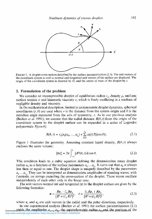
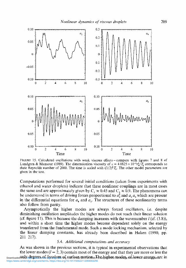
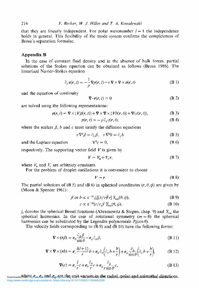